UNIVERSITY COLLEGE LONDON

University Of London Observatory DP20 – Diploma in Astronomy

Star Formation in Galaxies

Adapted from an original exercise by Dr. Phil James, Liverpool John Moores University. All data and images

come from this source.

Name:

An experienced student should aim to complete this practical in 1.5–2 sessions. It isexpected that you will have completed the “Classification of Galaxies and the HubbleDeep Field” exercise prior to attempting this.

1 Objectives

The aim of this exercise is to gain some practical understanding of star formation ingalaxies. You will look at many different types of galaxies and observe where starformation is occurring. You will then use a model–based relationship to estimate the totalstar formation rate and so draw up some general conclusions regarding star formationin galaxies.

2 Items required

Note that:

• You will need a web browser such as “Internet Explorer” or “Mozilla.”

• You will need to access the “Star Formation in Galaxies: Images” web page, whichis currently available on the Diploma in Astronomy website and CD-ROM underthe appropriate section of the laboratory scripts page.

• You may find it helpful to have a copy of the “Classification of Galaxies and theHubble Deep Field” script available.

A copy of Table 1 on page 11 is available as an Excel spreadsheet from any ULOWindows PC, by following the Star Formation - Diploma shortcut on the Windowsdesktop. A copy is also available on the Diploma website and CD-ROM.

You can save your work at any time in the directory diploma/student/year2/yourname

on the Win-apps network drive. (Ask a senior demonstrator to set up a directory foryou, if you cannot access it.)

1

3 Star Formation and the ISM

We often think of the space between stars as a vacuum, but in fact it is populated with avery tenuous mixture of dust and gas. This is known as the ‘interstellar medium’ (ISM).It is from this material that stars eventually form.

3.1 Interstellar Dust

Interstellar dust makes up about 1% of the ISM (in our galaxy) by mass and yet it isthought that there is only one dust particle per 10 6m3. Even at this low density, thedust grains have a noticeable effect on the light that we observe from space. This isbecause dust grains contribute greatly to the opacity1 of the ISM, causing noticeable‘reddening’ and dimming of the stars that we observe.

3.1.1 Interstellar Reddening

Astronomers sometimes describe the distance to an object in terms of its so–calleddistance modulus; m−M , where m is the apparent brightness of the object as measuredfrom the Earth and M is the brightness of the object as measured from a distance of 10parsecs. Both m and M are in magnitudes.

When light passes through the ISM, a proportion of it is absorbed and scattered byintervening dust grains. This makes objects appear fainter; i.e. m is numerically larger.Astronomers take account of this interstellar absorption by applying a correction tothe distance modulus known as the absorption coefficient, A. With this correction, thedistance modulus can be related to the actual distance, d, in parsecs using Equation 1below.

m−M = 5 log d− 5 + A (1)

A is observed to depend on wavelength. The dust grains scatter light differently atdifferent wavelengths; this is selective scattering. More light is scattered in the blue partof the spectrum than in the red so the light from a star will appear artificially reddenedwhen viewed from the distant Earth.

If the interstellar dust grains were distributed evenly all over space, we would simplybe able to assume that A = kd where k is a constant. The fact that observationally thisis not true leads us to the conclusion that the dust must be unevenly spread; i.e. it isclumpy.

3.1.2 Dark Nebulae

We can observe this ‘clumpiness’ directly in some nebulae, such as the famous ‘HorseheadNebula’ in Orion (shown in Figure 1).

The Horsehead Nebula is a ‘dark’ nebula. Dark nebulae are opaque clouds of dust(and gas) and often form near, to or are indeed superimposed on, to bright nebulae.Sometimes very small dark nebulae form, called globules. These are visible as darkspecks on bright nebulae.

1Opacity is a measure of the fraction of light absorbed by a material per unit distance.

2

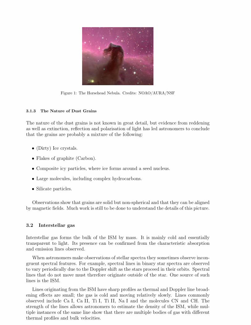
Figure 1: The Horsehead Nebula. Credits: NOAO/AURA/NSF

3.1.3 The Nature of Dust Grains

The nature of the dust grains is not known in great detail, but evidence from reddeningas well as extinction, reflection and polarisation of light has led astronomers to concludethat the grains are probably a mixture of the following:

• (Dirty) Ice crystals.

• Flakes of graphite (Carbon).

• Composite icy particles, where ice forms around a seed nucleus.

• Large molecules, including complex hydrocarbons.

• Silicate particles.

Observations show that grains are solid but non-spherical and that they can be alignedby magnetic fields. Much work is still to be done to understand the details of this picture.

3.2 Interstellar gas

Interstellar gas forms the bulk of the ISM by mass. It is mainly cold and essentiallytransparent to light. Its presence can be confirmed from the characteristic absorptionand emission lines observed.

When astronomers make observations of stellar spectra they sometimes observe incon-gruent spectral features. For example, spectral lines in binary star spectra are observedto vary periodically due to the Doppler shift as the stars proceed in their orbits. Spectrallines that do not move must therefore originate outside of the star. One source of suchlines is the ISM.

Lines originating from the ISM have sharp profiles as thermal and Doppler line broad-ening effects are small; the gas is cold and moving relatively slowly. Lines commonlyobserved include Ca I, Ca II, Ti I, Ti II, Na I and the molecules CN and CH. Thestrength of the lines allows astronomers to estimate the density of the ISM, while mul-tiple instances of the same line show that there are multiple bodies of gas with differentthermal profiles and bulk velocities.

3

3.3 Giant Molecular Clouds

Observations show that the bulk of the material in the ISM is bound up into GiantMolecular Clouds (GMCs). The typical properties of a GMC can be summarised thus:

• GMCs consist mainly of hydrogen, in molecular form (H2), but with a small masscontribution from a large variety of other molecular types.

• The clouds have relatively large densities with approximately 1000, 000, 000 moleculesper cubic metre.

• GMCs are often very large, of order 10 parsecs.

• The total mass of an individual cloud can be thousands or even millions of timesthe mass of the Sun.

The collapse of a GMC leads to a burst of star formation. Possible triggers for thecollapse include the shock waves caused by a supernova, or gravitational perturbations.The mass of material effected by these disturbances must exceed the Jeans Mass forcollapse to occur.

Once a cloud starts to collapse, it fragments into regions of high density. It is theseregions in which star formation occurs.

3.4 H II Regions

When neutral hydrogen (H0) is exposed to radiation with a wavelength shorter than91.2nm it ionises (i.e. loses its electron to become a positively charged nucleus) toform H+. If a cloud of gas has a hot star embedded in it, the surrounding gas willionise, forming a so–called HII region (pronounced ‘aitch–two’). When ionised hydrogengas recombines, by capturing an electron, a photon is released. The dominant opticalemission line in this process is called Hα (H-alpha) and it is this line that the exercisewill be looking at.

The presence of an H II region is a good indicator of star birth. This is becausehydrogen can only be ionised en masse by hot massive stars. These stars are short livedand do not have time to move far out of their natal clouds, as in Figure 2. So if we seestrong Hα emission in an object, we know that there is a good chance that there is starformation occurring nearby.

4

Figure 2: A star formation region in 30 Doradus shown at both infrared and optical wavelengths. Atinfrared wavelengths, radiation can penetrate the dust clouds, so that the formation regions are visible.Notice the tightly bunched pockets of stars. The arrows indicate stars not visible on the optical image.These are stars still shrouded in their natal clouds. Credits: NASA/ST–ScI

4 Measuring Star Formation Rates

As discussed in §3.4, Hα line emission is usually a good indicator of star formation. Wecan estimate the star formation rate (SFR) in an entire galaxy using Equation 2, whereLHα is the observed total emitted luminosity of the galaxy in Hα and is measured inWatts (W) and the SFR is measured in solar masses per year (M� yr−1).

SFR = 7.9× 10−35LHα (2)

Figure 3 shows NGC 1241 and NGC 1242 when taken through both a narrow–bandHα filter, 3(a), and a broad–band optical filter, 3(b).

(a) Hα (b) Optical

Figure 3: NGC 1241 (right) and NGC 1242 (left). Credits: Dr. Phil James, LJMU

5

Compare the images of NGC 1241 in Figures 3(a) and 3(b). This is a large spiralgalaxy with well defined arms. In Figure 3(b) only the central nucleus and parts of thespiral arms are visible. This is because only these parts of the galaxy are strong Hαemitters. We can conclude from this that most of the star formation is occurring inthese places. If we look at Figure 3(b), we can see the overall structure of the galaxy. Itseems that star formation is only happening in the very central ‘lane’ of the arms, andin the central core of the nucleus.

We can estimate the SFR for NGC 1241 by referring to Table 1 on page 11. Thetotal Hα flux, F, was measured to be 1057.5× 10−18Wm−2 while the measured recessionvelocity, v, was 4022kms−1.

4.1 Calculations

We want to calculate the total luminosity of the Hα lines. To do this we need to estimatethe distance to the galaxy. We can make a crude estimate of this using Hubble’s Law(Equation 3).

R =v

H0

(3)

Here, R is the distance to the galaxy in Mpc (1 pc = 3.26 ly = 3.086 × 1016m), v isthe galaxy’s recession velocity in km s−1 and H0 is Hubble’s constant. Recent resultsgained from the WMAP satellite and independently from the Hubble Space Telescopehave shown that:

H0 = 72+4−3km s−1Mpc−1

Applying Equation 3 in SI units we find for NGC 1241:

R =v

H0

× 3.086× 1022m Mpc−1 =4022km s−1

72km s−1Mpc−1× 3.086× 1022m Mpc−1

so that

R = 1.72× 1024m

LHα for this example is given by Equation 4:

LHα = 4πR2F = 4π ×(1.72× 1024m

)2× 1057.5× 10−18Wm−2 = 3.93× 1034W (4)

We need to correct this result for absorption of Hα photons by dust (multiply by 2.8– a rough but reasonable estimate of the effects of absorption), but we must first removethe flux from nearby nitrogen lines in the spectrum, which enhance the total emission.The nett correction is obtained by multiplying LHα by two.

LHα × 2 = 7.86× 1034W

Using this result we can calculate the SFR using Equation 2. In this case we obtain:

SFRNGC 1241 = 6.2M� yr−1

6

Exercise and Questions

Q.1 In §3.3 it is stated that for GMC collapse to occur, the mass of material affectedby a perturbation must exceed the Jeans mass, for which the equation is givenbelow:

Mj ≈kT

GmR

k is the Boltzmann constant, G is the gravitational constant, T is the temper-ature of the cloud and R is its radius. m is the average mass of a particle inthe cloud. This can be re-expressed in terms of a density, the Jeans density :

ρj ≈1

πM2

[kT

Gm

]3

This gives the minimum density for which gravitational collapse of a GMC canoccur.

k = 1.38× 10−23JK−1 G = 6.67× 10−11Nm2 kg−2 mH = 1.67× 10−27kg

a) Calculate ρj for a cloud with a mass of 2 × 1034kg and a temperature ofT = 30K. You may assume that m = 2mH

b) The average density of the ISM is approximately 1 × 10−27kg m−3. Howmany times greater is ρj than this?

c) What can we conclude from this about star formation in the ISM?

7

Q.2 Open the “Star Formation in Galaxies: Images” web page in your browser. 31fields are shown taken through both a narrow band Hα filter and a broad bandred filter. The image on the left of each page is the Hα image, while the oneon the right is the red image. The Hα image highlights star formation regionsin each galaxy.

a) Look at all the images provided and classify each galaxy according to thede Vaucouleurs scheme. You may need to refer to the “Classification ofGalaxies and the Hubble Deep Field” script to remind yourself of this.Make a note of your classifications in the table at the end of this script.

b) Make notes on where, in each galaxy, star formation is occurring. You canenter comments on this in the table at the end of the script.

c) How much star formation is happening in each galaxy? Assign each galaxyin the list a star formation rating, so that galaxies with no visible starformation are given 0 and galaxies with very active star formation aregiven 10. Enter this into your table.

d) Use the procedure given in §4 and the data in Table 1 to calculate anapproximate star formation rate (SFR) for each galaxy. Enter this intoyour table. You may want to produce a spreadsheet to help you with this.

8

Q.3 Look at the table that you have produced and answer the following questions:

a) Which types of galaxies generally show the most star formation? Considerboth the images and the star formation rates that you have calculated.

b) Comment on where star formation occurs in spiral galaxies. Can you thinkof any reasons why it might occur in these places?

c) Comment on star formation in elliptical galaxies. Compare the amount ofstar formation to that in spiral galaxies. Can you explain this difference?

d) Do you think that the method you have used to calculate the star forma-tion rate for each galaxy produces good results? Do your star formationratings correlate well with the SFR values you have calculated?

Hint: To answer this question you should plot a graph of your SFR valuesagainst your star formation ratings. The star formation ratings must beadjusted for distance by multiplying each star formation rating by R2

where R is the distance to that galaxy.

9

5 References

• James, P. Measuring star formation in interacting galaxies, LJMU.http://www.livjm.ac.uk/learning/postgrad/science/ast/astrocpd/9113.asp

Taken from the course CD-ROM.

• Kennicut, Jr., R. C., Annual Review of Astronomy and Astrophysics, v36, pp 189-231,1998.

• Spergel, D.N. et al, First Year Wilkinson Microwave Anisotropy Probe (WMAP)Observations: Determination of Cosmological Parameters, ApJ.http://arxiv.org/abs/astro-ph/0302209

• Zeilik, M. & Gregory, S. Introductory Astronomy and Astrophysics, (4th edition).The 3rd edition, by Zeilik, Gregory & Smith, is very similar. §P5–5 and §15

Authors: Will Reece, Mike Dworetsky, August 2003.

10

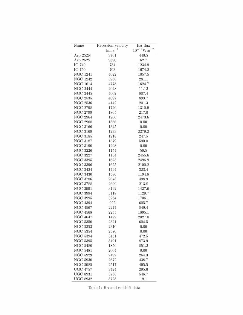
Name Recession velocity Hα fluxkm s−1 10−18Wm−2

Arp 252N 9761 440.5Arp 252S 9890 62.7IC 749 784 1234.9IC 750 703 1674.2NGC 1241 4022 1057.5NGC 1242 3938 281.1NGC 1614 4778 1624.7NGC 2444 4048 11.12NGC 2445 4002 807.4NGC 2535 4097 893.7NGC 2536 4142 201.3NGC 2798 1726 1310.9NGC 2799 1865 217.0NGC 2964 1266 2473.6NGC 2968 1566 0.00NGC 3166 1345 0.00NGC 3169 1233 2279.2NGC 3185 1218 247.5NGC 3187 1579 590.0NGC 3190 1293 0.00NGC 3226 1154 50.5NGC 3227 1154 2455.6NGC 3395 1625 2496.9NGC 3396 1625 2100.2NGC 3424 1494 323.4NGC 3430 1586 1194.8NGC 3786 2678 498.9NGC 3788 2699 213.8NGC 3991 3192 1427.6NGC 3994 3118 1129.7NGC 3995 3254 1706.1NGC 4394 922 605.7NGC 4567 2274 849.4NGC 4568 2255 1895.1NGC 4647 1422 2027.0NGC 5350 2321 604.5NGC 5353 2310 0.00NGC 5354 2570 0.00NGC 5394 3451 472.5NGC 5395 3491 873.9NGC 5480 1856 851.2NGC 5481 2064 0.00NGC 5929 2492 264.3NGC 5930 2672 438.7NGC 5985 2517 495.5UGC 4757 3424 295.6UGC 8931 3738 546.7UGC 8932 3728 19.1

Table 1: Hα and redshift data

11

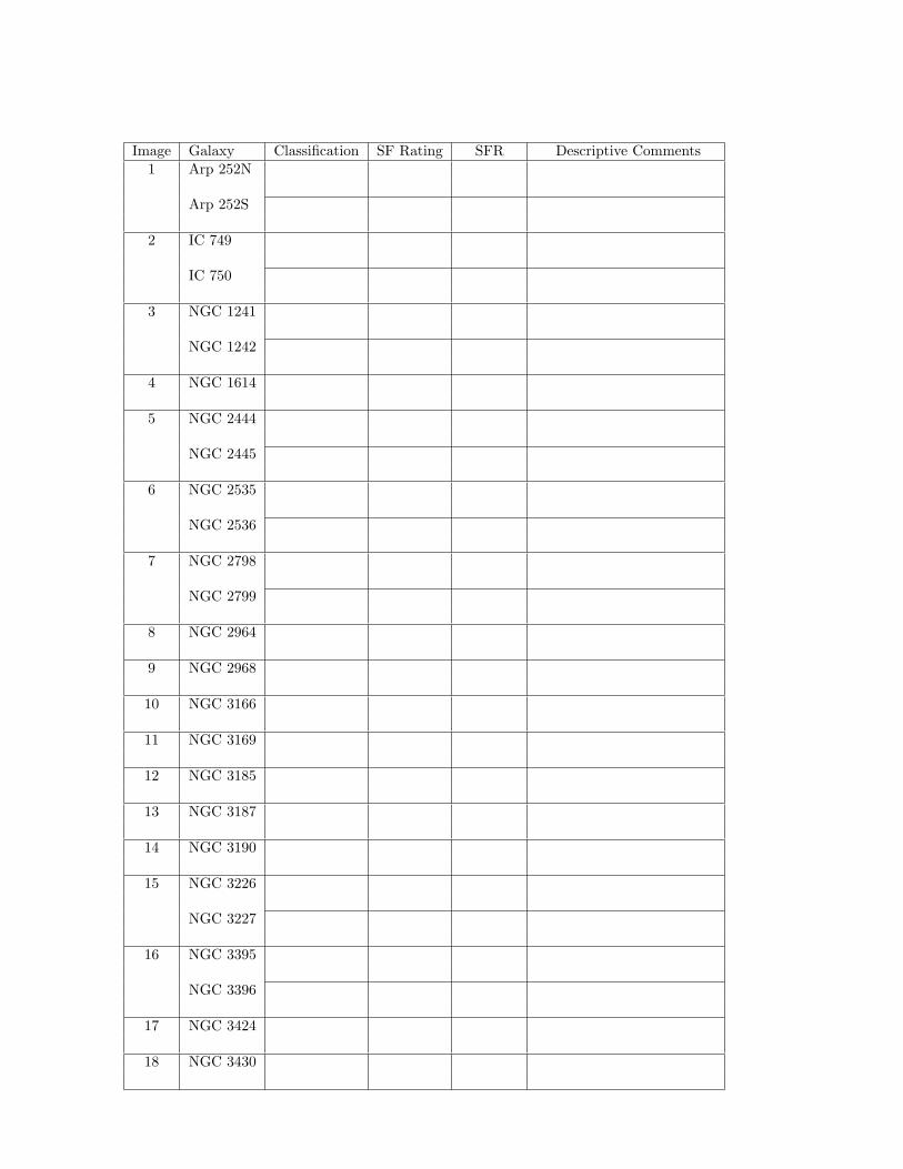
Image Galaxy Classification SF Rating SFR Descriptive Comments1 Arp 252N

Arp 252S

2 IC 749

IC 750

3 NGC 1241

NGC 1242

4 NGC 1614

5 NGC 2444

NGC 2445

6 NGC 2535

NGC 2536

7 NGC 2798

NGC 2799

8 NGC 2964

9 NGC 2968

10 NGC 3166

11 NGC 3169

12 NGC 3185

13 NGC 3187

14 NGC 3190

15 NGC 3226

NGC 3227

16 NGC 3395

NGC 3396

17 NGC 3424

18 NGC 3430

12

Image Galaxy Classification SF Rating SFR Descriptive Comments19 NGC 3786

NGC 3788

20 NGC 3991

NGC 3994

NGC 3995

21 NGC 4394

22 NGC 4567

NGC 4568

23 NGC 4647

24 NGC 5350

25 NGC 5353

NGC 5354

26 NGC 5394

NGC 5395

27 NGC 5480

NGC 5481

28 NGC 5929

NGC 5930

29 NGC 5985

30 UGC 4757

31 UGC 8931

UGC 8932

13