university college london - ucl discoverydiscovery.ucl.ac.uk/16280/1/16280.pdf · 1 fracture...
TRANSCRIPT
1
Fracture mechanics of volcanic eruptions
This thesis is submitted for the degree of Doctor of Philosophy at
University College London
Clare Matthews
January 2009
Department of Earth Sciences
University College London
Gower Street
London
WC1E 6BT

2
Declaration
I, Clare Matthews, confirm that the work presented in this thesis is my own. Where
information has been derived from other sources, I confirm that this has been indicated
in the thesis.
Signed ................................................................
Date ................................................................

3
Abstract
Seismology is a key tool in the forecasting of volcanic eruptions. The onset of an
eruption is often preceded and accompanied by an increase in local seismic activity,
driven by fracturing within the edifice. For closed systems, with a repose interval of the
order of a century or more, this fracturing must occur in order to create a pathway for
the magma to reach the surface. Time-to-failure forecasting models have been shown to
be consistent with seismic acceleration patterns prior to eruptions at volcanoes in
subduction zone settings. The aim of this research is to investigate the patterns in
seismic activity produced by a failure model based on fundamental fracture mechanics,
applied to a volcanic setting. In addition to the time series of earthquake activity,
statistical measures such as seismic b-value are also analysed and compared with
corresponding data from the field and laboratory studies. A greater understanding of the
physical factors controlling fracture development and volcano-tectonic activity is
required to enhance our forecasting capability.
The one dimensional, fracture mechanics grid model developed in this work is
consistent with the theory of growth and coalescence of multi-scale fractures as a
controlling factor on magma ascent. The multi-scale fracture model predicts an initial
exponential increase in the rate of seismicity, progressing to a hyperbolic increase that
leads to eruption. The proposed model is run with variations in material and load
properties, and produces exponential accelerations in activity with further development
to a hyperbolic increase in some instances. In particular, the model reproduces patterns
of acceleration in seismicity observed prior to eruptions at Mt. Pinatubo (1991) and
Soufriere Hills (1995). The emergence of hyperbolic activity is associated with a
mechanism of crack growth dominated by interaction and coalescence of neighbouring
cracks, again consistent with the multi-scale fracture model. The model can also
produce increasing sequences of activity that do not culminate in an eruption; an
occurrence often observed in the field.
Scaling properties of propagating fractures are also considered. The seismic b-
value reaches a minimum at the time of failure, similar to observations from the field
and measurements of acoustic emissions in the laboratory. Similarly, the fractal
dimension describing the fracture magnitude distribution follows trends consistent with
other observations for failing materials. The spatial distribution of activity in the model
emerges as a fractal distribution, even with an initially random location of fractures

4
along the grid. Significant shifts in the temporal or spatial scaling parameters have been
proposed as an indication of change in controlling factors on a volcanic system, and
therefore represent a relatively unexplored approach in the art of eruption forecasting.

5
Acknowledgements
Firstly and foremost I thank my supervisors Prof. Peter Sammonds and Dr. Christopher Kilburn
for their invaluable assistance and support over the course of my research. I am also extremely
grateful for the additional advice and encouragement from my CASE supervisor, Dr. Gordon
Woo. I acknowledge funding for this research from NERC and RMS Ltd.
My research has benefited from the interest and feedback received from members of the Earth
Sciences department at UCL, in particular Prof. Phil Meredith and Dr. Rosanna Smith.
I am grateful to Prof. Hashida for hosting an enjoyable three-month visit to the Fracture and
Reliability Institute at Tohoku University, Japan, and to the fellow students of the Institute for
making me feel so welcome. Prof. Nishimura provided numerous fascinating discussions on
Japanese volcanology. I acknowledge JSPS for funding this fellowship.
I would like to thank members of the Benfield UCL Hazard Research Centre for their friendship
and advice over the course of my research, in particular Judy Woo, Andy Bell, Bob Robertson,
Carina Fearnley, Catherine Lowe and Wendy Austin-Giddings.
Finally, I would like to thank my parents, for their unconditional support in all I choose to do,
and Jed, for his patient technical support.

6
Table of contents
Declaration ....................................................................................................................... 2
Abstract ............................................................................................................................ 3
Acknowledgements .......................................................................................................... 5
List of figures ................................................................................................................. 10
1. Introduction ............................................................................................................... 22
1.1 Fracturing at volcanoes ......................................................................................... 22
1.2 Volcanic hazards and forecasting eruptions .......................................................... 23
1.3 Precursory seismicity ............................................................................................ 25
1.4 Fracture mechanics................................................................................................ 27
1.5 Mathematical approach ......................................................................................... 28
1.6 Aims of research ................................................................................................... 32
1.7 Thesis outline ........................................................................................................ 34
2. Fracture mechanics ................................................................................................... 35
2.1 Introduction to the theory of fracture mechanics .................................................. 35
2.1.1 Stress and strain ............................................................................................. 36
2.1.2 Fracture criterion ............................................................................................ 37
2.2 Fracturing of the Earth’s crust .............................................................................. 42
3 Fracture mechanics as a forecasting tool for volcanic eruptions ........................... 45
3.1 Field observations of fracture................................................................................ 45
3.2 Models of fracturing at volcanoes ......................................................................... 47
3.2.1 Failure forecasting method ............................................................................. 48
3.2.2 Multi-scale crack interaction .......................................................................... 51
3.2.3 Propagation and arrest of dykes in a heterogeneous crust ............................. 55
3.3 Fracture mechanics and crack interaction model .................................................. 58
3.4 Chapter summary .................................................................................................. 60

7
4. One dimensional model of pre-eruptive seismicity ............................................... 61
4.1 Introduction ........................................................................................................... 61
4.2 Physical basis of model ......................................................................................... 62
4.2.1 Fracture toughness ......................................................................................... 62
4.2.2 Flaw distribution ............................................................................................ 64
4.2.3 Stress field ...................................................................................................... 65
4.2.4 Stress intensity ............................................................................................... 67
4.3 Description of model ............................................................................................. 71
4.3.1 Initial conditions ............................................................................................ 71
4.3.2 Running the model ......................................................................................... 72
4.3.3 Seismic event rate .......................................................................................... 73
4.4 Observations and sensitivity analysis.................................................................... 74
4.4.1 Exponential acceleration and linear inverse trend ......................................... 74
4.4.2 Effect of fracture distribution ......................................................................... 77
4.4.3 Effect of fracture toughness distribution ...................................................... 79
4.4.4 Monte Carlo sampling .................................................................................... 82
4.5 Chapter summary .................................................................................................. 90
5. Analysis and discussion from 1D model: Accelerations of seismicity .................. 91
5.1 Introduction ........................................................................................................... 91
5.2 Controls on seismic event rate: constraints from field data .................................. 92
5.2.1 Characteristic time scale of exponential trends .............................................. 93
5.3 Crack growth properties ........................................................................................ 99
5.3.1 Active cracks .................................................................................................. 99
5.3.2 Inter-crack distance ...................................................................................... 107
5.4 Stress distribution ................................................................................................ 117
5.4.1 Proximity to failure ...................................................................................... 119
5.5 Alternative precursory trends .............................................................................. 122
5.6 Chapter summary ................................................................................................ 124

8
6. Spatial and temporal distribution of seismicity.................................................... 125
6.1 Earthquake statistics ............................................................................................ 125
6.1.1 Earthquake magnitude .................................................................................. 125
6.1.2 Magnitude distribution: The Gutenberg-Richter Law.................................. 126
6.1.3 Seismic b-value ............................................................................................ 128
6.1.4 Evolution of seismic b-value in the 1D model ............................................. 132
6.1.5 Inter-occurrence statistics............................................................................. 142
6.2 Fractal dimension ................................................................................................ 144
6.2.1 Fractals in nature .......................................................................................... 144
6.2.2 Dimension measurements ............................................................................ 147
6.3 Fractal analysis and fault statistics for one-dimensional model.......................... 149
6.3.1 Fractal and correlation dimensions .............................................................. 149
6.3.2 Fault length .................................................................................................. 160
6.4 Chapter Summary................................................................................................ 165
7. Discussion and conclusions ..................................................................................... 166
7.1 Model limitations ................................................................................................ 168
7.2 Applications of the model to investigating the behaviour of volcanoes ............. 171
7.2.1 Decreases in event rate before eruptions ...................................................... 171
7.2.2 False alarms .................................................................................................. 172
7.2.3 Modelling intrusions .................................................................................... 176
7.2.4 Time-dependent rock failure ........................................................................ 178
7.3 Modelling rapid changes in loading conditions .................................................. 180
7.4 Decision-making during volcanic emergencies .................................................. 182
7.5 Alternative methods for forecasting eruptions .................................................... 185
7.6 Conclusions ......................................................................................................... 186
Appendices ................................................................................................................... 187
References .................................................................................................................... 198

9

10
List of figures
Fig. 1.1 Sierpiński triangle. A fractal formed by the iterative removal of triangles.
Fig. 3.1 An exposed, terminated dyke in the Rekyjanes Peninsular, Iceland. The dyke
tip becomes arrested as it approaches the boundary between a tuff layer and lava flow
(Gudmundsson & Loetveit, 2005).
Fig. 3.2 (a) Seismic event rate, per 4 hours, prior to the 1991 eruption at Pinatubo.
Filled triangles highlight the peaks in event rate, associated with failure on the largest
scale in Kilburn’s multiscale fracture model (Kilburn, 2003). The linear trend produced
by the inverse of event rate peaks (b) is used to produce a failure forecast time, with
failure expected when the trend equals zero. The arrow indicates time of eruption.
Fig. 3.3 (a) Daily seismic event rate prior to the 1995 eruption at Soufrière Hills. Filled
triangles highlight the peaks in event rate, associated with failure on the largest scale in
Kilburn’s multiscale fracture model (Kilburn, 2003). The linear trend produced by the
inverse of event rate peaks (b) is used to produce a failure forecast time, with failure
expected when the trend equals zero. The arrow indicates time of eruption.
Fig. 4.1 One dimensional array representing a potential pathway to the surface. The
array contains a fixed number of cells, each assigned a fracture toughness value. Stress
is applied to the array and each cell experinces a stress intensity dependent on the
applied stress and location of surrounding cracks. Cells fail once the stress intensity
exceeds its fracture toughness. The failure of cells corresponds to seismic events. Grey
cells are intact, red cells have failed.
Fig. 4.2 Crack length and spacing measurements used in Rudnicki and Kanamori’s
stress intensity calculations for an infinite array.

11
Fig. 4.3 The stress intensity at a distance from a crack of length 2, and distance
from a crack of length 2, is calculated by summing the effects of each of the two
cracks interacting with a notional crack of equal length (grey cracks), as described in
Equation (4.8). The distance between the modeled and notional cracks is the same as
that between the original cracks (i.e. ). The centre-to-centre distances between
the two modeled cracks and the modeled and notional cracks are given by , and
respectively, and are related by 2 .
Fig. 4.4 Typical outputs from the one dimensional model under a constant stress,
showing seismic event rate with time. (a) Exponential growth is often recorded. Inset
shows the natural log of event rate, with a good linear fit ( 0.99). A drop-off in
event rate is often seen immediately prior to failure due to a limited number of cells
remaining intact. (b) A trend which becomes hyperbolic is also observed. Inset shows
the initial linear log event rate ( 0.99), followed by a linear inverse rate, signifying
the onset of hyperbolic growth ( 0.99).
Fig. 4.5 Progression of the one dimensional array with time. Intact cells are grey, failed
cells red. (a) Failure dominated by one primary fracture produced the exponential trend
in seismicity shown in Fig. 4.4a. (b) Event rate produced is exponential initially, but
becomes hyperbolic prior to failure (Fig. 4.4b). Results represent typical examples from
multiple runs of the model.
Fig. 4.6 Progression of one-dimensional array with time, showing simultaneous growth
and interaction of multiple cracks, and the resulting event-rate and inverse-rate trends.
This represents a typical such result from multiple runs of the model.
Fig. 4.7 Progression of cracks with time for three simulations of the one-dimensional
model, with identical fracture toughness distribution. Each run has 20 initially failed
cells, with a different spatial distribution of the failed cells in each case. (a) Failed cells
are distributed uniformally along the array, as 10 cracks of length 2 with an inter-crack

12
distance of 98 cells. (b) Failed cells produce one single, central crack of length 20. (c)
Failed cells are distributed at random along the array.
Fig. 4.8 Progression of a one dimensional array with uniform fracture toughness. The
largest initial crack dominates activity entirely and growth spreads evenly while the
model boundaries allow. Growth rate slows slightly once the dominating crack can
grow in one direction only.
Fig. 4.9 Event rate and log event rate with time for four runs of the model with an
identical distribution of initial flaws, and fracture toughness values assigned from
different distributions. Fracture toughness values are selected at random from a
rectangular distribution with a range of (a) 5 (b) 20 and (c) 10 units. Values are assigned
randomly along the array. (d) The final run has toughness values selected at random
from a rectangular distribution with a range of 20 units, which are applied to the array
with clusters of similar magnitude values. All runs produce a roughly exponential
increase in event rate. The exponential rate constant reduces with the increase in range
of the fracture toughness distribution, λ = 0.4, 0.24, 0.28 respectively for ranges 5, 20
and 10 (Figs. (a) to (c)) respectively. A clustered distribution produced the rate λ =
0.39. For the case of a constant fracture toughness (Fig. 4.8) λ = 0.57.
Fig. 4.10 Event rate with time for 200 individual runs of the one dimensional model
under increasing stress. Input parameters are chosen at random from the distributions
described in Table 4.1. Time is measured from the start of each model run.
Fig. 4.11 Cumulative probability function for (a) the exponential rate constants from
138 Monte Carlo runs producing an expoential increase in event rate, and (b) the
gradient of inverse seismic event rate for the 4 Monte Carlo runs producing an
exponential followed by hyperbolic increase in event rate. The peak event distributions
describe the exponential rate constants and inverse gradients for the Monte Carlo runs
when only the local peaks in event rate were used in analysis, as described in Section
3.2.2. When only peak events are included, 29 of the Monte Carlo runs produce an

13
exponential event rate that becomes hyperbolic prior to failure (b), and 7 produce a
purely hyperbolic increase. Figure (c) shows the cumulative probability function for the
gradient of the inverse event rate in these 7 cases. Event rate trends are the output from
200 individual runs of the one dimensional model subjected to increasing stress.
Fig. 4.12 Event rate with time for 100 individual runs of the one dimensional model
under constant load. Input parameters are chosen at random from a range of possible
values and distributions. Time is measured from the start of each model run.
Fig. 4.13 Cumulative probability function for (a) the exponential rate constant from the
77 Monte Carlo runs producing an exponential increase in event rate prior to failure,
and (b) the gradient of inverse number of events with time for the 9 Monte Carlo runs
producing an exponential trend that becomes hyperbolic prior to failure. The peak event
distributions describe the exponential rate constants and inverse gradients for the Monte
Carlo runs when only the local peaks in event rate were used in analysis, as described in
Section 3.2.2. When only peak events are included, 27 of the Monte Carlo runs produce
an exponential event rate that becomes hyperbolic prior to failure (b). Event rate trends
are the output from 100 individual runs of the one dimensional model under constant
load.
Fig. 4.14 Examples of alternative event rate trends, produced by the Monte Carlo run,
which do not show an exponential or hyperbolic growth.
Fig. 4.15 Event rate with time for 550 individual runs of the one dimensional model.
Varying input parameters are fracture toughness and initial flaw distributions, as well as
external loading conditions.
Fig. 5.1 Exponential rate constant for 77 Type I (blue diamonds) and 8 Type II (red
squares) exponential trends recorded in 100 runs of the 1D model, for varying
distributions of fracture toughness and initial flaws.

14
Fig. 5.2 Duration against characteristic timescale of Type II exponential sequences
produced in Monte Carlo simulation.
Fig. 5.3 Duration of exponential sequence tf normalised against total length of pre-
failure sequence, T, for Type I sequences produced by the Monte Carlo run, as a
function of characteristic timescale.
Fig. 5.4 Duration against characteristic timescale for 21 sequences prior to eruptions or
intrusions at Mauna Loa, Kilauea and Mt. Etna (Bell, 2007).
Fig. 5.5 Number of newly activated cracks per time step for model run 1 (a) and run 2
(b), Type I and Type II precursory trends respectively. The dashed lines show the best-
fit exponential trends prior to the observed drop-off, and the arrow indicates the point at
which the Type II trend becomes hyperbolic.
Fig. 5.6 Log plot of the number of newly activated cracks, before the pre-failure drop-
off. Both Type I (red and black squares) and Type II (blue and grey diamonds)
precursors show mean exponential activation rates, although each type may show
second-order fluctuations about the mean (red squares and grey diamonds). The rate
constants for both types cover a similar range of values (0.31 and 0.18 for blue and grey
diamonds; 0.29 and 0.22 for black and red squares). The red squares and blue diamonds
correspond to model runs 1 and 2 respectively, shown in Fig 5.5. The second Type I
(black squares) and Type II (grey diamonds) trends were produced from model runs 3
and 4 respectively.
Fig. 5.7 (a) Number of active existing cracks (blue diamonds) and the resulting total
number of cracks (red squares) with time, for a Type I trend (model run 1). An active
existing crack is one that grows during a time step, but has also been active during the
previous time step. The total number of cracks includes those that are present in the

15
array but have not yet grown. (b) The proportion of the total number of cracks that
grow during a time step.
Fig. 5.8 (a) Number active existing cracks (blue diamonds) and the resulting total
number of cracks (red squares) with time, for a Type II trend (model run 2). An active
existing crack is one that grows during a time step, but has also been active during the
previous time step. The total number of cracks includes those that are present in the
array but have not yet grown. (b) The proportion of the total number of cracks that
grow during a time step. Arrow indicates the point at which the event rate trend
becomes hyperbolic.
Fig. 5.9 Total number of cracks for model runs 3 (blue diamonds) and 4 (red squares),
Type I and Type II precursory trends respectively. Arrow indicates the point at which
the Type II trend becomes hyperbolic.
Fig. 5.10 Proportion of cells that have failed at the point of exponential-hyperbolic
transition in nine runs from the Monte Carlo simulation.
Fig. 5.11 Mean crack length with time, normalised for maximum length (equal to array
size) and sequence duration respectively. The two cases show Type I (blue diamonds)
and Type II (red squares) precursory trends. Arrow indicates the point at which the
event rate trend becomes hyperbolic. Note the logarithmic scale for the vertical axis.
Fig. 5.12 Inverse mean crack length with time, for model runs 1 (a) and 2 (b), producing
Type I and Type II precursory trends respectively.
Fig. 5.13 Mean inter-crack distance with time, normalised for initial mean inter-crack
distance and duration of sequence respectively. The two examples show a Type I (blue

16
diamonds) and Type II (red squares) precursory trend. Arrow indicates the point at
which the Type II trend becomes hyperbolic.
Fig. 5.14 Cumulative distribution function for the inter-crack distance at the (a) outset
of the model run and (b) approximately three quarters through the total run time of the
model for Type I (blue diamonds) Type II event-rate trends (red squares).
Fig. 5.15 Snapshots of the array at progressive time steps, from a model producing a
Type II trend (model run 5). Cells that have failed are coloured red, intact cells are
black. The hyperbolic trend emerged at t = 15.
Fig. 5.16 New failures at progressive time steps in model run 5 (Fig. 5.15). Cells that
have failed during the previous time step are coloured yellow.
Fig. 5.17 Length of the active region ahead of advancing crack tips for model run 5, as
shown in Figures 5.15 and 5.16. Length is measured as the total number of cells
spanned. Plot (a) describes the upper region in Figure 5.16, 500 < cells < 1,000; plot (b)
describes the lower region, 0 < cells < 500. Note the logarithmic scale for the vertical
axis. Arrows indicate the point at which the event-rate trend becomes hyperbolic.
Fig. 5.18 Density of failed cells in the regions of activity ahead of advancing cracks for
model run 5, as described in Figures 5.15 – 5.17. Plot (a) describes the upper region in
Figure 5.16, 500 < cells < 1,000; plot (b) describes the lower region 0 < cells < 500.
Fig. 5.19 Cumulative distribution function F for stress intensity factor, normalised for
maximum stress intensity, over all cells at (a) the start of the model run and (b)
approximately two thirds through the total run time of the model. F(K/Kmax) describes
the probability that the normalised stress intensity is less than or equal to the specified
ratio. The two examples shown are for model run 1 (blue diamonds) and model run 2
17
(red squares), producing Type I and Type II event-rate trends respectively. Plot (b)
shows F at the point at which the Type II trend becomes hyperbolic. The dashed lines
show the value of the remotely applied stress, normalised for maximum stress intensity,
and therefore represent the minimum stress intensity for each example. Note the
logarithmic scale for the horizontal axis in plot (b).
Fig. 5.20 Cumulative distribution function for the ratio of stress intensity to fracture
toughness over all intact cells of the one-dimensional array for model runs 1 (blue
diamonds) and two (red squares), producing Type I and Type II event-rate trends
respectively. The distribution function is shown at: (a) the start of the run, (b)
approximately two thirds through the total run time of the model, and (c) approximately
85% through the total run time of the model. Dashed lines show the range of linearity of
the cumulative distribution function for each example. Plot (b) shows the point at
which the Type II example switches to a hyperbolic event rate.
Fig. 5.21 Event rate plots from two model runs showing faster than exponential, step
like increases in rate prior to failure.
Fig. 5.22 The intensity of earthquakes per day prior to eruption (tu) at Shiveluch, 1964
(1), Bezymianny, 1956 (2), and Mt. St. Helens, 1980 (3) (Tokarev, 1985). Intensity is
measured as the average number of daily earthquakes.
Fig. 6.1 Frequencies of global earthquakes in 2007 (www.usgs.com). N is the number of
events with a magnitude greater than m. The linear log relationship for 5 is that
described by the Gutenberg-Richter Law. Below 5 the catalogue of earthquakes is
incomplete as the magnitudes become too low for observation.
Fig. 6.2 Typical frequency-magnitude distribution for the one-dimensional model. N is
the number of events with a magnitude greater than m. Lower magnitudes provide a
good fit to the Gutenberg-Richter Law, with a deviation from a linear fit for 1.7.

18
Fig. 6.3 Variation of b-value with time, under increasing stress conditions. A sliding
window of 500 events is used for each calculation, advancing 50 events at a time.
Vertical bars indicate the standard error.
Fig. 6.4 Variation of b-value with time, under constant stress conditions. A sliding
window of 500 events is used for each calculation, advancing 50 events at a time.
Vertical bars indicate the standard error. Fluctuations occur in the gradual decline of b-
value with time.
Fig. 6.5 Variation of b-value with time (blue diamonds) under increasing stress
conditions. Red triangles show the average stress intensity over all intact cells,
normalised for fracture toughness.
Fig. 6.6 Variation of b-value (blue diamonds) with time under constant stress
conditions. 500 events were used for each calculation. The maximum (red squares) and
minimum (red triangles) recorded magnitude for each window of events is also shown.
Magnitudes are calculated using the total length of active cracks.
Fig. 6.7 Variation of b-value (blue diamonds) with time. Re triangles show applied
stress, normalised by the maximum applied stress. The model reached equilibrium after
the drop in stress with intact cells remaining.
Fig. 6.8 (a) Spatial variation in b-value over an array of 2,000 cells, under increasing
stress conditions. Vertical bars show the standard error. (b) Evolution of the array with
time.
Fig. 6.9 (a) Spatial variation in b-value over an array of 2,000 cells, under constant
stress conditions. Vertical bars show the standard error. (b) Evolution of the array with
time.

19
Fig. 6.10 (a)Average time interval between successive events of equal magnitude, for a
typical run of the one-dimensional model. Events are grouped into nearest magnitude
bins for the analysis in (b).
Fig. 6.11 Fracture networks with equal fractal dimension ( 2), but with different
fault length distributions. (After Bonnet et al., 2001). Sets with identical fractal
dimension can exhibit very different fracture densities.
Fig. 6.12 (a) Variation of the fractal dimension with time leading to failure, under
increasing stress conditions. will naturally tend to one as the failed cells eventually
form a continuous line. The acceleration in shortly before failure correlates with the
exponential acceleration in event rate (b).
Fig. 6.13 Box-counting results used to calculate . The fractal dimension is given by
the negative gradient of the log-log plot of the number N(l) of boxes of size l needed to
cover all failed cells.
Fig. 6.14 Distribution of failed cells (red) used in the box-counting calculation plotted
in figure 6.13. This shows a clear variety of crack densities along the array.
Fig. 6.15 Variation of fractal dimension with time, under increasing stress
conditions. A sliding window of 300 events is used for each calculation, advancing 50
events at a time. Vertical bars indicate the standard error.
Fig. 6.16 Variation of fractal dimension with time, under increasing stress
conditions. A sliding window of 300 events is used for each calculation, advancing 50
events at a time. Events are defined as the central cell of adjacent simultaneously failing
cells. Vertical bars indicate the standard error.

20
Fig. 6.17 Variation of fractal dimension with time, under increasing stress
conditions. A sliding window of equal time period is used for each calculation. Time
periods of (a) 20 units and (b) 5 units advance (a) 5 and (b) 3 time steps each
calculation. Vertical bars indicate the standard error.
Fig. 6.18 Variation of fractal dimension with time, under constant stress conditions. A
sliding window of 500 events is used for each calculation, advancing 50 events at a
time. Events are defined as the central cell of adjacent simultaneously failing cells.
Vertical bars indicate the standard error.
Fig. 6.19 Location of events (red) in windows used for calculation of fractal dimensions
in Figure 6.18.
Fig. 6.20 Variation in correlation dimension with time (as described in (6.13)), under
constant stress conditions. A sliding window of 300 events is used for each calculation,
advancing 50 events at a time. All failed cells are included as event locations.
Fig. 6.21 Log-log plot of the proportion of data points within linear distance r of each
other. The negative gradient gives the correlation dimension.
Fig. 6.22 Evolution of a one-dimensional array of 1,000 cells with time. (a) Failure is
dominated by the growth of a single, primary fracture. (b) Multiple cracks grow
simultaneously.
Fig. 6.23 Variation in fractal dimension with time, under increasing stress conditions.
The two data sets compare for the growth of a single, dominant crack (blue
diamonds) and multiple cracks (red squares). Vertical bars show standard errors.

21
Fig. 6.24 Variation in fractal dimension with time, under increasing stress conditions
and a fractal geometry of initial cracks. Vertical bars show standard errors.
Fig. 6.25 Log-log plot of crack length distribution in a one-dimensional array subject to
an increasing applied stress. N(l) is the number of cracks greater than length l. The
fractal dimension Dl is given by the negative gradient of the linear trend and is
calculated over data points where linearity holds (blue diamonds). 0.99.
Fig. 6.26 Variation in seismic b-value (blue diamonds) and fractal dimension (red
squares) with time, under increasing stress conditions. Magnitude values used to
calculate b are derived from (a) the number of adjacent simultaneously failing cells and
(b) the number of adjacent current and existing failed cells. Note the change in scale for
b.
Fig. 7.1 Event rate with time for a one-dimensional array subjected initially to an
increasing stress, which is then reduced by 50% and held constant. The dashed line
shows the point at which stress is reduced. The event rate continues increasing until
bulk failure of the array is reached.
Fig. 7.2 Event rate with time for two separate runs of the one-dimensional model. The
models are subjected initially to an increasing stress, which is then reduced by 50% and
held constant. The dashed line indicates the point at which stress is reduced. After this
drop, fracturing continued in one run of the model until bulk failure of the array (blue
diamonds), while in the second run the event rate eventually died down and the model
remained in an intact state (red triangles).
Fig. 7.3 (a) Four characteristic exponential trends and (b) the frequency of exponential
sequences from the Monte Carlo simulation described in Chapter 4 when grouped with
the closest characteristic trend.

22
1. Introduction
1.1 Fracturing at volcanoes
The study of volcanoes covers a vast range of very different research fields, with work
being done in areas from geology and chemistry, to health science and disaster
management. Research can be broadly divided in terms of two distinct objectives;
understanding the mechanisms within a volcano, and identifying the impact of volcanic
activity. This thesis concentrates on the former problem and attempts to apply well
developed fracture mechanics tools for this aim. Investigations into the workings of an
active volcano are becoming increasingly sophisticated with continuing developments
in engineering and technological capabilities. Drilling projects, thermal imaging, GIS
and interferometry tools are just a few methods that have been applied in attempts to
understand activity inside of a volcano. With increasing computer power it is also
possible to run increasingly complex numerical simulations of fracture or flow within
the Earth’s crust. Combining these models with observed field data such as seismic
activity, gas emissions or deformation, it is possible to identify the mechanisms and
interactions of volcanic processes; for example, the interactions between magma
movement and rock fracture. To fully understand the workings of a volcano it is
necessary to develop understanding of each of these processes. An increased
knowledge of the processes occurring within a volcano may also consequentially
improve the ability to forecast the onset and style of eruptive activity.

23
1.2 Volcanic hazards and forecasting eruptions
An estimated 10% of the world’s population live within an area potentially threatened
by a volcanic eruption (Peterson, 1986). In order for populations to be safely evacuated
from these areas prior to an eruption, there must be a timely warning of not only the
expected time and location of an eruption, but also the size and style of activity. Slow
moving lava flows create a very different hazard to rapidly moving, devastating
pyroclastic flows.
No two volcanoes behave in the same way and even successive eruptions at the
same volcano can exhibit very different patterns of activity. In addition, few volcanoes
are extensively monitored and knowledge of previous eruptions often relies on
geological evidence rather than first-hand experience.
Although frequently erupting basaltic volcanoes like Kilauea in the USA are
now relatively well understood and activity can be accurately forecast, it is the less
active volcanoes that most endanger local populations. It is not uncommon for a
volcano to be at rest for intervals on the order of a century or more. In the case of many
long repose volcanoes there will be little detail known of previous activity and local
communities may not even recognise the volcano as active and as a threat. For this
reason they are also less likely to be adequately, if at all, monitored. However, some
significant progress has been made in the past few decades regarding eruption
forecasting.
Beginning several months prior to the catastrophic May 1980 eruption at Mt. St.
Helens in the USA there were reports of seismicity, ground deformation and steam
emissions at the volcano. It was recognised that an eruption was both likely and
imminent, and local residents and tourists had been warned of the risks. However, the
suddenness and intensity of the activity on May 18th were totally unexpected and many
important aspects of the eruption were not forecast. The extensive monitoring of
seismicity was maintained following the first cataclysmic eruption and much of the
continuing activity was anticipated. Several of the explosive eruptions in the summer of
1980 were successfully forecast and the following dome building eruptions were all
forecast within time periods ranging from just hours, up to 3 weeks prior to activity
(Swanson et al, 1983).

24
Lessons learned at Mt. St. Helens are thought to have played a vital role in the
successful forecasting and evacuation of Pinatubo in the Philippines in 1991. Pinatubo
erupted violently after around 500 years quiescence. Very little was known about the
volcano prior to initial signs of unrest leading up to the eruption, but a timely forecast of
expected events saved thousands and maybe even tens of thousands of lives, as well as
allowing for the movement of millions of dollars worth of military equipment from
nearby US airbases (Newhall and Punongbayan, 1996). There has also been forecasting
success at volcanoes with a shorter repose time. For example, by closely monitoring the
activity that preceded the 2000 eruption at Mt. Usu, Japan, local experts were able to
advise the evacuation of nearby communities in the days before the eruption. There
were no reported fatalities or injuries despite the damage and destruction of over 450
homes and businesses.
For each success story though, there are many more examples of events that
have not been adequately forecast, and for which the cost to human lives and property
has been great. The largest, most destructive eruptions, such as that at Pinatubo in 1991,
thankfully occur infrequently. This does however mean that the data and observations
so vital for increasing understanding of such eruptions are very limited.

25
1.3 Precursory seismicity
Seismicity is generally recognised as the most significant and reliable precursor to a
volcanic eruption. Some level of increased seismicity precedes almost all eruptions,
particularly those ending a long repose interval. Seismicity is also one of the more
practical precursors to monitor as it can be done relatively cheaply and remotely without
the necessity for entering potentially dangerous areas. Clearly, leveraging the
forecasting potential of these precursors relies on the necessary monitoring equipment
being in place, and only a third of the volcanoes that have erupted historically are
seismically monitored to some extent (McNutt, 2000). A network of seismometers
placed around a volcano can record not only the frequency of events but also enables
the location and possible source mechanism of an event to be identified. Through
studying the frequency, type, size and migration of seismic events an image of what is
occurring beneath the volcano can be pieced together.
Earthquakes observed in volcanic settings can be broadly divided into two
different types by their frequency characterisation. Low frequency, long period events
are typically associated with the movement or pressurisation of fluids such as magma
and the resulting deformation (Chouet, 1996). High frequency events resemble classic
tectonic earthquakes, in both mechanism and spectral components and are therefore
labelled volcano-tectonic (VT) (McNutt 2000). The shear faulting or tensile fracture of
brittle rock provides a similar source mechanism for both tectonic and VT earthquakes,
but for VT events this process is driven by the stresses induced by magma movement or
overpressure rather than the movement of tectonic plates. The two also differ in their
temporal distribution. High frequency earthquakes around a volcano tend to occur in
swarms, increasing towards the onset of an eruption rather than the classic, well
documented foreshock-aftershock sequences of tectonic events.
In practice, there exists a continuous range of events between the characteristic
high and low frequency earthquakes. Volcanic tremor is a continuous, low frequency
signal with a duration of minutes to days. Tremor is recorded both prior to and
accompanying eruptions and is linked to the continuous ground movement caused by
injection and interaction of magma with the surrounding rock (Konstantinou and
Schlindwein, 2003). Hybrid events contain a mixture of high and low frequency
signals. So-called very-long-period events have also been recorded during eruptions,
caused by resonance of the conduit-reservoir system (Nishimura & Chouet, 2003).

26
Identifying the source mechanism for different observed signals allows a
sequence of seismic events to be translated into a picture of what is occurring within a
volcano. High frequency events are often the first sign of unrest and can be recorded
months (Pinatubo 1991) or even years (Unzen 1991) before an eruption. Stress induced
fracturing indicates the movement of magma at depth, and the resulting VT events
therefore have the potential to provide a relatively long-term indicator to an approaching
eruption. Hypocentres of the high frequency events can be well distributed throughout
and around the volcano, often with no obvious migration of events with time, as
fracturing occurs throughout the edifice (Scandone et al., 2007). Long period and tremor
events are more likely to appear in the days to hours before the onset of magmatic
activity, and tend to be more spatially clustered, giving a clearer indication to the
location and movement of fluids (e.g. Burlini et al., 2007). Tremor may therefore
provide a useful short-term warning of rapidly approaching eruptive activity. However,
it is unlikely to supply the required length of time to successfully evacuate a sizable
local community.
Following the onset of eruptive activity, seismicity tends to be dominated by
tremor or explosive earthquakes, depending on the nature of the eruption, with the
frequency of VT events rapidly declining. Both the driving force of the build up of
magma and the favourable environment for brittle rock fracture are diminished once
magma has found a pathway to the surface.

27
1.4 Fracture mechanics
Fracturing is the source of many dynamic processes studied in Earth and planetary
sciences. Earthquakes, volcanic eruptions, avalanches, landslides and ice-shelf calving
all occur in part due to the formation and propagation of fractures. Theoretical fracture
mechanics can be applied to each of these materials in much the same way and therefore
provides an essential tool in identifying conditions under which these processes may
occur and the dynamics of their propagation. Brittle, linear-elastic fracture mechanics
can be applied likewise to a stressed block of rock, snow or ice. Fracture models are
then governed by parameters such as friction coefficients and fracture thresholds and
can be described by local stress or strain distributions. For example, Åström and
Timonen (2001) used a statistical fracture mechanics approach in exploring the potential
of forecasting avalanches. Petley (2004) analysed the relationship between stresses and
strains to understand the formation and the propagation of fractures in a slope causing
large landslides. Sammis (2001) provides an insight into the applications of material
science to the mechanisms of earthquakes and faulting within the crust. Fracture
mechanics has also been applied to crustal faulting on Venus (Balme et al., 2004),
where a model was produced to estimate the temperature and stress conditions
necessary to produce observed parallel fractures. Rist et al. (2002) incorporated both
experimental and modelling work to investigate effects of material properties and
temperature on the stability of ice crevasses. Fracture mechanics is a useful tool in both
calculating local environmental conditions such as stress or temperature and also in
predicting future behaviour of a body of material. An additional advantage of the
approach is the ability to produce data in laboratory experiments that can then be
applied to field based models.
Due to its vital role in structural engineering, the field of fracture mechanics is
well advanced with analytical and numerical results. High temperature and pressure
work carried out in laboratories has also supported much of the theory in applications of
fracture within the Earth’s crust (e.g. Rocchi et al., 2003; Tuffen et al., 2008). Applying
theoretical models to observable processes can greatly improve the understanding of the
physical mechanisms behind it. For example, the theory of creep mechanisms has been
used to provide physical meaning to empirical constants in laws describing the rates of
earthquake foreshocks and aftershocks (Main, 2000). Starting from a fracture
mechanics approach can lead to a greater understanding of the physical processes
producing the observations.

28
1.5 Mathematical approach
Probabilistic and statistical tools are an important feature in forecasting natural hazards.
Whether looking at mean recurrence times of earthquakes or the increased probability of
an eruption following a significant stress trigger, many forecasts have to be worded in
terms of probability rather than certainty. Woo (1999) describes how natural
phenomena from volcanic eruptions to floods can be described using theoretical
concepts such as Poisson or Markov processes.
Over recent decades Earth scientists have also increasingly turned to new
theoretical, mathematical concepts in an attempt to describe and explain the apparent
disorder of nature. The theories of fractals, percolation and networks, and terms such as
self-similarity, scale invariance and power-law are now often to be found in geological
literature. These concepts are described briefly below.
Although others before him had touched on the subject, Mandelbrot was the first
to formally identify, and name, the geometric object known as a fractal. He recognised
the need for a descriptive tool for the shapes and forms abundantly seen in nature that
are too irregular to be illustrated by traditional Euclidean geometry:
Clouds are not spheres, mountains are not cones, coastlines are
not circles, and bark is not smooth, nor does lightning travel in
a straight line.
Mandelbrot, The fractal geometry of nature 1982
Mandelbrot defined a fractal to be a set with Hausdorff dimension strictly greater than
its topological dimension. A more familiar perception is that of a self-similar object
with a fine structure at increasingly small scales (Falconer 1990). A geometrical
example is the Sierpiński triangle (Fig. 1.1). The property of self-similarity describes an
object whose form as a whole is repeated as one or more parts of the whole, and it is
this characteristic of the same shape being observed on all scales that is the image so
often recognised in nature. Indeed it is this attribute that necessitates the use of a scale
reference in many geological photographs. In recent years fractal distributions have
been identified in phenomena such as fracture networks within the crust (Bonnet et al.,
2001), earthquake epicentres and recurrence times (Saichev & Sornette, 2007) and size
of pyroclastic fragments (Kueppers et al., 2006). Identifying a fractal processes can
provide information on the state of a system, as described below, and offers forecasting

29
capabilities such as potential fluid flow through a network, earthquake statistics or
explosivity of a volcanic eruption.
Fig. 1.1 Sierpiński triangle. A fractal formed by the iterative removal of triangles.
Fractals commonly identified in nature, for example mountain ranges, river
networks and fault systems, are all approximate as their self-similarity exists over only a
finite, all be it an extensive, scale range. For example the scale of the repeating pattern
observed in a mountain range cannot extend above the dimensions of the Earth itself or
below the grain size of the rock making up the Earth’s crust.
Scale invariance is a more exact form of self-similarity. An object or relation
that remains unchanged in form and statistically identical under magnification is said to
be scale invariant. One of the most widely cited examples of scale invariance in Earth
sciences is the empirical Gutenberg-Richter law for the frequency-magnitude
distribution of earthquakes:
10
N is the number of earthquakes with a magnitude greater than M, and the exponent b,
known as the seismic b-value, is an indicator of the relative frequency of large to small
earthquakes. Scale invariance yields a power law relationship, another ubiquitous form
found in nature. In addition to the obvious use of the Gutenberg-Richter law in
estimating the frequency of damaging earthquakes, the b-value itself has proved a useful

30
tool in seismic analysis. For example, changes in local b-value have been suggested as
an indication of the onset of volcanic activity (e.g. McNutt, 2005).
In addition to the obvious illustrations seen all around us in nature, fractal theory
was also advanced through its emergence in the area of statistical mechanics and the
self-organised criticality of dynamical systems. Self-organised criticality is a
phenomenon identified by Bak et al. (1987) around the same time as the advent of
fractal geometry, and formally describes the property of a dynamical system that has a
critical point as an attractor. A critical point in a system represents a significant change
in structure or state and a self-organised system will always naturally evolve to this
point no matter what its initial state. Much of the original study into such systems
focused on a sandpile model. Adding an extra grain of sand can cause an avalanche of a
range of scales from no grains to the entire sandpile. The frequency distribution of these
avalanches shows fractal, power law properties. Independent of the starting size of the
sandpile, or the number of grains added, the pile will always be attracted to and evolve
back to a stationary critical point.
Self-organised criticality has been proposed as a procedure creating complexity
in nature. The Earth’s crust and the seismicity produced by tectonic stresses have been
modelled as a self-organised, critical process (Chen et al, 1991; Barriere and Turcotte,
1994). The fractal nature of several seismic and eruptive processes at Vesuvius has been
cited as an indication of a self-organised, critical system (Luongo et al., 1996).
Percolation theory is another increasingly popular branch of statistical
mechanics and dynamical systems. The classic idea of percolation is that of a fluid
passing through a medium via interconnected channels. An open network is formed
once a continuous pathway is created form one side of the medium to the other. At the
critical threshold where this fully connected channel is created there is again a change of
structure, or state of the system. Networks of fractures within the Earth form a fractal
distribution (Hirata 1989). The networks will have a self-similar appearance whether
viewed on a micrometre scale, as an arrangement of microcracks in a rock sample or on
a kilometre scale, as a network of faults in the Earth’s crust. Fracture networks and even
the distribution and clustering of earthquakes have been linked to percolation networks
(Sahimi, 1994).
Recent research into the form of fracture networks themselves suggests they can
be represented by a class of networks known as small-world networks (Valentini et al.,

31
2007). Watts and Strogatz (1998) have identified many examples of small-world
networks in nature and society. In the classical view of networks containing a number of
nodes, each of which can be connected to any number of other nodes, a small-world
network is identified as one in which most nodes are not directly connected to each
other, but conversely most nodes can be reached from every other node in a relatively
small number of steps via intermediary nodes. An important feature of small-world
networks is that their degree distribution, where the degree of a node is the number of
connections going into that node, fits a power law. These types of networks are
therefore also scale invariant networks and have the same statistical properties
regardless of the size of the network.
Significant advances have been made in the field of seismology under the study
of frequency-magnitude b-values and the self-organised criticality of faults. Applying
the theories of percolation and networks, fractal and power law distributions, scale
invariance and self-organised criticality, introduces many powerful, theoretical tools for
analysing the complex processes and interactions occurring within the Earth’s crust.

32
1.6 Aims of research
The ultimate aim of this research is to improve the basic, physical understanding of
precursory patterns of seismicity observed prior to volcanic eruptions. A greater
understanding of the physical processes producing such observations will aid the
analysis and interpretation of seismic sequences and ultimately the probabilistic
assessment of an onset of eruptive activity.
The research concentrates on the role of rock fracturing within volcanic systems
and therefore focuses on long repose volcanoes where a certain degree of fracturing will
be necessary to create a pathway to the surface for magma. A percolation fracture model
is used, similar to the cellular automata style model developed by Henderson and Main
(1992) to observe the evolution of scaling and fractal parameters with failure. This
model is based on fundamental fracture mechanics results and recreates aspects of crack
interaction. Beginning with a simple model can highlight the importance of basic
physical principles on the observations recorded at a volcano. Further complexities can
then be introduced where necessary, and this process allows for a greater appreciation of
the main factors controlling edifice failure and eruptions. Initially material properties,
crack density and surrounding stress conditions are varied, with their effect on the
failure process measured by the seismic sequences produced. This will allow different
volcanic and geological settings to be correlated with differences in observable seismic
activity.
Numerous simulations of the model can be used to identify additional potential
forecasting methods. Parameters such as seismic b-value, fractal dimension of
percolation thresholds can be calculated to look for distinct pre-failure trends or
significant changes at the point of failure. Where an observable parameter is used, such
as b-value, this would lead directly to a useful forecasting tool. In the case of a non-
observable parameter, a failure indication may still point to an underlying cause that
may itself be monitorable, or at the very least would improve understanding of the
failure process.
In attempting to explain the mechanisms for failure in a volcano, it is also
essential to address the question of why failure doesn’t always occur and therefore why
a volcano doesn’t erupt. False alarms of volcanic activity can cause serious problems
for scientists and civil authorities. Seismic unrest at volcanoes does not always result in
an eruption and it is of vital importance to be able to distinguish between an isolated
33
seismic swarm and precursory seismic activity. By focusing this research on the
fundamental physics of the fracturing process, it is hoped that it may also identify and
address this issue of the arrest of fractures and failure.
Little field data exists for seismic precursors to eruptions at long repose
volcanoes. It is impossible to know whether the examples already observed represent
the typical pattern that will always be produced, or are merely one type out of many
possibilities. If a model based on fundamental, physical rules can reproduce the patterns
already observed before eruptions it may also explain why these particular sequences
have been produced as well as identifying others which could be expected at future
eruptions.

34
1.7 Thesis outline
Following the introduction this thesis contains seven chapters covering the following:
• A brief introduction to the fracture mechanics of rocks and applications to
research into the Earth’s crust.
• A description of field observations of fracture, and a literature review of the
current models of fracturing at volcanoes.
• A description of and observations from a one-dimensional model of rock
fracture and pre-eruptive seismicity.
• A discussion of the observed accelerations to failure in the 1-dimensional model
and in the field, and the role of crack interaction in the failure of rock.
• A discussion of the statistics of the spatial and temporal distribution of
seismicity produced by the 1-dimensonal model and in the field.
• A discussion of the ability to produce and explain precursory seismicity through
a simple fracture mechanics model, applications to forecasting and decision
making, as well as conclusions and thoughts for future research.

35
2. Fracture mechanics
2.1 Introduction to the theory of fracture mechanics
Volcano tectonic earthquakes provide one of the best potential tools for medium to long
term forecasts of approaching eruptions. These events are generally produced by a
similar mechanism to tectonic earthquakes, by brittle shear failure or slip on fault, or as
has recently been shown, by the shear failure of magma in the conduit (McNutt, 2005;
Tuffen et al., 2008). An application of fracture mechanics is therefore of benefit to
consider the processes producing the signals in addition to the resulting patterns of
seismic sequences observed.
For an eruption to occur a magma body must find an open network of fractures
to the surface. Although many fractures will already exist throughout the volcano, it is
likely that a significant amount of further fracturing will be required to create a fully
open pathway, particularly in the case of long repose volcanoes. During the weeks to
days before an eruption high-frequency earthquakes are typically detected throughout
the edifice, with no obvious migration with time (Kilburn, 2003; Scandone, 2007). This
supports the assumption that these brittle, stress-induced events create an open network
eventually linking magma at depth to the surface, rather than a single, magma-filled
crack forcing its way through the host rock. Fracturing of the surrounding volcanic
edifice therefore provides a control on the movement and ascent of magma (Kilburn,
2003). Fracture mechanics applies the physics of stress and strain to predict when
fractured solids will fail, and as a result can be used to explore the necessary conditions
for a connected conduit to form in a tensile stress-field within a volcanic edifice
(Kilburn & Sammonds, 2005).

36
2.1.1 Stress and strain
From a start point of the analysis of stress and strain (Sneddon, 1958), stress, σ, is the
measure per unit area of a force applied to a body:
(2.1)
is the force applied over a cross-sectional area . Stress is commonly described by
two components, one acting normal to the surface of the body and one acting parallel.
Normal stresses change the volume of the body they are acting on; compressive stress
reduces the volume while tensile stress increases the volume. Parallel or shear stresses
change the shape of the body. Strain, , is the measure of the resulting change in shape
or volume of the loaded body and is defined as the ratio between the change in
dimensions, ! and the original dimensions !":
!!" (2.2)
Hooke’s law describes the approximately linear relationship between applied stress and
resulting strain observed when a material deforms elastically:
# (2.3)
# is known as the Young’s modulus and is a measure of the stiffness of a material. The
rheological behaviour of rock can vary between elastic and plastic deformation
depending on temperature, pressure and strain rate as well as the rock type (Rudnicki &
Rice, 1975). However, for modelling the interior of a volcano it is often assumed that
rocks will deform and fail following an elastic-brittle regime (Kilburn & Voight, 1998;
Pinel & Jaupart, 2003). Results from laboratory rock fracture experiments carried out at

37
a range of temperatures and confining pressures support this assumption (Rocchi et al.,
2003; Smith, 2007).
2.1.2 Fracture criterion
Griffith Energy Balance
Much of today’s theory on the fracture of solids stems from the pioneering work of
Griffith in the 1920s on the stress and strain of brittle materials. Griffith observed that
under loading, elastic materials rarely reached even close to their theoretical strength of
#/10 before failing, where # is the Young’s modulus of the material. The true critical
strength of loaded specimens could be as much as 1,000 times less than the value
predicted by theory. Prior to Griffith’s work, Inglis (1913) had recognised the
damaging effect of flaws in a solid body and calculated the distribution of stresses in a
uniformly stressed plate containing an elliptical hole. Inglis showed that a remotely
applied stress could be magnified several times over at the sharp notch of a thin ellipse.
A crack can be modelled as an increasingly narrow ellipse, and Inglis’ work
demonstrates how any stress applied to a cracked body will be concentrated around the
tips of the crack. Griffith (1920) hypothesised that this concentration of stress around
sharp cracks was the physical explanation for the decreased critical strength of
materials. He argued that loaded specimens would contain numerous flaws or cracks
and that even the smallest microcrack could sufficiently enhance local stresses to cause
a material to fail far below the anticipated strength. Although this explained the
apparent discrepancy between the actual and theoretical strength of a brittle solid, there
remained the problem of adequately predicting under what conditions it would fail.

38
Griffith proposed a theoretical criterion of rupture (1920) that was based on the
total change of energy in a cracked body as the crack length increases. He viewed the
cracked body as a reversible thermodynamic system and using the first law of
thermodynamics described a balance between a crack driving force, resulting from the
applied load and strain potential energy stored in the body, and a crack resisting force,
due to the free surface energy %& required to create a new crack surface. The total
energy % of the system is the sum of these opposing forces:
% %' %& (2.4)
%' is the mechanical energy provided by the work of the load and the strain potential
energy and will decrease as the crack extends. The surface energy %& will increase with
crack length . At equilibrium, the driving and resistive forces will exactly balance:
(%( 0 (2.5)
For the case of a thin plate under a constant load, the mechanical energy per unit width
of a crack length , can be calculated using the strain energy per volume %) (Lawn &
Wilshaw, 1975) yielding:
%' *%) *+,4# (2.6)
where , is the remote stress applied normal to the crack surface.

39
Taking into account each surface of the crack, the surface energy per unit thickness is
given by (Griffith, 1920):
%& 2. (2.7)
Substituting (2.6) and (2.7) into (2.4) and applying the equilibrium condition gives a
critical failure stress for the applied load ,:
, /4#.+ 0 1
(2.8)
Griffith supported his theoretical findings with convincing experimental results
on the failure strength of glass. He had therefore not only shown that the presence of
cracks could drastically reduce the critical strength of a body to an extent dependent on
the crack length itself, but had provided a new theory of fracture criterion. For a given
crack length, in a given material, Griffith’s criterion predicts a critical stress level which
if exceeded allows the crack to propagate freely.
Griffith’s energy balance theory has since provided the basis for much work into
the brittle fracture of solids. However, the theory only considers the energy change as a
crack grows and therefore accounts only for the initial and resulting state of a system
rather than the fracture process itself. For example, a stressed body may contain a flaw
that under Griffith’s theory would be energetically favourable to extend, but if the tip of
the flaw is not sharp enough to concentrate the applied stress and exceed the fracture
strength of the material the atomic bonds at the tip will not be broken and the flaw will
not propagate. As a result Griffith’s ideas provide a necessary but not a sufficient
condition for fracturing.
Stress Intensity Factor
Sneddon (1946) and Irwin (1958) produced further work on stress concentration and the
stress field around a crack tip in an elastic body under load. The stress close to a crack

40
tip is a function of θ and 2 1 where 2 and θ are the angular coordinates from an origin
at the crack tip, and a scaling factor 3.
45 362+27 1 845697 (2.9)
45 is the stress acting on the : plane in the ; direction. This produces a stress singularity
at the crack tip (2 0), which highlights the breakdown of linear elastic behaviour in
this area and the transition to plastic deformation (Irwin 1958). Provided this plastic
zone remains small relative to the crack length, the approximation to a linear elastic
body is satisfactory. Irwin formalised the concept of the scaling parameter 3 as a stress
intensity factor, which depends on the crack geometry and loading conditions. Loading
can be one of three basic modes, or a mixture of the three; mode I fracturing describes
an opening or tensional action, mode II in-plane shear or sliding, and mode III describes
anti-plane shearing or tearing. Under a homogeneous load, the general form for 3 in
the vicinity of a crack tip is:
3 ,6+7 1 (2.10)
The stress intensity factor is a measure of the stress singularity at a crack tip and
provides a necessary and sufficient criterion for fracture propagation. Unstable crack
propagation will occur if 3 3< where 3< is the critical stress intensity value, known
as the fracture toughness of a material.
The stress based parameter 3 can be linked with Griffith’s energy based argument via
the strain energy release rate =. From (2.6):
= (%)( +,2# (2.11)

41
Comparing (2.10) and (2.11), the point at which the stress intensity factor attains the
critical value 3< can be associated with a critical strain energy release rate =<:
3< 6#=<7 1 (2.12)
Rice’s J-Integral (1968) bridges the thermodynamic and mechanistic approaches
and accounts for the crack-tip plastic region. The J-Integral is a path independent line
integral surrounding the crack tip and represents the averaged strain energy release rate.
>< defines a critical point at which plastic yielding will occur and is analogous to =< for
linear elastic materials. This approach deals neatly with the problem of the crack-tip
stress singularity arising from assuming purely linear deformation but again it only
holds if the plastic region surrounding the crack tip is small relative to the crack size. It
also loses any detail of the actual fracture mechanism at work, looking only at energy
available for propagation. Advances in technology have allowed the development of
many numerical techniques for modelling crack tip stress fields and crack propagation.
Approaches using finite element and boundary element methods can deal with
difficulties such as crack-tip stress concentrations, crack propagation and the opening or
closing of fractures (e.g. Chan et al., 1989).
The linear elastic, stress intensity approach allows insight to the actual
mechanisms for the propagation of a crack, taking into account the surrounding stress
field, crack geometry and material properties. Considering fracture networks within a
volcano, it is necessary to understand something of the distribution, direction and
connectivity of individual cracks as well the overall energy state and fracture potential
of the system. While rock under high temperature and confining pressure surrounding a
magma chamber or along conduit walls may exhibit brittle-ductile behaviour, it is
reasonable to assume that the condition of a small plastic region relative to fracture
length will still largely hold. The source mechanism of high-frequency earthquakes
recorded at volcanoes suggests that they are largely produced by brittle failure of rock.

42
2.2 Fracturing of the Earth’s crust
While much of the early fracture mechanics theory was developed to predict the
behaviour and failure of metals, glass or other commonly used engineering materials,
the same ideas can be applied to the largely elastic, brittle rock making up the Earth’s
crust. Forces resulting from tectonic movement or the flow of fluids and gases beneath
the ground exert a stress on the crust. The distribution of fractures throughout the crust
can relieve or concentrate these stresses in much the same way as a scratch on the
surface of a glass rod or metal plate in the lab.
However, the scale of fracture processes within the crust is vastly different to
anything that can be reproduced in the laboratory under experimental conditions. This
includes temperature and pressure conditions as well as large-scale faults, or low strain
rates and long time-scales. In addition experiments will often be conducted under
homogeneous loading conditions, whereas the stress conditions in the field will not be
so uniform. With the difficulty of observing any crustal fracture process directly,
scaling up results produced in the lab is nevertheless a useful insight into how stresses
and strains are distributed throughout the crust to cause large scale failure and
deformation. The benefit in the application of fracture mechanics to geological
processes is the simple fracture criteria available, allowing for an understanding of the
necessary conditions for the propagation of cracks.
Faulting associated with seismic activity is thought to involve mainly shearing
processes. However, shear faulting on the macroscopic scale is the result of incremental
tensile action at the microscopic scale of the fault tip and a tensile stress field can exist
even if all principal external loads are compressive (Cox & Scholz, 1988). Mode I
fracture is therefore often assumed for the determination of critical stress intensity and
strain energy release parameters. In addition to stress-dependent faulting, time-
dependent fracture and creep are also important aspects in the failure of rock and
mechanism of earthquakes. Costin (1983) describes both time-independent and time-
dependent crack growth in rock samples in the laboratory. Subcritical crack growth
describes the propagation of a crack tip at a stress intensity below its critical value.
Subcritical crack growth in the Earth’s crust is associated with long-term loading, or
fatigue, and the corrosive effects of chemicals and fluids (Atkinson, 1984). Rudnicki
(1980) gives a detailed review of the use as well as the limitations of fracture mechanics
for research into fault propagation. Failure within the crust occurs on a vast range of

43
scales, from the microscopic to rupture of faults thousands of kilometres in length (e.g.
Nalbant et al., 2005). Measures of the distribution of failure magnitudes, such as
seismic b-value, can be related to fracture mechanics parameters, such as energy release
rate (Main et al., 1993). The magnitude of events above a certain threshold can be
monitored both in the field, and in the laboratory by means of acoustic emissions, and
therefore provides information on the fracture mechanisms occurring within the crust, or
rock sample.
The ascent pathway of magma through a volcanic edifice will also be controlled
somewhat by the regional tectonic stresses. Geological features of a volcano can serve
as an indication to the ambient, tectonic stress field (Shaw, 1980). Magmatic
overpressure provides another loading source in a volcano and the magma chamber
itself can act as a stress concentrator. Anderson (1936) used stress trajectories and the
idea of effective stress (the total stress minus pore fluid pressure) to describe the
conditions under which magma intrusion from a chamber will form cone-sheets or ring-
dykes. Gudmundsson (1990) described criteria for the rupture of a magma chamber and
injection of a dyke based too on the magma pressure within the chamber and the local
principal stresses, and also the tensile strength of the surrounding rock. Fracture models
often idealise the crust as a homogeneous and isotropic material. While a general idea
of a stress field distribution can be achieved, fracture criteria depend on material
properties. Gudmundsson (2006) also studied dyke emplacement and arrest in a
heterogeneous, anisotropic volcanic setting.
Kilburn (2003) considered the mechanical effects of a fluctuating stress field in a
closed, but pre-fractured volcanic edifice and applied a time-dependent, energy based
argument for propagation and coalescence of cracks. Similarly to Griffith’s energy
balance theory this approach has the advantage that for a given population of cracks
only the proportion supplied with sufficient energy for propagation is required rather
than detailed knowledge of the fracture mechanism at each crack tip. However, this
model therefore describes only the growth of a population of cracks as a whole without
providing any criteria for the coalescence of a network and therefore for the creation of
an open pathway for ascending magma.
An accurate description of fracture and faulting within a volcanic system
requires input factors such as magmatic and non-magmatic loadings, the geometric
distribution of pre-existing cracks, and material and environmental properties of the

44
rock. At each given volcano these parameters can be described in terms of probabilistic
distributions, based on prior knowledge from field or experimental data. Analytical
results for stress concentrations and propagation exist for only specific geometrical
configurations of cracks, and beyond this scope models must incorporate numerical
techniques. Confining the model to a regular geometry allows the application of
fundamental fracture mechanics and can highlight aspects of failure at volcanoes that
either have a significant effect on the process or that are particularly sensitive to an
input factor, or similarly any interactions that may exist. It can then be investigated
whether adding further complexities to the model in order to more accurately represent
these factors would significantly improve the model’s utility. Cause and effect,
interactions and relationships can be identified much more readily in a model based on
fundamental physical equations, whereas complex numerical models can become
something of a black-box in terms of correlating inputs to observed results.

45
3 Fracture mechanics as a forecasting tool for volcanic
eruptions
3.1 Field observations of fracture
While faults are often observed at the surface of volcanoes (Gudmundsson et al., 1997;
Corazzato & Tibaldi, 2006), it is clearly difficult to directly observe fracturing within a
volcanic edifice. However, by considering the waveform and frequencies of detected
seismicity and results from fracture experiments in the laboratory it is possible to infer
some facts and characteristics about the failure process which must occur for a volcano
to erupt.
Direct evidence of fracturing is occasionally seen due to erosion or collapse of
the edifice (Fig. 3.1), or in erupted material. Exposed dykes can reveal information
about the mechanical properties of host rock, for example in regard to layers that the
dyke has propagated through or where it has become arrested at the boundary
(Gudmundsson, 2006). In addition to fracturing of country rock there is also evidence
for the brittle failure of lava flows (Rocchi et al., 2003) and viscous magma in the
conduit (Dingwell, 1996). Tuffen et al. (2003) identified evidence of repeated failure
and healing in an exposed rhyolite conduit in Torfajökull, Iceland. This process is
described as repeated tectonic-like shear fracture and then subsequent healing of rising
viscous magma, and shows similarities with other seismogenic faults in the crust
(Tuffen et al., 2003; Tuffen and Dingwell, 2005). The shear fracture of magma
produces sequences of long-period and hybrid earthquakes, concentrated along the
conduit walls (Tuffen and Dingwell, 2005). Deformation at the surface has also been
used to infer shear stresses along the walls of the conduit at Soufrière Hills, Montserrat
(Green et al., 2006). Green at al. (2006) develop a numerical model based on realistic
stress and material parameters from the volcano, which reproduces the observed
deformation. A combination of field observations and the scaling up of laboratory
results can be used to both develop and test models of fracturing within a volcano.

46
Fig. 3.1 An exposed, terminated dyke in the Reykjanes Peninsula, Iceland. The dyke tip becomes arrested as it approaches the boundary between a tuff layer and lava flow (Gudmundsson & Loetveit, 2005).

47
3.2 Models of fracturing at volcanoes
Factors such as tectonic setting, past activity and repose interval mean that each volcano
is very different in terms of the distribution of stress and the level of fracturing within
its edifice and the surrounding crust. However despite these differences the failure
mechanisms within the volcano that will precede an eruption are the same, and can be
modelled by linear elastic fracture mechanics. Varying stress conditions or the degree
of initial damage in such a model may then highlight differences in the precursory
activity that may be expected at different volcanoes. Long repose volcanoes in a
subduction zone setting, such as Mt. Pinatubo in the Philippines and Mt. Fuji in Japan,
will provide a relatively un-fractured body of rock for magma to ascend through
(Kilburn, 2003; Scandone, 2007) in a largely compressional field. In addition, distinct
patterns of precursory seismicity have been previously identified at subduction zone
volcanoes (Kilburn & Sammonds, 2005). This setting therefore provides good potential
for the use of fracturing to forecast eruptions.
Faulting and fracturing within a volcano may occur through the combination of
stress induced by magma intrusion exceeding the strength of surrounding host rock, and
time-dependent weakening of the host rock. In the limiting cases, once a magma
chamber has ruptured, it is either magma overpressure and rheology or weakening of
rock that controls the ascent of magma through a volcano. Magma may ascend either
by following cracks and faults already formed through the edifice, or as a magma-driven
extension fracture. In the latter case, a migration of seismic activity would be expected,
which followed the propagation of magma. If fracturing was solely occurring ahead of a
propagating magma intrusion then seismic activity would be expected to show a
systematic migration with the movement of this failure zone. However, observations
show no such pattern. Roman and Cashman (2006) study a number of eruptions,
several of which follow a long repose interval, and the spatial distribution of their
precursory, volcano-tectonic seismicity. A random pattern is observed prior to the
eruptions at Soufrière Hills, Mt. Unzen and Mt. St Helens. The lack of migration of
events suggests either that failure throughout the edifice has occurred prior to the ascent
of magma, or in the event of a magma-driven fracture, that this is not the direct cause of
high-frequency seismicity recorded prior to eruptions. The overpressure causing the
injection of magma from a chamber can also lead to shear faulting throughout the
edifice, which although may not be an ascent path for magma still represents a
progressive failure of the edifice. For either scenario of the formation of an open

48
conduit for magma ascent, or the progressive failure of the edifice in the form of shear
faulting due to magmatic pressures, the process can be modelled through the use of
fracture mechanics, crack propagation and crack interaction.
The slow fracture hypothesis is supported by the period of time over which
precursory seismicity is observed and the spatial distribution of activity. Volcano-
tectonic events have been recorded months (eg. Mt. St. Helens; Malone, 1983) to years
(eg. Unzen; Umakoshi et al., 2001) before the onset of activity, apparently independent
of the size of the eruption (Scandone, 2007). Rock weakening and slow fracture as a
control on magma ascent would also explain the observation of eruptions beginning
some weeks to months after the detection of magma near the surface of a volcano
(McGuire & Kilburn, 1997).
3.2.1 Failure forecasting method
McGuire and Kilburn (1997) suggest that the injection of new magma has two effects
on the surrounding edifice. Initially, deformation will relieve the resulting stress to
some extent, leaving a constant level of stress causing gradual deformation and failure
prior to eruption. Assuming a constant load and temperature, Voight’s relation for rate-
dependent material failure (1989) can be applied to the stressed crust surrounding a
magma source. The empirical formula:
/(Ω(@ 0A (Ω(@ * 0 (3.1)
was first recognised by Fukuzono (1985) in a study of large scale slope failure. C and
are empirical constants and Ω represents an observable quantity such as fault slip, strain
or energy release, whose rate (Ω (@⁄ can be described in terms of the change in that
rate, (Ω (@⁄ . For positive constants C and , this relationship implies an acceleration
of the deformation process measured by Ω, and if a failure rate, 6(Ω (@⁄ 7E is defined,
yields a time of failure of the material, @E:

49
@E * @" 16C * 17 F/(Ω(@ 0"A * /(Ω(@ 0E
AG (3.2)
where 6(Ω (@⁄ 7" is the rate at time @". To explore its function in eruption forecasting,
the relationship in (3.1) has been applied to various precursors such as tilt
measurements at Mt. St. Helens (Voight, 1988), cumulative strain release at
Bezymyanny Volcano (Voight, 1988), seismic event rate at Soufriere Hills (Kilburn &
Voight, 1998) and line measurements at Colima (Murray & Ramirez Ruiz, 2002).
In applications the value of the constant α has generally been found to lie
between the limits 1 H C H 2, often closer to 2 (Voight, 1989; Cornelius & Scott,
1993). Although values outside of this range are also possible, the clustering of these
values suggests a physical interpretation of the parameter, which keeps it within these
limits. The special case of C 1 reduces (3.1) to a linear differential equation, resulting
in the simple exponential relationship:
(Ω(@ /(Ω(@ 0" IJ6KKL7 (3.3)
Alternatively C 2 gives a hyperbolic increase where the exponent of increase of the
process is now the value of the process itself:
(Ω(@ IJΩ (3.4)
This leads to a linear decrease of the inverse rate with time:
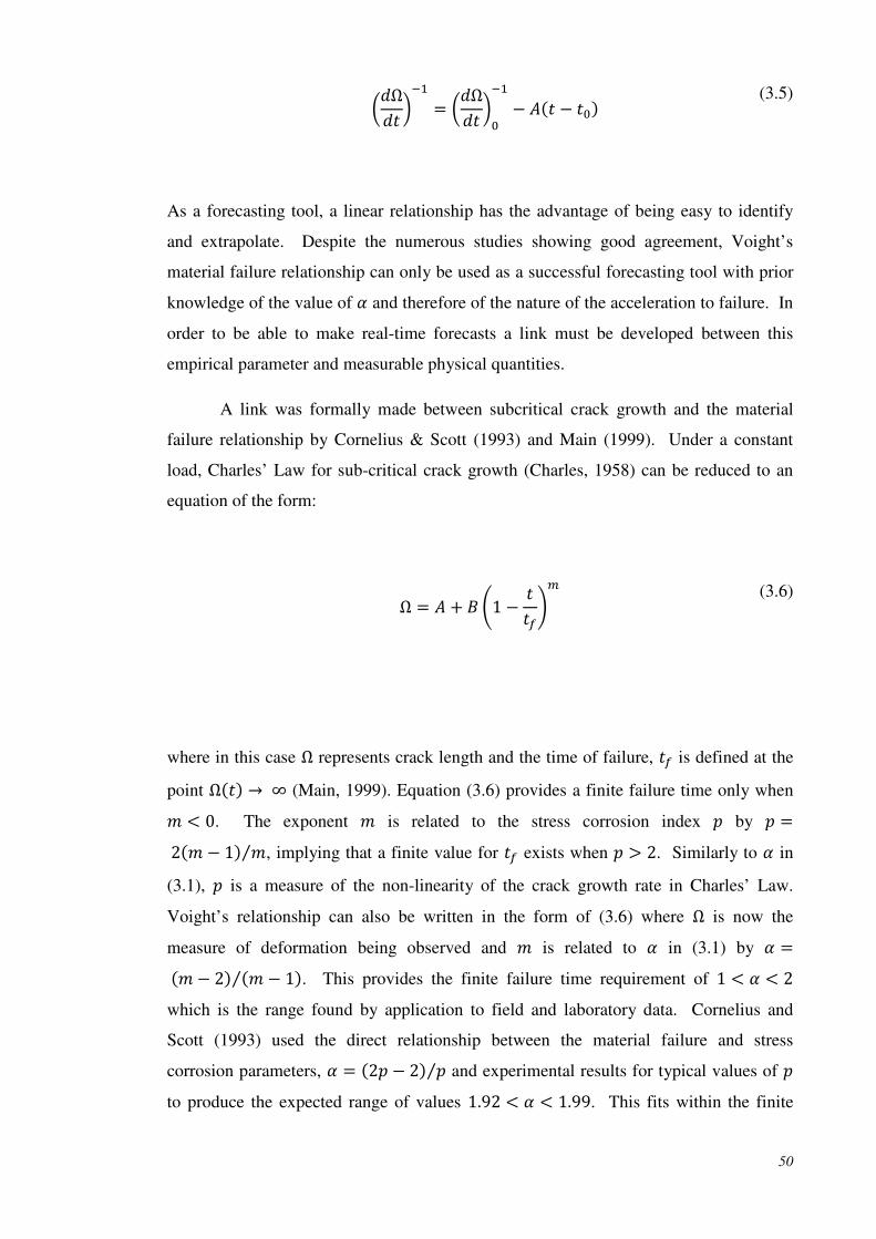
50
/(Ω(@ 0 /(Ω(@ 0" * 6@ * @"7
(3.5)
As a forecasting tool, a linear relationship has the advantage of being easy to identify
and extrapolate. Despite the numerous studies showing good agreement, Voight’s
material failure relationship can only be used as a successful forecasting tool with prior
knowledge of the value of C and therefore of the nature of the acceleration to failure. In
order to be able to make real-time forecasts a link must be developed between this
empirical parameter and measurable physical quantities.
A link was formally made between subcritical crack growth and the material
failure relationship by Cornelius & Scott (1993) and Main (1999). Under a constant
load, Charles’ Law for sub-critical crack growth (Charles, 1958) can be reduced to an
equation of the form:
Ω M N1 * @@EO'
(3.6)
where in this case Ω represents crack length and the time of failure, @E is defined at the
point Ω6@7 P ∞ (Main, 1999). Equation (3.6) provides a finite failure time only when
H 0. The exponent is related to the stress corrosion index R by R 26 * 17 ⁄ , implying that a finite value for @E exists when R 2. Similarly to C in
(3.1), R is a measure of the non-linearity of the crack growth rate in Charles’ Law.
Voight’s relationship can also be written in the form of (3.6) where Ω is now the
measure of deformation being observed and is related to C in (3.1) by C 6 * 27 6 * 17⁄ . This provides the finite failure time requirement of 1 H C H 2
which is the range found by application to field and laboratory data. Cornelius and
Scott (1993) used the direct relationship between the material failure and stress
corrosion parameters, C 62R * 27 R⁄ and experimental results for typical values of R
to produce the expected range of values 1.92 H C H 1.99. This fits within the finite

51
failure time limits and shows good agreement with many of the hind cast applications
(Voight, 1989; Kilburn & Voight, 1998).
Charles’ Law for subcritical crack growth incorporates the stress intensity factor
at the crack tip and therefore relates the empirical quantity C to a theoretical fracture
mechanics process and provides a physical meaning to the parameter. However,
Charles’ Law is still semi-empirical, incorporating an experimentally determined barrier
to crack growth (Cornelius & Scott, 1993). Main (1999) also arrived at an equation of
the form (3.6) describing the non-linear behaviour of the size of connected clusters in a
simple percolation model.
Voight’s failure forecasting relation applied to seismic event rate prior to
eruptions following long repose (Kilburn & Voight, 1998; Kilburn & Sammonds 2005),
finds acceleration parameters consistent with slow fracture under a constant load
(McGuire & Kilburn, 1997), and provides well-constrained forecast windows (Kilburn,
2003; De la Cruz-Reyna & Reyes-Davila, 2001). This method of time-to-failure
analysis is less well defined for non-constant stress or dynamic fracture (Smith et al.,
2007).
All forecasting potential of the material time-to-failure model depends on prior
knowledge of the parameter C and there are very few cases of the material time-to-
failure model being used to issue a real-time forecast (De la Cruz-Reyna & Reyes-
Davila, 2001). Introducing subcritical crack growth relates Voight’s failure forecasting
model to deterministic fracturing laws, however this considers only the growth of a
single, isolated crack. In the heavily fractured crust surrounding a volcano there will be
many cracks, on multiple scales, growing simultaneously. Even under the conditions of
a constant load, proximity of neighbouring fractures will alter the stress field around a
growing crack, to either enhance or diminish the likelihood of further propagation.
Modelling crack growth and failure as an isolated process is therefore discounting a
potentially influential variable in the development of bulk failure.
3.2.2 Multi-scale crack interaction
The failure forecasting relation (3.1) has also been applied to a population of cracks.
Under a constant load the nature of deformation within a fractured body will evolve
from the initial increase of newly active cracks within a fixed volume, to the extension
of a fixed number of active cracks (McGuire & Kilburn, 1997). In terms of Voight’s

52
material failure relation, this corresponds to the acceleration parameter increasing from
C 1 to C 2 as the dominant mode of failure progresses from crack initiation to
crack propagation (Kilburn & Voight, 1998; McGuire & Kilburn, 1997). Growth and
coalescence of fractures will prevail during the final stages of bulk failure and therefore
an increase towards C 2 is expected in the days prior to an eruption.
Kilburn (2003) considered the growth, interaction and coalescence of fractures
on multiple scales, equating a step increase in crack length with a seismic event. The
entire process of growth and coalescence of cracks on one scale can be viewed as the
extension of a crack on a larger scale, which on extending and joining up with
neighbouring cracks will constitute the extension of a fracture on an even greater scale,
and so on. While remaining consistent with Voight’s material failure model, this multi-
scale fracture model forecasts an C 2 acceleration for peak seismic event rate, with
intermediary, non-peak events representing fracturing on a smaller scale. Again
assuming a constant far-field load, Kilburn (2003) considered the role of random energy
fluctuations on a population of multi-scale cracks. A statistical physics approach means
that only the distribution of energy among a population of cracks needs to be
considered, rather than the energy supplied to each individual crack. Following similar
analysis to Boltzmann’s work on the movement of gas molecules (Ruhla, 1992), the
distribution of energy states describes the probability of cracks being supplied with
sufficient energy for propagation. This leads to an expression for the expected rate of
cracking, and therefore seismicity:
((@ S ITU (3.7)
with 4 the extra energy required by crack : for propagation. The rate of cracking is
directly dependent on the energy supplied and following the Boltzmann distribution for
statistical equilibrium (Ruhla, 1992; Kilburn, 2003) there is a much greater probability
of a small amount of energy being supplied than a large amount. From (3.7), as the
energy required for propagation decreases linearly the probability of that energy being
supplied, and therefore the crack rate, increases exponentially.

53
The energy required for crack propagation is the difference between the energy required
to create new crack surfaces and the strain energy released by surrounding rock by the
process of propagation (Griffith, 1920). This can be written in terms of an initial crack
length " and increase in crack length per fracture step ∆ and decreases linearly with
the number of previous fracture steps:
* M "∆ * M (3.8)
where constants and M are functions of the surface energy and strain energy for crack
extension ∆ and total internal energy (Kilburn, 2003). Substituting the above energy
equation into the expected crack rate (3.7) gives Voight’s material failure relation for
the special case of C 2:
((@ S IW (3.9)
The multi-scale fracture model again gives physical reasons for the empirical
laws based on observed patterns before eruptions at long repose volcanoes. Although
this method has never been used in a real time forecasting situation, the model produces
relatively well-constrained forecasts for and is consistent with precursory seismicity to
the eruptions at Pinatubo in 1991 and Soufrière Hills in 1995. As the model itself
predicts a value for the acceleration parameter C, a forecast only requires sufficient data
points to identify a linear inverse trend. The statistical approach requires no detailed
knowledge of the stress field or level of fracture damage in the crust. However, due to
the infrequent occurrence of eruptions at long repose volcanoes, precursory seismic data
prior to these eruptions is very scarce. While the hyperbolic acceleration to failure is
consistent with data sets currently available, there is no way to know if this same trend
is always to be expected or is just one pattern out of many possibilities.

54
Fig. 3.2 (a) Seismic event rate, per 4 hours, prior to the 1991 eruption at Pinatubo. Filled triangles highlight the peaks in event rate, associated with failure on the largest scale in Kilburn’s multiscale fracture model (Kilburn, 2003). The linear trend produced by the inverse of event rate peaks (b) is used to produce a failure forecast time, with failure expected when the trend equals zero. The arrow indicates time of eruption.
Time (Hours from 00.00 June 01, 1991)
Time (Hours from 00.00 June 01, 1991)
Num
ber
of E
vent
s pe
r 4
Hou
rs
Inve
rse
Eve
nt R
ate
(4 H
ours
)

55
Fig. 3.3 (a) Daily seismic event rate prior to the 1995 eruption at Soufrière Hills. Filled triangles highlight the peaks in event rate, associated with failure on the largest scale in Kilburn’s multiscale fracture model (Kilburn, 2003). The linear trend produced by the inverse of event rate peaks (b) is used to produce a failure forecast time, with failure expected when the trend equals zero. The arrow indicates time of eruption.
3.2.3 Propagation and arrest of dykes in a heterogeneous crust
The material failure based models described above predict an acceleration of seismic
activity or fracture length suggesting that the process, once begun is uncontrollable.
Bulk-failure or eruption is inevitable, the only uncertainty being the time of this event.
This runaway style procedure does not explain the occurrence of seismic unrest at
Time (Days from 00.00 November 01, 1995)
Time (Days from 00.00 November 01, 1995)
Num
ber
of S
eism
ic E
vent
s pe
r D
ay
Inve
rse
Eve
nt R
ate
(Day
s)

56
volcanoes or evidence of intruded dykes that never reach the surface (Pinel & Jaupart,
2000). Gudmundsson (2006; 2002) and Gudmundsson and Loetveit (2005) address this
issue with a deterministic view of dyke propagation and arrest.
Gudmundsson and Loetveit (2005) considered dyke injection and dyke fed
eruptions in rift zones and found that mechanically soft layers of pyroclastic material at
shallow depth favour the arrest of propagating dykes. Extensional dyke formation is not
confined to rift zones but can occur even in a compressional setting, where dykes will
form parallel to the maximum and normal to the minimum compressional stresses.
Equally, the action of layers of unfavourable stress conditions acting as barriers to the
propagation of extensional dykes applies in various volcanic settings (Gudmundsson,
2002; Gudmundsson, 2006). However, the successive emplacement of arrested dykes
gradually homogenises the crust between a magma chamber and the surface, making
conditions for eruption more favourable (Gudmundsson, 2002). The relative favouring
of dyke propagation or arrest depends only on the mechanical properties of the host rock
and the necessary conditions for chamber rupture being supplied by the local stress
field, whether this is dominated by the far-field tectonic regime or local effects of
magma-induced loading. This mechanism for dyke arrest should therefore apply equally
well to any volcanic setting (Gudmundsson, 2006). These models consider the
propagation of a magma filled dyke and not the formation and propagation of fractures
due to rock weakening and crack interaction, as addressed in this research. However, it
is instructive to consider the mechanisms proposed for the suppression of a fracturing
process to understand how an accelerating seismic swarm may pass without bulk failure
and eruption. The simulation of a layered material made up of varying critical
toughness is a simple concept to build into a fracture model based on material
properties, and also reproduces an important aspect of a volcanic edifice.
A molten magma chamber can be modelled as a cavity or hole in an elastic solid
that disturbs the remote stress field, such that stress concentrates around the magma
chamber. Analytical models exist for the behaviour of such a magma chamber in a
homogeneous, isotropic crust (Pinel & Jaupart, 2003). Similarly to the runaway, slow
fracturing process, injected dykes in a homogeneous model will meet little resistance
and will generally propagate to the surface (Gudmundsson, 2006). Typically however,
the crust surrounding a magma chamber will be highly heterogeneous and anisotropic
and simple, analytical solutions of stress field perturbation are not accurate. Composite
volcanoes especially, will often be made of alternating layers of stiff lava flows and soft

57
pyroclastic material (Gudmundsson, 2006). Gudmundsson (2006) models the effects of
layering in the crust on the trajectories of principal compressive stresses, which depend
also on the depth, size and geometry of the magma chamber. Boundaries between
layers can cause the trajectory of maximum compressive stress to become horizontal,
favouring dyke arrest over further propagation. This layering is therefore one possible
mechanism to explain the prevalence of injected dykes that never reach the surface.
The dyke propagation model considers only an isolated, magma filled fracture
and the effects of the mechanical properties of host rock on the growth of this fracture.
Just as stress will concentrate around the magma chamber itself, other faults and
fractures within the crust will also alter the local stress field. The magnitude of
magmatic pressure decreases with distance from the magma chamber, and at distances
on the order of the chamber diameter becomes negligible (Gudmundsson, 2006), but
slow fracturing can occur even under a constant load due to rock weakening (McGuire
& Kilburn, 1997). The distribution of pre-eruptive, fracture induced seismicity suggests
scattered failure rather than a purely magma-driven fracturing.
Gudmundsson’s dyke emplacement model and Kilburn’s slow fracture model
need not be mutually exclusive, but can describe the effects of stress concentrations
around cracks, holes or inclusions both immediately surrounding a magma chamber,
and throughout the surrounding host rock. Gudmundsson’s model also predicts the
gradual homogenisation of the crust (Gudmundsson, 2002) and therefore an evolution
towards conditions under which Kilburn’s multi-scale fracture process explains the rock
weakening generated, seismic acceleration to failure and eruption. Gargani et al. (2006)
combine the theories of magma-driven failure and fault interaction. They use Coulomb
stress change in a finite element model to identify the effect of magma-induced stress
perturbations around a molten chamber on pre-existing faults throughout the edifice.
Local stresses may create further fracturing of the host rock that in turn influences the
magma’s pathway from the chamber to the surface. This style of interaction between
local stresses and developing fracture networks is one of the key focuses of this
research. The finite element model produces surface deformation consistent with field
observations, and also indicates regions where seismogenic faulting is most likely to
occur. However Coulomb stress transfer shows only where the probability of, or
proximity to failure has increased or decreased. With a strict failure criterion it is
possible to model directly the formation of a network of fractures and also to
incorporate into the model the effects of material properties.

58
3.3 Fracture mechanics and crack interaction model
In the previous chapter Griffith’s energy balance was seen to provide a necessary
criterion for fracture, while a critical crack tip stress intensity factor was both a
necessary and sufficient condition for crack propagation. The model developed here
will represent the evolution of a fractured rock mass and will require the deterministic
approach of crack tip characterisation, rather than an energy based structure. The aim is
a model based on fundamental fracture mechanics results that will produce an
observable output for forecasting purposes. Gudmundsson’s deterministic model is
based on stress field analysis but offers no observational forecasting tool. An accurate
forecast of dyke propagation and arrest requires detailed knowledge of local loading and
geometrical form of the volcanic system. Voight’s failure forecasting method on the
other hand is developed directly from observations. However, in this case producing a
forecast requires knowledge of, or an assumption of the value for acceleration parameter
C. Kilburn (2003) derived specific values of this parameter that should be expected if
failure occurs by slow, multi-scale fracturing under a constant load, and which is
consistent with observations. This offers a physical explanation of observable
precursors, but has the limitation that it offers no insight into any other mechanisms of
pre-eruptive fracturing (Smith et al., 2007), or into different observations that may occur
in the future.
The prospective approach taken here requires no prior assumption on the style of
fracture rate or acceleration, and therefore places no explicit restriction on the patterns
of fracture rate observed, although implicit restrictions may exist due to the very nature
of the process being modelled. As well as potentially highlighting any alternative
precursory sequences to those that have previously been analysed and modelled, this
may also demonstrate necessary conditions under which particular sequences are
observed. In addition, the model will not be limited to accelerating sequences only and
may therefore be able to reproduce, and hence underline possible causes of seismic
swarms that do not result in bulk failure and eruption. In terms of a recordable
observation, rates of fracturing in the crust can be correlated with high frequency
seismicity, similarly to acoustic emissions measured during fracture experiments in the
laboratory (Lockner et al., 1991). Long period or hybrid events may also represent
fracture processes within a volcano (Tuffen & Dingwell, 2005; Tuffen et al., 2003).
However, these are thought to be produced by fracturing of conduit walls and magma
rather than in the process of edifice failure and conduit formation, and the majority of

59
long period signals are related to the movement of fluids (McNutt, 2005). The bulk of
pre-eruptive, conduit forming failure will occur in the brittle elastic regime and allows
reasonable use of well established linear elastic fracture results.
Fracture mechanisms can be affected by numerous factors such as pressure,
temperature, humidity and material properties. The model produced here will attempt to
capture the most important of these factors on the parameters of interest, namely crack
propagation and coalescence. The mechanical properties of host rock have been shown
to have significant consequences when the same fracture processes have been modelled
in a homogeneous and heterogeneous setting (Gudmundsson, 2006; Liu et al., 2007). A
heterogeneous crust can present stress barriers or areas of weakness that will have a
considerable effect on the growth and coalescence of a population of cracks. The
interaction of cracks on a stressed body has also been highlighted as a crucial element of
failure. Laboratory experiments suggest that coalescence of micro-cracks is the major
process leading to eventual bulk failure of a sample (Amitrano, 2006; Tang, 1997).
Ashby and Hallam (1986) described the significance of crack interaction in the
fracturing and failing of a brittle material loaded in compression. Crack interaction
affects the stress field surrounding close neighbouring cracks and therefore plays an
important role in evaluating crack tip characterisation (Lam & Phua, 1991) and
subcritical crack growth (Kamaya & Totsuka, 2002). As a result, it is important to
consider a population of cracks as a whole rather than just the combined contributions
of each individual fracture.

60
3.4 Chapter summary
Fracture mechanics and failure forecasting have been successfully applied to various
areas of volcanology as well as Earth Sciences as a whole. A model of failure
mechanisms within a volcanic edifice must incorporate variations in material properties
and damage of rock, two important characteristics of individual volcanoes that have a
significant effect on fracturing. Even in the absence of precise data it is possible to
describe the influence of factors such as remotely applied load, crack geometry, crack
interaction and host rock heterogeneity on the development of a fracture network. Both
a constant applied load, assuming rock weakening as the sole controlling factor on
fracture and magma ascent, and a variable remote stress, due to failure related processes
such as deformation or magma degassing can be modelled. Comparison of these results
along with those from different distributions for host rock fracture toughness and initial
crack network geometry can give indication to the relative importance of these variables
on the outcome of a loaded, fractured volcanic edifice.

61
4. One dimensional model of pre-eruptive seismicity
4.1 Introduction
As described in the previous chapter, evidence for fracturing at volcanoes exists in the
form of direct field observations and the development of seismic activity throughout the
surrounding crust. The model developed here is based on failure mechanisms preceding
an eruption at a long repose volcano and therefore assumes a closed system in which
rock weakening is the driving force behind fracturing.
The effects on a volcanic system of rock mechanical properties and the
surrounding stress field are described by a one-dimensional array representing the
progression of failure throughout a volcano. The initial, intact structure is made up of a
number of individual cells, which fail if the local stress intensity exceeds their critical
fracture toughness. Stress intensity is a function of neighbouring crack geometry, as
well as applied stresses. Cells exist in one of two states, either intact or failed, and once
a cell has failed it remains in that state. The number of adjacent failed cells corresponds
to the crack length. A connected network of failed cells, extending through the full
height of the array, represents a fully connected conduit (Fig. 4.1). A one-dimensional
representation is clearly a highly simplified view of the process of crack extension and
interaction. Cracks are unlikely to extend and coalesce in a purely tip-to-tip nature, but
instead will join through the formation of shear cracks between non-aligned sub-vertical
cracks or in some cases will tend to avoid neighbouring cracks leading to arrest of
propagation. For this simplified 1D representation, this process has essentially been
collapsed down to allow failure in one direction only. For the model it is therefore
assumed that cracks will tend to propagate in a tensile mode, in a plane perpendicular to
applied stress. In this representation shear stresses cannot exist. Crack arrest can still
occur within this model, by the propagation of the crack into an area of greater fracture
thoughness.

62
Fig. 4.1 One dimensional array representing a potential pathway to the surface. The array contains a fixed number of cells, each assigned a fracture toughness value. Stress is applied to the array and each cell experinces a stress intensity dependent on the applied stress and location of surrounding cracks. Cells fail once the stress intensity exceeds its fracture toughness. The failure of cells corresponds to seismic events. Grey cells are intact, red cells have failed.
4.2 Physical basis of model
As significant factors in the fracture process, heterogeneous mechanical properties of
the host rock and crack interaction are both incorporated into the model. It is assumed
that conditions controlling micro-fracturing observed in the laboratory can be applied to
macroscopic failure of the scale occurring within the Earth’s crust. Statistics of acoustic
emissions and scaling parameters from laboratory experiments on rock samples show
similarities to those observed in a natural setting. Behaviour of fractures also shows
self-similarity over a range of scales (Lockner & Madden, 1991; Xie, 1993). Therefore
it is assumed reasonable to apply fracture mechanisms at multiple scales.
4.2.1 Fracture toughness
Heterogeneity of the fracture toughness of rock between a magma chamber and the
surface can be introduced into the model using a statistical approach. The Weibull
distribution is widely used for representing the distribution of strengths and lifetimes
(Weibull, 1951; Tang, 1997; Abaimov et al., 2007). The distribution is based on the
concept of a weakest link, and uses the multiplication of the probability of failure of
single elements to model failure of the whole (Weibull, 1951). The basic distribution
function has the form:
Failed
Intact

63
67 1 * I<XY (4.1)
where and . are scale and shape parameters respectively. The Weibull distribution is
an extreme value distribution, with the shape parameter . controlling the tail of the
distribution. Its utility also stems from its flexibility. The Weibull distribution
approximates a normal distribution when the parameter . 3.4, and reduces to an
exponential distribution when . 1.
Although the strength and toughness of a material are two different parameters,
under various distributions, including Weibull, they may both be described by the same
statistical distribution (Xing et al., 1993; Emmerich, 2007). However, it has been
suggested that the theoretical basis for the use of the Weibull distribution no longer
holds when considering a material’s resistance to crack propagation, and that fracture
toughness data exhibits a systematic deviation from what is otherwise a reasonable fit
by the distribution (Neville & Knott, 1986). Neville (1987) suggests an alternative
distribution, based on the theory of stress concentration at crack tips:
6[7 6[ M⁄ 7\1 6[ M⁄ 7\
(4.2)
“Sampling” [ is defined as a power of the stress intensity factor, [ 3], M is the scale
parameter and is the shape parameter. Hazzard et al. (2000) assign bond strengths
following a Gaussian distribution in their micromechanical rock failure model, using the
variance to control the degree of heterogeneity. Due to its flexibility a Weibull
distribution is used to assign cell fracture toughness in the one-dimensional model. By
varied selection of parameters, alternative proposed distributions, such as Gaussian can
also be accounted for.
Spatial distribution and variability of fracture toughness must also be
considered, as along with the statistical distribution, they determine the degree of
heterogeneity in the model. A random spatial design can be achieved through a random
walk process. A random walk is a sequence of discrete steps, with the magnitude and
direction of each step being selected at random from the specified distribution.

64
Henderson and Main (1992) refer to the abundance of examples of random walks in
nature and assign toughness values to their fracture model using a random walk on a
Gaussian distribution. A layered structure can represent heterogeneous strata making up
a volcanic edifice whilst assuming broad homogeneity of mechanical properties within
these strata (Gudmundsson, 2005). For any statistical distribution selected, appropriate
experimental data can provide suitable range limits or scale parameter values. In the
one-dimensional model both random and layered distributions are applied.
Experimental data exists for fracture toughness measurements over a variety of
temperature and pressure conditions for both intrusive and extrusive rock. Meredith and
Atkinson (1985) measured the fracture toughness for intrusive rocks, at temperatures
from 20 to 400°C and found values between 1.7 and 3.1 MPa√m for Westerly granite
and Black gabbro. Balme et al (2004) conducted high-pressure and high-temperature
experiments on Icelandic, Vesuvian and Etnean basalts and measured fracture toughness
values between 1.4 and 3.8 MPa√m. In laboratory experiments, Smith (2007) measured
fracture toughness at pressure and temperature conditions consistent with different
regions within a volcano, including material close to a conduit, close to a magma
source, and rock at depths of 1.5-2.5 km beneath the summit of a volcano. Experiments
were carried out on ancestral Mt Shasta andesite and over the various conditions the
fracture toughness measured remained consistent around 2.5±0.5 MPa√m.
4.2.2 Flaw distribution
Applied stress will concentrate at crack tips and therefore the number, location and size
of initial cracks will also affect the progression of the model. In assigning a geometry
for initial flaws, both crack length distribution and crack density must be considered.
Steacy and Sammis (1992) assume a fractal distribution for starter flaws in their damage
mechanics model. Under this assumption, crack size frequency will follow a power law
relation between limits of a maximum and a minimum flaw size, where the latter may
be dependent on the observation scale, and for modelling will be limited by grid size.
Power law trends have been found for crack length populations from the laboratory
scale to the field scale (Wong et al., 2006; Hatton et al., 1993).
Renshaw and Pollard (1994) use a uniform probability distribution to assign
initial flaw geometry in their numerical fracture set model. Altering the critical
probability value in their model, above which a network node fails, creates different

65
starting distributions. On comparison of the numerical fracture sets with experimental
results, “invisible” flaws were added to the numerical distribution to allow for the
growth of cracks initially smaller than the model grid size. In the model presented here,
the initial location of cracks or flaws can be related to the specified fracture toughness
distribution. Fracture toughness measures resistance to propagation of an existing crack
and therefore a low value of this property at the grid scale can be associated with the
presence of a microcrack at the smaller, invisible scale. In other words, as soon as
stress is applied to the model, the weakest areas will fail first, producing an initial
distribution of cracks in a similar fashion to the critical probability threshold described
above. The spatial and statistical distributions of fracture toughness can then also
control the initial crack length statistics.
The pre-existing distribution of flaws or cracks within the crust is highly
heterogeneous, depending greatly on the rock and stress history (Wong et al., 2006;
Kranz, 1983). Even in the case of a long repose volcano, host rock within and below a
volcanic edifice may be heavily fractured (Kilburn, 2003; Scandone et al., 2007) and it
will therefore be instructive to also consider the effects of larger scale faults and cracks
within an interacting fracture network.
4.2.3 Stress field
In addition to the regional stress field within which a volcano lies, the local stress field
can also be affected by topographic loading, and magma and hydrothermal processes
(Roman et al., 2004). Topographic loading of the crust has been identified as a major
influence on the stress field and resulting seismicity at Mt. Spurr, Alaska and Mt.
Vesuvius, Italy (Jolly et al., 1994; De Natale et al., 2000). Roman et al. have looked at
the evolution of local stress fields both before and during eruptions at Mt. Spurr (2004)
and episodes during the ongoing activity at Soufrière Hills, Montserrat (2008), using
detailed analysis of seismic data. Analysis of fault plane solutions of VT events in the
weeks to days prior to renewed activity at Soufrière Hills, suggests that the local stress-
field undergoes a 90° reorientation during this period. This is correlated with the
inflation of a dyke located beneath the vent, and is proposed as a forecasting tool for
future activity. However, few sufficiently detailed earthquake data sets exist to enable
this method to be used to provide a general picture of local stress fields within a
volcano.
66
Experimental data is largely produced under constant strain rate or constant load
testing, modelling rock deformation response to either a regional strain or fixed stress
field (e.g. Mavko et al., 1998). The influence of both constant and variable stress
conditions on the development of fracture networks has been highlighted by numerical
models (Renshaw & Pollard, 1994; Tuckwell, 2003), and fracture patterns in geological
materials can be used to interpret the local stress history. In particular, failure of the
crust has been modelled under both constant and increasing stresses. Modelling
earthquake recurrence times, Main (1988) considered a time dependent remote stress
with a constant load rate :
6@7 " @ (4.3)
De la Cruz-Reyna and Reyes-Davila (2001) developed a visco-elastic model for
material failure, with applications to eruption forecasting, and considered a constant
load, a linearly increasing load, and an initially increasing load which is then held
constant at " after time @<:
6@7 "@< @a6@< * @7 "a6@ * @<7 (4.4)
Non-linear increases in stress have generally been associated with magma induced
pressure changes, for example in relation to lava-dome eruptions (Sparks, 1997).
The time scale involved when considering medium-term precursory activity is
relatively short compared with that for magma induced pressure changes. The lack of
migration of VT seismicity prior to eruption suggests that magma intrusion is not a
source of stress variation during this process. Slow rock fracture as a control on magma
ascent also requires no magma generated increase in pressure (Kilburn & Voight, 1998).
Therefore in the one-dimensional model of precursory fracture, an assumption of a
temporally constant local stress field is also a reasonable model parameter.
67
4.2.4 Stress intensity
Stress applied to a body will concentrate at the tips of cracks and flaws within the
material, as described in Chapter 2. The remote stress applied to the model is adjusted
locally according to the geometry of surrounding cracks. For an isolated, two-
dimensional crack the stress intensity factor at each of its tip is given by:
3 √+ (4.5)
where is the crack semi-length and the applied stress (Lawn & Wilshaw, 1975). In
the crack tip region, stresses decrease with the inverse square root of distance from the
crack tip (Atkinson, 1987). The stress intensity factor deals with the magnitude of
crack-tip stress concentration and the likelihood of a fracture to propagate. Here it is
also assumed that the stress intensity factor determines the extent of crack propagation.
The greater the crack length, the greater the degree of stress concentration, and the
greater the expected increase in crack length (Tuckwell et al., 2003). The crack-tip
stress intensity is reduced with distance from the crack, within the range of half the
crack length. The extent of propagation will then depend on both crack length and local
fracture toughness, with failure occurring a distance from an isolated crack if local
toughness is exceeded by:
3 b+ (4.6)
As cracks form closer together they will interact mechanically and therefore no longer
act as isolated cracks. Tuckwell et al. (2003) allow for crack interaction by defining a
non-linear process zone around propagating crack tips, the extent of which is dependent
on the crack tip stress intensity. Neighbouring cracks will join up if their respective
process zones overlap. This method allows only for the coalescence of cracks due to
mechanical interaction and not individual crack growth as a result of stress intensity
increase in the presence of a neighbouring crack (Sammonds & Ohnaka, 1998).
Kachanov (1987) proposes a superposition technique for approximating linear elastic
stress fields surrounding an arbitrary distribution of cracks. The integral based

68
technique produces good approximations to known analytical results until the distance
between cracks becomes small relative to crack length, in which case the effects of
crack interaction are underestimated.
Fig. 4.2 Crack length and spacing measurements used in Rudnicki and Kanamori’s stress intensity calculations for an infinite array.
Analytical solutions for crack-tip stress fields exist for only a small number of,
generally uniform, geometries of neighbouring, interacting cracks (Tada et al., 1973).
As described by Rudnicki and Kanamori (1981), the crack-tip stress intensity factor for an
infinite periodic array of cracks is:
3 c tan g+ hi ⁄
(4.7)
where is the distance from one crack centre to the next (Fig. 4.2). When cracks are a
great enough distance apart to behave as isolated cracks, Equation (4.7) reduces to (4.6)
by the property tan 9 j 9 for small values of 9. Following Henderson and Main (1992),
the effects of crack interaction on stress intensity at crack tips and the region between
neighbouring cracks is assigned using Equation (4.7), adjusted to allow for unequal
crack lengths and inter-crack distances. For a cell in the one-dimensional array, a
distance and respectively from adjacent cracks of length 2 and 2, the stress
intensity is calculated by summing the effects of each crack interacting with a notional
crack of the same size. This sum is adjusted by a factor dependent on the crack lengths
24 and the point’s distance from each crack 4, also allowing for attenuation of the
concentration away from crack-tips:

69
3 8k4, 4m n o4 tan /+44 0p ⁄4q,
(4.8)
8 1 r1 * 45s 45t5 (4.9)
is the actual centre to centre distance, while 4 represents the centre to centre distance
between crack : and the notional crack of the same length (Fig. 4.3). 45 is the
Kronecker delta function.
Fig. 4.3 The stress intensity at a distance from a crack of length 2, and distance from a crack of length 2 (top), is calculated by summing the effects of each of the two cracks interacting with a notional crack of equal length (grey cracks), as described in Equation (4.8). The distance between the modeled and notional cracks is the same as that between the original cracks (i.e. ). The centre-to-centre distances between the two modeled cracks and the modeled and notional cracks are given by , and respectively, and are related by 2 .
Again, this term for stress intensity concentration tends back to (4.6) when the inter-
crack distance is large. For example, when two identical cracks are separated by a
distance equal to their length, the effect of interaction on the crack tips increases the
stress intensity by just 10% (Rudnicki & Kanamori, 1981).

70
This interaction effect creates a positive feedback process. As cracks form close
together the surrounding stress intensity is increased, causing new cracks to form, which
further increases the stress; thus, under certain conditions, a runaway fracturing process
is established, and the system rapidly runs to failure.

71
4.3 Description of model
4.3.1 Initial conditions
In the one dimensional array, a fully connected pathway can arise only when all cells
have failed. Model sizes up to 7,000 cells were tested. Results remained statistically
consistent for sizes above 1,000 cells and therefore model sizes of 1,000 - 2,000 cells
were generally used, in order to reduce long computational running times.
Following the discussion in Section 4.2.1, a fracture toughness value is assigned
to each cell by generating a random walk on a Weibull distribution. Initially the shape
parameter of the Weibull distribution has a normal distribution with mean 3.4. Values
are arranged spatially according to the number of homogeneous layers to be modelled,
and the degree of local homogeneity within these layers. For example, for complete
heterogeneity a number of layers equal to the number of cells can be selected. The
series of fracture toughness values produced by the random walk process are sorted into
ascending order and distributed over the cells according to the number of layers and
homogeneity within each layer. For a homogeneous layer, consecutive values from the
ordered list are selected. For a layer with a greater degree of heterongeneity, values are
selected from a larger range within the list of toughness values.
As described in Section 4.2.2, flaws are naturally introduced into the array when
the initial stress is applied and cells with a fracture toughness value less than the applied
stress fail immediately. For model runs where a specified distribution of flaws is being
tested, for example a set of cracks with a power law frequency-length distribution, this
distribution is then also assigned. If a greater number of initial flaws are required than
those that naturally fail due their fracture toughness, these extra flaws are added by
randomly selecting intact cells and assigning a state of failure. Table 4.1 contains each
of the input parameters and their respective ranges.

72
Input parameter Distribution/Range
Fracture toughness Weibullk, um ~ N [3.4, 1], u ~ N [1, 1]
Number of layers for fracture
toughness homogeneity
R [1, w] (w = number of cells)
Homogeneity within layers R[0, 1] (a value of 0 implies toughness values are
assigned at random within the layer, a value of 1
implies toughness values are assigned in numerical
order within the layer.
Number of initial flaws R[0, w/50] (w = number of cells)
Table 4.1 Distributions for input parameters to the one-dimensional model.
4.3.2 Running the model
An initial stress is applied uniformly to the model and a stress intensity value is
calculated for each cell, dependent on the geometry of neighbouring flaws, by Equations
(4.6) and (4.8). After checking for failing cells the stress intensity values are then re-
calculated, taking into account any newly failed cells and adjustment of the remote
stress level. Cells are then again checked for failure. These iterations continue until
either all cells have failed and a connected pathway is formed, or until no further
failures will occur under the prescribed loading conditions. The model is generally run
under one of two conditions: constant stress or constant load rate.
Under constant stress, the remotely applied stress remains the same during each
iteration of the model and changes to stress intensity arise solely due to the failure of
new cells. The model need not always fail under this condition, but can instead reach a
state of stability where no further cells are caused to fail. To simulate a constant load
rate, some measure of time must be introduced into the model. Each iteration in the
running of the model provides a natural measurement of time, as the static stress
transfer involved can generally be assumed to occur on a time-scale independent of the
size or location of the failure event. A constant load rate is therefore modelled by a
regular increase in the remote stress with each iteration of the model.

73
4.3.3 Seismic event rate
The failure of a cell is considered as representing a seismic event and the event rate is
therefore simply the number of cells failing during each iteration of the model. This is
recorded along with the location of events, to enable a picture of the spatial
development of cracks. An approximate magnitude of events is measured by the length
x of adjacent cells failing simultaneously, via a logarithmic relation:
4 * w log x (4.10)
The constant w takes a value between 3 and 4 (Kanamori & Anderson, 1975) and is
selected to scale the magnitude. For example, if w 4 and 10 the failure of a
single isolated cell will produce a magnitude zero event. If w 3, 10 results in a
single failure producing a magnitude one event.
By altering the initial variables in the model it is possible to investigate the
effects of mechanical inhomogeneities, the extent of damage, and the local stress
conditions on the development of a fracture network.

74
4.4 Observations and sensitivity analysis
4.4.1 Exponential acceleration and linear inverse trend
When run under constant stress or constant load rate, with input parameters taken
randomly from the distributions described in Table 4.1, the prevailing patterns of
seismic event rate observed are comprised of exponential increase with time, and linear
inverse event rate with time. A linear inverse rate can be extrapolated towards a
singularity point of infinite event rate and describes hyperbolic growth. A continuous
exponential growth or an initial exponential growth that becomes hyperbolic prior to
failure, are patterns observed in the model. Representative results are shown in this
section, and are typical of the output distibutions produced by random simulations of
the one-dimensional model. Figure 4.4 contains two examples of model outputs,
showing a good fit ( 0.9) to each of these growth patterns respectively. Figure 4.5
shows the progression of the array for each example.
A drop-off in the event rate is often seen immediately prior to failure. In the
case where this coincides with the time of failure, as in the example in Figure 4.4a, it is
assumed that this is due to the closed nature of a one dimensional model. During the
final loop of the process, there will be a limited number of cells that remain intact and
are subsequently available to fail and produce a seismic event.

75
(a)
(b)
Fig. 4.4 Typical outputs from the one dimensional model under a constant stress, showing seismic event rate with time. (a) Exponential growth is often recorded. Inset shows the natural log of event rate, with a good linear fit ( 0.99). A drop-off in event rate is often seen immediately prior to failure due to a limited number of cells remaining intact. (b) A trend which becomes hyperbolic is also observed. Inset shows the initial linear log event rate ( 0.99), followed by a linear inverse rate, signifying the onset of hyperbolic growth ( 0.99).
Eve
nts
Time
Eve
nts
Time

76
Fig. 4.5 Progression of the one dimensional array with time. Intact cells are grey, failed cells red. (a) Failure dominated by one primary fracture produced the exponential trend in seismicity shown in Fig. 4.4a. (b) Event rate produced is exponential initially, but becomes hyperbolic prior to failure (Fig. 4.4b). Results represent typical examples from multiple runs of the model.
Figure 4.6 shows an additional example of the progression of the model array,
and the resulting linear inverse event rate. In this particular case a greater number of
primary cracks grow throughout the model, allowing for greater crack interaction
effects.
Intact
Time
Failed
a) b)

77
Fig. 4.6 Progression of one-dimensional array with time, showing simultaneous growth and interaction of multiple cracks, and the resulting event-rate and inverse-rate trends. This represents a typical such result from multiple runs of the model.
4.4.2 Effect of fracture distribution
To gain some understanding of the influence or importance of the distribution of initial
cracks on the evolution of failure, the model was run three times, with the same
distribution of fracture toughness but different arrangements of initial cracks. In each
case 20 out of 1,000 cells were assigned a starting state of failure. In each of the three
cases, these 20 cells were arranged as 10 uniformly separated cracks of length two, one
single, central crack of length 20, and completely at random throughout the array.
When subjected to a uniform load each case produced a seismic event rate with a good
fit to an exponential curve ( 0.94). The magnitude of the applied stress was
Intact
Failed
Time Time

78
chosen to be the minimum value that would lead to complete failure. The rate of
exponential growth was slower in the case with one single crack, with a rate constant of
0.16, compared to values of 0.31 and 0.25 in the uniform and random case respectively.
This may be due to the activity being driven by the growth of a single crack. If multiple
cracks exist, interaction between these cracks further increases stress intensity, and the
coalescence of cracks provides a mechanism for rapid crack growth.
Despite cells having the same fracture toughness value in all three cases,
extensive failure initiates in different regions in each run (Fig. 4.7), implying that low
fracture toughness alone does not determine which areas will fail most readily. The
location of fractures is also important in determining the evolution of a fracture
network.
Fig. 4.7 Progression of cracks with time for three simulations of the one-dimensional model, with identical fracture toughness distribution. Each run has 20 initially failed cells, with a different spatial distribution of the failed cells in each case. (a) Failed cells are
Failed Intact
Time

79
distributed uniformally along the array, as 10 cracks of length 2 with an inter-crack distance of 98 cells. (b) Failed cells produce one single, central crack of length 20. (c) Failed cells are distributed at random along the array.
4.4.3 Effect of fracture toughness distribution
Given uniform fracture toughness, the event rate will be controlled by the stress
intensity distribution and the location of initial cracks. Aside from interaction effects,
two cracks of the same length will extend at the same rate. Under a constant load, the
model will fail if the remotely applied stress is greater than that necessary to cause the
largest crack to extend, as there will be no region of greater fracture toughness to halt
crack growth. This crack, or multiple cracks if there are several of the same length, can
then freely extend throughout the entire array (Fig. 4.8).
Fig. 4.8 Progression of a one dimensional array with uniform fracture toughness. The largest initial crack dominates activity entirely and growth spreads evenly while the model boundaries allow. Growth rate slows slightly once the dominating crack can grow in one direction only.
Failed Intact
Time

80
Under uniform fracture toughness, the model again provides a good fit to
exponential growth in seismic event rate. When the model is run with the same initial
cracks and the minimum stress that produces failure, but with an entirely random
fracture toughness, exponential growth is still observed but the rate constant is generally
lower, with exact magnitudes dependent on the distribution. In other words, the
variable fracture toughness acts to slow down the process somewhat. Once a variable
fracture toughness is introduced, rather than the pure extension of existing cracks,
cracks tend to grow by the development of smaller cracks around its tip, which then
coalesce to create extension of the original crack. This process leads to a damage zone
around an advancing fracture.

81
Fig. 4.9 Event rate and log event rate with time for four runs of the model with an identical distribution of initial flaws, and fracture toughness values assigned from different distributions. Fracture toughness values are selected at random from a rectangular distribution with a range of (a) 5 (b) 20 and (c) 10 units. Values are assigned randomly along the array. (d) The final run has toughness values selected at random from a rectangular distribution with a range of 20 units, which are applied to the array with clusters of similar magnitude values. All runs produce a roughly exponential increase in event rate. The exponential rate constant reduces with the increase in range of the fracture toughness distribution, λ = 0.4, 0.24, 0.28 respectively for ranges 5, 20 and 10 (Figs. (a) to (c)) respectively. A clustered distribution produced the rate λ = 0.39. For the case of a constant fracture toughness (Fig. 4.8) λ = 0.57.
Time
4 8 12
Eve
nts ln
(Eve
nts)
300
200
100
300
200
100
10 20 30
ln(E
vent
s)
300
200
Eve
nts
100
5 10 15 20
ln(E
vent
s)
Eve
nts
300
200
100
ln(E
vent
s)
Eve
nts
6 12 18
(a)
(b)
(c)
(d)

82
The effect of the degree of variability in fracture toughness can also be
considered. The model was run four times, each time with the same initial failures and
the minimum load necessary to ensure failure. A random fracture toughness
distribution is assigned with a range of 5, 10 and 20 units for the first three runs
respectively. Values are selected from a rectangular distribution with ranges described
above. These values are then distributed randomly over the cells. All three distributions
are centred about the same mean, and the increase in range equates to over a 400%
increase in the standard deviation from 1.4 to 5.8. As the variability increases, the
exponential rate constant decreases (Fig. 4.9). For the final run of the model, a
variability range of 20 is again used, but the values are clustered spatially. For example,
cells with a high fracture toughness are more likely to be surrounded by other cells with
a high fracture toughness. This has the effect of increasing the exponential rate of
growth.
4.4.4 Monte Carlo sampling
The range of outputs from the model can be seen to be simultaneously dependent on the
distribution of fractures, the distribution and variability of fracture toughness and the
loading conditions. A Monte Carlo method was used to explore the outcomes of
repeated samplings for combinations of these factors. Clearly a large degree of
uncertainty exists concerning the appropriate inputs to use for any specific volcano
under study. A Monte Carlo simulation provides not only a useful means of assessing
how a variety of conditions may affect seismic event rate, but also the range of
observations which might be expected prior to an eruption.
A separate simulation was run for constant load and constant load rate as the
disparate time scales for these conditions makes comparison difficult. In each case, the
model was run numerous times with different initial conditions chosen at random for
each separate run. The variables selected are the shape and scale parameters used to
describe the Weibull distribution of the fracture toughness values; the number,
respective size and variability of layers for the fracture toughness values; and the
number, length-frequency distribution and the degree of randomness or uniformity to
the location of initially failed cells.

83
Fig. 4.10 Event rate with time for 200 individual runs of the one dimensional model under increasing stress. Input parameters are chosen at random from the distributions described in Table 4.1. Time is measured from the start of each model run.
Under constant loading rate, the same stress increase of 0.1 MPa/unit time was
used in 200 separate runs (Fig. 4.10). This was a value found to be generally large
enough to induce further fracturing, but sufficiently small to allow gradual rather than
large scale failure. Of 200 outputs, 138 showed a significant fit ( 0.9) to a
continuous exponential trend and 4 produced a better fit to an exponential growth that
became hyperbolic prior to failure. The exponential rate constants and inverse gradients
for these observations were also recorded (Fig. 4.11). The exponential constants range
from 0.24 to 3.38, with approximately 80% of the trends having a rate constant less than
0.8. The 4 trends showing hyperbolic growth have inverse gradients of 62.0, 4.17 |10.
Time
Eve
nts

84
Fig. 4.11 Cumulative probability function for (a) the exponential rate constants from 138 Monte Carlo runs producing an expoential increase in event rate, and (b) the gradient of inverse seismic event rate for the 4 Monte Carlo runs producing an exponential followed by hyperbolic increase in event rate. The peak event distributions describe the exponential rate constants and inverse gradients for the Monte Carlo runs when only the local peaks in event rate were used in analysis, as described in Section 3.2.2. When only peak events are included, 29 of the Monte Carlo runs produce an exponential event rate that becomes hyperbolic prior to failure (b), and 7 produce a purely hyperbolic increase. Figure (c) shows the cumulative probability function for the gradient of the inverse event rate in these 7 cases. Event rate trends are the output from 200 individual runs of the one dimensional model subjected to increasing stress.
Many of the observed event rate patterns show an overall exponential or hyperbolic
growth, but due to a greater degree or variability within this trend do not give a
statistically significant fit. To look at the extent of these general trends, a similar
analysis was done for the peak event rates only. Kilburn (2003) demonstrated that the
failure forecast method could be applied to activity occurring on different scales at
Pinatubo and Soufrière Hills. Using only peaks in the model event rate, the 200 runs
produce 133 continuous exponential trends, 29 exponential to hyperbolic trends and 7
Exponential rate constant (λ)
Inverse Gradient b
Inverse Gradient b
P(I
nver
se G
radi
ent <
b)
P(R
ate
Con
stan
t < λ
)
P(I
nver
se G
radi
ent <
b)

85
showing just the hyperbolic section of growth. Exponential rate constants are similarly
distributed as in the case of all events. However, inverse gradients for the purely
hyperbolic growth are in general an order of magnitude greater than those trends that
become hyperbolic following an exponential increase. These purely hyperbolic cases
are, by definition, examples which show rapid growth immediately and this is likely to
occur when the selection of parameters gives relatively homogeneous and low fracture
toughness values. Combined with a distribution of initial flaws that optimises
interaction, this will lead to very rapid bulk failure, with little to slow the process. The
small number of such cases in the simulation suggests that this combination of factors is
statistically uncommon.
Fig. 4.12 Event rate with time for 100 individual runs of the one dimensional model under constant load. Input parameters are chosen at random from a range of possible values and distributions. Time is measured from the start of each model run.
Figure 4.12 shows the results of 100 runs of the model under constant load,
where the level of stress chosen was the minimum required to produce complete failure.
The average failure time under constant stress is longer than that with increasing stress.
Stress intensity is an increasing function of crack length, proximity to a crack and also
external stress. With all factors equal, an array that is subjected to a higher applied
stress will fail more rapidly than that subjected to a lower stress. From the 100 runs,
there were 77 significant ( 0.9) continuous exponential trends, and 9 that became
Time
Eve
nts

86
hyperbolic after an initial exponential increase. The number of significant exponential
to hyperbolic trends increased to 27 when only peak events were considered, with 71
following continuous exponential growth. Exponential rate constants are significantly
lower on average than for the increasing stress case, with values in the range of 0.03 to
0.7 (Fig. 4.13a). Inverse gradients have a similar lower limit to the increasing stress
case, but increase to a lesser maximum of 2.0 | 10 (Fig. 4.13b), again with the peak
event cases showing a wider range of values.
Looking directly at the initial conditions for the different runs, those that
produce an exponential developing into hyperbolic trend appear to have a generally
more homogeneous fracture toughness distribution, and initial flaws that are more
clustered. As described in Section 4.2.1, the shape parameter u of the Weibull
distribution controls the shape of distribution. The mean value for this parameter from
the Monte Carlo runs producing an exponential trend was 1.7. For the exponential to
hyperbolic trends the mean value was 0.8. Lower values of u produce a distribution
closer to an exponential distribution, with a smaller range, and therefore more similar
values than a normal distribution, which is more closely resembled with larger values of
u. Both the exponential and exponential to hyperbolic trends had similar initial
conditions in terms of crack length distribution, with average mean lengths of 1.5 and
1.4 respectively. However, a greater difference was observed in the initial inter-crack
distance distribution. A mean value of 134 was recorded for the runs producing
exponential trends, and 94 for those that progressed into hyperbolic trends.

87
Fig. 4.13 Cumulative probability function for (a) the exponential rate constant from the 77 Monte Carlo runs producing an exponential increase in event rate prior to failure, and (b) the gradient of inverse number of events with time for the 9 Monte Carlo runs producing an exponential trend that becomes hyperbolic prior to failure. The peak event distributions describe the exponential rate constants and inverse gradients for the Monte Carlo runs when only the local peaks in event rate were used in analysis, as described in Section 3.2.2. When only peak events are included, 27 of the Monte Carlo runs produce an exponential event rate that becomes hyperbolic prior to failure (b). Event rate trends are the output from 100 individual runs of the one dimensional model under constant load.
These two types of trend, namely exponential and exponential to hyperbolic,
clearly provide a good description for the majority of outputs from the one dimensional
model, especially when run under a constant stress. In the constant load simulation they
account for 86% of outputs, rising to 98% when only peak events are considered,
compared to values of 71% and 85% respectively when run under an increasing stress.
These two trends are discussed in more detail in Chapter 5. Figure 4.14 shows two
examples of typical alternative outputs that do not fit either of these trends. Some such
outputs show a marked increase in event rate leading up to failure, but a long tail of
Exponential Rate Constant (λ)
Inverse Gradient b

88
much steadier increase prior to this prevents the growth from being described as
exponential or hyperbolic (Fig. 4.14a). Another relatively common pattern is periods of
exponential growth within a more disordered overall trend (Fig. 4.14b).
Fig. 4.14 Examples of alternative event rate trends, produced by the Monte Carlo run, which do not show an exponential or hyperbolic growth.
For completeness, a sampling of 550 runs where loading conditions also differed
was performed (Fig. 4.15). Within each run of the model, the time between successive
stress changes, and the extent of that change was non-uniform. However, to ensure that
the model would always eventually progress to failure, no negative stress changes were
applied. The time scale of failure covers a large range, with some cases in which arrays
failed almost instantly and therefore with very high event rate, or a much longer failure
time associated with a lower general event rate. However, even in these longer, drawn
out trends some degree of increase in event rate can still be seen prior to failure. These
Time
Eve
nts
Eve
nts

89
two extremes in output data may be due to the coupling of relatively homogeneous
fracture toughness and a significant increase in stress for early, rapid failure, and diverse
fracture toughness under a constant or very steadily increasing load, leading to the more
gradual development of failure. The model has the same number of cells in each run
and therefore in general, the shorter failure times will be associated with the larger event
rates.
Fig. 4.15 Event rate with time for 550 individual runs of the one dimensional model. Varying input parameters are fracture toughness and initial flaw distributions, as well as external loading conditions.
Time
Eve
nts

90
4.5 Chapter summary
The one-dimensional model is based on physical principles of the concentration of
stress due to the presence of cracks in a material. Mechanical properties of the host
rock making up a volcanic edifice can be varied within the model, as well as the
surrounding stress field. The distribution of initial cracks in the array, and the
variability of fracture toughness of cells, both affect the failure rate of the model. The
model produces exponential accelerations of failure rate, which in some cases become
hyperbolic prior to bulk failure of the array. A Monte Carlo simulation highlights the
relative probability of each style of precursor as well as providing a possible range of
parameter values.

91
5. Analysis and discussion from 1D model: Accelerations of
seismicity
5.1 Introduction
The Monte Carlo simulation described in the previous chapter showed that, when run
from a suitable range of initial conditions, the one dimensional model will produce a
definite, quantifiable pattern of precursory events. This chapter will consider in more
detail the two predominant trends identified, exponential and hyperbolic, and the
processes that may be responsible for these trends. The precursory sequences are
consistent with the material failure forecast model (Voight, 1988) and crack interaction
model (Kilburn and Voight, 1998) described in Chapter 3, as well as field data and
laboratory observations.
Exponential rates of failure are commonly observed at volcanoes (e.g. Bell,
2008; Kilburn, 2003), and also in compression tests in the laboratory (e.g. Meredith et
al., 1990). In addition, for both field and laboratory data, the emergence of subsequent
faster than exponential trends have also been observed. Field observations from
subduction zone volcanoes show a hyperbolic acceleration in seismicity in the final
weeks prior to eruption (e.g. Kilburn & Voight, 1998; Kilburn, 2003). Tests in the
laboratory show step increases in acoustic emission rates immediately prior to failure
(Meredith et al., 1990). Similarly, the most common trend emerging from the one-
dimensional model is an exponential rate of failure. Under certain conditions, this
exponential trend then switches to become hyperbolic before bulk failure of the array.
In the following sections the exponential and hyperbolic sequences produced by
the one-dimensional model are analysed in an attempt to understand further the
processes creating these particular styles of precursory activity, and the emergence of a
faster than exponential sequence. Aspects of the precursory trend such as duration and
rate are considered, as well as the mechanisms and properties of failure and crack
growth creating the trends.
In the remainder of this chapter, precursory trends produced by the model that
remain exponential to failure are described as Type I trends. Exponential sequences that
become hyperbolic prior to failure are described as Type II trends. Representative
examples of each of these cases are used to illustrate the various analyses described in
the chapter.

92
5.2 Controls on seismic event rate: constraints from field data
Predominantly exponential increases in seismic event rate (Type I) have been observed
weeks to months before magmatic events at basaltic volcanoes, notably at Kilauea and
Mauna Loa, Hawaii, and at Mt. Etna in Italy (Bell, 2007). Intrusive events at the same
volcanoes have shown similar exponential seismic precursors (Bell, 2007), a feature that
will be discussed in Chapter 8. In both cases, any faster-than-exponential trends appear
as step-like increases in seismic event rate that continue for about a day or less.
More generally, exponential trends are observed in many natural processes that
evolve through a mechanism of self-propagation. Applied to fracture growth, self-
propagation is favoured because the stress intensity ahead of a crack increases with
crack length. Thus, as a crack grows, the stress intensity at its tips becomes
progressively larger, so favouring further growth. Once a crack begins to extend,
therefore, the positive feedback between crack length and stress intensity will encourage
an accelerating rate of growth. This behaviour may be altered by interactions with other
cracks, or by the extending crack entering a region of unbroken material with
mechanical properties, such as toughness, that vary significantly from those of the
material through which the crack has just propagated. Such conditions may operate to
increase (e.g., entrance into weaker rock) or to decrease (e.g., entrance into stronger
rock) the observed rate of growth compared with that expected from the ideal model of
a single crack growing in a homogeneous medium. Hence, given the heterogeneous
nature of natural rock, it is remarkable that exponential increases in fracture event rate
are commonly observed. It thus appears that most natural heterogeneities in rock have a
secondary influence on rates of fracture propagation. Such a conclusion appears to
contradict the discussion in Section 3.2.3 that fractures can be arrested by local rock
structures. This contradiction can be resolved if the conditions arresting a fracture
involve heterogeneities of a larger length scale or of a greater contrast in mechanical
properties than those prevailing throughout most of a rock mass.
In contrast to precursors at basaltic volcanoes, pre-eruptive seismic trends at
subduction-zone volcanoes may evolve from an exponential to hyperbolic (faster-than-
exponential) increase with time (Type II trend; Kilburn & Voight, 1998; Kilburn, 2003;
Kilburn & Sammonds, 2006). The hyperbolic trend evolves over days and has been
interpreted to reflect the increasing rate of coalescence of fractures into a magmatic
pathway (Kilburn, 2003). Because the hyperbolic trend has to date only been recognised

93
before andesitic-dacitic eruptions at subduction-zone volcanoes, it is possible that it
reflects the influence of a compressional regional stress field, compared with the
extensional regional stress field typical at basaltic volcanoes. However, no such
constraints have been applied to the 1-D model. Hence, the fact that the 1-D model can
produce both Type I and Type II trends suggests that, even if it should favour a
particular sequence of precursors, the external stress field cannot guarantee that such a
sequence will be observed.
5.2.1 Characteristic time scale of exponential trends
By definition, exponential changes with time are defined by a characteristic timescale
that describes the specific shape of the exponential trend. In terms of physical processes,
the characteristic timescale describes the time over which the controlling self-
propagating mechanism becomes significant. Thus, similar characteristic timescales
suggest a similar controlling mechanism, whereas significantly different timescales
suggest that more than one mechanism may be important.
The characteristic timescales (equivalent to 1 ⁄ for the exponential limit of
Voight's relation; Eq. (3.3)) for the 86 trends produced in the constant-stress Monte
Carlo simulations (Chapter 4) yielded values of 0.04 – 0.66 for Type I precursors and
0.28 – 0.76 for the exponential portions of the Type II trends (77 and 9 runs,
respectively; Fig. 5.1). A Mann Whitney Test was performed to assess whether the two
sets of constants come from the same distribution. Both are assumed to follow a normal
distribution. The results give a statistic value of ~ *2.89. This lies outside the
critical value of ~<,4K *2.58 at the 0.1% level, leading to rejection of the null
hypothesis that the two samples are drawn from a single distribution. However it
should be noted that the relatively small size of the Type II data set means that the
approximation to a normal distribution is less robust, and the fact that all observations
were produced by the same numerical model means the sample sets may not be strictly
independent. Hence, although the preliminary analysis suggests that the Type II trend
tends to have larger characteristic exponential timescales than the Type I trend, further
analysis is required to confirm the distinction. In any case, as is clear from Fig. 5.1,
even if the distributions are different, they are close enough to provide a major overlap
in characteristic timescale. Hence, unless the timescales are extremely high or low, it
may not be possible to use their value to distinguish between Type I and II behaviour. In

94
practical terms, the characteristic exponential timescale cannot yet be used to anticipate
whether a hyperbolic final trend will be observed.
Fig. 5.1 Exponential rate constant for 77 Type I (blue diamonds) and 8 Type II (red squares) exponential trends recorded in 100 runs of the 1D model, for varying distributions of fracture toughness and initial flaws (Table 4.1).
The exponential precursory trend can be expressed in terms of the cumulative
number of events :
"I6KKL7 ⁄ (5.1)
where " is the number of events recorded at time @" and represents the background rate
of seismicity in the field or the number of initially failed cells in the one –dimensional
model, and 1 ⁄ is the characteristic timescale. Therefore a greater magnitude
exponential rate corresponds to a shorter characteristic timescale of precursory trend.
Setting @" 0 and defining @E to be the time of failure, and therefore the duration of the
exponential sequence, (5.1) gives an expression for the total number of events by the
0
0.2
0.4
0.6
0.8
1
0 0.1 0.2 0.3 0.4 0.5 0.6 0.7 0.8
Cum
ulat
ive
Freq
uenc
y
Rate Constant

95
end of the sequence, E. Rearranging this expression gives a relationship describing the
increase of an exponential sequence duration with the characteristic timescale:
@E ln /E"0 (5.2)
The relationship between sequence duration and characteristic timescale in (5.2)
is clearly visible in the Monte Carlo output plots in Chapter 4 (Fig. 4.15). In contrast to
the hyperbolic relation, for which the infinite event rate provides a well-defined time to
failure, values for @E are theoretically unconstrained for the exponential trend. In
practice, it is possible to assume a nominal upper limit for the ratio E "⁄ , based on
physical constraints of the problem and properties of rock failure. Bell and Kilburn (in
press) argue that for bulk failure from initially unbroken rock, E "⁄ is expected not to
exceed ~102 – 103, or ln E "⁄ between 4.6 and 6.9. Observations from the field of
cumulative seismic events in the days to weeks leading up to an eruption are consistent
with this range of 10- 10 (Bell and Kilburn, in press).
For model simulations yielding Type I exponential sequences, the durations of
the increase are constrained by the size of array. The total number of events is fixed, as
well as the relative, initial material damage, and therefore the ratio of duration to
characteristic timescale, @E ⁄ , will necessarily be constant. However, when the
simulations produce a Type II trend, showing a progression from exponential to
hyperbolic increase, the duration of the exponential sequence is constrained instead by
attainment of the critical condition necessary for a transition to hyperbolic growth. The
results in the second case can therefore be used to investigate the relation between
duration and characteristic timescale for exponential increases in VT event number.

96
Fig. 5.2 Duration against characteristic timescale of Type II exponential sequences produced in Monte Carlo simulation.
The data from the nine recorded sequences show an approximately linear trend
between duration and τ, with a gradient, equal to lnrE "⁄ s, of 5.8 (Fig. 5.2). This
value lies within the range proposed for the duration-τ trend among exponential
sequences for failure from initially unbroken rock. Here the duration, tf, is defined by
the transition from exponential to hyperbolic increases in event rate, rather than by the
end of the experiment. The full range of the exponential trend is therefore not limited by
model constraints on the size of the model array.
R² = 0.847
0
5
10
15
20
25
0 1 2 3 4
Sequ
ence
Dur
atio
n (t
f)
Characteristic Timescale (τ)

97
Fig. 5.3 Duration of exponential sequence tf normalised against total length of pre-failure sequence, T, for Type I sequences produced by the Monte Carlo run, as a function of characteristic timescale.
When normalised against the duration of the entire pre-failure sequence, T (Fig.
5.3), the time of transition relative to the duration appears to be independent of the
characteristic timescale, confirming that the characteristic timescale is not related to the
duration of the experiment. One data point lies away from the main trend, at a
proportional time of about 0.3, and represents both the shortest time scale and relative
transition time. In this run there is a distinct scale change between the exponential and
hyperbolic sections of the trend. The initial conditions of the array represent an extreme
of the statistical possibilities, with a distinct layering of high and low fracture
toughness. The initial exponential increase represents failure within the regions of low
fracture toughness, which make up a relatively small proportion of the array. The
hyperbolic portion of the sequence corresponds to the subsequent failure of the areas of
a greater toughness.
The model conditions consider the development of a continuous fracture from
the starting point of unbroken rock. In reality, a volcanic edifice will contain some
fractures before the sequence of events that potentially leads to eruption. The greater
the amount of initial fracturing, the shorter will be the time until bulk failure.
Accordingly, observed values of ln E "⁄ are expected to be less than the ideal values
0
0.3
0.6
0.9
0 1 2 3 4
Prop
ortio
nal T
ime
of S
witc
h (t
f/T)
Characteristic Timescale (τ)
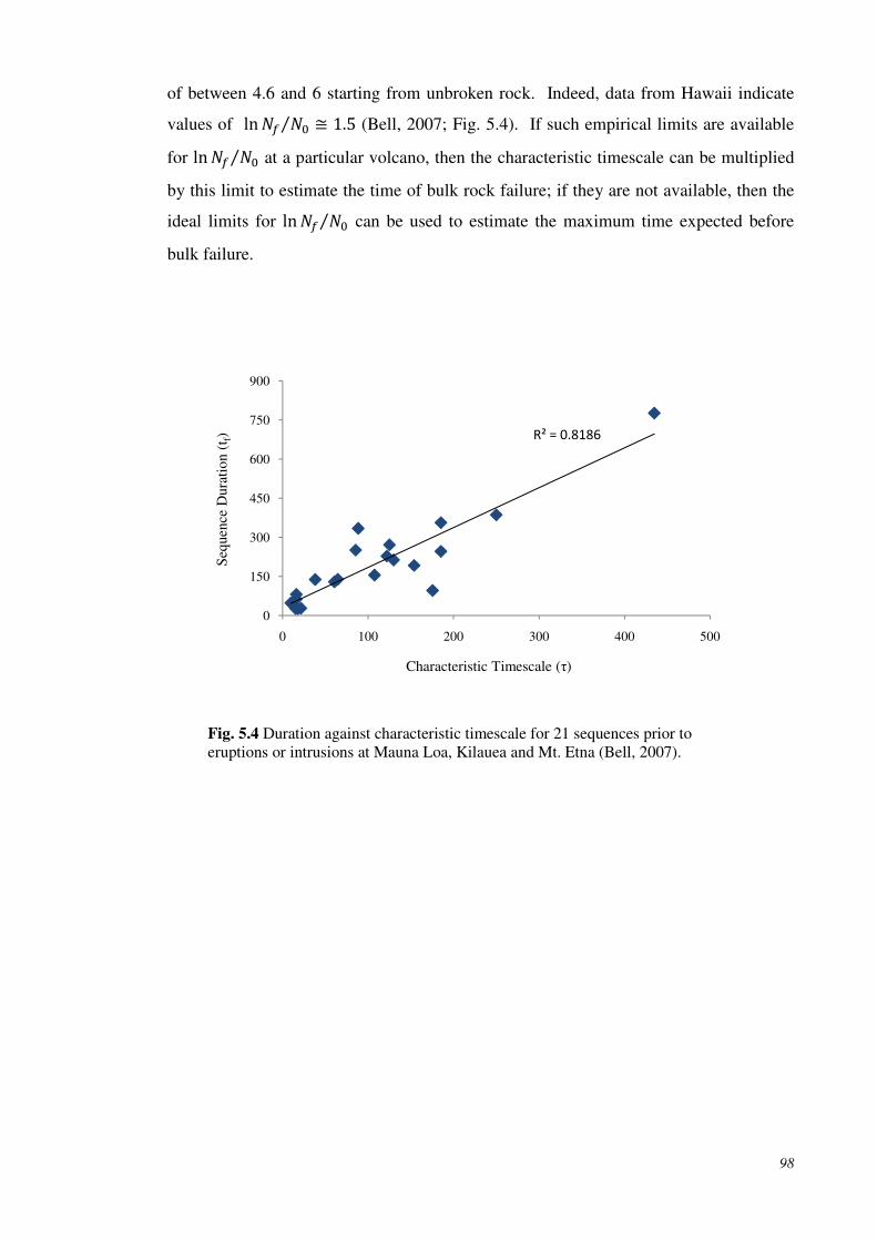
98
of between 4.6 and 6 starting from unbroken rock. Indeed, data from Hawaii indicate
values of ln E " 1.5⁄ (Bell, 2007; Fig. 5.4). If such empirical limits are available
for ln E "⁄ at a particular volcano, then the characteristic timescale can be multiplied
by this limit to estimate the time of bulk rock failure; if they are not available, then the
ideal limits for ln E "⁄ can be used to estimate the maximum time expected before
bulk failure.
Fig. 5.4 Duration against characteristic timescale for 21 sequences prior to eruptions or intrusions at Mauna Loa, Kilauea and Mt. Etna (Bell, 2007).
R² = 0.8186
0
150
300
450
600
750
900
0 100 200 300 400 500
Sequ
ence
Dur
atio
n (t
f)
Characteristic Timescale (τ)

99
5.3 Crack growth properties
Analysis of the characteristic timescales and rate parameters of precursory trends is
important for identifying not only the time to bulk failure, or eruption, but also in
attempting to establish any critical criteria for the transition of an exponential sequence
to hyperbolic growth. Analysis of field and laboratory data is broadly restricted to
evaluating these parameters. However, using the one dimensional numerical model it
is possible to look in more depth at the physical processes causing the observed
characteristic parameters, and the conditions for exponential or hyperbolic growth of
seismic activity. In the field, features such as crack length distributions or the number
of active cracks will be affected by an area much greater than that eventually forming
the open conduit, and even if such parameters were measurable the existence of
surrounding faults and fractures in an edifice would create very noisy data. By looking
at these features in a one-dimensional array it may be possible to understand the cause
of the observed trends; such understanding, in turn, may give some ideas of the
controlling mechanisms that operate in a larger, more realistic setting. This section
looks at a variety of crack growth properties, comparing observations from typical
model outputs for precursory trends of both types I and II, for representative examples
of each type of trend.
5.3.1 Active cracks
Detected seismicity is determined by the activation and growth of faults. Here,
activation refers to when conditions around a fault first become favourable to allowing
that fault to move, and growth refers to repeated movements along the same fault. At a
molecular scale, the mechanism of creating a completely new discontinuity also
becomes important, but such a process cannot be detected directly in the field.
As discussed in Section 3.2.2, the activation of new faults is expected to favour
an exponential increase in event rate with time, whereas the growth and coalescence of
faults is expected to yield a hyperbolic trend. Although the association is empirical, it is
consistent with observations in the field (McGuire & Kilburn, 1997; Kilburn & Voight,
1998; Kilburn, 2003) and laboratory (Lockner et al., 1991; Main & Meredith, 1991).
Thus the approach to bulk failure is expected to be dominated first by fault activation
(yielding an exponential trend with time) and then by fault growth and coalescence
(yielding a faster-than-exponential trend). Increasing beyond a critical number of faults

100
per unit volume is one possible condition that determines the change from activation-
dominant to growth-dominant conditions (Kilburn & Sammonds, 2006). Such a
possibility is investigated here by analysing the distribution of cracks at different stages
within the model simulations.
In each simulation, the first cracks to become activated will be those in regions
of lower general toughness. Additional cracks then become activated as either the
applied stress increases, or local stress intensity increases due to growth of existing
cracks. Two classes of new crack can be identified: (1) a newly activated crack, which
appears as a failed cell, or collection of adjacent cells, that is isolated from any existing
failed cells, and (2) a crack that occurs in a cell close to an existing crack and which can
be related to crack growth.
Figures 5.5 and 5.6 show the number of newly-activated cracks as the model
progresses for Type I and Type II precursory trends, model run 1 and run 2 respectively.
In both cases, the rate of activation increases exponentially, before a significant drop
occurs immediately before failure. The drop is favoured by the coalescence of cracks
and, also, by the model constraint that as more of the cells in the array fail, so the
opportunity decreases for new, isolated cracks to appear. At the present stage of
development, it is not possible to distinguish the primary cause for the final drop-off in
the 1D model. However, such a distinction might be possible in the future by
implementing a two- or three-dimensional array, or incorporating a buffer zone into the
one-dimensional model.

101
Fig. 5.5 Number of newly activated cracks per time step for model run 1 (a) and run 2 (b), Type I and Type II precursory trends respectively. The dashed lines show the best-fit exponential trends prior to the observed drop-off, and the arrow indicates the point at which the Type II trend becomes hyperbolic.
0
15
30
45
60
75
90
0 5 10 15 20 25 30
New
Cra
cks
Time
0
30
60
90
120
0 5 10 15 20 25
New
Cra
cks
Time
a)
b)

102
Fig. 5.6 Log plot of the number of newly activated cracks, before the pre-failure drop-off. Both Type I (red and black squares) and Type II (blue and grey diamonds) precursors show mean exponential activation rates, although each type may show second-order fluctuations about the mean (red squares and grey diamonds). The rate constants for both types cover a similar range of values (0.31 and 0.18 for blue and grey diamonds; 0.29 and 0.22 for black and red squares). The red squares and blue diamonds correspond to model runs 1 and 2 respectively, shown in Fig 5.5. The second Type I (black squares) and Type II (grey diamonds) trends were produced from model runs 3 and 4 respectively.
0
1
2
3
4
5
6
0 5 10 15 20 25 30
ln (
Num
ber
of C
rack
s)
Time

103
Fig. 5.7 (a) Number of active existing cracks (blue diamonds) and the resulting total number of cracks (red squares) with time, for a Type I trend (model run 1). An active existing crack is one that grows during a time step, but has also been active during the previous time step. The total number of cracks includes those that are present in the array but have not yet grown. (b) The proportion of the total number of cracks that grow during a time step.
While new cracks are being activated, existing cracks are also continuing to
grow. The relative effect of crack growth can be inferred from Fig. 5.7 (a) and 5.9 for
Type I precursors, and Figs 5.8 (a) and 5.9 for Type II precursors. The figures show the
variation in the total number of cracks, w, present while the activation rate is
increasing. In all four examples, the total number of cracks maintains a similar value
during the first 50-65% of the increase in activation rate. At the start of a sequence, the
approximately constant total value reflects the small proportion of new cracks being
0
15
30
45
60
75
90
0 5 10 15 20 25 30
Num
ber
of C
rack
s
Time
0
0.25
0.5
0.75
1
0 5 10 15 20 25 30
Prop
ortio
n of
Cra
cks
Act
ivat
ed
Time
b)
a)

104
formed. At longer times, however, the number of newly activated cracks becomes a
significant proportion of the total number; at this stage the total number may increase
(Fig. 5.7a) or begin to decrease (Fig. 5.8a). In the latter case, the increase in number of
activated cracks is being offset by a decrease in total number due to the coalescence of
existing cracks. Eventually, the effect of coalescence dominates until, just before bulk
failure, the experimental array consists of only a small number of large cracks.
In the Type II examples (Figs 5.8 & 5.9), the transition from exponential to
hyperbolic increases in event rate coincides with the onset of a sustained decrease in the
total number of cracks. As expected, therefore, the hyperbolic sequence is characterised
by the emerging dominance of crack growth and coalescence over crack activation.
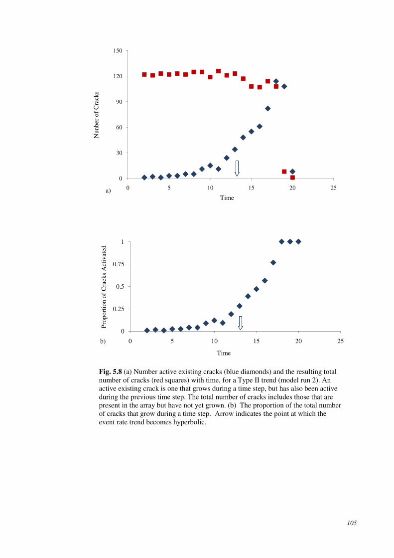
105
Fig. 5.8 (a) Number active existing cracks (blue diamonds) and the resulting total number of cracks (red squares) with time, for a Type II trend (model run 2). An active existing crack is one that grows during a time step, but has also been active during the previous time step. The total number of cracks includes those that are present in the array but have not yet grown. (b) The proportion of the total number of cracks that grow during a time step. Arrow indicates the point at which the event rate trend becomes hyperbolic.
0
30
60
90
120
150
0 5 10 15 20 25
Nun
ber
of C
rack
s
Time
0
0.25
0.5
0.75
1
0 5 10 15 20 25
Prop
ortio
n of
Cra
cks
Act
ivat
ed
Time
b)
a)

106
Fig. 5.9 Total number of cracks for model runs 3 (blue diamonds) and 4 (red squares), Type I and Type II precursory trends respectively. Arrow indicates the point at which the Type II trend becomes hyperbolic.
The change from activation-dominant to growth-dominant conditions may occur
when the number density of cracks exceeds a critical value (Kilburn & Sammonds,
2006). The model results can be used to test this hypothesis because the number density
of cracks is represented by the cumulative number of events. Due to the bounded nature
of the model, the array must progress through the same density changes, resulting in
100% failure, whatever the pattern of event rate produced. The proportion of failed
cells, or density of cracks, in the nine runs for which the exponential-hyperbolic
transition occurred ranges from 4-70%. The single case below 10% corresponds to the
outlier highlighted in Figure 5.3. The remaining, more representative, cases still cover a
range of over 40%. This suggests that the actual density of cracks cannot by itself
determine the mode of acceleration of seismic event rate, or certainly not one that can
be identified from a closed model.
0
30
60
90
120
0 5 10 15 20 25 30
Num
ber
of C
rack
s
Time

107
Fig. 5.10 Proportion of cells that have failed at the point of exponential-hyperbolic transition in nine runs from the Monte Carlo simulation.
5.3.2 Inter-crack distance
In the 1D model, interaction between cracks occurs once the inter-crack distance is on
the order of the crack length. The interaction, in turn, governs the rate at which
neighbouring cracks join up. The mechanism of crack coalescence is therefore
dependent on crack length and inter-crack distance. In understanding the transition to
this mechanism of failure it would be useful to identify any corresponding transitions in
the geometry of cracks. As the model evolves, the distribution of crack lengths will
naturally progress from numerous smaller cracks into, eventually, one large model-
spanning crack at the point of bulk failure. Figure 5.11 shows the progression of mean
crack length in the array for model runs 1 and 2 described in the previous section,
producing Type I and II precursory trends. The model begins with almost entirely
single cell cracks and progresses to a 2,000-cell crack that spans the array at the point of
failure. The mean length in Type I event rate increases almost exponentially during the
middle section of the model run. This precedes a rapid increase in the mean length in
the final stages of the model as failed cells join up to form very large scale cracks (Fig.
5.11). The hyperbolic case appears to follow a similar trend (Fig. 5.11). Figure 5.12
shows the inverse mean crack length for the same two examples. Both inverse trends
tend towards zero, corresponding to an infinitely long crack at the point of failure.
0
1
2
3
4
1 2 3 4 5 6 7
Freq
uenc
y
Density of Cracks
0.1 0.2 0.3 0.4 0.5 0.6 0.7

108
Fig. 5.11 Mean crack length with time, normalised for maximum length (equal to array size) and sequence duration respectively. The two cases show Type I (blue diamonds) and Type II (red squares) precursory trends. Arrow indicates the point at which the event rate trend becomes hyperbolic. Note the logarithmic scale for the vertical axis.
0.0001
0.001
0.01
0.1
1
0 0.2 0.4 0.6 0.8 1
Mea
n L
engt
h/M
axim
um L
engt
h
Time/Sequence Duration

109
Fig. 5.12 Inverse mean crack length with time, for model runs 1 (a) and 2 (b), producing Type I and Type II precursory trends respectively.
Introducing the distribution of inter-crack distance allows for not only the
magnitude but also the geometry of cracks to be considered. The idea of clustering, or
avoidance within a set of cracks is discussed further in Chapter 6. The development of
a fracture network will depend on whether cracks are more likely to grow where
previous cracks exist or in isolation. The mean inter-crack distance decreases very
gradually in the early stage of the model (Fig. 5.13). However, as the cracks grow in
length and occupy a greater proportion of the array, the relative change in the mean with
each incremental decrease in inter-crack distance will become greater.
0
0.25
0.5
0.75
1
0 5 10 15 20 25 30
(Mea
n C
rack
Len
gth)
-1
Time
0
0.25
0.5
0.75
1
0 5 10 15 20 25
(Mea
n C
rack
Len
gth)
-1
Time
a)
b)

110
Fig. 5.13 Mean inter-crack distance with time, normalised for initial mean inter-crack distance and duration of sequence respectively. The two examples show a Type I (blue diamonds) and Type II (red squares) precursory trend. Arrow indicates the point at which the Type II trend becomes hyperbolic.
Both the Type I and II event-rate trends show a similar variation in mean inter-
crack distance with time (Fig. 5.13). After a gradual decrease to about 75% of the
starting mean distance after about 70% of the total duration, the rate of decrease
becomes faster until a crack extends across the whole array (zero inter-crack distance) at
bulk failure. The rate of decrease in the inter-crack distance is not affected by whether
the event rate increases exponentially or hyperbolically, suggesting that the locality of
fracturing is not dependent on the rate of fracturing. However, the initial mean value
for the inter-crack distance in model run 1 was twice that for model run 2. The fact that
initial cracks in the array for the Type II run have a shorter distance between them may
lead to interaction between cracks occurring earlier in the model than in the Type I
example. If this interaction is a mechanism that leads to hyperbolic growth in event
rate, this would suggest that model size may be a limiting factor on the appearance of a
hyperbolic trend, and that in many cases the model has reached bulk failure before the
transition is made. However, the analysis of a greater number of both types of trend is
necessary to investigate this idea further.
0
0.2
0.4
0.6
0.8
1
1.2
0 0.2 0.4 0.6 0.8 1 1.2
Mea
n D
ista
nce/
Initi
al D
ista
nce
Time/Sequence Duration

111
Fig. 5.14 Cumulative distribution function for the inter-crack distance at the (a) outset of the model run and (b) approximately three quarters through the total run time of the model for Type I (blue diamonds) Type II event-rate trends (red squares).
From Figure 5.14a it can be seen that initially the Type I and II examples have
maximum inter-crack distances of a similar scale and that the smaller mean distance, in
the Type II example, is a result of a higher proportion of cracks located close to each
other. While for the Type I case only about 50% of cracks are located within 20 cells of
a neighbouring crack, in the Type II instance this rises to almost 75%. This further
supports the theory that interaction between neighbouring cracks may be the trigger for
hyperbolic growth of event rate. The second plot of cumulative distribution function
corresponds to the time instant 75% of the way through the total run time for each
0
0.25
0.5
0.75
1
0 20 40 60 80 100 120 140
P (
D≤
d )
Inter-crack Distance (d)
0
0.25
0.5
0.75
1
0 20 40 60 80 100 120 140
P (
D≤
d)
Inter-crack Distance (d)
a)
b)

112
model respectively (5.14b). By this stage both cases have a similar proportion of
cracks within 20 cells of a neighbour.
Figure 5.15 illustrates one of the model runs that produced an event rate moving
from exponential to hyperbolic prior to failure, model run five. Initially, the array breaks
along isolated cells. As cracking proceeds, the originally isolated cracks grow and
merge into two principal cracks that extend towards each other. The associated event
rate changes from exponential to hyperbolic when the regions of influence ahead of
each crack begin to overlap (Fig. 5.15). The process is highlighted when only changes
in the number of newly failed cells at each time step are considered (Fig. 5.16). In this
case, activity is clearly confined to an area surrounding the advancing main cracks.

Fig. 5.15 Snapshots of the array II trend (model run 5). hyperbolic trend emerged at t = 15.
The range of the active areas ahead of the crack tips appears to
exponentially from t ~ 10
emerged at t = 15. This emergence of an exponential increase in the active area would
explain the exponential event
trend may be caused by a change in the density of failures within the active region.
However, from Figure 5.18
of cracks within the regions of activity.
the upper and lower
Snapshots of the array at progressive time steps, from a model producing a TII trend (model run 5). Cells that have failed are coloured red, intact cells are blackhyperbolic trend emerged at t = 15.
The range of the active areas ahead of the crack tips appears to
from t ~ 10-12 to failure at t = 18 (Fig. 5.17).
emerged at t = 15. This emergence of an exponential increase in the active area would
explain the exponential event-rate trend, and the switch to a faster than expo
trend may be caused by a change in the density of failures within the active region.
However, from Figure 5.18 it is difficult to define any consistent increase in the density
of cracks within the regions of activity. A slight jump in the density
sections at the emergence of the hyperbolic event rate. However,
113
teps, from a model producing a Type Cells that have failed are coloured red, intact cells are black. The
The range of the active areas ahead of the crack tips appears to grow
The hyperbolic trend
emerged at t = 15. This emergence of an exponential increase in the active area would
rate trend, and the switch to a faster than exponential
trend may be caused by a change in the density of failures within the active region.
it is difficult to define any consistent increase in the density
jump in the density is seen in the both
ce of the hyperbolic event rate. However,

this is only temporary and in fact the density fluctuates around a mean value for much
of the run time of the model.
Fig. 5.16 New failures at progressive time steps in model run failed during the previous time step are coloured yellow
Cell = 1
500
1000
T = 12
this is only temporary and in fact the density fluctuates around a mean value for much
of the run time of the model.
es at progressive time steps in model run 5 (Fig. 5.1failed during the previous time step are coloured yellow.
T = 12 T = 13 T = 14 T = 15 T = 16 T = 17
114
this is only temporary and in fact the density fluctuates around a mean value for much
ig. 5.15). Cells that have
T = 18
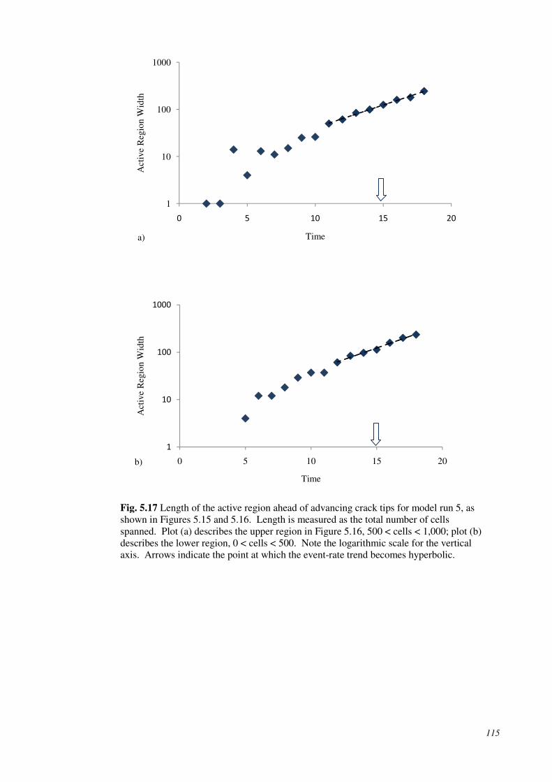
115
Fig. 5.17 Length of the active region ahead of advancing crack tips for model run 5, as shown in Figures 5.15 and 5.16. Length is measured as the total number of cells spanned. Plot (a) describes the upper region in Figure 5.16, 500 < cells < 1,000; plot (b) describes the lower region, 0 < cells < 500. Note the logarithmic scale for the vertical axis. Arrows indicate the point at which the event-rate trend becomes hyperbolic.
1
10
100
1000
0 5 10 15 20
Act
ive
Reg
ion
Wid
th
Time
1
10
100
1000
0 5 10 15 20
Act
ive
Reg
ion
Wid
th
Time
a)
b)

116
Fig. 5.18 Density of failed cells in the regions of activity ahead of advancing cracks for model run 5, as described in Figures 5.15 – 5.17. Plot (a) describes the upper region in Figure 5.16, 500 < cells < 1,000; plot (b) describes the lower region 0 < cells < 500.
0
0.2
0.4
0.6
0.8
1
0 5 10 15 20
Den
sity
of
Fai
led
Cel
ls
Time
0
0.2
0.4
0.6
0.8
1
0 5 10 15 20
Den
sity
of
Fai
led
Cel
ls
Time
a)
b)

117
5.4 Stress distribution
As the dominant failure mechanism changes from fault activation to fault growth, the
relative influence of the remote and local stresses may change in the model. Initially
failure is driven by the level of remotely applied stress and cells throughout the array
would be equally likely to fail, dependent only their assigned fracture toughness. As the
mechanism becomes dominated by crack growth, the concentration of stress around the
larger cracks would exert a greater influence on the stress field and favour failure in
already highly fractured areas. This assumption can be tested by looking at the
distribution of stress intensity across the array as the model progresses. As described in
Chapter 4, the stress intensity increases in cells around the tip of a crack depending on
its length and the proximity of neighbouring cracks. The density distribution of stress
intensity magnitude across the array is therefore an alternative measure of the variable
geometry of cracks.
Figure 5.19 shows how the cumulative distribution function of stress intensity
magnitude varies as the model evolves. For cells located outside the range of influence
of failed cells, the stress intensity is just the remotely applied stress. Initially, there are
relatively few cracks in the array and therefore this applies to the majority of cells (Fig.
5.19a). Initially, in both the Type I and Type II examples, over 80% of cells have this
minimum magnitude of stress intensity, equal to the remotely applied stress. This
minimum point is highlighted for each example in Figure 5.19 by a dashed line. As the
model evolves and more cracks appear along the array, a greater number of cells will be
within the range of influence of these cracks. This will cause the range of stress
intensity magnitudes across the intact cells to increase. At two thirds through the
duration of the model run, the isolated cells still account for the greatest proportion of
stress intensity frequencies (Fig. 5.19b), and there are a high percentage of cells that
remain isolated right up until the final stages of failure. This effect is more pronounced
in the Type I event-rate case. The Type II example shows a faster decrease in the
proportion of cells that are not affected by any neighbouring cracks. In other words,
cells fall into the range of influence of cracks more quickly in this second case. This
would be expected if the failure mechanism was dominated by the interaction and
coalescence of exiting cracks, over the activation of new, isolated cracks.

118
Fig. 5.19 Cumulative distribution function F for stress intensity factor, normalised for maximum stress intensity, over all cells at (a) the start of the model run and (b) approximately two thirds through the total run time of the model. F(K/Kmax) describes the probability that the normalised stress intensity is less than or equal to the specified ratio. The two examples shown are for model run 1 (blue diamonds) and model run 2 (red squares), producing Type I and Type II event-rate trends respectively. Plot (b) shows F at the point at which the Type II trend becomes hyperbolic. The dashed lines show the value of the remotely applied stress, normalised for maximum stress intensity, and therefore represent the minimum stress intensity for each example. Note the logarithmic scale for the horizontal axis in plot (b).
0.5
0.6
0.7
0.8
0.9
1
0 0.2 0.4 0.6 0.8 1 1.2
F(K
/Km
ax)
K/Kmax
0.5
0.6
0.7
0.8
0.9
1
0.001 0.01 0.1 1
Fk
(K/K
max
)
K/Kmax
b)
a)

119
5.4.1 Proximity to failure
The failure of cells in the array is controlled not only by stress intensity but also by the
distribution of fracture toughness. The ratio of stress intensity to fracture toughness
gives a measure of a cell's proximity to failure, with the limiting values of 0 and 1
corresponding to the conditions of no potential for failure and of imminent failure.
Changes in the overall distribution of proximity to failure can highlight differences in
the mechanism of failure Figure 5.20 shows the distribution function for this
measure of proximity to failure at different stages throughout the run time of the
example models 1 and 2. Figure 5.19a showed a near constant distribution of stress
intensity at the start of the model runs. Due to the randomness of the fracture toughness
across the array’s cells, the initial distribution function shows more variety than the
approximate step function that would otherwise be expected (Fig. 5.20a). However,
with over 60% of intact cells having a ratio value between 0.3 and 0.5, there is still
some regularity in the likelihood of failure across the array in both examples. As the
model evolves there is a tendency to a more linear trend in the distribution function,
highlighting a much greater difference in the proximity to failure across the remaining
intact cells. The linearity is especially pronounced in the Type II example, with a fit of
0.99 for the range of K/Toughness from 0.4 to 0.8. For the Type I example, the
range from 0.7 – 1 also provides a linear fit with 0.99.

120
0
0.2
0.4
0.6
0.8
1
0 0.2 0.4 0.6 0.8 1 1.2
F (K
/Tou
ghne
ss)
K/Toughness
0
0.2
0.4
0.6
0.8
1
0 0.2 0.4 0.6 0.8 1 1.2
F (K
/Tou
ghne
ss)
K/Toughness
a)
b)

121
Fig. 5.20 Cumulative distribution function for the ratio of stress intensity to fracture toughness over all intact cells of the one-dimensional array for model runs 1 (blue diamonds) and two (red squares), producing Type I and Type II event-rate trends respectively. The distribution function is shown at: (a) the start of the run, (b) approximately two thirds through the total run time of the model, and (c) approximately 85% through the total run time of the model. Dashed lines show the range of linearity of the cumulative distribution function for each example. Plot (b) shows the point at which the Type II example switches to a hyperbolic event rate.
Failure dominated by the appearance of new cracks or newly activated cracks
corresponds to randomness in the probability of failure across a domain. Any cell is
just as likely as another to fail, and this corresponds to a random uniform proximity to
failure for all cells across the array. However, once the mechanism of failure has
switched to the extension and coalescence of existing cracks, this leads to a much
greater variety in the proximity to failure across the array’s intact cells. Regions
surrounding extending cracks will be a lot more likely to fail than isolated cells, as the
stress intensity in the former will be increased by the presence of neighbouring cracks.
As these cracks grow larger, it becomes more and more likely that the intensity will
exceed a cell’s fracture toughness. Isolated cells maintain the same stress intensity until
they eventually fall into the range of influence of an approaching crack. The change
over the course of the model runs, from an initial, more uniform, proximity to failure to
a final, almost linear, distribution function is therefore consistent with the theory of a
change in failure mechanism from the appearance or activation of new isolated cracks to
the extension of existing cracks.
0
0.2
0.4
0.6
0.8
1
0 0.2 0.4 0.6 0.8 1 1.2
F (K
/Tou
ghne
ss)
K/Toughness
c)

122
5.5 Alternative precursory trends
The Monte Carlo simulation of the one-dimensional model captures the common
behaviour of exponential and hyperbolic event-rate trends in the field. The simulations
also produce alternative, less frequent trends, in which the faster than exponential
sequence appears as a step like increase (Fig. 5.21). In the model this style of activity
appears to correspond to a relatively homogeneous distribution of fracture toughness.
At one extreme, with a low value of both the mean and variance of fracture toughness, a
large number of cells fail almost instantly when stress is applied to the array (shown by
the red squares in Figure 5.21). Remaining intact cells then tend to fail in quick
succession due to the large number of surrounding cracks. At the other extreme, where
fracture toughness again has a small variance but now with a much larger mean value,
the model progresses with very few failing cells at each time step, creating a low
background level of activity, and only once the applied stress has reached a critical
point does the same effect occur of multiple cells, with similar fracture toughness
values, failing simultaneously (blue diamonds in Figure 5.21). Although within the
Monte Carlo simulation these two cases are seen as opposite extreme cases, they are in
fact recording the same process. Whether stress has built up gradually or there is a
rapid step like increase, the outcome of a large number of cells suddenly failing is the
same.
Fig. 5.21 Event rate plots from two model runs showing faster than exponential, step like increases in rate prior to failure.
0
100
200
300
400
0 20 40 60 80 100 120 140
Num
ber
of e
vent
s
Time

123
An interesting future direction for this research would be to investigate the
occurrence of these step-like increases in precursory activity in the field. A sharp
increase in seismic energy and earthquake event rate was observed prior to the 1956
eruption of Bezymianny, Kamchatka (Tokarev, 1985), (Fig. 5.22). This explosive
eruption followed 1,000 years quiescence, with a noticeable increase in seismic activity
beginning approximately a month before the eruption. However, no further analysis on
the nature of this trend was provided by the author, and it should be noted that activity
leading up to the eruption may have been missed through lack of monitoring. A very
sharp increase in earthquake numbers was also seen in the days prior to explosive dome
eruptions in 1959 and 1960. Similar rapid increases in event rate were recorded prior to
the 1964 eruption at Sheveluch, which ended 15 years of quiescence, and again prior to
a later paroxysmal dome explosion in 1993 (Tokarev, 1985). In both cases seismic
unrest was noted several weeks prior to eruption.
Fig. 5.22 The intensity of earthquakes per day prior to eruption (tu) at Shiveluch, 1964 (1), Bezymianny, 1956 (2), and Mt. St. Helens, 1980 (3) (Tokarev, 1985). Intensity is measured as the average number of daily earthquakes.
The appearance of faster than exponential, step-like trends in the literature suggests that
the one-dimensional model may also be utilised to anticipate alternative precursors in
the future. In addition, occurrences in the field of a step increase in seismicity may be
caused by a similar process to the model, implying the presence of a relatively
homogeneous edifice.

124
5.6 Chapter summary
Exponential trends are commonly produced by the one-dimensional model, similarly to
observations in the field and laboratory. In all three situations, examples of the
emergence of a faster-than-exponential trend are also observed. Properties of crack
growth in the model support the theory of a switch in dominating failure mechanism
producing the two different trends. The exponential sequence is associated with the
activation of new cracks. Once growth and coalescence of existing cracks becomes the
favoured failure mechanism, the hyperbolic trend emerges. A second faster-than-
exponential precursor is produced by the model, in the form of a step increase in
seismicity. This type of activity has also been recorded prior to eruptions.
The exponential sequences produce a characteristic timescale for the precursory
activity. This timescale can be related to the expected duration of the sequence, and
therefore with the time to failure and eruption.
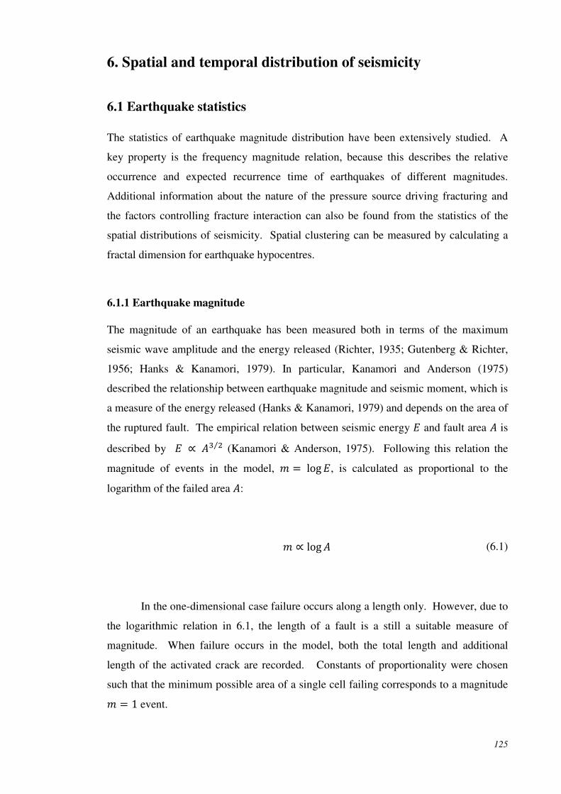
125
6. Spatial and temporal distribution of seismicity
6.1 Earthquake statistics
The statistics of earthquake magnitude distribution have been extensively studied. A
key property is the frequency magnitude relation, because this describes the relative
occurrence and expected recurrence time of earthquakes of different magnitudes.
Additional information about the nature of the pressure source driving fracturing and
the factors controlling fracture interaction can also be found from the statistics of the
spatial distributions of seismicity. Spatial clustering can be measured by calculating a
fractal dimension for earthquake hypocentres.
6.1.1 Earthquake magnitude
The magnitude of an earthquake has been measured both in terms of the maximum
seismic wave amplitude and the energy released (Richter, 1935; Gutenberg & Richter,
1956; Hanks & Kanamori, 1979). In particular, Kanamori and Anderson (1975)
described the relationship between earthquake magnitude and seismic moment, which is
a measure of the energy released (Hanks & Kanamori, 1979) and depends on the area of
the ruptured fault. The empirical relation between seismic energy # and fault area is
described by # S ⁄ (Kanamori & Anderson, 1975). Following this relation the
magnitude of events in the model, log #, is calculated as proportional to the
logarithm of the failed area :
S log (6.1)
In the one-dimensional case failure occurs along a length only. However, due to
the logarithmic relation in 6.1, the length of a fault is a still a suitable measure of
magnitude. When failure occurs in the model, both the total length and additional
length of the activated crack are recorded. Constants of proportionality were chosen
such that the minimum possible area of a single cell failing corresponds to a magnitude
1 event.

126
6.1.2 Magnitude distribution: The Gutenberg-Richter Law
The frequency magnitude distribution for earthquakes has proven to be one of the most
important statistics in the analysis of seismic activity. The distribution, which was first
described by Ishimoto and Iida in Japan (Ishimoto and Iida, 1939) and then by
Gutenberg and Richter in California (Gutenberg & Richter, 1944), is described by the
relation:
log * u (6.2)
where is the number of earthquakes with magnitude greater than or equal to . The
gradient u is known as the seismic b-value. This power law relation between the size
and frequency of seismic events has become known as the Gutenberg-Richter Law.
Figure 6.1 shows magnitudes and frequencies for earthquakes worldwide during 2007
(USGS, 2007). The cumulative number of earthquakes can also be written in terms
of seismic energy #, as S #<. The exponent is a function of the seismic b-value.
Fig. 6.1 Frequencies of global earthquakes in 2007 (www.usgs.com). N is the number of events with a magnitude greater than m. The linear log relationship for 5 is that described by the Gutenberg-Richter Law. Below 5 the catalogue of earthquakes is incomplete as the magnitudes become too low for observation.
0
1
2
3
4
5
0 2 4 6 8 10
Log
(N)
Magnitude (m)

127
Fig. 6.2 Typical frequency-magnitude distribution for the one-dimensional model. N is the number of events with a magnitude greater than m. Lower magnitudes provide a good fit to the Gutenberg-Richter Law, with a deviation from a linear fit for 1.7.
The expression (6.2) describes a self-similar relationship and has been shown to
describe both global and regional earthquake catalogues, as well as acoustic emissions
produced by compressional rock fracture experiments in the laboratory (Scholz, 1968).
Further supporting the universality of this relationship, the seismic b-value, shown as
the linear slope of the logarithmic graph (Fig. 6.1) is typically found to be close to one
at all scales of observation.
As with other examples of self-similarity in nature, limits of dimension prevent
true scale invariance. In the case of earthquake magnitude, a finite limit to fault size
provides an upper limit to possible earthquake magnitudes. Gutenberg and Richter
(1949) observed a lack of events of magnitude 8 and greater. A deviation from large
amplitude events in the laboratory has also been recorded (Scholz, 1968), as sample
dimensions provide a limit to potential fracture size. A drop-off in the frequency-
magnitude relation observed in volcanic settings (Qamar et al., 1983) has been
attributed to inhomogeneous stress conditions. Observation becomes a problem at the
lower scale range with events becoming too small for monitoring equipment to detect.
There is therefore often a drop off away from the linear trend toward smaller magnitude
values, which can be observed in the earthquake catalogue in Figure 6.1. The lower
limit to the power law relation is defined as the magnitude of completeness <.
Figure 6.2 is a typical output from the one-dimensional model, run under
constant stress, where magnitudes are recorded by the number of simultaneously failing
0
1
2
3
4
0.5 1.5 2.5L
og(N
)
Magnitude (m)

128
adjacent cells. The frequency-magnitude distribution provides a good fit to the
Gutenberg-Richter Law, particularly at lower magnitudes. The fall-off from the linear
trend at higher magnitudes implies a lack of large scale events. Similarly to the
dimension limits in the laboratory, the number of cells in the model provides a
theoretical upper limit to the possible event size. Previously failed cells distributed
throughout the model restrict the potential length of adjacent simultaneous failures,
leading to a much lower limit in practice.
The seismic b-value is inversely proportional to the mean magnitude. Therefore
any variation in space or time of the b-value is also highlighting a variation in the mean
magnitude. The measurement of magnitude can vary from location to location
depending on coverage, instrumentation and analysis techniques. The seismic b-value
therefore provides a more objective method of comparing magnitude distributions.
6.1.3 Seismic b-value
The Gutenberg-Richter Law is assumed to hold over all magnitudes where data
are complete. However, it has been observed that the frequency-magnitude distribution
can deviate from this linearity within the completeness range (Urbancic et al., 1992;
Rydelek & Sacks, 1989; Taylor et al., 1990). This has been particularly noted in
volcanic regions (Main, 1987). Earthquake swarms produced by magma movement
may increase the number of small events or more importantly events of a similar
magnitude and therefore create a bimodal frequency-magnitude distribution (Wiemer &
Wyss, 2002). The b-value is a measure of the relative numbers of large and small
magnitude events. A larger value describes a relative increase in the number of small
events, and a smaller value a relative increase in the number of large events. Although
b is generally found to lie close to one in the crust, it has often been observed closer to
two and three, beneath volcanoes (Power et al., 1998; Wyss et al., 2001; Wiemer &
McNutt, 1997). High b-values have been attributed to increased material heterogeneity
(Mogi, 1962), increased local stress (Scholz, 1968; Huang & Turcotte, 1988), high pore
pressure (Wyss, 1973), and large temperature gradients (Warren & Latham, 1970).
All of these properties can be associated with the presence of magma and high b-
value anomalies at volcanoes have been used to provide constraints on the possible
location of magma reservoirs or intrusions (e.g. Pinatubo, Sanchez et al., 2004;
Makushin, Bridges & Gao, 2006; Etna, Murru et al., 2007). Fracturing around a body

129
of magma will lead to greater heterogeneity of the host rock, while interaction between
magma and groundwater can lead to increased pore pressure (Wiemer & McNutt, 1997).
An increase in pore pressure reduces effective stress, allowing for more slip on existing
fractures, rather than the creation of new fractures (Murru et al., 2007). This creates a
larger proportion of small events, leading to an increase in b-value. Larger events are
more easily sustained in cooler, less fractured rock away from intruded regions (Power
et al., 1998). Hence higher temperatures will favour a relative decrease in the number
of larger events, so also producing an increase in b-value (Sánchez et al., 2004).
Spatial variations
Spatial variations in the seismic b-value have been studied at numerous volcanoes
(McNutt, 2005). Studies show a high degree of spatial variation, with areas close to a
normal value of u~1 occurring adjacent to areas with anomalously high values in the
range 1.5 H u H 3. It is therefore now suggested that rather than volcanic regions as a
whole having a high b-value, it may be more the case that pockets of high b-values exist
in crustal rock producing otherwise normal or even low b-values (Wiemer & Wyss,
2002). The high anomaly values tend to occur at depths of less than 7km and are
assumed to relate to the presence of magma bodies (McNutt, 2005). Weimer and Wyss
(2002) suggest that a high b-value anomaly is a necessary but not sufficient condition
for the presence of magma. Difficulties in building a clear representation of a spatial
variation in b beneath a volcano are due to the high number of low magnitude events.
Fewer are recorded, and therefore a large area or volume must be sampled in order to
contain a large enough number of events to be statistically significant. Resolution may
become too low, and any variation lost (Wiemer & Wyss, 2002).
At Montserrat a high b-value anomaly was found in the region about 2 km
below the active crater area. During the period over which the study was conducted,
increased fumarolic activity and ground cracks were observed in this region, suggesting
again that increased heterogeneity or temperature may have caused the increase (Power
et al., 1998). Two regions of high b-value at Pinatubo were situated next to the inferred
location of a magma body derived from P-wave velocity analysis (Sánchez et al., 2004).
A high b-value anomaly beneath Mt. St. Helens was again found to correlate
with an inferred shallow magma reservoir (Wiemer & McNutt, 1997). Areas of high b-
value also coincided with regions of an increase in total number of events, and a

130
maximum magnitude approximately one unit smaller than surrounding areas with
normal b-values.
The South flank of Kilauea is slipping seaward on a decollement plane. High b-
values beneath the flank are recorded at a depth of approximately 6 km, decreasing to
anomalously low values of u 0.4 at depths greater than 8 km depth (Wyss et al.,
2001). The high values are again associated with the presence of a magma body beneath
the East Rift zone, whereas the low value at greater depth is thought to be an indication
of the relatively homogeneous nature of the decollement plane and the potential for
larger slips or ruptures (Wyss et al., 2001).
Temporal variations
Studying a temporal change in b in the field is inherently more difficult as consistent
data sets are often not available. Any change in instrumentation or analysis procedures
may influence the magnitude distribution and hence the b-value (Zuniga and Wyss,
1995). Hypocentre migration with time also makes temporal variation analysis difficult.
A temporal shift can also coincide with a spatial shift, making it difficult to ascertain
whether b is varying with time, space or both (Murru et al., 2007; McNutt, 2005).
A significant increase, followed by a sharp decrease in b is reported prior to two
eruptions at Mt. Etna (Gresta & Patanè, 1983a; 1983b). An increase followed by a drop
in b-value has also been observed leading up to large earthquakes (Smith, 1981). Under
the stress regime hypothesis, this decrease would correspond to an increase in local
stress leading up to an eruption. A sharp peak followed by a dip in b-value was
observed before a phreatic eruption preceding the 18th May explosive eruption at Mt. St.
Helens in 1980 (Main, 1987). However, no definitive precursory trend was noted
leading up to the main 18th May eruption (Qamar, 1983). Similarly, no significant
temporal change in b was found before or after the 1991 Pinatubo eruption (Sanchez et
al., 2004).
As a precursory tool a similar problem exists as with measuring spatial variation
in b. The resolution of time interval that must be sampled in order to include sufficient
events for a statistically significant measurement may conceal any short-term variation
in the b-value (Main, 1987).
Laboratory tests

131
Acoustic emissions produced during tensile fracture tests in the laboratory have
amplitude correlated with crack length growth in a similar relation to earthquake source
and magnitude (Lockner, 1993). Acoustic emissions during compression tests are
linked to the propagation and interaction of microcrack arrays. Scholz (1968)
demonstrated that microfracture events during rock deformation experiments also
follow the Gutenberg-Richter Law and that b decreased as stress was increased. This
relationship can be described by a statistical model of fracture growth (Scholz, 1968).
A decrease in b is often observed before failure in both tension and compression tests in
laboratory rock fracture experiments. It has been shown that the b-value is linearly
related to stress intensity factor 3:
u R * 3 (6.3)
where R and are constants (Meredith & Atkinson, 1983). Meredith et al. (1990) used
relation (6.3) to explain and predict the decreases in b-value recorded prior to failure,
which have been linked to an increase in stress intensity (Main et al., 1992; Sammonds
et al., 1992). Stress intensity increases with fracture length, and therefore decreases in
b-value arise when fractures lengthen and unite. This occurs just before bulk failure.
Compression tests carried out at temperatures up to 900°c and 50MPa confining
pressure found a minimum in b coincident with macroscopic failure (Smith, 2006).

132
6.1.4 Evolution of seismic b-value in the 1D model
Calculation of b-value
Given that the seismic b-value is such a widely analysed earthquake statistic, the
methods used to estimate b are also important to consider. A simple least squares
method can be used to calculate the slope of the linear relation (6.2). However, this
method assumes a Gaussian distribution for residuals that leads to a disproportionate
influence on the result by the few larger magnitude events (Page, 1968). Many studies
therefore use a maximum likelihood estimate of b, as derived by Page (1968):
u log I F * '4 * 'XI6''U71 * I6''U7 G
(6.4)
where u ln 10, is the mean magnitude and '4 and 'X are the minimum
and maximum magnitudes respectively. Equation (6.4) can be solved numerically for u.
Alternatively, if the magnitude range is sufficiently large, for example 'X * '4 2 (Page, 1968), it can be approximated by (Aki, 1965):
u log I * '4 (6.5)
Due to the logarithmic form of the length to magnitude relation and the scale of the one-
dimensional model, the model data will not cover a sufficiently large range of
magnitudes. The minimum magnitude event, corresponding to the failure of a single
cell, is 1. Occurrence of a 3 event requires the simultaneous failure of 100
adjacent cells. Damage zones around extending cracks and the distribution of
microcracks throughout the model make this scale of event very improbable, as there is
unlikely to be a fully intact section of this length. The lack of larger events results in a
considerably high b-value. However, a comparison of values and overall trends can still
provide a useful analysis, without concern of the absolute figures. It should also be
noted that large magnitude events are in any case rarely observed in volcanic regions,

133
and due to factors previously discussed, b-values can be higher than average. In the
model, b-values were calculated originally using a bisection method on Equation (6.4)
to numerically solve for b. When derived to within a tolerance of 0.01 magnitude units,
results were consistent with those produced by the approximation formula (6.5). For
ease of computation, therefore, this approximation was used throughout.
The derivation of the maximum likelihood estimate also assumes a continuous
range of magnitudes. As magnitude values correspond to the number of failed cells in
the model, there is a discrete distribution of values. However, this is similar to the
grouping of earthquake magnitudes in the field and for a group width, or resolution, of
less than 0.1 magnitude units Equation (6.4) remains a good approximation (Bender,
1983). Due to the logarithmic relation in (6.2), magnitude group widths in the model
are not equal, but become smaller with increasing magnitude, which makes the use of
maximum likelihood estimates for grouped data inappropriate (Bender, 1983; Palacios
et al., 2006). Because the group width is a maximum of 0.3, and rapidly falls below 0.1
units, Aki’s continuous formula is used.
The minimum recorded magnitude in the model, '4, is the failure of a single
cell and corresponds to 1. The minimum magnitude used in calculating b should
be the minimum value in the corresponding magnitude group (Palacios et al., 2006).
Using '4 1 in calculating b may lead to considerably larger values, as the
denominator in Equation (6.5) can be of the order of 10-2. As with field data, and in
accordance with the assumption of a continuous range of magnitudes, it is assumed that
1 is the midpoint of a magnitude group, and that '4 H 1. The group width is
taken to be equal to the difference between the first two discrete magnitude values
observed in the model, giving '4 1 * ~0.85. Choice of '4 modifies the
scale of the b-value distribution but has no effect on the overall trend of the variation.

134
A least squares value was also estimated for each b-value calculation. Where no
inconsistency was observed between the two estimators, the maximum likelihood
estimate was the value reported. The standard error of b is calculated using the method
of Shi and Bolt (1982). For a large sample size w, the standard error is given by:
ulog I ∑6 4 * 7
w6w * 17 (6.6)
To produce a statistically significant b-value, the number of events in the
catalogue used must be sufficiently large (e.g. w 100, Wiemer & McNutt, 1997;
Power et al., 1998). Events are selected within a moving window over time or space,
with an overlap of events between successive windows.
Temporal variation
The variation of b-value with time was studied for both constant and increasing stress.
A sliding window of 300-1,000 events was used, progressing by 50 events with each
calculation. Event counts produced by the model provide a discrete rather than
continuous time series, with no meaningful ordering of events within each time step. It
was therefore important to include sufficient events in each calculation to avoid an
arbitrary proportion of events within one time step creating an individual grouping of
events. A minimum window size of 300 events was chosen as a good balance between
exceeding the maximum number of events in one time step and producing enough b-
values for a non-trivial analysis. To further mitigate the effect of a discrete time series,
b-values were also calculated from data sets in which the order of events within each
time step had been randomised. No significant variation in the results was observed.
Using windows of equal time period also eliminated this problem. However, as event
rate typically changes significantly during an individual run of the model, this leads to a
considerable variation in the number of events per calculation. The same time interval
towards the start of the model run will contain much fewer events than an equal time
interval towards the end of the run. Nevertheless, consistency of results under different
sampling techniques provides a useful test (Sanchez et al., 1994), and when this equal
time window method was tested, again little qualitative difference was seen in the
resulting b-value trend.

135
Fig. 6.3 Variation of b-value with time, under increasing stress conditions. A sliding window of 500 events is used for each calculation, advancing 50 events at a time. Vertical bars indicate the standard error.
Figure 6.3 shows a typical b-value trend with time until failure from a model run
under increasing stress. The value tends to decline gradually over the entire time
period, although fluctuations are also observed as seen in Figure 6.4, showing a model
run under constant stress. However, independent of the style of decrease the b-value
reaches a minimum at the point of failure. Both a gradual decrease and a minimum
value at failure are consistent with deformation studies in the laboratory (e.g. Meredith
& Atkinson, 1983; Smith, 2006; Scholz, 1968; Main et al., 1989).
1
2
3
051015
b-v
alue
Time to failure

136
Fig. 6.4 Variation of b-value with time, under constant stress conditions. A sliding window of 500 events is used for each calculation, advancing 50 events at a time. Vertical bars indicate the standard error. Fluctuations occur in the gradual decline of b-value with time.
Fig. 6.5 Variation of b-value with time (blue diamonds) under increasing stress conditions. Red triangles show the average stress intensity over all intact cells, normalised for fracture toughness.
Figure 6.5 shows b-values for the same data set as used in Figure 6.3, but here
each window contains 1,000 events. The triangles represent the average stress intensity
factor over all intact cells in the model, normalised with fracture toughness at each cell.
A gradual decrease can still be seen for the b-value, although some variation has been
lost at this lower resolution. The decreasing b-value corresponds to a steadily
1
1.4
1.8
2.2
024681012
b-v
alue
Time to failure
0
0.2
0.4
0.6
0.8
0
1
2
3
0123456
Mea
n K
/Kc
b-v
alue
Time to failure

137
increasing value of 3 3<⁄ . The later section of the plot shows a quasi-linear relation
between b-value and stress intensity, of the nature described by Main et al. (1989) in
expression (6.3). However, the first three pairs of data points show a similar scale of
decrease in b accompanied by first a large then very minor increase in stress intensity.
This suggests that stress intensity may not be the sole factor affecting b-value variation.
The range of magnitudes produced by the model is small compared with
earthquake catalogues from the field. Larger magnitude events in the model are rare
partly due to the damage that builds up around extending fractures. The distribution of
existing small cracks in these regions prevents a significant number of adjacent cells
failing simultaneously. For example, while a major crack may appear to propagate a
length on the order of 100 cells in a single iteration, producing a 3 event, this will
in fact have been made up of numerous much smaller events linking up failed cells in
the region around the tip of the major crack. However, this may be a similar mechanism
to that which contributes to the b-value in volcanic settings higher than the expected
u~1 for tectonic earthquakes. Highly fractured material is likely at volcanoes due to
the many processes occurring (Sánchez et al., 2004) and therefore in the same fashion,
the host rock is not capable of sustaining a large event but instead produces many
smaller events (Wiemer & McNutt, 1997).
Fig. 6.6 Variation of b-value (blue diamonds) with time under constant stress conditions. 500 events were used for each calculation. The maximum (red squares) and minimum (red triangles) recorded magnitude for each window of events is also shown. Magnitudes are calculated using the total length of active cracks.
0
1
2
3
4
5
0
0.5
1
1.5
2
0246810
Mag
nitu
de
b-v
alue
Time to failure

138
A second measure of magnitude is introduced that records the extension of a
crack by the coalescence of numerous smaller cracks as a single event. A consequence
of this method of measurement is the occurrence of larger magnitude events than were
previously possible, the array dimensions providing the only limit on size. Figure 6.6
shows a typical b-value distribution calculated for this magnitude range, under constant
stress conditions. The existence of larger magnitude events reduces b, but the overall
trend of the distribution remains the same. A gradual decrease is observed, with the
minimum b-value occurring at the time of failure. Whether it is assumed that
magnitude measurements represent the joining together of adjacent fractures, or the
extension of a single, major fracture, the b-value still decreases with time to a minimum
before failure. Figure 6.6 also shows the maximum and minimum magnitudes observed
in each window of events. From Equation (6.4), b is dependent on the mean magnitude
rather than the spread, or range. This is highlighted by the continuing decrease in b-
value, while the magnitude range remains constant.
Fig. 6.7 Variation of b-value (blue diamonds) with time. Re triangles show applied stress, normalised by the maximum applied stress. The model reached equilibrium after the drop in stress with intact cells remaining.
No significant difference is seen in the b-value under constant or increasing
stress. The range of b and the decrease with time are also consistent over different
trends for event rate with time (e.g. Figs. 6.4 & 6.6). The resolution issue of including a
sufficient number of events in each calculation window may mask any variations with
different event rate trends. However the consistency in results implies that while the
number of events may increase at various rates, the distribution of magnitudes of those
0
0.2
0.4
0.6
0.8
1
0
0.5
1
1.5
2
2.5
100 250 400 550 700 850
Nor
mal
ised
str
ess
(σ/σ
max
)
b-v
alue
Mid-window event

139
events does not change. Figure 6.7 shows that a similar trend is also seen when, after a
drop in applied stress, the model does not fail, but reaches equilibrium with cells still
intact. A significant reduction in applied stress appears to have no immediate effect on
b, implying a greater dependence on fracture geometry rather than on background stress.
Once fractures have formed in the model, they do not heal in the event of a stress drop.
If the b-value depends on the size-frequency distribution of fractures then it would be
expected for b to remain the same. The similarity of the trend observed when the model
did not run to failure (Fig. 6.7) with those that did, implies a difficulty in using this as a
method to forecast model behaviour.
While the observations from the model for temporal b-value variation are
consistent with those produced in laboratory experiments and seen in field data, they
suggest a limited useful function as a forecasting tool. Failure is generally coincident
with a minimum in b. However, in real time analysis there would be no way to
distinguish this data point from each previous minimum, without a known critical value
for b (Main et al., 1993).
Spatial variation
For completeness, the spatial variation of the seismic b-value was also calculated. It has
been suggested that regions of high b-value in volcanic regions correspond to the
location of magma bodies. Processes caused by magma intrusions create greater
material heterogeneity than in surrounding regions. In the model, a uniform remote
stress is applied and the fracture mechanism is the same throughout the array.
Figure 6.8a shows the spatial variation of b calculated from windows of 300
events, with an overlap of 250 events, under increasing stress conditions. The location
of an event is taken as the centre of adjacent failing cells. Magnitudes are measured
using the length of new failing cells only. The slight increase in b-value toward the
higher numbered cells may be due the greater extent of damage that builds up in this
area before bulk failure. This can be seen as the increased density of red within grey
cells on the right hand side of Figure 6.8b. The later fail time of the right hand region
means that there is a greater opportunity for small cracks to form before bulk failure
occurs. The numerous microcracks prevent larger magnitude events from occurring,
and subsequently lead to a higher b-value. The observed increase in b-value is a
consequence of the initial distribution of fractures.

140
Fig. 6.8 (a) Spatial variation in b-value over an array of 2,000 cells, under increasing stress conditions. Vertical bars show the standard error. (b) Evolution of the array with time.
Figures 6.9a and 6.9b show the same results from a model run under constant
stress. The values are consistently higher than for the increasing stress model in Figure
6.8. A higher b-value implies relatively fewer large magnitude events or more small
magnitude events. When run under constant stress, a remote stress is applied that is just
great enough to lead to failure of the model. Under increasing stress, applied stress
exceeds this minimum level and therefore relatively larger magnitude events may be
anticipated. Under constant stress, slow fracture is favoured and allows damage to build
up around cracks before bulk failure occurs. Increased damage leads to an increased
proportion of smaller events to large events and hence an increase in b.
1
1.1
1.2
1.3
1.4
1.5
0 500 1000 1500 2000b
-val
ue
Mid-window cell(a)
(b)
Intact Failed
Cell
Tim
e

141
Fig. 6.9 (a) Spatial variation in b-value over an array of 2,000 cells, under constant stress conditions. Vertical bars show the standard error. (b) Evolution of the array with time.
There is no clear correlation between the calculated b-values and failure of the
array in the constant stress example (Fig. 6.9). The relative increase in b at the end
points of the array may be due in part to boundary effects preventing larger magnitude
events. However, in the case of increasing stress, where the same effects would have
been present, the end point b-values show a decrease. Both increasing (Fig. 6.8) and
decreasing (Fig. 6.9) b-value trends are observed along a propagating fracture. The
application of spatial analysis of b-values in the model appears to offer little potential in
forecasting failure activity across the array.
1.3
1.4
1.5
1.6
1.7
1.8
0 500 1000 1500 2000b
-val
ue
Mid-window cell(a)
(b)
Intact Failed
Cell
Tim
e
142
6.1.5 Inter-occurrence statistics
The Gutenberg-Richter law can be written as a density function of the magnitude of
events:
86 7 I6''U7 (6.7)
thereby describing a very complex process by a simple statistical distribution. By
describing the relative frequencies of different magnitude events, the Gutenberg-Richter
law also tells us something of the expected recurrence time between events of a similar
scale. The inter-event time of successive earthquakes in a region have been reported to
follow universal scaling-laws (e.g. Saichev & Sornette, 2007; Corral, 2004) and have
also been described by Poisson, power law and gamma distributions (Parsons, 2008;
Bak et al., 2002; Corral, 2006). A Poisson distribution implies independence of the
timing of an event with respect to previous events. Clustering of activity in time
suggests a temporal correlation of events and a departure from independence. An
established law for the expected inter-occurrence interval for certain magnitude events
is valuable as a tool for forecasting anticipated frequencies of large scale earthquakes.
Here, inter-event times between equal magnitude events are calculated to compare the
statistics of events produced in the model with natural earthquake statistics.

143
Fig. 6.10 (a)Average time interval between successive events of equal magnitude, for a typical run of the one-dimensional model. Events are grouped into nearest magnitude bins for the analysis in (b).
Mean inter-occurrence times were calculated for events in a model of 5,000 cells run
under constant stress conditions. Figure 6.10a presents an expected time for each
recorded magnitude, showing a large degree of scatter around a clear trend of increasing
interval time with magnitude. Mean values for the larger magnitude events are
necessarily based on fewer recorded inter-event times and therefore have a larger error
associated with these expected intervals. In Figure 6.10b, the events have been placed
in magnitude bins, incorporating much of the scatter. The discrete nature of time in the
model again makes analysis of the series of events difficult. For example, many events
of equal magnitude can occur at each time step but are not included in the calculation of
inter-event time.
0
20
40
60
80
1 1.5 2 2.5 3
E(I
nter
-eve
nt t
ime)
Magnitude
0
4
8
12
16
1 1.5 2 2.5 3
E(I
nter
-eve
nt t
ime)
Magnitude Group
(a)
(b)

144
6.2 Fractal dimension
6.2.1 Fractals in nature
The scale invariance, or more accurately self-similarity, of nature has long been
recognised and is exemplified by the need for a scale item in geological pictures. Self-
similarity is a common characteristic of a fractal object. A coastline is a frequently used
example of fractal geometry in nature which typifies this self-similarity. The observed
length of a coastline will depend on the scale used to measure it. The smaller the
measuring scale, the more fine detail of the coastline will be included in the
measurement, and the longer the total length will become. Importantly, the measured
length will increase without bound, rather than tending to a limit as would be expected
for a Euclidean curve (Mandelbrot, 1977). The length of coastline increases as the
measuring scale decreases, and can be described by:
4 24\ (6.8)
where 4 is the length when measured by the characteristic linear dimension 24, is a
constant and is the fractal dimension. More generally, a fractal set is one made up of
4 objects of characteristic dimension 24 that follows the power law relation (6.8). Fault
patterns also exhibit self-similarity and studies have explored the fractal nature of fault
lengths (Hatton et al., 1993), geometry (King, 1983) and displacement (Walsh et al.,
1991).
A fractal dimension can be calculated as a measure for the clustering of fractures
in either space or time with a decreasing value indicating a move towards a more
clustered structure. Therefore a significant shift in scaling parameter may indicate a
change in controlling factors on a physical process (Caruso et al., 2006). Fractal
analysis has been applied to various aspects of fracturing in the crust. The dimension associated with the distribution of crack lengths is related to earthquake size and
therefore to the b-value (e.g. Henderson et al., 1992). This relation is described in
further detail in Section 6.3.2. Henderson et al. (1992) considered the distribution of
earthquake epicentres, here described by exponent . The variation in spatial

145
distribution of tectonic earthquakes was also studied by Hirata (1989), by estimating the
fractal dimension of locations of earthquake epicentres in Japan over a period of
approximately 40 years. This study also considered scaling exponents for fault surface
traces, where fractal distributions were found over scale ranges of 2-20 km for areas of
Japan and 1-100 km over the San Andreas fault (Aviles et al., 1987). This dimension,
is again measuring a different aspect of fracturing and seismicity. In a study of the
seismicity in the Parkfield region of California, Henderson and Main (1992) developed
a model that monitored the evolution of the b-value and fractal dimension of the fault
trace, as single fault line fractures. Persistence is a measure of the similarity of future
behaviour to current behaviour. Persistence is described by the Hurst exponent a. a
lies between 0 and 1, with a 1 2⁄ indicating a persistent process, where future
behaviour is more likely to be similar to current and past behaviour, and a H 1 2⁄
implies anti-persistent behaviour (e.g. Telesca et al., 2002). Henderson and Main
(1992) used the evolution of the b-value and fractal parameters monitored to distinguish
between persistent and anti-persistent geometries of failure. They found a negative
correlation between fractal dimension and b-value as the model advanced and
neighbouring fractures coalesced.
Focusing on volcanic seismicity, Vinciguerra et al. (2001) calculated both the
spatial and temporal fractal dimension for seismicity during periods before and after a
major eruptive period at Mt Etna (1983-1988 and 1993-1996 respectively). They found
a rise in temporal dimension, but a fall in spatial dimension between the two periods.
This implies that the rate of seismic activity became less clustered, but that the activity
occurred in more concentrated areas. Altering stress conditions within the volcano were
proposed as the cause of the change in parameters. Vinciguerra (2002) also investigated
the change in , the scaling exponent measuring the relative proportions of small and
large cracks, driving the seismic activity on Etna leading up to the 1989 flank eruption.
Over several months prior to the eruption, the value of the exponent decreased. This
was interpreted as evidence of a positive feedback process that favoured growth and
coalescence of existing fractures over the nucleation of new cracks, thus increasing the
number of fractures of greater length. Statistics of fracture length distributions are
discussed in further detail in Section 6.3.2.

146
Fig. 6.11 Fracture networks with equal fractal dimension ( 2), but with different fault length distributions. (After Bonnet et al., 2001). Sets with identical fractal dimension can exhibit very different fracture densities.
Caruso et al. (2006) looked at multifractal clustering of seismicity during dome
building eruptions at Mt. St. Helens. Multifractal analysis allows for multiple scaling
exponents, which may be necessary to fully characterise a fractal object. As seen in
Figure 6.11, two sets with identical fractal dimension can have very different properties,
and information such as density and orientation are also necessary to completely define
a set (Sornette et al., 1993). Multifractal dimensions can allow for this extra
characterisation and are defined by:
limTP"1 * 1 lnr∑ R467W4q sln
(6.9)
for *∞ H H ∞ and partition size . R467 can be thought of as a probability. If the
fractal set contains points, and the space occupied by the set is divided into
partitions of size :
R467 467 (6.10)
where 467 is the number of points in partition :. Objects may be monofractal, in
which case is equal for all values of . " gives the capacity dimension, which is
the classic definition of a fractal described by (6.8), the information dimension, and
the correlation dimension (Telesca et al., 2002). Multifractal analysis of seismic
147
activity during the eruptive period (1980-1986) at Mt. St. Helens shows decreasing
from 1 to 0.36 as increases (Caruso et al., 2006). This implies clustering of seismic
activity with time, but with different densities of activity in different regions. During
non-eruptive periods, an almost constant value of ~1 was calculated. The value of 1
indicates a random rather than clustered distribution of activity. When analysed
spatially, decreases in the fractal dimension occurred at relatively smaller depths and
may have been caused by magma intrusions in the shallow crust (Caruso et al., 2006).
6.2.2 Dimension measurements
The classical method for measuring the fractal dimension described by (6.8) is a box-
counting technique (e.g. Bonnet et al., 2001). The numbers 6x7, of boxes of length x needed to cover the fractal set are counted. The fractal dimension is then defined by:
* limP"ln 6x7ln x
(6.11)
In practice, can be calculated from the negative gradient of the log-log plot of number
against size of boxes. An equivalent and often more straight forward method is to cover
the area containing the fractal set with a mesh of squares with side length . Then,
* limP"ln 67ln
(6.12)
where 67 is the number of -mesh partitions which contain or intersect (Falconer,
1990). Again, can be calculated from the gradient of the relevant log-log plot. This
method of calculation can be derived from the multifractal definition (6.9) when 0.
This provides a more simple calculation than (6.11) as it is not necessary to identify the
optimal covering of boxes.

148
The correlation dimension was introduced by Grassberger and Procaccia (1983)
and shown to be a good estimate for the fractal dimension D but with the advantage of a
comparatively easy calculation. For a fractal distribution the relationship:
627 627w6w * 17 (6.13)
where 627 is the number of data points a distance less than 2 apart, and w the total
number of points, scales with 2 as 2\. This dimension is equivalent to (6.9) when
2.
Theoretically, fractal sets can be produced which remain self-similar over a large
scale range. However, when observed in the field or laboratory the range over which a
set exhibits fractal characteristics is generally very much reduced (Hamburger et al.,
1996). When viewing data over less than one order of magnitude, distributions other
than a power law, for example exponential, can appear linear on a log-log plot (Bonnet
et al., 2001), which would result in classification of a Poisson process as fractal.
Hamburger et al. (1996), showed that purely random distributions can appear fractal
when observed over a limited range, similar to that often used in experimental
measurements. In practice, obtaining a statistically large enough range can be difficult
due to sampling difficulties at both upper and lower limits of scale. As always, the
number of data points is also an issue in producing a statistically significant
measurement. For example a minimum of 200 faults has been a suggested requirement
for analysis of spatial and length distributions of fracture networks (e.g. Priest &
Hudson, 1976; Bonnet et al., 2001).

149
6.3 Fractal analysis and fault statistics for one-dimensional model
6.3.1 Fractal and correlation dimensions
The spatial and temporal variations in fractal dimension were calculated for the model
run under both increasing and constant stress conditions. Both a standard box-counting
method and the mesh-cover method were used with no differences observed in the
results. The outputs shown here were calculated by the box-counting method. As the
model evolves there are two different patterns and fractal dimensions that may be
considered, and . First is the distribution of all failed cells, which creates a fault
trace pattern. Clearly, in the one-dimensional model this will always result in a single
continuous line if the model fails. Second is the distribution of current failures or
events with time. This is therefore looking at hypocentre location and represents a
snapshot in time rather than the whole history of the model.

150
Fig. 6.12 (a) Variation of the fractal dimension with time leading to failure, under increasing stress conditions. will naturally tend to one as the failed cells eventually form a continuous line. The acceleration in shortly before failure correlates with the exponential acceleration in event rate (b).
Calculating the fractal dimension of a continuous straight line will give 1.
Figure 6.12a shows the trend towards this value when the fractal dimension was
calculated over all failed cells with time. The increase in becomes sharper once the
event rate begins to accelerate (Fig. 6.12b), which may be due to the proportional
increase in steps towards a continuous line which occurs once an increasing number of
0
0.2
0.4
0.6
0.8
1
020406080100
Frac
tal D
imen
sion
Time to Failure (ttf)
0
100
200
300
400
020406080100
Eve
nt R
ate
Time to Failure (ttf)
(a)
(b)

151
cells are failing. The total number of failed cells increases monotonically and therefore
the size of the fractal set, or the number of objects being analysed, will increase with
time. Initially only 50 cells have failed, which is only 2.5% of the number at failure.
This makes a direct comparison of the measured values difficult. It is however
constructive to observe the linearity and range of linearity of the box-counting
calculations used to measure . Figure 6.13 shows an example for the fractal
dimension calculation at @@8 7, at the start of the acceleration in event rate. At this
stage 22% of cells have failed (Fig. 6.14). Although there is a slight deviation at the
lower scale range, the linear trend covers at least one order of magnitude.
Fig. 6.13 Box-counting results used to calculate . The fractal dimension is given by the negative gradient of the log-log plot of the number N(l) of boxes of size l needed to cover all failed cells.
0
0.5
1
1.5
2
2.5
3
0 0.5 1 1.5 2 2.5 3
log(
N(l
))
log(l)

152
The distribution of events, or currently failing cells, provides analysis of the
spatial location of seismic activity. The associated fractal dimension is defined as .
Event locations can be defined in several ways. Two methods were used to identify
locations. Namely, each individual failing cell included as an event, regardless of any
adjacent failures, and the central cell of adjacent failing cells only. In both cases
moving windows of an equal number of events were used, with an overlap of events
between consecutive windows. Similarly to the calculation of b-values, effects of the
discrete time scale were checked by randomising events in a time step that was split
between windows. This had no apparent influence on the calculated value of the
dimension.
Failed Intact
Fig. 6.14 Distribution of failed cells (red) used in the box-counting calculation plotted in figure 6.13. This shows a clear variety of crack densities along the array.
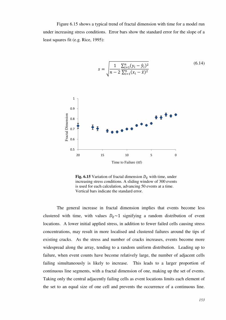
153
Figure 6.15 shows a typical trend of fractal dimension with time for a model run
under increasing stress conditions. Error bars show the standard error for the slope of a
least squares fit (e.g. Rice, 1995):
1w * 2 ∑ 64 * 474q∑ 64 * 74q (6.14)
Fig. 6.15 Variation of fractal dimension with time, under increasing stress conditions. A sliding window of 300 events is used for each calculation, advancing 50 events at a time. Vertical bars indicate the standard error.
The general increase in fractal dimension implies that events become less
clustered with time, with values ~1 signifying a random distribution of event
locations. A lower initial applied stress, in addition to fewer failed cells causing stress
concentrations, may result in more localised and clustered failures around the tips of
existing cracks. As the stress and number of cracks increases, events become more
widespread along the array, tending to a random uniform distribution. Leading up to
failure, when event counts have become relatively large, the number of adjacent cells
failing simultaneously is likely to increase. This leads to a larger proportion of
continuous line segments, with a fractal dimension of one, making up the set of events.
Taking only the central adjacently failing cells as event locations limits each element of
the set to an equal size of one cell and prevents the occurrence of a continuous line.
0.5
0.6
0.7
0.8
0.9
1
05101520
Frac
tal D
imen
sion
Time to Failure (ttf)

154
However, when was calculated for this alternative definition of location
distribution, no significant difference was seen, especially in overall trend (Fig. 6.16).
Fig. 6.16 Variation of fractal dimension with time, under increasing stress conditions. A sliding window of 300 events is used for each calculation, advancing 50 events at a time. Events are defined as the central cell of adjacent simultaneously failing cells. Vertical bars indicate the standard error.
As with the calculation of b, the trade off between windows of a sufficient number of
events for a significant value of , and short enough time period to observe any
variation presents a problem in this analysis. During the early stages of fracture there
are very few events and a large time period must be incorporated to provide a set for
testing which is of equal size to just a single time step much closer to failure. Therefore
any temporal variation that may exist during this initial period is lost. When a sliding
window of equal time period is used for the same data set, a much lower initial fractal
dimension is observed (Fig. 6.17a). However the vast difference in set size makes
comparison of the calculated dimension values difficult. The first window contains just
48 event locations while the final window contains over 1,700. This represents 85% of
the entire array and will therefore naturally produce a very high fractal dimension as the
set tends towards a continuous line. A smaller time window reduces this problem at the
later time scale but reduces the number of events in early time windows even further.
The first fractal dimension in Figure 6.17b is calculated from only 6 events. When a
very small number of events is used, the possible range of cover numbers N(l) in the
box-counting calculation will be reduced, leading to less variation as box size l changes
and hence a very low value for D. Although the range of fractal dimensions varies
0.5
0.6
0.7
0.8
0.9
1
05101520
Frac
tal D
imen
sion
Time to Failure (ttf)

155
considerably between the various methods of calculation (Figs. 6.15 – 6.17), the trend
of an increasing D and a shift towards a random uniform distribution remains consistent
across all cases.
Fig. 6.17 Variation of fractal dimension with time, under increasing stress conditions. A sliding window of equal time period is used for each calculation. Time periods of (a) 20 units and (b) 5 units advance (a) 5 and (b) 3 time steps each calculation. Vertical bars indicate the standard error.
The gradual increase in fractal dimension is generally less evident when models
are run under constant stress conditions. The more typical trend in this case is a
relatively consistent high D-value, showing small fluctuations with time (Fig. 6.18).
This high measurement of again closely approximates the non-fractal condition
1. Figure 6.19 shows the distribution of events in each window used to calculate
the fractal dimensions. The active area shifts with time, but within this area the degree
of clustering appears to remain the same. The concentration of events into localised
0
0.2
0.4
0.6
0.8
1
010203040506070
Frac
tal D
imen
sion
Time to Failure (ttf)
0
0.2
0.4
0.6
0.8
1
0153045607590
Frac
tal D
imen
sion
Time to Failure (ttf)
(a)
(b)

156
areas of activity, rather than distributed throughout the array, can result in a very dense
distribution tending towards a continuous line and high fractal dimension.
Fig. 6.18 Variation of fractal dimension with time, under constant stress conditions. A sliding window of 500 events is used for each calculation, advancing 50 events at a time. Events are defined as the central cell of adjacent simultaneously failing cells. Vertical bars indicate the standard error.
0.5
0.6
0.7
0.8
0.9
1
0 200 400 600 800 1000
fra
cta
l d
imen
sio
n
mid-window event
Mid-Window Event
500 800
Fig. 6.19 Location of events (red) in windows used for calculation of fractal dimensions in Figure 6.18.

157
As would be expected for a non-fractal distribution, the correlation dimension
also remains high (Fig 6.20). The correlation dimension is calculated as the negative
gradient of the log-log plot of 627 against length scale 2 as defined in Equation (6.12).
An example of this linear log-log plot, for the D-values in Figure 6.20 is shown in
Figure 6.21. A good linear fit is observed, however limitations due to the model size
restrict this analysis to only one order of magnitude of length scale 2.
Fig. 6.20 Variation in correlation dimension with time (as described in (6.13)), under constant stress conditions. A sliding window of 300 events is used for each calculation, advancing 50 events at a time. All failed cells are included as event locations.
0.5
0.6
0.7
0.8
0.9
1
0 500 1000 1500 2000
Cor
rela
tion
Dim
ensi
on
Mid-Window Event
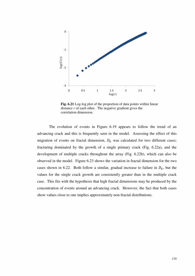
158
Fig. 6.21 Log-log plot of the proportion of data points within linear distance r of each other. The negative gradient gives the correlation dimension.
The evolution of events in Figure 6.19 appears to follow the trend of an
advancing crack and this is frequently seen in the model. Assessing the effect of this
migration of events on fractal dimension, was calculated for two different cases;
fracturing dominated by the growth of a single primary crack (Fig. 6.22a), and the
development of multiple cracks throughout the array (Fig. 6.22b), which can also be
observed in the model. Figure 6.23 shows the variation in fractal dimension for the two
cases shown in 6.22. Both follow a similar, gradual increase to failure in , but the
values for the single crack growth are consistently greater than in the multiple crack
case. This fits with the hypothesis that high fractal dimensions may be produced by the
concentration of events around an advancing crack. However, the fact that both cases
show values close to one implies approximately non-fractal distributions.
-3
-2
-1
0
0 0.5 1 1.5 2 2.5 3
log(
C(r
))
log(r)

159
Fig. 6.22 Evolution of a one-dimensional array of 1,000 cells with time. (a) Failure is dominated by the growth of a single, primary fracture. (b) Multiple cracks grow simultaneously.
Fig. 6.23 Variation in fractal dimension with time, under increasing stress conditions. The two data sets compare for the growth of a single, dominant crack (blue diamonds) and multiple cracks (red squares). Vertical bars show standard errors.
0.5
0.6
0.7
0.8
0.9
1
0 200 400 600 800 1000
Frac
tal D
imen
sion
Mid-Window Event
Failed
Time (a) (b)
Intact
Single crack Multiple cracks

160
The location of events will also clearly be affected by the geometry of initial
cracks in the model. This can differ through the number, length distribution and
location of failed cells. The results shown so far are from models with a random
distribution of initial cracks. To assess the effect of this on the apparent trend of
random uniform spatial distribution of events, D was also calculated for an initial array
containing a fractal geometry of failed cells. Cracks were located using a Cantor dust
set, which is developed through continually removing the middle third of a line segment
(e.g. Falconer, 1990). This set, and therefore the initial trace of cracks in the model, has
a fractal dimension of ln 2 ln 3⁄ , approximately 0.63. The fractal dimensions recorded
remain high, generally in the range 0.7 – 1.0 (Fig. 6.24). A general increase in D
leading up to failure is also often observed.
Fig. 6.24 Variation in fractal dimension with time, under increasing stress conditions and a fractal geometry of initial cracks. Vertical bars show standard errors.
In addition to analysis of the spatial distribution of seismic events, studies have
looked at the temporal clustering of earthquakes (e.g. Vinciguerra et al., 2001).
Occurrence of data in discrete time periods prevents this type of analysis for the one-
dimensional model, because there is no distinction of time lapse between individual
events.
6.3.2 Fault length
As well as investigating the distribution of seismic events, many studies have also
examined the geometry of fault lengths. Bonnet et al. (2001) contains a review of
numerous experimental, numerical and field studies. Various factors have been
0.5
0.6
0.7
0.8
0.9
1
024681012
Frac
tal D
imen
sion
Time to Failure (ttf)

161
identified as affecting the distribution of lengths. In experiments, Krantz (1983)
showed that an increase in applied stress increased the proportion of longer
microcracks. The presence of fluid in specimens can also influence microcrack lengths
(Hatton et al., 1993) with a higher fluid content leading to relatively more small cracks.
Davy et al. (1995) found an exponential distribution of lengths in experiments where
deformation was distributed uniformly, and power law during localised deformation. In
numerical simulations an exponential distribution was observed during early
deformation, becoming power law once fractures began to interact (Cowie et al., 1993).
Power law distributions of fault lengths have also been observed in the field, including
those from a fissure swarm in Iceland (Gudmundsson, 1987), and active surface faults
in the United States (Hatton et al., 1993).
A power law fault length distribution can be described by:
6x7 S x\ (6.15)
where 6x7 is the number of faults of length greater than x. Fault length or area is
related to seismic moment and magnitude (Kanamori & Anderson, 1975). Therefore
this fractal dimension for fault lengths can be related to the magnitude dependent b-
value (e.g. King, 1983; Main 1988):
3u (6.16)
is a constant, usually given by 3 2⁄ for tectonic events or 3 for small events
such as acoustic emissions in the laboratory (Kanamori & Anderson, 1975). Main
(1988) describes the reduction of to a critical value of 1 as a method for failure
forecast. A drop in the exponent is due to the natural tendency for larger cracks to grow
more rapidly and have less chance of arrest. By Equation (6.16), this correlates with the
drop in b-value reported before failure.

162
Crack length distribution was recorded in the model for both constant and
increasing stress conditions, with similar results observed in both cases. Again, the
geometry of initial cracks assigned in the model will have an effect on the development
of the distribution. Figure 6.25 shows a typical log-log plot of the number of cracks
6x7 of length at least x, used for the calculation of fractal dimension . Linearity
generally holds over at least one order of magnitude even when the initially failed cells
are assigned entirely at random. Relatively fast growing primary fractures may account
for the departure from a linear trend at upper length scales although limits of scale in the
model will ultimately restrict the number and magnitude of cracks of a medium to long
length. Boundary problems are also an issue for fault length distributions studied in the
field where the margins of a sampled region are more likely to intersect longer fault
lines, causing censoring effects, or a biased choice of sample region in order to include
or exclude large faults (Bonnet et al., 2001).
Fig. 6.25 Log-log plot of crack length distribution in a one-dimensional array subject to an increasing applied stress. N(l) is the number of cracks greater than length l. The fractal dimension Dl is given by the negative gradient of the linear trend and is calculated over data points where linearity holds (blue diamonds). 0.99.
For the one-dimensional model, was compared to the seismic b-value (Fig.
6.26), which was calculated for magnitudes measured both by the length of adjacent
simultaneously failing cells and the length of adjacent current and existing failures, as
described in Section 6.1.1. The length distribution exponent appears to follow a
general decreasing trend with time, falling to ~1 just prior to failure. Where b is
0
0.5
1
1.5
2
2.5
0 0.5 1 1.5 2 2.5 3 3.5
ln(N
(l))
ln(l)

163
measured by the length of adjacent failing cells (Fig. 6.26a), the two parameters vary in
proportion, as Equation (6.16), until shows a more marked decrease prior to failure.
However, the constant of proportionality gives a value ~ 6 in (6.16), significantly
greater than the expected value of ~ 3. A larger value of reflects a relatively high b
compared to field and laboratory values. is calculated for all cracks in the model and
therefore incorporates the entire history of activity as well as current failures while the
b-value is measured for current events only. By corresponding magnitude values to the
length of current failing cells adjacently linked by existing failures, this encompasses a
measure of previous activity into the b-value and the two parameters b and become
more comparable. Prior to the pre-failure drop-off in the length dimension, ~u as
proposed for small scale faulting (Kanamori & Anderson, 1975).

164
Fig. 6.26 Variation in seismic b-value (blue diamonds) and fractal dimension (red squares) with time, under increasing stress conditions. Magnitude values used to calculate b are derived from (a) the number of adjacent simultaneously failing cells and (b) the number of adjacent current and existing failed cells. Note the change in scale for b.
0
0.5
1
1.5
2
2.5
0
1
2
3
4
5
01234567
Dl
b-v
alue
Time to Failure (ttf)
0
0.5
1
1.5
2
2.5
0
0.5
1
1.5
2
2.5
02468
Dl
b-v
alue
Time to Failure (ttf)
(b)
(a)

165
6.4 Chapter Summary
The seismic b-value associated with tectonic earthquakes is generally found to lie close
to one. The parameter is often observed to be greater than this, b ~ 2 or 3, in areas
surrounding volcanoes. High material heterogeneity and high local stress may
contribute to the anomalously high b-values. A minimum in b-value has been observed
prior to failure at volcanoes and in fracture tests in the laboratory. In the one-
dimensional model, b lies in the range 1 < b < 3, and decreases towards the point of
failure. A similar trend is observed for both increasing and constant stress conditions.
Further work to identify a critical lower limit is necessary to fully utilise the b-value as
a forecasting tool.
Fractal analysis is used to quantify the distribution of fault lengths or earthquake
locations in the field. In the one-dimensional model a fractal dimension describing the
location of all failed cells in the array, and a fractal dimension associated with the
location of events with time were calculated. The former naturally tends to one at the
point of failure. The latter also appears to increase towards a value of one prior to
failure, although the trend can also start from a value as high as ~ 0.9. The log-log
plots used to calculate the dimensions show a good linear fit in all cases. The
distribution of crack lengths in the model also follows a power-law relationship. The
associated fractal dimension is proportional to the seismic b-value over a varying time
interval in the model run. However, the constant of proportionality is greater than that
expected from theoretical results.

166
7. Discussion and conclusions
The aim of this research was to improve understanding of the fracture processes
occurring within a volcano and, thereby, to provide a physical basis for patterns of
accelerating volcano-tectonic seismicity before eruptions. During an interval of weeks
or more, the rate of VT events is commonly observed to increase exponentially with
time and, at least at subduction-zone volcanoes reawakening after centuries of repose,
this increase may evolve into a hyperbolic (faster-than-exponential) increase about two
weeks before eruption (Kilburn, 2003; Kilburn & Sammonds, 2006). The prevalence of
only two trends suggests that rates of crustal fracturing may occur under a small range
of conditions and, consequently, may be amenable to analysis using a model that
requires only a small number of key conditions to be satisfied.
As a result, a numerical model has been developed for which cracking is driven
purely by stress concentration at crack tips, and interaction between neighbouring
cracks. Different external loading conditions were considered, predominantly a constant
applied load and a load that increased gradually with time. In addition, the material
properties of the simulated rock mass could be considered as initially homogeneous or
heterogeneous. Importantly, none of the simulations was required to end in bulk failure.
The simulation has been developed in a simple 1D setting. However, this simple
model manages to capture the essential features of rock cracking and so remained the
focus of this study.
Key results of the 1D simulation are that:
1. Event rates tend initially to increase exponentially with time.
2. Exponential increases in event rate can evolve into hyperbolic trends.
3. Exponential trends are controlled by the activation of an increasing number of
cracks, whereas hyperbolic trends are determined by the interaction of major
cracks that merge together.
4. Hyperbolic trends tend to emerge from a model with initial flaws more closely
spaced than those that produce a purely exponential trend.
5. The preferred precursory trends remain the same, independent of loading
conditions.
6. The magnitude-frequency distributions of model events follow a power-law
relation, consistent with the Gutenberg-Richter law.

167
7. Event rates tend to decrease immediately prior to failure, due to limitations on
remaining intact cells in the array.
8. A small proportion of simulated trends show precursory patterns that differ from
the expected combination of exponential and hyperbolic increases.
The first six results are consistent with the common patterns of VT precursors
observed in the field (Voight, 1988; McNutt, 2005). The agreement between model and
field data supports the view that precursory VT event rates are determined by a
combination of fault activation and of fault growth and linkage (Kilburn, 2003). It also
suggests that the 1D simulation yields realistic results. Accordingly, the final two
results, of a pre-failure drop in event-rate and alternative precursory trends, might yield
insights into additional processes that may be occurring among potential VT precursors
to eruption. Such processes are discussed below, together with their implications for
making decisions during volcanic emergencies.

168
7.1 Model limitations
The 1D model itself has been subjected to a relatively broad sensitivity analysis.
A large-scale analysis would require many more simulations of the model, and was
therefore deemed too computationally expensive. Further work into establishing
properties such as the linearity of output variables or the interaction of input factors may
highlight possible interesting areas for further investigation. Identifying the most
important factors is useful for establishing which commonalities between volcanoes
may lead to similar precursory trends as well as the extent of these similarities.
Information obtained on the sensitivity of the model to the various inputs will improve
with the number of runs made. A Monte Carlo simulation would ideally involve
running a model on the order of 104 - 106 times. Again however, in this case the model
was too computationally expensive to produce such a large amount of data.
The discretisation involved in using a grid-based model for the fracture process
is also an issue that arose in various parts of this research. Continuous modelling
methods such as finite element analysis have seen wide applications across both
engineering and geology problems (e.g. Manconi et al., 2007; Parsons et al., 2006).
This type of approach brings with it numerous other complexities though and again a
balance must be reached between the degree of accuracy required from a model and the
relative simplicity. For the purpose of the research carried out here it was not necessary
to produce an extremely accurate representation of the propagation of a crack, but more
to establish the effects of interaction between two neighbouring cracks and the
subsequent effect of this on an entire population of cracks. The discrete growth of
cracks within the model also affected the analysis of seismic event magnitude
distributions. A more varied distribution of magnitudes could be attained by dividing
cells into smaller segments, and introducing a stochastic element of how many of these
segments are to be used for a magnitude calculation. However, even though it gives a
limited range, it is useful to have a measure of magnitude that can be directly linked to a
physical parameter in the model. In addition, the grouping of recorded magnitudes in
the field also leads to a discrete range of values.
The one-dimensional array used to represent the progressive failure of the
edifice is of course a vast simplification of the modelled process. As described in
Chapter 4, the interaction and coalescence of fractures and faults within host rock of a
volcano will occur by shear faulting between neighbouring, non-aligned fractures rather

169
than simple tip-to-tip extension. Accordingly the model represents the development of
failure within the edifice rather than the formation of a purely extensional fracture. The
model assumes magma ascent as a passive action once the edifice is sufficiently
fractured so as to no longer create a limitation on the movement of magma. However,
little mention has been made of the proposed subsequent ascent of magma to the
surface, and a much greater understanding of this must be developed in order to present
a complete model of eruption mechanics. In particular, the feedback process between
the propagating magma and host rock deformation is an important factor in the physics
of magma ascent. Once magma begins its ascent, pressure in the magma chamber would
be expected to fall. As a source of loading on the surrounding host rock, this may in turn
lead to a reduction in the rate of cracking and seismicity. This drop-off in seismicity
prior to eruption is observed in the field and is represented in the model by a
redistribution, or loss of stress due to a limit on the number of remaining intact cells.
This model of edifice failure and magma ascent assumes that once a connected
network of faults and cracks has formed, magma will follow its course to the surface.
The creation of a fully connected conduit, linking a magma chamber to the surface is
again a highly simplistic concept. Field observations suggest that magma-driven cracks
propagate in a direction of principal stress and do not necessarily follow cracks and
faults that already exist within the edifice. It must therefore be noted that while the 1D
model reproduces recorded precursory seismicity by focusing on the interactions of a
network of cracks, it cannot necessarily be assumed that this process leads directly to
the creation of a conduit for magma ascent. Feedback and interplay between the two
processes may instead be considered. Shear faulting and the coalescence of fracture
networks may occur radially throughout the edifice, around a central axis of
deformation, due to the loadings described previously. The 1D model then still
represents a progression towards, and a measure of failure. However, the failure is
representative of, rather than a direct cause of the creation of a pathway for magma
ascent. Once the magma chamber ruptures, propagation of a magma-filled crack may
still cause shear faulting or cracking within the surrounding rock due to redistribution of
pressure or of geothermal fluids and volatiles. The interaction between fluid movement
and fracturing is discussed in further detail in Section 7.2.3. Eventually this type of
cracking and faulting, and therefore the related high-frequency earthquakes, falls away
as pressure is released and the seismicity observed becomes lower in frequency,
representative of the movement of magma through the volcano.

170
Further studies are required to explore this idea in more depth and would need to
focus on details such as the utilisation of accurate location and source mechanisms of
precursory volcano-tectonic earthquakes, and field, experimental and modelling
approaches to understanding the interplay between faults and dykes within volcanoes.

171
7.2 Applications of the model to investigating the behaviour of
volcanoes
The results of the 1D model are consistent with field observations that volcanic
eruptions are commonly preceded by exponential increases in VT event rate with time.
They also show that exponential trends can evolve naturally into hyperbolic increases in
VT event rate. Such agreement between field and model results suggests that the model
has captured the essential features of fracturing at volcanoes. An immediate practical
implication is that the model supports interpretations of VT eruption precursors in terms
of the activation and interaction of a population of fractures in subvolcanic crust and
volcanic edifices. Two further implications are (1) that the less-common variations in
model event rate that do not follow exponential or hyperbolic trends may also have
analogues among the full spectrum of field precursors, and (2) that the model may be
extended to investigate conditions for non-eruptive fracturing at volcanoes. The last two
implications are of special interest at volcanoes that show unrest after long repose,
because these are the volcanoes for which the least field data are available.
Consequently, it is possible that some of the less-common trends in the model have yet
to be identified in the field. The following sections therefore discuss how the numerical
model might be used to guide future investigations into patterns of volcanic unrest.
7.2.1 Decreases in event rate before eruptions
A recurring feature in the model is the drop-off in event rate observed immediately prior
to bulk failure. This has been attributed to the limit on remaining intact cells once the
whole array is nearing failure. However, it is interesting to consider whether this kind
of effect may be related to physical processes occurring in the field, due to release of
magmatic pressures, either before eruptions or during false alarms. This section
addresses pre-eruptive decreases; false alarms are considered in Section 7.1.2.
The 2000 eruption of Usu in Japan (Zobin et al., 2005) and the 1994 eruption at
Popocatepetl in Mexico (De la Cruz-Reyna et al., 2008) provide two examples of pre-
eruptive decreases in VT event rate. At Mt Usu, following an acceleration in seismic
event rateover a period of approximately three days, the rate then began to decline, with
the onset of eruptive activity occurring more than 12 hours after the peak in seismicity
(Zobin et al., 2005). The model developed here presents the ascent of magma as an
entirely passive process once an open pathway has been created. In addition to the

172
limits on intact cells, it is therefore also possible to imagine a time-lag between the
formation of this open fracture network and the first emergence of magma at the surface
determined by the rate of magma ascent. The failure forecasting methods described
throughout this thesis suggest that the onset of activity coincides with the peak point of
the observed precursor. However, it is also possible to imagine and to explain a
scenario where although the forecasting method may correctly predict the time of
failure, a decrease in the precursor may be observed prior to this.
A longer period between a swarm of seismic activity and the onset of eruption
has been observed in the field. De la Cruz-Reyna et al. (2008) describe four phases of
activity leading up the eruption of Popocatepetl in 1994, activity that followed almost
70 years of rest at the volcano. The increase in seismicity recorded in the years to
months before the eruption are attributed to a series of magmatic injections, thermally-
induced cracking and volumetric increase in the density of cracks and fractures caused
by a concentration of stress. This latter process produced the type of acceleration in
volcano tectonic activity analysed in this research. Extrapolation of a hyperbolic fit to
the seismic energy released during the first three phases of activity provides a good
forecast to the onset of the eruption. However, the observed acceleration in seismic
activity shows a significant decline in the months prior to the eruption and the
distribution of hypocentres becomes much more greatly dispersed. De la Cruz-Reyna
et al. (2008) speculate that this final stage of activity may be indicative of a
redistribution of built up stress throughout a greater volume of host rock as the
effectively closed volume experiencing the acceleration in seismicity and fracturing is
no longer able to maintain it. In essence this is similar to the process causing a drop in
event rate in the one- and two-dimensional models, where there is a limit in the ability
of the array to maintain the level of failing cells.
7.2.2 False alarms
The growth of cracks in the one-dimensional array, as well as in rock in the laboratory
and field, creates a positive feedback. Stress intensity at the crack tip is an increasing
function of the size of the crack. Therefore with nothing to prevent further growth, once
a crack begins to extend, it grows rapidly until the entire array, block of material or
volcanic edifice has failed. In nature however, this is clearly not the case. There are
many more intrusion episodes at volcanoes that do not lead to the eruption of magma at
the surface, than those that do (e.g. Gudmundsson and Philipp, 2006). Therefore for a

173
model to accurately describe the failure mechanism that occurs within a volcano, it must
be possible for an extending crack to arrest before bulk failure is reached. This model
may then help to explain the still poorly understood mechanism creating false alarms at
volcanoes.
Fig. 7.1 Event rate with time for a one-dimensional array subjected initially to an increasing stress, which is then reduced by 50% and held constant. The dashed line shows the point at which stress is reduced. The event rate continues increasing until bulk failure of the array is reached.
Results shown in the thesis so far have focused on those cases when the model
array fails. In the case of an increasing stress this will always eventually occur. For
constant stress conditions, whether or not the array fails will depend on the chosen level
of applied stress. In terms of improving understanding of false alarms at volcanoes, the
cases when the model does not fail can also be of interest. In many cases, the location
of initial cracks within areas of relatively high fracture toughness and a low level of
applied stress results in a cessation of activity in just a few time steps. Under a
randomly distributed fracture toughness, it was also observed that once a relatively large
proportion of the cells had failed, it was likely that the array would progress to failure.
Often, even if a drop in the applied stress was introduced, the density of fractures was
sufficient to maintain the necessary degree of stress concentration at crack tips and to
sustain the positive feedback of crack growth (Fig. 7.1). However, there are also a few
cases when the event rate does die down after a drop in the applied stress. Figure 7.2
shows an example of two different model runs in which the applied stress is decreased
0
100
200
300
0 20 40
Eve
nt r
ate
Time

174
at the point indicated. In one case the model continued fracturing until the entire array
had failed. In the second case, after an initial continuation of failing the event rate died
down and finally stopped, with intact cells still remaining in the array. The similarity of
the two trends, before one goes on to fail and one returns to equilibrium highlights the
potential difficulty of distinguishing between these scenarios in the field. If the primary
source of stressing in a volcano is the overpressure of a magma reservoir, the release of
some of this pressure, for example in the form of an intrusion event, may lead to a
relaxation, or at least redistribution of the regional stress. The one-dimensional model
demonstrates that in such a scenario, increased seismic activity may eventually die
down without the emergence of magma at the surface.
Fig. 7.2 Event rate with time for two separate runs of the one-dimensional model. The models are subjected initially to an increasing stress, which is then reduced by 50% and held constant. The dashed line indicates the point at which stress is reduced. After this drop, fracturing continued in one run of the model until bulk failure of the array (blue diamonds), while in the second run the event rate eventually died down and the model remained in an intact state (red triangles).
As well as a reduction in stress and therefore stress intensity, the second factor
that may lead to the arrest of a propagating network is an increase of critical fracture
toughness. A random fracture toughness distribution means that even if a propagating
crack runs into a region of relatively high fracture toughness, it is likely that this region
0
40
80
120
160
0 20 40 60
Time
Eve
nt r
ate

175
will cover no more than one or two cells distance from the crack and therefore if the
crack is long enough its range of influence may also reach to the less resistant cells
beyond. Therefore once longer cracks have formed it is very difficult to prevent failure
of the entire array. While mechanical properties of rock making up a volcano are likely
to be highly heterogeneous, with stiffness of different rocks ranging over four or five
orders of magnitude (Gudmundsson & Philipp, 2006), it is also reasonable to imagine
that there will be some degree of local homogeneity in the layers making up the edifice.
Gudmundsson and Philipp (2006) found that a dyke intrusion leads to an eruption only
if a homogeneous stress field exists through the edifice. They used finite element
analysis to investigate the effect of layers with various mechanical properties on the
propagation of a dyke and found that while stiff layers favoured propagation, soft layers
tended to arrest the dyke. Generally, a dyke reaches the surface by stress-field
homogenisation, a process that reduces the stress difference between layers of host rock.
When a dyke reaches the contact between adjacent layers it may become arrested or
spread laterally to form a sill before either arresting or continuing its vertical
propagation (Gudmundsson, 2003).
A layering of fracture toughness is a very simple constraint to build into the
existing crack interaction model. In the one-dimensional case, the only option for a
crack approaching a contact between two layers is to arrest or continue vertical
propagation. However in two dimensions, with an adjustment of propagation rules
within the array it would be possible to allow for horizontal spreading of a crack. In the
case of a fluid filled crack, discussed below, this would then form a sill that in turn
would alter the surrounding stress field further. This type of layered model could be
developed into a stochastic tool for forecasting the proportion of intrusive to eruptive
episodes at a volcano. Running numerous simulations, varying the distribution of initial
cracks or external stress conditions provides a count of how many instances the array
progresses to failure and how many times a swarm of activity occurs but then dies down
without bulk failure. This type of study would give an indication of how often non-
eruptive swarms might be expected at a volcano. It is also essential to be able to
identify which these swarms are. Analysis of observable parameters such as earthquake
locations or event rate trends may identify potential tools for such a forecasting
capability. For example, with the potential for accurate event location it may be
possible to identify a switch of location of concentrated activity as a major propagating
crack becomes arrested.

176
7.2.3 Modelling intrusions
Failure of the one-dimensional model is based solely on fracture mechanics of a brittle
material and assumes that it is this failure of a volcanic edifice that is the controlling
factor on the ascent of magma to the surface (Kilburn, 2003). As discussed in Section
7.1, an interesting further development of the model would be to consider the effects of
magma movement on the fracture network, once created, whether within or removed
from the network. It is widely accepted that there are significantly more intrusion events
at volcanoes, involving the propagation of a magma-filled dyke, than there are
eruptions. This is therefore an important area of research and many numerical,
empirical and theoretical studies have been carried out on the dynamics of fluid filled
cracks and of dyke propagation. This section looks at the role of fluid within the
fracture network, although this may be geothermal fluids rather than magma.
Allowing for fluid movement within the model is likely to introduce complex
interactions with seismic activity. Rivalta and Dahm (2004) describe this interaction in
a heavily fractured edifice. Dyke intrusion causes further cracking of the host rock,
which in turn becomes weakened allowing for further propagation of the dyke. This
type of positive feedback, leading eventually to bulk failure, has been previously
described in terms of crack length dependent stress intensity factors. The effect of a
propagating dyke on surrounding cracks is also akin to the interaction effects in the one-
and two-dimensional models. Reaction of surrounding material to a fluid filled crack
will depend on properties of both agents, such as the mechanical properties of the host
rock and the buoyancy or volatile content of the magma. Roper and Lister (2007)
described a fracture toughness parameter that incorporates the resistance to viscous flow
as well as fracture. Along the length of a dyke, away from the tip, induced strains are
on the order of the dyke’s width to length ratio and are therefore generally small (Rubin,
1995).
If an intrusion of magma does not lead to enhanced fracturing of the host rock, it
will still cause an increase in size of the channel it enters and can therefore result in
observable ground deformation at the surface (Rubin, 1995). Two dimensions allow a
factor of area change to be incorporated into the model, which can be extrapolated to
look at volume change and deformation associated with failure in the edifice. Along
with seismic activity, ground deformation is another promising tool for eruption
forecasting and when taken in partnership with seismicity can help to create a clearer
picture of activity beneath and surrounding a volcano. Technological advances in this

177
area have been great over the past few decades with many studies on volcanoes now
using techniques involving InSAR (Interferometric Synthetic Aperture Radar) or GPS
(e.g. Baer et al., 2008; Palano et al., 2008). Ground deformation studies can be useful in
forecasting eruptions, identifying dyke intrusions and also for monitoring magma
movement during an eruption (Kohno Y. et al., 2008).
Pressure source models translate volumetric change observed on the surface to
sub-surface changes within the Earth’s crust. Mogi’s (Mogi, 1958) magma intrusion
model is often used to correlate a volume change in a magma chamber to ground
deformation. This model assumes a spherical magma body at depth, within an elastic
body of country rock. It has also been suggested that mechanical properties of rock
have a significant effect on displacements and deformation and that therefore
heterogeneity is an important factor to allow in such a model (Manconi et al., 2007).
The two-dimensional model described in chapter 7 was developed to consider the
percolation of a damaged array and the properties of the resulting network. However,
this model could be expanded further to also incorporate intrusions of magma into the
fracture network and the subsequent increase in area of the array. The simplicity of the
grid-like model allows for features such variation in area change with material
properties. Clearly further complexities would also be necessary within such a model to
incorporate local stress variation due to intrusions and pressure sources (Gudmundsson,
2002), and the effects of an expanding grid space. Intrusions may also have a more
global effect across the grid. Toda et al. (2002) suggested a linear relationship between
stressing rate induced by an intrusion event and remote seismic activity. A separate
study on the same intrusion event in the Izu Islands, Japan uses this relationship to
propose a method for establishing whether dyke expansion is occurring as a passive
reaction to fracturing or due to the intrusion of magma (Rivalt & Dahm, 2004).
Modelling a fluid flow involves a much greater degree of complexity than is
currently built into the fracture model. However, just by introducing additional stress
perturbations brought about by magmatic intrusions and allowing these effects to
propagate in such a way as to be representative of a viscous flow, the first order effects
of dyke intrusions on a fracture network can be approximated. Allowing for volume
change in the model as these intrusions occur could also be useful in providing a basic
link between observed ground deformation and seismicity with activity caused by
magma movement within a volcano.

178
7.2.4 Time-dependent rock failure
Greater complexity may also be built into the model by considering a time-dependent
element, within the discrete time steps of stress redistribution. Currently each cell can
exist in one of only two states, failed or intact. In theory a cell can remain at a very low
level of stress right up until the time step during which it fails, as a major crack extends
close enough to significantly increase the stress intensity of the cell. Alternatively, a
cell adjacent to a crack tip may have a fracture toughness great enough to prevent the
crack propagating until either an increase in remotely applied stress or a neighbouring
crack advances close enough to cause interaction effects. In the latter case, although the
cell does not fail immediately, it is nevertheless subject to a force that it would not feel
if were completely isolated. Attempting to model if and when this cell may fail, and the
crack propagate involves may introduce the concept of sub-critical crack propagation or
use of a damage parameter. Sub-critical crack growth describes the extension of a crack
at a stress intensity below its critical value and can be influenced by factors such as
temperature, pressure as the presence of corrosive fluids (Atkinson, 1984), all of which
can apply to a volcanic setting. Introducing the theory of damage mechanics allows the
fracture of rock to be dealt with in a framework of continuum mechanics.
Main (2000) uses the concept of damage mechanics to look at time-dependent
stages of creep in the Earth’s crust, and to explain the foreshock and aftershock
sequences of earthquakes described by Omori’s law. Based on the constitutive
equations of time-dependent crack growth, Main’s model incorporates both a positive
and negative feedback on rock failure, where local negative feedback occurs through
strain hardening mechanisms. The occurrence of stress shadows will be discussed again
in the following section. These various concepts of time-dependence can be built into
the model by recording in essence a damage parameter for each intact cell. This may
incorporate the number of time steps a cell is exposed to a stress intensity greater than
the background remote stress, which would allow only cells surrounding a crack tip to
experience any extent of damage, or a function of the ratio of stress intensity to fracture
toughness thereby affecting all intact cells.
Modelling the host rock as a visco-elastic material would also create time
dependent failure. The fracture mechanics currently applied to the model assumes
brittle failure of rock is producing the volcano tectonic events recorded prior to
eruption. Long period seismicity that becomes more common after the onset of
eruption is associated with the movement of magma rather than brittle failure. Recent
179
studies suggest however that fracturing may not be confined to cool, brittle rock only.
Tuffen at al. (2008) carried out high temperature fracture tests on lavas to investigate
the possibility of seismogenic faulting along conduit walls, and within lava domes and
erupting magma. Waveforms produced by the laboratory experiments showed both
similar onset patterns and frequency content to volcano tectonic earthquakes. Looking
instead at long period events, Neuberg et al. (2006) model the brittle-ductile transition
of magma within the conduit where the low frequency seismicity is caused by the build
up of shear stresses along the conduit wall as the magma ascends.
Seismogenic faulting of magma at shallow depths, either along the conduit walls
or in lava domes, will generally only occur once a pathway to the surface has been
largely created. It is therefore still reasonable to suppose that seismic activity used in
the failure forecast methods described in this thesis can be assumed to come from the
failure of host rock and the opening of a new fracture network. However as discussed
above, the one-dimensional model of precursory seismicity produces a fall in volcano
tectonic style events immediately prior to failure, and any attempts to improve the
representation of the fracture and faulting development during this interval should take
into account the possibility of high-frequency swarms produced by ascending magma
itself. The effects of temperature on the fracture process at greater depths can also be
incorporated into the existing model framework by looking at the effect of temperature
change on fracture toughness.
It should also be noted at this point that many potential additions to the fracture
model may become irrelevant when considering its ultimate function. The failure
forecast method looks at the change in event rate and therefore requires data such as the
number of events per hour or per day. Equally field data will often be presented in this
way. Therefore the ability to model the time of events to a greater and greater accuracy
becomes irrelevant. The discrete time scale used in the one-dimensional model
reproduces observed data and is therefore essentially fit for purpose. Adding further
complexities may not necessarily add any further utility to the model.

180
7.3 Modelling rapid changes in loading conditions
The fracture model has thus far been run under conditions of either a constant applied
stress, using only the positive feedback created by the extension of cracks to induce
further failure in the array, or a gradually increasing remote stress. When considering
the mechanisms behind arrested failure and false alarms, a sudden decrease in stress was
also applied. An area of potential future work would be to look at the application of a
sudden, relatively large increase in ambient stress. Stress within a volcano is generally
assumed to build up gradually by processes such as the increase in pressure within a
magma chamber, or the exsolution of gases from ascending fluids. However, volcanoes
can also react to dynamic and particularly static stress changes brought about by
tectonic earthquakes. In recent years the idea of the transfer of stress during
earthquakes, and the potential for the triggering of a volcanic eruption has been well
publicised. It has been suggested that such triggering can cover time intervals from
seconds to decades and distances from metres to thousands of kilometres (e.g. Freed,
2005). Static stress changes can lead to a triggered earthquake weeks or even years
following an initial event. Effects diminish with distance from the slipped fault by
some inverse function (Steacy et al., 2005). The one-dimensional model already
incorporates a triggering mechanism in the sense that interaction between cracks can
adjust local stress intensity. It is also possible to investigate the potential for interaction
effects on a much larger scale.
It is very difficult to identify a definite causal relationship between a tectonic
event and a subsequent volcanic eruption. There are several cases reported however
where some correlation has been suggested between tectonic and volcanic activity (e.g.
Cerro Negro, Nicaragua, La Femina et al., 2004; Vesuvius, Italy, Marzocchi et al.,
1993; Merapi, Indonesia, Walter et al., 2007 ). A volcanic eruption may be induced by
a variety of changes in the magma reservoir or conduit with, for example, both
compression or dilation of a magma chamber capable of initiating volcanic unrest
(Selva et al., 2004).
Coulomb stress transfer is often used as a measure of the increase or decrease in
proximity to failure of a fault, following a change in regional stress (Toda et al., 1998).
Studies using Coulomb stress change have been used to highlight potential risk areas for
future earthquakes. McCloskey et al. (2005) calculated stress changes brought about by
the magnitude 9.1 Sumatra-Andaman earthquake in December 2004. They highlighted

181
the contiguous Sunda trench as a real risk for future slip, with stress on the northern part
of this segment calculated to have increased by 5 bars. Indeed this section did rupture
in March 2005, creating a magnitude 8.7 earthquake and claiming the lives of about
2,000 people (Nalbant et al., 2005). This highlights the potential of stress triggering and
in particular Coulomb stress forecasts in the area of seismic risk analysis. A similar
style of forecasting tool, applicable to the effects of a tectonic earthquake on the
increased probability of eruption at a volcano, would be a useful aid in disaster
management.
Within the one-dimensional fracture interaction model it is possible to represent
a step increase or decrease in the applied stress to represent a static stress change.
Applying a Monte Carlo method, with parameters for mechanical properties suitable for
the volcano in question, it is possible to model the conditions under which an
earthquake may trigger an eruption, and the probability of this occurrence. With a more
complex version of the model allowing for incorporation of magma and fluid
movements, the effect of dynamic or static stress changes on the magma reservoir can
also be modelled.

182
7.4 Decision-making during volcanic emergencies
A second aspect of the fracture model that could be developed is the investigation of
potential warning times before an eruption. This would incorporate existing work on
the characteristic time scales of exponential trends, the emergence of hyperbolic trends,
and the relative probabilities of an eruption or false alarm. An important application is
in the decision making procedure for civil authorities in the event of a volcanic crisis.
Probability plays a major role in eruption forecasting. This role has often
proved to be quite controversial in terms of disaster mitigation and management. First
is the problem of translating data such as observed precursors, historical knowledge and
expert opinion into one figure representing the likelihood of the nature, location or time
of the onset of activity. Once armed with this information, the next problem is what to
do with it. For example, how high should the probability of activity be before an
evacuation is called? This choice is ultimately weighted against the problem of how
long a time interval is required for evacuation. If a large population lives on or around a
volcano, it is vital that sufficient warning be given to allow a full and orderly
evacuation. The overall decision in calling for an evacuation is therefore a trade-off
between the relative certainty of an eruption occurring, and the time needed for a
complete evacuation. Often this decision is made on a subjective basis, during the
developing volcanic crisis. Such decisions may be aided by prior knowledge of the
expected time scale of precursory activity.
Marzocchi and Woo (2007) proposed a probabilistic, cost-benefit strategy to
provide a quantitative decision framework in a volcanic crisis. They look at a case
study of an eruption at Vesuvius, Italy and the risk posed to the highly populated Bay of
Naples, and the cost of mitigation measures against an acceptable level of risk for
society. The decision is basically to evacuate or not to evacuate. In this economical
framework this decision is made taking into account the potential cost of each action.
The discrete decision-making applied in this study assumes that sufficient time
will be available to perform a full evacuation. An added complexity to the model is the
more realistic continuous relationship between the loss risk and the time available for
evacuation. A concept of the probable time frame available for evacuation is clearly
also an important factor in the decision making process. Using theoretical models of
time to failure forecasts can provide an upper limit on the potential time available for
evacuation. If a hyperbolic increase is expected in precursory seismic event rate, an

183
upper and lower limit for time to failure is given by the proposed range in gradient
limits, derived from physical and mechanical properties of a volcanic edifice. However,
clearly this time interval must then be adjusted for the time already elapsed from the
start of the increasing event rate to the point at which the trend is recognised. Similarly,
the concept of the characteristic timescale in an exponentially increasing event rate can
provide an estimate of time to eruption, again shortened by the time taken to identify the
event rate trend and timescale. For the purpose of creating a decision making tool
before the event of a potential crisis, it is useful to have some information on the
probable chances of the various different timescales proposed by the theoretical models,
and previous records of activity.
A Monte Carlo simulation of possible precursory activity would provide just
that. The simulation of 300 runs described in Chapter 4 shows the range in output
distributions from a variation in several different input factors. By allowing for
different distributions of the various input factors, this type of simulation can be made
as general or specific as required, and can show the potential variation in output trends
even for a relatively constrained problem. As well as providing a range, the large
number of runs also provides a valuable indication to the relative likelihood of
occurrence of each of the outputs (Fig. 7.3). In particular, it can provide a probability
distribution of the time to failure and this information could then be used to augment the
respective cost and benefit associated with decision-making in the time of a crisis.

184
Fig. 7.3 (a) Four characteristic exponential trends and (b) the frequency of exponential sequences from the Monte Carlo simulation described in Chapter 4 when grouped with the closest characteristic trend.
Eve
nt r
ate
(b)
(a) Time
Rate constant
Freq
uenc
y

185
7.5 Alternative methods for forecasting eruptions
Alternative forecasting methods can also be incorporated to aid in identifying between
precursory accelerations in seismicity and non-eruptive swarms. In the event of an
approaching volcanic crisis, applying a suite of techniques to accumulating observations
will inevitably provide more information on which to base forecasts and decisions. In
addition to seismic event rate, various other methods built from failure of the volcano
have been developed. For example, the volume of rock that must be fractured for an
eruption to occur can provide a characteristic threshold for the seismic energy released
(De la Cruz-Reyna, 2008). Cumulative Benioff strain was used to forecast eruptions at
Mount St. Helens following the cataclysmic May 1980 eruption (Malone et al., 1983).
The longer the inter-eruption interval, the longer the precursory increase in seismic
energy release. This relation was therefore suggested as a method for forecasting the
time of approaching eruptions. Zobin and Jiménez (2008) suggested a relationship
between the length of precursory seismicity and the magnitude of the eruption at
volcanoes erupting after more than 100 years quiescence. A longer period of seismicity
was associated with a lower VEI index at six different volcanoes studied.
Many methods that appear to provide a promising tool have only been tested in
producing hindcasts, with few reports of successful, true forecasts of the onset of
volcanic activity. It has also been suggested that in a time of crisis it would be very
difficult to distinguish between the type of seismic signals incorporated into the failure
forecast methods. By their very nature eruptions following a long repose interval
happen relatively rarely. Their activity is often explosive in nature, producing eruptions
of VEI 5. Eruptions of VEI 5 are expected roughly once a decade, while those with
VEI 6 only slightly more often than once a century (Woo, 1999). Therefore there is a
lack of field data to test such forecasting tools against and in this situation the use of
empirical and numerical models, such as that developed here, becomes vital in order to
identify the most plausible models to apply in forecasting these relatively infrequent,
but highly hazardous eruptions.
186
7.6 Conclusions
The one-dimensional crack model is based on a fracture mechanics representation of
failure within a volcano. It produces results consistent with field observations,
especially before eruptions at subduction-zone volcanoes reawakening after long repose.
Accordingly, the model supports interpretations of VT eruption precursors in terms of
the activation and interaction of a population of fractures in subvolcanic crust and
volcanic edifices. In particular, the model suggests that:
• Exponential trends are controlled by the activation of an increasing number of
cracks, whereas hyperbolic trends are determined by the interaction of major
cracks that merge together.
• Variations in the application of a remote stress field have a lesser effect on
failure rate than the local ratios of stress intensity to fracture toughness.
• Failed eruptions may be caused by a redistribution of stresses, or by a
heterogeneous edifice.
• Characteristic timescales associated with failure rate are indicative of the volume
of rock to fracture. In the absence of definite criteria for failure forecasting, the
characteristic timescale can provide a limit on the expected time to failure.
• A Monte Carlo simulation of the failure of a volcanic edifice can provide
probabilistic data for an expected time to failure, as well as highlighting possible
precursory trends to be observed before future eruptions.
To build on these results, future studies can extend the model to two and three
dimensions, develop analyses of non-eruptive accelerations in VT event rate, and
investigate the behaviour of deformation parameters in addition to event rate alone. In
combination, such studies will help to improve interpretations of volcanic unrest and, as
a result, will also enhance decision-making procedures during volcanic emergencies.

187
Appendices
Mathematica code to run 1D model of crack interaction:
<< Statistics`DescriptiveStatistics`
<< Statistics`ContinuousDistributions`
gaussdist = NormalDistribution[0, 1];
(* user input for length of array *)
n = Input["Enter number of elements"];
(* user input for initial stress and stress increase *)
initApp = Input["Enter initial value of remote applied stress"];
appStep = Input["Enter increment value for applied stress per step"];
(* user input for the area of each cell as used in the magnitude
calculations *)
area = Input["Enter the area of each element. Area of
1/10,000 corresponds to the failure of a single element being a
zero magnitude event"];
(* Creates Random Walk of n elements *)
strengthinit = ;
For[i = 1, i ≤ n, i++,
AppendTo[strengthinit, Apply[Plus, Table[Random[gaussdist],
n]]];
];
(*Shift values to make all toughnesses initially positive*)
strengthinit = strengthinit - Floor[Min[strengthinit]] + 1;
(* produces stiff and soft layers *)
(*topStiff = Take[Sort[strengthinit], -100];
topSoft = Take[Sort[strengthinit], 50];
For[i = 6, i ≤ 9, i++,
strengthinit =
ReplacePart[strengthinit, topStiff, Table[x, x, i*100 +
1, i*100 + 80], Table[Random[Integer, 1, 100], 80]];
strengthinit = ReplacePart[strengthinit, topSoft, Table[
x, x, i*100 + 81, (i + 1)*100], Table[
Random[Integer, 1, 50], 20]];
];*)
bvalEvolve = ;
dEvolve = ;
dErr = ;
maxScale = ;
dEvolveMesh = ;
dErrMesh = ;
maxScaleMesh = ;
eventEvolve = ;
eventEvolveEpicentre = ;
invEventEvolve = ;
crackEvolve = ;
eventListBnk = ;
eventListBnkJoin = ;
magLst = ;
magLstJoin = ;
magLoc = ;
magLocJoin = ;
newFailedLst = ;
lgthLst = ;
stressIntensityTipEvolve = ;
stressToughTipEvolve = ;

188
stressIntensityEvolve = ;
stressToughEvolve = ;
faultTrace = ;
time = 1;
(* module records length and mid - point of adjacent failed cells for
calculations *)
(* returns lists (lgth of new failures + midpoint, lgth of connected
new failures + midpoint, lgths of all failed cells *)
crackSites[x_, y_] := Module[newFailed,
newFailed = x;
newFailedJoin = x;
allFailed = y;
allFailedCalc = y;
totList = ;
totListJoin = ;
totListAll = ;
crackSt = Min[Position[newFailed, 0]];
relLoc = crackSt;
For[i = 0, crackSt ≠ Infinity, i++,
newFailed = Drop[newFailed, crackSt - 1];
crackEnd = If[Min[Position[newFailed, 1]] ==
Infinity, Length[newFailed] + 1, Min[Position[newFailed, 1]]];
crackLgth = crackEnd - 1;
AppendTo[totList, crackLgth, relLoc + (crackLgth -
1)*0.5];
newFailed = Drop[newFailed, crackLgth];
crackSt = Min[Position[newFailed, 0]];
relLoc = relLoc + crackLgth - 1 + crackSt;
];
(* includes length of original crack if both tips
propagate, rather than two new growths *)
crackStJoin = Min[Position[newFailedJoin, 0]];
relLocJoin = crackStJoin;
For[i = 0, crackStJoin ≠ Infinity, i++,
newFailedJoin = Drop[newFailedJoin, crackStJoin -
1];
allFailed = Drop[allFailed, crackStJoin - 1];
crackEndJoin = If[Min[Position[newFailedJoin,
1]] == Infinity, Length[newFailedJoin] + 1,
Min[Position[newFailedJoin, 1]]];
crackLgthTemp = crackEndJoin - 1;
newFailedJoin = Drop[newFailedJoin, crackLgthTemp];
allFailed = Drop[allFailed, crackLgthTemp];
endAll = If[Min[Position[allFailed, 1]] == Infinity,
Length[allFailed], Min[Position[allFailed, 1]]];
newFailedCovered = Max[Position[Take[newFailedJoin,
endAll], 0]];
If[newFailedCovered == -Infinity,
crackLgthJoin = crackLgthTemp;,
crackLgthJoin = crackLgthTemp +
newFailedCovered;
newFailedJoin = Drop[newFailedJoin,
newFailedCovered];
allFailed = Drop[allFailed, newFailedCovered];
];
AppendTo[totListJoin, crackLgthJoin, relLocJoin +
(crackLgthJoin - 1)*0.5];
crackStJoin = Min[Position[newFailedJoin, 0]];
relLocJoin = relLocJoin + crackLgthJoin - 1 +
crackStJoin;

189
];
(* records all crack lengths *)
crackStAll = Min[Position[allFailedCalc, 0]];
For[i = 0, crackStAll ≠ Infinity, i++,
allFailedCalc = Drop[allFailedCalc, crackStAll - 1];
allFailedEnd = If[Min[Position[allFailedCalc, 1]] ==
Infinity, Length[allFailedCalc] + 1,in[Position[allFailedCalc,
1]]];
crackLgthAll = allFailedEnd - 1;
AppendTo[totListAll, crackLgthAll];
allFailedCalc = Drop[allFailedCalc, crackLgthAll];
crackStAll = Min[Position[allFailedCalc, 0]];
];
Return[totList, totListJoin, totListAll]
];
(* module adjusts stress intensity around crack tips according to
crack length and distribution of surrounding cracks *)
(* returns (state, stress intensity, tghness) data with stress
intensity adjusted around crack tips *)
kfacInt[x__] := Module[j, jBnk, lgth,
data = x;
For[s = 1, s ≤ n, s++,
AppendTo[data[[s]], , ];
data[[s]] = Flatten[data[[s]], 1];
];
j = 0;
jBnk = ;
lgth = 1;
For[l = 1, Min[Position[Drop[data, Min[j + lgth - 1, n]],
0, _, _, _, _]] ≠ Infinity, l++,
j = j + lgth - 1 + Min[Position[Drop[data, j + lgth
- 1], 0, _, _, _, _]];
If[MemberQ[jBnk, j], jInd = 1, jInd = 0];
lgth = 1;
For[i = 1, j + i ≤ n && MatchQ[data[[j + i]], 0, _,
_, _, _] && i < n, i++,
lgth = lgth + 1;
];
(* adds distance and length to all cells within half
- crack - length distance below current tip *)
For[k = 1, k ≤ Floor[lgth/2] + 1 && jInd == 0, k++,
If[j - k > 0,
If[data[[j - k, 1]] ≠ 0,
AppendTo[data[[j - k,
4]], k, lgth];
];
];
];
(* adds distance and length to all cells within half
- crack - distance above current tip *)
For[m = 1, m ≤ Floor[lgth/2] + 1 && jInd == 0, m++,
If[j + lgth - 1 + m ≤ n,
If[data[[j + lgth - 1 + m, 1]] ≠
0,AppendTo[data[[j + lgth - 1 + m, 5]], m, lgth];
];
];
];
];

190
(* adjusts stress intensity at intact cells *)
For[u = 1, u ≤ n, u++,
Which[Length[data[[u, 4]]] ≥ 1 && Length[data[[u,
5]]] ≥ 1,
(* within affected range of cracks above and below,
interaction formula applies *)
allCks = Flatten[data[[u, 4]], data[[u, 5]],
1];
data[[u, 2]] = 0;
For[v = 1, v ≤ Length[allCks], v++,
data[[u, 2]] = data[[u, 2]] +
remStress*Sqrt[((allCks[[v, 1]] + allCks[[v, 2]])/allCks[[v,
1]])*Tan[Pi*allCks[[v, 2]]/(2*Apply[Plus, allCks[[v]]])]];
];
data[[u, 2]] = 0.7*data[[u, 2]];,
Length[data[[u, 4]]] ≥ 1,
(* affected by crack above *)
data[[u, 2]] = 0;
For[v = 1, v ≤ Length[data[[u, 4]]], v++,
data[[u, 2]] = data[[u, 2]] +
remStress*Sqrt[Pi*data[[u, 4, v, 2]]/(2*data[[u, 4, v, 1]])];
];,
Length[data[[u, 5]]] ≥ 1,
(* affected by crack below *)
data[[u, 2]] = 0;
For[v = 1, v ≤ Length[data[[u, 5]]], v++,
data[[u, 2]] = data[[u, 2]] +
remStress*Sqrt[Pi*data[[u, 5, v, 2]]/(2*data[[u, 5, v, 1]])];
];,
True,
data[[u, 2]] = remStress;
];
data[[u]] = Drop[data[[u]], -2];
];
Return[data]
];
(*checks for sites whose toughness is exceeded by remote applied
stress*)
failCheck[1, a_, b_] := 0, a, b /; a ≥ b;
failCheck[a_, b_, c_] := a, b, c;
(* builds initial (state,stress, fracture toughness) data, and checks
for initial failures *)
initData = Table[1, initApp, strengthinit[[i]], i, 1, n];
initData = Map[failCheck, initData];
(* sets maximum of 20 or n/100 cells to failed *)
initData = If[Count[initData, 0, _, _] < 20, ReplacePart[initData,
0, Table[Random[Integer, 1, n], 1, Max[Floor[n/100], 20] -
(Count[initData, 0, _, _])]], initData];
(* creates a fractal distribution of failed cells *)
(*fractalLst = Table[0, n/3];
sectionsLst = 1, Length[fractalLst];
omitLgth = Floor[(sectionsLst[[1, 2]] - sectionsLst[[1, 1]] + 1)/3];
While[omitLgth ≥ 1,
fractalLst = ReplacePart[fractalLst, 1, Partition[Table[x, x,
sectionsLst[[1, 1]] + omitLgth, sectionsLst[[1, 2]] - omitLgth], 1]];
AppendTo[sectionsLst, sectionsLst[[1, 1]], sectionsLst[[1, 1]]
+ omitLgth - 1];
AppendTo[sectionsLst, sectionsLst[[1,2]] - omitLgth + 1,
sectionsLst[[1, 2]]];

191
sectionsLst = Delete[sectionsLst, 1];
omitLgth = Floor[(sectionsLst[[1, 2]] - sectionsLst[[1, 1]] +
1)/3];
];
initData = Table[fractalLst[[If[Mod[xx, Length[fractalLst]] == 0,
Length[fractalLst], Mod[xx, Length[fractalLst]]]]], initData[[xx, 2]],
initData[[xx, 3]], xx, n];*)
AppendTo[crackEvolve, Flatten[Take[initData, n, 1]]];
remStress = initApp;
crackForm = initData;
intactSite = Count[initData, 1, _, _];
(* loop continues until no intact cells remain *)
For[loop = 1, intactSite ≠ 0, loop++,
numFailed = 1;
(* loop continues until no further failures occur at current stress,
or until no intact cells remain *)
(* remove (* *) for constant stress conditions *)
(*For[k = 0, numFailed ≠ 0 && intactSite ≠ 0, k++,*)
eventList = ;
eventListJoin = ;
(* adjusts stress intensity around crack tips and checks for failures
*)
initData = kfacInt[crackForm];
failedElements = Flatten[Position[initData, 0, __]];
stressIntensityTip = ;
stressIntensity = ;
stressToughTip = ;
stressTough = ;
(* records stress intensity and stress intensity/toughness at cells
adjacent to crack tip *)
For[ij = 1, ij ≤ Length[failedElements], ij++,
If[failedElements[[ij]] == 1,
(* remove (* *) for periodic boundaries *)
(*If[FreeQ[failedElements, n],
AppendTo[stressIntensityTip, initData[[n, 2]]];
AppendTo[stressToughTip, Min[initData[[n, 2]]/initData[[n, 3]],
1]];
];*),
If[FreeQ[failedElements,
failedElements[[ij]] -
1],AppendTo[stressIntensityTip,initData[[failedElements[[ij]]
- 1, 2]]];
AppendTo[stressToughTip,Min[initData[[failedElements[[ij]]
- 1, 2]]/initData[[failedElements[[ij]] - 1, 3]], 1]];
];
];
If[failedElements[[ij]] == n,
(* remove (* *) for periodic boundaries *)
(*If[FreeQ[failedElements, 1],
AppendTo[stressIntensityTip, initData[[1, 2]]];

192
AppendTo[stressToughTip,
Min[initData[[1,2]]/initData[[1,
3]], 1]];
];*),
If[FreeQ[failedElements, failedElements[[ij]]
+ 1],
AppendTo[stressIntensityTip,
initData[[failedElements[[ij]] + 1, 2]]];
AppendTo[stressToughTip,
Min[initData[[failedElements[[ij]] + 1,
2]]/initData[[failedElements[[ij]] + 1, 3]], 1]];
];
];
];
AppendTo[stressIntensityTipEvolve, stressIntensityTip];
AppendTo[stressToughTipEvolve, stressToughTip];
(* records stress intensity and stress intensity/toughness at all
intact cells *)
For[ij = 1, ij ≤ n, ij++,
If[FreeQ[failedElements, ij],
AppendTo[stressIntensity, initData[[ij,
2]]];
AppendTo[stressTough, Min[initData[[ij,
2]]/initData[[ij, 3]], 1]];
];
];
AppendTo[stressIntensityEvolve, stressIntensity];
AppendTo[stressToughEvolve, stressTough];
(* checks for new failures *)
crackForm = Map[failCheck, initData];
newFailed = Flatten[Take[crackForm, n, 1]] - Flatten[
Take[initData, n, 1]] + 1;
allFailed = Flatten[Take[crackForm, n, 1]];
AppendTo[newFailedLst, newFailed];
numFailed = Count[newFailed, 0];
(* records new crack lengths and total crack lengths *)
bValLgths = crackSites[newFailed, allFailed];
eventList = Flatten[AppendTo[eventList, bValLgths[[1]]],
1];
eventListJoin = Flatten[AppendTo[eventListJoin,
bValLgths[[2]]], 1];
AppendTo[lgthLst, bValLgths[[3]]];
(* records state of each cell, failed or intact *)
AppendTo[crackEvolve, Flatten[Take[crackForm, n, 1]]];
eventCount = Apply[Plus, eventList[[All, 1]]];
AppendTo[eventEvolve, eventCount];
invEventEvolve = If[eventCount == 0, invEventEvolve,
AppendTo[invEventEvolve, 1/eventCount]];
epicentreNew = ;
eventLocs = Position[Flatten[newFailed], 0];
(* records central location of adjacent failing cells *)
For[jkl = 1, Length[eventLocs] > 0, jkl++,
endLoc = 0;
For[klm = 2, endLoc ≠ 1 && Length[eventLocs] >
klm - 1, klm++,
If[eventLocs[[klm]] == eventLocs[[klm - 1]] + 1,
endLoc = 0;,
193
endLoc = 1;
];
];
If[Length[eventLocs] == klm - 1 && endLoc ==
0,
klm = klm + 1;
];
allLoc = Take[eventLocs, klm - 2];
epicentre =
allLoc[[Ceiling[Length[allLoc]/2]]];
AppendTo[epicentreNew, epicentre];
eventLocs = Drop[eventLocs, klm - 2];
];
AppendTo[eventEvolveEpicentre, Length[epicentreNew]];
(* increases time and returns stress intensity to remote stress *)
time = time + 1;
For[i = 1, i ≤ n, i++,
crackForm[[i, 2]] = remStress;
];
(* calculates the magnitude of events *)
mags = Table[N[Log[10, eventList[[x, 1]]*area] + 4], x,
1,Length[eventList]];
mags = Delete[mags, Position[mags, 0]];
AppendTo[magLst, mags];
AppendTo[magLoc,Table[mags[[y]], eventList[[y, 2]], y,
1, Length[eventList]]];
magsJoin = Table[N[Log[10, eventListJoin[[x, 1]]*area] +
4], x, 1, Length[eventListJoin]];
magsJoin = Delete[magsJoin, Position[magsJoin, 0]];
AppendTo[magLstJoin, magsJoin];
AppendTo[magLocJoin, Table[magsJoin[[y]],
eventListJoin[[y, 2]], y,1, Length[eventListJoin]]];
(* counts the number of cells remaining intact *)
intactSite = Count[crackForm, 1, _, _];
(*];*)
(*calculates fractal dimension *)
dimPos = 1 - Flatten[Take[crackForm, n, 1]];
AppendTo[faultTrace, dimPos];
dimPosBnk = dimPos;
(*fractal dimension*)
dimLstLgth = ;
state = dimPos[[1]];
stateEnd = state*Min[Position[dimPos, 0]] + (1 - state)*
Min[Position[dimPos, 1]];
For[i = 0, stateEnd ≠ Infinity, i++,
stateLgth = stateEnd - 1;
AppendTo[dimLstLgth, state, stateLgth];
dimPos = Drop[dimPos, stateLgth];
state = dimPos[[1]];
stateEnd = state*Min[Position[dimPos, 0]] + (1 -
state)*Min[Position[dimPos, 1]];
];
dimLstLgth = AppendTo[dimLstLgth, state, Length[dimPos]];
fractalDim = ;
fractalDimMesh = ;

194
For[k = 1, k ≤ 250, k += 1,
countBox = 0;
dimLst = dimLstLgth;
startBox = Min[Position[dimLst, 1, _]] - 1;
For[i = 0,startBox≠Infinity&&dimLst[[1,2]] > 0, i++,
dimLst = Drop[dimLst, startBox];
boxSize = k - dimLst[[1, 2]];
For[j = 0,boxSize≥0&& Length[dimLst] > 1, j++,
dimLst = Drop[dimLst, 1];
boxSize = boxSize - dimLst[[1, 2]];
];
countBox = countBox + 1;
dimLst[[1, 2]] = -boxSize;
startBox = Min[Position[dimLst, 1, _]] - 1;
];
AppendTo[fractalDim, k, countBox];
meshCover = Partition[dimPosBnk, k];
If[Mod[Length[dimPosBnk], k] ≠ 0,
AppendTo[meshCover, Take[dimPosBnk, -
Mod[Length[dimPosBnk], k]]];
];
coverCheck = Table[If[MemberQ[meshCover[[x]], 1], 1,
0], x, Length[meshCover]];
countBoxMesh = Apply[Plus, coverCheck];
AppendTo[fractalDimMesh, k, countBoxMesh];
];
For[m = 1, m ≤ Length[fractalDim], m++,
ind = 0;
For[p = 1, p < m, p++,
If[fractalDim[[m, 2]] == fractalDim[[p, 2]],
ind = 1;
Break[];
];
];
If[ind == 1,
fractalDim[[m, 1]] = 0;
];
];
For[m = 1, m ≤ Length[fractalDimMesh], m++,
ind = 0;
For[p = 1, p < m, p++,
If[fractalDimMesh[[m, 2]] ==
fractalDimMesh[[p, 2]],
ind = 1;
Break[];
];
];
If[ind == 1,
fractalDimMesh[[m, 1]] = 0;
];
];
fractalDim = Delete[fractalDim, Position[fractalDim, 0, _]];

195
fractalDim = Log[10, fractalDim];
fractalDimMesh = Delete[fractalDimMesh, Position[fractalDimMesh,
0, _]];
fractalDimMesh = Log[10, fractalDimMesh];
fractalDimTemp = fractalDim;
goodFit = 0;
While[Length[fractalDimTemp] > 2 && Abs[goodFit] < 0.9,
Clear[x];
interp = Fit[fractalDimTemp, 1, x, x];
sigX = Apply[Plus, fractalDimTemp[[All, 1]]];
sigXSq = Apply[Plus, fractalDimTemp[[All, 1]]^2];
sigY = Apply[Plus, fractalDimTemp[[All, 2]]];
sigYSq = Apply[Plus, fractalDimTemp[[All, 2]]^2];
sigXY = Apply[Plus,fractalDimTemp[[All,
1]]*fractalDimTemp[[All, 2]]];
noData = Length[fractalDimTemp];
goodFit =
N[(noData*sigXY - sigX*sigY)/Sqrt[(noData*sigXSq -
sigX^2)*(noData*sigYSq - sigY^2)]];
fractalDimTemp = Drop[fractalDimTemp, -1];
];
If[Abs[goodFit] > 0.9,
AppendTo[fractalDimTemp,fractalDim[[Length[fractalDimTemp] +
1]]];
errD = noData*sigXSq - sigX^2;
calcY = ;
For[y = 1, y ≤ Length[fractalDimTemp], y++,
AppendTo[calcY, Coefficient[interp, x,
0] + Coefficient[interp, x, 1]*fractalDimTemp[[y, 1]]];
];
sumRes = Apply[Plus, (fractalDimTemp[[All, 2]] -
calcY)^2];
sdError = Sqrt[(sumRes/(noData - 2))*noData/errD];
AppendTo[maxScale, 10^fractalDimTemp[[-1, 1]]];
dvalue = -Coefficient[interp, x];
If[Length[dEvolve] > 0,
If[dvalue ≠ dEvolve[[Length[dEvolve], 2]],
AppendTo[dEvolve, remStress,
N[dvalue]];
AppendTo[dErr, sdError];
];,
AppendTo[dEvolve, remStress, N[dvalue]];
AppendTo[dErr, sdError];
];
];
fractalDimTempMesh = fractalDimMesh;
goodFit = 0;
While[Length[fractalDimTempMesh] > 2 && Abs[goodFit] < 0.9,
Clear[x];
interp = Fit[fractalDimTempMesh, 1, x, x];
sigX = Apply[Plus, fractalDimTempMesh[[All, 1]]];
sigXSq = Apply[Plus, fractalDimTempMesh[[All,
1]]^2];
sigY = Apply[Plus, fractalDimTempMesh[[All, 2]]];
sigYSq = Apply[Plus, fractalDimTempMesh[[All,
2]]^2];
sigXY = Apply[Plus, fractalDimTempMesh[[All,
1]]*fractalDimTempMesh[[All, 2]]];
noData = Length[fractalDimTempMesh];
goodFit = N[(noData*sigXY - sigX*sigY)/Sqrt[(noData*
sigXSq - sigX^2)*(noData*sigYSq - sigY^2)]];

196
fractalDimTempMesh = Drop[fractalDimTempMesh, -1];
];
If[Abs[goodFit] > 0.9,
AppendTo[fractalDimTempMesh,
fractalDimMesh[[Length[fractalDimTempMesh] + 1]]];
errD = noData*sigXSq - sigX^2;
calcY = ;
For[y = 1, y ≤ Length[fractalDimTempMesh], y++,
AppendTo[calcY, Coefficient[interp, x, 0] +
Coefficient[interp,x, 1]*fractalDimTempMesh[[y, 1]]];
];
sumRes = Apply[Plus,(fractalDimTempMesh[[All,2]] -
calcY)^2];
sdError = Sqrt[(sumRes/(noData - 2))*noData/errD];
AppendTo[maxScaleMesh, 10^fractalDimTempMesh[[-1,
1]]];
dvalue = -Coefficient[interp, x];
If[Length[dEvolveMesh] > 0,
If[dvalue ≠ dEvolveMesh[[Length[dEvolveMesh],
2]],
AppendTo[dEvolveMesh, remStress,
N[dvalue]];
AppendTo[dErrMesh, sdError];
];,
AppendTo[dEvolveMesh, remStress, N[dvalue]];
AppendTo[dErrMesh, sdError];
];
];
(*increases applied stress by increment value *)
If[numFailed == 0,
nearFail = Min[Max[stressToughEvolve[[-1]]], 1];
remStress = remStress +
Ceiling[nearFail/appStep]*appStep;
time = time + Ceiling[nearFail/appStep] - 1;,
remStress = remStress + appStep;
];
For[i = 1, i ≤ n, i++,
crackForm[[i, 2]] = remStress;
];
];
(* calculates b values *)
magLst = Flatten[magLst];
magLstJoin = Flatten[magLstJoin];
numEvents = Length[magLst];
numEventsJoin = Length[magLstJoin];
window = 300;
overlap = 100;
bValLst = ;
bValLstCut = ;
bValLstJoin = ;
bValLstJoinCut = ;
For[i = 1, Length[magLst] ≥ window, i++,
currWindow = Take[magLst, 1, window];
avgMag = Apply[Plus, currWindow]/Length[currWindow];
currB = N[Log[10, E]/avgMag];
currBCut = If[avgMag - Log[10, area] + 4 == 0, Infinity, N[Log[
10, E]/(avgMag - (Log[10, area] + 4))]];

197
bValLst = AppendTo[bValLst, currB];
bValLstCut = AppendTo[bValLstCut, currBCut];
magLst = Drop[magLst, window - overlap];
];
bValLst = If[Length[
magLst] == 0, bValLst, AppendTo[bValLst, N[Log[
10, E]/(Apply[Plus, magLst]/Length[magLst])]]];
bValLstCut = If[Length[magLst] == 0, bValLstCut, AppendTo[bValLstCut,
N[Log[10, E]/(Apply[Plus, magLst]/Length[magLst] - (Log[10, area] +
4))]]];
For[i = 1, Length[magLstJoin] ≥ window, i++,
currWindowJoin = Take[magLstJoin, 1, window];
avgMagJoin = Apply[Plus, currWindowJoin]/Length[currWindowJoin];
currBJoin = N[Log[10, E]/avgMagJoin];
currBCutJoin = If[avgMagJoin - Log[10, area] + 4 == 0, Infinity,
N[Log[10, E]/(avgMagJoin - (Log[10, area] + 4))]];
bValLstJoin = AppendTo[bValLstJoin, currBJoin];
bValLstJoinCut = AppendTo[bValLstJoinCut, currBCutJoin];
magLstJoin = Drop[magLstJoin, window - overlap];
];
bValLstJoin =
If[Length[magLstJoin] == 0, bValLstJoin,
AppendTo[bValLstJoin, N[Log[10, E]/(Apply[Plus,
magLstJoin]/Length[magLstJoin])]]];
bValLstJoinCut = If[Length[magLstJoin] == 0, bValLstJoinCut,
AppendTo[bValLstJoinCut, N[Log[10, E]/(Apply[Plus,
magLstJoin]/Length[magLstJoin] - (Log[10, area] + 4))]]];
For[i = 1, i ≤ Length[newFailedLst], i++,
locs = Flatten[Position[newFailedLst[[i]], 0]];
newFailedLst[[i]] = locs;
];

References
Abaimov S.G., Turcotte D.L., Rundle J.B. 2007, Recurrencestatistics of slip events on the creepcentral California,
Aki K. 1965, Maximum likelihood estimate of confidence limits, University, 43, 237
Albert R., Jeong H., Barabasi A.L. 1999, Diameter of the World131.
Amitrano D. 2006, Rupture by damage accumulation in rocks, Fracture, 139, 369
Anderson E.M. 1936,caldron-subsidences,
Ashby M.F., Hallam S.D. 1986, The failure of brittle solids containing small cracks under compressive stress states,
Åström J.A., Timonen J. 2001, Fracture mechanics of snow avalanches, Review E, 64, 011305.
Atkinson B.K. 1984, Subcritical crack growth in geological materials, Geophysical Research
Atkinson B.K. 1987, Introduction to fracture mechanics and its geophysical applications, Press, London, UK
Aviles C.A., Scholz C.H., Boatwright J. 1987, Fractal analysis applied to characteristic segments of the San Andreas fault, 344.
Baer G., Hameil Y., Shamir G., Nof R. 2008, Evolution of a magmaswarm and triggering of the nearby Oldoinyo Lengai eruption, as resolved by InSAR, ground obEarth and Planetary Science Letters
Bak P., Christensen K., Danon L., Scanlon T. 2002, Unified scaling law for earthquakes,
Bak P., Tang C., Wiesenfeld K. 1987, 1/f noise, Physical Review Letters
Abaimov S.G., Turcotte D.L., Rundle J.B. 2007, Recurrence-time and frequencystatistics of slip events on the creeping section of the San Andreas fault in central California, Geophysical Journal International, 170, 1289
Aki K. 1965, Maximum likelihood estimate of b in the formula confidence limits, Bulletin of the Earthquake Research Institut
University, 43, 237-238.
Albert R., Jeong H., Barabasi A.L. 1999, Diameter of the World-Wide Web,
Amitrano D. 2006, Rupture by damage accumulation in rocks, International Journal of
, 139, 369-381.
Anderson E.M. 1936, The dynamics of the formation of cone-sheets, ringsubsidences, Royal Society of Edinburgh Proceedings
Ashby M.F., Hallam S.D. 1986, The failure of brittle solids containing small cracks under compressive stress states, Acta Metallurgica, 34, 3, 497
Åström J.A., Timonen J. 2001, Fracture mechanics of snow avalanches, , 64, 011305.
Atkinson B.K. 1984, Subcritical crack growth in geological materials, Geophysical Research, 89, B6, 4077-4114.
tkinson B.K. 1987, Introduction to fracture mechanics and its geophysical applications, in Fracture Mechanics of Rocks, ed. Atkinson B.K.,
, London, UK.
Aviles C.A., Scholz C.H., Boatwright J. 1987, Fractal analysis applied to characteristic segments of the San Andreas fault, Journal of Geophysical Research
Baer G., Hameil Y., Shamir G., Nof R. 2008, Evolution of a magmaswarm and triggering of the nearby Oldoinyo Lengai eruption, as resolved by InSAR, ground observations and elastic modeling, East African Rift, 2007, Earth and Planetary Science Letters, 272, 1-2, 339-352.
Bak P., Christensen K., Danon L., Scanlon T. 2002, Unified scaling law for earthquakes, Physical Review Letters, 88, 17, 178501.
C., Wiesenfeld K. 1987, Self-organized criticality: An explanation of the Physical Review Letters, 59, 4, 381-384.
198
time and frequency-slip ing section of the San Andreas fault in
170, 1289-1299.
and its Bulletin of the Earthquake Research Institute, Tokyo
Wide Web, Nature, 401, 130-
International Journal of
sheets, ring-dykes, and Royal Society of Edinburgh Proceedings, 58, 242-251.
Ashby M.F., Hallam S.D. 1986, The failure of brittle solids containing small cracks , 34, 3, 497-510.
Åström J.A., Timonen J. 2001, Fracture mechanics of snow avalanches, Physical
Atkinson B.K. 1984, Subcritical crack growth in geological materials, Journal of
tkinson B.K. 1987, Introduction to fracture mechanics and its geophysical Fracture Mechanics of Rocks, ed. Atkinson B.K., Academic
Aviles C.A., Scholz C.H., Boatwright J. 1987, Fractal analysis applied to characteristic Journal of Geophysical Research, 92, 331-
Baer G., Hameil Y., Shamir G., Nof R. 2008, Evolution of a magma-driven earthquake swarm and triggering of the nearby Oldoinyo Lengai eruption, as resolved by
servations and elastic modeling, East African Rift, 2007,
Bak P., Christensen K., Danon L., Scanlon T. 2002, Unified scaling law for
organized criticality: An explanation of the

199
Balme M.R., Rocchi V., Jones C., Sammonds P.R., Meredith P.G., Boon S. 2004, Fracture toughness measurements on igneous rocks using a high-pressure, high-temperature rock fracture mechanics cell, Journal of Volcanology and
Geothermal Research, 132, 159-172.
Balme M.R., Sammonds P.R., Vita-Finzi C., Couchman J.P. 2004, Experimental and theoretical fracture mechanics applied to fracture of the crust of Venus, Journal
of Geophysical Research, 109, E03005.
Barabasi A.L., Albert R. 1999, Emergence of scaling in random networks, Science, 286, 509-512.
Barriere B., Turcotte D.L. 1994, Seismicity and self-organized criticality, Physical
Review E, 49, 2, 1151-1160.
Bell A.F. 2007, Patterns of volcano-tectonic seismicity at basaltic volcanoes, PhD
Thesis, University College London, UK.
Bonnet E., Bour O., Odling N.E., Davy P., Main I., Cowie P., Berkowitz B. 2001, Scaling of fracture systems in geological media, Reviews of Geophysics, 39, 3, 347-383.
Bridges D.L., Gao S.S. 2006, Spatial variation of seismic b-values beneath Makushin Volcano, Unalaska Island, Alaska, Earth and Planetary Science Letters, 245, 408-415.
Burlini L., Vinciguerra S., Di Toro G., De Natale G., Meredith P., Burg J.P. 2007, Seismicity preceding volcanic eruptions: New experimental insights, Geology, 35, 2, 183-186.
Caruso F., Vinciguerra S., Latora V., Rapisarda A., Malone S. 2006, Multifractal analysis of Mt. St. Helens seismicity as a tool for identifying eruptive activity, Fractals, 14, 3, 179-186.
Charles R.J. 1958, Dynamic fatigue of glass, Journal of Applied Physics, 29, 1657-1662.
Chelidze T.L. 1982, Percolation and fracture, Physics of the Earth and Planetary
Interiors, 28, 93, 101.
Chelidze T., Kolesnikov Y., Matcharashvili T. 2006, Seismological criticality concept and percolation model of fracture, Geophysical Journal International, 164, 125-136.
Chen K., Bak P., Obukhov S.P. 1991, Self-organized criticality in a crack-propagation model of Earthquakes, Physical Review A, 43, 2, 625-630.

200
Chouet B.A. 1996, Long-period volcano seismicity: its source and use in eruption forecasting, Nature 380, 309-316.
Chan H.C.M., Li V., Einstein H.H. 1989, A hybridized displacement discontinuity and indirect boundary element method to model fracture propagation, International
Journal of Fracture, 45, 263-282.
Corral A. 2004, Long-term clustering, scaling and universality in the temporal occurrence of earthquakes, Physical Review Letters, 92, 10, 108501.
Corral A. 2006, Dependence of earthquake recurrence times and independence of magnitudes on seismicity history, Tectonophysics, 424, 177-193.
Corazzato C., Tibaldi A. 2006, Fracture control on type, morphology and distribution of parasitic volcanic cones: An example from Mt. Etna, Italy, Journal of
Volcanology and Geothermal Research, 158, 177-194.
Cornelius R.R., Scott P.A. 1993, A materials failure relation of accelerating creep as empirical description of damage accumulation, Rock Mechanics and Rock
Engineering, 26, 3, 233-252.
Cornelius R.R., Voight B. 1995, Graphical and PC-software analysis of volcano eruption precursors according to the Materials Failure Forecast Method (FFM), Journal of Volcanology and Geothermal Research, 64, 295-320.
Costin L.S. 1983, A microcrack model for the deformation and failure of brittle rock, Journal of Geophysical Research, 88, B11, 9485-9492.
Cowie P.A., Vanneste C., Sornette D. 1993, Statistical physics model for the spatiotemporal evolution of faults, Journal of Geophysical Research, 98, 21809-21822.
Cox S.J.D., Scholz C.H. 1988, Rupture initiation in shear fracture of rocks: an experimental study, Journal of Geophysical Research, 93, 3307-3320.
Davy P., Hansen A., Bonnet E., Zhang S.Z. 1995, Localization and fault growth in layered brittle-ductile systems: Implications for deformation of the continental lithosphere, Journal of Geophysical Research, 100, 6281-6294.
De la Cruz-Reyna S., Reyes-Davila G.A. 2001, A model to describe precursory material-failure phenomena: applications to short-term forecasting at Colima volcano, Mexico, Bulletin of Volcanology, 63, 297-308.
De la Cruz-Reyna S., Yokoyama I., Martinez-Bringas A., Ramos E. 2008, Precursory seismicity of the 1994 eruption of Popocatépetl Volcano, Central Mexico, Bulletin of Volcanology, 70, 6, 753-767.

201
De Natale G., Petrazzuoli S.M., Troise C. 2000, Internal stress field at Mount Vesuvius: A model for background seismicity at a central volcano, Journal of
Geophysical Research, 105, B7, 16,207-16,214.
De Natale G., Troise C., Pingue F., Zollo A. 1999, Earthquake dynamics during unrest episodes at Campi Flegrei Caldera (Italy): A comparison with Rabaul (New Guinea), Physics and Chemistry of the Earth, 24, 2, 97-100.
Diggle P. 2003, Statistical analysis of spatial point patterns, 2nd ed., Pergamon Press, Oxford.
Dingwell D.B. 1996, Volcanic dilemma: flow or blow?, Science, 273, 5278, 1054-1055.
Emmerich F.G. 2007, Tensile strength and fracture toughness of brittle materials, Journal of Applied Physics, 102, 7, 73504.
Erdos P., Renyi A. 1961, On the strength of connectedness of a random graph, Acta Mathematica Hungarica, 12, 1-2, 261-267.
Falconer K. 1990, Fractal Geometry: Mathematical Foundations and Applications, John Wiley & Sons, Chichester.
Freed A. 2005, Earthquake triggering by static, dynamic and postseismic stress transfer, Annual Review of Earth and Planetary Sciences, 33, 335-367.
Fukuzono T. 1985, A new method for predicting the failure time of a slope, Proceedings of the 4
th International Conference and Field Workshop on
Landslides, Tokyo.
Gargani J., Geoffroy L., Gac S., Cravoisier S. 2006, Fault slip and Coulomb stress variations around a pressured magma reservoir: consequences on seismicity and magma intrusion, Terra Nova, 18, 6, 403-411.
Grassberger P., Procaccia I. 1983, Measuring the strangeness of strange attractors, Physica D, 9, 189-208.
Green D.N., Neuberg J., Cayol V. 2006, Shear stress along the conduit wall as a plausible source of tilt at Soufrière Hills volcano, Montserrat, Geophysical
Research Letters, 33, L10306.
Gresta S., Patanè G. 1983a, Changes in b Values before the Etnean eruption of March-August 1983, Pure and Applied Geophysics, 121, 903-912.
Gresta S., Patanè G. 1983b, Variation of b Values before the Etnean eruption of March 1981, Pure and Applied Geophysics, 121, 287-295.
Griffith A.A. 1920, The phenomena of rupture and flow in rocks, Philosophical
Transactions of the Royal Society of London, 221, 163-198.

202
Gudmundsson A. 1986, Geometry, formation and development of tectonic fractures on the Reykjanes Peninsular, southwest Iceland, Tectonophysics, 139, 295-308.
Gudmundsson A. 1990, Emplacement of dikes, sills and crustal magma chambers at divergent plate boundaries, Tectonophysics, 176, 3-4, 257-275.
Gudmundsson A. 2002, Emplacement and arrest of sheets and dykes in central volcanoes, Journal of Volcanology and Geothermal Research, 116, 279-298.
Gudmundsson A. 2003, Surface stresses associated with arrested dykes in rift zones, Bulletin of Volcanology, 65, 606–619.
Gudmundsson A. 2005, The effects of layering and local stresses in composite volcanoes on dyke emplacement and volcanic hazards, Comptes Rendus
Geosciences, 337, 13, 1216-1222.
Gudmundsson A. 2006, How local stresses control magma-chamber ruptures, dyke injections, and eruptions in composite volcanoes, Earth-Science Reviews, 79, 1-2, 1-31.
Gudmundsson A., Loetveit I.F. 2005, Dyke emplacement in a layered and faulted rift zone, Journal of Volcanology and Geothermal Research, 144, 311-327.
Gudmundsson A., Marti J., Turon E. 1997, Stress fields generating ring faults in volcanoes, Geophysical Research Letters, 24, 13, 1559-1562.
Gudmundsson A., Philipp S.L. 2006, How local stress fields prevent volcanic eruptions, Journal of Volcanology and Geothermal Research, 158, 3-4, 257-268.
Gutenberg B., Richter C.F. 1954, Seismicity of the Earth and associated phenomena, Princeton University Press, Princeton, New Jersey.
Gutenberg B., Richter C.F. 1956, Earthquake magnitude, intensity, energy, and acceleration: (Second paper), Bulletin of the Seismological Society of America, 46, 105-145.
Hamburger D., Biham O., Avnir D. 1996, Apparent fractality emerging from models of random distributions, Physical Review E, 53, 4, 3342, 3358.
Hanks T.C., Kanamori H. 1979, Moment magnitude scale, Journal of Geophysical
Research, 84, 2348-2350.
Hatton C.G., Main I.G., Meredith P.G. 1993, A comparison of seismic and structural measurements of scaling exponents during tensile subcritical crack growth, Journal of Structural Geology, 15, 12, 1485-1495.

203
Havskov J., De la Cruz-Reyna S., Singh S.K., Medina F., Gutiérrez C. 1983, Seismic activity related to the March-April, 1982 eruptions of El Chichon volcano, Chiapas, Mexico, Geophysical Research Letters, 10, 4, 293-296.
Hazzard J.F., Young R.P., Maxwell S.C. 2000, Micromechanical modeling of cracking and failure in brittle rocks, Journal of Geophysical Research, 105, B7, 166683-166697.
Henderson J., Main I. 1992, A simple fracture-mechanical model for the evolution of seismicity, Geophysical Research Letters, 19, 4, 365-368.
Henderson J., Main I.G., Meredith P.G., Sammonds P.R. 1992, The evolution of seismicity at Parkfield: observation, experiment and a fracture-mechanical interpretation, Journal of Structural Geology, 14, 8/9, 905–913.
Herrmann H.J., Hansen A., Roux S. 1989, Fracture of disordered, elastic lattices in two dimensions, Physical Review B, 39, 1, 637-648.
Hirata T. (1989), Fractal dimension of fault systems in Japan: fractal structure in rock fracture geometry at various scales, Pure and Applied Geophysics, 131, 157-170.
Huang J., Turcotte D.L. 1988, Fractal distributions of stress and strength and variations of b-value, Earth and Planetary Science Letters, 91, 223, 230.
Inglis C.E. 1913, Stresses in a plate due to the presence of cracks and sharp corners, Transactions Institute of Naval Architects, 55, 219.
Irwin G. R. 1958, Fracture in Handbuch der Physik 6, Ed. Flugge S., Springer, Berlin, 551-590.
Jolly A.D., Page R.A., Power J.A. 1994, Seismicity and stress in the vicinity of Mt. Spurr volcano, south-central Alaska, Journal of Geophysical Research, 99, 15,305-15,318.
Kachanov M. 1987, Elastic solids with many cracks: A simple method of analysis, International Journal of Solids and Structures, 23, 1, 23-43.
Kamaya M., Totsuka N. 2002, Influence of interaction between multiple cracks on stress corrosion crack propagation, Corrosion Science, 44, 2333-2352.
Kanamori H., Anderson D.L. 1975, Theoretical basis of some empirical relations in seismology, Bulletin of the Seismological Society of America, 65, 5, 1073-1095.
Kesten H. 1980, The critical probability of bond percolation on the square lattice equals ½, Communications in Mathematical Physics, 74, 1, 41-59.

204
Kilburn C.R.J. 2003, Multiscale fracturing as a key to forecasting volcanic eruptions, Journal of Volcanology and Geothermal Research, 125, 271-289.
Kilburn C.R.J., Sammonds P.R. 2005, Maximum warning times for imminent volcanic eruptions, Geophysical Research Letters, 32, 24, L24313.
Kilburn C.R.J., Voight B. 1998, Slow rock fracture as eruption precursor at Soufriere Hills volcano, Montserrat, Geophysical Research Letters, 25, 19, 3665-3668
King G. 1983, The accommodation of large strains in the upper lithosphere of the Earth and other solids by self-similar fault systems: the geometrical origin of b-value, Pure and Applied Geophysics, 121, 761-815.
Kirkpatrick S. 1973, Percolation and conduction, Reviews of Modern Physics, 45, 4, 574-588.
Kohno Y., Matsushima T., Shimizu H. 2008, Pressure sources beneath Unzen Volcano inferred from leveling and GPS data, Journal of Volcanology and Geothermal
Research, 175, 1-2, 100-109.
Konstantinou K.I., Schlindwein V. 2003, Nature, wavefield properties and source mechanism of volcanic tremor: a review, Journal of Volcanology and
Geothermal Research 119, 1-4, 161-187.
Kranz R.L. 1983, Microcracks in rocks: A review, Tectonophysics, 100, 449-480.
Kueppers U., Perugini D., Dingwell D.B. 2006, “Explosive energy” during volcanic eruptions from fractal analysis of pyroclasts, Earth and Planetary Science
Letters, 248, 800-807.
La Femina P.C., Connor C.B., Hill B.E., Strauch W., Saballos J.A. 2004, Magma-tectonic interactions in Nicaragua: the 1999 seismic swarm and eruption of Cerro Negro volcano, Journal of Volcanology and Geothermal Research, 137, 187-199.
Lam K.Y., Phua S.P. 1991, Multiple crack interaction and its effect on stress intensity factor, Engineering Fracture Mechanics, 40, 3, 585-592.
Latora V., Marchiori M. 2001, Efficient behavior of small-world networks, Physical
Review Letters, 87, 1987011-1987014.
Latora V., Marchiori M. 2002, Is the Boston subway a small-world network?, Physica
A, 314, 109-113.
Lawn B.R., Wilshaw T.R. 1975, Fracture of Brittle Solids, Cambridge University Press, Cambridge.

205
Liu H.Y., Kou S.Q., Lindqvist P.A., Tang C.A. 2007, Numerical modeling of the heterogeneous rock fracture process using various test techniques, Rock
Mechanics and Rock Engineering, 40, 2, 107-144.
Lockner D. A. 1993, The role of acoustic emission in the study of rock, International
Journal of Rock Mechanics and Mining Sciences & Geomechanics Abstracts, 30, 883-899.
Lockner D.A., Byerlee J.D., Kuksenko V., Ponomarev A., Sidorin A. 1991, Quasi-static fault growth and shear fracture energy in granite, Nature, 350, 39-42.
Lockner D.A., Madden T.R. 1991, A multiple crack model of brittle fracture: II Time-dependent simulations, Journal of Geophysical Research, 96, 19643-19654.
Luongo G., Mazzarella A., Palumbo A. 1996, On the self-organized critical state of Vesuvio volcano, Journal of Volcanology and Geothermal Research, 70, 67-73.
Main I.G. 1987, A characteristic earthquake model of the seismicity preceding the eruption of Mount St. Helens on 18 May 1980, Physics of the Earth and
Planetary Interiors, 49, 283-293.
Main I. 1988, Prediction of failure times in the Earth for a time-varying stress, Geophysical Journal, 92, 455-464.
Main I.G. 1991, A modified Griffith criterion for the evolution of damage with a fractal distribution of crack lengths: application to seismic event rates and b-values, Geophysical Journal International, 107, 353-362.
Main I.G. 1999, Applicability of time-to-failure analysis to accelerated strain before earthquakes and volcanic eruptions, Geophysical Journal International, 139, F1-F6.
Main I.G. 2000, A damage mechanics model for power-law creep and earthquake aftershock and foreshock sequences, Geophysical Journal International, 142, 151-161.
Main I.G., Henderson J.R., Meredith P.G., Sammonds P.R. 1994, Self-organised criticality and fluid rock interactions in the brittle field, Pure and Applied
Geophysics, 142, 3-4, 529.
Main I.G., Meredith P.G. 1991, Stress corrosion constitutive laws as a possible mechanism of intermediate-term and short-term seismic event rates and b-values, Geophysical Journal International, 107, 363-372.
Main I.G., Meredith P.G., Jones C. 1989, A reinterpretation of the precursory seismic b-value anomaly from fracture mechanics, Geophysical Journal, 96, 131-138.

206
Main I.G., Meredith P.G., and Sammonds P.R. 1992, Temporal variations in seismic event rate and b-values from stress corrosion constitutive laws, Tectonophysics, 211, 233-246.
Main I.G., Sammonds P.R., Meredith P.G. 1993, Application of a modified Griffith criterion to the evolution of fractal damage during compressional rock failure, Geophysical Journal International, 115, 2, 367-380.
Malakhovsky I., Michels M.A.J. 2007, Effect of disorder strength on the fracture pattern in heterogeneous networks, Physical Review B, 76, 144201.
Malone S.D., Boyko C., Weaver C.S. 1983, Seismic precursors to the Mount St-Helens eruptions in 1981 and 1982, Science, 221, 4618, 1376-1378.
Manconi A., Walter T.R., Arnelung F. 2007, Effects of mechanical layering on volcano deformation, Geophysical Journal International, 170, 2, 952-958.
Mandelbrot B.B. 1982, The Fractal Geometry of Nature, Freeman, San Francisco.
Marzocchi W., Scandone R., Mulargia F. 1993, The tectonic setting of Mount Vesuvius and the correlation between its eruptions and the earthquakes of the Southern Apennines, Journal of Volcanology and Geothermal Research, 58, 27-41.
Marzocchi W., Woo G. 2007, Probabilistic eruption forecasting and the call for an evacuation, Geophysical Research Letters, 34, 22, L22310.
Mavko G., Mukerji T., Dvorkin J. 1998, The Rock Physics Handbook: Tools for Seismic
Analysis in Porous Media, Cambridge University Press, UK.
McCloskey J., Nalbant S.S., Steacy S. 2005, Earthquake risk from co-seismic stress, Nature, 434, 291.
McGuire W.J., Kilburn C.R.J 1997, Forecasting volcanic events: some contemporary issues, Geologische Rundschau, 86, 2, 439-455.
McNutt S.R. 2000, Volcanic seismology, in Sigurdsson H. et al eds., Encyclopedia of
volcanoes, San Diego, California, Academic Press, 1015-1033.
McNutt S.R. 2005, Volcanic seismology, Annual Review of Earth and Planetary
Sciences, 33, 461-491.
Meredith P.G., Atkinson B.K. 1983, Stress corrosion and acoustic emission during tensile crack propagation in Whin Sill dolerite and other basic rocks, Geophysical Journal of the Royal Astronomical Society, 75, 1-21.
Meredith P.G., Atkinson B.K. 1985, Fracture toughness and subcritical crack growth during high-temperature tensile deformation of Westerly granite and Black gabbro, Physics of the Earth and Planetary Interiors, 39, 33-51.

207
Meredith P.G., Main I.G., Jones C. 1990, Temporal variations in seismicity during quasi-static and dynamic rock failure, Tectonophysics, 175, 249-268.
Milgrim S. 1967, The small world problem, Psychology Today, 1, 1, 61-67.
Mogi K. 1958, Relations between the eruptions of various volcanoes and the deformations of the ground surfaces around them, Bulletin of the Earthquake
Research Institute, 36, 99-134.
Mogi K. 1962, Magnitude-Frequency relation for elastic shocks accompanying fractures of various materials and some related problems in earthquakes, Bulletin of the
Earthquake Research Institute, 40, 831-853.
Murray J.B., Ramirez Ruiz J.J. 2002, Long-term predictions of the time of eruptions using remote distance measurement at Volcan de Colima, Mexico, Journal of
Volcanology and Geothermal Research, 117, 79-89.
Murru M., Console R., Falcone G., Montuori C., Sgroi T. 2007, Spatial mapping of the b value at Mount Etna, Italy, using earthquake data recorded from 1999 to 2005, Journal of Geophysical Research, 112, B12303.
Nalbant S.S., Steacy S., Sieh K., Natawidjaja D., McCloskey J. 2005, Earthquake risk on the Sunda trench, Nature 435, 7043, 756-757.
Neuberg J.W., Tuffen H., Collier L., Green D., Powell T., Dingwell D. 2006, The trigger mechanism of low-frequency earthquakes on Montserrat, Journal of
Volcanology and Geothermal research, 153, 1-2, 37-50.
Neville D.J. 1987, A new statistical distribution function for fracture toughness, Proceedings of the Royal Society of London A, 410, 1839, 421-442.
Neville D.J., Knott J.F. 1986, Statistical distributions of toughness and fracture-stress for homogeneous and inhomogeneous materials, Journal of the Mechanics and
Physics of Solids, 34, 3, 243-291.
Newhall C.G., Punongbayan R.S. 1996, Fire and Mud: Eruptions and Lahars of Mount
Pinatubo, Philippines, University of Washington Press, Seattle.
Nishimura T., Chouet B. 2003, A numerical simulation of magma motion, crustal deformation, and seismic radiation associated with volcanic eruptions, Geophysical Journal International, 153, 699-718.
Page R. 1968, Aftershocks and microaftershocks of the great Alaska earthquake of 1964, Bulletin of the Seismological Society of America, 58, 3, 1131-1168.
Palano M., Pugisi G., Gresta S. 2008, Ground deformation patterns at Mt. Etna from 1993 to 2000 from joint use of InSAR and GPS techniques, Journal of
Volcanology and Geothermal Research, 169, 3-4, 99-120.

208
Parsons T. 2008, Monte Carlo method for determining earthquake recurrence parameters from short paleoseismic catalogs: Example calculations for California, Journal of Geophysical Research, 113, B03302.
Parsons T., Thompson G.A., Cogbill A.H. 2006, Earthquake and volcano clustering via stress transfer at Yucca Mountain, Nevada, Geology, 34, 9, 785-788.
Peterson D.W. 1986, Volcanoes: tectonic setting and impact on society. In: Active Tectonics: Impact on Society, National Academy Press, Washington DC.
Petley D.N. 2004, The evolution of slope failures: mechanisms of rupture propagation, Natural Hazards and Earth System Sciences, 4, 147-152.
Pinel V., Jaupart C. 2000, The effect of edifice load on magma ascent beneath a volcano, Philosophical Transactions of the Royal Society of London, A, 358, 1515-1532.
Pinel V., Jaupart C. 2003, Magma chamber behaviour beneath a volcanic edifice, Journal of Geophysical Research, 108, B2, 2072.
Power J.A., Wyss M., Latchman J.L. 1998, Spatial variations in the frequency-magnitude distribution of earthquakes at Soufriere Hills Volcano, Montserrat, West Indies, Geophysical Research Letters, 25, 19, 3653-3656.
Qamar A., St. Lawrence W., Moore J.N., Kendrick G. 1983, Seismic signals preceding the explosive eruption of Mount St. Helens, Washington, on 18 May 1980, Bulletin of the Seismological Society of America, 73, 6, 1797-1813.
Renshaw C.E. 1996, Influence of subcritical fracture growth on the connectivity of fracture networks, Water Resources Research, 32, 6, 1519-1530.
Renshaw C.E., Pollard D.D. 1994, Numerical simulation of fracture set formation: A fracture mechanics model consistent with experimental observations, Journal
of Geophysical Research, 99, B5, 9359-9372
Richter C.F. 1935, An instrumental earthquake magnitude scale, Bulletin of the
Seismological Society of America, 25, 1-32.
Rice J.A. 1995, Mathematical Statistics and Data Analysis: 2nd
ed., Duxbery Press, Belmont, California.
Rice J.R. 1968, A path independent integral and the approximate analysis of strain concentration by notches and cracks, Journal of Applied Mechanics, 35, 379.
Ripley B.D. 1977, Modelling spatial patterns, Journal of the Royal Statistical Society B, 39, 172-212.

209
Rist M.A., Sammonds P.R., Oerter H., Doake C.S.M. 2002, Fracture of Antarctic shelf ice, Journal of Geophysical Research, 107, 2002.
Rivalta E., Dahm T. 2004, Dyke emplacement in fractured media: application to the 2000 intrusion at Izu Islands, Japan, Geophysical Journal International, 157, 283-292.
Rocchi V., Sammonds P.R., Kilburn C.R.J. 2003, Flow and fracture maps for basaltic rock deformation at high temperatures, Journal of Volcanology and
Geothermal Research, 120, 1-2, 25-42.
Roman D.C., Cashman K.V. 2006, The origin of volcano-tectonic earthquake swarms, Geology, 34, 6, 457-460.
Roman D.C., De Angelis S., Latchman J.L., White R. 2008, Patterns of volcanotectonic seismicity and stress during the ongoing eruption of the Soufrière Hills Volcano, Montserrat (1995–2007), Journal of Volcanology and Geothermal
Research, 173, 230-244.
Roman D.C., Moran S.C., Power J.A., Cashman K.V. 2004, Temporal and spatial variation of local stress fields before and after the 1992 eruptions of Crater Peak vent, Mount Spurr volcano, Alaska, Bulletin of the Seismological Society
of America, 94, 6, 2366-2379.
Roper S.M., Lister J.R. 2007, Buoyancy-driven crack propagation: the limit of large fracture toughness, The Journal of Fluid Mechanics, 580, 359-380.
Rubin A.M. 1995, Propagation of magma-filled cracks, Annual Review of Earth and
Planetary Sciences, 23, 287-336.
Rudnicki J.W. 1980, Fracture mechanics applied to the Earth’s crust, Annual Review of
Earth and Planetary Sciences, 8, 489-525.
Rudnicki J.W., Kanamori H. 1981, Effects of fault interaction on moment, stress drop, and strain energy release, Journal of Geophysical Research, 86, B3, 1785-1793.
Ruhla C. 1992, The Physics of Chance, Oxford University Press, Oxford.
Rydelek P.A., Sacks I.S. 1989, Testing the completeness of earthquake catalogues and the hypothesis of self-similarity, Nature, 337, 251-253.
Sahimi M. 1993, Flow phenomena in rocks: from continuum models to fractals, percolation, cellular automata, and simulated annealing, Reviews of Modern
Physics, 65, 1393.
Sahimi M. 1994, Applications of Percolation Theory, Taylor & Francis Ltd, London.

210
Sahimi M., Arbabi S. 1993, Mechanics of disordered solids. III. Fracture properties, Physical Review B, 47, 2, 713-722.
Saichev A., Sornette D. 2007, Theory or earthquake recurrence times, Journal of
Geophysical Research, 112, B4, B04313.
Sammis C.G. 2001, Materials science issues in the Earth and planetary sciences, Progress in Materials Science, 46, 231-247.
Sammonds P.R., Meredith P.G., Main I.G. 1992, Role of pore fluids in the generation of seismic precursors to shear failure, Nature, 359, 228-230.
Sammonds P., Ohnaka M. 1998, Evolution of microseismicity during frictional sliding, Geophysical Research Letters, 25, 5, 699-702.
Sánchez J.J., McNutt S.R., Power J.A., Wyss M. 2004, Spatial variations in the frequency-magnitude distribution of earthquakes at Mount Pinatubo volcano, Bulletin of the Seismological Society of America, 94, 2, 430-438.
Scandone R., Cashman K.V., Malone S.D. 2007, Magma supply, magma ascent and the style of volcanic eruptions, Earth and Planetary Science Letters, 253, 513-529.
Scholz C.H. 1968, The frequency-magnitude relation of microfracturing in rock and its relation to earthquakes, Bulletin of the Seismological Society of America, 58, 1, 399-415.
Selva J., Marzocchi W., Zencher F., Casarotti E., Piersanti A., Boschi E. 2004, A forward test for interaction between remote earthquakes and volcanic eruptions: the case of Sumatra (June 2000) and Denali (November 2002) earthquakes, Earth and Planetary Science Letters, 226, 383-395.
Shaw H.R. 1980, The fracture mechanisms of magma transport from the mantle to the
surface in Physics of Magmatic Processes, Ed. Hargreaves R.B., Princeton University Press, Princeton, 201-264.
Shi Y., Bolt B.A. 1982, The standard error of the magnitude-frequency b value, Bulletin
of the Seismological Society of America, 72, 5, 1677, 1687.
Sornette A., Davy P., Sornette D. 1993, Fault growth in brittle-ductile experiments and the mechanics of continental collisions, Journal of Geophysical Research, 98, 12,111-12,139.
Smith R. 2007, Rates of rock fracturing as a tool for forecasting eruptions at andesitic-
dacitic Stratovolcanoes, PhD Thesis, University College London, UK.
Smith R., Kilburn C.R.J., Sammonds P.R. 2007, Rock fracture as a precursor to lave dome eruptions at Mount St Helens from June 1980 to October 1986, Bulletin
of Volcanology, 69, 681-693.

211
Smith W.D. 1981, The b-value as an earthquake precursor, Nature, 289, 136-139.
Sneddon I.N. 1946, The distribution of stress in the neighborhood of a crack in an elastic solid, Proceedings of the Royal Society of London, Series A, 187, 229–260.
Sneddon I.N. 1958, The classical theory of elasticity, in Encyclopedia of Physics, Vol. 6, Elasticity and Plasticity, Ed. Flüge S., Springer-Verlag, Germany.
Sparks R.S.J. 1997, Causes and consequences of pressurisation in lava dome eruptions, Earth and Planetary Science Letters, 150, 177-189.
Stauffer D., Aharony A. 1992, Introduction to Percolation Theory, 2nd ed., Taylor & Francis, London, UK.
Steacy S., Nalbant S.S., McCloskey J., Nostro C., Scotti O., Baumont D. 2005, Onto what planes should Coumlomb stress perturbations be resolved? Journal of
Geophysical Research, 110, B5, B05S15.
Steacy S.J., Sammis C.G. 1992, A damage mechanics model for fault zone friction, Journal of Geophysical Research, 97, B1, 587-594.
Swanson D.A., Casadevall T.J., Dzurisin D., Malone S.D., Newhall C.G., Weaver C.S. 1983, Predicting eruptions at Mount St-Helens, June 1980 through December 1982, Science, 221, 4618, 1369-1376.
Tada H., Paris P.C., Irwin G.R. 1973, The Stress Analysis of Cracks Handbook,
American Society of Mechanical Engineers, Professional Engineering Publishing, New York, USA.
Tang C. 1997, Numerical simulation of progressive rock failure and associated seismicity, International Journal of Rock Mechanics and Mining Sciences, 34, 2, 249-261.
Taylor D.W.A., Snoke J.A., Sacks I.S., Takanami T. 1990, Nonlinear frequency-magnitude relationships for the Hokkaido corner, Japan, Bulletin of the
Seismological Society of America, 80, 2, 340-353.
Telesca L., Cuomo V., Lapenna V., Macchiato M. 2002, On the methods to identify clustering properties in sequences of seismic time-occurrences, Journal of
Seismology, 6, 125-134.
Telesca L., Lapenna V., Vallianatos F. 2002, Monofractal and multifractal approaches in investigating scaling properties in temporal patterns of the 1983-2000 seismicity in the western Corinth graben, Greece, Physics of the Earth and
Planetary Interiors, 131, 63-79.
Tilling R.I. 1988, Lessons from materials science, Nature, 332, 108-109.

212
Toda S., Stein R.S., Reasenberg P.A., Dieterich J.H., Yoshida A. 1998, Stress transferred by the 1995 Mw = 6.9 Kobe, Japan shock: Effect on aftershocks and future earthquake probabilities, Journal of Geophysical Research, 103, B10, 24,543-24,565.
Toda S., Stein R.S., Sagiya T. 2002, Evidence from the AD 2000 Izu islands earthquake swarm that stressing rate governs seismicity, Nature, 419, 58-61.
Tokarev P.I. 1971, Forecasting volcanic eruptions from seismic data, Bulletin of
Volcanology, 35, 1, 243, 250.
Tokarev P.I. 1985, The prediction of large explosions of andesitic volcanoes, Journal of
Geodynamics, 3, 219-244.
Tuckwell G.W., Lonergan L., Jolly R.J.H. 2003, The control of stress history and flaw distribution on the evolution of polygonal fracture networks, Journal of
Structural Geology, 25, 1241-1250.
Tuffen H., Dingwell D. 2005, Fault textures in volcanic conduits: evidence for seismic trigger mechanisms during silicic eruptions, Bulletin of Volcanology, 67, 370-387.
Tuffen H., Dingwell D.B., Pinkerton H. 2003, Repeated fracture and healing of silicic magma generate flow banding and earthquakes?, Geology, 31, 12, 1089-1092.
Tuffen H., Smith R., Sammonds P.R. 2008, Evidence for seismogenic fracture of silicic magma, Nature, 453, 7194, 511-514.
Ukawa M. 2005, Deep low-frequency earthquake swarm in the mid crust below Mount Fuji (Japan) in 2000 and 2001, Bulletin of Volcanology, 68, 47-56.
Umakoshi K., Shimizu H., Matsuwo N. 2001, Volcano-tectonic seismicity at Unzen Volcano, Japan, 1985-1999, Journal of Volcanology and Geothermal
Research, 112, 117-131.
Urbancic T.I., Trifu C.I., Long J.M., Young R.P. 1992, Space-time correlations of b values with stress release, Pure and Applied Geophysics, 139, 449-462.
Valentini L., Perugini D., Poli G. 2007a, The ”small-world” topology of rock fracture networks, Physica A, 377, 323 –328.
Valentini L., Perugini D., Poli G. 2007b, The ‘small-world’ nature of fracture/conduit networks: Possible implications for disequilibrium transport of magmas beneath mid-ocean ridges, Journal of Volcanology and Geothermal Research, 159, 355-365.

213
Vinciguerra S. (2002), Damage mechanics preceding the September-October 1989 flank eruption at Mount Etna volcano inferred by seismic scaling exponents, Journal
of Volcanology and Geothermal Research, 113, 391-397.
Vinciguerra S., Gresta S., Barbano M.S., Distefano G. (2001), The two behaviours of Mt. Etna volcano before and after a large intrusive episode: evidences from b value and fractal dimension of seismicity, Geophysical Research Letters, 28, 11, 2257-2260.
Voight B. 1988, A method for prediction of volcanic eruptions, Nature, 332, 123-130.
Voight B. 1989, A relation to describe rate-dependent material failure, Science, 243, 4888, 200-203.
Voight B., Cornelius R.R. 1991, Prospects for eruption prediction in near real-time, Nature, 350, 695-698.
Walsh J., Watterson J., Yielding G. 1991, The importance of small-scale faulting in regional extension, Nature, 351, 391-393.
Walter T.R., Wang R., Zimmer M., Grosser H., Luhr B., Ratdomopurbo A. 2007, Volcanic activity influenced by tectonic earthquakes: Static and dynamic stress triggering at Mt. Merapi, Geophysical Research Letters, 34, L05304.
Warren N.W., Latham G.V. 1970, An experimental study of thermally induced microfracturing and its realtion to volcanic seismicity, Journal of Geophysical
Research, 75, 4455-4464.
Watts D.J., Strogatz S.H. 1998, Collective dynamics of “small-world” networks, Nature, 393, 440-442.
Weibull W. 1951, A statistical distribution function of wide applicability, Journal of
Applied Mechanics, 18, 3, 293-297.
Wiemer S., McNutt S.R. 1997, Variations in the frequency-magnitude distribution with depth in two volcanic areas: Mount St. Helens, Washington, and Mt. Spurr, Alaska, Geophysical Research Letters, 24, 2, 189-192.
Wiemer S., Wyss M. 2002, Mapping spatial variability of the frequency-magnitude distribution of earthquakes, Advances in Geophysics, 45, 259-302.
Wong T-F., Wong R.H.C., Chau K.T., Tang C.A. 2006, Microcrack statistics, Weibull distribution and micromechanical modeling of compressive failure in rock, 38, 664-681.
Woo G. 1999, The Mathematics of Natural Catastrophes, Imperial College Press, London, UK.

214
Wyss M. 1973, Towards a physical understanding of the earthquake frequency distribution, Geophysical Journal of the Royal Astronomical Society, 31, 341-359.
Wyss M., Klein F., Nagamine K., Wiemer S. 2001, Anomalously high b-values in the South Flank of Kilauea volcano, Hawaii: evidence for the distribution of magma below Kilauea’s East rift zone, Journal of Volcanology and
Geothermal Research, 106, 23-37.
Xie H. 1993, Fractals in rock mechanics, A. A. Balkema, Rotterdam.
Xing X.S., Jeulin D., Pineau A. 1993, Derivation of statistical distribution of toughness from statistical distribution of strength, International Journal of Fracture, 61, 1, R11-R17.
Xu C., Dowd P.A., Mardia K.V., Fowell R.J. 2006, A connectivity index for discrete fracture networks, Mathematical Geology, 38, 5, 611-634.
Zobin V.M. 2003, Introduction to Volcanic Seismology, Elsevier Science B.V., Amsterdam, The Netherlands.
Zobin V.M., Jiménez Z. 2008, Some regularity in the process of re-awakening of andesite and dacite volcanoes: specific features of the 1982 El Chichón volcano, México reactivation, Journal of Volcanology and Geothermal
Research, 175, 482-487.
Zobin V.M., Nishimura Y., Miyamura J. 2005, The nature of volcanic earthquake swarm preceding the 2000 flank eruption at Usu volcano, Hokkaido, Japan, Geophysical Journal International, 163, 265-275.
Zuniga F.R., Wyss M. 1995, Inadvertent changes in magnitude reported in earthquake catalogues: Their evaluation through b-value estimates, Bulletin of the
Seismological Society of America, 85, 6, 1858-1866.
http://neic.usgs.gov/neis/eqlists/eqstats.html