University Differences in the Graduation of Minorities in

STEM Fields: Evidence from California∗

Peter Arcidiacono† Esteban Aucejo‡ V. Joseph Hotz§

January 31, 2015

Abstract

We examine differences in minority science graduation rates among University of Cali-fornia campuses when racial preferences were in place. Less-prepared minorities at higher-ranked campuses had lower persistence rates in science and took longer to graduate. Weestimate a model of students college major choice where net returns of a science major dif-fer across campuses and student preparation. We find less-prepared minority students attop-ranked campuses would have higher science graduation rates had they attended lower-ranked campuses. Better matching of science students to universities by preparation andproviding information about students prospects in different major-university combinationscould increase minority science graduation.

Keywords: STEM majors, Minorities, College Graduation.

∗Partial funding for Arcidiacono came from the Searle Freedom Trust. We thank seminar participants at UCBerkeley, Duke Young Economists Jamboree Conference, Colorado, Columbia, Federal Reserve of New York,Lehigh, NYU, UNLV, Oxford, University of Pennsylvania, Washington St. Louis, the 2012 Brookings conferenceon The Effects of Racial Preferences on Student Outcomes and the 2013 NBER Education Program meeting forhelpful comments.†Duke University and NBER‡London School of Economics§Duke University and NBER

1 Introduction

Increasing the number of Science, Technology, Engineering, and Math (STEM) majors is seen

as one of the key components to keeping the U.S. competitive in a global economy (Carnevale,

Smith, and Melton 2011).1 In a 2012 report, the President’s Council of Advisors on Science

and Technology suggested that the number of STEM majors needed to increase by 34% over

current rates to meet the demand for STEM professionals. The lack of STEM majors occurs

despite STEM majors earning substantially more than other college degrees with the exception

of perhaps business (Arcidiacono 2004, Kinsler and Pavan 2012, Melguizo and Wolniak 2012)

and that the STEM premium has increased over time (Gemici and Wiswall 2014).2

Of particular concern is the lack of representation of minority students (Council of Graduate

Schools 2007). Seymour and Hewitt (2000) point out that the National Science Foundation

alone has spent more than $1.5 billion to increase participation of minorities in the sciences,

and two programs at the National Institute of Health have invested $675 million in the same

endeavor. At college entry, black and Hispanic students exhibit preferences for STEM fields

that are similar to white preferences, yet their probabilities of persisting in these fields are much

lower (Anderson and Kim 2006). The data for the University of California system between 1995

and 1997 used in this study show similar patterns. Namely, the percentage of college enrollees

expressing an interest in science majors is 33% for both minorities and whites.3 Yet, among

those who complete a degree in five years, 25% of whites and 17% of minorities graduate with

a STEM major.

While different programs have been implemented with the aim to reduce the current racial

disparities in shares of the U.S. workforce with STEM degrees, little is known about the role that

colleges play in “producing” STEM degrees, especially for underrepresented minority groups.

An important exception is the study by Griffith (2010), who finds that characteristics of colleges

1The importance of STEM majors has recently been highlighted in a Florida proposal to freeze tuition formajors that are in high demand in the job market (Alvarez 2012) as a way of facilitating recovery from therecession. At the same time, some colleges charge high tuition for more lucrative majors, citing fairness issuesand differences in educational costs of different majors (Stange 2012).

2Data on subjective expectations from a variety of schools indicates students are aware of the general differ-ences in earnings across fields. See Arcidiacono, Kang, and Hotz (2012), Stinebrickner and Stinebrickner (2011),Wiswall and Zafar (forthcoming), and Zafar (2013).

3Asian students have a higher initial interest in the sciences at 47%.

1

play a key role in the decision of students to remain in a STEM major and obtain a degree in

any of these fields. For example, she finds that students at selective colleges with large research

expenditures relative to total educational expenditures have lower persistence rates4 of students

in the sciences.5 Understanding disparities across universities in the production of minority

(and non-minority) STEM majors may have important implications for the way agencies, such

as the National Science Foundation (NSF) and National Institutes of Health (NIH), allocate

resources across colleges to increase the representation of minorities in STEM fields. Moreover,

studying these differences by types of colleges (e.g., more selective vs. less selective) is relevant

for assessing whether programs, such as affirmative action, improve minority representation

among STEM degree holders, or hinder it by encouraging minority students to attend colleges

where success in STEM fields is unlikely.

In this paper, we examine student-level data for students who applied to, were admitted

to, enrolled at and/or graduated with a baccalaureate degree from one of the campuses within

the University of California (UC) system during the late 1990s and early 2000s As described

below, we have measures of students’ academic preparation, intended major, and, conditional

on graduating, their final major, as well as their minority status.6 These data reveal that while

the proportion of minority students who initially declare a science major is slightly lower than

that for non-minorities (40.0% vs. 33.4%), only 24.6% of minority students persist and graduate

with a science degree in 5 years, with 33.8% graduating with a non-science degree and 41.6% not

completing a B.A. degree at their UC campus in 5 years. In contrast, 43.9% of non-minority

students initially in the sciences persist in this field and graduate in 5 years, 30.1% switch

majors but graduate, and 26.0% do not graduate within 5 years. And the differences by race in

persistence in the sciences and overall graduation rates are even starker as judged by on-time

4Throughout this paper, persistence in a major refers to completing a degree in that field, conditional onbeginning in it.

5In a similar vein, Conley and Onder (2014) highlight the importance of differences across economics depart-ments in the productivity of new Ph.D.s graduates, showing that the top students at highly selective institutions(e.g. Harvard, MIT, and Yale) publish better than top students at less selective colleges. However, relativelyless selective departments (e.g. Rochester, and UC San Diego) are able to produce lower ranked students whodominate the similarly ranked graduates at better-ranked departments.

6Minority students are members of “under-represented minority groups,” which consist of African Americans,Hispanics, and Native Americans. Non-minority students consist of whites, Asian Americans, and those in an“other” category who are not in the underrepresented minority group. The proportion of students in this lattercategory is small (5.8%) for the period of time that we are studying.

2

graduations (i.e., in 4 years).

The differences across minorities and non-minorities in persistence in the sciences within

the UC system reflect, in part, differences in academic preparation between minority and non-

minority students. Those entering with academic credentials (high school GPAs and SAT scores)

that are high relative to the campus average are more likely to persist in a science major and

graduate with a science degree.7 For example, at UC Berkeley minorities who persisted in the

sciences had entering credentials that were 0.682 of a standard deviation higher than those who

switched to a major outside of the sciences (0.706 vs. 0.024). For non-minority students, the

corresponding gap was less than one-third as large, or 0.215 of a standard deviation (1.285 vs.

1.070).

But these racial differences in persistence in the sciences also may reflect campus differences

in how student academic preparation translates into graduations. Partly as a result of racial

preferences in admissions during the time period we examine, minorities and non-minorities

were allocated to UC campuses in a very different manner conditional on the same levels of

preparation. For example, as we show in section 2 minority students admitted to UC Berkeley

had, on average, worse academic credentials that non-minority students rejected at UC Berkeley

and similar academic credentials to the non-minority students who applied to any UC campus

(but were not necessarily admitted).

Using our data for minority and non-minority students who first enrolled at one of the UC

campuses between 1995 through 1997, we estimate a model of students’ decision to graduate

from college with a particular major. Our model allows us to separate out two key issues,

namely how academic preparation (broadly defined) translates into persistence in the sciences

or overall graduation rates, and how this relationship may vary by campus and major. For a

particular major, one campus may reward academic preparation more than another, resulting

in relatively high persistence rates for those with high levels of academic preparation, but

7Arcidiacono, Aucejo, and Spenner (2012) find that science, engineering, and economics classes give lowergrades and require more study time than courses in the humanities and social sciences at the university theystudy. Further, those who switch majors were more likely to report it was due to academic issues if the initialmajor was in the sciences, engineering, or economics. Differences in grading standards may be part of the reasonSjoquist and Winters (2013) find negative effects of state merit-aid programs on STEM graduation as theseprograms often have GPA requirements that are easier to meet outside of the sciences.

3

relatively low persistence rates for those with lower levels of academic preparation.8 To account

for students’ initial selection into particular colleges in the estimation of our model, we use an

approach developed by Dale and Krueger (2002) and used in Dale and Krueger (2014) that takes

advantage of data on where students submitted applications and where they were accepted. Our

data allows us to employ this approach, since we have data on all of the UC campuses where

students submitted applications as well as where they were accepted or rejected.

Estimates of the choice model reveal that the match between the UC campus a student

attends and their academic preparation is especially important in the sciences. Namely, more-

prepared students have higher estimated net returns from persisting in the sciences at the

most-selective UC campuses, e.g., UC Berkeley and UCLA, while those with lower levels of

preparation have higher net returns to such persistence at the less-selective campuses, e.g., UC

Santa Cruz and UC Riverside.9 In contrast, the higher-ranked UC campuses are estimated to

have higher net returns to graduating students with non-science majors than do lower-ranked

campuses and this advantage holds over almost the entire range of student academic preparation

distribution.

Based on these differences across campuses in the estimated net returns to persistence in

the sciences, we examine the potential for improving graduation rates in the sciences of both

minority and non-minority students by re-allocating students from their observed campuses to

counterfactual campuses. We find that minority students at top-ranked campuses would, on

average, have significantly higher probabilities of graduating in the sciences if they had at-

tended lower-ranked campuses. Similar results do not apply for non-minority students. These

differences by race are driven by how the two groups were actually distributed across the UC

campuses. In contrast to minority students, very few non-minorities with weak academic prepa-

ration were admitted to and enrolled at one of the top-ranked UC campuses. As a result,

we find that redistributing minority students across UC campuses in a similar manner to how

8Clearly those with higher levels of academic preparation will be more likely to persist at all colleges. However,the college which makes it most likely that a particular student will graduate in a particular major may dependon the academic preparation of the student.

9Smyth and McArdle (2004) and Luppino and Sander (2012) also illustrate the importance of relative prepa-ration in the choice of college major, finding that those who are significantly under-prepared are less likely topersist in the sciences. What distinguishes our work is the importance of the matching of student preparationwith campus selectivity: students with strong (weak) academic characteristics are more likely to graduate in thesciences at the more (less) selective campuses.

4

non-minority students were allocated would result in sizable increases science graduation rates,

whereas redistributing non-minority students across the UC campuses according to how minority

students were allocated would actually lower non-minority science graduation rates.

Given that these potential gains in minority graduation rates in the sciences from re-

allocating less-prepared minority students from higher- to lower-ranked campuses are sizable,

an obvious question arises: Why were these gains not realized? Unfortunately, our data does

not allow us to provide a definitive answer. Nonetheless, we do attempt to shed some light on

the plausibility of several alternative explanations. One possible explanation for why students

attend UC campuses at which they are poorly matched is that graduating from a top-ranked

college, like UC Berkeley or UCLA, yields higher returns in the labor market than graduat-

ing from a lower-ranked one, like UC Santa Cruz or UC Riverside, regardless of one’s major.

Further, it may be the case that majors are important to future earnings at the less-selective

campuses than at the more-selective campuses. Using data from the Baccalaureate and Beyond,

we find that neither of these explanations receives empirical support. In particular we find that:

(i) majoring in the sciences at less-selective institutions results in higher wages than majoring

in the non-sciences at more-selective ones; and (ii) if anything, the wage return to majoring in

the sciences relative to the non-sciences increases as college quality increases.

Another possible interpretation of our results is that students are fully informed and are

willing to tradeoff lower probabilities of finishing in the sciences for a degree at a more prestigious

institution, despite the large returns to majoring in the sciences. This could occur because of a

higher consumption value associated with having a degree from a more prestigious institution.

In this case, affirmative action in admissions is welfare-improving for minority students, although

it appears to come with the cost of lowering minority representation in the sciences. But the

very low science persistence rates of less-prepared students, particularly for on-time graduation,

suggest a second possible interpretation. Namely, students may be poorly informed about how

different STEM fields are from other fields in the demands they place on their students.10 We

10An emerging literature suggests students – particularly poor students – are misinformed about their educa-tional prospects. Hoxby and Turner (2013) show that providing high-achieving, low-income students informationabout their probabilities of admission to different tiers of schools as well as information about expected costshas significant effects on the types of colleges and universities these students attended. In a similar vein, Pallais(2014) shows that just allowing students to send one more ACT score to a college for free increased collegequality for low-income enrollees. This occurred despite the cost of submitting an extra score report being only

5

discuss the evidence of what students know about majoring in the sciences upon entering college

in Section 5.

The rest of the paper is organized as follows. In Section 2 we describe the data and document

the across-campus differences in science persistence rates and overall graduation rates. In Section

3 we develop an econometric model of the decision of students to graduate in alternative majors

or not graduate when colleges differ in the net returns to students’ academic preparation. Section

4 presents the estimates of the model and counterfactual simulations showing the potential gains

in graduating minority students in the sciences by re-allocating them across the UC campuses.

Finally, in section 5, we analyze potential explanations for why minority students, in fact, did

not attend those campuses that would have increased their chances of graduating in the sciences.

Section 6 concludes the paper.

2 Data and Descriptive Findings

The data we use were obtained from the University of California Office of the President

(UCOP) under a California Public Records Act request. These data contain information on

applicants, enrollees and graduates of the UC system.11 The data are organized by years in which

these students would enter as freshmen. Due to confidentiality concerns, some individual-level

information was suppressed. In particular, the UCOP data have the following limitations:12

1. The data does not provide the exact year in which a student entered as a freshman, butrather a three year interval.

2. The data provide no information on gender, and race is aggregated into four categories:white, Asian, under-represented minority, and other.13

$6.11No information is provided on transfers so we may miss some graduations for those who moved to a different

school. However, within-UC transfers are quite rare, only 1.5% of new enrollment in the fall of 2001 transferred(University of California 2003). Further, reports on the origin campus of UC transfers suggest that a dispropor-tionate share of within-UC transfers come from lower-ranked UC schools. Within UC transfer rates from UCBerkeley and UCLA were 0.5% but from UC Santa Cruz and UC Riverside were 2.5%, suggesting that we mayunderestimate the relative gains of attending a less-selective college.

12See Antonovics and Sander (2013) for a more detailed discussion of this data set.13The other category includes those who did not report their race, but during the period of analysis the number

of students not reporting their race is small.

6

3. Data on individual measures of a student’s academic preparation, such as SAT scores andhigh school grade point average (GPA), were only provided as categorical variables, ratherthan the actual scores and GPAs.14

4. Detailed information on the specific majors that students stated on their college applica-tion or graduated in was not provided. Rather, we were provided information on groupsof majors: Science (i.e., STEM), Humanities and Social Science majors.15 In the follow-ing analyses, we aggregated the Humanities and Social Science categories into one, theNon-Science category.

Weighed against these limitations is having access to the universe of students who applied to at

least one campus in the UC system and also whether they were accepted or rejected at every

UC campus where they submitted an application. Further, while the versions of SAT scores

and high school GPA provided to us were categorical variables, the UCOP did provide us with

an academic preparation score, Si, for each student who applied to a UC campus, where this

score is a linear combination of the student’s exact high school GPA and SAT scores which we

then normalized to have mean zero and standard deviation one in the applicant pool.16

Our analysis focuses on the choices and outcomes of minority and non-minority students

who enrolled at a UC campus during the interval 1995-1997. During this period, race-conscious

admissions were legal at all of California’s public universities. Starting with the entering class of

1998, the UC campuses were subject to a ban on the use affirmative action in admissions enacted

under Proposition 209.17 While available, we do not use data on the cohorts of students for this

later period (i.e. 1998-2005) as there is evidence that the campuses changed their admissions

selection criteria in order to conform with Prop 209.18

14As discussed below, the UCOP also provided us with a composite measure, or score, of student’s preparation,which we use to characterize the distribution of student preparation in our data.

15A list of what majors were included in each of these categories is found in Appendix Table A-1.16More precisely, the UCOP provided us with a raw preparation score for each student i, which is the following

weighted average of the student’s exact high school GPA (GPAi) and their combined verbal and math SAT score(SATi):

Srawi =

3

8· SATi + 400 ·GPAi.

Throughout the paper, we use the standardized version of Srawi , Si, which we constructed to have mean 0 and

standard deviation 1 for the pool of applicants to one or more of the UC campuses.17See Arcidiacono, Aucejo, Coate and Hotz (2014) for analyses of the effects of this affirmative action ban on

graduation rates in the UC system.18See Arcidiacono, Aucejo, Coate and Hotz (2014).

7

2.1 Enrollments, Majors and Graduation Rates

We begin by examining the differences across campuses in enrollments, graduation rates and

in a composite measure, or score, of student preparation for both non-minority and minority

students. Tabulations are presented in Table 1, with the UC campuses listed according to the

U.S. News & World Report rankings as of the fall of 1997.19 Minorities made up 18.5% of

the entering classes at UC campuses during this period. The three campuses with the highest

minority shares are at the two most-selective universities (UCLA and UC Berkeley) and the

least-selective university (UC Riverside). A similar U-shaped pattern was found in national

data in Arcidiacono, Khan, and Vigdor (2011), suggesting diversity at the top campuses comes

at the expense of diversity of middle tier institutions.

We next examine the distribution of academic preparation of minorities and non-minorities

at the various campuses. For both non-minority and minority students, the average preparation

score generally follow the rankings of the UC campuses. However, preparation scores for minority

students are substantially lower than their non-minority counterparts at each campus, with the

largest racial gaps occurring at the two-top ranked campuses. Minority preparation scores were

1.15 and 0.89 standard deviations lower than their non-minority counterparts at UC Berkeley

and UCLA, respectively.

In order to further illustrate the large differences in entering credentials between minorities

and non-minorities, Figure 1 shows the S distribution for those admitted and rejected by UC

Berkeley for both minority and non-minority applicants. The data indicate that, for both racial

groups, admits have preparation scores that are on average around one standard deviation higher

than those whose applications were rejected. However, the median non-minority reject has a

preparation score higher than the median minority admit. In fact, the median preparation score

8

Tab

le1:

Enro

llm

ents

,G

raduat

ion

Rat

esan

dStu

den

tP

repar

atio

nSco

res

by

UC

Cam

pus

&M

inor

ity

Sta

tus,

1995

-97

San

San

taSan

taA

llB

erke

ley

UC

LA

Die

goD

avis

Irvin

eB

arbar

aC

ruz

Riv

ersi

de

Cam

puse

sN

o.of

Fre

shm

enE

nro

llee

s:N

on-M

inor

ity

8,07

38,

256

7,52

58,

638

7,44

58,

277

4,51

13,

415

56,1

40M

inor

ity

2,28

72,

803

1,08

11,

497

1,12

91,

845

970

1,15

612

,768

%of

Enro

llm

ent

Min

orit

y22

.1%

25.4

%12

.6%

14.8

%13

.2%

18.2

%17

.7%

25.3

%18

.5%

Pre

para

tion

Sco

re(S

):†

Non

-Min

orit

y1.

052

0.74

30.

538

0.14

3-0

.139

-0.1

62-0

.174

-0.4

060.

274

Min

orit

y-0

.099

-0.1

48-0

.103

-0.5

18-0

.662

-0.8

13-0

.954

-1.0

65-0

.464

Diff

eren

ce1.

151

0.89

10.

641

0.66

00.

522

0.65

00.

780

0.65

90.

738

5-Y

ear

Gra

duat

ion

Rat

es:

Non

-Min

orit

y85

.9%

83.3

%80

.4%

76.1

%68

.3%

72.5

%67

.7%

63.0

%76

.1%

Min

orit

y68

.4%

66.0

%66

.4%

54.8

%63

.2%

60.0

%60

.9%

59.2

%63

.0%

Diff

eren

ce17

.6%

17.2

%14

.0%

21.3

%5.

1%12

.5%

6.7%

3.8%

13.1

%

4-Y

ear

Gra

duat

ion

Rat

es:

Non

-Min

orit

y56

.1%

48.2

%49

.5%

37.2

%32

.7%

44.5

%45

.9%

38.9

%44

.5%

Min

orit

y32

.5%

26.1

%32

.2%

20.1

%24

.9%

27.8

%38

.4%

29.3

%28

.4%

Diff

eren

ce23

.5%

22.1

%17

.3%

17.1

%7.

9%16

.8%

7.5%

9.5%

16.0

%

%of

En

roll

ees

who

seIn

itia

lM

ajor

=S

cien

ce:

Non

-Min

orit

y44

.6%

40.3

%48

.0%

43.7

%44

.6%

26.9

%24

.7%

43.6

%40

.0%

Min

orit

y26

.0%

31.3

%46

.0%

43.6

%45

.6%

27.9

%25

.8%

31.7

%33

.4%

Diff

eren

ce18

.6%

9.0%

2.0%

0.1%

-1.0

%-0

.9%

-1.1

%11

.9%

6.6%

%of

5-ye

arG

radu

ates

who

seF

inal

Maj

or=

Sci

ence

:N

on-M

inor

ity

38.4

%31

.7%

41.3

%34

.3%

29.2

%16

.9%

17.6

%31

.7%

31.2

%M

inor

ity

14.1

%16

.9%

27.2

%24

.0%

19.8

%12

.8%

12.9

%14

.8%

17.2

%D

iffer

ence

24.3

%14

.8%

14.1

%10

.3%

9.4%

4.1%

4.8%

17.0

%13

.9%

Dat

aS

ourc

e:U

CO

P.

†S

eefo

otn

ote

16fo

rth

ed

efin

itio

nof

the

pre

para

tion

score

,S

.

9

Figure 1: Distribution of Preparation Score (S) for Applicants to UC Berkeley by Minority andAccept/Reject Status.

0.2

.4.6

.8

-6 -4 -2 0 2Preparation Score

Minority, Reject Minority, Accept

Non-minority, Reject Non-minority, Accept

Data source: UCOP, years 1995-1997. See footnote 16 for a definition of the preparation score, S.

for minority admits is at the seventh percentile of the distribution of non-minority admits.

In a similar vein, Figure 2 compares the distribution of the preparation score (S) for minority

admits at UC Berkeley to the corresponding distribution for non-minorities who applied to any

UC campuses. The distributions are almost overlapping: randomly drawing from the pool of

non-minority applicants to any UC campus would generate preparation scores similar to those

of minority admits at UC Berkeley.

The large differences in the academic preparation scores of students across campuses appear

to track the across-campus differences in graduation rates, regardless of whether one looks at

on-time graduation (in 4 years) or 5 year graduation rates. This is true for both minority and

19The 1997 U.S. News & World Report rankings of National Universities are based on 1996-97 data, theacademic year before Prop 209 went into effect. The rankings of the various campuses were: UC Berkeley (27);UCLA (31); UC San Diego (34); UC Irvine (37); UC Davis (40); UC Santa Barbara (47); UC Santa Cruz (NR);and UC Riverside (NR). The one exception is that we rank UC Davis ahead of UC Irvine. The academic indexis significantly higher for UC Davis and students who are admitted to both campuses and attend one of themare more likely to choose UC Davis.

10

Figure 2: Distribution of Preparation Scores for Minority UC Berkeley Admits and Non-Minority UC Applicants.

0.1

.2.3

.4.5

-4 -2 0 2 4Preparation Score

Minority, Accept Berkeley Non-minority, Apply UC

Data source: UCOP, years 1995-1997. See footnote 16 for a definition of the preparation score, S.

non-minority students. At the same time, the racial gaps in graduation rates vary systematically

across the UC campuses. Table 1 shows that non-minority students at UC Berkeley have 5-year

graduation rates that are almost 18 percentage points higher than minority students at UC

Berkeley, while the gap at UC Riverside is less than 4 percentage points. Differences in four-

year graduation rates are even starker, with 56.1% of non-minority students at UC Berkeley

graduating in four years compared to only 32.5% for minorities.

Table 1 also indicates that a substantial fraction of students intended to major in the sciences

when they entered college – 40% for non-minorities and 33.4% for minorities.20 However, the

20The initial major is determined based on the most frequent major reported when applied to the different UCcampuses. The difference in initial interests between minority and non-minority students is driven by Asians.White students have the same initial interest in the sciences as minority students. Of those who applied to two ormore UC campuses, less than 19% listed a science major on one application and a non-science major on anotherapplication, with the fraction similar across races. One might suspect that these students would be more onthe fence between majors and would therefore have SAT math and verbals scores that were more similar thanthose who consistently applied to one major. This is not the case as the average absolute difference betweenSAT math and verbal scores was actually slightly higher for those who listed multiple majors than those who

11

share of 5-year graduates who are science majors is lower and this is especially true for minorities.

Only 17.2% of minorities that graduate from a UC campus in five years do so in the sciences,

which is almost 14 percentage points lower than the corresponding share for non-minorities

(31.2%).

2.2 Persistence in the Sciences

Given the low graduation rates in the sciences shown in Table 1, especially for minorities,

we take a closer look at the across-campus and across-race differences in the characteristics of

students that graduate with STEM majors. Table 2 displays both average preparation scores

(top row) and the share of students (second row) for the three completion categories – graduate

in the sciences, graduate but not in the sciences, do not graduate – by initial major and race

for each campus, using completion status five years after enrollment.

Table 2 shows significant sorting on academic preparation scores (S) at all UC campuses, with

students that graduate in the sciences having higher preparation scores than those who do not,

regardless of initial major. The preparation scores for non-minority students in the UC system

who persist in the sciences – i.e., start in and graduate with a science major – are, on average,

0.316 of a standard deviation higher than those for students who switch to a non-science major

(0.668 vs. 0.352). The corresponding differences are much larger for minority students. Minority

students enrolled at one of the UC campuses who persist in the sciences have preparation scores

that are, on average, 0.469 of a standard deviation higher than those students who switch out

of the sciences and graduate with a non-science major (0.131 vs. -0.338). Moreover, as reflected

in the rates of switching from the sciences in Table 1, non-minorities who begin in the sciences

are much more likely to graduate with a degree in the sciences than minorities. For example,

while 57.3% non-minorities who start in the sciences at UC Berkeley actually graduate in the

sciences, the corresponding rate is less than half that (26.9%) for minority students.21 Given

only listed one. Section 4.3 shows that our results are robust to alternative definitions of initial major.21Given the striking results for minorities, one may be concerned that students may have incentives to list

a major they are not interested in because it may be easier to gain admittance into a particular school byindicating one major over another. If, for example, it was easier for minority students to get into top collegesby putting down science as their initial major, while intending to switch to non-science, then this could explainthe low persistence rates. However, there is no evidence that this is the case. As we show in Appendix TableA-4, minority advantages in admissions are roughly the same across science and non-science majors with one

12

that so few minority students switch from non-science to science majors, it is clear that the

initial major is an important determinant of future academic outcomes.

The importance of the initial major is also present in dropout rates: students who begin

in science majors are less likely to graduate in 5 years than those who begin in a non-science

major. Non-minority students who begin in the sciences are 3.5 percentage points more likely to

not finish in any major in five years than non-minority students who begin in the non-sciences

(26.0% vs. 22.5%). For minority students, the gap in five year graduation rates between those

who initially majored in the sciences versus the non-sciences is much larger at 11.3 percentage

points (41.6% vs. 30.3%). The lower completion rates for initial science majors holds despite

those who start out in the sciences having higher academic preparation scores. These results

show the importance of the initial major, both in its effect on the student’s final major and on

whether the student graduates at all.

An obvious issue with interpreting the across-campus and across-major results presented

thus far is the potential importance of selection. Graduation rates are likely higher at UC

Berkeley than at UC Riverside, for example, because the students at UC Berkeley have better

academic preparation. To start to sort out whether higher persistence rates at top campuses

are due to better students or the value-added of being educated in the sciences at a top-ranked

campus, we break out our various graduation rates for the quartiles of the preparation score (S)

distributions.

In Panel C of Table 3 we display the shares of minority and non-minority students in each

quartile of the academic preparation index for each of the eight UC campuses. Note the dif-

ferences in these distributions by race at top-ranked campuses compared to the lower-ranked

ones. While non-minorities enrolled at top-ranked campuses like UC Berkeley and UCLA were

disproportionately in the top quartile of the preparation score distribution, minorities enrolled

in these same campuses are much more equally distributed across the quartiles. Enrollments

are the result of students’ decisions to apply to particular campuses and colleges’ admissions

decisions. In Panels A and B of Table 3 we display the shares of minorities and non-minorities

exception. Namely, minority students applying to UC Berkeley appear to receive greater admissions preferencesif they listed non-science as their initial major rather than science.

13

Tab

le2:

Pre

par

atio

nSco

res

and

Shar

esof

Stu

den

tsG

raduat

ing

in5

Yea

rsw

ith

Sci

ence

&N

on-S

cien

ceM

ajo

rsfo

rF

resh

man

ente

ring

aU

CC

ampus

in19

95-1

997,

by

Init

ial

Majo

r,C

ampus,

and

Min

orit

ySta

tus†

Init

ial

Gra

duat

ion

San

San

taSan

taA

llM

ajo

rSta

tus

Ber

kele

yU

CL

AD

iego

Dav

isIr

vin

eB

arbar

aC

ruz

Riv

ersi

de

Cam

puse

sM

inor

ity:

Sci

ence

Gra

d.

inSci

ence

0.70

60.

300

0.24

00.

132

-0.1

32-0

.323

-0.4

96-0

.345

0.13

126

.9%

26.9

%31

.2%

22.2

%22

.3%

24.1

%18

.4%

19.1

%24

.6%

Gra

d.

inN

on-S

cien

ce0.

024

0.01

0-0

.094

-0.3

51-0

.500

-0.7

44-0

.880

-0.9

22-0

.338

39.2

%32

.7%

32.8

%28

.1%

37.9

%31

.9%

32.4

%36

.9%

33.8

%D

idnot

Gra

duat

e0.

021

-0.1

78-0

.215

-0.5

00-0

.647

-0.8

57-1

.087

-0.9

83-0

.494

33.9

%40

.4%

36.0

%49

.7%

39.8

%44

.0%

49.2

%44

.0%

41.6

%

Non

-Sci

ence

Gra

d.

inSci

ence

0.74

00.

414

0.37

8-0

.042

-0.0

790.

089

-0.2

98-0

.493

0.04

42.

9%4.

0%6.

0%5.

0%4.

2%3.

2%4.

9%4.

0%4.

1%G

rad.

inN

on-S

cien

ce0.

068

0.08

50.

200

-0.4

97-0

.470

-0.4

44-0

.677

-0.9

64-0

.353

69.1

%69

.9%

70.6

%61

.1%

64.6

%69

.3%

62.8

%58

.5%

65.6

%D

idnot

Gra

duat

e-0

.313

-0.2

450.

066

-0.7

29-0

.520

-0.5

62-0

.770

-1.1

08-0

.614

28.0

%26

.0%

23.4

%33

.9%

31.1

%27

.4%

32.3

%37

.5%

30.3

%

Non

-Min

orit

y:Sci

ence

Gra

d.

inSci

ence

1.28

50.

930

0.72

50.

442

0.17

80.

121

-0.0

330.

125

0.66

857

.3%

49.8

%51

.3%

42.8

%33

.9%

32.8

%28

.2%

33.9

%43

.9%

Gra

d.

inN

on-S

cien

ce1.

070

0.82

70.

532

0.18

3-0

.064

-0.0

89-0

.164

-0.1

960.

352

28.5

%30

.8%

26.4

%30

.8%

31.4

%34

.1%

35.2

%27

.7%

30.1

%D

idnot

Gra

duat

e0.

982

0.69

10.

423

0.10

1-0

.194

-0.2

08-0

.314

-0.4

810.

105

14.2

%19

.4%

22.3

%26

.5%

34.7

%33

.2%

36.6

%38

.3%

26.0

%

Non

-Sci

ence

Gra

d.

inSci

ence

1.18

30.

888

0.59

20.

254

-0.0

02-0

.037

-0.0

43-0

.135

0.48

413

.4%

10.6

%16

.4%

13.2

%8.

7%4.

7%6.

6%9.

2%10

.2%

Gra

d.

inN

on-S

cien

ce0.

952

0.69

50.

469

0.04

9-0

.218

-0.1

67-0

.158

-0.5

600.

213

72.6

%74

.5%

66.5

%64

.9%

62.0

%69

.9%

62.5

%54

.8%

67.2

%D

idnot

Gra

duat

e0.

706

0.38

60.

388

-0.1

04-0

.323

-0.3

23-0

.227

-0.6

88-0

.096

13.9

%15

.0%

17.1

%21

.8%

29.3

%25

.4%

31.0

%36

.0%

22.5

%†

For

each

Init

ial

Majo

r&

Gra

du

atio

nS

tatu

scl

ust

er,

the

top

row

giv

esth

eav

erage

pre

para

tion

score

an

dse

con

dro

wis

per

centa

ge

of

enro

llee

sw

ho

star

ted

ina

par

ticu

lar

init

ial

ma

jor.

Th

ep

rep

arati

on

score

has

bee

nst

an

dard

ized

toh

ave

mea

n0

an

dst

an

dard

dev

iati

on

1fo

rth

eapp

lica

nt

pool.

14

that applied to and were admitted by each of the campuses. As can be seen, the relatively equal

distribution across the quartiles of preparation scores of minorities at the top UC campuses

holds for both applications and admissions, while the distributions for non-minorities at these

same campuses are more skewed to those with higher preparation scores for both of these stages

of the process.

The matching of relatively less-prepared minority students to top UC campuses is, in part,

a consequence of the affirmative action policies that prevailed during the period we examine.

This policy of using race as well as academic preparation directly manifested itself in campus

admissions decisions. For example, comparing the share of minorities admitted to UC Berkeley

from the bottom quartile of S with that for non-minorities, minorities were 18.57 [= 0.167/0.009]

times more likely to be admitted than non-minorities. Minorities in the bottom quartile were

admitted to UC Riverside at a rate 2.35 [= 0.599/0.254] times higher than non-minorities. The

tabulations in Panel A of Table 3 also suggest that this policy may have affected the racial

mix of applications from students with weaker academic backgrounds across the UC campuses,

although these effects appear to be smaller than for admissions.22

We next examine the differences in three alternative graduation rates for 4- and 5-year

graduation outcomes: (i) graduation in the sciences, conditional on beginning in the sciences;

(ii) graduation in any major, conditional on beginning in the sciences; and (iii) graduation in

any major, conditional on beginning in a non-science major.23 In Table 4 we display the average

values of these various graduation rates for the top-2 ranked UC campuses, UC Berkeley and

UCLA and for the three lowest-ranked campuses, UC Santa Barbara, UC Santa Cruz and

UC Riverside, by preparation score quartiles and initial major for minority and non-minority

students, respectively.24 The top (bottom) panel shows results for minority (non-minority)

22The share of minorities from the bottom quartile of S that applied to UC Berkeley was only 4.43[= 0.375/0.085] times higher than that for non-minorities, whereas the application rates at UC Riverside forminorities in the bottom quartile was only 1.92 [= 0.673/0.350] times higher than non-minorities.

23We do not examine the fourth possible outcome, graduation in the sciences, conditional on beginning in thenon-sciences, since the incidence of this outcome is so small.

24In Appendix Tables A-2a, A-2b, A-3a and A-3b, we display the share of students graduating according tothe three criteria for each of the eight UC campuses. We then test whether the graduation outcome at eachof the top-4 ranked campuses is statistically different from the average for the bottom-4 UC campuses, as wellas test whether the various graduation rates for the bottom-4 UC campuses are statistically different from thetop-4. See the footnotes to these tables for more detail on these tests.

15

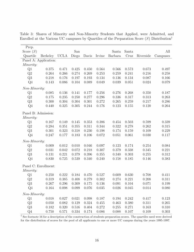
Table 3: Shares of Minority and Non-Minority Students that Applied, were Admitted, andEnrolled at the Various UC campuses by Quartiles of the Preparation Score (S) Distribution†

Prep.Score (S) San Santa Santa AllQuartile Berkeley UCLA Diego Davis Irvine Barbara Cruz Riverside CampusesPanel A: Application:Minority:

Q1 0.375 0.471 0.425 0.450 0.564 0.566 0.573 0.673 0.497Q2 0.264 0.266 0.274 0.269 0.253 0.259 0.241 0.216 0.258Q3 0.218 0.176 0.197 0.193 0.134 0.136 0.134 0.087 0.166Q4 0.143 0.086 0.104 0.089 0.049 0.039 0.051 0.024 0.079

Non-Minority:Q1 0.085 0.136 0.141 0.177 0.256 0.276 0.268 0.350 0.187Q2 0.175 0.235 0.250 0.277 0.296 0.336 0.317 0.313 0.263Q3 0.300 0.304 0.304 0.301 0.272 0.265 0.259 0.217 0.286Q4 0.440 0.325 0.305 0.244 0.176 0.123 0.155 0.120 0.264

Panel B: Admission:Minority:

Q1 0.167 0.149 0.145 0.353 0.386 0.454 0.503 0.599 0.339Q2 0.284 0.351 0.355 0.311 0.344 0.322 0.278 0.262 0.315Q3 0.301 0.323 0.318 0.230 0.198 0.174 0.159 0.109 0.229Q4 0.247 0.177 0.183 0.106 0.072 0.051 0.061 0.030 0.117

Non-Minority:Q1 0.009 0.012 0.010 0.046 0.097 0.123 0.174 0.254 0.084Q2 0.031 0.042 0.072 0.218 0.307 0.379 0.338 0.345 0.221Q3 0.131 0.221 0.379 0.396 0.355 0.340 0.303 0.255 0.312Q4 0.830 0.725 0.539 0.340 0.240 0.158 0.185 0.146 0.383

Panel C: Enrollment:Minority:

Q1 0.250 0.222 0.184 0.470 0.527 0.609 0.630 0.708 0.411Q2 0.319 0.385 0.408 0.279 0.302 0.274 0.221 0.208 0.311Q3 0.267 0.296 0.309 0.175 0.136 0.091 0.104 0.071 0.199Q4 0.164 0.098 0.099 0.076 0.035 0.026 0.045 0.014 0.080

Non-Minority:Q1 0.018 0.027 0.021 0.098 0.187 0.194 0.242 0.417 0.123Q2 0.050 0.082 0.129 0.324 0.455 0.463 0.380 0.311 0.265Q3 0.182 0.320 0.516 0.404 0.272 0.255 0.271 0.163 0.310Q4 0.750 0.571 0.334 0.174 0.086 0.088 0.107 0.109 0.303

† See footnote 16 for a description of the construction of students preparation scores. The quartiles used were derivedfor the distribution of scores for the pool of all applicants to one or more UC campus during the years 1995-1997.

16

students, with the first (second) set of columns showing results for 4-year (5-year) graduation

rates.

Considering first minority five-year graduation rates, those in the bottom two quartiles of the

preparation distribution at the top-2 campuses see significantly lower probabilities of graduating

in the sciences conditional on beginning in the sciences than those at the bottom-3. This result

holds even though students at UC Berkeley and UCLA with S scores in the bottom quartile

were presumably stronger in other dimensions, e.g., parental education, income, etc., than those

in the bottom quartile at the less selective institutions. Moving to the highest quartile, however,

shows virtually no difference in science persistence rates across the top-2 and bottom-3 campuses.

Further, results from the third quartile indicate significantly higher graduation probabilities in

the non-sciences among those attending the more selective campuses. Looking at non-minorities

also shows the top schools being a relatively better match for the top students. Students in the

top two quartiles have higher probabilities of persisting in the sciences, and significant positive

effects appear in the second quartile for graduating in the non-sciences. As a whole, these results

suggest the possibility that (i) less-prepared students may have higher graduation probabilities

at less-selective schools and (ii) this is especially true in the sciences.

The patterns of persistence in science majors and probabilities of graduating in any field are

even more striking if we instead examine 4-year graduation rates. Regardless of minority status,

no student in the bottom quartile at either UC Berkeley or UCLA finished a science degree in

four years conditional on beginning in the sciences. Both minorities and non-minorities in the

bottom three quartiles have significantly lower 4-year science persistence rates at the top-2

schools, and in all quartiles those who begin in a science major have significantly lower 4-

year graduation rates at the top-2 schools. For those who begin in the non-sciences in the

bottom two quartiles, significantly lower 4-year graduation rates are also found at the top-2

schools. However, no significant differences are present for initial non-science majors in the

top two quartiles for 4-year graduation rates, again suggesting that preparation is particularly

important in the sciences at the top schools.

17

Table 4: Comparison of Unadjusted 4- and 5-Year Graduation Rates (%) of Minority & Non-Minority Students for different Majors at Top 2 Ranked UC Campuses with the 3 LowestRanked, by S Quartile and Initial Major

4-year Graduation Rate 5-year Graduation RatePrep Ave. at Ave. at Ave. at Ave. atScore (S) Initial Final Top 2 Bottom 3 Top 2 Bottom 3Quartile Major Major Campuses Campuses Diff. Campuses Campuses DiffMinority:Q1 Science Science 0.0 5.1 -5.1∗∗ 9.3 13.8 -4.4∗

Science Any 7.0 17.7 -10.7∗∗ 43.9 49.1 -5.2Non-Science Any 17.3 32.7 -15.4∗∗ 59.0 58.7 0.3

Q2 Science Science 3.7 14.7 -11.0∗∗ 17.5 26.4 -8.9∗∗

Science Any 12.1 26.4 -14.3∗∗ 59.3 57.6 1.7Non-Science Any 28.6 42.7 -14.1∗∗ 67.0 67.2 -0.2

Q3 Science Science 8.3 18.7 -10.4∗∗ 28.9 36.2 -7.3Science Any 16.6 40.2 -23.6∗∗ 63.5 69.2 -5.7Non-Science Any 39.9 44.6 -4.8 76.8 68.6 8.2∗∗

Q4 Science Science 20.6 42.6 -22.0∗∗ 52.1 52.4 -0.3Science Any 35.7 63.9 -28.1∗∗ 78.3 78.6 -0.3Non-Science Any 52.0 62.5 -10.4 83.9 84.8 -1.0

Non-Minority:Q1 Science Science 0.0 8.6 -8.6∗∗ 17.5 21.0 -3.5

Science Any 0.0 24.0 -24.0∗∗ 50.0 54.2 -4.2Non-Science Any 20.1 39.0 -18.9∗∗ 58.5 63.9 -5.4∗

Q2 Science Science 9.1 14.6 -5.5∗ 28.7 28.5 0.2Science Any 18.8 32.0 -13.2∗∗ 67.0 61.3 5.8∗

Non-Science Any 37.6 46.9 -9.2∗∗ 78.8 72.1 6.7∗∗

Q3 Science Science 17.6 23.4 -5.8∗∗ 45.1 39.6 5.5∗∗

Science Any 31.5 43.0 -11.5∗∗ 78.1 70.2 8.0∗∗

Non-Science Any 49.7 49.6 0.0 83.5 74.6 9.0∗∗

Q4 Science Science 30.8 32.7 -1.9 58.1 46.6 11.4∗∗

Science Any 46.3 57.6 -11.3∗∗ 86.1 79.6 6.5∗∗

Non-Science Any 61.9 60.8 1.2 88.9 80.1 8.8∗∗

* and ** indicate significance at 10 and 5 level, respectively.

18

3 Modeling Student Persistence in College Majors and

Graduation

The descriptive statistics in Section 2.2 suggest that the match between students’ academic

preparation scores and the ranking of the UC campus may be important, particularly in the

sciences. We now propose a model that is flexible enough to capture these matching effects. We

model a student’s decision regarding whether to graduate from college and, if they do, their final

choice of major. In particular, student i attending college k can choose to major and graduate in

a science field, m, or in a non-science field, h, or choose to not graduate, n. Denote the student’s

decision by dik, dik ∈ {m,h, n}. In what follows, the student’s college, k, is taken as given. But,

as noted above, ignoring the choice process governing which campus a student selected may

give rise to selection bias in estimating the determinants of their choice of a major to the extent

that admission decisions are based on observed and unobserved student characteristics that also

may influence their choice of majors and likelihood of graduating from college. We discuss the

selection problem in more detail in section 3.2.

We assume that the utility student i derives from graduating with a major in j from college

k depends on three components: (i) the net returns she expects to receive from graduating with

this major from this college; (ii) the costs of switching one’s major, if the student decides to

change from the one with which she started college; and (iii) other factors which we treat as

idiosyncratic and stochastic. The net returns from majoring in field j at college k, Rijk, is just the

difference between the expected present value of future benefits, bijk, of having this major/college

combination, less the costs associated with completing it, cijk, i.e., Rijk = bijk − cijk.25 In

particular, the benefits would include the expected stream of labor market earnings that would

accrue to someone with this major-college combination (e.g., an engineering degree from UC

Berkeley), where these earnings would be expected to vary with a student’s ability and the

quality of training provided by the college.

The costs of completing a degree in field j at k depend on the effort a student would need

to exert to complete the curriculum in this major at this college, where this effort is likely to

25For a similar approach to modeling the interaction between colleges and majors in determining collegegraduations in particular majors, see Arcidiacono (2004).

19

vary with i’s academic preparation, the quality of the college and its students. With respect to

switching costs, each student arrives on campus with an initial major, jint (as with the college

she attends, her initial, or intended, major, jint, is taken as given). The student may remain in

and graduate with her initial major or may decide to switch to and graduate with a different

major in which case the switching cost, Cijk, is paid. Finally, we allow for an idiosyncratic taste

factor, εijk. It follows that the payoff function for graduating with major j at college k is given

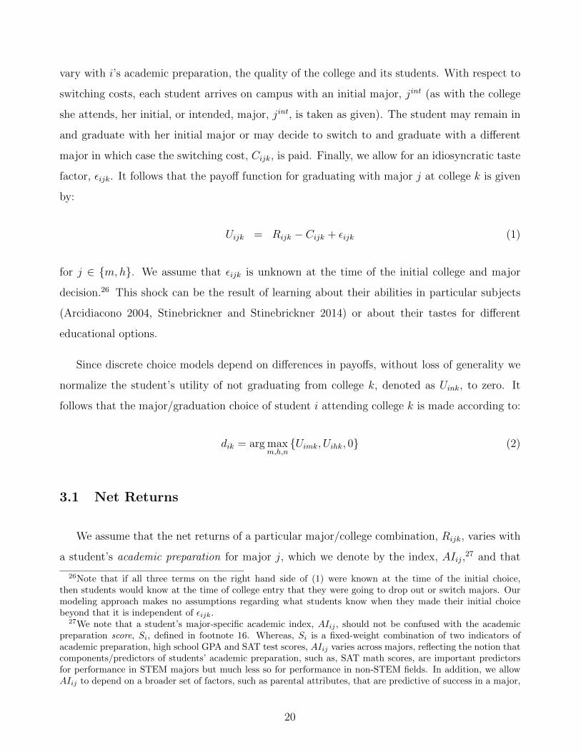
by:

Uijk = Rijk − Cijk + εijk (1)

for j ∈ {m,h}. We assume that εijk is unknown at the time of the initial college and major

decision.26 This shock can be the result of learning about their abilities in particular subjects

(Arcidiacono 2004, Stinebrickner and Stinebrickner 2014) or about their tastes for different

educational options.

Since discrete choice models depend on differences in payoffs, without loss of generality we

normalize the student’s utility of not graduating from college k, denoted as Uink, to zero. It

follows that the major/graduation choice of student i attending college k is made according to:

dik = arg maxm,h,n

{Uimk, Uihk, 0} (2)

3.1 Net Returns

We assume that the net returns of a particular major/college combination, Rijk, varies with

a student’s academic preparation for major j, which we denote by the index, AIij,27 and that

26Note that if all three terms on the right hand side of (1) were known at the time of the initial choice,then students would know at the time of college entry that they were going to drop out or switch majors. Ourmodeling approach makes no assumptions regarding what students know when they made their initial choicebeyond that it is independent of εijk.

27We note that a student’s major-specific academic index, AIij , should not be confused with the academicpreparation score, Si, defined in footnote 16. Whereas, Si is a fixed-weight combination of two indicators ofacademic preparation, high school GPA and SAT test scores, AIij varies across majors, reflecting the notion thatcomponents/predictors of students’ academic preparation, such as, SAT math scores, are important predictorsfor performance in STEM majors but much less so for performance in non-STEM fields. In addition, we allowAIij to depend on a broader set of factors, such as parental attributes, that are predictive of success in a major,

20

these net returns to AIij may differ across campuses. In particular, we assume that Rijk is

characterized by the linear function:

Rijk = φ1jk + φ2jkAIij (3)

The specification in (3) allows college-major combinations to differ in their net returns to aca-

demic preparation with higher net returns associated with higher values of φ2jk. As noted

above, such differences in φ2jk may result from colleges gearing their curriculum in a particular

major to students from a particular academic background which, in turn, produce differences in

subsequent labor market earnings. Degrees in various majors from different colleges also may

produce differing net returns that do not depend on a student’s academic preparation which

is reflected in differing values of φ1jk. For example, the curriculum in a particular major and

the course requirements that all students have to meet may vary across colleges, resulting in

colleges imposing differing effort and time costs to completing the major.

We are interested in how differences in college quality, or selectivity, affect major-specific

graduation probabilities for students of differing academic preparation. To see how the specifi-

cation of the net returns functions in (3) capture such differences, suppose that College A is an

elite, selective college (e.g., UC Berkeley or UCLA), while College B is a less selective one (e.g.,

UC Santa Cruz or UC Riverside). Three cases are illustrated in Figure 3. One possibility is

that highly selective colleges (A) have an absolute advantage relative to less selective ones (B)

in the net returns students from any level of academic preparation would receive and that such

advantage is true for all majors. This case is illustrated Figure 3(a), where the absolute advan-

tage holds for all majors. Alternatively, selective colleges may not generate higher net returns

for students with all levels of academic preparation in all fields. For example, selective colleges

may have an absolute advantage in moving all types of students through its science curriculum,

whereas less selective colleges (B) may have an absolute advantage in training students in the

humanities. This case is characterized by Figures 3(a) and 3(b), respectively, in which elite

colleges (A) have absolute advantage in getting students through major j, while less selective

colleges (B) have an absolute advantage in graduating all students from major j′. This second

whereas the score, Si, depends only on GPA and SAT tests scores.

21

Figure 3: Differences in Net Returns to Student Academic Preparation (AI) by Major at Se-lective (A) and Non-Selective (B) Colleges

Acad. Prep. (AIj)

College A

College B

Net Returns to

AIj for major j at college k

(Rjk)

(a) Net Returns to AIj of graduating in major j fromCollege A is greater than from B for all AIj .

Acad. Prep. (AIj′)

College B

College A

Net Returns to

AIj′ for major j′ at college k

(Rj′k)

(b) Net Returns to AIj′ of graduating in major j′ fromCollege B is greater than from A for all AIj′ .

College A

College B

Net Returns to

AIj for major j at college k

(Rjk)

Acad. Prep. (AIj)

(c) Net Returns to AIj of graduating in major j fromCollege A is greater than B for better prepared students,but greater from B than A for less prepared ones.

case might arise if colleges develop faculties and facilities to educate students in some majors,

but not others, such as “technology institutes” (e.g., Caltech, Georgia Tech) which focus their

curriculum primarily on science and technology fields.

But some colleges may produce higher net returns in some major j for less-prepared stu-

dents, while other colleges produce higher net returns for better-prepared students. This case is

illustrated in Figure 3(c). At first glance, this differences-in-relative-advantage between highly

selective and less selective colleges may account for the differential success UC Berkeley and

22

UCLA had in graduating minorities versus non-minorities with STEM majors compared to

lesser-ranked UC campuses, like UC Santa Cruz and UC Riverside. Below, we examine the

empirical validity of this latter explanation, after explicitly accounting for differences in student

preparation.

3.2 Academic Preparation for Majors

We now specify how the student’s major-specific academic preparation index, AIij, is con-

structed. We assume that the various abilities and factors that go into determining a student’s

preparation for a particular major can be characterized by a set of characteristics Xi. These

characteristics are then rewarded in majors differently. For example, math skills may be re-

warded more in the sciences while verbal scores may be more rewarded outside of the sciences.

It follows that the academic preparation index for major j ∈ {m,h}, AIij, is then given by:

AIij = Xiβj (4)

where subscripting β by j allows the weights on the various measures of preparation to vary by

major.

Our estimation problem is analogous to that in the literature concerning the effects of college

quality on graduation and later-life outcomes. In particular, whether a student remains in a

major and graduates from a particular college is the result of student decisions that are influenced

by the quality of the campus – in our case the campus-specific net returns to graduating with

a particular major and the costs of switching a major – and by observed and unobserved

dimensions of her academic preparation. The observed measures of academic preparation in Xi

includes high school GPA, SAT math and verbal scores, as well as family background measures

such as parental income and parental education. We also include indicator variables for minority

and Asian as race and ethnicity are correlated with factors such as high school quality, even

after controlling for parental education and income.28

To account for the selection effects based on unobservables, we employ the approach used

28See U.S. Department of Education (2000).

23

by Dale and Krueger (2002). In particular, we add to our controls dummy variables for whether

a student applied to each of the eight UC campuses, dummy variables for whether they were

accepted to each of these UC campuses, and some interactions of these variables.29 Because

racial preferences affect admissions and application probabilities, we also interact each of these

variables with minority status. This sort of approach requires that students not always attend

the most highly ranked for which they were admitted. In Appendix Table A-5, we show that

there is a sufficient number of cases where individuals are admitted to pairs of schools and choose

to attend the lower ranked of the pair, regardless of which school pairing we are considering.

This approach is not without critics,30 as the reasons why someone may choose to apply to a

top school, be admitted, and then attend a lower-ranked school are not obvious and may be

correlated with unobserved ability. Hence, in Section 4.3 we explore how our results are affected

by using different combinations of Dale and Krueger controls as well as not including them at

all.

3.3 Costs of Switching Majors

Finally, we specify the costs of switching majors, Cijk. We allow these costs depend on a

student’s initial major j and academic preparation index for that major, AIij, as well as allowing

separate effects for family background, Bi, as measured by parental income and education.

Further, these effects are allowed to vary by campus, α3k, with the specification of Cijk given

by:

Cijk =

α0j + α1jAIij + α2Bi + α3k, if jint 6= j,

0, if jint = j.

(5)

29The additional interactions are: i) whether the individual applied to any of the top three UC campuses, butwas rejected by one of the middle three UC campuses; ii) whether the individual applied to any of the top threeUC campuses, but was rejected by one of the bottom two UC campuses; iii) whether the individual appliedto any middle three UC campuses, but was rejected by one of the bottom two UC campuses; iv) whether theindividual was admitted to one of the top three UC campuses, but was rejected by one of the middle three UCcampuses; and v) whether the individuals was admitted to one of the top three schools and applied to one ofthe bottom two schools.

30See, for example, Hoxby (2009) page 115.

24

3.4 Estimation

We specify the error structure for the choice-specific utilities to have a nested logit form,

allowing the errors to be correlated among the two graduation options, i.e., graduating with a

science major (m) and graduating with a non-science major (h). In this way we account for

shocks after the initial choice of college and major that may influence the value of a student

continuing their education, such as a shock to one’s finances or personal issues. Given our

assumption regarding the error distribution, the probability of choosing to graduate from school

k with major j ∈ {m,h}, conditional on X and B (but not ε), is given by:

pijk(θ) =

(∑j′ exp

(uij′kρ

))ρ−1exp

(uijkρ

)(∑

j′ exp(uij′kρ

))ρ+ 1

, (6)

where θ ≡ {α, β, φ, ρ} is the full set of parameters to be estimated and uijk ≡ Uijk − εijk.31 The

probability of choosing not to graduate from k is then given by:32

pi0k(θ) =1(∑

j′ exp(uij′kρ

))ρ+ 1

, (7)

We estimate separate nested logit models for 4- and 5-year graduation outcomes.

Note that since βj is major-specific, we must normalize one of the φ2jk’s for each major.

We do so by setting the return on both the science and non-science academic index at UC

Berkeley to one. The estimated βj’s then give the returns to the various components of the

academic indexes at UC Berkeley in major j. In order to make our results easier to interpret,

the remaining φ2jk parameters are estimated relative to UC Berkeley. In particular, we estimate

φ∗2jk for the other campuses where φ∗2jk = φ2jk − 1. Similarly, we estimate the intercept terms

for the other campuses relative to UC Berkeley, estimating φ∗1jk where φ∗1jk = φ1jk − φ1jBERK .

31uijk is formed by substituting the expressions in (3) for Rijk, in (5) for Cijk, and in (4) for AIijk into (1).32Recall that we normalize the utility for not graduating to zero, i.e., ui0k = 0.

25

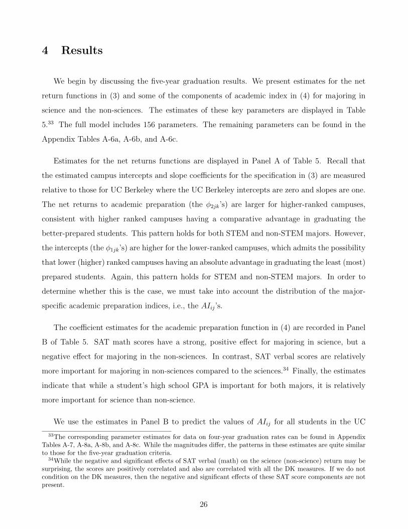
4 Results

We begin by discussing the five-year graduation results. We present estimates for the net

return functions in (3) and some of the components of academic index in (4) for majoring in

science and the non-sciences. The estimates of these key parameters are displayed in Table

5.33 The full model includes 156 parameters. The remaining parameters can be found in the

Appendix Tables A-6a, A-6b, and A-6c.

Estimates for the net returns functions are displayed in Panel A of Table 5. Recall that

the estimated campus intercepts and slope coefficients for the specification in (3) are measured

relative to those for UC Berkeley where the UC Berkeley intercepts are zero and slopes are one.

The net returns to academic preparation (the φ2jk’s) are larger for higher-ranked campuses,

consistent with higher ranked campuses having a comparative advantage in graduating the

better-prepared students. This pattern holds for both STEM and non-STEM majors. However,

the intercepts (the φ1jk’s) are higher for the lower-ranked campuses, which admits the possibility

that lower (higher) ranked campuses having an absolute advantage in graduating the least (most)

prepared students. Again, this pattern holds for STEM and non-STEM majors. In order to

determine whether this is the case, we must take into account the distribution of the major-

specific academic preparation indices, i.e., the AIij’s.

The coefficient estimates for the academic preparation function in (4) are recorded in Panel

B of Table 5. SAT math scores have a strong, positive effect for majoring in science, but a

negative effect for majoring in the non-sciences. In contrast, SAT verbal scores are relatively

more important for majoring in non-sciences compared to the sciences.34 Finally, the estimates

indicate that while a student’s high school GPA is important for both majors, it is relatively

more important for science than non-science.

We use the estimates in Panel B to predict the values of AIij for all students in the UC

33The corresponding parameter estimates for data on four-year graduation rates can be found in AppendixTables A-7, A-8a, A-8b, and A-8c. While the magnitudes differ, the patterns in these estimates are quite similarto those for the five-year graduation criteria.

34While the negative and significant effects of SAT verbal (math) on the science (non-science) return may besurprising, the scores are positively correlated and also are correlated with all the DK measures. If we do notcondition on the DK measures, then the negative and significant effects of these SAT score components are notpresent.

26

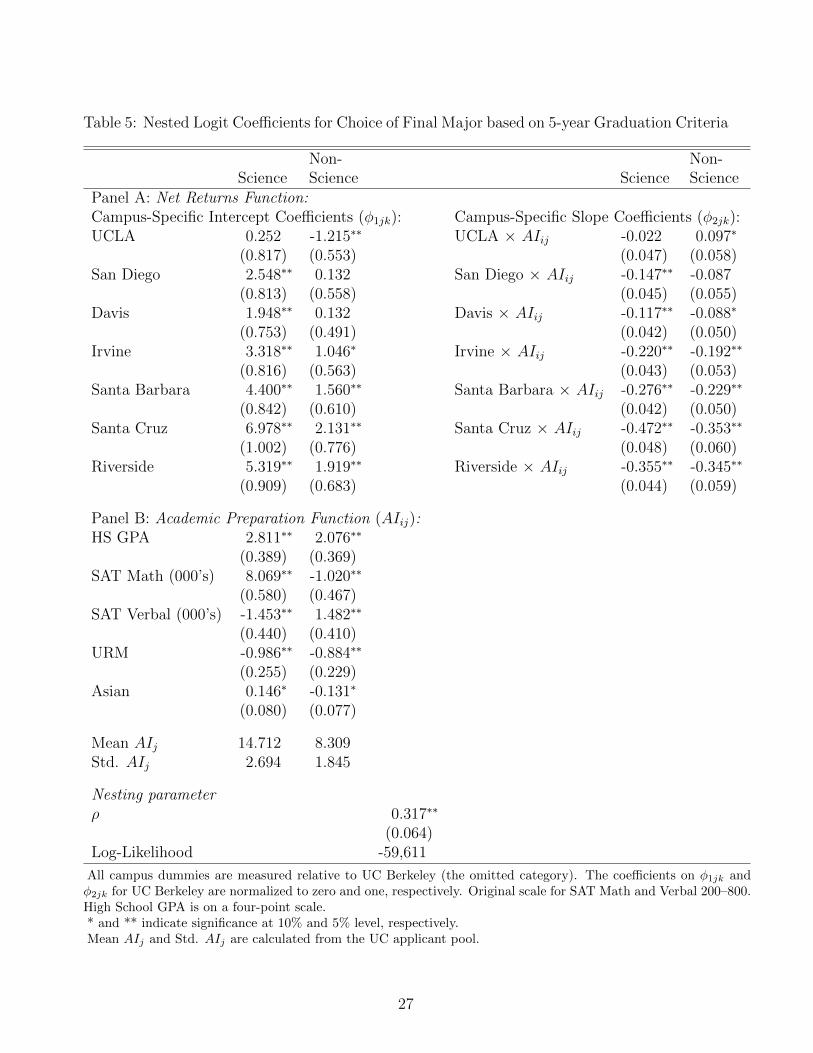
Table 5: Nested Logit Coefficients for Choice of Final Major based on 5-year Graduation Criteria

Non- Non-Science Science Science Science

Panel A: Net Returns Function:Campus-Specific Intercept Coefficients (φ1jk): Campus-Specific Slope Coefficients (φ2jk):UCLA 0.252 -1.215∗∗ UCLA × AIij -0.022 0.097∗

(0.817) (0.553) (0.047) (0.058)San Diego 2.548∗∗ 0.132 San Diego × AIij -0.147∗∗ -0.087

(0.813) (0.558) (0.045) (0.055)Davis 1.948∗∗ 0.132 Davis × AIij -0.117∗∗ -0.088∗

(0.753) (0.491) (0.042) (0.050)Irvine 3.318∗∗ 1.046∗ Irvine × AIij -0.220∗∗ -0.192∗∗

(0.816) (0.563) (0.043) (0.053)Santa Barbara 4.400∗∗ 1.560∗∗ Santa Barbara × AIij -0.276∗∗ -0.229∗∗

(0.842) (0.610) (0.042) (0.050)Santa Cruz 6.978∗∗ 2.131∗∗ Santa Cruz × AIij -0.472∗∗ -0.353∗∗

(1.002) (0.776) (0.048) (0.060)Riverside 5.319∗∗ 1.919∗∗ Riverside × AIij -0.355∗∗ -0.345∗∗

(0.909) (0.683) (0.044) (0.059)

Panel B: Academic Preparation Function (AIij):HS GPA 2.811∗∗ 2.076∗∗

(0.389) (0.369)SAT Math (000’s) 8.069∗∗ -1.020∗∗

(0.580) (0.467)SAT Verbal (000’s) -1.453∗∗ 1.482∗∗

(0.440) (0.410)URM -0.986∗∗ -0.884∗∗

(0.255) (0.229)Asian 0.146∗ -0.131∗

(0.080) (0.077)

Mean AIj 14.712 8.309Std. AIj 2.694 1.845

Nesting parameterρ 0.317∗∗

(0.064)Log-Likelihood -59,611

All campus dummies are measured relative to UC Berkeley (the omitted category). The coefficients on φ1jk andφ2jk for UC Berkeley are normalized to zero and one, respectively. Original scale for SAT Math and Verbal 200–800.High School GPA is on a four-point scale.* and ** indicate significance at 10% and 5% level, respectively.Mean AIj and Std. AIj are calculated from the UC applicant pool.

27

applicant pool who applied to a UC campus in the sciences (j = m) or non-sciences (j = h).

The mean and standard deviations for these two distributions are displayed immediately below

Panel B of Table 5. These distributions differ across the two majors. Such differences, especially

with respect to the variances, complicate comparisons of the gradients of net returns with respect

to student academic preparation across majors. To avoid this problem, we use the standardized

version of AIij for each major, i.e., AI∗ij ≡(AIij−AIj)sd(AIj)

, where AIj is the mean of AIij taken over

the entire UC applicant pool who declared their initial major in the sciences (j = m) and the

non-sciences (j = h), respectively. It follows that the gradient of Rjk with respect to AI∗ij is

given by φ2jk · sd(AIij). Thus, while the φ2jks are comparable in magnitude across majors, the

gradients with respect to AI∗ij will not be.

Figure 4 plots the net returns to the two majors across the AI∗im distribution at three cam-

puses: UC Berkeley, UC Santa Cruz and UC Riverside. In particular, Figure 4(a) plots the

net returns in the sciences based on graduating in 5 years, while Figure 4(b) plots the corre-

sponding returns for non-science majors. While it appears that UC Berkeley has an absolute

advantage over the two lower-ranked campuses in net returns of non-science majors in terms of

5-year graduation, at least over a 2-standard deviation range of AI∗, the same is not the case for

science majors. Rather, while UC Berkeley has higher net returns in the sciences for students

with above average AI∗s, both UC Santa Cruz and UC Riverside turn out to have higher net

returns for students with lower-than-average AI∗s. As a result, the matching of students to

campuses by academic preparation is much more important in the sciences than for non-science

fields.

We plot these same net returns to graduating in 4 years for initially majoring in science and

non-science, respectively, in Figures 4(c) and 4(d). The matching of students with interests in

the sciences to campuses is even more important for on-time graduation based on the estimated

net returns associated with graduation in 4 years. As shown in Figure 4(c), our estimates imply

that students with AI∗s at or below 1 standard deviation above the mean have higher net

returns to graduating in 4 years in the sciences at UC Santa Cruz or UC Riverside than they

would have at UC Berkeley. And, our estimated net returns for graduating in 4 years in the

non-sciences are no longer higher at UC Berkeley relative to the two lower-ranked campuses,

28

with the crossing point at about one standard deviation above the mean of the applicant pool.

The distributions of net returns to graduation at higher- versus lower-ranked UC campuses

illustrated in Figure 4 also suggest that there are potential gains to graduation rates of minorities

in the sciences from re-allocating students across the UC campuses by their academic prepara-

tion. To see this, consider the location of the average minority student at UC Berkeley initially

declared in the sciences. Based on the estimates for the academic preparation function in (4),

this student would have an AI∗ score of -0.04, barely below the mean score in the applicant

pool of AI∗m = 0, indicating that this student would have a higher net return at either Santa

Cruz or UC Riverside.35 In contrast, the average non-minority student at UC Berkeley that

initially declared in the sciences has an AI∗im of 1.30, above the overall mean and in the range

where UC Berkeley’s net returns exceed those of the other two schools. In the next section, we

examine how re-allocating minority and non-minority students in the sciences from top-ranked

to lower-ranked UC campuses would affect graduation rates in the sciences.

4.1 Potential Gains from Re-Allocating Students to CounterfactualCampuses

In this section we use our estimates of net returns to forecast how graduation outcomes

would change if students at the top two UC campuses (UC Berkeley and UCLA) had instead

attended one of the bottom two campuses (UC Santa Cruz and UC Riverside).36 We focus

on changes in the probability of: (i) graduating in the sciences, conditional on beginning in

the sciences; (ii) graduating in any major, conditional on beginning in the sciences; and (iii)

graduating with any major, conditional on beginning in the non-sciences.

Table 6 presents the results for minority students. The first set of rows gives the average

across all minority students who attended UC Berkeley (first set of columns) or UCLA (second

set of columns) while the next set breaks out the effects by quartile of the preparation score (S).

Our model predicts average gains of 4.3 and 7.2 percentage points for persisting in the sciences,

35The advantage of UC Santa Cruz or UC Riverside over UC Berkeley for the average minority student fromUC Berkeley is even stronger based on 4-year graduation rates.

36In the appendix we show the share of minority or non-minority students who would have higher graduationprobabilities at each possible counterfactual campus, both in the sciences and overall. See Tables A-9 and A-10.

29

Figure 4: Differences in Net Returns to Students’ Standardized Academic Preparation Index(AI∗ij) by Major at Different UC Campuses

-4-2

02

4N

et R

etur

ns to

Aca

dem

ic P

repa

ratio

n in

Sci

ence

s

-1 0 1Academic Preparation (A) - Standard Deviation Units

Berkeley S. Cruz Riverside

(a) Net Returns to AI∗im of graduating in sciencesin 5 years from UC Berkeley, UC Santa Cruz, andUC Riverside.

-4-2

02

4N

et R

etur

ns to

Aca

dem

ic P

repa

ratio

n in

Non

-Sci

ence

s

-1 0 1Academic Preparation (A) - Standard Deviation Units

Berkeley S. Cruz Riverside

(b) Net Returns to AI∗ih of graduating in non-sciences in 5 years from UC Berkeley, UC SantaCruz, and UC Riverside.

-4-2

02

4N

et R

etur

ns to

Aca

dem

ic P

repa

ratio

n In

dex

in S

cien

ces

-1 0 1Academic Preparation (AI) - Standard Deviation Units

Berkeley S. Cruz Riverside

(c) Net Returns to AI∗im of graduating in sciencesin 4 years from UC Berkeley, UC Santa Cruz, andUC Riverside.

-4-2

02

4N

et R

etur

ns to

Aca

dem

ic P

repa

ratio

n In

dex

in N

on-S

cien

ces

-1 0 1Academic Preparation (AI) - Standard Deviation Units

Berkeley S. Cruz Riverside

(d) Net Returns to AI∗ih of graduating in non-sciences in 4 years from UC Berkeley, UC SantaCruz, and UC Riverside.

on a base of 27.5%, from moving from UC Berkeley to UC Santa Cruz and UC Riverside,

respectively. The overall gains from moving students in the sciences from UCLA to UC Santa

Cruz are relatively small (2.3%) and statistically insignificant, but moving minority students

from UCLA to UC Riverside produces an increase in science graduation rates of 4.7 percentage

points on a base of 27.0%. There are almost no significant gains in total graduation rates,

regardless of initial major. The one exception is moving students who are initially non-science

majors from UC Berkeley to UC Riverside, which lowers graduation rates for this group by 3.8

percentage points off a base of 69.9%.

30

Looking across quartiles of the academic preparation score (S) distribution, one finds that

the gains in graduation rates from moving students from top- to lower-ranked UC campuses vary

significantly by quartile, particularly for science graduation rates. As recorded in Table 6, UC

Berkeley students in the bottom quartile of the S distribution who begin in the sciences would

see their graduation probabilities in the sciences more than double had they attended either

UC Santa Cruz or UC Riverside, increasing their graduation rate by 11.8 and 9.8 percentage

points, respectively, on a base of 8%. At the second quartile, those moving from UC Berkeley

to UC Santa Cruz or UC Riverside would see graduation rate increases in the sciences of 8.9

and 10.0 percentage points, respectively, on a base of 18.1%. The gains are insignificant for

those students in the third and fourth quartile of the S distribution, with the sign flipping for

the fourth quartile at UC Santa Cruz.

Similar patterns are observed for moving students from UCLA to the two lowest-ranked

campuses, though the gains to moving these students to either UC Santa Cruz or UC Riverside

are not as large. Moving UCLA students in the bottom quartile who intended to major in the

sciences to UC Santa Cruz or UC Riverside would increase science graduation rates by the 8.2

and 6.5 percentage points, respectively, on a base of 11.9%, with significant gains in the second

quartile as well for both campuses. Those UCLA science students in the fourth quartile of the S

distribution, however, would see significantly lower graduation rates by moving to Santa Cruz,

dropping 5.6 percentage points off a base of 44.2%.

Differences across the quartiles of the academic preparation score, S, in the gains from mov-

ing minority students across campuses also are seen for overall graduation rates. Those in the

bottom quartile who begin in the sciences at UCLA see significantly higher overall graduation

probabilities of moving to UC Santa Cruz or UC Riverside, with increases of 8.1 and 6.5 per-

centage points, respectively. The effects are not as pronounced for those at UC Berkeley, with

only the increases at Santa Cruz significantly positive. For those in the bottom quartile being

in the non-sciences, no significant effects are found those who begin at UC Berkeley, but those

who begin at UCLA would see increases of 5.0 and 3.5 percentage points at UC Santa Cruz and

UC Riverside, with the latter only significant at the 10% level.

For students in the top quartiles of S, our results imply that moving minority students from

31

UC Berkeley or UCLA to lower ranked schools result in significant losses in total graduation

rates, particularly for those who begin in the non-sciences. Those in the top quartile who begin

in the non-sciences at UC Berkeley see graduation rate decreases of 5.8 and 6.2 percentage points

at UC Santa Cruz and UC Riverside, respectively, on a base of 81.4%. Similar graduation rate

decreases are seen from moving well-prepared minority students from UCLA to UC Santa Cruz

or UC Riverside.

Table 7 repeats the analysis in Table 6 for non-minority students.37 The overall patterns for

non-minority students are very different than those found for minorities. Moving non-minority

students to UC Santa Cruz who begin in the sciences at UC Berkeley or UCLA would result in

significant decreases in science graduation rates, while moving them to UC Riverside would have

no effect. And overall graduation rates – regardless of initial major – would fall significantly by

moving these students from the two top-ranked UC campuses to the two ranked at the bottom.

But, while the overall rates are very different across minority and non-minority students,

breaking the results out by quartiles shows similar within-quartile patterns for the two groups.

The difference is very few non-minorities at UC Berkeley or UCLA are in the bottom two

quartiles. Similar to minority students, non-minority students in the bottom quartile who begin

in the sciences at UC Berkeley see increased graduation probabilities of 9.8 percentage points

at both UC Santa Cruz and UC Riverside on a base of 16%. At UCLA, the increases are 5.5

and 6.1 percentage points, respectively, on a base of 18.4%.

Breaking out the results by quartile of the preparation score shows that the difference in the

overall effects for minorities and non-minorities are being driven by the combination of minority

students coming into the top UC campuses with significantly worse academic backgrounds,

coupled with the importance of the match between the college and the student. In particular,

the top-ranked campuses are comparatively better at graduating the most prepared students,

with the lower-ranked campuses having an absolute advantage in graduating students in the

32

Tab

le6:

Est

imat

edG

ains

(Los

ses)

in5-

Yea

rG

raduat

ions

for

Min

orit

ies

inM

ovin

gfr

omH

igher

toL

ower

Ran

ked

UC

Cam

puse

s,by

Quar

tile

sof

Aca

dem

icP

repar

atio

nSco

reD

istr

ibuti

onan

dIn

itia

lM

ajo

r(P

erce

nta

geP

oints

)

Pre

p.

Ber

kele

yG

ain

from

Gai

nfr

omU

CL

AG

ain

from

Gai

nfr

omSco

re(S

)In

itia

lF

inal

Bas

esw

itch

tosw

itch

toB

ase

swit

chto

swit

chto

Quar

tile

Majo

rM

ajo

rG

rad.

Rat

eSan

taC

ruz

Riv

ersi

de

Gra

d.

Rat

eSan

taC

ruz

Riv

ersi

de

Ove

rall

Sci

ence

Sci

ence

27.5

4.3∗∗

7.2∗∗

27.0

2.3

4.7∗∗

Sci

ence

Any

64.6

-1.6

-1.8

60.8

1.6

1.2

Non

-Sci

ence

Any

69.9

-2.7

-3.8∗∗

67.7

0.5

-0.6

Q1

Sci

ence

Sci

ence

8.0

11.8∗∗

9.8∗∗

11.9

8.2∗∗

6.5∗∗

Sci

ence

Any

47.4

4.5∗

2.8

45.0

8.1∗∗

6.5∗∗

Non

-Sci

ence

Any

59.8

0.3

-1.2

56.3

5.0∗∗

3.5

Q2

Sci

ence

Sci

ence

18.1

8.9∗∗

10∗∗

21.6

4.9∗∗

5.9∗∗

Sci

ence

Any

59.9

0.2

-0.6

57.5

3.0∗

2.2

Non

-Sci

ence

Any

69.6

-2.7

-3.9∗∗

67.3

0.6

-0.6

Q3

Sci

ence

Sci

ence

30.0

3.7

7.4∗∗

32.1

0.4

4.0∗

Sci

ence

Any

67.4

-2.5

-2.5

65.4

-0.4

-0.4

Non

-Sci

ence

Any

76.3

-4.6∗∗

-5.4∗∗

75.0

-2.3∗

-3.1∗

Q4

Sci

ence

Sci

ence

43.8

-3.5

3.0

44.2

-5.6∗∗

1.1

Sci

ence

Any

74.9

-5.3∗∗

-4.4∗∗

74.3

-4.1∗∗

-3.2∗

Non

-Sci

ence

Any

81.4

-5.8∗∗

-6.2∗∗

80.9

-4.3∗∗

-4.7∗∗

*an

d**

den

ote

that

the

chan

geis

stat

isti

call

ysi

gn

ifica

nt

at

10%

or

5%

leve

l,re

spec

tivel

y.

33

Tab

le7:

Est

imat

edG

ains

(Los

ses)

in5-

Yea

rG

raduat

ions

for

Non

-Min

orit

ies

inM

ovin

gfr

omH

igher

toL

ower

Ran

ked

UC

Cam

puse

s,by

Quar

tile

sof

Aca

dem

icP

repar

atio

nSco

reD

istr

ibuti

onan

dIn

itia

lM

ajo

r(P

erce

nta

geP

oints

)

Pre

p.

Ber

kele

yG

ain

from

Gai

nfr

omU

CL

AG

ain

from

Gai

nfr

omSco

re(S

)In

itia

lF

inal

Bas

esw

itch

tosw

itch

toB

ase

swit

chto

swit

chto

Quar

tile

Majo

rM

ajo

rG

rad.

Rat

eSan

taC

ruz

Riv

ersi

de

Gra

d.

Rat

eSan

taC

ruz

Riv

ersi

de

Ove

rall

Sci

ence

Sci

ence

56.4

-11.

9∗∗

-0.8

50.3

-9.2∗∗

0.6

Sci

ence

Any

84.7

-8.0∗∗

-6.3∗∗

81.4

-6.3∗∗

-4.9∗∗

Non

-Sci

ence

Any

86.9

-6.4∗∗

-6.4∗∗

84.8

-5.1∗∗

-5.3∗∗

Q1

Sci

ence

Sci

ence

16.0

9.8∗∗

9.8∗∗

18.4

5.5∗∗

6.1∗∗

Sci

ence

Any

55.5

2.1

1.0

57.0

3.2∗

2.3

Non

-Sci

ence

Any

70.6

-3.2∗

-4.3∗∗

67.1

0.5

-0.7

Q2

Sci

ence

Sci

ence

30.0

3.1

7.3∗∗

33.3

-0.8

3.7∗

Sci

ence

Any

69.8

-3.4∗∗

-3.3∗∗

68.5

-1.6

-1.4

Non

-Sci

ence

Any

77.2

-4.7∗∗

-5.5∗∗

75.2

-2.4

-3.2∗∗

Q3

Sci

ence

Sci

ence

49.0

-7.2∗∗

1.4

45.3

-6.7∗∗

1.6

Sci

ence

Any

80.0

-6.9∗∗

-5.6∗∗

78.2

-5.3∗∗

-4.3∗∗

Non

-Sci

ence

Any

84.3

-6.2∗∗

-6.4∗∗

84.2

-5.1∗∗

-5.4∗∗

Q4

Sci

ence

Sci

ence

58.9

-13.

4∗∗

-1.5

54.5

-11.

3∗∗

-0.2

Sci

ence

Any

86.3

-8.4∗∗

-6.5∗∗

84.3

-7.3∗∗

-5.6∗∗

Non

-Sci

ence

Any

89.3

-6.8∗∗

-6.5∗∗

88.5

-6.1∗∗

-6.0∗∗

*an

d**

den

ote

that

the

chan

geis

stat

isti

call

ysi

gn

ifica

nt

at

10%

or

5%

leve

l,re

spec

tivel

y.

34

sciences who are at the bottom of the preparation distribution.

4.2 Predicted Graduation Rates under Alternative Assignment Rules

The results in the preceding two sections suggest that matching of students to campuses

according to their academic preparation matters for graduation rates in the sciences. Moreover,

it appears that these gains in the sciences are greater for minorities than non-minorities. As

noted, the latter finding is driven by the differences in the way minority and non-minority stu-

dents were allocated across the UC campuses in a period where racial preferences were present.

Our model also allows us to examine how minority graduation rates would have changed under

other, i.e., counterfactual, rules of assigning this group to the UC campuses. For example, what

would have happened to minority graduation rates had minorities been allocated to universities

in the way non-minority students were? Similarly, we can examine how graduation rates for

non-minorities would be affected had they been assigned like minorities. Would their science

graduation rates fall or rise under this alternative assignment mechanism? To address these

questions, we use our estimates of students’ selection-adjusted graduation probabilities – the

pijk(θ)’s in (6) and (7) – along with probabilities of students’ being assigned to each of these

campuses as a function of their academic preparation indices – the AI ij’s – in order to assess the

magnitudes of the potential gain in minority graduation rates from this counterfactual allocation

of students across the UC campuses.

To proceed, we first estimate assignment rules allocating non-minority and minority stu-

dents, respectively, across the eight UC campuses for each of the two intended majors, using

multinomial logits. We assume that the probability of student i in race/ethnic group r (minority

or non-minority) being assigned to campus k is the following function of the student’s estimated

academic preparation indices, AI im and AI ih, for field of study j ∈ {m,h}:38

qijkr(πjkr) =exp

(π1jkr + π2jkrAI im + π3jkrAI ih

)∑

k exp(π1jkr + π2jkrAI im + π3jkrAI ih

) , (8)

37Using whites as a comparison group (as opposed to non-minorities as a whole) yielded similar patterns.38By using the estimated academic indices as our two regressors we implicitly control for unobserved ability

through the Dale and Krueger controls.

35

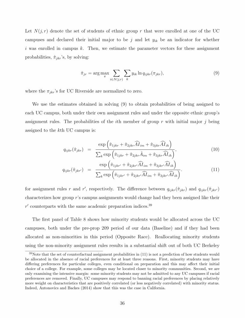
Let N(j, r) denote the set of students of ethnic group r that were enrolled at one of the UC

campuses and declared their initial major to be j and let yik be an indicator for whether

i was enrolled in campus k. Then, we estimate the parameter vectors for these assignment

probabilities, πjkr’s, by solving:

πjr = arg maxπ

∑i∈N(j,r)

∑k

yik ln qijkr(πjkr), (9)

where the πjkr’s for UC Riverside are normalized to zero.

We use the estimates obtained in solving (9) to obtain probabilities of being assigned to

each UC campus, both under their own assignment rules and under the opposite ethnic group’s

assignment rules. The probabilities of the ith member of group r with initial major j being

assigned to the kth UC campus is:

qijkr(πjkr) =exp

(π1jkr + π2jkrAI im + π3jkrAI ih

)∑

k exp(π1jkr + π2jkrAim + π3jkrAI ih

) , (10)

qijkr(πjkr′) =exp

(π1jkr′ + π2jkr′AI im + π3jkr′AI ih

)∑

k exp(π1jkr′ + π2jkr′AI im + π3jkr′AI ih

) . (11)

for assignment rules r and r′, respectively. The difference between qijkr(πjkr) and qijkr(πjkr′)

characterizes how group r’s campus assignments would change had they been assigned like their

r′ counterparts with the same academic preparation indices.39

The first panel of Table 8 shows how minority students would be allocated across the UC

campuses, both under the pre-prop 209 period of our data (Baseline) and if they had been

allocated as non-minorities in this period (Opposite Race). Reallocating minority students

using the non-minority assignment rules results in a substantial shift out of both UC Berkeley

39Note that the set of counterfactual assignment probabilities in (11) is not a prediction of how students wouldbe allocated in the absence of racial preferences for at least three reasons. First, minority students may havediffering preferences for particular colleges, even conditional on preparation and this may affect their initialchoice of a college. For example, some colleges may be located closer to minority communities. Second, we areonly examining the intensive margin: some minority students may not be admitted to any UC campuses if racialpreferences are removed. Finally, UC campuses may respond to banning racial preferences by placing relativelymore weight on characteristics that are positively correlated (or less negatively correlated) with minority status.Indeed, Antonovics and Backes (2014) show that this was the case in California.

36

and UCLA and into the four bottom-ranked UC campuses. The shifts are slightly different

depending on initial major, but the qualitative patterns are the same. The second panel shows

the same results for non-minority students under the baseline and if they were allocated across

the campuses in the same way that minorities had been (opposite race). Following the latter

assignment rule would move non-minority students out of the bottom four campuses and out of

UC Davis and into UC Berkeley and UCLA.

Finally, we use the estimated assignment probabilities to predict how graduation probabilities

in particular fields would change under different assignment rules. As in Tables 6 and 7, we

focus on changes in the probability of: (i) graduating in the sciences, conditional on beginning

in the sciences; (ii) graduating in any major, conditional on beginning in the sciences; and (iii)

graduating with any major, conditional on beginning in the non-sciences. In particular, these

predicted probabilities for group r, using the assignment rule of group r′, are given by:

Pr(g,m|m, r, r′) =

∑i

∑k I(i ∈ N(m, r))qijkr(πmkr′)pimk(θ)∑

i I(i ∈ N(m, r)), (12)

Pr(g|m, r, r′) =

∑i

∑k I(i ∈ N(m, r))qiskr(πmkr′)(pimk(θ) + pihk(θ))∑

i I(i ∈ N(m, r)), (13)

Pr(g|h, r, r′) =

∑i

∑k I(i ∈ N(h, r))qihkr(πhkr′)(pimk(θ) + pihk(θ))∑

i I(i ∈ N(h, r)), (14)

where I denotes the indicator function, g denotes the event of graduating from college, and

where the pijk(θ)’s are the predicted probabilities of student i graduating with major j from

campus k, using the estimates θ in place of θ in equation (6).

Table 9 displays the predictions of our model for how changes in campus assignment rules

would affect the graduation rates of minority and non-minority students. For both groups,

we first report graduation probabilities using their baseline assignment rules and then report

the change when the opposite group’s assignment rules are used. The top set of rows show

the overall effects on science graduation rates for those with an initial interest in the science,

overall graduation rates for those who are interested in the sciences, and overall graduation

rates for those intending not to major in a STEM field. Allocating minorities according the

non-minority assignment rules results in an average increase science persistence rates of 1.75

37

Tab

le8:

Shar

eof

Min

orit

yan

dN

on-M

inor

ity

Stu

den

tsU

nder

Diff

eren

tA

ssig

nm

ent

Rule

s(%

)

Init

ial

Ass

ignm

ent

San

San

taSan

taM

ajo

rR

ule

Ber

kele

yU

CL

AD

iego

Dav

isIr

vin

eB

arbar

aC

ruz

Riv

ersi

de

Min

orit

ySci

ence

Bas

elin

e13

.920

.611

.715

.312

.112

.15.

98.

6O

pp

osit

eR

ace

2.7

4.6

8.3

14.8

22.1

19.3

14.3

13.8

Non

-Sci

ence

Bas

elin

e19

.922

.66.

99.

97.

215

.78.

59.

3O

pp

osit

eR

ace

2.8

4.5

4.9

11.2

16.5

26.5

19.3

14.4

Non

-Min

orit

ySci

ence

Bas

elin

e16

.014

.816

.116

.814

.89.

95.

06.

6O

pp

osit

eR

ace

23.6

29.5

18.3

9.5

9.1

4.9

1.7

3.5

Non

-Sci

ence

Bas

elin

e13

.314

.611

.614

.412

.318

.010

.15.

7O

pp

osit

eR

ace

26.6

33.6

12.4

6.2

5.6

7.9

3.9

3.9

38

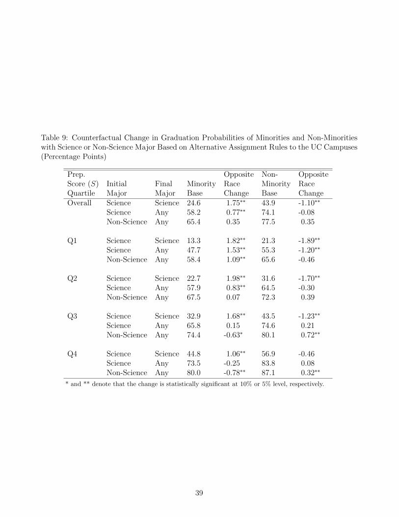
Table 9: Counterfactual Change in Graduation Probabilities of Minorities and Non-Minoritieswith Science or Non-Science Major Based on Alternative Assignment Rules to the UC Campuses(Percentage Points)

Prep. Opposite Non- OppositeScore (S) Initial Final Minority Race Minority RaceQuartile Major Major Base Change Base ChangeOverall Science Science 24.6 1.75∗∗ 43.9 -1.10∗∗

Science Any 58.2 0.77∗∗ 74.1 -0.08Non-Science Any 65.4 0.35 77.5 0.35

Q1 Science Science 13.3 1.82∗∗ 21.3 -1.89∗∗

Science Any 47.7 1.53∗∗ 55.3 -1.20∗∗

Non-Science Any 58.4 1.09∗∗ 65.6 -0.46

Q2 Science Science 22.7 1.98∗∗ 31.6 -1.70∗∗

Science Any 57.9 0.83∗∗ 64.5 -0.30Non-Science Any 67.5 0.07 72.3 0.39

Q3 Science Science 32.9 1.68∗∗ 43.5 -1.23∗∗

Science Any 65.8 0.15 74.6 0.21Non-Science Any 74.4 -0.63∗ 80.1 0.72∗∗

Q4 Science Science 44.8 1.06∗∗ 56.9 -0.46Science Any 73.5 -0.25 83.8 0.08Non-Science Any 80.0 -0.78∗∗ 87.1 0.32∗∗

* and ** denote that the change is statistically significant at 10% or 5% level, respectively.

39

percentage points, which is a little over a 7% increase on the base rate of 24.6%. Smaller, though

still statistically significant, graduation gains are predicted for overall graduation rates among

the initial science majors at 0.77 percentage points, with no significant changes in graduation

rates for minorities with initial non-science majors.

The next set of rows in Table 9 display the gains and losses in graduation rates by the

quartiles of the academic preparation score, S, used earlier in the paper. Predicted gains in

science persistence rates for minorities from being assigned according to the non-minority rules

are generally higher for those with lower levels of preparation. The bottom quartile also sees

higher overall gains in graduation rates as well. In contrast, minorities in the top two quartiles

who begin in a non-science majors see significant decreases in their graduation probabilities

using the alternative assignment rule.

As the last two columns of Table 9 indicate, non-minority students would experience lower

graduation rates in the sciences if they were assigned to UC campuses according to the as-

signment rules of minorities. Note that, quartile by quartile, the results of reallocating non-

minorities according to minority assignment rules would produce changes in graduation rates

that are almost always the same magnitude as what would occur for minorities by reassigning

them according to non-minority rules, but the changes go in the opposite direction. This is not

surprising since, as we have seen in Table 8, the non-minority rules better matched students to

schools in the sciences.

Note that these results ignore general equilibrium effects in how preparation translates into

outcomes at the different campuses. General equilibrium effects could arise from two potentially

conflicting sources: peer effects and endogenous grading standards. How peer effects would affect

our findings would depend on who is in the relevant peer group. On the one hand, if the peer

group was the whole student body, then reassigning minority students to lower ranked schools

may result in lowering the average preparation level at that school, which could in turn have

negative consequences for learning. The flip side of this is that lowering the average preparation

level of the student body may result in lowering grading standards which may result in higher

graduation probabilities. Further, if the relevant peers for minority students are primarily other

minority students, then we may be underestimating the gains from reallocation. In this case,

40

reassigning minority students to lower ranked schools results in average minority preparation

rising at all schools. Our results suggest lower ranked campuses would have produced higher

graduation rates for many minority students in the sciences who were at the higher ranked

campuses. This occurred despite these lower ranked campuses having a less-prepared student

body, suggesting that increasing the academic preparation of the minority student body at these

less selective schools may lead to even further improvements in graduation rates.40 We leave

estimation of general equilibrium effects to future work.

4.3 Robustness Checks

Until now, we have focused on one set of results using a particular specification for the

Dale and Krueger controls. We have estimated a number of other specifications with similar

qualitative patterns. Here we show how the last set of results – on how minority graduation

probabilities would change if they were allocated according the non-minority rules – varies with

alternative specifications of the graduation model. We consider four alternative models:

1. A specification where no Dale and Krueger controls are used. This will likely bias ourresults in favor of racial preferences due to selection on unobservables.

2. A specification where we interact all Dale and Krueger controls with whether or not oneof the parents was a college graduate.

3. A specification where we treat the initial major as the major listed on the application ofthe UC campus for which the individual eventually enrolled.

4. A specification where we allow for a campus-specific adjustment to the slopes and inter-cepts for minority students to see whether the production technology is different in somemanner for this group. This would be the case, for example, if campuses differed in howthey supported minority students.

Note that in each of the cases the estimates of academic preparation indices, AI ij, change as

well and we use these new estimates in our reassignments.

Results are presented in Table 10. With the exception of the case where no Dale and

Krueger controls are used, the results are quite similar across the different specifications. But,

40Improvements also would be seen for minorities who remain at the top schools as the average preparationlevels for minority students would rise here as well.

41

even absent the Dale and Krueger controls, the overall probability of graduating in the sciences

conditional on an initial science major is significantly higher for minority students with the

removal of racial preferences; a little over half the magnitude in our baseline specification.

While all the other specifications show significant graduation gains in the sciences across all

quartiles, absent the Dale and Krueger controls the effects are only significant for the bottom

two quartiles. This specification also produces significant negative effects on overall graduation

rates for initial non-science majors. Overall, the evidence is robust that reallocating minority

students to less selective colleges would increase science graduation rates.41

Table 10: Counterfactual Change in Graduation Probabilities of Minorities with Science orNon-Science Major Based on Non-Minority Assignment Rules to the UC Campuses (PercentagePoints)

Dale-No Krueger Campus

Prep. Dale- × Parent Altern. InterceptsScore (S) Initial Final Base Krueger College Major & SlopesQuartile Major Major Model Controls Educated Defn. × RaceOverall Science Science 1.75∗∗ 0.90∗∗ 1.67∗∗ 1.89∗∗ 1.82∗∗

Science Any 0.77∗∗ -0.47 0.77∗∗ 0.61∗ 1.04∗

Non-Science Any 0.35 -0.58∗ 0.39 0.40 0.56

Q1 Science Science 1.82∗∗ 1.29∗∗ 1.79∗∗ 1.95∗∗ 1.92∗∗

Science Any 1.53∗∗ 0.61∗∗ 1.55∗∗ 1.43∗∗ 2.07∗∗

Non-Science Any 1.09∗∗ 0.33 1.14∗∗ 1.20∗∗ 1.56∗∗

Q2 Science Science 1.98∗∗ 1.08∗∗ 1.89∗∗ 2.26∗∗ 2.08∗∗

Science Any 0.83∗∗ -0.62∗ 0.83∗∗ 0.68∗ 1.16∗

Non-Science Any 0.07 -1.04∗∗ 0.10 0.09 0.22

Q3 Science Science 1.68∗∗ 0.54 1.55∗∗ 1.79∗∗ 1.73∗∗

Science Any 0.15 -1.36∗∗ 0.14 -0.02 0.18Non-Science Any -0.63∗ -1.76∗∗ -0.63∗ -0.66∗∗ -0.80

Q4 Science Science 1.06∗∗ 0.02 0.94∗∗ 1.02∗∗ 1.02Science Any -0.25 -1.32∗∗ -0.26 -0.33 -0.46Non-Science Any -0.78∗∗ -1.60∗∗ -0.78∗∗ -0.86∗∗ -1.11∗∗

* and ** denote that the change is statistically significant at 10% or 5% level, respectively.

41Table A-11 presents the robustness checks for non-minorities, showing similar patterns to the last twocolumns of Table 9.

42

5 Why don’t less-prepared minorities go UC Riverside

and graduate in the sciences?

The size of the potential gains in graduation rates in the sciences of re-allocating less-prepared

minority students from higher- to lower-ranked campuses raises an obvious question: Why were

these gains not realized? A definitive answer to this question is beyond the scope of our data

and analysis. But, in this section, we explore some potential reasons why less-prepared students

who are interested in the sciences choose to attend colleges where success in the sciences is

unlikely.

We begin with the argument that the lack minorities graduating in the sciences at top-ranked

versus lower-ranked campuses simply reflects the self-interest of these students. For example,

perhaps it is the case that the returns to attending a top-ranked school are high regardless of

one’s major, with one’s major only mattering for earnings at lower-ranked campuses. In this

case, there would be a natural shift away from the sciences at top-ranked institutions relative to

their lesser-ranked counterparts. Our data does not allow us to directly address this possibility,

since we do not have information on expected or realized wages of the students in our data.

But, in an attempt to shed light on the potential importance of this explanation, we examine

the relationship between one’s major and the ranking of one’s college and wages using data from

the Baccalaureate and Beyond (B&B) study.

Individuals in the B&B received their BA/BS degree during the 1992-93 academic year.42

B&B respondents were interviewed in 1994, 1997 and 2003, respectively, were asked for their

major field of study as an undergraduate in the 1994 wave, and, in that and subsequent waves,

were asked about their employment and earnings. B&B respondents were asked whether they

were currently working and, if so, about their current earnings and hours of work. We use this

information to construct hourly wage rates for those who worked.43 We use the log of hourly

42The B&B sample was drawn from the 1992-93 National Postsecondary Student Aid Study (NPSAS:93), astudy of how undergraduate, graduate, and professional students and their families financed their postsecondaryeducation. Students in the NPSAS:93 completed a baseline interview in the 1992-93 school year which collecteddemographic and background characteristics about students and about their college. The B&B selected a samplefrom the NPSAS:93 that had earned a bachelor’s degree during the 1992-93 academic year. See Wine et al. (2005)for documentation of the sample and data collected in this study.

43We excluded those person-year observations that a calculated hourly wage rate greater than $500 and less

43

wages as the dependent variable in all of our regressions, using person-years of data only for those

years in which respondents reported to have worked. We classified B&B respondents as having

STEM or non-STEM majors, using the same classification system as that in the UCOP data.

Finally, to characterize the quality or ranking of the college/university from which each B&B

respondent graduated, we used the college’s average SAT scores of their entering class of 1990,

obtained from the U.S. News & World Report’s” 1991 Directory of Colleges and Universities.44

The results from a series of log wage regressions using the B&B data are presented in Table

11. The odd-numbered columns show unadjusted wage returns for different combinations of

college major and rankings of college, while the even-number columns provide the correspond-

ing estimates that adjust for test scores and background characteristics described in the table

footnote. In columns (1) and (2) of Table 11, we present estimates of the returns to graduating

with a STEM major. Consistent with the previous literature,45 we find sizable wage returns to

graduating with a STEM major, varying between 19% and 21%. Columns (3) and (4) contain

estimates of the returns to graduating from college by quartiles of the distribution of the av-

erage SAT score of colleges attended. Consistent with the previous literature,46 students that

graduate from more highly ranked colleges have, on average, higher wages. For example, stu-

dents that graduate from a college in the highest quartile of the average SAT score distribution

earned wages that were almost 14% higher than students who graduated from a college in the

bottom quartile, while graduates from a college in the second and third quartiles earned 3.76%

and 9.53% more, respectively, than those who graduated from a college in the bottom quartile.

In the final two columns of Table 11, we interact the STEM major and college ranking

quartile dummies. We use these coefficients to calculate the differences in average wage returns

between graduating with a non-STEM degree from a college ranking in a particular quartile

than the federal minimum wage rate for the particular year in question.44To determine the institution that each B&B respondent attended, we obtained a restricted-use version of the

B&B data that contained the Integrated Post-secondary Education Data System (IPEDS) IDs for the institutionfrom which each graduated. Using these IDs, we were able to link each college’s average SAT score. To formthe quartiles, we took the average SAT score of the school, weighted it by each college’s 1990 entering classenrollment, and took the quartile cut points from this weighted distribution. By this method of ranking colleges,UC Berkeley, UCLA, and UC San Diego were in the highest quartile, UC Davis, UC Irvine, UC Santa Barbara,and UC Santa Cruz were in the second highest, with UC Riverside in the third-highest.

45See Altonji, Blom, and Meghir (2012) for a review of the literature on returns to majors.46See Oreopoulos and Petronijevic for a review of the literature on returns to college quality.

44

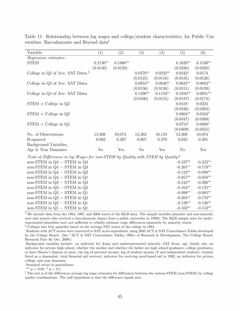
Table 11: Relationship between log wages and college/student characteristics, for Public Uni-versities: Baccalaureate and Beyond data†

Variable (1) (2) (3) (4) (5) (6)Regression estimates:STEM 0.2130∗∗ 0.1860∗∗ 0.1620∗∗ 0.1530∗∗

(0.0130) (0.0120) (0.0220) (0.0202)College in Q2 of Ave. SAT Distn.§ 0.0376∗∗ 0.0232∗∗ 0.0242∗ 0.0174

(0.0125) (0.0116) (0.0135) (0.0126)College in Q3 of Ave. SAT Distn. 0.0953∗∗ 0.0838∗∗ 0.0635∗∗ 0.0682∗∗

(0.0136) (0.0126) (0.0151) (0.0139)College in Q4 of Ave. SAT Distn. 0.1390∗∗ 0.1150∗∗ 0.1050∗∗ 0.0951∗∗

(0.0166) (0.0155) (0.0187) (0.0173)STEM × College in Q2 0.0418 0.0224

(0.0336) (0.0302)STEM × College in Q3 0.0804∗∗ 0.0524∗

(0.0347) (0.0309)STEM × College in Q4 0.0755∗ 0.0688∗

(0.0409) (0.0355)No. of Observations 13,308 10,074 13,362 10,110 13,308 10,074R-squared 0.002 0.387 0.007 0.378 0.025 0.391Background Variables,Age & Year Dummies No Yes No Yes No Yes

Tests of Differences in log Wages for non-STEM by Quality with STEM by Quality:‡

non-STEM in Q4 − STEM in Q4 -0.237∗∗ -0.222∗∗

non-STEM in Q4 − STEM in Q3 -0.201∗∗ -0.179∗∗

non-STEM in Q4 − STEM in Q2 -0.123∗∗ -0.098∗∗

non-STEM in Q4 − STEM in Q1 -0.057∗∗ -0.058∗∗

non-STEM in Q3 − STEM in Q3 -0.242∗∗ -0.206∗∗

non-STEM in Q3 − STEM in Q2 -0.164∗∗ -0.125∗∗

non-STEM in Q3 − STEM in Q1 -0.098∗∗ -0.085∗∗

non-STEM in Q2 − STEM in Q2 -0.204∗∗ -0.176∗∗

non-STEM in Q2 − STEM in Q1 -0.138∗∗ -0.136∗∗

non-STEM in Q1 − STEM in Q1 -0.162∗∗ -0.153∗∗

‡ We include data from the 1994, 1997, and 2003 waves of the B&B data. The sample includes minority and non-minoritymen and women who received a baccalaureate degree from a public university in 19993. The B&B sample sizes for under-represented minorities were not sufficient to reliably estimate wage differences separately by minority status.§ Colleges into four quartiles based on the average SAT scores of the college in 1994.Students with ACT scores were converted to SAT score-equivalents, using 2005 ACT & SAT Concordance Tables developed

by the College Board. (See ”ACT & SAT Concordance Tables, Office of Research & Development, The College Board,Research Note 40, Oct. 2009.)Background variables include: an indicator for Asian and underrepresented minority, SAT Score, age, family size, an

indicator for private high school, whether the mother and whether the father are high school graduates, college graduates,or have Master’s degrees or more, the log of parental income, log of student income (if and independent student), studentlisted as a dependent, total financial aid received, indicator for receiving need-based aid in 1992, an indicator for privatecollege, and year dummies.Standard errors in parentheses.** p < 0.05; * p < 0.1.‡ The test is of the differences average log wage estimates for differences between the various STEM (non-STEM) by collegequality combinations. The null hypothesis is that the difference equals zero.

45

and graduating with a STEM degree from a college of the same or lower rank. These results

are found in the bottom half of the table. The first thing to note is that all of these difference

in means are negative; wage returns from a non-STEM degree obtained from either highly or

more lowly ranked colleges/universities are always less than those from a STEM degree from

a comparably or lesser rank institution. These differences are often quite sizable, ranging from

8.5% to as much as 23.7% larger returns for STEM degrees at comparable or lower ranked

colleges. And, finally, all of these differences are statistically significant. In short, graduating

from college with a STEM degree trumps graduating from a highly ranked college, at least with

respect to wages.47

The above findings about wages by major and college quality are subject to the usual con-

cerns about selection bias, given the sorting of students across majors and universities by ob-

served and unobserved characteristics that also affect success later in life. But, taken at face

value, they do make it more difficult to attribute the lack of persistence of minority students in

the sciences at top-ranked colleges to financial choices. That said, it is still possible that stu-

dents, minority or otherwise, realize other, non-pecuniary, benefits from attending top-ranked

versus lower-ranked campuses, regardless of their major. We cannot dismiss this possible expla-

nation for why less-prepared students with interests in the sciences chose to enroll at campuses

that appear to lessen their likelihood of actually obtaining a science degree. To the extent that

the latter is true, admission policies that give weight to race and academic preparation are likely

welfare-enhancing for minorities, even if it results in lower shares of minorities graduating with

science degrees.

But, the very low science persistence rates, particularly for on-time graduation, also sug-

gests the possibility that students may be poorly informed about how different STEM fields

are from other fields in the demands they place on their students. In the Introductio, we

cited studies that found differences in grading differences and study times between science and

non-science majors. But are students aware of these differences? Results from Stinebrickner

47Our findings that the differential wage returns to STEM degrees relative to other degrees dominate wagedifferentials achieved by the quality of college from which students graduate is consistent with the recent findingsin Rendall et al. (2014). These authors present evidence suggesting that the U.S. economy has not onlyexperienced skilled biased technological change, but also math-biased technical change and claim that studentswho study math-related topics in college will enjoy the larger wage returns than those who studied other fields.

46

and Stinebrickner (2014) suggest students are poorly informed about within-school differences

in grading standards. Using data from Berea college, these authors show that freshmen are

dramatically overconfident about how they will perform in science classes, so much so that

even those who persisted in the sciences – and therefore received relatively positive signals –

revised their beliefs about expected performance in science classes downward as they progressed

through these fields. The Stinebrickner and Stinebrickner (2014) findings provide a potential

explanation for students not persisting in the sciences, regardless of their race. And, the experi-

ence they describe would seem more likely to hold for less-prepared students and students from

more disadvantaged backgrounds, including minorities.48 Indeed, Arcidiacono, Aucejo, Fang

and Spenner (2011) show, for students at Duke University, that it is the least-prepared students

who are the most overly-optimistic as students and underestimate the importance of academic

preparation in future grades. When students are ill-informed, racial preferences have the poten-

tial to be welfare-decreasing for their beneficiaries. Thus, it would seem that better informing

students about their prospects for success in different majors before they make their enrollment

decisions would be beneficial, reducing the scope for race-preferential admissions policies being

welfare-decreasing for some minorities while still allowing these policies to expand the college

choice sets of minorities.

6 Conclusion

Our evidence suggests significant heterogeneity in how campuses produce college graduates

in science and non-science fields. The most-selective UC campuses have a comparative advan-

tage in graduating academically better-prepared students while less selective campuses have a

comparative advantage in graduating less-prepared ones. We find evidence that the match be-

tween the college and the student is particularly important in the sciences. Our results suggest

that, in a period when racial preferences in admissions were strong, minority students were in

general over-matched, resulting in low graduation rates in the sciences and a decreased prob-

ability of graduating in four years. In contrast, non-minority students were better-placed for

graduating in the sciences. Policies that improve the matching of students to colleges – at least

48We note that both Bettinger et al. (2009) and Hoxby and Avery (2012) show that lack of informationappears to a serious barrier for students from disadvantaged backgrounds.

47

when the student is interested in the sciences – have the potential to mitigate some of the

under-representation of minorities in the sciences.

Given the large returns to majoring in the sciences and the emerging literature suggesting

that students may be poorly informed about some aspects of the higher education market, other

possibilities for improving persistence are information interventions.49 By providing students

information about their prospects for success in various college-major combinations, students

can avoid placing themselves in environments where success is unlikely.

49See Hoxby and Turner (2013) for an example of how information interventions can be effective in obtainingbetter matches of students to schools.

48

References

[1] Alvarez, L. (2012). “To Steer Students Toward Jobs, Florida May Cut Tuition for SelectMajors,” New York Times, Dec. 9th.

[2] Altonji, J.G.; Blom, E.; and Meghir, C. (2012). “Heterogeneity in Human Capital Invest-ments: High School Curriculum, College Major, and Careers”, Annual Review of Economics4:185–223.

[3] Anderson, E. and Kim, D. (2006). Increasing the success of minority students in scienceand technology. Washington: American Council on Education.

[4] Antonovics, K. and Backes, B. (2014). “The Effect of Banning Affirmative Action on CollegeAdmissions Policies and Student Quality.” Journal of Human Resources. 49(2): 295–322.

[5] Antonovics, K. and Sander, R. (2013). “Affirmative Action Bans and the Chilling Effect,”American Law and Economics Review. 15(1): 252–200.

[6] Arcidiacono, P. (2004). “Ability Sorting and the Returns to College Major,” Journal ofEconometrics, 121: 343–375.

[7] Arcidiacono, P.; Aucejo, E.; Coate, P.; and Hotz, V.J. (2014). “Affirmative Action andUniversity Fit: Evidence from Proposition 209,” IZA Journal of Labor Economics, 3:7.

[8] Arcidiacono, P.; Aucejo, E.; Fang, H.; and Spenner, K. (2011). “Does Affirmative ActionLead to Mismatch? A New Test and Evidence,” Quantitative Economics, 2(3): 303–333.

[9] Arcidiacono, P.; Aucejo, E.; and Spenner, K. (2012). “What Happens After Enrollment?An Analysis of the Time Path of Racial Differences in GPA and Major Choice,” IZAJournal of Labor Economics, 1:5.

[10] Arcidiacono, P.; Kang, S.; and Hotz, V.J. (2012). “Modeling College Major Choice usingElicited Measures of Expectations and Counterfactuals,” Journal of Econometrics, 166(1):3–16.

[11] Arcidiacono, P.; Khan, S.; and Vigdor, J. (2011). “Representation versus Assimilation:How do Preferences in College Admissions Affect Social Interactions?,” Journal of PublicEconomics. 95(1-2): 1–15.

[12] Bettinger, E.P.; Long, B.T.; Oreopoulos P.; and Sanbonmatsu, L. (2009). “The Role ofSimplification and Information in College Decisions: Results from the H&R Block FAFSAExperiment”. NBER working paper #15361.

[13] Black, D. and Smith, J. (2004). “How Robust is the Evidence on the Effects of CollegeQuality? Evidence from Matching.” Journal of Econometrics, 121: 99–124.

[14] Black, D. and Smith, J. (2006). “Estimating the Returns to College Quality with MultipleProxies for Quality.” Journal of Labor Economics, 24(3): 701–728.

49

[15] Carnevale, A.P.; Smith, N.; and Melton, M. (2011). STEM. Report from Georgetown Centerfor Education and the Workforce.

[16] Conley, J. and Onder, A. (2014). “The Research Productivity of New PhDs in Economics:The Surprisingly High Non-Success of the Successful” Journal of Economic Perspectives.28(3): 205–216.

[17] Dale, S.B. and Krueger, A.B. (2002). “Estimating the Payoff to Attending a More SelectiveCollege: An Application of Selection on Observables and Unobservables.” Quarterly Journalof Economics 117(4): 1491–1527.

[18] Dale, S.B. and Krueger, A.B. (2013). “Estimating the Effects of College Characteristicsover the Career using Administrative Earnings Data.” Journal of Human Resources 49(2):323–358.

[19] Gemici, A. and Wiswall, M. (2014). “Evolution of Gender Differences in Post-SecondaryHuman Capital Investments: College Majors” Journal of Human Resources. 55(1): 23–56.

[20] Griffith, A. (2010). “Persistence of Women and Minorities in STEM Field Majors: Is it theSchool that Matters?,” Economics of Education Review, 29: 911–922.

[21] Hoxby, C.M. (2009) “The Changing Selectivity of American Colleges.” Journal of EconomicPerspectives. 23(4): 95–118.

[22] Hoxby, C.M. and Avery, C. (2012) “The Missing “One-Offs”: The Hidden Supply of High-Achieving, Low Income Students”, NBER working paper #18586.

[23] Hoxby, C.M. and Turner, S. (2013) “What High-Achieving Low-Income Students Knowabout College,” NBER working paper #20861.

[24] Luppino, M. and Sander, R. (2012). “College Major Competitiveness and Attrition fromthe Sciences,” working paper.

[25] Melguizo, T., and Wolniak, G. (2012). “The Earnings Benefits of Majoring in STEM FieldsAmong High Achieving Minority Students,” Research in Higher Education, 53(4): 383–345

[26] Oreopoulos, Philip and Uros Petronijevic (2013). “Who Benefits from College? A Reviewof Research on the Returns to Higher Education,” The Future of Children, 23(1): 41–65.

[27] President’s Council of Advisors on Science and Technology (2012). Report to the President:Engage to Excel: Producing One Million Additional College Graduates with Degrees inScience, Technology, Engineering, and Mathematics.

[28] Rendall, A. and Rendall, M. (2014) “Math Matters: Education Choices and Wage Inequal-ity”. Working Paper, University of Zurich No. 160, ISSN 1664–7041.

[29] Seymour E. and Hewitt N. (2000). Talking About Leaving: Why Undergraduates Leave theSciences. Edition 2, Published by Westview Press.

[30] Simkovic, M. (2013). “Risk Based Student Loans,” Washington and Lee Law Review, 70(1):527–648.

50

[31] Smyth, F.L., and McArdle, J.J. (2004). “Ethnic and Gender Differences in Science Grad-uation at Selective Colleges with Implications for Admission Policy and College Choice,”Research in Higher Education, 45(5): 353–381.

[32] Stange, K. (2012). “The Effect of Differential Tuition on College Major Choice,” workingpaper.

[33] Stinebrickner, T.R. and R. Stinebrickner (2014). “A Major in Science? Initial Beliefs andFinal Outcomes for College Major and Dropout.” Review of Economic Studies, 81: 426–472.

[34] Sjoquist, David L. and John V. Winters (2013) “State Merit-Aid Programs and CollegeMajor: A Focus on STEM,” working paper.

[35] University of California (2003). UC Information Digest 2003. Student Academic Services,Office of the President.

[36] U.S. Department of Education (2000). National Center for Education Statistics. Entry andPersistence of Women and Minorities in College Science and Engineering Education. NCES2000601, by Gary Huang, Nebiyu Taddese, and Elizabeth Walter. Project Officer, SamuelS. Peng. Washington, DC: 2000.

[37] Wine, J.S., Cominole, M.B., Wheeless, S., Dudley, K., and Franklin, J. (2005). 1993/03Baccalaureate and Beyond Longitudinal Study (B&B:93/03) Methodology Report (NCES2006166). U.S. Department of Education. Washington, DC: National Center for EducationStatistics.

[38] Wiswall, M. and Zafar, B. (forthcoming). “Determinants of College Major Choice: Identi-fication Using an Information Experiment,” forthcoming in Review of Economic Studies.

[39] Zafar, B. (2013). “College Major Choice and the Gender Gap,” Journal of Human Re-sources. 48(3): 545-595.

51

Tab

leA

-1:

Cla

ssifi

cati

onof

Ma

jors

atU

CC

ampuse

s

AAppendix

Sci

ence

(ST

EM

)H

um

anit

ies

Soci

alSci

ence

Aer

ospac

eE

ngi

nee

ring

Am

eric

anC

ult

ure

Nav

alA

rchit

ect

&M

arin

eE

nA

nth

rop

olog

yB

ioch

emis

try

Arc

hit

ectu

reN

urs

ing

Anth

rop

olog

y-Z

ool

ogy

Bio

logy

Asi

anStu

die

sP

erfo

rman

ceB

usi

nes

sA

dm

inis

trat

ion

Bio

-psy

chol

ogy

&C

ognit

ive

Cre

ativ

eW

riti

ng

-L

itP

hilos

ophy

Eco

nom

ics

Cel

lula

r&

Mol

ecula

rB

iol

Dan

ceR

esid

Col

lege

Low

erD

iv.

Envir

onP

olic

y&

Beh

avio

rC

hem

ical

Engi

nee

ring

Educa

tion

-Sec

ondar

ySpan

ish

His

tory

Chem

istr

yE

lem

enta

ryE

duca

tion

Sp

ort

Man

agem

ent

&C

omm

Org

aniz

atio

nal

Stu

die

sC

ivil

Engi

nee

ring

Engl

ish

Thea

tre

Pol

itic

alSci

ence

Com

pute

rSci

ence

Film

&V

ideo

Stu

die

sU

nder

term

ined

Res

ourc

eE

colo

gy&

Man

agem

nt

Ele

ctri

cal

Engi

nee

ring

Fre

nch

Soci

olog

yE

ngi

nee

ring:

Fir

stY

ear

Gen

eral

Stu

die

sW

omen

’sStu

die

sG

ener

alB

iolo

gyG

erm

anIn

dust

rial

&O

per

atio

ns

Eng

Gra

phic

Des

ign

Mat

eria

lsSci

ence

&E

ngi

nH

isto

ryof

Art

Mat

hem

atic

sIn

div

idual

ized

Con

centr

nt

Mec

han

ical

Engi

nee

ring

Indust

rial

Des

ign

Mic

robio

logy

Jap

anes

eM

ovem

ent

Sci

ence

LS

&A

Undec

lare

dN

uc

Eng

&R

adio

lSci

ence

sL

ingu

isti

csP

har

mac

yM

usi

cE

duca

tion

Sta

tist

ics

Musi

cT

hea

tre

52

Tab

leA

-2a:

Unad

just

edShar

esof

Min

orit

yStu

den

tsG

raduat

ing

in4

Yea

rsw

ith

Sci

ence

orN

on-S

cien

ceM

ajo

rs,

by

Cam

pus,S

Quar

tile

,an

dIn

itia

lM

ajo

r(%

)†

Pre

p.

Top

4U

CC

ampuse

sB

otto

m4

UC

Cam

puse

sSco

re(S

)In

itia

lF

inal

Sam

San

taSan

taA

llQ

uar

tile

Majo

rM

ajo

rB

erke

ley

UC

LA

Die

goD

avis

Irvin

eB

arbar

aC

ruz

Riv

ersi

de

Cam

puse

sQ

1Sci

ence

Sci

ence

0.0∗∗

0.0∗∗

2.7

1.7∗∗

3.1

4.9∗∗

5.3∗∗

5.2∗∗

3.3

Sci

ence

Any

10.6

7.0∗∗

16.2

7.9∗∗

11.2

15.5∗∗

20.5∗∗

15.6∗∗

13.0

Non

-Sci

ence

Any

23.3∗∗

17.3∗∗

20.8∗∗

16.8∗∗

25.3∗∗

26.0∗∗

38.0∗∗

28.2∗∗

25.0

Q2

Sci

ence

Sci

ence

1.3∗∗

3.7∗∗

9.2

2.6∗∗

8.3∗

11.7∗∗

18.6∗∗

13.3∗∗

6.9

Sci

ence

Any

27.7

12.1∗∗

19.9

14.0∗∗

18.5

22.1

28.8∗

32.7∗∗

19.5

Non

-Sci

ence

Any

32.5∗∗

28.6∗∗

33.1

24.4∗∗

35.8

35.2∗

48.4∗∗

38.0∗

32.5

Q3

Sci

ence

Sci

ence

11.8∗∗

8.3∗∗

17.8

10.3∗∗

15.5

20.0

10.7

29.8∗∗

13.1

Sci

ence

Any

25.1∗∗

16.6∗∗

36.7

19.9∗∗

28.9

40.0∗∗

39.3

42.6∗∗

26.1

Non

-Sci

ence

Any

39.2

39.9

46.1

37.1

41.1

40.2

42.5

51.4

40.6

Q4

Sci

ence

Sci

ence

29.9

20.6∗∗

29.3

29.7

23.1

47.6∗

41.7

33.3

28.2

Sci

ence

Any

40.2∗∗

35.7∗∗

39.7∗

36.5∗∗

38.5

61.9∗∗

58.3

77.8∗∗

40.4

Non

-Sci

ence

Any

53.8

52.0

59.2

57.5

57.1

44.4

78.1∗∗

57.1

55.2

†T

he

star

son

the

esti

mat

esin

this

tab

lein

dic

ate

the

sign

ifica

nce

of

at-

test

of

the

equ

ali

tyof

the

esti

mate

dsh

are

of

ap

art

icu

lar

hig

her

-ran

ked

(low

er-r

anked

)U

Cca

mp

us

wit

hth

eav

erag

esh

are

of

bott

om

fou

r(t

op

fou

r)U

Cca

mp

use

s,w

her

eth

eb

ott

om

fou

rare

UC

Irvin

e,U

CS

anta

Bar

bar

a,U

CSan

taC

ruz,

and

UC

Riv

ersi

de

and

the

top

fou

rare

UC

Ber

kele

y,U

CL

A,

UC

San

Die

go,

an

dU

CD

avis

.F

or

exam

ple

,th

esh

are

inth

ece

llQ

1-sc

ien

ce-s

cien

ce-U

CB

erke

ley

(UC

Irvin

e)is

com

pare

dw

ith

the

corr

esp

on

din

gav

erage

share

at

the

bott

om

(top

)fo

ur

inst

itu

tion

s.*

and

**in

dic

ate

sign

ifica

nce

at10

%an

d5%

leve

l,re

spec

tivel

y.

53

Tab

leA

-2b:

Unad

just

edShar

esof

Non

-Min

orit

yStu

den

tsG

raduat

ing

in4

Yea

rsw

ith

Sci

ence

orN

on-S

cien

ceM

ajo

rs,

by

Cam

pus,

pre

par

atio

nsc

ore,

and

Init

ial

Majo

r(%

)†

Pre

p.

Top

4U

CC

ampuse

sB

otto

m4

UC

Cam

puse

sSco

re(S

)In

itia

lF

inal

Sam

San

taSan

taA

llQ

uar

tile

Majo

rM

ajo

rB

erke

ley

UC

LA

Die

goD

avis

Irvin

eB

arbar

aC

ruz

Riv

ersi

de

Cam

puse

sQ

1Sci

ence

Sci

ence

0.0∗∗

0.0∗∗

5.3

4.3∗∗

7.0∗

7.8∗∗

10.2∗∗

7.6∗∗

7.2

Sci

ence

Any

13.3

0.0∗∗

19.7

14.2∗∗

18.1

20.6∗∗

30.2∗∗

21.4∗∗

20.3

Non

-Sci

ence

Any

29.0∗

20.1∗∗

26.3∗

23.0∗∗

28.4∗∗

38.8∗∗

42.6∗∗

33.9∗∗

33.5

Q2

Sci

ence

Sci

ence

12.5

9.1∗

18.7∗∗

10.9∗∗

12.0

14.3

14.7

15.3

13.3

Sci

ence

Any

26.0

18.8∗∗

32.9∗∗

24.4∗∗

24.2

31.4∗∗

34.2∗∗

28.9

27.5

Non

-Sci

ence

Any

41.5

37.6∗∗

46.8

40.1∗∗

36.0∗∗

46.6∗∗

49.1∗∗

42.2

42.8

Q3

Sci

ence

Sci

ence

24.9

17.6∗∗

24.8

18.0∗∗

20.2

22.3

18.9

36.7∗∗

21.6

Sci

ence

Any

42.7∗

31.5∗∗

39.8

31.5∗∗

30.2∗∗

40.9∗∗

43.9∗∗

48.0∗∗

36.2

Non

-Sci

ence

Any

50.4

49.7

53.5∗∗

43.1∗∗

39.4∗∗

53.4∗∗

49.2

46.3

48.7

Q4

Sci

ence

Sci

ence

44.1∗∗

30.8∗∗

42.6∗∗

33.6

37.5

30.6∗∗

32.6

39.5

38.3

Sci

ence

Any

59.0

46.3∗∗

55.6

47.0∗∗

54.3

52.0

59.8

69.3∗∗

53.9

Non

-Sci

ence

Any

61.0

61.9∗

59.6

55.8

49.8∗∗

65.2∗

55.4∗

64.3

60.5

†T

he

star

son

the

esti

mat

esin

this

tab

lein

dic

ate

the

sign

ifica

nce

of

at-

test

of

the

equ

ali

tyof

the

share

of

ap

art

icu

lar

hig

her

-ran

ked

(low

er-

ran

ked

)U

Cca

mp

us

wit

hth

eav

erag

esh

ares

ofb

ott

om

fou

r(t

op

fou

r)U

Cca

mp

use

s,w

her

eth

eb

ott

om

four

are

UC

Irvin

e,U

CS

anta

Barb

ara

,U

CS

anta

Cru

z,an

dU

CR

iver

sid

ean

dth

eto

pfo

ur

are

UC

Ber

kele

y,U

CL

A,

UC

San

Die

go,

an

dU

CD

avis

.F

or

exam

ple

,th

esh

are

inth

ece

llQ

1-sc

ien

ce-s

cien

ce-U

CB

erke

ley

(UC

Irvin

e)is

com

pare

dw

ith

the

corr

esp

on

din

gav

erage

share

at

the

bott

om

(top

)fo

ur

inst

itu

tion

s.*

and

**in

dic

ate

sign

ifica

nce

at10

%an

d5%

leve

l,re

spec

tivel

y.

54

Tab

leA

-3a:

Unad

just

edShar

esof

Min

orit

yStu

den

tsG

raduat

ing

in5

Yea

rsw

ith

Sci

ence

orN

on-S

cien

ceM

ajo

rs,

by

Cam

pus,S

Quar

tile

,an

dIn

itia

lM

ajo

r(%

)†

Pre

pT

op4

UC

Cam

puse

sB

otto

m4

UC

Cam

puse

sSco

re(S

)In

itia

lF

inal

Sam

San

taSan

taA

llQ

uar

tile

Majo

rM

ajo

rB

erke

ley

UC

LA

Die

goD

avis

Irvin

eB

arbar

aC

ruz

Riv

ersi

de

Cam

puse

sQ

1Sci

ence

Sci

ence

7.1∗∗

10.9

9.5

10.5

12.1

15.8∗∗

12.6

11.8

12.0

Sci

ence

Any

50.6

39.5∗∗

47.3

37.2∗∗

49.6∗∗

50.7∗∗

43.7

50.9∗∗

46.3

Non

-Sci

ence

Any

61.5

56.5

62.4

51.5∗∗

62.3∗

58.2

60.9

57.8

58.4

Q2

Sci

ence

Sci

ence

10.7∗∗

20.8

29.1

17.1∗∗

24.4

27.3∗

28.8

23.5

22.0

Sci

ence

Any

64.8

56.5

59.7

49.2∗∗

64.9∗

53.9

57.6

63.3

58.2

Non

-Sci

ence

Any

67.0

66.9

64.1

59.6∗∗

69.4

65.3

70.3

68.3

66.3

Q3

Sci

ence

Sci

ence

26.2∗∗

30.6

34.3

34.2

36.1

43.6∗

17.9∗

38.3

32.1

Sci

ence

Any

64.2

63.1∗

70.4

65.8

71.1

80.0∗∗

67.9

57.4

66.4

Non

-Sci

ence

Any

73.8

79.2∗∗

77.0∗

75.9

71.4

68.8∗

65.8∗

74.3

75.4

Q4

Sci

ence

Sci

ence

53.7

50.0

56.9

50.0

46.2

61.9

41.7

44.4

52.0

Sci

ence

Any

77.4

79.4

81.0

64.9∗

80.8

81.0

66.7

88.9

76.7

Non

-Sci

ence

Any

83.5

84.5

77.6

80.0

85.7

85.2

84.4

85.7

83.2

†T

he

star

son

the

esti

mat

esin

this

tab

lein

dic

ate

the

sign

ifica

nce

of

at-

test

of

the

equ

ali

tyof

the

esti

mate

dsh

are

of

ap

art

icu

lar

hig

her

-ran

ked

(low

er-r

anked

)U

Cca

mp

us

wit

hth

eav

erag

esh

are

of

bott

om

fou

r(t

op

fou

r)U

Cca

mp

use

s,w

her

eth

eb

ott

om

fou

rare

UC

Irvin

e,U

CS

anta

Bar

bar

a,U

CS

anta

Cru

z,an

dU

CR

iver

sid

ean

dth

eto

pfo

ur

are

UC

Ber

kele

y,U

CL

A,U

CS

an

Die

go,an

dU

CD

avis

.F

or

exam

ple

,th

esh

are

7.1

%(1

2.1%

)in

Q1-

scie

nce

-sci

ence

-UC

Ber

kel

ey(U

CIr

vin

e)is

com

pare

dw

ith

the

corr

esp

on

din

gav

erage

share

at

the

bott

om

(top

)fo

ur

inst

itu

tion

s.*

and

**in

dic

ate

sign

ifica

nce

at10

%an

d5%

leve

l,re

spec

tivel

y.

55

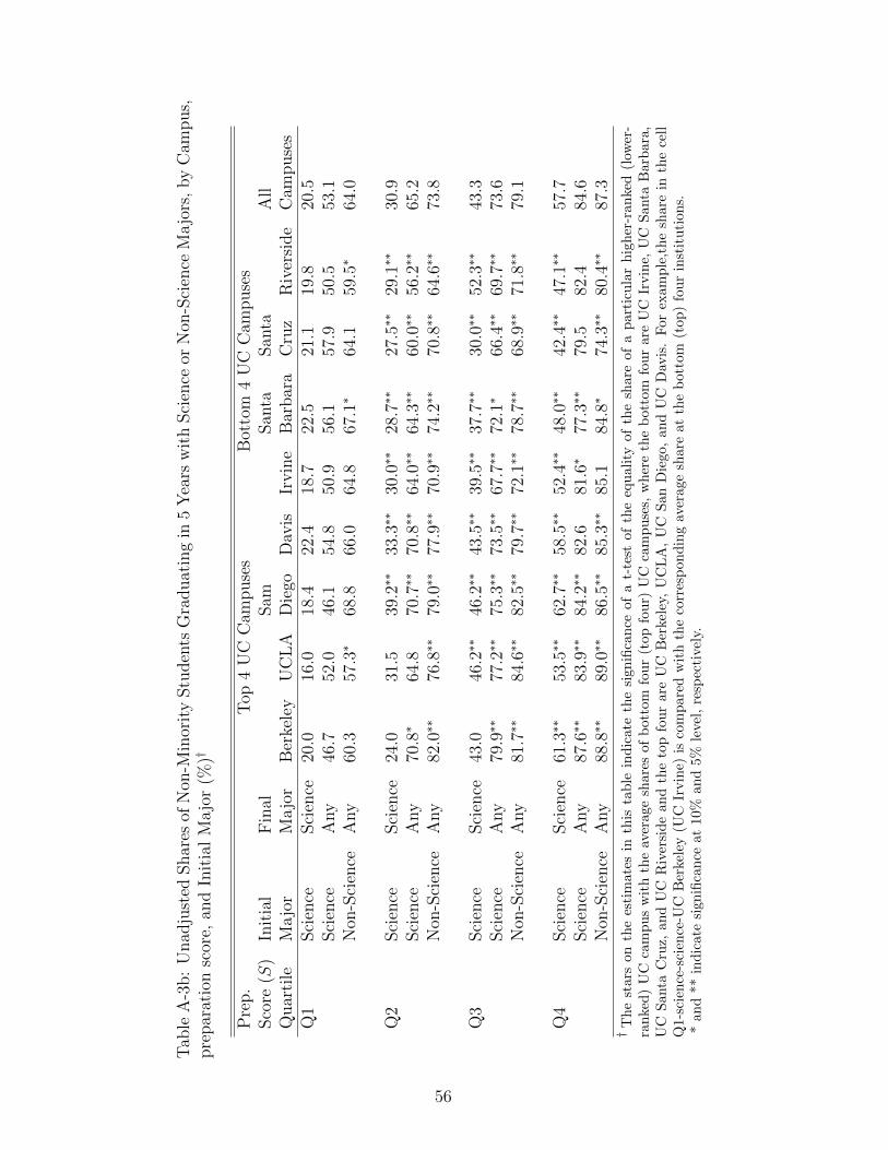
Tab

leA

-3b:

Unad

just

edShar

esof

Non

-Min

orit

yStu

den

tsG

raduat

ing

in5

Yea

rsw

ith

Sci

ence

orN

on-S

cien

ceM

ajo

rs,

by

Cam

pus,

pre

par

atio

nsc

ore,

and

Init

ial

Majo

r(%

)†

Pre

p.

Top

4U

CC

ampuse

sB

otto

m4

UC

Cam

puse

sSco

re(S

)In

itia

lF

inal

Sam

San

taSan

taA

llQ

uar

tile

Majo

rM

ajo

rB

erke

ley

UC

LA

Die

goD

avis

Irvin

eB

arbar

aC

ruz

Riv

ersi

de

Cam

puse

sQ

1Sci

ence

Sci

ence

20.0

16.0

18.4

22.4

18.7

22.5

21.1

19.8

20.5

Sci

ence

Any

46.7

52.0

46.1

54.8

50.9

56.1

57.9

50.5

53.1

Non

-Sci

ence

Any

60.3

57.3∗

68.8

66.0

64.8

67.1∗

64.1

59.5∗

64.0

Q2

Sci

ence

Sci

ence

24.0

31.5

39.2∗∗

33.3∗∗

30.0∗∗

28.7∗∗

27.5∗∗

29.1∗∗

30.9

Sci

ence

Any

70.8∗

64.8

70.7∗∗

70.8∗∗

64.0∗∗

64.3∗∗

60.0∗∗

56.2∗∗

65.2

Non

-Sci

ence

Any

82.0∗∗

76.8∗∗

79.0∗∗

77.9∗∗

70.9∗∗

74.2∗∗

70.8∗∗

64.6∗∗

73.8

Q3

Sci

ence

Sci

ence

43.0

46.2∗∗

46.2∗∗

43.5∗∗

39.5∗∗

37.7∗∗

30.0∗∗

52.3∗∗

43.3

Sci

ence

Any

79.9∗∗

77.2∗∗

75.3∗∗

73.5∗∗

67.7∗∗

72.1∗

66.4∗∗

69.7∗∗

73.6

Non

-Sci

ence

Any

81.7∗∗

84.6∗∗

82.5∗∗

79.7∗∗

72.1∗∗

78.7∗∗

68.9∗∗

71.8∗∗

79.1

Q4

Sci

ence

Sci

ence

61.3∗∗

53.5∗∗

62.7∗∗

58.5∗∗

52.4∗∗

48.0∗∗

42.4∗∗

47.1∗∗

57.7

Sci

ence

Any

87.6∗∗

83.9∗∗

84.2∗∗

82.6

81.6∗

77.3∗∗

79.5

82.4

84.6

Non

-Sci

ence

Any

88.8∗∗

89.0∗∗

86.5∗∗

85.3∗∗

85.1

84.8∗

74.3∗∗

80.4∗∗

87.3

†T

he

star

son

the

esti

mat

esin

this

tab

lein

dic

ate

the

sign

ifica

nce

of

at-

test

of

the

equ

ali

tyof

the

share

of

ap

art

icu

lar

hig

her

-ran

ked

(low

er-

ran

ked

)U

Cca

mp

us

wit

hth

eav

erag

esh

ares

ofb

ott

om

fou

r(t

op

fou

r)U

Cca

mp

use

s,w

her

eth

eb

ott

om

four

are

UC

Irvin

e,U

CS

anta

Barb

ara

,U

CS

anta

Cru

z,an

dU

CR

iver

sid

ean

dth

eto

pfo

ur

are

UC

Ber

kele

y,U

CL

A,

UC

San

Die

go,

an

dU

CD

avis

.F

or

exam

ple

,th

esh

are

inth

ece

llQ

1-sc

ien

ce-s

cien

ce-U

CB

erke

ley

(UC

Irvin

e)is

com

pare

dw

ith

the

corr

esp

on

din

gav

erage

share

at

the

bott

om

(top

)fo

ur

inst

itu

tion

s.*

and

**in

dic

ate

sign

ifica

nce

at10

%an

d5%

leve

l,re

spec

tivel

y.

56

Tab

leA

-4:

Log

itC

oeffi

cien

tsfo

rA

dm

issi

ons

by

UC

cam

pus†

San

taSan

taB

erke

ley

UC

LA

San

Die

goD

avis

Irvin

eB

arbar

aC

ruz

Riv

ersi

de

Min

orit

y3.

482∗∗

3.07

3∗∗

2.27

8∗∗

3.31

8∗∗

1.13

4∗∗

1.72

3∗∗

1.15

3∗∗

0.69

6∗∗

(0.0

39)

(0.0

35)

(0.0

42)

(0.0

56)

(0.0

39)

(0.0

43)

(0.0

52)

(0.0

49)

Min

orit

yX

Sci

ence

-1.3

84∗∗

-0.1

87∗∗

-0.2

64∗

0.01

7-0

.172

0.01

2-0

.132

-0.4

02∗∗

(0.0

59)

(0.0

73)

(0.1

06)

(0.1

36)

(0.1

18)

(0.1

62)

(0.1

77)

(0.1

76)

Pre

par

atio

nSco

re2.

343∗∗

3.02

5∗∗

3.66

6∗∗

3.23

5∗∗

2.57

8∗∗

3.46

9∗∗

2.27

4∗∗

2.18

8∗∗

(0.0

19)

(0.0

21)

(0.0

29)

(0.0

30)

(0.0

25)

(0.0

32)

(0.0

31)

(0.0

32)

Min

orit

yN

on-s

cien

ceA

dva

nta

gein

Pre

pSco

reU

nit

s1.

486

1.01

60.

622

1.02

60.

440

0.49

70.

507

0.31

8M

inor

ity

Sci

ence

Adva

nta

gein

Pre

pSco

reU

nit

s0.

895

0.95

40.

549

1.03

10.

373

0.50

00.

449

0.13

4†

Sep

arat

elo

gits

wer

ees

tim

ated

for

each

cam

pu

sw

her

eth

eou

tcom

ew

as

wh

eth

eror

not

the

stu

den

tw

as

ad

mit

ted

an

dth

esa

mp

lew

as

the

set

ofst

ud

ents

wh

oap

pli

edto

that

par

ticu

lar

cam

pus.

Ad

dit

ion

al

contr

ols

incl

uded

wer

e(i

)in

itia

lsc

ien

cem

ajo

r,(i

i)d

um

my

vari

ab

les

for

each

par

enta

lin

com

eca

tego

ry,

and

(iii

)d

um

my

vari

ab

les

for

each

pare

nta

led

uca

tion

cate

gory

.P

rep

ara

tion

score

isin

stan

dard

dev

iati

on

un

its.

Min

orit

yn

on-s

cien

cead

vanta

geis

calc

ula

ted

by

div

idin

gth

eco

effici

ent

on

min

ori

tyby

the

coeffi

cien

ton

the

pre

para

tion

score

.M

inori

tysc

ien

cead

vanta

geis

calc

ula

ted

by

sum

min

gth

eco

effici

ent

on

min

ori

tyan

dm

inori

tyti

mes

init

ial

scie

nce

ma

jor

an

dd

ivid

ing

by

the

coeffi

cien

ton

pre

par

atio

nsc

ore.

Sta

nd

ard

erro

rsin

par

enth

eses

.*

an

d**

ind

icate

sign

ifica

nce

at

10%

an

d5%

level

,re

spec

tive

ly.

57

Table A-5: Attendance decisions of minority students admitted to different pairs of UC campusesfor pre-Prop 209 period†

San Santa SantaBerkeley UCLA Diego Davis Irvine Barbara Cruz Riverside

Non-Minority (%):Berkeley - 53% 77% 82% 82% 86% 88% 83%UCLA 1739 - 76% 80% 81% 88% 90% 83%San Diego 821 1170 - 53% 65% 63% 71% 67%Davis 941 706 459 - 54% 55% 65% 63%Irvine 412 1151 426 355 - 50% 58% 64%Santa Barbara 723 1051 618 644 563 - 65% 62%Santa Cruz 587 384 285 466 210 747 - 45%Riverside 231 578 234 235 543 471 247 -Minority (%):Berkeley - 72% 84% 88% 89% 89% 90% 84%UCLA 6118 - 78% 81% 88% 89% 90% 83%San Diego 4335 5886 - 65% 75% 75% 78% 80%Davis 3551 2843 4303 - 66% 64% 73% 79%Irvine 1770 3896 3945 2619 - 62% 72% 81%Santa Barbara 1483 2380 3489 4103 3698 - 62% 69%Santa Cruz 1128 727 1472 2614 1083 3740 - 50%Riverside 639 1364 1627 1123 3502 1571 727 -† For Row A, Column B, value of cell is: Above diagonal: If admitted to Campus A and B, probabilityof attending campus A conditional on attending campus A or B. Below diagonal: Number in race-periodgroup admitted to Campus A and B and attended Campus A or B. (A student admitted to more than twocampuses will appear in this count multiple times)

58

Table A-6a: Nested Logit Coefficients: Dale-Krueger Controls 5-Year Graduation Criteria

Std. Coef. Std.Coef. Err. × URM Err.

Science IndexAdmitted × Berkeley 0.649∗∗ 0.175 0.011 0.247Admitted × UCLA 0.703∗∗ 0.165 -0.147 0.240Admitted × San Diego 0.563∗∗ 0.152 0.049 0.285Admitted × Davis 0.350 0.228 0.566 0.810Admitted × Irvine 0.471∗∗ 0.231 1.706∗∗ 0.711Admitted × Santa Barbara 0.089 0.265 1.429∗ 0.800Admitted × Santa Cruz 0.891 0.854 2.822 2.140Admitted × Riverside 1.471∗ 0.870 0.866 2.011Applied × Berkeley 0.052 0.083 -0.171 0.213Applied × UCLA -0.111 0.090 -0.130 0.220Applied × San Diego 0.198∗ 0.111 -0.252 0.265Applied × Davis 0.374∗ 0.208 -1.232 0.805Applied × Irvine -0.498∗∗ 0.232 -1.095 0.691Applied × Santa Barbara 0.102 0.275 -1.440∗ 0.799Applied × Santa Cruz -1.026 0.854 -2.308 2.128Applied × Riverside -1.416 0.869 -0.402 2.001Admitted Top × Rej. Mid. -0.464∗ 0.277 0.458 0.732Admitted Top × Rej. Low -0.124 0.133 -0.592∗∗ 0.285Applied Top × Rej. Mid. -0.293 0.239 1.251 0.781Applied Top × Rej. Low 0.582 0.607 1.571 1.578Applied Mid × Rej. Mid 0.294 0.937 0.057 1.736Non-Science IndexAdmitted × Berkeley 0.480∗∗ 0.164 0.052 0.212Admitted × UCLA 0.549∗∗ 0.161 -0.129 0.202Admitted × San Diego 0.493∗∗ 0.144 0.241 0.235Admitted × Davis 0.383∗ 0.201 -0.426 0.547Admitted × Irvine 0.303 0.207 0.832∗ 0.488Admitted × Santa Barbara -0.200 0.220 0.769 0.523Admitted × Santa Cruz 0.878 0.741 1.843 1.415Admitted × Riverside 1.138 0.762 1.446 1.358Applied × Berkeley -0.060 0.077 -0.155 0.181Applied × UCLA 0.089 0.085 -0.213 0.185Applied × San Diego 0.271∗∗ 0.101 -0.447∗∗ 0.214Applied × Davis 0.185 0.180 -0.282 0.538Applied × Irvine -0.433∗∗ 0.208 -0.219 0.462Applied × Santa Barbara 0.630∗∗ 0.233 -0.878∗ 0.523Applied × Santa Cruz -0.926 0.742 -1.231 1.394Applied × Riverside -1.169 0.762 -0.816 1.343Admitted Top × Rej. Mid. -0.198 0.250 0.292 0.538Admitted Top × Rej. Low -0.139 0.125 -0.501∗∗ 0.245Applied Top × Rej. Mid. -0.439∗∗ 0.210 0.634 0.538Applied Top × Rej. Low 0.565 0.525 1.255 1.072Applied Mid × Rej. Mid -0.101 0.813 0.068 1.284

* and ** indicate significance at 10% and 5% level, respectively.

59

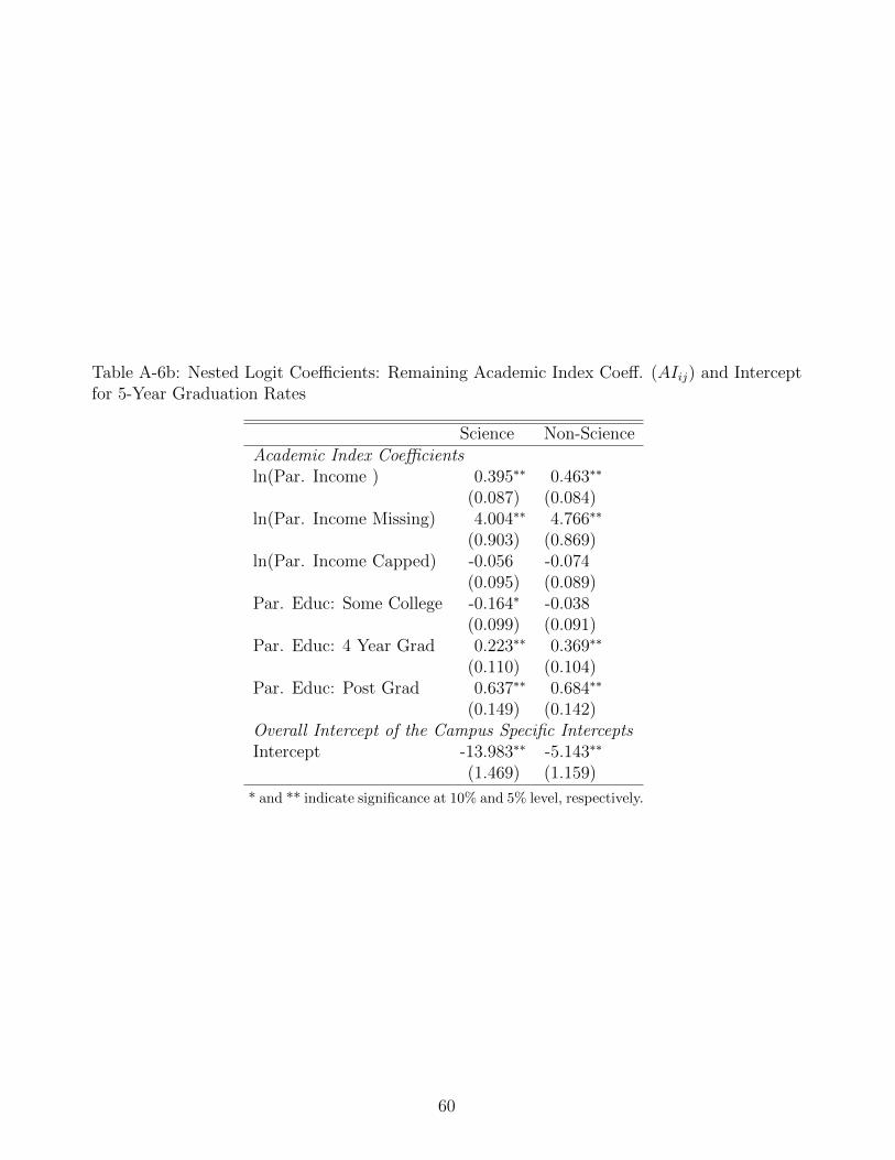
Table A-6b: Nested Logit Coefficients: Remaining Academic Index Coeff. (AIij) and Interceptfor 5-Year Graduation Rates

Science Non-ScienceAcademic Index Coefficientsln(Par. Income ) 0.395∗∗ 0.463∗∗

(0.087) (0.084)ln(Par. Income Missing) 4.004∗∗ 4.766∗∗

(0.903) (0.869)ln(Par. Income Capped) -0.056 -0.074

(0.095) (0.089)Par. Educ: Some College -0.164∗ -0.038

(0.099) (0.091)Par. Educ: 4 Year Grad 0.223∗∗ 0.369∗∗

(0.110) (0.104)Par. Educ: Post Grad 0.637∗∗ 0.684∗∗

(0.149) (0.142)Overall Intercept of the Campus Specific InterceptsIntercept -13.983∗∗ -5.143∗∗

(1.469) (1.159)

* and ** indicate significance at 10% and 5% level, respectively.

60

Table A-6c: Nested Logit: Switching Cost Coefficients 5-year Graduation Criteria

Coefficients Switching Cost:STEM Intercept 1.567∗∗

(0.431)Non STEM Intercept 1.740∗∗

(0.338)STEM × AIim -0.061∗∗

(0.026)Non STEM × AIih 0.001

(0.030)ln(Par. Income) 0.067∗∗

(0.022)ln(Par. Income Missing) 0.766∗∗

(0.231)ln(Par. Income Capped) 0.042

(0.036)Par. Educ: Some College 0.055

(0.043)Par. Educ: 4 Year Grad 0.072∗

(0.040)Par. Educ: Post Grad 0.024

(0.040)URM -0.055

(0.046)Asian -0.138∗∗

(0.029)UCLA -0.385∗∗

(0.062)San Diego 0.014

(0.041)Davis -0.183∗∗

(0.042)Irvine -0.313∗∗

(0.044)Santa Barbara -0.210∗∗

(0.051)Santa Cruz 0.060

(0.055)Riverside -0.294∗∗

(0.065)

* and ** indicate significance at 10% and 5%level, respectively.

61

Table A-7: Nested Logit Coefficients for Choice of Final Major based on 4-year GraduationCriteria

Non- Non-Science Science Science Science

Panel A: Net Returns Function:Campus-Specific Intercept Coefficients (φ1jk): Campus-Specific Slope Coefficients (φ2jk):UCLA -0.362 -1.972∗∗ UCLA × AIij 0.005 0.334∗∗

(0.935) (0.381) (0.059) (0.081)San Diego 3.69∗∗ -0.214 San Diego × AIij -0.203∗∗ 0.011

(0.821) (0.356) (0.048) (0.071)Davis 2.991∗∗ -0.361 Davis × AIij -0.203∗∗ -0.050

(0.816) (0.323) (0.048) (0.065)Irvine 3.064∗∗ 0.089 Irvine × AIij -0.192∗∗ -0.078

(0.856) (0.339) (0.051) (0.072)Santa Barbara 5.366∗∗ 0.458 Santa Barbara × AIij -0.326∗∗ -0.069

(0.832) (0.327) (0.047) (0.064)Santa Cruz 8.406∗∗ 2.109∗∗ Santa Cruz × AIij -0.537∗∗ -0.409∗∗

(0.923) (0.432) (0.048) (0.066)Riverside 5.727∗∗ 0.904∗∗ Riverside × AIij -0.325∗∗ -0.158∗∗

(0.866) (0.367) (0.048) (0.077)

Panel B: Academic Preparation Function (AIij):HS GPA 2.114∗∗ 1.020∗∗

(0.154) (0.111)SAT Math 9.469∗∗ -1.01∗∗

(0.559) (0.231)SAT Verbal 0.009∗∗ 2.417∗∗

(0.340) (0.271)URM -1.136∗∗ -0.851∗∗

(0.218) (0.128)Asian 0.048 -0.275∗∗

(0.053) (0.041)

Nesting parameterρ 0.407∗∗

(0.083)Log-Likelihood -54,670

All campus dummies are measured relative to UC Berkeley (the omitted category). The coefficients on φ1jk andφ2jk for UC Berkeley are normalized to zero and one, respectively.* and ** indicate significance at 10% and 5% level, respectively.

62

Table A-8a: Nested Logit Coefficients: Dale-Krueger Controls 4-year Graduation Criteria

Std. Coef. Std.Coef. Err. × URM Err.

Science IndexAdmitted × Berkeley 0.440∗∗ 0.088 0.305 0.258Admitted × UCLA 0.357∗∗ 0.082 0.438 0.276Admitted × San Diego 0.187∗ 0.095 -0.101 0.329Admitted × Davis 0.139 0.204 -0.419 0.923Admitted × Irvine 0.651∗∗ 0.221 1.126 0.849Admitted × Santa Barbara 0.144 0.278 0.909 1.031Admitted × Santa Cruz 0.431 0.887 19.267 53.033Admitted × Riverside 0.382 0.878 7.633 35.189Applied × Berkeley -0.096 0.059 -0.317 0.242Applied × UCLA -0.205∗∗ 0.067 -0.543∗∗ 0.266Applied × San Diego -0.159∗ 0.087 0.264 0.315Applied × Davis 0.059 0.200 0.386 0.919Applied × Irvine -0.724∗∗ 0.221 -0.699 0.844Applied × Santa Barbara -0.267 0.277 -0.746 1.027Applied × Santa Cruz -0.729 0.888 -19.059 53.033Applied × Riverside -0.443 0.878 -7.267 35.188Admitted Top × Rej. Mid. -0.503∗∗ 0.236 1.305 0.967Admitted Top × Rej. Low 0.076 0.094 -0.364 0.276Applied Top × Rej. Mid. 0.155 0.225 -0.025 0.988Applied Top × Rej. Low 0.249 0.655 -1.025 1.788Applied Mid × Rej. Mid -0.222 0.936 9.900 35.182Non Science IndexAdmitted × Berkeley 0.093 0.061 0.117 0.121Admitted × UCLA 0.181∗∗ 0.063 0.160 0.117Admitted × San Diego 0.100∗ 0.057 0.076 0.138Admitted × Davis 0.039 0.103 0.327 0.373Admitted × Irvine 0.091 0.112 1.002∗∗ 0.336Admitted × Santa Barbara -0.124 0.124 1.022∗∗ 0.375Admitted × Santa Cruz 0.882∗ 0.470 -0.095 0.930Admitted × Riverside 0.365 0.467 -0.375 0.912Applied × Berkeley -0.095∗∗ 0.038 -0.064 0.106Applied × UCLA 0.051 0.043 -0.240∗∗ 0.112Applied × San Diego -0.014 0.048 0.011 0.126Applied × Davis 0.009 0.098 -0.351 0.369Applied × Irvine -0.262∗∗ 0.113 -0.738∗∗ 0.327Applied × Santa Barbara 0.321∗∗ 0.125 -0.998∗∗ 0.372Applied × Santa Cruz -1.033∗∗ 0.473 0.436 0.927Applied × Riverside -0.515 0.467 0.699 0.911Admitted Top × Rej. Mid. -0.075 0.140 0.642∗ 0.376Admitted Top × Rej. Low 0.005 0.060 -0.242∗ 0.132Applied Top × Rej. Mid. -0.208∗ 0.114 0.303 0.368Applied Top × Rej. Low 0.350 0.324 0.166 0.736Applied Mid × Rej. Mid -0.175 0.504 -0.680 0.836

* and ** indicate significance at 10% and 5% level, respectively.

63

Table A-8b: Nested Logit Coefficients: Remaining Academic Index Coeff. (AIij) and Interceptfor 4-Year Graduation Rates

Science Non-ScienceAcademic Index Coefficientsln(Par. Income ) 0.202∗∗ 0.296∗∗

(0.044) (0.035)ln(Par. Income Missing) 2.314∗∗ 3.287∗∗

(0.474) (0.384)ln(Par. Income Capped) 0.028 -0.006

(0.061) (0.042)Par. Educ: Some College -0.111 0.035

(0.077) (0.051)Par. Educ: 4 Year Grad 0.026 0.132∗∗

(0.072) (0.049)Par. Educ: Post Grad 0.225∗∗ 0.239∗∗

(0.074) (0.053)Overall Intercept of the Campus Specific InterceptsIntercept -16.005∗∗ -4.743∗∗

(0.998) (0.570)

* and ** indicate significance at 10% and 5% level, respectively.

64

Table A-8c: Nested Logit: Switching Cost Coefficients 4-year Graduation Criteria

Coefficients Switching Cost:STEM Intercept 1.910∗∗

(0.422)Non STEM Intercept 1.912∗∗

(0.258)STEM × AIij -0.056∗∗

(0.028)Non STEM × AIij -0.050

(0.045)ln(Par. Income) 0.090∗∗

(0.032)ln(Par. Income Missing) 0.993∗∗

(0.339)ln(Par. Income Capped) 0.036

(0.049)Par. Educ: Some College -0.040

(0.063)Par. Educ: 4 Year Grad -0.039

(0.058)Par. Educ: Post Grad -0.070

(0.057)URM 0.022

(0.069)Asian -0.090∗∗

(0.040)UCLA -0.636∗∗

(0.050)San Diego 0.034

(0.057)Davis -0.211∗∗

(0.056)Irvine -0.295∗∗

(0.061)Santa Barbara -0.110

(0.071)Santa Cruz 0.095

(0.074)Riverside -0.315∗∗

(0.084)

* and ** indicate significance at 10% and 5%level, respectively.

65

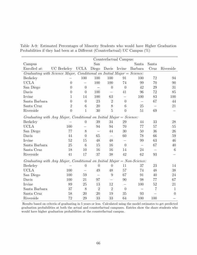
Table A-9: Estimated Percentages of Minority Students who would have Higher GraduationProbabilities if they had been at a Different (Counterfactual) UC Campus (%)

Counterfactual Campus:Campus San Santa SantaEnrolled at: UC Berkeley UCLA Diego Davis Irvine Barbara Cruz RiversideGraduating with Science Major, Conditional on Initial Major = Science:Berkeley − 100 100 100 91 100 72 94UCLA 0 − 100 100 74 99 70 90San Diego 0 0 − 0 0 42 29 31Davis 0 0 100 − 41 96 72 85Irvine 1 14 100 63 − 100 83 100Santa Barbara 0 0 23 2 0 − 67 44Santa Cruz 2 6 20 8 6 25 − 21Riverside 0 1 30 5 0 51 69 −

Graduating with Any Major, Conditional on Initial Major = Science:Berkeley − 0 39 34 29 44 33 28UCLA 100 − 94 94 70 77 57 55San Diego 77 8 − 44 30 50 36 26Davis 44 0 65 − 60 78 66 59Irvine 52 15 48 48 − 99 63 46Santa Barbara 25 6 15 16 0 − 67 40Santa Cruz 18 10 16 16 14 24 − 6Riverside 41 17 37 38 42 62 93 −

Graduating with Any Major, Conditional on Initial Major = Non-Science:Berkeley − 0 0 0 11 37 23 14UCLA 100 − 49 48 57 74 48 38San Diego 100 59 − 9 67 91 40 24Davis 100 21 97 − 90 98 77 67Irvine 89 25 13 12 − 100 52 21Santa Barbara 37 8 2 2 0 − 7 1Santa Cruz 58 20 20 19 35 93 − 0Riverside 72 29 33 33 64 100 100 −

Results based on criteria of graduating in 5 years or less. Calculated using the model estimates to get predictedgraduation probabilities at both the actual and counterfactual campuses. Entries show the share students whowould have higher graduation probabilities at the counterfactual campus.

66

Table A-10: Estimated Proportions of Non-Minority Students who would have Higher Gradua-tion Probabilities if they had been at a Different (Counterfactual) UC Campus (%)

Counterfactual Campus:Campus San Santa SantaEnrolled at: UC Berkeley UCLA Diego Davis Irvine Barbara Cruz RiversideGraduating with Science Major, Conditional on Initial Major = Science:Berkeley − 58 100 100 28 67 7 35UCLA 28 − 100 100 37 81 10 51San Diego 0 0 − 0 0 5 2 4Davis 0 0 100 − 3 66 18 43Irvine 12 43 100 92 − 100 49 91Santa Barbara 0 1 58 9 0 − 22 20Santa Cruz 11 21 58 34 25 64 − 57Riverside 12 21 72 35 9 89 39 −

Graduating with Any Major, Conditional on Initial Major = Science:Berkeley − 0 4 2 1 2 1 1UCLA 100 − 36 33 7 10 4 4San Diego 93 54 − 45 2 6 3 2Davis 89 36 66 − 8 20 10 7Irvine 75 40 82 78 − 95 31 22Santa Barbara 64 41 55 56 14 − 23 4Santa Cruz 54 37 50 50 47 62 − 26Riverside 59 43 60 58 60 83 61 −

Graduating with Any Major, Conditional on Initial Major = Non-Science:Berkeley − 0 0 0 0 2 1 0UCLA 100 − 7 7 8 13 5 3San Diego 100 92 − 61 10 37 4 2Davis 100 82 65 − 33 65 13 7Irvine 97 46 40 38 − 100 26 6Santa Barbara 85 44 17 17 0 − 1 0Santa Cruz 94 60 59 59 80 100 − 2Riverside 84 43 50 49 78 100 97 −

Results based on criteria of graduating in 5 years or less. Calculated using the model estimates to get predictedgraduation probabilities at both the actual and counterfactual campuses. Entries show the share students whowould have higher graduation probabilities at the counterfactual campus.

67

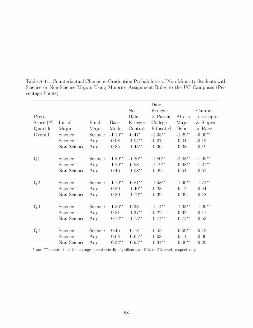
Table A-11: Counterfactual Change in Graduation Probabilities of Non-Minority Students withScience or Non-Science Majors Using Minority Assignment Rules to the UC Campuses (Per-centage Points)

Dale-No Krueger Campus

Prep. Dale- × Parent Altern. InterceptsScore (S) Initial Final Base Krueger College Major & SlopesQuartile Major Major Model Controls Educated Defn. × RaceOverall Science Science -1.10∗∗ -0.47∗ -1.03∗∗ -1.29∗∗ -0.95∗∗

Science Any -0.08 1.04∗∗ -0.07 0.04 -0.15Non-Science Any 0.35 1.45∗∗ 0.36 0.38 0.19

Q1 Science Science -1.89∗∗ -1.20∗∗ -1.80∗∗ -2.08∗∗ -1.95∗∗

Science Any -1.20∗∗ 0.58 -1.19∗∗ -0.98∗∗ -1.21∗∗

Non-Science Any -0.46 1.08∗∗ -0.49 -0.54 -0.57

Q2 Science Science -1.70∗∗ -0.81∗∗ -1.58∗∗ -1.90∗∗ -1.72∗∗

Science Any -0.30 1.40∗∗ -0.28 -0.12 -0.44Non-Science Any 0.39 1.79∗∗ 0.39 0.39 0.18

Q3 Science Science -1.23∗∗ -0.38 -1.14∗∗ -1.38∗∗ -1.09∗∗

Science Any 0.21 1.37∗∗ 0.22 0.32 0.11Non-Science Any 0.72∗∗ 1.73∗∗ 0.74∗∗ 0.77∗∗ 0.53

Q4 Science Science -0.46 -0.18 -0.43 -0.69∗∗ -0.13Science Any 0.08 0.65∗∗ 0.08 0.11 0.06Non-Science Any 0.32∗∗ 0.93∗∗ 0.34∗∗ 0.40∗∗ 0.20

* and ** denote that the change is statistically significant at 10% or 5% level, respectively.

68