university of alberta search for microscopic black … · in this multijet analysis, quantum...
TRANSCRIPT

CER
N-T
HES
IS-2
014-
114
05/0
9/20
14
University of Alberta
Search for Microscopic Black Holes in Multijet Final States with theATLAS Detector using 8 TeV Proton-Proton Collisions
at the Large Hadron Collider
by
Asif Saddique
A thesis submitted to the Faculty of Graduate Studies and Research inpartial fulfillment of the requirements for the degree of
Doctor of Philosophy
in
Experimental High Energy Physics
Department of Physics
c©Asif SaddiqueFall 2014
Edmonton, Alberta
Permission is hereby granted to the University of Alberta Libraries to reproduce single copies of thisthesis and to lend or sell such copies for private, scholarly or scientific research purposes only. Wherethe thesis is converted to, or otherwise made available in digital form, the University of Alberta will
advise potential users of the thesis of these terms.
The author reserves all other publication and other rights in association with the copyright in thethesis and, except as herein before provided, neither the thesis nor any substantial portion thereof
may be printed or otherwise reproduced in any material form whatsoever without the author’s priorwritten permission.

Dedicated
ToProfessor Riazuddin (RIP),
the father of physics in Pakistan,a great physicist and human being.

Abstract
Microscopic black holes are expected to produce a high multiplicity of Stan-
dard Model (SM) particles having large transverse momenta in the final
state. In this thesis, a search for microscopic black holes in multijet final
states with the ATLAS 2012 data using 8 TeV centre of mass energy of
proton-proton collisions at the Large Hadron Collider is performed in a
data sample corresponding to an integrated luminosity of 20.3 fb−1. The
search is simplified to multijet final states because most of the expected SM
particles produced from black hole decay would lead to hadronic jets. The
data events with high-transverse momenta have been analysed for different
exclusive jet multiplicities, i.e. 2, 3, ..., 7, and inclusive jet multiplicities, i.e.
≥ 3, 4, ..., 7. In this multijet analysis, Quantum Chromodynamics (QCD)
multijet production is the main background. For all the multijet final states,
the data distributions for the sum of jet transverse momenta (HT =∑pT )
in an event have been observed to be consistent with QCD expectations.
For inclusive multijet final states, model-independent and model-dependent
exclusion limits at a 95% confidence level are set on the production of new
physics and non-rotating black holes, respectively. The model-independent
upper limit on cross section times acceptance times efficiency is 0.29 fb to
0.14 fb for jet multiplicities ≥ 3 to ≥ 7 for HT > 4.0 TeV. The model-
dependent lower limits on minimum black hole mass are set for different
non-rotating black hole models.

Acknowledgements
In the name of Allah, the Most Gracious, the Ever Merciful. His kind
mercy made it possible to finish my thesis.
My deepest thanks and gratitude go to my supervisor Dr. Douglas
M. Gingrich for his support, patience, guidance and providing me an ex-
cellent research environment. His flexible attitude always provided a space
to work independently, and his professional skills allowed for timely guid-
ance for me. I would also like to thank all of the CPP faculty and staff
members for creating a comfortable working atmosphere. I also appreciate
all the facilities and the wonderful learning environment provided by the
Department of Physics at the University of Alberta.
Because of the help and great support of kind people around me,
the task of finishing my thesis became easier and achievable. I would espe-
cially thank my senior colleague and postdoctoral fellow Dr. Francesc Vives
Vaque, whose polite and encouraging attitude always helped me a lot to
boost this work. Besides work, my wife Fauzia Sadiq and I always enjoyed
family gatherings with his family.
I would like to acknowledge my current and ex-fellows in the ATLAS
Alberta group: Patrick, Andrew, Samina, Nooshin, Kingsley and especially
Aatif Imtiaz Butt and Dr. Halasya Siva Subramania for having useful dis-
cussions with me regarding this work.
I would like to thank my ex-supervisor Dr. James Pinfold for his
support and supervision in the initial phase of my PhD. I also thank my
ex-colleagues Long Zhang and Dr. Nitesh Soni for providing me help to
train myself in doing data analysis. I, and my wife also, have a lot of good
memories of spending time with Nitesh’s family.
How can I forget one of impressive personalities whom I met in
Canada, Logan Sibley. I learned one thing from him – how to sacrifice your
time to help people around you. I also thank him for spending his time for
doing a careful proof reading of this thesis.

I am thankful to all of my family friends, Atif, Asad, Omer, Zawar,
Jamil, Nadia, Amna andTayyaba, who made our stay enjoyable in Canada.
We have had several trips and gatherings during my studies in Canada.
Thanks for your wonderful company.
I would love to acknowledge my beloved wife for her caring attitude
and moral support in all aspects of my life. She is a wonderful life partner.
I would also deeply thank my mother, father (RIP), brothers and sisters
for praying and encouraging me to move forward in my life, especially my
mother, who always remained worried and loving for me.

Table of Contents
1 Introduction 1
2 Standard Model Physics and Beyond 5
2.1 Introduction . . . . . . . . . . . . . . . . . . . . . . . . . . . 5
2.2 The Standard Model of Particle Physics . . . . . . . . . . . 6
2.2.1 Electroweak Theory and Higgs Mechanism . . . . . . 8
2.2.2 Limitations of the Standard Model . . . . . . . . . . 11
2.3 Physics Beyond the Standard Model . . . . . . . . . . . . . 12
2.3.1 Theories of Extra Dimensions . . . . . . . . . . . . . 12
2.4 Microscopic Black Hole Physics . . . . . . . . . . . . . . . . 18
2.4.1 Production of Black Holes . . . . . . . . . . . . . . . 18
2.4.2 Production Cross Section of Black Holes . . . . . . . 21
2.4.3 The Nature of Black Holes . . . . . . . . . . . . . . . 23
2.4.4 Decay of Black Holes . . . . . . . . . . . . . . . . . . 26
2.5 Microscopic Black Holes at the LHC . . . . . . . . . . . . . 31
2.5.1 Cross Section and Extra Dimensions . . . . . . . . . 31
2.5.2 Hawking Temperature . . . . . . . . . . . . . . . . . 32
2.5.3 Measurement of Mass . . . . . . . . . . . . . . . . . . 32
2.5.4 Missing Energy in Black Hole Searches . . . . . . . . 33
2.5.5 Current Limits on MD . . . . . . . . . . . . . . . . . 34
2.5.6 Decay of Black Holes at the LHC . . . . . . . . . . . 35
3 The ATLAS Detector at the Large Hadron Collider 37
3.1 Introduction . . . . . . . . . . . . . . . . . . . . . . . . . . . 37
3.2 The Large Hadron Collider . . . . . . . . . . . . . . . . . . . 37
3.3 The ATLAS Detector . . . . . . . . . . . . . . . . . . . . . . 38
3.4 Inner Detector . . . . . . . . . . . . . . . . . . . . . . . . . . 40
3.5 Calorimeters . . . . . . . . . . . . . . . . . . . . . . . . . . . 41
3.5.1 Liquid Argon Calorimeter . . . . . . . . . . . . . . . 42
3.5.2 Hadronic Calorimeter . . . . . . . . . . . . . . . . . . 43

3.6 Muon Spectrometers . . . . . . . . . . . . . . . . . . . . . . 44
3.7 Forward Detectors . . . . . . . . . . . . . . . . . . . . . . . 45
3.8 Luminosity Measurement . . . . . . . . . . . . . . . . . . . . 46
3.9 Triggers and Data Acquisition . . . . . . . . . . . . . . . . . 48
4 Analysis 49
4.1 Introduction . . . . . . . . . . . . . . . . . . . . . . . . . . . 49
4.2 Monte Carlo Simulations . . . . . . . . . . . . . . . . . . . . 50
4.2.1 QCD Background Samples . . . . . . . . . . . . . . 51
4.3 Trigger . . . . . . . . . . . . . . . . . . . . . . . . . . . . . . 52
4.4 Data Selection . . . . . . . . . . . . . . . . . . . . . . . . . . 54
4.4.1 Event Selection . . . . . . . . . . . . . . . . . . . . . 57
4.4.2 Jet Selection . . . . . . . . . . . . . . . . . . . . . . . 57
4.5 Data Characteristics . . . . . . . . . . . . . . . . . . . . . . 58
4.5.1 The HT Distributions . . . . . . . . . . . . . . . . . . 61
4.5.2 Shape Invariance of Kinematic Distributions . . . . . 61
4.5.3 The Signal and the Control Regions . . . . . . . . . . 73
4.5.4 The Background Estimation . . . . . . . . . . . . . . 74
4.5.5 Correction to the Background Estimation . . . . . . . 76
4.6 Systematic Uncertainties . . . . . . . . . . . . . . . . . . . . 80
4.6.1 Corrections to Non-Invariance . . . . . . . . . . . . . 83
4.6.2 Choice of Normalisation Region . . . . . . . . . . . . 90
4.6.3 Jet Energy Uncertainties . . . . . . . . . . . . . . . . 91
4.6.4 Summary of Systematics . . . . . . . . . . . . . . . . 95
4.7 Exclusion Limits . . . . . . . . . . . . . . . . . . . . . . . . 96
4.7.1 Model-Independent Limits . . . . . . . . . . . . . . . 99
4.7.2 Model-Dependent Limits . . . . . . . . . . . . . . . . 100
5 Summary 110
Appendices 113
A Other Contribution to the ATLAS Experiment 114
B Trigger Study 116
C Event Selection 119
C.1 Event Cleaning . . . . . . . . . . . . . . . . . . . . . . . . . 119
C.1.1 Data Quality . . . . . . . . . . . . . . . . . . . . . . 119
C.1.2 Bad and Corrupt Events . . . . . . . . . . . . . . . . 120

C.1.3 Vertex Requirement . . . . . . . . . . . . . . . . . . . 120
C.1.4 Jet Quality . . . . . . . . . . . . . . . . . . . . . . . 120
C.1.5 Analysis Requirements . . . . . . . . . . . . . . . . . 121
C.2 CutFlow . . . . . . . . . . . . . . . . . . . . . . . . . . . . . 122
D Jet Kinematic Distributions 124
E Pileup Study 128
E.0.1 Number of Primary Vertices (NPV) . . . . . . . . . . 128
E.0.2 Average Interactions per Beam Crossing (µ) . . . . . 131
E.0.3 Choice of jet pT > 50 GeV . . . . . . . . . . . . . . . 131

List of Tables
2.1 xmin = E/MD as a function of n extra dimensions. . . . . . . 20
2.2 Number of degrees of freedom (dof) of the Standard Model
particles. . . . . . . . . . . . . . . . . . . . . . . . . . . . . . 28
2.3 Relative emissivities per degree of freedom for SM particles. 29
2.4 Probability of emission of SM particles. . . . . . . . . . . . . 30
2.5 Lower limits on MD at the 95 % confidence level. . . . . . . 35
3.1 Rapidities of the ATLAS forward detectors. . . . . . . . . . 46
4.1 Specifications of PYTHIA8 dijet MC weighted samples. . . . . 52
4.2 Specifications of HERWIG++ dijet MC weighted samples. . . 53
4.3 Comparison of PYTHIA8 and HERWIG++ QCD MCs. . . . . 53
4.4 The parameters extracted from the straight line fits to the
HT ratios, in the normalisation region, with respect to the
jet multiplicity N = 2, for the data and dijet MCs. . . . . . 72
4.5 The values of fit parameters (pi) along with errors (∆pi) for
the function f(x) = p0(1−x)p1
xp2+p3 ln x fitted to the dijet HT distribu-
tion for the ATLAS 2012 data. . . . . . . . . . . . . . . . . . 75
4.6 Number of the data and background entries, in the signal re-
gion, are shown as a function of HminT , for the jet multiplicity
N ≥ 3. The MC-based correction factors are also shown with
their corresponding uncertainties. . . . . . . . . . . . . . . 85
4.7 Number of the data and background entries, in the signal re-
gion, are shown as a function of HminT , for the jet multiplicity
N ≥ 4. The MC-based correction factors are also shown with
their corresponding uncertainties. . . . . . . . . . . . . . . 86
4.8 Number of the data and background entries, in the signal re-
gion, are shown as a function of HminT , for the jet multiplicity
N ≥ 5. The MC-based correction factors are also shown with
their corresponding uncertainties. . . . . . . . . . . . . . . . 87

4.9 Number of the data and background entries, in the signal re-
gion, are shown as a function of HminT , for the jet multiplicity
N ≥ 6. The MC-based correction factors are also shown with
their corresponding uncertainties. . . . . . . . . . . . . . . . 88
4.10 Number of the data and background entries, in the signal re-
gion, are shown as a function of HminT , for the jet multiplicity
N ≥ 7. The MC-based correction factors are also shown with
their corresponding uncertainties. . . . . . . . . . . . . . . . 89
4.11 The uncertainty due to the choice of the normalisation region. 92
4.12 Model-independent observed and expected upper limits on
cross section times acceptance times efficiency. . . . . . . . . 102
4.13 A comparison of model-independent upper limits at the 95%
confidence level on cross section times acceptance times effi-
ciency between the CMS and ATLAS results. . . . . . . . . 104
4.14 A comparison of model-dependent lower limits at the 95%
confidence level on minimum black hole mass between the
CMS and ATLAS results. . . . . . . . . . . . . . . . . . . . 109
C.1 Cut flow for the data and dijet MCs. . . . . . . . . . . . . . 122
C.2 Cut flow for the the data-periods. . . . . . . . . . . . . . . . 123
E.1 Average jet multiplicity, as a function of jet pT and NPV,
for the data. . . . . . . . . . . . . . . . . . . . . . . . . . . . 129
E.2 Average jet multiplicity, as a function of jet pT and µ, for
the data. . . . . . . . . . . . . . . . . . . . . . . . . . . . . . 132

List of Figures
2.1 Two (3+1)-spacetime branes embedded in a five dimensional
spacetime. . . . . . . . . . . . . . . . . . . . . . . . . . . . . 17
3.1 The maximum instantaneous luminosity and the cumula-
tive integrated luminosity delivered by the LHC per day and
recorded by ATLAS per day for pp collisions at 8 TeV centre
of mass energy. . . . . . . . . . . . . . . . . . . . . . . . . . 38
3.2 Schematic view of the ATLAS detector. . . . . . . . . . . . . 39
3.3 Cut-away view of ATLAS Inner Detector (ID). . . . . . . . . 41
3.4 The ATLAS calorimeters. . . . . . . . . . . . . . . . . . . . 42
3.5 Drawing of barrel module of the LAr calorimeter. . . . . . . 43
3.6 Layout of Muon Spectrometer. . . . . . . . . . . . . . . . . . 46
4.1 The EF j170 a4tchad ht700 trigger efficiency as a function
of pT and HT . . . . . . . . . . . . . . . . . . . . . . . . . . . 55
4.2 The EF j170 a4tchad ht700 trigger efficiency. . . . . . . . . . 56
4.3 The jet pT distributions for the exclusive jet multiplicities,
N = 2, 3, ..., 7, for the data and dijet MCs. . . . . . . . . . . 59
4.4 The jet η distributions of for the exclusive multiplicities, N =
2, 3, ..., 7, for the data and dijet MCs. . . . . . . . . . . . . . 60
4.5 The HT distributions for the exclusive jet multiplicity cases,
N = 2, 3, ..., 7, for the data and dijet MCs. . . . . . . . . . 62
4.6 The HT distributions for the inclusive jet multiplicity cases,
N ≥ 2, 3, ..., 7, for the data and dijet MCs. . . . . . . . . . 63
4.7 The HT ratios of the exclusive jet multiplicities N = 3, 4, .., 7
to the jet multiplicity N = 2, for the data and dijet MCs. . . 65
4.8 The HT ratios of the inclusive jet multiplicities N ≥ 3, 4, .., 7
to the jet multiplicity N = 2, for the data and dijet MCs. . . 66
4.9 The HT ratios of the exclusive jet multiplicities N = 3, 4, .., 7
to the jet multiplicity N = 2, in the normalisation region,
for the data and dijet MCs. . . . . . . . . . . . . . . . . . . 68
4.10 The HT ratios of the inclusive jet multiplicities N ≥ 3, 4, .., 7
to the jet multiplicity N = 2, in the normalisation region,
for the data and dijet MCs. . . . . . . . . . . . . . . . . . . 69
4.11 The slopes extracted from the HT ratios with respect to the
jet multiplicity N = 2, in the normalisation region, for the
data and dijet MCs. . . . . . . . . . . . . . . . . . . . . . . 70
4.12 The slopes extracted from the HT ratios with respect to the
jet multiplicity N = 3, in the normalisation region, for the
data and dijet MCs. . . . . . . . . . . . . . . . . . . . . . . 71
4.13 The background estimation for the HT distributions with 3σ
uncertainty, for the exclusive jet multiplicities N = 2, 3, ..., 7. 77
4.14 The background estimation for the HT distributions with 3σ
uncertainty, for the inclusive jet multiplicities N ≥ 2, 3, ..., 7. 78
4.15 The background estimations from the uncorrected and cor-
rected fits, in the signal region, for the exclusive jet multi-
plicities N = 3, 4, .., 7. . . . . . . . . . . . . . . . . . . . . . 81
4.16 The background estimations from the uncorrected and cor-
rected fits, in the signal region, for the inclusive jet multi-
plicities N ≥ 3, 4, .., 7. . . . . . . . . . . . . . . . . . . . . . 82
4.17 The gaussian distribution of ∆JERi corresponding to differ-
ent HminT , for the jet multiplicities N ≥ 3. . . . . . . . . . . . 94
4.18 The HminT distributions for the data, and the predicted back-
ground along with total uncertainty. . . . . . . . . . . . . . . 97
4.19 The HminT distributions for the data, and the predicted back-
ground along with total uncertainty. . . . . . . . . . . . . . . 98
4.20 Model-independent limits on upper cross section times ac-
ceptance times efficiency at the 95% confidence level, as a
function of HminT . . . . . . . . . . . . . . . . . . . . . . . . . 101
4.21 Model-independent limits on upper cross section times ac-
ceptance times efficiency at the 95% confidence level, as a
function of inclusive jet multiplicity. . . . . . . . . . . . . . . 103
4.22 CHARYBDIS2black hole samples for different numbers of ex-
tra dimensions n. . . . . . . . . . . . . . . . . . . . . . . . . 105
4.23 CHARYBDIS2black hole samples for different black hole mass
thresholds Mth. . . . . . . . . . . . . . . . . . . . . . . . . . 106
4.24 The upper limit on the cross section at the 95% confidence
level, as a function of MD. . . . . . . . . . . . . . . . . . . . 107

4.25 The upper limit on cross section at the 95% confidence level,
as a function of Mth. . . . . . . . . . . . . . . . . . . . . . . 108
B.1 The EF j170 a4tchad ht700 trigger efficiency as a function
of HT and jet multiplicity. . . . . . . . . . . . . . . . . . . . 117
B.2 The EF j170 a4tchad ht700 trigger efficiency as a function
of HT , µ and NPV. . . . . . . . . . . . . . . . . . . . . . . . 118
D.1 The jet φ distributions, for the exclusive jet multiplicities
N = 2, 3, ..., 7, for the data and dijet MCs. . . . . . . . . . 125
D.2 The first leading jet pT distributions, for the exclusive jet
multiplicities N = 2, 3, ..., 7, for the data and dijet MCs. . . 126
D.3 The second leading jet pT distributions, for the exclusive jet
multiplicities N = 2, 3, ..., 7, for the data and the dijet MCs. 127
E.1 Average jet multiplicity, as a function of NPV and jet pT ,
for the data. . . . . . . . . . . . . . . . . . . . . . . . . . . . 130
E.2 Average jet multiplicity, as a function of µ and jet pT , for
the data. . . . . . . . . . . . . . . . . . . . . . . . . . . . . . 132
E.3 The HT ratios, as a function of NPV, for the data. . . . . . 134
E.4 The HT ratios, as a function of µ, for the data. . . . . . . . 134

List of Abbreviations and Symbols
ALFA Absolute Luminosity For ATLAS
ALICE A Large Ion Collider Experiment
ATLAS A Toroidal LHC Apparatus
BCM Beam Condition Monitor
BX Bunch Crossing
CDF Collider Detector at Fermilab
CERN European Organization for Nuclear Research
CF Correction Factor
CL Confidence Level
CMS Compact Muon Solenoid
CR Control Region
CTEQ Coordinated Theoretical-Experimental project on QCD
D0 D-Zero Experiment at Fermilab
DSID Data Set IDentifier
EF Event Filter
EM ElectroMagnetic
FCAL Forward CALorimeter
GRL Good Run List
HEC Hadronic Endcap Calorimeter
ID Inner Detector
IP Interaction Point
JER Jet Energy Resolution
JES Jet Energy Scale
LAr Liquid Argon

LHC Large Hadron Collider
LO Leading Order
LUCID LUminosity measurement using Cerenkov Integrating Detector
MBTS Minimum Bias Trigger Scintillator
MC Monte Carlo
MDT Muon Drift Tube
MSSM Minimal Supersymmetric Standard Model
NLO Next to Leading Order
NMSSM Next to Minimal Supersymmetric Standard Model
NNLO Next to Next to Leading Order
NPV Number of Primary Vertices
NR Normalization Region
PDF Parton Distribution Function
QCD Quantum ChromoDynamics
QED Quantum ElectroDynamics
QFT Quantum Field Theory
RMS Root Mean Square
ROI Region Of Interest
RPC Resistive Plate Chamber
SCT Silicon Central Tracker
SM Standard Model
SR Signal Region
SUSY Supersymmetry
TGC Thin Gap Chamber
TRT Transition Radiation Tracker
ZDC Zero Degree Calorimeter

n Number of extra spatial dimensions
D Sum of four usual and number of extra dimensions, i.e. D = 4 + n
MEW Electroweak scale
MP Planck scale (in 4 D)
MD Multidimensional or true Planck scale
MBH Black hole mass
R Size of extra dimension
A (ω) Grey body factor of a black hole
lP Planck length corresponding to MP
lD Planck length corresponding to MD
rH Event horizon radius of a black hole
pT Transverse momentum of a jet
HT Sum of the jet transverse momenta
N Number of jets in the final state or jet multiplicity
η Pseudorapidity
φ Azimuthal angle around the beam axis
µ Number of interactions per bunch crossing
σ Total Cross section

Chapter 11
Introduction2
The large difference between the electroweak (MEW ∼ 0.1 TeV1) and the3
Planck scales (MP ∼ 1016 TeV) is known as the hierarchy problem. In other4
words, gravity appears to be very weak as compared to the SM forces. Tech-5
nically, the problem can also be expressed in terms of the large difference6
between the physical Higgs boson mass and the Planck mass. The physical7
Higgs boson mass lies near the electroweak scale, which is much smaller8
than the Planck mass. If the SM is valid up to the Planck scale then the9
bare mass of the Higgs boson has a natural value of order of the Planck10
scale. In this case, an incredible fine tuning (∼ 1017) of the cancellation11
of the radiative corrections and the bare Higgs boson mass is required to12
obtain a low value for the physical Higgs boson mass to the order of the13
electroweak scale. The hierarchy problem can also be solved if new gravi-14
tational physics exists near the electroweak scale. In this scenario, a new15
fundamental Planck scale of the order of the electroweak scale is defined.16
The contribution from the radiative corrections to the bare Higgs boson17
mass is much smaller than the previous case. Hence a large tuning of the18
corrections and the bare Higgs boson mass is not required to solve the19
hierarchy problem.20
1 It is assumed ~ = c = 1 throughout this thesis.
1

The production of microscopic black holes in the high energy proton-21
proton (pp) collisions at the LHC is one of the most exciting predictions of22
low-scale quantum gravity models [1–5]. These models are motivated by the23
hierarchy problem and explain the weakness of gravity as compared to the24
other SM forces. According to some of the low-scale gravity models [1–3],25
gravity is the only force that propagates in the extra dimensions (n) while26
the other forces are confined to the four observed dimensions. Therefore,27
the apparent gravity measured in the four dimensional physical world cor-28
responding to the large Planck scale MP is always much weaker than the29
actual gravity measured in D = 4+n dimensions corresponding to the true30
Planck scale (MD). The low-scale (∼ TeV) gravity would appear strong31
enough to be compared to the other SM forces and, as a consequence, the32
formation of the massive and extra-dimensional objects such as microscopic33
black holes may occur at the LHC.34
In this thesis, a microscopic black hole search based on the predic-35
tions of low-scale gravity models in high energy pp collisions with 8 TeV36
centre of mass energy (√s) at the LHC collected by the ATLAS detector37
in the year 2012 will be presented. The data correspond to a total inte-38
grated luminosity of 20.3 fb−1 with a luminosity uncertainty of 2.8%2. The39
low-scale gravity models predict that short-lived (∼ 10−27 sec) microscopic40
black holes would decay in the detectors and leave some distinguishable41
signature such as events with high multiplicities (number of particles in42
the final states) and high transverse momenta (pT ). The black hole decay43
produces particles primarily according to the SM degrees of freedom (num-44
ber of charge, spin, flavour and color states), which mainly leads to jets45
of hadrons in the final states. Therefore, our search for microscopic black46
holes is focussed on multijet final states. Observations of such multijet final47
2 The uncertainty in luminosity for the ATLAS 2012 data is derived by using the samemethod adopted for the 2011 ATLAS data, which is shown in Ref. [6].
2

states having high pT may provide valuable information about the nature of48
black holes, the dimensionality of space-time and the fundamental Planck49
scale.50
The main variable chosen for this study is HT , the scalar sum of51
pT of jets in an event. The HT distributions are expected to have the52
same shape for different jet multiplicities for the main QCD background53
in this study [7–10]. This shape invariance with multiplicity is the key54
assumption of this analysis used to estimate the QCD background for the55
expected microscopic black hole signals at the LHC.56
In chapter 2, SM physics and motivations for the physics beyond57
the SM are discussed. The theories with extra dimensions are important58
candidates for the potential extension of the SM, and predict the produc-59
tion of microscopic black holes at the LHC. Since a search for microscopic60
black holes at the LHC is the main scope of this thesis, microscopic black61
hole physics is briefly described along with some practical implications for62
observing them at the LHC.63
Chapter 3 is dedicated to the description of the LHC and the ATLAS64
detector at the CERN. Various sub-detectors of the ATLAS detector are65
discussed according to their functionality, importance and use in this study.66
The trigger and the data collection system of the ATLAS detector are also67
discussed at the end of chapter 3.68
Chapter 4 presents the main analysis, illustrating the necessary69
tools, assumptions, procedure and results of the study for the search of70
microscopic black holes in multijet final states of the ATLAS 2012 dataset.71
The data used in the analysis are studied for different jet multiplicities72
with the assumption of HT shape invariance with jet multiplicity for QCD73
events, which is directly determined from the data with corrections due to74
the effects of non-invariance derived from MC simulations. A summary of75
3

the study will be made by showing model-independent limits on the pro-76
duction of new physics and model-dependent limits on the production of77
microscopic black holes. The overall summary of the analysis is discussed78
in chapter 5. In addition to the primary analysis, my other contributions79
to the ATLAS experiment are described in appendix A.80
4

Chapter 281
Standard Model Physics and Beyond82
2.1 Introduction83
The SM is the most established theoretical framework of particle physics.84
Many modern particle detectors, for example ATLAS and CMS at the LHC85
have not found any evidence against the foundations of the SM. This theory86
has enjoyed many major experimental successes, like the discovery of W±87
and Z0 bosons, the top quark, and now the discovery of Higgs boson.88
The SM is not a “theory of everything” because it neither incorpo-89
rates gravity nor does it explain many open questions, for example, why the90
weak force is 1032 times stronger than the gravitational force, the matter-91
antimatter asymmetry, the nature of dark matter and dark energy, the92
strong CP problem and neutrino oscillations. These are the primary rea-93
sons to build theoretical models beyond the SM of particle physics.94
In this chapter, a brief introduction to the SM and its major limita-95
tions will be described along with some theories beyond the SM. There are96
many possible extensions of the SM and the theory of large extra dimen-97
sions is one of the important candidates. The production of microscopic98
black holes is an important consequence of the theory of large extra dimen-99
sions, which is the model used in this thesis. The physics of microscopic100
black holes will be discussed by describing their production, nature and de-101
cay. In the last section of this chapter, the observables that might show the102
5

possible signatures of microscopic black holes at the LHC will be described.103
2.2 The Standard Model of Particle Physics104
The SM of particle physics is the theory that describes the role of the fun-105
damental particles and interactions between them. All the known matter is106
composed of particles from the SM. There are two types of particles in the107
SM, the fundamental fermions (leptons, quarks and their antiparticles) and108
the fundamental bosons (gauge bosons and the Higgs boson). The fermions109
are half-integer spin particles, whereas bosons are integer spin particles.110
There are six leptons classified in three generations. The electron (e) and111
the electron neutrino (νe) are in the first generation, the muon (µ) and112
the muon neutrino (νµ) are in the second generation and the tau (τ) and113
the tau neutrino (ντ ) make the third generation. Similarly, there are six114
quarks in three generations, up (u) and down (d) in the first generation,115
strange (s) and charm (c) in the second generation and bottom (b) and116
top (t) in the third generation. Each quark can have three colours, red (r),117
green (g) and blue (b), but no free colour charge exists in nature at long118
distances. Except for the special case of the top quark1, quarks only appear119
in bound states called hadrons like the proton (uud) and pion (ud).120
There are four fundamental interactions in nature: the electromag-121
netic, the weak, the gravitational and the strong force. Every interaction122
has mediators: the photon for the electromagnetic force, two W ’s and a Z123
boson for the weak force, eight gluons for the strong force and maybe the124
graviton for gravity. The gluons themselves carry colour and anti-colour125
and therefore do not exist as isolated particles, but they can exist within126
hadrons or in colourless combinations (glueballs). Although the SM does127
not expain gravity, it has incorporated the other known forces into a sin-128
1 The mean lifetime of top quark is predicted to be 5× 10⁻²⁵ s [11], which is shorterthan the timescale for strong interactions, and therefore it does not form hadrons.
6

gle model. This model has achieved many experimental successes over the129
years and provided significant predictions, such as the existence of the top130
quark, and the masses of the weak force carriers.131
The SM forces are governed by three gauge theories, Quantum Elec-132
trodynamics (QED), Quantum Chromodynamics (QCD), and Electroweak133
interactions from the Glashow-Weinberg-Salam model. The Standard Model134
is a gauge theory based on the product group SUC(3)×SUL(2)×UY (1) as-135
sociated with the colour (C), weak and hypercharge (Y ) symmetries. The136
subscript L indicates that the charged weak interaction involves couplings137
only to the chiral left-handed component of the fermion. In the SM, all the138
gauge theories are required to be invariant under global and local gauge139
transformations.140
QED is an abelian and renormalisable gauge theory with symme-141
try group U(1). This theory describes the interactions between spin-1/2142
charged particles, the electromagnetic interactions. The theory provides143
a description of the interactions between two charged particles by the ex-144
change of a field quantum, the photon.145
QCD is a non-abelian and renormalisable gauge theory based on146
SU(3) group that describes the interaction of quarks via gluons. The non-147
abelian nature of the SU(3) group results in self interaction terms of gluons148
generating three and four-gluon vertices in the theory, which leads to a149
strong coupling, large at low energies and small at high energies. As a150
consequence QCD has two important features, confinement and asymptotic151
freedom. According to confinement, the quarks generally are confined in152
hadrons and an infinite amount of energy is required to separate a quark153
to infinity from its hadron. For example, if the quark and antiquark move154
far enough apart in a meson, then field energy increases to produce two155
new mesons instead of creating two free quarks. According to asymptotic156
7

freedom, the strength of strong coupling is small at very small distances157
such that quarks and gluons interact weakly and behave as free.158
Electroweak theory is a unified description of the electromagnetic159
and weak interactions. The massive gauge bosons are the mediators of the160
weak force. The fermions (leptons and quarks) and the gauge bosons are161
required to be massless in gauge theories. The massive leptons and quarks,162
and W± and Z gauge bosons, are accommodated in the gauge theories by163
the Higgs mechanism. Accordingly the local symmetry of the gauge group164
SUL(2)×UY (1) is spontaneously broken and a Higgs field is generated that165
interacts with other fields to produce not only the massive gauge bosons,166
but also the masses of leptons and quarks. The mechanism also postulates167
the existence of a massive scalar particle known as the Higgs boson.168
2.2.1 Electroweak Theory and Higgs Mechanism169
The electroweak gauge theory is the unified description of electromag-170
netic and weak interactions under the gauge group SUL(2)×UY (1). The171
electroweak Lagrangian density can by written as a combination of two172
parts [12]173
LEW = Lsymm + LHiggs. (2.1)
The first part of the Lagrangian density (Lsymm) involves only the gauge174
bosons and interactions of all fermions (including quarks and leptons). The175
Higgs part of the Lagrangian density (LHiggs) is for a neutral scalar field (φ)176
and its interaction with the fermionic field (ψ), can be written as177
LHiggs = (Dµφ)†(Dµφ)− V (φ†φ)− ψLΓψRφ− ψRΓ†ψLφ, (2.2)
where Γ, include all the coupling constants, are the 3×3 diagonal matrices2178
that make the Yukawa couplings invariant under the Lorentz and gauge179
2 The diagonal elements of a Γ matrix provide three coupling constants to the threegenerations of fermions.
8

groups, and µ is a four vector index, i.e., µ = 0, 1, 2, 3. Dµ is the covariant180
derivative, which will be described later in this section. In the minimal181
SM, all the left-handed fermionic fields (ψL) are doublets and right-handed182
fermonic fields (ψR) are singlets. A doublet scalar filed φ is considered in183
order to generate fermion masses. Equation (2.2) is further divided into184
two parts, the pure scalar and Yukawa interaction Lagrangian densities185
LHiggs = Lφ + LY ukawa. (2.3)
The Yukawa interaction part is186
LY ukawa = −ψLΓψRφ− ψRΓ†ψLφ. (2.4)
The scalar part of equation (2.2) can be written as187
Lφ = (Dµφ)†(Dµφ)− V (φ†φ). (2.5)
The potential term V (φ†φ) is symmetric under the SU(2)×U(1) group,188
which is written as189
V (φ†φ) = −1
2µ2
1φ†φ+
1
4λ1(φ†φ)2. (2.6)
Here µ1 and λ1 are real and positive constants. In order to incorporate the190
massive fields in the SM, the gauge symmetry is broken spontaneously by191
introducing a non-zero vacuum expectation value in theory. The vacuum192
expectation value of scalar field φ is the value giving a minimum of the193
potential V and is written as194
〈φ0〉 ≡ 〈0|φ(x)|0〉 = v 6= 0, (2.7)
where 〈φ0〉 is the ground state expectation value of scalar field φ. By using195
the above non-zero value of the minimum potential in equation (2.4) for196
the Yukawa interaction, it is possible to obtain a fermionic mass matrix197
M = ψLMψR + ψRMψL, (2.8)
9

with198
M = Γ〈φ0〉, (2.9)
where 〈φ0〉 can be written in a doublet form as199
〈φ0〉 =
(0v
). (2.10)
The left-handed fermions ψL are doublets and all the right-handed fermions200
ψR are singlets in the SM, therefore, only Higgs doublets would be able to201
give masses to the fermions. One complex Higgs doublet is sufficient for202
the construction of fermionic masses [12]. The couplings of the physical203
Higgs H to the gauge bosons can be obtained by replacing204
φ =
(0
v + (H/√
2)
)(2.11)
in equation (2.2), the first term of the covariant derivative can be written205
as206
Dµφ =
[∂µ + ig
3∑A=1
tAWAµ +
i
2g′Y Bµ
]φ. (2.12)
Here g and g′ are the coupling constants for the SU(2) and U(1) gauge207
groups, tA and Y are the generators of the group SU(2)×U(1), whereas208
WAµ and Bµ are the gauge fields for the SU(2) and U(1) gauge groups. The209
index A = 1, 2, 3 corresponds to the fields of three gauge bosons, W+, W−210
and Z0, respectively.211
Similarly, the mass terms for the W± and Z0 bosons can be obtained212
by using the non-zero expectation value in equation (2.5). In this scenario,213
only the symmetry of the SU(2) group is spontaneously broken, whereas214
the U(1) group maintains its symmetry. The weak mediators W± and215
Z0 therefore obtain masses and the electromagnetic mediator (the photon)216
remains massless. In other words, the spontaneous symmetry breaking of217
SU(2)×U(1) group splits the electroweak force into two separate forces, the218
weak force and the electromagnetic force.219
10

The predicted W± and Z0 bosons by the SM of particle physics have220
been discovered at the CERN in 1983 [13]. This is considered one of the221
major achievements of the SM of particle physics.222
The search for the Higgs boson was the main goal of the LHC at223
CERN, the most important missing link of the SM. The discovery of the224
Higgs boson has been confirmed by the ATLAS and CMS collaborations at225
the LHC [14, 15]. This particular milestone is considered a great achieve-226
ment in the history of particle physics.227
2.2.2 Limitations of the Standard Model228
The energy scales explored up to now demonstrate the success of the SM to229
an impressive level. Despite this, there are some real challenges for the SM230
which are the key motivations to search for new physics, or physics beyond231
the SM. Some major limitations are:232
• Since the SM relies on Quantum Field Theory (QFT) and does not233
cover the scope of the classical theory of general relativity, therefore234
the fundamental force of gravity is not described by the SM.235
• There are more than 20 arbitrary parameters in the SM, e.g., the236
gauge coupling constants, three angles and a phase in the Cabibbo-237
Kobayashi-Maskawa matrix [16]. For these constants, the SM takes238
measurements from experiments.239
• The SM was constructed to have massless neutrinos, but neutrinos240
are observed to have a non-zero mass [17].241
• The SM does not provide a good reason for the only three generations242
of leptons and why charges are always quantised.243
• The SM does not explain the large asymmetry between matter and244
antimatter.245
11
• The SM does not explain the large difference between the electroweak246
scale and the Planck scale, i.e., the hierarchy problem.247
• The SM does not explain the nature of dark matter and dark en-248
ergy. It does not contain any dark matter particle consistent with249
the properties of cosmological observations.250
In order to address these type of issues, many theories have been developed251
to describe the physics beyond the SM.252
2.3 Physics Beyond the Standard Model253
Physics beyond the SM, or often referred to as new physics, is needed254
to satisfy many deficiencies of the SM. There are many theories which are255
possible candidates of new physics. For example, people have developed su-256
persymmetric theories (Minimal Supersymmetric Standard Model (MSSM)257
and Next-to-Minimal Supersymmetric Standard Model (NMSSM)), string258
theory, M-theory and theories of extra dimensions. All these theories have259
different approaches towards a unified theory.260
This study is based on the theories of extra dimensions. According261
to this concept, gravity propagates in the extra dimensions (one warped or262
several large extra dimensions depending on the model) and appears to be263
strong like other SM forces at the length scale smaller than the fundamental264
scale (electroweak). As a consequence of strong gravity at small scales,265
microscopic black holes may be produced in high energy pp collisions at266
the LHC. These types of theories will be described in the next subsection.267
2.3.1 Theories of Extra Dimensions268
The concept of extra dimensions followed quite naturally from Einstein’s269
general theory of relativity. Einstein’s field equations have a potential of270
12

extending the theory for any arbitrary dimensionality without any mathe-271
matical inconsistency. Einstein’s equation can be written as272
Rµν −1
2gµνR = 8πTµν , (2.13)
where Rµν is know as Ricci curvature tensor, gµν is the metric tensor, R is273
the scalar curvature and Tµν is the stress-energy tensor. Equation (2.13)274
contains second-rank tensors whose indices can have any value depending275
on the spacetime dimensionality. Soon after Einstein’s theory of gravity,276
Kaluza proposed his five dimensional gravitational model. In this model,277
he introduced one extra spacelike dimension. Later, Klein explained the278
topology of the extra dimension that it is like a spacelike dimension compact279
within finite length (R). To be consistent with the observations, the size of280
the extra dimension must be much smaller than any observable scale. The281
Kaluza-Klein (KK) gravitational model was the first attempt of a unified282
theory in which gravity was a fundamental force.283
Over the years, the idea of extra dimensions was frequently used in284
string theory where most commonly six extra spacelike dimensions were285
taken into account. In string theory, the size of the extra dimensions was286
assumed to be R = lP3 = 10−33 cm by using mathematical and physical287
reasonings. In the 1990s, the theories of extra dimensions entered in a288
new era when some of the string theories [18–21] gave the idea that the289
string scale does not necessarily need to be tied to the traditional Planck290
scale, MP = 1019 GeV. On the basis of these ideas, two types of important291
theories of extra dimensions were introduced, the theory of large extra292
dimensions [1–3] and the theory of a warped extra dimension [4, 5]. The293
former type was introduced in 1998 by Arkani-Hamed, Dimopoulos and294
Dvali, known as the ADD model. The later was introduced in 1999 by295
Randall and Sundrum, known as the Randall-Sundrum (RS) model.296
3 Planck length corresponding to MP
13

Both types of extra dimensional models use the concept of the brane297
and the bulk. In string theory, the 4-dimensional space is called the brane298
and the (4+n)-dimensional space is called the bulk, where n is the number299
of extra spatial dimensions. The SM particles are restricted to the brane300
which is embedded in the bulk, whereas non-SM particles such as gravitons301
can also propagate in the extra dimensions.302
ADD Model303
According to this model, all the SM fields are localized in the 4-dimensional304
brane while gravitons, possibly scalars and any other non-SM fields can305
propagate into the full (4 + n)-spacetime. The strength of gravity is also306
shared by the extra spatial dimensions which are hidden at the electroweak307
scale. Gravity therefore appears to be weak in (3 + 1)-spacetime dimen-308
sions. The extra spatial dimensions are always compact with finite size309
R whereas the usual (3 + 1)-spacetime dimensions are infinite. Therefore,310
in this scenario, MEW and R−1 are the two fundamental scales in nature.311
With the concept of large extra dimensions [1–3], R � lP and assuming312
all extra dimensions have the same size, it is possible to relate the four313
dimensional Planck scale to the fundamental or extra dimensional Planck314
scale (MD) by315
M2P w RnM2+n
D . (2.14)
The subscript D = n+ 4 represents the total number of dimensions or the316
sum of the number of extra dimensions n and the four physical dimensions.317
By using GD = 1/M2+nD , the above equation can be transformed into an318
equation for the gravitational constants as319
GD w G4Rn. (2.15)
The Newtonian gravitational potential between two masses m1 and m2320
separated by r � R in four dimensions follows the ordinary Newton’s law321
14

measured in nature, which is written as322
V (r) = G4m1m2
r. (2.16)
The potential between m1 and m2 separated by r � R will be much323
stronger than in the previous case because we are now sensitive to all di-324
mensions, and is postulated as325
V (r) = GDm1m2
rn+1. (2.17)
From equations (2.16) and (2.17), it can be concluded that the grav-326
itational force follows a 1/r2+n law at short length scales, whereas it follows327
the usual 1/r2 law at larger scales. Therefore, the real strength of gravity328
can appear only at short distances, smaller than the size of the extra di-329
mensions. In this theory, different sizes and numbers of extra dimensions330
can provide different values of MD from the same constant MP by obeying331
equation (2.14). By expressing MP ∼ 1016 TeV in terms of the length scale,332
i.e. lP ∼ 10−35 m, and assuming MD ∼ 1 TeV with corresponding length333
scale lD ∼ 10−19 m, equation (2.14) can also be written as334
R = 1032n−19m. (2.18)
Here it is important to note that as n increases, the size of the extra335
dimensions get smaller, for example, R ∼ 1013 m for n = 1, R ∼ 10−3 m336
for n = 2 and R ∼ 10−9 m for n = 3. The n = 1 case represents deviation337
from Newton’s gravity over solar system distances and is experimentally338
excluded. The n = 2 case is also ruled out by torsion-balance experiments339
[22]. Therefore, within current experimental limits, it can be assumed340
that at least three extra dimensions are required to observe a deviation341
from Newton’s inverse square law. The SM fields are accurately measured342
at the electroweak scale, which indicates the SM fields do not feel extra343
dimensions.344
15

If the large extra dimension scenario is true, then strong gravity at345
short scales can result in the formation of microscopic black holes, which346
will be discussed in detail in section 2.4.1. The short-lived microscopic black347
holes will decay mostly into SM particles, producing significant signals for348
the brane observer, as will be discussed in section 2.4.4.349
Randall-Sundrum Model350
This is an alternate approach to solve the hierarchy problem and relies on351
a single extra spatial dimension. There are two types of RS models, RS352
I [4] and II [5]. In type I, the single extra dimension is bounded by two353
(3 + 1)-branes, as shown in Figure 2.1. All the SM fields live on the visible354
brane that is at a finite distance y = L from a hidden brane located at355
y = 0. All the fundamental scales at the hidden brane are of the order of356
MD′ , which reduce exponentially to the order of electroweak scale on the357
visible brane, i.e.,358
MEW = e−kLMD′ , (2.19)
where k is the curvature scale or warp factor associated with the negative359
cosmological constants of the five dimensional spacetime model, and MD′360
is the true Planck scale for one extra spatial dimension, i.e., D′
= 3 + 1.361
The effective Planck scale MP is related to the MD′ as362
M2P =
M3D′
k(1− e−2kL). (2.20)
In RS type I models, gravity is strongly attractive at the hidden brane363
and gravitons can propagate through the extra dimension, which is bounded364
by the visible brane. The size of the extra dimension or the separation365
between the two branes, is small as compared to that described in the366
ADD model. The difference between the gravitational and electroweak367
scales depends exponentially on the size of the extra dimension; hence, the368
16

Usual space*me direc*ons
y = L
MEW
y = 0
MP
Figure 2.1: Two (3+1)-spacetime branes embedded in a five dimensionalspacetime. The red line shows an exponential relation between the twobranes.
large difference between the two scales is generated even for a very small369
size of the extra dimension.370
In RS type II models, the visible brane is moved at an infinite dis-371
tance away from the hidden brane in the extra dimension. Therefore only372
one brane is effectively used. RS type II models do not yield low scale373
gravity and microscopic black hole production is only possible in RS type I374
models.375
Both the RS type I and ADD models can explain low scale gravity376
for the extra dimensional scenarios and predict production of microscopic377
black holes at the LHC. In this thesis, the ADD types of models have378
been considered, which are well studied and simulated for the pp collisions379
at the LHC. Therefore, the theoretical and experimental aspects of the380
production, nature and decay of extra dimensional microscopic black holes381
will be described in the light of models with large extra dimensions.382
17

2.4 Microscopic Black Hole Physics383
In this section, a review of microscopic black holes will be given in the384
context of the theory of large extra dimensions. In high energy particle col-385
lisions, the criteria for their production will be discussed with the necessary386
boundary conditions along with their properties once they are produced.387
Higher dimensional microscopic black holes are short-lived and decay in the388
detectors by emitting mainly SM particles in form of Hawking radiation [23]389
on the brane or by emitting non-SM particles (e.g. gravitons) into the bulk390
resulting in missing energy on the brane. The Hawking emission is always391
dominant because of a higher number of degrees of freedom available for the392
SM particles. Among SM particles quarks and gluon carry most of degrees393
of freedom, which lead to the production of a large number of hadronic jets394
in the detector. Therefore, in high energy particle collisions at the LHC,395
microscopic black hole signatures such as high pT multijet final states with396
high multiplicities are expected. Since the Hawking emission depends on397
the number of extra spatial dimensions, it is therefore important to study398
the lifetime, cross section and temperature of microscopic black holes as399
a function of the number of extra dimensions. In the last section 2.5, the400
feasibility of their detection with the current experiments at the LHC will401
be discussed.402
2.4.1 Production of Black Holes403
In the models with large extra dimensions, strong gravity can be observed404
at the scale of quantum gravity at which gravitational interactions reach the405
same order of magnitude as the electroweak interactions. When the magni-406
tude of the true Planck scale MD is of the order of few TeV, strong gravity407
in collider experiments can be observed. For E > MD, the production408
of heavy and extended (having extra dimensions) objects like microscopic409
18

black holes becomes possible.410
The two types of models with extra dimensions predict the pro-411
duction of black holes in collider experiments on the brane. Assuming two412
highly energetic colliding particles form a spherically symmetric black hole,413
then all the mass would be compressed inside the black hole horizon. The414
gravitational radius that holds all the compressed mass within it is called415
the Schwarzschild radius. A boundary around the Schwarzschild radius416
beyond which the escape velocity from the surface would exceed the veloc-417
ity of light due to the strong gravitational pull of the compressed mass, is418
called an event horizon. For a non-rotating spherical black hole, the surface419
at the Schwarzschild radius acts as the event horizon with radius rH(E),420
which is a function of the centre of mass energy E of the colliding particles.421
Beside the E > MD condition, there is also a necessary requirement422
on the impact parameter (b) of two colliding particles for the production423
of microscopic black holes. The two colliding particles with b < rH(E) will424
form a black hole and disappear forever behind the event horizon according425
to Thorne’s Hoop Conjecture [24]. On the other hand, if b > rH(E) for426
energy E > MD, only gravitational elastic and inelastic scattering processes427
occur, without the formation of black holes.428
As an outcome of strong gravity, the microscopic black hole is also429
a higher dimensional object which extends outside the brane. If the event430
horizon radius is assumed to be smaller than the size of the extra dimensions431
R, this type of black hole (spherically symmetric and higher dimensional)432
may live in a spacetime with (4 + n) non-compact dimensions. By solving433
Einstein’s equation for D = n+ 4 dimensions for a non-spinning and non-434
charged black hole, the event horizon radius can be written [25] as435
rH =1
MD
(MBH
MD
) 1n+1
(8Γ(n+3
2)
(n+ 2)√πn+1
) 1n+1
, (2.21)
19

n 2 3 4 5 6 7
xmin 8.0 9.5 10.4 10.9 11.1 11.2
Table 2.1: xmin = E/MD as a function of n extra dimensions.
where Γ is the complete Gamma function. The horizon radius depends436
on the black hole mass MBH with an extra dimensional power law. The437
linear dependence in 4D can easily be restored for n = 0. The fundamental438
Planck scale MD in the denominator will play an important role in deciding439
the threshold to create black holes in the high energy collisions.440
These black holes may be produced if the Compton wavelength λC =441
4π/E of a colliding particle of energy E/2 is smaller than the Schwarzchild442
radius rH(E) [26]. From equation (2.21), we can write this condition as443
4π
E<
1
MD
(E
MD
) 1n+1
(8Γ(n+3
2)
(n+ 2)√πn+1
) 1n+1
. (2.22)
From this inequality, it is convenient to define the ratio xmin = E/MD for444
the production of black holes for different number of extra dimensions, as445
shown in Table 2.1. Furthermore, it can be established from equation (2.22)446
that E ≥MD is the requirement to produce black holes in the high energy447
collisions at the LHC.448
There is no complete and consistent theory of quantum gravity that449
can describe the exact conditions for the production of higher dimensional450
black holes, and the amount of energy absorbed by them, during high en-451
ergy collisions in a strong gravitational background. The approach which is452
commonly used to describe the formation of black holes is the Aichelburg-453
Sexl model [27]. The model is built in four dimensional gravitational theory454
in the context of general relativity. In this approach, two shock fronts are455
considered to collide at a central point to form a non-linear and curved456
region. The uncertainties of quantum particles are neglected by assum-457
20

ing boosting of shock waves to thin fronts because the particles with en-458
ergy E > MD have position uncertainty smaller than their horizon radius.459
The collision of two shock waves can form a closed trapped surface (a460
two-dimensional closed surface on which outward-pointing light rays are461
converging towards the surface) or an apparent horizon (a closed trapped462
surface with no convergence of light rays towards the surface). The latter463
case is the creation of black hole in which the apparent horizon coincides464
with the event horizon or lies inside it [28]. The creation of a black hole465
is therefore a boundary value problem. For D = 4 and a perfect head466
on collision (b = 0), by using analytical approach, an apparent horizon is467
formed with an area 32πρ2 [29], where ρ is the energy of the colliding par-468
ticle (E = 2ρ). This defines a lower bound on the area of the event horizon469
AH and the mass of black hole MBH , which can be written as470
AH = 4πrH2 ≥ 32πρ2 ⇒MBH ≡
rH2≥ 1√
2(2ρ). (2.23)
From this equation4, the black hole can absorb 71% of the initial energy471
E. In other calculations it is shown that the black hole can absorb more472
than 80% of the initial colliding energy [30, 31]. For a higher dimensional473
regime and perfect head on collision, the above equation (2.23) can be474
extended [32] as475
MBH ≥ [0.71 (for D = 4) to 0.58 (for D = 11)](2ρ). (2.24)
Hence, with the increase in dimensionality, the amount of initial energy476
absorbed decreases and smaller black holes are produced.477
2.4.2 Production Cross Section of Black Holes478
A microscopic black hole is treated as a quasi-stable state that is produced479
and decays semiclassically. At high energies, black hole production has a480
4 Equation (2.23) uses natural units, i.e. , ~ = c = G4 = 1, where G4 is the Newton’sgravitational constant in four dimensions.
21

good classical description instead of quantum mechanical treatment [26,33].481
The simple form of the classical geometric cross section is given as482
σproduction ' πr2H . (2.25)
The Schwarzschild radius (rH) corresponding to the black hole mass MBH483
depends on MD and number of extra dimensions n as shown in equation484
(2.21). For highly energetic collisions and b . rH , the cross section depends485
on the critical value of impact parameter, resulting in a range of black hole486
masses for a given centre of mass energy E. For a geometrical interpre-487
tation of the cross section, the average black hole mass is assumed to be488
on the order of the centre of mass energy, i.e., 〈MBH〉 ≈ E. By using this489
assumption, and ignoring charge, spin and finite particle size for a micro-490
scopic black hole, the production cross section can be expressed in terms491
of the centre of mass energy of the collision (E) by using equation (2.25)492
and (2.21) as493
σproduction ∝ πr2H ≈
1
M2D
(E
MD
)2/(n+1)
. (2.26)
This type of unique dependence on energy E in the production cross494
section is not observed in any of the SM or beyond SM processes. The above495
equation (2.26) is valid for two elementary and non-composite particles496
such as partons. In pp collisions, by summing over all the possible pairs497
of partons and ignoring radiative energy losses, the expression for cross498
section in terms of parton distribution functions (PDFs) fi(x) takes the499
final form [26,33]500
σpp→BHproduction =
∑ij
∫ 1
τm
dτ
∫ 1
τ
dx
xfi(x)fj
(τx
)σij→BH
production, (2.27)
where i and j are the two colliding partons, x is the parton-momentum501
fraction, τ =√xixj is the parton-parton centre of mass energy fraction502
22

and τm is the minimum parton-parton centre of mass energy fraction for the503
black hole production. The cross section gets a considerable enhancement504
by considering all pairs of partons. Overall, the value of cross section falls505
off rapidly with the centre of mass energy of pp collisions because of the506
nature of the PDFs.507
The expression for the classical cross section shown in equation508
(2.25) does not take into account the effects of angular momentum, gauge509
charges, finite sizes of the incoming particles, non-trapped energy and min-510
imum mass cutoff of the black hole. Many attempts have therefore been511
made to improve the value of the classical cross section. For example, the512
effects of angular momentum have been incorporated in a heuristic way513
in some studies [34–36] with some limited successes. The effects of non-514
trapped energy and minimum black hole mass cutoff have been studied in515
Ref. [35–37]. In Ref. [37], different models [34–36] have been compared for516
possible corrections in the cross section, and it has been shown that the517
large differences in cross section between the models do not translate into518
large differences in the limits on MD. These limits are useful to compare519
with experimental limits, but their accuracy depends on estimates of large520
uncertainties in the black hole decay. Therefore, it is usually suggested that521
MD limits should be extracted from methods other than the direct search522
for black holes [38].523
2.4.3 The Nature of Black Holes524
Microscopic black holes with mass far exceeding the fundamental Planck525
scale, i.e. MBH � MD, are well understood in the context of general rel-526
ativity. This type of black hole is called a thermal black hole. In general,527
the thermal black holes are expected to go through different stages during528
their lifetime [26] as following:529
23

i. The balding phase: at this initial stage, the black hole is highly asym-530
metric. It emits mainly gravitational radiations and sheds all the quan-531
tum numbers and multipole moments apart from those determined532
by its mass MBH , charge Q and angular momentum J . The energy533
emission is dominated by gravitational radiation and remains mainly534
invisible on the brane.535
ii. The spin-down phase: the black hole starts losing its angular momen-536
tum through the emission of Hawking radiation.537
iii. The Schwarzschild phase: the black hole is no longer rotating and538
continues to lose its mass in the form of Hawking radiation.539
iv. The Planck phase: the black hole mass MBH approaches the true540
Planck scale MD and then becomes a quantum object. At this stage,541
its properties are described by a quantum theory of gravity. Either it542
completely evaporates or becomes a stable quantum remnant.543
The non-vanishing temperature of black holes allow them to emit544
Hawking radiation. The temperature as a function of the number of extra545
dimensions n and the Schwarzschild radius rH can be written [39] as546
TH =(n+ 1)
4πrH, for MBH �MD. (2.28)
The above expression implies that higher dimensional black holes at fixed547
radii are hotter. This property distinguishes microscopic black holes from548
the large astrophysical black holes that carry an extremely low temperature549
and the majority of primordial black holes that are characterized by higher550
temperature [40].551
As a consequence of the emission of Hawking radiation, the life-552
time of microscopic black holes remains finite except for the case of stable553
24

remnant. The higher-dimensional black holes have the lifetime [39]554
τn+4 ∼1
MD
(MBH
MD
)n+3n+1
, for MBH �MD. (2.29)
By using equation (2.29), the lifetime of a black hole with MBH = 5 TeV555
and MD = 1 TeV is estimated to be on the order of 10−26 s for n = 1556
to n = 7 extra-dimensions. Black holes produced in high energy collisions557
would decay through Hawking radiation. Therefore, the knowledge of the558
Hawking radiation spectrum is of great importance in the study of micro-559
scopic black holes. Classically, nothing is allowed to escape from the event560
horizon, which is why the phenomena of the emission of Hawking radiation561
is a quantum mechanical process similar to black body emission.562
The scenario of emission of radiation from black holes can be re-563
alised by considering a virtual pair of particles near its event horizon. The564
virtual particle-antiparticle pairs may be produced in the vacuum by the565
fluctuations of electromagnetic and gravitational fields. The two particles566
in a pair appear to move apart and then back together, and eventually567
annihilate each other. If this virtual pair appears near the horizon of a568
black hole, then one of them may be pulled into the black hole leaving569
the other particle free. The virtual particle antiparticle pair becomes real570
when it is boosted by the gravitational energy of black hole. The particle571
that moves away from the black hole takes away some fraction of the black572
hole mass. For an observer far away from the black hole, the black hole573
appears to emit a particle by loosing its mass and it continues to evaporate574
until the whole black hole mass disappears by emitting mainly SM parti-575
cles. There is a gravitational potential barrier that reflects some particles576
back into the event horizon and allows others to escape from the vicinity577
of the black hole. The transmission or absorption probability of a black578
hole is known as the greybody factor. This factor depends on the nature579
25

of emitted particles (spin s, charge, energy ω, angular momentum numbers580
l,m) and spacetime properties (number of extra dimensions n, Planck scale581
MD). Therefore, the Hawking radiation spectrum is the valuable source of582
information on the properties of the emitted particles and the gravitational583
background [40].584
Another important feature of the higher dimensional microscopic585
black holes is the emission of particles both in the bulk and on the brane.586
The particles that are allowed to propagate in extra space dimensions and587
carry non-SM quantum numbers, like gravitons, are also emitted in the588
bulk. The brane observer cannot see the bulk particles and thus they are589
treated as missing energy and missing momentum on the brane. On the590
other hand, the black hole emits a variety of four dimensional SM parti-591
cles on the brane, like fermions, and gauge and Higgs bosons. It is also592
important to mention that the bulk particles see a (4 + n) gravitational593
background whereas the brane particles only see a four dimensional gravi-594
tational background [40].595
2.4.4 Decay of Black Holes596
The Hawking radiation from black hole decay is emitted in two differ-597
ent phases during the decay of black holes, the spin down phase and the598
Schwarzschild phase. To study the emission of Hawking radiation, only the599
brane localized modes are considered because they are directly visible to a600
brane observer.601
Brane localised Schwarzschild Phase602
This phase can be explained through greybody factors A (ω) for a spheri-603
cally symmetric and neutral (with no global charge) black hole that lost all604
of its angular momentum. The greybody factor will have different values605
for different spins of particles (s = 0, 1/2, 1). The combined “master” equa-606
26

tion of motion for all species of particles has been derived in Ref. [41, 42].607
For this equation, the factorised ansatz for the wave function in spherical608
coordinates (r, θ, φ) of the field can be written as609
ψs = e−iωteimφ∆−sRs(r)Smsl (θ), (2.30)
where ∆ ≡ r2[1−
(rHr
)n+1]
is a function of the Schwarzschild radius rH610
and the number of extra spatial dimensions n. Rs(r) is the pure radial func-611
tion for a particle of spin s and Smsl (θ) are the spherical harmonics (for spin612
s and angular momentum numbers l and m). By using Newman-Penrose613
method [43], decoupled equations can be obtained for the radial function614
Rs(r) and the spin-weighted spherical harmonics Smsl (θ). We concentrate615
only on the radial part because it is directly related to the greybody factor.616
There are two types of methods for obtaining solutions for the radial617
equation, analytical and numerical. In the analytical approach [41, 42],618
there are three steps to reach the final solution. First, the equation of619
motion is solved in the near-horizon regime (r w rH ). Second, the equation620
of motion is solved in the far-field regime (r � rH). In the the final step,621
the two asymptotic solutions are matched in an intermediate regime in622
order to make sure the solutions are continuous over the whole range of623
radius. Once the solution is obtained, the absorption probability can be624
written as a function of emitted energy ω as625
|A (ω)|2 = 1− |R(ω)|2 ≡ Fhorizon
Finfinity
, (2.31)
where R(ω) is the reflection coefficient and F is the energy flux towards626
the black hole.627
In the microscopic black hole decay, the number of degrees of free-628
dom (dof) play an important role in determining the probability of emission629
for different particles. The dof is defined [44] as630
dof = nQ × nS × nF × nC , (2.32)
27

Particle Type Charge Spin Flavour Colour dof
State5 State State State
Quarks 2 2 6 3 72
Charged leptons 2 2 3 12
Neutrinos6 2 1 3 6
Gluons 1 2 8 16
Photon 1 2 2
Z boson 1 3 3
W bosons 2 3 6
Higgs boson 1 1
Table 2.2: Number of degrees of freedom (dof) of the Standard Modelparticles [44].
where nQ, nS, nF and nF are the number of charge, spin, flavour and631
colour states, respectively. Since the black holes mainly decay into SM632
dof, therefore only SM dof are taken into account, which are shown in633
Table 2.2 [44].634
For a given degree of freedom (z), the absorption cross section for an635
extra dimensional black hole can be written in terms of absorption proba-636
bility [45] as637
σ(z)abs(ω) =
∑l
2nπ(n+1)/2Γ[(n+ 1)/2)]
n!ωn+2
(2l + n+ 1)(l + n)!
l!|A (z)(ω)|2.
(2.33)
The absorption cross section is also sensitive to the particle spin (s = 0,638
1/2 and 1) and the spacetime properties because of its strong dependence639
on the greybody factor. The emission rate (number of particles emitted640
per unit time), in terms of σ(z)abs(ω), is given [23,46] by641
dN (z)(ω)
dt=
1
(2π)n+3
∫σ
(z)abs(ω)
exp(ω/TH)± 1dn+3p, (2.34)
where TH is the Hawking temperature given in equation (2.28), p = (ω, ~p)642
5 If a particle and its antiparticle are different then charge state is two, otherwise one.6 Dirac neutrinos have six dof, whereas in case of majorana neutrinos there are three
dof because their particle and antiparticle are the same.
28

D 4 5 6 7 8 9 10 11
Higgs boson 1.00 1.00 1.00 1.00 1.00 1.00 1.00 1.00
Fermions 0.37 0.70 0.77 0.78 0.76 0.74 0.73 0.71
Guage bosons 0.11 0.45 0.69 0.83 0.91 0.96 0.99 1.01
Table 2.3: Fractional emission rates per degree of freedom, normalised tothe scalar field, for the Standard Model particles [47].
is the energy-momentum 4-vector, the spin statistics factor has +1 for643
fermions and −1 for bosons in the denominator. By using equation (2.34)644
with the knowledge of greybody factor, the fractional emission rate or the645
relative emissivity (ε) for different types of particle can be calculated. For646
non-rotating black holes, the emissivities for different SM particles are cal-647
culated in Ref. [47], which are shown for different spacetime dimensions D648
in Table 2.3. Finally, the probability of emission (Pi) for a particle type (i)649
is given [44] by650
Pi =εi × dofi∑j εj × dofj
, (2.35)
where εi and dofi are the emissivity and the number of degrees of freedom651
of particle i and the index j in the denominator runs over all the possi-652
ble particle types. The probabilities of emission for all the SM fields, for653
different spacetime dimensions D, are shown in Table 2.3 [44]. By talk-654
ing gravitons and all the SM fields into account, it can be concluded that655
the multidimensional black hole decay in the detector produces about 74%656
hadronic energy, 9% missing energy, 8% electroweak bosons, 6% charged657
leptons, 2% photons, and 1% Higgs bosons [44].658
The Spin Down Phase on the Brane659
For the spin down phase, the most generic situation for the creation of the660
black hole by a non-head-on collision is considered when the black hole has661
a non-vanishing angular momentum. Assuming the extra dimensional black662
29

D 4 5 6 7 8 9 10 11
Quarks 0.71 0.66 0.62 0.59 0.57 0.55 0.53 0.51
Charged leptons 0.12 0.11 0.10 0.10 0.10 0.09 0.09 0.09
Neutrinos 0.06 0.06 0.05 0.05 0.05 0.05 0.04 0.04
Gluons 0.05 0.09 0.12 0.14 0.15 0.16 0.16 0.16
Photon 0.01 0.01 0.02 0.02 0.02 0.02 0.02 0.02
EW bosons 0.03 0.05 0.07 0.08 0.09 0.09 0.09 0.09
Higgs boson 0.03 0.01 0.01 0.01 0.01 0.01 0.01 0.01
Table 2.4: Probability of emission of the Standard Model particles [44].
hole produced in this situation has an angular momentum only along an663
axis of the three dimensional space. In this case, the absorption probability664
|A (ω)|2 also depends on angular momentum parameter besides the particle665
spin and the spacetime properties. For a given value of n, the emission rate666
increases with the increase in angular momentum parameter [34].667
There is another important feature of the rotation spectra of the668
black holes during the spin down phase. The emitted particles during the669
spin down phase have non-trivial angular momentum distribution because670
this phase has a preferred axis for the brane localised emission, the rotation671
axis of the black hole [40].672
Emission in the Bulk673
The detection of the higher dimensional black holes can greatly be facili-674
tated if a major part of Hawking emission is channelled into brane fields.675
Any emission into the bulk will be interpreted as missing energy by the676
brane observer. The bulk emission is sensitive to the number of extra677
space-like dimensions n, for example, the bulk emission rate for the gravi-678
tons [48–50] is greatly enhanced as n increase. Most of these studies have679
been performed for the Schwarzschild phase.680
30

When both the brane and the bulk channels are available, it is im-681
portant to investigate whether the higher dimensional black holes prefer to682
decay into the brane or the bulk. In Ref. [48–50], the bulk to the brane ratio683
has been shown for the total emissivity. These studies conclude that the684
bulk to the brane ratio is less than unity and the brane channel remains685
the most dominant and preferred channel for the intermediate values of686
n whereas the bulk contribution becomes significantly important for high687
values of n, e.g., the bulk to the brane ratio becomes 0.93 for n = 7.688
2.5 Microscopic Black Holes at the LHC689
In this section, the feasibility of measuring different observables, e.g., cross690
section, temperature and mass of the microscopic black holes at the LHC691
will briefly be described in the context of models with large extra dimen-692
sions. A quick illustration of the assumptions for these observables and693
possible sources of uncertainties in them will be given, in order to realise694
the accuracy in the measurement of signals for the higher dimensional black695
holes at the LHC.696
2.5.1 Cross Section and Extra Dimensions697
The LHC is designed to collide particles with a maximum centre of mass698
energy of 14 TeV. Even this maximum energy would never be sufficient699
to produce a black hole in four spacetime dimensions. For example, an700
estimate of the Schwarzschild radius for a black hole of mass MBH = 5 TeV701
from equation (2.21), for the D = 4 case with corresponding classical value702
of MP ' 1019 GeV, is 10−35 fm [40], which translates to a very tiny cross703
section from equation (2.25). On the other hand, if we consider a few TeV704
extra dimensional Planck scale MD, for the same type of black hole, then705
the Schwarzschild radius as a function of the number of extra dimensions706
would give some measurable estimate for the cross section at the LHC.707
31

Therefore, it is believed that any black hole observed at the LHC would708
be embedded in extra space dimensions. In other words, the models with709
extra dimensions facilitate the observation of microscopic black holes at the710
LHC.711
2.5.2 Hawking Temperature712
Classically, for fixed black hole radius the value of the Hawking tempera-713
ture increases with the number of extra dimensions as described by equation714
(2.28). For models with large extra dimensions, the black hole would have715
very high temperature7 which may be an important features to identify716
black hole events at the LHC. The Hawking temperature should increase717
progressively with the evaporation process, but a constant value of temper-718
ature may also be assumed because of the fact that a black hole has a very719
short lifetime.720
2.5.3 Measurement of Mass721
Measurement of the mass of multidimensional microscopic black holes at722
the LHC is also a goal of primary importance. In the very high energy723
collisions of the LHC, the only way to reconstruct the black hole mass is724
through the energies of final state particles which are emitted as a result of725
evaporation of the black hole. The weak point of this method is the missing726
energy, which can greatly be improved by selecting the events having no or727
very little missing transverse energy, or including missing transverse energy728
in mass calculations. The next subsection is dedicated to briefly describe729
the role of missing transverse energy in the mass and cross section of the730
higher dimensional black holes at the LHC.731
7 A higher dimensional black hole would be hotter as compared to the four dimensionalblack hole, as shown in equation (2.28).
32

2.5.4 Missing Energy in Black Hole Searches732
During the formation and decay of microscopic black holes at the LHC,733
missing energy may cause underestimation in the mass and the cross section734
of higher dimensional black holes. The emission of gravitational radiation735
during the black hole formation is the largest source of missing energy,736
which results in the largest uncertainty in the black hole mass and cross737
section. The gravitational radiation is lost into the bulk and appears as738
missing energy for the brane observer. The effective black hole mass is739
lowered even before it begins to be detectable by its Hawking evaporations.740
Since the black hole cross section is the function of mass, therefore the741
initial radiation loss could significantly lower the production cross section.742
During the evaporation process high energy neutrinos are also emitted,743
which further contribute to the missing energy.744
If a black hole evaporates and becomes a stable remnant, another745
complication may arise in the context of missing energy. The mass of the746
stable remnant could be of the order of the Planck scale, as discussed in [51].747
If this stable remnant is charged and ionizing it may be detected, but a748
large missing energy may arise in the case of a neutral and non-detectable749
remnant.750
There is another possibility causing large missing energy, where the751
black hole leaves the brane, as discussed in [44]. In this scenario, graviton752
emission into the bulk can give a sufficient recoil to the black hole to leave753
the brane and move to the bulk. Normally, black holes are not expected754
to move to the bulk. It is more likely they will have charge, colour or755
lepton/baryon number in order to stick them to the brane. But, if there756
is no symmetry available, the recoil produced by the emission of higher757
dimensional gravitons will cause the black hole to leave the brane. There758
might be two possible situations for graviton emission. Firstly, a newly759
33

formed black hole emits higher dimensional gravitons and disappears from760
the brane without showing any visible signature in the form of Hawking761
emission. This type of black hole decay remains undetectable and nothing762
can be done to make it detectable. Secondly, higher dimensional gravitons763
are emitted during Hawking evaporation resulting in the termination of764
Hawking radiation as soon as the black hole leaves the brane. This situa-765
tion may contribute large missing energy during the black hole decay and766
produce large uncertainties in calculations of the black hole mass and cross767
section.768
With all the possibilities of missing energy during the formation769
and decay of black holes, it may be difficult to detect microscopic black770
holes at the LHC with a high confidence level. Furthermore, the parton771
energy involved in the black hole formation is unknown. Therefore, the772
fundamental Planck scale and the number of extra dimensions determined773
from the black hole searches can have large uncertainties. All that can be774
measured is a threshold for production. The MD values measured from775
black hole searches may vary largely from model to model. Therefore, it776
is more reasonable to rely on MD limits which are measured from other777
quantum gravity analysis. The current limits on MD will be presented in778
the next subsection.779
2.5.5 Current Limits on MD780
The ATLAS and CMS experiments at the LHC have searched for extra781
dimensions and microscopic black holes. These searches put different lim-782
its on the fundamental Planck scale, which are largely model-dependent.783
Since all the models are still on hypothetical grounds, for MD limits it is784
better to rely on other searches for KK resonances in the current scenario.785
The most recent limits on MD, in direct graviton emission searches, have786
been presented in Ref. [38] for LEP (ALEPH and DELPHI experiments),787
34

nMD [TeV]
Mono-photon Mono-jet Mono-photon Mono-jet
LEP CDF D0 ATLAS CMS ATLAS CMS
2 1.60 1.40 0.884 1.93 4.17 4.08
3 1.20 1.15 0.864 1.83 1.73 3.32 3.24
4 0.94 1.04 0.836 1.86 1.67 2.89 2.81
5 0.77 0.98 0.820 1.89 1.84 2.66 2.52
6 0.66 0.94 0.797 1.64 2.51 2.38
7 0.797
8 0.778
Table 2.5: Lower limits on MD at the 95% confidence level [38].
Tevatron (CDF and D0 experiments) and LHC (CMS and ATLAS exper-788
iments) collider experiments. Current lower limits on MD are shown in789
Table 2.5 with 95% confidence level. In Table 2.5, both ATLAS and CMS790
results correspond to graviton searches in mono-jet plus missing transverse791
momentum and mono-photon plus missing transverse momentum in the792
final states.793
2.5.6 Decay of Black Holes at the LHC794
It was explained in section 2.4.4 that the major black hole signature in the795
detector is the hadronic energy. The hadronisation of quarks and gluons796
emitted by the decay of black holes can produce many hadrons in the form797
of narrow cones called jets with high transverse momenta. Most of the798
multijet events in high energy pp collisions, however, are produced by QCD799
and are the main background to the potential multijet final states produced800
by black holes.801
There are some properties of black hole multijet signals which could802
differentiate them from QCD multijet background. In high energy pp col-803
35

lisions at the LHC, the most dominant QCD process is the production804
of dijets, where two back-to-back jets are produced with high transverse805
momenta. On the other hand, black holes are expected to produce high806
jet multiplicities. Furthermore, the decays of black holes are expected to807
produce a range of jet multiplicities instead of being biased towards any808
particular multiplicity. The QCD events with high transverse momenta are809
expected to become rare as the centre of mass energy of the collisions in-810
creases, whereas the production cross section for black holes increases with811
increasing centre of mass energy, as shown by equation 2.26. It is shown812
in different studies [26, 52, 53] that QCD dijets could be suppressed in the813
case of black hole formation. As a result, multijet events produced by the814
decays of black holes at the LHC are differentiable from QCD backgrounds.815
Therefore, this study is only focussed on the multijet final states for black816
hole searches in the ATLAS 2012 data.817
The multijet final state data are used to calculate model-independent818
exclusion limits on the production of new physics. To set model-dependent819
exclusion limits, several black hole event generators, e.g., CHARYBDIS [54],820
CATFISH [55], BLACKMAX [56] and QBH [57], have been developed to model821
the formation of different types of black holes at the LHC. CHARYBDIS is822
the most widely used black hole generator, using PYTHIA [58] or HERWIG823
[59] simulations to handle all the QCD interactions, hadronisation and824
secondary decays. In this study, the data samples produced from the825
CHARYBDIS generator are used to set model-dependent exclusion limits826
on the production of black holes.827
36

Chapter 3828
The ATLAS Detector at the Large829
Hadron Collider830
3.1 Introduction831
The analysis described in this thesis has been performed using pp collisions832
collected by ATLAS in 2012. ATLAS is one of the general purpose detectors833
at the LHC. In this chapter, a brief introduction to the ATLAS detector834
is given by describing its major components. The types of information835
used in the analyses are mostly based on calorimeter measurements. The836
important sub detectors of ATLAS will be described in detail.837
3.2 The Large Hadron Collider838
The LHC is the world’s largest particle accelerator operating at the839
highest collider energy ever achieved in an accelerator. It is a ring 27840
kilometres in circumference, 100 metres beneath the French-Swiss border841
near Geneva, Switzerland. It is designed to collide mainly proton-proton842
(pp) beams, moving in opposite directions, with 14 TeV centre of mass843
energy and a luminosity of 1034 cm−2s−1. Inside the LHC, there are eight844
accelerating cavities and each one of them provides a strong electric field845
of about 5 MV/m used to accelerate the beams. It also contains 1232846
superconducting main dipole magnets (to bend the beams), providing a847
37

total field of 8.33 T, and 392 super conducting quadrupole magnets (to848
focus the beams), providing a total field of 6.86 T. The LHC is expected849
to shed light on some of the most fundamental questions of physics, the850
understanding of basic laws through which nature governs this universe. In851
the exciting year of 2012, the LHC not only successfully operated at 8 TeV852
centre of mass energy but also accomplished one of its major goals, the853
discovery of the Higgs boson [14,15].854
There are four major detectors on the LHC ring: ATLAS, CMS, AL-855
ICE (dedicated to heavy ion physics) and LHCb (dedicated to b-physics).856
ATLAS (A Toroidal LHC ApparatuS) and CMS (Compact Muon Solenoid)857
are the two general purpose detectors that have been built to probe pp col-858
lisions mainly. The analysis described in the next chapter is performed859
with the ATLAS 2012 data from pp collisions. ATLAS has recorded an860
integrated luminosity of 21.7 fb−1 in 2012, as shown in Figure 3.1.861
Day in 2012
26/03 31/05 06/08 11/10 17/12
/da
y]
1In
teg
rate
d L
um
ino
sity [
pb
0
50
100
150
200
250
300
350 = 8 TeVs ATLAS Online Luminosity
LHC Delivered
ATLAS Recorded
Day in 2012
26/03 31/05 06/08 11/10 17/12
]1
To
tal In
tegra
ted L
um
inosity [fb
0
5
10
15
20
25
30 = 8 TeVs ATLAS Online Luminosity
LHC Delivered
ATLAS Recorded
1Total Delivered: 23.3 fb1Total Recorded: 21.7 fb
Figure 3.1: The maximum instantaneous luminosity (left) and the cu-mulative integrated luminosity (right) delivered by the LHC per day andrecorded by ATLAS per day for pp collisions at 8 TeV centre of mass energyduring the stable beams in 2012 [60].
3.3 The ATLAS Detector862
The ATLAS detector [61] is shown in Figure 3.2. The centre of the863
detector is called the nominal interaction point (IP) and is the origin of the864
38

coordinate system of the ATLAS detector. The beam axis is defined as the865
z-axis and the x-y plane is considered as the plane transverse to the beam866
axis. The positive x-axis is defined as pointing from the interaction point867
to the centre of the LHC ring and the positive y-axis is defined as pointing868
upwards.
Figure 3.2: Layout of the full ATLAS detector [62].
869
The azimuthal angle φ is measured around the beam axis, and the870
polar angle θ from the positive beam axis. On the basis of the polar angle871
one can define pseudorapidity as η = −ln tan(θ/2). The ATLAS detector872
is symmetric in the z-axis and it covers the whole range of φ.873
The Inner Detector (ID), the Calorimeters and the Muon Spectrom-874
eter are the major sub detectors of ATLAS, which will briefly be described875
in the next sections. The ATLAS detector has a three-level trigger system876
for the selection of events and event storage for offline analysis, which will877
be described in the last section of this chapter. Starting from the IP, the878
detector closest to the IP is the Inner Detector (ID).879
39

3.4 Inner Detector880
The ATLAS ID combines high-resolution detectors at the inner radii with881
continuous tracking elements at the outer radii, capable of recognising pri-882
mary and secondary vertices in an event. All the ID systems are housed in883
a central solenoid magnet to provide a field of 2 T to the inner tracking.884
There are three main components of the ID: the Semiconductor Pixel detec-885
tors followed by the Semiconductor Tracker (SCT) and then the Transition886
Radiation Tracker (TRT) at the outer radius. In the barrel region, they are887
arranged in concentric cylinders around the beam axis, while the end-cap888
detectors are mounted on disks perpendicular to the beam axis, as shown889
in Figure 3.3. Typically for each track, the pixel detector, the SCT and the890
TRT contribute 3, 4 and 36 tracking measurements, respectively. Hence,891
the 3 layers of the pixel detector and the 4 layers of the SCT precisely892
measure the tracks and momentum within the radius of 56 cm, surrounded893
by a continuous tracking system provided by the TRT.894
The pixel and the SCT are called the precision detectors and cover895
the region of |η| < 2.5. In the barrel region, the pixel and the SCT layers896
are segmented in azimuthal (R-φ) and axial (z) directions, whereas in the897
end-cap region, the disks are segmented in azimuthal (R-φ) and radial (R)898
directions. The TRT covers the region of |η| < 2 and measures in R-φ plane899
only. The pixel sensors have better resolution as compared to the SCT and900
the TRT to provide precise measurements close to the IP. Each layer of901
pixels has an accuracy of 10 µm (R-φ) and 115 µm (z) in the barrel region,902
and 10 µm (R-φ) and 115 µm (R) in the end-cap region. The 80.4 million903
pixels on different silicon wafers allow them to identify the positions of904
different tracks accurately, since the hits on individual pixels are measured.905
The SCT is less accurate than pixels. Each of its layer has an accuracy906
of 17 µm (R-φ) and 580 µm (z) and 17 µm (R-φ) and 580 µm (R) in the907
40
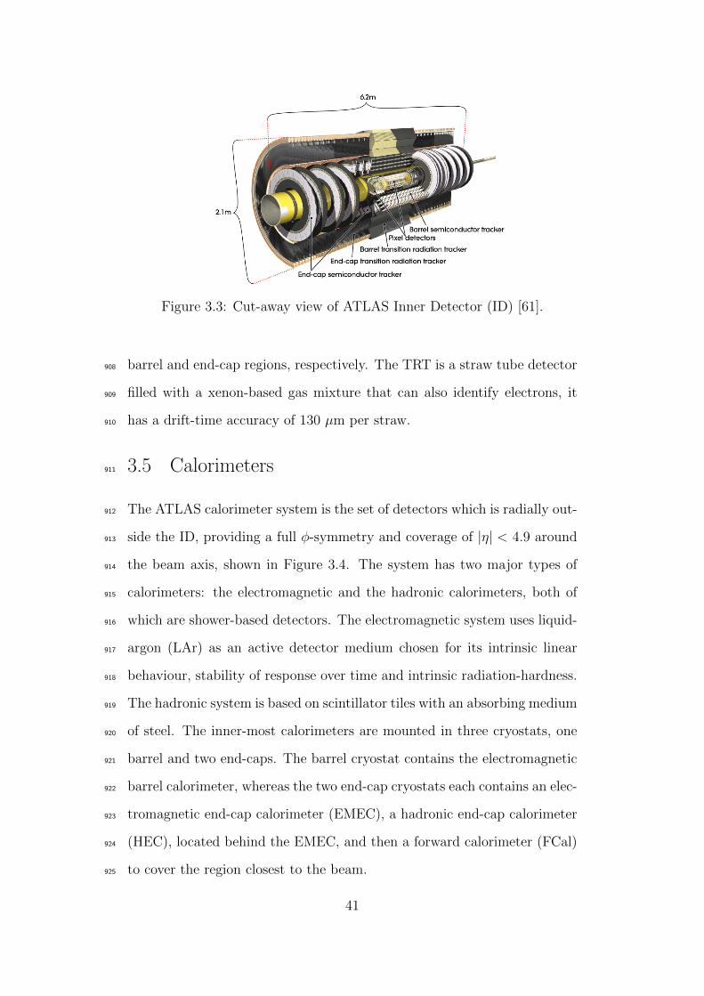
Figure 3.3: Cut-away view of ATLAS Inner Detector (ID) [61].
barrel and end-cap regions, respectively. The TRT is a straw tube detector908
filled with a xenon-based gas mixture that can also identify electrons, it909
has a drift-time accuracy of 130 µm per straw.910
3.5 Calorimeters911
The ATLAS calorimeter system is the set of detectors which is radially out-912
side the ID, providing a full φ-symmetry and coverage of |η| < 4.9 around913
the beam axis, shown in Figure 3.4. The system has two major types of914
calorimeters: the electromagnetic and the hadronic calorimeters, both of915
which are shower-based detectors. The electromagnetic system uses liquid-916
argon (LAr) as an active detector medium chosen for its intrinsic linear917
behaviour, stability of response over time and intrinsic radiation-hardness.918
The hadronic system is based on scintillator tiles with an absorbing medium919
of steel. The inner-most calorimeters are mounted in three cryostats, one920
barrel and two end-caps. The barrel cryostat contains the electromagnetic921
barrel calorimeter, whereas the two end-cap cryostats each contains an elec-922
tromagnetic end-cap calorimeter (EMEC), a hadronic end-cap calorimeter923
(HEC), located behind the EMEC, and then a forward calorimeter (FCal)924
to cover the region closest to the beam.925
41

Figure 3.4: The ATLAS calorimeters [61].
3.5.1 Liquid Argon Calorimeter926
The electromagnetic calorimeter mainly measures the energies of charged927
and neutral particles that interact electromagnetically, for example elec-928
trons and photons. It consists of several layers of accordion-shaped ab-929
sorbers of lead and copper electrodes, and LAr between them. For example,930
a high energy electron interacts with the absorber and forms a shower of931
low energy electrons, positrons and photons, which passes through LAr and932
produces more negatively charged electrons and positively charged ions by933
ionisation. Finally, these ionisation electrons are collected on electrodes934
and the charge is measured leading to measure energy of the primary935
electron. The accordion geometry of the LAr calorimeter provides sev-936
eral active layers in the system, three in the precision-measurement region937
(1.5 < |η| < 2.5), two in the higher-η region (2.5 < |η| < 3.2) and two in938
the overlap region (1.375 < |η| < 1.5) between the barrel and the EMEC.939
For |η| < 2.5, one of the high precision-measurement components with its940
three layers is shown in Figure 3.5, the first layer contains narrow strips941
positioned with a 4 mm separation in the η-direction with a very fine gran-942
ularity of ∆η × ∆φ = 0.0025 × 0.01. The second layer consists of small943
42

Figure 3.5: Drawing of barrel module of the LAr calorimeter [61].
segments placed into towers with granularity of ∆η×∆φ = 0.025 × 0.025.944
The third layer has relatively low precision, as compared to the previous945
two, with a granularity ∆η×∆φ = 0.05× 0.025. Overall, the barrel part of946
LAr calorimeter provides a coverage of |η| < 1.475, while the two end-cap947
components provide 1.375 < |η| < 3.2 coverage.948
3.5.2 Hadronic Calorimeter949
The tile calorimeter is the next layer to the electromagnetic calorimeter in950
both the barrel (|η| < 1) and the end cap regions (0.8 < |η| < 1.8). The951
hadronic system also works like the electromagnetic system. In this case,952
strongly interacting particles interact with the absorbing steel to produce953
showers of secondary hadrons (for example protons, neutrons and pions)954
and these showers interact with the scintillating tile material to produce955
the measurable signals.956
43

The HEC calorimeters are mounted in two wheels per end cap and957
placed just after the EMEC calorimeter. Each HEC wheel contains two958
layers and hence there are four HEC layers per end-cap. They cover the959
1.5 < |η| < 3.2 region with variable granularity: ∆η×∆φ = 0.1 × 0.1 for960
1.5 < |η| < 2.5 and 0.2 × 0.2 for the 2.5 < |η| < 3.2 region.961
The FCal provides higher electromagnetic and hadronic coverage in962
the forward region (3.1 < |η| < 4.9), mounted in each end-cap. It consists963
of three modules, also containing LAr as a sensitive material. The first964
one is made up of copper (to optimise electromagnetic interactions), while965
other two are made up of tungsten (to optimise hadronic interactions).966
3.6 Muon Spectrometers967
The outermost part of ATLAS detector is the muon spectrometer, designed968
to detect muons in the pseudorapidity range |η| < 2.7. The different compo-969
nents of Muon Spectrometer are shown in Figure 3.6. Energetic muons are970
typically the only detectable particles that can traverse all the calorimeters971
without being stopped. The muon spectrometer surrounds the calorime-972
ter and measures the muon’s path by determining their momenta with a973
typical resolution of about 10%. It contains thousands of charged particle974
sensors in the central and end-cap regions in order to perform a precision975
measurement. The sensors are similar to the straw tubes of the ID, but976
with larger tube diameters. The large superconducting toroidal coils inside977
the muon spectrometer produce a magnetic field of 0.5 T in the central978
region and 1 T in the end-caps regions. The minimum energy for muons to979
reach the spectrometer is ∼ 3 GeV, due to energy loss in the calorimeters.980
The precise tracking of muons through the spectrometer is accom-981
plished by CSCs (Cathode Strip Chambers) and MDT (Monitored Drift982
Tube) chambers. The fast trigger system of the spectrometer consists of983
44

three RPC (Resistive Plate Chamber) stations in the barrel, and three984
stations of TGCs (Thin Gap Chambers) in the end-cap regions.985
The MDT chambers consist of aluminium tubes with a central W -Re986
wire and a gas mixture of Ar-CO2, which is filled at an absolute pressure of987
3 bars that provides a maximum drift time of approximately 700 ns. The988
MDT chambers are constructed from 2 × 4 and 2 × 3 monolayers of drift989
tubes for the inner and middle/outer stations, respectively. In the drift990
chambers, the avalanche of secondary ionisations is being detected, which991
is proportional to the initial ionisation. The CSCs (2 < |η| < 2.7), using992
a mixture of Ar, CO2 and CF4 gas, are multiwire proportional chambers993
with a segmented cathode strip readout providing position measurements994
from the avalanche formed on the anode wire. The RPC (|η| < 1.05)995
is a gaseous detector (C2H2F4 gas), constructed without wires from two996
detector layers and four readout strip panels. It typically provides space997
and time resolutions of 1 cm and 1 ns, respectively. Finally, the TGCs998
(1.05 < |η| < 2.4) are multi-wire proportional chambers. The anode wires999
and readout strips of these chambers are arranged parallel and orthogonal,1000
respectively, to the MDT wires and provide both the spatial and trigger1001
information.1002
3.7 Forward Detectors1003
In addition to the main ATLAS detector systems described in previous1004
sections, there are five smaller sets of detectors to cover the forward region1005
in more detail: the Beam Condition Monitor (BCM), the Minimum Bias1006
Trigger Scintillator (MBTS), the LUminosity measurement using Cerenkov1007
Integrating Detector (LUCID), the Zero Degree Calorimeter (ZDC) and1008
the Absolute Luminosity ALFA detectors at distances 1.84 m, 3.6 m, 17 m,1009
140 m and 240 m from the IP of ATLAS, respectively. They are symmetric1010
45

Figure 3.6: Layout of Muon Spectrometer [63].
Forward Detectors Rapidity RangeBCM |η| ∼ 4.2MBTS 2.1 < |η| < 3.8LUCID 5.6 < |η| < 5.9ZDC |η| > 8.3ALFA 1.06 < |η| < 13.5
Table 3.1: Rapidities of forward detectors of ATLAS.
on either side of the IP. Along with the central detectors of ATLAS, the1011
forward detectors provide an additional rapidity coverage in the forward1012
regions as shown in Table 3.1. The forward detectors are closely connected1013
to the luminosity determination in ATLAS, which will briefly be described1014
in the next section.1015
3.8 Luminosity Measurement1016
The ATLAS luminosity is measured in inelastic interactions by using dif-1017
ferent forward detectors and their corresponding counting-algorithms [64].1018
For a given fraction of bunch crossings (BXs), the number of registered1019
events by a detector are counted according to specific selection criteria,1020
with event selection efficiency (ε), which depends on the specific detector1021
46

and the algorithm chosen. The luminosity (L) corresponding to an inelastic1022
cross section (σinel), for the total number of BXs at the IP (nb) and the1023
number of inelastic interactions per BX (µ), can be written as1024
L =µnbfrσinel
=µvisnbfrσvis
, (3.1)
where fr is the bunch revolution frequency of the proton bunches. In the1025
above equation, σvis is the visible cross section related to the average visible1026
interactions per BX (µvis). The quantity µvis is the visible quantity seen1027
by a detector which is defined as µvis ≡ εµ, hence σvis ≡ εσinel. In the1028
limit µvis � 1, i.e., for a low number of interactions per BX, µvis is linearly1029
related to the event counting in a detector (N vis) as1030
σvis ≈N vis
NBX
(3.2)
where NBX are the number of bunch crossings in the same time interval in1031
which N vis are measured. On the other hand, when µ increases, the prob-1032
ability of two or more than two pp interactions in the same BX is no longer1033
negligible, and the relation between µvis and N vis is not linear anymore.1034
Therefore, for high µvis, Poisson statistics must be taken into account. The1035
detector algorithms are modified to take the Poisson distribution effects1036
into account for the luminosity calculations.1037
There is another method for luminosity measurement which neither1038
requires any prior knowledge of cross section nor depends on detector effi-1039
ciencies. It is known as the van der Meer (vdM) scans method [65]. This1040
technique only depends on the machine parameters and luminosity. The1041
equation for the vdM scans method is written as1042
L =nbfrn1n2
2πΣxΣy
, (3.3)
where n1 and n2 are the number of protons in two colliding bunches, and Σx1043
and Σy are the numbers measured from the horizontal and vertical beam1044
47

profiles scanned by vdM method. However, this method requires some1045
dedicated runs and special setup to scan the beam profiles.1046
3.9 Triggers and Data Acquisition1047
The ATLAS trigger and data acquisition system is a three level online1048
data refinery, and events which pass all the three levels are written out for1049
the offline analysis. The Level-1 (L1) trigger takes information from sub1050
detectors, reduces the event rate to about 75 kHz, and makes an initial1051
selection. For example, it recognises muon pT from the RPCs and TGCs,1052
and accepts electrons, hadrons and jets from the calorimeter system. The1053
latency of L1 is the time between pp collisions and the time at which the1054
decision of L1 is available for the next level, Level-2 (L2), which is 2.5 µs.1055
Therefore, in this small time L1 decides whether to send this information1056
to L2 or not.1057
The selection criteria of L2 trigger are based on the information1058
provided by L1, called Regions-of-Interest (RoIs). A RoI information can1059
include various parameters such as pT , missing transverse energy EmissT , and1060
the positions of particles in (η,φ). Along with the L1-RoI, the L2 trigger1061
uses some additional RoIs with some tighter cuts to process an event in less1062
than 40 ms, and reduces the trigger rate to ∼ 3.5 kHz. The Event Filter1063
(EF) is the last stage of the online trigger system, which also uses RoI. The1064
EF reduces the event rate to 200 Hz and processes an event on the order of1065
1 s, and therefore has an ability to run a complex analysis on the data due1066
to the longer processing time available. The EF is able to filter events with1067
respect to different physics needs, for example events with high pT jets are1068
used for this analysis. Finally, these events are written out to mass storage1069
for offline analysis.1070
48

Chapter 41071
Analysis1072
In this chapter, the search for microscopic black holes in multijet final states1073
for pp collisions with 8 TeV centre of mass energy at the LHC, using the1074
ATLAS 2012 data, is presented. The study is mainly data-driven, but uses1075
corrections derived from MC-simulations (MCs) of QCD. The black hole1076
search in this analysis is based on low-scale gravity models which predict1077
production of non-perturbative gravitational states, such as black holes in1078
high energy particle collisions at the LHC [66].1079
4.1 Introduction1080
According to low-scale gravity models, the hierarchy problem (described in1081
chapter 1) can be solved when the fundamental gravitational scale reduces1082
to the order of the electroweak scale. As a consequence, the production1083
of black holes or string balls may occur at the LHC with masses much1084
higher than the fundamental gravitational scale. Once produced, the mi-1085
croscopic black holes at the LHC will act like classical thermal states and1086
quickly decay to a large number of particles (high multiplicity) with high1087
pT . As discussed in sbusection 2.4.4 and section 2.5 that the black hole1088
decay mainly leads to the production of jets of hadrons in the detector.1089
Therefore, high pT multijet final states are chosen as a potential signal for1090
the microscopic black holes.1091
49

In this study, we look for high multiplicity multijet final states with1092
high pT . The suitable variable is the scalar sum of jet-pT (HT =∑pT ).1093
For different jet multiplicity bins, the shape of the HT distribution is ex-1094
pected to be the same because initial state radiation (ISR) and final state1095
radiation (FSR) are collinear in nature with respect to the incoming and1096
outgoing partons. The assumption of the HT shape invariance for the1097
QCD-type events allows us to predict the QCD background for all the jet1098
multiplicities. Since microscopic black holes are expected to decay to high1099
jet multiplicities, the lowest multiplicity case of dijet is therefore chosen as1100
the control region. The most invariant sub-region of HT with multiplicity1101
of the control region is defined as the normalisation region in the HT dis-1102
tribution for all the jet multiplicities, where there are no black holes seen.1103
By using the shape invariance assumption and a fit-based technique, the1104
control region fits, along with the appropriate normalisation factors, are1105
applied to jet multiplicities larger than two in order to estimate the back-1106
ground in the signal region. By considering all the possible uncertainties1107
in the signal region, model-independent and model-dependent upper limits1108
are derived for the inclusive jet multiplicities N ≥ 3, 4, ..., 7. This analysis1109
method is adopted from the previous studies for microscopic black hole1110
searches in the ATLAS [67] and CMS [7–10] collaborations.1111
4.2 Monte Carlo Simulations1112
QCD multijet events constitute the dominant background in the search1113
region. PYTHIA8 [68] and HERWIG++ [69] dijet MC samples are used1114
to study the main background. All other background contributions from1115
events such as tt, Z+jets, W+jets, di-boson (ZZ, WW, WZ) and γ+jets1116
are considerably small and can be ignored [7, 8, 10]. Detailed descriptions1117
of generated dijet samples will be illustrated in next subsection.1118
50

All the MC samples are passed through a full simulation of the1119
ATLAS detector [70] using GEANT4 [71]. All the MC simulated data1120
samples used in this analysis have been produced centrally by the ATLAS1121
collaboration for 8 TeV centre of mass energy in order to compare with the1122
ATLAS 2012 data. The MC simulated data is also corrected with respect1123
to pileup effects (described in Appendix E) in the 2012 data. Finally, the1124
MC events are reconstructed and analyzed with the same procedures as1125
used on the data.1126
4.2.1 QCD Background Samples1127
The baseline simulated QCD MC samples are generated using PYTHIA81128
implementing leading-order (LO) perturbative QCD matrix elements for1129
2→ 2 processes and pT -ordered parton showers calculated in a leading log-1130
arithmic approximation with the ATLAS AU2 tune [72] and the CT10 PDF1131
set [73]. Effectively, these samples are generated for eight different leading1132
jet pT regions based on their cross sections covering the entire pT spectrum1133
accessible by the ATLAS detector. The PYTHIA8 MC samples produced1134
for different leading jet pT slices are named as JZ0W,JZ1W, ..., JZ7W ,1135
and also called J-samples. At the generator level, events are filtered by the1136
pT cut corresponding to each J-sample. The efficiency of this cut is known1137
as the filter efficiency. The dataset identifiers (DSIDs), number of events,1138
pT ranges, cross sections and the filter efficiencies for all the J-samples are1139
given in Table 4.1.1140
Similarly, HERWIG++ [69] is used to produce another type of base-1141
line QCD events for 2 → 2 processes with the EE3 tune [74] and the1142
CTEQ6L1 PDF set [75]. Different slices with corresponding DSIDs based1143
on their cross sections and filter efficiencies are shown in Table 4.2. All the1144
specifications of both the QCD MC events are also compared in Table 4.3.1145
51

DSID Slice Events pT [TeV] Cross section [fb] Filter Efficiency
147910 JZ0W 1500000 0-0.02 7.3 × 10¹³ 9.9 × 10⁻¹
147911 JZ1W 1599994 0.02-0.08 7.3 × 10¹³ 1.3 × 10⁻⁴
147912 JZ2W 5999034 0.08-0.2 2.6 × 10¹⁰ 4.0 × 10⁻³
147913 JZ3W 5977254 0.2-0.5 5.4 × 10⁸ 1.2 × 10⁻³
147914 JZ4W 5997214 0.5-1.0 6.4 × 10⁶ 7.1 × 10⁻⁴
147915 JZ5W 2996082 1.0-1.5 4.0 × 10⁴ 2.2 × 10⁻³
147916 JZ6W 2993651 1.5-2.0 4.2 × 10² 4.7 × 10⁻⁴
147917 JZ7W 2991955 >2.0 4.1 × 101 1.5 × 10⁻²
Table 4.1: PYTHIA8 dijet MC weighted samples with their correspondingdataset identifier (DSID), name of the sample (Slice), number of events,pT range, cross section and the efficiency of the kinematic filter at thegenerator level (Filter Efficiency) are shown.
For both the PYTHIA8 and HERWIG++ MCs, all the J-samples (pT1146
slices) need to be properly weighted and combined together in order to1147
obtain the whole pT spectrum. A J-sample can be weighted corresponding1148
to its filter efficiency εF , cross section σ, weight of each event and the total1149
number of events as following1150
Weight =εF × σ × Event weight
Number of events. (4.1)
The above pT slice weight is applied on an event by event basis for each1151
J-sample. Finally, all the weighted samples are combined to obtain a full1152
pT distribution in order to compare it with the data distribution.1153
4.3 Trigger1154
The selection of a trigger is the starting point of an analysis, as it decides1155
whether to reject an event or keep it for the analysis. Different types of trig-1156
gers are designed based on objects (electrons, photons, muons, jets, etc.)1157
and physics needs. Since HT is the key variable of this analysis, and micro-1158
scopic black hole signals are expected to lie in the high HT region, a trigger1159
requiring high pT jets and high HT would be suitable for this analysis. The1160
52

DSID Slice Events Cross section [fb] Filter Efficiency
159110 JZ0W 1399998 1.2 × 10⁸ 9.9 × 10⁻¹
159111 JZ1W 1399897 3.6 × 10¹² 1.4 × 10⁻³
159112 JZ2W 1399993 1.9 × 10¹⁰ 2.6 × 10⁻³
159113 JZ3W 1399680 3.6 × 10⁸ 8.5 × 10⁻⁴
159114 JZ4W 1399665 4.2 × 10⁶ 5.4 × 10⁻⁴
159115 JZ5W 399490 8.3 × 10⁴ 5.5 × 10⁻⁴
159116 JZ6W 1389845 5.8 × 10³ 2.0 × 10⁻⁴
159117 JZ7W 1396932 6.5 × 10² 5.7 × 10⁻⁴
Table 4.2: HERWIG++ dijet MC weighted samples with their correspondingdataset identifier (DSID), name of the sample (Slice), number of events,cross section and the efficiency of the kinematic filter at the generator level(Filter Efficiency) are shown.
Generator PYTHIA8 HERWIG++
Process dijet dijetMatrix PYTHIA8 HERWIG++
Hadronisation PYTHIA8 HERWIG++
Underlying Event PYTHIA8 HERWIG++
ATLAS Tune AU2 EE3PDF Set CT10 CETQ6L1
Table 4.3: Matrix element generator, hadronisation generator, underlyingevent generator, ATLAS tune and parton distribution function (PDF) setis shown for both PYTHIA8 and HERWIG++ QCD dijet MC events.
53

EF j170 a4tchad ht700 trigger fulfills the need of this study by requiring at1161
least one reconstructed hadronic jet of pT ≥ 170 GeV and HT ≥ 700 GeV1162
at the EF level. The term a4tchad stands for a hadronic (had) jet, which1163
is reconstructed from topological clusters (tc) [76] of calorimeters by using1164
an anti-kt algorithm [77] with a distance parameter R = 0.4 (a4) [77, 78].1165
The trigger efficiency has been studied as a function of the leading jet pT1166
and HT with respect to the reference trigger EF j110 a4tchad. If the main1167
trigger EF j170 a4tchad ht700 and the reference trigger EF j110 a4tchad1168
are represented as “A” and “B”, respectively, then the trigger efficiency for1169
a variable is calculated as1170
Trigger Efficiency =A ∩BB
. (4.2)
The trigger efficiency as a function of the leading jet pT and HT is shown1171
in Figure 4.1. The correlation between the two variables shows that the1172
fully efficient region of the trigger can be obtained for HT > 0.9 TeV.1173
Furthermore, the trigger efficiency as a function of the leading jet pT and1174
HT is shown independent of each other in Figure 4.2, which confirms the HT1175
threshold for the plateau region. Further details on the trigger efficiency1176
are shown in Appendix B.1177
4.4 Data Selection1178
The analysis is performed over the full 2012 data set of pp collisions at1179
√s = 8 TeV collected by the ATLAS detector, corresponding to an in-1180
tegrated luminosity of 20.3 fb−1. The data for the year are divided into1181
different data periods, e.g., period-A, period-B, and so on, corresponding1182
to certain time spans of data-taking. A data period consists of the data1183
runs which are made according to the stability of beam conditions at the1184
LHC and detectors collecting the data. A run is further divided into lumi-1185
blocks tagged with numbers called lumi-block numbers (lbn). The length1186
54

0.0
0.1
0.2
0.3
0.4
0.5
0.6
0.7
0.8
0.9
1.0
[TeV]T
H
0.0 0.2 0.4 0.6 0.8 1.0 1.2 1.4 1.6 1.8 2.0
[T
eV
]T
Le
ad
ing
je
t p
0.05
0.10
0.15
0.20
0.25
0.30
0.35
0.40
0.45
0.50
EF_j170_a4tchad_ht700
Reference, EF_j110_a4tchad1
Ldt = 20.3 fb∫ = 8 TeV, s
Figure 4.1: The EF j170 a4tchad ht700 trigger efficiency versus leading jetpT and HT , with respect to the reference EF j110 a4tchad trigger.
of each lumi-block is on the order of a few minutes and contains several1187
data events. The reason for dividing the data into runs and lumi-blocks is1188
to create a computing ease to deal with the problematic parts of the data1189
with respect to their time stamps while doing the offline analysis. These1190
affected data may arise because of several factors while data-taking. For1191
example, hardware issues in detectors because of the intense radiation envi-1192
ronment or any other reason like electronic noise, non-collision and cosmic1193
ray background, etc. can be sources of bad data collected during collisions.1194
In order to discard the bad data, different physics groups in the ATLAS1195
collaboration define good run lists according to their analysis requirements.1196
The data is then stored in different formats for offline analyses. The1197
ATLAS physics groups make their own short formatted data sets by filtering1198
the raw data according to their physics needs. Furthermore, the data events1199
are filtered using standard event cleaning criteria.1200
55

[TeV]T
Leading jet p0.0 0.2 0.4 0.6 0.8 1.0 1.2 1.4
Trig
ge
r E
ffic
ien
cy
0.0
0.2
0.4
0.6
0.8
1.0
EF_j170_a4tchad_ht700
Reference, EF_j110_a4tchad1
Ldt = 20.3 fb∫ = 8 TeV, s
(a) The trigger efficiency as a function of the leading jet pT .
[TeV]T
H0.0 0.2 0.4 0.6 0.8 1.0 1.2 1.4 1.6 1.8 2.0
Trig
ge
r E
ffic
ien
cy
0.0
0.2
0.4
0.6
0.8
1.0
EF_j170_a4tchad_ht700
Reference, EF_j110_a4tchad1
Ldt = 20.3 fb∫ = 8 TeV, s
(b) The trigger efficiency as a function of the HT .
Figure 4.2: The EF j170 a4tchad ht700 trigger efficiency with respect tothe reference trigger EF j110 a4tchad.
56

4.4.1 Event Selection1201
All the good runs and lumi-blocks for the ATLAS 2012 data are used.1202
Events are required to have a reconstructed primary vertex associated with1203
at least two tracks. The data events are only considered when the trigger1204
system, tracking detectors, calorimeters and magnets were operating at1205
the nominal conditions. More details on event selection can be found in1206
Appendix C.1207
4.4.2 Jet Selection1208
This study is mainly focused on multijet final states. Well-reconstructed1209
hadronic jets, along with the jets which are made due to photons and1210
electrons, are used. Since microscopic black holes are expected to decay1211
predominately to SM particles. By considering multijet final states most1212
of the potential black hole signatures are taken into account. Moreover,1213
since the jets from electrons and photons are not identified as different1214
objects than the hadronic jets there is no concern for object double count-1215
ing. Therefore, this multijet analysis that does not identify other objects1216
considerably simplifies the search method.1217
In the ATLAS data, jets are reconstructed using the anti-kt clus-1218
tering algorithm with different values of jet distance parameter [77, 78].1219
Anti-kt jets with a distance parameter R = 0.4 made up of topological1220
calorimeter clusters with a positive energy are used. Furthermore, local1221
cluster weighting (LCW) calibration is used for the jets, which can distin-1222
guish between electromagnetic and hadronic jets to apply the appropriate1223
corrections accordingly, greatly improving the jet energy resolution. The1224
jet pT measurement is further improved by applying offline calibrations and1225
corrections based on different factors such as pseudorapidity, transverse en-1226
ergy and momentum, event topology and event pileup effects [79]. All good1227
57

jets (shown in appendix C.1.4), defined by the percentage of tracks in the jet1228
originating from the vertex, are used. Furthermore, jets with pT > 50 GeV1229
are selected to minimize pileup effects. The detailed description of the event1230
pileup and choice of pT > 50 GeV is mentioned in appendix E. In order to1231
obtain the well-measured jets, only jets reconstructed in the central region1232
of the ATLAS detector, i.e. |η| < 2.8, are chosen.1233
For different jet multiplicities (N = 2, 3, ..., 7) the jet pT and η1234
distributions are shown in Figures 4.3 and 4.4, respectively. Both the pT and1235
η distributions for the ATLAS 2012 data are compared with PYTHIA8 and1236
HERWIG++ MCs. For a given jet multiplicity, the dijet MC distributions1237
are normalized with respect to the area under the data curve. For the1238
jet pT , both PYTHIA8 and HERWIG++ MCs agree with the data to within1239
30% and are also in good agreement to each other. However, for the jet1240
η, from the data to MC ratio at the bottom of each plot in Figure 4.4,1241
the agreement of the data with PYTHIA8 MC is better than the data with1242
HERWIG++ MC.1243
4.5 Data Characteristics1244
HT is the main variable of this analysis, constructed from the scalar sum1245
of pT of jets with pT > 50 GeV and pseudorapidity |η| < 2.8, summarized1246
as1247
HT =∑
pT for pT > 50 GeV and |η| < 2.8. (4.3)
The HT variable is directly formed from the jet pT which have good agree-1248
ment between the data and the MCs, as shown in Figure 4.3. Therefore,1249
the disagreement of the data and MCs for the η distributions, shown in1250
Figure 4.4, does not affect the analysis strategy. Furthermore, some other1251
jet kinematic variables, the leading jet pT , the second leading jet pT and1252
the jet φ, are shown in appendix D.1253
58

0.0 0.5 1.0 1.5 2.0 2.5
Entr
ies / 0
.1 T
eV
1
10
210
310
410
510
610
710
1
Ldt = 20.3 fb∫ = 8 TeV, s
| < 2.8η > 50 GeV, |T
Jets, p
Multiplicity, N = 2
Data
Pythia8 dijet
Herwig++ dijet
Data / Pythia8
Data / Herwig++
[TeV]T
p0.0 0.5 1.0 1.5 2.0 2.5
Da
ta /
MC
0.60.81.01.21.41.6 0.0 0.5 1.0 1.5 2.0 2.5
Entr
ies / 0
.1 T
eV
1
10
210
310
410
510
610
710
1
Ldt = 20.3 fb∫ = 8 TeV, s
| < 2.8η > 50 GeV, |T
Jets, p
Multiplicity, N = 3
Data
Pythia8 dijet
Herwig++ dijet
Data / Pythia8
Data / Herwig++
[TeV]T
p0.0 0.5 1.0 1.5 2.0 2.5
Da
ta /
MC
0.60.81.01.21.41.6
0.0 0.5 1.0 1.5 2.0 2.5
Entr
ies / 0
.1 T
eV
1
10
210
310
410
510
610
710
1
Ldt = 20.3 fb∫ = 8 TeV, s
| < 2.8η > 50 GeV, |T
Jets, p
Multiplicity, N = 4
Data
Pythia8 dijet
Herwig++ dijet
Data / Pythia8
Data / Herwig++
[TeV]T
p0.0 0.5 1.0 1.5 2.0 2.5
Da
ta /
MC
0.60.81.01.21.41.6 0.0 0.5 1.0 1.5 2.0 2.5
Entr
ies / 0
.1 T
eV
1
10
210
310
410
510
610
710
1
Ldt = 20.3 fb∫ = 8 TeV, s
| < 2.8η > 50 GeV, |T
Jets, p
Multiplicity, N = 5
Data
Pythia8 dijet
Herwig++ dijet
Data / Pythia8
Data / Herwig++
[TeV]T
p0.0 0.5 1.0 1.5 2.0 2.5
Da
ta /
MC
0.60.81.01.21.41.6
0.0 0.5 1.0 1.5 2.0 2.5
Entr
ies / 0
.1 T
eV
1
10
210
310
410
510
610
710
1
Ldt = 20.3 fb∫ = 8 TeV, s
| < 2.8η > 50 GeV, |T
Jets, p
Multiplicity, N = 6
Data
Pythia8 dijet
Herwig++ dijet
Data / Pythia8
Data / Herwig++
[TeV]T
p0.0 0.5 1.0 1.5 2.0 2.5
Da
ta /
MC
0.60.81.01.21.41.6 0.0 0.5 1.0 1.5 2.0 2.5
Entr
ies / 0
.1 T
eV
1
10
210
310
410
510
610
710
1
Ldt = 20.3 fb∫ = 8 TeV, s
| < 2.8η > 50 GeV, |T
Jets, p
Multiplicity, N = 7
Data
Pythia8 dijet
Herwig++ dijet
Data / Pythia8
Data / Herwig++
[TeV]T
p0.0 0.5 1.0 1.5 2.0 2.5
Da
ta /
MC
0.60.81.01.21.41.6
Figure 4.3: The jet pT distributions for the exclusive jet multiplicities,N = 2, 3, ..., 7, for the ATLAS 2012 data, PYTHIA8 (red) and HERWIG++
(blue) MCs. At the bottom of each plot, the ratio of the data to the MCare shown for both the MCs.
59

3 2 1 0 1 2 3
Entr
ies / 0
.1 T
eV
1
10
210
310
410
510
610
710
810
910
1
Ldt = 20.3 fb∫ = 8 TeV, s
| < 2.8η > 50 GeV, |T
Jets, p
Multiplicity, N = 2
Data
Pythia8 dijet
Herwig++ dijet
Data / Pythia8
Data / Herwig++
η3 2 1 0 1 2 3
Da
ta /
MC
0.70.80.91.01.11.21.3 3 2 1 0 1 2 3
Entr
ies / 0
.1 T
eV
1
10
210
310
410
510
610
710
810
910
1
Ldt = 20.3 fb∫ = 8 TeV, s
| < 2.8η > 50 GeV, |T
Jets, p
Multiplicity, N = 3
Data
Pythia8 dijet
Herwig++ dijet
Data / Pythia8
Data / Herwig++
η3 2 1 0 1 2 3
Da
ta /
MC
0.70.80.91.01.11.21.3
3 2 1 0 1 2 3
Entr
ies / 0
.1 T
eV
1
10
210
310
410
510
610
710
810
910
1
Ldt = 20.3 fb∫ = 8 TeV, s
| < 2.8η > 50 GeV, |T
Jets, p
Multiplicity, N = 4
Data
Pythia8 dijet
Herwig++ dijet
Data / Pythia8
Data / Herwig++
η3 2 1 0 1 2 3
Da
ta /
MC
0.70.80.91.01.11.21.3 3 2 1 0 1 2 3
Entr
ies / 0
.1 T
eV
1
10
210
310
410
510
610
710
810
910
1
Ldt = 20.3 fb∫ = 8 TeV, s
| < 2.8η > 50 GeV, |T
Jets, p
Multiplicity, N = 5
Data
Pythia8 dijet
Herwig++ dijet
Data / Pythia8
Data / Herwig++
η3 2 1 0 1 2 3
Da
ta /
MC
0.70.80.91.01.11.21.3
3 2 1 0 1 2 3
Entr
ies / 0
.1 T
eV
1
10
210
310
410
510
610
710
810
910
1
Ldt = 20.3 fb∫ = 8 TeV, s
| < 2.8η > 50 GeV, |T
Jets, p
Multiplicity, N = 6
Data
Pythia8 dijet
Herwig++ dijet
Data / Pythia8
Data / Herwig++
η3 2 1 0 1 2 3
Da
ta /
MC
0.70.80.91.01.11.21.3 3 2 1 0 1 2 3
Entr
ies / 0
.1 T
eV
1
10
210
310
410
510
610
710
810
910
1
Ldt = 20.3 fb∫ = 8 TeV, s
| < 2.8η > 50 GeV, |T
Jets, p
Multiplicity, N = 7
Data
Pythia8 dijet
Herwig++ dijet
Data / Pythia8
Data / Herwig++
η3 2 1 0 1 2 3
Da
ta /
MC
0.70.80.91.01.11.21.3
Figure 4.4: The η distributions of jets for the exclusive jet multiplicities,N = 2, 3, ..., 7, for the ATLAS 2012 data, PYTHIA8 (red) and HERWIG++
(blue) MCs. At the bottom of each plot, the ratio of the data to the MCare shown for both the MCs.
60

4.5.1 The HT Distributions1254
In this multijet analysis searching for microscopic black hole, the HT dis-1255
tributions play an important role. The comparison of the HT distributions1256
for the ATLAS 2012 data, PYTHIA8 and HERWIG++ MCs has been shown1257
in Figures 4.5 and 4.6 for the exclusive jet multiplicities, N = 2, 3, .., 7, and1258
inclusive jet multiplicities, N ≥ 2, 3, ..., 7, respectively. From Figure 4.5,1259
for the exclusive jet multiplicities, the data and the MCs are within 20%1260
agreement, similar to the pT distributions (Figure 4.3), whereas the agree-1261
ment is improved for the inclusive jet multiplicities, as shown in Figure 4.6.1262
Since for the inclusive jet multiplicities, many jet multiplicities are consid-1263
ered at once with a lower threshold on jet multiplicity, e.g., N ≥ 3. The1264
disagreements are therefore compensated to an extent in the HT distribu-1265
tions.1266
The shapes of the HT distributions are expected to be the same for1267
all types of multijet final states and this is the key assumption to estimate1268
the major QCD background in this study. The shape invariance of the1269
HT distributions for different jet multiplicities, both for the inclusive and1270
exclusive multiplicity cases, will be examined in the next subsection.1271
4.5.2 Shape Invariance of Kinematic Distributions1272
The shape of the HT distribution is considered to be invariant with the jet1273
multiplicity. The shape invariance is expected above an HT value set by the1274
jet pT > 0.05 TeV selection, i.e., HT > [N × 0.05] TeV. The multiplicity-1275
dependent onset for invariance can be observed if the HT ratios of mul-1276
tiplicities N > 2 are inspected with respect to the case of two jets, i.e.1277
N = 2, as shown in Figures 4.7 and 4.8. The reason of choosing dijet case1278
as a benchmark case will be described at the end of this subsection. The1279
onset for invariance is different for different multiplicities, but to keep the1280
61
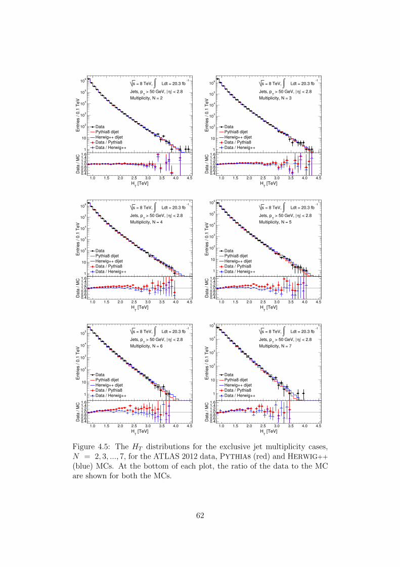
1.0 1.5 2.0 2.5 3.0 3.5 4.0 4.5
Entr
ies / 0
.1 T
eV
1
10
210
310
410
510
610 1
Ldt = 20.3 fb∫ = 8 TeV, s
| < 2.8η > 50 GeV, |T
Jets, p
Multiplicity, N = 2
DataPythia8 dijet
Herwig++ dijetData / Pythia8
Data / Herwig++
[TeV]T
H
1.0 1.5 2.0 2.5 3.0 3.5 4.0 4.5
Da
ta /
MC
0.40.60.81.01.21.41.6 1.0 1.5 2.0 2.5 3.0 3.5 4.0 4.5
Entr
ies / 0
.1 T
eV
1
10
210
310
410
510
610
1
Ldt = 20.3 fb∫ = 8 TeV, s
| < 2.8η > 50 GeV, |T
Jets, p
Multiplicity, N = 3
DataPythia8 dijet
Herwig++ dijetData / Pythia8
Data / Herwig++
[TeV]T
H
1.0 1.5 2.0 2.5 3.0 3.5 4.0 4.5
Da
ta /
MC
0.40.60.81.01.21.41.6
1.0 1.5 2.0 2.5 3.0 3.5 4.0 4.5
Entr
ies / 0
.1 T
eV
1
10
210
310
410
510
610
1
Ldt = 20.3 fb∫ = 8 TeV, s
| < 2.8η > 50 GeV, |T
Jets, p
Multiplicity, N = 4
DataPythia8 dijet
Herwig++ dijetData / Pythia8
Data / Herwig++
[TeV]T
H
1.0 1.5 2.0 2.5 3.0 3.5 4.0 4.5
Da
ta /
MC
0.40.60.81.01.21.41.6 1.0 1.5 2.0 2.5 3.0 3.5 4.0 4.5
Entr
ies / 0
.1 T
eV
1
10
210
310
410
510
610 1
Ldt = 20.3 fb∫ = 8 TeV, s
| < 2.8η > 50 GeV, |T
Jets, p
Multiplicity, N = 5
DataPythia8 dijet
Herwig++ dijetData / Pythia8
Data / Herwig++
[TeV]T
H
1.0 1.5 2.0 2.5 3.0 3.5 4.0 4.5
Da
ta /
MC
0.40.60.81.01.21.41.6
1.0 1.5 2.0 2.5 3.0 3.5 4.0 4.5
Entr
ies / 0
.1 T
eV
1
10
210
310
410
510
1
Ldt = 20.3 fb∫ = 8 TeV, s
| < 2.8η > 50 GeV, |T
Jets, p
Multiplicity, N = 6
DataPythia8 dijet
Herwig++ dijetData / Pythia8
Data / Herwig++
[TeV]T
H
1.0 1.5 2.0 2.5 3.0 3.5 4.0 4.5
Da
ta /
MC
0.40.60.81.01.21.41.6 1.0 1.5 2.0 2.5 3.0 3.5 4.0 4.5
Entr
ies / 0
.1 T
eV
1
10
210
310
410
510
1
Ldt = 20.3 fb∫ = 8 TeV, s
| < 2.8η > 50 GeV, |T
Jets, p
Multiplicity, N = 7
DataPythia8 dijet
Herwig++ dijetData / Pythia8
Data / Herwig++
[TeV]T
H
1.0 1.5 2.0 2.5 3.0 3.5 4.0 4.5
Da
ta /
MC
0.40.60.81.01.21.41.6
Figure 4.5: The HT distributions for the exclusive jet multiplicity cases,N = 2, 3, ..., 7, for the ATLAS 2012 data, PYTHIA8 (red) and HERWIG++
(blue) MCs. At the bottom of each plot, the ratio of the data to the MCare shown for both the MCs.
62

1.0 1.5 2.0 2.5 3.0 3.5 4.0 4.5
Entr
ies / 0
.1 T
eV
1
10
210
310
410
510
610
710
1
Ldt = 20.3 fb∫ = 8 TeV, s
| < 2.8η > 50 GeV, |T
Jets, p
2≥Multiplicity, N
DataPythia8 dijet
Herwig++ dijetData / Pythia8
Data / Herwig++
[TeV]T
H
1.0 1.5 2.0 2.5 3.0 3.5 4.0 4.5
Da
ta /
MC
0.40.60.81.01.21.41.6 1.0 1.5 2.0 2.5 3.0 3.5 4.0 4.5
Entr
ies / 0
.1 T
eV
1
10
210
310
410
510
610
710
1
Ldt = 20.3 fb∫ = 8 TeV, s
| < 2.8η > 50 GeV, |T
Jets, p
3≥Multiplicity, N
DataPythia8 dijet
Herwig++ dijetData / Pythia8
Data / Herwig++
[TeV]T
H
1.0 1.5 2.0 2.5 3.0 3.5 4.0 4.5
Da
ta /
MC
0.40.60.81.01.21.41.6
1.0 1.5 2.0 2.5 3.0 3.5 4.0 4.5
Entr
ies / 0
.1 T
eV
1
10
210
310
410
510
610
1
Ldt = 20.3 fb∫ = 8 TeV, s
| < 2.8η > 50 GeV, |T
Jets, p
4≥Multiplicity, N
DataPythia8 dijet
Herwig++ dijetData / Pythia8
Data / Herwig++
[TeV]T
H
1.0 1.5 2.0 2.5 3.0 3.5 4.0 4.5
Da
ta /
MC
0.40.60.81.01.21.41.6 1.0 1.5 2.0 2.5 3.0 3.5 4.0 4.5
Entr
ies / 0
.1 T
eV
1
10
210
310
410
510
610 1
Ldt = 20.3 fb∫ = 8 TeV, s
| < 2.8η > 50 GeV, |T
Jets, p
5≥Multiplicity, N
DataPythia8 dijet
Herwig++ dijetData / Pythia8
Data / Herwig++
[TeV]T
H
1.0 1.5 2.0 2.5 3.0 3.5 4.0 4.5
Da
ta /
MC
0.40.60.81.01.21.41.6
1.0 1.5 2.0 2.5 3.0 3.5 4.0 4.5
Entr
ies / 0
.1 T
eV
1
10
210
310
410
510
1
Ldt = 20.3 fb∫ = 8 TeV, s
| < 2.8η > 50 GeV, |T
Jets, p
6≥Multiplicity, N
DataPythia8 dijet
Herwig++ dijetData / Pythia8
Data / Herwig++
[TeV]T
H
1.0 1.5 2.0 2.5 3.0 3.5 4.0 4.5
Da
ta /
MC
0.40.60.81.01.21.41.6 1.0 1.5 2.0 2.5 3.0 3.5 4.0 4.5
Entr
ies / 0
.1 T
eV
1
10
210
310
410
510
1
Ldt = 20.3 fb∫ = 8 TeV, s
| < 2.8η > 50 GeV, |T
Jets, p
7≥Multiplicity, N
DataPythia8 dijet
Herwig++ dijetData / Pythia8
Data / Herwig++
[TeV]T
H
1.0 1.5 2.0 2.5 3.0 3.5 4.0 4.5
Da
ta /
MC
0.40.60.81.01.21.41.6
Figure 4.6: The HT distributions for the inclusive jet multiplicity cases,N ≥ 2, 3, ..., 7, for the ATLAS 2012 data, PYTHIA8 (red) and HERWIG++
(blue) MCs. At the bottom of each plot, the ratio of the data to the MCare shown for both the MCs.
63

background estimation procedure general, a common invariant region for1281
all the jet multiplicities is defined. From Figures 4.7 and 4.8, by consid-1282
ering all multiplicity cases under observation, the HT > 1.7 TeV region is1283
chosen where the plateau is observed in the ratio plots. By ignoring the1284
HT < 1.7 TeV region, some kinematical effects can be removed, but still1285
there are some non-invariance effects (negative slopes) for the HT > 1.7 TeV1286
region. These non-invariant effects can be minimized by applying correc-1287
tions which will be discussed later in this section. After choosing the lower1288
HT threshold, different upper thresholds on the HT ratios have been stud-1289
ied and the 1.7 < HT < 2.4 TeV region is chosen as the flattest region in1290
the HT ratios and is defined as the normalisation region.1291
In order to investigate the shape invariance of the HT distribution, a1292
detailed study is performed in the normalisation region based on the flatness1293
of the ratio of the HT distributions. The study of linear fitting and χ2-tests1294
of the ratios for both the data and the QCD simulated background events1295
determine the flatness in the HT ratio distributions. The linear fitting tests1296
in the normalisation region, for the exclusive and inclusive jet multiplicities,1297
are shown in Figures 4.9 and 4.10, respectively, for the ATLAS 2012 data,1298
PYTHIA8 dijet and HERWIG++ dijet simulation samples.1299
The linear fits in the normalisation region shown in Figures 4.9 and1300
4.10 have different values of fitted slopes and chi-squares (χ2) depending on1301
the jet multiplicity, giving valuable information about the shape invariance.1302
All the fit parameters are shown in Table 4.4 for the exclusive and inclu-1303
sive jet multiplicities, corresponding to the data and the QCD background1304
simulations. Ideally, the slope of the straight line fit over the ratio of the1305
HT distribution should exactly be consistent with zero for perfect shape1306
invariance of the HT distributions, independent of the jet multiplicity. In1307
most cases, the fit slopes are not consistent with zero but very close to zero,1308
64

[TeV]T
H
1.0 1.5 2.0 2.5 3.0 3.5 4.0
32
Texl
H
0.0
0.2
0.4
0.6
0.8
1.0
1.2
1.4
1.6
1.8
2.01
Ldt = 20.3 fb∫ = 8 TeV, s
| < 2.8η > 50 GeV, | T
Jets, p
Ratio, N = 3 / N = 2T
H
DataPythia8 dijet, AU2CT10Herwig++ dijet, EE3CTEQ6L1
[TeV]T
H
1.0 1.5 2.0 2.5 3.0 3.5 4.0
42
Texl
H
0.0
0.2
0.4
0.6
0.8
1.0
1.2
1.4
1.6
1.8
2.01
Ldt = 20.3 fb∫ = 8 TeV, s
| < 2.8η > 50 GeV, | T
Jets, p
Ratio, N = 4 / N = 2T
H
DataPythia8 dijet, AU2CT10Herwig++ dijet, EE3CTEQ6L1
[TeV]T
H
1.0 1.5 2.0 2.5 3.0 3.5 4.0
52
Texl
H
0.0
0.5
1.0
1.5
2.0
2.5
3.01
Ldt = 20.3 fb∫ = 8 TeV, s
| < 2.8η > 50 GeV, | T
Jets, p
Ratio, N = 5 / N = 2T
H
DataPythia8 dijet, AU2CT10Herwig++ dijet, EE3CTEQ6L1
[TeV]T
H
1.0 1.5 2.0 2.5 3.0 3.5 4.0
62
Texl
H
0.0
0.5
1.0
1.5
2.0
2.5
3.01
Ldt = 20.3 fb∫ = 8 TeV, s
| < 2.8η > 50 GeV, | T
Jets, p
Ratio, N = 6 / N = 2T
H
DataPythia8 dijet, AU2CT10Herwig++ dijet, EE3CTEQ6L1
[TeV]T
H
1.0 1.5 2.0 2.5 3.0 3.5 4.0
72
Texl
H
0
1
2
3
4
5
1Ldt = 20.3 fb∫ = 8 TeV, s
| < 2.8η > 50 GeV, | T
Jets, p
Ratio, N = 7 / N = 2T
H
DataPythia8 dijet, AU2CT10Herwig++ dijet, EE3CTEQ6L1
Figure 4.7: The HexlTi2
are the HT ratios of the exclusive jet multiplicitiesi = 3, 4, .., 7 with respect to the reference jet multiplicity N = 2, shown forthe ATLAS 2012 data, PYTHIA8 and HERWIG++ MCs.
65

[TeV]T
H
1.0 1.5 2.0 2.5 3.0 3.5 4.0
32
Tinl
H
0.0
0.2
0.4
0.6
0.8
1.0
1.2
1.4
1.6
1.8
2.01
Ldt = 20.3 fb∫ = 8 TeV, s
| < 2.8η > 50 GeV, | T
Jets, p
3 / N = 2≥ Ratio, N T
H
DataPythia8 dijet, AU2CT10Herwig++ dijet, EE3CTEQ6L1
[TeV]T
H
1.0 1.5 2.0 2.5 3.0 3.5 4.0
42
Tinl
H
0.0
0.2
0.4
0.6
0.8
1.0
1.2
1.4
1.6
1.8
2.01
Ldt = 20.3 fb∫ = 8 TeV, s
| < 2.8η > 50 GeV, | T
Jets, p
4 / N = 2≥ Ratio, N T
H
DataPythia8 dijet, AU2CT10Herwig++ dijet, EE3CTEQ6L1
[TeV]T
H
1.0 1.5 2.0 2.5 3.0 3.5 4.0
52
Tinl
H
0.0
0.5
1.0
1.5
2.0
2.5
3.01
Ldt = 20.3 fb∫ = 8 TeV, s
| < 2.8η > 50 GeV, | T
Jets, p
5 / N = 2≥ Ratio, N T
H
DataPythia8 dijet, AU2CT10Herwig++ dijet, EE3CTEQ6L1
[TeV]T
H
1.0 1.5 2.0 2.5 3.0 3.5 4.0
62
Tinl
H
0.0
0.5
1.0
1.5
2.0
2.5
3.01
Ldt = 20.3 fb∫ = 8 TeV, s
| < 2.8η > 50 GeV, | T
Jets, p
6 / N = 2≥ Ratio, N T
H
DataPythia8 dijet, AU2CT10Herwig++ dijet, EE3CTEQ6L1
[TeV]T
H
1.0 1.5 2.0 2.5 3.0 3.5 4.0
72
Tinl
H
0
1
2
3
4
5
1 Ldt = 20.3 fb∫ = 8 TeV, s
| < 2.8η > 50 GeV, | T
Jets, p
7 / N = 2≥ Ratio, N T
H
DataPythia8 dijet, AU2CT10Herwig++ dijet, EE3CTEQ6L1
Figure 4.8: The H inlTi2
are the HT ratios of the inclusive jet multiplicitiesi ≥ 3, 4, .., 7 with respect to the reference jet multiplicity N = 2, shown forthe ATLAS 2012 data, PYTHIA8 and HERWIG++ MCs.
66

which indicates some non-invariant effects in the normalisation region, as1309
shown in Figure 4.11. In this figure, the slope trends have been shown for1310
the exclusive (top plot) and inclusive (bottom plot) jet multiplicities. The1311
effects from non-invariance are compensated to some extent in the inclusive1312
cases. This is one of the reasons that the model-independent limits calcu-1313
lated on the basis of shape invariance are more reliable for the inclusive1314
jet multiplicities. In Figure 4.11, the slopes shown for the HT ratios are1315
computed from the jet multiplicities N > 2 with respect to the reference jet1316
multiplicity N = 2, for the data and the background MCs. Similarly, the1317
option of using the jet multiplicity N = 3 as the reference is also studied1318
to check the invariance of the HT distributions for N ≥ 3, as shown in1319
Figure 4.12. However, this search for microscopic black holes is more sen-1320
sitive for higher jet multiplicities, i.e. the probability of a black hole signal1321
is higher for N = 3 than N = 2. Moreover, the QCD background for dijet1322
case is also very well studied and no resonance has been observed [80–82].1323
Therefore, it is better to use the dijet case as the benchmark multiplicity1324
and apply non-invariance corrections to the estimated background in the1325
signal region.1326
67
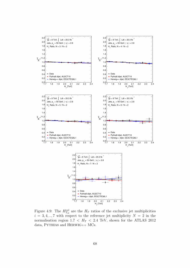
[TeV]T
H1.7 1.8 1.9 2.0 2.1 2.2 2.3 2.4
exl
32
TH
0.0
0.2
0.4
0.6
0.8
1.0
1.2
1.4
1.6
1.8
2.0
2.2 1Ldt = 20.3 fb∫ = 8 TeV, s
| < 2.8η > 50 GeV, | T
Jets, p
Ratio, N = 3 / N = 2T
H
Data
Pythia8 dijet, AU2CT10
Herwig++ dijet, EE3CTEQ6L1
[TeV]T
H1.7 1.8 1.9 2.0 2.1 2.2 2.3 2.4
exl
42
TH
0.0
0.2
0.4
0.6
0.8
1.0
1.2
1.4
1.6
1.8
2.0
2.2 1Ldt = 20.3 fb∫ = 8 TeV, s
| < 2.8η > 50 GeV, | T
Jets, p
Ratio, N = 4 / N = 2T
H
Data
Pythia8 dijet, AU2CT10
Herwig++ dijet, EE3CTEQ6L1
[TeV]T
H1.7 1.8 1.9 2.0 2.1 2.2 2.3 2.4
exl
52
TH
0.0
0.2
0.4
0.6
0.8
1.0
1.2
1.4
1.6
1.8
2.0
2.2 1Ldt = 20.3 fb∫ = 8 TeV, s
| < 2.8η > 50 GeV, | T
Jets, p
Ratio, N = 5 / N = 2T
H
Data
Pythia8 dijet, AU2CT10
Herwig++ dijet, EE3CTEQ6L1
[TeV]T
H1.7 1.8 1.9 2.0 2.1 2.2 2.3 2.4
exl
62
TH
0.0
0.2
0.4
0.6
0.8
1.0
1.2
1.4
1.6
1.8
2.0
2.2 1Ldt = 20.3 fb∫ = 8 TeV, s
| < 2.8η > 50 GeV, | T
Jets, p
Ratio, N = 6 / N = 2T
H
Data
Pythia8 dijet, AU2CT10
Herwig++ dijet, EE3CTEQ6L1
[TeV]T
H1.7 1.8 1.9 2.0 2.1 2.2 2.3 2.4
exl
72
TH
0.0
0.2
0.4
0.6
0.8
1.0
1.2
1.4
1.6
1.8
2.0
2.2 1Ldt = 20.3 fb∫ = 8 TeV, s
| < 2.8η > 50 GeV, | T
Jets, p
Ratio, N = 7 / N = 2T
H
Data
Pythia8 dijet, AU2CT10
Herwig++ dijet, EE3CTEQ6L1
Figure 4.9: The HexlTi2
are the HT ratios of the exclusive jet multiplicitiesi = 3, 4, .., 7 with respect to the reference jet multiplicity N = 2 in thenormalisation region 1.7 < HT < 2.4 TeV, shown for the ATLAS 2012data, PYTHIA8 and HERWIG++ MCs.
68

[TeV]T
H1.7 1.8 1.9 2.0 2.1 2.2 2.3 2.4
inl 32
TH
0.0
0.2
0.4
0.6
0.8
1.0
1.2
1.4
1.6
1.8
2.0
2.2 1Ldt = 20.3 fb∫ = 8 TeV, s
| < 2.8η > 50 GeV, | T
Jets, p
3 / N = 2≥ Ratio, N T
H
Data
Pythia8 dijet, AU2CT10
Herwig++ dijet, EE3CTEQ6L1
[TeV]T
H1.7 1.8 1.9 2.0 2.1 2.2 2.3 2.4
inl 42
TH
0.0
0.2
0.4
0.6
0.8
1.0
1.2
1.4
1.6
1.8
2.0
2.2 1Ldt = 20.3 fb∫ = 8 TeV, s
| < 2.8η > 50 GeV, | T
Jets, p
4 / N = 2≥ Ratio, N T
H
Data
Pythia8 dijet, AU2CT10
Herwig++ dijet, EE3CTEQ6L1
[TeV]T
H1.7 1.8 1.9 2.0 2.1 2.2 2.3 2.4
inl 52
TH
0.0
0.2
0.4
0.6
0.8
1.0
1.2
1.4
1.6
1.8
2.0
2.2 1Ldt = 20.3 fb∫ = 8 TeV, s
| < 2.8η > 50 GeV, | T
Jets, p
5 / N = 2≥ Ratio, N T
H
Data
Pythia8 dijet, AU2CT10
Herwig++ dijet, EE3CTEQ6L1
[TeV]T
H1.7 1.8 1.9 2.0 2.1 2.2 2.3 2.4
inl 62
TH
0.0
0.2
0.4
0.6
0.8
1.0
1.2
1.4
1.6
1.8
2.0
2.2 1Ldt = 20.3 fb∫ = 8 TeV, s
| < 2.8η > 50 GeV, | T
Jets, p
6 / N = 2≥ Ratio, N T
H
Data
Pythia8 dijet, AU2CT10
Herwig++ dijet, EE3CTEQ6L1
[TeV]T
H1.7 1.8 1.9 2.0 2.1 2.2 2.3 2.4
inl 72
TH
0.0
0.2
0.4
0.6
0.8
1.0
1.2
1.4
1.6
1.8
2.0
2.2 1Ldt = 20.3 fb∫ = 8 TeV, s
| < 2.8η > 50 GeV, | T
Jets, p
7 / N = 2≥ Ratio, N T
H
Data
Pythia8 dijet, AU2CT10
Herwig++ dijet, EE3CTEQ6L1
Figure 4.10: The H inlTi2
are the HT ratios of the inclusive jet multiplicitiesi ≥ 3, 4, .., 7 with respect to the reference jet multiplicity N = 2 in thenormalisation region 1.7 < HT < 2.4 TeV, shown for the ATLAS 2012data, PYTHIA8 and HERWIG++ MCs.
69
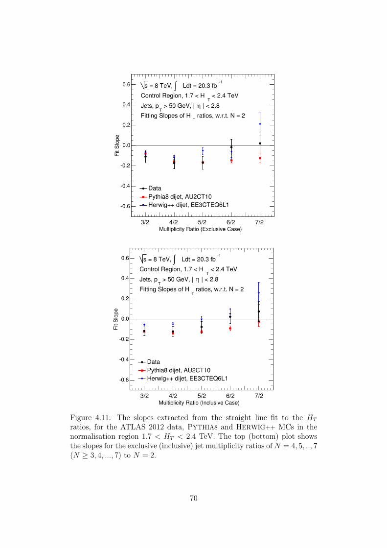
Multiplicity Ratio (Exclusive Case)
Fit S
lop
e
0.6
0.4
0.2
0.0
0.2
0.4
0.6
3/2 4/2 5/2 6/2 7/2
1 Ldt = 20.3 fb∫ = 8 TeV, s
< 2.4 TeVT
Control Region, 1.7 < H
| < 2.8η > 50 GeV, | T
Jets, p
ratios, w.r.t. N = 2T
Fitting Slopes of H
Data
Pythia8 dijet, AU2CT10
Herwig++ dijet, EE3CTEQ6L1
Multiplicity Ratio (Inclusive Case)
Fit S
lop
e
0.6
0.4
0.2
0.0
0.2
0.4
0.6
3/2 4/2 5/2 6/2 7/2
1 Ldt = 20.3 fb∫ = 8 TeV, s
< 2.4 TeVT
Control Region, 1.7 < H
| < 2.8η > 50 GeV, | T
Jets, p
ratios, w.r.t. N = 2T
Fitting Slopes of H
Data
Pythia8 dijet, AU2CT10
Herwig++ dijet, EE3CTEQ6L1
Figure 4.11: The slopes extracted from the straight line fit to the HT
ratios, for the ATLAS 2012 data, PYTHIA8 and HERWIG++ MCs in thenormalisation region 1.7 < HT < 2.4 TeV. The top (bottom) plot showsthe slopes for the exclusive (inclusive) jet multiplicity ratios of N = 4, 5, .., 7(N ≥ 3, 4, ..., 7) to N = 2.
70

Multiplicity Ratio (Exclusive Case)
Fit S
lop
e
0.6
0.4
0.2
0.0
0.2
0.4
0.6
4/3 5/3 6/3 7/3
1Ldt = 20.3 fb∫ = 8 TeV, s
< 2.4 TeVT
Control Region, 1.7 < H
| < 2.8η > 50 GeV, | T
Jets, p
ratios, w.r.t. N = 3T
Fitting Slopes of H
Data
Pythia8 dijet, AU2CT10
Herwig++ dijet, EE3CTEQ6L1
Multiplicity Ratio (Inclusive Case)
Fit S
lop
e
0.6
0.4
0.2
0.0
0.2
0.4
0.6
3/3 4/3 5/3 6/3 7/3
1 Ldt = 20.3 fb∫ = 8 TeV, s
< 2.4 TeVT
Control Region, 1.7 < H
| < 2.8η > 50 GeV, | T
Jets, p
ratios, w.r.t. N = 3T
Fitting Slopes of H
Data
Pythia8 dijet, AU2CT10
Herwig++ dijet, EE3CTEQ6L1
Figure 4.12: The slopes extracted from the straight line fit to the HT
ratios, for the ATLAS 2012 data, PYTHIA8 and HERWIG++ MCs in thenormalisation region 1.7 < HT < 2.4 TeV. The top (bottom) plot showsthe slopes for the exclusive (inclusive) jet multiplicity ratios of N = 4, 5, .., 7(N ≥ 3, 4, ..., 7) to N = 3.
71
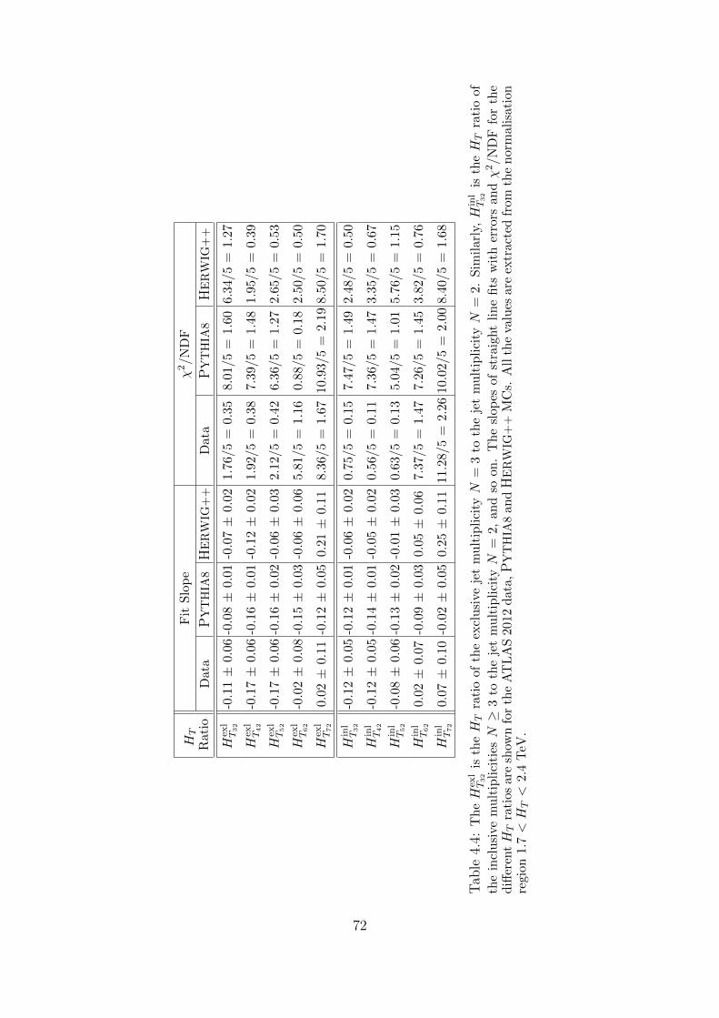
HT
Rat
io
Fit
Slo
pe
χ2/N
DF
Data
PY
TH
IA8
HE
RW
IG+
+D
ata
PY
TH
IA8
HE
RW
IG+
+
Hex
lT32
-0.1
1±
0.06
-0.0
8±
0.01
-0.0
7±
0.02
1.76
/5=
0.35
8.0
1/5
=1.
60
6.34/
5=
1.2
7
Hex
lT42
-0.1
7±
0.06
-0.1
6±
0.01
-0.1
2±
0.02
1.92
/5=
0.38
7.3
9/5
=1.
48
1.95/
5=
0.3
9
Hex
lT52
-0.1
7±
0.06
-0.1
6±
0.02
-0.0
6±
0.03
2.12
/5=
0.42
6.3
6/5
=1.
27
2.65/
5=
0.5
3
Hex
lT62
-0.0
2±
0.08
-0.1
5±
0.03
-0.0
6±
0.06
5.81
/5=
1.16
0.8
8/5
=0.
18
2.50/
5=
0.5
0
Hex
lT72
0.02±
0.11
-0.1
2±
0.05
0.21±
0.11
8.36
/5=
1.67
10.9
3/5
=2.
19
8.50/
5=
1.7
0
Hin
lT32
-0.1
2±
0.05
-0.1
2±
0.01
-0.0
6±
0.02
0.75
/5=
0.15
7.4
7/5
=1.
49
2.48/
5=
0.5
0
Hin
lT42
-0.1
2±
0.05
-0.1
4±
0.01
-0.0
5±
0.02
0.56
/5=
0.11
7.3
6/5
=1.
47
3.35/
5=
0.6
7
Hin
lT52
-0.0
8±
0.06
-0.1
3±
0.02
-0.0
1±
0.03
0.63
/5=
0.13
5.0
4/5
=1.
01
5.76/
5=
1.1
5
Hin
lT62
0.02±
0.07
-0.0
9±
0.03
0.05±
0.06
7.37
/5=
1.47
7.2
6/5
=1.
45
3.82/
5=
0.7
6
Hin
lT72
0.07±
0.10
-0.0
2±
0.05
0.25±
0.11
11.2
8/5
=2.
2610
.02/5
=2.
00
8.40/
5=
1.6
8
Tab
le4.
4:T
heH
exl
T32
isth
eHT
rati
oof
the
excl
usi
veje
tm
ult
ipli
cityN
=3
toth
eje
tm
ult
ipli
cityN
=2.
Sim
ilarl
y,H
inl
T32
isth
eHT
rati
oof
the
incl
usi
vem
ult
ipli
citi
esN≥
3to
the
jet
mu
ltip
lici
tyN
=2,
and
soon
.T
he
slop
esof
stra
ight
lin
efi
tsw
ith
erro
rsan
dχ
2/N
DF
for
the
diff
eren
tHT
rati
osar
esh
own
for
the
AT
LA
S20
12d
ata,
PY
TH
IA8
and
HE
RW
IG+
+M
Cs.
All
the
valu
esar
eex
tract
edfr
om
the
norm
ali
sati
on
regio
n1.
7<HT<
2.4
TeV
.
72

4.5.3 The Signal and the Control Regions1327
In this study, three mutually exclusive regions are defined: the control1328
region, the normalisation region and the signal region with respect to the1329
(N , HT ) variable space. The regions are defined as following:1330
• control region: N = 2 and HT > 1.7 TeV.1331
This region is well-described by SM processes, and no resonances or1332
threshold enhancements have been observed at the LHC.1333
• normalisation region: N ≥ 2 and 1.7 < HT < 2.4 TeV.1334
In this region, the HT distribution for any jet multiplicity N > 2 is1335
normalized to the jet multiplicity N = 2.1336
• signal region: N > 2 and HT > 2.4 TeV.1337
Only this region is searched for possible signals.1338
In summary, the control region does not contain any threshold en-1339
hancement or resonance and the SM processes are dominant in the region.1340
Moreover, microscopic black holes are expected to produce high multiplic-1341
ity final states. Therefore, in the multijet study, the choice of the dijet case1342
is safe for the control region. The flattest region in the HT ratio is chosen1343
as the normalisation region, the sub-region of the control region with best1344
shape invariance. The flatness in the HT ratio ensures the control region1345
fit has a better background estimation for the signal region. To estimate1346
the background for N > 2 a normalisation factor is determined from the1347
normalisation region to normalize the control region fit. Finally, the sig-1348
nal region can be defined beyond the upper threshold of the normalisation1349
region.1350
73

4.5.4 The Background Estimation1351
The QCD background is determined by using an ansatz fitting function,1352
f(x) =p0(1− x)p1
xp2+p3 lnx, (4.4)
where p0, p1, p2 and p3 are the fit parameters and x ≡ HT/√s. The1353
function is fit to the HT distribution for the data instead of x. For a1354
physical background estimation from the HT distributions, the function1355
should be continuously decreasing in an allowed range and have physical1356
values at the tail. This function was already used in invariant mass study1357
for the smooth SM dijet and γ+jet backgrounds in different experiments1358
at both the Tevatron and LHC [80,83,84].1359
The parameter p0 acts as a normalisation factor and does not affect1360
the shape of the fit, but its value depends on the other fit parameters1361
which are highly correlated with the x-dependent factors in equation (4.4).1362
On the other hand, fits with the same shapes and different normalisation1363
factors will have identical p1, p2 and p3 but different p0. Therefore, p0 > 01364
is required to fit any HT distribution for a shape-dependent analysis.1365
The factor (1− x)p1 in the numerator of equation (4.4) controls the1366
upper physical threshold of x. Assuming p1 > 0, the function vanishes1367
as x → 1, since no event can be produced above√s (x > 1). Hence, it1368
is appropriate to require p1 > 0 to maintain the continuously decreasing1369
trend of the QCD background at high x. Furthermore, the function is not1370
required to fit a resonance or increase with HT due to a non-perturbative1371
gravity signal. The function is designed to fit to the background only.1372
For the factor xp2+p3 lnx in the denominator of equation (4.4), p3 is1373
the relevant parameter as x→ 0 because lnx→ −∞ as x→ 0. There are1374
two possibilities1 for the function as x→ 0 depending on the parameter p3.1375
1 The possibility of p3 = 0 is ignored because the function to fit the data has fourparameters, and requiring p3 = 0 changes the function.
74

Fit p0 ±∆p0 p1 ±∆p1 p2 ±∆p2 p3 ±∆p3
parameters 0.03 ± 0.00 4.72 ± 0.18 11.29 ± 0.06 1.57 ± 0.04
Table 4.5: The values of fit parameters (pi) along with errors (∆pi) for the
function f(x) = p0(1−x)p1
xp2+p3 ln x fitted to the dijet HT distribution for the ATLAS2012 data.
The first possibility is that the function approaches infinity as x→ 0, which1376
requires p3 < 0. The value of the function becomes non-physical at x = 0,1377
but it can be avoided by applying a small x cut-off in the experimental HT1378
distributions and the function remains physical in the measured x-range.1379
The second possibility is to have a function maximum in the 0 < x < 11380
range and a decreasing trend as x → 0 by requiring p3 > 0 . The require-1381
ment does not remain physical and intuitive if the function peak lies within1382
the x-range under consideration. This possibility can only be taken into1383
account if the peak of the function lies below the minimum x of the experi-1384
mental HT distributions. In conclusion, all the parameters are constrained1385
to have a monotonically decreasing function trend with a negative slope for1386
the x-range under consideration. The values of all the fit parameters are1387
shown in the Table 4.5. In this study, the resulting experimental limits are1388
for the particular choice of the ansatz function similar to the choice of a1389
benchmark signal model.1390
The function in equation (4.4) is used to fit the control region only.1391
The shape of the control region fit is normalized based on the HT distri-1392
butions in the normalisation region, which is used to determine the back-1393
ground shapes in the signal region. Using the observed number of events1394
compared to the predicted number of SM background events in the signal1395
region, upper limits are set on the production of new physics and micro-1396
scopic black holes.1397
The background prediction along with three sigma uncertainty band1398
75

due to fit parameter errors is shown in Figures 4.13 and 4.14 for both the1399
exclusive and inclusive jet multiplicities. The three sigma uncertainty band1400
is shown because one and two sigma bands are too narrow to be seen clearly.1401
In these figures, there is an overestimation of background for most of jet1402
multiplicity cases in the signal region. In the next subsection, the source1403
of this problem and correction to the background estimation is discussed.1404
4.5.5 Correction to the Background Estimation1405
From Figures 4.7 and 4.8, the QCD MCs show non-invariant effects in the1406
HT distributions. It can be concluded that the non-invariant effects are1407
causing an overestimation of the data-driven background in the signal re-1408
gion. Therefore, correction factors are derived from both the PYTHIA8 and1409
HERWIG++ MCs and applied to the data-driven background to compensate1410
for the HT non-invariance in the signal region. Any possible signal bias can1411
be avoided by using correction factors derived from the QCD MCs. The HT1412
ratio for the MC distributions in the normalisation region can be written1413
as1414 [1
nnom.f
HN>2T
HN=2T
]MC
=[ax
′+ b]
MC, (4.5)
where x′ ≡ HT , nnom.
f is the normalisation factor measured in the nominal1415
normalisation region, i.e. 1.7 < HT < 2.4 TeV, and a and b are the1416
slope and intercept of the straight line, respectively. The straight line fit1417
[ax′
+ b]MC obtained from equation (4.5) is used as a correction factor1418
and applied to the background estimation. For the N > 2 background1419
estimation, by using the shape invariance assumption, the control region1420
fit is multiplied by a normalisation factor (as described in subsection 4.5.4),1421
i.e.1422
fN>2(x) = nnom.f f(x) = nnom.
f
p0(1− x)p1
xp2+p3 lnx, (4.6)
76

[TeV]T
H
2.0 2.5 3.0 3.5 4.0 4.5 5.0
Entr
ies / 0
.1 T
eV
1
10
210
310
410
1
Ldt = 20.3 fb∫ = 8 TeV, s
| < 2.8η > 50 GeV, |T
Jets, p
Multiplicity, N = 2
Data
σ 3±Background
[TeV]T
H
2.0 2.5 3.0 3.5 4.0 4.5 5.0
Entr
ies / 0
.1 T
eV
1
10
210
310
410 1
Ldt = 20.3 fb∫ = 8 TeV, s
| < 2.8η > 50 GeV, |T
Jets, p
Multiplicity, N = 3
Data
σ 3±Background
[TeV]T
H
2.0 2.5 3.0 3.5 4.0 4.5 5.0
Entr
ies / 0
.1 T
eV
1
10
210
310
410 1
Ldt = 20.3 fb∫ = 8 TeV, s
| < 2.8η > 50 GeV, |T
Jets, p
Multiplicity, N = 4
Data
σ 3±Background
[TeV]T
H
2.0 2.5 3.0 3.5 4.0 4.5 5.0
Entr
ies / 0
.1 T
eV
1
10
210
310
410
1
Ldt = 20.3 fb∫ = 8 TeV, s
| < 2.8η > 50 GeV, |T
Jets, p
Multiplicity, N = 5
Data
σ 3±Background
[TeV]T
H
2.0 2.5 3.0 3.5 4.0 4.5 5.0
Entr
ies / 0
.1 T
eV
1
10
210
310
1
Ldt = 20.3 fb∫ = 8 TeV, s
| < 2.8η > 50 GeV, |T
Jets, p
Multiplicity, N = 6
Data
σ 3±Background
[TeV]T
H
2.0 2.5 3.0 3.5 4.0 4.5 5.0
Entr
ies / 0
.1 T
eV
1
10
210
310
1
Ldt = 20.3 fb∫ = 8 TeV, s
| < 2.8η > 50 GeV, |T
Jets, p
Multiplicity, N = 7
Data
σ 3±Background
Figure 4.13: The background estimation for the HT distributions with 3σuncertainty, for the exclusive jet multiplicities N = 2, 3, ..., 7.
77
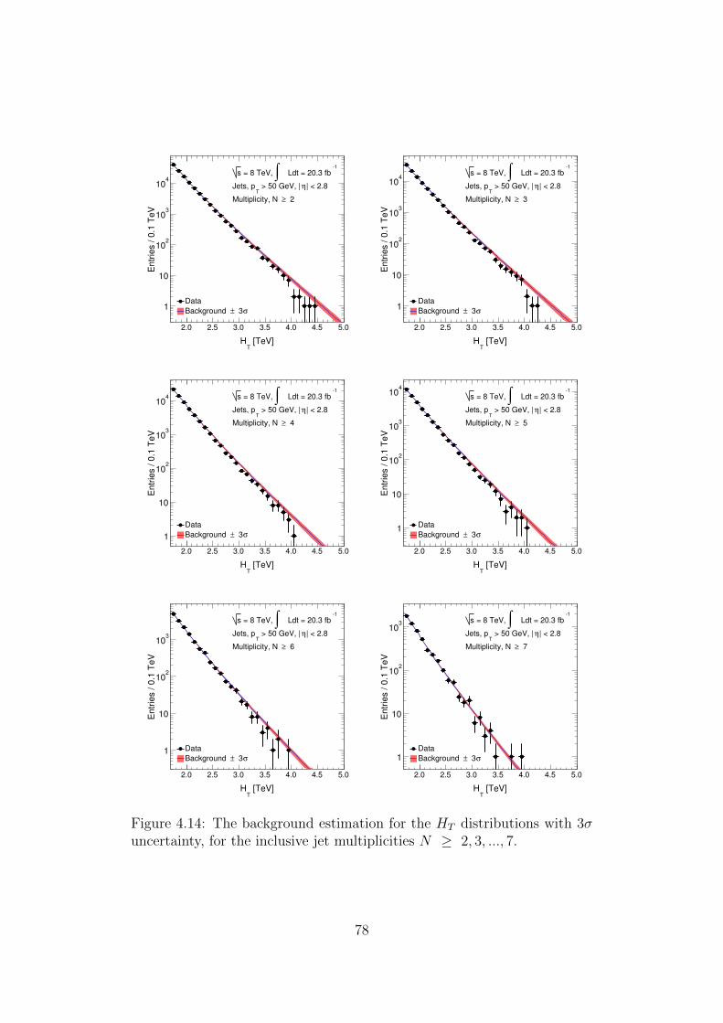
[TeV]T
H
2.0 2.5 3.0 3.5 4.0 4.5 5.0
Entr
ies / 0
.1 T
eV
1
10
210
310
410
1
Ldt = 20.3 fb∫ = 8 TeV, s
| < 2.8η > 50 GeV, |T
Jets, p
2≥Multiplicity, N
Data
σ 3±Background
[TeV]T
H
2.0 2.5 3.0 3.5 4.0 4.5 5.0
Entr
ies / 0
.1 T
eV
1
10
210
310
410
1
Ldt = 20.3 fb∫ = 8 TeV, s
| < 2.8η > 50 GeV, |T
Jets, p
3≥Multiplicity, N
Data
σ 3±Background
[TeV]T
H
2.0 2.5 3.0 3.5 4.0 4.5 5.0
Entr
ies / 0
.1 T
eV
1
10
210
310
410
1
Ldt = 20.3 fb∫ = 8 TeV, s
| < 2.8η > 50 GeV, |T
Jets, p
4≥Multiplicity, N
Data
σ 3±Background
[TeV]T
H
2.0 2.5 3.0 3.5 4.0 4.5 5.0
Entr
ies / 0
.1 T
eV
1
10
210
310
410 1
Ldt = 20.3 fb∫ = 8 TeV, s
| < 2.8η > 50 GeV, |T
Jets, p
5≥Multiplicity, N
Data
σ 3±Background
[TeV]T
H
2.0 2.5 3.0 3.5 4.0 4.5 5.0
Entr
ies / 0
.1 T
eV
1
10
210
310
1
Ldt = 20.3 fb∫ = 8 TeV, s
| < 2.8η > 50 GeV, |T
Jets, p
6≥Multiplicity, N
Data
σ 3±Background
[TeV]T
H
2.0 2.5 3.0 3.5 4.0 4.5 5.0
Entr
ies / 0
.1 T
eV
1
10
210
310
1
Ldt = 20.3 fb∫ = 8 TeV, s
| < 2.8η > 50 GeV, |T
Jets, p
7≥Multiplicity, N
Data
σ 3±Background
Figure 4.14: The background estimation for the HT distributions with 3σuncertainty, for the inclusive jet multiplicities N ≥ 2, 3, ..., 7.
78

where f(x) is the function described in equation (4.4) used to fit the dijet1423
HT distribution and fN>2(x) is the same function multiplied by a normal-1424
isation factor (nnom.f ) used to determine the background for the jet mul-1425
tiplicities N > 2. Now the corrected function fN>2corr. (x) can be written as1426
1427
fN>2corr. (x) = fN>2(x)
[ax
′+ b]
MC=
[nnom.f
p0(1− x)p1
xp2+p3 lnx
] [ax
′+ b]
MC, (4.7)
where x ≡ x′/√s = HT/
√s. Equation (4.7) illustrates that the data-driven1428
background for all the HT distributions other than N = 2 is corrected by1429
the straight line parameters obtained from the HT distributions for the1430
QCD MCs. If the background is corrected by PYTHIA8, then the slope1431
a ≡ aP and intercept b ≡ bP are extracted from the HT distributions for1432
the PYTHIA8 MC. Similarly, a ≡ aH and b ≡ bH are the slope and intercept1433
corresponding to the straight line corrections based on HERWIG++ MC.1434
Finally, both the PYTHIA8 and HERWIG++ MCs are used to ap-1435
ply a final correction on the data-driven background in the signal region.1436
The slope and intercept trends are averaged for both the MC distributions1437
as a ≡ (aP + aH)/2 and b ≡ (bP + bH)/2. The uncorrected background1438
(Buncorr.), PYTHIA8 corrected background (BPcorr.), HERWIG++ corrected1439
background (BHcorr.), and combined PYTHIA8 and HERWIG++ corrected1440
background (BMCcorr.) are shown in Figures 4.15 and 4.16, for the exclusive1441
and inclusive jet multiplicity cases.1442
The uncorrected background (Buncorr.) is corrected by multiplying a1443
correction factor (CF) derived from the MC HT distributions. The cor-1444
rected background can be expressed in terms of correction factors based on1445
PYTHIA8 MC, HERWIG++ MC and both the MCs as1446
BPcorr. = CFPBuncorr., BH
corr. = CFHBuncorr. and BMCcorr. = CFMCBuncorr., (4.8)
where CFP, CFH and CFMC are the correction factors derived from PYTHIA8,1447
79

HERWIG++ and both the MCs, respectively. The uncertainty due to this1448
correction will be discussed in the next section 4.6.1449
4.6 Systematic Uncertainties1450
In this multijet search for microscopic black holes, the main QCD back-1451
ground is directly estimated from the data on the basis of a shape invariance1452
assumption using the ansatz fitting function described in subsection 4.5.4.1453
The ansatz function used in this study is a choice to fit the data. There1454
may be a different arbitrary function that fits the data as well. Therefore,1455
a particular choice of an ansatz function may lead to a systematic uncer-1456
tainty. There are two approaches to handle the systematic uncertainty due1457
to the choice of a specific function. The first approach is to not consider this1458
type of systematic uncertainty and understand the resulting experimental1459
limits based on the particular function. This method is similar to choosing1460
a benchmark signal model for a study, i.e. the ansatz of new physics. The1461
second approach is to use two alternative functions, one that gives larger1462
results while the other gives lower results when compared to the nominal1463
function. This takes the uncertainty due to the choice of function into ac-1464
count. The amount of uncertainty depends again on the choice of the two1465
alternative functions out of many arbitrary choices. In this analysis, the1466
first approach is adopted.1467
The largest uncertainty involved in the background estimation arises1468
due to the MC-based corrections to the non-invariant effects in the HT dis-1469
tributions for different jet multiplicities. The background estimation in1470
the signal region also has uncertainties related to the relative differences1471
from the choice of the normalisation region. Different normalisation ranges1472
will result in different values of normalisation factors and, hence, the back-1473
ground estimation.1474
80

[TeV]T
H
2.5 3.0 3.5 4.0 4.5 5.0
Entr
ies / 0
.1 T
eV
1
10
210
310
1
Ldt = 20.3 fb∫ = 8 TeV, s
| < 2.8η > 50 GeV, |T
Jets, p
> 2.4 TeV T
Signal Region, H
Multiplicity, N = 3
uncorr.B
H
corr.B
P
corr.B
MC
corr.B
Data
[TeV]T
H
2.5 3.0 3.5 4.0 4.5 5.0
Entr
ies / 0
.1 T
eV
1
10
210
310
1
Ldt = 20.3 fb∫ = 8 TeV, s
| < 2.8η > 50 GeV, |T
Jets, p
> 2.4 TeV T
Signal Region, H
Multiplicity, N = 4
uncorr.B
H
corr.B
P
corr.B
MC
corr.B
Data
[TeV]T
H
2.5 3.0 3.5 4.0 4.5 5.0
Entr
ies / 0
.1 T
eV
1
10
210
1
Ldt = 20.3 fb∫ = 8 TeV, s
| < 2.8η > 50 GeV, |T
Jets, p
> 2.4 TeV T
Signal Region, H
Multiplicity, N = 5
uncorr.B
H
corr.B
P
corr.B
MC
corr.B
Data
[TeV]T
H
2.5 3.0 3.5 4.0 4.5 5.0
Entr
ies / 0
.1 T
eV
1
10
210
1
Ldt = 20.3 fb∫ = 8 TeV, s
| < 2.8η > 50 GeV, |T
Jets, p
> 2.4 TeV T
Signal Region, H
Multiplicity, N = 6
uncorr.B
H
corr.B
P
corr.B
MC
corr.B
Data
[TeV]T
H
2.5 3.0 3.5 4.0 4.5 5.0
Entr
ies / 0
.1 T
eV
1
10
210 1
Ldt = 20.3 fb∫ = 8 TeV, s
| < 2.8η > 50 GeV, |T
Jets, p
> 2.4 TeV T
Signal Region, H
Multiplicity, N = 7
uncorr.B
H
corr.B
P
corr.B
MC
corr.B
Data
Figure 4.15: The HT distributions in the signal region, for the exclusivejet multiplicities N = 3, 4, .., 7, and the background estimations from theuncorrected fit (Buncorr.), HERWIG++ MC corrected fit (BH
corr.), PYTHIA8
MC corrected fit (BPcorr.) and the corrected fit based on both the MCs
(BMCcorr.), are shown for the ATLAS 2012 data.
81

[TeV]T
H
2.5 3.0 3.5 4.0 4.5 5.0
Entr
ies / 0
.1 T
eV
1
10
210
310
1
Ldt = 20.3 fb∫ = 8 TeV, s
| < 2.8η > 50 GeV, |T
Jets, p
> 2.4 TeV T
Signal Region, H
3≥Multiplicity, N
uncorr.B
H
corr.B
P
corr.B
MC
corr.B
Data
[TeV]T
H
2.5 3.0 3.5 4.0 4.5 5.0
Entr
ies / 0
.1 T
eV
1
10
210
310
1
Ldt = 20.3 fb∫ = 8 TeV, s
| < 2.8η > 50 GeV, |T
Jets, p
> 2.4 TeV T
Signal Region, H
4≥Multiplicity, N
uncorr.B
H
corr.B
P
corr.B
MC
corr.B
Data
[TeV]T
H
2.5 3.0 3.5 4.0 4.5 5.0
Entr
ies / 0
.1 T
eV
1
10
210
310
1
Ldt = 20.3 fb∫ = 8 TeV, s
| < 2.8η > 50 GeV, |T
Jets, p
> 2.4 TeV T
Signal Region, H
5≥Multiplicity, N
uncorr.B
H
corr.B
P
corr.B
MC
corr.B
Data
[TeV]T
H
2.5 3.0 3.5 4.0 4.5 5.0
Entr
ies / 0
.1 T
eV
1
10
210
1
Ldt = 20.3 fb∫ = 8 TeV, s
| < 2.8η > 50 GeV, |T
Jets, p
> 2.4 TeV T
Signal Region, H
6≥Multiplicity, N
uncorr.B
H
corr.B
P
corr.B
MC
corr.B
Data
[TeV]T
H
2.5 3.0 3.5 4.0 4.5 5.0
Entr
ies / 0
.1 T
eV
1
10
210
1
Ldt = 20.3 fb∫ = 8 TeV, s
| < 2.8η > 50 GeV, |T
Jets, p
> 2.4 TeV T
Signal Region, H
7≥Multiplicity, N
uncorr.B
H
corr.B
P
corr.B
MC
corr.B
Data
Figure 4.16: The HT distributions in the signal region, for the inclusivejet multiplicities N ≥ 3, 4, .., 7, and the background estimations from theuncorrected fit (Buncorr.), HERWIG++ MC corrected fit (BH
corr.), PYTHIA8
MC corrected fit (BPcorr.) and the corrected fit based on both the MCs
(BMCcorr.), are shown for the ATLAS 2012 data.
82

Finally, the typical jet energy uncertainties due to the jet energy1475
resolution (JER) [85] and the jet energy scale (JES) [86] also affect the1476
background estimation. The jet energy uncertainties are comparatively1477
smaller than the uncertainties due to corrections to the non-invariant HT1478
shapes and larger than the uncertainties due to the choice of the normal-1479
isation region. Overall, there are three types of systematic uncertainties1480
involved in this study:1481
• Corrections to non-invariance,1482
• Choice of normalisation region, and1483
• Jet energy uncertainties.1484
By using all these systematic uncertainties, the model-independent and1485
model-dependent limits are calculated, shown in the next section. Micro-1486
scopic black holes are expected to produce a range of jet multiplicities1487
instead of biasing towards any particular multiplicity. It is therefore more1488
intuitive to consider the inclusive jet multiplicities only, i.e. N ≥ 3, 4, ..., 7,1489
for the limit calculations. Also, the large effect of jet migrations from one1490
multiplicity bin to another due to the above-mentioned uncertainties can1491
greatly be suppressed by using the inclusive jet multiplicities. Furthermore,1492
the shape invariance in the normalisation region is better for the inclusive1493
jet multiplicities, which results in reducing all the uncertainties. Therefore,1494
the systematic uncertainties will be described in the following subsections1495
only for the inclusive jet multiplicities.1496
4.6.1 Corrections to Non-Invariance1497
The MC-based corrections applied to the data-driven background, to com-1498
pensate the non-invariant effects, introduce the largest uncertainty in this1499
study. These corrections are derived from the straight line fits to the HT1500
83

ratios in the signal region for the dijet MCs, as described in the subsec-1501
tion 4.5.5. The overall systematic uncertainty due to these corrections to1502
the non-invariance would involve the statistical uncertainty measured from1503
errors on fit parameters and the systematic uncertainty measured from1504
the difference between the fit parameters of the straight lines for the two1505
MCs. The systematic uncertainty due to corrections to the non-invariance1506
(∆Bsyst.corr.) is the ratio of the difference between the straight line fits to the1507
sum of the straight line fits of two MCs over all the HT bins of the signal1508
region, i.e.1509
∆Bsyst.corr. =
∑HT εSR
∣∣(aP + bPx′)− (aH + bHx
′)∣∣
(aP + bPx′) + (aH + bHx
′), (4.9)
where x′ ≡ HT while aP (aH) and bP (bH) are the intercept and slope of the1510
straight line fits corresponding to the PYTHIA8 (HERWIG++) MCs. The1511
statistical uncertainty due to corrections to the non-invariance (∆Bstat.corr.)1512
from these fits is written as1513
∆Bstat.corr. =
1
2
∑HT εSR
√(σP )2 + (σH)2, (4.10)
where σP and σH are the one sigma fit errors corresponding to PYTHIA81514
and HERWIG++, respectively. The total uncertainty on the estimated back-1515
ground due to corrections to the effects from non-invariance (∆Btot.corr.) de-1516
rived from both the MCs in the signal regionsignal region, is written as1517
1518
∆Btot.corr.(%) =
√(∆Bstat.
corr.)2 + (∆Bsyst.
corr.)2 × 100. (4.11)
For different lower thresholds (HminT ) of the signal regions, the number of1519
entries for the data, uncorrected background (Buncorr.), PYTHIA8 correction1520
factor (CFP), HERWIG++ correction factor (CFH), correction factor derived1521
from both the MCs (CFMC), and the uncertainties (∆Bstat.corr., ∆Bsyst.
corr. and1522
∆Btot.corr.) due to CFMC shown in Tables 4.6 to 4.10 for the inclusive jet1523
multiplicities N ≥ 3, 4, ..., 7, respectively.1524
84

HminT Data Buncorr. CFP CFH CFMC ∆Bstat.
corr. (%) ∆Bsyst.corr. (%) ∆Btot.
corr. (%)
2.4 4812 5451.76 0.89 0.94 0.92 9.32 10.15 13.78
2.5 3181 3723.96 0.88 0.93 0.90 8.95 10.50 13.80
2.6 2168 2556.31 0.86 0.92 0.89 8.61 10.86 13.86
2.7 1455 1762.81 0.84 0.92 0.88 8.28 11.23 13.95
2.8 1008 1220.76 0.83 0.91 0.87 7.98 11.60 14.08
2.9 670 848.68 0.81 0.90 0.86 7.70 11.98 14.24
3.0 446 592.11 0.79 0.89 0.84 7.43 12.36 14.42
3.1 321 414.45 0.78 0.89 0.83 7.18 12.75 14.64
3.2 221 290.95 0.76 0.88 0.82 6.95 13.15 14.87
3.3 151 204.79 0.75 0.87 0.81 6.73 13.55 15.13
3.4 96 144.48 0.73 0.86 0.80 6.53 13.96 15.41
3.5 66 102.15 0.71 0.86 0.79 6.33 14.37 15.70
3.6 47 72.34 0.70 0.85 0.77 6.14 14.79 16.02
3.7 32 51.30 0.68 0.84 0.76 5.94 15.22 16.34
3.8 20 36.42 0.67 0.84 0.75 5.75 15.66 16.68
3.9 11 25.88 0.65 0.83 0.74 5.55 16.10 17.03
4.0 4 18.39 0.64 0.82 0.73 5.34 16.56 17.40
4.1 2 13.07 0.62 0.81 0.72 5.12 17.01 17.77
4.2 1 9.28 0.61 0.81 0.71 4.89 17.48 18.15
4.3 0 6.58 0.59 0.80 0.70 4.64 17.96 18.55
4.4 0 4.66 0.58 0.79 0.69 4.37 18.44 18.95
4.5 0 3.28 0.56 0.79 0.67 4.08 18.93 19.37
4.6 0 2.31 0.55 0.78 0.66 3.78 19.44 19.80
4.7 0 1.61 0.53 0.77 0.65 3.45 19.95 20.24
4.8 0 1.11 0.52 0.77 0.64 3.10 20.47 20.70
4.9 0 0.76 0.51 0.76 0.63 2.72 20.99 21.17
5.0 0 0.50 0.50 0.76 0.63 2.33 21.53 21.66
Table 4.6: Number of entries for the data and uncorrected background (Buncorr.), areshown for the jet multiplicity N ≥ 3. The correction factors based on PYTHIA8 MC(CFP), HERWIG++ MC (CFH) and both the MCs (CFMC), are shown corresponding tothe minimum HT thresholds (Hmin
T ). The uncertainties (statistical ∆Bstat.corr., systematic
∆Bstat.corr. and total ∆Btot.
corr.) due to the correction factor CFMC, are also shown for eachHmin
T .
85

HminT Data Buncorr. CFP CFH CFMC ∆Bstat.
corr. (%) ∆Bsyst.corr. (%) ∆Btot.
corr. (%)
2.4 3121 3590.82 0.88 0.94 0.91 11.23 12.85 17.07
2.5 2061 2452.80 0.86 0.93 0.89 10.78 13.32 17.14
2.6 1398 1683.72 0.84 0.92 0.88 10.36 13.80 17.25
2.7 928 1161.08 0.82 0.91 0.87 9.96 14.28 17.42
2.8 648 804.06 0.80 0.90 0.85 9.59 14.78 17.62
2.9 433 558.98 0.78 0.90 0.84 9.25 15.28 17.86
3.0 290 389.99 0.77 0.89 0.83 8.92 15.80 18.14
3.1 206 272.98 0.75 0.88 0.81 8.62 16.32 18.46
3.2 139 191.63 0.73 0.87 0.80 8.34 16.86 18.81
3.3 96 134.89 0.71 0.86 0.79 8.07 17.40 19.18
3.4 62 95.17 0.69 0.85 0.77 7.81 17.96 19.58
3.5 40 67.28 0.67 0.85 0.76 7.57 18.52 20.01
3.6 25 47.65 0.65 0.84 0.75 7.33 19.10 20.46
3.7 17 33.79 0.64 0.83 0.73 7.09 19.69 20.93
3.8 9 23.99 0.62 0.82 0.72 6.85 20.30 21.42
3.9 4 17.04 0.60 0.81 0.71 6.61 20.91 21.93
4.0 1 12.11 0.58 0.81 0.69 6.36 21.54 22.46
4.1 0 8.61 0.56 0.80 0.68 6.09 22.18 23.00
4.2 0 6.11 0.54 0.79 0.67 5.81 22.84 23.56
4.3 0 4.33 0.53 0.78 0.65 5.51 23.50 24.14
4.4 0 3.07 0.51 0.77 0.64 5.19 24.19 24.74
4.5 0 2.16 0.49 0.77 0.63 4.85 24.89 25.36
4.6 0 1.52 0.48 0.76 0.62 4.48 25.60 25.99
4.7 0 1.06 0.46 0.75 0.61 4.09 26.34 26.65
4.8 0 0.73 0.44 0.74 0.59 3.67 27.08 27.33
4.9 0 0.50 0.43 0.74 0.58 3.23 27.85 28.04
5.0 0 0.33 0.42 0.73 0.57 2.76 28.63 28.77
Table 4.7: Number of entries for the data and uncorrected background (Buncorr.), areshown for the jet multiplicity N ≥ 4. The correction factors based on PYTHIA8 MC(CFP), HERWIG++ MC (CFH) and both the MCs (CFMC), are shown corresponding tothe minimum HT thresholds (Hmin
T ). The uncertainties (statistical ∆Bstat.corr., systematic
∆Bstat.corr. and total ∆Btot.
corr.) due to the correction factor CFMC, are also shown for eachHmin
T .
86

HminT Data Buncorr. CFP CFH CFMC ∆Bstat.
corr. (%) ∆Bsyst.corr. (%) ∆Btot.
corr. (%)
2.4 1675 1915.29 0.88 0.96 0.92 14.44 16.25 21.74
2.5 1134 1308.28 0.86 0.95 0.90 13.86 16.85 21.82
2.6 770 898.07 0.84 0.94 0.89 13.31 17.46 21.96
2.7 500 619.30 0.81 0.93 0.87 12.80 18.09 22.16
2.8 345 428.87 0.79 0.92 0.86 12.31 18.73 22.41
2.9 230 298.15 0.77 0.91 0.84 11.86 19.38 22.72
3.0 156 208.02 0.75 0.90 0.83 11.43 20.04 23.07
3.1 106 145.60 0.73 0.89 0.81 11.03 20.73 23.48
3.2 75 102.21 0.71 0.89 0.80 10.65 21.42 23.93
3.3 50 71.95 0.68 0.88 0.78 10.30 22.13 24.41
3.4 31 50.76 0.66 0.87 0.77 9.96 22.86 24.94
3.5 19 35.89 0.64 0.86 0.75 9.63 23.61 25.50
3.6 12 25.41 0.62 0.85 0.74 9.32 24.37 26.09
3.7 9 18.02 0.60 0.84 0.72 9.01 25.15 26.72
3.8 5 12.80 0.58 0.83 0.71 8.70 25.96 27.37
3.9 3 9.09 0.56 0.82 0.69 8.38 26.78 28.06
4.0 1 6.46 0.54 0.82 0.68 8.05 27.62 28.77
4.1 0 4.59 0.52 0.81 0.66 7.71 28.48 29.50
4.2 0 3.26 0.50 0.80 0.65 7.34 29.36 30.27
4.3 0 2.31 0.48 0.79 0.63 6.96 30.27 31.06
4.4 0 1.64 0.46 0.78 0.62 6.55 31.20 31.88
4.5 0 1.15 0.44 0.77 0.61 6.12 32.15 32.73
4.6 0 0.81 0.42 0.77 0.59 5.65 33.13 33.61
4.7 0 0.56 0.40 0.76 0.58 5.16 34.14 34.52
4.8 0 0.39 0.38 0.75 0.57 4.63 35.17 35.47
4.9 0 0.27 0.36 0.74 0.55 4.07 36.23 36.46
5.0 0 0.18 0.35 0.74 0.54 3.48 37.32 37.49
Table 4.8: Number of entries for the data and uncorrected background (Buncorr.), areshown for the jet multiplicity N ≥ 5. The correction factors based on PYTHIA8 MC(CFP), HERWIG++ MC (CFH) and both the MCs (CFMC), are shown corresponding tothe minimum HT thresholds (Hmin
T ). The uncertainties (statistical ∆Bstat.corr., systematic
∆Bstat.corr. and total ∆Btot.
corr.) due to the correction factor CFMC, are also shown for eachHmin
T .
87

HminT Data Buncorr. CFP CFH CFMC ∆Bstat.
corr. (%) ∆Bsyst.corr. (%) ∆Btot.
corr. (%)
2.4 764 845.88 0.89 0.99 0.94 21.67 19.62 29.23
2.5 522 577.80 0.87 0.98 0.93 20.77 20.35 29.08
2.6 354 396.63 0.84 0.97 0.91 19.93 21.09 29.02
2.7 233 273.51 0.82 0.96 0.89 19.14 21.85 29.05
2.8 160 189.41 0.79 0.96 0.87 18.39 22.63 29.16
2.9 107 131.68 0.77 0.95 0.86 17.68 23.43 29.35
3.0 65 91.87 0.74 0.94 0.84 17.02 24.25 29.62
3.1 44 64.30 0.72 0.93 0.82 16.40 25.08 29.97
3.2 27 45.14 0.70 0.92 0.81 15.82 25.94 30.38
3.3 19 31.77 0.67 0.91 0.79 15.27 26.82 30.86
3.4 11 22.42 0.65 0.90 0.77 14.74 27.73 31.40
3.5 8 15.85 0.62 0.89 0.76 14.24 28.65 32.00
3.6 4 11.22 0.60 0.88 0.74 13.76 29.61 32.65
3.7 3 7.96 0.58 0.87 0.72 13.28 30.58 33.34
3.8 1 5.65 0.55 0.86 0.71 12.81 31.59 34.08
3.9 1 4.02 0.53 0.85 0.69 12.33 32.62 34.87
4.0 0 2.85 0.51 0.84 0.67 11.83 33.68 35.70
4.1 0 2.03 0.48 0.83 0.66 11.32 34.77 36.57
4.2 0 1.44 0.46 0.82 0.64 10.79 35.89 37.48
4.3 0 1.02 0.44 0.81 0.62 10.22 37.05 38.43
4.4 0 0.72 0.41 0.80 0.61 9.62 38.24 39.43
4.5 0 0.51 0.39 0.80 0.59 8.98 39.46 40.47
4.6 0 0.36 0.37 0.79 0.58 8.30 40.73 41.56
4.7 0 0.25 0.35 0.78 0.56 7.57 42.03 42.71
4.8 0 0.17 0.33 0.77 0.55 6.80 43.37 43.90
4.9 0 0.12 0.31 0.76 0.54 5.98 44.76 45.16
5.0 0 0.08 0.29 0.76 0.52 5.11 46.19 46.47
Table 4.9: Number of entries for the data and uncorrected background (Buncorr.), areshown for the jet multiplicity N ≥ 6. The correction factors based on PYTHIA8 MC(CFP), HERWIG++ MC (CFH) and both the MCs (CFMC), are shown corresponding tothe minimum HT thresholds (Hmin
T ). The uncertainties (statistical ∆Bstat.corr., systematic
∆Bstat.corr. and total ∆Btot.
corr.) due to the correction factor CFMC, are also shown for eachHmin
T .
88

HminT Data Buncorr. CFP CFH CFMC ∆Bstat.
corr. (%) ∆Bsyst.corr. (%) ∆Btot.
corr. (%)
2.4 296 308.81 0.92 1.07 0.99 36.96 23.02 43.54
2.5 196 210.94 0.89 1.06 0.98 35.37 23.82 42.64
2.6 138 144.80 0.86 1.05 0.96 33.87 24.64 41.88
2.7 86 99.85 0.84 1.04 0.94 32.45 25.48 41.26
2.8 62 69.15 0.81 1.03 0.92 31.11 26.35 40.77
2.9 44 48.07 0.78 1.01 0.90 29.85 27.23 40.41
3.0 24 33.54 0.76 1.00 0.88 28.67 28.14 40.18
3.1 18 23.48 0.73 0.99 0.86 27.56 29.08 40.06
3.2 10 16.48 0.70 0.98 0.84 26.51 30.04 40.06
3.3 7 11.60 0.68 0.97 0.82 25.52 31.02 40.17
3.4 3 8.18 0.65 0.96 0.80 24.59 32.04 40.39
3.5 2 5.79 0.62 0.95 0.79 23.70 33.08 40.69
3.6 2 4.10 0.60 0.94 0.77 22.84 34.15 41.09
3.7 2 2.91 0.57 0.93 0.75 22.01 35.26 41.56
3.8 1 2.06 0.55 0.92 0.73 21.19 36.39 42.11
3.9 1 1.47 0.52 0.90 0.71 20.37 37.57 42.73
4.0 0 1.04 0.49 0.89 0.69 19.53 38.77 43.42
4.1 0 0.74 0.47 0.88 0.68 18.67 40.02 44.16
4.2 0 0.53 0.44 0.87 0.66 17.78 41.30 44.97
4.3 0 0.37 0.42 0.86 0.64 16.84 42.63 45.83
4.4 0 0.26 0.39 0.85 0.62 15.85 43.99 46.76
4.5 0 0.19 0.37 0.84 0.61 14.79 45.41 47.76
4.6 0 0.13 0.35 0.83 0.59 13.67 46.87 48.82
4.7 0 0.09 0.32 0.82 0.57 12.48 48.38 49.96
4.8 0 0.06 0.30 0.81 0.56 11.21 49.94 51.19
4.9 0 0.04 0.28 0.81 0.54 9.86 51.56 52.50
5.0 0 0.03 0.26 0.80 0.53 8.44 53.24 53.90
Table 4.10: Number of entries for the data and uncorrected background (Buncorr.), areshown for the jet multiplicity N ≥ 7. The correction factors based on PYTHIA8 MC(CFP), HERWIG++ MC (CFH) and both the MCs (CFMC), are shown corresponding tothe minimum HT thresholds (Hmin
T ). The uncertainties (statistical ∆Bstat.corr., systematic
∆Bstat.corr. and total ∆Btot.
corr.) due to the correction factor CFMC, are also shown for eachHmin
T .
89

4.6.2 Choice of Normalisation Region1525
The ansatz function f(x) is only used for the baseline case of multiplicity1526
two. For all other multiplicities, N > 2, the same function is normalized1527
to determine the number of background events in the signal region, i.e.1528
fN>2(x) = nnom.f f(x) (shown in equation 4.6). The nominal normalisation1529
factor nnom.f measured in the normalisation region is used to normalize the1530
f(x) to the fN>2(x). The sensitivity of the normalisation factor has been1531
studied by sliding the upper and lower boundaries of the nominal normal-1532
isation region by 0.1 TeV on either side. The normalisation factor nf is1533
measured in different normalisation ranges and compared with the nnom.f .1534
The normalisation factor nf corresponding to any normalisation region is1535
defined as1536
nf =nnum.f
nden.f
, (4.12)
where nnum.f and nden.
f are the numerator and denominator of nf correspond-1537
ing to any normalisation region (NR) and defined as1538
nnum.f =
N>2∑HT εNR
HT and nden.f =
N=2∑HT εNR
HT . (4.13)
The statistical uncertainty (∆nstat.f ) for the normalisation factor nf can be1539
written as1540
∆nstat.f = nf
√1
nnum.f
+1
nden.f
, (4.14)
whereas the systematic uncertainty (∆nsyst.f ) corresponding to nf is written1541
as1542
∆nsyst.f =
∣∣nnom.f − nf
∣∣ . (4.15)
The total uncertainty due to the choice of the normalisation region can be1543
written as1544
∆nf (%) =1
nnom.f
[√(∆nstat.
f )2 + (∆nsyst.f )2
]× 100. (4.16)
90

In Table 4.11, the statistical uncertainty ∆nstat.f , systematic uncertainty1545
∆nsyst.f and the total uncertainty (∆nf ) due to the choice of the normalisa-1546
tion region are shown for inclusive jet multiplicities. In order to compensate1547
the uncertainties from all the possible choices of the normalisation region,1548
the maximum ∆nf is chosen for the limit calculations. Typically this un-1549
certainty remains less than 3%.1550
4.6.3 Jet Energy Uncertainties1551
The jet energy measured in the ATLAS calorimeters is corrected because of1552
the non-compensating response of the calorimeters [87] and energy losses in1553
the bad calorimeter regions (as discussed in Appendix A). The correction1554
is called as jet energy scale (JES) [86]. Due to limited resolution of the1555
detector, the effect of jet energy resolution (JER) is also measured by using1556
some dedicated analyses, as discussed in Ref. [85]. The uncertainties on1557
the JES and JER are also calculated in Ref. [85, 86]. In this analysis,1558
the uncertainties due to the JES and JER uncertainties are measured and1559
collectively referred to as the jet energy uncertainties. The JER uncertainty1560
depends on pseudorapidity, transverse momentum, transverse energy and1561
azimuthal angle. The JES uncertainty also depends on the same variables1562
but, in addition, it uses the number of primary vertices (NPV) and average1563
number of interactions per bunch crossing (µ) variables in order to take the1564
pileup uncertainty effects into account. The effects of both uncertainties1565
on the HT distributions are computed using data, for each jet multiplicity1566
and as a function of HminT .1567
In order to estimate the effect of the JES uncertainty, the pT of1568
all the jets are modified by the JES uncertainty and the HT distribution1569
is recomputed. Since the exclusion limits in this study are calculated on1570
the basis of counting experiments2, the effects of JES uncertainty in the1571
2 The number of data events are counted for each HminT .
91
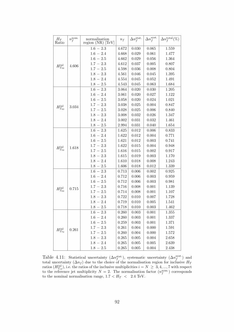
HTRatio
nnom.f normalisation
region (NR) [TeV]nf ∆nstat.f ∆nsyst.f ∆ntotalf (%)
H inlT32
4.606
1.6 − 2.3 4.672 0.030 0.065 1.559
1.6 − 2.4 4.668 0.029 0.061 1.477
1.6 − 2.5 4.662 0.029 0.056 1.364
1.7 − 2.3 4.612 0.037 0.005 0.807
1.7 − 2.5 4.598 0.036 0.008 0.804
1.8 − 2.3 4.561 0.046 0.045 1.395
1.8 − 2.4 4.554 0.045 0.052 1.491
1.8 − 2.5 4.543 0.045 0.063 1.684
H inlT42
3.034
1.6 − 2.3 3.064 0.020 0.030 1.205
1.6 − 2.4 3.061 0.020 0.027 1.122
1.6 − 2.5 3.058 0.020 0.024 1.021
1.7 − 2.3 3.038 0.025 0.004 0.847
1.7 − 2.5 3.028 0.025 0.006 0.840
1.8 − 2.3 3.008 0.032 0.026 1.347
1.8 − 2.4 3.002 0.031 0.032 1.461
1.8 − 2.5 2.994 0.031 0.040 1.654
H inlT52
1.618
1.6 − 2.3 1.625 0.012 0.006 0.833
1.6 − 2.4 1.622 0.012 0.004 0.771
1.6 − 2.5 1.621 0.012 0.003 0.741
1.7 − 2.3 1.622 0.015 0.004 0.948
1.7 − 2.5 1.616 0.015 0.002 0.917
1.8 − 2.3 1.615 0.019 0.003 1.170
1.8 − 2.4 1.610 0.018 0.008 1.243
1.8 − 2.5 1.606 0.018 0.012 1.339
H inlT62
0.715
1.6 − 2.3 0.713 0.006 0.002 0.925
1.6 − 2.4 0.712 0.006 0.003 0.959
1.6 − 2.5 0.712 0.006 0.003 0.981
1.7 − 2.3 0.716 0.008 0.001 1.139
1.7 − 2.5 0.714 0.008 0.001 1.107
1.8 − 2.3 0.722 0.010 0.007 1.728
1.8 − 2.4 0.719 0.010 0.005 1.541
1.8 − 2.5 0.718 0.010 0.003 1.462
H inlT72
0.261
1.6 − 2.3 0.260 0.003 0.001 1.355
1.6 − 2.4 0.260 0.003 0.001 1.337
1.6 − 2.5 0.259 0.003 0.001 1.371
1.7 − 2.3 0.261 0.004 0.000 1.591
1.7 − 2.5 0.260 0.004 0.000 1.572
1.8 − 2.3 0.265 0.005 0.004 2.658
1.8 − 2.4 0.265 0.005 0.005 2.639
1.8 − 2.5 0.265 0.005 0.004 2.438
Table 4.11: Statistical uncertainty (∆nstat.f ), systematic uncertainty (∆nsyst.f ) andtotal uncertainty (∆nf ) due to the choice of the normalisation region for inclusive HT
ratios (H inlTi2
), i.e. the ratios of the inclusive multiplicities i = N ≥ 3, 4, ..., 7 with respectto the reference jet multiplicity N = 2. The normalisation factor (nnom.
f ) correspondsto the nominal normalisation range, 1.7 < HT < 2.4 TeV.
92

jet pT are assumed to be propagated in the modified HT . For each bin of1572
HminT , the difference between the modified HT distribution (HJES
T ) and the1573
nominal HT distribution (HnomT ) is used to define the systematic uncertainty1574
(∆JES), i.e.,1575
∆JES =HJEST −Hnom
T
HnomT
. (4.17)
To quantify the effects of the JER uncertainty on the HT distribu-1576
tion, the jet pT resolution is smeared according to the JER uncertainty1577
by generating five hundred pseudo datasets. The difference between the1578
HT distributions constructed from the datasets ( HJER1T , HJER2
T , ..., HJER500T )1579
and the HnomT , on bin-by-bin basis, is used to define quantities ∆JER1,1580
∆JER2,...,∆JER500, i.e.,1581
∆JERi =HJERiT −Hnom
T
HnomT
, (4.18)
where i = 1, 2, ..., 500 is an integer index corresponding to the dataset1582
number. The final systematic uncertainty due to effects of JER uncertainty1583
is defined from the mean and root mean square values of the gaussian1584
distribution of ∆JERi. The ∆JERi gaussian distributions in different HminT1585
bins, for the jet multiplicity N ≥ 3, are shown as representative cases in1586
Figure 4.17.1587
Typically, the effect of JER uncertainty is 1 − 3%, whereas the ef-1588
fect of JES uncertainty remains 3 − 5%, depending on the HminT for the1589
signal region and the jet multiplicity. The overall jet energy uncertainty is1590
obtained by adding JER and JES uncertainties in quadrature. The effect1591
of jet energy uncertainties on the background estimation remains smaller1592
as compared to the uncertainty due to corrections to non-invariance in HT1593
with jet multiplicity.1594
93

iJER∆
0.02 0.01 0.00 0.01 0.02 0.03 0.04 0.05 0.06
Nu
mb
er
of
Pse
ud
o D
ata
se
ts
0
10
20
30
40
50
60
70
80
90
1
Ldt = 20.3 fb∫ = 8 TeV, s
| < 2.8η > 50 GeV, |T
Jets, p
= 2.7 TeVmin
T for Hi
JER∆
3≥Multiplicity, N
iJER∆
0.04 0.02 0.00 0.02 0.04 0.06 0.08 0.10
Nu
mb
er
of
Pse
ud
o D
ata
se
ts
0
10
20
30
40
50
60
70
80
1
Ldt = 20.3 fb∫ = 8 TeV, s
| < 2.8η > 50 GeV, |T
Jets, p
= 3 TeVmin
T for Hi
JER∆
3≥Multiplicity, N
iJER∆
0.10 0.08 0.06 0.04 0.02 0.00 0.02 0.04 0.06 0.08 0.10
Nu
mb
er
of
Pse
ud
o D
ata
se
ts
0
10
20
30
40
50
60
70
80
90
100
1
Ldt = 20.3 fb∫ = 8 TeV, s
| < 2.8η > 50 GeV, |T
Jets, p
= 3.3 TeVmin
T for Hi
JER∆
3≥Multiplicity, N
iJER∆
0.10 0.05 0.00 0.05 0.10
Nu
mb
er
of
Pse
ud
o D
ata
se
ts
0
20
40
60
80
100
120
140
160
180
1
Ldt = 20.3 fb∫ = 8 TeV, s
| < 2.8η > 50 GeV, |T
Jets, p
= 3.6 TeVmin
T for Hi
JER∆
3≥Multiplicity, N
iJER∆
0.5 0.4 0.3 0.2 0.1 0.0 0.1 0.2 0.3 0.4 0.5
Nu
mb
er
of
Pse
ud
o D
ata
se
ts
0
20
40
60
80
100
120
140
160
180
200
2201
Ldt = 20.3 fb∫ = 8 TeV, s
| < 2.8η > 50 GeV, |T
Jets, p
= 3.9 TeVmin
T for Hi
JER∆
3≥Multiplicity, N
iJER∆
0.8 0.6 0.4 0.2 0.0 0.2 0.4 0.6 0.8 1.0
Nu
mb
er
of
Pse
ud
o D
ata
se
ts
0
50
100
150
200
250
300
1
Ldt = 20.3 fb∫ = 8 TeV, s
| < 2.8η > 50 GeV, |T
Jets, p
= 4 TeVmin
T for Hi
JER∆
3≥Multiplicity, N
Figure 4.17: The ∆JERi = HJERiT −Hnom
T
HnomT
gaussian distributions of five
hundred pseudo datasets, i.e., i = 1, 2, .., 500, corresponding to HminT =
2.7, 3.0, 3.3, 3.6, 3.9, 4.0 TeV, for the jet multiplicities N ≥ 3, are shown for theATLAS 2012 data. For a given pseudo dataset i, the HT distribution with theeffect of jet energy resolution (JER) uncertainty is defined as HJERi
T , whereasthe nominal HT distribution is defined as Hnom
T .
94

4.6.4 Summary of Systematics1595
In this subsection, all the systematic uncertainties described in the previ-1596
ous three subsections are summarized. For the inclusive jet multiplicities1597
N ≥ 3, 4, ..., 7, the data and estimated background along with the total1598
uncertainty are shown in Figure 4.18, as a function of HminT . For each mul-1599
tiplicity, the uncertainty band due to all the systematics, at the each HminT ,1600
is obtained by adding all the uncertainties in quadrature. The different un-1601
certainties may increase or decrease the estimated background, producing1602
an asymmetric uncertainty band, as shown in Figure 4.18.1603
From Figure 4.18, the total uncertainty to the background estima-1604
tion increases with the decreasing statistics with decreasing HminT and from1605
one inclusive multiplicity case to the higher one. Therefore, the lowest1606
statistics case, i.e. N ≥ 7 (the highest inclusive multiplicity in this study),1607
has larger uncertainties than the other multiplicities corresponding to the1608
same HminT values. The shape invariance is also affected by statistics, there-1609
fore, the contribution of uncertainty due to non-invariance is dominant in1610
the low statistics region. As a result, the larger overestimation of the back-1611
ground is observed in the high HminT region. Similarly, for a given Hmin
T , the1612
overestimation of the background increases from a lower multiplicity to the1613
higher one. The uncertainty due to the choice of the normalisation region1614
has a constant effect along the whole range of the HminT (as discussed in1615
subsection 4.6.2), for any inclusive multiplicity. Finally, the jet energy un-1616
certainties contribute significantly in the overall band of total uncertainty,1617
and also increase with the increase in HminT .1618
For N ≥ 3, N ≥ 4 and N ≥ 5, the amount of total uncertainty1619
typically remains in the 15-35% and 35-70% ranges, in the 2.4 < HminT ≤1620
3.5 TeV and 3.6 < HminT ≤ 4.5 TeV regions, respectively. For higher inclu-1621
sive cases, i.e. N ≥ 6 and N ≥ 7, the amount of total uncertainties typically1622
95

lies in the 30-50% and 50-70% ranges, in the 2.4 < HminT ≤ 3.5 TeV and1623
3.6 < HminT ≤ 4.5 TeV regions, respectively. For the Hmin
T > 4.5 TeV region,1624
all the multiplicities have a total uncertainty in the 75-100% range.1625
The plots in Figure 4.18 as a function of HminT indicate an accumu-1626
lative representation of the data and estimated background from the plots1627
shown in Figure 4.16. The data points, from Figure 4.16, fluctuate above1628
and below the estimated background whereas they are always below the1629
estimated background in Figure 4.18. Therefore, another way to visualize1630
the data and estimated background, as a function of HminT , is shown in Fig-1631
ure 4.19. In this figure, the accumulated background shown for different1632
inclusive multiplicities is estimated by excluding the background from the1633
empty data-bins. In this representation, the data and background agree-1634
ment is improved as compared to shown in Figure 4.18.1635
There is no excess of data events found above the estimated back-1636
ground, therefore, model-inpedent and mode-dependent exclusion limits are1637
set at the 95% confidence level (CL). The data and background shown in1638
Figure 4.18 are within one sigma uncertainty. The one sigma agreement can1639
also be seen later from the model-independent exclusion limits. Moreover,1640
the exclusion limits are set in the high HT region, i.e., including the region1641
with empty data bins, therefore, the results obtained from Figure 4.18 are1642
used for calculating limits.1643
4.7 Exclusion Limits1644
The exclusion limits are calculated as a function of HminT for the inclusive jet1645
multiplicities. In the signal region, different HT > HminT values are chosen1646
and counting experiments are performed as a function of HminT . The upper1647
limits are calculated by using a frequentist CLs method [88,89]. Exclusion1648
limits on the production of new physics and black holes are set by taking1649
96

[TeV]min
TH
2.5 3.0 3.5 4.0 4.5
Entr
ies / 0
.1 T
eV
1
10
210
310
410
1
Ldt = 20.3 fb∫ = 8 TeV, s
| < 2.8η > 50 GeV, |T
Jets, p
3≥Multiplicity, N
Data
Background
[TeV]min
TH
2.5 3.0 3.5 4.0 4.5
Entr
ies / 0
.1 T
eV
1
10
210
310
410
1
Ldt = 20.3 fb∫ = 8 TeV, s
| < 2.8η > 50 GeV, |T
Jets, p
4≥Multiplicity, N
Data
Background
[TeV]min
TH
2.5 3.0 3.5 4.0 4.5
Entr
ies / 0
.1 T
eV
1
10
210
310
410
1
Ldt = 20.3 fb∫ = 8 TeV, s
| < 2.8η > 50 GeV, |T
Jets, p
5≥Multiplicity, N
Data
Background
[TeV]min
TH
2.5 3.0 3.5 4.0 4.5
Entr
ies / 0
.1 T
eV
1
10
210
310
410
1
Ldt = 20.3 fb∫ = 8 TeV, s
| < 2.8η > 50 GeV, |T
Jets, p
6≥Multiplicity, N
Data
Background
[TeV]min
TH
2.5 3.0 3.5 4.0 4.5
Entr
ies / 0
.1 T
eV
1
10
210
310
410
1
Ldt = 20.3 fb∫ = 8 TeV, s
| < 2.8η > 50 GeV, |T
Jets, p
7≥Multiplicity, N
Data
Background
Figure 4.18: The HminT distributions, for the inclusive jet multiplicities
N ≥ 3, 4, ..., 7, are shown for the ATLAS 2012 data and predicted backgroundalong with total uncertainty.
97

[TeV]min
TH
2.5 3.0 3.5 4.0 4.5
Entr
ies / 0
.1 T
eV
1
10
210
310
410
1
Ldt = 20.3 fb∫ = 8 TeV, s
| < 2.8η > 50 GeV, |T
Jets, p
3≥Multiplicity, N
Data
Background
[TeV]min
TH
2.5 3.0 3.5 4.0 4.5
Entr
ies / 0
.1 T
eV
1
10
210
310
410
1
Ldt = 20.3 fb∫ = 8 TeV, s
| < 2.8η > 50 GeV, |T
Jets, p
4≥Multiplicity, N
Data
Background
[TeV]min
TH
2.5 3.0 3.5 4.0 4.5
Entr
ies / 0
.1 T
eV
1
10
210
310
410
1
Ldt = 20.3 fb∫ = 8 TeV, s
| < 2.8η > 50 GeV, |T
Jets, p
5≥Multiplicity, N
Data
Background
[TeV]min
TH
2.5 3.0 3.5 4.0 4.5
Entr
ies / 0
.1 T
eV
1
10
210
310
410
1
Ldt = 20.3 fb∫ = 8 TeV, s
| < 2.8η > 50 GeV, |T
Jets, p
6≥Multiplicity, N
Data
Background
[TeV]min
TH
2.5 3.0 3.5 4.0 4.5
Entr
ies / 0
.1 T
eV
1
10
210
310
410
1
Ldt = 20.3 fb∫ = 8 TeV, s
| < 2.8η > 50 GeV, |T
Jets, p
7≥Multiplicity, N
Data
Background
Figure 4.19: The HminT distributions, for the inclusive jet multiplicities
N ≥ 3, 4, ..., 7, are shown for the ATLAS 2012 data and predicted backgroundalong with total uncertainty. The background is estimated by dropping theempty data bins in the HT distributions.
98

all the three types of systematic uncertainties described in section 4.6 into1650
account. The 2.8% luminosity uncertainty is also used in the upper limit1651
calculations. The model-independent upper limits are shown in the next1652
subsection.1653
4.7.1 Model-Independent Limits1654
Model-independent upper limits are calculated at the 95% CL on cross1655
section times the acceptance for new physics production in the high HT1656
inclusive multijet final states for N ≥ 2, 3, ..., 7, as shown in Figure 4.20.1657
These figures show the observed and expected limits along with the one and1658
two standard deviation bands for the expected limits. The observed limits1659
are obtained from the data, whereas the expected limit is the median of1660
the distribution of the limits at the 95% CL generated by pseudo datasets.1661
The pseudo datasets assume a background-only model and are generated1662
by randomly fluctuating the predicted background value. A total of 25001663
pseudo datasets are used in this study and an upper limit is calculated for1664
each one of them. Finally, the expected limit is computed by determining1665
the median of the distribution of the upper limits obtained from all the1666
pseudo datasets. The one and two sigma bands are the 68% and 95%1667
confidence intervals around the median value.1668
The observed limits typically lie below the expected limits within1669
one sigma uncertainty. The exclusion limit on the cross section times ac-1670
ceptance times efficiency3 is 0.29 fb to 0.14 fb for N ≥ 3 to N ≥ 7 for1671
the high-HT , i.e. HT > 4.0 TeV. The limits as a function of the HminT and1672
jet multiplicity are shown in Table 4.12. In order to observe variation of1673
exclusion limits with HT and multijet final states, upper limits on cross1674
section times acceptance times efficiency at the 95% CL as a function of1675
the inclusive jet multiplicities for fixed HminT values, are also shown in Fig-1676
3 These are the acceptance and efficiency of the detector.
99

ure 4.21. For HminT = 2.5, 3.0 and 3.5 TeV, limits decrease with the increase1677
in jet multiplicity. The HminT = 4.0 TeV case looks almost flat for N ≥ 41678
and beyond, whereas the HminT = 4.5 and 5 TeV cases are flat for all the in-1679
clusive multijet final states because no data events are in the HT > 4.5 TeV1680
region. Moreover, exclusion limits drop quickly with increasing HminT and1681
then are flat for HminT > 4 TeV. The exclusion limits reported in this study1682
are improved limits as compared to the CMS study for the microscopic1683
black hole searches at√s = 8 TeV [9,10], as shown in Table 4.134.1684
4.7.2 Model-Dependent Limits1685
The ADD-type of black hole signal samples simulated by the CHARYBDIS21686
black hole event generator are used to calculate model-dependent limits. A1687
brief description of the CHARYBDIS2 samples is given below.1688
CHARYBDIS2 Black Hole Samples1689
The black hole event generator CHARYBDIS2 version 1.0.4 is used to simu-1690
late the production and decay of microscopic black holes in pp collisions by1691
using a semi-classical approach in models with flat extra dimensions and1692
TeV-scale gravity. The black hole production is assumed to be a classically-1693
dominated phenomena that occurs at energies well above the fundamental1694
Planck scale. On the other hand, black hole decay is considered to be1695
dominated by quantum effects with the emission of Hawking radiation.1696
The decay process is required to conserve charge and baryon number. The1697
generator is interfaced with PYTHIA8 to incorporate the effects of parton1698
showering, hadronisation and underlying events.1699
The black hole samples are generated as a function of three param-1700
eters, n, MD and a lower mass threshold to produce black hole (Mth). Any1701
two parameters can be fixed to observe the sensitivity of the third param-1702
4 In CMS papers, efficiency of detector is merged in the definition of acceptance.
100

[TeV]min
TH
2.5 3.0 3.5 4.0 4.5 5.0
[pb]
∈ ×
A
×)
min
T>
HT
(H
σ
410
310
210
110
1
Ldt = 20.3 fb∫ = 8 TeV, s
3≥Multiplicity, N
Upper Limits, 95% CLObserved
Expected
σ 1±Expected
σ 2±Expected
[TeV]min
TH
2.5 3.0 3.5 4.0 4.5 5.0
[pb]
∈ ×
A
×)
min
T>
HT
(H
σ
410
310
210
110
1
Ldt = 20.3 fb∫ = 8 TeV, s
4≥Multiplicity, N
Upper Limits, 95% CLObserved
Expected
σ 1±Expected
σ 2±Expected
[TeV]min
TH
2.5 3.0 3.5 4.0 4.5 5.0
[pb]
∈ ×
A
×)
min
T>
HT
(H
σ
410
310
210
110
1
Ldt = 20.3 fb∫ = 8 TeV, s
5≥Multiplicity, N
Upper Limits, 95% CLObserved
Expected
σ 1±Expected
σ 2±Expected
[TeV]min
TH
2.5 3.0 3.5 4.0 4.5 5.0
[pb]
∈ ×
A
×)
min
T>
HT
(H
σ
410
310
210
110
1
Ldt = 20.3 fb∫ = 8 TeV, s
6≥Multiplicity, N
Upper Limits, 95% CLObserved
Expected
σ 1±Expected
σ 2±Expected
[TeV]min
TH
2.5 3.0 3.5 4.0 4.5 5.0
[pb]
∈ ×
A
×)
min
T>
HT
(H
σ
410
310
210
110
1
Ldt = 20.3 fb∫ = 8 TeV, s
7≥Multiplicity, N
Upper Limits, 95% CLObserved
Expected
σ 1±Expected
σ 2±Expected
Figure 4.20: Model-independent limits using ATLAS 2012 data, on upper crosssection (σ) times acceptance (A) times efficiency (ε) at the 95% confidence level(CL) for counting experiments with HT > Hmin
T , as a function of HminT for inclu-
sive jet multiplicities N ≥ 3, 4, ..., 7. The blue solid (red dotted) lines correspondto an observed (expected) limit. The yellow and green bands represent one andtwo sigma standard deviations from the expected limits.
101

HminT (TeV) Limit (fb) N ≥ 3 N ≥ 4 N ≥ 5 N ≥ 6 N ≥ 7
2.5 obs 36.95 29.84 20.96 12.78 6.77exp 41.16 31.95 21.74 12.91 6.83
2.6 obs 25.45 20.02 14.42 8.93 4.84exp 28.95 21.81 15.17 9.13 4.83
2.7 obs 16.93 13.10 9.53 6.00 2.91exp 19.44 14.86 10.32 6.18 2.97
2.8 obs 12.14 9.86 6.69 4.25 2.22exp 13.19 10.85 7.18 4.32 2.21
2.9 obs 8.37 6.74 4.83 2.89 1.71exp 9.63 7.37 5.19 2.96 1.70
3.0 obs 5.48 4.61 3.29 1.83 0.97exp 6.56 5.18 3.57 1.99 1.02
3.1 obs 4.40 3.53 2.46 1.29 0.86exp 4.89 3.82 2.65 1.44 0.89
3.2 obs 3.23 2.47 1.87 0.95 0.54exp 3.55 2.83 1.99 0.96 0.59
3.3 obs 2.31 1.94 1.35 0.80 0.44exp 2.65 2.11 1.44 0.89 0.47
3.4 obs 1.50 1.48 0.88 0.53 0.27exp 1.91 1.48 1.06 0.62 0.32
3.5 obs 1.16 0.91 0.76 0.44 0.24exp 1.43 1.13 0.85 0.49 0.27
3.6 obs 0.93 0.63 0.54 0.30 0.24exp 1.12 0.82 0.64 0.36 0.26
3.7 obs 0.90 0.68 0.48 0.27 0.25exp 1.04 0.78 0.53 0.31 0.25
3.8 obs 0.78 0.47 0.33 0.18 0.19exp 0.89 0.56 0.39 0.23 0.21
3.9 obs 0.52 0.28 0.26 0.19 0.19exp 0.61 0.38 0.32 0.21 0.19
4.0 obs 0.29 0.18 0.18 0.15 0.14exp 0.38 0.22 0.22 0.18 0.15
4.1 obs 0.22 0.18 0.14 0.16 0.15exp 0.29 0.23 0.19 0.15 0.15
4.2 obs 0.20 0.15 0.14 0.15 0.14exp 0.22 0.20 0.19 0.16 0.15
4.3 obs 0.15 0.15 0.14 0.15 0.15exp 0.20 0.20 0.18 0.15 0.16
4.4 obs 0.15 0.15 0.14 0.15 0.15exp 0.19 0.17 0.16 0.15 0.15
4.5 obs 0.15 0.17 0.15 0.14 0.14exp 0.16 0.15 0.15 0.14 0.15
4.6 obs 0.15 0.15 0.15 0.15 0.15exp 0.15 0.15 0.15 0.15 0.15
4.7 obs 0.14 0.15 0.14 0.14 0.14exp 0.15 0.15 0.14 0.14 0.15
4.8 obs 0.14 0.15 0.15 0.15 0.17exp 0.15 0.15 0.15 0.15 0.15
4.9 obs 0.15 0.15 0.15 0.14 0.17exp 0.15 0.15 0.15 0.15 0.15
5.0 obs 0.15 0.15 0.15 0.14 0.15exp 0.15 0.15 0.15 0.14 0.15
Table 4.12: Model-independent observed (obs) and expected (exp) upper limits usingATLAS 2012 data, on cross section times acceptance times efficiency at the 95% confi-dence level (CL) for counting experiments with HT > Hmin
T , as a function of HminT for
inclusive jet multiplicities N ≥ 3, 4, ..., 7.
102

Multiplicity
[pb]
∈ ×
A
×)
min
T>
HT
(H
σ
210
110
3 4 5 6 7≥ ≥ ≥ ≥ ≥
1
Ldt = 20.3 fb∫ = 8 TeV, s
= 2.5 TeVmin
TH
Upper Limits, 95% CL
Observed
Expected
σ 1±Expected
σ 2±Expected
Multiplicity
[pb]
∈ ×
A
×)
min
T>
HT
(H
σ
310
210
3 4 5 6 7≥ ≥ ≥ ≥ ≥
1
Ldt = 20.3 fb∫ = 8 TeV, s
= 3.0 TeVmin
TH
Upper Limits, 95% CL
Observed
Expected
σ 1±Expected
σ 2±Expected
Multiplicity
[pb]
∈ ×
A
×)
min
T>
HT
(H
σ
410
310
210
3 4 5 6 7≥ ≥ ≥ ≥ ≥
1
Ldt = 20.3 fb∫ = 8 TeV, s
= 3.5 TeVmin
TH
Upper Limits, 95% CL
Observed
Expected
σ 1±Expected
σ 2±Expected
Multiplicity
[pb]
∈ ×
A
×)
min
T>
HT
(H
σ
410
310
3 4 5 6 7≥ ≥ ≥ ≥ ≥
1
Ldt = 20.3 fb∫ = 8 TeV, s
= 4.0 TeVmin
TH
Upper Limits, 95% CL
Observed
Expected
σ 1±Expected
σ 2±Expected
Multiplicity
[pb]
∈ ×
A
×)
min
T>
HT
(H
σ
410
310
3 4 5 6 7≥ ≥ ≥ ≥ ≥
1
Ldt = 20.3 fb∫ = 8 TeV, s
= 4.5 TeVmin
TH
Upper Limits, 95% CL
Observed
Expected
σ 1±Expected
σ 2±Expected
Multiplicity
[pb]
∈ ×
A
×)
min
T>
HT
(H
σ
410
310
3 4 5 6 7≥ ≥ ≥ ≥ ≥
1
Ldt = 20.3 fb∫ = 8 TeV, s
= 5.0 TeVmin
TH
Upper Limits, 95% CL
Observed
Expected
σ 1±Expected
σ 2±Expected
Figure 4.21: Model-independent limits using ATLAS 2012 data, on upper crosssection (σ) times acceptance (A) times efficiency (ε) with 95% confidence level forcounting experiments with HT > Hmin
T , as a function of inclusive jet multiplicitycorresponding to Hmin
T = 2.5, 3.0, 3.5, 4.0, 4.5 and 5.0 TeV. The solid blue dots(the empty red squares) correspond to an observed (expected) limit. The yellowand green bands represent one and two sigma standard deviations from theexpected limits.
103

Model-independent upper Limit on σ ×A× ε (fb)
CMS (for 3.7 fb−1) CMS (for 12.1 fb−1) ATLAS (for 20.3 fb−1)
0.70 0.20 0.15
Table 4.13: Model-independent upper limits at the 95% confidence levelon cross section (σ) times acceptance (A) times efficiency (ε), for the CMS[9, 10] and ATLAS (this study) 2012 data. The limits are shown for thehigh HT region, i.e. HT > 4.5 TeV.
eter. As an indicative case, the black hole samples for MD = 1.5 TeV,1703
Mth = 5.5 TeV and different numbers of extra dimensions n for inclusive1704
jet multiplicities are shown in Figure 4.22. Similarly, the black hole simu-1705
lations for MD = 1.5 TeV, n = 6 and different black hole mass thresholds1706
Mth are shown in Figure 4.23.1707
Limits on Models1708
The upper limits have been calculated for a variety of models corresponding1709
to different values of n, MD and Mth. In order to obtain the upper limits1710
for a signal model, the entire analysis is repeated for that model and the1711
number of signal events are measured as a function of HminT . The uncer-1712
tainties due to the jet energy uncertainties on the signal MC are very small1713
compared to the uncertainties discussed in subsection 4.6.3 and can be ig-1714
nored. In addition to the inputs used to calculate the model-independent1715
limits, the number of signal events obtained from a model are used to1716
compute the observed model-dependent upper limits. The upper limits1717
are computed by using the same frequentist CLs method. The acceptance1718
and efficiency of the detector are already taken into account when a signal1719
sample is passed through all the selection criteria of the analysis, there-1720
fore, the model-dependent upper limits are set on cross section σ only. In1721
Figure 4.24, the theoretical values of cross section are also shown with the1722
dotted lines, whereas the experimental values of the upper limits are shown1723
104

[TeV]T
H2.5 3.0 3.5 4.0 4.5
Entr
ies / 0
.1 T
eV
1
10
210
310
410
1
Ldt = 20.3 fb∫ = 8 TeV, s
3≥Multiplicity, N
= 5.5 TeVth
= 1.5 TeV, MD
For M
Data
σ 3±Background
n = 6
n = 4
n = 2
[TeV]T
H2.5 3.0 3.5 4.0 4.5
Entr
ies / 0
.1 T
eV
1
10
210
310
410
1
Ldt = 20.3 fb∫ = 8 TeV, s
4≥Multiplicity, N
= 5.5 TeVth
= 1.5 TeV, MD
For M
Data
σ 3±Background
n = 6
n = 4
n = 2
[TeV]T
H2.5 3.0 3.5 4.0 4.5
Entr
ies / 0
.1 T
eV
1
10
210
310
410
1
Ldt = 20.3 fb∫ = 8 TeV, s
5≥Multiplicity, N
= 5.5 TeVth
= 1.5 TeV, MD
For M
Data
σ 3±Background
n = 6
n = 4
n = 2
[TeV]T
H2.5 3.0 3.5 4.0 4.5
Entr
ies / 0
.1 T
eV
1
10
210
310
410
1
Ldt = 20.3 fb∫ = 8 TeV, s
6≥Multiplicity, N
= 5.5 TeVth
= 1.5 TeV, MD
For M
Data
σ 3±Background
n = 6
n = 4
n = 2
[TeV]T
H2.5 3.0 3.5 4.0 4.5
Entr
ies / 0
.1 T
eV
1
10
210
310
410
1
Ldt = 20.3 fb∫ = 8 TeV, s
7≥Multiplicity, N
= 5.5 TeVth
= 1.5 TeV, MD
For M
Data
σ 3±Background
n = 6
n = 4
n = 2
Figure 4.22: CHARYBDIS2 black hole samples generated for fundamentalPlanck scale MD = 1.5 TeV, black hole mass threshold Mth = 5.5 TeV anddifferent numbers of extra dimensions n, shown with the ATLAS 2012 dataand the estimated background along with the three sigma uncertainty bandfor inclusive jet multiplicities N ≥ 3, 4, .., 7.
105

[TeV]T
H2.5 3.0 3.5 4.0 4.5
Entr
ies / 0
.1 T
eV
1
10
210
310
410
1
Ldt = 20.3 fb∫ = 8 TeV, s
3≥Multiplicity, N
= 1.5 TeV, n = 6D
For M
Data
σ 3±Background
= 5.0 TeVth
M
= 5.5 TeVth
M
= 6.0 TeVth
M
[TeV]T
H2.5 3.0 3.5 4.0 4.5
Entr
ies / 0
.1 T
eV
1
10
210
310
410
1
Ldt = 20.3 fb∫ = 8 TeV, s
4≥Multiplicity, N
= 1.5 TeV, n = 6D
For M
Data
σ 3±Background
= 5.0 TeVth
M
= 5.5 TeVth
M
= 6.0 TeVth
M
[TeV]T
H2.5 3.0 3.5 4.0 4.5
Entr
ies / 0
.1 T
eV
1
10
210
310
410
1
Ldt = 20.3 fb∫ = 8 TeV, s
5≥Multiplicity, N
= 1.5 TeV, n = 6D
For M
Data
σ 3±Background
= 5.0 TeVth
M
= 5.5 TeVth
M
= 6.0 TeVth
M
[TeV]T
H2.5 3.0 3.5 4.0 4.5
Entr
ies / 0
.1 T
eV
1
10
210
310
410
1
Ldt = 20.3 fb∫ = 8 TeV, s
6≥Multiplicity, N
= 1.5 TeV, n = 6D
For M
Data
σ 3±Background
= 5.0 TeVth
M
= 5.5 TeVth
M
= 6.0 TeVth
M
[TeV]T
H2.5 3.0 3.5 4.0 4.5
Entr
ies / 0
.1 T
eV
1
10
210
310
410
1
Ldt = 20.3 fb∫ = 8 TeV, s
7≥Multiplicity, N
= 1.5 TeV, n = 6D
For M
Data
σ 3±Background
= 5.0 TeVth
M
= 5.5 TeVth
M
= 6.0 TeVth
M
Figure 4.23: CHARYBDIS2 black hole samples generated for fundamentalPlanck scaleMD = 1.5 TeV, number of extra dimensions n = 6 and differentblack hole mass thresholds Mth, shown with the ATLAS 2012 data and theestimated background along with the three sigma uncertainty band forinclusive jet multiplicities N ≥ 3, 4, .., 7.
106

[TeV]D
M
1.5 2.0 2.5 3.0 3.5 4.0
[pb]
σ
410
310
210
110
1
10
210
310
1 = 8 TeV, 20.3 fbs
Upper Limits, 95% CL
Non Rotating Black Holes
Theoretical Cross Section
Observed Cross Section Limits
= 6.0 TeV, n = 6 th
M
= 5.5 TeV, n = 6 th
M
= 5.0 TeV, n = 6 th
M
= 6.0 TeV, n = 6 th
M
= 5.5 TeV, n = 6 th
M
= 5.0 TeV, n = 6 th
M
[TeV]D
M
1.5 2.0 2.5 3.0 3.5 4.0
[pb]
σ
310
210
110
11
= 8 TeV, 20.3 fbs
Upper Limits, 95% CL
Non Rotating Black Holes
Theoretical Cross Section
Observed Cross Section Limits
= 5.5 TeV, n = 2 th
M
= 5.5 TeV, n = 4 th
M
= 5.5 TeV, n = 5 th
M
= 5.5 TeV, n = 2 th
M
= 5.5 TeV, n = 4 th
M
= 5.5 TeV, n = 6 th
M
Figure 4.24: The upper limit on the cross section (σ) at the 95% confidencelevel (CL) (solid lines) for the three sets of the number of extra dimensions(n) and minimum black hole mass (Mth) compared with the signal pro-duction cross sections from the CHARYBDIS2 black hole generator (dottedlines), as a function of fundamental Planck scale (MD). The sensitivity ofMth and n is observed for the fixed n (left) and Mth (right), respectively,as a function of MD.
with the solid lines. Each colour in Figure 4.24 indicates the trend of the1724
black hole samples, for fixed n and Mth values, as a function of MD. For a1725
given set of (n, Mth), the models with specific MD values can be excluded1726
on the basis of the crossing point of the theoretical and experimental curves.1727
1728
In Figure 4.24 (left), the case where the theory and experiment1729
curves cross corresponds to n = 6 and Mth = 6 TeV. The dotted orange1730
curve lies above the solid orange curve until MD = 2.4 TeV, therefore, for1731
this set of parameters (n = 6, Mth = 6 TeV), the MD = 2.4 TeV is the1732
lower limit and the MD < 2.4 TeV region can be excluded for microscopic1733
black hole production. The other two types of curves (green and blue) do1734
not have any crossing point, therefore, the models in these curves are com-1735
pletely excluded. Similarly, in Figure 4.24 (right), the orange curves have1736
a crossing point around MD = 3 TeV. Therefore, the models corresponding1737
to n = 2 and Mth = 5.5 TeV have a lower limit MD = 3 TeV. The models1738
107

[TeV]th
M
4.5 5.0 5.5 6.0 6.5
[pb]
σ
310
210
110
1
10
1 = 8 TeV, 20.3 fbs
Non Rotating Black Holes
Upper Limits, 95% CL
Theoretical Cross Section
Observed Cross Section Limits
= 3.5 TeV, n = 2 D
M
= 3.0 TeV, n = 4 D
M = 2.5 TeV, n = 6
DM
= 3.5 TeV, n = 2 D
M
= 3.0 TeV, n = 4 D
M
= 2.5 TeV, n = 6 D
M
Figure 4.25: The upper limit on cross section (σ) at the 95% confidencelevel (CL) (solid lines) for the three sets of the number of extra dimension(n) and fundamental Planck scale MD compared with the signal productioncross sections from the CHARYBDIS2 black hole generator (dotted lines), asa function of minimum black hole mass (Mth).
corresponding to the set of parameters in the blue and green curves are1739
completely excluded due to same reason described earlier.1740
A lower limit on Mth can also be set for a fixed set of the other two1741
parameters (n, MD) by using the same method shown in Figure 4.24. For1742
example, the cross section curves for the theory and experiment for three1743
sets of (n, MD) as a function of Mth are shown in Figure 4.25. The lower1744
limits from these curves at the 95% confidence level are shown in Table 4.141745
along with a comparison to the CMS results [9, 10]. The lower limits on1746
Mth in this study improve upon those published by CMS.1747
108

n MD
Model-dependent lower limits on Mth (TeV)
(TeV) CMS (for 3.7 fb−1) CMS (for 12.1 fb−1) ATLAS (for 20.3 fb−1)
2 3.5 4.9 5.2 5.4
4 3.0 5.4 5.6 5.8
6 2.5 5.7 5.9 6.0
Table 4.14: Model-dependent lower limits at the 95% confidence level onblack hole mass threshold Mth for the CMS [9,10] and ATLAS (this study)2012 data, for three different sets of extra dimension (n) and fundamentalPlanck scale (MD), obtained from CHARBDIS2 non-rotating black holesimulations.
109

Chapter 51748
Summary1749
In this study, a search for microscopic black holes in multijet final states is1750
conducted with the ATLAS 2012 data using 8 TeV centre of mass energy of1751
pp collisions at the LHC. The data corresponds to an integrated luminosity1752
of 20.3 fb−1. The analysis is based on the QCD HT shape invariance in1753
jet multiplicity for multijet final states. Given that the microscopic black1754
holes are expected to decay into the high (N ,HT ) region, and dedicated1755
ATLAS studies on dijet events [80–82] have not found any resonance or1756
threshold enhancement, the dijet case is chosen as the reference multiplicity1757
to estimate the QCD background. In particular, the N = 2 and HT >1758
1.7 TeV region is considered as the control region. The shape invariance1759
hypothesis allows the estimation of the QCD multijet background in the1760
higher multiplicity states, i.e. N > 2, on the basis of function fitting for the1761
dijet multiplicity, i.e. N = 2. In order to apply the normalisation region fit1762
to the higher multiplicities, the N > 2 and 1.7 < HT < 2.4 TeV region is1763
defined as the normalisation region. Finally, N > 2 and HT > 2.4 TeV is1764
taken as the signal region.1765
The QCD multijet background is estimated from the data. However,1766
corrections to the data-driven background estimate due to non-invariance in1767
the HT distributions using QCD MCs are applied. The effects due to non-1768
invariance cause an overestimation of background in the high-HT region.1769
110

The data characteristics, kinematic variables, function fitting and1770
the HT shape invariance are studied for both the exclusive jet multiplici-1771
ties N = 2, 3, ..., 7 and the inclusive jet multiplicities N ≥ 2, 3, ..., 7. The1772
exclusive jet multiplicities are useful to study in order to verify the anal-1773
ysis strategy, but the inclusive jet multiplicities are chosen for the model-1774
independent limits. Since microscopic black holes are expected to produce a1775
range of jet multiplicities instead of decaying into a particular jet multiplic-1776
ity, it is more useful to use the inclusive multiplicities for the final results.1777
Moreover, the analysis method works better for the inclusive multiplicity1778
cases because the effects of jet migration due to selection thresholds from1779
one multiplicity to another multiplicity state are minimized in the inclusive1780
multijet analysis.1781
In order to calculate model-independent limits, a counting exper-1782
iment is performed for HT > HminT as a function of Hmin
T values in the1783
signal region. Therefore, uncertainties are also studied as a function of1784
HminT . The uncertainty due to the correction to non-invariance in the HT1785
distributions contributes as the major uncertainty in the limit calculations.1786
The uncertainty arising due to corrections to non-invariance remains about1787
5 - 25% in the 2.4 < HminT < 3.5 TeV region, about 25 - 40% in the1788
3.6 < HminT < 4.5 TeV region and about 35 - 50% in the Hmin
T > 4.5 TeV1789
region for the jet multiplicities N ≥ 3, 4, ..., 7. The uncertainty gradu-1790
ally increases as the statistics decrease with increasing HminT . Beside the1791
uncertainty due to corrections, the uncertainty due to the choice of the1792
normalisation region and the uncertainties due to jet energy scale (JES)1793
and the jet energy resolution (JER) are also calculated in this analysis.1794
The uncertainty due to the choice of the signal region varies as 1 - 3%1795
increasing with jet multiplicity. The JER uncertainties lies in the band of1796
1 - 3%, whereas the JES uncertainty remains around 3 - 5%, depending on1797
111
HminT and the jet multiplicity. The jet energy uncertainties increase with1798
decreasing statistics, i.e. increasing HminT and jet multiplicity.1799
The study is concluded by calculating exclusion limits at the 95% CL1800
for the ATLAS 2012 data on the production of new physics and black holes.1801
The model-independent exclusion limits on cross section times acceptance1802
times efficiency as function of HminT fall rapidly at low Hmin
T and are flat at1803
high HminT . The upper limit on the cross section times acceptance times effi-1804
ciency is 0.29 fb to 0.14 fb for N ≥ 3 to N ≥ 7 for HT > 4.0 TeV. Finally the1805
limits on the model parameters are also calculated by using CHARYBDIS21806
black hole simulations. Both the model-independent and model-dependent1807
limits have improved values as compared to the CMS results [9, 10].1808
112

Appendices1809
113

Appendix A1810
Other Contribution to the ATLAS1811
Experiment1812
Beside the main analysis shown in chapter 4, I have performed service work1813
for one year to qualify as an author of the ATLAS collaboration. The three1814
types of major tasks as part of my service work are listed as following:1815
• Bad Calorimeter Regions in the ATLAS 2011 Data: In this study, the1816
problematic regions of the calorimeters were studied in the ATLAS1817
2011 data. In 2011 data-taking, some of the calorimeter portions1818
were electronically dead during certain data-runs. The study was1819
concluded by suggesting a treatment to avoid the bad data from such1820
problematic regions.1821
• Jet Cleaning for the ATLAS 2012 Data: The process of filtering fake1822
and badly measured jets is called jet cleaning. The fake jets may ap-1823
pear because of the hardware problems, beam conditions and cosmic1824
ray showers. The study was conducted in order to improve the 20111825
jet cleaning. The efficiency of different cleaning criteria was studied1826
in 2012 ATLAS data and compared with the 2011 results.1827
• Tile HotSpot in the ATLAS 2012 Data: In this study, some electronic1828
noise bursts produced in few runs in a particular η − φ region of tile1829
calorimeter were analyzed. The tile region for these infected runs is1830
114

named as the HotSpot region.1831
All the above studies have played a key role in deciding the official recom-1832
mendations to deal with these issues, for all the physics groups working in1833
the ATLAS collaboration.1834
The ATLAS-Alberta group also plays an important role in providing1835
the general services for the ATLAS experiment. As a part of this effort, I1836
have also performed the following tasks:1837
• ATLAS Control Room Shifts: These shifts are performed inside AT-1838
LAS control room by monitoring the performance of different sub-1839
detectors during data-taking. In these shifts, all the minor and major1840
problems are put into an electronic records for the later use. All the1841
major problems are immediately reported to the related experts, and1842
a team of experts decides whether to continue or stop the ongoing1843
data-run.1844
• Data Quality Shifts: The quality of data is regularly checked after1845
recording the data. The response of different sub-detectors is cross1846
checked. In case of any problem, the data-runs are tagged with dif-1847
ferent labels in order to take the problems into account for the later1848
analyses.1849
115

Appendix B1850
Trigger Study1851
In this appendix, further details of the EF j170 a4tchad ht700 trigger effi-1852
ciency are presented. In this multijet analysis, the data events are analyzed1853
in different jet multiplicity bins, therefore it is important to study the trig-1854
ger efficiency as a function of jet multiplicity. The trigger efficiency as a1855
function of HT and jet multiplicity is shown in Figure B.1. The efficiency1856
plateau with 40% error always remains true for HT > 0.9 TeV.1857
The trigger efficiency may also be affected by the pileup effects (de-1858
scribed in appendix E). In order to investigate the pileup effects, the trigger1859
efficiency is studied as a function of number of primary vertices (NPV), av-1860
erage number of beam interactions (µ) and HT . In both the cases, the1861
trigger remains fully efficient for HT > 0.9 TeV, as shown in Figure B.2.1862
Since the HT variable is constructed from the high-pT (> 50 GeV) jets, the1863
pileup effects on the trigger efficiency are suppressed. The trigger study1864
is repeated with another reference EF j145 a4tchad trigger, and all the re-1865
sults stay the same. The EF j110 a4tchad trigger is preferred as a reference1866
because there may be a biasing from the threshold of the EF j145 a4tchad1867
trigger, which is very close to the threshold of the trigger used in this1868
study. The trigger efficiency is also studied for PYTHIA8 and HERWIG++1869
MC samples. The results are similar to those presented for the ATLAS1870
2012 data.1871
116

[TeV]T
H
0.0 0.2 0.4 0.6 0.8 1.0 1.2 1.4
Trig
ge
r E
ffic
ien
cy
0.0
0.2
0.4
0.6
0.8
1.0
EF_j170_a4tchad_ht700
Reference, EF_j110_a4tchad1
Ldt = 20.3 fb∫ = 8 TeV, s
N = 2N = 3N = 4N = 5N = 6N = 7
Figure B.1: The EF j170 a4tchad ht700 trigger efficiency as a function ofHT , for multiplicities N = 2, 3, ..., 7, with respect to the reference triggerEF j110 a4tchad.
117

[TeV]T
H
0.0 0.2 0.4 0.6 0.8 1.0 1.2 1.4
Trig
ge
r E
ffic
ien
cy
0.0
0.2
0.4
0.6
0.8
1.0
EF_j170_a4tchad_ht700
Reference, EF_j110_a4tchad1
Ldt = 20.3 fb∫ = 8 TeV, s
15≤ µ
20≤ µ15 <
25≤ µ20 <
> 25µ
[TeV]T
H
0.0 0.2 0.4 0.6 0.8 1.0 1.2 1.4
Trig
ge
r E
ffic
ien
cy
0.0
0.2
0.4
0.6
0.8
1.0
EF_j170_a4tchad_ht700
Reference, EF_j110_a4tchad1
Ldt = 20.3 fb∫ = 8 TeV, s
5≤NPV 10≤5 < NPV
15≤10 < NPV
20≤15 < NPV NPV > 20
Figure B.2: The EF j170 a4tchad ht700 trigger efficiency as a functionof HT , for different µ (number of interactions per bunch crossing) andNPV (number of primary vertices) bins, with respect to the referenceEF j110 a4tchad trigger.
118

Appendix C1872
Event Selection1873
In this appendix, the event selection criteria used in the analysis are de-1874
scribed. The standard and analysis-based event cleaning are described in1875
the first section. The sequential cut flow for the data and dijet MC events1876
is shown in the second section.1877
C.1 Event Cleaning1878
The recommended event cleaning for all the physics analyses in the AT-1879
LAS collaboration requires to have good quality data by removing bad and1880
incomplete data events.1881
C.1.1 Data Quality1882
In order to remove bad data runs and bad lumi-blocks a standard good run1883
list (GRL) is used, which is officially produced by the data quality team of1884
the ATLAS collaboration. The GRL used in this study is1885
• data12 8TeV.periodAllYear DetStatus-v58-pro14-01 DQDefects-00-00-1886
33 PHYS StandardGRL All Good.xml1887
The above GRL corresponds to the ATLAS data with good data runs for1888
the whole year of 2012 with the latest tags of detector status (DetStatus)1889
and data quality defects (DQDefects). After applying the GRL filter to1890
119

the data, some other standard cuts are applied to remove the bad and1891
incomplete events.1892
C.1.2 Bad and Corrupt Events1893
The data events are vetoed by four types of criteria:1894
• larError: The variable “larError” in D3PDs is used to point out dra-1895
matic problems related to various detectors and particularly events1896
with the noise bursts and data integrity errors in the LAr calorimeter.1897
Such type of problematic events in the data can be removed by this1898
flag.1899
• tileError: Similar to above larError variable this variable removes1900
tile corrupted events which may correspond to any type of noise or1901
problem appeared in tile calorimeter.1902
• coreFlags: In 2012 data-taking there may be some incomplete events1903
where some detector information is missing from the event. This1904
variable is used to remove all such events from our analysis.1905
• Tile HotSpot: It is officially recommended to remove the HotSpot1906
region (described in appendix A) from all the physics analyses.1907
C.1.3 Vertex Requirement1908
Events in the data are required to have a primary vertex with two or more1909
than two associated tracks. The events with no primary vertex or vertices1910
with less than two associated tracks may come from the pileup effects. The1911
vertex requirement removes some portion of the pileup effects.1912
C.1.4 Jet Quality1913
Jet quality is required by removing events with bad and ugly jets with jet1914
pT > 20 GeV. The bad and ugly jets are described as following:1915
120
• Bad jets: The “bad” jets correspond to fake energy depositions in the1916
calorimeters which may arise from various sources, such as hardware1917
problems, LHC beam conditions, and cosmic-ray showers. There are1918
different variables to remove the bad jets and we use “isBadLooseMi-1919
nus” variable to remove such fake jets appearing from calorimeter1920
noises, non-collision and cosmic backgrounds. Since our trigger re-1921
quires only high-pT jets and therefore loose criteria of removing bad1922
jets is enough for our analysis.1923
• Ugly jets: The “ugly” jets correspond to real energy depositions in1924
calorimeter regions but their energy measurement is not accurate be-1925
cause of problematic (or dead) cells or the transition region between1926
barrel and end-caps.1927
Jet cleaning ensures to have good jets in this study.1928
C.1.5 Analysis Requirements1929
After applying standard cleaning cuts, further selection cuts based on the1930
analysis are applied:1931
• At least 2 jets: As this analysis is based on the assumption of the1932
the HT shape invariance for different jet multiplicities, a function1933
is fitted on a baseline HT distribution and applied to the shapes of1934
higher jet multiplicities. In this study, the well studied QCD dijet1935
events [80–82] are chosen as the baseline distribution, therefore, all1936
the monojet events are filtered out.1937
• pT > 50 GeV: The jet pT cut is applied to reject the event pileup1938
effects. The pileup effects and the choice of the jet pT are described1939
in detail in appendix E.1940
121

SelectionATLAS data 2012 PYTHIA8 HERWIG++
Events Cumulative
(%)
Events Cumulative
(%)
Events Cumulative
(%)
Trigger 33259733 100.00 18343546 100.00 6403931 100.00
GRL 32056724 96.38 18343546 100.00 6403931 100.00
larError 31936940 96.02 18343546 100.00 6403931 100.00
tileError 31936938 96.02 18343546 100.00 6403931 100.00
coreFlags 31936878 96.02 18343546 100.00 6403931 100.00
Vertex 31932861 96.01 18343545 100.00 6403931 100.00
Jet Quality1 31642401 95.14 18184117 99.13 6348673 99.14
At least 2 jets 2 31638794 95.13 18184117 99.13 6348673 94.14
Table C.1: Cut flow for the ATLAS data 2012, PYTHIA8 and HERWIG++ MCs.Number of events and cumulative percentages corresponding to the selection cuts, areshown for the data and MCs.
• |η| < 2.8: This cut is based on the detector configuration in order to1941
avoid the forward detector regions where the measurements are com-1942
paratively difficult and dedicated studies are required for the forward1943
physics.1944
C.2 CutFlow1945
The event cleaning variables described in previous section are sequentially1946
applied to the data and the MC distributions. The event survival for the1947
ATLAS 2012 data, PYTHIA8 MC and HERWIG++ MC after applying each1948
cleaning cut is shown in Table C.1. The 2012 data-taking is performed in1949
the ten data periods, Table C.2 shows cut flow corresponding to each data1950
period.1951
1 The removal of jets in the HotSpot region is also included in the jet quality criteria.Same definition is valid for the next table
2 At least two jets with pT > 50 GeV and |η| < 2.8. Same definition is valid for thenext table.
122

Per
iod
Tri
gger
GR
Lla
rErr
or
tile
Err
or
core
Fla
gs
Ver
tex
Jet
Qu
ali
tyA
tle
ast
2je
tsH
T>
0.9
TeV
A13
2437
212
3613
312
33570
1233570
1233570
1233406
1222298
1222034
568192
B81
7526
179
5399
879
14386
7914385
7914362
7913088
7841907
7840916
3573215
C23
1806
822
4648
022
40777
2240776
2240761
2240562
2220833
2220568
995256
D53
8945
452
7356
752
53150
5253150
5253144
5252754
5205995
5205572
2323204
E42
6287
440
8301
040
69707
4069707
4069695
4069196
4031640
4031307
1791521
G20
7221
320
2959
520
25730
2025730
2025726
2025432
2006408
2006061
901100
H23
3268
122
3016
922
24149
2224149
2224149
2223898
2202918
2202426
1025997
I17
2978
516
1459
716
07303
1607303
1607303
1607073
1592397
1592261
719134
J42
4688
740
6269
540
46434
4046434
4046434
4045814
4008829
4008552
1833614
L14
0813
813
2648
013
21734
1321734
1321734
1321638
1309176
1309097
599834
Tab
leC
.2:
Th
enu
mb
erof
even
tssu
rviv
edco
rres
pon
din
gto
each
sele
ctio
ncr
iter
ia,
for
all
the
AT
LA
S2012
data
per
iod
sofpp
coll
isio
ns.
123

Appendix D1952
Jet Kinematic Distributions1953
The jet φ, the first leading jet pT and the second leading jet pT distributions,1954
for the exclusive jet multiplicities i.e. N = 2, 3, ..., 7, are shown in Figures1955
D.1, D.2 and D.3, respectively. The distributions are shown for the ATLAS1956
2012 data, PYTHIA8 and HERWIG++ MCs. The distributions for both the1957
MCs show good compatibility with the data, and with each other.1958
From Figure D.1, the jet φ distributions for the data and MCs are in1959
agreement within 10% for the most of jet multiplicity cases. There are also1960
some fluctuations around φ = 1.6, especially in low jet multiplicities. These1961
fluctuations are not reproduced by the MC distributions, which come from1962
known detector problems.1963
From Figures D.2 and D.3, the first and second leading jet pT distri-1964
butions for the data and MCs have the reasonable shapes and good agree-1965
ment to each other. Most of distributions are within 20% agreement which1966
remains almost the same when all the jets (pT > 50 GeV and |η| < 2.8) in1967
an event are used to construct the HT distributions shown in Figures 4.51968
and 4.6. Both the PYTHIA8 and HERWIG++ distributions show almost the1969
same shapes for the jet pT distributions especially for the low multiplicities.1970
1971
124

3 2 1 0 1 2 3
Entr
ies / 0
.1 T
eV
0.05
0.06
0.07
0.08
0.09
0.10
0.11
0.12
0.13
6
10×1
Ldt = 20.3 fb∫ = 8 TeV, s
| < 2.8η > 50 GeV, |T
Jets, p
Multiplicity, N = 2
Data
Pythia8 dijet
Herwig++ dijet
Data / Pythia8
Data / Herwig++
[rad]φ3 2 1 0 1 2 3
Da
ta /
MC
0.70.80.91.01.11.21.3 3 2 1 0 1 2 3
Entr
ies / 0
.1 T
eV
0.16
0.18
0.20
0.22
0.24
0.26
0.28
6
10×1
Ldt = 20.3 fb∫ = 8 TeV, s
| < 2.8η > 50 GeV, |T
Jets, p
Multiplicity, N = 3
Data
Pythia8 dijet
Herwig++ dijet
Data / Pythia8
Data / Herwig++
[rad]φ3 2 1 0 1 2 3
Da
ta /
MC
0.70.80.91.01.11.21.3
3 2 1 0 1 2 3
Entr
ies / 0
.1 T
eV
0.18
0.20
0.22
0.24
0.26
0.28
6
10×1
Ldt = 20.3 fb∫ = 8 TeV, s
| < 2.8η > 50 GeV, |T
Jets, p
Multiplicity, N = 4
Data
Pythia8 dijet
Herwig++ dijet
Data / Pythia8
Data / Herwig++
[rad]φ3 2 1 0 1 2 3
Da
ta /
MC
0.70.80.91.01.11.21.3 3 2 1 0 1 2 3
Entr
ies / 0
.1 T
eV
0.11
0.12
0.13
0.14
0.15
0.16
0.17
0.18
0.19
0.20
6
10×1
Ldt = 20.3 fb∫ = 8 TeV, s
| < 2.8η > 50 GeV, |T
Jets, p
Multiplicity, N = 5
Data
Pythia8 dijet
Herwig++ dijet
Data / Pythia8
Data / Herwig++
[rad]φ3 2 1 0 1 2 3
Da
ta /
MC
0.70.80.91.01.11.21.3
3 2 1 0 1 2 3
Entr
ies / 0
.1 T
eV
30
40
50
60
70
80
90
100
3
10×1
Ldt = 20.3 fb∫ = 8 TeV, s
| < 2.8η > 50 GeV, |T
Jets, p
Multiplicity, N = 6
Data
Pythia8 dijet
Herwig++ dijet
Data / Pythia8
Data / Herwig++
[rad]φ3 2 1 0 1 2 3
Da
ta /
MC
0.70.80.91.01.11.21.3 3 2 1 0 1 2 3
Entr
ies / 0
.1 T
eV
5
10
15
20
25
30
35
40
3
10×1
Ldt = 20.3 fb∫ = 8 TeV, s
| < 2.8η > 50 GeV, |T
Jets, p
Multiplicity, N = 7
Data
Pythia8 dijet
Herwig++ dijet
Data / Pythia8
Data / Herwig++
[rad]φ3 2 1 0 1 2 3
Da
ta /
MC
0.70.80.91.01.11.21.3
Figure D.1: The φ distributions of jets for the exclusive jet multiplicities,N = 2, 3, ..., 7, shown for the ATLAS 2012 data, PYTHIA8 (red) andHERWIG++ (blue) MCs. At the bottom of each plot, the ratio of the datato MC has been shown for both the MCs.
125

0.0 0.5 1.0 1.5 2.0 2.5
Entr
ies / 0
.1 T
eV
1
10
210
310
410
510
610
710
1
Ldt = 20.3 fb∫ = 8 TeV, s
| < 2.8η > 50 GeV, |T
Jets, p
Multiplicity, N = 2DataPythia8 dijetHerwig++ dijetData / Pythia8Data / Herwig++
[TeV]T
First leading jet p0.0 0.5 1.0 1.5 2.0 2.5
Da
ta /
MC
0.60.81.01.21.41.6 0.0 0.5 1.0 1.5 2.0 2.5
Entr
ies / 0
.1 T
eV
1
10
210
310
410
510
610
710
1
Ldt = 20.3 fb∫ = 8 TeV, s
| < 2.8η > 50 GeV, |T
Jets, p
Multiplicity, N = 3DataPythia8 dijetHerwig++ dijetData / Pythia8Data / Herwig++
[TeV]T
First leading jet p0.0 0.5 1.0 1.5 2.0 2.5
Da
ta /
MC
0.60.81.01.21.41.6
0.0 0.5 1.0 1.5 2.0 2.5
Entr
ies / 0
.1 T
eV
1
10
210
310
410
510
610
710
1
Ldt = 20.3 fb∫ = 8 TeV, s
| < 2.8η > 50 GeV, |T
Jets, p
Multiplicity, N = 4DataPythia8 dijetHerwig++ dijetData / Pythia8Data / Herwig++
[TeV]T
First leading jet p0.0 0.5 1.0 1.5 2.0 2.5
Da
ta /
MC
0.60.81.01.21.41.6 0.0 0.5 1.0 1.5 2.0 2.5
Entr
ies / 0
.1 T
eV
1
10
210
310
410
510
610
710
1
Ldt = 20.3 fb∫ = 8 TeV, s
| < 2.8η > 50 GeV, |T
Jets, p
Multiplicity, N = 5DataPythia8 dijetHerwig++ dijetData / Pythia8Data / Herwig++
[TeV]T
First leading jet p0.0 0.5 1.0 1.5 2.0 2.5
Da
ta /
MC
0.60.81.01.21.41.6
0.0 0.5 1.0 1.5 2.0 2.5
Entr
ies / 0
.1 T
eV
1
10
210
310
410
510
610
710
1
Ldt = 20.3 fb∫ = 8 TeV, s
| < 2.8η > 50 GeV, |T
Jets, p
Multiplicity, N = 6DataPythia8 dijetHerwig++ dijetData / Pythia8Data / Herwig++
[TeV]T
First leading jet p0.0 0.5 1.0 1.5 2.0 2.5
Da
ta /
MC
0.60.81.01.21.41.6 0.0 0.5 1.0 1.5 2.0 2.5
Entr
ies / 0
.1 T
eV
1
10
210
310
410
510
610
710
1
Ldt = 20.3 fb∫ = 8 TeV, s
| < 2.8η > 50 GeV, |T
Jets, p
Multiplicity, N = 7DataPythia8 dijetHerwig++ dijetData / Pythia8Data / Herwig++
[TeV]T
First leading jet p0.0 0.5 1.0 1.5 2.0 2.5
Da
ta /
MC
0.60.81.01.21.41.6
Figure D.2: The first leading jet pT distributions for the exclusive jet mul-tiplicities, N = 2, 3, ..., 7, shown for the ATLAS 2012 data, PYTHIA8 (red)and HERWIG++ (blue) MCs. At the bottom of each plot, the ratio of thedata to MC has been shown for both the MCs.
126

0.0 0.5 1.0 1.5 2.0 2.5
Entr
ies / 0
.1 T
eV
1
10
210
310
410
510
610
710
1
Ldt = 20.3 fb∫ = 8 TeV, s
| < 2.8η > 50 GeV, |T
Jets, p
Multiplicity, N = 2
Data
Pythia8 dijet
Herwig++ dijet
Data / Pythia8
Data / Herwig++
[TeV]T
Second leading jet p0.0 0.5 1.0 1.5 2.0 2.5
Da
ta /
MC
0.60.81.01.21.41.6 0.0 0.5 1.0 1.5 2.0 2.5
Entr
ies / 0
.1 T
eV
1
10
210
310
410
510
610
710
1
Ldt = 20.3 fb∫ = 8 TeV, s
| < 2.8η > 50 GeV, |T
Jets, p
Multiplicity, N = 3
Data
Pythia8 dijet
Herwig++ dijet
Data / Pythia8
Data / Herwig++
[TeV]T
Second leading jet p0.0 0.5 1.0 1.5 2.0 2.5
Da
ta /
MC
0.60.81.01.21.41.6
0.0 0.5 1.0 1.5 2.0 2.5
Entr
ies / 0
.1 T
eV
1
10
210
310
410
510
610
710
1
Ldt = 20.3 fb∫ = 8 TeV, s
| < 2.8η > 50 GeV, |T
Jets, p
Multiplicity, N = 4
Data
Pythia8 dijet
Herwig++ dijet
Data / Pythia8
Data / Herwig++
[TeV]T
Second leading jet p0.0 0.5 1.0 1.5 2.0 2.5
Da
ta /
MC
0.60.81.01.21.41.6 0.0 0.5 1.0 1.5 2.0 2.5
Entr
ies / 0
.1 T
eV
1
10
210
310
410
510
610
710
1
Ldt = 20.3 fb∫ = 8 TeV, s
| < 2.8η > 50 GeV, |T
Jets, p
Multiplicity, N = 5
Data
Pythia8 dijet
Herwig++ dijet
Data / Pythia8
Data / Herwig++
[TeV]T
Second leading jet p0.0 0.5 1.0 1.5 2.0 2.5
Da
ta /
MC
0.60.81.01.21.41.6
0.0 0.5 1.0 1.5 2.0 2.5
Entr
ies / 0
.1 T
eV
1
10
210
310
410
510
610
710
1
Ldt = 20.3 fb∫ = 8 TeV, s
| < 2.8η > 50 GeV, |T
Jets, p
Multiplicity, N = 6
Data
Pythia8 dijet
Herwig++ dijet
Data / Pythia8
Data / Herwig++
[TeV]T
Second leading jet p0.0 0.5 1.0 1.5 2.0 2.5
Da
ta /
MC
0.60.81.01.21.41.6 0.0 0.5 1.0 1.5 2.0 2.5
Entr
ies / 0
.1 T
eV
1
10
210
310
410
510
610
710
1
Ldt = 20.3 fb∫ = 8 TeV, s
| < 2.8η > 50 GeV, |T
Jets, p
Multiplicity, N = 7
Data
Pythia8 dijet
Herwig++ dijet
Data / Pythia8
Data / Herwig++
[TeV]T
Second leading jet p0.0 0.5 1.0 1.5 2.0 2.5
Da
ta /
MC
0.60.81.01.21.41.6
Figure D.3: The second leading jet pT distributions for the exclusive jetmultiplicities, N = 2, 3, ..., 7, shown for the ATLAS 2012 data, PYTHIA8
(red) and HERWIG++ (blue) MCs. At the bottom of each plot, the ratioof the data to MC has been shown for both the MCs.
127

Appendix E1972
Pileup Study1973
In pp collisions at the LHC, the proton beams are in the form of bunches.1974
During a bunch crossing, there may be more than one pp interaction due to1975
increased per-bunch luminosity, varying bunch configuration and reduced1976
bunch spacing. All these additional interactions are often referred to as the1977
pileup effects. Due to reduced bunch spacing and high luminosity in 20121978
as compared to pp collisions in years 2011 and 2010 at the LHC, the effects1979
of event pileup on jets are significantly different.1980
The average amount of pileup can be described by the number of1981
reconstructed primary vertices in an event, i.e. NPV, and average number1982
of interactions per bunch crossing, i.e. µ. In the next two subsections,1983
the study of these two variables as a function of the jet pT thresholds is1984
presented, to find a suitable jet-pT threshold to minimize the pileup effects.1985
After selecting an appropriate jet-pT threshold, the pileup effects are cross1986
checked for the HT distributions at the end of this appendix.1987
E.0.1 Number of Primary Vertices (NPV)1988
In this study, the events with at least one primary vertex with two or more1989
tracks are chosen, with a very low inefficiency (< 1%). An average jet1990
multiplicity 〈N〉 in different bins of NPV is computed for different lower1991
thresholds of the jet pT . The five NPV bins are defined as1992
128

NPV Average jet multiplicity 〈N〉 for different jet pT cuts of
20 GeV 30 GeV 40 GeV 50 GeV 60 GeV 70 GeV
0-5 5.29 4.39 3.94 3.63 3.40 3.225-10 5.36 4.36 3.89 3.58 3.35 3.1810-15 5.60 4.38 3.88 3.56 3.33 3.1615-20 6.03 4.44 3.88 3.56 3.33 3.15> 20 6.72 4.57 3.91 3.57 3.33 3.15
Table E.1: The five NPV (average number of interactions per bunch cross-ing) bins, 0 < NPV < 5, 5 < NPV < 10, 10 < NPV < 15, 15 < NPV < 20and NPV > 20, corresponding to average jet multiplicity 〈N〉, are shownfor jets with pT > 20, 30, ..., 70 GeV, for the ATLAS 2012 data.
• 0 < NPV < 51993
• 5 < NPV < 101994
• 10 < NPV < 151995
• 15 < NPV < 20, and1996
• NPV > 20.1997
For these NPV-bins, the values of average multiplicity 〈N〉 are shown in1998
Table E.1 for jet pT > 20, 30,..., 70 GeV, which are also plotted in Fig-1999
ure E.1. The pileup effects would be prominent if average jet multiplicity2000
〈N〉 increases with increase in NPV otherwise a constant trend in 〈N〉 cor-2001
responds to the minimum pileup effects. From Figure E.1, the maximum2002
pileup effects can be seen for the jets with pT > 20 GeV case and these2003
effects decrease with increasing jet pT threshold. A tradeoff is set here by2004
choosing a threshold of jet pT to have minimal pileup effects and reason-2005
able statistics. Therefore, the jets with pT > 50 GeV are chosen where the2006
pileup effects are minimized and statistics are reasonably high.2007
Both in Table E.1 and Figure E.1, no errors are being shown on2008
〈N〉 because the error on mean multiplicity 〈N〉error is always very small as2009
129

Number of primary verticies (NPV)
5 10 15 20 25
Ave
rag
e M
ultip
licity <
N>
3.0
3.5
4.0
4.5
5.0
5.5
6.0
6.5
7.0
7.5
1
Ldt = 20.3 fb∫ = 8 TeV, s
| < 2.8ηPseudo rapidity, |
>20GeVT
P
>30GeVT
P
>40GeVT
P
>50GeVT
P
>60GeVT
P
>70GeVT
P
Figure E.1: Average jet multiplicity 〈N〉 as a function of number of pri-mary vertices (NPV) and jet pT thresholds, is shown for the ATLAS 2012data. The five points in each pT curve correspond to five NPV-bins, i.e.0 < NPV < 5, 5 < NPV < 10, 10 < NPV < 15, 15 < NPV < 20 andNPV > 20.
130
compared to 〈N〉 and can be ignored, as it is defined as2010
〈N〉error =1
Nevents
∑i
√(Ni − 〈N〉)2 ' 10−4, (E.1)
where Nevents are the total number of entries in a NPV-bin, 〈N〉 are the2011
average number of jets or mean jet multiplicity in a NPV-bin and Ni are the2012
total number of jets in an event i. The error on 〈N〉error remains very small2013
for all the NPV-bins, typically of the order of 10−4, and can be neglected.2014
E.0.2 Average Interactions per Beam Crossing (µ)2015
Similar to NPV study, an average jet multiplicity 〈N〉 is also computed in2016
different µ-bins for different jet-pT thresholds. The four µ-bins are defined2017
so that each bin can have almost the same statistics. The µ-bins are2018
• 0 < µ < 152019
• 15 < µ < 202020
• 20 < µ < 25, and2021
• µ > 25.2022
The average jet multiplicity 〈N〉 as a function of jet pT and µ-bins are2023
shown in Table E.2 and Figure E.2. Again, the pileup effects are dominant2024
for jet pT > 20 GeV. The choice of pT > 50 GeV looks reasonable in order2025
to minimize the pileup effects1.2026
The errors for 〈N〉 are very small, typically of the order of 10−4, and2027
can be ignored.2028
E.0.3 Choice of jet pT > 50 GeV2029
From the study of NPV and µ variables, the jet pT > 50 GeV is chosen to2030
minimize the pileup effects.2031
1 As compared to pT > 20 GeV, the choice of pT > 50 GeV removes the low pT jets,i.e. 20 < pT < 50, which are more sensitive to the pileup effects.
131

µ Average jet multiplicity 〈N〉 for different jet pT cuts of
20 GeV 30 GeV 40 GeV 50 GeV 60 GeV 70 GeV
0-15 5.29 4.34 3.88 3.57 3.35 3.1715-20 5.44 4.36 3.88 3.57 3.35 3.1720-25 5.62 4.39 3.89 3.57 3.34 3.17>25 5.88 4.43 3.90 3.57 3.34 3.17
Table E.2: The four µ (average number of interactions per bunch crossing)bins, 0 < µ < 15, 15 < µ < 20, 20 < µ < 25 and µ > 25, correspondingto average jet multiplicity 〈N〉 values are shown for jet pT > 20, 30, ...,70 GeV, for the ATLAS 2012 data.
)µAverage Interaction per BX (
10 15 20 25 30
Ave
rag
e M
ultip
licity <
N>
3.0
3.5
4.0
4.5
5.0
5.5
6.0
6.5
7.0
7.5
1
Ldt = 20.3 fb∫ = 8 TeV, s
| < 2.8ηPseudo rapidity, |
> 20 GeVT
p
> 30 GeVT
p
> 40 GeVT
p
> 50 GeVT
p
> 60 GeVT
p
> 70 GeVT
p
Figure E.2: Average jet multiplicity 〈N〉 as a function of average number ofinteractions per bunch crossing (BX), denoted as µ, and jet pT is shown forATLAS 2012 data. The four points in pT curve correspond to four µ-bins,i.e. 0 < µ < 15, 15 < µ < 20, 20 < µ < 25 and µ > 25.
132

Jet vertex fraction (JVF) is another variable used to study pileup2032
effects. The JVF estimates the fraction of tracks transverse momentum2033
associated to a jet from the hard-scattering interaction, therefore it dis-2034
criminates the jets produced in the hard-scattering and those due to the2035
pileup effects. The choice of jet pT > 50 GeV eliminates the need of JVF2036
cut because it is recommended for the low-pT jets.2037
In this section, the pileup effects for the HT distributions are cross2038
checked for the choice of pT > 50 GeV. In earlier sections, different NPV and2039
µ-bins are defined to investigate the pileup effects, the same bins are used2040
to study the pileup effect in the HT distributions. If the pileup effects in the2041
HT distributions are minimized then the HT distribution in one NPV-bin2042
should match to the HT distribution in any other NPV-bin and similarly2043
true for the µ-bins. The HT ratios for four NPV-bins, 0 < NPV < 5,2044
5 < NPV < 10, 15 < NPV < 20 and NPV > 20 are calculated with respect2045
to a NPV-bin, 10 < NPV < 15. For the jet pT > 50 GeV, the flat trend of2046
the HT ratio as a function of NPV shows that the pileup effects are minimal2047
(Figure E.3). The NPV-bin 15 < NPV < 20 is the highest statistics bin2048
and used as the reference. Any NPV-bin can be used as the reference but2049
the choice of the highest statistics bin is more generic to investigate the2050
flatness in the HT ratios.2051
Similarly, the HT ratios of three µ-bins, 0 < µ < 15, 20 < µ < 252052
and µ > 25 with respect to the HT in 15 < µ < 20 are shown in Figure E.4.2053
The HT ratio for each µ-bin shows the flat trend. Therefore, the pileup2054
effects are minimized for the HT distributions constructed from the jets2055
with pT > 50 GeV.2056
133

[TeV]T
H2.0 2.5 3.0 3.5 4.0 4.5
in
10
< N
PV
< 1
5)
T r
atio
(w
.r.t
. H
TH
0.5
0.0
0.5
1.0
1.5
2.0
2.5
1
Ldt = 20.3 fb∫ = 8 TeV, s
| < 2.8η > 50 GeV, |T
p
5 ≤0 < NPV
10≤5 < NPV
20≤15 < NPV
NPV > 20
Figure E.3: The ratios of the HT in NPV-bins, 0 < NPV < 5,5< NPV< 10, 15< NPV< 20 and NPV> 20 to theHT in 10< NPV< 15,for the ATLAS 2012 data.
[TeV]T
H2.0 2.5 3.0 3.5 4.0 4.5
< 2
0)
µ in
15
<
T r
atio
(w
.r.t
. H
TH
0.0
0.2
0.4
0.6
0.8
1.0
1.2
1.4
1.6
1.8
2.0
1
Ldt = 20.3 fb∫ = 8 TeV, s
| < 2.8η > 50 GeV, |T
p
15≤ µ0 <
25≤ µ20 <
> 20µ
Figure E.4: The ratios of the HT in µ-bins, 0 < µ < 15, 20 < µ < 25 andµ > 25 to the HT in 15 < µ < 20, for the ATLAS 2012 data.
134

Bibliography2057
[1] I. Antoniadis, N. Arkani-Hamed, S. Dimopoulos, and G. Dvali, “New2058
dimensions at a millimeter to a fermi and superstrings at a TeV,”2059
Physics Letters B 436 no. 3-4, (1998) 257–263,2060
arXiv:hep-ph/9804398 [hep-ph]. http://www.sciencedirect.2061
com/science/article/pii/S0370269398008600.2062
[2] N. Arkani-Hamed, S. Dimopoulos, and G. Dvali, “The hierarchy2063
problem and new dimensions at a millimeter,” Phys. Lett. B 4292064
(1998) 263–272, arXiv:hep-ph/9803315 [hep-ph]. http://www.2065
sciencedirect.com/science/article/pii/S0370269398004663.2066
[3] N. Arkani-Hamed, S. Dimopoulos, and G. Dvali, “Phenomenology,2067
astrophysics and cosmology of theories with submillimeter2068
dimensions and TeV scale quantum gravity,” Phys. Rev. D 59 (1999)2069
086004, arXiv:hep-ph/9807344 [hep-ph].2070
http://prd.aps.org/abstract/PRD/v59/i8/e086004.2071
[4] L. Randall and R. Sundrum, “A large mass hierarchy from a small2072
extra dimension,” Phys. Rev. Lett. 83 (1999) 3370–3373,2073
arXiv:hep-ph/9905221 [hep-ph].2074
http://prl.aps.org/abstract/PRL/v83/i17/p3370_1.2075
[5] L. Randall and R. Sundrum, “An alternative to compactification,”2076
Phys. Rev. Lett. 83 (1999) 4690–4693, arXiv:hep-th/99060642077
[hep-th]. http://prl.aps.org/abstract/PRL/v83/i23/p4690_1.2078
[6] ATLAS Collaboration, “Improved luminosity determination in pp2079
collisions at√s = 7 TeV using the ATLAS detector at the LHC,”2080
Eur. Phys. J. C 73 (2013) 2518, arXiv:1302.4393 [hep-ex].2081
http://link.springer.com/article/10.1140%2Fepjc%2082
2Fs10052-013-2518-3.2083
135

[7] CMS Collaboration, “Search for microscopic black hole signatures at2084
the Large Hadron Collider,” Phys. Lett. B 697 (2011) 434–453,2085
arXiv:1012.3375 [hep-ex]. http://www.sciencedirect.com/2086
science/article/pii/S0370269311001778.2087
[8] CMS Collaboration, “Search for microscopic black holes in pp2088
collisions at√s = 7 TeV,” J. High Energy Phys. 1204 (2012) 061,2089
arXiv:1202.6396 [hep-ex]. http:2090
//link.springer.com/article/10.1007%2FJHEP04%282012%29061.2091
[9] CMS Collaboration, “Search for microscopic black holes in pp2092
collisions at√s = 8 TeV with the CMS detector,” CMS PAS2093
EXO-12-009 (2012) . https://cds.cern.ch/record/1460444.2094
[10] CMS Collaboration, “Search for microscopic black holes in pp2095
collisions at√s = 8 TeV,” J. High Energy Phys. 1307 (2013) 178,2096
arXiv:1303.5338 [hep-ex]. http:2097
//link.springer.com/article/10.1007%2FJHEP07%282013%29178.2098
[11] A. Quadt, “Top quark physics at hadron colliders,” Eur. Phys. J. C2099
48 (2006) 835–1000. http://link.springer.com/article/10.2100
1140%2Fepjc%2Fs2006-02631-6.2101
[12] G. Altarelli, “The standard model of particle physics,”2102
arXiv:hep-ph/0510281 [hep-ph].2103
[13] E. Radermacher, “The experimental discovery of the intermediate2104
vector bossons W+, W− and Z0 at the CERN pp collider,” Prog.2105
Part. Nucl. Phys. 14 (1985) 231–328. http://www.sciencedirect.2106
com/science/article/pii/0146641085900559.2107
[14] ATLAS Collaboration, “Observation of a new particle in the search2108
for the standard model Higgs boson with the ATLAS detector at the2109
LHC,” Phys. Lett. B 716 (2012) 1 – 29, arXiv:1207.72142110
[hep-ex]. http://www.sciencedirect.com/science/article/2111
pii/S037026931200857X.2112
[15] CMS Collaboration, “Observation of a new boson at a mass of 1252113
GeV with the CMS experiment at the LHC,” Phys. Lett. B716 no. 1,2114
(2012) 30 – 61, arXiv:1207.7235 [hep-ex]. http://www.2115
sciencedirect.com/science/article/pii/S0370269312008581.2116
136

[16] Particle Data Group, “Review of particle physics (RPP),” Phys. Rev.2117
D 86 (Jul, 2012) 010001.2118
http://prd.aps.org/abstract/PRD/v86/i1/e010001.2119
[17] OPERA Collaboration, “Observation of a first candidate event in the2120
OPERA experiment in the CNGS beam,” Phys. Lett. B 691 no. 3,2121
(2010) 138 – 145, arXiv:1006.1623 [hep-ex]. http://www.2122
sciencedirect.com/science/article/pii/S0370269310007537.2123
[18] I. Antoniadis, “A possible new dimension at a few TeV,” Phys. Lett.2124
B 246 (1990) 377–384. http://www.sciencedirect.com/science/2125
article/pii/037026939090617F.2126
[19] P. Horava and E. Witten, “Eleven-dimensional supergravity on a2127
manifold with boundary,” Nucl.Phys. B475 (1996) 94–114,2128
arXiv:hep-th/9603142 [hep-th]. http://www.sciencedirect.2129
com/science/article/pii/0550321396003082.2130
[20] P. Horava and E. Witten, “Heterotic and Type I string dynamics2131
from eleven-dimensions,” Nucl. Phys. B 460 (1996) 506–524,2132
arXiv:hep-th/9510209 [hep-th]. http://www.sciencedirect.2133
com/science/article/pii/0550321395006214.2134
[21] J. D. Lykken, “Weak scale superstrings,” Phys. Rev. D 54 (1996)2135
3693–3697, arXiv:hep-th/9603133 [hep-th].2136
http://prd.aps.org/abstract/PRD/v54/i6/pR3693_1.2137
[22] D. Kapner, T. Cook, E. Adelberger, J. Gundlach, B. R. Heckel,2138
et al., “Tests of the gravitational inverse-square law below the2139
dark-energy length scale,” Phys. Rev. Lett. 98 (2007) 021101,2140
arXiv:hep-ph/0611184 [hep-ph].2141
http://prl.aps.org/abstract/PRL/v98/i2/e021101.2142
[23] S. Hawking, “Particle creation by black holes,” Commun. Math.2143
Phys. 43 (1975) 199–220.2144
http://link.springer.com/article/10.1007%2FBF02345020.2145
[24] K. S. Thorne, “Nonspherical gravitational collapse–a short review,”2146
Magic Without Magic: John Archibald Wheeler 1 (1972) 231.2147
[25] R. Myers and M. Perry, “Black holes in higher dimensional2148
space-times,” Annals of Physics 172 no. 2, (1986) 304 – 347.2149
137

http://www.sciencedirect.com/science/article/pii/2150
0003491686901867.2151
[26] S. Giddings and S. Thomas, “High energy colliders as black hole2152
factories: The end of short distance physics,” Phys. Rev. D 65 (2002)2153
056010, arXiv:hep-ph/0106219 [hep-ph].2154
http://prd.aps.org/abstract/PRD/v65/i5/e056010.2155
[27] P. Aichelburg and R. Sexl, “On the gravitational field of a massless2156
particle,” Gen. Rel. Grav. 2 (1971) 303–312.2157
http://link.springer.com/article/10.1007%2FBF00758149.2158
[28] S. W. Hawking, Hawking on the Big Bang and Black Holes. World2159
Scientific Publishing Company, 1993.2160
http://www.worldscientific.com/worldscibooks/10.1142/1751.2161
[29] R. Penrose, “Unpublished,” 1974.2162
[30] P. D. D′Eath and P. N. Payne, “Gravitational radiation in black-hole2163
collisions at the speed of light. I. Perturbation treatment of the2164
axisymmetric collision,” Phys. Rev. D 46 (Jul, 1992) 658–674.2165
http://link.aps.org/doi/10.1103/PhysRevD.46.658.2166
[31] P. D. D′Eath and P. N. Payne, “Gravitational radiation in black-hole2167
collisions at the speed of light. II. Reduction to two independent2168
variables and calculation of the second-order news function,” Phys.2169
Rev. D 46 no. 2, (1992) 675–693.2170
http://link.aps.org/doi/10.1103/PhysRevD.46.675.2171
[32] D. M. Eardley and S. B. Giddings, “Classical black hole production2172
in high-energy collisions,” Phys. Rev. D 66 (2002) 044011,2173
arXiv:gr-qc/0201034 [gr-qc].2174
http://prd.aps.org/abstract/PRD/v66/i4/e044011.2175
[33] S. Dimopoulos and G. L. Landsberg, “Black holes at the Large2176
Hadron Collider,” Phys. Rev. Lett. 87 (2001) 161602,2177
arXiv:hep-ph/0106295 [hep-ph].2178
http://prl.aps.org/abstract/PRL/v87/i16/e161602.2179
[34] D. Ida, K. Oda, and S. C. Park, “Rotating black holes at future2180
colliders. II. Anisotropic scalar field emission,” Phys. Rev. D 712181
(2005) 124039, arXiv:hep-th/0503052 [hep-th].2182
http://prd.aps.org/abstract/PRD/v71/i12/e124039.2183
138
[35] H. Yoshino and Y. Nambu, “Black hole formation in the grazing2184
collision of high-energy particles,” Phys. Rev. D 67 (2003) 024009,2185
arXiv:gr-qc/0209003 [gr-qc].2186
http://inspirehep.net/record/974903.2187
[36] H. Yoshino and V. S. Rychkov, “Improved analysis of black hole2188
formation in high-energy particle collisions,” Phys. Rev. D 71 (2005)2189
104028, arXiv:hep-th/0503171 [hep-th].2190
http://prd.aps.org/abstract/PRD/v77/i8/e089905.2191
[37] Douglas M. Gingrich, “Black hole cross-section at the LHC,” Int. J.2192
Mod. Phys. A 21 (2006) 6653–6676, arXiv:hep-ph/06090552193
[hep-ph]. http://www.worldscientific.com/doi/abs/10.1142/2194
S0217751X06035087.2195
[38] Douglas M. Gingrich, “Experimental limits on the fundamental2196
Planck scale in large extra dimensions,” arXiv:1210.59232197
[hep-ex].2198
[39] P. C. Argyres, S. Dimopoulos, and J. March-Russell, “Black holes2199
and submillimeter dimensions,” Phys. Lett. B 441 (1998) 96–104,2200
arXiv:hep-th/9808138 [hep-th]. http://www.sciencedirect.2201
com/science/article/pii/S0370269398011848.2202
[40] P. Kanti, “Black holes at the Large Hadron Collider,” Lect. Notes2203
Phys. 769 (2009) 387–423, arXiv:0802.2218 [hep-th]. http://2204
link.springer.com/chapter/10.1007%2F978-3-540-88460-6_10.2205
[41] P. Kanti and J. March-Russell, “Calculable corrections to brane2206
black hole decay: The scalar case,” Phys. Rev. D 66 (2002) 024023,2207
arXiv:hep-ph/0203223 [hep-ph].2208
http://prd.aps.org/abstract/PRD/v66/i2/e024023.2209
[42] P. Kanti and J. March-Russell, “Calculable corrections to brane2210
black hole decay. II. Greybody factors for spin 1/2 and 1,” Phys.2211
Rev. D 67 (2003) 104019, arXiv:hep-ph/0212199 [hep-ph].2212
http://prd.aps.org/abstract/PRD/v67/i10/e104019.2213
[43] E. Newman and R. Penrose, “An approach to gravitational radiation2214
by a method of spin coefficients,” J. Math. Phys. 3 no. 3, (1962)2215
566–578. http://jmp.aip.org/resource/1/jmapaq/v3/i3/p566_2216
s1?isAuthorized=no.2217
139

[44] Douglas M. Gingrich, “Missing energy in black hole production and2218
decay at the Large Hadron Collider,” J. High Energy Phys. 07112219
(2007) 064, arXiv:0706.0623 [hep-ph].2220
http://iopscience.iop.org/1126-6708/2007/11/064/.2221
[45] S. S. Gubser, I. R. Klebanov, and A. A. Tseytlin, “String theory and2222
classical absorption by three-branes,” Nucl. Phys. B 499 (1997)2223
217–240, arXiv:hep-th/9703040 [hep-th]. http://www.2224
sciencedirect.com/science/article/pii/S0550321397003258.2225
[46] P. Kanti, “Black holes in theories with large extra dimensions: A2226
review,” Int. J. Mod. Phys. A 19 (2004) 4899–4951,2227
arXiv:hep-ph/0402168 [hep-ph]. http://www.worldscientific.2228
com/doi/abs/10.1142/S0217751X04018324.2229
[47] C. M. Harris and P. Kanti, “Hawking radiation from a2230
(4+n)-dimensional black hole: Exact results for the Schwarzschild2231
phase,” J. High Energy Phys. 0310 (2003) 014,2232
arXiv:hep-ph/0309054 [hep-ph].2233
http://iopscience.iop.org/1126-6708/2003/10/014/.2234
[48] V. Cardoso, M. Cavaglia, and L. Gualtieri, “Black hole particle2235
emission in higher-dimensional spacetimes,” Phys. Rev. Lett. 962236
(2006) 071301, arXiv:hep-th/0512002 [hep-th].2237
http://link.aps.org/doi/10.1103/PhysRevLett.96.071301.2238
[49] V. Cardoso, M. Cavaglia, and L. Gualtieri, “Erratum: Black hole2239
particle emission in higher-dimensional spacetimes,” Phys. Rev. Lett.2240
96 no. 21, (2006) 219902.2241
http://prl.aps.org/abstract/PRL/v96/i21/e219902.2242
[50] V. Cardoso, M. Cavaglia, and L. Gualtieri, “Hawking emission of2243
gravitons in higher dimensions: Non-rotating black holes,” J. High2244
Energy Phys. 0602 (2006) 021, arXiv:hep-th/0512116 [hep-th].2245
http://iopscience.iop.org/1126-6708/2006/02/021/.2246
[51] B. Koch, M. Bleicher, and S. Hossenfelder, “Black hole remnants at2247
the LHC,” J. High Energy Phys. 0510 (2005) 053,2248
arXiv:hep-ph/0507138 [hep-ph].2249
http://iopscience.iop.org/1126-6708/2005/10/053/.2250
140

[52] T. J. Humanic, B. Koch, and H. Stoecker, “Signatures for black hole2251
production from hadronic observables at the Large Hadron Collider,”2252
Int. J. Mod. Phys. E 16 (2007) 841–852, arXiv:hep-ph/06070972253
[hep-ph]. http://www.worldscientific.com/doi/abs/10.1142/2254
S0218301307006320.2255
[53] B. Koch, M. Bleicher, and H. Stoecker, “Black holes at LHC?,” J.2256
Phys. G 34 (2007) S535–542, arXiv:hep-ph/0702187 [hep-ph].2257
http://iopscience.iop.org/0954-3899/34/8/S44/.2258
[54] C. Harris, P. Richardson, and B. Webber, “CHARYBDIS: A black2259
hole event generator,” J. High Energy Phys. 0308 (2003) 033,2260
arXiv:hep-ph/0307305 [hep-ph].2261
http://iopscience.iop.org/1126-6708/2003/08/033/.2262
[55] M. Cavaglia, R. Godang, L. Cremaldi, and D. Summers, “Catfish: A2263
Monte Carlo simulator for black holes at the LHC,” Comput. Phys.2264
Commun. 177 (2007) 506–517, arXiv:hep-ph/0609001 [hep-ph].2265
http://www.sciencedirect.com/science/article/pii/2266
S0010465507002524.2267
[56] D. C. Dai, G. Starkman, D. Stojkovic, C. Issever, E. Rizvi, et al.,2268
“BlackMax: A black-hole event generator with rotation, recoil, split2269
branes, and brane tension,” Phys. Rev. D 77 (2008) 076007,2270
arXiv:0711.3012 [hep-ph].2271
http://prd.aps.org/abstract/PRD/v77/i7/e076007.2272
[57] Douglas M. Gingrich, “Monte Carlo event generator for black hole2273
production and decay in proton-proton collisions − QBH version2274
1.02,” Comput. Phys. Commun. 181 (2010) 1917–1924,2275
arXiv:0911.5370 [hep-ph]. http://www.sciencedirect.com/2276
science/article/pii/S0010465510002602.2277
[58] T. Sjostrand, S. Mrenna, and P. Z. Skands, “PYTHIA 6.4 Physics2278
and Manual,” J. High Energy Phys. 0605 (2006) 026,2279
arXiv:hep-ph/0603175 [hep-ph].2280
http://iopscience.iop.org/1126-6708/2006/05/026/.2281
[59] G. Corcella, I. Knowles, G. Marchesini, S. Moretti, K. Odagiri, et al.,2282
“HERWIG 6: An event generator for hadron emission reactions with2283
interfering gluons (including supersymmetric processes),” J. High2284
141

Energy Phys. 0101 (2001) 010, arXiv:hep-ph/0011363 [hep-ph].2285
http://iopscience.iop.org/1126-6708/2001/01/010/.2286
[60] ATLAS Twiki Pages. https://twiki.cern.ch/twiki/bin/view/2287
AtlasPublic/LuminosityPublicResults.2288
[61] ATLAS Collaboration, “The ATLAS Experiment at the CERN Large2289
Hadron Collider,” Journal of Instrumentation 3 (2008) S08003.2290
http://iopscience.iop.org/1748-0221/3/08/S08003/.2291
[62] J. L. Caron, “ATLAS detector in A4 format with English captions.2292
Detecteur ATLAS format A4 avec legende et caracteristiques en2293
anglais.,” March, 1998. http://cds.cern.ch/record/841458/.2294
[63] ATLAS Collaboration, “The trigger chambers of the ATLAS muon2295
spectrometer: Production and tests,” Nucl. Instrum. Meth. A 5352296
(2004) 265–271. http://www.sciencedirect.com/science/2297
article/pii/S0168900204016511.2298
[64] ATLAS Collaboration, “Luminosity determination in pp collisions at2299
√s = 7 TeV using the ATLAS detector at the LHC,” Eur. Phys. J. C2300
71 (2011) 1630, arXiv:1101.2185 [hep-ex]. http://link.2301
springer.com/article/10.1140%2Fepjc%2Fs10052-011-1630-5.2302
[65] van der Meer, S., “Calibration of the Effective Beam Height in the2303
ISR,” CERN-ISR-PO-68-31 (1968) .2304
http://cds.cern.ch/record/296752?ln=en.2305
[66] S. Dimopoulos and G. L. Landsberg, “Black Holes at the Large2306
Hadron Collider,” Phys. Rev. Lett. 87 (2001) 161602,2307
arXiv:hep-ph/0106295 [hep-ph].2308
http://link.aps.org/doi/10.1103/PhysRevLett.87.161602.2309
[67] ATLAS Collaboration, “Search for microscopic black holes in2310
multijet final states with the ATLAS detector at√s = 7 TeV,”.2311
http://inspirehep.net/record/1204114.2312
[68] T. Sjostrand, S. Mrenna, and P. Z. Skands, “A brief introduction to2313
PYTHIA 8.1,” Comput. Phys. Commun. 178 (2008) 852–867,2314
arXiv:0710.3820 [hep-ph]. http://www.sciencedirect.com/2315
science/article/pii/S0010465508000441.2316
142

[69] M. Bahr, S. Gieseke, M. Gigg, D. Grellscheid, K. Hamilton, et al.,2317
“Herwig++ physics and manual,” Eur. Phys. J. C 58 (2008) 639–707,2318
arXiv:0803.0883 [hep-ph]. http://link.springer.com/2319
article/10.1140/epjc/s10052-008-0798-9.2320
[70] ATLAS Collaboration, “The ATLAS simulation infrastructure,” Eur.2321
Phys. J. C 70 (2010) 823–874, arXiv:1005.45682322
[physics.ins-det]. http://cds.cern.ch/record/1267853?ln=en.2323
[71] GEANT4 Collaboration, “Geant4 − a simulation toolkit,” Nucl.2324
Instrum. Methods Phys. Res. Sect. A 506 (2003) 250 – 303.2325
http://www.sciencedirect.com/science/article/pii/2326
S0168900203013688.2327
[72] ATLAS Collaboration, “Summary of ATLAS Pythia 8 tunes,”2328
ATL-PHYS-PUB-2012-003, ATL-COM-PHYS-2012-738 (2012) .2329
http://cds.cern.ch/record/1474107?ln=en.2330
[73] H.-L. Lai, M. Guzzi, J. Huston, Z. Li, P. M. Nadolsky, J. Pumplin,2331
and C.-P. Yuan, “New parton distributions for collider physics,”2332
Phys. Rev. D 82 (Oct, 2010) 074024, arXiv:arXiv:1007.22412333
[hep-ph].2334
http://link.aps.org/doi/10.1103/PhysRevD.82.074024.2335
[74] S. Gieseke, C. Rohr, and A. Siodmok, “Colour reconnections in2336
Herwig++,” Eur. Phys. J. C 72 (2012) 2225, arXiv:1206.00412337
[hep-ph]. http://link.springer.com/article/10.1140%2Fepjc%2338
2Fs10052-012-2225-5.2339
[75] J. Pumplin, D. R. Stump, J. Huston, H.-L. Lai, P. Nadolsky, and2340
W.-K. Tung, “New generation of parton distributions with2341
uncertainties from global QCD analysis,” J. High Energy Phys. 20022342
(2002) 012, arXiv:hep-ph/0201195 [hep-ph].2343
http://iopscience.iop.org/1126-6708/2002/07/012.2344
[76] W. Lampl, P. Loch, S. Menke, S. Rajagopalan, S. Laplace, G. Unal,2345
H. Ma, S. Snyder, D. Lelas, and D. Rousseau, “Calorimeter2346
clustering algorithms: Description and performance,”2347
ATL-LARG-PUB-2008-002 (2008) .2348
http://cds.cern.ch/record/1099735.2349
143

[77] M. Cacciari, G. P. Salam, and G. Soyez, “The anti-kt jet clustering2350
algorithm,” J. High Energy Phys. 0804 (2008) 063, arXiv:0802.11892351
[hep-ph]. http://iopscience.iop.org/1126-6708/2008/04/063/.2352
[78] ATLAS Collaboration, “Jet mass and substructure of inclusive jets in2353
√s = 7 TeV pp collisions with the ATLAS experiment,” J. High2354
Energy Phys. 1205 (2012) 128, arXiv:1203.4606 [hep-ex].2355
http://link.springer.com/article/10.1007/JHEP05(2012)128.2356
[79] ATLAS Collaboration, “Jet energy measurement with the ATLAS2357
detector in proton-proton collisions at√s = 7 TeV,” Eur. Phys. J. C2358
73 (2013) 2304, arXiv:1112.6426 [hep-ex]. http://link.2359
springer.com/article/10.1140/epjc/s10052-013-2304-2.2360
[80] ATLAS Collaboration, “A search for new physics in dijet mass and2361
angular distributions in pp collisions at√s = 7 TeV measured with2362
the ATLAS detector,” New J. Phys. 13 (2011) 053044,2363
arXiv:1103.3864 [hep-ex].2364
http://iopscience.iop.org/1367-2630/13/5/053044/.2365
[81] ATLAS Collaboration, “Search for new physics in dijet mass and2366
angular distributions using 4.8 fb−1 of pp collisions at√s = 7 TeV2367
collected by the ATLAS detector,” ATLAS-CONF-2012-038 (2011) .2368
http://cds.cern.ch/record/1432206.2369
[82] ATLAS Collaboration, “Search for new phenomena in the dijet mass2370
distribution using 5.8 fb−1 of pp collisions at√s = 8 TeV collected2371
by the ATLAS detector,” ATLAS-CONF-2012-088 (2012) .2372
http://cds.cern.ch/record/1460400.2373
[83] CDF Collaboration, “Search for new particles decaying into dijets in2374
proton-antiproton collisions at√s = 1.96 TeV,” Phys. Rev. D 792375
(2009) 112002, arXiv:0812.4036 [hep-ex].2376
http://prd.aps.org/abstract/PRD/v79/i11/e112002.2377
[84] CMS Collaboration, “Search for dijet resonances in 7 TeV pp2378
collisions at CMS,” Phys. Rev. Lett. 105 (2010) 211801,2379
arXiv:1010.0203 [hep-ex].2380
http://prl.aps.org/abstract/PRL/v105/i21/e211801.2381
[85] ATLAS Collaboration, “Jet energy resolution in proton-proton2382
collisions at√s = 7 TeV recorded in 2010 with the ATLAS2383
144

detector,” Eur. Phys. J. C 73 (2013) 2306, arXiv:1210.62102384
[hep-ex]. http://link.springer.com/article/10.1140%2Fepjc%2385
2Fs10052-013-2306-0.2386
[86] ATLAS Collaboration, “Jet energy measurement with the ATLAS2387
detector in proton-proton collisions at√s = 7 TeV,” Eur. Phys. J. C2388
73 (2013) 2304, arXiv:1112.6426 [hep-ex]. http://link.2389
springer.com/article/10.1140/epjc/s10052-013-2304-2.2390
[87] ATLAS Collaboration, “Expected performance of the ATLAS2391
experiment - detector, trigger and physics,” arXiv:0901.05122392
[hep-ex]. http://cds.cern.ch/record/1125884?ln=en.2393
[88] A. L. Read, “Presentation of search results: The CL(s) technique,”2394
J.Phys. G28 (2002) 2693–2704.2395
http://iopscience.iop.org/0954-3899/28/10/313/.2396
[89] G. Cowan, K. Cranmer, E. Gross, and O. Vitells, “Asymptotic2397
formulae for likelihood-based tests of new physics,” Eur. Phys. J. C2398
71 (2011) 1554, arXiv:1007.1727 [physics.data-an].2399
http://link.springer.com/article/10.1140%2Fepjc%2400
2Fs10052-011-1554-0.2401
145