university of alberta€¦ · university of alberta coke yield and transport processes in...
TRANSCRIPT

University of Alberta
COKE YIELD AND TRANSPORT PROCESSES IN AGGLOMERATES
OF BITUMEN AND SOLIDS
by
Mohamed Ali Hassan Ali
A thesis submitted to the Faculty of Graduate Studies and Research
in partial fulfillment of the requirements for the degree of
Doctor of Philosophy in Chemical Engineering
The Department of Chemical and Materials Engineering
©Mohamed Ali Hassan Ali
Fall 2010
Edmonton, Alberta
Permission is hereby granted to the University of Alberta Libraries to reproduce single copies of this thesis
and to lend or sell such copies for private, scholarly or scientific research purposes only. Where the thesis is
converted to, or otherwise made available in digital form, the University of Alberta will advise potential users
of the thesis of these terms.
The author reserves all other publication and other rights in association with the copyright in the thesis and,
except as herein before provided, neither the thesis nor any substantial portion thereof may be printed or
otherwise reproduced in any material form whatsoever without the author's prior written permission.

Examining Committee
Murray R. Gray, Department of Chemical and Materials Engineering.
William C. McCaffrey, Department of Chemical and Materials Engineering.
Amos Ben-Zvi, Department of Chemical and Materials Engineering.
Brian Fleck, Department of Mechanical Engineering.
Nader Mahinpey, Department of Chemical and Petroleum Engineering, University of Calgary.
Jennifer McMillan, Syncrude Canada Ltd.

Abstract
Agglomerate formation is a common phenomenon that can cause
operating problems in the fluid coking reactor. When agglomerates form they
provide longer diffusion paths of the reaction products through the liquid layers
and liquid bridges within the agglomerate, which leads to higher mass transfer
resistance, trapping of the reaction products and increasing the undesired coke
formation reactions. Surviving agglomerates in the reactor can also cause fouling
of the reactor interior and defluidization of the bed. The ultimate coke yield was
determined for agglomerates of Athabasca vacuum residue and solid particles by
heating on Curie-point alloy strips in an induction furnace at 503 C and 530 oC
and in a fluidized bed reactor at 500 oC until all toluene-soluble material was
converted. Coke yields from agglomerates were compared to the results from
reacting thin films of vacuum residue. The average coke yield from the
agglomerates was 23%, while the coke yield from thin films of 20 µm thickness
was 11%, which supports the role of mass transfer in coke formation reactions.
The ultimate coke yield was insensitive to vacuum residue concentration,
agglomerate size, reaction temperature and agglomerate disintegration.
The temperature profile within agglomerates was measured by implanting
a thermocouple at the agglomerate center, and a heat transfer model was used to
describe the temperature variation with time. The effective thermal diffusivity of
the agglomerates was 0.20 x 10⁻⁶
m2/s. Control experiments on reactions in thin

liquid films confirmed that heating rates in the range of 14.8 to 148 K/s had no
effect on the ultimate yield of coke.

Acknowledgement
I would like to thank my supervisor, Dr. Murray Gray, for giving me such
opportunity to work under his supervision and for his guidance, understanding
and support. I really learned a lot from him in both the technical and personal
levels.
A lot of thanks go to my lab assistants; Manavdeep Riakhi, Amy
Congdon, Megan Courtney, Tara Poholko and Lisa Boddez, who offered great
help in conducting some of the experiments.
Many thanks to Dr. Sarah Weber, Dr. Ramin Radmanesh and Dr. Edward
Chan and the Syncrude Research team for their valuable discussions, suggestions,
and help.
The financial support from NSERC and Syncrude Canada Ltd is greatly
acknowledged.
I also would like the thank my colleagues in the heavy oil upgrading group
and the Department of Chemical and Materials Engineering for their support,
discussions, suggestions and feedbacks.
Finally, to my family, nothing could ever show how grateful and thankful
I am to have you in my life. You are giving me such a motive to complete
everything I am doing and you give a lot of meaning to anything I am doing. Your
support always makes me pass the hard times and give me scope and vision to
whatever I do.

Table of Contents
1 Introduction .......................................................................................... 1
1.1 Alberta Oil Sands .......................................................................... 1
1.2 Bitumen Upgrading ....................................................................... 3
1.3 Research Objectives ...................................................................... 6
1.4 Research Approach ....................................................................... 7
1.5 Thesis Outline ............................................................................... 9
2 Literature Review ............................................................................... 10
2.1 Heavy Oil and Bitumen ............................................................... 10
2.2 Thermal Cracking and Coking Processes.................................... 12
2.2.1 Delayed Coking ..................................................................... 14
2.2.1.1 Eureka Process ............................................................... 15
2.2.2 Fluid Coking .......................................................................... 17
2.2.3 Flexi Coking .......................................................................... 18
2.2.4 Other Coking Technologies .................................................. 21
2.2.4.1 Ivanhoe Heavy to Liquid (HTL) Process ....................... 21
2.2.4.2 ETX Systems Upgrading Process .................................. 22
2.2.4.3 ART Process ................................................................... 23
2.2.4.4 Fluid Thermal Cracking (FTC) Process ......................... 23
2.2.4.5 Chattanooga Process ...................................................... 24
2.2.4.6 Discriminatory Destructive Distillation (3D) Process ... 25

2.2.4.7 LR-Flash Coker .............................................................. 25
2.3 Coke Formation and Coking Kinetics ......................................... 26
2.3.1 Fundamentals of Residue Cracking ...................................... 26
2.3.2 Mechanism of Coke Formation ............................................. 28
2.3.3 Coking Reaction Kinetics...................................................... 36
2.3.4 Coupling of Mass Transfer with Reaction ............................ 42
2.4 Bitumen Coke Agglomerates ...................................................... 49
2.4.1 Agglomerate Formation and Growth .................................... 49
2.4.2 Agglomerates Disintegration and Breakage .......................... 53
2.4.3 Heat Transfer and Heating Rate within Agglomerates ......... 55
3 Materials and Methods ....................................................................... 62
3.1 Materials ...................................................................................... 62
3.2 Agglomerate Preparation............................................................. 65
3.3 Induction Furnace Experiments .................................................. 66
3.3.1 Equipment ............................................................................. 66
3.3.2 Experimental Procedure ........................................................ 68
3.3.2.1 Ultimate Coke Yield in Agglomerates ........................... 68
3.3.2.2 Ultimate Coke Yield in Thin Films ................................ 71
3.3.3 Agglomerates Temperature Profile Measurement ................ 72
3.4 Fluidized Bed Reactor ................................................................. 74
3.4.1 Equipment ............................................................................. 74

3.4.2 Experimental Procedure ........................................................ 77
3.4.2.1 Ultimate Coke Yield in Fluidized Bed Reactor ............. 77
3.4.2.2 Fragmentation of Agglomerates in Fluidized Bed Reactor
........................................................................................ 80
3.5 Thermogravimetric Analysis of Agglomerate and Thin Film Coke
..................................................................................................... 81
4 Results ................................................................................................ 82
4.1 Coke Yield in Agglomerates in Induction Furnace ..................... 82
4.1.1 Coke Yield from Agglomerate versus Thin Films ................ 82
4.1.2 Miscroscopy of Vacuum Residue and Coke in Agglomerates ..
............................................................................................... 85
4.1.3 Agglomerate Thickness ......................................................... 89
4.1.4 AVR Concentration (Liquid Saturation) ............................... 91
4.1.5 Reaction Temperature ........................................................... 94
4.1.6 Coke formation from AVR-alumina agglomerates ............... 96
4.2 Coke Yield in Agglomerates in Fluidized Bed ......................... 101
4.2.1 Effect of AVR concentration (Liquid Saturation) ............... 101
4.2.2 Effect of Agglomerate Size ................................................. 105
4.3 Agglomerate Survival in Fluidized Bed .................................... 107
4.4 TGA of Agglomerates and Thin Film Coke Samples ............... 110
4.5 Temperature Profiles and Heat Transfer Model ........................ 118
4.5.1 Heat Transfer Model ........................................................... 120

4.5.2 Role of Heating Rate ........................................................... 127
5 Discussion ......................................................................................... 130
5.1 Coke yield in agglomerates ....................................................... 130
5.2 Coke Yield and Agglomerate Survival Under Fluidized Bed
Conditions .......................................................................................... 133
5.2.1 Coke Yield Under Fluidized Bed Conditions ..................... 133
5.2.2 Survival of Agglomerates Under Fluidized Bed Condition 134
5.3 TGA of Agglomerates and Thin Film Coke Samples ............... 135
5.4 Temperature Profiles and Heat Transfer Model and Role of
Heating Rate ....................................................................................... 138
5.5 Industrial Reactor Implications ................................................. 140
5.5.1 Effect of Agglomeration and Agglomerate Variables ......... 140
5.5.2 Effect of Heat-up Time ....................................................... 141
5.5.3 Implication for Reactor Design ........................................... 142
5.5.4 Benefits of Improved Feed Introduction ............................. 144
6 Conclusions and Recommendations ................................................. 145
6.1 Conclusions ............................................................................... 145
6.2 Recommendation and Future Work .......................................... 149
Bibliography ........................................................................................... 150
Appendix A: Calibration Procedure for Coke Determination in Fluidized
Bed Experiments ..................................................................................... 160
Appendix B: Sample Calculations of Significance Testing of Data ....... 162

Appendix C: Calculations of Initial Mass Loss and Initial rate of
Devolatilization in TGA Experiments .................................................... 168
Appendix D: MATLAB Code for the Heat Transfer Model .................. 170

List of Tables
Table 1.1: Comparison of Primary Upgrading Processes. ...................................... 5
Table 2.1: Properties of Athabasca bitumen and Crude oil. ................................. 11
Table 2.2: Severity of Thermal Cracking Processes. ............................................ 13
Table 2.3: Representative compositions of Athabasca feed and delayed and fluid
coke. ...................................................................................................................... 14
Table 2.4: Bond Dissociation Energies. ................................................................ 26
Table 3.1: Properties of vacuum residues. ............................................................ 63
Table 4.1: Significance testing P-values for the effect of thickness on coke yield
data. ....................................................................................................................... 89
Table 4.2: P-values from significance testing of the regression lines slopes of coke
yield vs. the AVR concentration for 5mm, 10mm and 15mm agglomerates. .... 102
Table 4.3: Analysis of variance results for testing the means of the results for
15mm alumina agglomerates and whole data range for significance. ................ 105
Table 4.4: Coke yields from 80 µm films of vacuum residues at 503 C. .......... 128

List of Figures
Figure 1.1: World’s largest oil reserves in billion barrels in 2008. ........................ 2
Figure 2.1: Schematic flow diagram of delayed coking process .......................... 16
Figure 2.2: Schematic flow diagram of fluid coking ............................................ 19
Figure 2.3: Schematic flow diagram of Flexi coking process .............................. 20
Figure 2.4: Coke formation from three reactants: asphaltenes, full resid, and
heptane-soluble portion of resid for Cold Lake vacuum resid at 400oC showing
different coke induction periods ........................................................................... 31
Figure 2.5: The solvent–residue phase diagram of eight different residues and
their thermal reaction products displays each of the five classes in unique areas 32
Figure 2.6: Intrinsic and extrinsic coke formation mechanism............................. 35
Figure 2.7: Schematic diagram of lumped reactions and volatilization during
coking in a thin film. ............................................................................................. 47
Figure 2.8: Reaction network for thermal cracking of bitumen............................ 48
Figure 3.1: Particle size distribution of coke sample used in agglomerates
experiments. .......................................................................................................... 64
Figure 3.2: Schematic diagram of the induction furnace reactor .......................... 67
Figure 3.3: AVR-solids agglomerate between two perforated Curie-point
strips.......................................................................................................................70
Figure 3.4: Schematic diagram of the assembly of agglomerates, strips and
thermocouples. ..................................................................................................... 73
Figure 3.5: Schematic diagram of the fluidized bed reactor assembly ................. 76
Figure 4.1: Average coke yield in 20 µm AVR films and AVR-coke agglomerates
at 503oC. ................................................................................................................ 84
Figure 4.2: Electron microscopy images of AVR-coke agglomerates with 12.5%
AVR by weight showing the liquid distribution over the solid particles and the
formation of liquid bridges between the particles. ................................................ 86
Figure 4.3: Polarized Light Microscopy images of AVR-coke agglomerates after
the reaction in induction furnace showing the coke formation in the liquid bridges
between solids. ...................................................................................................... 87
Figure 4.4: Scanning Electron Microscopy images of the surviving agglomerates
(peas and beans) in the fluid cocker showing the formation of coke in the liquid
bridges between coke particles. ............................................................................ 88
Figure 4.5: Effect of agglomerate thickness on ultimate coke yield in
agglomerates of coke and Athabasca Vacuum Residue at 503 oC. ....................... 90
Figure 4.6: Effect of concentration of Athabasca Vacuum Residue on the yield of
coke yield from 3 mm agglomerates at 503 oC. .................................................... 93
Figure 4.7: Effect on the reaction temperature on the ultimate coke yield for 3 mm
thick agglomerates. ............................................................................................... 95
Figure 4.8: Comparison between coke yield in induction furnace in the cases of
AVR-coke and AVR-alumina agglomerates at 503 oC and for 3 mm agglomerates
............................................................................................................................... 98
Figure 4.9: Electron microscopy images of AVR-alumina agglomerates with
12.5% AVR by weight showing the liquid distribution over the solid particles and
the formation of liquid bridges between the particles ........................................... 99
Figure 4.10: Polarized Light Microscopy of the AVR-alumina agglomerates after
reaction showing the formation of coke in the thick layers and liquid bridges
between alumina particles. .................................................................................. 100

Figure 4.11: Average coke yield in 20 µm AVR films, AVR-alumina
agglomerates disks and AVR-alumina cylinders at 500oC. ................................ 103
Figure 4.12: Effect of concentration of Athabasca Vacuum Residue on the yield
of coke from 5 mm, 10 mm and 15 mm agglomerates of AVR and alumina at 500
oC in the fluidized bed reactor. ........................................................................... 104
Figure 4.13: Effect of the size of alumina agglomerates on the yield of coke at 500
oC for 8%, 10% and 12.5% AVR concentrations in the fluidized bed reactor. .. 106
Figure 4.14: The mass ratio of survived agglomerates to initial agglomerate mass
of reacting AVR-silica agglomerates at 500oC and 40 U/Umf. ........................... 108
Figure 4.15: Photos of 15mm and 10% AVR concentration agglomerates before
and after reaction................................................................................................. 109
Figure 4.16: TGA results for the 20 µm film coke showing the decrease of the
sample weight and the temperature data with time ............................................. 113
Figure 4.17: TGA results for the 60 µm film coke showing the decrease of the
sample weight and the temperature data with time ............................................. 114
Figure 4.18: TGA results for the agglomerate coke showing the decrease of the
sample weight and the temperature data with time ............................................. 115
Figure 4.19: Per cent weight loss during the reaction period in the TGA for the
three different types of coke ............................................................................... 116
Figure 4.20: Normalized initial rate of devolatilization in the TGA for the three
different types of coke ........................................................................................ 117
Figure 4.21: Temperatures of the Curie-point strip and at the centre of the
agglomerate during heating at 503 oC. The total agglomerate thickness was 4 mm,
with a thermocouple placed in the centre as illustrated in Figure 3.5 ................. 119

Figure 4.22: Experimental and model predicted temperature profile within an
agglomerate of total thickness of 4 mm with thermocouple placed in the center
and bitumen concentration of 10% ..................................................................... 124
Figure 4.23: Experimental and model predicted temperature profile within an
agglomerate of total thickness of 6 mm with thermocouple placed in the center
and bitumen concentration of 10% ..................................................................... 125
Figure 4.24: Experimental and model predicted temperature profile within an
agglomerate of total thickness of 4 mm with thermocouple placed in the center
and bitumen concentration of 12.5% .................................................................. 126
Figure 4.25: Effect of heating rate on the ultimate coke yield in reacting 20 µ thin
films of Maya and Khafji feeds at 503 and 530o C ............................................. 129
Figure A.1: Calibration curve between the amount of coke burned in the fluidized
bed reactor and the change of the electrical conductivity of the Ba(OH)2 solution
............................................................................................................................. 161

Nomenclature
A+ Reactant asphaltenes
A* Asphaltene cores
A*
max Maximum asphaltene cores that can be held in solution
A*
ex Excess asphaltene cores beyond that can be held in solution
A*A
Cores that can accept enough hydrogen
A*NA
Cores that cannot accept hydrogen
A0 Initial concentration of the organic materials that can
decompose
a Stoichometric coefficients
Bih Heat transfer Biot number
hdBih
CP Product concentration
CP* Critical product concentration for bubble formation
CR Residue concentration
CG gas concentration
c Stoichometric Coefficient
D Diffusivity
D*
GK Knudson diffusivity of the gas
d diameter
e coefficient of restitution

h Heat transfer coefficient
kp Rate constant for trapping of the products in the liquid phase
kB Rate constant for transport of the products to gas-phase
L Thickness
L0 Height of the asperities at the surface of the granule
m Stoichometric coefficient
n Stoichometric coefficient
r Particle radius
Rep Reynolds number of the particulate phase
ppf dU;
vDSt Viscous Stock’s number
9
4 0duSt D
vD
*
vDSt Critical viscous stock’s number 0
* ln1
1L
L
eStvD
t Time
T Temperature
U Gas velocity, m/s
Umf Minimum fluidization velocity, m/s
2u0 Relative velocity
x Distance

Greek letters
eff Effective thermal diffusivity of the agglomerate, W/m2s
m Mean thermal diffusivity, W/m2s
Porosity of the agglomerate
mf voidage of the particulate phase at minimum fluidization
(Cp)fluid Heat capacity of the fluid phase, J/m3.K
(Cp)solid Heat capacity of the solid phase, J/m3.K
Heat capacity ratio
f Thermal conductivity of the fluidizing gas, W/m.K
e Effective thermal conductivity of the particulate phase, W/m.K
D Granule density, m3/kg
f Density of the fluidizing gas, m3/kg
` Ratio between the forward and retrograde reactions considering
bubble formation.
Ratio between the forward and retrograde reactions without
bubble formation
µ Viscosity, Pa.s
t Film thickness parameter; is the
c Contact time between the fluidized particle and heat transfer
surface

Abbreviations and Acronyms
MCR Micro Carbon Residue
RCR Ramsbottom Carbon Residue
CCR Conradson Carbon Residue
TI Toluene Insolubles
V Volatiles
I Reaction Intermediate
VR Vacuum Residue
AVR Athabasca Vacuum Residue
D Distillate
C Coke
TGA Thermogravimetric Analysis
SSR Sum or Squared Residuals

1
1 INTRODUCTION
1.1 Alberta Oil Sands
Alberta contains the second largest oil reserve in the world. The majority
of this reserve is in the form of oil sands in the three major areas in northern
Alberta: Athabasca, Cold Lake and Peace River. The oil sands areas in Alberta
are estimated at 140,200 km2 with about 602 km
2 currently producing oil sands by
surface mining (Department of Energy, Government of Alberta, 2010). The
Government of Alberta calculates that about 28 billion cubic meters (173 billion
barrels) of crude bitumen are economically recoverable from Alberta oil at current
prices using current technology; this is equivalent to about 10% of the estimated
1,700 billion barrels of bitumen in place. (Barbajosa, 2005; Department of
Energy, Government of Alberta, 2010). In 2008 Alberta oil production was more
than 1.8 million barrel per day, 1.3 million barrels of which were from oil sands.
This rate is expected to rise to 3 million barrels by 2018. (Department of Energy,
Government of Alberta, 2010). There are 91 active oil sands projects in Alberta,
of these only four are mining projects, and the remaining are using different in-
situ production methods (Government of Alberta, 2009).
Figure 1.1 compares Alberta’s oil reserve to the world’s largest oil
reserves in 2008.

2
Figure 1.1: World’s largest oil reserves in billion barrels in 2008. (Numbers
from ERCB 2009 ST-98 Report “Alberta’s Energy Reserves 2008 and
Supply/Demand Outlook 2009-2018” and Oil & Gas Journal “Worldwide Look at
Reserves and Production. Special Report” December 22, 2008, Vol 108 Issue 48)
264.2
171.8
136.2
115
101.5
99.4
92.2
60
43.7
36.2
Saudi Arabia
Alberta
Iran
Iraq
Kuwait
Venezuela
Abu Dhabi
Russia
Libya
Nigeria

3
1.2 Bitumen Upgrading
Bitumen from oil sand is very heavy (API<10o ), and it must be processed
in upgraders in order to produce synthetic crude oil of higher value that can be
processed to produce gasoline, heating oil, gas oils and petroleum gases. For
instance, Athabasca bitumen has API of 8o and 5% sulfur content and it contains
more than 50% residue, while the synthetic crude produced from Syncrude
(Syncrude sweet blend) has an API of 32o and its sulfur content does not exceed
0.2% by weight. Commercial upgrading usually consists of two steps, primary
and secondary upgrading. In primary upgrading the heavy oil is processed to
remove the heavy fractions along with some of the heteroatoms and heavy metals.
Primary upgrading may include processes such as vacuum distillation, coking,
visbreaking and hydroconversion. The product of primary upgrading is further
processed in the secondary upgrading step to remove impurities such as sulfur and
nitrogen to produce light sweet blending stocks to produce synthetic oil, using
processes like hydrotreating and hydrocracking.
The selection of upgrading technologies and processes depends mainly on
the type of the major products. After suitable technologies are selected for
upgrading, secondary considerations are taken into account including (Gray and
Masliyah, 2004):

4
1. Capital cost: due to the high cost associated with mining, extraction
and upgrading steps, it is required to select the minimum configuration
upgrading steps with the minimum capital cost.
2. Bitumen-light crude price spread: the choice to whether upgrade the
bitumen or blend it with the condensate for direct sale is based on the
price difference from conventional crude oil. A spread of at least $5
per barrel is required for profitable operation. Larger price spreads
make upgrading more attractive.
3. Coke production: processes that produces coke as a byproduct has a
potential problem as it is usually required to recover the product value
or the heating value of the coke. Marketing or using coke product in
combustion is a problem due to the high sulfur content in coke.
Syncrude and Suncor use coking as their primary upgrading
technology. Both companies stockpile the excess coke indefinitely,
given their access to mining operations.
4. Production of high boiling residuum or pitch: like coke, production of
high boiling liquid can cause a problem if they contain high amount of
sulfur and it cannot be used without further treatment. Pitch from the
cracking processes can be used in manufacturing asphalt, while the
pitches from thermal or catalytic hydrocracking has higher softening
temperature and lack of ductility that is required for asphalt
applications.
5
5. Available technology: well-proven technology is usually selected in
order to minimize the risk associated with new process technologies.
6. Cost of hydrogen, natural gas and catalysts: the cost of these inputs
determines the product and technology selection. Hydrogen-addition
technologies, such as LC-Finning and H-Oil, give higher volume of
products compared to feed. Oil sales are based on volumetric bases,
therefore, the increase of volume can be attractive, but the cost of
natural gas to produce hydrogen can be offsetting.
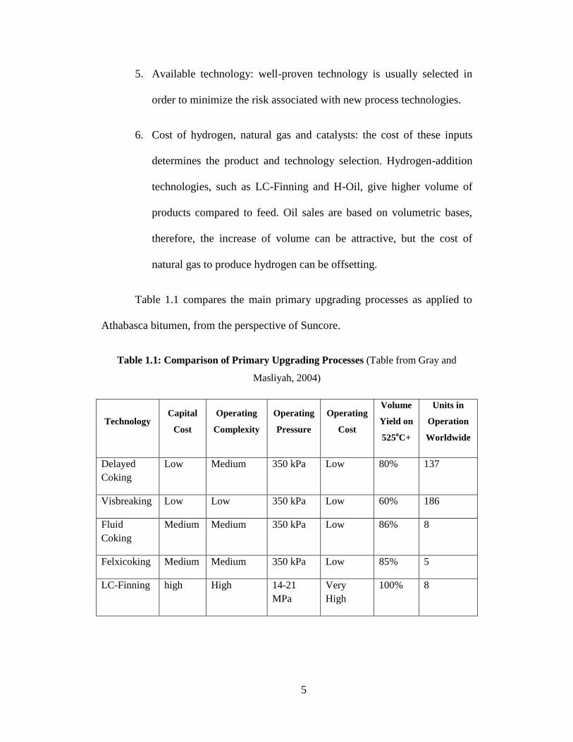
Table 1.1 compares the main primary upgrading processes as applied to
Athabasca bitumen, from the perspective of Suncore.
Table 1.1: Comparison of Primary Upgrading Processes (Table from Gray and
Masliyah, 2004)
Technology Capital
Cost
Operating
Complexity
Operating
Pressure
Operating
Cost
Volume
Yield on
525oC+
Units in
Operation
Worldwide
Delayed
Coking
Low Medium 350 kPa Low 80% 137
Visbreaking Low Low 350 kPa Low 60% 186
Fluid
Coking
Medium Medium 350 kPa Low 86% 8
Felxicoking Medium Medium 350 kPa Low 85% 5
LC-Finning high High 14-21
MPa
Very
High
100% 8

6
In current upgraders, coking is the most common choice for primary
upgrading. Coking is more appealing due to the lack of catalysts that can handle
the high solid and water content in mined bitumen without the high cost of
catalyst consumption. The most commonly used coking processes are delayed
coking and fluid coking. The delayed coking process is usually attractive when
there is no market for fuel oils. Delayed coking process has long reaction times in
the liquid phase, compared to fluid coking. The condensation reactions that lead
to production of high aromatic content coke product also tend to retain sulfur,
nitrogen and metals. Unlike the semi-batch delayed coking process, fluid coking
is a continuous operation that uses shorter reaction times in the liquid phase and
also uses higher temperature. The short residence times of the cracking products
in the liquid phase improves the products yield in fluid coking compared to
delayed coking. More detailed discussion on the different coking processes is
given in the following chapter.
1.3 Research Objectives
In fluid coking, the thermal cracking of heavy oil feed stocks occurs on the
surface of fluidized coke particle in the fluid coking reactor usually at 510-550oC.
Forming thin liquid layer on the surface of coke particles is very important in
order to ensure maximum heat transfer from the hot coke particle to the reacting
liquid film and to minimize the trapping of the reaction products within the liquid
due to mass transfer resistance.
Different studies on cold systems (House et al., 2004, McMillan et al.,
2005, McDougal et al., 2005, House et al., 2008 and Weber et al., 2008), pilot

7
studies and solid products analysis (Gray 2002) indicated that liquid feeds tend to
form agglomerates with the solid particles. Evidence from industrial reactors also
shows that during the coking process the solid coke particles and the heavy oil
feed tend to form solid-liquid agglomerates. These agglomerates then survive and
travel within the reactor to cause operational problems such as fouling of the
reactor internals and potentially defluidization of the fluidized bed. Also, when
the reacting liquid is trapped in the agglomerates it tends to undergo undesired
condensation and polymerization reactions that increases the coke yield and hence
decreases the yield of the desired distillable products.
The objectives of this research are
To determine the effect of different variables on the yield of coke from
AVR-solid agglomerates, such as agglomerates size, liquid
concentration, reaction temperature and heating rate.
To study the behavior of the AVR-solid agglomerates and measure
their temperature profile under controlled conditions.
1.4 Research Approach
To achieve the objectives of the research, two different types of reactors
were used to conduct the experiments on the AVR-solids agglomerates; induction
furnace reactor and fluidized bed reactor.
In the induction furnace reactor the AVR-coke agglomerates were reacted
under controlled conditions by placing the agglomerates between two Curie-point
alloys and placing them in an induction coil to heat up the Curie-point alloys to

8
their Curie-point temperature rapidly. The induction furnace experiments were
done under 100% survival conditions, i.e. the agglomerates stayed intact through
the experiments without disintegration. The coke yield in the agglomerates were
measured based on the amount of coke formed after the reaction relative to the
amount of AVR in the unreacted agglomerate. The induction furnace reactor was
also used to determine the coke yield in reacting AVR thin films by spraying the
AVR directly on the Curie-point strips and running the AVR-covered strips in the
induction coil. The results from the agglomerates and the thin films reaction were
compared to determine the effect of agglomeration on coke yield. Agglomerates
of different thicknesses and diffetent AVR concentration were also tested to study
the effect of the different agglomerates varaiables on coke yield. Also, the
temperature profile within the agglomerates was measured during the heating time
and a mathematical model was made to describe the change of temperature with
time.
In the fluidized bed reactor, AVR-silica agglomerates were reacted in a
fluidized bed of silica. Silica was used instead of coke in making the agglomerates
and as fluidization solids in order to be able to determine the amount of coke
formed after the reaction by burning the fluidized bed content and determine the
coke formed by absorbing the CO2 in alkaline solution. Due to fluidization, the
survival conditions of the fluidized bed experiments were less than 100%, that
gave the chance to study the effect of agglomerates disintegration on the coke
yield by comparing the fluidized bed results to the induction furnace results.
Similar to the induction furnace experiments, agglomerates with different sizes

9
and different AVR content were reacted to study the effect of these variables on
the coke yield.
1.5 Thesis Outline
In the next chapter, the background literature on the upgrading of heavy
oil generally and fluid coking particularly is reviewed. The background literature
also covers the coking kinetics and formation of agglomerates. Chapter 3 deals
with the materials and experimental methods used in the study. The results from
the experimental work are then presented in chapter 4 and the experimental results
then discussed in chapter 5. Finally, chapter 6 includes the conclusions.

10
2 LITERATURE REVIEW
2.1 Heavy Oil and Bitumen
Oil sands are unconsolidated sand deposits that are impregnated with high
molar mass, highly viscous petroleum fluid. Bitumen production from oil sands is
achieved either by in-situ operations for the deposits located deeper than 75 m
below the ground, or by surface mining for shallower deposits. In 2007, the oil
production from Alberta oil sands was estimated at 1.25 million barrels
(Government of Alberta, 2009). Compared to conventional crude oil, bitumen
properties are less favorable due to low API gravity, high content of vacuum
residue, sulfur, nitrogen, metals and high viscosity. Table 2.1 shows a comparison
of some properties of Athabasca bitumen and crude oil. (Speight, 2007)
Bitumen and heavy oil are differentiated according to their properties
according the following definitions:
Bitumen : APIo<10, ρ>1000 kg/m
3, µ>10
5 mPa.s at 15
oC
Heavy Oil: 10<APIo<26, ρ<1000 kg/m
3, µ10
2-10
5 mPa.s at 15
oC

11
Table 2.1: Properties of Athabasca bitumen and Crude oil (Speight, 2007)
Property Athabasca Bitumen Crude Oil
Specific gravity 1.03 0.85–0.90
Viscosity (cp)
38oC-100
oF 750,000 <200
100oC-212
oF 11,300
Pour point (oF) >50 ca. -20
Elemental analysis (wt.%)
Carbon 83.0 86.0
Hydrogen 10.6 13.5
Nitrogen 0.5 0.2
Oxygen 0.9 <0.5
Sulfur 4.9 <2.0
Ash 0.8 0.0
Nickel (ppm) 250 <10.0
Vanadium (ppm) 100 <10.0
Fractional composition (wt.%)
Asphaltenes (pentane) 17.0 <10.0
Resins 34.0 <20.0
Aromatics 34.0 >30.0
Saturates 15.0 >30.0
Carbon residue (wt.%)
(Conradson carbon
residue)
14.0 <10.0

12
2.2 Thermal Cracking and Coking Processes
The residue fraction (524oC+ fraction) of bitumen and heavy oil needs to
be processed in upgraders, and converted into distillable products. Bitumen from
oil sands is upgraded to produce high quality synthetic oil comparable to the
conventional light sweet crude, to produce pipelineable liquids with little or no
diluents, or to produce cracked products with no vacuum residue. The choice of
upgrading technology depends on the properties of feed material and the targeted
markets. Upgrading processes either involve disproportionation of the feed into
light ends, liquid products and solid byproduct (coke) as in coking processes, or
catalytic hydrogen addition, such as LC-Finning or H-Oil processes. Thermal
cracking processes are usually followed by hydroprocessing of the cracked
products, either at the upgrader site or at a downstream refinery, to increase their
quality and remove heteroatoms, such as nitrogen and sulfur. The industrial
thermal cracking and coking processes are reviewed in this section.
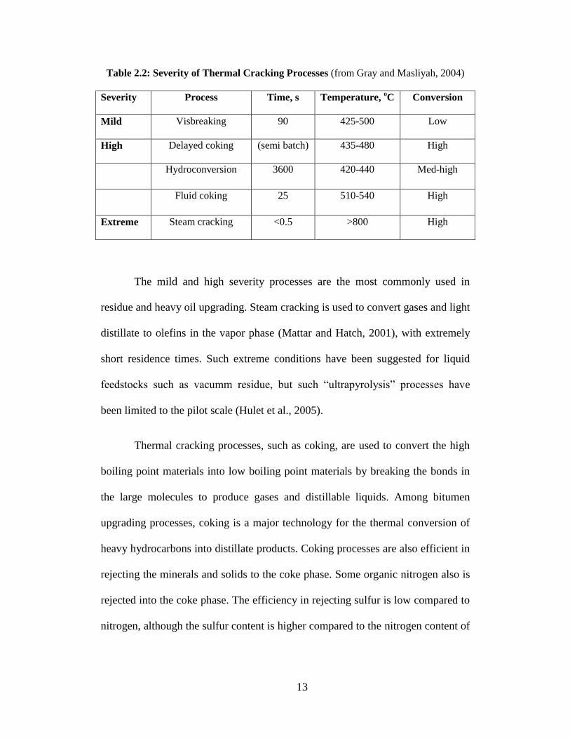
The severity of thermal cracking processes determines the conversion and
the products characteristics. Table 2.2 shows the severity of the different cracking
processes and the corresponding conversions
13
Table 2.2: Severity of Thermal Cracking Processes (from Gray and Masliyah, 2004)
Severity Process Time, s Temperature, oC Conversion
Mild Visbreaking 90 425-500 Low
High Delayed coking (semi batch) 435-480 High
Hydroconversion 3600 420-440 Med-high
Fluid coking 25 510-540 High
Extreme Steam cracking <0.5 >800 High
The mild and high severity processes are the most commonly used in
residue and heavy oil upgrading. Steam cracking is used to convert gases and light
distillate to olefins in the vapor phase (Mattar and Hatch, 2001), with extremely
short residence times. Such extreme conditions have been suggested for liquid
feedstocks such as vacumm residue, but such “ultrapyrolysis” processes have
been limited to the pilot scale (Hulet et al., 2005).
Thermal cracking processes, such as coking, are used to convert the high
boiling point materials into low boiling point materials by breaking the bonds in
the large molecules to produce gases and distillable liquids. Among bitumen
upgrading processes, coking is a major technology for the thermal conversion of
heavy hydrocarbons into distillate products. Coking processes are also efficient in
rejecting the minerals and solids to the coke phase. Some organic nitrogen also is
rejected into the coke phase. The efficiency in rejecting sulfur is low compared to
nitrogen, although the sulfur content is higher compared to the nitrogen content of

14
the feed materials. Table 2.3 shows the representative compositions of Athabasca
feed and the corresponding compositions of delayed and fluid coke.
Table 2.3: Representative compositions of Athabasca feed and delayed and
fluid coke (Data from Gray, 1994 and Chung et al., 1996)
Component Feed Delayed coke Fluid coke
Carbon, wt% 84.22 83.54 83.47
Hydrogen, wt% 10.23 4.43 1.77
Sulfur, wt% 5.1 6.72 6.52
Nitrogen, wt% 0.45 1.60 2.03
H/C 1.46 0.64 0.25
2.2.1 Delayed Coking
Delayed coking is a semi-batch process that is the most widely used
method for conversion of vacuum residues from bitumen, heavy oil, and
conventional petroleum. The process unit consists of at least two coking vessels
and a coker fractionator (Figure 2.1). In the process represented in figure 2.1, the
feed is injected at the bottom of the fractionator where it is preheated and any
light fractions are allowed to vaporize. The feed, along with the bottom product
from the fractionator, is heated to about 500oC in a heater then introduced to the
bottom of the coking vessel (coke drum). The gases and distillates are withdrawn
from the top of the coking drum and quenched by colder oil in the coker
fractionator. The coke is deposited in the coke drum, beginning at the bottom,

15
until the drum is full. When one of the coking drums becomes full, the feed is
switched to the other coking drum and the coke is removed from the first drum. A
typical cycle of delayed coker usually takes 48 hours. The common operating
problems in delayed coking include foaming in the drum, shot coke formation,
coke deposition in heater tube and fouling of the fractionator. Shot coke can be a
safety hazard during the quenching of the coke with water, it can break open and
propelled by steam when water hit the hot center. Shot coke formation can be
suppressed by ensuring that gas oil components are present to act as a solvent,
therefore, high pressure, more recycle and lower temperature help the suppress
shot coke.
2.2.1.1 Eureka Process
The Eureka process was invented by Kureha Chemical and Chiyoda of
Japan (Aiba et al., 1981). The process is similar to the delayed coking process.
Instead of coke as a byproduct, Eureka gives a high density liquid pitch. Steam is
used to strip the volatile liquid product and extend the coking induction period.
The same concept of a semi-batch process, using two alternating reactors, is
applied in the process. While one of the drums is being filled with the reacting
pitch the other drum is getting emptied. The pitch from the process is conveyed
and cooled to solidify then flaked, or it can be used as boiler fuel. Compared to
delayed coking, Eureka gives lower yield of gases and higher yield of liquids and
lower yield of pitch (Wiehe, 2008, Speight, 2007).

16
Figure 2.1: Schematic flow diagram of delayed coking process (PROCESS
CHEMISTRY OF PETROLEUM MACROMOLECULES by I. A. Wiehe.
Copyright 2008 by TAYLOR & FRANCIS GROUP LLC - BOOKS. Reproduced
with permission of TAYLOR & FRANCIS GROUP LLC - BOOKS in the format
Dissertation via Copyright Clearance Center)

17
2.2.2 Fluid Coking
Fluid coking is a continuous process that was developed by Exxon in the
1950’s (Voorhies and Martin, 1953). In fluid coking (Figure 2.2), the heavy feed
of bitumen is sprayed through steam-assisted atomizing nozzles into a fluidized
bed of hot coke particles. Coking occurs on the surface of these particles at
temperature of 510-550oC, where the liquid reacts and thermally cracks to give
gas oil, naphtha, LPG, dry gases (C1, C2) and coke byproduct. The cracked
vapors rise to the top of the reactor, pass through cyclones to remove entrained
particles of coke, and enter the scrubber in the top portion of the vessel. There the
vapors are quenched by contact with condensed liquid of fresh feed. After
stripping the coke with steam to remove liquids at the bottom of the reactor, the
coke passes to the burner where a portion of the coke is burned to supply the heat
to the reactor. The yields of the products are determined by the feed properties,
the temperature of the bed and the residence time of the vapors in the reactor. The
residence time of vapor-phase products is smaller compared to delayed coking,
which reduces polymerization and coking reactions. Also, the excellent heat
transfer in the fluid bed allows the reactor to operate at higher temperature, giving
more cracking of volatiles from the coke. The higher operating temperature of
fluid coking results in higher yield of liquid products but with lower quality
compared to delayed coking. These factors generally give a lower yield of coke
from fluid bed operation than from delayed coking, and the yield of gas oil and
olefins is increased. (Gray, 1994). Fluid coking produces ca. 1.2 CCR (Conradson
Carbon Residue; an experimental method presented by Conradson, 1912, to

18
determine the carbonaceous residue formed after thermal destruction of a sample)
of which about 20% is burned in the heater, while delayed coking produces about
1.4-1.6 CCR coke (Wiehe, 2008).
2.2.3 Flexi Coking
Flexi coking is another continuous coking process and is considered a
direct descendent from the fluid coking process. Flexi coking process has a
similar configuration as fluid coking, with the addition of a gasifier in which the
excess coke is gasified to produce fuel gas (Figure 2.3). Coke is gasified using
steam and air at temperatures of 830-1000oC. The heater in flexi coking is placed
between the gasifier and the reactor and used to transfer heat between the two
vessels.
The common problems in fluid coking and flexi coking are the fouling of
reactor internals, over cracking of liquid products, fractionator fouling,
defluidization of the bed or “bogging” that happens due to agglomeration of coke
particles, and fouling in the burner if too much hydrocarbons is carried over with
coke.

19
Figure 2.2: Schematic flow diagram of fluid coking (PROCESS CHEMISTRY
OF PETROLEUM MACROMOLECULES by I. A. Wiehe. Copyright 2008 by
TAYLOR & FRANCIS GROUP LLC - BOOKS. Reproduced with permission of
TAYLOR & FRANCIS GROUP LLC - BOOKS in the format Dissertation via
Copyright Clearance Center)

20
Figure 2.3: Schematic flow diagram of Flexi coking process (PROCESS
CHEMISTRY OF PETROLEUM MACROMOLECULES by I. A. Wiehe.
Copyright 2008 by TAYLOR & FRANCIS GROUP LLC - BOOKS. Reproduced
with permission of TAYLOR & FRANCIS GROUP LLC - BOOKS in the format
Dissertation via Copyright Clearance Center)

21
2.2.4 Other Coking Technologies
Beside the most common coking processes mentioned above, other coking
processes have been proposed and developed to suit heavy oil processing. The
concept of each of these processes is closely related to the older processes. All
coking processes depend on a heat source that supplies the heat for the thermal
cracking reaction. This heat source could be either a furnace or heater like the
delayed coking process, or hot solids (coke or sand particles) like the case of fluid
coking and flexi coking. The method of delivering and moving the solids around
the system is a key difference between the processes. Some of these processes are
still under development and testing in pilot scales and other processes have been
discontinued after reaching certain level of development in lab, pilot or
commercial scale.
2.2.4.1 Ivanhoe Heavy to Liquid (HTL) Process
The origins of the HTL process are technology initially developed by
Ensyn Group in the early 1980s for biomass conversion (Veith, 2006, Koshka et
al., 2008). The HTL process uses a short residence time for reaction in a
continuous process. The process concept is similar to fluid coking, except that the
heavy oil feed is mixed with hot circulating silica instead of coke particles. Coke
is deposited on the silica particles during the thermal cracking reaction. The coke
covered silica and the vapor products are separated in cyclone system, then the
vapors are quenched rapidly and condensed. The condensed products either
directed to a product tank for blending, or are recovered in a distillation column

22
for further separation. Part of the non-condensable gas is recycled to the reactor
and can be used as fluidization gas.
The coke covered silica is directed to fluidized bed reheater where all of
the coke is burnt to heat the silica particles, which are recycled to the reactor. The
heat from coke combustion can be used to generate high pressure steam for
electricity or in situ production. A pilot plant that was built by Ensyn was used to
test the process for heavy oil upgrading. In 2004 a 1000 bbl/day commercial
demonstration plant was initiated in the Belridge Heavy Oil Field in southern
California (Veith, 2006). Commercial scale of operation is expected to be in the
range of 10,000 to 15,000 bbl/day (Oilsands Review, 2007).
2.2.4.2 ETX Systems Upgrading Process
The ETX cross flow reactor was developed by Envision Technologies
(Brown et al., 2006), as an improvement on the fluid coking process. In the ETX
reactor, the moving hot solid particles (coke or sand) are introduced to the reactor
and the feed of heavy oil is sprayed onto the particles, where the thermal cracking
reactions take place. The fluidized solids move in the horizontal direction from
one end of the reactor to the other. Fluidization gas is introduced from the bottom
of the reactor and in the vertical direction, perpendicular to the direction of solid
movement. The vapor products are swept by the fluidization gas and collected
from the top of the reactor. The cross flow design of the reactor decoupled the
residence times of the moving solid particles and the vapor phase. The solids will
have enough time to move through the reactor for complete conversion of the
liquid feed on the solids and the vapor products are collected and quenched
23
rapidly to stop any further cracking reaction in the vapor phase. The coke-covered
solids are collected at the end of the reactor and send to the burner where the coke
is combusted to reheat the solids and produce steam. The ETX process is
currently operated on a one bbl/day pilot unit in the National Centre of Upgrading
Technology (NCUT) (Oilsands Review, 2007 and ETX Systems, 2009).
2.2.4.3 ART Process
The ART process was developed by Engelhard Corp. (Bartholic, 1981).
The main objective of the ART process was to upgrade the heavy oil feedstock to
meet the fluid catalytic cracking (FCC) requirements by rejecting metals, nitrogen
and carbon. The ART process used inexpensive microporous solids in a fluidized
bed as a heat source and coke collection surface. Coke yield in the ART process
was less than the CCR content of the feed, and most of the liquid product was in
the atmospheric residue boiling range needed for FCC. The solids from the coker
were burned in a burner to remove the formed coke and circulated to the reactor.
Fouling was a major problem in the ART process due to unconverted feed on the
solids particles and polymerization of olefins. The process was commercially
operated at an Ashland Petroleum Refinery using a revamped FCC unit, but it was
plagued by fouling problems and was eventually shut down (Wiehe, 2008)
2.2.4.4 Fluid Thermal Cracking (FTC) Process
The FTC process was invented by Fuji Standard Research (Miyauchi et
al., 1988). In FTC the heavy feed was cracked in a fluidized bed of porous solids
to produce distillate and coke and the produced coke was gasified to produce fuel
gas. The feed was injected to the reactor and absorbed into the pores of the solid

24
particles by the capillary forces. The thermal cracking took place in the pores and
the surface of the solid particles was kept dry which maintained good fluidity in
the reactor (Speight, 2007). The solid particles with the formed coke were sent to
the gasifier, where coke was gasified and fuel gas was produced. Fluidization gas
that contained hydrogen was used in the reactor, which reduced coke formation
due to the presence of hydrogen. The dilution of hydrogen by the generated light
ends caused a problem in hydrogen stream recycle. The FTC process was only
operated in a three bbl/day pilot (Wiehe, 2008)
2.2.4.5 Chattanooga Process
Chattanooga process was developed by Chattanooga Corp. to directly
convert unconventional oil resources, such as oil sands, oil shale or in-situ
bitumen, to synthetic crude oil (Chattanooga Corp, 2010). The process uses fluid
bed reactor and associated fired hydrogen heater. Hydrogen, heated in the fired
heater, is used as a heat carrier to the reactor, reactor fluidization gas and a
reactant. The particulate solids are separated from the reactor overhead gases then
the hydrocarbons are condensed and separated from the gases stream. Hydrogen
and light hydrocarbons are separated from acid gases in an amine unite before
being mixed with makeup hydrogen and being recycled to the fired heater. The
reaction kinetics of Chattanooga process were proven in a pilot plant at the
National Centre of Upgrading Technology (NCUT) in Devon, Alberta, Canada.
Another pilot plant testing achieved fluidization and extracted 100% of Colorado
oil shale. Pilot plant studies also demonstrated production of 28-30 oAPI product
25
from oil sands. Chattanooga Crop is preparing to design, construct and operate a
demonstration facility as a next step in the commercialization of the process.
2.2.4.6 Discriminatory Destructive Distillation (3D) Process
The 3D process was invented by Bartholic (Bartholic, 1989) and became a
joint venture of Bartholic and Coastal (Bar-Co) and was demonstrated over six
month period at a refinery (Wiehe, 2008). 3D process used coke as a heat source.
In the 3D process the feed was sprayed into a curtain of falling hot coke particles.
The 3D gave a very short residence time of the vapors to minimize the secondary
cracking reactions. The solids with incompletely converted feed fell off to a fluid
bed with higher residence time (similar to fluid coker) to complete the cracking
reactions (Bartholic, 1989). The process was eventually shut down due to some
operational problems with the longest run being six weeks.
2.2.4.7 LR-Flash Coker
LR- Flash process was developed by Lurgi. In the LR-Flash, the reactor is
a mechanical screw that gives good mixing and plug flow of the hot solids and
heavy oil feed. Sand or coke can be used as the solid phase in the reactor. This
process has short residence time of the vapor products to prevent over cracking
(Wiehe, 2008). The solid with formed coke are burned to provide the heat for
reaction. The LR-Flash has limitation with respect to size, its relatively small
capacity limits its use with high capacity refineries. Because this process uses
mechanical screw reactor to mix hot solids with feed material, it is suitable for
high solid content feed, or feed with poor flow properties. This process was
operated in lab, pilot and commercial scale. The commercial scale, known as

26
SATCON, was operated at Exxon Ingolstadt refinery in Germany and was shut
down due to fouling problems.
2.3 Coke Formation and Coking Kinetics
2.3.1 Fundamentals of Residue Cracking
Cracking is a decomposition of the residue fractions to convert high
molecular weight compounds to lower molecular weight products. Thermal
cracking is a non-catalytic process that takes place at commercially useful rates at
high temperatures of over 410oC.
Cracking of high molecular weight products is achieved by breaking the
chemical bonds in cracking reactions. In residue cracking, the targeted bonds are
the carbon-carbon and carbon-sulfur bonds. The difficulty in breaking the
chemical bonds depends on the structure of the compound. The following table
gives the bond dissociation energies for different bonds in bitumen compounds.
Table 2.4: Bond Dissociation Energies (Benson, 1976)
Chemical Bond Energy, kJ/mol Energy, kcal/mol
C-C (aliphatic) 355.9 85
C-H (n-alkanes) 410.3 98
C-H (aromatic) 462.6 110.5
C-S 322.4 77
C-N (amines) 351.7 84
C-O (methoxy) 343.3 82

27
Thermal cracking is a free radical chain reaction. The thermal cracking
reactions start with initiation step, where the carbon-carbon bond scission occurs
to form free radicals. The free radicals react by abstracting a hydrogen atom from
hydrocarbon or undergoing further cracking to produce stable product and a new
free radical. Cracking usually occurs at bonds β to the carbon atom that carries the
unpaired electron. The following is an example of chain reaction of n-alkane
cracking (Blanchard and Gray, 1997).
Initiation **
ji RRM (2.1)
Hydrogen transfer *
1
*
1 MHRMR (2.2)
Β-scission OlefinnRM *
2
* (2.3)
22
*
2
* CHCHnRR ii (2.4)
Isomerization **
sp RR (2.5)
Termination productsRR ji ** (2.6)
Where M and M* are the parent alkane and the parent radical, R1
* and R1H
are the methyl or ethyl radical and the corresponding alkane, R2* is the methyl,
ethyl or higher primary alkyl radical, Ri* is the butyl or higher radical and Rp
* and
Rs* are the primary and secondary pentyl or higher radicals.
The cleavage of the carbon-carbon bond requires a high activation energy,
from the bond dissociation energy, 356 kJ/mol (85 kcal/mol) in the case of the
aliphatic C-C bond (see table 2.4). On the other hand, propagation steps have

28
much lower energy requirement. The β-scission reaction has activation energy of
125-146 kJ/mol, while hydrogen abstraction has activation energy of 46-71
kJ/mol (Blanchard and Gray, 1997). The free radicals are presented in very low
concentrations, but they participate in the chain reaction many times to give
significant amounts of cracked products per mole of initiation reaction.
The activation energy for cracking of bitumen is comparable to the overall
activation energy for cracking on n-alkanes. Wiehe (2008) reported activation
energy values of 213.18 kJ/mol (50.9 kcal/mol) for Cold Lake short path
distillation bottoms.
2.3.2 Mechanism of Coke Formation
Coke can be defined as a carbonaceous solid that is formed from the
calcination of carbon-rich materials. In petroleum processing the term coke is
commonly used as a solubility term to describe the toluene-insoluble material.
Coke is formed as a separate phase during thermal cracking processes. In coking
processes, coke formation is part of the design and is targeted increase the H/C
ratio in the liquid products. On the other hand, coke formation is not desirable in
the hydroconversion and hydrotreating processes.
Coke forming tendency is an important parameter for upgrading. It is
measured by pyrolyzing sample of the heavy oil under controlled conditions in
absence of oxygen and determined as the amount of solids formed after the
pyrolysis as a fraction of the initial sample weight. The coke forming tendency is
usually measured as Conradson Carbon Residue (CCR), Rambsbottom Carbon

29
Residue (RCR), or Micro Carbon Residue (MCR). All three methods use the same
concept to determine the coke forming tendency with differences in the
equipment used and the heating conditions. The Conradson method (ASTM D-
189) measures carbon residue by evaporative and destructive distillation. The
sample is placed and heated in a sample dish until vapor ceases to burn and no
blue smoke is observed. The sample dish is weighted after cooling and the carbon
reside is calculated as a percent of the original sample weight. The Ramsbottom
test (ASTM D-524) uses 4 grams of the sample in a glass bulb then inserting the
bulb in a heated bath for 20 minutes. The bath temperature is maintained at 553
oC. after the test the bulb is weighted and the carbon residue is determined. The
micro carbon residue method (ATSM D-5430) uses an analytical instrument to
measure Conradson carbon in an automated set.
Wiehe (1993 and 2008) suggested that the coke formation during the
thermal cracking of heavy residue occurs by a mechanism that involves the liquid-
liquid phase separation of reacted asphaltenes to form a phase that is lean in
abstractable hydrogen. Wiehe observed a coke induction period before coke starts
to form. During this period, the asphaltene concentration increases and reaches a
maximum then decreases. The maximum occurs at the same reaction time as the
end of coke induction period (Figure 2.4). The duration of the induction period
depends on the feedstock and the coking temperature. At lower coking
temperature the induction period is long and starts to shorten with increasing the
temperature and even disappear at high temperatures. This phenomenon is used in
the design and operation of the industrial coking processes to prevent formation of

30
coke in undesired areas, such as heaters and distillation towers. Wiehe suggested
that asphaltenes reach a solubility limit in heptane soluble fraction before forming
coke. Wiehe (1992) proposed a phase diagram for coke formation behavior based
on hydrogen content and molecular weight, he observed that data for different
solubility fractions tend to cluster into distinct zones on a plot of molecular
weight versus hydrogen content (Figure 2.5)

31
Figure 2.4: Coke formation from three reactants: asphaltenes, full resid, and
heptane-soluble portion of resid for Cold Lake vacuum resid at 400oC
showing different coke induction periods (PROCESS CHEMISTRY OF
PETROLEUM MACROMOLECULES by I. A. Wiehe. Copyright 2008 by
TAYLOR & FRANCIS GROUP LLC - BOOKS. Reproduced with permission of
TAYLOR & FRANCIS GROUP LLC - BOOKS in the format Dissertation via
Copyright Clearance Center)

32
Figure 2.5: The solvent–residue phase diagram of eight different residues
and their thermal reaction products displays each of the five classes in
unique areas (PROCESS CHEMISTRY OF PETROLEUM
MACROMOLECULES by I. A. Wiehe. Copyright 2008 by TAYLOR &
FRANCIS GROUP LLC - BOOKS. Reproduced with permission of TAYLOR &
FRANCIS GROUP LLC - BOOKS in the format Dissertation via Copyright
Clearance Center)

33
Experimental observations showed that the toluene-insoluble solids that
form at cracking temperatures are not the friable precipitates that are recovered at
room temperature. During the heating of heavy oil, polymerization and
condensation reactions process rapidly with the liquid phase until the products of
the reactions remain no longer soluble and form a meso-phase that is different
than the toluene-insoluble solids. The meso-phase is a liquid-crystalline state
which shows the optical birefringence of disc-like nematic liquid crystals. It can
be formed as intermediate phase during the thermal cracking and can be observed
depending on the reactor conditions and feed properties. Wang et al. (1998)
observed that the toluene-insoluble fraction formed a liquid-oil emulsion at
reactor condition, consisting of toluene-insoluble sphere suspended in gas oil.
This observation suggested that the toluene-insoluble material was liquid or
plastic at reactor conditions, which agrees with the theory of liquid-liquid phase
separation as a step in coke formation.
Wiehe (2000) divided coke formation during thermal cracking into two
mechanisms: intrinsic and extrinsic. The intrinsic coke is formed from the large
aromatic molecules in the feed (5 rings or more). These large organic compounds
contain aromatic bonds that require very high dissociation energy in order to
crack. While the aromatic core is resistant to cracking, the side chains attached to
the aromatic core can be cracked to form lighter compounds, leaving the large
aromatic core to form coke. Because these large organic structures are very
difficult to crack, they must be rejected in order to increase the H/C ratio of the
processed feed, thus, the intrinsic coke can be considered the desirable amount of

34
coke that is formed or rejected to improve the quality of the products. The second
mechanism of coke formation is polymerization and recombination of lighter
fraction to form heavier compounds and is called extrinsic coke. The extrinsic
coke formation is considered undesirable because it comes on the expense of
losing some of the lighter compounds in the undesired coke formation reactions.
Figure 2.6 shows the different pathways of coke formation based on extrinsic and
intrinsic coke mechanism.
Dutta et al. (2001) directly measured the formation of the extrinsic type of
coke by labeling bitumen samples with 13
C isotope and tracing its appearance in
the products. They found that the amount of the tracer in the coke formed
increased with increasing the thickness of the reacting liquid films. The amount of
the extrinsic coke increased with increasing the length of the diffusion paths, and
consequently the mass transfer resistance, for the cracked products of the reaction
to escape from the liquid film. The longer the diffusion path, the higher the
chance for the cracked products to undergo the undesired recombination and
polymerization reactions. This observation lead to further investigation of the role
of mass transfer and its coupling with coking kinetics, as will be discussed later in
this chapter.

35
Figure 2.6: Intrinsic and extrinsic coke formation mechanism (PROCESS
CHEMISTRY OF PETROLEUM MACROMOLECULES by I. A. Wiehe.
Copyright 2008 by TAYLOR & FRANCIS GROUP LLC - BOOKS. Reproduced
with permission of TAYLOR & FRANCIS GROUP LLC - BOOKS in the format
Dissertation via Copyright Clearance Center)

36
2.3.3 Coking Reaction Kinetics
In case of vacuum residue processing, the reacting and product mixtures
have huge numbers of components present, which complicate the reaction and
kinetic modeling. Increasing the number of components in any reaction means
increasing the kinetic parameters that have to be estimated and, consequently,
increasing the experimental data required for parameter estimation which makes
modeling the individual components in mixtures during reactions becomes nearly
impossible. Besides that, the analytical methods for defining the component
concentrations and chemical structure for vacuum residue are not available. In
order to model the process, the oil mixtures are divided into lumps and each lump
is assumed to behave as an independent entity. This lumped system would
accurately describe the behavior the parent more complex system. (Wei and Kuo,
1969; Kuo and Wei, 1969; Ancheyta, 2005). Almost all the work done to date
employed lumped kinetics with different approaches to seek a better fit to the
experimental data and actual process.
In the kinetic model for coke formation based on phase separation, Wiehe
(1993) presented the conversion of asphaltene over the whole reaction range and
conversion of heptane-soluble during the coke induction period as first order
reactions. The asphaltenes have maximum solubility in the heptane soluble phase,
when this solubility limit is reached the insoluble product asphaltenes is converted
to coke and heptane soluble byproduct.
The kinetic model proposed by Wiehe was as follows:

37
)11.2(1
)10.2(
)9.2(
)8.2(1
)7.2(1
**
*
max
**
**
max
**
*
yHTIyA
AAA
HHSA
VnmnHmAA
VaaAH
ex
ex
L
k
k
A
H
Where a, m and n are stoichometric coefficients; A+ is reactant
asphaltenes; A* is asphaltene cores; A
*max is maximum asphaltene cores that can
be held in solution; A*
ex is excess asphaltene cores beyond that can be held in
solution; H+ is reactant non volatile heptane soluble; H
* is product non volatile
heptane soluble; SL is solubility limit; TI is toluene insoluble coke; and V is
volatiles.
The model provided by Wiehe was shown to qualitatively describe the
experimental data for Cold Lake vacuum residue at 400 oC. The model used the
hypothesis that the phase separation occurs due to the incompatibility of the new-
formed phase with the oil phase, which attributes to the coke formation. This
hypothesis does not agree with the results of Gray et al. (2003), who found
insignificant amount of polynuclear tracers in the toluene insoluble coke phase,
which suggested that the oligomerization reactions that increase the coke phase
molecular weight has a major role in coke formation.
Rahmani et al. (2002 and 2003) studied the coking kinetics of asphaltenes
along with solvent interaction and chemical structure effects. They extended the
phase separation model proposed by Wiehe (1993) to the case of closed batch
reactor systems, as in the closed reactors the cracked products remain inside the

38
reactor with most of the heptane-soluble phase in the liquid phase, and to account
for the solvent interaction with asphaltenes. They also used a finite rate constant
for the formation of coke, kC (Equation 2.16) instead of the infinite rate constant
used by Wiehe (1993) in the TI formation reaction (Equation 2.11).
To account for the hydrogen acceptance ability of asphaltene, the phase
separation model was further extended by Rahmani et al. (2002 and 2003). The
asphaltene fraction was assumed to consist of unreacted asphaltenes with attached
side groups (A+), and two types of aromatic cores formed by cracking of the
initial asphaltenes, each with different hydrogen-accepting capability. Cores that
can accept enough hydrogen to change their solubility characteristics (A*A
) and
cores that cannot accept hydrogen (A*NA
). The cores that accepted sufficient
hydrogen from a donor were assumed to be converted to heptane-soluble material.
The modified model was as follows
)16.2(
)15.2(
)14.2(
)13.2(
)12.2(1
*
*
max
***
**
max
**
***
TIA
AAAA
VHSSA
solventdonorhydrogenofcaseinHA
VHcdAAdcA
C
A
k
ex
ANA
ex
L
kA
ANAk
The two fitting parameters, asphaltene cracking rate constant (kA) and
stoichometric coefficient (c), were found to correlate with two chemical
properties: sulfide content and aromaticity of the asphaltenes, respectively. The
kinetic model was shown to predict coke formation, based on the chemical
composition of other feed asphaltenes that were not used in model parameter
estimation.

39
Del Bianco et al. (1993) studied the kinetics of thermal cracking for the
residua at different temperatures. They assumed that the reaction pathway for
coke formation could not be represented by simple first-order kinetics due to the
non-linear correlation between the distillate and coke yields. They also found that
coke formation showed an induction period, which decreases as temperature
increases. Taking these observations into account, and instead of adopting the
solubility limit idea proposed by Wiehe (1993), they proposed a reaction scheme
with reaction intermediates.
DVRk 1' (2.17)
CIRVkk 32 (2.18)
Where I is the reaction intermediate in the coke production, VR’ is the
fraction of vacuum residue not converted VR=VR’+I, D is the distillates, C is
coke, and k1, k2 and k3 are the rate constants.
The condensation reaction, which is responsible for the coke formation,
was found to have higher activation energy; consequently, this reaction becomes
relatively more important as temperature increases.
The experimental results of Del Bianco et al. (1993) showed that the
disappearance of asphaltenes coincides with coke production. However, at high
severity, the coke yields exceed the initial amount of asphaltenes and therefore the
polymerization reactions also involve oil components. This result was confirmed

40
by experiments of deasphalted vacuum residue that gave 10.9% coke yield
compared to 29.7% coke in case of the whole vacuum residue at the same
conditions. When they examined the molecular parameters, such as H/C ratio,
number of carbon per alkyl side chain, aromatic carbon and unsubstituted
aromatic carbon, the results showed that the dehydrogenation of asphaltenes is a
consequence of the decrease of alkyl chain length and dealkylation reactions; both
processes cause the increase of aromaticity. Their explanation of the results was
that all of these reactions cause the progressive insolubilization of the aromatic
asphaltenes sheets and hence lead to the condensation reactions which give rise to
the appearance of mesophase and therefore to coke deposition.
Other kinetic studies have been performed to study coking kinetics with
different approaches and at different conditions. Wang and Anthony (2003)
studied the thermal cracking behavior of asphaltenes with a three-lump model.
They showed that an empirical relation of coke formation and asphaltenes
conversion gave a reasonable description of the kinetic behavior at high
conversion. Takatsuka et al., (1989) used the atmospheric equivalent boiling point
in determining the Arrhenius parameters and to describe the effect of phase
equilibrium in the reactor. Their model predicted the performance of different
types of reactor by taking the residence time distribution in consideration. The
residence time distribution was used to determine the average residence time in
the reactors in order to achieve complete conversion. They observed the degree of
reaction by the value of the softening point of pitch when pitch was the residual
product. The softening point of pitch was predicted as a function of residual

41
components and increased with the reaction time. Banerjee et al. (1986) studied
the kinetics of bitumen and its fractions (asphaltenes, soft resin, hard resin,
aromatics and saturates) in the temperature range from 395 to 510 oC. They found
that the rate of coke formation is higher for higher degree of aromaticity in the
feedstock. They proposed a reaction scheme but did not provide information
about the estimation of kinetic parameters.
42
2.3.4 Coupling of Mass Transfer with Reaction
Fluid coking usually has lower coke yield than the delayed coking
(Nelson, 1958; Speight, 2007). One of the fundamental differences between the
two modes of coking is the thickness of the reacting liquid phase. In fluid coking
the reacting phase is a thin film of bitumen over the hot coke particles, unlike the
delayed coking in which the reaction takes place in pool-like liquid phase. The
volatile cracking products have to diffuse through the liquid film in order to reach
the gas-liquid interface. In thicker films these compounds take longer time to
diffuse through the liquid film. As the reaction proceeds, the viscosity of the
liquid film increases (Aminu, 2004) and the diffusivity of the escaping products
decreases as the liquid phase transfers into a solid-like phase. These products will
be available in the liquid phase as free radicals or unsaturates for a certain period
and the longer the time they stay in the liquid phase the more likely they are to
recombine and to incorporate into coke.
Dutta et al. (2001) used 13
C labeled compound to track the pathways of
potential distillate compounds during cracking of the feed. They found that the
coke yield decreased with the reduction in the thickness of the liquid film. The
13C analysis showed a decrease in the
13C incorporation in coke fraction for both
heptane-soluble and heptane-insoluble tracers as film thickness was reduced from
150 to 15 . McCaffrey et al. (1998) observed bubble formation and film
deformation in cracking of vacuum residuum thin films. By performing the thin
film cracking on horizontal and angled surface, the coke yield was found to
increase with increasing the film thickness. Bubbles evolved slowly and a

43
formation of viscous layer on the reacting film trapped the bubble until the
pressure within the bubble increased sufficiently to deform the viscous layer.
Nagaishi et al (1998) compared TGA differential weight loss curves of bitumen at
different pressures. They observed a formation of a peak in the TGA differential
weight loss curve at atmospheric pressure. Another peak appeared at lower
temperature when the pressure was lowered to 0.4 kPa. This peak shifted to lower
temperatures and increased as the pressure was reduced. The shift with the low
temperature peak was consistent with the removal of volatile components of the
bitumen, which would distill of at lower temperatures as the pressure decreased.
Gray et al. (2001) studied the mass transfer role in reacting bitumen films
of thickness from 10 to 80 . The total coke yield and liquid MCR content
decreased with decreasing the liquid film thickness. For thick films, the final coke
product in the film indicated the occurrence of bubbling during the reaction, while
in thin films no evidence of bubbling was observed. They proposed a
mathematical model to describe the mass transfer phenomena with reaction,
which considers mass transport by diffusion and bubbling in thick films.
The mass balance equation was given by
)19.2(0)( *
12
2
PPBPPRP CCkCkCk
dx
CdD
Where CP and CR are the product and residue concentration, Cp*
is the
critical product concentration for bubble formation, and D is the diffusivity. The
rate constants are k1 for cracking of the residue to give products, kp for trapping of

44
the products in the liquid phase and kB is for transport of the products to gas-phase
bubbles.
Non-dimensionlization of the above equation gives
)20.2(022
2
2
dl
d
Where ψ is CP/CP*
and is Thiele modulus for thick films and has the
form
)21.2(2
2
D
Lkk BP
For the inner section of the film where the concentration of the gases is
higher than a critical concentration of bubble nucleation limit, and ` is the ratio
between the forward and retrograde reactions considering bubble formation.
For thin films the transport by bubbling does not occur, and the last term
in equation (2.19) can be dropped and the equation becomes
)22.2(012
2
PPRP CkCk
dx
CdD
And in dimensionless form
)23.2(022
2
2
dl
d
Where is Thiele modulus for thin films or the outer part of thick films,
where the gas concentration is below the nucleation limit

45
)24.2(2
2
D
LkP
And, is the ratio between the forward and retrograde reactions without
bubble formation.
In case of thick films, at large values of Thiele modulus the vapor products
are more likely to trapped and converted to coke, or to migrate to vapor bubbles,
than in the case of thin films. Lower values of Thiele modulus mean that the
liquid products will diffuse through the reacting liquid film rather than being
trapped or forming vapor bubbles. In case of reacting bitumen films, as the
reaction proceeds the viscosity of the liquid phase changes dramatically (Aminu
et al., 2004), which in turn decreases the diffusivity of the gas products and the
solution of the model equations becomes more complicated with variable Thiele
modulus.
At values of greater than unity, the rate of the cracking is higher than the
rate of trapping of the gas products in the liquid phase, and below unity the
trapping is dominant to the cracking reaction.
Gray et al. (2004) proposed a lumped kinetic model that included
cracking, coke formation and vaporization limited by vapor-liquid equilibrium
and mass transfer (Figure 2.7). The amount of extractable materials in the liquid
film did not follow first order kinetics, which also was described by the model
with an initial rapid devolatilization period followed by cracking. The model
suggested that the coke yield would decrease with increasing the reaction

46
temperature because of enhanced devolatilization. The authors suggested using
data from Aminu et al. (2004) to obtain better estimates of the liquid phase mass
transfer coefficient as a function of the conversion and using variable mass
transfer with time to enhance the agreement with the evolution of heavy oil
fraction data and to account for the insensitivity of the coke yield with
temperature.
Continuing on the work of Gray et al. (2004), Radmanesh et al. (2008)
revisited the kinetic model and provided a modified description of the mass
transfer limitation by correlating the diffusivity of the reaction products in the
reaction liquid film to the physical properties, which change greatly throughout
the reaction, and adopting the intrinsic and extrinsic coke formation mechanism
proposed by Wiehe (2000). The reaction scheme used by Radmanesh et al. (2008)
is shown in figure 2.8.
An understanding of the role of mass transfer in the coking reactions can
be employed to maximize the yield of distillate products and minimize the yield
of coke in the commercial reactors, by introducing thinner reacting liquid films. In
order to form a thin layer of the liquid feed over the coke particles, there must be
an efficient mechanism for distributing the feed on the coke in the fluid bed.
(Gray, 2002). The introduction of the liquid films to the fluidized bed can be
improved by optimizing process variables such as feed atomization, design of the
feed injection nozzle, the gas flow rate, and the reactor length to diameter ratio.
(Gray et al., 2001)

47
Figure 2.7: Schematic diagram of lumped reactions and volatilization during
coking in a thin film. Reactions are assumed to be first order. Rate constants
for reaction are ki, stoichometric yields are sij, and the mass transfer
coefficient is kGa. Equilibrium ratios are Ki (Gray et al., 2004)

48
1. Heavy Residue
(+650oC)
2. Light Residue
(524-650oC)
3. Gas oil
(343-524oC)
4. Distillates
(-343oC)
Intrinsic Coke
Extrinsic Coke
k1 S13 S12
S23
S14
kext
kint
S24 k2
Figure 2.8: Reaction network for thermal cracking of bitumen (Radmanesh et al.,
2008)

49
2.4 Bitumen Coke Agglomerates
2.4.1 Agglomerate Formation and Growth
Fluid coking uses finely divided coke particles as a heat carriers and
reaction surface. The mean particle distribution of coke particles is usually around
150 μm. Jet attrition nozzles are usually used to grind the coke particles to control
particle size and create fine seeds, and any oversized lumps are moved
periodically at the bottom of the reactor (Dunlop et al, 1958). The feed is
introduced to the reactor by steam-assisted spray nozzles. The droplet size of the
liquid feed is much larger than the coke particle sizes. Depending on the nozzle
design and the operation, the liquid feed droplet size can range from 300 μm to
3000 μm on average (Tollefson et al., 1997).
When the oil droplet enters the bed of a fluid coker, it comes into contact
with many coke particles, due to the difference in their sizes. Then those coke
particles accumulate with the liquid droplet and form a so called “gumball” (Gray
2002). McDougall et al. (2005) showed that viscosity and contact angle are the
two important criteria in agglomerates formation in fluid beds. Pilot studies and
analysis of solid particles from fluid-bed coking confirmed that the solid particles
and liquid feed tend to form agglomerates in the size range of 0.1 – 2 cm within
the bed of solid particles (Gray, 2002). The shear forces inside the bed due to the
bed velocity can pull the particles apart, also the cracking of the liquid and
devolatilization of the product can affect the strength of the gumball, specially
that the liquid has low initial viscosity (ca.1 cP) at the reaction condition and good
wetting ability what would give good spread of the liquid on the coke particles.

50
As the reaction proceeds the liquid viscosity increases very rapidly, while the
surface tension is not significantly affected, (Aminu et al., 2004). The volume of
liquid will decrease due to cracking and product evolution, which may lead to
increasing the internal cohesive forces and allow the agglomerate to survive in the
fluidized bed.
Another factor that has been studied and found to have significant effect
on agglomerate formation and solid liquid mixing in fluidized bed is the liquid
nozzle design. House et al. (2008) showed that improvements in the liquid-solid
contact in fluidized bed can be achieved by modifying existing nozzles and
developing new nozzle designs. By testing two types of nozzle designs and testing
the effect of modifying the design by using pulsation or adding an attachment to
the nozzle to enhance the solid entrainment, they showed the effect of nozzle
types on liquid solid mixing efficiency, agglomerate formation and agglomerate
size distribution. The enhanced solid entrainment (ESE) nozzle introduced by
McMillan et al. (2005) and House et al. (2004) showed improvement over the free
jet nozzle in solid-liquid mixing by increasing the amount of wetted solids and
achieving a more uniform primary solid-liquid mixture, which helps reduce
agglomeration in fluid beds.
Coke particles covered with a liquid layer, as well as the wet
agglomerates, circulate in the fluidized bed and the liquid reacts on the coke
surface with time. During the movement of wet coke particles and agglomerates,
they transfer the unreacted liquid to reactor internals causing fouling, especially in
the coke stripper section at the bottom of the fluidized reactor where

51
hydrocarbons are stripped using steam before coke exits the reactor (Bi et al.,
2005 and House et al., 2006). Fouling is a serious problem that can greatly affect
the operability of the fluid coking process. If the agglomerates keep forming and
growing, “bogging” or loss of fluidity of the bed can occur, because agglomerate
formation inside the bed increases the porosity of the bed, which in turn requires
increasing the minimum fluidization velocity (Ennis et al. 1991). Gray (2002)
showed that the required minimum fluidization velocity would increase in
proportion to the logarithm of the liquid film thickness. So, thin liquid films on
the coke particles in fluid coking can help reducing both the limitation of mass
transfer and defluidization, which reflects the role of good feed distribution on
both mass transfer and fluidization.
It has been shown that for a given collision velocity between the granules,
with thick enough liquid film and with high enough liquid viscosity, rebound of
the granules after collisions will be prevented and they will coalesce. Upon
collision of two particles with liquid film on their surface, the formed liquid
bridge helps binding the particles together. For the bridge to be stable, the kinetic
energy of the colliding particles must be dissipated by the viscous flow of the
liquid film. The balance between kinetic energy and viscous dissipation gives the
critical conditions for the formation of an agglomerated pair of particles
)25.2(ln1
10
*
L
L
eStv

52
Where e is the coefficient of restitution; L is the thickness of liquid layer;
L0 is the height of the asperities at the surface of the granule. (Ennis et al., 1991;
Keningley et al., 1997; Gray, 2002).
The viscous Stokes number of the system will be given by (Ennis et al.,
1991 and Keningley et al., 1997)
)26.2(9
)2(4 0
duSt D
v
Where D is the granule density; d is the granule diameter; 2u0 is the
relative velocity; and is the viscosity of the liquid.
In order for the granule to grow, this Stokes number must not exceed a
critical value. Collisions of particles with Stokes number higher than the critical
value does not result in stable liquid bridge. Ennis et al. (1991) observed three
granulation regimes based on the above two equations (2.25 and 2.26). For the
particles with Stv<St*
v, the rate of particles growth was independent on binder
viscosity and granule kinetic energy and critically depends on the presence and
distribution of binder. This is referred to as the non-inertial regime. In this regime,
the operating parameters such as spray drop size and spray distribution control the
growth of the granules. As granules grow, their Stokes number increases. When
the largest Stokes number reaches the critical value, granules kinetic energy and
binder viscosity start to play a rule. In this inertial regime, increasing binder
viscosity and decreasing granules kinetic energy will increase granule
coalescence. As the granule grow further and the average Stokes number reaches
53
the critical value, the distribution of Stv will be such that local regions where
Stv<St*v, where coalescence is possible, will be balanced with other regions of
disagglomeration where Stv>St*v, implying that in average granules growth is not
achieved. At the final regime when the growth of the granules was ceased all the
added binder coated the granules.
Minimum values for the liquid film thickness will help reduce the mass
transfer limitation, trapping of the cracked products and also prevent formation
and growth of agglomerate and defluidization by decreasing the value of critical
Stokes number, which the Stokes number of the particle must not exceed in order
to form stable liquid bridges and grow.
2.4.2 Agglomerates Disintegration and Breakage
Agglomerates can disintegrate by many mechanisms including internal
stresses caused by reaction and vapor evolution, external mechanical stress caused
by bed fluidization, and migration of liquid from the agglomerate to drier bed
particles (Weber et al., 2006). Agglomerate breakage is undesired in many
processes, but in fluid coking due to the aforementioned problems associated with
agglomerate formation, less agglomerate formation may be beneficial to the
coking reactions.
Agglomerates strength is affected by different factors some of them are:
(Verkoeijen et al., 2002)

54
The size and size distribution of the primary particles.
Agglomerate strength increases with decreasing the particle size
and for wider particle size distribution.
The porosity of the agglomerate, the strength increases with
decreasing porosity.
The binder surface tension. Agglomerate strength increases with
increasing the binder surface tension.
Most of the literature that investigated the agglomerate breakage and
disintegration deal with the mechanical impact mechanisms of breakage, like
when the agglomerates hit a stationary surface or when the agglomerate colloid,
which may be of some interest in case of the fluid coking. Almost no experiments
have been done to study the effect of vapor evolution on the agglomerate
breakage.
Agglomerates behavior inside the bed has different aspects and depends
on many variables and properties of both bed and agglomerate materials. Weber
et al. (2006) found that agglomerates of 9% moisture content tend to collect bed
materials and gain more weight than the lost binder weight while fluidization,
while the drier agglomerate do not. The drier agglomerate on the other hand
showed consistent erosion in a linear manner and that rate of erosion depended on
the solid particle size and particle size distribution in the agglomerates. They
found that the agglomerates that were made from hydrophobic materials did not
survive the fluidized bed, which supports the liquid binder role in making the
agglomerates, and those agglomerates have internal structure that restrict the

55
liquid mobility within the agglomerate. Agglomerates in more erosive bed
materials suffered breakage and attrition more than other bed materials. They also
showed that the gas velocity has a great effect on the survivability of the
agglomerate, that there is an increase in the mass fraction loss rate of the
agglomerate with increasing the fluidization gas velocity. In following work,
Weber et al. (2008) studied the effects of some variables on the stability of
agglomerates in fluidized beds, from these variables the binder concentration and
binder viscosity was found to have significant effect. Their results showed that
increasing the viscosity of the liquid binder to a certain level, from 1 to 3.2 cP,
increased the stability of the agglomerates, and beyond that level increasing the
viscosity did not have much effect. They also showed that the superficial gas
velocity in fluidized bed plays an important role in stability of agglomerates.
Increasing the superficial gas velocity caused fragmentation and erosion of
destroyed fragments when the initial liquid binder concentration was low, while
the high liquid binder content agglomerates fragmented and recruited more of the
bed particles to the surface of wet agglomerate..
2.4.3 Heat Transfer and Heating Rate within Agglomerates
At the fluid coking operating temperature in the range of 500 to 540oC
(Nelson, 1958), the coke induction period is very short and almost insignificant
(Gray et al. 2004) and the reaction takes place on the coke particle surface once
the liquid comes into contact with the coke particle. However, when agglomerates
are formed, the local ratio of liquid to solid is high and the liquid is not heated
immediately. Gradual heating of the interior of an agglomerate will depend on its

56
size and density, its survival in the fluid bed, and the heat transfer from the
surrounding medium. Within such an agglomerate, the reaction will depend on the
local temperature, but the liquid covering the coke particles becomes trapped
inside the agglomerate, with longer diffusion paths for the cracked products out of
the liquid films due to the barriers imposed by the solid particles. This geometry
leads to mass transfer limitations and trapping of the cracked products and
enhancing the yield of coking reactions. As the agglomerate of coke and reacting
liquid feed travels and circulates inside the fluidized bed, both the heat and mass
transfer interactions within the agglomerate will play a role in the cracking
reactions. The coupling of mass transfer with cracking reactions was discussed in
section 2.3.4.
For immersed spherical particles in a fluidized bed, the heat transfer
coefficient at the surface of the particle varies with the location inside the
fluidized bed (Kunii and Levenspiel, 1969) with most of the heat transported
(80% to 95%) by the solid particles. For submerged objects, the heat transfer in
the fluid bed is a combination of different mechanisms, convection heat transfer at
the times of gas bubble contact, both convection and conduction at the times of
solid particles contact, and radiation heat transfer in case of high temperatures.
(Yang, 1998)
In case of an agglomerate moving within the fluidized bed, the
mechanisms and approach will be different than in the case of stationary object
because: firstly, a moving agglomerate circulates with the bed and is subjected to
different heat transfer coefficients at different locations within the bed, and

57
secondly in moving particles the heat transfer surface is mainly exposed to
particles and less to bubbles than in the case of stationary objects. The heat
transfer coefficient for mobile particles in a fluidized bed can be expressed as a
combination of two components; the gas convective heat transfer and the particle
convective heat transfer (Parmar and Hayhurst, 2002)
)27.2(pcgc hhh
Where the gas convective component is given by
)28.2(8
Re1PrRe1693.02
32
31
31
mf
pd
p
f
e
s
f
gc
qC
dh
Where f is the thermal conductivity of the fluidizing gas; ds is the
diameter of the heat transfer surface; e is effective thermal conductivity of the
particulate phase;
Rep is Reynolds number of the particulate phase
ppf dU;
Pr is Prandtl number f
fC
; Cd is porosity-dependant drag coefficient for
the mobile sphere; q is bed tortuosity; mf is voidage of the particulate phase at
minimum fluidization; f is the density of the fluidizing gas; Up is gas velocity in
particulate phase; dp is the diameter of inert particles in the bed; is the viscosity
of the fluidizing gas; e, Cd, and q are given by other correlations in Parmar and
Hayhurst (2002)

58
The gas convective heat transfer coefficient approximately inversely
proportion to the diameter of the mobile particle (ds), i.e. as the particle
(agglomerate) continues to grow in the bed the convective heat transfer from the
fluidizing gas decreases.
The convective particle heat transfer coefficient is given by (Parmar and
Hayhurst, 2002)
)29.2(5.01
ppe
c
ft
p
pc C
d
h
Where t is the film thickness parameter; c is the contact time between
the fluidized particle and heat transfer surface; Cp is the heat capacity of the
fluidized particles. Parmer and Hayhurst (2002) provided the correlations for
and c.
Inside the agglomerate, the mode of heat transfer will be different than the
external heat transfer. Within the agglomerate the main heat transport mechanism
will be mainly by conduction. As the reaction proceeds and the vapor products
evolve and diffuse through the porous solid, they could contribute in transferring
the heat within the agglomerate by convection. The heat of reaction could also
affect the temperature profile inside the agglomerate. The importance of the
convection heat transfer by the reaction products and the heat of reaction
decreases with decreasing the amount of reacting liquid in the agglomerate and
their significance on the temperature profile is difficult to estimate.

59
From the definition of heat transfer Biot number, the relative importance
between external convective heat transfer and internal conductive heat transfer
can be stated
)30.2(
hdBih
Where h is the overall heat transfer coefficient; d is the particle diameter;
is the agglomerate thermal conductivity.
For large Biot number internal heat transfer will be relatively slow relative
to the external heat transfer, and the temperature gradient inside the agglomerate
will be significant. For small Biot number the internal heat transfer will be fast
enough to assume homogeneous temperature within the agglomerate. Using
simple calculations to evaluate Biot number can give us an idea about the relation
between the internal and external heat transfer in the agglomerate.
From fluidization literature (Parmar and Hayhurst, 2002, Rohsenow et al.,
1998 and Yang, 1998) fluidized beds usually have excellent heat transfer and the
heat transfer coefficient depends on many variables, such as particle type and size
and on operating variables, such as fluidization velocity, temperature and
pressure, and on the physical properties of the fluid and particles. An average
value of 400 W/m2K is in order of magnitude of the heat transfer coefficient in
fluidized bed and can be used to calculate the agglomerate Biot number. The
thermal conductivities of Syncrude coke given by Michaelian (2002) to be in the
range of 0.4 to 0.9 W/mK and the thermal conductivity of Bitumen was given by
Speight (2001) to be in the range from 0.11 to 0.12 W/mK. From the above

60
values, thermal conductivities of coke and bitumen are not far from each others,
and with the fast reaction and the fast change of bitumen physical properties, the
agglomerate can be approximated as a porous solid in which coke and bitumen
together represent the solid phase and fluidization gas and hydrocarbons represent
the fluid phase. Thermal conductivity of steam was estimated using VMGSim,
and for the hydrocarbons it was estimated using the correlation given by Bahadori
and Mokhatab (2008). Values for steam and hydrocarbon thermal conductivities
are very close, 0.07 W/mK and 0.06 W/mK, respectively.
The effective thermal conductivity for the porous solid can be estimated
by
fseff 1 (2.31)
Where λeff is the effective thermal conductivity, λs is the thermal
conductivity of the solid phase, λf is the thermal conductivity of the fluid phase
and ε is the porosity of the porous solid. Using the above values of thermal
conductivity and assuming that the agglomerate has 35% porosity, the effective
thermal conductivity of the agglomerate is 0.44 W/mK.
Using equation 2.30 to calculate Biot number for 2 cm diameter
agglomerates of a thermal conductivity of 0.44 W/mK and heat transfer
coefficient of 400 W/m2K, the value of Biot number was 18. Since Bi>1, the heat
transfer inside the agglomerate in a fluidized bed is important and is relatively
slow compared to the external heat transfer. From this analysis, a significant
temperature gradient inside the agglomerate is expected.

61
From the Biot number analysis above, the slow internal heat transfer and
the temperature profile are significant during heating of agglomerates. Due to the
coupling between reaction and mass transfer, the rate at which an agglomerate is
heated could be significant. In similar reactions of solids, such as pyrolysis of coal
and biomass, the heating rate plays a significant role in product yields and
distributions with the difference between the two systems, reacting and softening
solids in case of coal pyrolysis and inert hard solids in case of agglomerate in
fluid coking reaction. According to Gavalas (1982), the heating rate affects the
char yield and product distribution due to the change of the solids structures and
the micropore distribution in the reacting coals, which in turn affects the mass
transfer limitation and lead to different products yields.
The significance of these mechanisms for the reactions in liquid-solid
agglomerates is not clear. If the mass transfer limitation effects that are observed
during pyrolysis of coals can be excluded for the case of coking of bitumen, then
the product yields depend only on the reaction time and temperature rather than
the heating rate.

62
3 MATERIALS AND METHODS
3.1 Materials
The heavy oil sample used throughout the experiments on agglomerates
and thin films was a plant sample of Athabasca Vacuum Residue (AVR) provided
by Syncrude Canada Ltd. The AVR properties are shown in Table 3.1. This
sample was the bottoms stream from a commercial vacuum distillation column.
Maya and Khafji vacuum residues, with the properties in Table 3.1, were used in
the heating rate experiments and were provided by Idemitsu Kosan. Fluid-bed
coke particles, with particle size distribution shown in Figure 3.1, were supplied
by Syncrude Canada Ltd. Aluminum oxide particles with particle size of 120µm,
used in preparing the AVR-alumina agglomerates for coke yield experiments in
fluidized bed, were supplied by Kramer Industries Inc. (Piscataway, NJ).
Toluene solvent was obtained from Fisher Scientific (Mississauga, ON)
and was used as received. Barium hydroxide was supplied by Fisher Scientific
(Mississauga, ON) in the form of Barium hydroxide octahydrate crystals
(Ba(OH)2.8H2O) and was used to prepare barium hydroxide solution with desired
molarity by dissolving the crystals in demineralized water. Compressed nitrogen
gas, used as sweeping gas in induction furnace experiments and as fluidization
gas in fluidized reactor experiment, and compressed oxygen gas, used in fluidized
bed experiments, supplied by Praxair. Iron-nickel alloys strips with different
compositions corresponding to Curie point temperatures of 503oC and 530
oC were
obtained from Ametek Special Metals (Wallingford, CT).

63
Table 3.1: Properties of vacuum residues
Property
Athabasca
vacuum residue
(Plant sample)
Athabasca
vacuum
residue #2
Khafji Maya
MCR, wt% 20.3 27.8 17.9 24.4
Boiling fractions, wt%
524 oC - 20 10 6 5
524 - 650 +oC 44 40 45 42
650+ oC 36 50 49 53

64
Figure 3.1: Particle size distribution of coke sample used in agglomerates
experiments. Data measured using Mastersizer 2000 provided by Malvern
Instrument Ltd. (Malvern, UK)
0
2
4
6
8
10
12
14
16
10 100 1000
Vo
lum
e (
%)
Particle Size (μm)

65
3.2 Agglomerate Preparation
Liquid-solid agglomerates were made by mixing the desired ratio of solid
particles (either coke or aluminum oxide) and AVR and stirring them thoroughly
over a hot plate at temperature in the range from 110oC to 150
oC for a sufficient
period of time to get a homogeneous mixture. The liquid-solid mixture was then
poured into a mould with the desired agglomerate size and shape and pressed
under static pressure for 10 minutes to control the agglomerate density. For the
induction furnace experiments, the agglomerates were shaped into disks of 15 mm
diameter and three different thicknesses, 2 mm, 3 mm, and 4 mm and in the case
of fluidized reactor experiments agglomerates were pressed into 1:1 aspect ratio
cylinders with sizes of 5 mm, 10 mm and 15 mm. This method was found to give
good control on the agglomerate density; all the tested agglomerates had an
average bulk density of approximately 1000 kg/m3 in case of AVR-coke
agglomerates and 3940 kg/m3 in the case of AVR-alumina agglomerates. After
pressing, the agglomerates were cooled in a freezer and then were taken out of the
mould. Some of the agglomerates from every batch were tested for the actual
concentration of AVR by dissolving the agglomerate in toluene and separating the
solids by filtration. Enough replicates were performed to determine the actual
AVR concentration.
The agglomerates were prepared with AVR concentrations in the range
between 8% and 12.5 % AVR by weight (equivalent to 20% to 30% liquid
saturation). Below that range the AVR concentration was hard to control, and the
yield of coke from the AVR was too low for accurate determination. At liquid
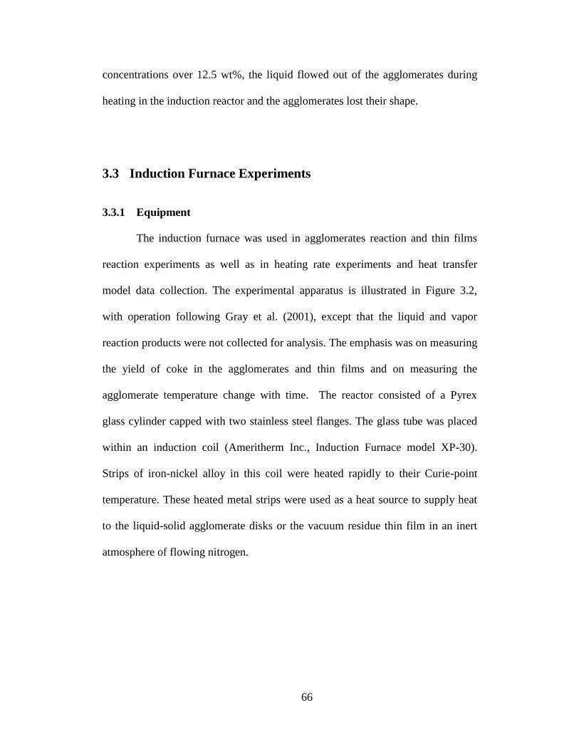
66
concentrations over 12.5 wt%, the liquid flowed out of the agglomerates during
heating in the induction reactor and the agglomerates lost their shape.
3.3 Induction Furnace Experiments
3.3.1 Equipment
The induction furnace was used in agglomerates reaction and thin films
reaction experiments as well as in heating rate experiments and heat transfer
model data collection. The experimental apparatus is illustrated in Figure 3.2,
with operation following Gray et al. (2001), except that the liquid and vapor
reaction products were not collected for analysis. The emphasis was on measuring
the yield of coke in the agglomerates and thin films and on measuring the
agglomerate temperature change with time. The reactor consisted of a Pyrex
glass cylinder capped with two stainless steel flanges. The glass tube was placed
within an induction coil (Ameritherm Inc., Induction Furnace model XP-30).
Strips of iron-nickel alloy in this coil were heated rapidly to their Curie-point
temperature. These heated metal strips were used as a heat source to supply heat
to the liquid-solid agglomerate disks or the vacuum residue thin film in an inert
atmosphere of flowing nitrogen.

67
Figure 3.2: Schematic diagram of the induction furnace reactor

68
3.3.2 Experimental Procedure
3.3.2.1 Ultimate Coke Yield in Agglomerates
For induction furnace experiments, disk shaped AVR-coke agglomerates
with 15mm diameter were prepared with thicknesses of 2 mm, 3 mm and 4 mm
and with AVR concentration of 8%, 10% and 12.5% by weight. These dimensions
ensured that the geometry for the evolution of products was approximated by a
one-dimensional length scale.
The moisture-free weight of the agglomerates was determined by heating
them in a vacuum oven at 70 oC for about one hour then weighing them in a
moisture analyzer (Mettler Toledo HB43). Special care was required in storing,
handling, and weighing the samples because the solid coke particles were
hygroscopic. Uncontrolled moisture uptake was significant in comparison to the
yield of coke, and gave biased coke yields that were too low. Agglomerates were
then placed between two perforated Curie point strips (Figure 3.3). Perforation on
the Curie-point alloys were 0.61 mm holes on 1.5 mm triangular pitch. Both lower
and upper strips were sprayed with a thin layer of bitumen to ensure good contact
with the agglomerate in both sides. The sprayed strips were then warmed up and
the agglomerate placed between them and the assembly was clamped and cooled
to glue the agglomerate to the strips and to ensure good contact with both strips.
The assembly of the agglomerate and the strips was placed inside the
induction furnace (Figure 3.2), the reactor was sealed and purged with nitrogen
for 15 minutes then the strips were heated to their Curie-point temperature by the

69
application of the induction field. Both the upper and lower strips heated the
agglomerate by conduction and allowed vapor products to escape through the
holes. The vapors were removed from the reacting agglomerates by flowing
nitrogen gas at a flow rate of 12 sL/min. The agglomerates were reacted for
enough time, depending on their AVR content and thickness, to ensure total
conversion of the AVR in the agglomerates to toluene-insoluble coke and volatile
products. The 2mm and 3mm agglomerates with AVR concentration below 12.5%
were reacted for 10 minutes. The 4 mm agglomerates and 2 mm and 3 mm with
12.5% AVR were reacted for 15 minutes. Two different compositions of Curie-
point alloy were used to provide two different reaction temperatures; 503oC and
530oC. After coking, several agglomerates were tested for any unreacted bitumen
by dissolving them in toluene, but no soluble bitumen components were detected.
The weight of coke after the reaction was determined and the amount of
new coke formed was calculated by difference. Coke mass was determined by
using a moisture analyzer (Mettler Toledo HB43) that heats the sample up to 110
oC and determine the dry weight of coke. Coke yield was calculated as the ratio of
the new coke formed over the initial amount of bitumen in the agglomerate.
AVRinitialofMass
cokeinitialofmasscokefinalofMassYieldCoke
(3.1)

70
Figure 3.3: AVR-solids agglomerate between two perforated Curie-point
strips

71
3.3.2.2 Ultimate Coke Yield in Thin Films
Thin films of AVR were reacted to determine the ultimate coke yield and
to compare it to the ultimate coke yield in agglomerates. For thin film
experiments, the vacuum residue material was coated onto strips of Ni/Fe alloy
(25 cm x 2 cm x 0.04 cm) with Curie-point temperatures in the range of 503 °C,
following Soundararajan (2001). Up to six strips were held in ceramic holders to
form an annulus within a Pyrex glass cylinder capped with stainless steel flanges.
Both the alloy strips and the glass tube were held within the induction coil
(Ameritherm Inc., induction furnace model XP-30). Nitrogen sweep gas was
introduced at one end of the glass tube through a sintered metal diffuser and
exited the opposite end through a conical section. The gas flow rates used for the
experiments were 12 sL/min.
Thin films of feed material are created by dissolving the feed in methylene
chloride, then spraying the solution onto the strips. The strips were dried
overnight and reweighed to determine the amount of vacuum residue or
asphaltene deposited. Mean film thickness was in the range 20-80 m in all
experiments, calculated as volume of residue divided by the area coated.
The entire system sealed and purged with nitrogen for 15 min. The
induction heater was then turned on and the strips brought to reaction temperature
for 4 min to allow for complete coking to occur. At the end of this time, the alloy
strips were cooled and the amount of coke on the strips after the reaction was
determined by weight and the coke yield was calculated.
72
By adjusting the settings on the induction heater, the times for heating the
strips could be adjusted between 3 s and 45 s. These heating times correspond to
heating rates in the range of 14.8 K/s to 148 K/s, a difference of a factor of ten.
Consequently, the equipment was able to give heating rates that varied over an
order of magnitude.
3.3.3 Agglomerates Temperature Profile Measurement
For measuring the temperature profile inside the agglomerates and the
temperatures of the Curie-point strips, three type-K, 24 AWG gauge
thermocouples were used. Two thermocouples were spot welded to the inner side
of both Curie-point strips, i.e. between the Curie-point strips and the outer
surfaces of the agglomerate. The third thermocouple was inserted between two
agglomerates of equal thickness to measure the centre-line temperature of the
agglomerate. The Curie-point strips and agglomerate assembly with the
thermocouples was then reacted in the induction furnace following the same
procedure in section 3.3.2.1 and temperature data was recorded using a HP
BenchLink Data Recorder. A schematic of the assembly is shown in Figure 3.4.

73
Figure 3.4: Schematic diagram of the assembly of agglomerates, strips and
thermocouples. Thermocouples were used for temperature profile
experiments
AVR-coke
agglomerate
Bottom Curie point strip
Upper Curie
point strip
Top
Thermocouple
Middle
Thermocouple
Bottom
Thermocouple

74
3.4 Fluidized Bed Reactor
3.4.1 Equipment
The fluidized bed reactor was used in determining the coke yield in AVR-
solids agglomerates and in testing the agglomerate behavior under fluidized
conditions. Figure 3.5 shows a schematic diagram of the reactor. The fluidized
reactor section consists of a 102 mm (4-inch) diameter heated section connected
to an upper free board 10-inch diameter column and a 32 mm (1.25-inch)
diameter sidearm for agglomerate injection. The side arm contains a gate valve at
the bottom to hold the agglomerate before the injection. A flow of nitrogen was
used for aeration to avoid raise in arm temperature and to prevent agglomerates
from sticking to the side arm wall or to each other. The bottom of the fluidized
reactor consists of a 102 mm (4-inch) tall conical section that contains three
stainless steel gas distributors. At the top of the fluidized reactor, in the 254 mm
(10-inch) free board section, two internal cyclones are connected in series to
remove the fine fluidization particles from the exit gas stream.
Five band heaters (114.3 mm ID 50.8 mm wide for each heater) totaling
3350 W are employed to supply the heat to the fluidized bed. The fluidized
section of the reactor is equipped with six thermocouples to measure the fluidized
bed, free board and reactor body temperatures and with pressure transducers to
monitor the reactor pressure.
The fluidized reactor is connected to a bottom quench section through a
102 mm (4-inch) diameter ball valve. The 204 mm (8-inch) diameter bottom

75
section contains a fluidized bed that can be used for rapid quenching or cooling of
hot solids from the reactor bed, if needed. The gas distributor for the bottom
section consists of 4 radial sparger tubes. A 204 mm (8-inch) diameter knife gate
valve is used to close the bottom section of the reactor. A blind flange is used at
the bottom of the 204 mm (8-inch) gate valve to give a good seal for the bottom
quenching section of the reactor. Three thermocouples and a pressure transducer
are used to monitor the bottom section temperature and pressure, respectively. A
cooling water jacket is used at the top of the bottom section below the ball valve
to prevent the heat flow by conduction from the fluidization column to the bottom
section.
Fluidization gas to the reactor was heated by a sand bath heater and an
electric heater in series. Fluidization gas temperature after the electric heater was
monitored and controlled through the power output of the electric heater.

76
Figure 3.5: Schematic diagram of the fluidized bed reactor assembly

77
3.4.2 Experimental Procedure
3.4.2.1 Ultimate Coke Yield in Fluidized Bed Reactor
To determine the ultimate coke yield in reaction of AVR-solids
agglomerates, cylindrical agglomerates of 1:1 aspect ratio were made out of AVR
and aluminum oxide and tested in the fluidized bed reactor (Figure 3.5). AVR-
alumina agglomerates were made with sizes of 5 mm, 10 mm and 15 mm and
with AVR concentrations of 8%, 10% and 12.5%. 120µ Alumina particles,
classified ad Type B according to Geldart Classification, was used in making
agglomerates and as fluidization solids in order to be able to determine the
amount of coke formed after the reaction by burning the bed charge and
determining the amount of CO2 by absorption in alkaline solution.
3.5 kg of alumina was used as fluidization solids in the reactor section.
The ball valve between the reactor section and the bottom section was first closed,
and the alumina was loaded through the agglomerate injection arm. After loading
the alumina particles to the reactor, the 50 mm (2-inch) knife gate valve at the
bottom of the agglomerate injection arm was closed. The desired amount of
agglomerates for the experiments was prepared: 3 agglomerates of the 15 mm, 5
agglomerates of the 10 mm or 20 agglomerates of the 5 mm. The agglomerates
were weighted and the mass was recorded, then the agglomerates were mixed
with suitable amount of alumina, from 50g to 120g depending on the amount of
agglomerates, to prevent the agglomerates from sticking to each other or to the
walls of the loading arm before injection into to the reactor. The agglomerates and
the alumina mix was then loaded into the agglomerates injection arm and the arm

78
was sealed and closed. Aeration nitrogen kept flowing to the agglomerate
injection arm to keep the agglomerate at the room temperature and prevent them
from melting or sticking together. All the reactor connections were checked for
leakage and the whole reactor was purged with nitrogen for 1h.
After purging, the fluidization nitrogen was set at 10.44 sL/min during the
heating up period. The preheating system (the sand bath and the electric heater)
and the reactor bed band heater were switched on and the desired temperature set
point was given to the temperature controllers. When the desired temperature was
reached in the reactor, the nitrogen flow was switched to the high flow position at
52.4 sL/min (equivalent to 40 U/Umf and bubbling regime fluidization) and the
reactor was left to fluidize for 10 more minutes for the temperature to stabilize.
Before agglomerate injection, the pressure in the agglomerate injection
arm was increased to 1 psi higher than the pressure in the reactor. To inject the
agglomerate to the reactor bed, the 50 mm (2-inch) knife gate valve was opened,
allowing the agglomerates and the mixing alumina to drop into the reactor. The
agglomerates were then left to react in the fluidized bed for 30 minutes to ensure
complete conversion of the feed AVR to coke.
To calculate the amount of coke formed during the reaction, the
fluidization gas was switched to oxygen with flow of 10.4 sL/min to burn the
coke in the bed for about from 6 to 7 hours. The carbon dioxide from the
combustion of coke was absorbed in alkali solution in a system of bubbling
absorber bottles and used to determine the amount of coke based on the change in

79
the solution electrical conductivity. Four 500-mL absorption bottles, supplied by
Fisher Scientific, were used in two parallel arrangements. The gas entered the
bottles through fritted glass cylinders. Barium hydroxide (Ba(OH)2) was used as
an absorbent for the combustion products gases, after the method used by
Raymond and Winegarden (1927) to determine the CO2 in fermenting mixtures.
After each run, the absorption bottles were washed with hydrochloric acid (Fisher
Scientific) to remove the deposited barium carbonate and to clean the clogged
pores of the sparger tube. A calibration curve was made between the amount of
coke burned in the bed and the corresponding change in the electrical conductivity
of the Ba(OH)2 solution by burning a known amount of coke and record the
change of the electrical conductivity (Appendix A).
The amount of coke then recorded and the coke yield was calculated
relative to the initial amount of AVR in the agglomerates.
AVR ofamount Initial
reactor in the formedcokeofAmountYieldCoke (3.2)

80
3.4.2.2 Fragmentation of Agglomerates in Fluidized Bed Reactor
The survival and fragmentation of the AVR-alumina agglomerates were
studied to link and compare the results of this study to the study of AVR-coke
agglomerates done by Weber (2009).
Before loading the fluidization alumina to the reactor bed, 8kg of alumina
was loaded into the bottom quench section of the reactor to help cool the reactor
charge once dropped in the bottom section after reaction, and also to prevent
breaking of agglomerates when dropped to the bottom section. The bottom section
alumina was loaded through the agglomerates injection arm while the ball valve
between the reactor section and the bottom section was open. Once the alumina
was loaded to the bottom section, the ball valve was closed and the reactor
loading and purging procedures were performed similarly as mentioned in the
previous section. After reaction of the agglomerates for 30 minutes, the ball valve
was opened allowing the agglomerates to drop to the bottom section, where
fluidization and cooling nitrogen gas was introduced through the gas distributor at
the bottom of the bed. When the temperature of the agglomerates dropped to
about 60-70oC, the bottom knife gate valve was opened and the agglomerates
along with the fluidization alumina was collected. To separate the agglomerates
from the fluidization alumina, the collected solids from the bed were sieved using
500 µm screen (38 mesh number). The mass of the agglomerates and fragments
larger than 500 µm was then recorded and presented as a fraction of the initial
mass of agglomerates before reaction.

81
3.5 Thermogravimetric Analysis of Agglomerate and Thin Film
Coke
Samples from both thin films and agglomerate coke were prepared using
the standard procedures used in determining the ultimate coke yield in thin films
and agglomerates. The coke samples were then tested in a TGA to determine the
amount trapped volatile materials in both cases.
TGA was performed in Thermo Cahn Thermax 300 machine. After
loading the sample to the TGA, the TGA was then purged with 80 mL/min flow
of argon at the room temperature. The temperature was then increased to 500oC at
a rate of 20oC/min. when the temperature reached 500
oC, it was kept at this
temperature for about 1 hour. After the constant temperature period was complete,
the gas flow was switched to air for one more hour to burn the sample and
determine the amount of coke solids in the initial sample.

82
4 RESULTS
4.1 Coke Yield in Agglomerates in Induction Furnace1
Three variables were studied to investigate their effect on the ultimate
coke yield in AVR-coke agglomerates: (1) Concentrations of AVR of 8%, 10%
and 12.5 wt%, corresponding to 20%, 26% and 30% of the pore volume,
respectively, (2) Agglomerate thicknesses of 2 mm, 3 mm, and 4 mm, and (3)
reaction temperatures of 503 oC and 530
oC. For every tested variable, enough
replicate experiments were conducted to determine the mean yield of coke and the
standard error. In some cases, data sets were tested for outliers or tested for
statistical significance. Thin films of 20µm thickness AVR were made on the
Curie-point alloys and were tested at 503oC to compare the coke yield from the
thin films to coke yield from liquid-solid agglomerates.
4.1.1 Coke Yield from Agglomerate versus Thin Films
Figure 4.1 shows the average coke yield from 20 µm thin films and from AVR-
coke agglomerates. The average coke yield at 503oC in the case of the
agglomerates was found to be 23.3±1.7%. For the same AVR feed, the coke yield
of reaction of thin films of 20 μm was 11.7±0.3% at the same temperature. Higher
coke yield in the agglomerates supported the idea that mass transfer played a role
in increasing the coke yield. The liquid films within the agglomerates would be
thicker than the case of the sprayed liquid film, due to liquid bridges between
particles and incomplete wettability of solids, which means the cracking products
1 Portions of Section 4.1 were published in Ali et al. Can J Chem Eng, 2010, v 88, issue 1, 48-54

83
will have longer diffusion paths to exit the liquid phase and a better chance to be
trapped in the liquid and undergo the undesired coke forming side reactions.

84
Figure 4.1: Average coke yield in 20 µm AVR films and AVR-coke
agglomerates at 503oC in induction furnace. The error bars represents the
standard errors from replicate experiments
0
5
10
15
20
25
30
Cok
e Y
ield
(%
)
20 Micrometer thin film
Agglomerate disks - Induction furnace
85
4.1.2 Miscroscopy of Vacuum Residue and Coke in Agglomerates
In order to visualize the environment of the vacuum residue reacting in
coke agglomerates, micrographs were obtained of agglomerated material. Figure
4.2 shows a scanning electron micrograph for the AVR-coke agglomerate. The
micrograph clearly show the uneven distribution of the liquid AVR over the coke
particles, and the liquid bridges formed between the solid particles with lengths
up to 120 µm (Figure 4.2). Polarized Light Microscopy (PLM) of the
agglomerates after reaction showed that coke was formed in the thick layers and
in the liquid bridges between particles (Figure 4.3). Similar coke formation in
liquid bridges and particle fusion was noted in the SEM images of surviving
agglomerates (peas and beans) in the industrial fluid coker (Figure 4.4). From
these images, we conclude that bridges of liquid between coke particles react to
form bridges of coke, and that the distances for transport of products in this bridge
geometry are long in comparison to the thin films coated on flat surfaces. It is
noted in the micrographs that there is a difference in color of the coke particles
and the coke formed during the reaction. The difference in the coke appearance
can be explained by the difference in the temperature and reaction time history
that the different types of cokes have been subjected to. The particle coke
(obtained from Syncrude fluid coker) passed through multiple cycles between the
fluid coker and the burner and was subjected to temperatures as high as 600 oC,
while the coke formed in layers and liquid bridges during the reaction was
subjected only to the reaction temperature (from 503 to 530 oC) and for a single
reaction path.

86
Figure 4.2: Electron microscopy images of AVR-coke agglomerates with
12.5% AVR by weight showing the liquid distribution over the solid particles
and the formation of liquid bridges between the particles.
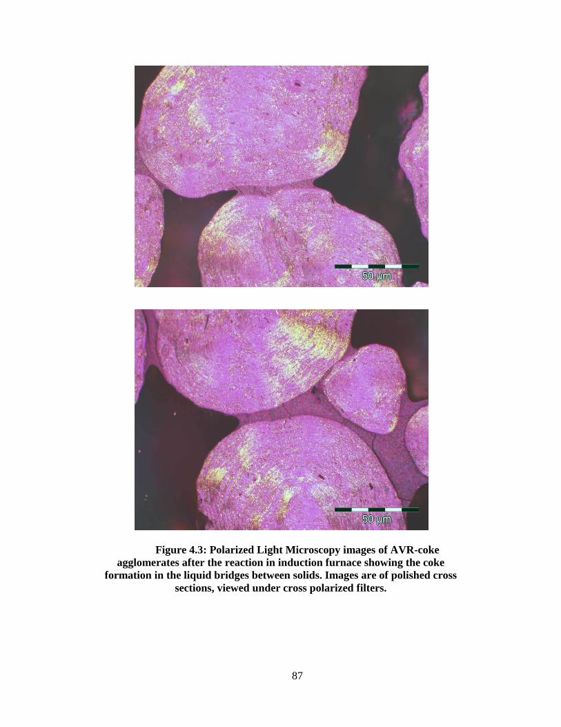
87
Figure 4.3: Polarized Light Microscopy images of AVR-coke
agglomerates after the reaction in induction furnace showing the coke
formation in the liquid bridges between solids. Images are of polished cross
sections, viewed under cross polarized filters.

88
Figure 4.4: Scanning Electron Microscopy images of the surviving
agglomerates (peas and beans) in the fluid cocker showing the formation of
coke in the liquid bridges between coke particles. Images are of polished
cross sections of agglomerated material, taken in the back-scattered mode

89
4.1.3 Agglomerate Thickness
The data of Figure 4.5 show the coke yield in the agglomerates as a
function of the agglomerate thickness for the three different liquid concentrations
at 503 oC. For each of the AVR concentrations, no significant difference in coke
yield was observed. The regression parameters were estimated using the LINEST
function in Microsoft Excel and the Null hypothesis H0: slope=zero was tested by
double-sided t-test with 95% significance and the values of the P-value are
presented in table 4.1 (sample calculations are shown in Appendix B). This result
suggests that reducing the size of agglomerate in a fluidized bed reactor down to 2
mm thickness still does not reduce the effect of mass transfer limitation in the
liquid within the agglomerate. These results also show that any effect due to
varying the heating rate at the center of the agglomerate, due to change in
thickness, was not significant on the ultimate coke yield at long reaction time.
The thicker agglomerates did react more slowly, due to the reduced rate of heating
within the material, but the ultimate yield of coke was insensitive to this change.
Table 4.1: Significance testing P-values for the effect of thickness on coke
yield data
Data Set P-Value Remarks
8% AVR 0.2039 >0.05, no significance
10% AVR 0.9540 >0.05, no significance
12.5% AVR 0.1202 >0.05, no significance

90
Figure 4.5: Effect of agglomerate thickness on ultimate coke yield in
agglomerates of coke and Athabasca Vacuum Residue at 503 oC. The
concentration of AVR in the agglomerates ranged from 8 to 12.5 wt%. Error
bars represent standard error from replicate experiment
0
5
10
15
20
25
30
35
2 3 4
Co
ke
Yie
ld (
%)
Agglomerate Thickness (mm)
8%
10%
12.50%

91
4.1.4 AVR Concentration (Liquid Saturation)
The effect of changing the AVR concentration on the ultimate coke yield
for 3 mm agglomerates is showed in Figure 4.6. Every data point represents a
single batch of liquid-solid mixture. The error bars in the x-axis show the standard
error in determining the actual AVR concentration in the prepared agglomerates,
while the error bars in the y-axis show the standard error due to the variation of
the coke yield. At a given concentration of AVR, the batch-to-batch variation in
both the actual AVR concentration and the corresponding coke yield can be
clearly observed. This batch-to-batch variation was largest at 8 wt% of AVR and
diminished as the AVR concentration was increased.
The coke yield in the case of 8 wt% bitumen agglomerates ranged from 20
% to 32%. In the case of 12.5wt% bitumen concentration, the coke yield ranged
from 20% to 22%. This variability was one of the reasons that AVR
concentrations below 8% could not be studied by this method. The slope of the
data in Figure 4.6 did not indicate the presence of a significant correlation
between the coke yield and AVR concentration in the studied range. The P-value
of the hypothesis testing was 0.0764>0.05, which mean the Null hypothesis that
the slope equals to zero cannot be rejected. This range of AVR concentration
(from 8 to 12.5 wt% AVR by weight, corresponding to 20% to 30% liquid
saturation), was below the saturation concentration of the solid-liquid matrix.
Consequently, the distribution of the liquid on the solid particles would be similar,
meaning no significant changes in the liquid layer thickness within the solid
particles and the diffusion paths due to changes in total liquid concentration. We

92
would expect more liquid to give more bridges between particles, rather than
changing the dimensions of the bridges themselves. Consequently, the mass
transfer limitation within the liquid phase in the agglomerates would be
insensitive to the initial concentration of liquid. Once the vapors exited the liquid
phase, the low liquid saturation would enable easy diffusion and net flow through
the pore space to exit the agglomerates.

93
Figure 4.6: Effect of concentration of Athabasca Vacuum Residue on the
yield of coke yield from 3 mm agglomerates at 503 oC. Error bars in x-axis
represent the standard error in determining the actual AVR concentration in
agglomerates, and in y-axis represent the standard error from replicate
experiments
0
5
10
15
20
25
30
35
40
6 7 8 9 10 11 12 13 14
Cok
e Y
ield
(%
)
Bitumen Concentration (%)

94
4.1.5 Reaction Temperature
Two different Curie-point alloys with different compositions were used in
the induction furnace to provide two different reaction temperatures for
agglomerates. Figure 4.7 shows the effect of bitumen concentration on the coke
yield for two different reaction temperatures, 503 and 530 oC, for 3 mm
agglomerates. The figure shows that changing the temperature did not have an
effect on the coke yield over the tested range of liquid concentration. Similar
insensitivity of the ultimate coke yield to temperature was observed by Gray et al.
(2004) in coking of thin films.
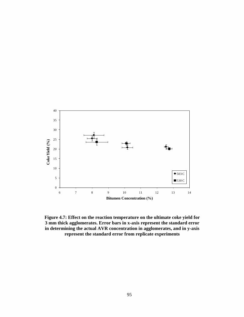
95
Figure 4.7: Effect on the reaction temperature on the ultimate coke yield for
3 mm thick agglomerates. Error bars in x-axis represent the standard error
in determining the actual AVR concentration in agglomerates, and in y-axis
represent the standard error from replicate experiments
0
5
10
15
20
25
30
35
40
6 7 8 9 10 11 12 13 14
Co
ke
Yie
ld (
%)
Bitumen Concentration (%)
503 C
530 C

96
4.1.6 Coke formation from AVR-alumina agglomerates
Before performing the fluidized bed experiments on AVR-alumina
agglomerates, the AVR-alumina agglomerates were tested in the induction
furnace under the same conditions as the AVR-coke agglomerates. The coke yield
from the two different kinds of solids were compared to check if using different
solids in agglomerates would have any effect on the ultimate coke yield.
The 3mm agglomerates were reacted at 503 oC in the induction furnace for
enough time to react all the AVR. Replicate experiments were done to calculate
the average coke yield and the standard error. The significance was tested using
Null Hypothesis H0: slope=zero and double sided t-test with 95% confidence. The
results are shown in Figure 4.8. No significant trend in the coke yield was
observed in the case of AVR-alumina agglomerates. In the cases of 10 wt% and
12.5 wt% bitumen concentrations, coke yield was almost the same in both coke
and alumina agglomerates. A slight different in the coke yield was noticed in the
case of 8 wt% bitumen concentration; however, the data from experiments with 8
wt% bitumen had the highest variation between batches in the case of AVR-coke
agglomerates, and the lowest repeatability in experiments. Consequently, the
difference was not significant between agglomerate made from coke and from
alumina.
Figure 4.9 shows SEM micrographs of the AVR-alumina agglomerates,
which show similar distribution of the liquid to the case of AVR-coke
agglomerates (Figure 4.2), taking into account the different shapes of both solids.
Uneven liquid distribution and liquid bridges also formed between the alumina

97
particles, leading to longer diffusion paths of the reaction products from the liquid
phase to the vapor phase within the pores of the agglomerates. The PLM images
of reacted AVR-alumina agglomerates showed coke formation in the liquid
bridges and thick layers (Figure 4.10), similar to the coke formation in the AVR-
coke agglomerates.

98
Figure 4.8: Comparison between coke yield in induction furnace in the cases
of AVR-coke and AVR-alumina agglomerates at 503 oC and for 3 mm
agglomerates
0
5
10
15
20
25
30
35
7 8 9 10 11 12 13
Co
ke
Yie
ld (
%)
AVR Concentration (%)
AVR-Alumina
AVR-Coke

99
Figure 4.9: Electron microscopy images of AVR-alumina agglomerates with
12.5% AVR by weight showing the liquid distribution over the solid particles
and the formation of liquid bridges between the particles
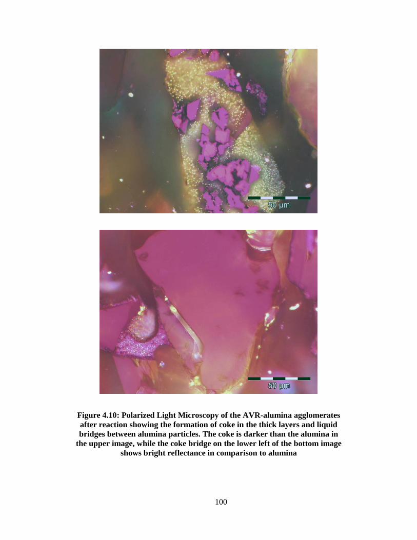
100
Figure 4.10: Polarized Light Microscopy of the AVR-alumina agglomerates
after reaction showing the formation of coke in the thick layers and liquid
bridges between alumina particles. The coke is darker than the alumina in
the upper image, while the coke bridge on the lower left of the bottom image
shows bright reflectance in comparison to alumina

101
4.2 Coke Yield in Agglomerates in Fluidized Bed
Cylindrical agglomerates of AVR and alumina were tested in the fluidized
bed reactor to determine the effects of AVR concentration and agglomerate size
on the ultimate coke yield. The AVR concentration tested were 8%, 10% and
12.5% by weight, equivalent to 20%, 26% and 30% of the pore volume,
respectively. The agglomerate sizes were 5mm, 10mm and 15mm with 1:1 aspect
ratio. The reaction temperature was 500oC and the fluidization velocity was 0.3
m/sec, which gives U/Umf of 40.
Average coke yield from cylindrical agglomerates was 26.4±3%. Coke
yield from AVR-alumina agglomerate disks in induction furnace experiments was
22.0±3.4%. The values of coke yield in AVR-alumina agglomerates from both
the induction furnace and the fluidized bed were significantly higher than the case
of 20 µm film (11.7±0.3%). Figure 4.11 shows a comparison of coke yield of the
two agglomerates types and thin films.
4.2.1 Effect of AVR concentration (Liquid Saturation)
Figure 4.12 shows the result of the coke yield in the agglomerates for
AVR concentrations ranging from 8 wt% to 12.5 wt%. The coke yield in 5mm
and 10mm agglomerates did not show any trend with changing AVR
concentration. Significance testing of the slopes of the regression lines for coke
yield as a function of concentration gave p-values of 0.4627 and 0.0889 for 5mm
and 10mm, respectively. Although the 15mm agglomerates appeared to show a
drop in the coke yield at 12.5 wt%, testing the slope of the regression line gave a
P-value of 0.0737; therefore, the null hypothesis of zero slope could not be
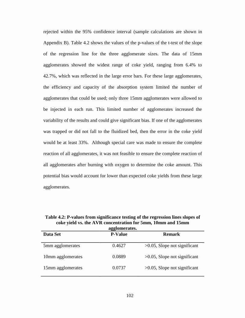
102
rejected within the 95% confidence interval (sample calculations are shown in
Appendix B). Table 4.2 shows the values of the p-values of the t-test of the slope
of the regression line for the three agglomerate sizes. The data of 15mm
agglomerates showed the widest range of coke yield, ranging from 6.4% to
42.7%, which was reflected in the large error bars. For these large agglomerates,
the efficiency and capacity of the absorption system limited the number of
agglomerates that could be used; only three 15mm agglomerates were allowed to
be injected in each run. This limited number of agglomerates increased the
variability of the results and could give significant bias. If one of the agglomerates
was trapped or did not fall to the fluidized bed, then the error in the coke yield
would be at least 33%. Although special care was made to ensure the complete
reaction of all agglomerates, it was not feasible to ensure the complete reaction of
all agglomerates after burning with oxygen to determine the coke amount. This
potential bias would account for lower than expected coke yields from these large
agglomerates.
Table 4.2: P-values from significance testing of the regression lines slopes of
coke yield vs. the AVR concentration for 5mm, 10mm and 15mm
agglomerates.
Data Set P-Value Remark
5mm agglomerates 0.4627 >0.05, Slope not significant
10mm agglomerates 0.0889 >0.05, Slope not significant
15mm agglomerates 0.0737 >0.05, Slope not significant

103
Figure 4.11: Average coke yield in 20 µm AVR films, AVR-alumina
agglomerates disks and AVR-alumina cylinders at 500oC. The error bars
represents the standard errors from replicate experiments
0
5
10
15
20
25
30
Co
ke
Yie
ld (
%)
20 Micrometer thin film
Agglomerate disks - Induction
furnace
Agglomerate Cylinders -
Fluidized bed

104
Figure 4.12: Effect of concentration of Athabasca Vacuum Residue on the
yield of coke from 5 mm, 10 mm and 15 mm agglomerates of AVR and
alumina at 500 oC in the fluidized bed reactor. Error bars in x-axis represent
the standard error in determining the actual AVR concentration in
agglomerates, and in y-axis represent the standard error from replicate
experiments
0
5
10
15
20
25
30
35
7 8 9 10 11 12 13 14
Co
ke
Yie
ld (
%)
Bitumen Concentration (%)
5mm
10mm
15mm

105
4.2.2 Effect of Agglomerate Size
The effect of the agglomerate size on coke yield is shown in figure 4.13.
The data shows that there was no significant change in the average coke yield
with changing the agglomerate sizes at all AVR concentrations (ANOVA test
worksheet is shown in Appendix B). Similar to the observation in the previous
section, the 15 mm-12.5wt% agglomerates showed lower values than the rest of
the data. The data for the 15 mm agglomerates also showed the widest error bars
due to the high experimental error associated with injecting only three
agglomerates to the reactor. The analysis of variance testing for the data group
showed, with 95% confidence, that there was no significant difference between
the mean values within the whole data range or within the 15 mm agglomerate
data. The following table shows the results of the analysis of variance testing.
Table 4.3: Analysis of variance results for testing the means of the results for
15mm alumina agglomerates and whole data range for significance
Data Set P-Value Remarks
15 mm agglomerates 0.6040 >0.05, same mean values
Whole data range 0.9269 >0.05, same mean values

106
Figure 4.13: Effect of the size of alumina agglomerates on the yield of coke at
500 oC for 8%, 10% and 12.5% AVR concentrations in the fluidized bed
reactor. Error bars in y-axis represent the standard error from replicate
experiments
0
5
10
15
20
25
30
35
40
5 10 15
Cok
e Y
ield
(%
)
Agglomerate size (mm)
8%
10%
12.50%

107
4.3 Agglomerate Survival in Fluidized Bed
AVR-alumina cylindrical agglomerates, similar to the agglomerates used
in the coke yield determination in fluidized bed, were tested for survival under the
reaction conditions. Agglomerates with different sizes and different liquid
saturation were reacted in the fluidized for enough time for complete conversion
of heavy oil. The surviving agglomerates were then separated from the
fluidization silica particles to determine the survived agglomerates fractions. A
1000 µm (mesh No. 18) screen was used to separate the agglomerates and their
fractions from the 120µm fluidized silica particles. The mass of the surviving
agglomerates and fractions larger than 1000µm was compared to the initial
agglomerates’ mass and the survival was determined as a fraction from the initial
mass. Three agglomerates sizes were tested: 5mm, 10mm and 15mm, over the
range of bitumen concentration from 8% to 12.5% by weight at 500oC and U/Umf
of 40. The results showed that at these conditions some disintegration and
fractionation have occurred, but the average mass of the agglomerate fractions
above 1000µm was in the range of 0.91 to 0.97 compared to the initial
agglomerates mass (Figure 4.14). Visual inspection showed that most of the
agglomerates stayed intact and survived the reacting conditions with minimum
fracturing and some notable attrition to give near spherical agglomerates (Figure
4.15).

108
Figure 4.14: The mass ratio of survived agglomerates to initial agglomerate
mass of reacting AVR-silica agglomerates at 500oC and 40 U/Umf. The AVR
concentration ranged from 8% to 12.5% at agglomerate sizes of 5mm, 10mm
and 15mm cylinders
0
0.2
0.4
0.6
0.8
1
1.2
1.4
1.6
5 10 15
Su
rvie
d F
ract
ion
Agglomerate size (mm)
8%
10%
12.50%

109
Figure 4.15: Photos of 15mm and 10% AVR concentration agglomerates
before and after reaction
Before
After

110
4.4 TGA of Agglomerates and Thin Film Coke Samples
Agglomerate coke and thin-film coke were tested by the TGA to
determine and compare the amount of trapped crackable materials in each type of
coke material. Agglomerate coke was prepared by reaction of AVR-alumina
agglomerates of 3 mm thickness and 10% initial AVR concentration. The thin-
film coke was prepared by reaction of 20 µm and 60 µm initial thickness of AVR
on Curie-point strips. Each sample of the coke was loaded to the TGA apparatus
(Thermo Cahn Thermax 300) and the apparatus was purged with argon at room
temperature then the temperature was raised at 20oC/min until it reached 500
oC.
The sample was then heated at 500oC for 1 hour. After the reaction time was
ended, the gas flow was then switched to oxygen to burn the carbonaceous
materials for an additional 1 hour to determine the amount of mineral solids in the
initial sample weight. In the agglomerate coke the mineral solids were the
alumina in the initial agglomerate. In the case of coke from thin film experiments,
the mineral solids were metal fragments from scraping the Curie-point strips to
remove the coke from the strip.
Figure 4-16 to 4-18 show the TGA data for the different kinds of coke.
The weight loss due to of devolatilization of coke materials was calculated as the
decrease of the sample weight starting at 450oC till the end of the 500
oC reaction
period. The weight at the end of the run was the weight of the initial mineral
solids. The weight loss in the sample during the reaction period was then
presented as a per cent of the initial sample weight, excluding the weight of
mineral solids (Figure 4.19). The initial rate of devolatilization was calculated as

111
the slope of the weight decrease during the first stage of the reaction period under
an argon atmosphere and was normalized by dividing by the initial amount of
coke in the sample. Calculations of initial mass loss and initial rate of
devolatiliztion are presented in Appendix C
The coke from the 20 µm film of vacuum residue showed the lowest per
cent loss in weight, at 4.3%, while the per cent weight loss in the cases of 60 µm
film coke and agglomerate coke were close to each other at 9.4% and 10.1%,
respectively (Figure 4.19). The 20 µm film coke also gave the lowest initial rate
of devolatilization compared to 60 µm film coke and agglomerate coke. The
initial rate of devolatilization for the 20 µm film coke was 0.004 mg/min/mg
coke, compared to 0.014 mg/min/mg coke for the 60 µm film coke and 0.030
mg/min/mg coke for the agglomerate coke (Figure 4.20).
The low per cent loss in the sample weight and low initial rate of
devolatilization for the 20 µm film coke, in comparison to the two other coke
samples, was consistent with the role of mass transfer limitations in the reacting
film. The decreased tendency to trap volatile products of reaction within the 20
with the role of longer diffusion paths in trapping coke.
The agglomerates coke showed higher initial rate of devolatilization
followed by the 60 µm film coke then the 20 µm film coke. These results show
the higher tendency of trapping to the volatile materials in the thick liquid films
and liquid bridges in the case of agglomerate coke. Lower thicknesses of the

112
reaction liquid films lead to lower diffusion paths and lower tendency of trapping
of volatile materials (Figure 4.20).

113
Figure 4.16: TGA results for the 20 µm film coke showing the decrease of the
sample weight and the temperature data with time
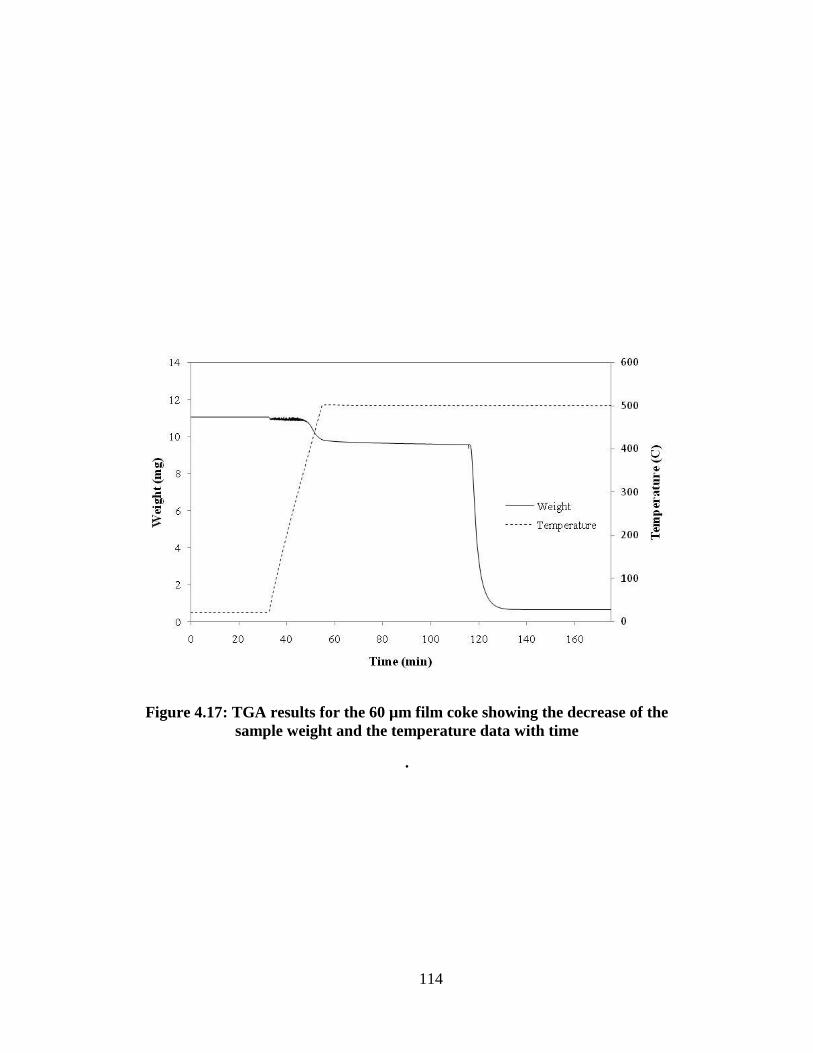
114
Figure 4.17: TGA results for the 60 µm film coke showing the decrease of the
sample weight and the temperature data with time
.

115
Figure 4.18: TGA results for the agglomerate coke showing the decrease of
the sample weight and the temperature data with time

116
Figure 4.19: Per cent weight loss during the reaction period in the TGA for
the three different types of coke
0
2
4
6
8
10
12
20 µm Film 60 µm Film Agglomerate
% W
eig
ht
Lo
ss
Coke Type

117
Figure 4.20: Normalized initial rate of devolatilization in the TGA for the
three different types of coke
0
0.005
0.01
0.015
0.02
0.025
0.03
0.035
20 µm Film 60 µm Film Agglomerate
Init
ial
Ra
te o
f D
evo
lata
liza
tio
n
(mg
/min
/mg
co
ke)
Coke Type

118
4.5 Temperature Profiles and Heat Transfer Model2
Unlike the reactions of thin films on Curie-point strips, the temperature
within a heated agglomerate would increase with time by conduction from the
heated strips to the interior of the agglomerate. The temperature profile within the
reacting agglomerates was measured in the induction furnace by inserting three
thermocouples as described in section 3.3.3 and in Figure 3.5. These agglomerates
were then reacted according to the standard procedure. Figure 4.21 shows the
temperature of the Curie point strips and the corresponding temperature at the
centre of the agglomerate during heating by the induction coil. The heating rate
was calculated as the slope of the linear portion of the time-temperature response.
The heating rate within the agglomerate varied from 80 K/s at the Curie-point
strip to 15 K/s at the center of the agglomerate.
2 This section was published in Ali et al. Can J Chem Eng, 2010, v 88, issue 1, 48-54

119
Figure 4.21: Temperatures of the Curie-point strip and at the centre of the
agglomerate during heating at 503 oC. The total agglomerate thickness was 4
mm, with a thermocouple placed in the centre as illustrated in Figure 3.5
0
100
200
300
400
500
600
0 20 40 60 80 100 120
Tem
per
atu
re (
C)
Time (sec)
T of Curie-point strip
Center T

120
4.5.1 Heat Transfer Model
In order to model the temperature profile, a transient heat transfer model
was used to describe the change of the temperature with the time and location
within the agglomerates. The amount of AVR in the agglomerates was well below
the saturation limit (liquid saturation was in the range of 40 to 50% AVR by
weight).
The following assumptions were used in the proposed model:
The AVR reacted rapidly to give shrinkage in volume and much
higher viscosity, therefore, the AVR-solid mixture was
approximated as a porous solid phase with a single effective
thermal diffusivity (αeff).
The porosity of the porous solid assumed to be constant, due to
low liquid loading of agglomerates
Heats of reaction and vaporization are negligible
The fluid phase was assumed to be nitrogen gas at the reaction
conditions.
The heat flux (T/x ) at the center of the agglomerate equals to
zero
Heat transfer from the heating Curie-point strips to agglomerates is
only by conduction.
The relation between the temperature T at any time (t) and distance from
agglomerate centre line (x) is given as follows:

121
)3.4(02
2
x
T
t
Teff
The following initial and boundary conditions were used:
)6.4(,
)5.4(0,0
)4.4(0, 0
tTtLT
tx
T
TxT
Where T0 is the initial agglomerate temperature before heating, T/x is
the heat flux at the centre of the agglomerate and T(L,t) is the measured
temperature of the Curie-point strip as a function of time.
The effective thermal diffusivity of the agglomerate, eff, was used as the
only adjustable parameter to fit the model to the experimental data. The model
was solved by MATLAB (Appendix D) for a series of experiments, each with a
measured boundary condition (strip temperature). The sum of squared residuals
(SSR) was calculated and minimized to obtain the best value of eff to fit the data.
The MATLAB code for solving the model is presented in appendix B.
7.42
exp predTTSSR
The best fit value of the effective thermal diffusivity was 0.20 x 10⁻⁶
m2/s
with a minimum value of the sum of squared residuals (SSR) of 62660. For the
case of heat transfer in a porous solid, Bejan and Kraus (2003) and Rohsenow et
al. (1998) recommended the following relations to predict the effective thermal
diffusivity of porous media:

122
Where m is the mean thermal diffusivity, km, kfluid and ksolid are the mean,
fluid phase and solid phase thermal conductivities respectively, (Cp)fluid and
(Cp)solid are the heat capacities of the fluid and solid phases respectively, is the
heat capacity ratio, and is the porosity of the porous solid. Using the range of
physical properties of fluid coke materials measured by Michaelian et al. (2002)
and agglomerate porosity of 35% in equations (4.8)-(4.11), the predicted range of
the effective thermal diffusivity for the agglomerates was 0.18 x 10⁻⁶
m2/s to 0.34
x 10-6
m2/s.
Figures 4.22 to 4.24 show the experimental and model data of the
temperature profile within the agglomerates of different thicknesses and initial
AVR concentration. The model showed good agreement with the experimental
data for the different agglomerate sizes and initial AVR concentrations. Figures
4.22 and 4.23 show that increasing the agglomerate thickness affected the rate of
heating of the agglomerate, which was expected, but this change in the heating
rate did not affect the ultimate coke yield as shown previously in the results of the
effect of agglomerates thickness on coke yield. From the experimental results and
11.41
10.41
9.4
8.4
fluidP
solid
solidfluidm
fluidP
m
m
m
eff
C
C
kkk
C
k

123
the model, the heating rates ranged from 80 K/s at the contact with the strips to 15
K/s at the centerline of the agglomerate.

124
Figure 4.22: Experimental and model predicted temperature profile within
an agglomerate of total thickness of 4 mm with thermocouple placed in the
center and bitumen concentration of 10%
0
100
200
300
400
500
600
0 10 20 30 40 50 60 70 80 90 100
Tem
per
atu
re (C
)
Time (sec)
Model
Center T

125
Figure 4.23: Experimental and model predicted temperature profile within
an agglomerate of total thickness of 6 mm with thermocouple placed in the
center and bitumen concentration of 10%
0
100
200
300
400
500
600
0 10 20 30 40 50 60 70 80 90 100 110 120
Tem
per
atu
re (C
)
Time (sec)
Model
Center T

126
Figure 4.24: Experimental and model predicted temperature profile within
an agglomerate of total thickness of 4 mm with thermocouple placed in the
center and bitumen concentration of 12.5%
0
100
200
300
400
500
600
0 10 20 30 40 50 60 70 80 90 100
Tem
per
atu
re (
C)
Time (sec)
Model
Center T

127
4.5.2 Role of Heating Rate
In pyrolysis of solids, such as coal and biomass, the yield of char is
commonly observed to vary with heating rate (Wen and Lee, 1979). In order to
check the role of heating rate in the coking reactions and its effect on the yield of
coke from vacuum residues in agglomerates, coking of different vacuum residue
materials was carried out on Curie point strips at different heating rates. Thin
films of Athabasca vacuum residue (lab-prepared sample), Maya, and Khafji were
reacted at low and high heating rates of 14.8 to 148 K/s. The heating rate was
reduced by detuning the induction coil to give less efficient coupling of the strips
with the induction field.
The data of Table 4.4 and Figure 4.25 show that the yield of coke from
Athabasca vacuum residue #2 was insensitive to the heating rate. Similarly, the
yield of coke form Maya and Khafji vacuum residues were insensitive to heating
rates in this range. The same trends were observed for thinner films of 20 mm
thickness.
The heating rate in reacting agglomerates varied from 80 K/s to 15 K/s,
which lies in the same range that was used to test the heating rate role in thin
films. Given the lack of dependence of the final coke yield on heating rate in film
samples, we conclude that the rate of heating of vacuum residue within the
agglomerates was not a significant factor. Heating rate would have a dramatic
effect on the initial rates of cracking and coking, but the present comparison is on
the final coke yield when the reaction is essentially complete.

128
Table 4.4: Coke yields from 80 µm films of vacuum residues at
503 C
Feed RF Setting % Heating Rate, K/s Coke Yield %
Athabasca VR#2 38.1 14.8 18.20
Athabasca VR#2 -5.0 148 18.80
Maya 38.1 14.8 22.85*
Maya 3.0 80 21.30
Maya -5.0 148 21.55*
Khafji 38.1 14.8 18.00*
Khafji 3.0 80 16.50*
Khafji -5.0 148 17.75*
* indicates mean value of two replicate experiments

129
Figure 4.25: Effect of heating rate on the ultimate coke yield in reacting 20
µm thin films of Maya and Khafji feeds at 503 and 530o C
0
5
10
15
20
0 20 40 60 80 100 120 140 160
Cok
e Y
ield
(%
)
Heating rate (K/s)
Maya 503C
Maya 530C
Khafji 503C
Khafji 530C
Heating rate range for the case of
reacting AVR-coke agglomerates

130
5 DISCUSSION
5.1 Coke yield in agglomerates
Comparing the coke yield in AVR-coke agglomerates to coke yield from
20 µm thin films showed that the agglomerates gave higher coke yield, both from
induction furnace and fluidized bed reactors, relative to the thin films for the same
feed materials and same reaction temperature. At 503oC, the coke yield from
agglomerates from the induction furnace experiments was 23.3±1.7%, while it
was 11.7±0.3% for the thin films (Figure 4.1).
The increase of coke yield in agglomerates supports the role of mass
transfer in controlling the coke yield over this range of values. In agglomerates,
the liquid within the solid-liquid matrix tends to form thicker layers over the solid
particles due to uneven liquid distribution and the liquid bridges between particles
(Figures 4.2 and 4.9). The thicker liquid films in agglomerates provide longer
diffusion paths for the reaction products and higher tendency for trapping the
products within the reacting liquid film and undergoing undesired condensation
and polymerization reactions. The same role of mass transfer was observed in the
work of Gray et al. (2001), where the coke yield was found to increase with
increasing the initial liquid film of reacting heavy oils. The PLM images of cross
sections of reacted AVR-coke and AVR-alumina agglomerates (Figures 4.3 and
4.10) showed that a significant amount of coke was formed in thick liquid layers
and liquid bridges between the solid particles in agglomerates. A similar
observation was noted in the case of coke formation in the agglomerates of the

131
industrial fluid coker (Figure 4.4). These agglomerates provide significant
porosity for the escape of the cracked products once they escape from the liquid
phase. The key distance for mass transfer is not the dimension of the agglomerates
but rather the distance to diffuse out of a liquid film that is confined between
solids particles.
The data for coke yield showed that decreasing the agglomerate size,
down to 2 mm in the case of agglomerate disks in the induction furnace
experiments and down to 5 mm for the agglomerates cylinders in the fluidized
bed reactor experiments, had no significant effect on the coke yield (Figures 4.5
and 4.13). The reduction in the size of the agglomerates did not affect the
thickness of reacting liquid layers on the solid particles and in liquid bridges
between particles over the studied range of liquid saturation.
The concentration or saturation of liquid also did not have any effect on
coke yield. In the studied AVR concentration range, from 8% to 12.5% (relative
to 20% to 30% liquid saturation), the AVR concentration was below the liquid
saturation concentration in the agglomerates. Below the liquid saturation, the
distribution of liquid within the liquid-solid matrix was not significantly different
at different liquid contents, which led to similar diffusion paths within the liquid
phase and similar mass transfer limitations in that range of liquid concentration,
and hence no significant effect of the AVR concentration on the coke yield was
observed for both the induction furnace and fluidized bed agglomerates (Figure
4.6 and 4.12). The mass transfer resistance was only present in the liquid layers
and bridges in the agglomerates. Once the reaction products reached the void
132
space in the agglomerates they diffused easily to the outer surface of the
agglomerates with relatively no resistance to flow within the gas phase. Higher
liquid saturations would be expected to significantly increase the diffusion path
length to a significant fraction of the agglomerate dimension, but such high liquid
saturations were not attempted in this study due to the poor mechanical properties
of the agglomerates. Furthermore, in this regime the formation of vapor bubbles
would have an impact both on transport of products (Gray et al., 2001) and
probably on the stability and structure of the agglomerates.
Changing the reaction temperature from 503oC to 530
oC in the induction
furnace experiments did not have significant effect on the coke yield from
agglomerates (Figure 4.7). Similar insensitivity of ultimate coke yield to reaction
temperature was observed by Gray et al. (2004) in coking thin films. This
observation indicates that although the rate of cracking and devolatilization of the
products depends on temperature, the ultimate coke yield at long reaction times
tends to be insensitive to temperature.
No effect of the type of solids used in making the AVR-solid agglomerates
was noted when using coke and alumina (Figure 4.8) except for a slight difference
in the case of 8% agglomerates. The difference in the 8% coke yield between the
two different solids agglomerates was likely not significant due to the variability
in the 8% agglomerates from batch to batch (see Figure 4.6) within the same solid
used, due to the low AVR concentration and higher errors in actual AVR and
coke yield determination. Changing the solids had no effect on the coke yield due
to the similar distribution of liquid over the solid particles and in liquid bridges

133
and the incomplete wettability in both cases. The data in Figures 4.2 and 4.9 show
that the distribution of liquid over the coke and alumina particles was similar,
forming uneven liquid layers over the particles and liquid bridges between the
solid particles in both cases.
5.2 Coke Yield and Agglomerate Survival Under Fluidized Bed
Conditions
5.2.1 Coke Yield Under Fluidized Bed Conditions
The average coke yield of AVR-alumina agglomerates was significantly
higher than the coke yield from 20 µm thin films, for both agglomerate disks and
agglomerates cylinders (Figure 4.11). The average coke yield in the AVR-alumina
agglomerates cylinders was 24.6±3.0%, while for the AVR-alumina agglomerates
disks was 22.0±3.4 and for the 20 µm thin films was 11.7±3%.
Similar to the case of AVR-coke agglomerates, the increase in coke yield
in alumina agglomerates compared to thin films supports the role of mass transfer
limitation and is due to the formation of thick layers over the solid particles and
thick liquid bridges between the solids (Figure 4.9), which result in longer
diffusion paths, higher mass transfer resistance and higher tendency of trapping of
the reaction products in the reaction liquid films

134
5.2.2 Survival of Agglomerates Under Fluidized Bed Condition
At the reaction conditions in the fluidized bed, 500oC and U/Umf of 40, the
mass of agglomerates and the fraction of agglomerates that survived was in the
range of 0.91 to 0.97 of the initial agglomerate mass, independent of size and
liquid saturation (Figure 4.14). The visual inspection of the agglomerates after
reaction (Figure 4.15) showed that some fragmentation and attrition had occurred,
but the majority of the agglomerates stayed intact and survived during the reaction
time in the fluidized bed. The rapid change in the AVR physical properties,
especially the rapid increase in the liquid viscosity, with the reaction time tended
to hold the liquid solid agglomerate together and suppress the agglomerate
disintegration. The low value of U/Umf was not sufficient to produce enough force
in the fluidized bed to break up the agglomerates or cause significant attrition.
Weber (2009) tested AVR-coke agglomerates for stability in a fluidized
bed of coke particles. The lowest fluidization velocity that was tested was U/Umf =
40. At this condition, the breakup of agglomerates containing 9% AVR by weight
concentration was insignificant. Disintegration of the AVR-coke agglomerates
was only observed at higher fluidization velocities, corresponding to 80 and 120
U/Umf (Weber, 2009). At U/Umf=80, Weber (2009) observed extensive
fragmentation of the AVR-coke agglomerates. Agglomerates with 9 wt%, 13 wt%
and 16.7 wt% AVR showed a maximum in the mass of fragments of up to 2.2
times the initial agglomerate mass at 40 s. The increase in mass was attributed to
adhesion of bed particles to the wet exterior of the agglomerates. Increasing the
reaction time decreased the final relative mass of fragments to the range from 0.5

135
to 1.3 relative to the initial agglomerate mass, depending on initial liquid content.
It should be noted that the experiments of Weber (2009) were done at much lower
fluidization times compared to the fluidization times in this study, which were
from 20 to 30 min. to ensure complete reaction of the AVR in agglomerates.
The lack of fragmentation of the AVR-alumina agglomerates in this study
(Figure 4.14) at U/Umf of 40 was qualitatively consistent with the lack of
fragmentation observed by Weber (2009) for AVR-coke agglomerates at the same
value of U/Umf. The main difference was the lack of increase in mass of
agglomerates in this study, in contrast to Weber (2009), which could be due to the
long reaction times or differences in the wetting of alumina versus coke.
5.3 TGA of Agglomerates and Thin Film Coke Samples
Results from agglomerates and thin films showed that the higher thickness
of liquid layers and liquid bridges in agglomerates resulted in higher coke yields
compared to thin films. Thicker liquid films and liquid bridges in agglomerates
result in longer diffusion paths of the reaction products, which increases the mass
transfer resistance, especially with the rapid change in the AVR physical
properties, specially viscosity. The longer the diffusion path and the mass transfer
resistance, the higher the tendency to trap volatile products in the coke, and the
higher the tendency of the reaction products to undergo undesired condensation
and coke formation reactions. When cracked products are trapped in the coke, we
hypothesize that the resulting material is more reactive under prolonged heating.
Trapping of cracked products could occur by two mechanisms: addition reactions
between the products and the coke phase, and physical trapping due to the rapid

136
increase in viscosity of the liquid with extent of reaction. Both mechanisms would
give weight loss upon sustained heating, because the coke material would undergo
prolonged cracking of side chains and saturated rings, and some physically
trapped material would escape from the coke phase. Coke samples from reacted
AVR-alumina agglomerates and 20 µm and 60 µm reacting films were tested in
the TGA to test the hypothesis of the effect of agglomeration and increasing film
thickness on trapping volatile materials.
In the TGA data for the coke in agglomerates, 20 µm films and 60 µm
films, the coke from the 20 µm film showed the lowest per cent loss in weight,
followed by the 60 µm film coke, then the agglomerate coke (Figure 4.19). The
20 µm film coke also showed the lowest initial rate of devolatilization compared
to the two other types of coke materials (Figure 4.20). The low per cent loss in the
sample weight and the low initial rate of devolatilization for the 20 µm film coke,
compared to the two other coke samples, was consistent with the role of mass
transfer in the diffusion of reaction products from the reacting film. The higher
tendency of products to become trapped within the thicker films and agglomerates
due to longer diffusion paths gave coke materials that were more reactive under
sustained heating at 500oC.
While the 60 µm film coke and agglomerate coke had comparable per cent
loss in weight, the initial rate of devolatilization was higher in the case of
agglomerate coke compared to the 60 µm film coke (Figure 4.20). The higher
initial rate of devolatilization in agglomerate coke, compared to 60 µm film coke,
can be explained by the uneven distribution and the incomplete wettability of the

137
AVR in the liquid-solid matrix in case of the agglomerates and the formation of
thick liquid layers on the solids and liquid bridges between solids (Figures 4.2 and
4.9).
The coke samples were prepared at the same temperature (500oC) with
reaction times of 2 minutes for the 20 µm and 60 µm films and 10 minutes for
agglomerates to ensure complete conversion of the AVR. These initial reaction
times were relatively short compared to the TGA reaction time (1 h at 500oC).
The longer reaction times at the TGA allowed the coke to undergo more extensive
devolatilization reactions at a low rate. All coke samples showed the highest loss
in weight during the early stages of heating, which can be explained by the
removal of condensed materials from the coke. The higher weight loss and initial
rate of devolatilization in agglomerate coke and 60 µm film coke compared to the
coke from the 20 µm film indicated that the longer diffusion paths and the greater
amount of products trapped in the thicker layers produced a more reactive coke.
The thin films ensured more complete evolution of the reaction products from the
reaction liquid, which gave a less reactive coke material in the TGA. This less
reactive coke material, with low amount of cross linked or trapped products, gave
less loss of mass and less initial rate of devolatilization on extended heating at
500oC.

138
5.4 Temperature Profiles and Heat Transfer Model and Role of
Heating Rate
A transient heat transfer model was used to describe the change of the
temperature with the time and location within the reacting AVR-coke
agglomerates. Over the range of AVR concentrations in this study, the AVR
reacted rapidly to give shrinkage in volume and much higher viscosity, therefore,
the AVR-solid mixture was approximated as a porous solid phase with a single
effective thermal diffusivity (αeff).
The relation between the temperature T at any time (t) and distance from
agglomerate centre line (x) was described by a conduction heat transfer model
described in equations 4.3 to 4.6, where the effective thermal diffusivity of the
agglomerate, eff, was used as the only adjustable parameter to fit the model to the
experimental data. The best fit value of the effective thermal diffusivity was 0.20
x 10-6
m2/s. This value of the effective thermal diffusivity for the AVR-solid
agglomerates in the model was within the range of calculated thermal diffusivities
of porous solids estimated using the equations from 4.8 to 4.11 given by Bejan
and Kraus (2003) and Rohsenow et al. (1998) and using the physical properties
data for coke materials given by Michaelian et al. (2002).
The model showed good agreement with the experimental data for the
different agglomerate sizes and initial bitumen concentrations (Figures 4.22 to
4.24). Increasing the agglomerate thickness affected the rate of heating of the
agglomerate in the range from 80 K/s at the contact with the heating strips to 15
139
K/s at the center of the agglomerate. This change in the heating rate did not affect
the ultimate coke yield, as shown in the results of coke yield from the
agglomerates in the induction furnace experiments.
In order to study the role of heating rate in the coking reactions and its
effect on the yield of coke from vacuum residues, coking of different vacuum
residue materials was carried out on Curie point strips at different heating rates of
14.8 to 148 K/s. The results shown in table 4.3 and Figure 4.25 demonstrated that
the coke yields from the different heavy oils at long reaction times were
insensitive to the heating rate for 20 µm and 80 µm film thicknesses.
In the case of agglomerates, the temperature measurement and heat
transfer model showed that the heating rate in reacting agglomerates varied with
the agglomerate thickness and within the agglomerate the heating rate varied from
80 K/s at the heating strip to 15 K/s at the center of the agglomerates. The coke
yield in both cases did not show any significant effect of the heating rate on coke
yield.
In the case of pyrolysis of solids, the heating rate plays a significant role in
determining the yields of products and the distribution of products. According to
Gavalas (1982), the effect of heating rate in materials such as coal is due to the
change of the solids structure and the micropores distribution in the reacting
coals, which in turn affects the mass transfer limitation and lead to different
products yields. If the mass transfer limitation during pyrolysis of coals can be
excluded, the products yields depend on the reaction time and temperature rather

140
than the heating rate. In contrast, during the coking of AVR the mass transfer
limitation was in the liquid phase. In this case, the diffusion of products in the
liquid phase did not involve diffusion in a porous matrix. The diffusion in the
liquid phase in the case of coking was independent of the heating rate. In reaction
of coal materials, the micropores in the solids matrix changed during heating.
Because the porous solid is the reacting material in the coal pyrolysis, the change
in the pore structure would affect the mass transfer of the products specially from
the core of the reacting coal material, unlike the case of AVR-solid agglomerates,
where the reaction only takes place in the liquid layer on the solid surface.
5.5 Industrial Reactor Implications
5.5.1 Effect of Agglomeration and Agglomerate Variables
Agglomeration is an important and a common problem in the industrial
fluid cokers. Agglomerates tend to form when the liquid feed enters the reactor
and contacts the fluidized coke particles. If agglomerates survive the forces due to
the bed hydrodynamics and start to travel within the bed, they cause problems like
fouling of the reactor internals, defluidization of the bed and higher coke yield
and lower yields of the distillates products due to trapping of products in the
reacting liquid within the agglomerates. The results in this study support the role
of agglomeration in increasing the coke yield in fluid coking by providing longer
diffusion paths of the products of thermal cracking, which leads to higher mass
transfer resistance for the products to escape and higher tendency of trapping and
undergoing the undesirable coking reactions.

141
Agglomerates gave higher coke yields than the case of reacting liquid
films at the studied range of bitumen concentration, regardless of the shape and
size of the agglomerates. Only the agglomerates formation, and the resulting
higher mass transfer resistance, had significant effect on the coke yield. Other
factors, like the AVR concentration, reaction temperature, heating rate and
agglomerates size did not have significant effect on the coke yield in
agglomerates.
5.5.2 Effect of Heat-up Time
Using the results of the heat transfer model, the time required to heat an
agglomerate to the reactor temperature under the reaction conditions can be
estimated using the equation given by McCabe and Smith (1993)
bs
as
eff
m
TT
TTrt ln
15
2
(5.1)
Where t is the time, rm is the spherical particle radius, αeff is the particle
effective thermal diffusivity, Ts is the surrounding temperature, Ta is the initial
temperature and Tb is the average temperature.
Solving equation 5.1 for 2 cm spherical agglomerate with initial
temperature of 350oC at 550
oC reactor, and using the effective thermal diffusivity
for the AVR-coke particles of 2.0 x 10⁻⁶
m2/s, indicated that the agglomerate
needs 70 s to reach 500oC and 200 s to reach 550
oC. These heating times for
agglomerates are significant relative the times for solids to move within the
reactor. During the heat up time, the liquid in the agglomerate is not totally

142
reacted and can be transferred to the reactor internals upon impact by the
agglomerates, which leads to fouling.
5.5.3 Implication for Reactor Design
Defluidization and fouling in the fluidized bed reactors are directly related
to the formation and persistence of agglomerates. In chapter 2, the literature on
agglomerate formation showed that the agglomeration tends to increase with
increasing the thickness of liquid binder on the solid particles, which also leads to
higher minimum fluidization velocities to avoid defluidization (Ennis et al., 1991
and Gray, 2002). The film thickness is directly controlled by the rate of liquid
feed into the fluidized bed. The results of this study also suggest that minimizing
the film thickness benefits the reactor operation by reducing the mass transfer
resistance in the reacting liquid film and decreasing the coke yield. Producing
thinner films of the liquid feed on the solid coke particles can be achieved by
optimizing the process variables such as feed atomization, positions and
orientation of feed nozzles, gas flow rate, and reactor length to diameter ratio
(Gray, 2002).
Tollefson et al. (1997) suggested improving the feed atomization to
produce thinner liquid films in order to improve reactor operation. When the feed
is atomized to a small enough liquid droplet, thin liquid films can be formed on
the coke particles and the formation of gumballs can be avoided. Another strategy
to improve the bed operation would be to increase the asperities on the surface of
coke particles, L0 in equation 2.25, by increasing the amount of the small coke
particles (< 70 µm diameter) (Gray, 2002). Increasing the concentration of small

143
coke particles can be achieved by increasing the amount of steam to the attrition
nozzles (Dunlop et al., 1958).
Fouling in a fluidized bed can be due to the adhesion of bed particles to
the reactor internals. Formation of stable liquid bridges between the wet particle
and the reactor internals is favorable if both surfaces have a liquid film. If a wet
particle hits a dry surface, the formation of stable liquid bridge is unlikely because
it requires that the liquid film on the solid particle flow to the dry surface (Gray,
2002). To mitigate the fouling, it is required that the flux of wet particles hitting
the surface to be lower than a critical value in order to give the liquid on the
surface sufficient time to dry out by reaction and to avoid formation of stable
liquid bridges. A larger bed of particles for a given feed rate would tend to reduce
the flux of wet particles that hit the internal reactor surface.
Optimizing the superficial gas velocity, or U/Umf, can improve the
performance of the reactor by avoiding agglomeration. Increasing the gas velocity
by increasing the steam addition rate will increase the mixing and the shear forces
on the particles and formed agglomerates, which can prevent agglomerate
formation or disintegration of the formed agglomerates. It will also increase the
local velocity of the particles near the reactor internals, which increases the
Stokes number and prevent it from falling below the critical value to avoid
forming stable liquid bridges and prevent fouling of the reactor internals.
Increasing the height to diameter ratio of the reactor can also contribute to
avoiding fouling by agglomerates at the bottom of the reactor by decreasing the
flux of wet materials near reactor internals.

144
5.5.4 Benefits of Improved Feed Introduction
Improving the liquid feed nozzle design can improve the reactor operation
and help in eliminate or reduce the agglomeration of the coke particles (House et
al., 2004, House et al., 2008, and McMillan et al., 2005). Literature on the feed
nozzle design in chapter 2 showed improvements in liquid-solid contact in
fluidized bed can be achieved by modifying the feed nozzle or incorporating new
nozzle designs (House et al., 2004, House et al., 2008, and McMillan et al., 2005).
Improved feed introduction showed improvements on liquid solid mixing
efficiency, agglomerate formation and agglomerate size distribution. Better
mixing achieves more uniform primary solid-liquid mixture and reduces the local
liquid to solid ratio, which makes agglomerate weaker and easily fragmented. The
results from this study, however, suggested that agglomerates may not be reduced
enough to increase the desired products yield. Reducing the agglomerate
thickness down to 2 mm did not have significant effect on reducing the coke
yield. These results suggest that agglomerates need to be eliminated in order to
achieve the best possible yield of desired products.

145
6 CONCLUSIONS AND RECOMMENDATIONS
6.1 Conclusions
The results of this study show the significant contribution of the
agglomerates formation in increasing the coke yield relative to the case of
reacting thin liquid films. All agglomerates sizes tested in this study showed
higher coke yield compared to the coke yield from thin liquid films. It is clearly
showed that in order to eliminate the effect of higher coke yield due to
agglomeration, agglomerate formation has to be eliminated rather than targeting
forming smaller agglomerated.
The results of coke yield in AVR-coke agglomerates and AVR-alumina
agglomerates showed that the agglomerate gave higher coke yield relative to the
thin films for the same feed materials and same reaction temperature. The
increase of coke yield in agglomerates supports the role of mass transfer. The
liquid within the solid-liquid matrix tends to form thicker layers over the solid
particles due to uneven liquid distribution and the liquid bridges between particles
as shown in the micrographs (Figures 4.2 and 4.9). The thick liquid films in
agglomerates provided longer diffusion paths and higher tendency for trapping of
the reaction products within the liquid film and undergoing undesired
condensation and polymerization reactions.
Decreasing agglomerate size, down to 2 mm in the case of agglomerate
disks in the induction furnace experiments and down to 5 mm for the

146
agglomerates cylinders in the fluidized bed reactor experiments, had no
significant effect on the coke yield. The reduction in the size of the agglomerates
did not affect the thickness of reacting liquid layers on the solid particles and in
liquid bridges between particles over the studied range of liquid saturation.
In the studied AVR concentration range, from 8% to 12.5% (relative to
20% to 30% liquid saturation) no significant effect of the AVR concentration on
the coke yield was observed for both the induction furnace and fluidized bed
agglomerates. The AVR concentration was below the liquid saturation
concentration in the agglomerates and the distribution of liquid within the liquid-
solid matrix was not significantly different at different liquid contents, which led
to similar diffusion paths and similar mass transfer limitations. The mass transfer
resistance was only present in the liquid layers and bridges in the agglomerates
and once the reaction products reached the void space in the agglomerates they
diffused easily to the outer surface of the agglomerates with relatively no
resistance to flow within the gas phase.
Changing the reaction temperature from 503oC to 530
oC in the induction
furnace experiments, over the studied range of bitumen concentration and
agglomerate thickness, did not have significant effect on the coke yield from
agglomerates. This observation indicates that although the rate of cracking and
devolatilization of the products depends on temperature, the ultimate coke yield at
longer reaction times tends to be insensitive to temperature.

147
No effect of the type of solids used in making the AVR-solid agglomerates
was noted when using coke and alumina. Changing the solids had no effect on the
coke yield due to the similar distribution of liquid over the solid particles and in
liquid bridges and the incomplete wettability in both cases as was shown in the
agglomerates micrographs.
At the reaction conditions in the fluidized bed, 500oC and U/Umf of 40, the
mass of agglomerates and the fraction of agglomerates that survived was in the
range of 0.91 to 0.97 of the initial agglomerate mass, independent of size and
liquid saturation. The visual inspection of the agglomerates after reaction showed
that some fractionation and attrition had occurred, but the majority of the
agglomerates stayed intact and survived during the reaction time in the fluidized
bed.
TGA data for the coke in agglomerates, 20 µm films and 60 µm films
showed that the coke from the 20 µm film had the lowest per cent loss in weight,
followed by the 60 µm film coke then the agglomerate coke. The 20 µm film coke
also showed the lowest initial rate of devolatilization followed by the 60 µm films
then the agglomerate coke, which supports the rule of mass transfer in the
diffusion of reaction products in the reacting film and the higher tendency of
products trapping within the film due to thicker films and longer diffusion paths.
The high initial rate of devolatilization in the case of agglomerate coke compared
to the thin film coke due to the uneven distribution and the incomplete wettability
of the AVR in the liquid-solid matrix in case of the agglomerates and the
formation of thick liquid layers on the solids and liquid bridges between solids.

148
The higher weight loss and initial rate of devolatilization in agglomerate coke and
60 µm film coke compared to the coke from the 20 µm film indicated that the
longer diffusion paths and the greater amount of products trapped in the thicker
layers produced higher reactivity coke from the thicker film.
A transient heat transfer model was used to describe the change of the
temperature with the time and location within the reacting AVR-coke
agglomerates. The AVR-solid mixture was approximated as a porous solid phase
with a single effective thermal diffusivity (αeff). The relation between the
temperature (T) at any time (t) and distance from agglomerate centre line (x) was
described by a conduction heat transfer model, where the effective thermal
diffusivity of the agglomerate, eff, was used as the only adjustable parameter to
fit the model to the experimental data. The best fit value of the effective thermal
diffusivity was 0.20 x 10⁻⁶
m2/s. The model showed good agreement with the
experimental data for the different agglomerate sizes and initial bitumen
concentrations.
Increasing the agglomerate thickness affected the rate of heating of the
agglomerate in the range from 80 K/s at the contact with the heating strips to 15
K/s at the center of the agglomerate. This change in the heating rate did not affect
the ultimate coke yield. Coking of different vacuum residue materials at different
heating rates of 14.8 to 148 K/s showed that the coke yields from the different
heavy oils were insensitive to the heating rate for this range for 20 µm and 80 µm
film thicknesses.

149
6.2 Recommendation and Future Work
The findings of this study can be used as an input for future studies to give
more complete picture about the agglomerates behavior in fluid coking and to
minimize the mass transfer limitation and coke yield and maximize the products
yields. Some recommendations given based on the contribution on this study are:
Study the improvement of liquid feed nozzles in order to eliminate the
formation of agglomerates in the fluid coking. This study clearly showed the
effect that agglomerates have on mass transfer and hence on coke yield compared
to liquid film. The study also showed that reduction of agglomerates size in the
studied range did not have significant effect on coke yield.
More studies are needed towards the agglomerates behavior at the fluid
cocking reactor conditions. One of the limitation of the current work is that the
agglomerates reactions started by making the AVR-solid agglomerates at room
temperature, which is not the case in the fluid coker where agglomerates are
formed by the combination of hot solid particles and heated liquid feed.

150
BIBLIOGRAPHY
Aiba, T.; Kaji, H.; Suzuki, T.; Wakamatsu, T. “Residue Thermal-Cracking by the
Eureka Process” Chem. Eng. Prog. 1981, 2, 37-44.
Aminu, M. O.; Elliott, J. A. W.; McCaffrey, W. C.; Gray, M. R. “Fluid Properties
at Coking Process Conditions” Ind. Eng. Chem. Res 2004, 12, 2929-2935.
Ancheyta, J.; Sanchez, S.; Rodriguez, M. A. “Kinetic Modeling of Hydrocracking
of Heavy Oil Fractions: A Review” Catal. Today 2005, 1-4, 76-92.
Ariyapadi, S.; Holdsworth, D. W.; Norley, C. J. D.; Berruti, F.; Briens, C. “Digital
X-Ray Imaging Technique to Study the Horizontal Injection of Gas-Liquid Jets
into Fluidized Beds” Int. J. Chem. Reactor Eng. 2003, A56.
Bahadori, A.; Mokhatab, S. “Predicting Physical Properties of Hydrocarbon
Compounds” Chem. Eng. 2008, 8, 46-48.
Banerjee, D. K.; Laidler, K. J.; Nandi, B. N.; Patmore, D. J. “Knetic Studies of
Coke Formation in Hydrocarbon Fractions of Heavy Crudes” Fuel 1986, 4, 480-
484.
Barbajosa, A. Shell, Exxon Tap Oil Sands, Gas as Reserves Dwindle.
http://www.energybulletin.net/4385.html, April 2010
Bartholic, D. B. US Patent 4,859,315, 1989.

151
Bartholic, D. B. US Patent 4,859,315, 1989.
Bartholic, D. B.; Haseltine, R. P. “New crude/resid Treating Process Offers
Savings” Oil gas J. 1981, 79, 242-252.
Bejan, A.; Kraus, A. D. Heat Transfer Handbook; John Wiley & Sons: 2003.
Benson, S. W. Thermochemical Kinetics; 2nd
Edition, John Wiley and Sons: 1976.
Blanchard, C. A.; Gray, M. R. “Free Radical Chain Reactions in Thermal
Hydrocracking of Residue” Abstracts of Papers of the American Chemical Society
1997, 54-FUEL.
Brown, W.; Monaghan, G. V.; Pinchuk, R. J. Canada Patent 2,505,632, 2006.
Chattanooga Corp http://www.chattanoogaprocess.com/, April 2010
Chung, K. H.; Janke, L. C. G.; Dureau, R.; Furimsky, E. “Leachability of Coke
from Syncrude Stockpiles” Env. Sci. Eng. 1996, 50-53.
Conradson, P. H. “Apparatus and Method for Carbon Test and Ash Residue in
Petroleum Lubricating Oils” J. Ind. Eng. Chem. 1912, 903-905.
Del Bianco, A.; Panariti, N.; Anelli, M.; Beltrame, P. L.; Carniti, P. “Thermal
Cracking of Petroleum Residues: 1. Kinetic Analysis of the Reaction” Fuel 1993,
1, 75-80.

152
Department of Energy, Government of Alberta Oil Sands,
http://www.energy.gov.ab.ca.login.ezproxy.library.ualberta.ca/89.asp, April
2010
Dunlop, D. D.; Griffin, J., L.I.; Moser, J., J.F. “Particle Size Control in Fluid
Coking” Chem. Eng. Prog. 1958, 8, 39-42.
Dutta, R. P.; McCaffrey, W. C.; Gray, M. R.; Muehlenbachs, K. “Use of 13
C
Tracers to Determine Mass-Transfer Limitations on Thermal Cracking of Thin
Films of Bitumen” Energy Fuels 2001, 5, 1087-1093.
Ennis, B. J.; Tardos, G.; Pfeffer, R. “Microlevel-Based Characterization of
Granulation Phenomena” Powder Technol 1991, 1-3, 257-272.
ERCB 2009 ST-98 Report “Alberta’s Energy Reserves 2008 and Supply/Demand
Outlook 2009-2018.”
Gavalas, G. R. Coal Pyrolysis; Elsevier Scientific Publishing Company:
Amsterdam, 1982.
Government of Alberta Alberta's Oil Sands. http://www.oilsands.alberta.ca,
April, 2010
Gray, M. R.; McCaffrey, W. C.; Huq, I.; Le, T. “Kinetics of Cracking and
Devolatilization during Coking of Athabasca Residues” Ind. Eng. Chem. Res.
2004, 43, 5438-5445.

153
Gray, M. R. Upgrading petroleum residues and heavy oils; Marcel Dekker: New
York, 1994.
Gray, M. R.; Masliyah, J. H. Extraction and Upgrading of Oilsands Bitumen,
intensive short course; 2004.
Gray, M. R.; Le, T.; McCaffrey, W. C.; Berruti, F.; Soundararajan, S.; Chan, E.;
Huq, I.; Thorne, C. “Coupling of Mass Transfer and Reaction in Coking of Thin
Films of an Athabasca Vacuum Residue” Ind. Eng. Chem. Res. 2001, 15, 3317-
3324.
Gray, M. R.; Jokuty, P.; Yeniova, H.; Nazarewycz, L.; Wanke, S. E.; Achia, U.;
Krzywicki, A.; Sanford, E. C.; Sy, O. K. Y. “The Relationship between Chemical-
Structure and Reactivity of Alberta Bitumens and Heavy Oils” Can. J. Chem.
Eng. 1991, 4, 833-843.
Gray, M. R.; McCaffrey, W. C.; Srinivasan, N.; Chung, K. “Trapping of Aromatic
Compounds during Coking of Athabasca Vacuum Residue” Energy Fuels 2003,
2, 282-284.
Gray, M. R. “Fundamentals of Bitumen Coking Processes Analogous to
Granulations: A Critical Review” Can. J. Chem. Eng. 2002, 3, 393-401.
House, P. K.; Saberian, M.; Briens, C. L.; Berruti, F.; Chan, E. “Injection of a
Liquid Spray into a Fluidized Bed: Particle-Liquid Mixing and Impact on Fluid
Coker Yields” Ind. Eng. Chem. Res. 2004, 18, 5663-5669.

154
House, P. K.; Briens, C. L.; Berruti, F.; Chan, E. “Effect of Spray Nozzle Design
on Liquid-Solid Contact in Fluidized Beds” Powder Technol. 2008, 1, 89-98.
Hulet, C.; Briens, C.; Berruti, F.; Chan, E. “A Review of Short Residence Time
Cracking Processes” Int. J. Chem. Reactor Eng. Vol 3, 2005, Review R1.
Keningley, S. T.; Knight, P. C.; Marson, A. D. “Investigation into the Effects of
Binder Viscosity on Agglomeration Behaviour” Powder Technol. 1997, 2, 95-
103.
Knapper, B. A.; Gray, M. R.; Chan, E. W.; Mikula, R. “Measurement of
Efficiency of Distribution of Liquid Feed in a Gas-Solid Fluidized Bed Reactor”
Int. J .Chem. Reactor Eng. 2003.
Koshka, E.; Kuach, J.; Veith, E. “Improving Athabasca Bitumen Development
Economics through Integration with HTL Upgrading” World Heavy Oil Congress.
2008.
Kunii, D.; Levenspiel, O. Fluidization Engineering; John Wiley & Sons: USA,
1969.
Kuo, J. C. W.; Wei, J. “Lumping Analysis in Monomolecular Reaction Systems.
Analysis of Approximately Lumpable System” Ind. Eng. Chem. Fundamentals
1969, 1, 124-133.
Lorenz, A. “Building a Small Scale Upgrader” Oilsands Review, 2007, 48-52.

155
Mattar, S.; Hatch, L. F. Chemistry of Petrochemical Processes; Gulf Professional
Publishing: 2001.
McCaffrey, W. C.; Cameron, R. A.; Gray, M. R. “Physical Behavior of Bitumen
under Rapid Heating” Am. Chem. Soc. Div. Pet. Chem. 1998; Vol. 43, pp 616-
618.
McDougall, S.; Saberian, M.; Briens, C.; Berruti, F.; Chan, E. “Effect of Liquid
Properties on the Agglomerating Tendency of a Wet Gas-Solid Fluidized Bed”
Powder Technol, 2005, 2-3, 61-67.
McMillan, J.; Zhou, D.; Ariyapadi, S.; Briens, C.; Berruti, F.; Chan, E.
“Characterization of the Contact between Liquid Spray Droplets and Particles in a
Fluidized Bed” Ind. Eng. Chem. Res. 2005, 14, 4931-4939.
Michaelian, K. H.; Hall, R. H.; Bulmer, J. T. “Photoacoustic Infrared
Spectroscopy and Thermophysical Properties of Syncrude Cokes” J. Therm. Anal.
2002, 1, 135-147.
Miyauchi, T.; Ikeda, Y. United States Patent 4,722,378, 1988.
Nagaishi, H.; Ikeda, K.; Chan, E. W.; Gray, M. R. “Observation of Heavy Oil
Vaporization Under Rapid Heating” Energy Fuels 1998, 1174-1180.
Nelson, W. L. Petroleum refinery engineering; McGraw-Hill: New York, 1958.

156
Parmar, M. S.; Hayhurst, A. N. “The Heat Transfer Coefficient for a Freely
Moving Sphere in a Bubbling Fluidised Bed” Chem. Eng. Sci. 2002, 17, 3485-
3494.
Radmanesh, R.; Chan, E.; Gray, M. R. “Modeling of Mass Transfer and Thermal
Cracking during the Coking of Athabasca Residues” Chem. Eng. Sci. 2008, 6,
1683-1691.
Rahmani, S.; McCaffrey, W. C.; Dettman, H. D.; Gray, M. R. “Coking Kinetics of
Asphaltenes as a Function of Chemical Structure” Energy Fuels 2003, 4, 1048-
1056.
Rahmani, S.; McCaffrey, W.; Gray, M. R. “Kinetics of Solvent Interactions with
Asphaltenes during Coke Formation” Energy Fuels 2002, 1, 148-154.
Rohsenow, W. M.; Hartnett, J. P.; Cho, Y. I. In Handbook of Heat Transfer.
McGraw-Hill: 1998.
Song, X. Q.; Bi, X. T. T.; Bolkan, Y. “Hydrodynamics of High-Density Downer
Reactors using a Novel Solids Feeder” Int. J. Chem. React. Eng. 2005.
Soundararajan, S. Determination of thermal cracking kinetics of Athabasca
bitumen vacuum residue. M.Sc. Thesis, University of Saskatchewan, 2001.
Speight, J. G. The Chemistry and Technology of Petroleum; CRC Press: 2007.
Speight, J. G. Handbook of petroleum analysis; Wiley-Interscience: 2001.
157
Takatsuka, T.; Kajiyama, R.; Hashimoto, H.; Matsuo, I.; Miwa, S. “Practical
Model of Thermal Cracking of Residual Oil” J. Chem. Eng. Japan 1989, 3, 304-
310.
Tollefson, E. L.; Bui, V.; Hyndman, C. L.; Chan, E. and Famulak, D. “Importance
of feed droplet size in fluid coking” 47th Canadian Chem. Eng. Conference;
1997.
Verkoeijen, D.; Meesters, G. M. H.; Vercoulen, P. H. W.; Scarlett, B.
“Determining Granule Strength as a Function of Moisture Content” Powder
Technol 2002, 3, 195-200.
Voorhies, J., A.; Martin, H. Z. “Fluid Coking of Residua” American Petroleum
Institute -- Proceedings 1953, Sec 3, 39-46.
Wang, J.; Anthony, E. J. A “Study of Thermal-Cracking Behavior of
Asphaltenes” Chem. Eng. Sci. 2003, 1, 157-162.
Wang, S.; Chung, K.; Masliyah, J. H.; Gray, M. R. “Toluene-Insoluble Fraction
from Thermal Cracking of Athabasca Gas Oil: Formation of a Liquid-in-Oil
Emulsion that Wets Hydrophobic Dispersed Solids” Fuel 1998, 14, 1647-1653.
Weber, S. Agglomerate Stability in Fluidized Beds, PhD Thesis, University of
Western Ontario, 2009.
158
Weber, S.; Briensa, C.; Berruti, F.; Chan, E. and Gray, M. “Effect of Agglomerate
Properties on Agglomerate Stability in Fluidized Beds” Chem Eng Sci 2008, 63,
5245-5256.
Weber, S.; Briens, C.; Berruti, F.; Chan, E.; Gray, M. “Agglomerate Stability in
Fluidized Beds of Glass Beads and Silica Sand” Powder Technol 2006, 3, 115-
127.
Wei, J.; Kuo, J. C. W. “Lumping Analysis in Monomolecular Reaction Systems.
Analysis of Exactly Lumpable System” Ind. Eng. Chem., Fundamentals 1969, 1,
114-123.
Wiehe, I. A. Process Chemistry of Petroleum Macromolecules; CRC Press: 2008.
Wiehe, I. A. “Enhanced Microcarbon Tester and Other Ideal Laboratory Cokers”
Abstracts of Papers of the American Chemical Society 2000, U142-U142.
Wiehe, I. A. “A Phase-Separation Kinetic-Model for Coke Formation” Ind. Eng.
Chem. Res. 1993, 11, 2447-2454.
Wiehe, I. A. “A Solvent Resid Phase-Diagram for Tracking Resid Conversion”
Ind. Eng. Chem. Res. 1992, 2, 530-536.
Worldwide Look at Reserves and Production. Special Report; Oil Gas J.
December 22, 2008, 48.

159
Yang, W. In Fluidization, Solids Handling, and Processing - Industrial
Applications. William Andrew Publishing/Noyes: 1998.
160
APPENDIX A
Calibration Procedure for Coke Determination in Fluidized Bed
Experiments
Coke for calibration was made by reacting the AVR in 2.54 mm (1 inch)
quartz tube in a molten salt bath at 530 oC. The calibration curve is shown in
Figure A.1.
4 gm of AVR was placed in the quartz tube and the tube was sealed and
purged with nitrogen for about 30 minutes. The tube with the sample was then
dipped in the salt bath and left for about 20 minutes. After reaction the tube was
left to cool and the formed coke was removed. Known amount of coke was mixed
with alumina and introduced to the fluidized bed reactor. The coke-alumina bed
was burned using oxygen as fluidization gas at 10.4 sL/min for 6-7 hrs. The
combustion products were passed through absorption bottles with Ba(OH)2
solution. The change in the Ba(OH)2 conductivity was recorded corresponding to
the amount of coke. This method of calibration using actual coke material
accounted for any effects of incomplete combustion to form carbon monoxide, or
side reactions of the sulfur products with the barium hydroxide.

161
Figure A.1: Calibration curve between the amount of coke burned in the
fluidized bed reactor and the change of the electrical conductivity of the
Ba(OH)2 solution
0
50
100
150
200
250
300
350
0 2 4 6 8 10 12 14 16 18 20
Co
ke
ma
ss (
mg
)
Decrease in Conductivity (mS)

162
APPENDIX B
Sample Calculations of Significance Testing of Data
B.1.Slope Significance Testing Using LINEST function
The LINEST function in Microsoft Excel was used to determine the regression
parameters and Null Hypothesis H0: slope = zero was tested using two sided t-test
with 95% confidence.
Excel worksheet for testing the slope of the line of the data between agglomerate
thickness and coke yield for 8% AVR concentration agglomerates in induction
furnace experiments. Agglomerates thickness Coke Yield
2 25.75
3 26.3975
4 28.7936
LINEST function output:
1.5218 22.41497
0.504777 1.569417
0.900882 0.713863
9.088986 1
4.63175 0.5096
t= 3.014795
t critical= 12.7062
P= 0.203895

163
Excel worksheet for testing the slope of the line of the data between agglomerate
thickness and coke yield for 10% AVR concentration agglomerates in induction
furnace experiments. Agglomerates thickness Coke Yield
2 22.90625
3 21.93125
4 22.9825
LINEST function output:
0.038125 22.49229
0.584928 1.818615
0.00423 0.827213
0.004248 1
0.002907 0.684282
t= 0.065179
t critical= 4.302653
P= 0.95396
Excel worksheet for testing the slope of the line of the data between agglomerate
thickness and coke yield for 12.5% AVR concentration agglomerates in induction
furnace experiments. Agglomerates thickness Coke Yield
2 20.6375
3 21.21625
4 24.0575
LINEST function output:
1.71 16.84042
0.653127 2.030656
0.87269 0.923662
6.854824 1
5.8482 0.853151
t= 2.618172
t critical= 4.302653
P= 0.120151

164
Excel worksheet for testing the slope of the line of the data between AVR
concentration and coke yield for 5mm agglomerates cylinders in fluid bed
experiments. AVR concentration Coke Yield
8.1 23.63333
9.7 21
12.4 21.16667
LINEST function output:
-0.50706 27.03771
0.450838 4.608413
0.558488 1.385671
1.264946 1
2.428804 1.920085
t= 1.124698
t critical= 12.7062
P= 0.46268
Excel worksheet for testing the slope of the line of the data between AVR
concentration and coke yield for 10mm agglomerates cylinders in fluid bed
experiments. AVR concentration Coke Yield
8.22 21.425
9.9 22.725
12.5 26.3
LINEST function output:
1.15925 11.65126
0.163019 1.688458
0.980608 0.497149
50.56811 1
12.49826 0.247157
t= 7.111126
t critical= 12.7062
P= 0.088941

165
Excel worksheet for testing the slope of the line of the data between AVR
concentration and coke yield for 15mm agglomerates cylinders in fluid bed
experiments. AVR concentration Coke Yield
8.09 26.475
9.8 23.36
12.5 15.5
LINEST function output:
-2.52673 47.37412
0.29372 3.02279
0.986667 0.923581
74.00316 1
63.12482 0.853002
t= 8.602509
t critical= 12.7062
P= 0.073673

166
B.2. Pair Testing Using the ANOVA function
Pair testing using ANOVA function in Microsoft Excel for the date of coke yield
vs. AVR concentration for 5 mm, 10 mm and 15 mm agglomerates in fluid bed
reactor experimetns 15mm 10mm 5mm
12.5% 10% 8% 12.5% 10% 8% 12.5% 10% 8%
6.4 11.5 12.5 29.8 21.8 25.7 15 16.8 26
31 17.7 39.9 25.8 22.7 16.9 23.7 25.1 23.9
9.1 14.5 40.7 23.3 28.9 29.8 24.8 21.1 21
42.7 12.8 17.5 13.3
30.4
Anova: Single
Factor
SUMMARY
Groups Count Sum Average Variance
Column 1 3 46.5 15.5 182.01
Column 2 5 116.8 23.36 168.698
Column 3 4 105.9 26.475 254.962
5
Column 4 3 78.9 26.3 10.75
Column 5 4 90.9 22.725 22.0958
3
Column 6 4 85.7 21.425 58.3025
Column 7 3 63.5 21.16667 28.8233
3
Column 8 3 63 21 17.23
Column 9 3 70.9 23.63333 6.30333
3
ANOVA
Source of Variation SS df MS F P-value F crit
Between Groups 277.8444 8 34.73054 0.36792 0.92688 2.37481
Within Groups 2171.108 23 94.39599
Total 2448.952 31

167
Pair testing using ANOVA function in Microsoft Excel for the date of coke yield
vs. AVR concentration 15 mm agglomerates in fluid bed reactor experiments Bitumen
concentration
12.5% 10% 8%
Coke yields 6.4 11.5 12.5
31 17.7 39.9
9.1 14.5 40.7
42.7 12.8
30.4
Anova: Single Factor
SUMMARY
Groups Count Sum Average Variance
Column 1 3 46.5 15.5 182.01
Column 2 5 116.8 23.36 168.698
Column 3 4 105.9 26.475 254.962
5
ANOVA
Source of Variation SS df MS F P-value F crit
Between Groups 213.847
2
2 106.923 0.53352 0.60399 4.25649
Within Groups 1803.7 9 200.411
Total 2017.54 11

168
APPENDIX C
Calculations of Initial Mass Loss and Initial rate of
Devolatilization in TGA Experiments
20 µ coke
Initial total mass 12.7145 mg
Sample mass at 450 12.4419 mg
Sample mass at 500 12.0592 mg
mass at end of O2 (non coke materials) 3.8206 mg
Initial mass of coke 8.8939 mg
mass of coke at 450 8.6213 mg
mass of cock at 500 8.2386 mg
Coke mass loss 0.3827 mg
% mass loss 4.302949 %
Initial rate of delvolatilization -0.03924 mg/min
Normalized initial rate of devolatalization -0.00441 mg/min/mg coke
60 µ coke
Initial total mass 11.0645 mg
Sample mass at 450 10.5485 mg
Sample mass at 500 9.5688 mg
mass at end of O2 (non coke materials) 0.6472 mg
Initial mass of coke 10.4173 mg
mass of coke at 450 9.9013 mg
mass of cock at 500 8.9216 mg
Coke mass loss 0.9797 mg
% mass loss 9.404548 %
Initial rate of devolatilization -0.14957 mg/min
Normalized initial rate of devolatalization -0.01436 mg/min/mg coke

169
Agglomerate coke
Initial total mass 148.441 mg
Sample mass at 450 148.224 mg
Sample mass at 500 147.959 mg
mass at end of O2 (non coke materials) 145.819 mg
Initial mass of coke 2.622 mg
mass of coke at 450 2.405 mg
mass of cock at 500 2.14 mg
Coke mass loss 0.265 mg
% mass loss 10.10679 %
Initial rate of devolatilization -0.07857 mg/min
Normalized initial rate of devolatalization -0.02997 mg/min/mg coke

170
APPENDIX D
MATLAB Code for the Heat Transfer Model
function temp_prof
m = 0;
x = linspace(0,.002,20);
t = linspace(0,120,1000);
% solution of the partial differential equation using pdepe function
sol = pdepe(m,@pdex1pde,@pdex1ic,@pdex1bc,x,t);
u = sol(:,:,1);
TChat= u(:,end);
figure
plot(t,u(:,end),'r:+')
hold on
TC = xlsread('TC210.xls');
plot(TC(:,1),TC(:,2),'.')
TS = xlsread('TS210.xls');
plot(TS(:,1),TS(:,2),'.')
hold off
xlswrite('temp_p.xls',u(:,end), 'u_sheet');
xlswrite('temp_p.xls',t, 't_sheet');
figure;
surf(x,t,u);
p = length(TChat)
q = length(TC)
Res = TC(:,2) - TChat;
SSR = Res' * Res
function [c,f,s] = pdex1pde(x,t,u,DuDx)
c = 1/.20e-6;
f = DuDx;
s = 0;
function u0 = pdex1ic(x)
u0 = 29; % initial condition
function [pl,ql,pr,qr] = pdex1bc(xl,ul,xr,ur,t)
% this part is to read the variable Curie-point strip with time and

171
% to calculate the varying boundary conditions at each calculation point
TS = xlsread('TS210.xls');
n = length(TS);
for k = 1:n;
tin = t;
if tin == TS(k,1)
Tm = TS(k,2);
elseif tin > TS(k,1)
Tm = (TS(k+1,2)-TS(k,2))*(tin-TS(k,1))/(TS(k+1,1)-
TS(k,1))+TS(k,2);
else
end
end
Tm = Tm;
pl = ul-Tm;
ql = 0;
pr = 0;
qr = 1;