UNIVERSITY OF BIRMINGHAM

SCHOOL OF

PHYSICS AND ASTRONOMY Preliminary Report

2005

Developing a Method to Calculate Ion Mobility Spectra on Titan

Nicholas Owen (Physics and Space Research)

Supervisor: Karen Aplin

Nicholas Owen 1

Preliminary Report – Developing a Method to Calculate Ion Mobility Spectra on Titan

1. Abstract Ion mobility spectra can be extracted from the voltage decay of atmospheric conductivity experiments that use a Gerdien condenser by using an existing inversion technique. By applying this method to the relaxation probe used on Huygens, which consists of a charged flat disc, an ion mobility spectrum of Titan’s lower atmosphere can be found. To achieve this the critical mobility of ions collected by the probe must be defined. The region surrounding the 70 mm diameter probe in which ions are collected is found to be 0.4 mm for typical ion mobility of 1 cmV-1s-1. This assumes a probe charge of 5V and a descent velocity through the Titanian atmosphere of 4ms-1. The mobility stated represents the minimum mobility of ion collected in this region, which can be used to define the critical mobility of the probe. Using this definition of critical mobility the inversion technique can be applied to Huygens data to extract a mobility spectrum. Word count = 3240 2. Contents 3. Nomenclature 2 4. Introduction 2 5. Background 3 5.1. Atmospheric Electricity 3 5.2. Conductivity and Mobility 4 5.3. Conductivity Measurement 5 5.4. Mobility Spectra 5 5.5. Titan 6 5.6. Cassini / Huygens Mission 6 6. Method Adopted 7 6.1. Electric Field 7 6.2. Ion Collection Time 8 6.3. Minimum Mobility and Critical Distance 9 7. Results and Interpretation 9 7.1. Electric Field 9 7.2. Ion Collection Time 10 7.3. Minimum Mobility and Critical Distance 11 8. Future Work 13 8.1. Project Plan 13 9. Conclusions 14 10. References 15 Appendix 1 - Calculation of Electric Field 16 Appendix 2 - Calculation of Ion Collection Time 18

Nicholas Owen 2

3. Nomenclature E electric field of charged disc, Vm-1

Eaxis component of electric field along x-axis, Vm-1

Ex x-component of electric field, Vm-1

Er radial component of electric field, Vm-1

k coulomb constant, Nm2C-2

q charge on disc, C r radial distance from origin (centre of disc) to element of charge, m R radius of Huygens relaxation probe, 0.035m s vector from element of charge to point in space, m s unit vector of s, dimensionless t time, s tc ion collection time, s td time for disc to fall its diameter, s V voltage on disc, V vdrift drift velocity of ions an in electric field, ms-1

vp descent velocity of Huygens probe, ms-1

x distance from disc along x-axis, m xcrit critical distance along x-axis, m α angle between vector s and x-axis, dimensionless

β simplification factor, dimensionless ε0 electric constant, 8.85 × 10-12 Fm-1

θ angle between x-axis and element of charge, dimensionless λ charge per unit area on disc, Cm-2

µ ion mobility, m2 V-1 s-1

µmin minimum mobility of ions collected from xcrit, m2 V-1 s-1

σ atmospheric conductivity, Sm-1

τ time constant of voltage decay, s 4. Introduction The overall objective of the project is to develop a method by which an ion mobility spectrum of Titan’s lower atmosphere can be obtained. The method of extracting ion mobility spectra from conductivity experiments developed by Aplin (2005a) for Gerdien condensers must be extended and applied to relaxation probes consisting of a charged flat disc, as used on the Huygens probe. An ion mobility spectrum of Titan’s lower atmosphere can then be extracted from the Huygens data. The ion mobility spectrum is a form of mass spectrum and so is an important tool in identifying atmospheric composition. This is of particular interest for Titan as its atmosphere resembles that of prebiotic Earth (Molina-Cuberos et al, 2002). Ion mobility can also be used to understand the global electric circuit and atmospheric processes such as, leakage current, which are still poorly understood on Titan. The project identifies a technique to extract unprecedented information from the Huygens data.

Nicholas Owen 3

5. Background 5.1. Atmospheric Electricity Ions are produced in the atmospheres of all planetary bodies due to cosmic ray ionisation. Other sources of ionisation are solar ultraviolet radiation, high energy electrons and for Earth, radioactive decay from the surface (Harrison and Carslaw, 2003). Atmospheres are slightly conductive (able to conduct electricity) as ions and free electrons carry charge. Therefore, if electron and ion number densities are sufficiently high in a region of the atmosphere, this region will become a good conductor. This region is the ionosphere and may form part of a global electric circuit. The global electric circuit was proposed by C.T.R Wilson (1920) and is the principal model of atmospheric electricity, describing the flow of charge (i.e. current) around a planetary body. Work has been carried out to improve our understanding of Earth’s atmospheric electrical properties as a key to understand those of Titan. This comparative approach is possible due to the similarities between the two planetary bodies. In the global electric circuit current flows through the atmosphere, between two conducting layers; the surface and the lower boundary of the ionosphere (the electrosphere). The system can be modelled as a capacitor with two hollow spherical shells filled with a slightly conductive medium (the atmosphere), as shown in Figure 1. The inner shell (Earths surface) is negatively charged and the outer (electrosphere) is positively charged. The electrosphere and surface are electrically conductive with respect to the air.

Electrosphere

106 C

Surface

Figure 1 – Conductive boundary layers and charge separation for the global electric circuit on Earth.

Current flows from the surface to the electrosphere by cloud to ground lightning and precipitation. Lightning is caused by charge separation in clouds, producing a potential difference between the surface and atmosphere (or between clouds). When this potential is of sufficient magnitude lightning transfers negative charge to the ground, hence, a current flows from the surface to the atmosphere. Precipitation produces a current due to electrons in the atmosphere, which, due to chemistry attach to water molecules and are carried to ground during rainfall, producing a flow of charge.

Leakage Current

Lightning

Surface

Electrosphere

Rainfall

Figure 2 – Flow of current in global electric circuit due to precipitation, lightning and leakage current.

Nicholas Owen 4

In order to maintain the global circuit current must also flow from the electrosphere to the surface, which is the leakage (or “fair-weather”) current. Negative charge flows through the atmosphere from the surface as the air is slightly conductive. The current density is small (~2 pAm-2; Aplin, 2005b) as the atmosphere has low conductivity, but current leaks from the entire global surface and so the total current balances that from lightning and precipitation (~1400A). The conductivity of the atmosphere has a large effect on the leakage current and therefore, the global flow of electricity. 5.2. Conductivity and Mobility Conductivity is the ability of a medium to conduct electricity, i.e. a flow of charge. The atmosphere of planetary bodies becomes conductive due to the motion of ions, which carry charge. The quicker the ion moves the higher the conductivity, as a greater flow of charge (i.e. current) is produced. The velocity of an ion in an electric field is defined by its mobility (µ), Evdrift µ= , (1) which is known as drift velocity (vdrift) and is constant due to the balance of forces produced by the electric field and the atmospheric drag as shown in Figure 3.

Electric field Figure 3 – Constant velocity

of an ion in an electric field due to balance of forces.

Atmospheric small ion

Drift velocity

Forces

Drag

E-field 5.3. Conductivity Measurement Conductivity measurements have been made for Earths atmosphere using Gerdien Condensers. Measurements of both total conductivity and unipolar conductivity can be made. Unipolar conductivity is due to a single parity of ion, i.e. positive or negative, whereas, total conductivity depends on both parities.

Outer electrode Figure 4 –Conductivity measurement by a Gerdien condenser using

Charging voltage

Drift velocity

Inner electrode

the voltage decay method.

V

Figure 4 shows a Gerdien condenser, which comprises of an outer hollow cylinder and an inner co-axial cylinder, with a fan to draw air through. The cylinders or electrodes are charged and so attract or repel ions that enter the cylinder, depending on the sign of their charge. The deflection of ions as they travel through the

Nicholas Owen 5

instrument depends on the ion mobility. The high mobility ions will be deflected more and so will be collected by an electrode, whereas, the low mobility ions will travel through the instrument without sufficient deflection as to be collected. The current measurement technique detects the current produced in one of the electrodes due to the transfer of charge from ions that are collected by the electrode. This method can only be used to measure unipolar conductivity as only one parity of ion charge contributes to the measurement. The voltage decay technique measures the potential between electrodes. This potential deceases as electrodes attract and collect ions of opposite charge, which reduce their relative voltage. This method can measure both total and unipolar conductivity, depending on the experimental set up and in particular the grounding of electrodes. Conductivity (σ) is determined by calculating the time constant of the voltage decay,

τε

σ 0= . (2)

5.4. Mobility Spectra The motion and therefore collection of ions in conductivity measurements depends on mobility. Voltage decay curves therefore, contain mobility data over a mobility range relating to the highest and lowest electrode voltage. Aplin (2005a) has developed an inversion technique to extract mobility spectra for voltage decays. This tecnhique uses the principle of critical mobility, as defined in Aplin (2003) and MacGorman and Rust (1998), to calculate ion concentration and mean mobility for voltage decay data. MacGorman and Rust (1998) and Aplin (2003) derive critical mobility for a cylindrical instrument in three stages. Firstly, the electric field produced by the charged electrodes is found. Figure 5 – Representation of electric

Outer electrode

Inner electrode field inside a Gerdien condenser due to potential difference of electrodes.

This expression is then used to calculate the time taken for an ion travelling through the instrument to be collected by the oppositely charged electrode. The critical mobility is defined by the equating the ion collection time with the time the ion takes to travel through the instrument. See MacGorman and Rust (1998) and Aplin (2003) for full derivation of critical mobility.

Nicholas Owen 6

5.5. Titan Saturn’s largest moon Titan is of particular interest because it has an atmosphere that strongly resembles that of pre-biotic Earth. Study of which could help better understand the origins of life. Unlike Earth, Titan has no magnetic field. It has an extremely dense atmosphere, with pressure 1.5 times that of Earth. Titan is much colder than Earth with a mean surface temperature of 94°K (Owen et al, 1997), compared to the terrestrial average of 282°K (Freedman and Kaufmann, 2002). Cosmic rays, ultraviolet radiation and electrons from Saturn’s magnetosphere interact with Titans atmosphere to produce organic compounds as well as ions and free electrons. The Titanian atmosphere like that of Earth consists mainly of nitrogen (90-98%), however, unlike Earth the next most abundant gas is methane. Trace quantities of many other hydrocarbons are also present. Due to the pressure and temperature differences on Titan there may be a methane cycle, analogous to the water cycle on Earth (Lorenz, 2002), with possible methane rain. 5.6. Cassini / Huygens Mission The mission consisted of an orbiter (Cassini) and descent probe (Huygens). The aim was to investigate the Saturnian system and in particular Titan as remote sensing is limited due to atmospheric haze in Titan’s upper atmosphere. Huygens was released into the Titanian atmosphere and took in situ measurements of the lower atmosphere as it descended. The main aims were to determine the atmospheric composition, investigate atmospheric chemistry and study cloud physics. The probe consisted of six instruments as shown below in Table 1. Table 1 –Instruments aboard Huygens descent probe

Huygens Instrument Reference Huygens Atmospheric Structure Instrument (HASI) Fulchignoni et al. (1997) Gas Chromatograph Mass Spectrometer (GCMS) Niemann et al. (1997) Aerosol Collector and Pyrolyser (ACP) Israel et al. (1997) Descent Imager / Spectral Radiometer (DISR) Tomasko et al. (1997) Doppler Wind Experiment (DWE) Bird et al. (1997) Surface Science Package (SSP) Zarnecki et al. (1997)

The Huygens Atmospheric Structure Instrument (HASI) is of interest and in particular the Permittivity, Wave and Altimetry (PWA) package. This contained six electrodes, two of which were relaxation probes (shown in Figure 6); the other four were mutual impedance probes.

V

Charging voltage

Figure 6 – Conductivity measurement

of a charged flat disc using the voltage Fixed potential decay method.

Nicholas Owen 7

The relaxation probes were charged flat discs that used the same voltage decay method as the Gerdien condenser to measure the conductivity of Titans atmosphere below 170km. Unlike the Gerdien condenser, the probe only has a single electrode and therefore, can only measure unipolar conductivity. The probes were charged to ± 5V for one second every minute and then left to decay. They were mounted on booms away from the main probe body to minimise turbulent effects and were tilted as shown in Figure 7.

Figure 7 – Location and orientation of the two relaxation probes, which are situated on booms attached to the Huygens descent probe.

Conductivity is calculated using the voltage decay method, therefore, a mobility spectrum of Titans lower atmosphere could be found if the inversion method was applied to this data. However, this requires a definition of critical mobility, which has only been derived for the Gerdien condenser, and not that of a charged disc. 6. Method Adopted 6.1. Electric Field In order to apply the inversion technique, critical mobility must be defined for the relaxation probe. The derivation of critical mobility in Aplin (2003) and MacGorman and Rust (1998) for a Gerdien must be extended for that of a charged disc. The first step is to find the electric filed produced by the disc. This is derived by considering the electric field produced at a point by a small element of charge on the disc and integrating over the surface of the disc, as shown in Figure 8. This is expressed mathematically as,

ssdqkdE ˆ2= . (3)

Nicholas Owen 8

ial Rad

direction

s l dq

x-axis θ

α

R

Figure 8 – Representation of the Electric field produced by a charged flat disc.

The problem was simplified by considering only those ions located in a cylinder perpendicular to the surface of the disc as shown in Figure 8. In which case, there is no radial component of electric field and so only the electric field along the x-axis is required. Figure 9 – Cylindrical volume through which electric

field lines from a charged disc are parallel.

Charged circular disc

Atmospheric Ion

x - component of E-field

r

x 6.2. Ion Collection Time The next stage of the derivation is to calculate the time taken by ions to reach and be collected by the disc. The collection time is calculated by the mobility Equation 1, which determines the velocity an ion will travel in an electric field. Equation 1 is rewritten as,

Edtdx µ= , (4)

and rearranged to,

∫ ∫=E

dxdtµ

. (5)

The electric field, E, is a function of the disc voltage, which is in turn a function of time, due to the voltage decay from collected ions. However, for the preliminary work the voltage is assumed to be constant. Future work will involve consideration of the effects of voltage decay on the motion of ions. Collection time also depends on mobility, as high mobility ion travel faster in an electric field than those of lower mobility.

Nicholas Owen 9

6.3. Minimum Mobility and Critical Distance The minimum mobility of ion that is collected by the probe can be found as a function of distance by equating the ion collection time with the time taken for the disc to fall its diameter, cpd tvRt == 2 , (6) This definition of minimum mobility is the same as that of critical mobility for the Gerdien condenser, however, it is not the critical mobility for the relaxation probe. This arises because, unlike the probe, the Gerdien condenser has two electrodes that confine the electric field inside the instrument. Therefore, no ions or electrons are collected from outside the outer cylinder (or critical distance). The electric field of the relaxation probe, however, extends to infinity and so ions of higher mobility will be collected from distances greater than the critical distance. 7. Results and Interpretation 7.1. Electric Field The general expression for the x and r components (coordinate system defined in Figure 9) of electric field produced by a charged flat disc are,

( )( )∫−+

=R

x

rlx

drrxkE0

3222 λπ , (7)

( )( )( )∫

−+

−=

R

r

rlx

drrlrkE0

3222 λπ , (8)

with full derivation in shown Appendix 1. For the simplified case where the electric field lines are parallel and there is no radial component, the electric field is expressed as,

⎟⎟⎠

⎞⎜⎜⎝

⎛

+−=

2214

Rxx

RVEaxis π

, (9)

with full derivation shown in Appendix 1. The electric field produced by the Huygens relaxation probes is shown in Graph 1, where the radius of the Huygens relaxation probes was used (35mm) as well as the maximum charge applied of 5V.

Nicholas Owen 10

Graph 1 – Electric field along x-axis of a charged disc, where field lines are parallel.

0

20

40

60

80

100

120

140

160

180

200

0 0.05 0.1 0.15 0.2

Distance from disc (m)

Elec

tric

fiel

d (V

/m)

The electric field is inversely proportional to distance as expected. Field strength reduces quickly with distance, suggesting high ion collection times and therefore, a small region from which ions are collected. 7.2. Ion Collection Time The collection time of ions was found by substituting Equation 9 into Equation 5, which gives,

∫+

−=

0

2214 x

c

Rxx

dxVRtµ

π , (10)

which was integrated using partial fractions and tan half angle substitutions, to give,

( ) ( ) ⎥⎦

⎤⎢⎣

⎡

−+

−+

−+

++= 32

2

132

11

12

11

32

8 ββββµπ

VRtc , (11)

where,

( )( )Rx1

21 tantan −=β , (12)

with full derivation shown in Appendix 2. Collection time is plotted as a function of distance in Graph 2, where a radius of 35mm, voltage of 5V and mobility of 5×10-5 m2V-1s-1 are used.

Nicholas Owen 11

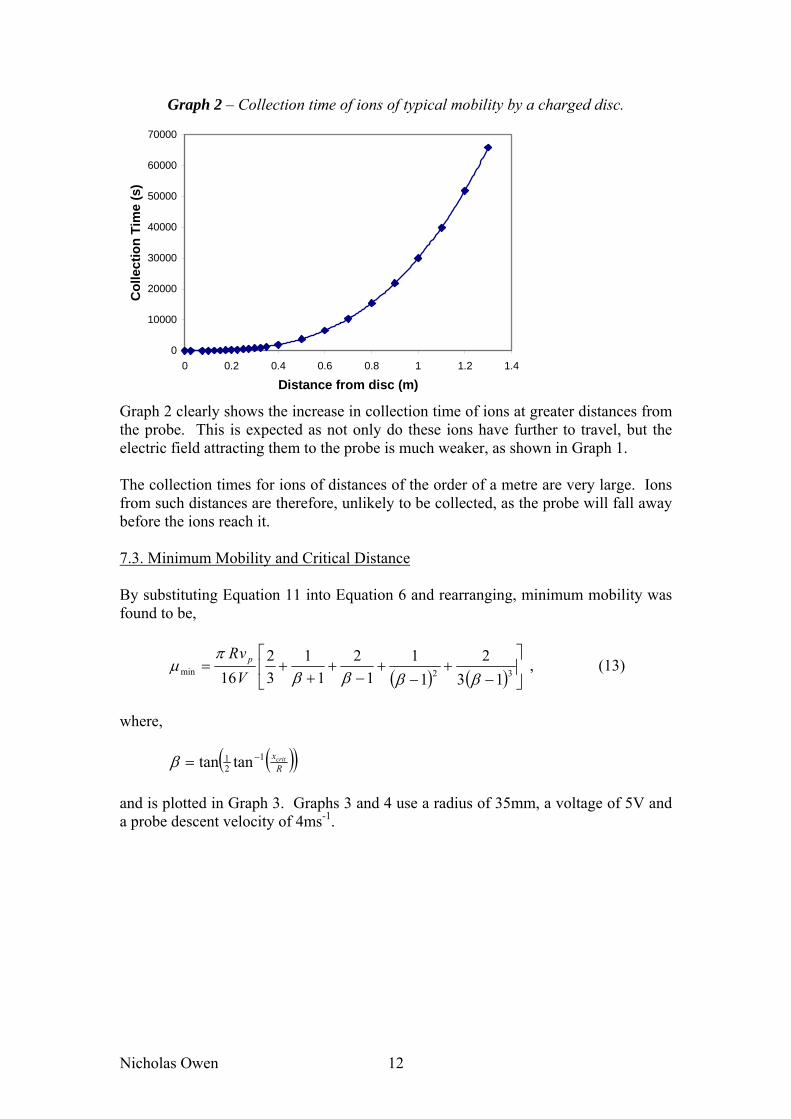
Graph 2 – Collection time of ions of typical mobility by a charged disc.

0

10000

20000

30000

40000

50000

60000

70000

0 0.2 0.4 0.6 0.8 1 1.2 1.4

Distance from disc (m)

Col

lect

ion

Tim

e (s

)

Graph 2 clearly shows the increase in collection time of ions at greater distances from the probe. This is expected as not only do these ions have further to travel, but the electric field attracting them to the probe is much weaker, as shown in Graph 1. The collection times for ions of distances of the order of a metre are very large. Ions from such distances are therefore, unlikely to be collected, as the probe will fall away before the ions reach it. 7.3. Minimum Mobility and Critical Distance By substituting Equation 11 into Equation 6 and rearranging, minimum mobility was found to be,

( ) ( ) ⎥⎦

⎤⎢⎣

⎡

−+

−+

−+

++= 32min 13

21

11

21

132

16 ββββπ

µVvR p , (13)

where, ( )( )R

xcrit121 tantan −=β

and is plotted in Graph 3. Graphs 3 and 4 use a radius of 35mm, a voltage of 5V and a probe descent velocity of 4ms-1.

Nicholas Owen 12

Graph 3 – Minimum mobility of ions collected by a charged disc at a critical distance from the disc.

0

100

200

300

400

500

600

700

800

900

1000

0 0.2 0.4 0.6 0.8 1 1.2 1.4

Critical Distance (m)

Min

imum

Mob

ility

(m²/

Vs)

As expected, the greater the critical distance the higher the mobility of ion required in order to be collected. The mobility range shown in Graph 3 is much greater than that of typical values for atmospheric ions. Graph 4, therefore, shows the critical distance for a typical range of ion mobility.

Graph 4 – For a range of typical ion mobility, the critical distance and associated minimum mobility of collected ions is plotted.

0.00

0.20

0.40

0.60

0.80

1.00

1.20

1.40

0 0.1 0.2 0.3 0.4 0.5 0.6

Critical Distance (mm)

Min

imum

Mob

ility

(cm

²/Vm

)

The critical distance and therefore, the region in which ions are collected from is very small. Ions of mobility 1 cm2V-1s-1 (10-4 m2V-1s-1) will only be collected if they lay within 0.4 mm of the relaxation probe. In reality the collection region will become even smaller than this as the voltage on the disc will decrease due to collected ions reducing the disc charge.

Nicholas Owen 13

8. Future Work The next step is to define a critical mobility for the disc. This will be done using the critical distance and minimum mobility concept. The collection of higher mobility ions from distance greater than that of the critical distance must be considered. Consideration of the voltage decay is required. The disc voltage will decay as ions are collected and so the collection time and region will change. Once critical mobility has been defined for the simplified case the generalised electric field must be found and applied. Random collisions due to thermal motion and turbulence of the atmospheric ions on Titan must be accounted for in the voltage decay. The ions below the probe will all be collected if they have the opposite parity of charge to the probe, as it will simply fall on them. This will include multiply charged ions, which have too low a mobility to be collected otherwise.

Positive ions repelled

Falling disc

Figure 10 – Collection for positively and negatively charged ions directly below falling disc.

Some ions of the same charge parity will be collected from below the falling probe, despite electric repulsion. Ions of high mobility will escape, whereas lower mobility ions will be collected. Multiply charged ions have lower mobility than singly charged ions and so are most likely to be collected in this way. The voltage decay will therefore be affected and so these effects must be found and removed from the voltage decay, reflecting the true decay from ions of appropriate mobility. The orientation of the disc will be considered, as the tilted booms will reduce the effective horizontal area. The final stage of the project is to apply the definition of critical mobility and other effects to the inversion technique in order to find mobility spectra from voltage decay data. 8.1 Project Plan Calculating the electric field for the charged disc is much more mathematically complex than first realised and so has taken longer than expected. This means that due to time restraints the application of the project wok on the Huygens data is unlikely. Therefore, the preliminary computer programme, which was proposed to be written in the first term and updated at the end of the second, has not been created.

Nicholas Owen 14

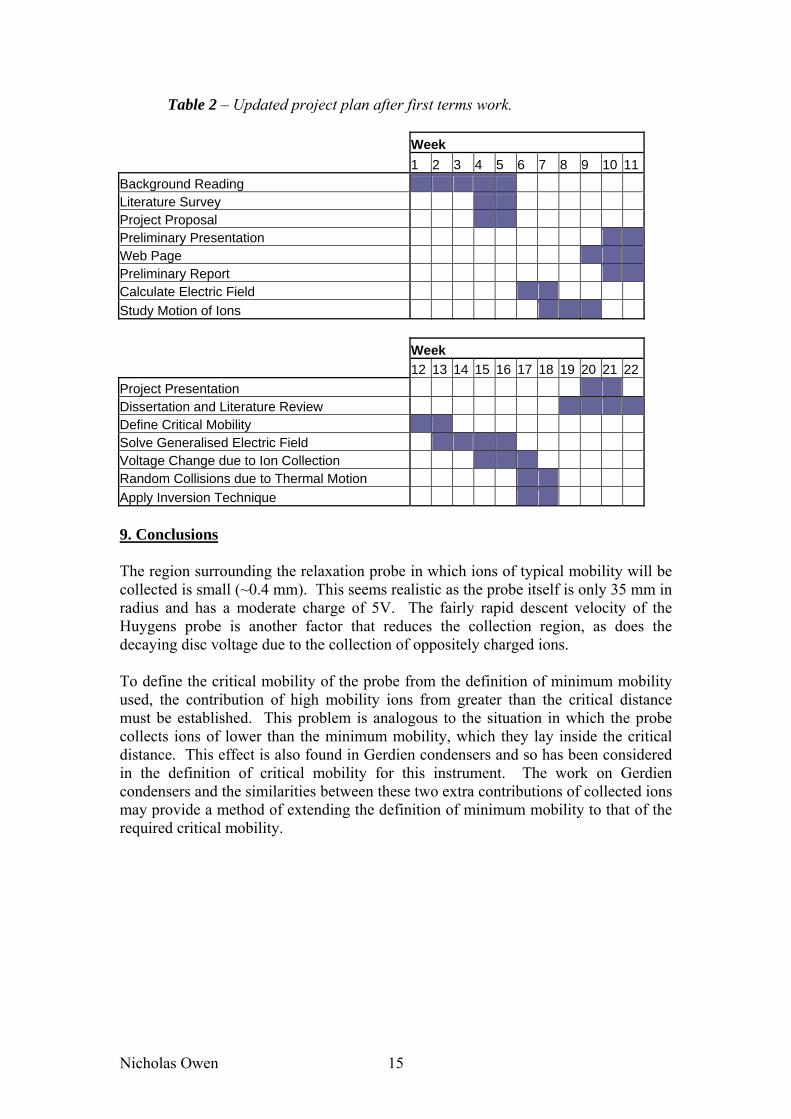
Table 2 – Updated project plan after first terms work. Week 1 2 3 4 5 6 7 8 9 10 11 Background Reading Literature Survey Project Proposal Preliminary Presentation Web Page Preliminary Report Calculate Electric Field Study Motion of Ions Week 12 13 14 15 16 17 18 19 20 21 22 Project Presentation Dissertation and Literature Review Define Critical Mobility Solve Generalised Electric Field Voltage Change due to Ion Collection Random Collisions due to Thermal Motion Apply Inversion Technique 9. Conclusions The region surrounding the relaxation probe in which ions of typical mobility will be collected is small (~0.4 mm). This seems realistic as the probe itself is only 35 mm in radius and has a moderate charge of 5V. The fairly rapid descent velocity of the Huygens probe is another factor that reduces the collection region, as does the decaying disc voltage due to the collection of oppositely charged ions. To define the critical mobility of the probe from the definition of minimum mobility used, the contribution of high mobility ions from greater than the critical distance must be established. This problem is analogous to the situation in which the probe collects ions of lower than the minimum mobility, which they lay inside the critical distance. This effect is also found in Gerdien condensers and so has been considered in the definition of critical mobility for this instrument. The work on Gerdien condensers and the similarities between these two extra contributions of collected ions may provide a method of extending the definition of minimum mobility to that of the required critical mobility.

Nicholas Owen 15

10. References Aplin, K.L. 2003, Atmospheric Ion Spectra and the rate of Voltage Decay of an Aspirated Cylinder Capacitor, Inst. Phys. Conf. Ser. No 178, Section 4. Aplin, K.L. 2005a, Aspirated Capacitor Measurements of Air Conductivity and Ion Mobility Spectra, Review of Scientific Instruments 76, 104501. Aplin, K.L. 2005b, Atmospheric Electrification in the Solar System, Surveys in Geophysics, in press. Bird, M.K. et al. 1997, The Huygens Doppler Wind Experiment, ESA Publications Division, SP-1177, p139. Freedman, R.A. and Kaufmann, W.J. 2002, Universe, New York, Sixth edition, p181. Fulchignoni, M. et al. 1997, The Huygens Atmospheric Surface Instrument, ESA Publications Division, SP-1177, p163. Harrison, R.G. and Carslaw, K.S. 2003, Ion-aerosol-cloud Processes in the Lower Atmosphere, Reviews of Geophysics. 41, 3, 1012. Israel, G. et al. 1997, The Aerosol Collector Pyrolyser Experiment for Huygens, ESA Publications Division, SP-1177, p59. Lorenz, R. 2002, Titans’ Atmosphere – A Review, J. de Phys. IV 101(10). Molina-Cuberos, G.J et al. 2002, Nitriles Produced by Ion Chemistry in the Lower Ionosphere of Titan, J. Geophys. Res. 107, E11, 5099. MacGorman, D.R. and Rust, W.D. 1998, The Electrical Nature of Storms, Oxford University Press. Niemann, H. et al. 1997, The Gas Chromatograph Mass Spectrometer Aboard Huygens, ESA Publications Division, SP-1177, p85. Owen, T. et al. 1997, The Relevance of Titan and Cassini / Huygens to Pre-biotic Chemistry and the Origin of Life on Earth, ESA Publications Division, SP-1177, p231. Tomasko, M.G. et al. 1997, The Descent Imager / Spectral Radiometer Aboard Huygens, ESA Publications Division, SP-1177, p109. Wilson, C.T.R. 1920, Investigations on lightning discharges and on the electric field of thunderstorms, Phil. Trans. Roy. Soc. London, A, 221, p73-115. Zarnecki, J.C et al. 1997, The Huygens Surface Science Package, ESA Publications Division, SP-1177, p177.

Nicholas Owen 16

Appendix 1 – Calculation of Electric Field 1.1. Calculation of x-component of Electric Field From Figure 7,

( )22 rlxs −+= , drrddq θλ= , the unit vector of s in the x direction is given by,

sxs == αcosˆ .

Substituting into Equation 3 gives,

ssdqkdE ˆ2= , (3)

( )( )( )322 rlx

xdrrdkdEx

−+=

θλ ,

( )( )( )∫∫−+

=R

x

rlx

drrdxkE0

322

2

0

π

θλ ,

( )( )( )∫

−+=

R

x

rlx

drrxkE0

3222 λπ . (7)

1.2. Calculation of radial component of Electric Field The unit vector of s in the radial direction is given by,

s

rls −== αsinˆ ,

which gives the r component of electric field,

( )( )( )( )322 rlx

rldrrdkdEr

−+

−=

θλ ,

( )( )( )( )∫∫

−+

−=

R

r

rlx

drrlrdkE0

322

2

0

π

θλ ,

( )( )( )( )∫

−+

−=

R

r

rlx

drrlrkE0

3222 λπ . (8)

Nicholas Owen 17

1.3. Calculation of Electric Field on x-axis

There is no radial component due to symmetry.

Substituting l = 0 into Equation 7 gives,

( )( )∫+

=R

axis

rx

drrxkE0

3222 λπ ,

which is integrated to,

⎟⎟⎠

⎞⎜⎜⎝

⎛+

+

−=

xRxxkEaxis

11222

λπ ,

⎟⎟⎠

⎞⎜⎜⎝

⎛

+−=

2212

RxxkEaxis λπ . (i)

Charge density and the Coulomb constant can be expressed by Equations ii and iii respectively,

RV

πε

λ 08= , (ii)

041

πε=k , (iii)

Therefore, Equation i can be expressed as,

⎟⎟⎠

⎞⎜⎜⎝

⎛

+−=

2214

Rx

xRVEaxis π

. (9)

Nicholas Owen 18

Appendix 2 – Calculation of Ion Collection Time 2.1. Ion Motion due to Mobility The mobility of an ion is defined using drift velocity in an electric field, and is expressed as,

Edtdx µ= , (4)

By rearranging Equation 4,

∫∫ =0

0

1

x

t

Edxdt

c

µ , (iv)

Assuming disc voltage is not a function of time and by substituting Equation 9 into iv an expression for the ion collection time is found,

∫+

−=

0

2214 x

c

Rxx

dxVRtµ

π (10)

2.2. Integrating Collection Time Expression To find the collection time of ions the expression,

∫+

−

0

221x

Rxx

dx ,

must be integrated. This expression can be simplified to,

( )∫∫⎟⎠⎞

⎜⎝⎛−

−=

+−

0

tan

2

0

221

sin1cos1Rxx

dR

Rxx

dxθθ

θ , (v)

by using the substitution, θtanRx = . 2.3. Partial Fractions Equation v can be expressed as a polynomial using, θsin=u , (vi)

Nicholas Owen 19

and therefore, , 22 1cos u−=θ which gives,

( ) ( )( )22 111

sin1cos1

uu −−=

− θθ ,

This can be split into the following partial fractions,

( )( ) ( ) ( ) ( )22 121

141

141

111

uuuuu −+

−+

+=

−− , (vii)

By substituting Equations vi and vii into Equation v,

( ) ( )θ

θθθθθθ dRdR

Rx

Rx

∫∫⎟⎠⎞

⎜⎝⎛

⎟⎠⎞

⎜⎝⎛ −−

⎟⎟⎠

⎞⎜⎜⎝

⎛

−+

−+

+=

−

0

tan

2

0

tan

211

sin12

sin11

sin11

4sin1cos ,

(viii) 2.4. Integration using Tan Half Angle Substitution Equation viii can be split into the following three integrals,

∫⎟⎠⎞

⎜⎝⎛−

+

0

tan 1sin1

Rx

dθ

θ , (a)

∫⎟⎠⎞

⎜⎝⎛−

−

0

tan 1sin1

Rx

dθ

θ , (b)

( )∫

⎟⎠⎞

⎜⎝⎛−

−

0

tan

21

sin12

Rx

dθ

θ , (c)

Integrals a, b and c can be solved by using the substitution,

⎟⎠⎞

⎜⎝⎛=

2tan θt , (ix)

Using this substitution, the following expressions can be found,

212

tdtd

+=θ , (x)

Nicholas Owen 20

212sin

tt

+=θ , (xi)

Therefore, (a) can be integrated,

( )∫∫

⎟⎟⎠

⎞⎜⎜⎝

⎛⎟⎠⎞

⎜⎝⎛⎟

⎠⎞

⎜⎝⎛ −−

+=

+

0

tan21

tan

2

0

tan 111

2sin1

Rx

Rx t

dtdθ

θ ,

0

tan21tan 11

2

⎟⎟⎠

⎞⎜⎜⎝

⎛⎟⎠⎞

⎜⎝⎛−

⎥⎦⎤

⎢⎣⎡

+−

=Rxt

,

( )( ) 21tantan

21

21

−+

= −Rx

, (xii)

Using Equations ix, x and xi, integral (b) is found to be,

( )∫∫

⎟⎟⎠

⎞⎜⎜⎝

⎛⎟⎠⎞

⎜⎝⎛⎟

⎠⎞

⎜⎝⎛ −−

−=

−

0

tan21tan

2

0

tan 111

2sin1

Rx

Rx t

dtdθ

θ ,

0

tan21tan 11

2

⎟⎟⎠

⎞⎜⎜⎝

⎛⎟⎠⎞

⎜⎝⎛−

⎥⎦⎤

⎢⎣⎡

−−

=Rxt

,

( )( ) 1tantan22 1

21 −

+= −Rx

(xiii)

The same process is used once again, for integral (c), which gives,

( )

∫∫⎟⎟⎠

⎞⎜⎜⎝

⎛⎟⎠⎞

⎜⎝⎛⎟

⎠⎞

⎜⎝⎛ −− ⎟

⎠⎞

⎜⎝⎛

+−+

=−

0

tan21tan

2

22

0

tan

211

1211

2)sin1(

Rx

Rx

ttt

dtdθ

θ ,

This can be simplified and partial fractions found,

( )

( )( ) ( ) ( ) ( )4324

2

2

22 1

41

41

21

12

1211

2−

+−

+−

=−

+=

⎟⎠⎞

⎜⎝⎛

+−+

ttttt

ttt

,

Which can then be integrated to get,

( )( ) ( ) ( )

0

tan21tan

32

0

tan21

tan 2 11

2

134

12

12

1211

2

⎟⎟⎠

⎞⎜⎜⎝

⎛⎟⎠⎞

⎜⎝⎛

⎟⎟⎠

⎞⎜⎜⎝

⎛⎟⎠⎞

⎜⎝⎛ −

−

⎥⎦

⎤⎢⎣

⎡

−−

−−

−−

=

⎟⎟⎠

⎞⎜⎜⎝

⎛

+−−

∫Rx

Rx ttt

ttt

dt ,

Nicholas Owen 21

( )( ) ( )( )( ) ( )( )( ) ⎟⎟

⎠

⎞

⎜⎜

⎝

⎛

−+

−+

−+=

−−− 312121

211

21 1tantan3

21tantan

11tantan

1322

Rx

Rx

Rx

.

(xiv) 2.5. Combining Integrals By combining Equations xii, xiii and xiv,

( ) ( )θ

θθθθθθ dRdR

Rx

Rx

∫∫⎟⎠⎞

⎜⎝⎛

⎟⎠⎞

⎜⎝⎛ −−

⎟⎟⎠

⎞⎜⎜⎝

⎛

−+

−+

+=

−

0

tan

2

0

tan

211

sin12

sin11

sin11

4sin1cos,

( )( ) ( )( ) ( )( )( ) ( )( )( ) ⎥⎥⎦

⎤

⎢⎢⎣

⎡

−+

−+

−+

++=

−−−− 312121

211

211

21 1tantan3

21tantan

11tantan

21tantan

132

2Rx

Rx

Rx

Rx

R

Hence, using Equation 10,

( )( ) ( )( ) ( )( )( ) ( )( )( ) ⎥⎥⎦

⎤

⎢⎢⎣

⎡

−+

−+

−+

++=

−−−− 312121

211

211

21

2

1tantan32

1tantan1

1tantan2

1tantan1

32

8Rx

Rx

Rx

Rxc V

Rtµ

π

This becomes,

( ) ( ) ⎥

⎦

⎤⎢⎣

⎡

−+

−+

−+

++= 32

2

132

11

12

11

32

8 ββββµπ

VRtc (11)

by substituting Equation 12, ( )( )R

x121 tantan −=β , (12)

Nicholas Owen 22