UNIVERSITY of CALIFORNIASANTA CRUZ

CHAOTIC MOTION IN A FORCED AND DAMPENED PENDULUM

A thesis submitted in partial satisfaction of therequirements for the degree of

BACHELOR OF SCIENCE

in

APPLIED PHYSICS

by

Aditya KunapuliSenior Thesis

University of California, Santa Cruz

May 31, 2010

The thesis of Aditya KunapuliSenior Thesis

University of California, Santa Cruz is approved by:

Professor Fred KuttnerAdvisor

Professor Fred KuttnerSenior Theses Coordinator

Professor David P. BelangerChair, Department of Physics

Abstract

CHAOTIC MOTION IN A FORCED AND DAMPENED PENDULUM

by

Aditya Kunapuli

Senior Thesis

University of California, Santa Cruz

The archetypal example of a non-linear dynamical system that can lead to chaos is

the forced pendulum in a parasitic medium. This paper explores the route to chaos

of a pendulum in air, as the drag resistance is varied. For a Q-factor between one

and 2.6, the pendulum went through two well-defined regions of period-doubling

bifurcations. The period-doubling behavior and chaos was observed through the use

of bifurcation diagrams, Poincaré maps, and Lyapunov exponents.

3

Contents

0.1 Introduction . . . . . . . . . . . . . . . . . . . . . . . . . . . . . . . . . . . . 40.2 The Non-Linear Pendulum . . . . . . . . . . . . . . . . . . . . . . . . . . . 60.3 The Route To Chaos . . . . . . . . . . . . . . . . . . . . . . . . . . . . . . . 90.4 Bifurcation Diagram . . . . . . . . . . . . . . . . . . . . . . . . . . . . . . . 10

0.4.1 Period-Doubling . . . . . . . . . . . . . . . . . . . . . . . . . . . . . 120.4.2 Chaos . . . . . . . . . . . . . . . . . . . . . . . . . . . . . . . . . . . 140.4.3 Island of Stability . . . . . . . . . . . . . . . . . . . . . . . . . . . . 15

0.5 Lyapunov Exponent . . . . . . . . . . . . . . . . . . . . . . . . . . . . . . . 160.6 Conclusion . . . . . . . . . . . . . . . . . . . . . . . . . . . . . . . . . . . . . 180.7 Appendix: Mathematica Code . . . . . . . . . . . . . . . . . . . . . . . . . 20

0.7.1 Bifurcation Diagrams . . . . . . . . . . . . . . . . . . . . . . . . . . 200.7.2 Poincaré Sections . . . . . . . . . . . . . . . . . . . . . . . . . . . . 220.7.3 Lyapunov Exponent Diagram . . . . . . . . . . . . . . . . . . . . . 240.7.4 Pendulum Animation . . . . . . . . . . . . . . . . . . . . . . . . . . 25

0.8 References . . . . . . . . . . . . . . . . . . . . . . . . . . . . . . . . . . . . . 26

0.1 Introduction

Chaos theory is the study of highly deterministic non-linear systems–i.e.non-

linear systems that are sensitive to initial conditions. A system is characterized as

chaotic if it meets certain criteria such as exhibiting an exponential rate of period

doubling in its return map, or possessing a positive Lyapunov exponent.

Chaotic behavior is observed in many systems that we interact with on a daily

basis. Examples include:

• The stock market’s volatility to bad news is just one of the many signs that

point to a chaotic system.

• The trajectory of the planets in the Solar System.1

• The weather system is highly deterministic and a classical example of chaos

in nature.

There exist many more such examples, enough so that one can make the bold

claim that chaotic systems are more common than non-chaotic systems. At least

some of this is due to the fact that the cardinality of the non-linear systems in day-

to-day life is far greater than that of linear systems. Take for example, the events

1Laskar, J. "Chaos in the Solar System." Astronomie et SystSmes Dynamiques e. (2003): n. pag.Web. 10 May, 2010.

involved with linearly accelerating a car from v0 to v1. Despite the linear accelera-

tion, both gas mileage and power consumption respond in a non-linear fashion–the

power required to keep the vehicle at v1 is primarily a function of the air resistance.

As air resistance is proportional to the square of velocity, we have that the power

consumption is a non-linear function of velocity(it is in fact proportional to the cube

of velocity)2 ,and as the gas mileage is a function of power consumption, the gas

mileage is also non-linear. Hence,chaos is not some abstract physical construct, but

rather a defining law of life and nature.

2Fuhs, Allen. Hybrid Vehicles and the future of personal transportation. CRC, 2008, 80. Print

0.2 The Non-Linear Pendulum

The dynamical system in study here is a single point-mass pendulum (of mass

m), hung from a frictionless pivot via a massless rigid tether of length l. The pen-

dulum is free to move under the force of gravity. Figure 0.1 shows the initial setup.

Figure 0.1: Simple Pendulum.

As such the Eq. of motion for this system is

mld2θ

dt2 +mgsinθ = 0. (0.1)

If we were to assume that the pendulum is contained in a viscous medium (such

as air), then using Stoke’s Law 3, we can take into account the force of air resistance.

As we are dealing with low angular velocities, the drag force will be proportional to

the angular velocity of the pendulum. Hence, Eq. (0.1) can be rewritten in the

3Cencini, Massimo, Fabio Cecconi, and Angelo Vulpiani. Chaos. World Scientific Publishing Com-pany, 2009. 5. Print.

following form

mld2θ

dt2 +mgsinθ+µdθdt

= 0. (0.2)

Where µ is the coefficient of viscosity.

As the pendulum is now dampened, all initial oscillations will eventually come

to a stop. As such, we introduce a external sinusoidal driving force. Equation (0.2)

can now be written in its final form.

mld2θ

dt2 +mgsinθ+µdθdt

= A cosωt. (0.3)

Where A is the magnitude of the driving force, and ω is the driving frequency. We

make the following substitutions in order to normalize Eq. (0.3):

t =ω0t (0.4)

ω0 =√

gl

(0.5)

ω= ω

ω0(0.6)

A = Amg

(0.7)

Q = mgω0µ

(0.8)

The normalized form of Eq. (0.3) is now

d2θ

dt2 + 1Q

dθdt

+sinθ = A cosωt. (0.9)

Within Eq. (0.9) we have that Q is known as the quality factor (Q-factor). It’s

primary purpose is to simulate a drag force on the pendulum.

0.3 The Route To Chaos

We begin investigating the route to chaos by varying the Q-factor and observing

the system’s response. A small Q-factor can sufficiently limit the pendulum’s am-

plitude such that small-angle approximations can be made in Eq. (0.9). For small

Q-factors the system begins to act in a linear fashion. Alternatively, as the Q-factor

is made larger, the system’s response should become increasing non-linear as the

amplitude increases and the small-angle approximation becomes imprecise.

The route to chaos is observed with the aide of bifurcation diagrams, Poincaré

sections, and Lyapunov exponents. The bifurcation diagrams help us observe asymp-

totic period doubling behavior. The Poincaré sections show us the phase-space tra-

jectories of the pendulum. The Lyapunov exponents give us a quantitative indicator

chaos.

0.4 Bifurcation Diagram

For the sake of uniformity, and without loss of generality we set A = 1.5, and

ω= 23 . In order to see a clear route to chaos, a bifurcation diagram of the system is

useful. Figure 0.2 shows the bifurcation diagram of the system with the previous

coefficients and with the initial conditions θ(0)= 0 and θ′(0)= 0.

Figure 0.2: Bifurcation Diagram.

From Fig. 0.2, we can see that the region beyond Q = 2.6 is chaotic. As we are

primarily interested in the period-doubling behavior of the system, we zoom in on

the region where 1.34<Q < 1.41.

Figure 0.3: Bifurcation Diagram (1.34<Q < 1.38).

The first four solid colored lines in Fig. 0.3 mark the points where period-

doubling occurs. Note the accelerated rate of doubling–this is an indicator of the

route to chaos. The dashed black line marks the point where the system transitions

to chaos. The blue line represents an island of stability. Table 1 contains the points

at which the period-doubling is readily observable.

Line Q-Value ∆Q Period<1.34 1

Red 1.347 0 2Orange 1.370 0.023 4Green 1.3745 0.004 8Purple 1.3755 0.001 8

We note that the space between successive period-doubling points is decreasing.

Comparing Fig. 0.2 and Fig. 0.3, we observe a pattern similar to that of Fig. 0.3

emerging at the tail end of the bifurcation diagram in Fig. 0.2.

0.4.1 Period-Doubling

Red Line

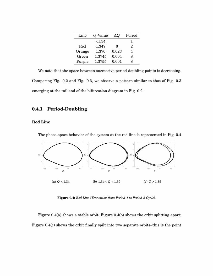
The phase-space behavior of the system at the red line is represented in Fig. 0.4

-1.0 -0.5 0.0 0.5

-1

0

1

2

Θ

Ω

(a) Q < 1.34

-1.0 -0.5 0.0 0.5

-1

0

1

2

Θ

Ω

(b) 1.34<Q < 1.35

-1.0 -0.5 0.0 0.5-2

-1

0

1

2

Θ

Ω

(c) Q > 1.35

Figure 0.4: Red Line (Transition from Period-1 to Period-2 Cycle).

Figure 0.4(a) shows a stable orbit; Figure 0.4(b) shows the orbit splitting apart;

Figure 0.4(c) shows the orbit finally spilt into two separate orbits–this is the point

where the system now posses a period-2 orbit cycle. Note that the orbit in Fig. 0.4(a)

is the same orbit as exhibited by the driving force–i.e. the system has settled into a

steady-state solution in-phase with the driving force.

Orange Line

-1.0 -0.5 0.0 0.5

-1

0

1

2

Θ

Ω

(a) 1.35<Q < 1.369

-1.0 -0.5 0.0 0.5

-2

-1

0

1

2

Θ

Ω

(b) 1.369<Q < 1.371

-1.0 -0.5 0.0 0.5

-2

-1

0

1

2

Θ

Ω

(c) 1.371<Q < 1.374

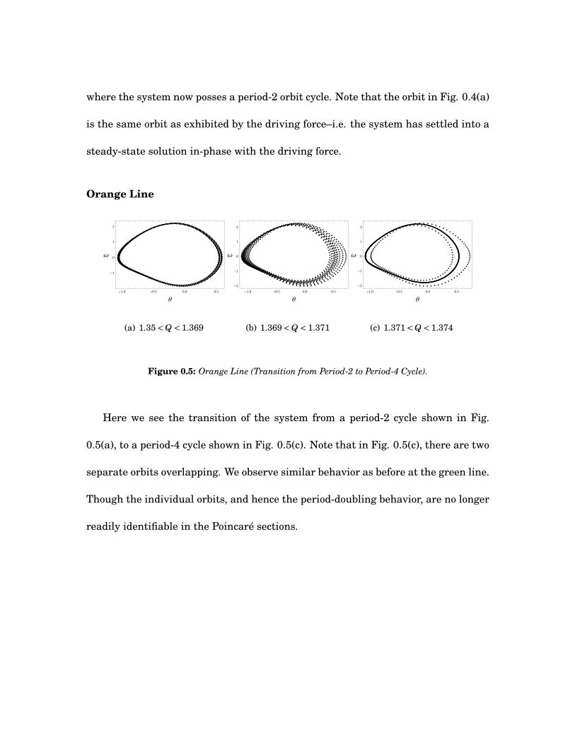
Figure 0.5: Orange Line (Transition from Period-2 to Period-4 Cycle).

Here we see the transition of the system from a period-2 cycle shown in Fig.

0.5(a), to a period-4 cycle shown in Fig. 0.5(c). Note that in Fig. 0.5(c), there are two

separate orbits overlapping. We observe similar behavior as before at the green line.

Though the individual orbits, and hence the period-doubling behavior, are no longer

readily identifiable in the Poincaré sections.

0.4.2 Chaos

From the bifurcation diagram, it may seem that beyond the purple line the sys-

tem has become chaotic, but this is in fact not the case. The system becomes chaotic

at Q = 1.405 (represented by the dashed black line in Fig. 0.3). This is not clearly

shown in the bifurcation diagram.

The Poincaré section and trajectory of the system as it transitions into chaos is

given by Fig. 0.6. Typical of such systems, the transition into chaotic behavior is

almost instantaneous–note the small difference in Q-factors between the figures.

-1.0 -0.5 0.0 0.5 1.0

-2

-1

0

1

2

Θ

Ω

(a) Q = 1.4044

-1.0 -0.5 0.0 0.5 1.0-2

-1

0

1

2

Θ

Ω

(b) Q = 1.4047

-1 0 1 2 3 4 5

-2

-1

0

1

2

Θ

Ω

(c) Q = 1.4050

20 40 60 80 100

-1.0

-0.5

0.0

0.5

1.0

t

Ω

(d) Q = 1.4044

20 40 60 80 100

-1.0

-0.5

0.0

0.5

1.0

t

Ω

(e) Q = 1.4047

20 40 60 80 100-15

-10

-5

0

t

Ω

(f) Q = 1.4050

Figure 0.6: Dashed black line (Transition to chaotic behavior).

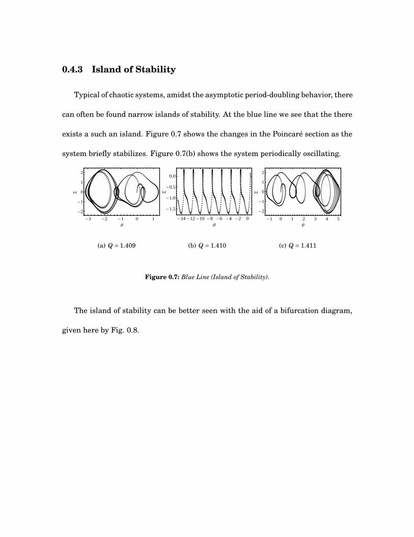
0.4.3 Island of Stability

Typical of chaotic systems, amidst the asymptotic period-doubling behavior, there

can often be found narrow islands of stability. At the blue line we see that the there

exists a such an island. Figure 0.7 shows the changes in the Poincaré section as the

system briefly stabilizes. Figure 0.7(b) shows the system periodically oscillating.

-3 -2 -1 0 1

-2

-1

0

1

2

Θ

Ω

(a) Q = 1.409

-14 -12 -10 -8 -6 -4 -2 0

-1.5

-1.0

-0.5

0.0

Θ

Ω

(b) Q = 1.410

-1 0 1 2 3 4 5

-2

-1

0

1

2

Θ

Ω

(c) Q = 1.411

Figure 0.7: Blue Line (Island of Stability).

The island of stability can be better seen with the aid of a bifurcation diagram,

given here by Fig. 0.8.

Figure 0.8: Island of Stability.

0.5 Lyapunov Exponent

The ideal method of observing the route to chaos is with the aide of a Lyapunov

diagram. The Lyapunov diagram plots the Lyapunov exponents as a function of

the Q-factor. Briefly put, when the Lyapunov exponent is negative, the system is

stable–when the Lyapunov exponent becomes positive, the system is likely to be-

come chaotic. Figure 0.9 shows the complete Lyapunov diagram of the pendulum.

Figure 0.9: Lyapunov Exponent.

More interestingly, the superposition of the Bifurcation and the Lyapunov di-

agrams (given here by Fig. 0.10) yields expected results. In the regions of clear

chaotic behavior, the system overlaps with the Bifurcation diagram.

Figure 0.10: Superposition of the Bifurcation and the Lyapunov Diagrams. The Lyapunov diagram is

given here in red. The horizontal dashed line signifies the horizontal axis.

0.6 Conclusion

Hence, we have seen that for a small Q-factor, the system’s behavior can vary

remarkably for small changes in the Q-factor. This can be interpreted to mean

that small changes in drag force can significantly affect the pendulum’s angular

frequency. This conclusion is somewhat counter-intuitive. Though the situation is

akin to the example of a passenger plane hitting a volume of low-density air–the

plane momentarily plummets. This simulation was carried out with rough approx-

imations of the actual forces involved, and with constant initial conditions. If we

were to allow the initial conditions to vary, and include a more realistic approxima-

tion of the drag force on a pendulum bob, we can expect that the route to chaos to

become shorter and more drastic.

0.7 Appendix: Mathematica Code

0.7.1 Bifurcation Diagrams

1 omega0 = 2/3;

2 A = 1.5;

3 tmin = 300;

4 nmax = 40;

5 Clear[phi , theta , omega]

6

7 soln[Q_, tmax_ , theta0_] := NDSolve [

8 phi ’[t] == omega0 , theta ’[t] == omega[t],

9 omega ’[t] == -omega[t]/Q - Sin[theta[t]] + A Cos[phi[t]],

10 phi [0] == 0,

11 theta [0] == theta0 ,

12 omega [0] == 0

13 , phi , theta , omega, t, 0, tmax]

14

15 step[Q_] := Module [nmin , temp , tmax , table , n,

16 tmax = tmin + (nmax - 1) ;

17 nmin = IntegerPart[tmin];

18 solt= soln[Q, tmax , theta0 ][[1]];

19 Table[Evaluate [Q, omega[n] /. solt], n, nmin ,

20 nmin + nmax - 1]]

21 theta0 = 0;

22 min = 1.0;

23 res = 1/1000;

24 nmax = 2000;

25 bif= step[min];

26 Do[ bstep = step[min + n *res],

27 bif= Join[bif , bstep], n, 1,

28 nmax ]; ListPlot[bif ,

29 PlotStyle -> AbsolutePointSize [1], Black,

30 FrameLabel -> Style["Q", FontSize -> 16],

31 Style [" Omega", FontSize -> 16], RotateLabel -> False ,

32 Frame -> True , Axes -> False , PlotRange -> All]

0.7.2 Poincaré Sections

Large View

1 Clear ["Global ‘*"];

2 TFINAL = 100;

3 A = 1.5;

4 Omega = 2/3;

5 Thetaprime0 = 0;

6 Theta0 = 0;

7 Q = 1.3795;

8 soln = NDSolve [Theta ’’[t] + 1/Q Theta ’[t] + Sin[Theta[t]] ==

9 A Cos[Omega*t], Theta ’[0] == Thetaprime0 , Theta[

10 0] == Theta0, Theta[t], t, 0, TFINAL ][[1]];

11 Theta[t_] = Theta[t] /. soln;

12 v[t_] = Theta ’[t];

13 ListPlot[Drop[Table[Theta[t]/Pi , v[t], t, 0, TFINAL , .1], 100],

14 PlotRange -> All , Frame -> True , Axes -> False ,

15 RotateLabel -> False ,

16 FrameLabel -> Style[" Theta", FontSize -> 16],

17 Style [" Omega", FontSize -> 16],

18 PlotStyle -> Black , AbsolutePointSize [3]]

Table View

1 TFINAL = 100;

2 A = 1.5;

3 Omega = 2/3;

4

5 sol[q_] :=

6 NDSolve [theta ’’[t] + 1/q theta ’[t] + Sin[theta[t]] ==

7 A Cos[Omega*t], theta ’[0] == 0, theta [0] ==

8 0, theta[t], t, 0, TFINAL ];

9 Table [q,

10 theta[t_] = theta[t] /. sol[q][[1]];

11 v[t_] = theta ’[t];

12 list = Drop[Table[theta[t]/Pi , v[t], t, 0, TFINAL , .1] ,100];

13 ListPlot[list , PlotRange -> All , Frame -> True , Axes -> False ,

14 RotateLabel -> False ,

15 FrameLabel -> Style[" theta", FontSize -> 16],

16 Style ["v", FontSize -> 16],

17 PlotStyle -> Black , AbsolutePointSize [2]] , q, 1.378,

18 1.38, .001]

0.7.3 Lyapunov Exponent Diagram

1 Clear ["Global ‘*"];

2 list = Table[

3 TFINAL = 100;

4 A = 1.5;

5 omega = 2/3;

6 T = 10;

7

8 sol[q_, nAngle_] :=

9 NDSolve [theta ’’[t] + 1/q theta ’[t] + Sin[theta[t]] ==

10 A Cos[omega*t], theta ’[0] == 0,

11 theta [0] == nAngle, theta[t], t, 0, TFINAL,

12 MaxSteps -> Infinity ][[1]];

13 nAngle = 0;

14 l = Table[

15 v = Cos[Evaluate[theta[t] /. sol[Q, nAngle] /. t -> 50]],

16 Sin[Evaluate[theta[t] /. sol[Q, nAngle] /. t -> 50]];

17 T += 10;

18 V[m] = v;

19 U[m] = V[m] - Sum[Projection[U[n], V[m]], n, 1, m - 1];

20 nAngle = Arg[U[m][[1]] + U[m][[2]] I ]*180/ Pi;

21 Log[Norm[U[m]]]

22 , m, 1, 20];

23 Q, Total[l]/( Length[l]*10) , Q, 1, 3, .001];

24 ListPlot[list , Frame -> True ,

25 PlotStyle -> Red , AbsolutePointSize [2],

26 FrameLabel -> Style["Q-Factor", FontSize -> 18],

27 Style [" Lyapunov Exponent (\!\(\* SubscriptBox [\" Lambda\", \"L\"]\

28 \))", FontSize -> 18], Axes -> False]

0.7.4 Pendulum Animation

1 Clear ["Global ‘*"];

2 TFINAL = 500;

3 A = 1.5;

4 Omega = 2/3;

5 Q = 1.4;

6 Thetaprime0 = -.75;

7 Theta0 = 1;

8 soln = NDSolve [Theta ’’[t] + 1/Q Theta ’[t] + Sin[Theta[t]] ==

9 A Cos[Omega*t], Theta ’[0] == Thetaprime0 , Theta[

10 0] == Theta0, Theta[t], t, 0, TFINAL ][[1]];

11 Theta[t_] = Theta[t] /. soln;

12 v[t_] = Theta ’[t];

13 Animate[

14 p = -Sin[Theta[t]], Cos[Theta[t]];

15 Show[Graphics [Line [0, 0, p], Disk[p, 0.1]] , Axes -> False ,

16 PlotRange -> 1.5 -1, 1, -1, 1, AspectRatio -> Automatic],

17 t, 0.1, TFINAL , 0.01, AnimationRunning -> False ,

18 AnimationRate -> 20]

0.8 References

1. Awrejcewicz, Jan, Yuriy Pyryev, and Thomas Bär. The vascular system of the

cerebral cortex. Springer, 1980. Print.

2. Greiner, Walter. Classical Mechanics. Springer Verlag, 2010. 169-170. Print.

3. Kapitaniak, Tomasz. Chaotic oscillators. World Scientific Pub Co Inc, 1992.

Print.

4. Lakshmanan, Muthusamy, and K. Murali. Chaos in nonlinear oscillators.

World Scientific Pub Co Inc, 1996. Print.

5. Lakshmanan, Muthusamy, and Shanmuganathan Rajasekar. Nonlinear dy-

namics. Springer Verlag, 2003. Print.

6. Landau, Rubin, Manuel Mejía, and Cristian Bordeianu. Computational physics.

Vch Verlagsgesellschaft Mbh, 2007. 277-310. Print.

7. Litak, Grzegorz, and et al. . "Vibration of externally-forced froude pendulum."

(1997): 11. Web. 31 May 2010.

<http://litak.pollub.pl/litak_ijbc1999_561.pdf>.

8. Sandri, Marco. "Numerical Caluclation of Lyapunov Exponents." Mathemati-

cal Journal (1996): 84. Web. 21 May 2010.

<http://library.wolfram.com/infocenter/Articles/2902/>.

9. Schuster, Heinz, and Wolfram Just. Deterministic chaos. Wiley-VCH Verlag

GmbH, 2005. Print.

10. Sriram, M.S., and K. Ramasubramanian. "Title: A comparative study of com-

putation of Lyapunov spectra with different algorithms." (2008): 25. Web. 21

May 2010.

<http://arxiv.org/abs/chao-dyn/9909029>.

11. Sun, Jian-Qiao, and Albert Luo. Bifurcation and chaos in complex systems.

Elsevier Science Ltd, 2006. 287-291. Print.

12. Taylor, John, and Peter Ryder. Classical Mechanics. Peter Ryder, 2007. 462-

465. Print.

13. Virgin, Lawrence. Introduction to experimental nonlinear dynamics. Cam-

bridge Univ Pr, 2000. Print.