Univers

ity of

Cap

e Tow

n

DEVELOPMENT OF A FINE COAL BENEFICIATION CIRCUIT FOR THE TWISTDRAAI COLLIERY

. A Thesis Submitted to the UNIVERSITY OF CAPE TOWN

in Fulfillment of the Requirements for the Degree MASTER OF SCIENCE IN APPLIED SCIENCE

by John Reginald Bunt

GDE (Coal Technology) (Wits University) NHD (Extractive Metallurgy) (Wits Technikon)

Department of Chemical Engineering University of Cape Town Rondebosch 7700 South Africa September 1997

Univers

ity of

Cap

e Tow

n

The copyright of this thesis vests in the author. No quotation from it or information derived from it is to be published without full acknowledgement of the source. The thesis is to be used for private study or non-commercial research purposes only.

Published by the University of Cape Town (UCT) in terms of the non-exclusive license granted to UCT by the author.

SYNOPSIS

Lt/ 0tao 13!..4.1'JT

Cff?/lllf-CJ

The principal aim of this thesis was to develop a fine coal beneficiation circuit for the Twistdraai Colliery capable ofachieving.a saleable 10.0% ash (28 MJ/kg CV) product. Gravity circuit testing involved a comparative study of a conventional double-stage Spiral circuit and a Stokes upward-current washer when treating Twistdraai <850J.1m x 106J.1m fine coal. In addition, froth flotation technologies, in the form of the Microcel column and the Jameson cell were also tested in order to ascertain whether they can be suitably applied · to the Twistdraai naturally fine coal to produce a 10.0% ash steam coal export product.

In this investigation, the Twistdraai fine coal surface was characterised by size as well as by density. Functional group determination included the measurement of the coals hydroxyl, carboxylic and total acid groups, since these exert the most important influence on the properties of the coal surface. These are supported by contact angle measurements, petrographic analysis and washability measurements in orde:r to determine the oil wettability of the coal fractions prior to flotation testing.

The results described and discussed in this thesis show that it was possible to recover the desired quality of product by employing split-stream processing of the (850J.1m x 0) Twistdraai fine coal circuit feed. This was achieved by application of both gravity concentration and froth flotation technologies treating specific particle size ranges.

The best yield of clean coal below 10.0% ash was obtained \Vhen employing the following circuit design: (1) Single-Stage (LD*) Spirals for de-shaling, (2) Cleaning ofthe Spiral product using the Stokes upward-current washer as a second-stage gravity cleaning device, (3) Desliming of the Stokes separator product at 300J.lm to yield a 10% ash product in the <850J.lm x 300J.lm size range and ( 4) Single-Stage froth flotation treatment of the -300J.lm x 38J.1m fraction using a Jameson cell. Combination of the Stokes separator deslimed product anq the froth flotation cell product produced a practical yield of36. 7% at 9.9% ash, which relates to an organic efficiency of96% for this circuit design.

An order-of-magnitude costing of the above mentioned fine coal circuit (incorporating a screenbowl centrifuge for product dewatering) also indicated that ~his circuit is economically attractive (20% IRR). This option was also the rriost expensive of those considered and capital to the value of R8 315 000 would be required to facilitate the required processing equipment. The analysis further indicated that froth flotation was beneficial to the economic viability of the proposed Twistdraai fine coal treatment circuit.

Froth flotation was also successfully described in terms of the Ecart probable ( epm) for both a conventional mechanical flotation cell and a Jameson flotation cell for coal sized between 850J.1m x 0 in this application. Partition numbers were both measured as well as simulated using the Zitwash coal washing simulator, and excellent agreement between the two techniques was obtained. It was found that the Jameson flotation cell (epm = 0.081) was a far more efficient separation device than the conventional mechanical cell ( epm =

0.2159).

* (LD) = Large diameter - 1000 mm

l I .

/I

11

ACKNOWLEDGEMENT

The ~uthor would like to extend his thanks to the following people and organisations for their help and assistance throughout this study: ·

SASTECH R&D for the funding of this research project. .

Prof J-P Franzidis and Mr Martin Harris ofU.C.T. for their assistance and guidance as supervisors.

Dr P van Nierop of SASTECH R&D for his constructive input and assistance as co­supervisor.

. . Mr H Hamman ofTwistdraai Colliery for the interest he showed in the test programme.

Dr M Vosloo and Mrs K Coetzee of SASTECH R&D Statistical Division for developing the experimental programme as well as the associated models.

Colleagues : V Schneider, G Tshabalala, M Keyser, M Schneider and G de Jager for their assistance in the characterisation work, pilot-scale and batch flotation equipment.

·Messrs D Hyde and :M: Lawrenson of Stokes (UK) and Eriez Magnetics respectively for . assistance during the commissioning of the Stokes separator unit.

Mr J de Korte of the C.S.I.R. for conducting the economic evaluation given in Chapter 7 of this dissertation. ·

Me M Schoeman for the typing of this manuscript text and Mr J Joubert for scanning of the thesis figures as well as for proofreading ..

My wife and family for their encouragement, interest and support.

To Him who deserves all honour.

lll

CONTENTS

CHAPTER I

INTRODUCTION

1.1 BACKGROUND

1.2 THE TWISTDRAAI EXPORT PROJECT

1.3 THESIS AIMS AND SCOPE

1.4 STRUCTURE OF THE THESIS

CHAPTER2

LITERATURE REVIEW

2.1 INTRODUCTION

2.2 COAL ORIGIN Al\TJ) CLASSIFICATION

2.3 THE COALIFICATION PROCESS

2.4 COAL COMPOSITION 2.4.1 The microscopic structure of coal

2.4 .1.1 Carbonaceous material 2.4.1.1.1 Properties of coal macerals

2.4.1.1.1.1 Physical structure 2.4.1.1.1.2 Chemical composition

2.4.1.2 Minerals present in coal 2.4.2 The macroscopic structure of coal

2.5 COAL CHARACTERISATION METHODS 2.5.1 Proximate and ultimate analysis 2.5.2 Petrographic analysis 2.5.3 Float and Sink analysis 2.5.4 Surface characterisation

2.5.4.1 Contact angles 2.5.4.2 Oxygen containing functional groups

2.5.5 Flotation release analysis

Page

1

2·

2

3

4

4

4

5 6 6 7 7 7 7 8

9 10 10 11 14 15 16 16

2.6

IV

COAL IN SOUTH AFRICA 2.6.1 The characteristics of gondwanaland coal

2.6.1.1 Petrography 2.6.1.2 JtanJc

17 17 17 18

2.6.1.3 Mineral associations 18 · 2.6.2 South African coal reserves 19

2.6.2.1 Occurance 19 2.6.3 Fine coal characteristics 21

2.6.3.1 Liberation effects offine coal 21 2.6.4 Characteristics ofhighveld number 3+4 seam coal 22

2.6.4.1 Preparation characteristics of the WitbanJc-Middelburg coalfields 23 2.6.4.2 Preparation characteristics of the Highveld coalfield 23 2.6.4.3 Characteristics ofHighveld fine coal 24

2. 7 FINE COAL BENEFICIATION 24 25 26 27 29 30 32 33 35 35 37 37 37 38 40 40 40 41 41 42 42 42 44 45 45 45 45 46

2. 7 .I Gravity concentration methods 2. 7 .I.l The concentrating table 2.7.1.2 The water-only cyclone (autogenous cyclone) 2. 7.I.3 · The dense medium cyclone 2. 7.1.4 The fine coal feldspar jig 2. 7 .1. 5 The spiral concentrator 2. 7 .1. 6 The upward current washer or hindered-bed classifier 2. 7 .1. 7 Enltanced gravity concentrators 2.7.1.8 Summary of:fine coal gravity concentrators

· 2. 7.2 Gravity concentration equipment selected 2. 7 .2.I The spiral concentrator

2. 7 .2.I.I Operating characteristics of spirals 2. 7 .2.1.2 Spiral operating parameters

2.7.2.2 Stokes upward current washer 2. 7.2.2.1 Theoretical basis of density separation 2. 7 .2.2.2 Design criteria - Stokes variables

2.7.2.2.2.I Shale cut size 2.7.2.2.2.2 Let-down rate 2.7.2.2.2.3 Upward current water

2.7.2.2.3 Pilot unit operating data 2.7.3 Separation based on the surface properties of coal

2. 7.3 .I Factors determining the floatability of coal 2.7.3.l.I Natural floatability 2.7.3.1.2 Surface functional groups 2.7.3.1.3 Slime coating and entrainment 2.7.3.1.4 Particle size distribution 2.7.3.1.5 Petrographic components 2.7.3.1.6 Frother dosage 2. 7.3 .I. 7 Collector dosage 2. 7.3 .1. 8 Temperature effects 2.7.3.1.9 Coal pulp conditioning

46 46 47 47

2.8

3.1

3.2

v

2.7.3.2 Froth flotation cells 2. 7.3 .2.1 The Mechanical Flotation cell 2.7.3.2.2 The Column cell 2.7.3.2.3 The Jameson cell 2.7.3.2.4 The Packed column 2.7.3.2.5 The Wemco/Leeds column 2.7.3.2.6 The Hydrochem Flotation column 2.7.3.2.7 The Pneumatic Flotation column 2.7.3.2.8 The Bahr cell 2.7.3.2.9 The Deister Flotaire column 2.7.3'.2.10 The Microcel Column cell 2. 7.3.2.11 Summary of froth flotation equipment

2.7.3.3 Froth flotation equipment selected 2. 7. 3. 3 .1 Microcel column operating parameter effects

2.7.3.3.1.1 Particle size 2.7.3.3.1.2· Slurry feed rate and solids content 2.7.3.3.1.3 Sparger design 2.7.3.3.1.4 Air flow rate 2.7.3.3.1.5 Wash water addition and Bias 2.7.3.3.1.6 Froth height .2. 7.3 .3 .1. 7 Frother dosage 2.7.3.3.1.8 Collector dosage

2.7.3.3.2 Jameson cell operating parameter effects 2.7.3.3.2.1 Feed pressure 2.7.3.3.2.2 Air supply to the cell 2. 7.3.3.2.3 Frother to collector ratio 2.7.3.3.2.4 Wash water addition and bias 2.7.3.3.2.5 Froth height 2.7.3.3.2.6 Particle size and feed solids concentration

FINE COAL TREATMENT PRACTICE 2.8.1 Gravity concentration circuits and practice

2.8.1.1 Spiral concentration circuits 2.8.1.2 Upward current washer circuits

2.8.2 Froth flotation circuits and practice 2.8.3 Fine coal dense medium circuit 2.8.4 Chapter Summary

CHAPTER3

EXPE~ENTALPROCEDURES

INTRODUCTION

SAMPLE CHARACTERISATION 3 .2.1 Coal used in this study

47 48 50 51 53 54 55 55 56 56 57 58 59 59 59 61 62 63 64 65 65 65 66 66 66 68 68 69 69

69 70 70 70 71 73

73b

74

74 74

3.3

3.4

3.5

3.6

4.1

4.2

VI

3 .2.1.1 Gravity concentration coal sample 3 .2.1.2 Froth flotation coal sample

COAL CHARACTERISATION TECHNIQUES 3.3 .1 Density separation (float-and-sink analysis) 3.3 .2 Flotation release analysis 3.3 .3 Surface oxidation analysis

3.3 .3 .1 · Functional group determination 3.3 .3 .1.1 Carboxylic acid groups 3.3.3.1.2 Hydroxyl groups 3.3.3.1.3 Total acid and hydroxylic acid groups

3.3.4 Contact angle and preliminary reagent screen

ANALYTICAL TECHNIQUES 3 .4 .1 Ultimate analysis 3.4 .2 Proximate analysis 3.4.3 Petrographic analysis

GRAVITY CONCENTRATION :METHODOLOGY 3.5.1 Spiral circuit 3.5 .2 Stokes upward current washer

FROTH FLOTATION METHODOLOGY 3.6.1 Batch leeds cell ·

3.6.1.1 Batch cell description 3.6.1.2 Batch cell testing using experimental designs 3. 6 .1.3 General batch cell operation

3.6.2 Microcel column cell 3. 6.2.1 Microcel column cell description 3.6.2.2 Microcel column testing using experimental designs 3.6.2.3 General microcel column operation

3.6.3 Jameson cell 3.6.3.1 Jameson cell description 3.6.3.2 Jameson cell testing using experimental designs 3.6.3.3 General jameson cell operation

3 .6.4 Double-stage flotation

CHAPTER4

RESULTS AND DISCUSSION: GRAVITY CONCENTRATION TESTS

INTRODUCTION

CHARACTERISATION RESULTS

74 75

. 75

75 76 77 77 77 78 78 79

80 80 80 80

81 . 81

81

82 82 82 83 84 84 84 86 88 89 89 91 92 92

94

94

/

Vll

4.2.1 Ultimate, proximate & petrographic analysis results 4.2.2 Single-Stage circuit feed characterisation results

4.2.2.1 Washability results 4.2.2.2 Yield:-by-size and ash-by-size results

4.2.3 Two-stage circuit feed characterisation results 4.2.3.1 Washability results 4.2.3.2 Yield-by size and ash-by-size results

94 95 95 96 97 97 98

4.3 SINGLE-STAGE CIRCUIT TEST RESULTS 100 4.3.1 Single-stage Spiral circuit results 100 4.3.2 Single-stage Stokes separator results 101 4.3.3 Comparison ofthe single-stage Spiral and Stokes separator results 101

4.4 TWO-STAGE CIRCUIT TEST RESULTS 103 4.4.1 Two-stage Spiral circuit results 103 4.4.2 Two-stage Stokes separator results 104 4.4.3 The effect ofdesliming on the two-stage circuit 104

4.5 CHAPTER SUMMARY 109

5.1

5.2

CHAPTERS

RESULTS AND DISCUSSION : FROTH FLOTATION TESTWORK

INTRODUCTION

COAL SAMPLE CHARACTERISATION RESULTS 5 .2.1 Size and ash-by-size results

5.2.1.1 Composite (850f.!m x 0) size fraction 5.2.1.2 Deslimed (300f.!m x 38f.!m) size fraction

5.2.2 Float-and-sink analysis results 5.2.3 Release flotation results

5.2.3.1 Composite (850f.!m x 0) size fraction 5.2.3.2 Deslimed (300f.!m x 38f.!m) size fraction

5.2.4 Surface oxidation results 5.2.4.1 Surface functional groups

5.2.5 Contact angle measurement results 5.2.6 Reagent screening results

5.2.6.1 Composite (850f.!m x 0) size fraction 5.2.6.2 Deslimed (300f.!m x 38f.!m) size fraction

..

111

Ill 112 112 112 113 113 113 114 115 115 116 117 117 119

5.3

5.4

Vlll

FROTH FLOTATION RESULTS 5.3 .1 Single-stage test results for the (8501lm x 0) fine coal sample

5.3 .1.1 Mechanical cell results 5. 3 .1.1.1 Global flotation results 5.3.1.1.2 Parameter effects

5.3.1.2 Microcel column cell results 5.3.1.2.1 Global flotation results 5.3.1.2.2 Parameter effects

5.3.1.3 Jameson cell results 5.3 .1.3 .1 Global flotation results 5.3 .1. 3 .2 Parameter effects

5.3.1.4 Single-stage froth flotation cell comparison (8501lm x 0) 5.3 .1. 4.1 Global comparison

5.3.2 Single-stage test results for the deslimed (300!-!m x 38!lm) coal sample

5.3.2.1 Global results 5.3.3 Two-stage test results

5.3 .3 .1 Global results 5.3.3.2 Cleaner concentrate fractional yield-by-size and ash-by-size

results 5.3.3.3 Impact ofbeneficiation of coal quality

5.3.4 Efficiency testing of froth flotation 5.3.4.1 Jameson cell measured results 5.3.4.2 Jameson cell simulation results 5.3.4.3 Mechanical cell simulation results

CHAPTER SUMMARY

CHAPTER6

RESULTS AND DISCUSSION: TWISTDRAAI FINE COAL CIRCUIT DEVELOPMENT

120 120 120 120 121 127 127 128 133 133 135 139 139 142

143 144 144 145

147 147 148 149 150

150

6.1 INTRODUCTION 152

6.2 CIRCUIT DEVELOPMENT RATIONALE 153

6.3 TWO-STAGE (LD) SPIRAL CIRCUIT 153

6.4 CIRCUIT INCLUDES: TWO STAGE (LD) SPIRALS, DESLIMING 153 AND FROTH FLOTATION

6.5 CIRCUIT INCLUDES : SINGLE-STAGE (LD) SPIRALS, STOKES 154 HYDROSIZER, DESLIMING AND FROTH FLOTATION

6.6 THE EFFECT OF PROCESS CIRCUIT CONFIGURATION ON 154 ORGANIC EFFICIENCY

IX

CHAPTER 7

RESULTS AND DISCUSSION: 159 PROPOSED TWISTDRAAI FINE COAL CIRCUIT ECONOMIC EVALUATION

7.1 INTRODUCTION 159

7.2 BOUNDARIES 159

7.3 BENEFICIATION OPTIONS 159

7.4 ASSUMPTIONS 160

7.5 CAPITAL COSTS 161

7.6 FINANCIAL VIABILITY 162

7.7 ECONOMIC RESULTS OBTAINED 162

CHAPTERS

SUMMARY AND CONCLUSIONS 164

REFERENCES 167

APPENDICES

APPENDIX A Appendix A.1 : Experimental design and analysis of results A-1 Appendix A.2 : Froth flotation experimental design programmes A-5 Appendix A.3 : Surface response data and model development A-9

APPENDIXB Appendix B 1 : Determination of the functional groups B-1 Appendix B2 : Ash content of coal (SABS Standard No 296) B-5

APPENDIXC Appendix C 1 : Process flow diagram of the Twistdraai 150tph C-1

pilot plant facility Appendix C2 : Float-and-sink data C-2 Appendix C3 : Spiral circuit data C-3 Appendix C4 : Upward-current washer data C-8

APPENDIXD Appendix D 1 : Reagent screening programme data D-1 Appendix D2 : Float-and-sink data D-6

X

Appendix D3 : Release flotation data D-7 Appendix D4 : Batch flotation data D-8 Appendix DS : Microcel column data D-10 Appendix D6 : Jameson cell data D-18 Appendix D7 : Two-stage flotation data D-29 Appendix D8 : Efficiency (epm) data· D-31

APPENDIXE Appendix El : Sample calculations E-1 Appendix E2 : Circuit mass balances E-3

X1

LIST OF TABLES Page

Table 2.1: The main chemical changes in coalification (Falcon, 1977). 5

Table 2.2: Typical maceral compositions (% by volume) of two principal 18 coal regions\. of the world (after Falcon, 1977).

Table 2.3: Separation cut-point and efficiency data as a function of particle 27 size for a Deister table (after Luckie, 1987).

Table 2.4: Separation cut-point and efficiency data as a function of particle 28 size for the water-only cyclone (after Hornsby et al, 1983).

Table 2.5: Separation cut-point and efficiency data as a function of particle 30 size for fine coal dense medium cyclones operating at the Homer city plant (after Chedgy, 1986).

Table 2.6: Separation cut-point and efficiency data as a function of patticle 32 size for-the fine coal Feldspar jig (after Killmeyer, 1980).

Table 2.7: Separation cut-point and efficiency data as a function of particle 33 size for the Spiral concentrator (after Hornsby et al, (1983).

Table 2.8: Historical Stokes upward current washer efficiency data (af1ter 35 Hyde et al, 1988).

Table 2.9: Separation cut-point and efficiency data as a function of particle 36 size for the fine coal gravity concentration devices reviewed.

Table 2.10: The operating characteristics of Spiral plants in South Africa, 1990 38 and 1995 (after Harris et al, 1995).

Table 2.11: Summary of feed parameters that can effect the Spiral separation 39 (after Mikhail et al, 1987).

Table 3.1 Constant and uncontrolled operating parameters for the 83 mechanical leeds cell.

Table 3.2: Mechanical leeds cell operating parameters. 84

Table 3.3 : Constant and uncontrolled operating parameters for the Microcel 87 column.

Table 3.4: Microcel column operating parameters. 87

xu

Table 3.5: Typical flotation column operating parameter values, from 88

(Yianatos, 1989).

Table 3.6: Constant and uncontrolled operating parameters for the 91

Jameson cell.

Table 3.7: Jameson cell operating parameters. 91

Table 4.1: Ultimate, Proximate and Petrographic analysis results for the 95 Twistdraai (850 J.lm x 106 J.lm) fine coal composite.

Table 4.2: Summary of the yield and ash distribution results obtained for 100 the single-stage Spiral results.

Table 4.3: Summary of the yield and ash distribution results obtained for 101 the single-stage Stokes separator.

Table 4.4: Summary of the yield and ash distribution results obtained for 103 the two-stage Spiral tests.

Table 4.5: Summary of the yield and ash distribution results obtained for 104 the two-stage Stokes separator.

Table 5.1 : Ash-by-Size distribution data for the composite (850J.1m x 0) 112 Twistdraai fine coal sample.

1 Table 5.2: Ash-by-Size distribution data for the deslimed (300J.1m x 38J.1m) 113

Twistdraai fine coal sample.

Table 5.3: Functional group characterisation results for Twistdraai fine coal. 115

Table 5.4: Average contact angle-by-size measurement results obtained 116 for the (850J.1m x 0) Twistdraai fine coal sample.

Table·5.5: Reagent (type and dosage) yielding less than 19% ash in the 118 reagent screening programme treating (850J.1m x 0) Twistdraai fine coal.

Table 5.6: Process conditions necessary to obtain optimum performance 125 for the Mechanical batch cell treating (850J.1m x 0) Twistdraai fine coal.

Table 5.7: Process conditions necessary to obtain optimum performance 132 for the Microcel column cell treating (850J.lm x 0) Twistdraai fine coal.

Xlll

Table 5.8: Process conditions necessary to obtain optimum performance 136 for the Jameson cell treating (850J.1m x 0) Twistdraai fine c:oal.

Table 5.9: The optimum results obtained in terms of product yield 141 and ash for the three flotation cells during single-stage operation when treating (850J.1m X 0) Twistdraai fine coal.

Table 5.10: Throughput capacity and superficial velocity results obtained 142 for the two continuous· cells when treating (850J.1m x 0) Twistdraai fine coal.

Table 5.11: Proximate, ultimate and CV analysis of the Twistdraai 147 (850J.1m x 0) feed and Jameson cell cleaner concentrate samples.

Table 7.1 Estimated installed capital cost of the items considered for the 161 proposed Twistdraai fine coal circuit.

Table 7.2 Economic results showing the capital cost, increase in 162 contribution, NPV and IRR data obtained for the four options considered.

XIV

LIST OF FIGURES Page

Figure 2.1: Example of the classical washability curves ( densimetric, 12 difficulty and cumulative ash) for a Witbank No 2 seam coal (Horsfal~ 1993).

Figure 2.2: Example of a partition curve after Horsfall, 1993. 14

Figure 2.3: Correlation between the contact angle of an oil on the coal 15 surface and the carbon content of the coal (after Aplan, 1976).

Figure 2.4: Location of the major South African coalfields 20 (after Chamber of Mines, 1981).

Figure 2.5: Scematic of a Deister "88" double-deck coal washing table. 26

Figure 2.6: Schematic of a typical water-only cyclone (autogenous 28 cyclone).

Figure 2.7: Schematic of a fine coal jig with superimposed air cycle. 31

Figure 2.8: Schematic of a typical spiral concentrator. 32

Figure 2.9: Schematic of a typical upward current washer. 34

Figure 2.10: Theoretical basis for the density separation achieved in the 40 upward current washer (after Honaker, 1996).

Figure·2.11: Cross-section of a Denver sub aeration "cell-to-cell" flotation 48 machine.

Figure 2.12: Schematic showing the adsorption of frother onto coal 49 particles (after Reinecke, 1987b).

Figure 2.13: Schematic diagram of a counter-current flotation column. 50

Figure 2.14: Schematic diagram of the Jameson cell. 52

Figure 2.15: Schematic diagram of a packed flotation column 54 '(after Yang, 1988).

Figure 2.16: Schematic diagram of a WEMCO/Leeds flotation cell 55 (after Miller, 1988).

Figure 2.17: Diagram of the Pneumatic flotation column. 56

XV

Figure 2.18: Diagram of a Microcel flotation column (after Yoon et al, 1980). 58

Figure 2.19: Floatability as a function of particle size (after Tsai, 1982). 60

Figure 2.20: Froth flotation concentrate recovery/grade distribution as 60 a function of particle size (after Tsai, 1982).

Figure 2.21: Schematic of a Microcel in-line static mixer air-sparging system (after Yoon, 1980).·

Figure 2.22: The effect ofpump speed on,the mean bubble size and volumetric hold-up (after Yoon, 1980).

Figure 2.23: Relationship between vacuum and air for the Jameson cell.

Figure 2.24: Typical flowsheet incorporating coal-cleaning Spirals.

62

63

67

70

Figure 2.25: Flowsheet showing the metallurgical performance and mass 71 flows achieved by the Floatex-packed column circuit for the treatment of -16 mesh coal.

Figure 2.26: Twin single-stage flotation treatment of a coarse and fine c:oal, 72 following pre-classification using a hydrocyclone.

Figure 2.27: Two-stage flotation circuit. 72

Figure 2.28: Simplified flowsheet of a dense medium cyclone plant. 73a

Figure 3.1 : Schematic representation of a contact angle measuring apparatus. 80

Figure 3.2: Schematic arrangement ofthe Stokes Upward Current Washer. 82

Figure 3.3 : Schematic of the Batch Leeds cell. 83

Figure 3.4: Schematic arrangement of the Microcel column and equipment. 85

Figure 3.5 : Schematic of the Jameson cell and accompanying equipment. 89

Figure 4.1 : Densimetric, difficulty and cumulative floats curves for the 95 primary-stage gravity circuit feed.

Figure 4.2: Primary Spiral circuit feed consistancy results showing cumulative 96 yield by size data for the 3 test runs.

Figure 4.3: Primary Spiral circuit feed consistancy results showing cumulative 97 ash distribution by size data for the 3 test runs.

XV1

Figure 4.4: Densimetric, difficulty and cumulative floats curves for the 98 second-stage gravity circuit feed.

Figure 4.5: Secondary Spiral circuit feed consistancy results showing 99 cumulative yield by size data for the 4 test runs.

Figure 4.6: Secondary Spiral circuit feed consistancy results showing 99 cumulative ash distribution by size data for the 4 test runs.

Figure 4.7: Comparison ofthe separation performance achieved from.· 102 the in-plant testing of the existing primary Spiral circuit and the Stokes Upward Current was4er.

Figure 4.8: Cumulative ash grade by size ~omparison of the Stokes separator 106 and the existing secondary Spiral circuit (Run 1.12).

Figure 4.9: Cumulative ash grade by size comparison of the Stokes sepa~ator 106 and the existing secondary Spiral circuit (Run 1.13).

Figure 4.10: Cumulative ash grade by size comparison of the Stokes separator 107 and the existing secondary Spiral circuit (Run 1.14).

Figure 4.11 : Cumulative ash grade by size comparison of the Stokes separator 107 and the existing secondary Spiral circuit (Run 1.15).

Figure 4.12 : Combustible recovery and ash rejection data showing the 108 hypothetical effect of desliming at 300 Jlm for both the existing Spiral circuit and Stokes separators.

Figure 4.13 : Combustible recovery and ash rejection data showing the 109 normalised effect of desliming at 300 Jlm for both the existing Spiral circuit and Stokes separators.

Figure 5.1 Float-and-sink data for the composite (850J.1m x 0) Twistdraai fine 114 coal sample.

Figure 5.2 Release flotation data for the Twistdraai (850Jlm x 0) and 115 (300J.1m x 38Jlm) fine coal samples.

Figure 5.3 Yield-and-ash data for the different collectors tested in the 118 reagent screening programme for the (850Jlm x 0) fine coal sample.

Figure 5.4 Yield-and-ash data for collector (K) tested in the reagent 120 screening programme for the deslimed (300J.1m x 38J.1m) fine coal sample.

XVll

Figure 5.5 The separation performance achieved by the Mechanical cdl, the 121 release curve and washability for the (850f.1m x 0) fine coal sample.

Figure 5.6 Response surface plot for the Mechanical cell showing the 123 effect of collector dosage and air rate on percentage yield for the (850f.1m x 0) fine coal sample.

Figure 5.7 Response surface plot for the Mechanical cell showing 123 the effect of collector dosage and air rate on product grade (ash) content for the (850f.1m x 0) fine coal sample.

Figure 5.8 Response surface plot for the Mechanical cell showing the effect 124 of frother dosage and flotation time on percentage yield for the (850flm x 0) fine coal sample.

Figure 5.9 Response surface plot for the Mechanical cell showing the effect 124 offrother dosage and flotation time on product grade (ash) content for the (850f.1m x 0) fine coal sample.

Figure 5 .10 : Plot of predicted vs observed results with respect to percentage 126 yield for the Mechanical cell when treating (850f.1m x 0) Twistdraai fine coal.

Figure 5.11 : Plot of predicted vs observed results with respect to prodm;t 126 grade (ash) content for the Mechanical cell when treating (850f.1m x 0) Twistdraai fine coal.

Figure 5.12 : The separation performance achieved by the Microcel column 127 cell, the release curve and washability for the (850f.1m x 0) fine coal sample.

Figure 5.13 : Response surface plot for the Microcel column showing tht~ 129 effect of frother dosage and air rate on percentage yield fqr the (850f.1m x 0) fine coal sample.

Figure 5.14: Response surface plot for the Microcel column showing the: 129 effect offrother dosage and air rate on product grade (ash) content for the (8·50f.1m x 0) fine coal sample.

Figure 5.15: Response surface plot for the Microcel column showing the 130 effect of wash water rate and feed rate on percentage yield for the (850f.1m x 0) fine coal sample.

Figure 5.16 : Response surface plot for the Microcel column showing thet 130 effect of wash water rate and feed rate on product grade (ash) content for the (850f.1m x 0) fine coal sample.

XVl1l

Figure 5.17 : Effect of superficial bias rate on the Microcel column product 131

ash content.

Figure 5.18: Plot of predicted vs observed results with respect to percentage 134 yield for the Microcel column when treating (850~m x 0) Twistdraai fine coal.

Figure 5.19 : Plot of predicted vs observed results with respect to product 134 grade (ash) content for the Microcel column when treating

· (850~m x 0) Twistdraai fine coal.

Figure 5.20: The separation performance achieved by the Jameson cell, 135 the release curve and washability for the (850~m x 0) fine coal sample.

Figure 5.21 : Response surface plot for the Jameson cell showing the 137 effect of froth depth and feed rate on percentage yield for the , (850~m x 0) fine coal sample.

Figure 5.22: Response surface plot for the Jameson cell showing the 137 effecfoffroth depth and feed rate on product grade (ash) content for the (8S01.1m x 0) fine coal sample.

Figure 5. 23 : Response surface plot for the Jameson cell showing the 138 effect of feed pressure and air rate on percentage yield for the (8501..lm x 0) fine coal sample.

Figure 5.24: Response surface plot for the Jameson cell showing the 138 effect of feed pressure and air rate on product grade (ash) content for the (8501..lm x 0) fine coal sample.

Figure 5.25 : Plot of predicted vs observed results with respect to percentage 140 yield for the Jameson cell when treating (8501..lm x 0) Twistdraai fine coal.

Figure 5.26: Plot of predicted vs observed results with respect to product 140 grade (ash) content for the Jameson cell when treating (8501..lm x 0) Twistdraai fine coal.

Figure 5.27 : Comparison between the single-stage separation performance 141 achieved by the three flotation cells, the release curve and washability when treating (8501..lm x 0) Twistdraai fine coal.

Figure 5.28 : Release analysis results compared with single-stage Jameson 143 cell flotation results when treating the deslimed (3001..lm x 381..lm) Twistdraai fine coal sample.

XIX

Figure 5.29 : The effect of two-stage flotation for the Mechanical cell and 144 Jameson cell, the release curve and washability when treating (850Jlm x 0} Twistdraai fine coal.

Figure 5.3 0 : Fractional yield-by-size data obtained for the two-stage 146 flotation concentrates produced with the Mechanical cell allld Jameson cell when treating (850Jlm x 0} Twistdraai fine coal.

Figure 5.31 : Fractional ash-by-size data obtained for the two-stage 146 flotation concentrates produced with the Mechanical cell and Jameson cell when treating (850f.!m x 0) Twistdraai fine coal.

Figure 5.32 : Measured partition data for the Jameson cell compared to 149 calculated data for both the Jameson and Mechanical cells when treating (850Jlm x 0) Twistdraai fine coal.

Figure 6.1: Flowsheet showing a two-stage Spiral circuit (base-case scenario). 155

Figure 6.2: Flowsheet showing a circuit which includes two-stage Spirals, 156 desliming of the cleaner stage product at 300Jlm, and froth flotation treatment of the -300Jlm size fraction.

Figure 6.3 : Flowsheet showing a circuit which includes a single-stage Spiral 157 de-shaling step, followed by a Stokes gravity separator as a cleaning device, desliming of the cleaner stage product at 300flm, and froth flotation treatment of the -300Jlm size fraction.

Figure6.4: The effect of process circuit configuration on organic efficiency. 158

XX

NOMENCLATURE

a Ash in coal (%) A = Constant depending on turbulence AF = Air flowrate (1/min) AF2 = Quadratic term for air flowrate (1/min) AR Ash rejection(%) b Mass as -COOH3 present (g) B Constant depending on the medium characteristics c = Mass as -OH before esterification (g) Ca Concentrate production rate (tlhr/m2) ca Carrying capacity (t/hr/m2) . ·c = Concentration of the floatable species p cc = Collector dosage rate (lit) CC2 = Quadratic term for collector dosage rate (1/t) CH = Column height (m) d = Orifice diameter (m) da Discard ash content (%) d25 Relative density corresponding to the 25% ordinate (g/cm3

)

dso = Separation cut-point (g/cm3)

d75 = Relative density corresponding to the 75% ordinate (g/cm3)

dso = 80% passing size of the concentrate solids (f.lm) db Bubble diameter dp Particle diameter de Internal diameter of the flotation column (em) dhf Bubble diameter (assumed spherical) at concentrate overflow Dr Density of the fluid medium (g/cm3

)

'Db Density of the heavy mineral (g/cm3)

DI = Density of the light mineral (g/cm3)

Ea = Particle attachment efficiency Ec Particle collision efficiency

~ Particle collection efficiency f = Feed ash content(%) Fa Feed rate (tlhr/m2

)

FC = Frother dosage rate (ppm) FC2 = Quadratic term for farther dosage rate (ppm) FH = Froth height (m) FH2 Quadratic term for froth height (m) FR = Feed rate (1/min) FR2 = Quadratic term for feed rate (l/min) FT Flotation time (min) FT2 Quadratic offlotation time (min) 'FP Feed pressure (Kpa) he = Flotation cell collection zone height (em) Jb Superficial Bias velocity (cm/s) Jf Superficial feed slurry velocity (cm/s)

XXI

Jg = Superficial gas velocity (cm/s)

Jt Superficial tails slurry velocity ( cm/s)

Jtf = Difference in slurry flowrate between tailings and feed (cm/s)

Jw Superficial washwater rate (cm/s) k First order rate constant Kl = Acid group concentration (mol/dm3

)

K2 Acid hydroxyl concentration (molldm3)

K3 Carboxyl concentration (mol/dm3)

m Mass measured (g) ml = Mass of dish (g) m2 Mass of dish plus test sample (g) m3 Mass of dish plus ash (g) Mf = Feed mass (g/min) n = Empirical fudge factor p = RD of separation (g/cm3

)

p = Pressure (Pascal) ,pa = Product ash content (%) pp Bulk density (g/cm3

)

Q = Volumetric flowrate (m3/s) Qf = · Slurry feedrate (1/min) Qg Air flowrate (1/min) Qw = Washwater flowrate (1/min)

Qfw Feed slurry and washwater in slurry phase (1/min) R = Combustible recovery (%) ' Rz Correlation co-efficient tmax Maximum slurry nominal residence time (min) tmin = Minimum slurry nominal residence time (min)

tres Residence time ( s) Ta = Tails production rate (tlhr/m2

)

u Velocity in Jameson cell orifice (rnls) v Volume ( cm3

)

.w Specific pool loading (t/hr/m2)

ww = Washwater rate (1/min) y = Product yield (%) y Mass of oxygen (g) z Moisture in coal (%)

1

CHAPTER!

INTRODUCTION

1.1 BACKGROUND

Traditionally, the fines component of South African coal was not beneficiated because the finer the particle, the more complex and costly the treatment process and the lower it's efficiency. Also, the low price of coal did not make fines beneficiation viable, except in the case of coking coals (Horsfall , 1993). However, fines beneficiation has been implemented to a greater extent in the last decade due to:

The increasing proportion of fines in ROM coal, mainly.due to the increased use of mechanised mining methods. As a general rule, some 10 - 12 % of the raw coal fed to the beneficiation plants is less than 0,5 mm (square mesh), and 2- 3 %of the raw coal is smaller than 0,1 mm. The use of (often worn) wedge wire screens also greatly increases the percentage reporting as fines (Franzidis, 1995).

The increasing value of coal, i.e. thermal export coal having a calorific value of28 MJ/kg currently sells at c. a. $33/t (De Korte, 1996), whereas 20 years ago steam coal of the same quality sold for as little as $4/ton. Other factors such as the R/$ exchange rate also contributes to the current high selling price (Bower, 1996).

Advances made in terms of fine coal beneficiation technologies. According to a recent survey of fine coal treatment practice in South Africa (Harris and Franzidis, 1995), the amount of spiral product exported per annum has grown from virtually nothing in 1985 to 3 Mtpa in 1990, representing about 5,9% of total coal exports. In 1995, this has increased to approximately 4,5 Mtpa, or about 8 % of total exports. Fines processing by flotation has also advanced, with the first two flotation plants in the important Witbank coalfield scheduled to start production in the near future. Both plants will be employing non-conventional flotation technologies (Jameson cells and Column cells). It appears likely that in the future, the amount of fines exported will increase in proportion with increasing coal exports.

Environmental constraints, particularly regarding water pollution. A National Energy Commission (NEC) survey of the coal industry's discards production (Grobbelaar, 1988), indicated that about 3,7 Mtpa of bituminous coal fines and ultra-fines were being discarded. The ash contents ranged between 6- 58%, the sulphur 0,6- 2,2% and the calorific value from 15,0- 26,8 MJ/kg. By the late eighties the figure had dropped by about 2 Mtpa, largely due to the widespread installation of spirals. This development resulted in fines previously dumped being added to the sales products.

Optimal utilisation of South Africa's coal reserves. The calorific value specification of export Power Station coal is approximately 28 MJ/kg while Eskom burns coal with calorific values as low as 16 MJ/kg. Thus the possibility

2

exists to selectively recover a low ash fraction from the fines for the export market, and utilise the discards for local steam generation where permissable.

From the reasoning given above, it is clear that over the past decade that significant development in fine coal treatment has come about in South Africa, particularly with the aim ofiinproving the utilisation efficiency of a diminishing resource. Given the dramatic increase in coal exports from South Africa over the last 20 years and, with a steady increase in world demand for coal, this trend appears set to continue. New ventures into the thermal coal export market by Anglovaal's Forzando Colliery (in the Witbank area} and Sasol's Twistdraai Colliery (in the Mapumalanga Province) are examples of "New" players also gearing to maximise the utilisation potential of their coal resources.

1.2 THE TWISTDRAAI EXPORT PROJECT

In 1997 Sasol Mining will export 1 Mt of high quality steam coal from Twistdraai Colliery through the Richards Bay Coal Terminal (RBCT). The export figure will rise to 3 Mtpa within two years, which represents the company's full 5,2 % entitlement on the RBCT's export capacity.

The proven reserve is 200 Mt on a single coal seam, traditionally called the Number 3 and Number 4 seams, in the Witbank coalfield.

The export reserve coal will be crushed to below 3 8 mm and piled onto blending stockpiles from whence it will be fed into a dense-medium cyclone plant. Here the export coal will be separated and piled onto product stockpiles. The export coal - high in volatiles (some 30 %) and low in ash content (some 10 %) -will be rapid-loaded onto 100 · truck trains and railed to Ermelo where it will be hitched up for the jourm~y to the coast on the established coal line.

The discard product from the primary plant will be fed to a secondary heavy-medium cyclone plant where it will be destoned and sent to the Synfuels Plant for gasification.

Pilot-scale testing at the Twistdraai 150 t/hr small plant facility has recently shown that the small coal dense-medium cyclones achieve the desired quality. However, spirals which were selected for the treatment ofthefine coal, are not able to yield a saleable product (even after double-stage treatment, including re-treatment of the middlings) on the <850 11m x 106 J.lm fine coal fraction. The original design also included disposal of the ultrafine <106 11m slimes fraction. The fines component constitutes c.a. 10% ofthe Twistdraai ROM coal, and the optimum utilisation ofthis resource has provided the stimulus for this research project.

1.3 THESIS AIMS AND SCOPE

The principal aims of this thesis are to investigate whether the alternative flotation technologies, in the form of the Microcel column and the Jameson cell, can be suitably applied to the Twistdraai naturally fine coal to produce a 10 % ash steam coal export product. In addition, a new gravity-based separation technology to South Africa (Stokes

3

upward-current washer) will· be compared with a double-stage spiral circuit, with the objective of also producing a 10 % ash steam coal export product. From these investigations, an optimal flowsheet will be developed for the Twistdraai fine coal circuit and the economic viability thereof determined.

1.4 STRUCTURE OF THE THESIS

The thesis begins with a comprehensive review of the literature (Chapter 2) pertaining to the project. Experimental methods and procedures used are outlined in Chapter 3.

The results and general discussions are given in Chapters 4- 7. In Chapter 4, the gravity concentration results are discussed. The froth flotation results are presented in Chapter 5. Chapter 6 formulates an optimum circuit design for the Twistdraai fine coal circuit employing both gravity and surface property based technologies, and a preliminary economic evaluation of this optimal circuit is presented in Chapter 7.

Finally, the major findings of the research are summarised in Chapter 8, which also includes recommendations for future research.

4

CHAPTER TWO

LITERATURE REVIEW

2.1 INTRODUCTION

In this chapter an overview is given of the available literature relevant to this thesis. The survey begins by describing coal origin and composition, and then the coal charac­terisation methods used for analysing coal are discussed. This is followed by a broad discussion of South African coals, their characteristics with resp{:ct to various characterisation criteria, the extent of the reserves, and the current status of fine coal beneficiation. This discussion is further exemplified in relation to the Highveld seam 3 + 4 coalfields in terms of fine coal treatment practise. Finally, since this thesis seeks to develop a fine coal circuit for the Twistdraai Colliery, the methodology of coal circuit development using experimental designs is given.

2.2 COAL ORIGIN AND CLASSIFICATION

Coal is not chemically uniform, but a mixture of combustible metamorphosed plant remains that vary in both physical and chemical composition (Falcon, 1978). Coal was formed by the decay of plant matter mainly under anaerobic conditions. Micro-organisms in the presence of water induced a chemical change resulting in the formation of peat. Drainage of the water resulted in the burial of the peat, a..r1.d together with increases in both temperature and pressure the formation of coal began. In .. a process that spanned over millions of years, low grade coal such as lignite was formed, culminating ·later· in the formation ofhigher ranking bituminous and anthracitic coals. Peat and lignite both have very strong hydrophylic characteristics as well as a high inherent moisture content. In the transformation of peat via lignite to bituminous coal· (70-82% carbon), changes in chemical structure occur as a result of the elimination of polar groups such as hydroxyl - and carboxylic acid groups, the inherent moisture content decreases and the coal becomes less hydrophylic. This removal of polar groups continues in the range between 81-89% carbon and the maximum hydrophobicity occurs at a carbon content of 89% (Brown, 1962).

2.3 THE COALIFICATION PROCESS

The progressive transformation of peat via the steps of lignite, sub-bituminous, bituminous, anthracite and graphite is known as coali:fication.·Falcon.(1977) has presented . data indicating the main chemical changes that occur in coalification .. These are reproduced in Table 2.1. It appears that the enrichment in carbon is attained primarily through loss of oxygen. ·

5

TABLE: 2.1 THE MAIN CHEMICAL CHANGES IN COALIFICATION (FALCON, 1977)

RANK C(%) H(%) 0(%) N(%)

Wood 50 6 43 0,5 Peat 59 5 33 2,5 Lignite 70 5,5 23 1 Bituminous coal 82 5 10 2 Anthracite 93 3 2,5 1 Graphite 100 0 0 0

In general, there are three stages apparent in the coalification process:

i) Sedimentation Stage

Deposition of decaying organic plants in woody marshes. During this stage the grade of the coal is determined and is dependent on the amount of inorganic mineral washed in. These minerals can be syngenetic (inherent) or epigenetic (extraneous) as described in section 2.4.1.2 below.

ii) Diagenetic Stage

Biochemical change of the primary decaying debris via banded layers together with an accompanying compaction. The proportions and chemical composition of the organic constituents formed during the peatification stage are the precursors of the macerals which impart to the fossilised coal its characteristic organic composition (type). The end products are the macerals described in section 2.4.1.1.

iii) Metamorphic Stage

Geochemical conversion to the final coal occurs here. Temperature, pressure and time all play an important role. Metamorphic change determines the degree of coalification and thus also the rank of the coal. (Brown, 1962; Snyman et al., 1984). On a chemical level metamorphic development represents an enrichment ofthe organic matter in carbon content, principal1y at the expense of hydrogen and oxygen loss.

2.4 COAL COMPOSITION

Coal consists essentially of carbon, hydrogen, oxygen, sulphur, nitrogen, inorganic minerals and moisture. The composition of coal may be described at various levels, as is discussed below.

6

2.4.1 The microscopic structure of coal

Coal can be described as a mixture of microscopically determinable yet chemically differing components known as macerals and minerals (Neavel, 1981).

2.4.1.1 Carbonaceous material

Microscopically coal is composed of a number of organic constituents, ranging in size from 1- 50 microns in diameter, called macerals. The macerals originate from different plant structures and are therefore grouped together according to their morphology, size, shape, colour and reflectance. The three main maceral groups are vitrinite, exinite and inertinite. In South African coals a fourth maceral group has been identified, namely reactive semifusinite (Briel and Savage, 1973; Smith, 1984). A discussion of the four maceral groups is given below:

i) Vitrinite

Vitrinisation of the plant matter occurred under conditions where oxygen supply was restricted due to partial submergence or burial beneath sediment. As much as 80% of a particular coal can consist of vitrinite and the percentage vitrinite is rarely less than 50%, except in certain Gondwanaland coals (Falcon and Snyman, 1986).

ii) Inertinite

Inertinites originate from similar plant material to vitrinite, but decay occurred in . well aerated, comparatively dry environments and far greater plant decomposition occurred. Inertinites undergo less oxidation or spontaneous combustion than the other maceral groups (Smith, 1984). Although micrinite is classified as belonging to inertinite, it has a composition which fits vitrinite more than fusinite (Given et al., 1960). Gondwanaland coal is particularly rich in inertinite with some coals containing upto 85% inertinite. Semifusinite is the most general component of inertinite in Gondwanaland coals (Falcon, 1981; Stach et al., 1982).

iii) Exinite

Exinites are relatively sparse in humic coals but are abundant in sapropelic coals (coals formed under anaerobic conditions where plant degradation occurred by fermentation). Exinite contains the highest hydrogen content of all the maceral groups (as much as 10%) (Ting, 1982). IR-spectra of vitrinite and exinite obtained by Bent and Brown (1961) shows that these macerals differ mostly in terms of aromaticity, with vitrinite the most aromatic of the two. ·

Exinite does not occur as generally in South African coals as it does in northern hemisphere coals, but all seams contain 1% or more of this maceral group (Stach . et al., 1982).

7

iv) Reactive Semifusinite

As the name states, it is a reactive maceral having properties which range between vitrinite and inertinite (Falcon and Falcon, 1983). The structure of reactive semifusinite ranges between unstructured to slightly structured (Smith, .1984; Smith et al., 1983). The reflectance of reactive semifusinite is always higher than that of the vitrinite in which it occurs (Smith et al, 1983).

2.4.1.1.1 Properties of coal macerals

2.4.1.1.1.1 Physical structure

Exinite is the lightest maceral group ranging in density from 1.18 to 1.25 g/cm3 with increasing rank of the coal. The inertinite group macerals range in density from 1.3 5 to 1.70 g/cm3

, however, little change occurs with rank. Vitrinite density also changes with rank, from 1.27 g/cm3 in medium volatile bituminous coal to 1.80 g/cm3 in anthracites.

The macerals can easily be separated into concentrated fractions on the basis of their difference in specific gravities. Vitrinite is the most brittle of the macerals, due to the presence of shrinkage cracks and fissures. Exinite is characterised by its high tensile strength and increases the strength of coal bands. With the exception of fusinite, which is brittle, the inertinite group of macerals exhibits a high mechanical strength, especially when occurring in thick layers (Falcon and Snyman, 1986).

2.4.1.1.1.2 Chemical composition of macerals

Exinite is the most volatile, and has the highest hydrogen/carbon (hie) ratio, from 0.6 to 1.2. Inertinite is the least volatile, and has a low hie ratio (0.47-0.65). Vitrinite has medium volatility and hie ratio (0.6-0.8) when compared to the other macerals. Chemically, both exinite and vitrinite consist of hydro-aromatic structures and when heated in an inert atmosphere, both soften and devolatilise to form a porous char. Inertinite, as its name suggests, is unreactive and undergoes little change during heating, forming a dense char which is difficult to ignite. (Given et al, 1960; Kessler, 1973; Tsai, 1982).

2.4.1.2 Minerals present in coal

Minerals are the inorganic constituents found in coal; the most abundant in South African coals are clays, carbonates, sulphides, quartz and glauconite (Falcon and Snyman, 1986). The minerals can occur in coal in two forms. i.e. intrinsic and extrinsic. Intrinsic minerals are inorganic materials that were present in the original plant tissues, trapped in the coal in the form of mineral grains and oregano-metallic complexes. The extrinsic minerals were introduced from external sources and can be further subdivided into two classes. The syngenic minerals were deposited by water and aeolian conditions or were precipitated in situ; while the epigenic minerals were deposited by percolating waters into fissures and cracks long after the initial peat had accumulated.

8

Some minerals can be easily liberated by grinding and beneficiation processes, but the minerals inherent to the coal structure may prove difficult or impossible to remove. Although the degree of liberation is rarely well quantified for most coals:, investigations by Mathieu and Mainwaring, (1986) have suggested that grinding to sizes of 5 micron or less is required for adequate liberation.

Various techniques exist for determining the minerals present in a particular coal. Low temperature ashing is a technique which requires that the coal sample be subjected to a stream of activated oxygen at a temperature of 150 °C. Although limited oxidation of minerals do occur, the minerals do not decompose or fuse due to the low temperature used. The classes of minerals present in the original coal can be determined in this way (Allen et al, 1986). It is also possible to identify the mineral components in a coal by spectroscopic x-ray diffraction and infrared methods (Tsai, 1982) as well as optical petrographic techniques (Falcon and Snyman, 1986).

Ash is the product of inorganic dehydration, decomposition and oxidation reactions which occur when the coal mass is combusted in a furnace. Thus, the chemical composition and . properties of mineral matter and ash are quite different. The mass of mineral matter may be related to ash content by using Parr's formula (Tsai, 1982), although the mass change due to ashing is fairly small (c.a. 0.05 times the ash content).

2.4.2 The macroscopic structure of coal

As observed in the coal face, or in large lumps, bituminous coal shows bands of different texture and brightness. These bands run parallel to the bedding plane of the coal seam. Stopes (1919) proposed that four banded components visible in humic coals be named vitrain, durain, clarain, and fusain. A description of these bands is given in Horsfall (1993) and are discussed below:

i) Vitrain

Vi train is the black, shiny, jet-like portion of the coal. It normally occurs in thin layers up to 12mm thick, and in higher rank coals can be very soft and brittle. It is the constituent which is mainly responsible for coking properties in the coal.

ii) Durain

Black durain is as the name implies, black in colour; but it does not shine. It is composed largely of altered residues of leaves and seeds. This material is seldom found in South African coals.

Grey durain is similar in general to black durain, but in appearance tends to be dark grey instead of true black. Its composition is different, being an intimate mixture of vitrain and material similar to fusain (see below), which is only distinguishable under the microscope. When the vitrain component is low, it is very dull, but with increasing vitrain content the durain becomes more lustrous.

9

Grey durains are normally non-coking, but where both the rank and the vitrain content are high, this type of coal has some coking properties. Grey durain is very common in South African coals and often is the dominant component of the coal seams, particularly when they are thick.

iii) Clarain

Clarain consists of alternate bands ofvitrain and black durain, which are often very thin. This imparts a satiny appearance. Clarain is not an important component of South African coals.

iv) Fusain

Fusain does not generally form continuous bands in the coal, but occurs mainly as discrete flat pieces which tend to occur mainly at certain horizons in the seam. It looks like charcoal and is very soft if the pores are not filled with mineral water. It represents the most highly altered material in the seam.

2.5 COAL CHARACTERISATION METHODS

Now that a basic understanding of coal has been obtained, it is important to be able to · analyse it. This section of the review focuses on presenting the characterisation techniques applicable to this thesis.

Coal is analysed to determine its use for a particular purpose; its price and whether it conforms to specification; and to classify a coal into a scientifically based system. In this section, coal characterisation is described with specific reference to the use made of the individual analysis.

Like many other naturally occurring substances, coal may be analysed by a mixture of rigorously scientific and empirical methods.

Scientific analysis may be defined as determination of the elemental constituents, such as total carbon content, hydrogen, oxygen, phosphorous, nitrogen, and sulphur in its various forms. Analysis of the mineral portion, the so-called "ash analysis" is also carried out by established scientific methods. The analysis falling into the category of "scientific" may probably be accepted as the ultimate analysis, and the determination of mineral constituents. The analysis often referred to as "chemical" such as proximate and calorific are perhaps better regarded as being of an empirical nature (Horsfall, 1993).

Coal has been traditionally characterised by means of proximate and ultimate analysis. As this analysis gives no indication of the technological and beneficiation properties of the coal it is necessary to conduct further analysis i.e. petrographic analysis (including an analysis of the type, form and proportion of the mineral matter present) to infer the above properties. Float-and-sink, or washability, analysis is also carried out to determine the liberation characteristics of the coal, i.e. the yield of product coal that is theoretically achievable at a certain grade (ash content).

10

In addition to the above, surface characterisation techniques (flotation release analysis) are employed for fine and ultrafine coals in ascertaining the coals amenability to recovery using surface based separation methods. Here the surface composition and hydrophobicity plays an important role.

A more detailed discussion of these characterisation methods follows.

2.5.1 Proximate and ultimate analysis

In the proximate analysis four constituents are established, i.e~ moisture, ash, volatile matter and fixed carbon. The moisture is the inherent moisture retained in the pores of the coal; the ash is the altered remains after combustion of the mineral matter present in the coal; the volatile matter is the part of the coal that can be driven ofi as gases and condensable liquids on heating to a high temperature; and fixed carbon is the portion of the organic matter in the coal which remains behind as solid carbon in the determination of volatile matter. Moisture, ash and volatile matter are analytically determined; fixed carbon is then found by difference.

In th~ ultimate analysis, the total amounts of the principal elements occurring in coal, viz. C,H,N,O and S are determined. Results are determined on an air-dried basis.

2.5.2 Petrographic analysis

~etrographic analysis means essentially the estimation and evaluation of c:oal properties by microscopic examination (Falcon, 1978a). The importance of coal petrography lies in the increasing recognition that a coal's physical, chemical and technological properties (e.g. coking ability) are determined not only by the classical rank determining parameters, but also by the maceral components and mineral matter present. Thus petrographic characterisation complements rank parameters in defining coal behaviour (Falcon, 1978b; Falcon and Snyman 1986).

When the coal contains more than about 20% discernible mineral matter, it may be classified as: shaley coal (20-60% clay minerals in intimate mixture); coaly shale (a shale with 40-60% thin coal bands); and carbonaceous shale (shale containing under 40% coal in disseminate form, no visible coal bands).

Macerals are identified and quantified by using upto 60 x magnification oil immersion objectives, with a traversing system that enables the microscope to keep focusing on a different portion of the specimen being examined. The viewer classifies what is actually seen at the point of intersection of the cross wires. At least 500 point readings are taken on every specimen analysed, with traverse spacing 0.4mm and distance between traverses 0.5mm.

During coal metamorphosis, individual macerals change in their ability to reflect light, becoming more reflective. Hence, the degree of metamorphosis of a coal can be determined by the reflectance of the coal when viewed under a microscope. The change in reflectance is associated with chemical changes in the coal, predominanltly the steady increase in carbon content and the increasing aromatisation of the carbon linkages.

11

The percentage of light reflected from the surface of coal becomes greater as the structural changes proceed. Eventually, as coal becomes metamorphosed into anthracite, the reflectivity increases to the extent that individual maceral identification becomes impossible. However, at lower ranks, the degree of reflectivity is an important method of measuring the maturity or rank of a coal, and hence predicting the properties that result from such changes (Plumstead, 1966).

Reflectivity is measured in monochromatic green light, and may be measured either as a maximum reflectivity ofvitrinite (RoV max) for which a polariser is used; or as random reflectivity (Ro V random), which is determined without a polariser.

2.5.3 Float and Sink analysis

Float and sink analysis is the term used to describe separating a coal sample into two or more relativ~ density fractions in the laboratory by means of liquids of relative density between that of pure coal, or the different constituents of pure coal and that of impurities associated with it. This is followed by the determination of the properties, usually ash content, ofthe different fractions (Osborne, 1988).

The most commonly used organic liquid employed in float-and-sink testing is perchloroethylene which has a relative density of 1.60. It may be diluted with either petroleum spirit (r.d. = 0.70), white spirit (r.d. = 0.77), naphtha (r.d. = 0.70) or toluene (r.d. = 0.86) for lower densities; or bromoform (r.d. = 2.90) or tetrabromoethane (r.d. = 2.96) can be added for higher densities.

Other liquids such as carbon tetrachloride, acetylene tetrabromide, pentachloroethane and centigrav are also used extensively for laboratory float-and-sink testing, but some exhibit potential health hazards and special ventilation precautions are required to safeguard the · user.

A common inorganic compound used for larger-scale test work, especially, is zinc chloride. The effective range of zinc chloride is from 1. 3 0 to about 1. 7 5, above which the solution viscosity becomes a problem.

Float and sink analyses are carried out for three main reasons:

i) Determination of the washability characteristics ofthe coal

To beneficiate a coal in the most profitable way, a careful study of the washability characteristics of the coal should be made. Washability curves show the relationship between ash content and the amount of float or sink produced at any relative density. Additionally, an indication of the difficulty of separation may be · calculated based on the amount of near density material in the cut point range (Horsfall, 1993).

12

An example of a set of typical washability curves for a Witbank No 2 seam coal is given in Figure 2.1. It can be observed that a cumulative float yield of76.6% can be obtained from the cumulative ash curve at a product ash of7.0 %. From the densimetric curve a cut-point of 1.50 g/cm3 is required in order to achieve this specific yield/ash relationship and the difficulty (near-density) content present (0.1 RD units) at the required cut-point is 12.9 %. This is an indication that separation at a cut-point (d50) of 1.5 g/cm3 will be difficult to obtain using a gravity concentrator, but is easy with the use of a dense medium separator. An understanding of gravity concentration and dense medium separation can be acquired from the reading of section 2. 7 of this review.

1.8

10

20

<II 30 iii 0 u:: 40

'eft Cl) 50 > ~ :; 60 E ::> 70 (,)

80

90

100 0

Figure 2.1

Relative Density 1.75 1.7 1.65 1.6 1.55 1.5 1.45 1.4 1.35 1.3

100

90

80

70 "' ""' c:

60 U5 'eft

50 Cl) > ~

40 :; E ::>

30 (,)

20

10

10 20 30 40 50 60 Cumulative Ash %

I• FloatLine + DensimetricLins + Difflcui/tyLine

Example of the classical washability curves (lOensimetric, Difficulty and Cumulative ash) for a Witbank No 2 seam coal (Horsfall, 1993)

ii) Evaluation of the efficiency of separators

The efficiency of a separation device is generally characterised by comparing its performance to that of some ideal separator, for example the efficiency of a gravity separation device is determined by conducting washability analyses on samples (including discards) collected from all streams around the process. The resulting partition curve provides a means of predicting the quality and quantity ofproduct obtained from a given feed material, as well as an indiication ofthe efficiency or edirt probable (epm) of the separating device (Osbome, 1988).

The (epm) is generally (but not invariably) regarded as being independent ofthe density composition of the feed, and only dependent upon the characteristics of . the separating vessel, the feed rate, the feed size, and medium properties. The epm is the slope of the line taken between two points, as far apart as possible, which

13

contains a more or less straight section. In coal washing practise, the mean difference is taken as:

A general formula for the parameter is:

epm = A+ B p W /d

Where: A = Constant depending on turbulence B = Constant depending on the medium characteristics p = RD of separation d = Mean particle size W =Specific pool loading eg. t/hr/m2

•

(1)

(2)

Epm is at its minimum with little turbulence, low viscosity, low density of separation, low pool loading (feed rate tlhr/m2

) and large particles. In practice, getting the best of all worlds is impracticable. Once the vessel has been designed, the only control exercisable may be over medium properties, assuming feed size and rate are fixed (Horsfall, 1993).

An example of a partition curve is given in Figure 2.2. It can be seen that the point of which the curve passes the 50% partition factor (d50) is 1.77. It is the relative density of a particle that has an equal chance of being in the floats or in the sinks. This is one of the simplest ways of indicating at what practical separative relative density a washery is operating. The Ecart probable (epm) simply gives a measure of the sharpness of separation. A perfect (and sharp) separation would have been a straight line ( epm = 0) as indicated by the dotted line in Figure 2.2. As can be seen the epm from the partition curve given in Figure 2.2 is 0.11. This deviation from the perfect separation plot is a measure of inefficiency, and relates to data obtained for a gravity concentrator.

iii) Plant Control

For day to day plant control, float and sink separations are required on the washery products at the required density of separation.

14

100 . .---------------------------~-----------Perfect separation I

"'1 I :d75=1.87

75~----------------------------+---~

50

Ecart Probable • (1.87-1.66) /2

=0.11

d25=1.66 25 t--------------------------7(

Partition Curve

I I I I I I I I I I I I I I I

o~~-=~~~~~~~~~~~~~'~~~~~~~ 1.3 1.4 1.5 1.6 1.7 1.8 2

Figure 2.2 Example of a partition curve after Horsfall, 1993

2.5.4 Surface characterisation

Coal is an example of a material with a heteropolar surface, since it contains a (hydrophobic carbon structure) and hydrophylic mineral matter. It is important that coal oxidation be kept to a minimum since oxygen-containing functional groups render the coal surface more hydrophylic thereby inhibiting cleaning (Van Nierop, 1986).

The surface properties of coal are influenced by both the organic and inorganic constituents of the coal. The influence of the organic component can therefore be determined once the mineral component has been chemically removed.

Chemical demineralisation depends on the premise that the inorganic constituent is separated from the mother coal by chemical dissolution without changing the chemical structure of the coal in any way. Demineralisation can be conducted using strong acids (HCl and HF), or bases (NaOH). Lotter (1979) used strong acids and a strong base in order to demineralise coal.. This technique has also been used with success by Furstenau and Pradip (1982) and Van Nierop (1986).

Differences in surface properties of the maceral groups can only be identified after demineralisation as the ash content of the maceral groups often varies. Characterisation techniques such as contact angle measurement and functional group determination are therefore very important, and are discussed below.

15

2.5.4.1 Contact Angle .

After chemical demineralisation of the coal, wettability of the coal surfaces can be determined using contact angle measurement, which provides an indication of the hydrophobicity of the coal.

The degree to which air or a liquid droplet is capable of displacing water from the coal surface can also be determined using this technique. Coal which is naturally hydrophobic forms a large angle between the oil droplet and the coal particle immersed in water (Brown, 1962).

From Figure 2.3, it can be observed that the contact angle increases with increasing carbon content (up to 90% carbon) and then decreases. This increase in hydrophobicity occurs as a result of a decrease in hydrophilic groups (such a OH and COOH) with increasing carbon content.

100 - - - - - - - - - - ·- - - - - - - - - - - - - - - - - - - - - - - -

';)' so Q) e ~

"'0 '-"

Q)

~ 60

~ E 0 (.J 40

80 82 84 86 88 90 92

carbon content

Figure 2.3 Correlation between the contact angle of an oil on the coal surface and the carbon content of the coal (after Aplan, 1976)

94

The dependence of coal floatability on rank (Figure 2.3) shows that as the rank (shown bycarbon content) increases, the structure becomes less porous, more ordered, more of the carbon is in aromatic form, and the oxygen content decreases. The decrease observed in the contact angle above 90% carbon is an indication of coal in the anthracite range (ordered structure).

16

2.5.4.2 Oxygen containing functional groups

After carbon, oxygen is the most abundant element present in coal, ranging between 0.5% and 18%. This drops off with an increase in rank. The oxygen content of the maceral groups also differs (Attar and Hendrickson, 1982).

Of all the functional groups, the carboxylic acid groups exert the greatest influence on the surface hydrophobicity of coal (Fuerstenau et al., 1987; Van Nierop et al., 1985). The finer the particle size of the coal, the greater the particulate surface area exposing a greater amount of surface groups (Ruberto and Cronauer, 1987).

For a low rank coal, hydroxylic acid groups can contain upto 50% of the total oxygen present in the coal. This percentage drops offwith an increase in rank (Ayat, 1987).

Carboxylic acid groups are mostly present in coal as unsaturated diketones having both oxygen atoms bonded to carbon (Ayat, 1987).

Surface functional groups can be determined with the use of a number of techniques. Most techniques however are only suitable for qualitative analysis (Reinecke, 1987). According to Fuerstenau (1982), the wet chemical methods are the only reliable quantitative methods. These methods are further described in Chapter 3 of this thesis.

2.5.5 Flotation release analysis

Flotation results are also often compared to washability data;. however, the accuracy of washability analysis on fine coal (-0.5 mm) is questionable. Moreover, comparing a density-based washability analysis to a surface property- based flotation process can lead to totally erroneous conclusions (Forrest et al, 1994).

In 1953, C.C. Dell proposed a technique known as "rel~ase analysis". This was based on . the premise that, provided recovery by entrainment is eliminated, changes in flotation operating conditions can be used to generate results along a single "ideal" separation curve. This procedure consisted of collecting the froth from a batch flotation cell in a series of timed fractions. Each fraction was then reintroduced into the cell in a prearranged sequence and refloated. This procedure was repeated for a third time to produce three concentrates and an overall tailings from which the ultimate grade/recovery curve (ie, the release curve) was obtained.

Dell (1964) later introduced a modified release analysis technique which was much simpler and less time consuming. In this approach, the sample was initially separated into floatable and non-floatable components by utilising repeated stages of cleaning. The floatable material was then separated into components having various degrees of floatability by collecting froth products as a function of increasing aeration rate and agitation. The resulting products and the overall tailings were used to construct the release curve. A comparison of the two procedures for a copper ore floated under a variety of conditions showed strikingly similar results. This comparison seemed to indicate that the release curve was a function of the material, and substantially independent of such things

17

as reagents, pulp density, pH and operator bias.

On the other hand, a technique known as tree analysis (Nicol and Bensley 1983), was found to be relatively insensitive to a variety of collector and frother combinations. In this procedure, a coal sample is initially floated in a batch flotation cell using some arbitrary reagent dosage. The refuse and froth products from this cell are then refloated. This procedure is repeated such that the testing branches out in the manner of a tree.

More recently, Pratten et al (1989) compared several different techniques for characterising the flotation response of coal. They found that the release analysis technique was a vast improvement over the standard batch flotation test, but contrary to the results reported by Dell, the position of the yield/ash curve was found to be dependent on collector dosage.

In their comparison Pratten et al (1989), concluded that the tree analysis procedure was found to be more tedious and time consuming than release analysis; however, it was considered to be superior in terms of providing an ultimate separation curve. Nevertheless, both techniques were preferred to washability analysis or single-stage batch flotation as a means of characterising the ideal flotation response of a given coal sample.

2.6 COAL IN SOUTH AFRICA

In the earlier sections of t~is revie\v a basic understanding of coal and how it is characterised has been presented. This is now followed by a general discussion of South African coals and their characteristics with respect to various characterisation criteria. Finally, since this thesis is focused primarily towards fine coal circuit development, this section concludes with a discussion concerning fine coal characteristics in a South African context.

2.6.1 The characteristics of Gondwanaland coal

Gondwanaland coal refers to coal found in the southern hemisphere. The climate during the deposition and formation of this coal differs from the deposition climate of coals formed in the northern hemisphere. Gondwanaland coal mostly formed under cool conditions in alternating dry and wet seasons. The vegetation from which the coal was formed also differs from the northern hemisphere. In addition South African coals tend to be chemically rather than physically changed. This is the result of their shallow burial depth, and hence a lack of pressure effects, and because of temperature effects caused by widespread igneous intrusions (Plumstead, 1966).

2.6.1.1 Petrography

One of the major differences between most Gondwanaland coals and Northern Hemisphere coal is that the former appears dull and often contains more inertinite, which except for semi-fusinite and macrinite, is largely unreactive. Northern hemisphere, or Laurasian coals, are rich in vitrinite, which is highly reactive. In addition, very little exinite ·is found in Gondwana coals. Table 2.2 summarises the typical maceral compositions

18

present in South African and U.S:A. coals.

TABLE2.2 TYPICAL MACERAL COMPOSITIONS (% BY VOLUME) OF TWO PRINOPAL COAL REGIONS OF THE WORLD (AFTERF'ALCON, 1977)

LOCATION

MACERALS REACTIVITY GONDWANALAND LAURASIAN (SOUTH AFRICA) (USA)

Vitrinite Reactive 40 82

Exinite Reactive 0 8

Inertinite Non to partially reactive 60 10

Syngenetic Minerals Non-reactive 14 2

2.6.1.2 Rank

The rank of South African coals generally increases from west to east. The coal of the Free State and Karoo Basin is of low rank. The Mapumalanga and Northern Province coals are ·ofhigher rank, and the coal in certain parts ofKwazulu Natal are very high rank coals.

2.6.1.3 Mineral associations

The sedimentary layers surrounding coal in the southern hemisphere are highly permeable leading to groundwater infiltration. In this manner syngenetic minerals are deposited in the· coal. The rank of this coal is usually bituminous, but can range from peat to anthracite. The minerals distributed in Gondwanaland coals are often so extensive that washing only yields low clean coal recoveries. This often represents a formidable barriier to efficient beneficiation (Stach et al., 1982).

The Laurasian coals contain mainly epigenetic minerals (see Table 2.2). The result is that th,e northern hemisphere coals as mined consist oflargely clean coal and mineral matter as discrete particles. Gondwanaland coals on the other hand consist of a high proportion ofintermediate density particles, i.e. consisting of pieces of coal with gangue attached to them. On crushing, these "false middlings" break into separate coal and gangue particles, which can then be separated.

In South African coals, clays constitute about 70% of the mineral impurities (Falcon, 1978). The major minerals present are kaolinite, illite and chlorite. These clay minerals are present throughout the coal matrix, and are associated with all the maceral groups. This results in them being difficult to liberate.

Quartz consists of about 20% ofthe mineral impurities in South Mrican coals (Sanders and Brookes, 1986). Quartz was introduced as either coarse wind or water deposited material, or as fine material deposited with the clay during coal formation.

19

South African coals are low in syngenetic carbonates (siderite, ankerite, dolomite and calcite) as a result ofthe high redox potential present during the time of coal formation.

Sulphide minerals are important as a result of the detrimental effect of sulphur on coke or steam raising coal. However, South African coals are low in both syngenetic (pyrite) and epigenetic sulphides.

2.6.2 South African coal reserves

Today, despite the development of nuclear energy and the harnessing of hydropower, coal still provides some 87% of South Africa's primary energy needs (liquid fuels excluded), Smit (1991).

In the international coal market, supply and demand are delicately balanced, and competition is severe. The South African product nevertheless remains relatively competitive, thanks to generally favourable geological conditions, efficient mining and infrastructure, and advanced coal preparation techniques, leading to reliable supplies of low-cost coal of consistent quality (Smit, 1991). Prevost (1997) indicates that the Richards Bay Coal Terminal has been successfully expanding it's international markets to some 40 countries world wide and exported 61.7 mt of coal in 1996 which is about 3 8 % more coal than in 1985.

2.6.2.1 Occurance

South Africa's major coal deposits occur in the Vryheid formation of the Karoo sequence. The seams are generally thick, shallow-lying and undisturbed over considerable areas, notably those in the Mpumalanga, Northern and Gauteng Provinces. Dolerite intrusions (particularly those in Kwazulu Natal) can, however, be troublesome locally.

The country has 18 principal coalfields spread over an area of some 700km from north to south, and 500km from west to east. The location ofthe major South African coalfields are shown in Figure 2.4. The recoverable reserves of coal in South Africa are estimated at 55 billion tons (58.4 billion tons in 1982), ranking it seventh in the world. South Africa possesses 2% of the world coal reserves, about 166 000 mt of in situ mineable coal (Alberts, 1987). However, about 75% ofthis coal has an ash content greater than 21.5%, and the bulk of it is not economically washable. Prevost (1997) indicates that the Waterberg Coalfield represents 28 % (15,5 billion tonnes) of the total coal reserves according to de Jager (1983), but argues that only I mine has been opened in the Waterberg at very high cost and on the only "mineable" block consisting of 9. 7 billion tonnes. The remainder of the Waterberg coal lies too deep for opencast mining and the coal"zones" are too thick to mine by any existing underground method, therefore it has yet to be proved recoverable. Therefore, the recoverable reserves of South Africa amount to 42.5 billion tonnes. This gives South African coal deposits a maximum life of about 40 years.

Most of South Africa's coal is of bituminous, thermal grade, with only 2% anthracitic and 1.6% of metallurgical quality. Only a few small and uneconomic deposits oflignite have

20

been recorded in the Southern Cape and Kwazulu Natal (Horsfall, 1993).

Seventy per cent of South Africas coal occurs in the Mpumahmga, Northern, North Western and Gauteng Provinces and the balance is found in the Free State and Kwazulu Natal Province (Falcon, 1977). The coal found in the Free State is low rank, high ash bituminous coal, used mainly in the Sasol indirect liquefaction process as well as in power generation. The Mpumalanga coals are medium rank bituminous coals with minor variations. Significant reserves of coking and blend coking coals occur in the Northern Province. Kwazulu Natal coals are varied in type and rank, and include the only high rank coals and anthracites in the main Karoo basin.

1 Limpopo 2 Waterberg 3 Western Soutpansberg 4 Central Soutpansberg 5 Eastern Soutpansberg 6 Springbok flats 7 Witbank 8 Kangwane 9 OFS 10 Vereeniging- Sasolb 11 South Rand 12 Highveld 13 Estern Transvaal 14 K!ip River 15 Utrecht 16 Vryheid 17Nongoma 18 Somkele 19 Molteno-Indwe

Figure 2.4

Bloemfontein •

l.lol

Vereen.,.;in;e

10 <;t..,nd.,rtftioi\..

WAIN ICAROO BASIN

" 101 uo

Location of the major South African (:oalfields (after Chamber of Mines, 1981)

...

21

The traditional mining region comprises the fields in the Mpumalanga Province (the Witbank-Middelburg region), the Northern Free State and Northern Kwazulu Natal. The newer mining region consists of the Waterberg, Soutpansberg and the Springbok flats in the Northern Province. The Witbank coalfield has been the centre of the coal mining industry since 1980, and still produces more than any other coalfield. It has reserves of· recoverable (by beneficiation) metallurgical bituminous and bituminous coal.

Substantial amounts of metallurgical bituminous coal can be recovered by beneficiation from the Waterberg coal field. However, the ash content of the run of mine coal is high, averaging about 45%, arid is relatively finely intergrown with the coal (Botha, 1980).

The best quality coking coals are found in Kwazulu Natal, formed locally by the thermal effect of dolerite intrusions on good quality bituminous coal. Part of this coalfield, to the south-east ofVryheid, is the only region in South Mrica where anthracite and lean coal occur (Horsfall, 1993).

At the present time, most South Mrican coal production is derived from coal with less than 30% ash, the vast reserves of coal over 30% ash are almost untouched. This policy, dictated by current economic circumstances, means that the low grade reserves, abundant but much more difficult to exploit profitably, are all that will be left for future generations. Even more seriously, most commercial coal production is based on mining coal of less than 25% raw ash. Because the better quality seams are being fairly rapidly depleted, coal preparation will assume even greater importance in the future. Not only must the low grade reserves be made to yield high grade products for domestic and export use, they must do so at yields that make the reserves economically exploitable.

The Highveld coal region situated in the Mpumalanga Province is used mainly in an unbeneficiated state as feedstock for Sasol's coal conversion processes. A new venture into the thermal coal export market by Sasol's Twistdraai Colliery is an example of a "new" player gearing to maximise the utilisation potential ofthe coal resources in the Highveld coalfield. Characteristics of the Highveld number 3 + 4 seam coal is further discussed in Section 2.6.4 of the thesis.

2.6.3 Fine coal characteristics

2.6.3.1 Liberation effects offine coal

As this thesis aims at the development of a fine coal circuit for a South African colliery mining the number 3+4 Highveld seams, some discussion of fine coal characteristics is necessary.

In South Africa the -0.5mm coal passing a wedge wire screen is generally considered to be fines. However, inefficiencies in the classification circuits can result in the topsize being · in the region of 850 micron. Horsfall and Franzidis (1988) suggested that the fines be subdivided into fine coal (-0.5+0.lmm) and ultrafine coal (-0.1mm) fractions.

22

Generally speaking, fine coal is well liberated, i.e. there is a high probability that individual particles will exist as either pure coal matter or pure mineral matter. This probability increases as the particle size decreases. However, all coals cannot be cleaned to the same degree at the same fineness of grind, as this depends on the distribution of mineral matter with size (it's washability).

Birtek and King (1986) studied the liberation behaviour of ash in fine coal from several South African coalfields. The samples were crushed and the -0.425+0.300mm and -0.038+0.025mm fractions subjected to float and sink analysis. The maceral compositions of the float and sink fractions were determined petrographically. The results. indicated that the mineral matter was concentrated into the finest size fractions, and that mjlling had very little effect on the liberation of ash from coal down to 0.025mm. All the coals exhibited the characteristic Gondwana density distribution patterns, i.e. large proportions of middlings and minimal amounts oflow density material. Vitrinite was found to accumulate in the coarser sizes, while inertinite concentrated in the finer sizes.

Subsequently, Harris (1987) investigated the liberation characteristics of a Witbank no 2 seam coal obtained from the Greenside colliery in the Witbank coalfield. A run of mine · sample was milled from -6mm to 30%, 60% and 90% passing 0.15mm, and screened into different size fractions, from +0.25mm to -0.025mm. Float and sink analysis was conducted on all size fractions. Petrographic analysis was performed to investigate the liberation of the organic components. The work showed that the progressive size reduction resulted in a relatively small increase in liberation. Low density material corresponding to vitrinite tended to concentrate in the coarser size fractions. Intermediate density material corresponding to inertinite concentrated in the -0.025mm size fraction.

Buys (1990) more recently extended the study ofHarris on Greenside coal to finer sizes . (by milling to 95% passing 0.075mm, and 95% passing 0.045mm) and to two other coals, from the Rietspruit and Grootegeluk collieries. The work essentially confirmed the findings ofHarris (1987) and Birtek and King (1986).

It was further suggested by (Horsfall and Franzidis, 1988) that the fine coal be beneficiated by gravity techniques, and the ultrafine coal beneficiated using surface properties.

2.6.4 Characteristics ofHighveld Number 3+4 seam coal

. This section of the review is aimed at understanding in particular the coal characteristics ofthe number 3+4 Highveld seam, since this coal forms the basis of the work conducted in the thesis. Initially, a general comparison between the Witbank-Middelburg and Highveld coalfields is given since there is some correlation between the properties of the seams, and then the section concludes with a discussion concerning fine coal characteristics.

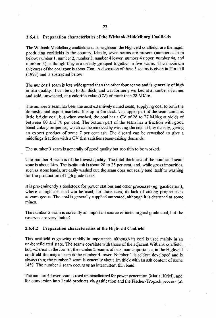
23

2.6.4.1 Preparation characteristics of the Witbank-Middelburg Coalfields

The Witbank-Middelburg coalfield and its neighbour, the Highveld coalfield, are the major producing coalfields in the country. Ideally, seven seams are present (numbered from below: number 1, number 2, number 3, number 4lower, number 4 upper, number 4a, and number 5), although they are usually grouped together in five seams. The maximum thickness of the coal zone is about 70m. A discussion of these 5 seams is given in Horsfall (1993) and is abstracted below:

The number 1 seam is less widespread than the other four seams and is generally of high in situ quality. It can be up to 3m thick, and was formerly worked at a number of mines and sold, unwashed, at a calorific value (CV) of more than 28 MJ/k:g.

The number 2 seam has been the most extensively mined. seam, supplying coal to both the domestic and export markets. It is up to 6m thick. The upper part of the seam contains little bright coal, but when washed, the coal has a CV of 26 to 27 MJ/kg at yields of between 60 and 70 per cent. The bottom part of the seam has a fraction with good blend-coking properties, which can be removed by washing the coal at low density, giving an export product of some 7 per cent ash. The discard can be rewashed to give a middlings fraction with a CV that satisfies steam-raising demands.

The number 3 seam is generally of good quality but too thin to be worked.

The number 4 seam is ofthe lowest quality. The total thickness of the number 4 seam zone is about 14m. The in-situ ash is about 20 to 25 per cent, and, while gross impurities, such as stone bands, are easily washed out, the seam does not really lend itself to washing for the production of high grade coals.

It is pre-eminently a feedstock for power stations and other processes ( eg. gasification), where a high ash coal can be used; for these uses, its lack of coking properties is advantageous. The coal is generally supplied untreated, although it is destoned at some mmes.

The number 5 seam is currently an important source of metallurgical grade coal, but the reserves are very limited.

2.6.4.2 Preparation characteristics of the Highveld Coalfield

This coalfield is growing rapidly in importance, although its coal is used mainly in an un-beneficiated state. The seams correlate with those of the adjacent Witbank coalfield, but, whereas in the former, the number 2 seam is of maximum importance, in the Highveld coalfield the major seam is the number 4 lower. Number 1 is seldom developed and is always thin; the number 2 seam is generally about 1m thick with an ash content of some 14%. The number 3 seam occurs as an intermittent thin band.

The number 4 lower seam is used un-beneficiated for power generation (Matla, Kriel), and for conversion into liquid products via gasification and the Fischer-Tropsch process (at

24

Sasol 2 and 3). The seam has a mean thickness of just under 4m, with a raw CV of from 18 to 25 MJ/kg. In some areas, the number 4 seam contains a high grade: fraction (more than 27 MJ/kg) that can be washed out, and the field may therefore be the scene of major preparation developments in the future (Horsfall, 1982).

The number 5 seam seldom exceeds 2 m in thickness and can be less than 1 m thick. It consists mainly ofbright coal sometimes with duller coal towards the top. It is restricted to the higher ground and can be mined where it occurs largely for blend-coking coal. In the outlying areas of the coalfield the rank ofthe coal is lower, with consequent loss of coking properties.

2.6.4.3 Characteristics of Highveld fine coal

There is currently no published information with respect to the characteristics of fine coal from the Highveld number 3+4 seams. It is thus an objective of this study to fully characterise Twistdraai fine coal (Highveld seam 3+4) using the methods described in section 2.2 of this thesis, prior to developing a fine coal circuit for the colliery.

2. 7 FINE COAL BENEFICIATION

Coal beneficiation plants have been in existence for over 100 years. Their purpose is to take the run of mine coal (RO.M) and tum it into a sized and consistent product suitable for the market. The operations carried out are the reduction of ash content, the removal of mining wastes, and the regulation of size. This processing can be divided into 5 levels, ranging from simply crushing the RO.M coal to a particular topsize for use in power generation and oil-from-coal plants (level 1 ), to re-crushing the coarse product with another stage offines beneficiation (level 5) (Horsfall, 1993).

Coarse (+ 15mm) and small (-15+0.5mm) coal is generally beneficiated using gravity separation units. The coarse coal is treated in either dense medium baths or jigs, with the general trend in South Africa being towards baths. The small coal is generally treated in centrifugal units, eg. cyclones or dynawhirlpool washers.

Processes developed to beneficiate fine (-0.5+0.1mm) and ultra-fine (-0.1mm) coal rely on differences in relative density or surface activities of the particles to be separated. Because separations are made on a particle by particle basis, there are many more accept/reject decisions made in treating fine coal than in treating the same mass of coarse or small coal.

Also, as each separator requires a certain amount of time to make the accept/reject decision, fine coal cleaning devices either have a lower capacity or make poorer separations (usually both} than units treating coarse or small coal. Consequently, fine and ultra-fine coal cleaning units need to be larger or more numerous than coarse or small coal units treating the same quantity of fine coal. This results in more plant floor space and higher unit capital and operating costs per ton treated (Osborne, 1988).

25

This section of the review is aimed at identifYing the separation technologies available for the treatment of fine and ultra-fine coal. Both gravity concentration and surface based separation methods will be generally discussed with respect to: principle of separation, range of application, extent of use, efficiency of separation etc. This is followed by a detailed discussion of the equipment selected with respect to this project.

2.7.1 GRAVITY CONCENTRATION METHODS

The term "gravity concentration" is usually applied to processes in which particles are separated from one another by employing their different settling rates in water. It is also, rather confusingly, use~ to describe processes in which the separation is carried out in fluids other than water, eg. in dense media such as a suspension of magnetite or shale. However, the classical theory of particle separation by differential settling velocity is properly applied only to motion in a fluid, such as water, in which all the particles involved sink. An explanation of settling theory application to practical settling conditions can be found inHorsfall (1993).

Gravity methods of separation are used to treat a great variety of minerals ranging from galena (R.D. 7.25) to coal (R.D. 1.45). Gravity concentration is useful down to 74 Jlm although special concentrators are capable of treating fines down to 15 Jlm, but feed tonnage is very low.

Gravity concentration methods separate minerals of different density by their relative movement in response to the forces of gravity and one or more other forces. The latter being the resistance to motion, often by a viscous fluid (water or air).

It is essential for effective separation that a marked density difference between the economic mineral and' the gangue should exist. Some idea of the type of separation possible can be gained from the concentration criteria:

Where Dh is the relative (RD) density ofthe heavy mineral. Dr is the relative density of the fluid medium. D1 is the relative density of the light mineral.

(3)

Generally, providing the feed material does not contain many ultra-fines, when the quotient is greater than 2.5, gravity separation is relatively easy. At 1. 75 RD., commercial separation is possible down to 150 Jlm. At 1.5 RD., the lower size limit is 1.5 mm and at 1.25 R.D., gravity concentration is not possible.

The motion of a particle in a fluid is dependent not only on its density, but also on its size. Efficiency of gravity processes decrease with particle size, i.e. movement of particles less than 74 11m are dominated by surface friction and respond poorly to gravity concentration. In commercial gravity concentration, efficiency of separation is always improved if the feed is either classified or sized.

26

Fine coal gravity concentrators include jigs, tables, spirals, water-only and dense medium · cyclones, upward current classifiers, and enhanced gravity concentrators. These will be briefly discussed in this section of the review.

2.7.1.1 Concentrating table

The concentrating, or shaking table, a form of flowing film separator, is one of the oldest and most widely used small and fine coal cleaning devices. It consists of a large flat rectangular surface, almost horizontal in shape, covered by a series of paraiiel ridges known as riftles. The table is slightly tilted in both directions away from the feed. Water, known as dressing water is introduced all along the upper edge, discharging along the lower, clean coal side. Feed coal is introduced along the same edge, at the highest point. The most commonly used type of table is the Deister table: There are probably of the order of3 000 in operation in the U.S.A. Tables are also fairly widely used in Australia. They were used successfully in South Africa to re-treat flotation plant tailings, but have been superceeded by spirals (Franzidis, 1995). A schematic of a Deister "88" double-deck table is given in Figure 2.5.

0.

oo

co . . . ()

. ·.~- :· .· .... . .

•• ()

DRESSING WATER

• • •

• COAL .

() MIDDLING

Q REFUSE

·Figure 2.5 Schematic of a Deister "88" double-deck coal washing table

The deck moves horizontally, at right angles to the flowing film, with a rapid movement from right to left, and a slow return from left to right. This results in a separation of the feed solids by size, relative density, and, to a lesser extent, by shape. Riffles increase the capacity of the table, and provide troughs in which hindered settling 6c:curs. Particles having a higher density, because of stratification behind the riffles, and th1~ asymmetrical acceleration of the deck, travel towards the end.

27

Tables are produced in standard sizes; their capacity determined by the feed rate possible at a given size of feed. Generally, the standard table is rated at 1 Otph for <8mm coal, and· 7. 5tph for <3 .2mm feeds. The table is little used to treat fines alone; the fines cleaning effect obtained results from feeding <12mm to a table.

Tables are oflow cost, low maintenance, flexible, easy to control, and require minimal water. They can be used on all ranks of coal sized below about 1 Omm, and are particularly · efficient in removing flat particles (which tend to be shaley) and pyrite. Tables are however not tolerant of coals ofvarying washability, or have >10% near-density, or have a high discards content. The commonest causes of poor efficiency are over-feeding, variations in size consist, and poor adjustment of the dressing water.

Separation is characterised by an increase in the cut-point d50 and ecart probable ( epm) with decrease in particle size as shown by the data in Table 2.3 quoted by Luckie (1987).

TABLE2.3 SEPARATION CUT-POINT AND EFFICIENCY DATA AS A FUNCTION OF PARTICLE SIZE FOR A DEISTER TABLE (AFTER LUCKIE, 1987)

PARTICLE SIZE FRACTION (mm) dso Epm

9.50 X 6.35 1.50 0.06 6.35 X 2.40 1.51 0.07 2.40 X 1.20 1.215 0.08 1.20 X 0.60 1.54 0.105 0.60 X 0.30 1.58 0.14 0.30 X 0.15 1.71 0.17 0.15 X 0.075 1.88 0.36

2.7.1.2 Water-only cyclone (autogenous cyclone)

The water-only cyclone (WOe) is a member of the hydrocyclone family, with an upper cylindrical section and a lower conical section. In contrast to the classifYing cyclone and the dense medium cyclone, the woe has a short, wide-angled cone (up to 120° vs 20°) and a long vortex finder. A schematic of a WOe is given in Figure 2.6.

...... PreSsurized Slurry enters tangentially

Light particles move inward and upward as IIPiraiHng vortex

28

Overflow discharge

Slurry rotation develops high centrifugal forces throughout cyclone

___.,;. Heavy particles driven ~-·-..1 toward wall and downward

in accelerating spiral

Underflow discharge

Figure 2.6 Schematic of a typical water-only .cyclone (Autogenous cyclone)

It is interesting to consider the effect of the changes in cyclone dimensions. Increasing the size of either ofthe exit openings ofthe cyclone increases the flow through it. Increasing the diameter of the vortex finder increases the yield and ash content of th(~ washed coal, and the relative density of separation ( d50), whereas, increasing the diameter of the underflow opening decreases the yield and the ash content of the washed coal. Increasing the length of the vortex finder increases the probability of a light particle leaving through the overflow and therefore increases the d50, the yield and the ash content of the washed coal.

The WOe is generally only effective on -K>.15mm coal; the ·0.15mm coal UISUalJy reports to overflow essentially uncleaned, and needs to be removed from the clean coal, for example using a sieve bend. In general, the WOe exhibits increasing relative density of separation with decreasing particle size, which is also accompanied by a decrease in efficiency, as shown by the data in Table 2.4 quoted from Hornsby et al (1983).

TABLE 2.4 SEPARATION CUT-POINT AND EFFICIENCY DATA AS A FUNCTION OF PARTICLE SIZE FOR THE WATER-ONLY CYCLONE AFTER HORNSBY et al (1983)

PARTICLE SIZE FRACTION (mm) dso Epm

0.50 X 0.25 1.55 0.11 0.25 X 0.125 1.90 0.22

0.125 X 0.075 2.35 0.33

29

The WOC can be used for all ranks of coal and has the advantage ofbasic simplicity, high capacity and low capital cost. However, water and power requirements are relatively high, and some degree of operator skill and experience is needed. WOC's are used widely in North America to process high sulphur raw coal because of the efficient pyrite rejection. In Canada especially, there is a heavy reliance on WOC's: in 1985, the WOC accounted for approximately 21% of all coal washed in Canada (Franzidis, 1995).

The capacity of a 200mm diameter WOC is 5tph, increasing to 15 tph for a 300 mm unit. Generally, two-stage operation is required to achieve high quality ofboth clean coal and discard. They are being used more often in new preparation plants as rougher separating devices that decrease the load on downstream cleaning equipment (Franzidis, 1995).

2.7.1.3 The dense medium cyclone

Suspensions of finely-divided solids in water can closely approach the properties of heavy liquids in sink and float processes. If the solid phase of the suspension is ground to a suitable degree of fineness, and mixed with water in the correct proportion, a medium is obtained that is stable, or so slow settling, that a substantially uniform pulp density can be maintained from top to bottom of the bath containing such a liquid. As a consequence, no rising currents ofwater are necessary to assist in the separation of minerals that will either float or sink.

Dense medium cyclones are in widespread use for the beneficiation of small co a! ( 15 n1m x 0.5 mm). The same kind ofunit can be employed for the treatment of fine coal, but the diameter is smaller (150 mm), and a finer medium is required (micronised magnetite). A lower feed slurry concentration must also be used, as well as a higher cyclone inlet operating pressure.

As far back as 1949, VanDer Walt indicated that sharp separations of -0.5mm material could be affected in a dense medium cyclone. At the same time however, it was appreciated that the medium recovery problem would be formidable and this avenue was not pursued.

In 1957, the Dutch State Mines designed and built two dense medium cyclone plants in Belgium which treated 10 x Omm feed with effective cleaning to about 150J..lm. Similar plants followed in the U.S.A. but although encouraging, the separations were not of the required sharpness (Franzidis, 1995).

Deurbrouck ( 197 4) showed the suitability of dense medium cyclones for washing down to 75 J..lm. Sokaski and Geer (1975) made similar reports and produced several papers on the subject.

In 1977, it was reported by Fourie and Erasmus that the conventional fine coal treatment processes such as froth flotation, tables and water-only cyclones were all tested by the Fuel Research Institute with negligible success, indicating, once again, that South Mrican coals would require a special approach.

30

The data obtained from the work ofFourie and Erasmus (1977), was used in designing the first commercial-scale plant to be built in South Mrica. This was completed in 1980 at Greenside colliery. It treats 0.5mm x 0.075mm coal at a feed rate of 45tph, and no operating data on the plant is currently available. There are 4 plants operating worldwide: Homer city in the U.S.A.; Greenside in South Africa (intermittent); and two plants in Australia. The following efficiency data have been reported from the Homer city coal cleaning plant (Chedgy et al, 1986) and is given in Table 2.5.

TABLE 2.5 SEPARATION CUT-POINT AND EFFICIENCY DATA AS A FUNCTION OF PARTICLE SIZE FOR FINE COAL, DENSE MEDIUM CYCLONES OPERATING AT THE HOMER CITY PLANT, AFTER CHEDGY et al (1986).

PARTICLE SIZE FRACTION (mm) dso Epm

3.00 X 1.00 1.31 0.02 1.00 X 0.50 1.38 0.03 0.50 X 0.15 1.43 0.06

As suggested by Vander Walt in 1949, the main problem with this technology has been unacceptably high medium losses; and not-separator efficiency.

2.7.1.4 Fine coal Feldspar jig

Jigs are used extensively to clean coal. They are of high capacity, low cost, but generally of low efficiency. In a jig, water is cycled up and down through a bed of raw coal retained on a screen. For coarse coal the Baumjig operates by means of a plunger, while in the fine coal feldspar jig use is made of air pressure. A schematic of a fine coal jig with superimposed air cycle is given in Figure 2. 7.

On the upward (pulsation) stroke, the bed expands and lifts from the screen. Small light particles move rapidly upwards, while the larger-denser ones fall down through the bed under conditions ofhindered settling. Towards the end of the pulsation stroke, the upward velocity of the water decreases, so that heavy particles settle to the screen. On the downward (suction) stroke, the water flow changes direction, and all particles descend towards the screen, again with the heavier particles settling more rapidly than the lighter ones.

31

r1 = 15· 30/min ) Pii = 0.04- 0 .. 1 bar

Roloryoir valves Pulse height 35 mm

Figure 2. 7 Schematic of a fine coal jig with superimposed air cycle

In addition to the screen, the Feldspar jig uses a bed oflarge particles of feldspar, 50 to 70mm in diameter, which are too large to pass through the screen. This is to prevent fine clean coal particles passing through the screen apertures. On the pulsation stroke, the feldspar bed opens and allows small particles to fall through. On the downward stroke, the bed closes. The feldspar particles are retained on an iron grid which rests on the screenplate.

The feldspar jig is used extensively in Europe for cleaning - 12.5mm coaL Good separations are obtained on raw coals containing less than 15% near-density material (± 0.1 RD.). Very little reduction in ash is obtained in the -0.3mm size fraction, although desliming of the feed is not necessary (Franzidis, 1995).

Killmeyer (1980) quotes a capacity of 16 tph/m2 for a fine coal jig, and the following separation efficiencies by size fraction is shown in Table 2.6. ·

32

TABLE 2.6 SEPARATION CUT-POINT AND EFFICIENCY DATA AS A FUNCTION OF PARTICLE SIZE FOR THE FINE COAL FELDSPAR JIG AFTER KILLMEYER (1980)

PARTICLE SIZE FRACTION (mm) dso J~pm

12.70 X 6.35 1.50 0.09 6.35 X 2.40 1.55 0.11 2.40 X 1.20 1.70 0.14

. 1.20 X 0.60 1.90 0.19

2.7.1.5 Spiral concentrator

The spiral is another kind of flowing film concentrating device, in which a centrifugal force is superimposed on the flowing film by means of a multi-turn helical trough.

--Aefuse-collecflng pipe __..,.,......_ ___

Spiral section

Pump

Figure 2.8 Schematic of a typical spiral concentrator

Due to the combined action, the lower relative density particles migrate to the outer rim, while, the denser particles migrate to the inner edge. The exiting stream may be split into clean coal, middlings and discard. Reject splitters situated. along the length of the trough remove discard continually, via a pipe running into the centre of the spiral, or an inner gutter. A schematic of a spiral concentrator is given in Figure 2.8.

In general, spirals have a high relative density of separation ( d50), and an efficiency which is a function of particle size. Spirals are capable of producing excellent pyritic sulphur

..

. ,<;.·

33

reductions down to 0.075mm, but ash reduction is dependent on the proportion of near-density material. ·

Spirals exhibit increasing relative density of separation with decreasing particle size, while the efficiency is decreasing as shown by the data in Table 2. 7 quoted from Hornsby et al (1983).

TABLE 2.7 SEPARATION CUT-POINT AND EFFICIENCY DATA AS A FUNCTION OF PARTICLE SIZE FOR THE SPIRAL CON CENTRA TOR AFTER HORNSBY et al (1983)

PARTICLE SIZE FRACTION (mm) dso Epm

0.50 X 0.25 1.90 0.22

0.25 X 0.125 1.95 0.32

0.125 X 0.075 2.15 0.50

On account of their low capital and operating cost and maintenance-free operation, spirals have aroused much interest for fine coal cleaning in the last few years, all over the world. In South Africa alone at least 14 spiral plants are known to have been installed since 1984. Current interest is in the treatment of hitherto untreated l.Omm x 0.1mm fines, although in some cases, spirals have been retrofitted into plants to replace other, less successful units (Horsfall, 1993).

2. 7.1.6 Upward current washer or hindered-bed classifier

The upward current washer or hindered-bed classifier is simply a cylindrical vessel into which the feed is added centrally, via a curtain wall. Low density material rises and overflows all round the cylinder, higher density particles are withdrawn from the bottom.

Now, where materials oftwo specific gravities are to be treated (e.g. coal/shale mixture), the material with the greater mass will create a teeter (suspended bed) column in the upward current classifier. The coarser, heavier material will penetrate the zone of teeter, i.e. particles containing mostly rock, which have a settling velocity nearly equal to the teeter water velocity become suspended, thereby creating a fluidised hindered settling bed. The lighter mass material (plus the fine heavier material) will be buoyed into the overflow. A schematic of a typical upward current washer is given in Figure 2.9.

Recent studies have found that hindered-bed classifiers can provide an efficient and cost effective alternative to technologies such as spirals and water-only cyclones, for the treatment of -1.2 mm x 150J.lm fine coal having easy-to-clean characteristics (Mankosa et al, 1995; Reed et al, 1995).

Product Overflow

Hindered· . Settling . (teetering) Bed

Tailings Thickening

Figure 2.9

34

Product (coarse coal, fine 1::oal, fine rock)

DJ • •• Bed Level Controller

.;.--Water Addition

High Ash Content Tailings .

Schematic of a typical upward current washer

The unit requires a high pulp density, and if the fine material forms viscous slimes it cannot operate efficiently, if at all. However, it may find an application in South Africa where the fine discard tends to be less slime-forming. The separator is really a size classifier, and is also so used; it is only under high pulp density conditions that it also acts as a density separator (Horsfall; 1983).

In a study by Honaker et al (1995), it was found that the Floatex upward current washer was found to be superior to spirals for the treatment of an Illinois no 5 seam coal when treating -1.2 mm coal. This superiority was found mainly in the ;..1.2 mrn + 150 ~m size fraction, in terms of both ash and sulphur rejection at a given recovery. This superior performance was further observed by the relatively low probable error value of 0.12 achieved by the Floatex compared to a value of0.18 obtained by spirals.

Subsequently, Honaker (1996) investigated two pilot-scale hindered-bed classifiers i.e. Floatex and Stokes in an in-plant test programme at the Kerr-McGee Galatia plant in Marion illinois. It was reported that both upward current washers reduced the ash content of a nominally -1.2 mm x 150 ~m Illinois no 5 coal sample from about 30% to 9%, while recovering greater than 90% of the combustibles. This separation performance was consistently achieved over a 16 hour long in-plant testing programme.

Honaker (1996) further concludes the following operational and design advantages of using the upward current washer over currently used technologies such as spirals: a lower floor ~pace requirement to treat a given capacity, a high density tailings stream ( c.a. 70% by weight), elimination of a feed distribution and product collection system, reduced

35

plugging in the system caused by excessively large particles, and an improved ability to adjust to changing feed characteristics.

The following efficiency data for the stokes upward current washer has been published by Hyde et al, (1988) and is given in Table 2.8.

TABLE 2.8 STOKES UPWARD CURRENT WASHER EFFICIENCY DATA (AFTER HYDE et al, 1988)

SIZE FRACTION

EFFICIENCY FACTOR +lmm -1mm+0.5mm -0.5mm + 0.25 mm

Separating density 1.38 1.53 1.89

Probable error (epm) 0.038 0.063 0.195

Imperfection (I) 0.100 0.119 0.219

Organic efficiency 86.9 98.4 94.0

Over 40 upward current washer units are currently operating commercially (2m diameter machine can treat upto 150tph of feed) on northern hemisphere fine coal circuits, and pilot-scale testwork in Australia is at an advanced stage (Hyde 1996).

2. 7 .1. 7 Enhanced gravity concentrators

Several new gravity devices (non dense media methods) are now in various stages of development and testing for coal use. These devices attempt to enhance particle inertia relative to surface drag forces by application of a centrifugal field. Several of these devices are: the Kelsey centrifugal jig, the Falcon concentrator, and the Knelson concentrator. Another device called the Mozley multigravity separator uses the flowing film technique for coal- ash separation. Luttrell, et al (1990) report that by using the Mozley device, rejection of fine pyrite is possible, and that performance is improved if the high levels of ash material are removed (by froth flotation) prior to gravity cleaning. The raw coal used in these tests was 80% -0.075mm. Because ofthe inherent limitations of flowing film devices, large multi-ton units necessary for today's modern coal cleaning sites will not be forthcoming. Thus the cost for cleaning coal will be too high for commercial use (too many units required) (Fonseca, 1996).

2.7.1.8 Summary of fine coal gravity concentrators

Separation cut-point and efficiency data as a function of particle size for the fine coal gravity devices reviewed is summarised in Table 2.9.

36

TABLE 2.9 SEPARATION CUT-POINT AND EFFICIENCY DATA AS A FUNCTION OF PARTICLE SIZE FOR THE FINE COAL GRAVITY DEVICES REVIEWED

DEVICE SIZE (mm) CUT POINT Epm (dso)

Concentrating table 0.6-0.3 1.58 0.14 Water-only cyclone 0.5-0.25 1.55 0.11 Dense-Medium cyclone 0.5-0.15 1.43 0.06 Feldspar jig 1.2-0.6 1.90 0.19 Spiral concentrator 0.5-0.25 1.90 0.22 Stokes upward-:-current washer 0.5-0.25 1.89 0.195

From the data in Table 2.9, as well as the data in section 2. 7.1 it can be observed that: the dense-medium cyclone clearly yields the sharpest separation i.e. a cut point of 1.43 and epm of0.06 when treating particles in the size range 0.5mm x 0.15mm. However; the fact

· that only 4 fine coal dense-medium· circuits are currently operating worldwide, and the intermittent operation of the Greenside plant treating high grade Witbank coal, all appear to indicate that the process is a difficult one to operate technically. Furth~;:rmore, high medium losses represent a decrease in process economics. Also, given the tight time constraint in developing a fine coal circuit for the Twistdraai colliery, wherein a "simple" but functional process ·scheme is required, the option of dense-medium cyclones unfortunately has to be excluded here.

Of the non-dense media devices, the water-only cyclone appears to be the most efficient when treating particles 0.5mm x 0.25mm. These devices are used extensively on northern hemisphere coals, but are not favoured in South Africa since they only tend to reduce the ash content by c.a. 5% (Horsfall, 1993); and multiple stages of water-only cycllones would be required to reduce the ash content of the Twistdraai fine coal to below 10% ash.

Concentrating tables are quite efficient, low capacity units (7.5tph <3.2mm coal). They are extensively used to treat northern hemisphere coal, but are currently not used in the South African coal industry. They were used successfully in South Africa. to re-treat flotation plant tailings, but have been superceeded by spirals.

Although first introduced over a century ago, the jig remains well established as the most popular coal washing unit, on a worldwide basis. It's simplicity, both as a unit and in

·terms of the water circuit required, ability to deal with a wide size range, and non-use of medium or reagents, make it prime choice if the coal to be washed has the right characteristics. However such coals, with near-density percentages under 10% and even under 5% are uncommon in South Africa.

The jig concentrator, like the water-only cyclone and concentrating table are not used in the South African coal industry. These units are reasonably inefficient i.e. cut point of 1.9 and epm of0.19 on 1.2n1m x 0.6mm coal.

37

The spiral concentrator has dominated the fine coal preparation scene in South Mrica over the last decade, treating c. a .. 11. 5mt of coal annually. These simple to operate, cheap devices, have yielded increased efficiency with the introduction of the LD (large diameter) spirals.

The Stokes upward current washer is also a simple low-cost unit which offers the advantages of controllable variable cut-points in the range 1.38 to 1.90 with epm's between 0.038 at +1mm, and 0.195 at -0.5+0.25mm. The low cost ofthe unit arises largely from the high capacity of the units, eg. a 2m diameter unit may treat as much as 150tph of feed. The operation of the unit is insensitive to feed rate variability and has been successfully demonstrated at several Australian mines. This device appeared to. be an . option worth considering for the Twistdraai plant.

2.7.2 Gravity equipment selected for this project

From the above discussion, the spiral concentrator and the Stokes upward current Washer were chosen as fine coal beneficiation technologies worth investigating for the Twistdraai Colliery. These devices are both discussed now in more detail below.

2.7.2.1 The spiral concentrator

2.7.2.1.1 Operating characteristics of spirals

The operating characteristics ofthe South African spiral plants surveyed in 1990 and 1995 are given in table 2.10 (after Harris and Franzidis, 1995).

It can be seen that the most dramatic change has been with respect to the type of spiral employed. In 1990, nearly all the plants were using "standard" coal spirals with a nominal diameter of about 750mm, with 2 manufacturers, Multo tech and Mineral Deposits, equally represented. A number of problems were reported by the users of these spirals, mainly . with respect to "beaching", pyrite blockages, and capacity limitations. By 1995, most of the plants had changed to the new high capacity LD (large diameter) spirals. (Multotech: 1 OOOmm diameter; MDL: 966mm diameter), with Multotech clearly established as the primary supplier. The Multotech LD spiral can handle more than 3tph of solids per start, in comparison to 1.5tph for the standard unit, and the problems associated with the smaller diameter unit appear to have been eliminated (Harris and Franzidis, 1995).

From the data in table 2.1 0, Harris and Franzidis (1995) also indicate that a 1:1 split with respect to single and two stage spiral circuit operation is observed in 1990, and in 1995, single circuit operation is clearly favoured. This can probably be ascribed to the fact that on a number of plants, two stage circuits were installed with the aim of producing two products, a high grade coal for addition to the "low ash" product, and an export grade thermal coal. In practice, it has not proved possible to upgrade the fines sufficiently for addition to the "low ash" fraction, even using two stages of spiral washing, while a satisfactory export grade thermal coal can· generally be achieved with relative ease in a single stage. The majority of plants are now operating at between 30-35% solids without problems.

38

TABLE 2.10 THE OPERATING CHARACTERISTICS OF SPIRAL PLANTS IN SOUTH AFRICA, 1990 AND 1995 (AFTER HARRIS AND FRANZIDIS, 1995)

1990 1995

Equipment: Multotech (standard) 8 6 Multotech (LD) 1 9 Mineral Deposits (standard) 8 4 Mineral Deposits (LD) I 3

Circuit: Single Stage 8 13 Two Stage 8 9

Plant Capacity (tph) 5-260 19-500

Throughout (% of total feed) 4-20 6-20

Feed Pulp Density (mass%) 15-30 . 20-36

Feed Source: Current fines 13 21 Retreat discards with current fines 2 ' 1

Retreat discards only 1 -Product: Export Steam Coal 10 17 ISCOR (coking coal) 4 3 LOCAL/ESKOM 3 7

·Performance: Feed ash content(%) 17-46 14-55 Product yield (%) 30-86 :25-90 Product ash content (%) 10-19 12-50 Discard ash content (%) na 30-67

Dewatering: Centrifuge(+/- screen & cyclone) na 14 Belt· filter na 3 Dewatering screen only na 3

2.7.2.1.2 Spiral operating parameters

The feed parameters that can affect spiral operation are summarised in table 2.11 (after Mikhail et.al., 1987).

. _,.,,(,"

39

TABLE 2.11 SUMMARY OF FEED PARAMETERS THAT CAN AFFECT THE SPJRAL SEPARATION

Parameter Operating conditions

Feed rate -- 1-3 tph (dry solids) -- high feed rate causes low separation efficiency

and high cutpoint

%Solids -- limit influence on separation -- usually 20-40 % (by mass) -- high feed ash requires lower % solids

Particle size -- top size 3mm, but 1 mm is preferable -- 0.075 mm is the effective bottom limit -- desliming is recommended

Spiral variables are pitch, profile, radius and number of turns, or length. The pitch affects the velocity of the descending pulp, which directly impacts upon the hydro- dynamics of the operation. In general, the greater the density difference between the product and the discard, the greater the pitch. Fine particles require a more horizontal pitch. The optimum profile is generally determined by trial and error, with some assistance by theory. Smoothness of the surface is very important. Although it is stated (Horsfall, 1993) that the radius simply determines the capacity of the unit, the success of the (LD) spirals compared to the standard diameter seem to contradict this comment. Length relates to the time required to effect a separation; extra length has no particular benefit. ·

Spirals are low-capacity units, so it is common to find two or more "starts" per unit, i.e. the units are orientated one within the other to occupy the same space. They are now being made cheaply from lightweight polyurethane coated fibreglass. The common upper limit of feed size is 3mm, and the lower limit about 0.075mm. Spiral capacity is 2 to 3 tph dry solids per start, depending on the trough diameter and the discard content. Feed rate is in fact the most important parameter governing spiral performance. Pulp densities of 20 to 40% by mass of solids in the feed and 30 to 60% in the discards are normal. The increasing use of spirals has led to developments in trough profiles, splitter design, and in some cases, the elimination of the need for wash water (Horsfall, 1993).

Goodman et.al. (1985) report that spirals tend to separate on the basis of particle mass rather than density, and thus are best applied to treatment of relatively narrow size ranges. They concluded that in some cases, it may be necessary for spirals to be used in conjunction with other cleaning processes eg. froth flotation, rather than replacing them to achieve optimum separation. Spirals application for a particular coal should be tested before hand, since, in some cases, other processes such as froth flotation may be able to achieve equivalent, and sometimes superior performance compared to that of a spirals circuit. (Bensley and Keast-Jones, 1985).

40

2.7.2.2 Stokes upward current washer

2. 7.2.2.1 Theoretical basis of density separation

The theoretical basis for the density s~paration achieved in the upward current washer is shown in Figure 2.10, after Honaker, (1996). The plot shows the theoretical settling velocities of spherical particles of pure coal, rock and pyrite particles having specific gravity values of 1.3; 2. 7; and 4.5 respectively. The calculations were performed over a particle size range ofO to 3 mm using the well known Stokes and Newton free-settling equations, and the Ergun and Concha hindered-settling equations.

1E+2~------------------~-----------

lE+l

lE+O ----... -.... - - -

... ·. ------------___ ...

>. ~ lE-1

- Sp. Gr.: 1.3 Sp. Gr.= 2.7 Sp. Gr.= 4.5

u 0

~ = ·­-.._ -c:; en

lE-4 i

\ i l Settling Ratio = 2 - 3:1

lE-5 ~~._. '---~-----l----------'----0 0.5~ 1.5 2 2.5

Particle Size (mm)

Figure 2.10 Theoretical basis for the density separation achieved in the upward current washer (after Honaker, 1996)

According to the theoretical calculations in Figure 2.10 an upward current 'Yasher treating a -lmm feed coal would achieve efficient separation between coal and rock within the size range of0.4 to l.Omm and 0.3 to 1.0mm for coal pyrite, which is equivalent to a particle size ratio of about 2 - 3: 1.

2.7.2.2.2 Design criteria- Stokes variables

In commercial practice, units operating on teeter (suspended bed) principle allow the pulp density to build up within the separating vessel, against an upward current ofliquid, until a bed is formed in which the average particle suspension is such ·that a "perfect" suspension is formed. In such a bed, the particles tend· not to separate. In chemical

41

engineering parlance, the bed is described as levitated or fluidised, and the value of the liquid velocity at which this occurs is the incipient fluidisation velocity. Under these conditions, the solids are said to be in condition of full teeter, and hence the name teetered bed separator {TBS).

Over the years there have been numerous pieces of equipment developed which fall into this category including:

- The Richards-Janney separator - The Fahrenwald sizer - The Bunker Hill classifier - The Pellet classifier - The T -type classifier - The Conenco classifier - The Stokes hydrosizer

(Wills, 1981)

Basically, the various machines fall into two groups. In the earlier units, a conical · separating chamber was employed, but these met with operational problems arising from:

Non-uniformity of upward teeter water distribution arising from their conical shape. This results in cyclic banking of material against the sides of the unit, thereby reducing capacity and causing blockages.

Sanding of the units below the teeter distributor on start-up after shutdowns.

Local velocity gradients leading to density variations and hence poor efficiency (high Epm's).

As a consequence of the above factors, modern equipment developers have opted for the use of various forms of distributor plate located as low in the teeter chamber as is possible. From this background, the Stokes hydrosizer was developed (Hyde et al, 1988).

2. 7 .2.2.2.1 Shale cut size

The area of the teeter chamber sets the overall size of the upward current washer, and is calculated by selecting a "cut size" for the shale particles alone. Shale particles finer than this -size will report to the clean coal product. This selected "cut size" of shaJe is determined by the largest size of coal required to be displaced to the overflow. The cut size is typically 114 to 1/6 of the size ofthe coarsest coal (Hyde et al, 1988).

2. 7.2.2.2.2 Let-down rate

The shale let-down rate is defined as the capacity of the teeter bed to allow the passage of settling shale particles coarser than the cut size. This is expressed in terms of mass throughput per unit area (t/h/m2

). Clearly for a given duty, the settling rate of shale determines the minimum area of the vessel (Hyde et al, 1988).

42

2. 7.2.2.2.3 Upward-current water

Having fixed shale cut size and vessel area, the upward current water can be calculated. The settling velocity of any particle in the Stokes flow regime is inversely proportional to the viscosity of the fluid through which it is falling. For this reason it is not usually possible to use dirty water to supply the upward current water to the washer. Clearly, as the viscosity of such circulating streams is increased by their suspended solids content, the velocity of the upward current water must be proportionally decreased. This would result in an effective increase in the separation density of the Stokes washer, and a poorer quality product. Therefore it is recommended that clarified water is used for upward. current teetering (Hyde et al, 1988).

2.7.2.2.3 Pilot unit operating data

Hyde et al, (1988) reports that a Stokes pilot unit used for feasibility studies (0.6m in diameter), has an estimated capacity of 4tph. For this device, teeter water should be supplied at a rate of approximately ll/s from a water head tank providing 7m of operating head. The raw feed coal slurry should ideally have a solids concentration in the range 40 to 60%. This machine will theoretically classify at any size within it's working range i.e. 5mm x 0 material.

In order for the unit to operate effectively, the average relative density of the teetered suspension within the vessel must be kept constant. To achieve this, a simple control system comprising a probe, bed density meter and PID controller unit is fitted. The teeter bed density is monitored by the probe immersed in the teeter zone. The controller compares the actual density from the bed density meter, to the required density (controller set point), and produces a compensation value~ This electronic signal is fed to an electro-hydraulic actuator, and causes the actuator to progressively open or close allowing the coarser or heavier minerals to pass through the spigot, and thus maintain the required teeter bed density.

2. 7.3 Separation based on the surface properties of coal

This section of the review begins with a brief general introduction to surface based separation methods for coal fines. This is followed by a detailed discussion on froth flotation which includes both coal floatability effects as well as froth flotation cells. This section is concluded by a detailed discussion of the equipment selected with respect to this thesis.

The cleaning methods so far described have all relied upon differences in n~lative density between the particles to affect separation. Below a certain particle size however, fineness becomes a complication, and the separation tends to be on the basis of size rather than density, i.e. the units function as classifiers. This limiting size varies from unit to unit, but a lower limit of about 0.15mm with those currently in use is generally accepted (HorsfalJ, 1993).

43

Particles smaller than 0.15 mm are better separated by methods relying on differences in surface activity, such as froth flotation, oil agglomeration and selective flocculation. These methods utilise the fact that coal, like oil, has surface properties that make it hydrophobic i.e. water repellent. This phenomenon is measured by the contact angle discussed in section 2.5.4.1 of this review. ·

According to Horsfall, (1993); selective flocculation has only been studied to a limited extent. He concluded that the problem with South Mrican coals are in the lack of selectivity, and that the difference in surface characteristics between a particle of 25% ash and one of30% ash is negligible, so that distinguishing between the two is almost certainly beyond the scope of selective flocculation.

Oil agglomeration on the other hand has been rather extensively investigated. The process consists of adding a reagent, usually an oil, to the pulp and agitating the mixture. It is found that the oil coats the coal, but not the stone. The oil-coated coal particles coalesce to form "caviar-like" balls of surprising mechanical strength which can be separated by screening from the pulp. The product drains well on a dewatering screen.

The results of a number oflaboratory studies have been reported (e.g. by Anglo American Corporation, Cape Town University and Potchefstroom University). The process can give high yields of low ash coal, the actual process of agglomerate formation probably restricting the degree of entrainment of non-coal particles. However, the process is costly in terms of oil consumption, and, more significantly, variable in performance.

Work at Potchefstroom University (Van Nierop et al, 1985) has shown the process to be highly sensitive to oxidation. In one series of tests, a change in the percentage COOH functional groups in coal from 0.8% to 1.8%, reduced the degree of agglomeration from 87% to zero. These COOH changes were brought about by heating the coal in air for various periods at various temperatures. Other workers in oil agglomeration, especially in the northern hemisphere, have indicated that the process is reasonably tolerant to coal changes. However, this might only be valid for their high vitrinite coals (Horsfall, 1993).

Froth flotation is widely used overseas to treat fine coal. It is in use in South Mrica in ~wazulu Natal and the Mpumalanga Province, but not extensively. Froth flotation is widely recognised as the most effective method to separate fine coal from minerals (Allum and Whelan, 1954), and for this reason, the selective flocculation and oil agglomeration technologies are dismissed in further discussion in this section.

In the frot_h flotation technique, a small quantity of reagents (fuel oil or kerosene and a frother, usually a low- carbon alcohol) are added to the coal slurry and mixed thoroughly. Air is then sparged into the slurry, and the hydrophobic coal attaches to the rising air bubbles. The mineral particles, being hydrophylic, stay in suspension (Wills, 1981).

Horsfall (1993), states that although froth flotation is not density-based, the surface activity is governed to a major extent by the mineral content. As the mineral content affects particle density, froth flotation efficiency can also be represented by the ecart probable (epm). It was further reported that an epm of>0.25 was obtained for coal finer

44

than O.Smm. No mention was made of the type of flotation device evaluated It is assumed, however, that this measurement was obtained using a mechanical froth flotation cell.

Horsfall (1986) points out that the essential problem with coal flotation is its lack of selectivity. A sample of coal (-500+150um) was separated firstly by float and sink analysis into a series of density fractions. These fractions were then floated under identical conditions and the results were almost independent of the ratio of coal to mineral matter. A further problem is that the density of coal is approximately 1.55 g/cm3

, which is much lower than for other minerals (eg. 2.7 g/cm3

). Thus coal solids occupy a greater percentage ofthe volume of a flotation unit than observed in any other mineral flotation process. The equipment used for froth flotation is generally the same as that used for mineral flotation. This is really an anomaly, as in most mineral separation processes, the froth yield is verylow (1-5%), whereas in coal it is very high (50- 90%).

2. 7 .3.1 Factors determining the floatability of coal

Froth flotation depends upon the differences between the physio-chemical surface properties of the coal and mineral fractions. Flotation occurs since the hydrophobic coal particle attaches to the air bubble (Wills, 1981 ). The mineral component is hydrophylic of nature, and remains behind in the tailings suspension. Three surface types can be differentiated, i.e.:

A hydrophobic surface which is naturally non-wettable in water. Polar hydrophylic surfaces.

. Surfaces which are heteropolar. Coal falls into this class since it has a hydrophobic carbon skeletal as well as hydrophylic surface functional groups (Hindmarch and Waters, 1951-52).

Various factors influence the natural hydrophobicity of coal, namely:

coal rank natural floatability functional group composition degree of oxidation slime-coating and entrainment particle size distribution flotation reagents petrographic composition ofthe coal pulp pH pulp density and temperature

(Leja, 1982; Van Nierop, 1986; Wheeler and Keys, 1986)

Further discussion is restricted to factors where the surface properties of coal play an important role.

45

2.7.3.1.1 Natural floatability

Although coal is generally hydrophobic in nature, the natural floatability in water varies with respect to origin and rank ofthe coal (Fuerstenau, 1982). Sub-bituminous coal is the most difficult to float whilst bituminous coal containing a low volatile content as well as semi-anthracite float easiest. This trend can be ascribed to the following factors:

The carbon content increases with an increase in rank. The oxygen content of coal decreases from 30% in lignite to 2% in high ranking coal (Wheeler and Keys, 1986).

2.7.3.1.2 Surface functional groups

The presence of oxygen-containing surface functional groups cause the adsorbsion of water molecules onto the coal surface. This negatively influences flotation since a hydrated layer forms on the coal surface (Bujnowska, 1985).

At typical coal flotation pH of between 6 and 8, coals invariably carry a negative surface charge (Fuerstenau, 1982). This surface charge arises largely from the presence of carboxylic (COOH) and phenolic (OH) functional groups, as well as mineral ions on the coal surface.

An increase in the surface fhnctional groups of coal occurs as the degree of oxidation increases leading to a decrease in floatability (Sun, 1954). The oxidation susceptibility of coal decreases with an increase in rank (Taylor et al., 1981).

2.7.3.1.3 Slime coating and entrainment

Slime is defined as ultrafine particulates which indefinitely remain in suspension. The presence of slime during flotation leads to excessive reagent usage, a decrease in recovery and an increase in frother requirement. Slime coatings can be ascribed to the electrostatic attraction between particles of opposite charge. The clay surface has a dual electrical charge which makes it easily bound to the negatively charged coal surface.

In order to minimise slime coating, Jowett et al., (1956) adsorbed negative ions onto the clay surface in order to create an electrostatic repulsion force between the clay and coal. surfaces.

Entrainment occurs when fine hydrophylic minerals are transported to the froth/water interface without being attached or bound to air bubbles.

2. 7 .3.1.4 Particle size distribution

Sun and Zimmerman (1950) report that coarser particle sizes often require more than one air bubble in order to float. The low floatability of these particles can also be ascribed to cell turbulence effects.

46

According to Wheeler and Keys (1986), the floatable particle size limits must be considered as a function of coal rank and hydrophobicity. eg. coarse coal particles of a low ranking coal are more difficult to float than for a higher ranking coal.

2. 7.3.1.5 Petrographic components

The floatability of coals increase with rank since high rank coals contain less oxygen than low rank coals (Y e et al, 1989). Similarly, coals rich in vitrinite can be 1expected to be intrinsically more floatable than coals containing predominantly inertinite. Bujnowska (1985) reports that the reactive coal macerals do not necessarily float first, claiming that the froth initially only contained vitrinite and inertianite. It was found that the inertianite concentration decreased steadily as the exinite concentration increased. Inertianite recovery was found to be highest, followed by vitrinite and exinite.

2.7.3.1.6 Frother dosage

The main purpose of frother addition during froth flotation is to increase the kinetics of the particle/bubble adhesion process (Leja, 1982). Frothers are generally heteropolar reagents (Brown, 1962) eg. short-chain alcohols such as methyl-iso-butyl-carbinol (mibc). Crecylic acid, pine oil and inorganic salts have also been used as frothers (Aplan, 1976). A frother must conform to the following requirements:

The stability of the froth formed must be of such a nature that a separation between floatable and non-floatable material is possible. When the froth is removed, the froth must break allowing recovered particles to be collected. Low concentrations of frother must provide a stable froth. The frother should have limited collecting properties since a collector is used for the purpose of imparting surface hydrophobicity.

2.7.3.1.7 Collector dosage

According to Fuerstenau and Pradip {1982), collectors are classed as either cationic, anionic and non"'ionic. Non-ionic collectors do not impart new surface hydrojphobicity, but only increase the surface hydrophobicity of existing hydrophobic surfaces (Nimerick and Scott, 1980).

Although flotation is mainly dependent on the rank and oxidation state: of the coal, floatability improves as a result of collector addition (Aplan, 1987).

Uniform distribution of collector over the coal Surface is a pre-requisite: for efficient performance. Collectors form strong bonds with hydrophobic high-ranking coals as well as un-oxidised vitrinite. For the more polar low-ranking coals, additional reagent is required in order to increase the hydrophobicity prior to effective collector bonding (Brown, 1962).

47

According to Aplan (1976), the amount of collector required for flotation is inversely proportional to the rank of the coal.

2. 7.3.1.8 Temperature effects

Aplan (1976) states that over a range of3-50°C, temperature has no significant effect on the rate of coal flotation.

2. 7.3.1.9 Coal pulp conditioning

Conditioning of coals using oily collectors is also strongly dependent on coal surface properties. From a thermodynamic viewpoint, the spreading of an oil film on a coal surface requires an energy input, termed the work of spreading, y •. Oils spread more easily (i.e. lower y. required) over high rank coals than over low rank coals. In addition, the structure and composition ofthe oil plays a role; aromatic oils containing surfactant impurities generally spread the most readily However, enhanced oil spreading does not necessarily improve flotation recoveries.

Conditioning of coal slurries is typically carried out in a mechanically stirred tank. Droplet breakup occurs at the impeller. At the dilute oil concentrations (dispersed phase volume fraction, <l>d < 0.005) used in coal conditioning, the size distribution of the dispersion generated is a function of power input to the mixer per unit volume of pulp, Eavg; and impeller shape and rotational speed. The oil droplets conditioning the coal particles approach colloidal ( c.a.1 Jlm) sizes, consequently molecular surface forces rather than hydrodynamic forces are predominant. Oil droplets are invariably negatively charged and hence repulsion potentials, V R> between the coal-water and oil-water interfaces can significantly retard contacting between oil droplets and coal particles, especially where intrinsically poorly floatable coals are concerned. The kinetic energy of stirring and Van der Waals forces provide the countering attractive forces necessary for oil adsorption on the coal particles (Van Holt, 1992).

2. 7 .3.2 Flotation cells

It is not possible to assign the invention of the flotation process to any single person or date. However, in one ofthe first papers written on flotation, T.J. Hoover (1912) made the following remark:

"A new metallurgical process never springs fully developed from the brain of one person, but is a result of patient investigation, application, and improvement by many minds, during many years."

He named 57 people who made significant contributions to flotation development up until 1912 (Kitchener, 1984). A better understanding of the fundamentals of the process over

. the years has led to a shift in interest from fundamental research, to that of flotation machine development.

Flotation machines are designed to produce optimum recovery of minerals at as high a product grade as possible. An attempt is made for each specific application to produce the

48

most suitable hydrodynamic conditions in the flotation cell. Hydrodynamic conditions include the size ofbubbles produced, the extent of mixing in the cell, and the intensity of contacting between particles and bubbles (Yoon and Lutrell, 1990).

A wide range of flotation machine designs are now available, and most of these are of the mechanical type. However, over the past 20 years, many new ideas have been introduced, and much activity has gone into the development and demonstration of new types of flotation machines, many of which are column-type devices.

A brief description of the. various types of cells, their operating characteristics and range of application follow in subsequent sections.

2.7.3.2.1 Mechanical flotation cells

In a Mechanical cell, the pulp, usually (but not invariably) pre-mixed with the reagents, is led into the cell over a weir and down a conduit which directly feeds the pulp to the rotating impeller at the bottom of the cell. The agitator design is such that it draws air into the cell, either through a hollow shaft, or down a casing surrounding the pipe. The latter type is shown in the Figure 2.11.. The solids impinge on the rotating impeller, at once meeting and being brought into violent contact with air bubbles. The pulp and bubbles rise from under the hood, which does not cover the impeller right to the cell bottom. Particles finding bubbles and with a combined bubble/particle density low enough, rise to the surface and are swept off. .AJr may be brought into the cell \vholly by the action of the impeller, or be forced in via the casing surrounding the impeller shaft.

-? Pulp

~Air·

~ Air&Pulp

Adju~~ble weir

Shdt· (i v

--St::'lcpipe .

J,.

" · · S.nd ./relief

~·

Figure 2.11 Cross-section of a Denver Sub-Aeration "Cell-to-Cell" flotation machine

49

In Mechanical cell operation the agitation and separation zones are not clearly distinguished. Owing to the cross-flow, where the bubbles move at right angles to the main flow of the pulp, and the turbulent flow conditions, the finest hydrophylic particles which are more or less homogeneously suspended in the pulp, cannot be prevented from passing into the froth proportionally to the liquid quantity (Shubert, 1988). These misplaced particles can only be removed by re-floating the concentrate in a second stage cleaning step, thus increasing capital and operating costs. Additionally, the finest hydrophobic particles are less likely to collide with relatively coarse air bubbles and are lost in the discard.

Higher coal selectivity is possible when the floated coal fraction is subjected to a second cleaner flotation step. According to Reinecke (1987b}, the frother adsorbs onto the coal surface during the first flotation step with a subsequent decrease in frother concentration in the solution. This is called negative conditioning of the coal surface because it prevents air bubbles from adhering to the hydrophobic parts of the coal particles, and is schematically represented in Figure 2.12. Particles with a high mineral matter content however are influenced even more by negative conditioning and will not float during a second flotation step. The particles with a low mineral matter content still have a hydrophobic surface to which the bubble can adhere, and will be recovered in the froth.

Be!ore flotlt:on

HOG]~ ~OH + R. R

HO OR OK

Be!ore 1lot:&tion

Ho89H OH

Air + R. . .

HO . OH OH

Durir.g flotation .!lw.'ta" flo tali on

Durini 1lotation Aftu flotation ·

Oil

Ho~' OH HO . ~ . . Air c ;, ~ ~

i! R ,. . y;i!J HO OH HO

011

Figure 2.12 Schematic showing the adsorption of frother onto coal particles (after Reinecke, 1987b}

Mechanical flotation cells are usually installed in banks, with the pulp moving from cell to cell. The banks of cells may be in open flow or cell-to-cell configuration.

50

Mechanical flotation machines are by far the most widely used in the milnerals industry (Barbery, 1984). Novel flotation technology has only recently started taking the place of the Mechanical cell in certain applications. It is an open question whether the Mechanical cell will ever be completely replaced by•novel technology~ and it can be expected to continue finding an application in the minerals industry for a significant peri'od of time.

2. 7 .3.2.2 The .column flotation cell

The history of column flotation machines began with an invention by two Canadians, Boutin and Tremblay, in the early 1960's (Boutin and Tremblay, 1964). In the column cell, use is made of a counter-current flow of pulp and air bubbles. Air is sparged in at the base of the column cell (see Figure 2.13), and pulp enters near the top. Consequently the air bubbles rise through a descending pulp. The counter-current flow is often accentuated by wash water being added at the top, in the froth zone. This removes entrained or weakly attached particles. The result of longer residence times, improved particle-·bubble contact efficiency, and reduced entrainment, is a higher recovery of cleaner product.

0

• 0

air

-·l-IIOIII ZOllO

concontrato ·

tails

coiloctlnn lOtiO

Figure 2.13 Schematic diagram of a counter:-current flotation column

51

Column cells operate at a tailings withdrawal rate slightly greater than the column feed rate. The resultant net downward water flow in the column, termed positive bias, is very effective in preventing entrained gangue from reaching the concentrate. The wash water also reduces bubble coalescence and promotes stable froth.

In summary, column cells can be considered as consisting of two regimes, a collection zone where particle recovery occurs and a cleaning zone where coal upgrading takes place.

Column cells have the advantage of high grades which are achievable by proper drainage of entrained gangue particles in the froth due to a high bias rate of wash water. In addition to this, the quiescent contacting environment promotes stability of bubble-particle aggregates, which are easily broken up in more turbulent cell environments, such as mechanically agitated cells. Despite the high grades obtained with these cells, fine particles are difficult to recover because oflow contacting intensity between particles and bubbles.

On the other hand, coarse particles are lost in the tailings stream due to rapid solid settling, while the action of the impeller in mechanical flotation cells helps to suspend coarse parti.cles.

The objective ofbubble generation in column flotation, as in any froth flotation system, is to produce relatively small bubbles at a moderate air rate (typically, superficial gas velocity Jg = 0.5 to 2.0 cm/s). The size of bubbles produced is deterrnined by the type of bubble generation system. Thus, the optimum performance of a flotation column depends to a large extent on the design of the air sparger. Different ways of air sparging have been employed in flotation columns i.e. static shear contacting, sparging through porous media, with and without high external shear (Dobby and Finch, 1991).

Column flotation took a long time to become accepted by the international mining community. It was only after 18 years after the invention of the column that Mines Gaspe' installed the first two commercial units for cleaning of their molybdenum by-product (Cienski and Coffin, 1981). They were 18 and 36 inches in diameter, respectively. These two columns replaced 13 stages of conventional cell cleaning (Wheeler, 1988).

Many other applications of column flotation in industry have taken place over the last few years. Substantial capital and operating cost savings have been reported after replacing conventional mechanical flotation cells with column technology in industry (Nevell, 1990; Jacobi et al, 1991).

2.7.3.2.3 The Jameson Cell

Since Professor Jameson first developed his new concept in flotation column design in 1986 (Jameson, 1988), the Jameson cell, fabricated by MIM Holdings Ltd., has been commercially used to treat non-ferrous metal ores. The flotation of fine coal slimes at the Newlands coal operation in Australia has also been described by Jameson et al. (1991). The Jameson cell (see Figure 2.14), is divided into two main zones, one for contacting and the other for concentrate cleaning. Contacting takes place in the downcomer where the

52

feed slurry and air are intimately mixed, as shown in the illustration. This is achieved by supplying a high pressure feed to the cell and adding frother. This pressurised input provides the motive energy for mixing and enters through an orifice plate into the downcomer. The resulting plunging jet of liquid shears and then entrains air, which is being naturally drawn by the resulting vacuum. Froth production is characterised by having a 60% voidage. ~

Because ofthe high mixing velocity and a large interfacial area, there is rapid contact and capture of the concentrate particles by the bubbles. The concentrate laden froth is discharged from the bottom of the downcomer where it enters the quiescent ·outer portion of the cell. As the froth rises it is washed by a couriter-current flow of water supplied from the top of the ceil. The concentrate is coilected at the overflow of the top weir. Tailings flow to the base of the cell, from where it is discharged.

In a conventional flotation column, the liquid descends quite slowly, wherc~as; in the case of the Jameson cell, the downward velocity in the downcomer-is chosen such that all the bubbles have to descend in the downcomer, and emerge at the bottom. The orifice plate and hole diameter are critical parameters in the design of the downcomer tube. The effect of chamber volume and diameter on bubble formation at plate orifices has been investigated by Antonaidis et al (1992).

Instrumentation required to operate the Jameson ceil is limited to an air rotameter at the air inlet line, and a level controiler to maintain a constant pulp level. Another advantage is the lack of moving parts in the Jameson ceil, which makes it easy to maintain (Jameson and Manlapig, 1991).

TAIUNGS VALVE

TAILS

Figure 2.14 Schematic diagram of the Jameson cell

53

The Jameson cell is used in full scale plant operations in lead, zinc, copper and coal flotation, with installations scheduled for nickel treatment (Jameson and Manlapig, 1991 ). A significant increase in concentrate grade was obtained without a major decrease in recovery at Peko mines, where Jameson cells replaced mechanical cells. The Jameson cells outperformed column cells during pilot plant testwork. It also meant shorter construction and installation times and lower capital cost, compared to that of column flotation cells (Jameson, 1991).

In an on-site evaluation of a column cell and Jameson cell at the Grootegeluk colliery, Harris et al, (1994) conclude that for this coal (which was relatively coarse, at 12._5%+300um), a very similar overall performance was achieved by these cells at optimum conditions, but the performance with respect to particle size was very different. The column cell performed best on both the fine and intermediate sizes, while performing very poorly on the coarse material. Furthermore, in terms of solids throughput, the Jameson cell was able to handle more than double that of the column cell on the basis of unit cross- sectional area, and six times the throughput on the basis of unit volume.

2.7.3.2.4 The packed column

The packed column (or static tube flotation system) was originally conceived in the late 1970's to treat finely ground iron ores, and was later developed by David Yang of Michigan Technological University. The unique feature of this column is it's packed-bed design, permitting an unlimited froth bed height with counter-current water washing for effective processing of fine particles (Yang, 1988).

The system functions efficiently because intimate bubble-particle contact is achieved by the packing design, which has no moving parts, and requires no ancillary bubble generator. The packing enhances the probability of collision of fine particles with bubbles, which is normally much lower than for coarse particles in normal flotation operations. A schematic diagram of the packed column is shown in Figure 2.15.

To date the packed column has been successfully used on a pilot scale for flotation of iron ores, coal, copper ores and other non-metallics (Yang, 1988). However, there are no full­scale applications currently utilising this technology.

· mlJ : Packing

rroth

Conditioned reed

Compressed

54

riowmeler· ...... EHpioded · lliew

Pulp leuel Olscherge Control

Air -:>-.:.:..-o-....:.::....;.,. riller

Toils

Figure 2.15 Schematic diagram of a packed flotation column (after Yang, 1988)

7.3.2.5 The Wemco/Leeds Column

The Wemco/Leeds column was conceived at Leeds University in England, in the early 1950's for the purpose of improving the "release" analysis for flotation (Degnar and Sabey, 1988). It was mainly designed to improve the poor grades that are typical of mechanically agitated cells. In contrast to the open flotation column, the leeds column contains a series of horizontal tubular baffles designed to strip away the gangue material from the air bubbles as they rise to the top of the column. Typically, four to six horizontal baffle sets are arranged above a mechanical agitator, although the agitator is not an essential feature ofthe invention (Miller, 1988). The arrangement is shown in Figure 2.16 (Miller, 1988).

The Wemco/Leeds column is of similar height to the conventional flotation machine. This technology has been used in industry for the flotation of coal, and produced high- grade concentrates (Degner and Sabey, 1988).

INTERNAL TRANS\IERSE

LAUNDER

REFLUX 'WATER

55

ROD BAFFEL

PULP DISOIARGE

:'-"'"~...,..C'-- lAUNDER DISOIARGE

Figure 2.16 Schematic diagram of a WEMCO/LEEDS flotation cell. (after Miller, 1988)

2. 7 .3.2.6 The Hydrochem flotation column

Hydrochem Developments Ltd has developed and commercialised a novel type of flotation column, which is likened to a bank of mechanical flotation cells, turned on end, with a common shaft down the centre, and with concentrate being produced onJy off the first cell lip. It is claimed that this arrangement results in a great degree of agitation simplicity and space economy. Also, the so-called hydrofoil impeller ensures low power consumption. Other characteristics ofthis flotation column include a low height:diameter ratio; and the possibility of modifying impeller geometry and operation to s~it specific flotation requirements. A commercial unit is currently handling up to 1 OOtpd rougher concentrate at Dickenson Mines Limited, Balmertown, Ontario (Breytenbach, 1995).

2.7.3.2.7 The Pneumatic Flotation Column

The Pneumatic flotation column has a cylindrical shape with a tapered bottom. The upper part ofthe column is equipment for preliminary physicochemical preparation of the feed and for delivering to the flotation machine, while a system of cyclone aerators serving to provide suitable aeration of the pulp in the machine, is situated in the lower part.

An internal circulation pump recycles a fraction of the tailings to the aerators, while compressed air is fed to the aerators through a special pipe section. After preliminary aeration and mixing with flotation agents, the feed is delivered to the column at a point

56

about 1/3 of it's length from the top of the cell. The concentrate overflows the cell lip, while tailings is removed from the bottom ofthe cell (Brzezina and Sablik, 1991).

The unique design of this cell addresses the problem of low recoveries in the ultra-fine particle size region, while selectivity is still reasonably good. A diagram of a pneumatic flotation cell is shown in Figure 2.17.

Cyclone aerator -:--t--

system

Feed

Tails

Aerator ptpe

Figure 2.17 Diagram of the Pneumatic flotation column

2. 7.3.2.8 The Bahr cell

The Bahr cell is essentially a column cell with a modified air sparging system. Slurry is passed through many cylindrical, porous plastic elements. High shear is created using small diameter sparging elements, and thereby developing a very high slurry line velocity. The small bubbles created in this cell enhance the recovery of fines. It has been introduced as industrial units for coal flotation in Germany, and phosphate flotation in Brazil (Dobby and Finch, 1991).

2.7.3.2.9 The Deister Flotaire Column

The Deister Flotaire column was invented by Hollinsworth and Sapp of Phoslab, inc. (Brezezina and Sablik, 1991). Flotaire columns are categorised as "first generation" and "second generation" columns. First generation Flotaire columns employ high pressure

57

water, in which frother is dissolved, to generate air bubbles by aspiration into surface tension-lowered water. The bubbles are < 50 11m in diameter, and no froth wash water is generally used. Because of the poor performance of first generation Flotaire column cells in the coarse particle region, second generation cells employing dual aeration systems were introduced. In this case, additional plus 100 11m bubbles are supplied by micro diffusers (Zipperian and Svensson, 1988). Several commercial second generation Flotaire column flotation machines started operation in 1986 for flotation of sulphide, coal and metallic oxide minerals (Zipperian and Svensson, 1988).

2. 7.3.2.10 The Microcel column cell

Waste treatment engineers have long realised that smaller bubbles are required for the flotation of ultrafine particles, and have actively utilised techniques such as vacuum flotation, dissolved air flotation and electro-flotation. Bubble sizes in these operations are generally no larger than 200 J.lm, whereas the top size of bubbles used in conventional mineral separations are usually larger by at least an order of magnitude. In 1980, Y oon et. al, started using bubbles having diameters 300-400um for the flotation of coal, and termed the process microbubble flotation. They demonstrated that the benefits of using microbubbles could be found in both recovery and increased selectivity.

The Microcel bubble generation unit involves the use of a porous venturi tube. As a surfactant solution passes through the venturi tube, the venturi increases the fluid velocity and, in accordance with Bernoulli's equation, creates a low-pressure zone which draws air into the system. Bubbles formed at the pore sites are removed by the force exerted by the moving fluid. The Microcel sparging system is believed to be one of the most energy efficient methods for generating small air bubbles. The mechanism by which air is dispersed in the Microcel is similar to that of conventional flotation machines in that bubbles are generated by high shear agitation. However, the Microcel spargers are more efficient because only a portion of the flotation pulp from the bottom of the column is agitated, (see Figure 2.18), while the entire pulp volume is agitated in conventional, mechanically-agitated flotation cells. Thus, at a given energy input, the Microcel can produce smaller bubbles.

Recent in-plant tests conducted with full-scale units in India demonstrated that the Microcel system required approximately 25% less energy and 60% less air than other columns to achieve the same separation performance (Booher eta], 1990).

58

Figure 2.18 Diagram of a Microcel flotation column (after Yoon et al, 1980)

A - feed sump, B - peristaltic pump, C- feed distribUitor, D - recovery zone, E - cleaning zone., F - wash water distributor, G- overflow spout, H - tailings outlet, I- gas inlet, J - frother sump, K - peristaltic pump, L -microbubble injection tube, M- microbubble generator, N - centrifugal pump.

2.7.3.2.11 Summary offlotation equipment

' A comparison of coal recovery and coal-mineral separation efficiencies between conventional column and conventional mechanical cells indicated that column cells are better at recovering and cleaning finer size fractions (80jlm or less) than conventional mechanical cells. Results from column trials conducted at a number of South African collieries corroborate this finding (Franzidis and Harris, 1989).

The Microcel column air sparging system has been demonstrated on a commercial scale to produce smaller bubbles and be more energy efficient than other collumn devices achieving similar separation performances when treating Indian (Gondwana-type) coals. This device has not been evaluated to date on South African coal, but warrants further investigation; and will therefore be tested for the Twistdraai fine coal circuit.

The Jameson cell is reported to be superior to the conventional column cell in terms of coarse particle recovery, and higher throughput on South African fine coal. Commercial

59

scale Jameson cell coal operations are also in an advanced stage in Australia (Gondwana-type coal), and this technology is considered sufficiently proven to be considered for evaluation for the Twistdraai fine coal circuit.

The packed column, wemco/leeds cell, hydrochem column, pneumatic column and deister flotaire column cell are all column-type devices showing promise in terms of fine coal flotation treatment. Some of these cells have not been evaluated beyond pilot-scale level, and only on Laurasian- type coals. For this reason, these devices will be dismissed as . possible contenders for evaluation in the Twistdraai fine coal. project.

2.7.3.3 Options selected for froth flotation investigation

This section of the review presents a detailed discussion of the Microcel column and Jameson flotation cell with respect to operating variable effects.

2.7.3.3.1 Microcel column operating parameter effects

The principal operating (input) parameters of interest include feed particle size, volumetric slurry feedrate, solids content of the feed slurry, type of sparger system installed, volumetric air flowrate, rate of surfactant addition, rate ofwashwater addition, and depth of froth bed.

2. 7 .3.3.1.1 Particle size

The size of coal particles to be floated by froth flotation is very important, not only due to the mechanics of the process but also due to the economics, as shown in Figures 2.19 and 2.20, the optimum coal sizes for froth flotation are between 297um and 1 05um (Tsai, 1982). From the illustrations, the percentage recovery is reduced as the coal size decreases, while the flotation time reaches a minimum as the coal sizes are within the optimum values. Also, the yield/ash recovery ratio decreases as the percentage finer than 45 J.lm increases.

Several workers have referred to the difficulty of treating ultrafine particles (slimes) by froth flotation, these include Reay and Ratcliffe (1973); Collins and Jameson (1976) and Anfruns and Kitchener (1976). Trahar and Warren (1976) have written a reviewofthe floatability ofultrafine particles. Flint and Howarth (1971); predicted collision efficiencies on the basis of a hydrodynamic analysis, which showed that the efficiency depended on the ratio d,fdb

Where dP = The particle diameter and db = The bubble diameter

For low values of the ratio, the particles follow the liquid streamlines around the bubbles rather than intercepting the bubble itself The inference from this is that in the bulk of the pulp phase very little attachment ofultrafine particles to the bubbles will occur directly. Many investigators have shown from hydrodynamic analyses that the inefficiency of fine particle flotation can be partly attributed to the fact that the air bubbles generated in conventional flotation machines are too large to capture small particles.

60

6-

5 '2

~4 .§ ...

c:: 3 0

·~ ... 0 li: 2

1

0 14 28 48 100 200

Tyler mesh

Figure 2.19 Floatability as a function of particle size (after Tsai, 1982)

100 r---.,/~ cy·-.-1 ·fo "~7·~ t i'. 80

>-L. Q) 60 > 0

a 28 x 48 Mesh

b 48 x 100 Mesh

0 c 100 x 200 Mesh

Q) d minus 200 Mesh a: 40 ~-

• 20

0 8 16 24 32

'lo Ash In Concentrates

Figure 2.20 Froth flotation concentrate recovery/grade distribution as a . function of a particle size (After Tsai, 1982)

61

Engel and Smitham (1988) have investigated the effects of rank and particle size of selected washed coal samples taken from some Australian collieries on froth stability. In the absence of an oily collector, froth stability was found to increase by an order of magnitude as the particle size decreased from 75um to 20um. The effect of coal rank on stability was also discemable. The addition of an oily collector masked rank effects but an order of magnitude dependence of froth stability on particle size was still observed. A review of pilot scale column flotation tests conducted at a few South African collieries byFranzidis and Harris (1989) reported that column cells efficiently recovered the -75um fractions, however, recovery of coarser, +75J.lm, size fractions was poor.

2.7.3.3.1.2 Slurry feedrate and solids content

Typical feed slurry velocities for columns range between 1-2 cm/s (Yianatos, 1989). For a given diameter column, the permissible range of volumetric feedrates is governed by two factors, namely the pulp residence time necessary to obtain a desired recovery, and the rate of solids removal as concentrate overflow per unit cross-sectional area. This should not exceed the column carrying capacity.

Parekh et. al, (1988), reported that the residence time of coal particles in the column is the main factor controlling both recovery and grade. Recovery of coal is mainly affected by column height, which has always been a controversial issue. For non-ferrous minerals beneficiation, columns of 13.7m height are common. However, with coal which needs residence times of only 2 to 3 minutes compared to I 0 to 15 minutes required for non-ferrous minerals, the height of the column needed would be shorter. Durney (1990) has reported a residence time of approximately 12 minutes for an industrial scale 2.4m diameter Deister Flotaire column cell installed on a preparation plant in Virginia, U.S.A.

Espinosa-Gomez et al (1988a) have developed an empirical correlation for carrying capacity based on pilot and plant data taken from columns treating Cu, Zn, Pb and Silica ores:

(4)

ca is the carrying capacity in t/hr.m2•

d80 is the 80% passing size of the concentrate solids.

Luttrell et al (1990) have reported that this relationship also applies to coal columns. Thus, the carrying capacities, C3 , of column flotation cells treating coal fines is low · because their bulk densities, P P' are low compared to mineral ores. Espinosa-Gomez et al (1988b) have found that ca is a weak function of the volumetric gas rate Qg·

Reddy et al (1988) reported figures which indicate that typical solid throughputs for coal columns range between 1.4- 2.5 t/hr.m2 and residence times in the region of 6 to 8 minutes. At yields in the region of 60 to 80%, the corresponding concentrate production rates are in the region of 1 to 2 t/hr.m2

• However, work done on South African coal (Van Holt, 1992), reported that longer residence times and lower feed rates than these are typically required.

62

Misra and Harris (1988) report that coal columns can operate at pulp de:nsities of up to 16% without any impairment in grade and recovery performance; however,, dilute ( < 10%) pulp feeds are more common{Luttrell et al, 1990).

2.7.3.3.1.3 Sparger Design

External bubble generation systems for column cells were first developed by McKay et al (1988) at the U.S. Bureau of Mines. Bubble generation is based on the principle of pressure dissolution, a water/frother solution and air are mixed under pressure (between 20-200 psig) and pass into a perforated tube with orifices 0.2-2 mm in diameter. A diameter of c. a. 1mm was found to be optimal.

A variety of porous media have also been employed for bubble generation. Typical examples include filter cloth fabrics, fritted glass and porous metals (Flint et al, 1986). Pores range from between 25 to 100 11m in size but are not utilised with high regard in industrial applications due to solid blockage with subsequent reduction in operating lifespan (McKay and Foot, 1990).

The Microcel bubble generator is shown in Figure 2.21. The housing and aiir valve around the porous tube permit the air intake rate to be controlled, while the pumping rate controls the fluid rate. Yoon, (1990) reports that bubble size distributions obtained with the Microcel generator ranged from 50 to 125 11m, with a standard deviation of no more than 25-50 J.lm. These distributions were determined from photographs which were viewed tinder a Kontron SEM-JPS image analyser. Furthermore, a substantial decrease in bubble size as well as air content of the microbubble suspension was found as the Microcel pump speed is increased from 1440 to 3800 rpm (see Figure 2.22). An increase in pore size results in a corresponding increase in bubble diameter. It was also found that dowfroth M150 produced smaller bubbles than mibc. This difference in bubble size was explained in terms of surface activity. The surface excess i.e. the amount offrother adsorbed at the air-water interface per unit area were calculated for both frothers from surface tension measurements using the Gibbs adsorption equation.

AIR

Porous Tubing Valve

<==LIQUID

Figure 2.21 Schematic of a Microcel in-line static mixer air­sparging system (after Yoon, 1990)

105

E .31oo

w N (/) 95

w ;.,...1 CD co 90 ':) al

z 85 ~ w ~

63

7

0 >

~ -0::: ~

6 t­z w (.) 0:::

5 w 0..:

80 ~--~----_.----~----~--~4 1000 1600 2200 2800 3400 4000

PUMP SPEED (rpm)

Figure 2.22 The effect of pump speed on the mean bubble size and volumetric hold-up (after Yoon, 1990)

2.7.3.3.1.4 Air flowrate

Typical gas rate velocities for column cells range between 1 and 3 cm/s (Yianatos, 1989). Yianatos (1989) also reports the following semi-theoretical relationship for carrying capacity:

(5)

n is the empirical fudge factor, typically n=0.6 dP is the characteristic particle diameter of the concentrate solids dbf. is the bubble diameter (assumed spherical) at concentrate overflow Jg Superficial gas velocity (@ 1 atm); cm/s

Carrying capacity is also theoretically a function of air rate, although in practise only a weak dependence is observed (Espinosa-Gomez et al, 1988b ). The rate of particle collection in the pulp phase is determined by the kinetics ofbubble-particle collision and attachment, the residence time of the particles in the pulp and pulp mixing characteristics.

The rate of particle recovery is considered to obey first order kinetics:

(6)

Jg is the superficial gas velocity

64

~ is the particle collection efficiency, Ec and Ea is the collision efficiency and attachment efficiency respectively

db is the average bubble diameter cp is the concentration of floatable species k is the first order rate constant

The pulp phase rate of flotation is therefore directly proportional to the superficial gas velocity, Jg. Increasing the volumetric air flowrate, should therefore increase flotation recovery. A peak in gas rate vs recovery is observed experimentally (Dobby and Finch, 1986b), since bubble size also increases with air rate.

Published testwork on column flotation of coal fines indicates that both product recovery and ash content increase with increasing air rate (Parekh et al~ 1988; Luttrell et al, 1990). The increase in the ash content occurs due to the recovery of less liberated material as well as a result of increased entrainment in the froth bed. Air flowrate is a major factor contributing to hydraulic entrainment into the froth bubble bed.

Y oon, (1990) reports that slugging in the Microcel column occurs at Jg values · corresponding to approximately 3,5 cm/s. A Microcel column should therefore be operated just below this critical value.

2.7.3.3.1.5 Washwater addition and bias

Yianotos (1989) lists superficial washwater velocities, Jw, ofbetween 0.3-0.5 cm/s as suitable. Luttrell et al (1990) recommend that for coal flotation a minimum washwater velocity, Jw of0.25 cm/s be used. The reason being that below this value, washing of the froth is erratic due to the high proportion of washwater which short-ciircuits into the concentrate product. However, excessive superficial washwater velodties are also undesirable as this increases channelling and recirculation within the froth bubble bed.

It is the washwater which provides the net downward water flow in a column cell. Based on this definition, bias rate is given by (Finch and Dobby, 1990b)

(7)

Where Jb is the superficial bias velocity Jtf is the difference in slurry flowrate between tailings and feed J, is the tails slurry superficial velocity Jf is the feed slurry superficial velocity

Positive bias (Jb > 0) is required for suppression of entrainment. Large bias rates (Jb > 0.4 cm/s) increase mixing and reduce mean slurry residence time (Yianatos, 1989).

The mechanical design of the washwater distributor is important since an ev(:n water spray over the froth bubble bed is required.

65

Yoon, (1990) reports that the Microcel column requires a superficial wash water addition rate of approximately 20 em/min.

2.7.3.3.1.6 Froth height

Typically froth bed depths in columns range from 0.5-1.5 m (Yianatos, 1989). At moderate gas rates (Jg < 1.5 cm/s) hydraulic entrainment can be eliminated with shallow (c.a. 0.5m) froths. Two phase tracer tests conducted by Yianatos et al (1986) showed that at high superficial gas velocities (Jg > 2 cm/s), feed water penetration into the froth bed near(< 30 em) the pulp/froth interface but remained insignificant for froth depths greater than 70 em. If a high degree of selectivity is required, then froth depths of 1 m or mor~ are required (Yianatos et al, 1988a).

Parekh et al (1988) reported that increasing froth depth from 0.6 to 1.2 m reduced the concentrate ash content of a Kentucky coal fines sample from 8% ash to 5% ash at a constant recovery of 95%.

Yoon, (1990) reports that when varying the froth height from 10 to 110 em in a Microcel column, an increase in froth height resulted in a continuous decrease in the ash content from 30 to 10% ash. However, as the froth height increased above 30 em, the ash content levelled off Combustible recovery, on the other hand, was consistently above 85% upto a froth height of 70 em, after which recovery decreased. These tests were conducted on an Elkhorn no. J seam Kentucky coal, micronized to approximately 5 f..Lm.

2.7.3.3.1.7 Frother dosage

At a fixed volumetric gas rate, raising surfactant dosage levels reduces bubble size and increases the number ofbubbles, both of which contribute to an increased rate of flotation. Excessive frother dosages (equivalently small bubbles) reduces bias which can result in poorer grade concentrates (Finch and Dobby, 1990a). Harris (1982) reports that frothing power and stability increase dramatically beyond (pulp phase) frother concentrations of 20 ppm. Aplan (1976) states that typical surfactant dosages used in coal flotation range between 0.1 and 0.5 lb/ton.

2. 7 .3.3.1.8 Collector dosage

Zhou et al, (1993) investigated the effects of solids and reagents on the characteristics of coal flotation in columns. It was found that particle hydrophobicity has a great effect on the stability of froth and bubbles. Highly hydrophobic particles, or high dosage of collector, will collapse the froth, induce bubble coalescence and reduce gas holdup in a column cell. It was furthermore reported that particle size affects the flotation. i.e. adding collector may shift the recovery peak to a coarser particle size range, while adding frother can increase the ratio of recovery of coarse particles to that of fines. The attachment of a particle to air bubbles mainly depends on the interaction between collector molecules adsorbed on the particle and the frother molecules on bubbles, which is a function of type and concentration of frother and collector used.

66

Under the most ideal conditions, the raw coal feed will not require any collector action so that only a frother need be added. In the majority of industrial plants, some collector in the form of a hydrocarbon source is usually added. Due to economics, it is often the case in industrial practice that the cheapest available sources of hydrocarbon products such as kerosene or any of the various classes of fuel oil distillation cuts are used. Collector dosages for northern hemisphere coals are typically between 0.5-2.0 kg/t. (Klimpel, 1988).

2.7.3.3.2 Jameson cell operating parameter effects

2. 7 .3.3.2.1 Feed pressure

The feed is delivered under pressure to the top of the downcomer, where it first enters a calming zone, before passing through an orifice plate or nozzle. The f<::ed pressure is related to the diameter of the orifice and the velocity of the flow. The following isan approximate expression ofthe value ofP:

P = (0.5).p.U2 (8)

Where Pis the pressure in pascal; pis the true density of the feed in kg/m3; and U is the

velocity in the orifice in m/s.

The feed flow can be found, thus:

(9)

Where dis the orifice diameter in m; Q is the volumetric flowrate in m3/s.

Operating pressures between 120-180 kpa are typical for the Jameson cell.

2.7.3.3.2.2 Air supply to the cell

The air to the Jameson cell is naturally induced, by adding a sufficient amount offrother to the pulp. This is necessary so that the jet ensuing from the orifice plate can entrain sufficient air to allow the downcomer to operate properly.

If there is insufficient frother, the downcomer will not fill with dense foam and will· remain empty, so that the indicated suction will be very low. However, the jet of pulp will still fall through the empty downcomer and will entrain some air into the liquid in the bottom of the cell, so that the air will not decrease to zero entirely.

As can be observed in Figure 2.23, the relationship between the amount of air and the vacuum is a straight line. The variation of the volume of air depends on the amount of frother in the pulp.

AIR 1/min

28

26

24 22

20 18

16

14

12

10 ~ 8

0

./ v

1

.L. ~

2

67

~ v ~

v .,.,.,. ""

3 4 5 VACUUMkpA

..,.,.

.......... V" ....,.. ~

~ v.

6 7 8 9

Figure 2.23 Relationship between vacuum and air for the Jameson cell after Zuniga (1992)

The vacuum in the top of the downcomer is an important control parameter. Vacuum and air supply are connected in series, with one control valve, which means that closing the air regulator valve leads to an increase in vacuum. It has been reported by Zuniga and Madel (1992) that paraffin inhibits the function of the frother thereby decreasing the vacuum as it is .added. Thus, to induce the maximum amount of air into the cell, the paraffin addition must be kept at minumum. The optimum amount of air on a superficial basis ranged between 0.97-1.36 cm/s for the flotation ofGrootegeluk fine coal.

It has been found that for cleaning operations with high loadings of fine solids, eg. d50 of 50 J.lm and lower, the Jg should be around 0.6 to 1.0 cm/s. With significantly higher values, approaching 2 cm/s, it may be difficult to remove the entrained gangue, and the froth may be very wet. Where the grind is coarser, higher values of Jg, upto Jg = 2 cm/s, may be neccessary to create a deep and stable froth for cleaning purposes. For higher Jg values, a larger downcomer displacement section should be used (Evens et al, 1995) ..

A number of investigators have studied the void fraction and gas holdup in the downcomer. Sanchez-Pino and Moys (1991) measured the hydrostatic pressure between two points in a vertical downcomer and used a drift-flux method to analyse the data. The void fraction or gas holdup varied from 20% at an air/pulp ratio ofO.l to 55% at a ratio of0.9. These values can be contrasted with those found in conventional columns i.e. 15%. The high void fractions explain the extremely rapid kinetics found in the downcomer; the values suggest that the bubbles are in fact approximating the close-packed spherical limit and that it would be unrealistic to expect void fractions in excess of 55-60%.

68

The superficial gas velocity Jg (cm/s) is the upward superficial velocity of air in a flotation cell. In the Jameson cell, the Jg is calculated by dividing the downcomer air rate (cm3/s) by the cross-sectional area ( cm2

) of the riser part of the cell. The cell is normally circular or rectangular in section, and the appropriate cross-sectional area is simply the area normal to the direction of the flow of the froth, excluding the area oc;cupied by the downcomer. It is conveniently expressed in units of cm/s because values typically range from 0.5 to 4 cm/s in practice.

For a stream that is not carrying-capacity limited, the recovery and concentrate carrying rate (g/min/cm2

) tend to increase with increasing Jg, as in conventional columns. For a given stream and frother concentration, a maximum air rate (Jg.max) is reached, above which froth flooding occurs, resulting in the loss of froth-pulp interface, a very wet froth, and total loss of selectivity. In flooding, the entire cell fills with froth as the only stable phase, and there is no pulp phase (Evans et al, 1995).

2.7.3.3.2.3 Frother to collector ratio

Results reported by Zuniga and Madel {1992) on Grootegeluk fine coal flotation, demonstrate that the relation of collector to frother must be 1 : 1 or lower,, to prevent air suction decreasing to levels at which the cell cannot function any longer. The results are: a high grade of concentrate of 8-9% ash and a poor yield of only 6-10%. The cell must therefore be operated with the maximum air available to ensure a maximum yield. In this case a paraffin consumption ofbetween 0.7-1.11/ton and a frother consumption of 1-2 1/ton were optimal in producing a coking coal concentrate having an ash content of below 10% at a yield of approximately 3 3%.

In streams tested to date, mibc, long-chain alcohols, polyglycol propylenes, and polyglycol ethers have been used as frothers in the feed to the Jameson cell, usually in 1the range 5-25 ppm. In cleaning applications, generally no frother addition is required due to the residual concentration from the roughing stage. In some cases, excessive frother from the upstream stage can lead to reduction in maximum superficial gas rate Jg, which can be applied in the Jameson cell. Froth flooding is initiated at lower air rates due to the finer bubble size generated by an excess frother concentration (Finch and Dobby, 1990).

2.7.3.3.2.4 Wash water and bias

Results reported by Zuniga and Madel (1992) on Grootegeluk fine coal indicated that increasing the wash water flow, or increasing the bias rate, had a positive effect on the grade of the concentrate. However, a very high bias rate had a slight negative effect on the yield. Thus the rate of wash water is one of the most important parameters controlling the grade of the product. The optimum amount ofwashwater was found to be between 0.46-0.57 cm/s, giving the best grade to yield relationship.

69

2.7.3.3.2.5 Froth height

The height of the froth is determined by lowering or raising the pulp level in the froth separating vessel. When wash water is added, it raises the pulp level substantially and this effect has to be brought into account in determining the true froth height. The position of the slurry/froth interface also effects the amount ofvacuum produced and therefore the air flow. The difference in height between the level of slurry in the downcomer to that in the cell dictates the vacuum produced.

Zuniga and Madel's (1992) results on GrootegeiJJk coal, show that the height of the froth must be deep to allow good washing of the froth, in order to ensure a low concentrate ash. The optimum froth height was found to be between 38 and 43 em. At this height the froth phase could be washed thoroughly without a significant loss of yield. At a shallow froth height, the residence time of the bubbles in the froth phase is too short to be washed thoroughly.

2.7.3.3.2.6 Particle size and feed solids concentration

Another reason for failure of the jet to entrain sufficient air can be ascribed to a high percentage solids in the feed. This is related to the size of the particles, and Very fine particles seem to cause a viscous liquid which dissipates the energy of the jet and reduces the amount of energy available for breakup of the induced air into bubbles. With very fine feeds, less than 20 ~m for example, it has been found desirable to limit the feed percent solids to 20-25% maximum (Evans et al, 1995).

2.8 FINE COAL TREATMENT PRACTICE

Now that a fundamental understanding of coal, it's analysis, and the current status of fine . coal beneficiation equipment has been obtained~ a more detailed knowledge of fine coal

circuits is required. In section 2. 7 of this review, both the Microcel column and Jameson cell were selected for froth flotation testing in the development of a fine coal circuit for Twistdraai colliery. In addition, the spiral concentrator as well as the Stokes upward current washer were selected as gravity concentration equipment for evaluation in the same circuit. This section of the review focuses on the different fines treatment circuits in use both worldwide as well as in South Africa with particular emphasis on the surface based and gravity concentration equipment mentioned above. However, since fine coal dense medium cyclone separation is currently practised in South Africa, this section is also given for the sake of completeness. The chapter is finally concluded with a· summary indicating what has been determined, what can be used, and_what must be studied.

As mentioned earlier in section 2.4 of this review, the Gondwanaland coals of the southern hemisphere, differ quite considerably from the Laurasian coals of the northern hemisphere in terms ofboth maceral composition and mineral distribution. South African coals also exhibit a strong tendency for ash liberation when crushed to finer sizes. However, the yield oflow ash material remains poor, even when milling to ultrafine sizes. These phenomena tend to indicate that coal circuit design would be different for the two regions. Unfortunately, there are also no fine coal plants currently treating the number 3+4

70

Highveld.seam in South Mrica; nonetheless, a discussion of the various fine coal circuits and practices follows.

2.8.1 Gravity concentration circuits and practice

2.8.1.1 Spiral concentration circuits

The most common application for spiral circuits has been between small coal dense-medium cyclones and froth flotation (Jackson, 1984), as shown in Figure 2.24. The common upper limit is about 3mm, but depends upon washability. The lower limit is about 75 Jlffi, and therefore the spiral feed should preferably be deslimed prior to treatment. In South Africa, common practice is to deslime the fine coal <850Jlm x 0 at 106Jlm. The <850Jlm x 106Jlm coal reports to the spiral circuit. The ultrafine <106Jlm fraction is either discarded or treated in a froth flotation circuit. However, there are variations such as at Grootegeluk colliery, where desliming occurs a little coarser at 300Jlm.

LOCJOOII

Fines· flotation

Allsizu in mm (a)

ROM c0c11 .... ----. r:J.:, •32

7Q ~--~3~2_.•6~------~

6x0

Rejects

Figure 2.24 . Typical flowsheet incorporating coal-cleaning spirals

Product

In Europe and the U.S.A, spiral circuits generally consist of only a single-stage. However, due to the high near-density content of Gondwana coals, double-stage spiral treatment is common practice. In these circuits, the rougher spiral concentrate is retreated in a second stage, producing a cleaner concentrate and a middling fraction. This middliing can either be discarded together with the rougher spiral discard, or may retreated after further comminution.

71

2.8.1.2 Upward current washer circuits

This technology is currently not used in South Africa but has found favour in Europe and is in an advanced-stage of development in the U.S.A and in Australia. Honaker (1995), reports the optimum flowsheet obtained for an Illinois no 5 seam -16 mesh coal. Figure 2.25 shows the metallurgical performance and mass flows achieved by the Floatex-Packed Column circuit (after Honaker, 1995). It can be observed that the upward current washer treating an un-deslimed feed, recovered about 95% of the combustibles in a single-stage, while reducing the ash content in the +48 mesh (+300J.lm) size fraction from 18.5% to 9.3% after desliming. Further single-stage cleaning using the Pa~ked-Column at an optimum bias factor of 0.5, reduced the ash content of the -300J.1Iri. size fraction from 27.1% to 9.5%, while recovering about 90% ofthe combustibles.

100 22.19 Circuit Product Ash: 9.46%

------. Circuit Combustible Recovery: 91.82%

10.79 65.35

89.21

50.90

10.30 74.55

9.34

units Legend: Ash %

28.00 9.69

78.91, 9.46

Figure 2.25 Flowsheet showing the metallurgical performance and mass flows achieved by the Floatex-Packed Column circuit from the treatment of -16 mesh coal (Honaker, 1996)

2.8.2 Froth flotation circuits and practice

The most common flotation circuit employed in coal cleaning is an open-trough cell bank· catering for a residence time ofbetween 3-6 minutes. The development trend has been towards the use oflarger-cap~city cells thereby eliminating numerous parallel cell-banks, and ensuring better feed distribution and much more uniform feed conditions. Single-stage fine coal flotation processing is practised far more commonly on Laurasian-type "vitrinite-rich; highly-liberated" coal than on Gondwanaland-type fine coal.

72

Although single-stage flotation is regarded as being the conventional method of coal cleaning, there are a number of alternative circuits in use employing more than a single cell-bank for each feed stream. One approach, becoming increasingly common in the treatment of metallurgical coking coal, is the use of two cell banks for treating a pre­classified feed, i.e. treat fine and ultra-fine coal separately (see Figure 2.26). In this circuit a hydrocyclone classifies the flotation feed .into two differently sized feed streams, often 0.6mm x 0.15mm and 0.15mm x 0, which are then conditioned with the appropriate reagent dosages prior to treatment in different cell-banks. This pre-treatment step has been shown to result in an optimised fine-coal yield and reagent consumption condition when compared with single-stage 0.6mm x 0 treatment. (Osborne, 1988).

-0.5mm

Figure 2.26

-0. 5mm

'i5

-~

Tailings

Tailings t-----·_...

! Ffolh ..,_,."'

Twin single-stage flotation treatment of a coarse and fine coal, following pre-classification using a hydrocyclone

Coking coal froth concentrate (ash: 8,8% yield: 52%)

Power coal froth concentrate (ash : 15,6% yield: 34%)

Figure 2.27 Two-stage flotation :circuit

Tailings

(Ash: 60% Yield' 14%)

73

In some cases, there may be a benefit in using a two-stage circuit employing a second cell bank for cleaning the concentrate obtained from the first stage. Again this circuit has found it's most frequent application in the treatment of high-quality metallurgical coking coals, especially those in which clay contamination of the feed has been a problem. In some cases, very hydrophobic coal with a strong tendency to respond rapidly to flotation, i.e. high rate of recovery, has also been known to benefit from a recleaning stage. Figure 2.27 shows a typical two-stage flotation circuit. An alternative circuit employing a desliming cyclone for pre-classifying in the secondary stage is of special value in the treatment of flotation feeds with high clay contamination. This type of circuit would have bearing on South African coals.

Three-product separation involving a two-stage flotation circuit has also been operated effectively in Australia. The primary cell-bank was used to obtain a low ash coking-coal by using "starvation" reagent dosages. A thermal coal product of 16% ash content was then obtained by re-conditioning . the primary circuit tailings with additional reagents, and floating off a second product from the secondary cell bank (Mishra, 1985).

Until recently, Iscor's Grootegeluk plant in South Africa operated a two-stage mechanical cell circuit for the production of a blend-coking coal containing 10% ash. In this circuit, the rougher concentrate was diluted prior to cleaner flotation in the second stage. The feed to the froth flotation circuit is typically -300f.1m material, (sieve-bend underflow). The sieve-bend overflow (+300f.1m) material forms the feed to the spiral plant. Harris et.al, (1994) recommended desliming of either the flotation cell feed or concentrate at Grootegeluk in order to improve product quality.

2.8.3 Fine coal dense medium cyclone circuits

As was stated earlier in section 2. 7 .1. 8; dense medium cyclones clearly yield a sharp separation, i.e. a cut point of 1.43 and epm of 0.06 when treating particles in the size range 0.5 mm x 0.15 mm. However, the fact that only 4 fine coal dense-medium circuits are currently operating worldwide, and the intermittent operation of the Greenside plant treating high grade Witbank coal, all appear to indicate that the process is a difficult one to operate technically. Furthermore, high medium losses represent a decrease in process economics. Also, given the tight time constraint in developing a fine coal circuit for the Twistdraai colliery, wherein a "simple" but functional process scheme is required, the option of dense-medium cyclones unfortunately has to be excluded here.

According to Horsfall (1993), Magnetite recovery is a problem, and multiple recovery systems are required. The Greenside plant, which has been in operation since 1980, treats 0.5 x 0.075 mm fines, in two stages. The first stage removes the particles >1.55 density; in the second stage the fines are rewashed at about 1.40. The second stage products are low ash coal and power station coal. Full plant performance data has not been released. A similar system is in use at Homer City in the USA, to produce very low sulphur coal for use in a pitsmouth power station. The plant, which took a number of years fully to commission, treats 3.0 x 0.075 mm, not 0.5 x 0.075, in dense medium cyclones.

73a

In the USA, because ofthe problems of liberating pyrite at "normal" preparation sizes, there is increasing interest in using true liquids, such as fluorocarbons, to clean fine coal. Research was carried out at the Pittsburgh Energy Technology Centre. However, the deleterious effect such substances may have on the ozone layer has somewhat diminished enthusiasm for their use, and the latest venture is to use ultra-fine magnetite. This is a most interesting and potentially extremely valuable technology. Its development is awaited with keen interest.

The USA coal industry also has a number of plants treating un-qeslimed coal in dense medium cyclones. Cleaned fines and discard are recovered as products in the magnetic separators. This development appears to have met with success and should be encouraged in RSA. There may be much merit in separating the dilute medium circuits of the clean coal and discard. Tests over a decade ago on a South African dense medium cyclone plant showed that the non-magnetics in the clean coal circuit were of product quality and those washed from the discards were of high enough ash to reject. Yet South African practice in SA is still to mix the two streams of non-magnetics. Perhaps an enterprising contractor should take this further?

A simplified flow sheet of a dense-medium cyclone plant is given in Figure 2.28.

TO ClARIF"IER .._. -----,

l!A!!....fEEll NOMINAL -05mm

Figure 2.28 Simplified flowsheet of a dense medium cyclone plant

73b

In this circuit raw coal nominally smaller than 0.5 mm is deslimed in a cyclone and dewatered on a screen. The fraction between 0,5 and 0,075 mm is mixed with correct dense medium, and is pumped to a separating cyclone 150 mm in diameter. Magnetite is recovered from the washed coal by a bank of magnetic separators, the cleaned coal being thickened in a cyclone and finally dewatered on a screen. The discard from the separating cyclone is treated in a similar way. Each bank of magnetic separators comprises a rougher unit feeding to a cleaner unit, the underflow from both reporting to a scavenger unit.

The following are some ofthe characteristics ofthe separating cyclone:

Coal feedrate Pulp feedrate Operating pressure range Diameter

2.8.4 Chapter Summary

5 t/h 35 000 Q/h 85 to 150 kPa 150mm

There is currently no published information with respect to the characteristics of fine coal from the Highveld number 3+4 seams. It is thus an objective of this study to fully characterise Twistdraai fine coal (Highveld seam 3+4) using the methods described in section 2.2 of this thesis, prior to developing a fine coal circuit for the colliery.

From a gravity concentration beneficiation perspective, the spiral concentrator has dominated the fine coal preparation scene in South Mrica over the last decade, treating c.a. ll.Smt of coal annually. These simple to operate, cheap devices, have yielded increased efficiency with the introduction of the LD (large diameter) spirals and must be considered in this study for the Twistdraai plant. ·

The Stokes upward current washer is also a simple low-cost unit which offers the advantages of controllable variable cut-points in the range 1.38 to 1.90 with epm's between 0.38 at +1mm and 0.195 at -0.5+0.25mm. The low cost of the unit arises largely from the high capacity of the units, eg. a 2m diameter unit may treat as much as 150 tph of feed. The operation of the unit is insensitive to feed rate variability and has been successfully demonstrated at several Australian mines. This device appears to be an option also worth considering for the Twistdraai plant.

Although it is common practice in the Witbank coalfield to deslime at 106 flm prior to spiral treatment ofthe 1mm x 0.16mm fraction, an alternate South Mrican practice is to cut slightly coarser at 300 flm such as at the Grootegeluk Colliery operating in the Waterberg coalfield. Both scenarios will therefore be examined in this study.

Should desliming be required for the Twistdraai circuit the option of discarding the ultrafines versus their treatment via froth flotation will be investigated.

73c

Prior to froth flotation testing, detailed coal surface characterisation should be performed in order to identity the oxidation state of the coal surface. Pre-screening of candidate collectors using contact angle measurements prior to froth flotation testing should identity the most selective reagent.

Froth flotation technologies, in the form of the Microcel column and the Jameson cell should be compared with a batch Mechanical cell using experimental designs in order to identity the most sensitive operating variable as well as process variable interactions. A comparison of cell efficiency described by the cell "epm" should also be obtained.

An optimal circuit flowsheet should be developed for the Twistdraai Colliery capable of producing a 10,0% ash product (28 MJ/kg) using the experimental data obtained in this thesis and costing of the optimal circuit should conclude the study.

74

CHAPTER3

EXPE~ENTALPROCEDURES

3.1 INTRODUCTION

The experimental programme for this thesis comprised a number oftestwork phases aimed at the development of a fine coal circuit for the Twistdraai colliery. This chapter begins by describing the characterisation procedures used throughout the experimental programme.

In this investigation coal characterisation consisted of float and sink, flotation release, proximate, ultimate and petrographic analyses. In addition, functional group· determination included the measurement of the coals hydroxyl, carboxylic and total acid groups, since these exert the most important influence on the properties of the coal surface. These are supported by contact angle measurements in order to determine the oil wettability of the coal fractions.

This is followed by a description of the gravity concentration equipment used and test procedures followed in the comparative testing of the Stokes upward current washer and two-stage spiral concentrator circuit at the Twistdraai 150tph small plant facility in Secunda.

This section concludes with a description of the froth flotation equipment used and test procedures followed in the comparative testing of the Microcel column and Jameson flotation cells. ·

3.2 SAMPLE CHARACTERISATION

Two representative coal samples were obtained from the Twistdraai colliery for the gravity concentration and froth flotation testwork phases of the project. These samples are described in sections 3 .2.1.1 and 3 .2.1.2 below.

3.2.1 Coal used in this study

3.2.1.1 Gravity concentration coal sample

The fine coal sample used in the gravity separation investigation was a nominal 850J1m x 1 06J1m Twistdraai coal sample. The feed stream for the tests was obtained separately from either the existing primary spiral distributor, which is fed from the underflow of a classifYing cyclone; or from the secondary spiral distributor which comprises the primary spiral product. This work was conducted at the Twistdraai 150tph pilot plant in Secunda. A process flow diagram of the Twistdraai test plant facility is given in Figure C 1 m Appendix C 1.

75

3.2.1.2 Froth flotation coal sample

A 4 ton composite fine coal sieve bend underflow sample (850f1m x 0) was obtained in sluny form from the Twistdraai 150tph pilot plant and stored for use in sealed containers.

A representative composite feed sample was extracted from the bulk composite sample and wet screened at 500, 300, 212, 106, 75, 45, and 38 microns. The fractions obtained were dried in a vacuum oven, weighed and stored under nitrogen in order to prevent oxidation prior to surface characterisation testing.

3.3 COAL CHARACTERISATION TECHNIQUES

3.3.1 Density separation (float-and-'sink analysis)

A density centrifugation technique was used for the purpose of determining the washability characteristics of the coal samples described in sections 3 .2.1.1.(850flm x 106f1m) and 3.2.1.2 (850f1m x 0) above.

In this procedure, about 15g of coal was added in each case to 80cm3 of a mixture of bromoform and toluene prepared at densities of 1.4g/cm3 to 2.0g/cm3

, at relative density intervals of 0.1 g/ cm3

. The mixture was dispersed in an ultrasonic bath for a period of 5 minutes in order to eliminate aggregate formation of the fine particles, prior to centrifugation in a Roto Uni II centrifuge operating at 3 300rpm for a period of 15 minutes. The fractions obtained were separated from one another and thoroughly washed sequentially with water, ethanol and acetone prior to drying in a vacuum oven at 1 00°C for a period of 6 hours.

Float-and-sink analysis was also used in order to determine the efficiency of separation · on an absolute basis in the froth flotation testwork. In this case, washability tests were

... conducted on both the Jameson cell cleaner concentrate and cleaner tails. The objective being to physically measure the partition numbers for this cell, and then to establish the accuracy of this method by comparison with calculated partition numbers derived with the use of a washing plant simulator (Zitwash). If a good correlation was obtained, then prediction of the batch Leeds mechanical cell partition numbers would also be estimated using the simulator.

·This partition curve was established by sampling the low density and high density products from the Jameson flotation cell; then, from the known yields of these two products as well as the washability data pertaining to these two products, calculating how much of each density fraction has gone to either product.

The centrifugal method of float-and-sink analysis described above was used for establishing the data used for the calculation of the partition curve for the Jameson cell.

76

3.3.2 Flotation release analysis

Release flotation analysis was conducted on the coal sample described in section 3 .2.1.2 above. Characterisation focused on two particle size ranges i.e. S501Jm x 0~ and 3001Jm x 381Jm. The 3001Jm x 381Jm fraction was prepared by screening the 8501Jm x 0 coal at 3001Jm, and desliming the -3001Jm x 0 fraction at 381Jm using a Multotech 100mm diameter classification cyclone.

The release analysis procedure followed involved the separation of combustibles from non-combustibles in a first rougher flotation step. The combustible-rich rougher concentrate was then cleaned, i.e. a minimum of 12 cleaner floats shifted the grade-recovery curve towards a minimum, and by reconstituting the fractions obtained, an ideal flotation separation curve was produced. Reagents used were dodecane (C12) as collector, and MIBC as frother.

The release characterisation technique used in this investigation was as follows: (A detailed description of the Mechanical Leeds cell used in this investigation is given in section 3.6.1.1).

The 3 Q Leeds cell was initially filled to a volume of 2 Q using tapwater, and the impeller speed set to 1200 rpm. 150g of coal solids (dry basis) was added to the cell, and filled to 3 Q with additional tapwater. The distance between the pulp-froth interface and the overflow weir (i.e. froth bed depth) was approximately 2.5 em. The desired quantity of oily collector (6 Q/t dodecane) was added to the suspended pulp using a micro-syringe ensuring that the syringe tip was below the pulp surface. After the pulp had been conditioned with collector for 5 minutes, frother ( 40 ppm MIBC) was added using a micro-syringe and the pulp further conditioned for a period of30 seconds.

The air rate was then set to the desired level (6 Q/min), and the concentrate recovered. More reagents were added to the cell once the froth appeared barren or unstable, and flotation continued. Once all ofthe floatable material had been collected, the tailings were drained from the cell into a bucket, this residual pulp constituted the rougher tailings sample.

A cleaner flotation step was then conducted, whereby the bulk rougher concentrate was added back to the empty cell and water added to the cell operating level. The operating procedure mentioned above was repeated with the exception of reagent addition. The concentrate recovered in this flotation step constituted the cleaner concentrate, and the residual pulp remaining in the cell the cleaner tails. The same procedure as mentioned above for cleaning was adopted in the subsequent 11 cleaning tests.

The final cleaner concentrate, 11 cleaner tails and rougher tailings samples were filtered, dried and weighed in order to determine the cumulative yield over the duration of the float. Ash analyses were also performed on these samples such that cumulative concentrate ash contents and recoveries could be determined.

77

3.3.3 Surface oxidation analysis

Chemical demineralisation was conducted on the coal sample described in section 3 .2.1.2 above in order to minimise the influence of the minerals on the surface properties of the coal. The bulk sample (20g <500 micron) was added to 20cm3 of ethanol in a 1 litre polyethylene beaker. To this 250cm3 of a 1:1 HF/HCI solution was added at ambient temperature and mixed using a magnetic stirrer for a period of 48 hours. Following this, the mixture was filtered using a Buchner device and the coal fraction soaked in 250cm3

hot distilled water for a period of 5 minutes. This soaking was conducted twice, after which the coal wa.S refiltered and dried in a vacuum oven at 1 00°C for a period. of 6 ·hours.

The functional group test procedures followed are given below. ·

3.3.3.1 Functional group determination

The oxygen containing functional groups were conducted according to the procedures of Blom et al. (1957). The methods used in calculating the functional groups are given in Appendix B 1.

3.3.3.1.1 Carboxylic acid groups

Carboxyl groups were determined using an ion exchange principle with the aid of calcium acetate, and the concentration of the acetic acid formed was determined titrimetrically against standardised sodium hydroxide.

RCOOH + 0.5 Ca(OOCCH3) 2 ----> RCOO (0.5Ca) + CH3COOH

Methods

a) About lg of coal was added to 50cm3 of a lmolldm3 HCI solution and stirred for a period of 18 hours in order to hydrolyse all of the carboxylic salts to the corresponding acid form. Dissolution of the carbonates present in the mineral fraction also occur. This is important since the presence of carbonates interfere with the sodium hydroxide titration value. Excess water was removed from the sample by filtration, and acid removed from the sample by soaking in distilled water. The product was then dried in a vacuum oven at 1 00°C for a period of 6 hours. A correction was made regarding the reduction in ash content following the removal of the carbonate minerals. ·

b) 300mg ofthe dried coal, 10cm3 ofa.0.5mol/dm3 calcium acetate solution and 50cm3 deionised water were added to a beaker which was sealed under nitrogen and stirred for a period of 18 hours. After filtration, the sample was copiously washed with small quantities of deionised water and the filtrate titrated against a standard 0.02mol/dm3 sodium hydroxide solution using phenolphthalein as indicator.

78

3.3.3.1.2 Hydroxyl groups

The total percentage hydroxyl groups were determined by acceptilation using acetic acid hydride. The ester which formed was saponified using barium hydroxide prior to acidification of the reaction product using phosphoric acid, and the formed acetic acid distilled off. The acetic acid concentration was determined titrimetrically against a standardised sodium hydroxide solution.

Reactions

2) CH3COOR + 0.5 Ba(OH)2 --. ROH + 0.5 Ba(OOC.CH3) 2

3) 0.5 Ba(OOC.CH3) 2 + 0.33H3P04 __.. 116 BaiP04) 2 + CH3COOH

Method

a) The same method as described in section 3.3.3.1.la was followed.

b) AboQt 500mg ofthe dried coal described in 3.3.3.1.2(a) was added to a 1:2 mixture of acetic acid hydride and pyridine, and boiled under reflux for 24 hours. The mixture was cooled, filtered and washed with distilled water in order to remove all of the acid. The product was then dried in a vacuum oven for a period of 6 hours. About 500mg of the mixtures mass was accurately weighed and added to 2g ofbarium hydroxide and 40cm3 of distilled water. The reaction mixture was boiled under reflux for a period of 5 hours. Following this, the mixture was acidified with 2cm3 phosphoric acid, and 25cm3 of distillate recovered and titrated against a standard 0.02moVdm3 sodium hydroxide solution using phenolphthalein as indicator. 25cm3 of distilled water was added to the distillation bottoms and the distillation \ titration procedure repeated. The distillation procedure was repeated until constant titration values were obtained.

3.3.3.1.3 Total acid and hydroxylic acid groups

The method concerns the reaction between excess barium hydroxide and the organic acid groups present. The reduction in barium hydroxide concentration was determined titrimetrically against a standardised hydrochloric acid solution.

Reactions

I) ROH + RCOOH + nBa(OH)2 __.. 0.5(RC00)2Ba + 2H20 + 0.5(R0)2Ba + (n-l)Ba(OH)2

2) (n-l)Ba(OH)2 + 2(n-l)HC1--. (n-l)BaCl2 + 2(n-l)H20

79

Methods

a) The method as described in section 3.3.3.1.1a was used.

b) 1g of the vacuum dried coal in (a) was accurately weighed and added to a solution containing 2g of barium hydroxide dissolved in 40cm3 of double deionised water. The reaction mixture was stirred for 24 hours under a nitrogen atmosphere, filtered and the coal residue washed using small quantities of distilled water in order to remove all of the barium hydroxide present. The filtrate was titrated against a standardised 1 mol/dm3 hydrochloric acid solution using methyl orange as indicator.

3.3.4 Contact angle and preliminary reagent screen

Vacuum dried coal (c.a. 0.05g) as prepared in section 3.3.3 above was pressed into a coal tablet using a vacuum press at a pressure of300g/cm2

. The sessile drop testing procedure was followed which is described below.

30cm3 of tap water was added to a 50cm3 container and a compressed coal tablet placed onto a metal rod which was totally immersed in the water within the container. A droplet of collector was brought into contact with the coal surface with the aid of a modified 5 micro litre syringe. A schematic of the experimental set-up is shown in Figure 3 .1. The contact angle ( q) is measured on both sides of the droplet using a contact angle meter after 30s. All measurements were conducted four times.

The collectors tested were all Sasol reagents (except for Mobil power paraffin), and the most promising reagents identified by contact angle measurement were further evaluated in standard bench-scale flotation tests in order to finalise the best reagent suite, prior to Microcel column and Jameson cell testing. The bench-scale flotation procedure used in the reagent-screening programme followed is given in Table D 1.2 in Appendix D 1. The composition of the collectors evaluated in the contact angle tests is given in Table 5.5 in Chapter 5 of this thesis.

80

,----+!-----LIGHT SOURCE

J.

t3EAKER CON!AINING WATER

r--+-t----coLLECTOR

/--t--Ilt---It--coAL TABLET

EYEPIECE

ADJUST ABLE PROTRACTOR

BASEPLATE

Figure 3.1 Schematic representation of a contact angle measuring apparatus

3.4 ANALYTICAL TECHNIQUES

3.4.1 Ultimate analysis

The carbon and hydrogen content of the various coal fractions were determined following the Sasol standard analytical method nr 3.41 Rl. Nitrogen and sulphur analysis were conducted according to British Standard 1016 Part 6.

3.4.2 Proximate analysis

The ash content of the various coal fractions was determined according to a standard method (SABS Method 926) presented in Appendix B2. The volatile matter moisture and fixed carbon content analysis were conducted at the CSIR's Enertech Division.

3.4.3 Petrographic analysis

Maceral analyses was conducted by the CSIR's Enertech division in Pretoria. The analysis was carried out under oil-immersion using 25x, 32x, and 50x oil-immersion objectives and an automatic point counter at traverse spacings of 0.4mm and intervals between the traverses of 0.5mm. At least 500 points (excluding binding resin) were counted and registered on a point counter. The ore microscope was fitted with a 1 OOw quartz-halogen lamp.

81

3.5 GRAVITY CONCENTRATION METHODOLOGY

This section describes the gravity concentration equipment used and test procedures followed in the comparative testing of the Stokes upward current washer and existing two-stage spiral concentrator circuit conducted at the Twistdraai 150tph small plant facility in Secunda. A process flow diagram of the Twistdraai circuit is given in Appendix C 1. The coal sample used for these tests is given earlier in section 3 .2.1.1 above.

3.5.1 Spiral circuit

In the test programme, the separation performance of the Stokes upward current washer was compared directly with the Multotech 1m (large diameter) triple-start spirals currently used at the Twistdraai 150tph pilot plant facility. In this circuit, the product and middling of the single-stage spiral were <;ombined as a feed to the two-stage spiral circuit. Conversely, the middling and discard of the two-stage spiral circuit were combined as a single reject. The single-stage and two-stage spiral circuits were designed to treat mass flow rates of 2.5 tph and 1.25tph per start at slurry RD's of 1.19t/m3 and 1.08t/m3

respectively.

When evaluating the spirals, the splitter position was varied from the normal plant setting, to either side of this position thereby generating a number of data points for both the single-stage and two-stage spirals. No other operating variables were examined during the spiral tests.

All samples produced in the gravity concentration testwork were wet screened at 500f1m, 300f.lrn, 21211m, 150f.lm and 106f.lm. These fractions were dried at 85°C (in order not to remove inherent moisture), weighed and ashed. In this way, the effect of desliming of the product obtained could be investigated.

3.5.2 Stokes upward current washer

The pilot-scale Stokes hydraulic classifier tested was a 600mm diameter unit having an internal volume of 0.34m3

. A schematic of the unit tested is given in Figure 3.2. Ail injection plate located at the bottom of the unit was used to input the teetering or upward current water into the cell. The teetering water flow rate was maintained at c. a. 85 Q/min, fed from a steady-head ensuring a constant water pressure of c. a. 0.6 bar. The feed slurry entered the cell tangentially via a centrally located feed well. The teeter bed pressure (or bed level) was controlled using an automatic control system.

The teeter bed density was monitored by a probe immersed in the teeter zone. The controller compared the actual density from the bed density meter to the required density (controller set point), andproduced a compensation value. This electronic signal was fed to an electro-hydraulic actuator which caused the actuator to progressively open/close allowing the coarser or heavier minerals to pass through the bottom outlet spigot, thus maintaining the required teeter bed density. The overflow product was continuously collected in the product launder.

PRESSURE sox

82

< 0

• INTERNAL VOWME: 0,34tn: • EST. NET WEJCHT 200 k~

f-_..;8:::;40~0::£.'/A::....:B::::_OT!!.!.H~WA::.:.;YS,__--i • VOLT~£ 22Q: 50 Hz

Figure 3.2 Schematic arrangement of the Stokes Upward Current washer

The Stokes upward current washer was installed adjacent to the spiral banks and fed an equivalent of one spiral start. This procedure was adopted for comparison with both single- stage and two-stage spiral circuits. Bed density was the only variable evaluated for the Stokes testwork. Bed pressure levels ranged between settings of 1.12 up to 1.15 at intervals ofO.Ol.

3.6 FROTH FLOTATION METHODOLOGY

This section describes the froth flotation equipment used and test procedures followed in the comparative single-stage testing of the Microcel column and Jameson flotation cells. Batch mechanical cell flotation tests were also conducted in order to serve as reference to the two continuous flotation devices. Double- stage testing was limited to the best continuous flotation device, and cell efficiency ( epm) determined. The coal sample used

· for these tests is given earlier in section 3 .2.1.2 above. Unless otherwise stated, froth flotation was conducted on Twistdraai {<850f.1m x 0) fine coal.

3.6.1 Batch Leeds cell

3.6.1.1 Batch cell description

A schematic of the 3 Q capacity bottom-driven batch scale Leeds cell used is shown in Figure 3.3. The cell was constructed from clear PVC. Air flow was controlled at the required rate to the cell by means of an air rotameter. The agitation speed was manually

83

controlled by manipulation of a variable speed selector dial displaying agitation speed in

rpm.

FRONT VIEW

Air -~====~t------1 sparger

Cell

Rotameter

air

I® E .. ~®l Agitator speed control unit

Figure 3.3 Schematic of the Batch Leeds cell

3.6.1.2 Batch cell testing

Factorial experiments have in principle, a two-fold advantage over one-variable-at-a-time testing; firstly they allow the experimenter to detect factor interactions and secondly, for a given number of trial runs, they cover a broader spectrum of the response surface, thereby better defining the system's behaviour than do classical experimental methods.

Given the large number of process variables involved in the froth flotation section (see 2. 7.2.3 of this thesis), and the necessity to resolve the key factors dictating cell performance in comparatively few tests, some knowledge of multi-variable experimental design is advisable and is given in the Appendix Al for further reading.

Parameters which were not varied or otherwise not controlled during the test programme are shown in Table 3. i.

TABLE 3.1: CONSTANT AND UNCONTROLLED OPERATING PARA­METERS FOR THE MECHANICAL LEEDS CELL

· Parameter Value

Percentage Solids 5%m/v

Agitation Speed 1 200 rpm

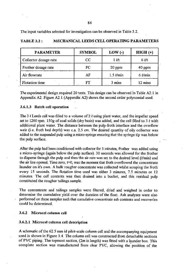
84

The input variables selected for investigation can be observed in Table 3 .2.

TABLE3.2: MECHANICAL LEEDS CELL OPERATING PARAMETERS

PARAMETER SYMBOL LOW(-) HIGH(+)

Collector dosage rate cc I Q/t 6 Q/t

Frother dosage rate FC 20ppm 40ppm

Air flowrate AF 1.5 Q/min 6 Q/min

Flotation time FT 3 mins 12 mins

The experimental design required 20 tests. This design can be observed in Table A2.1 in Appendix A2. Figure A2.1 (Appendix A2) shows the second order polynomial used.

3.6.1.3 Batch cell operation

The 3 Q Leeds cell was filled to a volume of 2 Q using plant water, and the impeller speed set to 1200 rpm. 150g of coal solids (dry basis) was added, and the cell filled to 3 Q with additional plant water. The distance between the pulp-froth interface and the overflow weir (i.e. froth bed depth) was c. a. 2.5 em. The desired quantity of oily collector was added to the suspended pulp using a wicro-syringe ensuri.ng that the syringe tip was below the pulp surface.

After the pulp had been conditioned with collector for 5 minutes, frother was added using a micro-syringe (again below the pulp surface). 30 seconds was allowed for the frother to disperse through the pulp and then the air rate was set to the desired level (Q/min) and the air line opened. Time zero, t=O, was the moment that froth overflowed the concentrate launder on it's own. A bulk rougher concentrate was collected whilst scraping the froth every 15 seconds. The. flotation time used was either 3 minutes, 7. 5 minutes or 12 minutes. The cell contents was then drained into a bucket, and this residual pulp constituted the rougher tailings sample.

The concentrate and tailings samples were filtered, dried and weighed in order to determine the cumulative yield over the duration of the float. Ash analyses were also performed on these samples such that cumulative concentrate ash contents and recoveries could be determined.

3.6.2 Microcel column cell

3.6.2.1 Microcel column cell description

A schematic.ofthe 62.5 mm id pilot-scale column cell and the accompanying equipment used is shown in Figure 3.4. The column cell was constructed from detachable sections of PVC piping. The topmost section, (2m in length) was fitted with a launder box. This complete section was manufactured from clear PVC, allowing the· position of the

85

pulp-froth interface to be visually monitored during column operation. The feed port was situated 1.30 m below the upper column overflow lip. Below this uppermost section, a 2.88 m length of PVC piping connects with the Microcel bubble generation system situated at the base of the column. The distance of the feed port to the sparger port, termed the collection zone, was fixed at 2.55 m. The sparger tip was positioned 0.33 m from the column base.

.------""'-""-, n'R,. Frolhwashing syslem

I Frolh supply

c ~- ....

0::! ··-----t-: ! Control

-:-::;~~wF-,.,..cl.!...l=...,g,=~ ; Platform

L ...... ____________ _ --------------------1 Air supplv to Mlcrocel Talis supply I

i Sparger Tailspt.!r.ip

Microcel Bubble Generation System

Figure 3.4 Schematic arrangement of the Microcel Column and equipment

The patented Microcel bubble generation system was purchased from MCT Blacksburg, Virginia, U.S.A. This unit comprised of a static mixer bubble generator encased in clear PVC with flange coupling for connection to the rest of the column. A variable speed motor rated to 2500 rpm was used to withdraw a portion of the column tails utilising this volume for bubble generation. This volume is related to the operating speed of the motor. A tee-connection positioned on the suction side ofthe pump allowed the balance ofthe tails to discharge from the column as final tails.

The air requirement was drawn from a compressor capable of delivering 7.5 bar pressure. The column air supply line was fitted with a pressure regulator assembly complete with moisture trap. A pressure gauge and rotameter were used to control the air flow to the air addition nozzle situated on the discharge side of the recycle line of the Microcel pump assembly.

The washwater distributor was constructed from 6mm outer diameter stainless steel tubing. From a vertical perspective the distributor consisted of a single branch 3.5 em in length adjoining the circular outer ring. Two lmm equally spaced holes were drilled in the

86

bottom face of the branch and the outer ring had 16 equally spaced I mm holes. The distributor was positioned 1 Ocm into the froth zone.

Water was supplied to the washwater distributor via a rotameter capable of maintaining flows upto 2 Q/min. The water supply to the column was first pressurised to 4 bar using a recycle pump coupled to a reservoir utilising a ball valve for- volume control and maintained at that pressure in order to avoid any line pressure drop which may occur when utilising the water utility line.

Differences in the electrical conductivities of the pulp (strong electrolyte) and froth (weak electrolyte) formed the basis for pulp level measurement. A 2m length of chrome/nickel wire complete with stainless steel probes (100mm apart) extended into the clear PVC section. A voltage was applied, and the voltage drop across the system is a function of the position of the pulp along the chrome/nickel electrode. An electronic controller receives the measured voltage signal, and executing a PI control alogarithm, varied the tailings pump speed in order to maintain the desired pump level. A variable speed Watson/Marlowe peristaltic pump capable of delivering flowrates upto 30 Q/min was used as tailings pump.

The frother requirement was drawn from a variable speed pump capable of delivering flows upto I Q/min. Frother was pumped continuously from a 10 Q container directly into the column, entering at the base and passing through the Microcel sparger. The pulp conditioning tank had a capacity of 100 Q, and was continuously agitated by a high pressure mono-circulation pump. The column feed was drawn from this vessel by means of a variable speed Watson/Marlowe peristaltic pump capable offlows upto IO e/min.

The launder box situated at the head of the column was fitted with a launder wash assembly. This consisted of a stainless steel tube, 'u-shaped', having 1mm holes drilled at Icm intervals across its entire length. The entire assembly was housed c. a. Scm above the sloping launder box. Launder washwater was supplied in exactly the same manner as that for the washwater distributor, except that a separate rotameter was utilised for flow control of this stream. The reason for incorporation of the launder wash stream was to gently wash the concentrate solids from the launder box to minimise errors during sampling. This volumetric flowrate of water was then subtracted from the wet sample mass in order to calculate the actual concentrate production rate.

3.6.2.2 Microcel column testing

· Parameters which were not varied or otherwise not controlled during the test programme are shown in Table 3.3.

87

TABLE3.3: CONSTANT AND UNCONTROLLED OPERATING PARA­METERS FOR THE MICROCEL COLUMN

PARAMETER VALUE

Inner Column Diameter 6.25 em

Feed Point distance below top overflop lip 1.30 m

Distance of water distributor below overflow lip 10.00 em

Launder washwater rate 1 Q/min

Percentage Solids (%) . 5%m/v

Collection zone height 2.55 m

Microcel pump pressure 100 kpa.

The input variables selected for investigation can be observed in Table: 3.4.

TABLE 3.4: MICROCEL COLUMN OPERATING PARAMETERS

PARAMETER SYMBOL LOW(-) HIGH(+)

Froth height FH 0.35 m 0.55 m

Collector dosage rate cc 1 Q/t 6 Q/t

Frother dosage rate FC 200 g/t 400 g/t

Air flowrate Qg 4.00 Q/min. 6.00 Q/min Jg 2.17 cm/s 3.26 cm/s

Slurry feedrate Qf 0.74 Q/min 1.47 Q/min Jf 0.40 cm/s 0.80 cm/s

Washwater rate Qw 0.53 Q/min 0.81 Q/min Jw 0.29 cm/s 0.44 cm/s

Superficial gas rates and wash water rates for the purpose of this thesis lie within the limits recommended by Yianatos, 1989 (see Table 3.5 below). The superficial slurry feed rate limits recommended by Yianatos, 1989 relate to column feed production rates of 1.8-3.6 t/hr/m2 which are typical for northern hemisphere coals. Van Holt, (1992) found that column feed production rates for southern hemisphere coal range between 0.5 -1.5 t/hr/m2

. This is the range selected here.

88

TABLE 3.5: TYPICAL FLOTATION COLUMN OPERATING PARAMETER VALUES, FROM (YIANA TOS, 1989)

OPERATING PARAMETER VALUE

Superficial gas rate, Jg I- 3 cm/s

Superficial wash water rate, Jw 0.3 - 0.5 cm/s

Superficial slurry rate, lr I- 2 cm/s

Furthermore, Van Holt (I992) recommends froth heights of 0.35-0.75 m for South Afiican coals. Yoon, (I990), reports that bubble size reduces dramatically by increasing the Microcel circulation speed. The selection of2500 rpm yielding a pressure of 100 kpa, relates to I 00% of the Microcel pump power setting. The collector dosage range selected is currently arbitrary. Typically, when evaluating columns, the optimum or standard collector dosage remains fixed since this is normally an economic constraint.

The column height/slurry combinations were selected to cover a broad spectrum of particle residence times. On the basis of column height (CH) = 2.55 m, Qr= 1.47 ~/min, net washwater rate= 0.53 Nmin, a minimum slurry nominal residence time of 1min = 3.91 minutes can be expected. Conversely, operating conditions of CH = 2. 55, Qf = 0. 7 4 ~/min,

and washwater rate= 0.53 Nmin would impart a maximum nominal slurry residence time of 1max = 6.16 minutes.

The experimental design required 31 tests. This design can be observed in Table A2.2, given in Appendix A2.

Sample formulae used in the conversion of the volumetric flowrates to superficial velocities, calculation of the cell production rate, and nominal slurry residence time are given in Appendix E 1.

3.6.2.3 Microcel column operation

At the start of a run, the feed conditioning tank (100 ~ capacity) was filled with plant water to the desired level (using a dip-stick), and coal added in order to make-up a slurry containing 5% solids m/v. The pulp density ofthe slurry was measured after 5 minutes agitation of the pulp using a Marsy scale and adjustments to the pulp density were made if required. As explained earlier, this vessel also served as the collector conditioning vessel. Due to the factorial experimental designs requirement of tests to be conducted with a high degree of randomness, only sufficient slurry was prepared for the completion of a single test. (i.e. slurry density is fixed at 5% for all tests but collector dosage (Uton) is varied). Collector was added to this vessel as required and dispersed largely via bulk turbulence for a period of 5 minutes.

89

Once the collector had been added to the slurry, the wash water and launder wash water rates were set to the required rate, allowing the Microcel column cell to be filled with water. The Microcel bubble-generator pump was switched o~:and set to 100% of the power setting yielding the required 100 kpa circulation pressure required. The required air rate (at 2 bar pressure) was adjusted to the desired flow on the air rotameter.

The required frother dosage was added continuously to the column from a make-up bucket (0.01% solution), and pumped at the required rate to the frother nipple situated on the suction side ofthe Microcel circulation p~mp at the base of the column.

The peristaltic pump feeding the column was switched on. The tailings peristaltic pump was then also switched on (manual setting), and set at a low flow-rate in order to prevent solids settling at the base of the column cell. Once the slurry volume in the column reached the 2 bottommost probes in the upper clear PVC section, the level control system was switched to the desired setting, and the tailings pump set to automatic using a PLC control unit.

After stable operation had been achieved, (approximately, three nominal cell residence times to reach steady state), the cell was sampled. Timed concentrate and tailings samples were taken simultaneously. The operating conditions were then changed and the system allowed to reach a new steady state before further samples were taken.

3.6.3 Jameson Cell

3.6.3.1 .Jameson cell description

A schematic layout of the Jameson cell test equipment which was used in the investigation is presented in Figure 3. 5.

SOLIDS WilER

MIXING 'D.HK WITH

STIRRER

Figure 3.5

PEI!!:O AlA INTAKE

\IUYe

DISCARO

Schematic of the Jameson cell and accompanying equipment

90

The coal feed was made up to a 5% sluny in the 100 Q pulp conditioning tank. A 1000 J.lm laboratory sieve was fitted to this tank in order to remove any tramp oversize aminating from the pulp merely as a precautionary measure in order to avoid orifice blockage.

The collector requirements were accurately dosed to the feed pulp and continuously agitated using a mono-circulation pump. This pump was capable of delivering 250kpa pressure at the rllixing head, and the static head was typically± 4.0 m. The Jameson cell feed was also drawn from this vessel by means of the high-pressure mono-circulation pump. The feed pressure to the Jameson cell was controlled by monitoring the feed pressure gauge (250kpa maximum), and manual adjustment of a gate valve situated on the discharge side ofthe pump.

The Jameson cell test unit consisted of a 4m downcomer, manufactured from clear PVC (25mrn id and 30mm od). The orifice situated at the head of the downcomer had a 4mm opening, manufactured from stainless steel. The feed capacity was approximately 6.67 Q/min at a jet velocity of about 15.6 mls. A .146mm inner diameter cell was used together .with a 90mm id displacement unit having heights of0.9 min order to evaluate the effect of a varying superficial air rise velocity Jg.

Froth level control was via a flexible hose that could be set at varying levels by lifting or lowering the position of the tailing outlet along its runner.

The air supply to the Jameson cell was naturally induced, by adding a sufficient amount offrother to the pulp (see Figure 2.23). This was necessary so that the jet ensuing from the orifice plate can entrain sufficient air to let the downcomer function properly. The test unit was fitted with an air rotameter capable of measuring flows of up to 10 Q/min. Vacuum and air supply were connected in series, with one control valve, which means that closing the air regulator valve, leads to an increase in vacuum. Both the air rotameter and magnahelic vacuum gauge (0-30 kpa) were fitted to a control panel in close proximity to the test unit.

Water was supplied to the washwater distributor via a rotameter capable of maintaining flows upto 2 Nmin. The water supply to the Jameson cell was first pressurised to 4 bar using a mono-recycle pump coupled to a reservoir utilising a ball valve for volume control and maintained at that pressure in order to avoid any line pressure drop which may occur when utilising the water utility line.

Washwater was distributed over the froth by a distribution pipe system and was measured by a rotameter on the control panel. The washwater trays were manufactured from HDPE, and lmm holes are drilled at lcm distances, evenly spaced across the entire tray area.

A launder box situated at the head of the cell for concentrate collection, was fitted with a launder wash assembly. This consisted of a stainless steel tube, 'U- shaped', having lmm holes drilled at lcm intervals across its entire length. The entire assembly was housed c. a. Scm above the sloping launder box. Launder washwater was supplied in exactly the same manner as that for the washwater distributor, except that a separate rotameter was utilised for flow control of this stream. The reason for incorporation of the launder wash stream

91

was to gently wash the concentrate solids from the launder box such that errors during sampling may be minimised. This volumetric flowrate of water was then subtracted from the wet sample mass in order to calculate the actual concentrate production rate.

3.6.3.2 Jameson cell testing using experimental designs

Parameters which were not varied or otherwise not controlled during the test programme are shown in Table 3.6.

TABLE 3.6: CONSTANT AND UNCONTROLLED OPERATING PARA­METERS FOR THE JAMESON CELL

PARAMETER ~ VALUE

Downcomer column inner diameter 25.4 mm -!!10:

Size of orifice 4.00mm

Launder washwater rate 1 ~/min

Feed % solids 5 %rnlv

The input variables selected for investigation can be observed in Table 3.7.

TABLE 3.7: JAMESON CELL OPERATING PARAMETERS

PARAMETER SYMBOL LOW(-) HIGH(+)

Froth height FH 0.15 m 0.50m

Collector dosage cc 1 Q/ton 6 Q/ton

Air flowrate AF 4 Q/min 8 Q/min

Frother additional rate FAR 200 ppm 400 ppm

Feed pressure FP 110 kpa 165 kpa

Washwater rate ww 0.95 Q/min 1.45 ~/min

The Jameson cell height/slurry combinations are selected to cover a broad spectrum of particle residence times. On the basis of column height (CH) = 4.0 m, feed pressure= 120 kpa Q,= 6.1 Q/min; net washwater rate Qw= 0 Q/min, a minimum slurry nominal residence time of 1min = 7.9 seconds can be expected in the downcomer. Conversely, operating conditions ofCH = 4.0, Q.= 7.10 Q/min, (180 kpa pressure), and washwater rate Qw = 3.0 Q/min would impart a maximum nominal slurry residence time of 1max = 12 seconds in the downcomer.

92

The experimental design required 31 tests. This design can be obseiVed in Table A2.3 in Appendix A2.

3.6.3.3 Jameson cell operation

At the start of a run, the feed conditioning tank (100 Q capacity) was filled with plant water to the desired level (using a dip-stick), and coal added in order to make-up a slurry containing 5% solids rn/v. The pulp density of the slurry was measured after 5 minutes agitation of the pulp using a Marsy scale and adjustments to the pulp density were made as required.

The wash water and launder wash water rates were set to the required rate, allowing the Jameson cell to be filled with water. The froth height level was set at the desired operating level by lifting or lowering the position of the tailing outlet along its runner. (This is calibrated.) The required collector was added from a syringe as a one-off dosage and the pulp conditioned for a further 5 minutes by continuously agitating the pulp using the high pressure mono-circulation pump. The feed valve to the Jameson cell was isolated during this conditioning period.

Five minutes after reagent-conditioning, the feed valve to the Jameson cell was fully opened and the pump recycle valve manipulated until the required test pressure of the feed supply to the Jameson cell had been obtained. At the same instant, the calibrated frother reagent pump was switched on. The Jameson cell tails pump (variable speed) was set to maintain a constant operating volume in the tails sump. This setting maintained a low flow rate in order to prevent the base of the cell from becoming blocked by settling solids. The tails discharged to a 2000 Q capacity holding tank.

When the cell had filled with slurry to the desired pulp level, air was introduced into the cell by opening the rotameter on the air line, and adjusting it to give the desired flow rate.

After stable operation had been achieved, (approximately, three nominal cell residence times to reach steady state), the cell was sampled. Timed concentrate and tailings samples were taken simultaneously. The operating conditions were then changed and the system allowed to reach a new steady state before further samples were taken.

Single-stage Jameson cell flotation was also conducted using deslimed Twistdraai (<300f.1m x 38J.1m) fine coal. In this case the collector concentration was fixed at a dosage of Hit for all tests. The experimental design in this case required 20 tests. This design can be obseJVed in Table A2.4 in Appendix A2.

3.6.4 Double-stage flotation

The motivation behind conducting two-stage flotation was to ascertain whether the ash content could be further reduced when using the optimum single-stage settings for both the Leeds mechanical cell and Jameson cell when treating (850f.1m x 0) Twistdraai fine coal. Furthermore, ash-by-size deportment results obtained from the cleaner flotation products would indicate if differences in preferential size class recovery was occurring

93

with these two flotation devices. In addition, efficiency testing would also be conducted using the samples data generated from the two-step flotation testwork in order to describe froth flotation in terms ofthe ecart probable (epm).

The operating conditions for both single-stage and two-stage flotation for both the Jameson cell and Mechanical cell can be observed in Tables.D7.1 and D7.2 respectively given in the Appendix D7.

For both of these experiments, the process conditions for the second-stage were selected in order to maximise concentrate yield whilst improving grade. Unfortunately, additional frother was required in both cases in order to promote a stable froth phase. In the case of the Jameson cell, the froth depth was decre~ed to 32.5cm from 50cm in the second- stage in order to obtain a concentrate, since no froth overflowed the cell at a setting of 50cm.

94

CHAPTER4

RESULTS AND DISCUSSION : GRAVITY CONCENTRATION TESTWORK

4.1 INTRODUCTION

As stated in section 1.3 earlier, the principal aim of this thesis is to develop a fine coal circuit capable of producing a 10% ash product for the Twistdraai Colliery. In essence, this project seeks to investigate whether gravity concentration, column-type flotation technology, or a combination ofthese; can be successfully used to recover a saleable (10% ash) coal product from the naturally-fine (<850Jlm x 0) Twistdraai Colliery fines.

From the literature reviewed in section 2.7 of this thesis, the (LD) spiral concentrator and the Stokes upward-current washer were chosen as gravity concentration equipment for investigation at the Twistdraai Colliery. This chapter describes the results of this gravity concentration testwork performed on a coal sample sized between (<850Jlm x 106Jlm) tested at the Twistdraai 150tph pilot plant facility in Secunda. Chapter 5 of this thesis describes the results of the froth flotation testwork.

Chapter 4 begins by reporting the feed coal characterisation results. This is followed by a discussion of both single and two-stage spiral and Stokes upward-current washer test results, and the chapter concludes with a summary.

4.2 CHARACTERISATION RESULTS

Feed coal characterisation studies conducted for this phase of the project consisted of: proximate, ultimate and petrographic analysis. In addition, feed washability, yield- by-size and ash-by-size testing for both single-stage and two-stage gravity concentrator circuits were also conducted. These results are given below.

4.2.1 Ultimate, proximate and petrographic analysis results

The ultimate analysis, proximate analysis and petrographic analysis results obtained for the Twistdraai fine coal composite sample (850Jlm x 106Jlm) are shown in Table 4.1 below.

From Table 4.1 it can be seen that the Twistdraai fine coal contains 49.0% fixed carbon, 21.9% volatile matter, 25.8% ash and 0.8% sulphur. It is also clear from the petrographic analysis that this coal contains 30% reactive semi-fusinite, 26.7% inertinite, 24% vitrinite and l% exinite. The reflectance ofvitrinite (RoV) measurement of0.7 indicate that this coal is ofbituminous rank..

95

TABLE 4.1: ULTIMATE, PROXIMATE AND PETROGRAPHIC ANALYSIS RESULTS FOR THE TWISTDRAAI (850J1m x 10611m) FINE COAL COMPOSITE

ULTIMATE ANALYSIS(% Dry, Ash Free).

c H N s 0

83.3 4.5 2.4 0.8 9.0

PRO~TE ANALYSIS(%)

Moisture Volatile Matter Ash Fixed Carbon

3.3 21.9 25.8 49.0

PETROGRAPHIC ANALYSIS(%)

Vitrinite Exinite -.~, RSF Inertinite Minerals Rank (RoV)

24.0 1.0 30.1 26.7 18.2 0.7

4.2.2 Single-stage circuit feed characterisation results

4.2.2.1 Washability results

Washability results for the single-stage gravity circuit feed is given in Figure 4 .1.

10

20

£l 30 :g u: 40 #. g! 50 ~ "3 60 E 8 70

Relative Density 2 1.95 1.9 1.85 1.8 1.75 1.7 1.65 1.6 1.55 1.5 1.45

---------~ -------------------------------- ---- --1 I

_________ JL__ ----------------------------- --------l I I I I I I I

80L---+~.....---~c-90

1.4

100

90

80

70

60

50

40

30

20

10

100~~~;r~~~~~~~~~~~~~~~~~~j 0 20 30 40 50 60 70

Cumulative Ash %

I• FlostLine • DensimetricLine + DifficuiltyLine

"' .>< c:

Ci)

?F. CD

~ ... "3 E ;:J

0

Figure 4.1 · Densimetric, Difficulty and Cumulative floats curves for the primary-stage gravity circuit feed (Twistdraai 8S011m x 0 fine coal composite)

96

It can be observed from Figure 4.1 that a yield of 3 6% can be obtained theoretically at 10% ash. The densimetric and difficulty cuiVes for this feed sample also indicate that a d50

or cut-point of 1,55 is required in obtaining a 10% ash. Furthermore, a significant amount (46%) of near-density (0.1 RD) material is present at this cut-point indicating that gravity separation would be extremely challenging. The washability data for this sample is given in Appendix C2.1.

4.2.2.2 Yield-by-size and ash-by-size results

Three single-stage test runs were conducted with both the Spiral and Stokes devices. These tests were designated sample identifications of 1.12~ 1.13 and 1. 15. In the case of run 1.12 for example, samples were taken for both devices in a simultaneous manner, thereby sharing a common feed or head sample. This same approach was used for all other tests.

Cumulative yield-by-size and ash-by-size results for the three single-stage feed samples having washability characteristics reported in section 4.2.2.1 can be observed in Figures 4.2 and 4.3 respectively. Test run 1.13 feed constituted the normal plant splitter position setting, and contained 25.8% ash. From these results . it is clear that the plant feed consistency varied. This variance is discussed below.

- 80 ~ '--' '"0 Q) •;>..

(1,) ;> 60 ·-~ 1 8

40

Run 1.12 Yield Run 1.13 Y"l&ld Run 1.15 Yield

• 0

20 ~--------~------~-------L------~~------~ +500

Figure 4.2

+300 +212 +150 particle size (J..lm)

+106 -106

Primary Spiral circuit feed consistency results showing cumulative yield by size data for the 3 test runs

97

~~---------------------------------------.

32

_., ~ 30 ..c: ell ~

~ 28 ·.g ] 26 ::s­o

24

22

Run 1.12Ash Run 1.13Ash Run 1.15Ash

• 0

20 ~------~--------L-------~-------L------~ +500 +300 +212 +150 +106 -106

particle size (Jlm)

Figure 4.3 Primary Spiral circuit feed consistency results showing cumulative ash distribution by size data for the 3 test runs

Calculated averages and standard deviation results for both yield and ash are given in Table C3 .1 in Appendix C3.

Clearly the ash content of test 1.12 .is considerably higher than that of the other 2 test runs, thus causing this large deviation. For test 1.12, care must be taken in interpreting the results and should not be used in formulating any conclusions.

4.2.3 Two-stage circuit feed characterisation results

4.2.3.1 Washability results

Washability results for the two-stage circuit feed (spiral product from test 1.13 in section 4.4.1 below) is given in Figure 4.4.

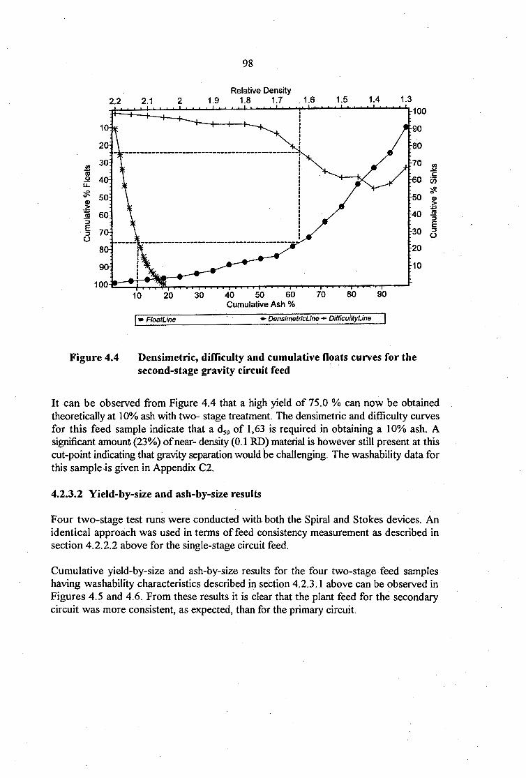
98

Relative Density 2.2 2.1 2 1.9 1.8 1.7 1.6 1.5 1.4 1.3

100

90

80 - ----------------------------------------------.

1/)

a; 0 u: eft 50 Q) >

".;:> 60 IV 3 E 70 ·::s ()

80

90

Figure 4.4

10 20 30

!• FloatLine

40 50 60 Cumulative Ash %

I I I

70 80

• DensimetricLine + Difficui/tyUne

70

60

50

40

30

20

10

90

Densimetric, difficulty and cumulative floats curves for the second-stage gravity circuit feed

1/) .l<: c

Ci5 ~ 0

Q)

.2: a; 3 E ::s 0

It can be observed from Figure 4.4 that a high yield of 75.0 % can now be obtained theoretically at 10% ash with two- stage treatment. The densimetric and difficulty curves for this feed sample indicate that a d50 of 1,63 is required in obtaining a 10% ash. A significant amount (23%) ofnear- density (0.1 RD) material is however still present at this cut-point indicating that gravity separation would be challenging. The washability data for this sample .is given in Appendix C2.

4.2.3.2 Yield-by-size and ash-by-size results

Four two-stage test runs were conducted with both the Spiral and Stokes devices. An identical approach was used in terms of feed consistency measurement as described in section 4.2.22 above for the single-stage circuit feed. .

Cumulative yield-by-size and ash-by-size results for the four two-stage feed samples having washability characteristics described in section 4.2.3.1 above can be observed in Figures 4.5 and 4.6. From these results it is clear that the plant feed for the secondary circuit was more consistent, as expected, than for the primary circuit.

-.. ~ "-" "'0 v •;>.. (!)

> ·-~ "3 s ::s u

99

80

60

40

Run1.12Yield Run1.13Yield Run1.14Yield Run1.15Yield

• 0

20 ~--------L-------~------~------~--------~ +500 +300 +212 +150 +106 -106

particle size (J.lm)

Figure 4.5 Secondary Spiral circuit feed consistancy results showing cumulative yield by size data for the 4 test runs

20 .--------------------------------------------. Run 1.12Ash Run 1.13Ash Run 1.14Ash Run 1.15Ash

• 0 19

14 LL------~L-------~-------L------~--------~ +500 +300 +212 +150 +106 -106

particle size (J.lm)

Figure 4.6 Secondary Spiral circuit feed consistancy results showing cumulative ash 'distribution by size data for the 4 test runs

100

Calculated averages and standard deviation results for both yield and ash for the two-stage circuit are given in Table C3 .2 in the appendix. It can be observed that the (SD) results for cumulative yield peak at 1.9 which is an indication oflow variance. Cumulative ash variance was even lower, i.e. (SD's) of c. a 0.4 were obtained which implies a high degree of feed consistency between tests.

4.3 Single-stage circuit test results

All samples produced in the gravity concentration testwork were wet screened at 500!-lm, 212!-lm, 150!-lm and 10611m. These fractions were dried at 85°C, weighed and ashed. In this way, the effect of desliming of the product obtained could be investigated.

4.3.1 Single-stage spiral circuit results

Yield and ash distribution results obtained for the three single-stage spiral circuit tests conducted are summarised in Table 4.2. Detailed yield and ash distribution by size data for these tests are given in Tables C3.3 to C3.5 in Appendix C3.

TABLE 4.2: SUMMARY OF THE YIELD AND ASH DISTRIBUTION RESULTS OBTAINED FOR THE SINGLE-STAGE SPIRAL TESTS

PRODUCT DISCARD FEED

TEST Yield Cum. Ash Cum. Yield Cum. Ash Cum. Ash Cum. (%) (%) (%) (%) (%)

1.12 64.7 18.9 35.3 59.9 33.4

1.13 81.7 19.1 18.3 55.7 25.8

1.15 7·7.9 19.3 22.1 59.0 28.1

It can be seen from Table 4.2 that the feed ash content varied between 25.8% and 33.4% for these tests, and a significant proportion of the feed consisted of ultrafine (misplaced) <106!-lm material (Tables C3.3 to C3.5). Clearly, the classifying cyclone ahead of the single-stage Spiral circuit was not operating very efficiently leading to a high percentage (12.8%-16.4%) ofthe Spiral feed coal consisting of<106!lm ultrafines. These ultrafines also had an ash content ranging between 40.3% and 51.6%, thereby increasing the overall feed ash content by about 3% in this circuit.

The single-stage Spiral product grade obtained ranged between 18.9% and 19.1% ash for these tests, from a feed ash ranging between 25.8% and 33.4%. The standard plant operating splitter position (test 1.13) yielded a product ash of 19.1% at a product yield of 81.7%. Varying the Spiral splitter position did not influence the product ash significantly, but, yields were affected, ranging between 64.7% and 81. 7%. Again the negative influence of the ultrafine <1061-lm fraction can be observed on the resultant product grade.

101

Discard ash content for these tests varied between 55.7% and 59.9%. Surprisingly, the primary Spiral discard contained c.a. 16.5% <l0611m material, indicating that this device is capable of rejecting ultrafines on the basis of density. Furthermore, coarse +5001lm discards contributed about 15% to this fraction, but contained c.a. 62% ash.

4.3.2 Single-stage stokes upward-current washer results

Yield and ash distribution results obtained for the three single-stage Stokes upward current washer tests conducted are summarised in Table 4.3. Detailed yield and ash distribution by size data for these tests are given in Tables C4.1 to C4.3 in Appendix C4.

TABLE 4.3: SUMMARY OF THE YIELD AND ASH DISTRIBUTION RESULTS OBTAINED FOR THE SINGLE-STAGE STOKES SEPARATOR

PRODUCT DISCARD FEED

TEST Yield Cum. Ash Cum. Yield Cum. Ash Cum. Ash Cum. (%) (%) (%) (%) (%)

1.12 37.8 23.7 62.2 39.3 33.4

1.13 82.5 23.7 17.6 35.6 25.8

1.15 59.5 20.8 40.5 38.8 28.1

It may be observed from Table 4.3 that the product grade obtained ranged between 20.8% and 23.7% ash for these tests, and the best result (test 1.15) produced a product grade of20.8% at 60% product yield. The negative influence ofthe ultrafine <1061lm fraction can again be observed on the resultant product grade. Furthermore, since the Stokes device is also considered a hydrosizer, the ultrafine <1 06J.lm fraction reported almost in its entirety (99%) to the product, as expected (Tables C4.1 to C4.3).

The discard ash contents for these tests varied between 35.6% and 39.3%, and in general, this discard contained c.a. 80% +500!lm material containing c.a. 35% ash. This implies that this device has difficulty in rejecting only high ash coarse material. Again the ability of this device to act as a sizer is very pronounced.

4.3.3 Comparison of the single-stage Spiral and Upward-current washer test results

A comparison of the separation performance achieved from the in-plant testing of the existing single-stage Spiral circuit and the Stokes upward-current washer in terms of combustible recovery vs ash rejection is shown in Figure 4.7. Sample formulae for calculating both combustible recovery and ash rejection are given in Appendix E1.

102

100 .---~----------~--------------------------~

90

cao Q)

> 0 0

~ ~.70 .0 ·.;z "-' :s

.0

E so 0 0

50

• 1.15

; Stokes

-II---+- • 1.12 40 L---~--L---L---L---~~~~--~--~--~--~--~

20

Figure 4.7

30 40 50 60 70 80 ash rejection (%)

Comparison of the separation performance achieved from the in-plant testing of the existing primary Spiral circuit and the Stokes upward current washer

From Figure 4.7, it can be observed that the spiral yielded more than a 10% increase in combustible recovery at similar ash rejection when compared to the Stokes upward-current washer during in-line single-stage testing. A possible explanation as to why the spiral achieved superior separation performance is given below.

The Stokes upward-current washer behaved as a sizing device in that 99% of the misplaced <1 06Jlm coal present in the feed reported to the concentrate, thereby masking · the product grade negatively. Conversely, the spiral discard contained c.a. 16.5% <106Jlm material, indicating that this device was capable of rejecting ultrafines on the basis of density. Furthermore, the discard ash content of the Stokes concentrator contained c.a. 80% +500Jlm material containing c.a. 35% ash, implying that this device has difficulty in rejecting only high ash coarse material. The average discard ash content was 60% and 38% for the Spiral and Stokes concentrator respectively.

In a recent in-plant investigation (Honaker, 1996) states that both the Floatex and Stokes density separators provide an efficient alternative to current technologies such as Spirals when treating Illinois no 6 seam coal, and that this advantage may only be applicable to coals having easy- to-clean characteristics due to their high relative density cut-points. The current Twistdraai colliery findings are in agreement with Honaker~ since the near-density (0.1 RD) ofthe Twistdraai coal at a probable error of0.1 approaches 47 %.

103

In conclusion, neither gravity concentration device was capable of reducing the product ash content to 10% in a single-stage, and two-stage circuit testing is necessary to further reduce the product ash content to the requirement of 10% ash.

4.4 TWO-STAGE CIRCUIT TEST RESULTS

In section 3. 5.1, it was explained that the product and middling of the primary spiral circuit were combined as feed to the secondary spiral circuit. Conversely, the middling and discard of the secondary spiral circuit were combined as a single reject.

4.4.1 Two-stage spiral circuit results

Yield and ash distribution results obtained for the four two-stage spiral circuit tests conducted are summarised in Table 4.4. Detailed yield and ash distribution by size data for these tests are given in Tables C3.6 to C3.9 in Appendix C3 ..

TABLE 4.4: SUMMARY OF THE YIELD AND ASH DISTRIBUTION RESULTS OBTAINED FOR THE TWO-STAGE SPIRAL TESTS

PRODUCT DISCARD FEED

TEST Yield Cum. Ash Cum. Yield Cum. Ash Cum. Ash Cum. (%) (%) (%) (%) (%)

1.12 34.5 15.8 65.5 20.8 19.1

1.13 79.5 16.2 20.5 25.3 18.0

1.14 76.5 15.6 23.5 30.0 19.0

1.15 76.8 16.7 23.2 29.4 19.7

It may be observed from Table 4.4 that the feed ash content varied between 18.0% and 19.7% for these tests, and a significant proportion of the two-stage circuit feed consisted ofultrafine (misplaced) <106~m material. This fraction ranged between 15% and 18% of the total feed. These ultrafines have an ash content of c.a. 36%, thereby increasing the overall feed ash content by about 3% in this circuit (Tables C3.6 to C3.9).

Product grade obtained ranged between 15.6% and 16.7%, and the standard plant operating splitter position (test 1.13) yielded a product ash of 16.2% at a product yield of 79.5%. Varying the spiral splitter position did not influence the product ash significantly, but, yields were affected, ranging between 34.5% and 79.5%. The negative influence of the ultrafine <106~m fraction can be observed on the resultant product grade (Tables C3.6 to C3.9).

104

Discard ash content obtained for these tests varied between 20.8% and 30.0%, and the discard contained c.a.12% <1 06J1m material, indicating that this device was capable of rejecting ultrafines on the basis of density. Furthermore, coarse +500Jlm discards contributed within the range of 16% and 56% to this fraction. Likewise, the ash contents varied between 13% and 31%. These differences obtained can be ascribed to manipulation of the spiral splitter position, thereby shifting the grade/recovery curve.

4.4.2 Two-stage Stokes upward-current washer circuit results

Yield and ash distribution results obtained for the four two-stage Stokes separator tests conducted are summarised in Table 4.5. Detailed yield and ash distribution by size data for these tests are given in Tables C4.4 to C4.7 in the Appendix C4.

TABLE 4.5: SUMMARY OF THE YIELD AND ASH DISTRffiUTION RESULTS OBTAINED FOR THE TWO-STAGE STOKES SEPARATOR

PRODUCT DISCARD FEED

TEST Yield Cum. Ash Cum. Yield Cum. Ash Cum. Ash Cum. (%) (%) (%) (%) (%)

1.12 76.8 18.2 23.0 22.0 19.1

1.13 94.1 17.8 5.9 21.6 18.0

1.14 72.2 17.9 27.8 21.7 19.0

1.15 89.8 19.0 10.2 26.0 19.7

It may be observed from Table 4.5 that the product grade ranged between 17.8% and 19.0%, and the best result (test 1.13) generated a product grade of 17.8% and 94.1% product yield. The negative influence of the ultrafine <106Jlm fraction can again be observed on the resultant product grade since this fraction reported in its entirety to the product. Again the influence of this device to act as a sizer is very pronounced. (Tables C4.4 to C4.7).

The discard ash content varied between 21.6% and 26.0% for these tests and contained c.a. 92% +500Jlm material at c.a. 22% ash. This again implies that this device has difficulty in rejecting only high ash coarse material. (Tables C4.4 to C4.7).

4.4.3 The effect of desliming on the two-stage circuit

Clearly both devices were not capable of achieving a 10% product ash in the two-stage cleaner circuit. However, on inspection of the ash-by-size results for both devices (see Tables C3 .6 to C3 .9 and Tables C4.4 to C4. 7 in the appendix), a significant reduction in product ash is apparent in most size fractions.

105

Clearly, the option of des liming at 1 06flm (which is the typical Witbank coalfield practice) would not be practicable here since desliming ofthe spiral product at 106flm eg. (test 1.12) produces an overall yield of only 15.8% for both stages containing 10.3% ash. This yield is way below the 38% possible as predicted by washability and also slightly exceeds the 10.0% ash product constraint. Furthermore, spiral test 1.12 was regarded as questionable earlier due to it's high feed ash content, and should not be used in formulating conclusions. Regardless of this comment, both spirals as well as the Stokes separator could not achieve the required quality when deslimed at 1 06flm and inspection at other cut-sizes shouldbe investigated.

The effect of desliming for both devices in terms of cumulative product ash is graphically depicted in Figures 4.8 to 4.11. A clear trend which emerges for all4 comparative runs is that the Stokes upward-current washer produces a cleaner +300flm product fraction than does the Spiral.

Furthermore, by desliming the Stokes product at 300f.1m, the product ash is within the desired range of 10%. This observation does not hold entirely for the spiral, where only test 1.12 achieved an ash content lower than the target ash of 10% after desliming at 300f.1m (See detailed test results given in Tables C3.6 to C3.9). From these results, only 6% ash is present in the +500 flm fraction and the ash content increases steadily with a decrease in particle size.

In further support of the above statement, a graphical representation is given by Figure 4.12. This figure shows a comparison between the separation performance achieved from the in-plant testing of the existing two-stage Spiral circuit and the Stokes upward-current washer· in terms of combustible recovery vs ash rejection. In addition, the effect of desliming at 300f.1m for both devices is included. In this case these results are calculated as if there was no <300flm material present in the feed.

106

20 ~--------------------------------------~

18

---16~----~-----.------------'$. :;;'14 ~ ~12 -~

]10 g

8

6 Feed 1.12 Product (Stokes) Product (Spiral)

4 ~------~--------~------~------~--------~ +500 +300 +21~ +150

particle size(J.lm) +106 -106

Figure 4.8 Cumulative ash grade size comparison of the Stokes separator and the existing secondary Spiral circuit (Run 1.12)

20 ~------------------------------------~

l=~es) ~ral) 6 ~------~------~------~--------~------~ +500 +300 +212 +150

particle size(J.lm) +106 -106

Figure 4.9 Cumulative ash grade by size comparison of the · Stokes separator and the existing secondary Spiral circuit (Run 1.13)

107

20~-----------------------------------.

• •

Feed 1.14 Product (Stokes) Product (Spiral)

4~------~------~------~------~--------~ +500 +300 +212 +150 +106 -106

particle size(Jlm)

Figure 4.10 Cumulative ash grade by size comparison of the Stokes separator and the existing secondary Spiral circuit (Run 1.14)

22 .-------------~~----~----------------,

20

18

8

6 Feed 1.15 Product(Stokes); Product(Spiral)

--+--

4 ~------~--------~----~~------~------~ +500 +300 +212 4-150 +1 06 -106

particle size(Jlm) . I

I Figure 4.11 Cumulative ash grade by size comparison of the

Stokes separator and th¢ existing secondary Spiral circuit (Run L15) !

108

From observing the undeslimed grade/recovery curves shown in Figure 4.12, it again appears that the spiral produces a sharper separation when compared to the Stokes. However, upon desliming, the grade/recovery curve shifts as expected, since the high ash fraction for both devices is now removed. Furthermore, the ash rejection possible by desliming for the Stokes device is greater than for the Spiral at similar combustible recovery (see tests 1.13 Spiral and 1.15 Stokes).

The hypothetical desliming scenario presented in Figure 4.12 was then normalised by taking into account the percentage of+ 300Jlm materiat present in the undeslimed product, and is presented in Figure 4.13. In this case both gravity separators now achieve similar. grade-recovery curves on the two-stage cleaner circuit. Desliming of the product at 300Jlm in both cases increases the slope of the grade-recovery curve, indicating that it is the <300Jlm fraction which is responsible in not producing a 10% product ash. A significant increase in ash rejection can however be observed here in the case of the Stokes upward-current washer i.e. increasing from c. a. 20% on average for the undeslimed tests to c.a. 90% on average by desliming at 300Jlm. The spiral does not appear to show such a dramatic shift on desliming mainly because ultrafines are rejected into the discards, whereas the reverse is obtained with the Stokes.

1 100 .----------------------,

- 90 ~

>-a: 80 w > 0 frl 70 a: w

60 __J m l-en ~ 50 ~ 0 u 40

1.13

-~-1;..~- ---------------.--- ------- . -... ':":~?. ,~':, ................. .

---~-~ - - - - - - - -- - - -- -1-.,~ --- - - - -~ 1~- - - - - - - - - - -

. D. 1.15

. . . . . . . . . . . . . . '·'~~ ..... ------------- -- ----- -- -- ---- -~~~\D. --1.12

• 1.12 30~----_. _____ ~----~----~

0 20 40 60

ASH REJECTION (%)

SECONDARY SPIRAL NOT DESLIMED

STOKES NOT DESLIMED

.o • SECONDARY SPIRAL· STOKES DESLIMED AT 300um DESLIMED AT 300um

... D.

80

Figure 4.12 Combustible recovery and ash rejection data showing the hypothetical effect of desliming at 300p.m for both the existing Spiral circuit and Stokes separators

>­a:: ·W >

109

100~--~-----------------------------,

80

0 60 (..) ~~

' ' w a::

- -- - - --.. - - - ... :.. - -- .... -~ - - ..... - ":' - ~-.. ,· - -- ---- ... -'A.

& 20 . - - - - - - - - - - - - - - - - - -. - - - - - - - - - - - - - - - -~- -

0 0L-----~------~----~------8~o------,~oo 20 40 60

ASH REJECTION (%)

SECONDARY SPIRAL NOT DESLIMED

• STOKES

NOT DESLIMED 0

SECONDARY SPIRAL " STOKES " DESLIMED AT 300um DESLIMED AT 300um

... 6. • YIELD DISCOUNTED BY PERCENTAGE CONTRIBUTION

OF +300um PRESENT IN THE CONCENTRATE

Figure 4.13 Combustible recovery and ash rejection data showing the normalised effect of desliming at 300J.lm for both the existing spiral circuit and Stokes separators

From the aforementioned reasoning, it is clear that the desired product ash of 10% can be obtained upon desliming at 3001J.m. This however only represents between 11% and 30% of the total feed reporting to the Twistdraai fine coal circuit via the single-stage Spiral. Clearly, by rejecting the <3001J.m fraction to discard would represent a considerable loss in combustibles with associated revenue losses. It is therefore imperative that a recovery process, specific for the treatment of this fine <3001J.m fraction be implemented in order that maximum organic efficiencies are obtained, and that the final reject is still suitable for combustion at Sasol's steam plant at Secunda.

4.5 CHAPTER SUMMARY

For the single-stage gravity concentration circuit, the (LD) Spiral yielded a 10% increase in combustible recovery at similar ash rejection when compared to the Stokes upward­current washer. Neither device was however capable of achieving the required product ash of 10% in a single-stage, and two-stage treatment is advisable. On the basis of the single-stage results, selection of the (LD) Spiral over the Stokes upward-current washer is clearly justified providing that two-stage treatment yields the required metallurgy.

Both gravity separators achieved similar grade-recovery curves in the secondary circuit, but could still not attain the required quality. Ash-by-size measurements clearly indicated that the particle size distribution of the current feed size range fed to the existing spiral circuit (<8501J.m x 1061J.m) is incapable of producing a product below 10% ash.

llO

Clearly, the option of desliming at l06Jlm (which is the typical Witbank coalfield practice) would not be practicable here since desliming ofthe spiral product at 106Jlm eg. (test 1.12} produces an overall yield of only 15.8% for both stages containing 10.3% ash. This yield is way below the 38% possible as predicted by washability and also slightly exceeds the I 0.0% ash product constraint. Furthermore, spiral test 1.12 was regarded as questionable earlier due to it's high feed ash content, and should not be used in formulating conclusions. Regardless of this comment, both spirals as well as the Stokes separator could not achieve the required quality when deslimed at 1 06Jlm and inspection at other cut-sizes should be investigated.

The answer lies in desliming the cleaner product obtained from either a Spiral or Stokes separator at 300Jlm. This achieves the target ash of 10% at overall yields of between 11% and 30%. However, discarding of the -300Jlm fraction would be wasteful and uneconomic, and clearly indicates the need to investigate the treatment of this fraction via froth flotation.

111

CHAPTERS

RESULTS AND DISCUSSION: FROTH FLOTATION TESTWORK

5.1 INTRODUCTION

As stated in section 1.3, the principal aim of this thesis is to develop a fine coal circuit capable of producing a 10% ash product for the Twistdraai colliery. In Chapter 4 it was stated that both the LD Spiral and Stokes upward current washer gravity separators tested achieved similar grade-recovery curves in the two-stage circuit, but could still not attain the required product quality.

In Chapter 4 it was also shown that desliming of the cleaner two-stage gravity concentrator product (particularly in the case of the Stokes separator) at 300J.1m achieves the target ash of 10%, at overall yields of between 11% and 30%. Furthermore, discarding of this -300Jlm fraction would be wasteful and uneconomic, and the possibility of treating this fraction via froth flotation in order to improve organic efficiency in the Twistdraai fine coal circuit should be investigated.

From the literature reviewed in section 2. 7 of this thesis, the Microcel column flotation cell and the Jameson cell were chosen as froth flotation devices for investigation in this thesis. This chapter describes the results of the froth flotation testwork performed on two Twistdraai fine coal samples i.e. sized between {<850J.1m x 0) and (<300Jlm x 38J.1m).

Chapter 5 begins by reporting the feed coal characterisation results for both the (850J.1m x 0) and (300J.1m x 38Jlm) coal samples tested. This is followed by a discussion of the single-stage flotation results obtained for both of the coal samples in terms ofboth global and parameter effects. The chapter continues by discussing two-stage flotation and • efficiency testing results for the (850Jlm x 0) fine coal sample, and concludes with a chapter summary.

5.2 COAL SAMPLE CHARACTERISATION RESULTS

As stated in section 3 .2.1 coal characterisation studies were conducted on the froth flotation (850J.1m x 0) fine coal sample described in section 3.2.1.2. The 300J.1m x 38J.1m sample cut was produced by screening the coarse 850J.1m x 0 composite at 300J.1m, and desliming the <300J.1m size fraction at 38J.1m using a 100mm diameter classification cyclone.

The reason for testing of the -300Jlm x 38Jlm size fraction is as a result of the gravity concentration testwork results reported in Chapter 4 of this thesis, in which it was concluded that desliming of the two-stage Stokes upward-current washer product at 300J.1m produced the required grade of 10% ash at overall product yields of between 11% and 30%, but treatment of the -300J.1m fraction via froth flotation should be investigated in order to maximise combustible recovery in the Twistdraai fine coal circuit.

112

Furthermore, surface characterisation results reported in section 5.3 of this thesis clearly indicate that the ultrafine -38J!m slimes fraction appears detrimental to the froth flotation process since it contains significantly higher carboxylic acid functional groups and is more oxidised than the coarser +38J!m coal fraction.

Characterisation results reported in this section include: size and ash-by-size analysis, float-and-sink analysis, release flotation analysis, surface oxidation analysis, contact angle measurement and reagent screening results.

5.2.1 Size and ash-by-size results

5.2.1.1 Composite (850J.1m x 0) size fraction

The size distribution of the composite feed sample (850J!m x 0) and the ash content of each size fraction are presented in Table 5.1.

TABLE 5.1: ASH-BY-SIZE DISTRIBUTION DATA FOR THE COMPOSITE (850J.1m X 0) TWISTDRAAI FINE COAL SAMPLE

Size fraction mass percent in size ash content in (urn) Fraction(%) size fraction (%)

+500 25.2 33.3 -500+300 12.6 35.3 -300+212 8.9 23.5 -212+ 150 9.5 24.7

-150+106 5.8 25.9 -106+75 2.9 28.3 -75+45 5.0 31.8 -45+38 1.9 34.1 -38 28.2 36.0

Heap 100.0 32.0

The results in Table 5.1 show that the sample was relatively coarse, with a high proportion {56.2%) of+l50 Jlm material. Material ofthis size is generally difficult to beneficiate by flotation. Only 15.4% ofthe material was in the optimum flotation range of -150+38Jlm size fraction, with 28.2% of the feed finer than 38J!m.

The results ofthe ash determinations indicate that the <38J!m size fraction contained the highest fractional ash {36%). The overall ash content was 32.0%.

5.2.1.2 Deslimed (300um x 38um) size fraction

The size distribution of the deslimed feed sample {300J!m x 38J!m) and the ash content of each size fraction are presented in Table 5.2.

113

TABLE 5.2: ASH-BY-SIZE DISTRIBUTION DATA FOR THE DESLIMED (300J.1m x 38J.1m) TWISTDRAAI FINE COAL SAMPLE

SIZE FRACTION MASS PERCENT IN SIZE ASH CONTENT IN (J.lm) FRACTION(%) SIZE FRACTION (%)

-300+212 14.4 23.5 -212+150 18.6 24.7 -150+106 14.8 25.9 -106+75 14.4 28.3 -75+45 27.0 31.8 -45+38 8.5 34.1

-38 2.3 36.0

Head 100.0 28.2

The results given in Table 5.2 show that the desliming operation was very satisfactory with this feed now containing only 2.3% by mass of particles finer than 38!lm. Furthermore, the ash content increases as expected with a decrease in particle size, and the bulk cut contains only 28.2% ash.

5.2.2 Float-and-sink analysis results

The results of the float-and sink analysis of the froth flotation composite feed sample sized between 850!lm x 0 are graphically depicted in Figure 5.1. From these results it can be seen that the coal is not very well liberated in terms of it's relative density properties, and a theoretical yield of38% is indicated at an ash content of 10 %.

Float-and-sink analysis was not conducted for the deslimed (300J..lm x 38J..lm) fine coal sample.

5.2.3 Release flotation results

Release flotation analysis was conducted on the composite feed (850J..lm x 0 size fraction), as well as on a sample in the 300J..lm x 38J..lm size range, in order to obtain an indication of the optimum performance that could be achieved by froth flotation.

5.2.3.1 Composite (850J.1m x 0) size fraction

Release analysis results for the composite sample is given in Appendix C2, and graphically depicted in Figure 5.2. It can be observed from this data that the lowestash content obtained was 9 %, and a theoretical yield in the region of only 21 % was indicated at an ash content of 10%, compared to a value of 3 8 % indicated by float-and sink analysis reported for the same coal sample in section 5.2.2.

114

5.2.3.2 Deslimed (300J.1m x 38J.1m) size fraction

Release flotation analysis was conducted on the 1 OOmm diameter cyclone underflow sample to obtain an indication of the optimum performance that could be achieved by flotation on this fraction. Although desliming at 3 8 flm is not practised commercially, the aim of the thesis is to explore all of the possibilities and clearly efficient desliming is possible at this cut size (see Table 5.2).

The flotation release analysis results are also shown in Figure 5.2 together with the composite 850J.1m x 0 release results. It can be observed that the lowest ash content obtained was 9.6 %, and a theoretical yield in the region of29% was indicated at an ash content of 10%. Generally, it may be observed that the shape of the theoretical release curve for the deslimed coal sample is reasonably flat between the desired 10% ash and 12.5% ash levels, indicating that yields ranging from 29% up to about 65% should be reasonably easy to obtain.

Relative Density 2 1.95 1.9 1.85 1.8 1.75 1.7 1.65 1.6 1.55 1.5 1.45 1.4

10

20

.; 30 0 I U: 40 I ~ ----------~- -------------------------------------~ 50 I +:> I

~ 60 I

E 8 70

80L--+-.---~c-90

100~~~~~~~~~~~~~~~~~~~~~~~~~j 0 10 20 30 40 50 60 70

Cumulative Ash %

I•FioatUne + DensimetricLine + DifficuiltyLine

100

50

40

30

20

10

II) .ll: c en

?f. Q)

> 1ii '3 E ::I 0

Figure 5.1 Foat-and-sink data for the composite(850J.1m X 0 )Twistdraai fine coal sample

115

16 ----------------------------------------------------

~ 14 '-"

~ ~

t) ~ 12 ----------------- ----------------- ----------------

8 tl..

20

-~c~z~---P~~e-- -300,um x 3B,um 850,um x O,um

-----P1gduct yield (% ~O 80

Figure 5.2 Release flotation data for the Twistdraai (850p.m x 0) and (300p.m x 38p.m) fine coal samples

5.2.4 Surface oxidation results

Coal is an example of a heteropolar surface, since it contains· a hydrophobic carbon structure and hydrophylic mineral matter. It is important, however, that coal oxidation be kept to a minimum since oxygen-containing functional groups render the coal surface more hydrophylic thereby inhibiting cleaning by surface dependant processes like froth flotation.

5.2.4.1 Functional groups

The functional groups of the Twistdraai coal were characterised by size and results can be observed in Table 5.3.

TABLE5.3: FUNCI'IONAL GROUP CHARACI'ERISATION RESULTS FOR TWISTDRAAI FINE COAL

SIZE FRA.CfiON COOH TOTAL ACID GROUPS OH (MICRON) (%) (%) (%)

-500+300 0.15 0.54 4.61 -300+106 0.15 1.39 4.40 -106+75 0.16 0.50 3.72 -75+38 0.13 1.24 4.37.

-38 0.25 2.40 4.21 Calculated 0.18 1.03 4.34 Actual 0.25 0.98 4.12

116

The functional group content of the different coal fractions are the same with the exception ofthe -38~m fraction which has a relatively high carboxylic acid and total acid group content. This can be ascribed to the larger surface area of the ultrafine fraction containing a higher percentage of phenolic hydroxyl groups.

It can be expected that the -38~m fraction will be the most difficult to float since flotation is influenced mostly by the COOH acid groups. The coal fraction coarser than 38 micron has Jess oxygen groups on the surface and should react more favourably to flotation than -38~m fraction.

5.2.5 Contact angle measurement results

Contact angle measurements were conducted on the naturally· fine Twistdraai coal composite (850~m x 0) sample in order to identify a number of suitable flotation collectors.

The collectors tested were all Sasol streams (except for Mobil power paraffin), and the most promising reagents identified by contact angle measurement were further evaluated in standard bench-scale flotation tests in order to finalise the best reagent suite, prior to Microcel column and Jameson cell testing. The bench-scale flotation procedure used in the reagent-screening programme followed is given in Table D1.2 in Appendix D1.

Contact angle measurements were conducted on the basis of particle size using the experimental procedures given in section 3.3.4 of this thesis, and results can be observed in Table 5.4 below.

TABLE 5.4: AVERAGE CONTACT ANGLE-BY-SIZE MEASUREMENT RESULTS OBTAINED FOR THE (850J.lm X O)TWISTDRAAI FINE COAL SAMPLE .

COLLECTOR HEAD -500+300 -300+106 -106+75 -75+38 -38 TYPE

Power paraffin 86 # # # 56 68 A * * * * 103 101 B * * * 142 92 115 c 90 101 108 86 75 71 D 110 * * 120 99 83 E 90 * 116 104 92 99 F * * * * * 133 G 74 65 73 50 55 68 H 86 * 82 66 73 62 I 85 * 89 78 74 72 J 91 88 # # # # K 88 118 110 # # #

* Absorbs onto/into coal pellet # No attachment

117

From these results, it is evident that the ultrafine <38 micron fraction generally resulted in smaller contact angles when compared to other size classes. This can be ascribed to the higher functional group content of this particular fraction, i.e. collector (A) absorbs onto the larger particle size fractions, but yields an angle of only 101 °C on the <3 8 micron fraction. Generally, the use of: collectors (A); (F) and (B) will wet the coal surface best since they all yield high contact angles which indicate better wettability, but collector (J) and (K) should be more selective than collectors (A) - (I). All of these collectors together with Mobil power paraffin will be evaluated in the preliminary reagent screening programme using a batch mechanical froth flotation cell.

5.2.6 Reagent screening results

5.2.6.1 Composite (850f.1m x 0) size fraction

A total of 64 mechanical cell flotation tests were conducted in the reagent screening programme. This work was conducted on the naturally fine Twistdraai composite (850~m x 0) coal sample described earlier in section 3.2.1.2. The experimental procedure followed and flotation data obtained for these tests can be found in Appendix D 1. The collectors evaluated were those described in section 5.2.5 above.

Global results showing metallurgical performance on the basis of yield/ash data is plotted together with the release curve for this particular coal and can be observed in Figure 5.3.

From the results given in Figure 5.3 it can be observed that the flotation performance only approached the theoretical release curve at high yields with subsequent high ash, i.e. >75% yield containing 20% ash. Generally, poor selectivity was also exhibited, and the lowest ash result (17% ash at a mass yield of29%) was obtained with the use of collector (K).

In order to identifY which collector and frother was most suitable for the flotation of this particular coal, a cut-offwas made at 19% ash. Ideally, an ash content of 10% or less was aimed for, but under the conditions tested, this was not achieved. Tests having less than 19% ash are presented separately in Table 5.5.

From the results given in Table 5.5 it can be seen that collector (K) is a more selective collector than power paraffin and collector (B). Of the 9 tests conducted with each collector (3 dosage levels) together with 3 frother variants (MIBC, heavy alcohol and flotanol300), collector (K) yielded 6 test results below 19% ash compared to 3 for power paraffin and 1 each for collector (B).

It should be noted, however, that contact angle measurements give an indication of reagent selectivity and yield, but does not take viscosity into account. Ideally, contact angle testing of reagents of similar viscosity will provide the most meaningful results.

118

30

25 -.. '$. 20 .._., .::::

<')

~ ...... 15 0 .g 0 10 ""' P-4

5

0 0 20 40 60 80 100

Product Yield (%)

Washability MPP Collector Collector Collector Colector Collector Collector A C F H J K

• • * * 0 + 0

Figure 5.3 Yield-and-ash data for the different collectors tested in the reagent screening programme for the (850pm x 0) fine coal sample

TABLE 5.5 : REAGENT (TYPE AND DOSAGE) YIELDING LESS THAN 19% ASH IN THE REAGENT SCREENING PROGRAMME TREATING (850Jtm x 0) TWISTDRAAI FINE COAL

TEST YIELD ASH COLLECTOR COLLECTOR FROTHER ID (%) (%) TYPE DOSAGE(Ut) TYPE

C5 45.24 18.52 Paraffin 6 MIBC C6 35.54 18.96 Paraffin 3 MIBC C8 37.42 17.66 Paraffin 6 HA C55 41.26 .18.32 {B) 1 HA C59 49.24 18.54 {K) 6 MIBC C60 45.05 18.40 {K) 3 MIBC C61 27.79 18.30 {K) 1 MIBC C62 36.21 16.91 {K) 6 HA C63 29.47 16.58 {K) 3 HA C64 17.59 18.49 {K) 1 HA

HA - Heavy Alcohol

119

With regards frother type, flotanol300 assists in flotation mass recovery at the expense of selectivity, and either MIBC or heavy alcohol are suitable frothers when used in conjunction with collector (K). Heavy alcohol visually yields larger bubbles than for MIBC allowing for better drainage with subsequent lower ash concentrates.

From the results presented in Figure 5.3 and Table 5.5, it can be concluded that collector (K) and heavy alcohol consistently produced the best grade and would be used as collector/frother suite for the Twistdraai ultrafine coal in all subsequent flotation testwork.

5.2.6.2 Deslimed (300f.1m x 38f.1m) size fraction

Preliminary reagent screening was also conducted on the cyclone underflow (<300Jlm x 38Jlm) size fraction using the Mechanical cell (single-stage flotation), in order to ascertain collector type-and-dosage requirements prior to optimisation testing in the Jameson flotation cell. Collector (K) was tested at dosage levels of 1 lit, 2 lit and 3 lit. For all tests, only the collector concentration was varied whilst keeping all the other variables constant (i.e. 5% solids, air rate = 3.51/min, agitation speed 1200rpm, heavy alcohol frother dosage= 20ppm; and flotation time= 4min).

Flotation data for these tests is given in TableD 1.3 in Appendix D I . These results are also graphically depicted in Figure 5.4 and compared with the idealistic release analysis characterisation curve for this coal fraction. It can be observed that collector (K) yielded results which approach the characterisation curve. Furthermore, it is encouraging that at a relatively low concentration of only 1 1/t of collector (K); 44% yield is obtained at an ash content of 12.7%. Further cleaning of this concentrate in a second Mechanical cell flotation stage should reduce the ash content to within the target ash range of i 0%. However, due to the superior cleaning action possible when using a Jameson cell, the desired product grade may be obtained in a single step.

120

30 ~--------------------------------------~

25 ,.......

~20 ~ td

t) 15 .g g ~ 10

5

(1 1/t)

*

a~~~~~~~~~~~~~~~~~~~~~~~

20 30 40 50 60 70 80 90 Product yield(%)

Figure 5.4 Yield-and-ash data for collector (K) tested in the reagent screening programme for the deslimed (300J1m x 38Jtm) fine coal sample

5.3 FROTH FLOTATION RESULTS

100

As mentioned earlier in section 5.1 the Microcel column flotation cell and the Jameson cell were chosen as froth flotation devices for investigation in this thesis. Batch mechanical cell testing was also conducted in order to serve as a reference to the two continuous flotation devices. Single-stage froth flotation testwork was performed on two coal samples i.e. sized between (<850J.lm x 0) and (<300J.tm x 38J.tm). The single-stage flotation results obtained for the (850J.lm x 0) sample will be reported in section 5.3 ~ 1, and the single-stage results obtained for the deslimed (300J.tm x 38J.tm) sample can be found in section 5.3.2. Two-stage flotation test results as well as efficiency test results obtained for the (850J.lm x 0) fine coal sample are given in sections 5.3.3 and 5.3.4 respectively.

5.3.1 Single-stage test results for the (850um x 0) fine coal sample

5.3.1.1 Mechanical cell tests

5.3.1.1.1 Global results

As stated in section 5.2.6, only collector (K) (1 Ut- 6Q/t) and heavy alcohol (20 ppm- 40 ppm) frother will be used as reagents in the single stage test programme.

A total of20 Mechanical cell flotation tests were conducted. Experimental methods and range of operating conditions investigated can be found in section 3. 6.1 of this thesis.

121

Details of each individual run, and the results obtained, are given in Tables D4.1 to D4.4 in Appendix D4.

The global results obtained in terms of product yield and ash are graphically depicted in Figure 5.5, together with coal washability and release float analysis.

It can be observed from Figure 5.5 together with the data given in Tables D4.1 to D4.4 that the lowest product ash achieved in the mechanical cell flotation testwork was 10.5% at a yield of only 3.5% (Test 7), and the highest yield obtained was 52.9% at a product ash of 17.3% (Test 19).

In general, most tests were clustered reasonably close to the theoretical release curve, and only 2 tests (Test 9 and Test 5) yielded results marginally superior to this curve ..

30

~ 25

::X: en 20 <(

t; 15 :::> 0 10 0 a: a.. 5

~ - - - - - - - -.- - - - - - - - - ••• - - - - - - - - - • - - - - - - - - - • - - - - - - - - - - - -/ •• - - - - - c - - -

.1' ---. -... -... --... -------. -... --........... ---. ;.¥- .... -. - -- -... ! . ,. . .... .... ,. ········----·-···-··· -··- ---~~---·············--······· . •" ,.

G --~ ·- . -... - . . .. - . :,.;;. ---~- - - - -- - . - - --- -. --.. -.. ---.... --. - -. ---.. -­----. - lJr.--:' . ...•... - . - - • - . -- . - - - - - - - - .• - " - .• - .. - . - - - - - - -- - - - - . - - - - . - -

OL---------~--------~--------~--------~----~--~ 0

Figure 5.5

20 40 60 80 100

PRODUCT YIELD(%)

MECHANICAL CELL WASHABILITY RELiASE . . _.........__ ""'

The separation performance achieved by the Mechanical cell, the release curve and washability for the (850f.1m x 0) fine coal sample

5.3.1.1.2 Parameter effects

Multiple regression analysis was conducted using the data generated from the 20 Mechanical Leeds cell tests, and·can be observed in Tables A3.1 and A3.2 in Appendix A3. The two dependent variables tested were yield (mass) and ash content.

From these results, the t-value statistic should be used in order to identity the most significant operating parameter for each dependent variable. (The t-value closest to zero signifies the most significant parameter).

122

In the case of mass % yield, the air rate*frother interaction was most significant followed by the frother*collector interaction and the flotation time parameter was least significant. Likewise, in the case of the product ash, the air rate was the most significant parameter followed by the frother*collector interaction (Tables A3.1 and A3 .2).

It can be also be observed from the response curve in Figure 5.6, that both high air rate as well as high collector dosage results in high yield. This can be explained by the fact that the higher the air rate, the more bubbles are available within the cell thereby improving the probability of collection. In conjunction, high collector dosages improve the probability of adhesion, and lower the probability of detachment.

Conversely, as can be observed from the response plot given in Figure 5.7, high collector dosage together with high air rate also yield undesirably high ash. This can probably be ascribed to entrainment.

High coal yields are also obtained when using high frother dosages and relatively short flotation times (see Figure 5.8). [Obviously, product yield increases as flotation time increases.] This can be explained by the fact that the frother not only reduces the surface tension ofthe liquid, but physically chemisorbs thereby improving flotation kinetics i.e. it "drives" the float leading to shorter flotation time requirements.

In addition, since kinetics are more rapid at the higher frother dosages, residence time requirements within the cell are shortened. i.e. residence times greater than c.a. 7.5 minutes, do not bring about a significant increase in yield since most of the hydrophobic particles have already been recovered by true flotation and further recovery is probably solely by entrainment. In fact the froth appeared barren after about 4 minutes of flotation time especially when using high air rates as well as high collector and frother dosages.

As can be observed from Figure 5.9, high frother dosage together with short flotation times also yield undesirable high ash. This again basically indicates that selectivity is impaired and recovery by entrainment probably features strongly under these conditions. This figure also indicates "curvature", where long flotation times and low frother dosages yield high ash. Generally, in this case the froth is not very persistent, and tends to be brittle and shallow. Deleterious slimes are thereby recovered into the concentrate under these conditions.

From the response plots given in Figures 5.6 to 5.9 it is clear that high yields are generally associated with high ash, and a compromise is required to achieve the desired performance. Table 5.7 summarises process conditions necessary to obtain the best compromise for the Mechanical cell. An understanding of the terms "low", "middle" and "high" can be obtained from the factorial design test programme given in Table A2.1 in Appendix A2.1.

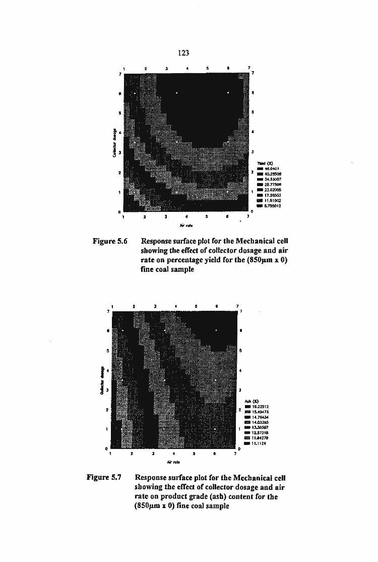
1 7

• 5

14 I J

2

0 1

Figure 5.6

I

i5

14 IJ

2

Figure 5.7

123

2 J 4 5 ll

Yield(%) -411.0401

2 - 40.2e5011 .34.53007 • u .n5011

1 -23.02005 -17.26503 -11.51002 - 5.75!5012

2 l .. 5 ll

Nrrate

Response surface plot for the Mechanical cell showing the effect of collector dosage and air rate on percentage yield for the (850p.m x 0) fine coal sample

• i5

4

;s

Mil(%) -16.22512

2 m15.4g.u3 -14.76434 814.0JJ~

-1~7

-12.57JIIl 1112111U4279 -11.1124

Response surface plot for the Mechanical cell showing the effect of collector dosage and air rate on product grade (ash) content for the (850p.m x 0) fine coal sample

124

14 14

12 12

10 10

~ c: 8 8 0

I 8 8 Ylold (~

-50.05521

- 43.711331 -37.54141

- 31 .284!11 4 4

- 2!1.027&1 -18.77071 B!112.S138 • 6.zssgoz

Froth.- dosage

Figure 5.8 Response surface plot for the Mechanical cell showing

Figure 5.9

the effect offrother dosage and flotation time on percentage yield for the (850J1m x 0) fine coal sample

II

8 Ash (") .,8 -17 -16 1111111 15

4 .,4 atJ ll:!.al2 .,1

2 45

Frothar do•age

Response surface plot for the Mechanical cell showing the effect of frother dosage and flotation time on product grade (ash) content for the (850J1m x 0) fine coal sample

125

TABLE 5.6 : PROCESS CONDITIONS NECESSARY TO OBTAIN OPTIMUM PERFORMANCE FOR THE MECHANICAL BATCH CELL TREATING (850J.lm X 0) TWISTDRAAI FINE COAL

Yield Middle-High Air rate ( Q/min) Middle-High (3 .5 - 6.0) Frother dosage (ppm) High (40) Collector dosage (Q/t) Middle-High (3 .5- 6.0) Flotation time (min) Low-Middle (3.0- 7.5)

Ash Low-Middle Air rate (Q/min) Low-Middle (1.5- 3.5) Frother dosage (ppm) Low-Middle (20 - 30) Collector dosage (Q/t) Low-Middle (1.0- 3.5) Flotation time (min) Low-Middle (3.0- 7.5)

From the results in Table 5.6 it can be seen that the best compromise would be to use settings in the middle ofthe factorial programme for both air rate (3 .5 1/min), collector dosage (3 .5 1/ton) and frother dosage (30 ppm). Flotation time should be as short as possible (between 3 and 7.5 minutes according to the experimental design programme used) .

From the detailed Mechanical cell test results shown in Tables D4.1 to D4.4, tests 1, 10, 14, 18 and 20 correspond to the optimum parameter conditions argued statistically. These tests yielded mass recoveries respectively of: 39.7%, 41.3%, 38.9%, 31.9% and 37.8% for tests 1, 10, 14, 18 and 20. The concentrate ash obtained for these tests were respectively: 13 .3%, 14.0%, 13 .9%, 14.8% and 13 .6%.

From the single-stage flotation investigation, Test 1 (39.7% yield and product ash of 13 .3% was considered optimal (highest yield at ca 13% ash) and would be used in a subsequent cleaner flotation investigation in order to ascertain whether cleaning would reduce the ash content to below 10%.

In addition, regression analysis was used to produce models describing the relationship between the dependent and independent variables for the mechanical cell. These models are presented in Table A3 .3 in the appendix, which includes the correlation co-efficient for both dependent variable (yield and ash). Plots between the observed and model-predicted values are shown in Figures 5.10 and 5 .11 . The correlation co-efficients obtained range between 81% and 95% indicating a relatively high degree offit ofthese models.

126

60 r---------------------~------~------~1 ----~~ I I I

I I I I I • ------- -~--- ----~------- -~--------~-----~- --------

1 I I I t tl I I I I I

50 I I I I I I I I I I I I I I I

---- ----~ -------~- -------~-------- --------~--------1 I I t I t I

: : : . : : 40

: : . : : : --------~-------~---- ---- ------- -~------ --~----- - --

1 I I I I

: : . : : : I I t I I I I I I I I

20 --------L------- ------ -- ~--------~--------~--------: . : : : : I I I I I I I I I I I t I I I I

-------~-- --- ---~----- - --~--------~--- - ----1 I I I 10 I I I I I I I I I I I I I I I I

o~~--~--~--~--~--~~--~--~--~--~~

0 1 0 20 30 40 50 60 predicted

Figure 5.10 Plot of predicted vs observed results with respect to percentage yield for the Mechanical cell when treating (850p.m x 0) Twistdraai fine coal

18~--------.---------.---------.-------~

16

12

10 10

I I I I I I I

I I I ------------, - ------------r-- ---------- -------------1 I I I I t I

: : . : I I t I I I I

I ' + I I t I I ____________ , _______________ . ______ ___ , ________ ____ _

I I tl I

t tl I I I I I I I I I I I

-------------~------------~-- - ----------1 I ' I I I I

t I I t I I

I I t I I

12

I I

14 predicted

16 18

Figure 5.11 Plot of predicted vs observed results with respect to product grade (ash) content for the Mechanical cell when treating (850p.m x 0) Twistdraai fine coal

127

5.3.1.2 Microcel column flotation results

5.3.1.2.1 Global flotation results

Single-stage Microcel column flotation tests were conducted on the Twistdraai fine coal sample (850 11m x 0) described earlier in section 3 .2.1.2 of this thesis. Characterisation data for this sample is given in section 5.2. As stated in section 5.2.6.1, only collector (K) (1 - 6 Q/t) and heavy alcohol frother (20 - 40 ppm) will be used as reagents in the single­stage test programme.

A total of31 column flotation tests were conducted. Experimental methods and range of operating conditions investigated can be found in section 3.6.2.2 ofthis thesis. Details of each individual run, and the results obtained, are given in Tables D5 .1 to D5.8 in the Appendix D5.

30

~ 25 .P - - - - - - - - - - - - - - - - - - - - - - - - - . - - - - - . - - - - - - . - - - . - - - - - - -.- -J'- - - .- - - - - - - -

:I: ft (/) 20 <{

1- 15 u :::> 0 10 0 a: a. 5

- - - - . - - . - - - - - - - - . - - - - - - - - - . -A- - . - - - - - - . - - - -A. - -~ - - - - - - - . - - - - - - -

----- ---.. .- .... -_ .. _ .. _-"':.:- ...... _t:,;.-/!t-< --- --_----- -- -- ------ • •- • • • • A ··"-'~-~- ~--~- -:'-_:=_:-.;_ -:-_--::-~ • • •--- -- •-- •-•- •- ---- --• • •-- -- ------__ er---- - Go'"--::"'- • - - - - - - • • - - . - - . - .. - - - - - • . - - - - - - . - - - - - - - --- - -- - - - - • - - - - - - -

0 0 20 40 60 80 100

PRODUCT YIELD(%)

MICROCE.l COLUMN WA~~~.ITY RELiASE

Figure 5.12 The separation performance achieved by the Microcel column cell, the release curve and washability for the (850,.._m x 0) fine coal sample

The global results obtained for the Microcel column in terms of product yield and ash are graphically depicted in Figure 5 .12, together with coal washability and release float analysis.It can be observed from Figure 5.12 together with Tables D5 .1 to D5.8 that the lowest product ash achieved in the column flotation testwork was 13 .0% at a yield of 36.7% (Test 17), and the highest yield obtained was 75 .2% at a product ash of 16.5% (Test 7).

In general, most tests were clustered reasonably close to the theoretical release curve.

128

5.3.1.2.2 Parameter effects

Multiple regression analysis was conducted on the data generated from the 31 Microcel column flotation cell tests, and the results can be observed in Tables A3.4 and A3.5 given in Appendix A3 . The two dependent variables tested were mass (yield %) and ash content.

From the results given in Tables A3.4 and A3 .5, the t-value statistic again should be used in order to identifY the most significant operating parameter for each dependent variable. (The t-value closest to zero signifies the most significant parameter).

In the case of mass % yield, the air rate*frother dosage interaction; feed rate; as well as collector*wash water rate interaction and frother*wash water rate interaction were all significant, with the air rate*air rate quadratic term least significant. Likewise, in the case ofthe product% ash, the wash water rate and collector*wash water interaction was the most significant parameter and the collector*air rate least significant.

It can be observed in Figure 5.13, that air rates between 4 - 5.5 l/min, as well as high frother dosage (i.e.400 g/t), result in a high yield. This can be explained by the fact that the higher the air rate, the more bubbles are available within the ·cell thereby improving the probability of collection. Increases in flotation yield and recovery arising from changes in these operating parameters can be attributed to :

(i) Improved pulp phase flotation kinetics. (ii) Higher solids loading of the froth bubble bed, i.e. froth phase kinetics

At steady state, the rate of particle collection by bubbles in the pulp phase and the rate of solids reflux in the concentrate are equal. One of these transport steps are usually rate limiting: consequently, changes in operating parameters will predominately affect the kinetics of the rate limiting phase.

As can be observed from Figure 5.14, high frother dosage together with high air rate also yield undesirably high ash. This basically indicates that selectivity is impaired and recovery by entrainment features strongly under these conditions.

High yields are also obtained when using feed rates of 0. 9-1 .5 l/min, and low wash water rates (0.45-0.60 1/min) or, low feed rates (0.6-0.9 1/min) and high wash water rates >0. 75 I/ min. (See the response curve in Figure 5 .15). This curvature can perhaps be explained by the fact that at high feed rates, (i.e. reducing the residence time), the column was not operating under carrying capacity limitations. Under these conditions, low wash water rates resulted in the froth phase not being very well mixed and reflux or dropback was limited. In the case oflow feed rates (i.e. increased residence time), the column operated under rate control and high wash water rates stabilised the froth zone thereby reducing coalescence.

This same trend can also be observed from Figure 5. 16, where high ash was also obtained for the feed rate*wash water rate interaction. This again can possibly be explained by the fact that selectivity is impaired at low wash water rates as the entrainment mechanism predominates under these conditions.

~

3.5 150

250

200 250

129

JOO 350

JOO 350

Frothar dooaga

450 6.5

6

5.5

5

4.5

~

3.5 450

Yoald (X)

- 59.990H 11!88 55.8173

- 51 .64+~ 11!!811 +7.+7162

- -43.2!1878 -39.12594 FA 34.9531

-30.78026

Figure 5.13 Response surface plot for the Microcel column showing the effect of frother dosage and airrate on percentage yield for *h"' (jll:\O"m X 0\ fin"' enol S"mp'"' -. •'-' _ _. ,... J •••'-' '"'"• Ua • a"'

200 250 300 350

200 250 300

Frothcr doscga

450 6.5

6

5.5

5

~.5

~

J .5 450

Alh (r.) - 17.67332 m 11.2nos

- 16.88084 11!!811115.-4846 -16.08835

- 15.59211 1111111 15.29587

- H .8996J

Figure 5.14 Response surface plot for the Microcel column showing the effect of frother dosage and airrate on product grade (ash) content for the (850J.1m x 0) fine coal sample

.45 1.6

1.4

1.2

.8

.6 .45

.5 .55

.5 .55

130

.6 .65 .7

.e .65 .7

Wash wotor rate

,75 .8

.75 .8

1.4

1.2

Yield (%)

- 57.402.27 1111111 52.96327 - 48.!52428

.8 111111 44.08528

.6 .85

-39.64629 -35.20729 11Z1 30.7 683

- 215.J29J

Figure 5.15 Response surface plot for the Microcel column showing the effect of wash water rate and feed rate on percentage yield for the (850Jlm x 0) fine coal sample

.45 .5 .55 .6 .65 .7

1.2

.5 .55 .6 .65 .7

Wash woll!r roll!

.75 .8

.7S .8 ·'"

1.4

1.2

Ash (ll:) -19.09442 llll!ill 18.27283

- 17.45123 .8 llR8 16.62963

- 15.80804 - 14.986« 11l.i'5114.1f!.485

-13.34325 .6

Figure 5.16 Response surface plot for the Microcel column showing the effect of wash water rate and feed rate on product grade (ash) content for the (850f.1mx 0) fine coal sample

131

However, the high frother dosages used in this investigation (based on visual observation of the froth phase under high wash water rates), produced a froth which appeared very stable and which inhibited the overflow of the concentrate and periodic (manual) removal of this froth "plug" was required. An additional problem in attempting to explain this interaction effect is the fact that coarse coal particles <850J.lm were used in a counter­current open column where the force of gravity was competing with surface forces, i.e. good quality low-ash coal may be rejected into the tailings purely on the basis of particulate density and . finer particles were preferentially recovered in the flotation concentrate.

From the literature (Finch, 1990), it is clear that the addition of wash water is a critical parameter in the operation of the column cell, and an optimum rate exists. At low wash water rates, a negative bias exists in the column (i .e. there is a net upward flow of water), resulting in poor concentrate grades, and at excessively high wash water rates, valuable particles are "washed" from the bubble surface, resulting in poor recoveries. The absolute wash water rate is, however, of secondary importance; it is the bias rate (i.e. net downward slurry flow rate) which determines the grade of the product.

The effect of superficial bias rate on column cell concentrate ash content can be observed in Figure 5.17. It may be observed from this figure that an increase in the bias rate generally resulted in an improvement in the concentrate grade, i.e. a decrease in the ash content (the overall trend is indicated by the linear regression line plotted in Figure 5.17.

30r--------------------------,

~ 20 :I: en <

-- -- ·-o · ----o·- -·- · ·- -·-·· · -··· · ·· ·· · ··

·w o ~ 15 a: 1- l!jl z w u ~ 10 ·- - · · - -- - · - ···---···--- ·· ----·--· - ------u

0~--~----~----~----~--~ 0 0.2 0.4 0 .6 O.B

BIAS RATE (cm/s)

Figure 5.17 Effect of superficial bias rate on the Microcel column product ash content

132

From all ofthe surface response plots given in Figures 5.13 to 5.16 it is clear that high yields are generally associated with high ash, and a compromise is again required in order to obtain the optimum performance. Table 5.7 summarises process conditions necessary to obtain the best compromise. An understanding of the terms "low", "middle" and "high" can be obtained from the factorial design test programme given in Table A2.2 in Appendix A2.

TABLE 5.7 : PROCESS CONDITIONS NECESSARY TO OBTAIN OP~PERFORMANCEFORTHENITCROCELCOLUMN

TREATING (850J1m X 0) TWISTDRAAI FINE COAL

Yield Middle-High Air rate (e/min) Middle (50) Froth depth (em) All (35- 55) Collector dosage (Q/t) Middle-High (3.5- 6.0) Feed rate (Nmin) Low-Middle (0.75- 1.13) Washwater rate (Q/min) All (0.5 - 0.8) Froth dosage (g/t) Middle-High (300 - 400)

Ash Low-Middle Air rate (Q/min) All (4.0- 6.0) Froth depth (em) All (35- 55) Collector dosage (Q/t) Low-Middle (1.0- 3.5) Feed rate (Q/min) Low-Middle (0.75- 1.13) Washwater rate (Q/m.in) Low, High (0.5 and 0.8) Froth dosage (g/t) Low-Middle (200 - 300)

From the results presented in Table 5.7, the best compromise would be to use settings in the middle of the factorial programme for both air rate (5 1/min), collector dosage (3.5 1/ton) and frother dosage (300 g/t). Feed rate should fall between 0. 75 - 1.13 1/min, while, the washwater rate should be either 0.5 or 0.8 1/min and the froth depth can range anywhere between 35 and 55 em.

From the detailed test results shown in Tables D5.1 to D5.8, Tests 2, 17, 22, and 29 produced concentrates containing< 14% ash. The actual yields produced for these tests are respectively: 15.7%, 36.7%, 38.9% and 34.3%. The best result obtained is test 17 (i.e. 36.68% yield at 13.0% ash). The parameter settings for this test are however not in agreement with the statistical argument given above. (i.e. air rate (6 1/min), collector dosage (1 1/ton) and frother dosage (200 g/t). The feed rate setting was 1.5 1/min, while the washwater rate was 0.8 1/min and the froth depth 55 em.

It can be concluded that the curvature evident from the surface response models obtained for the Microcel column could not be used to satisfactorily describe the optimum region for the Microcel column cell.

From the single-stage flotation investigation, Test 17 (36. 7% yield and product ash of 13.0%) was considered the best result (highest yield at 13% ash), but would not be used in a subsequent cleaner flotation investigation, since false conclusions could be obtained which would negatively impact on the cell efficiency comparison.

/

133

In support ofthe conclusion above, regression analysis was also used to produce models describing the relationship between the dependent and independent variables for the colurim cell. These models are presented in Table A3.6 given in Appendix A3, which includes the correlation co-efficient for the two dependent variables. Plots between the observed and model-predicted values are shown in Figures 5.18 and 5.19. It is clear that the correlation· co-efficients obtained here range between 67% and 84% indicating a relatively low degree of fit.

5.3.1.3 Single-stage Jameson cell flotation results

5.3.1.3.1 Global results

Single-stage Jameson cell flotation tests were conducted on the Twistdraai fine coal ( <850Jim x 0) size fraction described earlier in section 3.2.1.2 of this thesis. Characterisation data for this sample is given in section 5.2.

As stated in section 5.2.6.1, only collector (K) (1 - 6 Q/t) and heavy alcohol (200- 400 g/t) frother will be used as frother in the single-stage test programme.

A total of 31 Jameson cell flotation tests were conducted. Experimental methods and range of operating conditions investigated can be found in section 3.6.3 of this thesis. Details of each individual run, and the results obtained, are given in Tables D6.1 to D6. 7 in Appendix D6.

The global Jameson cell froth flotation results. in terms of product yield and ash are graphically depicted in Figure 5.20, together with coal. washability and release float analysis.

It may be observed from the data in Tables D6.1 to D6. 7 together with Figure 5.20 that the lowest product ash achieved in the Jameson cell testwork was 13.1% at a yield of 46.4% (Test 12), and the highest yield obtained was 83.5% at a product ash of22.6% · (Test 18). In general, most tests were clustered in the vicinity ofthe theoretical release curve.

134

80~------~--------~--------~--------~

60

20

I I I I I I

I I I I I I ------------""1-------------r------------·-- -·-----------1 I + I I I + I I I I I I I I +I I

: . : : I I I

------------;------~---- - ____________ , ____________ _ I I I I I I I I I

: . : . : I I I I I I

+I I I ------------ ----~-------~------------~-------------1 I I +I I I

I I I I I I I I I I I I I I I I I I

o~~~--~~--~~~--~~~--~~~--~~~

0 20 40 predicted

60 80

Figure 5.18 Plot of predicted vs observed results with respect to percentage yield for the Microcel column when treating 850p.m x 0 Twistdraai fine coal

20~--------~--------~--------~------~

18

14

I I I I I I I

I I I I I

+ I I I

•

------------""1-------------r------------ -------------1 I + I I I I I I I I I I : .: : . I I I I I + I

------------;----~------- ------------;-.-----------. I I + +I , I

I I I I I I I I I I

+ I I -------------~------------~-------------t : .

I I I I I I

12 ~--~----~--~----~--~----~----~--~ 12 14 16

predicted 18 20

Figure 5.19 Plot of predicted vs observed results with respect to product grade (ash) content for the Microcel column when treating 850p.m x 0 Twistdraai fine coal

30 -~ 25 :I: CJ) 20 <(

t- 15 u :::> 0 10 0 a: a.. 5

0 0

135

... ----- ~ -- .. -- ---- ----- .... -.... -- .... ------- -;- .. -- ..... - .. --- .. -- .. -- .. --------p

- ---- - ---.- --- ---- ---- -.- ------------ - -------------- --/- - - -- - -----.. ~. -------------.- ----------------------,- .- ----:Jiill· -·- -----------. . ............ . --. ----- -- - ------ --- - ---------- --.... '- -- - - - ------------ -- ------. . . ~ .... ----- - .. .. .. .. .. - - - .. :..;. ...-~ ~- -.... - - - - .. -- ... --- .. --- - - - - --.. - -- ..... - - - .. - - -

~-­----- - b-r-~- - - - - - - - - - - - - -- - -- - - - - - - - - - - - - - - - - - - - -- - - -- - - - - - - - -- - - - • - -

20 40 60 80 100 PRODUCT YIELD(%)

JAMESON CELL WASHABILITY RELEASE • --b-- 0

Figure 5.20 The separation performance achieved by the Jameson cell, the release curve and washability for the (850J1m x 0) fine coal sample

5.3.1.3.2 Parameter effects

Multiple regression analysis was conducted on the data generated from the 31 Jameson cell tests, and the results can be obseiVed in Tables A3.7 and A3.8 given in Appendix A3. The two dependent variables tested were mass (yield %) and product ash content.

From the results presented in Tables A3.7 and A3.8, the t-value statistic again should be used in order to identify the most significant operating parameter for each dependent variable. (The t-value closes to zero signifies the most significant parameter).

In the case of mass(% yield), the froth depth*air rate interaction as well as the quadratic froth depth*froth depth term were equally the most significant, and the collector* collector quadratic term was least significant. Likewise, in the case.ofthe product% ash, the froth depth *froth depth quadratic term as well as the feed pressure*air rate interaction were equally the most significant, while, the feed pressure*collector dosage interaction was least significant. From the above it can be concluded that these variables will provide the most useful predictive information, and quadratic terms were included because a quadratic trend could be obseiVed in the data.

It can be also be obseiVed from the response surface plot given in Figure 5.21, that both shallow froth depths (15-35 em) as well as high air rates (>6 l/min) result in high yield. This can be explained by the fact that the higher the air rate, the more bubbles are available within the cell thereby improving the probability of collection. The shallow froth depth in essence also provides a larger collection zone, hence, less reflux or drop-back can be expected in the shallower froth zone than in a deeper froth zone.

136

Fortunately, as can be observed from Figure 5.22, high air rate together with a deep froth do not yield undesirably high ash. This indicates that selectivity is not negatively affected under these conditions, and air rates between 4 and 8 I/ min can be used, provided a froth depth of 0.5 m is maintained, i.e. it is possible to obtain yields in excess of 32% when using air rates above 6.5 1/min whilst maintaining product ash at c.a. 13% provided a froth depth of0.5 m is maintained.

High yields (c.a. 75%) are also obtained when using feed pressures exceeding 130 kpa and air rates above 5 1/min (Figure 5.23). Conversely, yield is significantly reduced (c.a.< 26%) when using feed pressures of 110 kpa and air rates below 4 I/ min.

This same trend can also be observed from Figure 5.24, where high ash was also obtained for the feed-pressure*air rate interaction. The feed pressure determines the volumetric flowrate to the cell, and air rate being naturally induced (but linearly correlated to the amount offrother present in the pulp), constitutes a strong drive towards mass recovery. As a result, poor selectivity is obtained as shown by the negative influence on product ash content.

From Figures 5.23 and 5.24 it is clear that high yields are generally associated with high ash, and a compromise is again required in order to obtain optimum performance. Table 5.8 summarises process conditions necessary to obtain the best compromise.

TABLE 5.8: PROCESS CONDITIONS NECESSARY TO OBTAIN OPTIM:Ul\1 PERFORMANCE FOR THE JAMESON CELL TREATING (850J.1m X 0) TWISTDRAAI FINE COAL

Yield Middle-High Air rate (Q/min) Middle-High (6.0- 8.0) Froth depth (em) Low-Middle (15 .0- 32.5) Collector dosage (Q/min) Middle-High (3.5- 6.0) Feed pressure (Kpa) Middle-High (135- 165) Washwater rate (Q/min) Low-Middle (0.95 - 1.20) Froth dosage (g/t) Middle-High (300- 400)

Ash Low-Middle Air rate (Q/min) Low-Middle (4.0- 6.0) Froth depth (em) Middle-High (32.5- 50.0) Collector dosage (Q/min) Low-Middle (1.0- 3.5) Feed pressure (Kpa) Low-Middle (110- 135) Washwater rate (Q/min) Middle-High (1.20- 1.45) Froth dosage (g/t) Low-Middle (200 - 300)

8

7

5

4

137

15 20 25 30 35 4C 45 50 55

15 20 25 30 35 40 45 50

f'roth depth

9

8

7

6

5 Yield (X) -83.02222 lliZl 74.64355

- 66.264~ lllll:l 57.88623

4 -49.50756 IIIII 41 .1289 D 32.75024

- 2<4.37158

Figure 5.21 Response surface plot for the Jameson cell showing the effect of froth depth and feed rate on percentage yield for the (850J.!m x 0) fine coal sample

15 20 25 30 35 40 45 50

10 15 20 25 30 35 40 45 50

f roth depth

8

7

6

5 Ash (,;) -22.4975 m 21 .2323 -19.96709 111!!118.70189

4 -17.43669 - 16.17149 rt:iJ H.90629 -13.64109

Figure 5.22 Response surface plot for the Jameson cell showing the effect of froth depth and feed rate on product grade (ash) content for the (850p.m x 0) fine coal sample

100 110

110

Table 5.23

110

138

120 130 140

120 130 140

Feed pru•ur•

150 160

150 160

5 Yield (X) -74.65235

- 66.620J2

- !58.58828 111111 50.55624

4 -42.5242 -34.49216 -26.46012 -18.42808

Response surface plot for the Jameson cell showing the effect of feed pressure and airrate on percentage yield for the (850J.1m x 0) fine coal sample

120 130 150 ISO

8

7

6

5 A:!lh (1.:) - 19.26144 118!1 18.35376 -17.-4--4008 182:1 16.5384

4 - 15.63072 -14.72304 IIE8I 13.8 I 538

-12.90768

110 120 130 140 150 160

Figure5.24

Feed pressure

Response surface plot for the Jameson cell showing the effect of feed pressure and airrate on product grade (ash) content for the (850J.lm x 0) fine coal sample

139

An understanding of the terms "low", "middle" and "high" can be obtained from the factorial design test programme given in Table A2.3 in Appendix A2.

From the results presented in Table 5.8 it can be observed that the best compromise for low ash would be to use settings for air rate (4 - 6 1/min), froth depth (32.5 -50 em), collector dosage (1- 3 1/ton), frother dosage (200 -400 g/t), feed pressure (110 -135 kpa) and washwater rate (1.2 -1.451/min).

From the detailed test results shown in Tables D6.1 to D6. 7, Tests 3, 6, 12, and 24 produced concentrates containing< 14% ash. The actual yields produced for these tests are respectively: 27.1 %, 27.0%, 46.4% and 18.5%. The best result obtained is undoubtedly test 12 (i.e. 46.4% yield at 13 .1% ash).

The parameter settings for this test require settings for air rate (41/min), froth depth (50 em), collector dosage (6 1/ton), frother dosage (400 ppm), feed pressure (110 kpa) and washwater rate (1.45 1/min). It is only in the case of collector and frother requirements that disagreement between this test and the model predictions are observed.

From the single-stage flotation investigation, Test 12 (46.4% yield and product ash of 13 .1% was considered optimal and will be used in a subsequent cleaner flotation investigation.

Regression analysis was also used to produce models describing the relationship between the dependent and independent variables for the Jameson cell. These models are presented in Table A3 .9 given in Appendix A3, which includes the correlation co-efficient for both dependent variables. Plots between the observed and model-predicted values are shown in Figures 5.25 and 5.26. The correlation co-efficients obtained here range between 72% and 86% indicating a reasonable degree of fit.

5.3.1.4 Single-stage froth flotation cell comparison (850J1m x 0 coal)

5.3.1.4.1 Global comparison

The global results obtained in terms of product yield and ash content for the Mechanical cell, Microcel column and Jameson cell when treating the (850Jlm x 0) Twistdraai fine coal sample are graphically <lepicted in Figure 5.27, together with coal washability and the release float curve.

The results from Figure 5.27 indicate that each of the flotation devices tested were capable of beneficiating the Twistdraai < 850Jlm x 0 coal fraction to ash levels c.a. 13% in a single-step operation.

The best result (i.e. the highest yield at an ash content ofc.a. 13%) achieved in each ofthe different cells is presented in Table 5.9.

] <ll .g

140

100 ~----------------~--------------1 ------~

80

60

40

20

I I I I

I I I I •

----------~--~-------~---------~~----j-____ 1 ----------1 I I • ••

: : :• •• I I I I t I

: : I t : ----------L-----~----L--------- ----------L----------1 I I

: . : : I I I

: . : : I I I I

----------~---------- ----------~---~------~----------1 I I I I I I I I I I I I I I I I t • I I I I I I I I I I I ------~---r----------r----------r----------

1 I I I I I I I I . : : : I I I

0 ~--~--~--~--~--~--~--~----~--~~ 0 20 40 ed" ted 60 80 100 pr IC

Figure 5.25 Plot of predicted vs observed results with respect to percentage yield for the Jameson cell when treating (850J.lm x 0) Twistdraai fine coal

24~---------------------------~------------~

22

I I I t I

I I I It --------T--------,---------r--------,--------1 I I I I I I I I I I I I I I I I

"'d 20 ~

--------~--------~---------~------~-~---------~--------1 I I •• tl I I I I • I I I I I I I

<ll I I I I I

.g 18 I I I I I

--------~--------~--------- --------~---------~--------1 I I I I. I I I I I

: :•. : : : I I I I I I • I I I --------T-------- ---------r--------,---------r--------16 1 I I I I I I I I I I I I I I I I I I I I I I I I -------~---------r--------~---------r--------

1 I I I 14

I I I I I I I I I I I I I I I I

12~~--~--~~~~--~--~~--~--~~--~

12 14 16 18 observed

20 22 24

Figure 5.26 Plot of predicted vs observed results with respect to product grade (ash) content for the Jameson cell when treating (850J.1m x 0) Twistdraai fine coal

30

?fl. 25

:I: (J) 20 <(

t> 15 ::::> 0 0 10 a: a.. 5

141

OL---------~--------~------~~------~----~--~ 0 20 40 .60 80

PRODUCT YIELD(%)

MECHAN:;AL CELL MICROCEl_ COLUMN JAMES_&N CELL WASHABILITY ~~~:~,:;.:

Figure 5.27 Comparison between the single-stage separation performance achieved by the three flotation cells, the release curve and washability when treating (850p.m x 0) Twistdraai fine coal

100

TABLE 5.9 : THE OPTIMUM RESULT OBTAINED FOR THE THREE FLOTATION CELLS DURING SINGLE-STAGE OPERATION WHEN TREATING (850p.m X 0) TWISTDRAAI FINE COAL

CELL TYPE YIELD ASH CONTENT COLLECTOR FROTHER (%) (%) DOSAGE (Ut) DOSAGE

(g/t)

Mechanical 39.7 13.3 3.5 300 Microcel 36.7 13.0 1.0 200 Jameson 46.4 13.1 6.0 400

From the results given in Table 5.9 it can be observed that the optimum performance of each of the three devices tested were comparable, and that the Jameson cell yielded higher mass % recovery at similar ash levels when compared to the other cells.

However, the Microcel column had the lowest collector requirement and the Jameson cell the highest reagent requirement. This increased reagent requirement for the Jameson cell, (albeit at increased yield), in comparison to that required by the other two cells could represent a significant negative factor with respect to the use of this unit in the Twistdraai circuit.

142

It is also evident from the global results discussed in sections 5.3.1.1.1, 5.3.1.2.1 and 5.3J .3.1 for the Mechanical cell, Microcel column and Jameson cell respectively that the yield/ash plots achieved for the leeds Mechanical cell were less scattered than those achieved in either the column or Jameson cells. These differences may be attributed to differences in the sensitivities of the different technologies to variations in their operating conditions. Alternatively, they may simply be a result of the operating regimes of the more recent technologies being less defined.

The latter reason was compounded by the fact that no established flotation procedure for the Twistdraai < 850f.!m X 0 fine coal has been developed thus far, and the operating range selected for this investigation was fairly wide in order to ensure some results (at optimal conditions) would be obtained.

The throughput capacity and superficial velocity data obtained for the two continuous cells can be observed in Table 5.10.

TABLE 5.10: THROUGHPUT CAPACITY AND SUPERFICIAL VELOCITY RESULTS OBTAINED FOR THE 2 CONTINUOUS CELLS WHEN TREATING (850Jtm X 0) TWISTDRAAI FINE COAL

CELL FEED GAS WASHWATER THROUGH- COMBUST. TYPE RATE RATE RATE (cm/s) PUT RECOVERY

(cm/s) (cm/s) (tlhr.m1) (%)

Microcel 0.82 3.26 0.43 1.42 44.7 Jameson 1.59 0.82 0.30 1.51 55.8

As shown in Table 5.1 0, it was found that the combustible recovery for the Jameson cell was 11% higher than that obtained by the Microcel column and the throughput capacity was also higher for this cell by 0.09 tlhr.m2

. A further advantage of the Jameson cell is that it required 4 times less air and 1. 4 times less wash water than the Microcel column whilst recovering 11% more combustibles.

From the data presented earlier in Table 5.9 the Jameson cell had the highest reagent requirement. However, the other advantages obtained with the Jameson cell when compared to the Microcel column given in Table 5.10, i.e. high throughput, low air and wash water requirement must also be taken into account when identifying the best flotation cell for treatment of the Twisdraai < 850f.!m x 0 fine coal fraction.

5.3.2 Single-stage test results for the deslimed (300J1m x 38Jtm) fine coal sample

Coal characterisation for the deslimed (300f.!m x 38f..lm) fine coal sample consisted of size, ash-by-size, release flotation analysis and preliminary reagent screening. These results were presented in section 5.2.

For the composite (850f.!m x 0) fine coal sample the Jameson flotation cell was shown in section 5.3.1.4.1 to yield an 11% increase in combustible recovery at similar product ash

143

when compared to the Microcel column during single-stage testing, but at higher reagent dosage. Surface characterisation results reported in section 5.3 of this thesis also clearly indicate that the ultrafine <38J.1m slimes fraction appeared detrimental to the froth flotation process since it contains significantly higher carboxylic acid functional groups and is more oxidised than the coarser +38J.1m coal fraction. Floatability of the <38J.1m fraction was shown to be poor in section 5.3.2.2 above. However, with the removal ofthe <38J.1m fraction, and the reduction in top size to 300J.1m, a much lower collector consumption would be expected with respect to the use of the Jameson cell.

5.3.2.1 Global results

A total of 20 Jameson cell flotation tests were conducted using collector (K) at a fixed concentration of 1 1/t for all tests. Experimental methods and range of operating conditions investigated can be found in section 3.6.3. Details of each individual run, and the results obtained, are given in Tables 06.8 to 06.11 in Appendix D6. The global results in terms of product yield and ash are graphically depicted in Figure 5.28, together with the coal release float analysis. ·

35.-----------------------------------~

30 -----------------------------------------------. ~ ~25 ------------------------------------------til tU

• • 10 ----~.--~~·~-~~-dt-~-~-~-~-~-----------------------

•

10 20

Figure 5.28

30 40 50 60 70 80 90 100 Product yield (%)

Release analysis results compared with single-stage Jameson cell flotation results when treating the deslimed (300f.1m x 38f.1m) Twistdraai fine coal sample

It can be observed in Figure 5.28 together with Tables 06.8 to 06.11 that the lowest product ash achieved in the Jameson cell testwork was 7.8% at a yield of only 3:4% (Test 15), and the highest yield obtained was 60.5% at a product ash of 12.5% (Test 16). In general, most tests were clustered reasonably close to the theoretical release curve. Test 2 yielded the highest mass recovery of22.5% at the desired ash content of 10.0% in only

144

a single-flotation step requiring a collector usage of only 1 Vt. Clearly, froth flotation of the Twistdraai <300J1m x 38J1m fraction renders a possible solution to maximising combustible recovery for the fine coal circuit.

5~3.3 Two-stage flotation test results for the (850J.lm x 0) fine coal sample

The motivation behind conducting two-stage flotation was to ascertain whether the ash content could be further reduced when using the optimum single-stage settings for both the leeds Mechanical cell and Jameson cell. Furthermore, ash-by-size conducted on the cleaner flotation products would indicate if differences in preferential size class recovery was occurring with these two flotation devices. In addition, efficiency testing would also be conducted using the samples and data generated from the two-step flotation testwork in order to describe froth flotation in terms of the ecart probable ( epm) for both the Mechanical and Jameson cells.

5.3.3.1 Global results

The operating conditions used in the two-stage flotation tests are given in Tables D7.1 and D7.2 in Appendix D.

The results obtained in terms of product yield and ash content for both the Mechanical leeds cell and Jameson cell cleaner flotation tests are graphically depicted in Figure 5.29, together with coal washability and release float analysis.

30r.=======================,-------, Washability Release Mechanical Jameson

- -+-- --e-- --25

cell cell

,.-..

~ '-" 20 ~ ro t) 15 .g 0

,:i: 10

5 --- --------------------------------------------------

20 40 60 80 100

Product yield (%)

Figure 5.29 The effect of two-stage flotation for the Mechanical cell and Jameson . cell the release curve and washability when treating (850J.1m x 0) Twistdraai fine coal

145

It can be observed from Figure 5.29 that the final cleaner concentrate ash achieved in the Jameson cell testwork was 11.5% at a yield of 82.7%. This result was obtained from a rougher concentrate feeding the cleaner stage containing 13.1% ash. This further ash reduction of 1.6% obtained in the cleaner stage resulted in a subsequent loss in yield of 8.0%. This reduces the overall mass% yield to 38.3% containing 11.5% ash.

In the case of the Mechanical leeds cell, the final cleaner concentrate ash achieved was 12.2% at a yield of73.8%. This result was obtained from a rougher concentrate feeding the cleaner stage containing 13.3% ash. This further ash reduction of 1.1% obtained in the cleaner stage resulted in a subsequent loss in yield of 10.4%. This reduces the overall mass% yield to 29.3% containing 12.2% ash. Clearly, both flotation cell curves follow the slope of the release curve, but the Jameson cell is always marginally superior indicating a more efficient separation.

5.3.3.2 Cleaner concentrate fractional yield-by-size and ash-by-size results

A comparison between the fractional concentrate yield data obtained for both the Mechanical and Jameson cells is given in Figure 5.30. In this case, the fractional yield by size figures obtained from the flotation testwork were corrected by adjusting them in accordance with their overall contribution to the final cleaner concentrate in terms of mass % recovery. In this way, it is possible to observe from a fractional viewpoint, the amount of material recovered in each size fraction in accordance with what was present in the original feed.

It can be observed from Figure 5.30 that the original feed or head sample contains mainly coarse +500Jlm and ultrafine -38Jlm coal.

The trends shown by the flotation devices indicate that no coarse +SOOJ.!m coal was recovered by either cell, but that the Jameson cell always recovered more -300+38flm coal than did the leeds Mechanical cell. Experimental error is likely in the +75Jlm and +38Jlm fractions for the Jameson cell, where slightly more of this fraction is present in the concentrate than was originally present in the feed.

A comparison between the fractional concentrate ash contents obtained for both the Mechanical and Jameson cells are plotted in Figure 5 .31.

It can be observed from Figure 5.31 that significant fractional ash reduction was obtained for both cells when compared to the fractional ash present in the feed.

The trends shown by the flotation devices indicate that fractional concentrate ash generally increases with a decrease in particle size.

·...t 0

... 0·

146

~ ~------------------~----------------------------~

25

~20 ~

~ •f>. 15 0 ::S·

"'0 0 ~ 10

5

Head Jameson Leeds cell . cleaner cone cleaner cone.

-----------~~---~------,,,---r---------- -

0 ~-=--~----~----~----~----~----~------~----~ +500 ' +300 + 212 + 150 + 106 + 75

Particle size (f.lm) +45 +38 -38

Figure 5.30 Fractional yield-by-size data obtained from the two-stage flotation concentrates produced with the Mechanical cell and Jameson cell when treating (850Jlm x 0) Twistdraai fine coal

~ .-------------------------------------------------~

35

~20 --------------------------------------------------------8 ~15 ---------------------------,-------------;--~-

10 i:===="' • 5 LL-----L----~----~----_J--~~----~----~----~

+500 +300 +212 +150 +106 +75 +38

Particle size (f.lm)

Head Jameson Leeds c:8ll cleaner cons. cleaner cons .

• Figure 5.31 Fractional ash-by-size data obtained for the two-stage

flotation concentrates produced with the Mechanical cell and Jameson cell when treating (850J1m x 0) Twistdraai fine coal

-38

147

5.3.3.3 Impact of beneficiation on coal quality

Samples of both the Twistdraai feed (<850J.1m x 0) coal, as well as the Jameson cell cleaner concentrate (<850J.1m x 0) were subjected to proximate, ultimate and gross CV analysis. The results are presented in Table 5.11.

TABLE 5.11 : PROXIMATE, ULTIMATE AND CV . .ANALYSIS- OF THE TWISTDRAAI (850J1m x 0) FEED AND JAMESON (850J1m x 0) CONCENTRATE SAMPLES

FEED CONCENTRATE

Moisture (%) 3.70 4.70 "

Volatiles (%) 22.60 27.10 Ash(%) 32.50 11.20 Fixed Carbon (%) 41.20 57.00 S% 1.32 0.68 C% 49.48 69.39 H% 2.56 3.71 N% 1.22 1.78 0% 9.22 8.54 Gross CV MJ/kg 18.94 27.06

From the results in Table 5.11 it may be observed that the percentage volatiles and fixed carbon are improved by beneficiation, and inorganic sulphur and ash are dramatically reduced. The heating value of the beneficiated coal (27.06 MJ/kg) closely approaches the typical export quality thermal coal requirement of28 MJ/kg.

Although the results shown in Table 5.11 appear very encouraging, it must be remembered that the combustible recovery obtained for the optimum Jameson cell test was only 51%, and although beneficiation improves the heating value of the coal, 49% of the available combustibles were still discarded. This loss can be ascribed to the fact that no flotation device used in this comparative study recovered +SOOJ.lm coal. Furthermore, the composite feed sample contained c.a. 25% +SOOJ.lm material which represents a significant loss. ·

From the above, it is clear that the impact of beneficiation by flotation can only be satisfactorily assessed for the Twistdraai coal when the top particle size treated is amenable to recovery in the process. i.e. <500J.1m in size and preferably below 300J.1m.

5.3.4 Efficiency testing offroth flotation

From section 5.3 it was shown that the Jameson cell produced the best metallurgy when compared to either the Mechanical or Microcel column.

Although it is claimed that column-type cells (counter-current cell) and Jameson cells (downwards co-current cell) are more efficient than the conventional Mechanical cell no

' ' '

148

published technical literature could be found supporting these claims in terms of finite partition numbers, i.e. comparison between the novel flotation devices and the conventional cell in terms of the ecart probable. An attempt was therefore made to quantify the epm for the Mechanical cell, and Jameson cell using Twistdraai <850j..tm x 0 fine coal.

The subject of unit simulation is of growing importance. Instead of actually washing a consignment of coal, to assess whether a particular washing unit will give the required quality and recovery efficiency, the coal may be washed by computer simulation. The effect is obtained by reversing the partition curve calculations, ie possessing the complete partition curve allows the partition numbers to be read off for any density interval. Multiplying the numbers by the washability fractions in the same density intervals in effect simulates the effect of washing. An explanation of the partition curve can be obtained in section 2.5.3 of this thesis.

At the University of the Witwatersrand, a very convenient unit simulation package known as Zitwash, is employed. This programme was written by Mr Zolly Zitron and permits a feed washability to be entered into the programme, thereafter a series of options follow. For example, one ash content and a range of epm values may be entered, the simulation giving the resulting yields, or a single d50 and an ash and yield will show the required epm, and hence identify the type of washing unit required.

The partition curve is thought to be a form of Gaussian distribution, and as such has the mathematical form of that distribution. The mathematical expression in an exponential function known as probability distribution. It can be plotted in which one scale, usually the Y axis, is drawn using a probability scale, the other, the X axis, being linear. If the partition data is plotted it often assumes the form of a straight line. As the curve modifies, only 2 points are necessary to define it. Consequently, if the epm and the d50 are known, the curve may be plotted. The d50 gives the 50% partition point, the epm gives the d25 and the d75. Hence by having this information, it is possible to simulate the effect of washing a given coal.

The centrifugal method offloat and sink analysis described earlier in section 3.3.1 in the experimental section of this thesis was used for establishing the data for calculation of the partition numbers.

5.3.4.1 Jameson cell measured results

The results for the measured Jameson cell efficiency test are, shown in Table D8.1 given in Appendix D8, and graphically depicted in Figure 5.31 together with calculated curves determined by the Zitwash simulator.

From the results given in Figure 5.32 it is clear that the measured Jameson cell experiment has a typical ogive shaped curve, with partition numbers decreasing with increasing relative density. The d50 (or cut-point) for this test is 1.650 and the epm = 0.0750. The fairly steep slope of the curve and reasonably low epm value obtained is an indication that the Jameson cell is an efficient flotation device (100% efficiency= epm ofO).

149

5.3.4.2 ·Jameson cell simulation results

Simulation results showing the feed washability, the rougher concentrate simulation results, the washability of the rougher concentrate, and cleaner flotation simulation results are shown in Tables D8.2 to D8.5 given in Appendix D8. The Jameson cell simulation results are also given in Figure 5.32.

In order to establish the d50 and epm values, the product ash and product yield for the rougher float were fixed at 13.06% and 46% respectively. The calculated d50 and epm values in this case were 1.5823 and 0.0456 respectively. Inorder to compare and contrast with the Jameson cell measured results mentioned above in section 5.3.3.1, the rougher concentrate had to be rewashed using the washability of the rougher concentrate in order to simulate cleaning. In this case, the product yield and product ash of the cleaner step were fixed at 82.71% and 11.49% respectively. The calculated d50 and epm values in this case are 1.6327 and 0.0810. These results compare very favourably with the measured results, confirming the validity of both techniques in establishing cell efficiencies. Differences in these figures can probably be ascribed to the measured test having "tails", whereas the simulated test only utilises data between the d25 and d75 i.e. the straightest portion of the curve. ·

cc w CD ~ ::J z z 0 i= i=

~

100

90 E--·-- ··-···················· i eo

............. !

-- "" 70

eo ~ ..

so

40

30

20

10

0 1.4

\~ --~" ··········· • .............

····~ ~'I ········

\ ~ r········ ....

~ ········•· .•.

~ ~ -Is: ········

~ 1.5 1.6 1.7 . 1.e

RELATIVE DENSITY JAMESON CELL JAMESON CELL MECHANICAL CELL

(MEASURED) (CALCULATED) (CALCULATED) --- ···A···

PREDICTION$ CAI.OUI.ATED USINQ ZITWASH SIMULATOR

··---··

1.9

Figure 5.32 Measured partition data for the Jameson cell compared to calculated data for both the Jameson and Mechanical cells when treating (850J.lm x 0) Twistdraai fine coal

150

5.3.4.3 Mechanical leeds cell simulation results

Simulation results showing the feed washability, the rougher concentrate simulation results, the washability of the rougher concentrate, and cleaner flotation simulation results for the Mechanical cell are shown in Tables D8.6 to D8.9 given in Appendix D8. The Mechanical cell simulation results are also given in Figure 5.32. ·

In order to establish the d50 and epm values, the product ash and product yield for the rougher float were fixed at 13.33% and 39.70% respectively. The calculated d50 and epm values in this case were 1.5562 and 0.0650 respectively. This in itself is also a good result, but in order to compare and contrast with the Jameson cell measured and calculated results mentioned above, the rougher concentrate had to be rewashed using the washability of the rougher concentrate in order to simulate cleaning. In this case, the product yield and product ash ofthe cleaner step were fixed at 73.81% and 12.24% respectively. The calculated d50 and epm values in this case are 1.6964 and 0.2159. These results clearly support the contention that the mechanical cell is a less efficient flotation device than the Jameson cell.

5.4 CHAPTER SUMMARY

The froth flotation testwork carried out on Twistdraai <8501-lm x 0 fine coal using the · Mech3;nical leeds cell, Microcel column and Jameson cells indicate that all three technologies are capable ofbeneficiating the fines in a single-step to achieve a product ash content of c. a 13%, at yields of between 36- 46%.

Response surface fractional factorial designs were shown to be an effective method for investigating a relatively large number of operating variables ( 6 in the two cases tested) in a fairly limited number of experiments (31 ). In addition, identification of the most important input variables or input variable interactions from a set of preliminary experiments as well as derivation of appropriate models describing the dependent variables for each cell was adequately achieved.

The factors identified as the most important when using fractional factorial designs were also generally in agreement with what was known or expected from the literature consulted.

The optimum single-stage flotation results obtained when treating the (8501-lm x 0) fine coal sample indicates that the Jameson cell has a throughput capacity of 1.5ltlhr.m2

compared to 1.42tlhr.m2 obtained for the Microcel column. This was achieved at 11% increased combustible recovery for the Jameson cell at similar product ash. It was also found that the Jameson cell required 4 times less air and 1.4 times less wash water than the Microcel column. The Microcel column had the lowest collector requirement and the Jameson cell the highest reagent requirement.

The decision to deslime ·at 381-lm was very satisfactory, since reagent consumption was shown to decrease from 6Q/t to only U/t when removing the high surface area (highly oxidised) hyperfine slimes prior to froth flotation.

151

The desired ash content of 10.0% was successfully obtained at a product yield of25.2% in only a single-Jameson cell flotation step requiring a collector usage of only 1 lit when treating Twistdraai fine coal in the size range (300f.Lm x 38f.Lm). Clearly, froth flotation of this size fraction renders a possible solution to maximising combustible recovery for the Twistdraai fine coal circuit.

Two-step flotation of the (850f.Lm x 0) fine coal sample when using the Jameson cell improved the gross calorific value to 27.06 MJ/kg from a feed CV of 18.94 MJ/kg on an air-dried basis. Both sulphur and ash were significantly reduced with this cell i.e. 0.7% sulphur and 11.2% ash respectively from a feed containing 1.3% sulphur and 32.5% ash.

Fractional yield and ash-by-size analysis of the Jameson and Mechanical cell cleaner concentrates produced when treating the (850f.Lm x 0) fine coal sample indicated that, coarse coal >500f.Lm was not recovered by either cell, but that the Jameson cell always recovered more -300+38f.Lm coal than did the Mechanical cell: Fractional concentrate ash generally increased as expected with a decrease in particle size for both cells.

Froth flo{ation was successfully described in terms of the ecart probable (epm) for both the Mechanical and Jameson cells for coal sized between 850f.Lm x 0. Partition numbers were both measured as well as simulated using the Zitwash coal washing simulator, and excellent agreement between the two techniques were obtained: It was found that the Jameson cell (epm = 0.081) was a far more efficient flotation 'device than the Mechanical cell (epm = 0.2159).

I 52

CHAPTER6

RESULTS AND DISCUSSION: TWISTDRAAI FINE COAL CmCUIT DEVELOPMENT

6.1 INTRODUCTION

As stated in section I.3, the principal aim ofthis thesis is to develop a fine coal circuit capable of producing a I 0% ash product for the Twistdraai colliery. In Chapter 4 it was stated .that both the LD spiral and Stokes upward current washer gravity separators tested could not attain the required product quality.

It was also shown in Chapter 4 that desliming of the cleaner two-stage gravity concentrator product (particularly in the case of the Stokes separator) at 300J.1m does however achieve the target ash of IO%, at overall yields of between 11%-and 30%. However, discarding the -300J.1m fraction would be wasteful and uneconomic, and the possibility oftreating this fraction via froth flotation in order to improve organic efficiency was discussed in Chapter 5.

The froth flotation testwork results discussed in Chapter 5 showed that the Mechanical leeds cell, Microcel column and Jameson cells were all capable ofbeneficiating the 850J.1m x 0 Twistdraai fines in a single-step to achieve a product ash content of ca 13%, at yields of between 36% - 46%. Double-step flotation further reduced the ash content of the final concentrate to I1.5% and 12.2% at final yields of38.3% and 29.3% for the Jameson and Mechanical cells respectively, but could still not attain the required I 0% ash product.

Chapter 5 also showed that the desired ash content of IO.O% was successfully obtained at a product yield of 25.2% in only a single-Jameson cell flotation step requiring a collector (K) dosage of only I lit when treating deslimed Twistdraai fine coal in the size range 300Jlm x 38J1m.

From the above summation it can be inferred that neither technology i.e. gravity concentration nor froth flotation were capable of producing an optimised Twistdraai fine coal circuit on their own, and split-stream processing using two-stage gravity concentra­tion for the treatment of the coarser >300J.1m fraction and single-stage Jameson cell flotation treatment of the <300J.1m fraction appeared to represent the most attractive route.

This chapter begins by discussing the circuit development rationale used and then goes on to discuss a number of potential circuit scenarios. The chapter is concluded with the comparison of practical yield/ash data obtained in these circuit mass balances with the theoretical cumulative floats curve in order to ascertain circuit efficiency in relation to organic efficiency.

153

6.2 CIRCUIT DEVELOPMENT

The basic concept of overwashing a particular size fraction thereby producing a 'sweeter' grade for the purpose of blending in higher ash fines is well known. This approach is utilised in this section of the thesis in order to ascertain the maximum practically attainable yield for the Twistdraai colliery fines circuit at an ash constraint of 10.0% (and no higher). The data used in the calculations were taken from actual test results discussed earlier in Chapters 4 and 5 of this thesis.

6.3 TWO-STAGE (LD) SPIRAL CIRCUIT

Figure 6.1 shows the circuit mass balance ofthe base-case two-stage (LD) spiral circuit currently being operated at the Twistdraai 150tph plant. The data used was respectively obtained from Table 4.2 (Test 1.13) and Table 4.4 (Test 1.13) for both single and two­stage Spiral testwork results. It can be seen that the feed circuit (850J.tm x 0) contained 25.8% ash and the base-case scenario produces an overall product yield of65% containing 16% ash.

6.4 CIRCUIT INCLUDES: TWO-STAGE (LD) SPIRALS, DESLIMING AND FLOTATION

The base-case scenario shown in Figure 6.1 was modified using a process flow regime similar to that proposed by Honaker (1996), which includes desliming of the secondary Spiral product at 300J.tm and froth flotation of the <300J.tm. This modified circuit arrangement is presented in Figure 6.2. For the purpose of the calculation, the +300J.tm fraction present in the secondary Spiral product was used in order to determine the tonnage of deslimed product, and the flotation feed (<300J.tm fraction) was determined by difference. Single-stage Jameson cell froth flotation results discussed earlier in Tables D6.8 to D6.11, were used in selecting suitable tests capable or'producing an overall 10% product ash blend. From the results shown in Figure 6.2, an overall yield of35.8% is obtained at a product ash of 10.4%.

It is anticipated that the CV of this product will be below 28 MJ/kg, and further blending with the coarser <38mm x 0.85mm product will be necessary in order to obtain the required heating value of28 MJ/kg. In this way, the increased moisture content naturally associated with coal fines will be beneficially masked by the coarser low superficial moisture product.

Clearly;.desliming of the spiral product at 1 06J.tm could not achieve the required quality ie. 11.1% ash and 49tph; screening at 150J.tmyields 10.7% ash (approximating 11%) and 44tph (data from test 1.13, tables 4.2 and 4.4). Test 1.2 (spiral) only produces an overall yield of 15.8tph of product containing 10.3% ash, but this result should be considered questionable due to the high feed ash content present in the feed coal to the spiral circuit.

154

6.5 CIRCUIT INCLUDES: SINGLE-STAGE (LD) SPIRAL, STOKES HYDROSJZER, DESLIMING AND FLOTATION

A further good yield of clean coal below 10% ash was obtained when using the following circuit design: single-stage LD Spiral (Test 1.13 shown in Table 4.2) for de-shaling, followed by the Stokes hydrosiZer (Test 1.15 shown in Table 4.5), desliming of the Stokes product at 300J.Im, and froth flotation using a Jameson cell (Test 4 shown in Table D6.8). In this way, a practical yield of36.7% is obtained at 9.9% ash (see Figure 6.3).

Other circuit configurations are included in Appendix E2 for the sake of completeness and are given in Figures E1 to E6.

6.6 THE EFFECT OF PROCESS CIRCUIT CONFIGURATION ON ORGANIC EFFICIENCY

A comparison between the practical grade/recovery data obtained from Figures 6.1 to 6.3 together with Figures E1 to E6 and the idealistic cumulative floats curve obtained for Twistdraai 850J.1m x 0 fine coal is given in Figure 6.4. It may be observed that by integrating the different processes as discussed above, the data points shift closer to the 10% ash constraint shown on the idealistic curve. The organic efficiency for the data shown in Figure 6.3 was calculated to be 96.6%.

Figure 6.1

•

6 35.06 43.62

4

155

1) Feed (Primary Spiral) Tonnes 100

Ash 25.79

2) Product (Primary Spiral) Tonnes 81.67

Ash 19.08

3) Discard (Primary Spiral) Tonnes 18.33

Ash 55.67

4) Product (Secondary Spiral) Tonnes 64.94

Ash 18.16

5) Discard (Secondary Spiral) Tonnes 16.73

Ash 3o.42

6) Final Discard Tonnes 35.06

Ash 43.62

~ 5 ~ 4

I 16.73 64.94 30.42 16.16

•;. Yield 79.52

~ Final

Product

Flowsheet showing a two-stage Spiral circuit (base-case scenario)

1) Feed (Primary Spiral) ToMeS 100

Ash 25.79

2) .Product (Primary Spiral) ·ronnes 81.67

Ash 19.08

3) Discard (Primary Spiral) Tonne• 18.33

Ash 55.67

4) Product (Secondary Spiral) ToMea 64.94

Ash 18.16

5) Discard (Secondary Spiral) Tonnea 16.73

Ash 30.42

6) +300JJm Cum.mass 46.74

Tonnes 30.35 Ash 10.56

5 16.73 30.42

%Yield 79.52

156

7) -300JJm (Jameson Feed) Tonnes 34.59

Ash 21.07

8) Produc;t (Jameson) Tonnes 5.'13 From

Ash 9.38 Test 20

I) Discard (Jameson) Tonne• 29.16

Ash 23.25

10) Final Discard Tonnes 64.21

Ash. 34.37

11) Final Produc;t Tonnes 35.79

Ash 10.38

+300m

-30CJI!m

Y1111d Ash

8 5.43 9.38

15.70 9.38

Figure 6.2 Flowsheet showing a circuit which includes two-stage Spirals, desliming of the cleaner stage product at 300Jlm, and froth flotation treatment of the -300Jlm size fraction

Figure 6.3

1) Feed (Primary Spiral) Tonne& 100

Ash 25.79

2) Product (Primary Spiral) Tonnes 81.67

Ash. 19.08

3) Discard (Primary Spiral) Tonnes 18.33

Ash 55.87

4) Product (Secondary Stokes) Tonnes 76.95

Ash 17.81

5) Discard (SecondAry Stokes) Tonnea 4.72

Ash 39.78

6) +300jJm Cum mass

Tonnes Ash

38.57 29.68 10.13

%Yield 94.22

157

-31Xl\lm

7) -300jJm (Jameson Feed) Tonnes 47.27

Ash 22.63

8) Product (Jameson) Tonnes 7.42 From

Ash 9.38 Test 20

9) Discard (Jameson) Tonnes 39.85

Ash 25.10

1 0) Final Discard Tonnes 82.90

Ash 35.11

11) Final Product Tonnes 37.10

Ash 9.98

"PrimarySpiral 1.13 • Secondary Stokes 1.13 • Jameson20

+300m

Yield Ash

15.70 9.38

Flowsheet showing a circuit which includes a single-stage Spiral de-shaling step, followed by a Stokes gravity separator as a cleaning device, desliming of the cleaner stage product at 300J1m, and froth flotation treatment of the -300J1m size fraction

158

0 ~------------------------------------------------------,

* 20

*

80

Floatline

• Scenario

data

* -------------------~Mae_~_

circuit

0

100 ~--~--~----~--~--~~--~--~--~----~---L----~--~ 0 5 10 15 20 25 30

Cumulative ash (%)

Figure 6.4 The effect of process circuit configuration on organic efficiency

159

CHAPTER7

RESULTS AND DISCUSSION: TWISTDRAAI FINE COAL CIRCUIT ECONOMIC EVALUATION

. 7.1 INTRODUCTION

An order-of-magnitude (OOM) cost estimate was conducted by the C.S.I.R for the Twistdraai Colliery fine coal beneficiation circuit proposed earlier in Figure 6.3 of this thesis. The viability of froth flotation cells in the circuit was evaluated and the effect of two different approaches to dewatering of the fine product was also assessed.

This chapter begins by discussing the boundary limits, beneficiation options and assumptions used in the economic assessment, and the chapter is concluded with discussion ofthe capital costs and financial viability of the proposed Twistdraai fine coal circuit.·

7.2 BOUNDARIES

The purpose of the OOM exercise was to evaluate the economic viability of beneficiating the fine coal as opposed to not beneficiating at all. In the latter case, it was assumed that the fine coal was removed from the plant feed by wet screening at a screen aperture of 850J.lm. The -850J.lm was next deslimed by hydrocyclone during which process the -106J.1m size fraction was removed. The -106J.1m fraction was discarded via a thickener circuit, while the 850J.lm x 106J.lm fraction was dewatered by conventional screens prior to being added to the factory product for eventual use as steam-raising coal in Sasol's captive steam plants. The term 11fines" thus refers to the 850J.lm x 106J.lm fraction, and it is the beneficiation of this size fraction that is further investigated in this section of the thesis.

In the exercise carried out, it was assumed that the equipment necessary to deslime and dewater the fines is already available. Similarly, conveying systems and other infrastructure exists, and the exercise was aimed at defining the marginal additional costs and revenues attributable to beneficiating the fines.

7.3 BENEFICIATION OPTIONS

For this exercise, the beneficiation route investigated was one which is the result of pilot-scale testwork discussed earlier in Chapters 4 to 6 ofthis thesis. The proposed circuit contains (LD) Spiral separators acting as a first de-shaling stage. The Spiral product is next beneficiated further by means of a Stokes hydrosizer. The overflow product from the hydrosizer is divided into a +300J.lm size fraction and a -300J.lm size fraction by means of a sievebed. The+ 300J.lm size fraction constitutes a final product with an ash content meeting the required specification. The -300J.lm size fraction is further processed by froth flotation using a Jameson cell to yield a fine product having the required ash content.

160

The two products from the Stokes hydrosizer and the Jameson flotation cells are combined prior to dewatering, and then dewatered to yield a saleable coal which is added to the coarse product ready for railing.

The discard fractions from the Spirals, Stokes hydrosizer and flotation cells are combined, dewatered to aid handling and discarded.

From information received from personnel at Twistdraai, the tonnage of fines was taken to be 130tph. The mass balance for the circuit, based on this feed tonnage rate, and the parameters established from the testwork discussed in Chapters 4 to 6 of this thesis is

· shown in Table E2.1 in Appendix E2. ·

The following variations of the beneficiation route were considered for evaluation:

(a) Circuit without modification, i.e. dewatering of the fines only to be included in the factory product.

(b) Circuit consisting of Spirals, Stokes hydrosizer and flotation cells. Dewatering of· the combined product carried out with dewatering screens.

(c) Circuit consisting of Spirals, Stokes hydrosizer and flotation cells. Dewatering of the combined product carried out with a screenbowl centrifuge.

(d) Circuit consisting of Spirals and Stokes hydrosizer. Dewatering of product carried out with dewatering screens.

(e) Circuit consisting of Spirals and Stokes hydrosizer. Dewatering of product carried out with a screenbowl centrifuge.

7.4 ASSUMPTIONS

To allow comparisons to be evaluated, the following assumptions were made to ease calculations:

Product selling price= $32/t (fob). This equates approximately Rl50/t at current exchange rates.

Railage cost to the East Coast =.R40/t.

The product price is not dependant on moisture content, but based on air-dry tonnage received at the port of loading. Railage costs are based on wet tonnages railed.

Value of fines if sent unbeneficiated to factory is R3 0/t.

Operating costs of both Spirals and Stokes hydrosizer amounts to R1.50/t processed.

Froth flotation costs R5.00/t processed.

Discard disposal costs R1.20/t discarded.

Interest rate for capital funding is 15% per annum.

Tax is not taken into consideration and depreciation is not considered.

The following surface moisture values were assumed:

+300~m size fraction ex dewatering screen +300~m size fraction ex screenbowl centrifuge -300~m size fraction ex dewatering screen -300~m size fraction ex screenbowl centrifuge

= 20% = 10%

40% = 20%

Running hours for the proposed plant amounts to 4800 hours per annum.

7.5 CAPITAL COSTS

The capital cost of the equipment necessary to beneficiate the fine coal was estimated as follows. After determination of the throughput parameters required for each major equipment item in the proposed circuit, a budget price for the equipment was obtained from the suppliers. The prices thus obtained refers to the pu~chase price of the equipment only, and to derive the installed price for each item, a factor obtained from the suppliers was applied to the purchase price.

Table 7.1 summarises the estimated installed capital cost of the items considered.

TABLE 7.1 : ESTIMATED INSTALLED CAPITAL COST OF THE ITEMS CONSIDERED FOR THE PROPOSED TWISTDRAAI FINE COAL CffiCUIT

ITEM INSTALLED COST (RANDS)

Spiral concentrators (LD). 3 900 000 Stokes Hydrosizer :· 572 000 Jameson Froth Flotation Cell 575 000 Sieve Bend 60 000 Product Dewatering Cyclones 36 000 Discard Dewatering Cyclones 72 000 Screenbowl Centrifuge 3 000 000

The capital required for each of the five beneficiation options are then:

(a) Circuit without modification, i.e. dewatering of the fines only to be included in the factory product (R nil.)

162

(b) Circuit consisting ofSpirals, Stokes hydrosizer and flotation cells. Dewatering of the combined product carried out with dewatering screens (R5 390 000).

(c) Circuit consisting of Spirals, Stokes hydrosizer and flotation cells. Dewatering ofthe combined product carried out with a screenbowl centrifuge (R8 315 000).

(d) Circuit consisting of Spirals and Stokes hydrosizer. Dewatering of product carried out with dewatering screens (R4 865 000).

(e) Circuit consisting of Spirals and Stokes hydrosizer. Dewatering of product carried out with a scr'eenbowl centrifuge (R7 790 000) .

. 7.6 FINANCIAL VIABJLITY

To enable the economic viability of each of the four options considered to be evaluated, the following procedure was adopted.

From the mass balance, the saleable product is obtained and the revenue attributable to the sale of the product calculated. The cost incurred in beneficiating the coal is determined. The expense of railing the coal to the port of loading is calculated. Disposal of the resulting discard is costed.

The difference between the revenue and cost is determined. The revenues obtained from the base case (sending the unbeneficiated fines to the steam plant) is deducted from this difference, and the balance is considered to be the contribution resulting from the beneficiation of the fines. This contribution is used to determine the payback period on the capital, the net present value of the capital investment, and the internal rate of return.

7.7 RESULTS OBTAINED

The economic results obtained are summarised in Table 7.2.

TABLE 7.2 : ECONOMIC RESULTS SHOWING THE CAPITAL COST, INCREASE IN CONTRrnUTION, NPV AND IRR DATA OBTAINED FOR THE 4 OPTIONS CONSIDERED

OPTION CAPITAL INCREASE IN NPVAFTER IRR COST CONTRIBUTION tO YEARS (%)

(R) (Ria) (R)

(b) 5 390 000 887 438 (936 152) 10.27 (c) 8 315 000 1 999 118 1718113 20.23 (d) 4 865 000 (2 043 432) (15120512) ND (e) 7 790 000 (1 302 120) (14 325 039) ND

ND- Not determined

163

The results shown in Table 7.2 indicate that option (b), Spirals+ Stokes hydrosizer + froth flotation + screenbowl centrifuge is the most viable option. The analysis further indicates that froth flotation is beneficial to the economic viability of the proposed Twistdraai fine coal treatment circuit.

It becomes evident from the results though that the beneficiation of the fine coal does not appear to be profitable in some cases. It should be kept in mind that the so-called "contribution" is merely the amount of revenue obtained over and above that which may be earned from selling the coal as power station coal. The value associated with this product was arbitrarily chosen to b~ R30/t as received. If a lower value is chosen the beneficiation options may all appear favourable, whereas, a higher value than R30/t will make all of the beneficiation options look unfavourable. While the value chosen proves expedient to compare the viability of options, it highlights a very important parameter that should receive further attention.

It can be concluded that the beneficiation option which results in the highest yield and lowest moisture proves most favourable. This option is also the most expensive of those considered and capital to the value of R8 315 000 would be required to facilitate the required processing equipment.

I64

CHAPTERS

CONCLUSIONS AND SUMMARY

The principal aims of this thesis was to characterise seam 3+4 Highveld fine coal and to develop a fine coal beneficiation circuit for the Twistdraai Colliery capable of achieving a saleable I 0% ash (28 MJ/kg CV) product.

The results described and discussed in the preceding chapters show that it was possible to recover the desired quality of product by employing split-stream processing of the {850J.1m x 0) Twistdraai fine coal circuit feed. This was achieved by application ofboth gravity concentration and froth flotation technologies treating specific particle size ranges.

The best yield of clean coal below I 0% ash was obtained when using the following circuit design: single-stage (LD) Spiral for de-shaling, followed by cleaning of the Spiral product using the Stokes upward-current washer/(hydrosizer) as a second-stage gravity cleaning device; desliming of the Stokes separator product at 300J1m, and single-stage froth flotation treatment of the -300J1m x 38J1m fraction using a Jameson cell. Combination of the two products obtained produced a practical yield of36.7% at 9.9% ash, which relates to an organic efficiency of 96% for this circuit.

An order-of-magnitude costing ofthe abovementioned fine coal circuit (incorporating a screenbowl centrifuge for product dewatering) indicated that this circuit is economically attractive (20% IRR). This option was also the most expensive ofthose considered and capital to the value ofR8 315 000 would be required to facilitate the required processing equipment. The analysis further indicated that froth flotation was beneficial to the economic viability of the proposed Twistdraai fine coal treatment circuit.

For the single-stage gravity concentration circuit treating (850J1m x 106J1m feed), the (LD) Spiral yielded a IOO/o increase in combustible recovery at similar ash rejection when compared to the Stokes separator. The best result obtained for the Spiral treating a feed ash of25.8% being 81.7% yield at 19.1% product ash. Similarly, the Stokes separator achieved an 82.5% yield at 23.7% product ash. Neither device was capable of achieving the required product ash of 10% in a single-stage, and two-stage gravity concentration processing is advisable.

Both gravity separators achieved similar grade-recovery curves in the secondary circuit but could still not attain the required quality. i.e. 79.5% yield containing I6.6% product ash for the Spiral, and, 76.8% yield contain 18.2% product ash for the Stokes separator. It was also found on inspection of the product ash-by-size measurements that the Stokes separator functioned as a sizing device, entraining the ultrafine slimes, and negatively masking the product ash content. Clearly, the option of desliming at I 06Jlm (which is the typical Witbank coalfield practice) was found not to be preacticable for Twistdraai Colliery since desliming ofthe spiral product at 106J1m eg. (test 1.12) produced an overall yield of only 15.8% for both stages containing 10.3% ash. This yield is way below the 38% possible as predicted by washability and also slightly exceeds the 10.0% ash product

165

constraint. Both spirals as well as the Stokes separator could not achieve the required quality when deslimed at 1061Jm and inspection at other cut-sizes were also investigated.

It was subsequently found that desliming of the Stokes separator product at 3001Jm produced a cleaner +300J.lm product fraction when compared to the deslimed Spiral product, and that the target ash of 10% could be obtained at an overall yield of29.68% for the Stokes separator. However, discarding of the -300J.lm fraction would be wasteful and uneconomic, and the possibility of treating this fraction via froth flotation in order to improve organic efficiency was subsequently investigated. Froth flotation testing of the entire Twistdraai (850J.1m x 0) fine coal fraction was also evaluated in order to ascertain whether a surface-property related technology would be superior to a gravity-based technology for this particular coal type.

Coal surface characterisation using the contact angle measurement technique was found to be a powerful tool useful in predicting amenability to froth flotation on a qualitative basis. As a result of this investigation, a number of Sasol oils have been identified as potential collectors for this particular coal type and were subsequently investigated in a comprehensive batch-scale reagent screening programme prior to evaluation in the Microcel column and Jameson flotation cells. Collector (K) having a composition containing 15.3% paraffins, 2.5% olefins, 57.1% aromatics and 25.6% polar groups was found to be the most selective collector for this coal type.

Furthermore, surface characterisation results i.e. functional group determination clearly indicated that the Twistdraai hyperfine -38J.lm slimes fraction appeared detrimental to the froth flotation process since it contained significantly higher carboxylic acid functional groups and was more oxidised than the coarser +381Jm coal fraction.

The froth flotation testwork carried out on Twistdraai (8501Jm x 0) fine coal using the Mechanical leeds cell, Microcel column and Jameson cells indicate that all three technologies were capable ofbeneficiating the fines in a single-step to achieve a product ash content of c. a 13%, at yields of between 36 and 46%.

Response surface fractional factorial designs were shown to be an effective method for investigating a relatively large number of operating variables ( 6 in the two cases tested) in a fairly limited number of experiments (31 ). In addition, identification of the most important input variables or input variable interactions from a set of preliminary experiments as well as derivation of appropriate models describing the dependent variables for each cell was adequately achieved.

The factors identified as the most important when using fractional factorial designs were also generally in agreement with what was known or expected from the literature consulted.

The optimum single-stage flotation results obtained when treating the (850J.lm x 0) fine coal sample indicates that the Jameson cell has a throughput capacity of 1.5lt/hr.m2

compared to 1.42t/hr.m2 obtained for the Microcel column. This was achieved at 11% increased combustible recovery for the Jameson cell at similar product ash. It was also

166

found that the Jameson cell required 4 times less air and 1.4 times less wash water than the Microcel column. The Microcel column had the lowest collector requirement and the Jameson cell the highest reagent requirement.

Froth flotation testwork results also showed that the desired ash content of 10.0%.could be successfully obtained at a product yield of25.2% in only a single-Jameson cell flotation step when treating Twistdraai fine coal in the size range (300J.1m x 38Jlm). The collector dosage requirement for this size range was only 1 1/t collector (K). Two-step flotation of the (850J.1m x 0) fine coal sample when using the Jameson cell improved the gross calorific value to 27.1 MJ/kg from a feed CVof 18.9 MJ/kg on an air­dried basis. Both sulphur and ash were significantly reduced with this cell i.e. 0.68% sulphur and 11.2% ash respectively from a feed containing 1.3% sulphur and 32.5% ash.

Fractional yield and ash-by-size analysis of the Jameson and Mechanical cell cleaner concentrates produced when treating the (850J.1m x 0) fine coal sample indicated that, coarse coal >500Jlm was not recovered by either cell, but that the Jameson cell always recovered more -300+38Jlm coal than did the mechanical cell. Floatability of the ultrafine -38J.1m slimes fraction was found to be poor for both cells, and this finding is in agreement with the earlier surface characterisation predictions. Fractional concentrate ash generally increased as expected with a decrease in particle size for both cells.

Froth flotation was also successfully described in terms ofthe.ecart probable (epm) for both the Mechanical and Jameson cells for coal sized between 850flm x 0. Partition numbers were both measured as well as simulated using the Zitwash coal washing simulator, and excellent agreement between the two techniques were obtained. It was found that the Jameson cell (epm = 0.081) was a far more efficient flotation device than the Mechanical cell (epm = 0.2159).

167

REFERENCE LIST

Alberts, B. C., "The Planning for the Utilisation of South Africa's Mineral ReseiVes with Specific Reference to Coal", Journal of the South African Institute of Mining and Metallurgy, Volume 87, November 1987, pp. 371-395.

Allen, R.M., Carling, R.W. and VanDer Sande, J.B. 1986. Microstructural Changes in Coal During Low Temperature Ashing. Fuel, 65:321-326.

Allum, J.A., Whelan, P.F. (1954). Journal Inst. Energy. 27 142.

Anfiuns, J.P., and Kitchener, J.A. "The Absolute Rate of Capture of Single Particles by Single Bubbles" inFlotation: AM. GaudinMemorialVolume, Fuerstenau, M.C. Ed (New York) Aime, 1976, 2, 625-37.

Antonaidis, D., Mantzavinos, D., and Stamatoudis, M., 1992, "The Effect of Chamber Volume and Diameter on Bubble Formation At Plate Orifices, Trans. Inst. Chern. Eng., Vol. 70, Part A, March, pp. 161-165.

Aplan, F.F. 1976. Coal Flotation. (In Fuerstenau, M.C., Red A.M. Gaudin Memorial Volume Iii. New York: Aime. pp 1235- 1265. ·

Aplan, F.F., "Fine Coal Preparation - its Present Status and Future", in Fine Coal Processing- Edited by Mishra, S.K. And Klimpel R.R., Noyes Publications, New Jersey, U.S.A., 1987, pp 12-15.

Attar, A. And Hendrickson, G.g. 1982. Functional Groups and Hetero-Atoms in Coal. (In Meyers, R.A. Red. Coal Structure. New York: Academic Press. pp. 131-197).

Ayat, M.G. 1987. Composition of Coal Relative to its Functionality and Processability. Mining Science and Technology, 4:105-112.

Bagnold, R.A., "Experiments on A Gravity Free Dispersion ofLarge Solid Spheres in a Newtonian Fluid Under Shear", in "Proc. Royal Soc., London, Ser. A225, 49:63, 1954.

Barbery, G., 1984, "Engineering Aspects ofFlotation in the Minerals Industry: Flotation Machines, Circuits and Their Simulation", the Scientific Basis ofFlotation, Proceedings of Nato Advanced Study Institute on the Scientific Basis of Flotation, Cambridge, England, July, 1982, K.J. Ives (Ed), pp. 289-348

Bensley, C.N, and Keast-Jones, R., "A comparison of Froth flotation and Spiral. Concentrators for the treatment of fine coal in the Hunter Valley, N.S.W.; Proc. of the Coal Prep., 1985 conference, Lexington. K.Y. USA (1985).

Bent, R. and Brown, J.K. 1961. The Infra-Red Spectra ofMacerals. Fuel, 40:47-55.

168

Birtek, and King, R.P. "Distribution of Ash in Fine Coal From Several South African Collieries", Johannesburg, Department of Metallurgy At the University of the Witwatersrand, Report Cspcoall4, March 1986.

Booher, A.G., Cumings, W.C., Gutierrez, E.C. and Adel, G.T.,"Microcel Column Flotation Development At Cyprus Sierrita", Arizona Conference Aime, December 3, Tuscon, Arizona, 1990.

Botha, P.H., "An Investigation of the Flotation of Three South African Coals", Journal of the South African Institute ofMining and Metallurgy, November 1980, pp 395-400.

Bower, D., 1996, Personal Communication (Sasol Coal Division).

Briel, J.M. and Savage, W.H.D. 1973. Properties of Vitrinite Concentrates of South African Coals. Fuel, 52:32-35.

Boutin, P. and Tremblay, R.J., 1964, "Methods and Apparatus for the Separation and Recovery of Ores", Canadian Patent No. 694547, September, in Miller, 1988, Op Cit.

Brown, D.J. 1962. Coal Flotation. (In Fuerstenau, D.W. Red Froth Flotation 50th Anniversary Volume. New York: Aime. pp 518-538).

Breytenbach,, J.N., "An Investigation of Particle Collection Efficiency In Different Particle-Bubble Contacting Environments In Flotation", MSc Thesis, University of Cape Town, 1995.

Brzezina, R. and Sablik, J., 1991, "Pneumatic Flotation Machine Flokob - 3 Industrial Model", in "Column '91, Proceedings of An International Conference on Column Flotation", Volume 2, June 2-6, Canada, G.E. Agar, B.J. Huls, and D.B. Hyma (Ed), pp. 619-630.

Bujnowska, B. 1985. Studies oil Floatability of Petrographic Constituents of Sub-Bituminous Coal. Coal Preparation, 1:169- 188.

Buys, I.E., "A Liberation Study on Ultrafine South African Coals", M.Sc. Thesis, University of Cape Town, 1990.

Chedgy, D.G., Watters, L.A. and Higgins, S.T. "Heavy Media Cyclone Separations At Ultralow Specific Gravity", in "Proceedings, lOth International Coal Preparation Congress, Edmonton, Canada, 1986.

Cienski, T., and Coffin, V.L., 1981, "Column Flotation Operation At Mines Gaspe Molebdynum Circuit", in "Proceedings of the 13th Annual General Meeting of the Canadian Mineral Processors", Vol. 240.

Collins, G.L. and Jameson, G.J., "Experiments on the Flotation of Fine Particles - the Influence ofParticle Size and Charge", Chern. Engng. Sci., Vol. 31, 1976, pp 985-991.

169

Cornell, J.A., "How to Apply Response Surface Methodology", American Society for Quality Control, Statistics Division, Volume 8: 1984.

De Jager, F. S.J., 1983, "Coal Reserves of the Republic of South Africa - An Evaluation at the End of 1982i', : Bull. geol. Surv. S.Afr., 174, 17pp.

Degnar, V.R and Sabey, J.B., 1988, "Wemco/Leeds Flotation Column Development", in "Column '88, Proceedings of An International Conference on Column Flotation", K.V.S. Sastry (Ed), S.M.E. Annual Meeting, Phoenix, Arizona, January 25, pp. 267-279.

De Korte, G.J., 1996, Personal Communication at Matek.

Dell, C.C., "Release Analysis-A New T_ool for Ore Dressing Research", Recent Developments in Mineral Dressing, Institution ofMining and Metallurgy, London, 1953, pp . .122- 142.

Dell, C. C., "An Improved Release Analysis Procedure for Determining Coal Washability", I. Inst. Fuel, 37, 149 (1964).

Deurbrouck; A W., "Washing Fine Size Coal in A Dense Medium Cyclone", U.S. Bereau ofMines Ri 7982, 1974.

Dobby, G.S. and Finch, J.A, "Particle Collection in Columns- Gas Rate and Bubble Size Effects", Canadian Metallurgical Quaterly, Vol. 25, No. 1, 1986b, pp 9-13.

Dobby, G.S., and Finch, J.A, 1991, "Column Flotation: A Selected Review", Part IT, Minerals Engineering, Vol4, Nos. 7-11, pp. 911-923.

Durney, T.E., "Fine Coal Flotation Using the Flotaire Column Flotation Cell", Presented At Sme Annual Meeting, Salt Lake City, Utah, February 26-March 1, 1990.

Engel, M.D., and Smithham, J.B., 'The Relationship Between Coal Particle Size and Hydrophobicity in the Formation ofParticle-Stabilised Froths". The Ausimm Bulletin and Proceedings. Vol.293, No.4; 1988, pp 63-66.

Espinosa-Gomez, R, Finch, J.A., Yianatos, J.B. and Dobby, G.S., "Flotation Column Carrying Capacity- Particle Size and Density Effects", Minerals Engineering, Vol.l, No.1, 1988a, pp 77-79.

Espinosa-Gomez, R., Yianatos, J.B. and Finch, J., "Carrying Capacity Limitations in Flotation Columns", in Column Flotation '88 (K.V.S. Sastri, Ed.), Sme Annual Meeting, Phoenix, Arizona, U.S.A., January 1988b, pp 143-gs.

Evans, G.M., Atkinson, B.W., and Jameson, G.J., "The Jameson Cell", -in Flotation Science and Engineering K.A. Matis (Ed), Marcel Dekker, New York, 1995.

170

Falcon, R.M.S., "Coal in South Africa, Part II: the Application Petrography to the Characterisation of Coal", Minerals Science and Engineering, Vol10, No 1, Jan 1978a,

. pp 28-52.

Falcon, R.M.S., :Coal in South Africa- Part 1: the Quality of South African Coal in Relation to its Uses and World Energy Resources", Minerals Sci. Engng, Vol. 9, No.4., Oct., 1977, pp 198-217.

Falcon, C.M. and Falcon, R.M. S. 1983. The Application of Coal Petrography to Certain Beneficiation Technologies on South Afiican Coal. Johannesburg: the Geological Society of Southern Africa, pp. 137-148.

Falcon, R.M.S. and Snyman, C. P. 1986. An Introduction to Coal Petrography: Atlas of Petrographic Constituents in the Bituminous Coal of Southern Africa. Review Paper No. 2, Johannesburg : the Geological Society of South Africa.

Falcon, R.M.S. 198L The Petrographic Components of Coal. R Falcon Research Laboratory (Pty.) Ltd. Johannesburg, S.A.

Falcon, R.M.S., "Coal in South Africa - Part III: Summary and Proposals- the Fundemental Approach to the Characterisation and Rationalisation of South Africa's Coal", Minerals Sci. Engng, Vol10, No 2, April1978b, pp 130-153.

Finch, J.A., and Dobby, G.S., "Column Flotation", Pergamon Press, Oxford. (1990).

Finch, J.A. and Dobby, G.S., "Column Flotation", Pergamon Press, Oxford, U.k., 1990a, pp 75-101.

Ibid, 1990b, pp 148-149.

Flint, L.R. and Howarth, W.J., 1971, "Collision Efficiency of Small Particles with Spherical Air Bubbles, Chern. Eng. Sci., Vol. 26, pp.l155-1168.

Flint, I.M., Macphail, P. and Dobby, G.S., "Aerosol Addition in Column Flotation", C.I.M. 25'th Annual Conference, Toronto, Ontario, August 17-20, 1986.

Fonseca, A.G., "The Challenge of Coal Preparation", in "High Efficiency Coal Preparation: An International Symposium", Ed., Kawatra, S.K., Society of Mining Engineers Inc., Littleton, Colorado, 1996.

Forrest, W.R, Adel, G.T., and Yoon, R.H., "Characterising Coal Flotation Performance Using Release Analysis", in Coal Preparation, 1994 Vol. 14, pp. 13-27.

Fourie, P.J.F, and Erasmus, T.C., "Beneficiation of Fine Coal in the Republic of South Africa", NCA/BCR Coal Conference of October, 1977.

171

Franzidis, J-P., and Harris, M.C., "Column Flotation of South African Coals", Presented At SAIMM Conference; "The Total Utilisation of Coal Resources", Witbank, 30 October-2 November, 1989 .

. Franzidis, J-P., Fine Coal Cleaning Core Notes; G.D.E. Short Course, July 1995, Wits University.

Fuerstenau, D.W. and Pradip, A 1982. Adsorption ofFrothers At Coal/Water Interfaces. Colloids and Surfaces, 4:229-243.

Fuerstenau, D.W., Young, G.C.C. and Laskowski, J.S. 1987. Oxidation Phenomenon in Coal Flotation Part I : Correlation Between Oxygen Functional Groups, Concentration Immersion, Wettability and Salt Flotation Response. Coal Preparation, 4: 161-182.

Fuerstenau, D.W., "Mineral-Water Interfaces and the Electrical Double Layer" in Principles ofFlotation (R.P. King Ed.), Saimm Monograph Series No 3, Johannesburg 1982, pp. 17-30.

Give~ P.H., Peover, M.E. and Wyss, W.F. 1960. Chemical Properties of Coal Macerals I : Introductory Survey and Some Properties ofExinites. Fuel, 39:323-340.

Goodman, R.H., Brown, C.A, and Ritchie, L.C., "Advanced Gravity concentrators for improved metallurgical performance", Minerals and Metallurgical processing, V2N2, 79. 86 (1985).

Grobbelaar, C.J., "Colliery Discards Worldwide with Reference to its Utilisation", S.A Mining World, October 1988, pp 104-125.

Harris, M.C., "The Liberation Characteristics of Greenside No 2 Seam Coal", MSc. Thesis, University of Cape Town, 1987.

Harris, M.C., Franzidis, J.-P., Breed, AW., and Deglon, D.A, "An on-Site Evaluation of Different Flotation Technologies for Fine Coal Beneficiation", in "Minerals Engineering", Vol.7, Nos. 5/6, pp 699-714, 1994.

Harris, M.C., and Franzidis, J-P, "A survey ofFine Coal Treatment practice in South Africa", Colloquium - Coal Processing, Utilisation and Control of Emissions, SAIMM/SACPS, 21-22 Sept. 1995.

Harris, P.J., "Frothing Phenomena and Frothers", in Principles ofFlotation (R.P. King Ed.), SAIMM Monograph Series, No. 3, Johannesburg, 1982, pp 237-250.

Hindermarch, E. and ·Waters; P.l. 1951-52. Froth Flotation of Coal. Transactions -Institute ofMining Engineers, 111(3377):221-235.

Honaker, R.Q., Personal Communication At Southern Illinois University Carbondale ' ' Aug. 1995.

172

Honaker, RQ., "Hindered-Bed Classifiers for Fine Coal Cleaning", in "Proceedings, 13th International Coal Preparation Conference", Lexington, Kentucky, 1996.

Hoover, T.J., "Concentrating Ores by Flotation", Mining Magazine, London, in Kitchener, 1984, Op Cit. .

Hornsby, D.T., Watson, S.J. and Clarkson, C.l"Fine Coal Cleaning by Spiral and Water-Only Cyclone", in "Proceedings, 2nd Australian Coal Preparation Conference", Whitmore, R.I., Ed., Brisbane, Westminister Press, 1983.

Horsfall, D.W. and Franzidis, J.-P. "Beneficiation of South African Coal Fines", in Proceedings of the 5th Annual International Pittsburgh Coal Conference, Pittsburgh, Pa, September 12-16 1988, 311-325.

Horsfall, D.W. "Developments in Fine Coal Beneficiation in the Republic of South Africa", 1982.

Horsfall, D.W., Ed., "Coal Preparation for Plant Operators", the South African Coal Processing Society, Chamber ofMines, Johannesburg, 1983.

Horsfall, D.W., Ed., "Coal Preparation and Usage- Coal Processing for Management", 3 Vol., Coal Publications (Pty) Ltd, 1993.

Horsfall, D.W., "The treatment of fine coal", Chern. SA, July 1986.

Horsley, R.M. 1951. Oily Collectors in Coal Flotation. Institute ofMining Engineers, 111{3415):886-894.

Hyde, D.A., Personal communicaion at Twistdraai Colliery, June 1995.

Hyde, D.A., Williams, K.P., Morris, AN. and Yexley, P.M., "The beneficiation offine Coal using the Hydrosizer", in Mine and Quarry: March 1988.

Jackson, D., Fine coal spirals, Coal Age, 89,66-69(1984).

Jacobi, H.P., Murdock, D.J., and Tucker, R.J., 1991, "Column Cells Vs. Conventional Flotation - A Cost Comparison", in "Column '91, Proceedings of An International Conference on Column Flotation", Volume 2, June 2-6, Canada, G.E. Agar, B.J. Huls, and D.B. Hyma (Ed), pp. 645-659.

Jameson, G.J., 1988. A New Concept in Flotation Column Design, Aime Meeting on Column Flotation, Arizona, February.

Jameson, G.J., Goffinet, M., and Hughes, D., "Operating Experiences with Jameson Cells At Newlands Coal Pty, Ltd., Queensland", Proc. 5th Australian Coal Preparation Conference, Australian Coal Preparation Society, Newcastle, Nsw, Australia, 12-17 May {1991).

173

Jameson, G.J. and Manlapig, E.V, 1991, "Applications of the Jameson Flotation Cell", in "Column '91, Proceedings of An International Conference on Column Flotation", Vol. 2, June 2-6, Sudbury, Ontario, Canada, G.E. Agar, B.J. Huls, and D.B. Hyma (Ed), pp. 673-687.

Jowett, A., El-Sinbawy, H., and Smith, H.G. 1956. Slime Coating of Coal in Flotation Pulps. Fuel, 35:303-30_9.

Killmeyer, R.P. "Performance Characteristics of Coal-Washing Equipment: Baron and Batac Jigs", Doeri ... Pmtc 9(80), Pittsburgh, Doe, 1980.

Kitchener, J.A., 1984, "The Flotation Process: Past, Present and Future in Brief', -the . Scientific Basis ofFlotation, Proceedings of the Nato Advanced Study Institute on the Scientific Basis ofFlotation, Cambridge, England, July, 1982, K.J. Ives (Ed), pp. 3-52.

Kessler, M.F. (1973), Fuel 52. pp. 191.

Klimpel, R.R. and Hansen, RD., "Chemistry ofFine Coal Flotation", A Collection of Published Work From Dow Research, Edited by Surendra K. Mishra, 1988.

Leja, J. 1982. Surface Chemistry ofFroth Flotation. New York : Plenum. 450p.

Lotter, J.P.G. 1979. Sagte Ontassing Van Waterbergsteenkool. Potchefstroom. 74p. (Verhandeling (M.Sc.)- PU vir CHO.).

Luckie, P.T. "Alternatives to Surface Chemical Methods", in "Fine Coal Processing", Mishra, S.K. and Klimpel, R.R., Eds., Noyes Publications, Park Ridge, New Jersey, U.S.A., Chapter 9, pp 205-224, 1987.

Luttrell, G.H., Yan, S.,Adel, G.T. and Yoon, RH.,: A Computer-Aided Design Package for Column Flotation", Presented At Sme Annual Meeting, Salt Lake City, Utah, February 26-March 1, 1990.

Mankosa, M.J., Stanley, F.L., and Honaker, RQ., 1995, "Combining Hydraulic Classification and Spiral Concentration for Improved Efficiency in Fine Coal Recovery Circuits", in "High Efficiency Coal Preparation: An International Symposium", Ed~, Kawatra, S.K., Society ofMining Engineers Inc., Littleton, Colorado, pp. 99-107.

Mathieu, G.I., and Mainwaring, P.R, 1986. "Mineralogy and Deep-Cleaning of Canadian High-Sulphur Coals", Presented At the Aime-Tsm Annual Meeting, New Orleans, La, March 2-6.

Mckay, J.D., Foot, D.G. and Shirts, M.B., "Column Flotation and Bubble Generation Studies At the Bureau of MiD.es", in Proceedings - Column Flotation '88, Phoenix, Arizona, January 1988, Chapter 18, pp 173-186.

174

Mckay, J.D. And Foot, D.G., "Recent Column Flotation Advances", Presented at SME Annual Meeting, Salt Lake City, Utah, February 26-March 1, 1990.

Mikhail, M.W., Humeniak, Q.E., and Parsons, I.S., "Recovery of Coal From Elkview Plant Refuse by Using Spirals", Division Report Erp/Crl 87-137(cf), Canmet, Emr, 1987.

Miller, K.J., 1988, " Novel Flotation Technology - A Survey of Equipment and Processes", Presented At Aime Conference - Industrial Practise of Fine Coal Processing, Hidden Valley, Somerset Pa, September, Chapter 33, pp. 347-363.

Mishra, S.K., and Klimpel, R.R. (eds) "Fine coal Processing", Noyes publications, 1987.

Misra, M. and Harris, R., "Column Flotation of Fine Coal From Waste Coal Refuse", Presented At Column Flotation '88 - Proceedings of An International Symposium on Column Flotation, Sme Annual Meeting, Phoenix, Arizona, January 1988, pp 235-242.

Neavel, RC. 1981. Coal Structure and Coal Science: Overview and Recommendations. (In Gorbathy, M.l., Ouchi, K. Reds. Coal Structure. Washington: American Chemical Society. pp 1-13).

Nevell, A, 1990, "Column/Conventional Flotation Cost Comparison", AmdeVSait/Amf, Proceedings, Austr. I.M.M., October.

Nicol, S.K., Bensley, C.N., Teh, K.C., and Firth, B.A, "the Estimation of Coal Flotation Response", Proc. Congr. Improving Froth Flotation of Coal, (W. Membrey, Ed.), Australian Coal Industry Research Laboratories, 1983, pp. 116-134.

Nunerick, K.H. and Scott, B.E. 1980. New Method ofOxidised Coal Flotation. Mining 'congress Journal, 66:21-22. September.

Osborne, D. G., "Coal Preparation Technology- Volume One", Graham and Trotman, London, 1988,pp172-174.

Parekh, B.K., Groppo, J.G., Stotts, W.F and Bland, A.E., "Recovery ofFine Coal From Preparation Plant Refuse Using Column Flotation", in Proceedings- Column Flotation '88, Phoenix, Arizona, January 1988, Chapter 24, pp 227-223.

Plumstead, E.P., "The story of South Africa's coal", Optima, Vol. 16, Dec. 1966, pp186-202.

Pratten, S.J., Bensley, C.N., and Nicol, S.K., "An Evaluation of the Flotation Response of Coals", International Journal ofMineral Processing 27, 243 (1989).

Prevost, X., "Economic Geology of South African Coal Deposits", Minerals Bureau Report, Part I, Ref338/97, 1997.

175

Reddy, P.S.R, Kumar, S.G., Bhattacharyya, K.K., Sastri, S.RS. and Narasimhan, K.S., "Flotation Column for Fine Coal Beneficiation", International Journal of Mineral Processing, 24, 1988, pp 161-172.

Reed, S., Riffey, R, Honaker, RQ., and Mankosa, M.J., 1995, "In-Plant Testing of the Floatex Density Separator for Fine Coal Cleaning", in "Proceedings, 12th International Coal Preparation Conference", Lexington, Kentucky, May 2-4, pp. 163-174.

Reinecke, C.F. 1987. 'n Korrelasie Tussen Olie-Agglomerasie En Die Funksionele Groepe Op Die Oppervlak Van Tipies Suid-Afrikaanse Steenkole. Potchefstroom. 156p. (ProefskrifVerhandeling (D.Sc.)- PU vir CHO.).

Reinecke, C.F. 1987b, "The Flotation Behaviour ofGrootegeluk", Paper Given At the Grootegeluk Colliery, Ellisras, South Africa. 30 July 1987.

Rey, D. and Ratcliffe, G., "Experimental Testing of the Hydrodynamic Model of Fine Particle Flotation", Can. J. Chern. Engng., Vol. 51, 1973, pp 178-185.

Ruberto, RG. and Cronauer, P.C. 1987. Oxygen and Oxygen Functionalities in Coal and Coal Liquids. (In Larsen, J.W. Red. Organic Chemistry of Coal (Acs Symposium Series 71). Washington: American Chemical Society. pp. 50-70.

Sanchez-Pino, S.E., and Moys, M.H., "Characterisation of Co.-Current Downwards Flotation Columns", Column '91, Proceedings of An International Conference on Column Flotation (G.E. Agar, B.J. Huls Eds.), Sudbury, Ontario, July 1991, Vol. 1, pp 341-355.

Sanders, G.J. and Brookes, G.F., 1986, As Cited in Franzidis, J.-P., "Developments in Fine Coal Beneficiation in South Africa", Coal Preparation, Vol. 11, 1992, pp. 103-114.

Schoeman, J.E., and Boshoff, H.P., "Analysis of Coal Product Samples of producing South African Collieries", Bulletin No 10, CSIR Report, 1996.

Shubert, H. (1988), "Counter-Flow Flotation cells (flotation columns)- Present state and current trends", Aufbereitungstechnik, 6/1988, pp307-315.

Smit, D.S., "Energy Minerals" - Coal, Department of Mineral and Energy Affairs; Minerals Bureau, 1991, pp. 39.

Smith, W.H. 1984. The Constitution of Coal. Lecture Prepared for the South African Coal Processing School. April.

Smith, W.H., Roux, H.J. and Steyn, J.G.D. 1983. The Classification of Coal Macerals and Their Relation to Certain Chemical and Physical Parameters of Coal. Publication of the Geological Society of South Africa, 7, 111-115.

176

Snyman, C. P. Van Vuuren, M. C J. And Barnard, J. M. 1984. Chemical and Physical Characteristics of South African Coals and A Suggested Classification System. Coal8306, Isbn No. 07998 2799 8, January.

Sokaski, M. and Geer, M.R, "Performance of the Hydrocyclone As A Fine Coal Cleaner", U.s. Bureau ofMines Ri 7076, 1975.

Spitzer, D.P. 1986. Effect of Coal Surface Properties on Processing. Publication of the Thirteenth Congress of the Council ofMining and Metallurgical Institutions, 4:59-66.

Stach, E., Mackowsky, M. Th., Teichmuller, M.,. Taylor, G. H., Chandra, D. and Teichmuller, R. 1982. Stach's Textbook of Coal Petrology, Third Revised and Enlarged Edition. Berlin Gebruder Bomtraeger. 206p.

Stopes, M.C., "On the Four Visible Ingredients in Banded Bituminous Coals", Proc.R. Soc.Lond., series B, 90, 1919, pp470-487.

Sun, S.C. 1954. Effects of Oxidation of Coals and Their Flotation Properties. Mining Engineering: P 396-400, April.

Sun, S.C. and Zimmerman, RF. 1950. The Mechanism of Coarse Coal and Mineral Froth Flotation. Transactions Aime, 187:516- 522.

Taylor, S.R., Miller, K.J., and Deurbrouck, A.W. 1981. Surface Chemical Problems in Coal Flotation. Aip Conference Proceedings, 70:344-356.

Ting, F.T.C. 1982. Coal Macerals. (In Meyers, R. Red. Coal Structure. New York: Academic Press. pp 7-49).

Trahar, W.J., and Warren, L.J. "The Floatability ofVery Fine Particles- A Review" Int.j. Mineral Proc., 3, 1976, 103-31.

Tsai, S.C., "Fundementals of Coal Beneficiation and Utilisation", Coal Science and Technology 2, Elsevier, 1982.

Vander Walt, P.J., "Operating Characteristics ofthe Cyclone Washer:, (2nd Progress report ofResearch in conjunction with the DSM cydone washer), Pretoria, Fuel Research Institute, Report No. 17, 1949.

Van Holt, S., "An Investigation Into Column Flotation of South African Coals, · · M.Sc.(Eng), Thesis Submitted to University of Cape Town, April, 1992.

Van Nierop, P. 1986. Die Verwantskap Tussen Flotasie-Selektiwiteit, Oppervlak­eienskappe En Oppervlakkondisionering Van Steenkool. Potchefstroom. 175p. (Verhandeling (M.Sc.)- PU vir CHO.).

177

Van Nierop, J.G., Reinecke, C.F., and DuPlessis, H.G.1985. "The Influence of Oxygen Containing Surface Functional Groups on Selective Oil agglomeration properties of Coal".

Wheeler, T.A. and Keys, RD. 1986. Factors Influencing Choice of Coal Flotation Reagent. 291-304.

Wheeler, D.A., 1988, "Historical View of Column Flotation Developments", in "Column '88, Pro~ings of An International Conference on Column Flotation", K.v.s. Sastry (Ed), S.M.E. Annual Meeting, Phoenix, January 25, pp. 3-4.

Wills, B.A. 1981. (In Minerals Processing Technology, Second Edition. Published by Wiley, London).

Yang, D.C., 1988, "·A New Packed Column Flotation System'', in " Column '88, Proceedings of An International Conference on Column Flotation, K.v.s. Sastry (Ed), S.M.E. Annual Meeting, Phoenix, Arizona, January 25, pp. 257-265.

Ye, Y., Khandrika, S.M. and Miller, J.D., "Induction-Time Measurements At A Particle Bed", International Journal ofMineral Processing, 25, 1989, pp 221-240.

Yoshii, T. and Yoshimura, F. 1971. Mechanism of Solvent Extraction From Coal and it's Chars with Chloroform. Fuel, 50:113-121.

Yianatos, J.B., "Column Flotation - Modelling and Technology. Presented At Int. Colloquim Dev. Froth Flotation, Saimm; Western Cape Branch, Gordons Bay, South Africa, 1989.

Yianatos, J.B., Finch, J.A., and Laplante, A.R., 1986. "Apparent Hindered Settling in A Gas-Liquid-Solid Countercurrent Column", Int. Jour. Mineral Proc., 18(3/4).

Yianatos, J.B., Finch, J.A.,Dobby, G.S. and Manqiu Xu, "Bubble Size Estimations in A Bubble Swarm", Journal of Colloid and Interface Science, Vol. 126, No. 1, November 1988a, pp 37-44.

Yoon, RH., 1980. "Flotation of Coal Using Microbubbles and Inorganic Salts", Mining Congr. Journal, Vol. 68, No. 12, Pp 76-80.

Yoon, RH. and Lutrell, G.H., 1990, "The Effect of Bubble Size on Fine Particle Flotation", Mineral Processing and Extractive MetalJurgy Review, J.s. Laskowski (Ed), Gordon and Breach Science Publishers, New York, Vol. 5, pp. 101-122, in Yoon, 1993, Op Cit.

Zhou, Z.A., Plitt, L.R. and Egiebor, N.O. "The Effects of Solids and Reagents on the Characteristics of Coal Flotation in Columns", Minerals Eng; Vol. 6, No.3, pp 291-306, 1993.

178

Zimmerman, R.E. 1964. Froth Flotation in Modem Coal Preparation Plants. Mining Congress Journal : 26-32, May.

Zipperian, D.E. and Svensson, U., 1988, "Plant Practice of the Flotaire Column Flotation Machine for Metallic, Non- Metallic and Coal Flotation'', in "Column '88, Proceedings of An International Conference on Column Flotation", K.V.S. Sastry (Ed), S.M,E. Annual Meeting, Phoenix, Arizona, January 25, pp. 43-54.

Zuniga, P.C, and Madel, W.C., (1992) - Personal Communication at Grootegeluk Colliery.

APPENDIX A

APPENDIX Al : EXPERIMENTAL DESIGN AND ANALYSIS OF RESULTS

APPENDIX A2 : FROTH FLOTATION EXPERIMENTAL DESIGN PROGRAMMES

APPENDIX A3 : SURFACE RESPONSE DATA AND MODEL DEVELOPMENT

A-1

APPENDICES

APPENDIX At

EXPERIMENTAL DESIGN AND ANALYSIS OF RESULTS

Al.l RESPONSE SURFACE METHODOLOGY

Response surface methodology consists of a group of techniques used in the empirical study of relationships between one or more measured responses on the one hand, and a number of input variables on the other. The techniques have been used to answer questions such as the following:

How is a particular response affected by a given set of input variables over some specified region of interest? What settings, if any, of the inputs will give a product simultaneously satisfying desired specifications? What values of the inputs will yield a maximum for a specific response, and what is the response surface like close to this maximum?

A1.2 TERMINOLOGY.

Some of the basic terminology is reviewed from Cornell, 1984; as an appropriate introduction to the subject of regression and the topic ofResponse Surface Methodology (RSM).

The response is the measureable quantity whose value is assumed to be affected by changing the levels of the factors and whose value we are most interested in optimising. The true value ofthe response corresponding to any particular combination of the factor levels is denoted by n. However, because experimental error is present in all experiments, the response value that is actually observed for any combination of factor levels differs from nand is denoted by Y, i.e. Y = n + E where E represents experimental error.

Al.3 THE RESPONSE FUNCTION

When we say that the true value ofthe response n depends upon the levels X1, X2, .... , Xk ofk quantitative factors, E 1, E2, .... , Ek, we are saying that there exists some mathematical function ofXJ> X 2, •... , Xk, the value of which for any given combination of factor levels supplies the corresponding value of n, i.e. n = <1> (XI> X2> .... , Xk). The response function <1> is called the true response function and <I> is assumed to be a continuous function ofX1.

The structural form of <1> is usually unknown and thus an approximating form of <I> is sought using a polynomial or some other empirical form of model equation. An example of a polynomial representation of a response surface is as follows. To represent the relationship n = <I>(X1) between n and the levels of a single factor E 1 , and if the functional relationship o is smooth, it is possible to represent it locally to any required degree of approximation with a taylor series expansion about some point E 10: thus,

A-2

n = ¢( E 10) + (E1 - E10) ¢' ( E10) + 0.5 ( E 1- E10)2 4>' '( E10) +

The expansion (1) reduces to a polynomial of the form

n = <f>(X1) = Bo + f3 1X 1 + BuX/ +

(ALI)

(A1.2)

Where the coefficients fi0 , 131 and Bu are multiples of the partial derivatives of 4>( E 1) and X1 is the value of E 1. The succ~ssive terms, 130 , I3 1 X~> and I3 11 X1, are said to be of degree 0, 1 ,2, and so on. By taking terms only upto degree I, the model expression yields the equation of a straight line, i.e. n = 130 + P.,1X1. By taking terms upto to degree 2, the model becomes an equation for a parabola n = r.,o + P., 1X1 + P.,2X1

2 .

A technique used to help us in visualising the shape of a three-dimensional response surface is the plotting of contours of the response surface. In a contour plot, lines or curves of equal response values are drawn on a graph or plane whose co-ordinates represent the levels of the factors. The lines or curves are known as contours of the surface. Each contour represents a specific value for the height of the surface (i.e. a specific value ofy), above the plane defined for combinations ofthe levels of the factors. The plotting of different surface height values enables one to focus attention on the levels of the factors at which the changes in surface height occur.

-At the preliminary stages of a response surface investigation the experimenter must specify the region of conceivable factor level values that represent the factor combinations of potential interest. Such questions and others are outlined by Haun (1984).

A1.4 THE DETERMINATION OF OPTIMUM CONDITIONS

The first step in fitting a model to approximate the response surface consists of collecting data and estimating the k + 1 unknown coefficients 13

0 and 13;.

Where

k =130 + ~ 13;~; + EuU = 1,2, .... ,N

i = 1

Y u is the observed value of n in the uth trial, ~; is the value (or level) of the i1

h controllable factor in the u1h trial,

130 and B;, i = 1,2, ... ,k, represent unknown parameters to be estimated, Eu is the error made when observing Y u-

If the first-degree model is not adequate, then we might use :

k k Yu = B + ~ fi.V . + ~ fi.X2 . + ~

0 l.L~t.. Jl Ul

i=l i=l i<j k ~ fiij~i~;+Eu

(A1.3)

(A1.4)

A-3

After the coefficients are estimated, the estimates are then substituted into the equation resulting in the estimated response equation. For estimating the coefficients, the following assumptions are made regarding the random errors E".

a) . The random errors Eu have a zero mean and a common variance o2.

b) The random errors are mutually independent in the statistical sense.

For the usual tests of significance (t and F tests) and confidence interval estimation procedures, an additional assumption must be satisfied,

c) The random errors Eu are normally distributed.

To facilitate the estimation of the coefficients in the models (Al.3. and A1.4), the variables in the model are re- expressed as coded variables. The most commonly used coding scheme is to define the coded variables; ~' in standardised form as

i =1,2, ..... ,k (Al.S)

s. I

Where Xi is the mean of the Xw values (u = 1,2, .. N) and S; is some scale factor. eg, if each of the k factors is to be set at two levels only (X1ow .+ Xh;g~~), and the same number of observations are to be collected at each level, then ~ = (X1ow + ~igh)/2 and S; = (Xhigh -xlow)/2. The values of the coded variable X.n in (A1.5) are xui =-I when ~i = x,O\\ and ~i = +1 when Xw =~·[The coding scheme of(AI.S) produces the familiar-+ notation for the factor levels associated with two level factorial arrangements. Expressed in coded variables, equations (AI. 3) and (A 1.4) are:

k Yu = Bo + :E fi;Xui + Eu

i = 1

k k Yu = Bo + :E fi;Xui + :E fi;;X2ui + :E

i=l i=l i<j

k :E fiij}(.,;~j + Eu

(A1.6)

(A1.7)

Returning to the estimation ofthe coefficients fi0 , f3~> f32; ... which are now expressed in models (A1.6) and (AI. 7), when the assumptions a) and b) concerning the errors, Eu are satisfied, the method ofleast squares selects the estimates b0 , b~> b2, ... for the unknown coefficients, those values which minimise the quantity

A-4 N

R{1\,BJ>···) ~ (Yu-Bo-BtXuc·-Y (A1.8) u =1

Al.S DESIGNS FOR FITTING SECOND-DEGREE MODELS

Perhaps the most popular class of designs used for estimating the coefficients in the second-degree model, is the class of composite designs of which the central composite design (abbreviated ccd) is a member. These designs (the ccd's) consist of:

(i) The 2k vertices of a k-dimensional "cube" (or a suitable 2k-m fractional replicate when k 2: 5), where the factor levels are coded as in (A 1.5) so that the design centre is at (0,0, .... ,0). The values of the coded variables in this factorial portion ofthe design are (X1, X2, .... ,Xk) = (+-1,+-1, .... ,+-1),

(ii) The 2k vertices (+- a,O,O, ... ,O), (0,+- a,O, .... ,O), k-dimensional "octahedron" or "star", and

... , (0,0, ..... ,0,+-a) of a

(iii) no2: 1 centre point replicates (X1, X2, .... , Xk) = (0,0, .... ,0).

A-5

APPENDIXA2

FROTH FLOTATION EXPERIMENTAL DESIGN PROGRAMMES

TABLE A2.1 : ··EXPERIMENTAL DESIGN PROGRAMME FOR THE BATCH MECHANICAL CELL

RUN AffiRATE FROTHER COLLECTOR

1 2 3 4 5 6 7 8 9 10 11 12 13 14 15 16 17 18 19 20

FIGUREA2.1

(Umin) . DOSAGE DOSAGE (ppm)

3.5 30 3.5 30 6.0 20 3.5 30 1.5 30 3.5 40 1.5 20 1.5 20 1.5 40 3.5 30 6.0 40 1.5 40 3.5 20 3.5 30 6.0 20 6.0 30 3.5 30 3.5 30 6.0 40 3.5 30

EXPERIMENTAL DESIGN METHODOLOGY

Central eoq~oslte response surface design

k K 1(, = R + I: tlj Xu+ E ~1 i' + [ [ R1 lCuP' g+ eu, = 1, ... ,n

where 1=1 a=1 1 <J u

X. observed value or y In the u th trail

'X;.; level of I th controllable tad or In U th trail

j30

,J3; .~;.13g, IJ = t, .... ,k unknown parameters to be estimated

(Uton)

3.5 6.0 1.0 1.0 3.5 3.5 1.0 6.0 6.0 3.5 1.0 1.0 3.5 3.5 6.0 3.5 3.5 3.5 6.0 3.5

FLOTATION TIME (mins)

7.5 7.5 12.0 7.5 7.5 7.5 3.0 3.0 12.0 7.5 3.0 12.0 7.5 7.5 12.0 7.5 12.0 3.0 3.0 7.5

TABLE A2.2:

RUN FROTH HEIGHT

(em)

l . 45 2 35 3 55 4 35 5 45 6 55 7 55 8 45 9 35 10 35 11 35 12 55 13 45 14 35 15 45 16 45 17 55 18 35 19 45 20 55 21 35 22 45 23 45 24 55 25 55 26 45 27 55 28 45 29 35 30 45 31 45

A-6

EXPERIMENTAL DESIGN PROGRAMME FOR THE l\1ICROCEL COLUMN CELL

COLLECTOR .FROTHER AIR WASH FEED DOSAGE DOSAGE RATE WATER RATE

(elton) (g/t) (e/min) RATE (elm in) (Nmin)

3.5 300 5 0.65 1.13 1.0 200 4 o.5o· 0.75 6.0 200 6 0.80 0.75 6.0 200 4 0.50 1.50 6.0 300 5 0.65 1.13 1.0 400 4 0.80 1.50 3.5 300 5 0.65 1.13 1.0 300 5 0.65 1.13 6.0 200 4 0.80 0.75 3.5 300 5 0.65 1.13 6.0 400 6 0.80 0.75 6.0 400 4 0.80 0.75 3.5 400 5 0.65 1.13 1.0 400 6 0.80 1.50 3.5 300 5 0.80 1.13 3.5 300 5 0.65 1.13 1.0 200 6 0.80 1.50 6.0 400 6 0.50 1.50 3.5 300 6 0.65 1.13 6.0 200 6 0.50 1.50 1.0 400 6 0.50 0.75 3.5 300 5 0.65 0.75 3.5 300 5 0.65 1.50 1.0 200 6 0.50 0.75 1.0 400 4 0.50 0.75 3.5 200 5 0.65 1.13 6.0 400 4 0.50 1.50 3.5 300 5 0.50 1.13 1.0 200 4 0.80 1.50 3.5 300 4 0.65 1.13 3.5 300 5 0.65 1.13

A-7

TABLE A2.3 : EXPERIMENTAL DESIGN PROGRAMME FOR THE JAMESON FLOTATION CELL

RUN FROTH COLLECTOR FROTHER AIR WASH FEED HEIGHT DOSAGE DOSAGE RATE WATER PRESSURE.

(em) (Q/ton) (g/t) (Q/min) RATE (Kpa) Wmin)

1 32.5 3.5 300 6 1.20 135 2 15.0 1.0 200 4 0.95 liO 3 50.0 6.0 200 8 1.45 110 4 15.0 6.0 200 4 0.95 165 5 32.5 6.0 300 6 1.20 135 6 50.0 1.0 400 4 1.45 165 7 50.0 3.5 300 6 1.20 135 8 32.5 1.0 300 6 1.20 135 9 15.0 6.0 200 4 1.45 110

10 15.0 3.5 300 6 1.20 135

11 15.0 6.0 400 8 1.45 110

12 50.0 6.0 400 4 1.45 110

13 32.5 3.5 400 6 1.20 135

14 15.0 1.0 400 8 1.45 165

15 32.5 3.5 300 6 1.45 135

16 32.5 3.5 300 6 1.20 135

17 50.0 1.0 200 8 1.45 165

18 15.0 6.0 400 8 0.95 165

19 32.5 3.5 300 8 1.20 135

20 50.0 6.0 200 8 0.95 165

21 15.0 1.0 400 8 0.95 110

22 32.5 3.5 300 6 1.20 110

23 32.5 3.5 300 6 1.20 165

24 50.0 1.0 200 8 0.95 110

25 50.0 1.0 400 4 0.95 110

26 32.5 3.5 200 6 1.20 135

27 50.0 6.0 400 4 0.95 165

28 32.5 3.5 300 6 0.95 135

29 15.0 1.0 200 4 1.45 165

30 32.5 3.5 300 4 1.20 135

31 32.5 3.5 300 6 1.20 135

A-8

TABLE A2.4 : EXPERIMENTAL DESIGN PROGRAMME FOR THE JAMESON FLOTATION CELL (300~tm x 38~tm)

RUN FROTH HEIGHT FROTHER AIR RATE WASHWATER (em) (glt) (~/min) RATE (Q/min)

1 32.50 300 4 0.75 2 32.50 300 4 1.50 3 50.00 200 6 0.00 4 32.50 300 4 0.00 5 32.50 300 2 0.75 6 32.50 400 .4 0.75 7 15.00 200 2 0.00 8 15.00 200 2 1.50 9 50.00 400 2 1.50 10 32.50 300 4 0.75 11 15.00 400 6 0.00 12 50.00 400 2 0.00 13 32.50 200 4 0.75 14 32.50 300 4 0.75 15 50.00 200 6 1.50 16 32.50 300 6 0.75 17 50.00 300 4 0.75 18 15.00 300 4 0.75 19 15.00 400 6 1.50 20 32.50. 400 4 0.75

A-9

APPENDIXA3

SURFACE RESPONSE DATA AND MODEL DEVELOPMENT

TABLEA3.1: MULTIPLE REGRESSION RESULTS FOR LEEDS CELL (%YIELD)

MODEL FITTING RESULTS FOR : LEEDS.MASS (%

Independent variable Coefficient Std. Error T-Value

Constant -10.98251 5.930444 -1.8519 Leeds.Flottime 5.291551 1.513013 3.4974 Leeds. Collect*Leeds. Collect -0.481457 0.170764 -2.8194 Leeds.Flottime*Leeds.Flottime -0.378405 0.089951 -4.2068 Leeds.Airrate*Leeds.Frother 0.104925 0.016677 6.2917 Leeds.Frother*Leeds. Collect 0.17113 0.029548 5.7916 Leeds. Collect*Leeds.Flottime 0.299302 0.112824 2.6528

R-SQ. (ADJ.)= 0.9185 SE = 3.794922 MAE= 2.492494 Previously: 0.8135 0.693435 0.508839 20 Observations fitted, forecast(s) computed for 0 missing val. of dep. var.

TABLEA3.2: MULTIPLE REGRESSION ANALYSIS FOR LEEDS CELL (ASH% CONTENT)

MODEL FITTING RESULTS FOR : LEEDS.ASHP

Independent variable Coefficient Std. Error T-Value

Constant 9.620211 0.476925 20.1713 Leeds.Airrate 0.733452 0.097183 7.5471 Leeds. Collect*Leeds. Collect -0.065383 0.022941 -2.8500 Leeds. Frother*Leeds. Collect 0.023588 0.00483 4.8841

R-SQ. (ADJ.)= 0.8135 SE = 0.693435 MAE= 0.508839 Previously: 0.9073 5.008613 3:319386 20 Observations fitted, forecast(s) computed for 0 missing val. of dep. var.

TABLE A3.3 : MODELS OBTAINED FOR THE TWO DEPENDANT VARIABLES (LEEDS MECHANICAL CELL)

Mass%= -10.9825 + 5.2916*FT-0.4815*CC2- 0.3784*FT2 + 0.1049

* AF*FD + 0.1711 *FD*CC + 0.2993 *CC*FT R2 = 91.8458

Ash%= 9.6202+0.7335*AF- 0.0654*CC2 + 0.0236*FD*CC R2 = 81.3488

FT = Float time; CC = Collector dosage; AF = Air Flowrate; FD = Froth dosage

A-10

TABLE A3.4: MULTIPLE REGRESSION ANALYSIS FOR COLUMN CELL (YIELD %)

. . MODEL FITTING RESULTS FOR· COLUMN MASSP

Independent variable Coefficient Std. Error T-Value

Constant -115.609086 27.539625 -4.1979 Column. Frate 245.790163 46.827674 5.2488 Column. Fheigh*Column. Fheigh 0.067013 0.01409 4.7560 Column.Airrate*Column.Airrate -2.962314 1.282105 -2.3105 Column. Frate*Column. Frate -55.808191 16.975204 -3.2876 Column.Fheigh*Column.Collectd -0.195596 0.057892 -3.3786 Column. Fheigh*Column. Frotherd -0.011488 0.003321 -3.4586 Column. Collectd*Column.Airrate -1.613266 0.562688 -2.8671 Column. Collectd*Column. WWrate 29.925929 5.049123 5.9270 Column. F rotherd*Column .Airrate 0.164395 0.030019 5.4763 Column. Frotherd*Column. WWrate -0.413872 0.062335 -6.6395 Column.Airrate*Column.Frate -21.534848 4.258474 -5.0569

R-SQ. (ADJ.)= 0.8035 SE = 6.448265 MAE= 3.815391 Previously: 0.9185 3.794922 2.492494 31 Observations fitted, forecast(s) computed for 0 missing val. of dep. var.

TABLE 3.5: MULTIPLE REGRESSION ANALYSIS FOR COLUMN CELL (ASH % CONTENT)

. . MODEL FITTING RESULTS FOR· COLUMN ASHP

Independent variable Coefficient Std. Error T-Value

Constant 6.401845 2.68395 2.3852 Column.Frotherd 0.030621 0.006862 4.4624 Column. WWRate -16.536741 3.029856 -5.4579 Column. Frate 13.625007 3.241674 4.2031 Column. Collectd*Column. Collectd -0.112246 0.044884 -2.5008 Column.Airrate*Column.Airrate 0.259893 0.066877 3.8861 Column. Collectd*Column. Frotherd -0.002023 0.000784 -2.5819 Column. Collectd*Column.Airrate -0.176695 0.074741 -2.3641 Column. Collectd*Column. WWRate 4.348063 0.787703 5.5199 Column. F rotherd*Colu'mn. Frate -0.013954 0.005332 -2.6173 Column.Airrate*Column. Frate -1.519532 0.527694 -2.8796

R-SQ. (ADJ.)= 0.7959 SE = 0.799735 MAE= 0.432133 Previously: 0.8035 6.448265 3.815391 31 Observations fitted, forecast(s) computed for 0 missing val. of dep. var.

TABLE A3.6 : MODELS OBTAINED FOR THE TWO DEPENDENT VARIABLES (MICROCEL COLUMN CELL)

Ash% = 6.4019+0.0306*FC-16.5367*WW+l3.625*FC-0.1122*CC2+0.2599* AF2-

0.002*CC*FC-0.1767*CC*AF+4.348l*CC*WW-0.014*FC*FR-1.5195*AF*FR

R2 = 79.5947

FR- Feed Rate; FD- Froth Dosage; FH =Froth Height; WW =Wash Water; CC = Collector Dosage; AF = Air Flowrate

A-ll

TABLEA3.7: MULTIPLE REGRESSION ANALYSIS FOR JAMESON CELL (MASS %YIELD)

MODEL FITTING RESULTS FOR: JAMES.MASS

Independent variable Coefficient Std. Error T-Value

Constant -22.309288 13;709194 -1.6273 James.FDepth 3.425588 0.87062 3.9347 James. FDepth* James. FDepth -0.057334 0.013221 -4.3367 James. Collectd* James. Collectd -1.228951 0.385077 -3.1914 James. FPress* James. Collectd 0.080166 0.018834 4.2564 James. Frotherd* James.Airrate 0.012114 0.002812 4.3080

R-SQ. (ADJ.)= 0.7372 SE = 10.150709 MAE= 6.884872 Previously: 0.0000 0.000000 0.000000 31 Observations fitted, forecast(s) computed for 0 missing val. of dep. var.

TABLEA3.8: MULTIPLE REGRESSION ANALYSIS FOR THE JAMESON CELL (ASH % CONTENT)

MODEL FITTING RESULTS FOR : JAMES.ASHP

Independent variable Coefficient Std. Error T-Value

Constant 13.249956 0.866043 15.2994 James. FDepth*James. FDepth -0.003628 0.000364 -9.9687 James. FDepth* James. Collectd 0.001669 0.000657 2.5400 James. Collectd* James.Airrate 0.005908 0.000785 7.5269 James. FDepth* James. Frotherd 0.000308 0.000067 4.5759

R-SQ. (ADJ.)= 0.8642 SE = 0.999273 MAE= 0.740804 Previously: 0. 7372 10.150709 6.884872 31 Observations fitted, forecast(s) computed for 0 missing val. of dep. var.

TABLE A3.9 : MODELS OBTAINED FOR THE TWO DEPENDENT VARIABES (JAMESON CELL)

Mass % = -22.3093+3.4256*FH-0.0573*FW-1.229*CC2+0.0802*FP*CC+ 0.0121 *FC*AF

R2 = 73.7181

Ash%= 13.25-0.0036*FH2+0.0017*FP*CC+0.006*FP*AF+0.0003*FH*FC

R2 = 86.4208

FH =Froth Height; CC =Collector Dosage; FP =Feed Pressure; FC = Frother Dosage; AF = Air flowrate

APPENDIXB

APPENDIX Bl : DETERMJNA TION OF FUNCTIONAL GROUPS

APPENDIX B2 : ASH CONTENT OF COAL (SABS STANDARD NO 296)

I

B-1

APPENDIXBl

DETERMINATION OF THE FUNCTIONAL GROUPS

Bl.l CARBOXYLIC GROUPS

According to the experimental method, the mass of the coal sample is only taken after HCL treatment. Losses which can occur during the filtration step are thereby eliminated. The mass determination is also corrected for ash and moisture content.

From the experimental procedure it follows that:

0.02 moVdm3 NaOH = 0.02 mol/dm3 CH,COOH = 0.02 mol/dm3 RCOOH

0.02 moVdm3 NaOH is used for titration.

The mass of oxygen (y) present in the coal is calculated as follows:

Y = _J!__ x (NaOH] x Molmass 0 x 2 1000 1 1

vVHERE V =Volume (cm3} 0.02 molldm3 NaOH is used

[NaOH] = 0.02 moVdm3

% 0 AS COOH = Y x 100 m-m (a+z) 1

100

Where: m Mass measured a % Ash in coal z % Moisture in coal

By substituting the molar mass of oxygen into the formula, it can be rewritten as follows:

%0 AS COOH= 0.064 x V m-m (a+z)

100

B1.2 HYDROXYL GROUPS*

An accurate mass measurement is taken after esterification of the hydroxyl groups, exactly as mentioned in Paragraph B 1.1 of the appendix in order to eliminate filtration losses.

This mass must be used to calculate the starting mass by using the balanced reaction. It follows that:

B-2 0 It

1 molldm3 NaOH = 1 mol/cm3 CH3COOH = 1 mol/dm3 -OC-CH3 = 1 mol/dm3 -OH

Mass before esterification is

m-b+c=P

Where: Ill

0 It

Mass determined (ROCCH3)

0 It

b Mass as - OCCH3 'present

c = Mass as -OH before esterification

band care calculated using the titration concentration 0.02 mol/dm3 NaOH. 0 ,II

b - ____::!__ x 0.02 mol/dm3 NaOH x Mol mass -OCCH3

1000 1 1

c ____::!__ x 0.02 mol/dm3 NaOH x Molmass -OH 1000 1 1

Where: v Volume ofNaOH used

P must be corrected for the ash* and moisture contents of the coal.

%0asCOOH= W X 100 1

Where: W

P-m (a+ z)

100

_:y_ x 0.02 mol/dm3 NaOH x Molmass -OH 1000 1 1

Mass of oxygen as OH.

By substituting the well known molar mass into the formula, the following expression is obtained:

%0 asCOOH Vx 0.032 (m- 0.00083) x V-m · (a+ x)

1 100

* The ash content of the coal after esterification is used.

B-3

B1.3 TOTAL ACID GROUPS

According to the experimental procedure the mass of the coal is again only measured after est~rification. The mass is also corrected for ash and moisture contents present in the coal. From the experimental procedure it follows that:

1 mol/dm3 HCL = 0.5 mol/dm3 Ba(OH)2 = 1 mol/dm3 acid groups.

From this the concentration (Kl) ofthe acid groups can be determined.

Kl = v X [HCL] 1000 1

Where: v Volume (dm3) I mol/dm3 used.

[HCL] = 1 mol/dm3

The percentage oxygen which occurs as acid groups can be calculated from the acid group concentration. Since the acid groups comprise of carboxyl and hydroxyl groups, it must be remembered that the aforementioned functional groups respectively contain two and one oxygen atom. The percentage hydroxylic acid groups must therefore be calculated separately and then added to the percentage carboxylic oxygen in order to obtain the total percentage oxygen which occurs as acid groups.

% Hydroxylic Acid Groups K2 x atom mass 0 x 100

\Vhere: K2 m a

m-m (a+z) 100

Acid Hydroxyl Concentration Mass weighed %Ash

z %Moisture

The acid hydroxyl concentration (K2) is calculated as follows:

K2 = Kl- K3

Where: K3 Carboxyl Concentration

K3 m-m (a + z) % 0 as COOH 100

2 x atom mass 0 x 100

By substituting the well known atomic mass into the equation, the following expression · is obtained:

B-4

% Hydroxylic Acid Oxygen 1.6 V x [HCL] - % 0 as COOH m-m (a+z) 2

100

% 0 as Acid Groups = % Hydroxylic A'Cid Oxygen + % Carboxyl Oxygen.

B-5

APPENDJXB2

ASH CONTENT OF COAL SABS STANDARD METHOD NO. 296 *(Given word-for-word)

B2.1 PRINCIPLE

Coal finer than 212 microns, is heated in the presence of air at a specific rate upto a temperature of 815 ± 10 °C, and maintained at this temperature until constant mass is attained. The ash content is calculated from the mass of the residue after incineration.

B2.2 APPARATUS AND EQUIPMENT

B2.2.1 A balance having a sensitivity of0.1mg.

B2.2.2 A muffle furnace, in which a zone of substantially uniform temperature at the levels required by the procedure is maintained, and such that these levels are reached within the specified times. The ventilation through the muffle furnace shall be such as to provide for about five changes of air per minute.

Note: The number of air changes per minute can be assessed by measuring by means of · a pitot-static tube and sensitive manometer, the air flow in the flue of the muffle furnace.

B7.2.3 A dish, of silica, porcelain, or platinum, 1 0-15mm deep, equipped with a lid, and of a size that will ensure that the mass of the coal per unit of surface area does not exceed 0.15 g/ cm2

. The dish and lid shall be clean, dry, and accurately tared.

Note: Before a silica dish is used for the ash content determination, heat it at 815 ± 10 °C for 15 minutes, and then cool it, first on a thick metal plate for 1 0 minutes and finally in a desiccator for 15 minutes.

B2.2.4 Desiccant. Fresh (or freshly regenerated) self- indicating silica gel.

B2.2.5 A desiccator, containing the desiccant.

Note: In this method reference is made to the latest issue ofSABS 0135 "sampling of coal and preparation of a sample for analysis, part II: preparation of a sample for analysis".

B2.3 PROCEDURE

B2.3.1 Condition the sample prepared in accordance with SABS 0135: part ll, i.e. expose the sample in a thin layer for at least 30 minutes to allow the moisture content to attain equilibrium with the laboratory atmosphere.

B2.3.2 Thoroughly mix (preferably by mechanical means) the conditioned sample for at least 1 minute.

B-6

B2.3.3 Uniformly spread 1-2g of the conditioned sample in the dish, and determine the inass m2

, of the dish plus test sample.

B2.3 .4 Place the uncovered dish and the sample in the muffie furnace at room temperature. Except when the note below applies, raise the temperature of the furnace to 500 °C to 815 ± 10 °C within a further 30-60 minutes, and maintain at this temperature for 60 minutes.

Note: If the coal is known to have a high carbon dioxide content (more than 2%), use the following heating rate: raise the temperature of the furnace to 250 °C within 30 minutes, from 250 octo 500 °Cwithin a further 30 minutes, and finally from 500 octo 815 ± 10 °C within a further 60 minutes, and maintain at this temperature for 60 minutes.

B2.3. 5 Remove the dish from the furnace, allow to cool for 10 minutes on a thick metal plate, and then for a further 15 minutes in a desiccator.

Note: If the ash is light and fluffy, place the lid on the dish before removing it from the muffie.

B2.3. 6 Weigh the dish plus ash.

B2.3.7 Reheat at 815 ± 10°C for further 15 minute periods (followed by cooling and weighing as in 3.5 and 3.6) until any further change in mass does not exceed 1 mg.

B2.4 CALCULATIONS

B2.4.1 Calculate, to the nearest 0.1 %, the ash content of the test sample from the formula:

Where:

Ash content (a),% (m/m) = m3-m1 x 100 m2-ml

ml =

m2 m3 =

Mass of the dish, g. Mass of dish plus test sample, g. Mass of dish plus ash, g.

B2.4.2 Report the result (preferably the mean of duplicate determinations) to the nearest 0.1% (m/m).

B2.5 PRECISION

B2.5.1 The results of duplicate determinations shall not differ by more than the appropriate of the values given in Table B2.1.

B-7

TABLEB2.1: PRECISION OF RESULTS

1 2 3

Ash Content, % (m/m) Repeatability (same Reproducibility (different operator and same operators and different apparatus) apparatuses, with results

_expressed on the same

' moisture basis*)

Less than 10 0.2 % Absolute 0.3% Absolute 10 and over 2.0% of the mean result 3. 0 % of the mean result

* Preferably on the dry basis.

APPENDIXC

APPENDIX Cl : PROCESS FLOW DIAGRAM OF TWISTDRAAI 150tph PILOT PLANT FACILITY

APPENDIX C2 : FLOAT-AND-SINK DATA

APPENDIX C3 : SPIRAL CIRCUIT DATA

APPENDIX C4 : UPWARD-CURRENT WASHER DATA

~ u ~

~ ~ I u z r-:l ~ ~ <

~ """'" ~ u ~ ~ z j ~ ~ 0 ~ ~

-= Q., .... 0 lO ~

"""'" < ~ ~ ~ en """'" ~ ~ 0 ~

~ :$ ~

~ 0 ~ ~ 00. 00. r-:l u 0 ~ ~

s ~ ~

~ ~

~ ~

~ u

i ~ . ~

u

~ C,!)

s

s

I PF00031

)~) . :~

Rm:R Ft=:l002 II;

T'~ ~~~----------------------~>=~~=~~~~~>~=~=~~~Hl

Nl

y Y~ ...............

FtOW NUMBER a w X y z M NJ II; Ill 11. IF "' "" " AJ />1( "- All "' Ill ;--;;- Ni" ~ ftiD D£CIIIf llECIIIT ~ w:::- .=. """' SiC. = SEC. T rlibl Yf!Ag: ~ = ·~ I~ I'ROOUCf l'ft!IOUCI w.·ltll I~ w u& ~ Dl.UilOI( ....... SIWI. u!Flar ii!i'$i f\.OW

0 fl(lfl u WAm! WAT£11 PIIODOCT DISC ftEl)

t • 1 0 o.o .. 11 11 I o. o.o WA~ m3/h 1118.0 165.5 22.5 12.5 35.0 ll 3.5 12.5 21~ 3.2 691 169 14,9 2.0 47.5 <7 33.3 5.1 27 7' 50 0.7 IO.S SUlRR'1 m 3J'n l .. .ll 181.2 314 12.5 "' 31.0 80 11.5 30.0 54 75 8 23,6 14,9 47.5 4.7 35.6 7.9 27.7 s.o 13.2 SLURRY ROt rnJ 1,04 1.01 1,19 1.00 1 14 108 138 1.00 1-03 1,28 1,08 1,10 too 100 1,00 1,04 "' 100 1,00 I,H COAL sc CH8fCQe

w.GNETTI'E t h 00 0,0 00 0,0 0,0 0,0 o.o o.o 00 o.o 00 0.0 0.0 o.o o.o o.o o.o o.o o.o o.o l.l\X COA!.. tlh zu 61 18.5 o.o •.. '·' 4.7 _Q_ Ill 14,1 14,1 _c...£_ 4.7 4,7 &.8

ART I-51 s

o"'};f:.l=l'~i

159.7 . ... IIU 1507 u.s .... 1,00 1,00

-o.o -

TABLE C2.1:

RD

F@ 1.40 F@ 1.50 F@ 1.60 F@ 1.70 F@ 1.80 s@ 1.80

TABLE C2.2:

C-2

APPENDIXC2

FLOAT-AND-SINK DATA (GRAVITY CIRCUIT TESTS)

WASHABILITY DATA FOR THE PRIMARY SPIRAL CIRCUIT FEED SAMPLE

CUMULATIVE

%FLOATS %ASH

7.07 5.08 24.20 7.81 50.74 12.35 74.52 19.83 77.27 22.65 100.0 25.79

WASHABILITY DATA FOR THE SECONDARY SPIRAL CIRCUIT FEED (PRIMARY CIRCUIT PRODUCT)

SIZE RANGE : (-850J1m x 106J1m)

FRACTIONAL CUMULATIVE

RD %Yield %Ash cv %Yield %Ash cv (MJ/kg) (MJ/kg)

F@ 1.30 10.4 2.8 30.68 10.4 2.8 30.68 F@ 1.35 15.1 5.5 29.62 25.4 4.4 30.05 F@ 1.40 8.5 7.9 28.57 33.9 5.3 29.68 F@ 1.45 9.3 8.9 28.47 43.2 6.1 29.42 F@ 1.50 12.9 12.1 . 26.74 56.1 7.4 28.81 F@ 1.55 8.5 15.8 25.07 64.6 8.5 28.32 F@ 1.60 8.9 20.5 22.96 73.4 10.0 27.67 F@ 1.70 10.7 26.0 20.55 84.1 12.0 26.76 F@ 1.85 5.0 35.6 17.62 89.1 13.3 26.25 F@ 1.90 3.2 46.9 13.32 92.3 14.5 25.85 F@2.00 3.3 56.4 9.13 95.6 15.9 25.23 F@2.20 3.3 71.1 3.85 98.9 17.8 24.51 s@ 2.20 1.1 78.1 1.00 100.0 18.5 24.26

Whole coal 100.0 18.5 24.26 100.0 18.5 24.26

C-3

APPENDIXC3

SPIRAL CIRCUIT DATA

TABLE C3.1: STATISTICAL PARAMETERS RELATIVE TO THE YIELD AND ASH DISTRIBUTION OF THE FEED FOR THE SINGLE STAGE GRAVITY CIRCUIT

CUMULATIVE ASH

----·-·-------------Particle-Size -----

r· R~-~2No -=-==~;~~~I

-·

+300L-~~-- ___ +150 I +106 ~mL_

I 30.4 1 29.7 29.0 29.8 1.13 21.7 22.3/ .. 22.2 22.7 23.5 1.15 23.5 23.0 23.2 23.9 24.7

I AVG 24.8 25.2 25.0 25.2 26.0 SD i 3.3 3.7 .. 3.3 2.7 2.7

CUMULATIVE YIELD

-106 33:4 25.8 28.1 29.1 i

3.21

~--·-·--·---·-····--·---------"Pa-rticle siZe~---··------------------:----~

.r~ Rf~·:=r-~~~ --;:-=-~~m)~~~;~--==~---~:r---,~ogj . 1.13 ! 35.2. 53.6_ 67.2 76.1_ 86.41 100.0! ~--~-15±__ .- 34.3 53.9. --------~-5 ----~ 87.2: -- 100.0 i ~- AVG 32.6! 51.?+--- 65.5 _ 76.51 85.81 ---=~-1Q9.:Q_J 1 ____ s~ -· 3.o, 3.1 · ~----· . 2.s _!.&.L ___ __Q,Q_j

TABLE C3.2: STATISTICAL PARAMETERS RELATING TO THE YIELD AND ASH DISTRIBUTION OF THE FEED FOR THE SECOND-STAGE GRAVITY CIRCUIT

CUMULATIVE ASH

·-----------·-------Particle Size

! (J:Im) --:-=:-r-------------=::-i +300 I +2121 +150 I . +1061 _______ ~106! > Run No [ -·- +500 ,.

f-------·----- I 15.8; -~~-==::::.-_1-5.-6-l_~---· 15.511 15.7/ ~ 15 0! 14 8 i 14 7 j 15 2 i ----18 0 i

f-----_!_:_!L __ __l__ _____ _:l_§_~ ~ 113 i ~ -

15.5 15.3 r=-:::. __ 15.0 1

----·----15.01

------15.1 19.oj I 1.14 !

r- 1.15 16.61 15.4 i 14.9 14.8 15.7 19.7 i AVG 16.0 I 15.41 15.1 I 15.0 15.4 18.9! --

' <W__ 0.31 0.31 0.3 0.3 0.6! ! so L -

CUMULATIVE YIELD

~------------P=-a..,..rt-:-:i-,cl,-e--=s-o-iz_e_ ---·--·-----·----1

Run No j_ ---=+"'=50=-=0c-rl-·---o+370-=-0 L ~- __ --=+::'-:15-=-::0:-+------:+:-::10:-::6:-ll--------=--:o-::1:-:06::-ll 1 112 •

1• 2841 495j -----::~ 745 822 10001

r 1.13 31.6 53.1 63.61 -'7c.:::5.:.::.5

1 ____ 784.:.:..7o-,l'~---------'1oo.o~

1 1.14 1 27.8 so.4 61.51 74.8_ 81.8 1oo.ol I 1.15 i 27.0 47.9 60.3j ---- 72.5 82.1 I 100.0 i I AVG I 28.7 50.2 - 61.91 74.31 ·---··· . 82.71 100.0 I L__ so _ 1.8 1.9 _____ ___!_~: ___________ !.:_!_L_ 1.11 o.o,

I I

I I I

C-4

TABLEC3.3: PRIMARY SPIRAL DETAILED RESULTS (ROUGHER CIRCUIT)

SAMPLE ID: 1.12 FEED

SCREEN SAMPLE MASS SAMPLE MASS MASS CUM. OPENING (urn) (g) _l%} (%)

>500 234.1 28.4 28.4. >300 155.3 18.8 47.2 >212 111.9 13.6 60.7 >150 107.1 13.0 73.7 > 106 81.9 9.9 83.6 <106 135.4 16.4 100.0

TOTAL 825.7 100.0

SAMPLE ID: 1.12 PRODUCT GRADE

; SCREEN SAMPLE MASS SAMPLE MASS MASS CUM. OPENING Cuml (a) (%) (%)

>500 325.6 37.8 37.8 >300 190.0 22.1 59.9 >212 80.3 9.3 69.2 >150 50.8 5.9 75.1 > 106 49.9 5.8 80.9 <106 164.0 19.1 100.0

i TOTAL 860.6 100.0 -

SAMPLE ID: 1.12 DISCARD

SCREEN ! SAMPLE MASS SAMPLE MASS MASS CUM. OPENING (urn) (g) (%} (%)

>500 I 247.1 17.1 17.1 >300 259.5 18.0 35.1 >212 236.0 16.3 51.4 >150 266.2 18.4 69.9 > 106 212.1 14.7 84.5 <106 223.1 15.5 100.0

TOTAL 1444.0 100.0

TABLE C3.4: PRIMARY SPIRAL DETAILED RESULTS (ROUGHER CIRCUIT)

SAMPLE ID: 1.13 FEED

I

'

SCREEN SAMPLE MASS SAMPLE MASS MASS CUM.' OPENING (urn} (g) _l%) (%}

>500 432.0 35.2 35.2 >300 -1- 225.6 18.4 53.6 >212 167.9 13.7 67.2 >150 108.4 8.8 76.1 > 106 127.6 10.4 86.4 <106 166.4 13.6 100.0

TOTAL 1227.9 100.0

SAMPLE ID: 1.13 PRODUCT GRADE

SCREEN SAMPLE MASS SAMPLE MASS MASS CUM. OPENING (urn}. (g) (%} (%)

>500 172.7 22.5 22.5 >300 133.6 17.4 39.8 >212 121.4 15.8 55.6 >150 108.3 14.1 69.7 > 106 76.6 10.0 79.7 <106 156.4 20.3 100.0

TOTAL 769.0 100.0

SAMPLE ID: 1.13 DISCARD

SCREEN SAMPLE MASS SAMPLE MASS MASS CUM. OPENING Cum) Cal (%} (%}

>500 .157.9 14.8 14.8 >300 211.7 19.8 34.5 >212 193.0 18.0 52.6 >150 ' 160.4 15.0 67.6 > 106 i 143.4 13.4 81.01 <106 203.8 19.0 100.0

TOTAL 1070.2 100.0 -

SAMPLE ASH ASH CUM. (%) (%)

29.3 29.3 32.1 30.4 27.0 29.7 25.7 29.0 36.2 29.8 51.6 33.4

SAMPLE ASH ASH CUM. (%) (%)

14.4 14.4 15.6 14.8 14.3 14.7 14.7 14.7 19.1 15.0 35.4 18.9

SAMPLE ASH ASH CUM. (%) (%)

66.9 66.9 63.9 65.3 54.3 61.8 60.1 61.4 53.1 59.9 59.6 59.9

SAMPLE ASH ASH CUM. (%) (%)

21.7 21.7 23.4 22.3 22.0 22.2 25.9 22.6 1

29.8 23.5 40.3 25.8 _____j

SAMPLE ASH ASH CUM. (%) (%)

17.0 17.0 14.7 16.0 12.1 14.9 14.7 14.9 17.5 15.2 34.3 19.1

SAMPLE ASH ASH CUM. (%) (%)

63.7 63.7 55.8 59.1 55.2 57.81 54.0 57.0 52.5 56.2· 53.3 55.71

j

I

I

C-5

TABLE C3.5: PRIMARY SPIRAL DETAILED RESULTS (ROUGHER CIRCUIT)

SAMPLE ID: 1.15 FEED

SCREEN SAMPLE MASS SAMPLE MASS MASS CUM. OPENING (urn) (g) (%) (%)

>500 252.6 34.3 34.3 >300 144.0 19.6 53.9 >212 107.6 14.6 68.5 >150 82.4 11.2 79.7 > 106 55.2 7.5 87.2 <106 94.0 12.8 100.0

TOTAL 735.8 100.0

SAMPLE 10: 1.15 PRODUCT GRADE

·SCREEN . I SAMPLE MASS SAMPLE MASS ! MASS CUM . OPENING fum\ ' (CI) (%)J (%)

>500 I 196.6 26.3! 26.3 >300 I 158.3 21.21 47.4 >212 I 120.6 16.1 1 63.5 >150 L 97.0 13.01 76.5 > 106 i 44.1 5.91 82.4 <106 I 131.7 17.6! 100.0

TOTAL I 748.3 100.01

SAMPLE ID: 1.15 DISCARD

SCREEN SAMPLE MASS I OPENING (urn) I (g)

SAMPLE MASS I (%)

MASSCUM.i ...ilill

!

>500 I 229.3 14.5 14.51 >300 ' 353.9 22.4 36.9 >212 I 276.0 17.4 54.3

I >150 +- 210.2 13.3 67.6 > 106 257.8 16.3 83.9 <106

1 255.8 16.2 100.0

I TOTAL 1583.0 100.0 '

SAMPLE ASH ASH CUM. (%) (%)

23.5 23.5 22.1 23.0 24.0 23.2 28.3 23.9 32.6 24.7 51.3 28.1

'

SAMPLE ASH ASH CUM. (%) (%)

14.8 14.8 15.1 14.9 13.8 14.6 14.3 14.6 18.8 14.9 40.0 19.3

SAMPLE ASH ASH CUM. (%) (%}

62.1 62.1 60.4 61.1 56.8 59.7 55.0 58.8 58.1 58.7] 61.0 59.0-

I ..

I

C-6

TABLE C3.6: SECONDARY SPIRAL DETAILED RESULTS (CLEANER CIRCUIT)

SAMPLE ID: 1.12 FEED

SCREEN SAMPLE MASS SAMPLE MASS MASS CUM. OPENING {urn) (al (%) (%)

>500 358.7 28.4 28.4 >300 266.3 21.1 49.5 >212 I 159.7 12.7_L _______ 62.2 >150

I

156.3 12.4! 74.51 > 106 96.4 7.6! 82.21 <106 225.4 17.91 100.0j

TOTAL I 1262.81 100.01 I

SAMPLE ID: 1.12 PRODUCT GRADE

SCREEN SAMPLE MASS SAMPLE MASST MASS CUM. -

OPENING (urn) (g) _('&L_ (%)! >500 108.4 20.5J 20:~f--,

SAMPLE ASH[ (%)1

16.2 15.3 -14.8 15.3 16.8 34.8

SAMPLE ASH! (%)1 9.5

>300 94.9 17.9 38.4 . 9.7 j-- >212 89.7 16.9 55.3 9.9

>150 36.3 6.9 62.1 11.5 > 106 46.0 8.7 70.8, 13.5 <106 154.9 29.2 100.0 1 ----

29.1 i TOTAL I 530.2 100.0

...i ;

'--

SAMPLE ID: 1.12 DISCARD

SCRE~N~~ SA~PL_Ec:...:.:.:M:..:A::;-SS7t---=S:..:AM:.:_::_PL=E::..:.MASS,-~ASS CUM. 'I SAMPLE ASH I OPENING~ (g)_ :JIDC--: (%) (%)

ASH CUM. I {%)

16.2l 15.8! 15.6[ 15.51 15.7! 19.1[

i

ASH CUM. I

~ 9.5 9.6 1 9.7 9.9

10.3 15.8

i=- >500 ,.. - 186.81 ~ 16.4 13.3 ' >300 ' 328.51 ~ 45.2 15.2 --------;-;~ ~ >212 167.1 14.~ 59.91 17.51-- 15.2 L_ >150 ---,--- 158.4 13.91. 73.8 19.91· ~ I > 106 73.8 _..§:~ 80.21 24.4: ~

<106 --1- 225.2 ~-- 100.0 37.11 -- 20.8 J t_ TOTAL j 1139.8 100.0j _L_ ______ ! ____________ j

TABLE C3.7: SECONDARY SPIRAL DETAILED RESULTS (CLEANER CIRCUIT)

SAMPLE ID: 1.13 FEED

! SCREEN TSAMPLE MASS I h- OPENING (urn) I ~) i

f= F=

>500 >300 >212 >150 > 106 <106

' 358.7 ---+·

243.3 -+-----+ 119.6

I 135.2

.L 103.6

i 174.1

SAMPLE MASS, MASSCUM.J (%) (%}'

-- 31.61 31.6, 53.1 i 21.~

10.5 63.6, 11.9 75.5 9.1 84.7

15.4 100.0

SAMPLE ASH I -- ASH C~M)j (%lL %

15.6!

==I 14.21 0 13.9 8 13.7 14.71 --20.1 15.2 I 33.4 18.0 I

L TOTAL i 1134.5 100.0

SAMPLE ID: 1.13 PRODUCT GRADE

c scREEN +---=s:.:..A=M:.:..P-=L=E=M:o...A:-o:s-.:cs+-...::s:.:..A=M:.:..P-=LE=-:.:.M::..A~s;:;.s+-- MAss cuM. r sAMPLE AsH 1 AsH cuM.I !oPENING (urn) ---'-- _ (g) _(_%) ~j (%). ___ {'hlj 1 >soo --L-~ 143.4 28.4 -- ·- 28A·; - ----'-10:'-1.-=-o+-1 ______ -----11.o! t >300 1 92.3 18.3 46.7 ~--------- 9.9 --10.6] ~ >212 ! 48.8 9.7 56.41 10.3 10.51 ~I >150 L 59.7 11.8 68.3[ 11.7 10.71

>106 i 37.7 7.5 75.7! 14.3 11.11

F <106 I 122.4 24.3 1oo.or 32.o 16.21 :roTAL I 504.3 100.0 .1__ i

SAMPLE ID: 1.13 DISCARD

I SCREEN 1 SAMPLE MASS SAMPLE MASS MASS CUM.[ SAMPLE ASH• ASH CUM. I I OPENING (urn) J Cal (%) (%)1 (%) - (%)1 I >500 i 908.31 55.7 55.71 24.21 24.2

I >300 I 250.0 15.3 7Ps-t- 21.4 23.61

L >212 I 155.7 9.6 80.6 20.3 23.2 i >150 I 128.3 7.9 88.5; 25.7 23.5 ··-·-

~ > 106 I 68.6 4.2 92.7 41.2 24.3 i <106 L 119.0 7.3 100.01 38.4 25.3 I TOTAL I 1629.9 100.0 L ____ _j_

I I ! I

C-7

TABLE C3.8: SECONDARY SPIRAL DETAILED RESULTS (CLEANER CIRCUIT)

SAMPLE ID: 1.14 FEED

SCREEN SAMPLE MASS SAMPLE MASS MASS CUM. OPENING (urn) (q) (%) (%)

>500 178.2 27.8 27.8 >300 145.4 22.6 50.4 >212 71.1 11.1 61.5 >150 / 85.6 13.3 74.8 > 106 I 45.2 7.0 81.8 <106 116.6 18.2 100.01

TOTAL I 642.1 100.0

SAMPLE ID: 1.14 PRODUCT GRADE

SCREEN SAMPLE MASS SAMPLE MASS MASS CUM. OPENING (urn) (q) (%) (%)

>500 288.8 45.9 45.9 >300 102.1 16.2 62.1 >212 I 59.0 9.4 71.5 >150 I 30.8 4.9 76.4 > 106 54.2 8.6 85.0 <106 94.5 15.0 100.0

TOTAL i 629.4 100.0

SAMPLE ID: 1.14 DISCARD

SCREEN -T SAMPLE MASS SAMPLE MASS MASS CUM.\ OPENING (urn) T _jg) -(%} (%)1

r >500 I 442.3 28.6 28.6 I >300 I 419.1 27.1 55.7 I >212 I 188.1 12.2 67.8

I >150 i 200.4 13.0 80.8

I > 106 +- 131.0 8.5 89.2 I <106 166.6 10.8 100.0 I TOTAL i 1547.5 100.0'

TABLE C3.9: SECONDARY SPIRAL DETAILED RESULTS (CLEANER CIRCUIT)

SAMPLE ID: 1.15 FEED

I SCREEN ' SAMPLE MASS SAMPLE MASS MASSCUM.j OPENING{urn) i (q) (%) (%)1

>500 185.0 27.0 27.01 / >300 ! 143.0 20.9 47.9

>212 84.8 12.4 60.31 >150 83.6 12.2 72.51 > 106 65.6 9.6 82.1! -<106 I 122.4 17.9

! TOTAL I 684.4 100.0 !1 SAMPLE ID: 1.15 PRODUCT GRADE

SCREEN SAMPLE MASS SAMPLE MASS MASS CUM. OPENING (urn) I __(g) (%) (%)

>500 334.4 63.0 63.0 >300 55.7 10.5 73.5 >212 12.5 2.4 75.8 >150 31.9 6.0 81.9 <150 96.3 18.1 100.0

' <106 : 0.0 0.0 100.0 I TOTAL 530.8 100.0.·

SAMPLE ID: 1.15 DISCARD

I SCREEN I SAMPLE MASS SAMPLE MASS! MASS CUM. I

I OPENING (urn) I (q) I (%)1 (%)

I >500

i 441.51 36.3! 36.3

·>300 7 81 44.1 >212

94.7 57.2 159.7 13:11

I >150 201.3 16.51 73.7

i > 106 I 145.9 12.01 85.7 <106 I 173.8 14.31 100.0

TOTAL -

1216.9 100.01 I L

SAMPLE ASH ASH CUM. (%) (%)

15.5 15.5 15.0 15.3 13.9 15.0 15.1 15.0 15.7 15.1 36.5 19.0

SAMPLE ASH ASH CUM. (%) (%}

12.4 12.4 11.3 12.1 10.9 11.9 13.3 12.0 16.0 12.4 33.7 15.6

SAMPLE ASH ASH CUM. (%) (%)

31.3 31.3 26.1 28.8 23.0 27.7 27.3 27.7 32.4 28.1 45.8 30.0

SAMPLE ASH[ ASH CUM.\ (%)· _!%)I

16.61 16.61 13.8j 15.4 12.7 14.81 14.8 14.81 22.0 15.71 38.1 ~

I

SAMPLE ASH ASH CUM. (%) (%)

14.5 14.5 11.3 14.0 10.7 13.9 12.31 13.8 30.01 16.71

0.0 16.7 I

SAMPLE ASH ASH CUM. (%) (%)

27.7 27.7 25.3 27.2 21.4 25.9 22.4 25.1 31.3 26.0 50.2 29.4

I

C-8

APPENDIXC4

UPWARD CURRENT WASHER DATA

TABLE C4.1: STOKES HYDROSIZER DETAILED RESULTS (ROUGHER CIRCUIT)

SAMPLE ID: 1.12 FEED

SCREEN SAMPLE MASS SAMPLE MASS MASS CUM. SAMPLE ASH OPENING Cum) (g) (%) (%) (%)

>500 234.1 28.4 28.4 29.3 >300 155.3 18.8 47.2 32.1 >212 111.9 13.6 60.7 27.0 >150 107.1 13.0 73.7 25.7 > 106 81.9 9.9 83.6 36.2

f-<106 135.4 16.41 - 100.0 51.6

TOTAL L__ 825.7 ~

SAMPLE ID: 1.12 PRODUCT GRADE

SCREEN SAMPLE MASS SAMPLE MASS MASS CUM. SAMPLE ASH OPENING (urn) (g) (%) (%) (%)

>500 1.0 0.2 0.2 10.3 >300 63.5 13.9 14.1 8.5 >212 94.6 20.7 34.9 13.0 >150 78.1 17.1 52.0 16.1 > 106 48.0 10.5 62.5 25.0 -<106 171.3 37.5 100.0_~- 38.5

TOTAL 456.5 100.0 -·

SAMPLE ID: 1.12 DISCARD

SCREEN ~-SAMPLE MASS SAMPLE MASS I MASS CUM. I SAMPLE ASH OPENINGJum) Jg) % j_%) (%)

>500 756.0 88.0 88.0 37.5 >300 55.7 6.5 94.5 38.7 >212 16.9 2.0 96.4 56.7 >150 14.0 1.6 -~ 75.4 > 106 10.0 1.2 99.2 81.1

I E <106 6.7 0.8 100.0 63.3 TOTAL 859.3 100.0 l

TABLE C4.2: STOKES HYDROSIZER DETAILED RESULTS (ROUGHER CIRCUIT)

SAMPLE ID: 1.13 FEED

~

SCREEN SAMPLE MASS SAMPLE MASS,- MASS CUM.±= SAMPLE ASH[[ . OPENING Cuml Col (%) (%) (% ..

>500 432.0 35.2 35.2 21.7 >300 225.6 18.4 53.6' 23.4 >212 167.9 13.7 67.2 22.0 >150 108.4 8.8 76.1 25.9 > 106 127.6 10.4 86.4 29.8

I <106 166.4 13.61 100.0 40.3

I TOTAL I 1227.9 100.0: I

SAMPLE ID: 1.13 PRODUCT GRADE

SCREEN SAMPLE MASS SAMPLE MASS MASS CUM. SAMPLE ASH OPENING_lum) _lg} (%) J.%) (%)

>500 112.6 23.6 23.6 16.6 .. >300 27.3 5.7 29.4 9.1 >212 75.4 15.8 45.2 12.2 >150 81.9 17.2 62.4 16.6 > 106 36.4 7.6 70.0 23.1 <106 143.1 30.0 100.0 42.4

TOTAL 476.7 100.0

SAMPLE ID: 1.13 DISCARD

SCREEN SAMPLE MASS SAMPLE MASS MASS CUM. SAMPLEASH 1

OPENING Cum) Col (%) (%) % >500 465.5 70.5 70.5 29.51 >300 115.2 17.5 88.0 37.6· >212 30.9 4.7 92.7 60.0 >150 27.7 4.2 96.9 76.1 > 106 13.3 2.0 98.9 81.9 <106 7.3 1.1 100.0 56.4

TOTAL 659.9 100.0

ASH CUM.· (%)

29.3 30.4 29.7 29.0 29.8 33.4

ASH CUM. (%)

10.3 8.5

11.2 12.8 14.9 23.7

-'

ASH CUM. (%)

37.5 37.6 38.0 38.6 39.1 39.31

'

ASH CUM. I J.%}_ 21.7 22~ 22.2 22.6 23.5 25.8

ASH CUM. I (%)

16.6 15.1 14.1 14.8 15.7 23.7

ASH CUM. I (%)

29.5 31.1 32.5 34.4 35.4 35.6

I

I

C-9

TABLE C4.3 STOKES HYDROSIZER DETAILED RESULTS (ROUGHER CIRCUIT)

SAMPLE ID: 1.15 FEED

SCREEN SAMPLE MASS SAMPLE MASS MASS CUM. OPENING (uml (Q) (%) (%)

>500 252.6 34.3 34.3 >300 144.0 19.6 53.9 >212 107.6 14.6 68.5 >150 82.4 11.2 79.7 > 106 55.2 7.5 87.2 <106 94.0 12.8 100.0

TOTAL 735.8 100.0

SAMPLE ID: 1.15 PRODUCT GRADE

SCREEN SAMPLE MASS SAMPLE MASS MASS CUM. OPENING( urn) (g) (%) (%)

>500 78.4 13.4 13.4 >300 155.2 26.5 39.9 ->212 69.1 11.8 51.7 >150 89.8 15.3 67.0 > 106 71.4 12.2 79.2 <106 122.1 20.8 100.0

TOTAL 586.0 100.0

SAMPLE ID: 1.15 DISCARD

SCREEN SAMPLE MASS SAMPLE MASS MASS CUM. OPENING (um) (g) (%) (%)

>500 1005.9 83.2 83.2 >300 119.5 9.9 93.1 >212 30.3 2.5 95.6 >150 28.5 2.4 98.0 > 106 14.8 1.2 99.2 <106 10.0 0.8 100.0

TOTAL 1209.0 100.0

SAMPLE ASH ASH CUM. (%) (%)

23.5 23.5 22.1 23.0 24.0 23.2 28.3 23.9 32.6 24.7 51.3 28.1

SAMPLE ASH ASH CUM. (%) (%) 7.7 7.7

13.0 11.2 18.4 12.8 15.5 13.4 29.3 15.9 39.5 20.8

SAMPLE ASH ASH CUM. (%) .io/'!1_

34.2 34.2 54.6 36.3 67.4 37.1 74.3 38.0 81.3 38.6 64.2 38.8

C-10

TABLE C4.4: STOKES HYDROSIZER DETAILED RESULTS (CLEANER CIRCUIT)

SAMPLE ID: 1.12 FEED

SCREEN I SAMPLE MASS SAMPLE MASS I MASS CUM. SAMPLE ASH ASH CUM. OPENING (urn) (a) (%) (%) (%) (%)

>500 358.7 28.4. 28.4 16.2 16.2 >300 266.3 21.1 49.5 15.3 15.8 >212 159.7 12.7 62.2 14.8 15.6 >150 I 156.3 12.4 74.5 15.3 15.5 > 106 96.4 7.6 82.2 16.8 15.7 <106 225.4 17.9 100.0 34.81 19.11

TOTAL -

1262.8 100.0

SAMPLE ID: 1.12 PRODUCT GRADE

,-·scREEN·~-! SAM£'_LE MASS 1 SAMPLE MAS]):.--- MASS CUM .. j_. SAMPLE ASH~~---~ C~Mi I _OPENING (urn) : ___ __ _ __ (g) (%)j__ ____ _____IT'!)_.._

-------6 5'""" (%)1 % >500 ;· 29.4 6.51 gf 5.91 5.9 >300 I

-·----99.8 22.0 9.9 9.0 28.41

>212 I 82.8 18.2 46.6 13.1 10.6 >150 l 78.6 17.3 63.91 14.2 11.6 > 106 I 34.7 7.6 71.61 17.1 12.2

__ _::_:~..Q§__~ 129.4 _ 28.5, 1oo.o I 33.3 18.2 l____!9TAL ____ j_ ___________ 454.7 _______ 100.0j ______ _L._ _l_

SAMPLE ID: 1.12 DISCARD

~- SCREEN -~-~-SAMPLE MASS!I SAMPLE MASSC~~=11~?S CUMl SAMPLE AS_ RI--~_-ASHCUM. ! OPENING (urn) ; _ (g) _{~ (%t Co/J (% ~ >500 --r-·- 766.4 91.91 91.91 21.6 -~ i- >300 -r--------'5::..:9~.7=+-------Zdl------- 99.0 I 24.9 21.8 i I >212 I 6.0 0.7j 99.71 41.6 21.9j ! >150 j 2.3 o.3' 1oo.ol 45.2 ~ r---- > 106 ! 0.0 0.0 I 100.0! O.L ~j

~- .. T~~o;L ____ t~--- 83~:~ - 10g~=---===:~~L------~--0~---~== 22

•

0

j

TABLE C4.5: STOKES HYDROS!ZER DETAILED RESULTS (CLEANER CIRCUIT}

SAMPLE ID: 1.13 FEED

h SCRE~~--=--1 SAMP=LE=M=-A:.::;:S..::::~f---=S::.:..A.:.:.;Mc.:.P-=L=E MAS?! ---==-MASS~=--SAMPLE_ASH'I ASH CUMi b-OPENING (urn) C_____ (g)] _ _ ("~f . . -~ (%) (%)1 f >500 ~ --~~~=-...::~ 31_~ 31~-- 15.~----- 15.61 ; __ >300 __ i -- 243.31 21.51 ____ 53.1; 14.2 --- 15.0! f >212 i 119.6, 10.5 63.6 i 13.9 14.8 I ~ >150 -~--- 135.2 ----~1ii ______ 75.5r 13.7 --------- _14.7j

L > 106 , 103.6 ~--- 84.7. 20.1 _ 15.2j

L __ ~T-=6~~~A=L __ ~:~--·-_--__ 1~~~~~::~~L-----~16~~~:~~~: _____ -____ 1oo_._o~I ______ 3_3_.4_L __ ~~----__ - 18~ SAMPLE ID: 1.13 PRODUCT GRADE

~ SCREEN I SAMPLE MASS SAMPLE MASS MASSCUM.I SAMPLE ASH ASH CUM. OPENING (urn) 1 (Q) (% (% (% {%)

>500 I 66.5 14.2 14.2 7.1 7.1

L >300 t- 114.6 24.4 38.6 11.9 10.1

i >212 77.9 16.6 55.2 13.2 11.01 >150 ! 55.8 -~ 67.01 14.0

~ --

> 106 I 35.8 r--

19.0 3 7.6 74.7 <106 I 118.9 25.3 100.01 34.0 8

TOTAL ' 469.5 100.0

SAMPLE ID: 1.13 DISCARD

SCREEN ! SAMPLE MASS SAMPLE MASS __ ..::M:.:.:.A..:::S:.:::S:....:C::..::U;,;;M;';I.Ir----=S:.:..:A:.:.M:.:...P.=LE::..:....:AS""H~I----'--A:.::Sc:..:H....:C:.::U""M~I.I OPENING (urn) ! (g] (% (% (% (%)1

f---->~5~00~-~~------=6~571-~4r----~8~9~.4~ _____ 8~9~.4~-----~2~0-..::::2+-------2~0~.2~'! >300 __L 61.5 8.41 ----:9~7:-.::.8::+-----=28=-'.-=-4r----~ >212 1 7.5 1.o 1 98.8 46.6 -~

'---- >150 --+---------M-t-----~------ 99.31 64.5

i :~~ += ~:611 . g:61 ------- ~gg:g - 4~:~ ~~:~: I TOTAL . 728.9 100.0 i __ , I

C-11

TABLE C4.6: STOKES HYDROSIZER DETAILED RESULTS (CLEANER CIRCUIT)

SAMPLE ID: 1.14 FEED

SCREEN SAMPLE MASS SAMPLE MASS- MASS CUM. SAMPLE ASH ASH CUM. OPENING fum) ra: (% (% _(% J%

>500 178.2 27.8 27.8 15.5 15.5 >300 145.4 22.6 50.4 15.0 15.3

1- >212 71.1 11.1 61.5 13.9 15.0 ; >150 85.6 13.3 74.8 15.1 15.0 :---> 106 '

-· 45.2 ~---- 81.8 15.7 15.1

i <106 1 116.6 i 18.21 100.0 36.5 19.01 L ___ TOTAL • 642.1 10o.ol . ---

SAMPLE 10:1.14 PRODUCT GRADE

~GREEN ; ___ SAMPLE MASSI SAMf.l:~M_~§§f~--=-~-=r0.1\.§.$ C~~r SAMPLE ASH/ _ ASH C~ ~NING Cum) ! _ _(gl _oo _ . % __ (%~ (%~ ~0 · · 23.20 5.47' 5.~I- 6.01 i 6.01 I 1>300--·-----~ 104.50 ---·-24M"--- 30.09 ----..,-1""'o.'='8.;-1 +-------;:9,..;.9:-7-14

1>212 89.90 21.18 51.27 13.48 11.40 1>150 72.20 17.01 68.28 14.13 12.08 b 106 ..... _____ .J_ 23.00 ~----· 73.70 I -------,1=-:::8:;-:.9:-;:9:-t-----~

~~~-~-===t--·~ ~--.. -.. --~o-;~;-;~.:.;:~:;ogt----..,-1~"'~~l~~;-r_L_-_-_-_-__ ~---- ~-~:01 i- ------~~~~~- 17.931

SAMPLE ID: 1.14 DISCARD

i OP~~~~~7um) r·-~Ar\!PLE MAfa1 SAMPLE M~~:t-- MAS_§_ ~--SAMPLE A~(~c;.jr--- AS~ -

92.5r -~

>500 l--I >300 I -

r-- >212 >150

I <150 c <106 L_ TOTAL

! -i

-j_ __ i

I ·t--_j__

··-·-

880.4 92.51 20.6 61.9 6.5! 99.0 32.6

3.2 0.31 99.3! 53.9 6.1 0.6J. 100.01 64.91 0.4 0.0! 100.0[ ------- NQ

TABLE C4.7: STOKES HYDROSIZER DETAILED RESULTS (CLEANER CIRCUIT)

SAMPLE ID: 1.15 FEED

20.61 -~1.4!

21.5: 21.8i

7D1

c=__§_CREEN ___ +---.J?_t.~j>L~-M~ SAMPLE MAssr~==f0"~~?=CU¥j_-.~=-SAMPLEASHT___ __ASH C~ L--o~~t;I!NG .JMrrrL},.-==-==~'- . _,,~~-+~~=-==--(%)j,~,=-~~=,.-J'Yo> i . --=,·===·.00~ L.___ =~--:------------ ~:;·~------ ~b·~~ -···· . ---- :;:~! ----- ------ ~~-~: -------- ~~-~ L--- I ·-----'-~------·--·--t--------··---~ ----

>212 ~----·--·------ 84.8

I >150 I 83.6 __ _g_i·__ 60.31 . ---- 12.7 r------ 14.81

12.2 72.5 14.8 14.8 r· > 106 65.6 9.6 82.1 -

22.0 15.71 i <106 ~- 122.4 17.9 100.0 38.1 19.7J I TOTAL 684.4 100.0 .J I I -- I

SAMPLE ID: 1.15 PRODUCT GRADE

! SCREEN I SAMPLE MASS I SAMPLE MASS[-· -'M.=A-"S'-'S'-CO_U';:;M72 . .--+I --'S"-A=M:.:..P..:::L=E-'-A;;;-S;7H+'I----'-A,-=-S'--H""'C-"UI""M7'1. ! 1 OPENING (um) I -=-=-=c.:.:.::..:c(;:-:cg~)_-.=.;;"-"--===-:.:.::::ilii[~%c:+_- (%)I (%), _ ~

1~-~>~5~00~-~~~-----~3~0.~3+----~78.72~----~8~.2~-----~6~.4~--------6.4 ilr-~>~3~0~0 ___ ,' _____ 776~-~3~---~2~0~.6+-----~2~8~.8+------~10~.8~~~---~~9.~5

>212 ! 60.2 16.3 45.1 12.6. 10.6

~~-->~1~5~0 ____ +-l---------,6~3~.7~--------~17~-~2r--------~6~2~.3~--------~13~-~1~i ______ ~1~1~.3 1 >106 33.7 9.11 71.4 11.01 12.o , <106 1 --~1=075.~9+-------~2~8,..;.6~1 __________ 1~o~o.~o+-------~3~6~.3~1 ________ ~19~·~ol L_!9TAL _ _L_ ____ ...::3:.:.7.::.:0·c.:.1J....... ___ ..:.:100==.o:J.II ______ _,_ ________ .~._..I ___ _____i

SAMPLE ID: 1.15 DISCARD

I SCREEN i SAMPLE MASS SAMPLE MASS I MASS CUM. I SAMPLE ASH ASH CUM.' i OPENING Cum) I . (!l) (%)! (%)1 (%) (%)

L- >500

I 903.5 95.1! 95.1 i -- 25.4 -~

~ >300 35.6 3:81'- 98.91 31.0 25.6 >212 5.3 0.6

.. 99.41 53.2 25.7

~->150

I 3.5 0.4 99.81 74.1 25.9

~ <150 2.0 0.2 ··-··--- 81.8 26.0 100.0.

<106 0.0 0.0 100.01 0.0 26.0 I TOTAL +- 949.9 100.0 I I l__ ---·

APPENDIXD

APPENDIX Dl : REAGENT SCREENING PROGRAMME DATA

APPENDIX D2 : FLOAT-AND-SINK DATA

APPENDIX D3 : RELEASE FLOTATION DATA

APPENDIXD4 : BATCHFLOTATIONDATA

APPENDIXDS : MICROCEL COLUMN DATA

APPENDIXD6 : JAMESONCELLDATA .

APPENDIX D7 : TWO-STAGE FLOTATION DATA

APPENDIX D8 : EFFICIENCY (epm) DATA

D-1

APPENDIXDl

REAGENT SCREENING PROGRAMMES (BATCH TESTS)

TABLEDl.l:

RUN

Mass (g)

C1 273.42

, C2 258.81

C3 187.08

C4 7.50

C5 214.96

C6 170.81

C7 86.81

C8 179.68

C9 63.54

C10 41.18

Cll 317.41

C12 238.02

C13 124.73

C14 314.77

CIS 211.10

. C17 279.50

C18 188.36

C19 56.72

C20 384.05

C21 322.92

C22 161.19

C23 389.95

BATCH TEST DATA FOR THE 850J.lm x 0 TWISTDRAAI COAL SAMPLE (TESTS 1 - 23)

CONCENTRATE TAILS

Mass %Ash Mass Mass %Ash (%) (g) (%)

56.06 20.39 T1 214.28 43.94 41.27

62.93 22.20 T2 152.43 37.07 39.49

39.16 20.94 T3 290.61 . 60.84 29.36

1.55 25.00 T4 475.50 98.45 29.36

45.24 18.52 T5 260.19 54.76 36.51

35.54 18.96 T6 309.77 64.46 34.06

18.30 21.49 T7 387.54 81.70 30.67

37.42 17.66 TS 300.43 62.58 30.82

13.19 19.62 T9 418.17 86.81 30.39

8.60 25.34 T10 437.76 91.40 29.69

66.50 21.39 Tll 159.88 33.50 44.00

49.90 21.53 T12 238.97 50.10 33.73

25.99 23.02 Tl3 355.14 74.01 30.21

66.93 22.52 T14 155.51 33.07 40.11

44.77 20.56 TIS 260.37 55.23 35.02

59.01 22.69 T17 194.15 40.99 36.69

39.74 22.48 TIS 285.59 60.26 32.93

11.89 25.07 T19 420.23 88.11 29.73

80.84 21.05 T20 91.00 19.16 62.21

67.14 24.21 T21 158.06 32.86 52.31

33.73 23.45 T22 316.70 66_.27 34.74

80.55 22.92 T23 94.16 19.45 60.66

TABLE Dl.l:

RUN

Mass (g)

C24 289.91

C25 191.36

C26 381.07

C27 290.53

C28 121.39

C29 340.85

C30 380.46

C31 313.45

C32 434.25

C33 397.97

C34 279.62

C35 427.83

C36 390.99

C37 112.08

C38 431.71

C39 378.43

C40 274.97

C41 433.27

C42 392.65

C43 233.47

C44 424.90

C45 379.60

C46 211.91

D-2

BATCH TEST DATA FOR mE 8S011m x 0 TWISTDRAAI COAL SAMPLE (TESTS 24 - 46) (CONTINUED)

CONCENTRATE TAILS

Mass %Ash Mass Mass %Ash (%) (g) (%)

60.68 22.22 T24 187.89 39.32 43.97

40.17 21.42 T25 285.01 59.83 35.95

81.05 21.20 T26 89.09 18.95 60.63

61.54 22.53 T27 181.55 38.46 43.40

25.43 2i.88· T28 356.02 74.57 34.04

71.83 23.14 T29 133.69 28.17 41.54

80.49 20.15 T30 92.21 19.51 62.47

95.13 22.21 T31 '

16.03 4.87 42.17

90.49 25.54 T32 45.64 9.51 74.86

84.23 20.63 T33 74.52 15.77 67.69

59.06 22.40 T34 193.83 40.94 37.33

90.25 23.58 T35 46.24 9.75 82.43

83.14 21.07 T36 79.28 16.86 69.31

23.37 22.86 T37 367.41 76.63 30.46

88.67 23.63 T38 55.16 11.33 68.96

79.88 21.0 T39 95.31 20.12 59.85

56.56 19.25 T40 211.20 43.44 42.53

88.64 24.02 T41 66.64 11.36 75.85

80.57 22.11 T42 94.66 19.43 62.04

49.07 21.43 T43 242.36 50.93 37.24

86.70 22.81 T44 65.19 13.30 71.23

76.95 20.70 T45 • 113.68 23.05 68.00

43.18 20.46 T46 278.80 66.82 36.64

TABLEDl.l:

RUN

Mass (g)

C47 44~02 ~

C48 418.37

C49 330.28

C50 436.44

C51 413.88

C52 280.79

C53 434.59

C54 410.95

C55 198.84

C56 323.90

C57 276.70

C58 167.60

C59 234.62

C60 213.24

C61 132.10

C62 174.32

C63 138.18

C64 85.63

D-3

BATCH TEST DATA FOR THE TWISTDRAAI SAMPLE (850p,m x 0) (TESTS 47 - 64 CONTINUED)

CONCENTRATE TAILS

Mass %Ash Mass Mass %Ash (%) (g) (%)

91.62 24.81 T47 40.86 8.38 83.73

85.43 21.86 T48 71.37 14.57 75.97

67~92 19.81 T49 156.01 32.08 49.94

90.37 24.46 T50 46.62 9.63 86.06

86.23 21.93 T51 66.08 13.77 82.92

68.32 19.44 T52 200.71 41.68 45.35

89.76 23.77 T53 49.59 10.24 84.17

85.18 21.76 T54 71.52 14.82 80.62

41.26 18.32 T55 283.09 68.74 37.74

66.44 19.80 T56 163.60 33.56 49.69

57.16 19.89 T57 206.66 42.84 42.64

34.75 21.39 T58 314.49 65.25 34.10

49.24 18.64 T59 241.78 60.76 40.51

45.05 18.40 T60 260.13 54.95 37.39

27.79 18.30 T61 343.28 72.21 37,52

36.21 16.91 T62 307.15 63.79 36.63

29.47 16.58 T63 330.71 70.63 34.10

17.59 18.49 T64 401.09 82.41 32.10

TABLED1.2:

Run Collector

C1 MMP

C2 MMP

C3 MMP

C4 MMP

C5 MMP

C6 MMP

C7 MMP

C8 MMP

C9 MMP

CIO MMP

Cll A

C12 A

C13 A

C14 A

CIS A

CI6 A

CI7 A

CIS A

CI9 A

C20 c C21 c C22 c C23 c C24 c C25 c

D-4

COLLECTOR TYPE, DOSAGE AND FROTHER TYPE FOR THE 64 BATCH TESTS (850f.1m x 0) (TESTS 1 - 50)

Dosage Frother Run Collector Dosage Frother

(f.ll) (30f.ll) (f.ll) (30f.1l)

3ml Flotanol C26 c 3000 HA

3ml Flotanol C27 c 1500 HA

1.5 m1 Fotanol C28 c 500 HA

0.5 m1 Flotanol C29 F 3000 Flotanol

3000 MIBC C30 p· 1500 Flotanol

1500 MIBC C3I F 500 Flotanol

500 MIBC C32 F 3000 MIBC

3000 HA C33 F ISOO MIBC

1500 HA C34 F 500 MIBC

500 HA C35 F 3000 HA

3000 Flotanol C36 F 1500 HA

1500. Flotanol C37 F 500 HA

500 Flotanol C38 H 3000 Flotanol

3000 MIBC C39 H 1500 Flotanol

ISOO MIBC C40 H 500 Flotanol

500 MIBC C4I H 3000 MIBC

3000 HA C42 H ISOO MIBC

ISOO HA C43 H 500 MIBC

500 HA C44 H 3000 HA

3000 Flotanol C45 H 1500 HA

ISOO Flotanol C46 H 500 HA

500 Flotanol C47 B 3000 Flotanol

3000 MIBC C48 B 1500 Flotanol

ISOO MIBC C49 B 500 Flotanol

500 MIBC cso B 3000 MIBC

D-5

TABLED1.2: COLLECTOR TYPE, DOSAGE AND FROTHER TYPE FOR THE 73 BATCH TESTS (850J1m x 0)

Run

C51

C52

C53

C54

C55

C56

C57

C58

C59

C60

C61

C62

MP.P : HA Air rate:

(TESTS 51-64 CONTINUED)

Collector Dosage Frother (JLI) (30JLI)

B 1500 MIBC

B 500 MIBC

B 3000 HA

B 1500 HA

B 500 HA

K 3000 Flotanol

K 1500 Flotanol

K 500 Flotanol

K 3000 MIBC

K 1500 MIBC

K 500 MIBC

K 3000 HA

Mobil Power Paraffin Heavy Alcohol 6 Q/min

Run Collector Dosage (JLI)

C63 K 1500

C64 K 500

Agitation speed : 1200 rpm Float time : 4 mins Solids : 5%

. TABLE 01.3 : BATCH TEST DATA FOR THE 3001Jm x 381Jm TWISTDRAAI COAL SAMPLE

Frother (30J11)

HA

HA

RUN COLLECTOR CONCENTRATE TAILS DOSAGE(I/t)

Yield(%) Ash(%) Yield Ash(%) (%)

C1 1 44.0 12.65 56.0 41.96

C2 2 79.0 18.05 21.0 70.35

C3 3 81.3 20.00 18.7 67.37 Ag1tat1on speed = 1200 rpm; HA Frother = 20 ppm; Float time= 4 mins; Air rate = 3.51 1/min; Collector K = 1 - 3 1/t.

D-6

APPENDIX D2

FLOAT-AND-SINK DATA

TABLE D2.1: FLOAT-AND-SINK DATA FOR THE TWISTDRAAI COMPOSITE 8501Jm x 0 FINE COAL SAMPLE

RD CUM. FLOATS SINKS FLOATS (MASS%) (ASH%). (ASH%)

F@ 1.40 8.00 34.85 5.08

F@ 1.50 23.90 42.61 7.85

F@ 1.60 51.05 54.98 12.18

F@ 1.70 72.97 62.60 19.79

F@ 1.80 76.79 71.26 22.74

F@ 1.90 79.71 72.10 25.99

F @2.00 85.52 73.15 26.97

Whole coal 100 - 32.0

D-7

APPENDIX 03

RELEASE FLOTATION DATA

TABLE 03.1 : RELEASE ANALYSIS RESULTS FOR THE COMPOSITE (8501Jm x 0) SAMPLE

Fraction Mass Mass Mass Cum Ash Ash Cum Tails Ash (g) (%) (%) (%) (%) (%)

Final Cone 22.71 17.32 17.32 9,54 9.54 40.27 T12 3.04 2.32 19.64 11.36 9.74 41.11 T11 4.65 3.55 23.19 13.09 10.27 42.40 T10 5.93 4.52 27.71 13.04 10.72 44.24 T9 4.26 3.25 30.96 15.10 11.18 45.61 T8 5.79 4.41 35.37 15.43 11.71 46.48 T6 3.29 2.51 37.88 18.25 12.14 48.86 T5 3.07 2.34 40.22 18.67 12.52 5o~o4

T4 2.87 2.19 42.41 20.01 12.91 51.18 T3 4.31 3.29 45.70 22.72 13~61 52.91 T2 11.18 8.52 54.22 27.33 15.77 57.67

.T1 60.05 45.79 100.00 51.21 32.0 -

Collector = Dodeeane Frother = MIBC

TABLE 03.2 : RELEASE ANALYSIS RESULTS FOR THE DESLIMED 3001Jm X 381Jm TWISTDRAAI FINE COAL SAMPLE

CONCENTRATE TAILS

FRACTION Mass Cum Ash Cum Mass Cum Ash Cum (%) (%) (%) (%)

Final Cone. 24.0 9.9 76.0 33.7 T6 37.5 10.5 62.5 38.5 T5 49.5 11.1 50.5 44.6 T4 61.0 11.5 39.0 53.8 T3 67.2 12.5 32.8 59.8 T2 72.0 13.1 28.0 66.3

. T1 78.1 15.2 21.9 73.6

,,..

D-8

APPENDIX D4

BATCH FLOTATION DATA

TABLE D4.1: TESTS 1-5

!DETAILED RESULTS {TWISTDRAAI <1mm FRACTION)

jRUN NUMBER _______ _

~MECHANICAL CELL OPERATING PARAMETERS· _1.~-+~--2-.o+-l---J-.o--+j __ 4._or-! __ =m_~~~~

+----- -< ' i i AGITATION SPEED (rpm) 1200.0 1200.0 1200.0 1200.0 1200.0 i AIR FLOWRATE (1/min) 99__ ------+ 3.5 3.5 6.0 3.5 1.5 COLLECTOR DOSAGE (1/torlf- 3.5 6.0 1.0 1.0 3.5 FROTHER DOSAGE (ppm) 30.0 30.0 20.0 30.0 30.0 FLOTATION TIME (mins) 7.5 7.5 12.0 7.5 7.51

' i SAMPLE MASSES AND ANALYSES: I

~

DRY FEED MASS (g) 150.0 150.0 150.0 150.0 150.0 i 'DRY CONCENTRATE MASS(!:!) · 56.8 68.1 25.5 34.3 47.6 DRY TAILINGS MASS (g} 86.2 69.8 115.2 106.7' 95.8 i DRY RECONSTITUTED FEED MASS (gl 143.0 137.9 140.7 141.0 143.4.: FEED ASH (CALC) (%) 31.9 31.2 31.3 31.2 32.4 i FEED HEAD ASH (%) 30.0 30.0 30.0 30.0! 30.0! !CONCENTRATE ASH {0& 13.3 13.7 14.0 13.3 11.1 i IT AILS ASH (%) -_ ··:=- -- - 44.1 48.2 35.2 37.0 43.0J ~YIELQ (%) -------·--------_____________ .J._ ______ ~~J-1------- 49.4 18.1 I 24.3 33.2 i iCLEAN COAL RECOVERY(%} ---+ 50.5! 61.9 22?1 30.7! ···-··4:3:6; lASH REJECTION {%} :-=~- 1 =-- 82.iJ·=._ ___ 77.4 _ 91.5' 89.21 87.7: jSEPARATION EFFICIENCY{%} _ -----~ 55.6! _ -54.21-- 53.3 55.61 '62_9·;

~

lASH VARIANCE {%) _J_ -6.3 ~ --4.0 --4.4 --4.1 I -8.0: IFEEDVARIANCE(%} - --- i --:4.71 8.11 6.2

-_ _?JU_ __ _1:i]

1.0 1.0: 1.0 j .PULP DENSITY (g/cm3) -+~ 1.0 4.5 4.5 i 4.5j FEED SOLIDS (%) _ 4.5 4.5 i

TABLE D4.2: TESTS 6-10

""I D""'E""TA'-'-I~L=E=D_,_R""'E""S""'U""L-'-'TS~{TW'-=-'I=ST~D=RAA==I--.:<_,_,1 m=m=-'-F-'-'RA"-=CT_,_,I=O=N:L.) ___ ]

jRUN NUMBER 6.0 1.0 I 8.0 ~--·-;;--;;-]

9.0 I 10.0 ·

~ MECHANICAL CELL OPERATING PARAMETERS: ! -

__j AGITATION SPEED (rpm) 1200.0 1200.0 1200.0 1200.0 1200.0! AIR FLOWRATE (1/min) Qg 3.5 1.5 1.5 1.5; 3.5! COLLECTOR DOSAGE (1/ton) 3.5 1.0 6.0 -~- --- 3.~j FROTHER DOSAGE (ppm) I 40.0 20.0 20.0 40.0 i 30.0! ------+---FLOTATION TIME{mins) 7.5 3.0 i 3.0 12.0 i _7.5 i -

_j_

FAMPLE MASSES AND ANALYSES: ·--------- -----· r--------- ---- ---·-- i -----1

---t------1--- ·---j------j i ' I

I DRY FEED MASS (g)

___ ___, 150.0 150.0 150.0 150.0 I 150.0 I 72.2 4.9 20.3 73.7 -~ :DRY CONCENTRATE MASS (g) I 60.3'

JDRY TAILINGS MASS (g) 73.2 136.8 123.0 69.7 i 85:91 'DRY RECONSTITUTED FEED MASS (g)

--i-· 145.4 141.7 143.3 143.4: ·---f46.1J

FEED ASH (CALC)(%) 31.0 32.0 33.7 31.1 33.4! FEED HEAD ASH (%) 30.0. 30.0 30.0 30.0 30.0 i CONCENTRATEASH(%) 15.0 10.5 10.9 12.8 14.0: TAILS ASH (%) 46.7 32.7 37.5 50.5 46.9! !YIELD{%) 49.6 3.5 14.2 51.4 i 41.2 i 'cLEAN COAL RECOVERY(%) -----=f= 61.1c 4.6 19.0 65.1 ~ ASH REJECTION (%) 75.1 i 98.8 94.9 78.1 i 80.7' SEPARATION EFFICIENCY(%) 49.9 65.0 63.7 57.41 53.3 I ASH VARIANCE (%) i -3.21 -6.6 -12.4 -3.8: -11.2 i FEED VARIANCE (%) 3.1 5.5 4.5 4.41 2.6 i PULP DENSITY (g/cm3) 1.0 1.0 1.0 1.0 i 1.0_j ---------FEED SOLIDS (%) I 4.5 4.5 4.51 4.5 i 4.5:

D-9

TABLE D4.3: TESTS 11-15

!DETAILED RESULTS CTWISTDRAAI <1mm FRACTION)

!RUN NUMBER 11.01 12.01 13.o 1 14.o I 15.0 i ;

' I i ··-· MECHANICAL CELL OPERATING PARAMETERS: I ! i ~ ! I

;

AGITATION SPEED (rpm) i 1200.0 1200.0 1200.0 1200.01 1200.0! AIR FLOWRATE (1/min) Qg 6.0 1.5 3.5 3.5 6.0 i

COLLECTOR DOSAGE (1/ton) 1.0 1.0 3.5 3.5 i 6.0 FROTHERDOSAGE(ppm) 40.0 40.0 20.0 30.0 20.0 FLOTATION TIME (mins) 3.0 12.0 7.5 7.5 12.0

i i

SAMPLE MASSES AND ANALYSES: ---,

' ~ ! ! I 1DRY FEED MASS (g) I 150.0 150.0 150.0 150.0 I 150.0\ DRY CONCENTRATE MASS (g) 53.6 23.8 38.4 55.9 49.7 i DRY TAILINGS MASS (g) 92.3 121.4 107.5 87.9 94.9 i DRY RECONSTITUTED FEED MASS (g)_ 145.9 145.2 145.9 143.7 144.6 FEED ASH (CALC) (%) 30.5 33.0 33.5 33.4 31.5i FEED HEAD ASH (%) 30.0 30.0 30.0 30.0 30.0' !CONCENTRATE ASH{%} 15.2 11.9 14.1 13.91 14.9 i /TAILS ASH(%) i 39.4 37.2 40.5 45.8j 40.~ YIELD{%) --------,-·- 36.7 16.4 26.3 38.91 34.4! l CLEAN COAL RECOVERY{"& ·-----·------f-- 44.9 21.6 34.0 __ ___§Q,_~-- 42.8 :

0 ·-=--~- . ' ' I

-·---·---·-· ..•. j ____

-10:1 I -----·

'ASH VARIANCE (%) I -1.8 --~ -11.3 I -5.1 i ______________________________ !...____

FEED VARIANCE (%) I 2.7 3.2 2.8 i 4.21 ------ 3,§j PULP DENSITY (g/cm3) I 1.0 1.0 1.oJ 1.0 I 1.0! £EEp SOLIDS (%} J 4.5 4.5 4.5j ~-~~)

TABLE D4.4: TESTS 15-20

!DETAILED RESULTS (TWISTDRAAI <1mm FRACTION) I

rmNUMBER . L-~~~---'-'17,_,_.0"-j--) _ ___,_-1-""8."'-0+/ _ ____:1,_,9~.0'-+I ___ __?.Q&j + ~ ------ - -=t----=::~ __ j MECHANICAL CELL OPERATING PARAMETERS: --!--·

1200.0 I ! !

AGITATION SPEED (rpm) 1200.0 1200.0 1200.0! 1200.0 i ' AIR FLOWRATE (1/min) Qg 6.0 3.5 3.5 6.0 3.51

COLLECTOR DOSAGE _(1/ton) 3.5 3.5 3.5 6.0! 3.5! FROTHER DOSAGE (~~m} 30.0 30.0 30.0 40.0 i 30.0 i FLOTATION TIME (mins) 7.5 12.0 3.0 3.0 7.5!

I I ------,

!SAMPLE MASSES AND ANALYSES: ----· I I

I I I -

! ! I i

!DRY FEED MASS {g} 150.0 150.0 I 150.0 i 150.0 150.0! .DRY CONCENTRATE MASS (g)_ 55.8 53.4 46.0 78.0 55.1 i DRY TAILINGS MASS (g) 88.4 86.5 98.1! 69.6 90.8; DRY RECONSTITUTED FEED MASS (g) 144.1 139.9 144.2 147.61 146.0! FEED ASH (CALC) (%) 31.4 32.3 32.4 33.5 30.1! FEED HEAD ASH (%) 30.0 30.0 30.0 30.0 30.01 CONCENTRATEASH(%) 14.4 14.4 14.8 17.31 13.6' TAILS ASH (%) 42.1 43.4 40.7 51.7 i 40.2 i

YIELD(%) 38.7 38.2 31.9 52.9 37.8 1

CLEAN COAL RECOVERY (%) 48.3 48.3 40.3 65.8, 46.7 i ASH REJECTION (%) 81.4 81.6 84.3 69.5 82.9 i SEPARATION EFFICIENCY(%) 51.9 51.9 50.8 42.4 54.7! ASH VARIANCE (%) -4.6 -7.7 I -8.0 I -11.8 -0.41 FEED VARIANCE (%) 3.9' 6.7 3.9 1.6 2.7! PULP DENSITY (g/cm3) 1.0 1.0 1.0 1.0 I 1.0 I ,FEED SOLIDS{%) 4.5 4.5 1 4.§1__ 4.51 4.5 j

D-10

APPENDIX D5

MICROCEL COLUMN DATA

TABLE 05.1: TESTS 1-4

!DETAILED RESULTS (TWISTDRAAI <1mm FRACTION)

RUN NUMBER ~ 1.0 2.0 3.0 4.0f r

COLUMN OPERATING PARAMETERS: CONCENTRATE LAUNDER WASH (Umin) 0.7 0.7 0.7 0.7 COLUMN DIAMETER (em) de 6.3 6.3 6.3 6.3 COLLECT. ZONE HEIGHT (em) he 340.0 350.0 330.0 350.0 FROTH HEIGHT (em) 45.0 35.0 55.0 35.0 FEED POINT FROM OVERFLOW LIP (em) 120.0 120.0 120.0 120.0 COLLECTOR DOSAGE (1/ton) 3.5 1.0 6.0 6.0 FROTHER DOSAGE [0.01%] (ppm) 300.0 200.0 200.0 200.0 FROTHER DOSAGE RATE (em3/min) ! 169.5 75.0 75.0 150.0 AIR RATE (1/min) Qg (2.4 bar) l 5.0 4.0 6.0 4.01 WASH WATER RATE (1/min) Qw (4 bar) 0.7 0.5 0.8 0.5 1

FEED RATE (1/min) Qf 1.1 0.8 0.8 1.5 TAILS RATE GROSS (1/min) Qgt 2.1 1.8 1.8 2.4 TAILS RATE NETT (1/min) Qt 1.9 1.7 1.7 2.2 BIAS RATE (1/min) Qb 0.8 1.0 1.0 0.7 BIAS FACTOR 1.2 2.0

1.2E __ ~j I sAMPLE MASSES AND ANALYSES: i

l __j

CONCENTRATE OVERFLOW TIME (s) 60.0 60.0i 60.0 60.0! TAILS UNDERFLOW TIME (s) 60.0 60.0 60.0 60.0 WET CONCENTRATE OVERFLOW MASS (g) 748.0 677.0 747.0 798.01 WET TAILS UNDERFLOW MASS (g) 1931.0 1848.0 1279.0 2546.01 DRY CONCENTRATE OVERFLOW MASS (g) 21.6 3.3 20.0 34.6i DRY TAILS UNDERFLOW MASS (g) 16.8' 27.1 11.1 19.3 FEED ASH (CALC) (%) 29.8 33.4· 32.01 30.5 FEED HEAD ASH (%) 29.8 33.41 32.0 30.5i CONCENTRATEASH(%) 17.2 13.1r 18.4 17.9 TAILS ASH (%) 46.2 37.2 52.4 48.4 YIELD(%) 56.5 15.7 60.0 58.7 CLEAN COAL RECOVERY(%) 66.7 20.6 72.0 69.4 ASH REJECTION (%) 67.4 93.8 65.5 65.5' SEPARATION EFFICIENCY(%) i 42.3 60.8 42.5 41.3 ASH VARIANCE (%) 0.0 0.0 0.0 0.0

!CALCULATED PARAMETERS: i

PULP DENSITY (g/em3) 1.0 1.0 1.0 1.0 FEED SOLIDS (%) 4.4 4.4 4.4 4.4 FEED RATE (DRY) (g/min) 38.3 30.5 31.0 53.8 CONCENTRATE RATE (DRY) (g/min) 21.6 3.3 20.0' 34.6 1

TAILS RATE (DRY) (g/min) 16.8 27.1 11.1 19.3 SUPERFICIAL FEED RATE (em/s)_ Jf 0.6 0.4 0.4 0.8 SUPERFICIAL AIR RATE (em/s) Jg 2.7 2.2 3.31 2.2 SUPERFICIAL WASHWATER RATE (em/s) Jw 0.4 0.3 0.4 0.3 SUPERFICIAL TAILS RATE (em/s) Jt 1.1 1.0 1.0 1.2 SUPERFICIAL BIAS RATE (em/s) Jb 0.4 0.5 0.5, 0.4 CONC PROD RATE_{_t/hr/m2) Ca 0.4 0.1 0.41 0.7 TAILS PROD RATE (t/hr/m2) Ta 0.3 0.5 0.2 0.4i IFEED RATE (t/hr/m2)_Fa 0.8 0.6 0.6 1.1 i RESIDENCE TIME (-res) (min) 5.4 6.2 5.8 4.9

D-11

TABLE D5.2: TESTS 5-8

jDETAILED RESULTS (TWISTDRAAI <1mm FRACTION)

RUN NUMBER ! 5.0 6.0 7.0 8.0

COLUMN OPERATING PARAMETERS: + CONCENTRATE lAUNDER WASH (Umin) 0.7 0.7 0.7 0.7j COLUMN DIAMETER (em) de 6.3 6.3 6.3 6.31 ·---COLLECT. ZONE HEIGHT (em) he 340.0 330.0 330.01 340.0 FROTH HEIGHT (em) 45.0 55.0 55.0 45.0 FEED POINT FROM OVERFLOW LIP (em) 120.0 120.0 120.0 120.0 jCOLLECTOR DOSAGE (1/ton) 6.0 1.0 3.5 1.01 ;FROTHER DOSAGE [0.01%] (ppm) 300.0' 400.0 300.01 300.01 FROTHER DOSAGE RATE (em3/min) 169.5 300.0 169.5 169.5 AIR RATE (1/min) Qg (2.4 bar) 5.0 4.0 5.0 5.0 WASH WATER RATE (1/min) Qw (4 bar) 0.7 0.8 0.7 0.7 FEED RATE (1/min) Qf 1.1 1.5 1.11 1.1 1

TAILS RATE GROSS (1/min) Qgt 1.9 2.3 1.6. 2.1; TAILS RATE NETT_ (1/min) Qt 1.8 2.01 1.4 2.0!

I IslAS RATE (1/mm)_ Qb I _ 0.6. -~ 0.31 0.8! IBIAS FAC_T_O_~--·--- ----- . --r-- __ !:.QL---- 0.6! 0.41 1.3j

~A~PLE MASSES A::-:N=D=-=-A::-::N-=-A-:-:L y""s=E=s::-:- ~------i=-- 4----L==J + I i

CONCENTRATE OVERFLOW TIME (s) TAILS UNDERFLOW TIME (s) WET CONCENTRATE OVERFLOW MASS (g) WET TAILS UNDERFLOW MASS (g) DRY CONCENTRATE OVERFLOW MASS (g) DRY TAILS UNDERFLOW MASS (g) FEED ASH (CALC)(%) FEED HEAD ASH (%)

!CONCENTRATE ASH (%) 1TAILS ASH (%) ly1ELD (%) !cLEAN ~OAL RECOVERY(%) lASH REJECTION (%) SEPARATION EFFICIENCY(%) ASH VARIANCE (%)

CALCULATED PARAMETERS: PULP DENSITY (g/em3) FEED SOLIDS (%) FEED RATE (DRY)_ (g/min) CONCENTRATE RATE (DRY) (g/min) TAILS RATE (DRY) (g/min) SUPERFICIAL FEED RATE (em/s) Jf SUPERFICIAL AIR RATE (em/s) Jg . SUPERFICIAL WASHWATER RATE (em/s) Jw SUPERFICIAL TAILS RATE (em/s) Jt !SUPERFICIAL BIAS RATE {em/s) Jb jCONC PROD RATE (t/hr/m2) Ca TAILS PROD RATE (t/hr/m2) Ta FEED RATE (t/hr/m2) Fa /RESIDENCE TIME (-res) (min)

--f.-- 60.0 60.0

696.0 1874.0

22.3 14.6· 32.0 32.0 17.4

--.

l__~ I 57 8 ! 70.3 -

68.6 45.7 0.0

I

I

+ 1.01 I

I 4.4 ' 36.9

22.3 14.6 0.6 2.7 0.4 1.0 0.4 0.4 0.3 0.7 5.9

60.0 60.0t 60.01 60.0 60.0/ 60.0j

803.01 897.0/ 668.0; 2331.01 1453.0/ 1861.0:

20.91

-----

23.2 12.4j 21.0 31.41 23.7! 30.0 22.0/ 29.2 1

30.0 22.0i 29.2_j 14.5 16.5i ___ ~j 42.21 38.7! 35.91

31 3 i 439l 752'

53:71 86~·,... _____ 37:8 i 43.6 84.5 78.8

51.8 25.0 50.51 0.0 0.0 o.o:

I

! I

1.o I 1.0 i -~

4.4! 4.4, 441 44.&__ 52.3: - 36.1 23.2 20.91 12.4. 21.0 31.4 23.7:

0.8 0.6 0.6 2.2 2.7 2.7 0.4 0.4 0.4 1.1 0.8 1.1j 0.3 0.2 0.51 0.5 0.4 0.2 0.4 0.6 0.5 0.91 1.0 0.7 5.0 7.2, 5.3

D-12

TABLE D5.3: TESTS 9-12

JDETAILED RESULTS (TWISTDRAAI <1mm FRACTION)

RUN NUMBER i 9.0 10.0 11.0' 12.0 l I ! i

COLUMN OPERATING PARAMETERS: ---j

CONCENTRATE LAUNDER WASH (Umin) 0.7 0.7 0.7 0.71 COLUMN DIAMETER (em) de 6.3 6.3 6.3 6.3 COLLECT. ZONE HEIGHT (em) he 350.0 350.0 350.0 330.0 FROTH HEIGHT (em) 35.0 35.0 35.0 55.0 FEED POINT FROM OVERFLOW LIP (em) 120.0 120.0 120.0 120.0 COLLECTOR DOSAGE (1/ton) 6.0 3.5 6.0 6.01 FROTHER DOSAGE [0.01%] (ppml --1--

200.0 300.01 400.0 400.0i FROTHER DOSAGE RATE (em3/min) 75.0 169.5 15o.ol 150.0 AIR RATE (1/min) Qg (2.4 bar) 4.0 5.0 6.0 4.0 WASH WATER RATE (1/min) Qw (4 bar) 0.8 0.7 0.8 0.8 FEED RATE (1/min) Qf 0.8 1.1 0.8 0.8 TAILS RATE GROSS (1/min) Qgt 2.0 2.4 1.8 1.3 TAILS RATE NETT (1/min) Qt 2.0 2.2 1.6 1.1 --,-- -!BIAS RATE {1/min) Qb ! 1.2 1.1 0.9 0.4 ,_ -------~ __ :.._ -·-

JBIAS FACTQ~-------- ______ -+ ~ 1 71=---d 0~ fsAMPLE MASSES AN=D=-A~Nc-=-A-o--:L-=-v=s=E=s-· -t----r-----_____j_------+-------+ ~--- I I I ·---~ _J __ ~ I

60.~ i !

'cONCENTRATE OVERFLOW TIME (s) 60.0 60.01

6o.o 1

TAILS UNDERFLOW TIME (s) 60.0 60.0 60.0 60.0 WET CONCENTRATE OVERFLOW MASS (g) 685.0 696.0 687.0 798.0 WET TAILS UNDERFLOW MASS (g) 2141.0 2215.0 1757.0 I 2546.0

, DRY CONCENTRATE OVERFLOW MASS (g) 14.9 15.3: 14.8, 17.31 I l

I . ' 'FEED ASH (CALC)(%) I 31.51 31.0. 31.5 33.6! FEED HEAD ASH (%) I 31.5 31.0 31.5 33.6i CONCENTRATE ASH (%) 17.1 17.R_ 19.0 19.3 i ,TAILS ASH(%) 49.5 43.9[ 50.0 45.71

DRY TAILS UNDERFLOW MASS (g) 30 9i 22 3 17 4

YIELD(%) 55.3' 48.6 59.7 46.01 -CLEAN COAL RECOVERY(%) ; 67.1 58.31 70.6, 55.9. ASH REJECTION (%) 70.1 72.8F 63.9i 73.5! SEPARATION EFFICIENCY(%) 45.9 39.6/ 42.51 44.0 ---ASH VARIANCE (%) ! 0.0 0.0 0.0! 0.01 ' -t- I

I

'CALCULATED PARAMETERS: I I I !

PULP DENSITY (g/em3) 1.0 1.0 1.0 1.0 FEED SOLIDS (%) 4.4 4.4 4.4 4.4 FEED RATE (DRY) (g/min) 33.71 46.2 37.1 34.7 CONCENTRATE RATE (DRY) (g/min) 14.9 15.3 14.8 17.3 ----TAILS RATE (DRY) (g/min) 18.9 30.9 22.3 17.41 SUPERFICIAL FEED RATE (em/s) Jf 0.4 0.6 0.4 0.4

--SUPERFICIAL AIR RATE (em/s) Jg 2.2 2.7 3.3 2.2 SUPERFICIAL WASHWATER RATE (em/s) Jw 0.4 0.4 0.4 0.4 SUPERFICIAL TAILS RATE (em/s) Jt 1.1 1.2 0.9 0.6 SUPERFICIAL BIAS RATE (em/s) Jb 0.7 0.6 0.5 0.2 GONG PROD RATE (tlhr/m2) Ca 0.3 0.3 0.3 _Q]J TAILS PROD RATE(Uhr/m2) Ta 0.4 0.6 0.41 0.31 FEED RATE (Uhr/m2) Fa 0.7 0.9 0.7 0.71 RESIDENCE TIME (-res} (min) 5.5 4.8 6.71 9.2!

D-13

TABLE D5.4: TESTS 13-16

!DETAILED RESULTS (TWISTDRAAI <1mm FRACTION)

RUN NUMBER l 13.0 14.0 15.0 16.0

COLUMN OPERATING PARAMETERS: j

CONCENTRATE LAUNDER WASH (Umin) 0.7 0.7 0.7 0.7i COLUMN DIAMETER (em) de I 6.3 6.31 6.3 6.3 COLLECT. ZONE HEIGHT (em) he 340.0 350.0 340.0 1 340.01 FROTH HEIGHT{em} 45.0 35.0 45.0 45.0 FEED POINT FROM OVERFLOW LIP (em) 120.0 120.0[ 120.0 120.01 COLLECTOR DOSAGE (1/ton) 3.5 1.0' 3.5 3.5j .. ----· FROTHER DOSAGE [0.01%] (ppm) 400.0 400.0 300.0 300.01 FROTHER DOSAGE RATE (em3/min) I 226.0 300.0 169.5 169.51

-AIR RATE (1/min) Qg (2.4 bar) 5.0 6.0 5.0 5.0 WASH WATER RATE (1/min) Qw (4 bar) 0.7 0.8 0.8 0.7 FEED RATE (1/min) Qf 1.1 1.5 1.1 1.1 !TAILS RATE GROSS (1/min) Qgt 2.0 3.0 2.1 1.81 !TAILS RATE NETT (1/min} Qt 1.8

-· 2.71 1.9, -~ IBIAS RATE (1/min) Qb ·--·-·. ----0.6

1.21 0.8 ~ !BIAS FACTOR

.. -1.0 1.5r 1.0: 0.8j ·--- ·--I

~~A~M=P=L~~~_MASSESANDANALYSES: I I --- --~---+-------l-·------t-----+-----·! --t------r-----·---:----t-------·-: i

I --r------'-·· 65:51 -CONCENTRATE OVERFLOW TIME (s) i 60.0 60.01 60.01 -

TAILS UNDERFLOW TIME (s) 60.0 60.0 60.0 60.0i WET CONCENTRATE OVERFLOW MASS (g) 751.0 691.0 692.0 722.0! WET TAILS UNDERFLOW MASS (g) 1959.0 I 2468.0 2072.0r 2559.91 DRY CONCENTRATE OVERFLOW MASS (g) 23.4 12.5 19.9 21.71 DRY TAILS UNDERFLOW MASS (g) 19.8 31.9 24.5 26.31 iFEED ASH (CALC) (%) 30.5• 30.9. -29.4 r--· 28.9~ -FEED HEAD ASH (%) i 30.5 30.9 29.4 28.9' ~NCENTRATEASH (%) 17.8 14.3[ . ~---18.0! !TAILS ASH (%} --· ! 42.4 35.5! 40.0j 46.71 - i

ASH VARIANCE (%) ---- --- o.o: ··-·-o.o: 0.0 0.01 --- -

______ __, i J _______ J

CALCULATED PARAMETERS: ..

I ' ' ' ·-T.Ot·---___j PULP DENSITY (g/em3) 1.0 1.0 i 1.0 1.0!

i_Y!!:LD (%) ~ 48.71 21.8 J--·--=4:-::--5. 7l 62.2 i lCLEAN COAL RECOVE=Rc...:..Y.:......l:(%:.;:..,o}'--------_j_ 57.51' 27.0 1 53.8 i ---IU-J [ASH REJECTION (%) I 71 5 89.91 'tf_QL ____ 61.3! /SEPARATION EFFICIENCY(%) ~41·4~--5=3:-::7=-+-i- 43 0 I 37 7!

FEED SOLIDS (%) 4.4 4.41 4.41 4.4 FEED RATE (DRY) (g/min) 43.1 44.4 44.3 48.0 CONCENTRATE RATE (DRY) (g/min) 23.4 12.5 19.9 21.7 TAILS RATE (DRY) (g/min) 19.8 31.9 24.5[ 26.31 SUPERFICIAL FEED RATE (em/s) Jf 0.6 0.8' 0.61 0.6[ SUPERFICIAL AIR RATE {em/s) Jg 2.7 3.3 2.71 2.7' SUPERFICIAL WASHWATER RATE (em/s) Jw 0.4 0.4 0.4 0.4 SUPERFICIAL TAILS RATE (em/s) Jt 1.0 1.5 1.1 0.9 SUPERFICIAL BIAS RATE (em/s) Jb 0.41 0.71 0.4 0.3 CONC PROD RATE (tlhr/m2) Ca 0.5 0.2 0.4 0.4 TAILS PROD RATE (tlhr/m2) Ta 0.4 0.6 0.5 0.5 FEED RATE (tlhr/m2) Fa 0.8 0.9 0.9 0.9j RESIDENCE TIME (-res) (min} I 5.91 4.0. 5.4! 6.4i

D-14

TABLE D5.5: TESTS 17-20

!DETAILED RESULTS (TWISTDRAAI <1mm FRACTION)

RUN NUMBER 17.0 18.0 19.0 20.0 I

COLUMN OPERATING PARAMETERS: CONCENTRATE LAUNDER WASH (Umin) 0.7 0.7 0.7 0.7 COLUMN DIAMETER (em) de 6.3 6.3 6.3 6.3 COLLECT. ZONE HEIGHT (em) he 330.0 350.0 340.0 330.0 FROTH HEIGHT (em) 55.0 35.0 45.0 55.0 FEED POINT FROM OVERFLOW LIP (em) 120.0 120.0 120.0 120.0 COLLECTOR DOSAGE (1/ton) 1.0 6.0 3.5 6.0 FROTHER DOSAGE [0.01%] (ppm) ! 200.0 400.0 300.0 200.0 FROTHER DOSAGE RATE (em3/min) 150.0 300.0 169.5 150.0 AIR RATE (1/min) Qg (2.4 bar) 6.0 6.0 6.0 6.0 WASH WATER RATE (1/min) Qw (4 bar) 0.8 0.5 0.7 0.5 FEED RATE (1/min) Qf 1.5 1.5 1.1 1.5 .TAILS RATE GROSS (1/min) Qgt 2.5 2.6, 2.0 1.7 IT AILS RATE NETT (1/min) Qt

I

2.3 2.3 1 1.8 1.6 i

T o.8 oft= 0.7 0.1 BIAS RATE (1/min) Qb I

IslAS FACTOR ·---· ·--,--1.0 0.2 I 1_.Q_r-_____ 105

t;MPLE MASS-ES AND ANALYSES: 1 =t I ---1 --~-----, : I

'CONCENTRATE OVERFLOW TIME (s) I 60.0 60.0 60.0 60.0i

TAILS UNDERFLOW TIME (s) 60.0 60.0 60.0 60.01 WET CONCENTRATE OVERFLOW MASS (g) 1071.0 767.0 727.0/ 785.o: WET TAILS UNDERFLOW MASS (g) 2374.0 2468.0 1909.0! 1820.0 DRY CONCENTRATE OVERFLOW MASS (g) 12.5 30.1 18.9 29.7 DRY TAILS UNDERFLOW MASS (g) 60.0 23.2 21.0 40.9 1

FEED ASH (CALC) (%) 28.7 31.6 30.1 35.0 FEED HEAD ASH (%) 28.7 31.6 30.1 35.0 CONCENTRATEASH(%) 13.0 16.5 17.11 16.2 iT AILS ASH (%} I 37.8 44.4 35.9 42.4 i

!YIELD(%) I

36.7 46.01 30.81 28.0! -36.2! !CLEAN COAL RECOVERY (%) ± 44.7 56.1 36.6

ASH REJECTION (%) -

83.3 75.91 82.4 87.01 -SEPARATION EFFICIENCY(%) 54.6 47.6 43.1 53.7: ASH VARIANCE (%) 0.0 0.0 0.0 0.01

CALCULATED PARAMETERS: I

PULP DENSITY (g/em3) 1.0 1.0 1.0 i 1.0 FEED SOLIDS (%) I 4.4 4.4 4.4 4.4 FEED RATE (DRY) (g/min) 72.5 53.3 39.9 70.6 CONCENTRATE RATE (DRY) (g/min) 12.5 30.1 18.9' 29.7 TAILS RATE (DRY) (g/min) 60.0 23.2 21.0 40.9 SUPERFICIAL FEED RATE (em/s) Jf 0.8 0.8 0.6 0.8 SUPERFICIAL AIR RATE (em/s) Jg 3.3 3.3 3.3 3.3 SUPERFICIAL WASHWATER RATE (em/s) Jw 0.4 0.3 0.4 0.3 SUPERFICIAL TAILS RATE (em/s) Jt 1.3 1.2 1.0 '0.9 SUPERFICIAL BIAS RATE (em/s) Jb 0.4 0.4 0.4 0.11 CONC PROD RATE (t/hr/m2) Ca 0.2 0.6 0.4 0.6 TAILS PROD RATE (t/hr/m2) Ta i 1.2 0.5 0.4 0.8 FEED RATE (t/hr/m2) Fa 1.4 1.0 0.8 1.4 RESIDENCE TIME (-res} (min) l 4.4 4.8 5.8 6.41

0-15

TABLE D5.6: TESTS 21-24

!DETAILED RESULTS (TWISTDRAAI <1mm FRACTION)

RUN NUMBER 21.0 22.0 23.0 24.0 !

COLUMN OPERATING PARAMETERS: ! ! CONCENTRATE LAUNDER WASH (Umin) 0.7 0.7 0.7 0.7 COLUMN DIAMETER (em) de 6.3 6.3 6.3 6.3 COLLECT. ZONE HEIGHT (em) he 350.0 340.0 340.0 330.0 FROTH HEIGHT _{em) 35.0 45.0 45.0 55.0 FEED POINT FROM OVERFLOW LIP (em) 120.0 120.0 120.0 120.0 COLLECTOR DOSAGE (1/ton) 1.0 3.5 3.5 1.0 FROTHER DOSAGE (0.01%] (ppm) 400.0 300.0 300.0 200.0 IFROTHER DOSAGE RATE (em3/min} 150.0 112.5' 225.0 75.0\ AIR RATE (1/min) Qg (2.4 bar) 6.0 5.0 5.0! 6.0i WASH WATER RATE (1/min) Qw (4 bar) 0.5 0.7 0.7 0.5 FEED RATE (1/min) Qf 0.8 0.8 1.5 0.8 TAILS RATE GROSS (1/min) Qgt ----+- 1.5' 1.7 2.5' 1.3 TAILS RATE NETT (1/min) Qt I 1.4 1.6 2.2 1.2. BIAS RATE (1/min) Qb 0.6 0.8 0.7 0.4 BIAS FACTOR ! _1.31 1.21 1.11 0.9j

I -+- I :

==l -t i ! !SAMPLE MASSES AND ANALYSES

CONCENTRATE OVERFLOW TIME (s) 60.0 60.0 60.01 60.0 TAILS UNDERFLOW TIME (s) 60.0 60.0 60.0 60.0 WET CONCENTRATE OVERFLOW MASS (g) 736.0 740.1 761.0 663.0 WET TAILS UNDERFLOW MASS (g) 1694.3 1753.0 2571.0 1542.0 DRY CONCENTRATE OVERFLOW MASS (g) 13.7 14.0 27.9 10.8 DRY TAILS UNDERFLOW MASS(g) 21.4 22.8 29.2 29.2 FEED ASH (CALC) (%} 28.7 32.0 30.7 28.11 FEED HEAD ASH (%) ·28.7 32.0 30.7 28.1 CONCENTRATE ASH(%} 19.5 13.8 15.9 15.61 TAILS ASH (%) 48.7j 43.51 44.6 49.4 YIELD(%) i 68.5! 38.9. 48.51 62.91 CLEAN COAL RECOVERY(%) 77.31 49.3i

-73.91 I 58.8! -+----

ASH REJECTION (%) I 53.5' 83.2! 74.81 65.11 SEPARATION EFFICIENCY(%) 32.1 56.8 48.1 i ... 44.6j

ASH VARIANCE (%) 0.0 0.0 0.0 1 ~ t-----· i

CALCULATED PARAMETERS: I

PULP DENSITY (g/em3) 1.0 1.0 1.0 1.0 FEED SOLIDS {%) 4.4 4.4 4.4 4.4 FEED RATE (DRY) (g/min) 35.0 36.8· 57.1 40.0 CONCENTRATE RATE (DRY) (g/minJ 13.7 14.0 27.9 10.81 TAILS RATE (DRY) (g/min) 21.4 22.8 29.2 29.2 SUPERFICIAL FEED RATE (em/s) Jf 0.4 0.4 0.8 0.4 SUPERFICIAL AIR RATE (em/s) Jg 3.3 2.7 2.7 3.3 SUPERFICIAL WASHWATER RATE (em/s) Jw 0.3 0.4 0.4 0.3 SUPERFICIAL TAILS RATE (em/s) Jt 0.8 0.9 1.2 0.6 SUPERFICIAL BIAS RATE (em/s) Jb 0.4 0.4 0.4 0.2 CONC PROD RATE (Uhr/m2} Ca 0.3 0.3 0.5, 0.2 TAILS PROD RATE (Uhr/m2) Ta I 0.41 0.4 0.6 0.61 FEED RATE (Uhr/m2) Fa i 0.7 0.7 1.1 0.81 RESIDENCE TIME (-res) (min} __L 7.7 6.7 4.7 8.61

D-16

TABLE 5. 7: TESTS 25-28

!DETAILED RESULTS (TWISTDRAAI <1mm FRACTION) J

IRUN NUMBER

~~~~==~~==~~~~~~=------~ COLUMN OPERATING PARAMETERS: l CONCENTRATE LAUNDER WASH (Umin) COLUMN DIAMETER (em) de COLLECT. ZONE HEIGHT (em) he

•-w-'"f

0.71 -

0.7\ i

0.7! 0.7 ----l--~L_ 6.31 6.3 ~

I 330.0 I 34o.o 1 330.0 340.0i FROTH HEIGHT (em) I 55.0[ 45.0[ 55.0 45.0[ i --,

120.0' 120.0! 120.0 12o.o I I I

I FEED POINT FROM OVERFLOW LIP (em) I I COLLECTOR DOSAGE (1/ton) ! 1.0 3.5/ 6.0 I 3.5) IFROTHER DOSAGE (0.01%] (ppm) ----~-==:-400.0 l__ __ 200.01 4001?1 300.01 !FROTHER DOS_t.GE_RATE (em3/min) · 150.0 I __ 113.0 L_ 300.01 169.5 i lAIR RATE (1/min Qg (2.4 bar) I 4.0! . 5.01 5.0 j WASHWATERRATE(I/min)Qw(4bar 0.5) 0.7 ~.51

)FEED RATE (1/min) Qf i-- 0.8 1.1 1.1 ITAILS RATE GRO~~ (l~min) Qgt j_ _____ 1.~---- 2.5! 2.2 '! 2.5: [TAILS _!3ATE NETT (l/mmL9t ____________ ! ______ 1.4 __ 2.3j 1.9 __ 2.3 i ~lAS RATE (1/~j_QL Qb _____________ -f-----Nt------_11+--~- 1.2 i 1BIAS F~C"IQ~-------------- _____ 1__ _______ _1~-- 1.~ 0.8[ 2.3! ~----------------------------------------[_ __________ +----------- -+-----------i_ _________ j !SAMPLE MASSES AND ANALYSES: : : i i I ~--------··--·--··--·------------------ ------i ------r----------r--------------~------1

ic0NcEN=rRAfE-ovffiFiow TIME <s> -- ----r-----6Cf.0'"1

· --·---so:or 6o.o 1 6o.o i IT AILS UNDERFLOW TIME (s) 60.0, 60.0 I 60.0 60.0 i rwET CONCENTRATE OVERFLOW MASS (g) II 674.0 I - 729.0 I 776.0 675.0 I

!WET TAILS UNDERFLOW MASS (g) · 1357.01-- 2144.0 2299.0 ___ 1890.0 j

lORY CONCENTRATE OVERFLOW MASS (g) i 10.0 _ ____ 21.6\ ____ 38.0 1 ______ ___1§_:__~

lORY TAILS UNDERFLOW MASS (g) m~:.l M1124.4 _ 26.51 13.9 ~ ------~Q_; FEED ASH (CALC % 28.2 29.5/ 30.3: 30.31 FEED HEAD ASH (%) ______ i 28.2t ____ 29.5 ~ _ 30.3~---- 30.3 i CONCENTRATE ASHJ~l _________ -:=-}_ ___ 16._5[ _ 15.7 j --iM-t-- 16.9[ /TAILS ASH(%) - ____ -----l--~2.7, ____ _43.61 -~ 46.11 ,YIELD (%) -----L-~ 50.6 I _ _§_4.2 i -~ lf_LEAN COAL RECOVEf3Y_(!0 __ ---i------5-- _ 60.5! _ 76.61 -~=:EID ASH REJECTION(%) -------+--___§?~-- 73.0 I --- 64.2 I 69.7 i SEPARATION EFFICIENCY(% ; 41.61 46. 7j 44.3 'I 44.1 ! lASH VARIANCE (%) 0.0 I 0.0: 0.0 i 0.0 I

-----1 ~ -<

~~t~~~~~fv~~~~)ETERS: ___ ; __ 1-:-_0=+------m=-~ =---~ FEED SOLIDS (%) 1 4.4 4.4[ ~_._41_ 4.1_J FEED RATE (DRY) (g/min) __ lc-_ 34.5 -~'--- 51.8 ____ 35.11 CONCENTRATE RATE (DRY) (g/min) 10.0 21.6 38.0 15.2 i TAILS RATE (DRY) (g/min) 24.4 26.5 13.9 19.9[ .... SUPERFICIAL FEED RATE (em/s) Jf : 0.4 0.6 0.8 -~ SUPERFICIAL AIR RATE (em/s) Jg ! ____ 2.2 2.7 2.2 "L.71 ,SUPERFICIAL WASHWATER RATE (em/s) Jw 0.3 0.4 0.3 __Q]j SUPERFICIAL TAILS RATE (em/s) Jt ! 0.8 1.31 1.01• 1.~ SUPERFICIAL BIAS RATE (em/s) Jb ~-==-~==r-----u1-- 0.7 I 0.2 _ 0.6 i CONC PROD RATE (t/hr/m2) Ca __________ _!________ 0.2, 0.41 O.u_ _______ 0.3 J TAILS PROD RATE (t/hr/m2) Ta j____ 0.5! 0.5, 0.3,__ 0.4: FEED RATE (t/hr/m2) Fa ' o

7._27 ,1 0.9 _ 1.0 0.7:

,RESIDENCE TIME (-res) (mm) _ 4.5 1 5.31 4.6!

0-17

TABLE D5.8: TESTS 29-31

!DETAILED RESULTS (TWISTDRAAI <1mm FRACTION) I

IRUN NUMBER . I 29.0; 30.0: 31.0 I

COLUMN OPERATI~G PARAMETERS: +---- I i 3 CONCENTRATE LAUf'!!?ER WASH (Umin) . I. o7!-----o:?-, -- 0.71 ~UMN DIAME~E~Jem_)_ de ___ ! ---------~~-;~_L- ____ ___B_L ___ 6.3j COLLECT. ZONE HEIGHT (em) he i 350.0 j 340.0 I 340.0 i 'FROTH HEIGHT (em) 1 35.01 45.0 j 45.0: I FEED POINT FROM OVERFLOW LIP (e~--=---: __ j_?.9.:Ql__120.0 L ___ 120.0 / lf_OLLECTOR DOSAGE (1/ton) _____ _)_ _________ '!_:Q~--- 3.5 i --~~~ IFROTHER DOSAGE [0.01%] (ppm) ; 200.0! 300.0 i 300.~ FROTHER DOSAGE RATE (em3/min) ----i-- 150.0! 169.5. 169.5: AIR RATE (1/min)-Qg (2.4 bar) ! 4.01 4.0j 5.01 WASH WATER RATE (1/min) Qw (4 bar) I 0.8, 0.71 0._~ FEED RATE (1/min) Qf 1.5 I 1.1 i 1.11 TAILS RATE GROSS 1/min Q t 2.7 1 1.9 2.31 if.AiLs-RATE--NETT (1/~in) 6cg_ ______________ ~----·2.s"·-----··r7~-------yfi ~ ····- -------- ----·· ---------- .... ···----·--·-··· -···-··--..--.----·--·---.L _________ .:.;_.j. _______ -1 :BIAS RATE (1/min) Qb . ! 1.0: 0.6: 1.01

~=~~=~~~S-~J>~AlY§ES: -~=~~-~-~~:~~i-=~==O~j;~~ ?] .. · . !. _________ • -------··-·· ···-···--···········--···-----------·· ........•.... ; ----······· ________ _! ____________________ , __ -·--··--------'.· .•

lf.ONCENTRATE 0\,f~~fLOW TIME (s) ___ ____:_ ____ 60.0 j__ 60.0: 60.0 i \TAILS UNDERFLOW TIME (s) i 60.0! 60.0 i 60.0 j lWET CONCENTRATE OVERFLOW MASS (g) ! 667.0 l 678.0 I __ - 736.61 iWET TAILS UNDE~FLOW MASS (g) 2719.0 i . -~~05.0: 200_{0] !DRY CONCENTRATE OVERFLOW MASS (g) 9.4 j --~~-~--- 20.51 !DRY TAILS UNDERFLOW MASS (g) 32.81 25.5 i 20.41 jFEED ASH (CALC) ~ . 30.21 30.1 i 29.5 j B=ED HEAD ASH (%) _ _ _ 30.2 i 30.1 . 29.5 ~ONCENTRATE_A_~H (~1_--------------+- 13.3i 16.u_. ____ 17.8j li~ILS_ASH _{~)___ _ ____ _ ____ ------:-----li}.~---~6.0J_ ___ _i!]~

~{*~~t~~~qgrRY (%) -==~-- m: ~:: ~- i~1 ~PARAffot:rB=-FiCfENcY(%-} -------~=:-~-=~1--45.41·--~-39.~ jASHVARIANCE (%} ----=--~-- 0.0! O.OJ I _L_ : l !

CALCULATED PARAMETERS: -· ---1-------~------=t=-=~==j i I 1 : I

>---- I ~---Tnt -:;-n-i )PULP DENSITY (g/em3} ! ___ _____1~----- 1.0: __ 1.0 1

FEED SOLIDS ('hl_ --+-- 4.41 4.4, 4.41 FEED RATE (DRY)(g/min} ---J----t- 42.2, 46.5

1

41.0

1 CONCENTRATE RATE (DRY) (g/min) ~ 9.4 I 20.91 20.51 TAILS RATE (DRY} (g/min} . _L 32.8 25.5 20.4 SUPERFICIAL FEED RATE (em/s} Jf ___ _J_ 0.81 0.6 0.6! SUPERFICIAL AIR RATE (em/s) Jg I 2.2 · 2.2! 2.71 jSUPERFICIAL WASHWATER RATE (em/s) Jw--T-- 0.41 0.41 0.4 i !SUPERFICIAL TAILS RATE (em/s} Jt ! _ 1.4 i _ 0.9 i ~ !SUPERFICIAL BIAS RATE (em/s) Jb ! 0.6! 0.3! 0.5! CONC PROD RATE t/hr/m2 Ca 0.2, 0.4 I ~ TAILS PROD RATE (t/hr/m2} Ta 0.6 0.5, OAj

!FEED RATE (t/hr/m2} Fa ------1 -- 0.8 i 0.9 __ 0.8 1

!RESIDENCE TIME (-res) (min) -~ 4.3_l 6.1 i 5.0_)

D-18

APPENDIX D6

JAMESON CELL DATA

TABLE D6.1: TESTS 1-5

I DETAILED RESULTS (TWISTDRAAI <1mm FRACTION)

!RUN NUMBER __ _j__ __ 1:...:...0"-ii:----2=·-=-0t-l __ ..::.3:...:...0-'-i ___ 4...:..::·-=-0f-__ 5.::..::.-=-io! i i I I ! i \JAMESON CELL OPERATING PARAMETERS: 1 i i CONCENTRATE LAUNDER WASH (1/min) 1.0 I 1.0 1.0 1.0 1.0 I CELL DIAMETER (em) de 14.6. 14.6 14.6 14.6 14.6 DISPLACEMENT UNIT DIAMETER (em) 9.0 9.0 9.0 1 9.0 9.0 00 OF DOWNCOMER (mm) 30.0 30.0 30.0. 30.0 30.0 i ID OF DOWNCOMER (mm) 25.0 25.0 25.0 25.0 25.0 SIZE OF ORIFICE (mm) 4.0 4.0 4.0 4.0 4.0 I FEED PRESSURE (Kpa) 135.0 110.0 110.0 165.0 · 135.0 FROTH DEPTH (em) 32.5 15.0 50.01 15.0 i 32.5 I PULP PHASE HEIGHT (em) I 57.51 75.0 40.0 I 75.0, 57.5 I COLLECTOR DOSAGE (1/ton) i 3.51----::-::-:1::-c.O=+----=-::-c6::-c.O=+-- 6.0 · 6.0/ iF ROTHER DOSAGE [0.1 %] (ppm) ____ __L~.O 1 200.0 200.0 I ·-:2::-:::o-=-o.-=-o+-i --=3=oo=-.o=-ij [FROTHERDOSAGERATE(em3/min) j __ 127:5J 77.5 77.5j 99.9/ 127.5 'lAIR RATE (1/min) Qg i 6.0 4.0 8.01 4.01 6.0! WASH WATER RAT'=E-,(1~/m-.,.in-:-)-=a=-w-(:-4..,..-ba_r_) ---=_-·--r-_+-----:1:-:.2::+-------:1=-0=+---=1.-=-5+-l -----:-=1-=-.0+1 ---::1-=-1.2 i IFEEDRATE(I/mm)Qf 85! ~ 78: 1001 as/ 1TAILS RATE GROSS (1/min) Qgt ! 12:81 12.0 8.5, 9.21 9.91 TAILS RATE NETT (1/min) Qt I 12.7 11.9 8.5 9.1 -~1 BIAS RATE (1/min) Qb 4.21 4.2 0.71 -0.9 1.3 i BIAS FACTOR 3.5 4~.! 0.5 i -0.91 1.1 !

I sAMPLE MASSES AND ANALYSES: .

-----

+ -·-··-·---·--r-----,

! !

I i ! ~ i -r----1

CONCENTRATE OVERFLOW TIME (s) 30.0 30.0 30.0 30.01 30.0! TAILS UNDERFLOW TIME (s) 30.0 30.0 30.0 30.0 30.0\ WET CONCENTRATE OVERFLOW MASS (g) 1835.0 1623.0 1248.0 1917.0 I 2000.0\ WET TAILS UNDERFLOW MASS (g) 5100.0 5176.0 4569.0 4767.01 4845.01 DRY CONCENTRATE OVERFLOW MASS (g) i 137.8 93.7 37.3 133.6 125.9 DRY TAILS UNDERFLOW MASS (g} I 49.5 102.3 100.31 51.7' __ 30.1 i FEED HEAD ASH (%) i 30.0 30.01 30.0 30.01 30.0:

-CONCENTRATE ASH(%) I 18.6 17.0 13.2 19.31 20.1 i

TAILS ASH(%) ' 48.01 31.8 33.7 47.6 58.5 FEED ASH (CALC)(%) ' 26.3 24.7 28.1 27.2 27.51 YIELD(%) 73.6 47.8 27.1 72.1 80.7 CLEAN COAL RECOVERY(%) 81.4 52.7 32.7 80.0 89.0 ASH REJECTION (%) 54.5 73.0 88.1 53.7 45.9 SEPARATION EFFICIENCY(%) 38.1 43.5 56.0, 35.8j 33]j ASH VARIANCE (%) 12.2! 17.7 6.3 9.41 3

I !

I 101 ~ CALCULATED PARAMETERS: _J_

1.01 PULP DENSITY (g/em3) 1.0 1.0 I 1.0 FEED SOLIDS (%) 4.4 4.4 4.4 4.4 4.4 FEED RATE (DRY) (g/min) 374.5 392.0 275.2 370.5 312.0 CONCENTRATE RATE (DRY) (g/min) 275.6 187.4 74.5 267.2 251.8 TAILS RATE (DRY) (g/min) 98.9 204.6 200.6 103.3 60.2 CELL AREA (emA2) 103.7 103.7 103.7 103.7 103.71 SUPERFICIAL FEED RATE (em/s) Jf I 1.7 1.6 1.6 2.0 1.7: AIR TO PULP RATIO I 0.7. 0.5 1.0 0.4, 0.71 -SUPERFICIAL AIR RATE (em/s) Jg i 1.2 i 0.8 1.6 0.81 1.2 SUPERFICIAL WASHWATER RATE (em/s) Jw

·--+---0.21 0.2 0.3 0.2 i 0.2

SUPERFICIAL TAILS RATE(cm/s)_Jt ! 2.6 2.4 1.7 1.9 2.0 SUPERFICIAL BIAS RATE (em/s) Jb I 0.9 0.9 0.1 -0.2/ 0.3 CONC PROD RATE (Uhr/m2) Ca I 2.0 1.4 0.5 2.0 1.9 1

TAILS PROD RATE{Uhr/m2) Ta I 0.7 1.5 1.5 0.8 0.4 I

FEED RATE (Uhr/m2) Fa I 2.81 2.9 2.0 2.71 2.3 RESIDENCE TIME (-res} (min) 1 0.4 0.5 0.4. 0.71 0.5

D-19

TABLE D6.2: TESTS 6-1 0

!DETAILED RESULTS (TWISTDRAAI <1mm FRACTION} I RUN NUMBER 6.0 7.0 8.0 9.0 10.0 I

i JAMESON CELL OPERATING PARAMETERS: I I ;

I

CONCENTRATE LAUNDER WASH (1/min) 1.0 1.0 1.0 1.0 1.0 CELL DIAMETER (em) de 14.6 14.6 14.6 14.6 14.6 DISPLACEMENT UNIT DIAMETER (em} 9.0 9.0 9.0 9.0 9.0! 00 OF DOWNCOMER (mm) 30.0/ 30.0 30.0 30.0! 30.0 ID OF DOWNCOMER (mm) i 25.0 25.0 25.0; 25.0 25.0! SIZE OF ORIFICE {mm) -r- 4.0 4.0 4.0j 4.01 4.0 FEED PRESSURE (Kpa) I 165.0 135.0 135.0 110.0 I 135.0j I ··-FROTH DEPTH (em) 50.0 50.0 32.5: 15.0 I 15.0 i PULP PHASE HEIGHT(em) 40.0 40.0 57.5 75.0 75.0/ COLLECTOR DOSAGE (1/ton) 1.0 3.5 1.0 6.0 3.5 FROTHER DOSAGE [0.1%] (ppm) 400.0 300.0 300.0 200.0 300.0 FROTHER DOSAGE RATE (em3/min) 199.8 127.5 127.5 77.5 127.5 AIR RATE (1/min) Qg 4.0 6.0 6.0 4.0 6.0 WASH WATER RATE (1/min) Qw (4 bar) 1.5 1.2 1.2 1.51 1.2 FEED RATE (1/min) Qf 10.0 8.5 8.5 7.8 8.5) TAILS RATE GROSS (1/min) Qgt 12.9 10.4 11.8 12.0 1o.o 1

/TAILS RATE NETT (1/min} Qt I 12.7 10.3. 11.7 1 11.91 9.9! BIAS RATE (1/min) Qb 2.7 1.8 3.2 4.2/ 1.4: BIAS FACTOR 1.9 1.5 2.7 2.9! 1.1l

I ~ SAMPLE MASSES AND ANALYSES: !

3o.ol

I ! -- ! ' CONCENTRATE OVERFLOW TIME (s} 30.0 30.01 30.0i 30.0] I

30.0! TAILS UNDERFLOW TIME (s) 30.0 30.0 30.0i 30.0! WET CONCENTRATE OVERFLOW MASS (g) 1206.0 1381.01 1593.01 1075.0! 1811.0) WET TAILS UNDERFLOW MASS (g) 5784.0 5193.0 I 5223.0i 5479.0 [ 5137.0! DRY CONCENTRATE OVERFLOW MASS (g) 46.6i 73.6 96.71 8.2: 107.11 DRY TAILS UNDERFLOW MASS (g) 125.91 74.8 60.51 128.51 76.0j

I FEED HEAD ASH(%) r--- 30.01 30.0/ 30.0) 30.01 30.0! CONCENTRATE ASH(%) 13.2 14.2 18.2! 14.4 i 18.4 i TAILS ASH(%} ! 37.61 39.1 41.91 30.2! 3~ FEED ASH (CALC}{%} ~31.0 26.8 27.31 29.31 26.8i YIELD(%)_ 27.0 I 49.6 61.5 . 6.01 58.5! CLEAN COAL RECOVERY(%) 34.0 58.1 69.2 7.2j 65.2i ASH REJECTION_(%) 88.1 76.5 62.7 97.1! 64.01 SEPARATION EFFICIENCY(%) 55.9 52.7 39.4 52.0 38.5 ASH VARIANCE (%) -3.4 10.8 9.0 2.51 10.6

CALCULATED PARAMETERS: I '

~ PULP DENSITY (g/em3) 1.0 1.0 1.0 1.0. 1.0! FEED SOLIDS(%) 4.4i 4.4 4.41 4.41 4.4i FEED RATE _(DRX) (g/min) 345.0 296.8 314.3 273.2 366.1 i

CONCENTRATE RATE (DRY) (g/minl 93.11 147.2 193.3! 16.3 214.2] TAILS RATE (DRY) (g/min) 251.8' 149.6 121.0 I 256.9 151.9 i CELL AREA (em"2) 103.7 103.7 103.7 103.7 103.7 SUPERFICIAL FEED RATE{em/s) Jf 2.0 1.7 1.7! 1.61 1.7 AIR TO PULP RATIO 0.4 0.7 0.7 0.5 0.7 SUPERFICIAL AIR RATE (em/s) Jg 0.8 1.2 1.2 0.8 1.2 SUPERFICIAL WASHWATER RATE (em/s) Jw 0.3 0.2 0.21 0.3 ----~ -SUPERFICIAL TAILS RATE (em/s) Jt i 2.6 2.1 2.4 2.4 2.0' SUPERFICIAL BIAS RATE (em/s) Jb 0.6. 0.4 0.7 0.9' 0.3 CONC PROD RATE (t/hr/m2) Ca i 0.7 1.1 1.4 0.1 1.6 TAILS PROD RATE (t/hr/m2) Ta I 1.9 1.1 0.9 1.9 1.1 I

FEED RATE (t/hr/m2) Fa t--- 2.5 2.2 2.3 2.0 2.7 RESIDENCE TIME (-res) (min) I 0.3, 0.3 0.4 0.5 0.6

D-20

TABLE D6.3: TESTS 11-20

!DETAILED RESULTS (TWISTDRAA1_<1mm FRACTION) _j

RUN NUMBER 11.0 12.0 13.0 14.0 15.0 I

JAMESON CELL OPERATING PARAMETERS: I i CONCENTRATE LAUNDER WASH (1/min) 1.0 1.0 1.0 1.0 1.0 l CELL DIAMETER (em) de rr-- 14.6 14.6 14.6 i 14.6 ~ DISPLACEMENT UNIT DIAMETER (erriY i 9.0[ 9.0 9.0 1 9.0 9.0J !OD OF DOWNCOMER (mm) I 30.0 30.0 30.0 30.0 30.01 ,ID OF DOWNCOMER (mm}

I

25.01 2~*- 25.0 25.0 25.0i 'SIZE OF ORIFICE (mm)

----4.0/ 4.o

1 - 4 0 4.0 4.0,

FEED PRESSURE (Kpa) ·ol 135.o I 165.0 1 135.0 i J10.01 110. I FROTH DEPTH (em) 15.0 50.0 32.5 15.0 32.5/ PULP PHASE HEIGHT (em) I 75.0 40.0! 57.5 75.0 57.5 COLLECTOR DOSAGE (1/ton) 6.0 6.0 3.5 1.0 3.5 FROTHER DOSAGE [0.1 %] (ppm) 400.0 400.0 400.0 400.0 300.0 FROTHER DOSAGE RATE (em3/min) 155.0 155.0 170.0 199.8 127.5 i ;AIR RATE (1/min) Q_g_ ___ , ! 8.0' 4.0 6.0. 8.~ 6.0!

·----·---lWASH WATER RATE (1/min} Qw (4 bar} ! 1.51 1.5 1.2! 1.5 1.51 I

/FEED RATE (1/min} Qf ----,----

7.8 i 7.8 8.5 10.0 8.5/ ! !TAILS RATE GROSS .{!{_min} Qgt ____ __j_ ___ 7.51 14.4 11.4 i 7.51 10.7 i !TAILS RATE NETT (1/min) Qt i 7.3' 14.3 11.2 7.3: 10.6: fi:j" I ' ----

I -- -/BIAS RATE (1/mm} Qb _____ _

·BIAS FACTOR ---+- o.4+l---'6,~.5+1-----::2c-··--= 7t-3Bj-=:2::.:--::. 7+-_-=:2::...:,.-i.1 1

: -0.3' 4J=5 2.3 -1.9 __ _c__:1.4 i ---r----r--I ---t- ' i !sAMPLE MASSES AND ANALYSES:

--i- --!-I I i ;

: 1 '

!CONCENTRATE OVERFLOW TIME (s) I 30.01 i

TAILS UNDERFLOW TIME (s} ' f 30.01 lwET CONCENTRATE OVERFLOW MASS (Q) I 3138.0 I

WE I I AILS UNDERFLOW MASS (g) 3918.0 DRY CONCENTRATE OVERFLOW MASS (g) 103.0 DRY TAILS UNDERFLOW MASSjgl__ 32.~

! I FEED HEAD ASH(%) ______ +-- 30.0 I !CONCENTRATE ASH-(%)-- 22 31 +- • I !TAILS ASH (0/~) -+ 48.0,

I FEED ASH (C~LC) (%) 28.5! jYIELD (%} I 75.9/ 1CLEAN COAL RECOVERY(%) 82.51 ASH REJECTION (%) 43.7 SEPARATION EFFICIENCY(%} 25.8 ASH VARIANCE (%) 5.1

I

!cALCULATED PARAMETERS· 1 PULP DENSITY (g/em3) 1.0 FEED SOLIDS(%) 4.4 FEED RATE (DRY) (g/min) 271.5

1

CONCENTRATE RATE (DRY) (g/min) 206.0 TAILS RATE {DRY) (g/min) 65.5 CELL AREA (em"2) ' 103.7 SUPERFICIAL FEED RATE (em/s) Jf I 1.6 AIR lO PULP RATIO ! 1.0 SUPERFICIAL AIR RATE (em/s) Jg 1.6 SUPERFICIAL WASHWATER RATE (em/s) Jw 0.3 SUPERFICIAL TAILS RATE (em/s) Jt

~ 1.5

SUPERFICIAL BIAS RATE (em/s) Jb -0.1 CONC PROD RATE (Uhr/m2) Ca I 1.5 TAILS PROD RATE (Uhr/m2) Ta

--~, ----0.5r

I FEED RATE (Uhr/m2) Fa I 2.01 RESIDENCE TIME (-res) (min) i 0.8,

' !

30~Q_ f--- 3o.o I 3o.o! 30.0 30.0 +--- 30.0:

1220.0 1779.o 3088.o 1

5028.0 5154.0 3966.0 i 47f!-- 119.7 110.6/ 54.8 41.2 i 41.6!

30.01 30.01 30.0J 13 1' 40.4 27.7 46.4 55.8 79.8 56.5

7.6

1.01 4.4

204.5 94.8

109.7 103.7

1.6 -0.5 0.8 0.3 2.9 1.3 0.7 0.8, 1.51 0.2,

-

1971 2181 52.9 44.6i 28.2 28.1! 74.4 72.7/ 83.2 79.01 51.1 47.11 34.3 27.2! 6.0! 6.51

l I

1.0J 1.o 1 4.4i 4.41

321.8 304.4 i 239.4 221.2

82.4 83.2 103.7 103.7

1.71 2.0 0.7 0.8 1.2 1.6 0.2 0.3 2.3 1.5 0.6 -0.6 1.8 1.6 i

~~I 0.6

2.2, 0.4 0.8

i

30.0! 3o.o!

1786.o 1

5290.0 I 141.21 46.01 30.0i 19 11

_:___:__j

54.3i 27.8! 75.4 i 84.5i 52.0! 36.3i 7.5i ~

1.o I ~

4.4! 374.5i 282.4!

92.0 103.7:

1.7j 0.7J 1.2 i 0.3' 2.2 0.4 2.1 0.7 2.8 0.4

D-21

TABLE D6.4: TESTS 16-20

/DETAILED RESULTS (TWISTDRAAI <1mm FRACTION) "]

RUN NUMBER 16.0 17.0 18.0 19.0 20.0

JAMESON CELL OPERATING PARAMETERS: ! CONCENTRATE LAUNDER WASH (1/min) 1.0 1.0 1.0 1.0 1.0 I CELL DIAMETER (em) de 14.6- 14.6 14.61 14.6 14.6t DISPLACEMENT UNIT DIAMETER (em)_

I 9.01 9.0 9.oi 9.0\ 9.0 1

OD OF DOWNCOMER (mm) I 30.0. 30.0 30.0 30.0 3o.o\

ID OF DOWNCOMER (mm) 25.0 25.0 25.01 25.0 25.01 SIZE OF ORIFICE (m~ 4.0 4.0 4.0 4.0 4.0 FEED PRESSURE (Kpa) 135.0 I 165.0 165.0 135.0 165.0 FROTH DEPTH (em) 32.5 50.0 15.0 32.5 50.0 PULP PHASE HEIGHT (em) 57.5 40.0 75.0 57.5! 40.0i COLLECTOR DOSAGE (1/ton) 3.5 1.0 6.0 3.5 6.0 FROTHER DOSAGE[0.1%J (ppm) 300.0 200.0 400.0 300.0 200.01 FROTHER DOSAGE RATE (em3/min) 127.5 99.9 199.8 i 127.5 99.91 AIR RATE (1/min) Qg 6.0 8.0 8.0 8.01 =Iill WASH WATER RATE (1/min) Qw (4 b~- 1.2 1.5 1.0 1.2 0 FEED RATE (1/min) Qf 8.5 10.0 10.01 8.51 10.01 iTAILS RATE GROSS (1/min} Qgt 10.4 11.4 7.1 I 11.3 15.8 jT AILS RATE NETT (1/min) Qt 10.2! 11.3 6.9 11.2 15.7! BIAS RATE (1/min) Qb 1.7 1.3 -3.1 2.7 5.7 iBIAS FACTOR 1.41 0.9 -3.3 2.3 1 6.0:

0 I ' . i FEED ASH (CALC) (%) 26.8 26.21 27.6! 27.21 26.8i YIELD(%} 71.0 53.6j 83.5 73.8 61.6 CLEAN COAL RECOVERY(%} 80.6 61.8 89.3i 82.11 70.01 ASH REJECTION (%} I 60.1 73.41 37.1! 53.2 65.41 SEPARATION EFFICIENCY(%} 43.7 50.4 24.7 36.6· 43.9j ASH VARIANCE (%} 10.6 12.71 8.11 9.2 10.8 i

_L CALCULATED PARAMETERS: i PULP DENSITY (g/em3) 1.0 1.0 1 1.0 I 1.0 1.0 FEED SOLIDS (%} 4.4 4.4 4.41 4.4· 4.4 FEED RATE (DRY} (g/min} 305.1 283.5 274.2 271.0 299.5 CONCENTRATE RATE (DRY} (g/min} 216.6 151.8• 229.0 199.9 184.5 TAILS RATE (DRY) (g/min) 88.5 131.6 45.2! 71.1 115.0 I CELL AREA (em112) 103.7 103.7 103.7 1 103.7 r 103.7; SUPERFICIAL FEED RATE (em/s) Jf 1.7 2.0 2.0 1.71 2.0! AIR TO PULP RATIO 0.7 0.8 0.8 0.9 0.8 SUPERFICIAL AIR RATE (em/s) Jg 1.2 1.6 1.6 1.6 1.6' SUPERFICIAL WASHWATER RATE (em/s) Jw 0.2 0.3 0.2 0.2 0.21 SUPERFICIAL TAILS RATE (em/s) Jt 2.1 2.3 1.4 2.3 3.2 SUPERFICIAL BIAS RATE (em/s) Jb I 0.4 0.3 -0.6 0.6 1.2 CONC PROD RATE (Uhr/m2} Ca I 1.6 1.1 1.7 i 1.5 1.4 TAILS PROD RATE (Uhr/m2) Ta 0.7j 1.0 0.3 0.5 0.8; FEED RATE (Uhr/m2) Fa 2.2 2.1 2.0 2.01 2.2\ RESIDENCE TIME (-res) (min) 0.5 0.3. 0.9 0.4i 0.2

D-22

TABLE D6.5: TESTS 21-25

!DETAILED RESULTS (TWISTDRAAI <1mm FRACTION)

RUN NUMBER I 21.0 22.0 23.0 24.0 25.0

JAMESON CELL OPERATING PARAMETERS: CONCENTRATE LAUNDER WASH (1/min) 1.0 1.0 1.0 1.0 1.0 CELL DIAMETER (em) de 14.6 14.6 14.6 14.6 14.6 DISPLACEMENT UNIT DIAMETER (em) I 9.0 9.0 9.0 9.0! 9.0j OD OF DOWNCOMER (mm) 30.0 30.0 30.0 30.0 30.0 ID OF DOWNCOMER (mm) -+-- 25.0 25.0 25.0 25.0 25.0 SIZE OF ORIFICE (mm) I 4.0 4.0 1 4.0 4.0 4.0 FEED PRESSURE (Kpa) 110.0 110.0 165.0 I 11o.o I 110.0 FROTH DEPTH (em) I 15.0 32.5 32.5 50.0 50.0! PULP PHASE HEIGHT (em) 75.0 57.5 57.5 40.0 40.0 COLLECTOR DOSAGE (1/ton) 1.0 3.5 3.5 1.0 1.0 FROTHER DOSAGE10.1%] (ppm) 400.0 300.0 300.0' 200.0 400.0 FROTHER DOSAGE RATE (em3/min) 155.0 116.3 149.9 77.5 155.0 AIR RATE (1/min) Qg 8.0 6.0 6.0 8.0 4.0 1

WASH WATER RATE (1/min) Qw (4 bar) I 1.0 1.2 1.2 1.0' 1.0 FEED RATE (1/min) Qf i 7.8 7.8 10.0 7.81 7.8 --·· '12.8 1TAILS RATE GROSS (1/min} Qgt ---+- 9.2 12.3 1 11.3 11.3 !TAILS RATE NETT (llm_in} Qt t- 9.1 12.2 11.2 9.9 12.6 i jBIAS RATE (llmin} Qb 1.3 4.4 1.2 2.1 4.9 !BIAS FACTOR ___ t_141 371 221 5.11

I

I

1 30.01 3o.oi I !

30.01 30.0! I 30 o, 30 o! 30 01 30 01

!SAMPLE MASSES AND ANALYSES:

!coNCENTRATE OVERFLOW TIME (s} :TAILS UNDERFLOW TIME (s) WET CONCENTRATE OVERFLOW MASS (g) 1905.0 * * 1108.0 1164:0! WET TAILS UNDERFLOW MASS (g) 4816.0 5305.0 5132.0 4283.0 5254.0 DRY CONCENTRATE OVERFLOW MASS (g) 84.6 83.7 125.7 16.9 37.4 i DRY TAILS UNDERFLOW MASS (g) 60.6 34.7 42.0 74.3 71.8 i FEED HEAD ASH (%) i- 30.0 30.0 30.0 30.0 30.0 CONCENTRATE ASH(%) 19.3 17.5 19.6 13.6! =*TI TAILS ASH(%) -r 40.0 51.11 53.61 33.61 38.7 FEED ASH (CALC)(%) _j_ 27.9 27.4t 28.1 29.9, 29.9!

-I-

74.91

18.51

34.3/ YIELD(%) 58.3 70.71 CLEAN COAL RECOVERY(%) 65.2 80.3 83.8 22.8 42.5 ASH REJECTION (%) 62.6 58.7 51.1 91.6 85.1 SEPARATION EFFICIENCY(%) 35.7 41.6 34.8 54.8 56.4 i ASH VARIANCE (%) 7.0 8.8 6.4 0.3 0.21

CALCULATED PARAMETERS: i J 1.0 I PULP DENSITY (g/em3) 1.0 1~ 1.0' 1.0 i

FEED SOLIDS(%) 4.4 4.4, 4.4 4.41 4.4' FEED RATE (DRY) (g/min) 290.4 236.7 335.51 182.2 218.3 CONCENTRATE RATE (DRY) (g/min) 169.2 167.3 251.4 33.7 74.8i TAILS RATE (DRY) (g/min) 121.2 69.4 84.1 148.5 143.5/ CELL AREA (em112) 103.7 103.7 103.7 103.7 103.71 SUPERFICIAL FEED RATE (em/s) Jf 1.6 1.6 2.0 1.6: 1.6 AIR TO PULP RATIO 1.0 0.8 0.6 1.0 0.51 SUPERFICIAL AIR RATE (em/s) Jg 1.6 1.2 1.2 1.6 0.8 SUPERFICIAL WASHWATER RATE (em/s) Jw 0.2 0.2 0.2 0.2 0.2 i SUPERFICIAL TAILS RATE (em/s) Jt 1.9 2.5 2.3 2.01 2.6 SUPERFICIAL BIAS RATE (em/s) Jb -r-- 0.3 0.9 0.3 0.4 1.0 CONC PROD RATE (Uhr/m2) Ca 1.2 1.2 1.9 0.2 0.6 TAILS PROD RATE (Uhr/m2) Ta 0.9 0.5 0.6 1.1 1.1 FEED RATE (Uhr/m2) Fa 2.1 1.7 2.5 1.3 1.6 RESIDENCE TIME (-res) (min) 0.7 0.4 0.41 0.3i ____ __Qdj

D-23

TABLE D6.6: TESTS 26-30

!DETAILED RESULTS (TWISTDRAAI <1mm FRACTION) I RUN NUMBER i 26.0 27.0 28.0' 29.01 30.0

i i JAMESON CELL OPERATING PARAMETERS: i I CONCENTRATE LAUNDER WASH (1/min) I 1.0 1.0 1.0, 1.0 1.0 i

14.6· 14.61 9.0 9.01

~C7:E:=.:LL:::-=o-D.:::-IA=M~E=T;::,E=:-R-:':( e:::::m::-:!:.l):-.::d::=:e-:-:-:===--:--~--··..J·-·--1-=4-=.6+! 14.6 14.6 ! DISPLACEMENT UNIT DIAMETER (em) i 9.0 I 9.0 9.0 j OD OF DOWNCOMER (mm) 30.0 30.0 30.0 30.0! 30.01

25.0 25.0j 4.0/ 4.0:

1ID OF DOWNCOMER (mm) i 25.0' 25.0 25.0 SIZE OF ORIFICE (mm) 4.0 I 4.0 4.0 FEED PRESSURE (Kpa) 135.0 165.0 135.0 I 165.0, 135.0 FROTH DEPTH (em) 32.5 50.0 32.5/ 15.0 32.5 PULP PHASE HEIGHT (em) 1 57.5 40.0 57.51 75.01 57.51 COLLECTOR DOSAGE (llton) 3.5 6.0 3.5 1.0 3.5 FROTHER DOSAGE [0.1%] (ppm) 200.0 400.0 300.0 200.0 300.01 FROTHER DOSAGE RATE (em3/min) 85.0 199.8 127.5 99.91 127.5

4.01 4.0 1.5 i 1.2

AIR RATE (1/min) Qg 6.0 4.0 6.0 l ~~~~~~~-~~~~~~---------~7r--~+--~~--~~--~ WASH WATER RATE (1/min) Qw (4 bar) 1.2 1.0 1.0' FEED RATE (1/min) Qf 8.5 10.0 8.5 10.0 8.5 TAILS RATE GROSS (1/min) Qgt ' 10.7 12.1 10.5 10.0 11.6 i

9.9 11.5j -0.1\ ''3.01 -0.1 i 2.5

TAILS RATE NETT (1/min) Qt ---f-- 10.6,.. 11.9 ... _ .. _1Q·it------:o-"-+--~§ RATI=Jifmin) Qb -------------+---- 2.11 1.9 ---=1:--:.9:-+i----=--:-+----=-=-! /BIAS FACTOR ______ : __ ..l:?--l----·__?_:Q_F __ 2:QJ

SAMPLE MASSES AND ANALYSES: I i I .. )' ; ; I

CONCENTRATE OVERFLOW TIME (s) I 30.0 30.0 30.01 30.01 30.0i TAILS UNDERFLOW TIME (s) 30.0 30.0 30.0! 30.0! 30.0! WET CONCENTRATE OVERFLOW MASS (g) I 1520.0 1225.0 1601.01 1297.0 * ' 1 WET TAILS UNDERFLOW MASS (g) * 5507.0 5023.0 i 5583.0 1* I

DRY CONCENTRATE OVERFLOW MASS(g) 95.3 60.5 122.1 i 56.0! 139.2' DRY TAILS UNDERFLOW MASS (g) I 40.0 41.7 49.1' 99.3; 50.7t FEED HEAD ASH (%) I 30.01 30.01 30.0/ 30.0! 30.0 i - I

CONCENTRATE ASH(%) I 17.2! 16.4 18.9: 17.4: 16.8i TAILS ASH(%) 48.4 49.5' 48.0! 34.31 47.21 ,FEED ASH (CALC)(%) I 26.4 29.9 27.2! 28.21 24.9· YIELD(%) 70.4 59.2 71.3 36.11 73.3 CLEAN COAL RECOVERY(%) 79.3 70.6 79.5 41.5 81.2 ASH REJECTION(%) 59.6, 67.7 55.1 i 79.1 59.0 SEPARATION EFFICIENCY(%) 42.6 45.4 37.0/ 42.1 44.1 ASH VARIANCE (%) ! 11.9 0.3 9.2/ 6.0 17.01

I l J CALCULATED PARAMETERS: i PULP DENSITY (g/em3) i 1.0 1.0 1.0 I 1.0 1.0 FEED SOLIDS(%) 4.4 4.4 4.4 4.4 4.4j FEED RATE (DRY) (g/min) I 270.6 204.5 342.3 310.6 379.91 CONCENTRATE RATE (DRY) (g/min) 190.6 121.0 244.2 112.0 278.4! TAILS RATE (DRY) (g/min) 80.0 83.5 98.1 198.6 101.5! CELL AREA (emA2) 103.7 103.7 103.7 103.7 103.7 SUPERFICIAL FEED RATE (em/s) Jf 1.7 2.0 1.7 2.0 1.7 AIR TO PULP RATIO I 0.7 0.4 0.7 0.4 0.5/ SUPERFICIAL AIR RATE (em/s) Jg 1.2 0.8 1.2 0.8 . 0.8 SUPERFICIAL WASHWATER RATE (em/s) Jw 0.2 0.2 0.2 0.3 0.2 SUPERFICIAL TAILS RATE (em/s) Jt I 2.2 2.4 2.1 2.0 2.4 SUPERFICIAL BIAS RATE (em/s) Jb 0.4 0.4 0.4 -0.0 0.6j CONC PROD RATE (t/hr/m2) Ca 1.4' 0.9 1.8 0.8 2.1 TAILS PROD RATE (t/hr/m2) Ta 0.6 0.6 0.7 . 1.51 0.71 FEED RATE (t/hr/m2) Fa 2.0 1.5 2.5 2.3 2.8 RESIDENCE TIME (-res) (min) I 0.4i 0.3 0.4 0.6 0.4

D-24

TABLE D6.7: TEST 31

!DETAILED RESULTS (TWISTDRAAI <1mm FRACTION)

iRUN NUMBER 31.0:

IF-,JA=-=-:-:M:;::;E:.:::S~O=N=C'-7'E=L~L:-=07:P-7.E7.RA~TIO'-;N7G;-;-P-;:;-A~RA'7,:.;-'M.:..;::E=-7T-=E-'-"R-=-S:'---t __ _J !CONCENTRATE LAUNDER WASH (1/min) ! 1.0] ICELL DIAMETER (em) de 14.6j !DISPLACEMENT UNIT DIAMETER (em) 9.0 i IOD OF DOWNCOMER (mm) 30.0 I I~ID~O~F~D~O~W~N~C~O~M~ER~(m~m~)L_ _______ ~~-- 250

01

jSIZE OF ORIFICE (mm)

·!FROTH DEPTH (em) 32 51 lllTLP PHASE HEIGHT (em)

.. I 57.5

COLLECTOR DOSAGE (1/ton) 3.5 FROTHER DOSAGE [0.1%] (ppm) 300.0 ,FROTHER DOSAGE RATE (em3/min) 127.5 !AIR RATE (1/min) Qg 6.0 WASH WATER RATE (1/min) Qw (4 bar) _j_ 1.2!

I I

IT AILS RATE GROSS (1/min) Qgt ~;-""---

[TAILS RATE NETT (1/min) Qt iBIAS RATE (1/min) Qb

' 8.51 -----+= 12.0; _L ____ 1JJ!_i

___ i _ ____Mj

·FEED RATE (1/mm) Qf

!BIAS FACTOR i 2.8 [

f • !sAMPLE MASSES AND ANALYSES: i

CONCENTRATE OVERFLOW TIME (s) I 30.0 TAILS UNDERFLOW TIME (s) 30.0 WET CONCENTRATE OVERFLOW MASS (g) 1515.0 WEI TAILS UNDERFLOW MASS (g) 5394.0 DRY CONCENTRATE OVERFLOW MASS (g) 100.2 DRY TAILS UNDERFLOW MASS (g) ' 53.6 FEED HEAD ASH (%) I 30.0 CONCENTRATE ASH(%)

r 17.3 i

TAILS ASH(%) 47.81 FEED ASH (CALC)(%) 27.91 YIELD(%) 65.2 CLEAN COAL RECOVERY(%) 74.8 ASH REJECTION (%) 62.5 SEPARATION EFFICIENCY(%) 42.5 lASH VARIANCE (%) 7.0

i J CALCULATED PARAMETERS: : I PULP DENSITY (g/em3) r- 1.o I FEED SOLIDS (%) 4.4 FEED RATE (DRY) (g/min) I 307.5 CONCENTRATE RATE (DRY) (g/minl 200.3 TAILS RATE (DRY) (g/min) 107.1 CELL AREA (em"2) 103.7 SUPERFICIAL FEED RATE (em/s) Jf 1.7 AIR TO PULP RATIO 0.7! 'SUPERFICIAL AIR RATE (em/s) Jg 1.2 SUPERFICIAL WASHWATER RATE (em/s) Jw I 0.2 SUPERFICIAL TAILS RATE (em/s) Jt 2.4, SUPERFICIAL BIAS RATE (em/s) Jb 0.7 CONC PROD RATE (tlhr/m2) Ca 1.5 TAILS PROD RATE_(tlhr/m2) Ta 0.8 FEED RATE (tlhr/m2) Fa 2.3 RESIDENCE TIME (-res) (min) I 0.41

TABLE D6.8: TESTS 1-5

I DETAILED RESULTS (TWISTDRAAI <300um X 38um FRACTION)

~RUN NUMBER ·---------:--1.0 t --=2-=o+! -------=3=-=·-o=--~!f-----'-4.=-==-o--t-__ ___:~ '-::--::-::-==-:::~=-=---=--=-===--=-=::-:-=:---=-::-==-::-=-=-:===-c --: ---···-+------· ' jJAMESON CELL OPERATING PARAMETE~§~_j_ ________ j___ ____________ l ____________ ! _ -----nJ CONCENTRATE LAUNDER WASH (1/min) ----+--- 0.7 i ____ _Q2L 0.7! 0.7/ 0.71 CELL DIAMETER (em) de 1 14.6 r 14.6 I 14.6 '1· 14.6! 14.61 DISPLACEMENT UNIT DIAMETER (em) ·-··t--9.0! - 9.0 l 9.0: 9.0! 9.0 I OD OF DOWNCOMER (mm) I 30.0 1 30.0 I 30.01 30.0 1

1

30.0 \ ,ID OF DOWNCOMER {r:!l.!!'L ______ j_ 25.0; 25.0_l 25.0 i 25.0. 25.0; LSIZE OF ORIFICE (mm) ... ______ j _____ 3.0--t------ . 3.0! __ 3.0 t_

2003_.

0o_! 3.0:

[FEED PRESSURE (K..e&__ ! 200:2J . 200.0 i 200.0 i -----~00._9_] [EROTH_ DEPTH_ (em)____ :· __ _L--32.5 ~~~~=-32.5T _____ S0._6T 32.5 i 32.~

ri~\JLP PH~~_t!jE_!_GHI~!& 1------~---·-- ·---~7.5 I ---40J!j_ 57.5 i 57.51 COLLECTOR DOSAGE (1/ton) 1.0 · 1.0 1 1.0 I 1.0 j 1.0 / IFROTHER DOSAGE [0.1%] (g/t) 300.0 I 300.0 200.0 I 300.0! 300.0 / ~FROTHER DOSAGE R(\TE (em3/min) 127.51 127.5 85.01 127.51 127.51

;AI~_~T~~!!IJ.!1.)_Q9____ . ----------·+--- 4.0j_ _____ 4.0, 6.0! 4.0l----~Q. !W~SH yyA !ER_~_ATE (l{'!.lin) Q~j!_b~----------- _;__ _______ .944-------- _1.§L ___ .Q;_Qj_ --~---~j !E~~_Q__RAT_~'!.IL~_Qf_ ______________ . ----j-------~:1+- ___ -~--~~------?_.4: ______ 8.4+----~'!: 'sA'iVIPiE--ANALvsEs: --· ------------- ·------- .... -·-·- -;--··· .... -·--· ·-· ... --·-·-··· .. ----.. ·:--·------··-·--·--·~---·--- -----------;-·--··--··--·- --!

:i~~~~-:~~~g=;~:~-1~;~--~-=~=~~--~------:~~=---.:~·J~~--~~·-~§~eyt:~~==·~~:iF~~:-~-=-2~~;£~-~=~~J~~==-i~ ~ENTRATE6_SH_(%) ---------------~--_!_Q~ ____ 10.01--~- 10.4! . 12.8J. IIAIL;:,ASH_~------- + 34.61 31.01 27.5, . 31.91 . 40.~ FEED A

0SH CALC (r.L -1---- 25.6f · 26.2 -~ 25.3j 25.5 i--- 25.z.j

YIELD ~ J__ 37.8 22.5 13.7, 29.8 53.51 CLEAN COALRECO\FERYJ%) _______ j __ ~~~---_1_7.5 i _ 16.Jt~·=:- 35.9 i --62&j !ASH REJECTION (%) +- 84.~+- 91.4! 93.9! 87--:sT 73.4 I ~P~RATION EFFICIENC)' (%) ___ -[ __ -=.__ 57.61 61.8 r--·-:::_ 55n __ 59.0 i --::~3) !ASH VARIANCE (%) : 0.~----~---~--_jU)J_ O&j

I=~L<;:I,J~!~I'~-~:~~RS: ____ ::-:::=t~=-:~~t ~~~~d- ~=---=t-- =::- ~~-==:J ~P DEN~ITY.._ (g_/£~~L ____ -·· ____ ; __________ 1_:Q_r ________ 1.0 +----·-·--_!_QL ___ ~ ___ __:L_Q~ i.E.EED §OLID~_{Y~-- ----------------- --~--------.?--?t-·--· --- 5. 7 L---·---"~Q_[_ ______ ...E.:.~t--- , ___ -~~~ lFEED RATE (DRY) (g/min) ---L---~92.0 i __ 492.0 ~---~~1_l __ 492.0! ______ 447.7_] [CONCENTRATERATE(DRY)(g/min) I _ 18g& _ 110.91 ___ 70.5! 146.8T ____ ?_39.6j !TAILS RATE (DRY)_19!_!!ll!!l_ L--- 30§JU __ 38ci ____ 443.6_~ ____ __?._45.2~~----208.J..j !CELL AREA (em"~--------------4------ 97.31 97.3 i ____ 97.3 i ______ §1Z1L _______ ~_z_}_j !SUPERFICIAL FEED RATE (em/s) Jf . . --+--~------·_1:1_l_ _____ -J4!_ _____ _1:1L .... --....1!J :SUPERFICIALAIRRATE(em/s)Jg ·--f 0.71 _ 0.7! 1._Q_j___ 0.7i ___ 0.3! !suPERFICIAL WASHVI/~!ER RATE (em/s) J~---- 0.1 L.. 0.3J _____ Q:g.(..____ o.o! OJj 'CONC PROD RATE (tlhr/m2) Ca ; _ _g.___ 2.7' ___ __!]J 3.61 5.8j lfAILS PROD RATE (tlhr/m2) Ta _j__ -~ 9:3f 10.8 i 8.4 i 5.1 j !FEED RATE (t!hr/m2) Fa ; 12.0 j ~ J.lli 12.0 I 10]] !RESIDENCE TIME.{:res) (min) 8.0 _ ....L!.L ___ 8.7 i 8.7 i 8.0!

D-26

TABLE D6.9: TESTS 6-10

!DETAILED RESULTS (TWISTDRAAI <300um X 38um FRACTION)

!RUN NUMBER I 6.0 I 7.0 i 8.0 I 9.0 I 10.0!

!JAMESON CELL OPERATING PARAMETERS: . ; ----:--- I I ! !coNCENTRATE LAUNDER WASH (1/min) ----~ --(f?r··-· 0.71 0~--- 0.71 0.7/

CELL DIAMETER (em) de ------~·-- ! ----~ 14.6 j_ _____ 14.61 - 14.6! 14.6/ __ 14.61 DISPLACEMENT UNIT DIAMETER em • 9.0 j 9.0 J 9.0 1 9.0 i _ 9.0 IOD OF DOWNCOMER (mm) __ , 30.0: _ 30.0 i 30.0 1 30.0 J 30.0 j liD OF DOWNCOMER~~-- _______ [.___ 2-~f-----~----·--·25.QJ_. __ _15.0 L __ ?_5..:Q.J SIZE OF ORIFICE (mm) ·····-- . __ 1_ ______ ~------- 3.0l ___ ~L_ _____ 3.QL_ _____ 3.0! :FEED PRESSURE (Kpa) ..... __ .j_ _ _?004+.-__ 200.0 i 200.0 j_ ___ _?OO.~---20_Q.O; FROTH DEPTH (emL_ ' 32.51 =¥a+5.0 15.01 50.0 l 32.5. PULP PHASE HEIGHT (em)_ _ I 57 2l_ ·--~ ---··75.6T 4o.o I --·· 57.5: 'COLLECTOR DOSAGE 1/ton · 1.0 I . 1.0 1.0 i 1.0 j ~ FROTHER DOSAGE [0.1%] (g/t) I 400.0 200.0 200.0 400.0! 30Th iFROTHER DOSAGE ~ATE (em3/min) ··--. 199.8 85.0 i 85.0 199.8J 127.51 ~J~-~~T~j!f_!nin) g_g __________________ r--=--_~:2.._____ 2.0 I 2.0 L_ _____ ..bu_ ____ ~:o I iWASH WATER ~Al.:~J!!.':I:!!!:!l Ow (4 bar) -----.. ··---~·-·-···---_9_:~-~------~Q . .;. ____ _L~L __ ......:!..:.§_[ ________ 0.8 j lf!=E_I?_B~I_~_(IIIl)J~)_.Qf__ _________________ _j_ ____ 8.9_J. ____ Jl±j_ ___ ~~L---- 8.4 i -· ___ 8:.~

L ·-----·--·-·-·------- -·-·--··--1------··-· ··-· +--·--·---· I ___ J_ ________ J _________ __! :sAMPLE ANALYSES: i ; l ' : i _,------------------·--------------~-------- -·--t ----------------r---------- 1 --~--------t·---------1

!FEEDHEAiYASH (% )---------·---------t-·--·2:faT··-·--25.6 r----27.ir·---31.0 ! --29.4 ; - ··--··-··-··· ·--.--,·---------------+-·----·'--·--~---~ [CONCENTRATE ASH (o/~--- --+---~ 11.1[ ---~--- 10.3i 10.71

~~~~~:~~C)"(%)-···--~===~-=-=·+=~#- -;~:ci i -~ ;i:it: ___ l1ll __ ·----~~:~ j ~~~i~J~bAL RECOVERY % --------·---+·---- ~6:it-·-·-·-· ~~:6t-·-·:- ~:i+-·-- ~~:~t-·------l1:;: lASH REJECTION(%) ~ .. L _________ ;----- 82.1r···-·- 89.11 ·-99.7; ·-- 95.7! ·------95.9[

!SEPARATION EFFICIENCY(%) ·- -r-· 56#~=-56.6~-~-~=- 64:5 i-_--·· 66.7 i -~=--§_3.8.! jASH VARIANCE (%) ·-· I 0.4 0.0 O.Qt 0.0! .~i

tcALCULATED PARAMETERS: ·-----L----+------~-------L-~---+----__j ----------------------,--------___l_ ___ -+-·-----+------+-------~ ~-·-···-------· ·--···· .; .. ---·-·--·-- ·+--·- -·--··--·~-. ·-··- --~-- ... : .... -----·--·-i-·-----j iPULP DENSITY (g/~m3L_ ---·-··-- _ __j _____ 1:_Q.;._ _____ q __ 1.0

1

______ ._.1.:Q_, _______ _!~-----· 5.9' [EED SOLIDS(%) ·--·-·-----· _ ----4---··_§J_j. _______ 4.81 __________ 4.8-L._ 5.1 i ----~ !FEED RATE (DRY) (g/min) ---+ 436.61 414.4L ____ 1_14.4; ·-----~36.6 i __ _§_<&1j !CONCENTRATERATE(DRY)(g/min) . 1 _ 180.7~----.., 104.1L ____ 3.5[_ __ 56.11 56.6! !TAILS RATE (DRY) (g/min) =+ 255.91 310.31 410.9 j. 380.61 446.5 i CELL AREA em"2 · 97.31 97.3

1

97.31 97.3 97.3. SUPERFICIAL FEED RATE em/s) Jf ~---_)___--~- 1.4 --- 1.4 I 1.41 1.4 1

SUPERFICIAL AIR RATE (em/s) Jg i 0.7! 0.3 · 0.3 f 0.3 0.7 i t$UPERFICIAL WASHWATER RATE (em/s) Jw l __ __QJJ_ ______ =ill _____ ~~------..Qll_--~- 0.1 ! jCONC PROD RATE ~r/m2) Ca 1 4.4 i 2.5! . __ 0.1 L _____ _!:!; ___ .....!.:±J TAILSPRODRATE(Uhr/m2)Ta ___ i 6.21 . 7.6i __ !_0.0! _____ ~-----~~ FEED RATE Uhr/m2 Fa I 10.6j . ____ 10.1 i ___ 10.1 : _ 10.6 J____g.3! RESIDENCE TIME (-res) (min) 8.0 -·-· 8:7i 7.4! _ 7.4 i 8.0 i

D-27

TABLE D6.10: TESTS 11-15

!DETAILED RESULTS (TWISTDRAAI <300um X 38um FRACTION)

IJAMESON CELL OPERATING PARAMETERS: : .

IRUNNUMBER I 11.0! 12.01 13.01 14.01 15.o 1

---o?i----::-0=7+-i 0 7! !cONCENTRATE LAUNDER WASH (1/min) -----7 ------,-0 rt---- 0 7 i ____ . i---- ' - . I CELL DIAMETER (em) de ' 14.6: -- 14.61- 14.61 14.61 14.6: DISPLACEMENT UNIT DIAMETER (em) i 9.01 9.0 i 9.0 9.0 9.01 OD OF DOWNCOMER (mm) I 30.01 30.0/ 30.0 30.0 30.01 ID OF DOWNCOMER (mmL -i- 25.01 --·-· 25.01 25.0 25.0 25.0! SIZE OF ORIFICE (mm} I -~-- 3.01 3.0• 3.0 3.0\ JFEED PRESSURE (Kpa} --~- 2oo.o I 2oo.o I 200.ot- 200.0 200.0!

j -~

[SAMPLE ANAL YS~~=------

;FEED HEAD ASH (%f--.~=:~~~---------------==-~=~=::t=-=·=-2(~=-=::_~1)5l·=-~--~-1~!j__~ 28.6 i 29.7: :CONCENTRATE ASH (0& ____________ i 14.5i ___ 12.3[ 10.61 ___ 10.1! 7.8! ITAILSASH(%} - : 2lli68. 29.6! 30.9! 31.3i 30.5: /FEED ASH (CALC)(%}___ - i 26JC 25.5 24.4 i 28.6 I -- 29.7 J !YIELD(%) _ L__0.7 _ 29.2'1 _ 31.81 12T 3.4i !CLEAN COAL RECO~RY (%) _ ~--~--- 27.61 37.61 16.0 i __ 4~§J LASH REJECTION (%) I . 99.6 I-- 85.4 I - 86.2! 95.5j 99:.!J !SEPARATION EFFICIENCY(%) 4 50.0 I 56.7l 64.5 i ------73.8: !ASH VARIANCE ~-- 0.0

1 0.0 i 0.0! 0.0 i 0.0;

!------------- ------- J ---·----1------~----~ ____ _:_ ____ : ~_l!J..:.ATED PARAMETERS: ---+-------J·------·--+-·------1- : -----j

i PULP DENSITY (g!cm3)..::_ _ -=--·: ----:ttf=_-::_ 1.0 T-- 1. 0 I 1.0 I . 1. 0 i iFEED SOLIDS(%) ___________________ _L__ 5.6 ·- 5.6 1 • ____ _!_~ 5.9.......... 6.3 i iFEED RATE DR /min} -i-- 480.91 _ 480.9/ _ 414.4' 503.1! 536.2i CONCENTRATE RATE (DRY} (g/min} i 3.1 I 140.31_ ____ 131.8 t 63.91' -----:r8.2) TAILSRATE(DRY g/min} ! 477.81 340.61 _282.71 439.2, _ 518.01 CELL AREA em"2

1 97.31 97.3! 97.3

1

: 97.3! 97.3! SUPERFICIAL FEED RATE em/s Jf --+-·- 1.4 1.4 1 1.4 -1~- 1.4 1

1SUPERFICIALAIRRATE(em/s)Jg 1 1.01 0.31- 0.71 0.7,1 1JJ1 SUPERFICIAL WASHWATER RATE em/s) Jw ! 0.0 ---o:or-· -----~- 0.1 0.3~ CONC PROD RATE (Uhr/m2} Ca -l 0.1 I 3.4 ! ~ 1.6j 0.4 : !TAILS PROD RATE (Uhr/m2) Ta __ _,c_ __ ~_---~~---- 6.9! 10.7! 12.6! FEED RATE Uhr/m2) Fa __ ; 11.7

1- 11.7! __ __!QJJ___ 12.31 13.1 ;

RESIDENCE TIME (-r.es) (min} ] .. -~-' _____ UJ_ ___ ..J!:.Q_j ___ ~~---7.4_j

D-28

TABLE D6.11: TESTS 16-20

/DETAILED RESULTS (TWISTDRAAI <300um X 38um FRACTION)

RUN NUMBER I 16.o I i i

JAMESON CELL OPERATING PARAMETE~§.:_j CONCENTRATE LAUNDER WASH (1/min) I 0.7! CELL DIAMETER (em} de j 14.6 1

DISPLACEMENT UNIT DIAMETER (em) I 9.0 OD OF DOWNCOMER (mm) I 30.0 ID OF DOWNCOMER {mm}

I 25.0!

SIZE OF ORIFICE {mm} I 3.oj FEED PRESSURE (Kpa) I 200.0' !FROTH DEPTH (em) 32.51

em ------4-------c~t--COLLECTOR DOSAGE (1/ton) i 1.0

57 5'

FROTHER DOSAGE [0.1%] (g/t) ! 300.0 FROTHER DOSAGE RATE (em3/min) ·-····- I 127.5

; 6.0!

17.0 I 18.0 19.0 20.0 I

I ·--·-··--L I I

I I I I

0.71 0.7[ 0.7i· 0.7! 1f6t· 14.6 r-- 14.6' 14.61 9.01 9.0 9.0 9~

30.0J 30.0 30.0 30.0 I 25.0! 25.0 25.0 25.01

3.01 3.0 3.0 3.01 200.0_~- 200.0! 200.0

1 200.01

5o.ot-! _---::1:--::5.:.:.o:-+1 __ =15=-'.~ot-l- 32.5, 40 0 ' 75 0 I 75 0 I - 57 5 I I

1:o 1 1.0 I 1.o I 1.0 I 3oo.ol 300.0 4oo.o I - 300.0! 127.51 127.51 199.8 i 127.51

1AIR RATE (1/mi~------- 4.0! 4.01 6.01 4.0j .... ____ , ___________ +--[WASH WATER RATE (1/mm} Ow (4 bar) ·---··----L-----_Q,_8J____ 0.8 i 0.81 1.5! 0.8, lfEED_ RATE J!Lmi~L9L____ _ ____ 1 ______ 8.4 i ----~~-L. 8.41 8.41 8.4 , I I i I l l I-;;-· ·--·-···---··--- - ..... -·-·---·-· __ ;... ..... -·--------!------··------i--·---.. >----------! :SAMPLE ANALYSES: , ! : i ' i

l:~-----------~~~~-:=~:~---~==-----==~::~: -s~=-~-==~=.r~~~·::==·=:=~·-r::·:.==·=]·~===-~-=--1~:~--===:=] !FEED HEAD AS~~]_ ___________________________ j__ ___ 27.9 +-----??.:~_L_ ___ 27 ._gj_ ____ .?Z.:.?.+ ... _______ 26._:1j 'CONCENTRATE ASH %) . I ' ' 12.5 11.6! 12.51 11.9! 9.4i TAILSASH % . FEED ASH CALC % YIELD % CLEAN COAL RECOVERY ASH REJECTION % -

(%)

SEPARATION EFFICIENCY {%}

' ·--I 51.6 -r 27.9 -! 60.5 I 73.5

=t= 72.9 55.3

45.61 37.6 30.61 29.2...! 27.61 27.2 27.21 26.11 52.81 41.6 18.3 i 15.7 i 64.7i 49.91 22.21 19.3! 77.81 80.8 92.0 I 94.4 i 58.0 l--· __ 53.81 ---

~------1

56.2 1 ___ 64.0 : ---+- I

liASH VARIANCE (%) ---1------Q~- 0.0 I ---~----- 0.0 I 0.0 1

I i I j

f=LCULATED PARA~c:.:E=.cT-=_E __ :C..R'-.:S.-'-: ---- ···-·:----_=-l_-==-------+-----~1; -----~==i ---+----~------1----~----~' --f\]

rP-=U=LP=-=::D,.::::E7N-=-==S='-=ITY~{g~/_::_;em_3::...L.) _______ --+---1:~ 1.01 1.01 1.0! 1.0~ FEED SOLIDS (%) _j 52 I 52 I E 5.6. 5.9 j ---··- ,-----~--•FEED RATE (DRYT(g/min) --+- 447.71- 447.7! 447.7i CONCENTRATE RATE (DR"() (g/min} 236.5i

-186.1 i 1 _271.0/··--

TAILS RATE (DRY) (g/~ i 176.7 211.2! 261.61 CELL AREA (em"2) -·---~-97.3T-···-97.3: .... 97.3T

SUPERFICIAL FEED RATETem/s) Jf ·-----~-~= 11 __:.: __ 1.41·--=== 1.4 i -SUPERFICIALAIRRATE(em/s)Jg =r== 1.0 1 0.71 0.71 SUPERFICIAL WASHWATER RATE (em/s) Jw --~ 0.11 _ 0.1 ~--ott

----~------5_0_3:1_j 88.2. 79.0:

392.7 i 424.1 ! 97.3 r---97.3 :

----T.4f~=- 1lj 1.0,

1 0.7!.

0.3. 0.1 i j__ 2.2, 1.9, CONC PROD RATE (tlhr/m2) Ca I 6.61 5.81 ~ -J _ _ _ _ 9.61 1 o.3 j

I 11.71 12.3, 7.4L_~

TAILS PROD RATE (tlhr/m2) Ta I 4.31 5.21 6.4 FEED RATE (tlhr/m2) Fa

I 10.91 10.91 10.9 I

RESIDENCE TIME (-res) (min) I 8.01 8.0 8.oj

D-29

APPENDIX D7

TWO-STAGE FLOTATION DATA

D7.1 : JAMESON CELL (OPERATING CONDITIONS FOR TWO­STAGE FLOTATION)

The operation conditions for both single-stage and two-stage Jameson cell flotation tests is given in Table 07.1.

TABLE D7.1: OPERATING CONDITIONS FOR BOTH SINGLE-STAGE AND TWO-STAGE JAMESON CELL FLOTATION TESTS

OPERATING VARIABLE FIRST STAGE TWO-STAGE

Feed Pressure (Kpa) 110 110 Air Rate (Q/min) 4 4 Frother Dosage Rate (cm3/min) 155 77 Wash Water Rate (e/min) 1.45 1.45 Froth Depth (em) 50.0 32.5 Collector Dosage ( cm2

) 27.9 0

07.2 BATCH MECHANICAL LEEDS CELL OPERATING CONDITIONS

The operating conditions for both single-stage and two-stage Mechanical cell flotation tests is given in Table 07.2

TABLE D7.2: OPERATING CONDITIONS FOR BOTH SINGLE-STAGE AND TWO-STAGE MECHANICALCELL FLOTATION TESTS

OPERATING VARIABLE FffiSTSTAGE TWO-STAGE

Air Rate (Q/min) 3.5 . 3.5 Frother Dosage (cm3

) 4.5 2.0 Collector Dosage (1-11) 900 0 Flotation time (min) 7.5 4.25

TABLED7.3:

CELL

Jameson

Mechanical

TABLE D7.4:

SIZE FRACTION

(Jlm)

+500 -500+300 -300+212 -212+150 -150+106 -106+75 -75+45 -45+38

-38

D-30

FLOTATION DATA FOR THE MECHANICAL AND JAMESON CELLS

CONCENTRATE

1st Stage 2nd Stage OVERALL

Yield Ash Yield Ash Yield (%) (%) (%) (%) '(%)

39.72 13.06 82.71 11.49 38.34

46.36 13.33 73.82 12.24 29.32

FRACTIONAL YIELD AND ASH-BY-SIZE DATA FOR THE CLEANER CONCENTRATES OBTAINED WITH THE MECHANICAL AND JAMESON CELLS

FEED JAMESON MECHANICAL CELL CELL

Yield. Ash Yield Ash Yield Ash (%) (%) (%) (%) (%) (%)

25.17 33.20 0.00 - 0.00 -12.57 23.50 5.52 8.80 0.91 10.00 8.91 24.70 5.95 10.50 3.24 10.40 9.54 25.90 6.75 11.60 4.66 11.20 5.63 28.30 4.71 13.20 3.72 12.80 2.90 31.80 4.20 13.20 2.87 12.80 5.03 34.10 3.95 13.20 2.48 13.20 1.87 36.00 3.95 12.40 2.23 11.60

28.39 32.00 3.31 11.60 9.20 14.00

D-31

APPENDIXDS

. EFFICIENCY (epm) DATA

TABLE 8.1 : PARTITION CURVE DATA FOR THE JAMESON CELL

Relative Den~ity Fraction

1.4-1.5

1.5-1.6

1.6-1.7

1.7-1.8

1.8-1.9

y

Clean Coal Discard (y=0.8271) (1-y=0.1729)

Fract Fract. axy= Fract. Fract. Yield Yield% (b) Yield Yield

(g) (a) (g) (c)

78.38 32.06 64.82 45.00 15.79

94.73 16.36 13.53 61.00 16.00

98.57 3.84 3.18 77.80 16.80

98.99 0.42 0.35 89.80 12.00

99.01 0.02 0.02 99.60 9.80

yield of clean coal divided by 100 :. Yield of clean coal= 82.71 %.

Recon- Partition . stituted Factor Feed b/e xlOO b+d=(e) ..

c(l-y)= (d)

7.78 72.60· 89.28

2.77 16.30 83.01

2.90 6.08 52.30

2.07 2.42 14.46

1.69 1.71 1.17

TABLED8.2: FEED WASHABILITY (JAMESON CELL SIMULATION)

DENSITY YIELD ASH

FRAC CUM FRAC CUM

1.40 7.070 7.070 7.810 7.810 1.45 5.070 12.140 7.810 7.810 1.50 12.060 24.200 7.810 7.810 1.55 13.006 37.206 7.810 7.810 1.60 13.534 50.740 24.831 12.350 1.65 14.300 65.040 30.474 16.335 1.70 9.480 74.520 43.809. 19.830 1.75 4.430 78.950 52.375 21.656 1.80 0.350 79.300 247.022 22.650 1.90 2.700 82.000 127.124 26.090 2.75 18.000 100.00 67.812 33.600

" ----

D-32

TABLED8.3: JAMESON ROUGHER SIMuLATION

d50 epm Imp 0.10 n.d.% 0.05 n.d.% Prod yld% Prod ash% Disc yld% Disc ash% Thyld% Org eff% m.m, DinP% m.m,DinD% m.m,o%

Inputted feed ash was 33.600

1.5823 0.0456 0.0288

53 28

45.924 13.06

54.076 50.136 53.634 85.6 6.1 8.1 14.2

epm = (d25-d75)/2 Th yld = mak theoretical yield@ product ash Imp= eprnld50 n.d. =near density Org eff= 100*(prod yld)/(max th yld@ prod ash): M.m. =Misplaced material as% of feed

TABLED8.4: JAMESON ROUGHER C~NC. WASHABILITY

DENSITY YIELD ASH

FRAC CUM FRAC CUM

1.40 15.382 15.832 7.810 7.810 1.45 10.909 26.291 7.810 7.810 1.50 24.488 50.779 7.810 7.810 1.55 22.893 73.672 I 7.810 7.810 1.60 15.441 89.113 24.560 10.712 1.65 8.795 97.908

: 29.532 12.403

1.70 1.840 99.748 : 42.899 12.965 1.75 0.250 99.998 50.161 13.059 1.80 0.001 99.999 50.161 13.059 1.85 0.001 100.000 : 50.161 13.060 1.90 0.000 100.000 ·r 50.161 13.060 I 1.95 0.000 100.000 50.161 13.060 2.00 0.000 100.000

I 50.161 13.060 :

2.75 0.000 100.000 ! 50.161 13.060

D-33

TABLED8.5: JAMESON CLEANER CONCENTRATE SIMULATION

d50 epm Imp 0.10n.d.% 0.05 n.d.% Prod yld% Prod ash% Disc yld% Disc ash% Thyld% _Org eff% m.m, DinP% m.m,DinD% m.m,o%

Inputted feed ash was 13.060

1.6327 0.0810 0.0496

33 15

82.705 11.489 17.295 20.364 93.269

88.7 14.8

2 16.7

epm = (d25-d75)/2 Th yld =max theoretical yield@ product ash Imp = eprn!d50 n.d. =near density Org eff= 100*(prod yld)/(max th yld@ prod ash) M.m. = Misplaced material as % of feed

TABLE D8.6: FEED WASHABILITY (MECHANICAL LEEDS CELL SIMULATION)

DENSITY YIELD ASH

FRAC CUM FRAC CUM

1.40 7.070 7.070 7.810 7.810 1.45 5.070 12.140 7.810 7.810 1.50 12.060 24.200 7.810 7.810 1.55 13.006 37.206 7.810 7.810 1.60 13.534 50.740 24.831 12.350 1.65 14.300 65.040 30.474 16.335 1.70 9.480 74.520 43.809 19.830 1.75 4.430 78.950 52.375 21.656 1.80 0.350 79.300 247.022 22.650 1.90 2.700 82.000 127.124 26.090 2.75 18.000 100.000 67.812 33.600

D-34

TABLE D8.7: MEC~CALLEEDSROUGBERS~ATION

d50 epm Imp 0.10 n.d.% 0.05 n.d.% Prod yld% Prod ash% Disc yld% Disc ash% Thyld% Org eff% m.m,DinP% m.m,DinD% m.m,o%

Inputted feed ash was 3 3. 600

1.5562 0.0650 0.0418

54 27

39.701 13.331 60.299 46.131 54.727 72.5 8.9 9.4 18.3

epm = (d25-d75)/2 Th yld =max theoretical yield@ product ash Imp = epm/d50 n.d. = near density Org eff= 100*(prod yld)/(max th yld@ prod ash) M.m. = Misplaced material as % of feed

TABLED8.8: MECHANICAL LEEDS CELL ROUGHER CONC. WASHABILITY

DENSITY YIELD ASH

FRAC CUM FRAC CUM

1.40 17.444 17.444 7.810 7.810 1.45 11.612 29.056 7.810 7.810 1.50 23.858 52.914 7.810 7.810 1.55 20.868 73.782 7.810 7.810 1.60 14.008 87.790 24.585 10.487 1.65 8.984 96.774 29.763 12.276 1.70 2.643 99.478 43.203 13.099 1.75 0.562 99.980 50.836 13.311 1.80 0.006 99.986 106.317 13.316 1.85 0.012 99.998 116.535 13.329 1.90 0.001 100.00 141.589 13.331 1.95 0.000 100.000 141.589 13.331 2.00 0.000 100.000 141.589 13.331 2.75 0.000 100.000 141.589 13.331

D-35

TABLED8.9: MECHANICAL LEEDS CELL CLEANER CONC. SIM:ULATION

d50 1.6964 epm 0.2159 Imp 0.1273 0.10 n.d.% 13 0.05 n.d.% 4 Prod yld% 73.813 Prod ash% 12.24 Disc yld% 26.187 Disc ash% 16.391 Thyld% 96.612 Org eff% 6.4 m.m,DinP% 25.9 m.m,DinD% 0.3 m.m,o% 26.2

Inputted feed ash was 13.331

epm = (d25-d75)/2 Th yld =max theoretical yield@ product ash Imp = epm/d50 n.d. =near density Org eff= 100*(prod yld)/(max th yld@ prod ash) M.m. = Misplaced material as % of feed

APPENDIXE

APPENDIX El : SAMPLE CALCULATIONS

APPENDIX E2: CIRCillT MASS BALANCES

E-1

APPENDIXEl

SAMPLE CALCULATIONS

El.l SUPERFICIAL VELOCITY

The volumetric flowrates to the column were converted to superficial velocities using the formula:

eg.

Where:

4000Qf._ 60 * 3.14 * dc2

=

=

Superficial feed rate (cm/s). Volumetric feed rate (Q/min). Internal diameter ofthe flotation column (em).

E1.2 CELL PRODUCTION RATE

The following formula was used to calculate the cell production rate:

Mf 100 * 3 .14 * dc2

Where: Ca = Feed production rate (tlhr.m2).

Mf= Feed mass (g/min). de = Internal diameter of the flotation column (em).

E1.3 RESIDENCE TIME

The nominal slurry residence time was calculated using:

Tres =

Where: tres de he

60 * 3.14 * dc2 *he 4000 * Qf/w

Residence time (s)~ Internal diameter of the column cell (em).

~w =

= Flotation cell collection zone height (em). Feed slurry and wash water in slurry phase (Q/min).

E1.4 COMBUSTIBLE RECOVERY

(ELI)

(E1.2)

(E1.3)

The combustible recovery data was calculated via ash balance using the following basic formula:

R 100* {da-f)* {100-Pj (da-PJ*(IOO-t) (E1.4)

Where: =

=

E-2

Combustible· recovery (%). Discard ash content (%). Product ash content(%). Feed ash content(%).

El.S ASH REJECTION

'Ash rejection is a normalised expression which relates each individual test to its own specific feed ash. The basic formula used is given by:

AR

Where:

. (f)- (0.01 * y * p....) (f)

AR= =

Ash rejection(%). Product yield(%). Product ash content(%). Feed ash content(%).

(El.S)

E-3

FIGURE E2.1 : FINE COAL CIRCUIT (DATA USED FROM : PRIMARY SPIRAL TEST 1.13; SECONDARY STOKES TEST 1.12 AND JAMESON CELL (<300f.lm X 38f.1m) TEST 1)

10 65.161 34.28

1) Feed (Primary Spiral) ·ronnes • 100

Ash 25.79

2) Product (Primary Spiral) Tonnes 81.67

Ash 19.08

3) Discard (Primary Spiral) Tonnes 18.33

Ash 55.67

4) Product (Secondary Stokes) Tonnes 62.79

Ash 18.19

5) Discard (Secondary Stokes) Tonnes 18.88

Ash 22.04

6) +3001Jm Cum mass

Tonnes Ash

28.42 17.84 9.01

~ x' ~

%Yield 76.88

-3001Jm

7) -300lJm (Jameson Feed) Tonnes ~~-'l4

As~ 21.83

8) Product (Jameson) Tonnes 16.99

Ash 10.85

9) Discard (Jameson) Tonnes 27.95

Ash 28.51

1 0) Final Discard Tonnes 65.16

Ash 34.28

11) Final Product Tonnes 34.84

Ash 9.91

• Primary Spiral 1.13 • Secondary Stokes 1.12 ··Jameson 1

+300 m

From Test1

Yield Ash

37.81 10.85

E-4

FIGURE E2.2 : FINE COAL CIRCUIT (DATA USED FROM: PRIMARY SPIRAL TEST 1.13 ; SECONDARY STOKES TEST 1.14 AND JAMESON CELL (<300f.1m X 38f.1m) TEST20)

10 75.811 30.89

1) Feed (Primary Spiral) Tonnes 100

Ash 25.79

2) Product (Primary Spiral) Tonnes 81.67

Ash 19.08

3) Discard (Primary Spiral) Tonnes 18.33

Ash 55.67

4) Product (Secondary Stokes) Tonnes 58.92

Ash 17.93

5) Discard (Secondary Stokes) Tonnes 22.75

Ash 22.06

·s) +300~m Cum mass

Tonnes Ash

30.09 17.73

9.94

~ ~· f@

%Yield 72.14

-3001Jm

7) -300~m (Jameson Feed) Tonnes <:1.19

Ash 21.37

8) Product (Jameson) To:mes 6.47 From

Ash 9.38 Test 20

9) Discard (Jameson) Tonnes 34.72

Ash 23.60

1 O) Final Discard Tonnes 75.81

Ash 30.89

11) Final Product Tonnes 24:19

Ash 9.79

• Primary Spiral 1.13 ·Secondary Stokes 1.14 • Jameson 20

+300 m

Yield Ash

15.70 9.38

E-5

FIGURE E2.3 : FINE COAL CffiCIDT (DATA USED FROM: PRIMARY SPmAL TEST 1.13 ; SECONDARY STOKES TEST 1.15 AND JAMESON CELL (<300~tm X 38Jtm) TEST 4)

10 63.301 35.00

1) Feed (Primary Spiral) Tonnes 100

Ash 25.79

2) Product (Primary Spiral) Tonnes 81.67

Ash 19.08

3) Discard (Primary Spiral) Tonnes 18.33

Ash 55.67

4) Product (Secondary Stokes} Tonnes 73.32

Ash 18.95

5) Discard (Secondary Stokes) Tonnes 8.35

Ash 20.13

6} +300tJm Cum mass

Tonnes Ash

28.81 2L12

9.50

%Yield 89.78

-3001Jm

7) -3001Jm (Jameson Feed) Tonnes 52.20

Ash 22.79

8) Product (Jameson) Tonnes 15.57

Ash 10.43

9) Discard (Jameson) · Tonnes 36.63

Ash 28.04

·I 0} Final Discard Tonnes 63.30

Ash 35.00

11} Final Product Tonnes 36.70

Ash 9.89

• Primary Spiral 1.13 • Secondary Stokes 1.15 • Jameson 4

+300m

From Test4

Yield Ash

29.53 10.<3

E-6

FIGURE E2.4 : FJNE COAL CIRCUIT (DATA USED FROM: PRIMARY SPIRAL TEST 1.13 ; SECONDARY SPIRAL TEST 1.12 AND JAMESON CELL (<30011m X 3811m) TEST 13)

1) Feed (Primary Spiral) Tonnes 100

Ash 25.79

2) Product (Primary Spiral) Tonnes 81.67

Ash 19.08

3) Discard (Primary Spiral) Tonnes 18.33

Ash 55.67

4) Product (Secondary Spiral) Tonnes 28.20

Ash 15.81

5) Discard (Secondary Spiral) Tonnes 53.47

Ash 20.80

6) +300pm Cum mass

Tonnes Ash

38.35 10.81 9.61

%Yield 34.53

-300pm

7) -300pm (Jameson Feed) Tonnes 17.39

Ash 19.67

8) Product (Jameson) Tonnes 5.53 From

Ash 10.58 Test13

9) Discard (Jameson) Tonnes 11.86

Ash 23.90

10) Final Discard Tonnes 83.66

Ash 28.88

11) Final Product Tonnes 16.34

Ash 9.94

•1e Spiral1.13 • 2e Spiral 1.12 • Jameson 13

+300 m

Yield Ash

31.79 10.58

E-7

FIGURE E2.5 : FINE COAL CIRCIDT (DATA USED FROM: PRIMARY SPIRAL TEST 1.13 ; SECONDARY SPIRAL TEST 1.14 AND JAMESON CELL (<300J.1rn X 38Jlm) TEST 4)

1) Feed (Primary Spiral) To~~es 100

Ash 25.79

2) Product (Primary Spiral) Ton:1es 81.67

Ash i9.08

3) Discard (Primary Spiral) Tonnes 18.33

Ash 55.67

4) Product (Secondary Spiral) Tonnes 62.50

Ash 15.61

5) Discard (Secondary Spiral) Tonnes 19.17

Ash 30.39

6) +300~Jm Cum mass

Tonnes Ash

62.1 38.81 12.08

%Yield 76.53

7) -3001Jm (Jameson Feed) Ton:-~es 23.69

Ash 21.39

8) Product (Jameson) Tonnes 7.07

Ash 10.43

9) Discard (Jameson) Tonnes 16.62

Ash 26.05

10) Final Discard Tonnes 54.12

Ash 37.62

·11) Final Product Tonnes 45.88

Ash 11.83

• 1e Spiral1.13 • 2e Spiral 1.14 • Jameson 4

+300 m

From Test4

Yield Ash

29.63 10.43

E-8

FIGURE E2.6 : FINE COAL CIRCUIT (DATA USED FROM: PRIMARY SPIRAL TEST 1.13 ; SECONDARY SPIRAL TEST 1.15 AND JAMESON CELL (<300J.lm X 38J.lm) TEST 13)

1) Feed (Primary Spiral) Tonnes 100

Ash 25.79

2) Product (Primary Spiral) Tonnes 81.67

Ash 19.08

3) Discard (Primary Spiral) Tonnes 18.33

Ash 55.67

4) Product (Secondary Spiral) Tonnes 62.74

Ash 16.74

5) Discard (Secondary Spiral) Tonnes 18.93

Ash 26.83

6) +300iJm Cum mass

Tonnes Ash

73.49 46.11 14.01

%Yield 76.82

-3001Jffi

7) -3001Jm (Jameson Feed) Tonnes 16.63

Ash 24.31

8) Product (Jameson) Tonnes 5.29 From

Ash 10.58 Test 13

9) Discard (Jameson) Tonnes 11.34

Ash 30.71

10) Final Discard Tonnes · 48.61

Ash 38.61

11) Final Product Tonnes 51.39

Ash 13.66

"1e Spiral1.13 • 2e Spiral 1.15 • Jameson 13

+300m

Yield Ash

31.79 10.58

\I

ll

-.

I :/

E-9

TABLEE2.1 TWISTDRAAI- PROPOSED FINES PLANT MASS- BALANCE

% Thp Thp . Feed Product

Feed to Plant 1470 % ofFTP -850 + 106 micron 8.84 Tonnage "fines" · 130.00

Feed to Spiral 130 Spiral Yield 81.67 Spiral Product 106.17 Spiral Discard

-Stokes Hydrosizer Feed 106.17 Stokes Hydrosizer Yield 94.20 Stokes Ilydrosizer Product 100.01 Stokes Hydrosizer Discard

Sieve Bend Feed 100.01 Sieve Bend Oversize 38.60 38.61 Sieve Bend Undersize

Jameson Cell Feed 61.41 Jameson Cell Yield 15.70 Jameson Cell Product 9.64 Jameson Cell Discard

Feed in 130.00 Product Out 48.25 Discard Out 81.75 Prod+ Disc 130.00

Thp Discard

23.83

6.16

61.41

51.77

J I I

"j

I

)

I