UNIVERSITY OF GOTHENBURG Department of Earth Sciences Geovetarcentrum/Earth Science Centre

ISSN 1400-3821 B604 Bachelor of Science thesis Göteborg 2010

Mailing address Address Telephone Telefax Geovetarcentrum Geovetarcentrum Geovetarcentrum 031-786 19 56 031-786 19 86 Göteborg University S 405 30 Göteborg Guldhedsgatan 5A S-405 30 Göteborg SWEDEN

3D-modeling with Model Vision Pro 9.0: Leveäniemi iron ore

Oskar Bremer

ISSN 1400-3821 B604

Bachelor of Science thesis

Göteborg 2010

3D-modeling with Model Vision Pro 9.0: Leveäniemi iron ore

Oskar Bremer, University of Gothenburg, Department of Earth Science, Geology,

Box 460, SE-405 30 Göteborg

Abstract

The functions and capabilities of the program Model Vision Pro 9.0 will be explored by the creation of a three-

dimensional model of the Leveäniemi iron ore. Leveäniemi is an apatite iron ore positioned 2 km southwest of

the Svappavaara village in northern Sweden. It has a total volume in the proximity of 300 million metric tons

and contains a variety of ores forming a trough-like structure dipping toward north with its legs striking north to

south. Maps depicting anomalies resulting from gravimetric and magnetic surveys performed by SGU

(Geological Survey of Sweden) in 1957 were digitized and imported into Model Vision Pro 9.0. A geological

map of Leveäniemi made by Tibor Parák was obtained from the Malå archives and positioned on the digital

anomaly maps in the program after a series of coordinate-transformations. Fifteen cross-sections were then

drawn perpendicular to the main strike of the ore body. Polygons representing the different ore-types with

estimated densities were created in each cross-section and stretched out in width to form a three-dimensional

model of the ore. These polygons were altered until their theoretical anomaly corresponded to the observed

gravimetric anomaly. When the shape, depth extent and general appearance of the ore body had been determined

by the gravimetric modeling, the inversion tool in Model Vision Pro 9.0 was used in an attempt to determine the

susceptibilities of the ore. The result from the inversion process indicated that a strong remanent magnetization is

present in the ore and since no measurements of this were available, the unknowns became too numerous and

prevented a successful magnetic modeling. Model Vision Pro 9.0 enabled the creation of complicated structures

in three dimensions. The final model resulting from the gravimetric modeling seems to strengthen previous

conclusions about the Leveäniemi ore. Although many of the functions of Model Vision Pro 9.0 have been tested

in this thesis the program surely has far greater capabilities.

Keywords: Model Vision Pro 9.0, Leveäniemi iron ore, gravimetric anomalies, magnetic anomalies, 3D-

modeling.

ISSN 1400-3821 B604 2010

ISSN 1400-3821 B604

Kandidatexamensarbete

Göteborg 2010

3D-modellering med Model Vision Pro 9.0: Leveäniemi järnmalm

Oskar Bremer, Göteborgs Universitet, Institutionen för Geovetenskaper, Geologi,

Box 460, SE-405 30 Göteborg

Sammanfattning

Möjligheterna att modellera med programmet Model Vision Pro 9.0 kommer att undersökas genom att skapa en

tredimensionell modell av Leveäniemi järnmalm. Leveäniemi är en apatitrik järnmalm som ligger 2 km sydväst

om Svappavaara by i norra Sverige. Den har en total volym på upp emot 300 miljoner ton och innehåller en rad

olika malmtyper som tillsammans bildar en trågliknande struktur som stupar mot norr och vars veckben stryker i

nord-syd. Kartor som föreställer gravimetriska och magnetometriska anomalier från mätningar som utfördes av

SGU (Sveriges Geologiska Undersökning) år 1957 har digitaliserats och importerats till Model Vision Pro 9.0.

En geologisk karta över Leveäniemi, framställd av Tibor Parák, erhölls från Malås arkiv och placerades ovanpå

de digitaliserade anomalikartorna i programmet efter en rad koordinattransformationer. Femton profiler drogs

vinkelrät mot den allmänna malmstrykningen och ett antal polygoner som motsvarar de olika malmtyperna med

uppskattade densiteter skapades i varje profil. Dessa polygoners bredd utökades för att skapa en tredimensionell

modell av malmkroppen. Polygonerna modifierades sedan tills deras teoretiska anomali motsvarade den

observerade gravimetriska anomalin. När form, djupgående och det allmänna utseendet av malmen ansågs

korrekt inleddes den magnetometriska modelleringen. Denna genomfördes med hjälp av inversionsverktyget

som finns i Model Vision Pro 9.0 i ett försök att bestämma malmens susceptibilitet. Resultatet av

inversionsprocessen indikerade dock att det finns en stark remanent magnetism i malmkroppen och eftersom

information om detta fält saknas blev de okända faktorerna för många för att en magnetometrisk modellering

skulle kunna genomföras. Model Vision Pro 9.0 möjliggör skapandet av komplicerade strukturer i tre

dimensioner. Den slutgiltiga modellen från den gravimetriska modelleringen verkar styrka tidigare slutsatser om

Leveäniemi järnmalm. Trots att många av funktionerna i Model Vision Pro 9.0 har testats i detta arbete är det

uppenbart att programmet har större kapacitet.

Nyckelord: Model Vision Pro 9.0, Leveäniemi järnmalm, gravimetriska anomalier, magnetometriska anomalier,

3D-modellering.

ISSN 1400-3821 B604 2010

Table of contents

1 INTRODUCTION .............................................................................................................................................. 1

2 BACKGROUND ................................................................................................................................................ 2

2.1 LEVEÄNIEMI IRON ORE .................................................................................................................................... 2 2.2 GRAVIMETRY .................................................................................................................................................. 4

2.2.1 Theory ................................................................................................................................................... 4 2.2.2 Gravimetric surveys .............................................................................................................................. 5 2.2.3 Measurement corrections ....................................................................................................................... 5

2.3 MAGNETOMETRY ............................................................................................................................................. 6 2.3.1 The geomagnetic field ........................................................................................................................... 6 2.3.2 The magnetization of rocks ................................................................................................................... 6 2.3.3 Magnetic surveys ................................................................................................................................... 7

3 DATA .................................................................................................................................................................. 8

3.1 GRAVIMETRIC DATA ........................................................................................................................................ 9 3.2 MAGNETIC DATA ............................................................................................................................................. 9

4 PREPARATORY WORK ............................................................................................................................... 10

4.1 DIGITIZING THE MAPS ................................................................................................................................... 10 4.2 SETTING UP MODEL VISION PRO 9.0 ............................................................................................................. 10 4.3 DATA IMPORT AND PREPARATIONS FOR MODELING ......................................................................................... 11 4.4 THE COORDINATE ISSUE ................................................................................................................................ 12 4.5 ROCK DENSITIES ........................................................................................................................................... 12

5 MODELING ..................................................................................................................................................... 14

5.1 3D-MODEL GENERATOR ................................................................................................................................ 14 5.2 CROSS-SECTIONS .......................................................................................................................................... 14 5.3 GRAVIMETRIC MODELING .............................................................................................................................. 15 5.4 MAGNETIC MODELING ................................................................................................................................... 16

6 RESULTS ......................................................................................................................................................... 18

7 DISCUSSION ................................................................................................................................................... 21

8 CONCLUSIONS .............................................................................................................................................. 21

9 ACKNOWLEDGEMENTS ............................................................................................................................. 22

10 REFERENCES ............................................................................................................................................... 23

10.1 WEBPAGES ................................................................................................................................................. 23

APPENDIX 1, CROSS-SECTIONS .................................................................................................................. 24

APPENDIX 2, POLYGON TABLE .................................................................................................................. 28

1

1 Introduction

The goal of this bachelor thesis is to explore the functions and possibilities of the program

Model Vision Pro 9.0 by using available gravimetric and magnetic data of Leveäniemi iron

ore to create a three-dimensional model of the ore body.

Model Vision Pro 9.0 is a program developed for import and analysis of gravimetric and

magnetic surveys. The basic principles of Model Vision Pro 9.0, henceforward referred to as

MVP, has previously been examined and explained by Danial Farvardini in his thesis

Gravimetrisk och magnetometrisk modellering av Gruvbergets järnmalm. Therefore this

thesis is to be seen as a continuation on his work focusing more on the creation of a complete

three-dimensional model.

Maps showing anomalies obtained from gravimetric and magnetic surveys of the Leveäniemi

iron ore performed by SGU (Geological Survey of Sweden) have already been made available

through Danial Farvardini’s work. These will be digitized and imported into MVP for analysis

and to create a 3D-model of the ore body. There have been no measurements performed for

this thesis, so all the geological information and measurement values have been collected

from previous works.

The thesis will begin with a short description of the known features of the Leveäniemi iron

ore and its surroundings. Gravimetric and magnetic surveys will also be explained, although

very briefly. This will be followed by a description of the data that has been used in the thesis.

After this the work that was done prior to the modeling will be presented and then the

modeling techniques that were used will be explained. The results of the modeling are then

presented and finally the results will be discussed and conclusions about the capabilities of the

program and the created model of the Leveäniemi ore body will be presented.

2

2 Background

2.1 Leveäniemi iron ore

Figure 2.1: Map showing location of the Leveäniemi ore (map material from Lantmäteriet).

The Leveäniemi ore is an apatite iron ore that lies approximately two kilometers southwest of

the village of Svappavaara (fig 2.1) in the so called Svappavaara field. The ore was first

discovered in 1897 and has been the subject of several investigations by SGU, whereof the

latest were performed in the years 1957-1963 (Frietsch, R., 1966).

Leveäniemi has been mined by Luossavaara-Kiirunavaara AB (LKAB), but the production

was stopped in the mid-1980’s due to a downturn in the economy. However, LKAB is

planning to re-open the mine and production is planned to commence within three to five

years (www.lkab.com).

Leveäniemi ore

3

The ore lies in a leptite-synform in the Svappavaara field and occupies an approximately 1500

m long and 600 m wide area stretched in a north to south direction. The ore is a series of small

and large, often outstretched and irregular bodies that form a trough-like structure dipping

toward north with its legs striking north to south. The eastern part of the ore has a westerly

and almost vertical dip, while the western part is dipping steeply toward east. The southern

part of the ore has a dip of 50° toward north/northeast and the northern part has quite thin ore

bodies with virtually vertical dips.

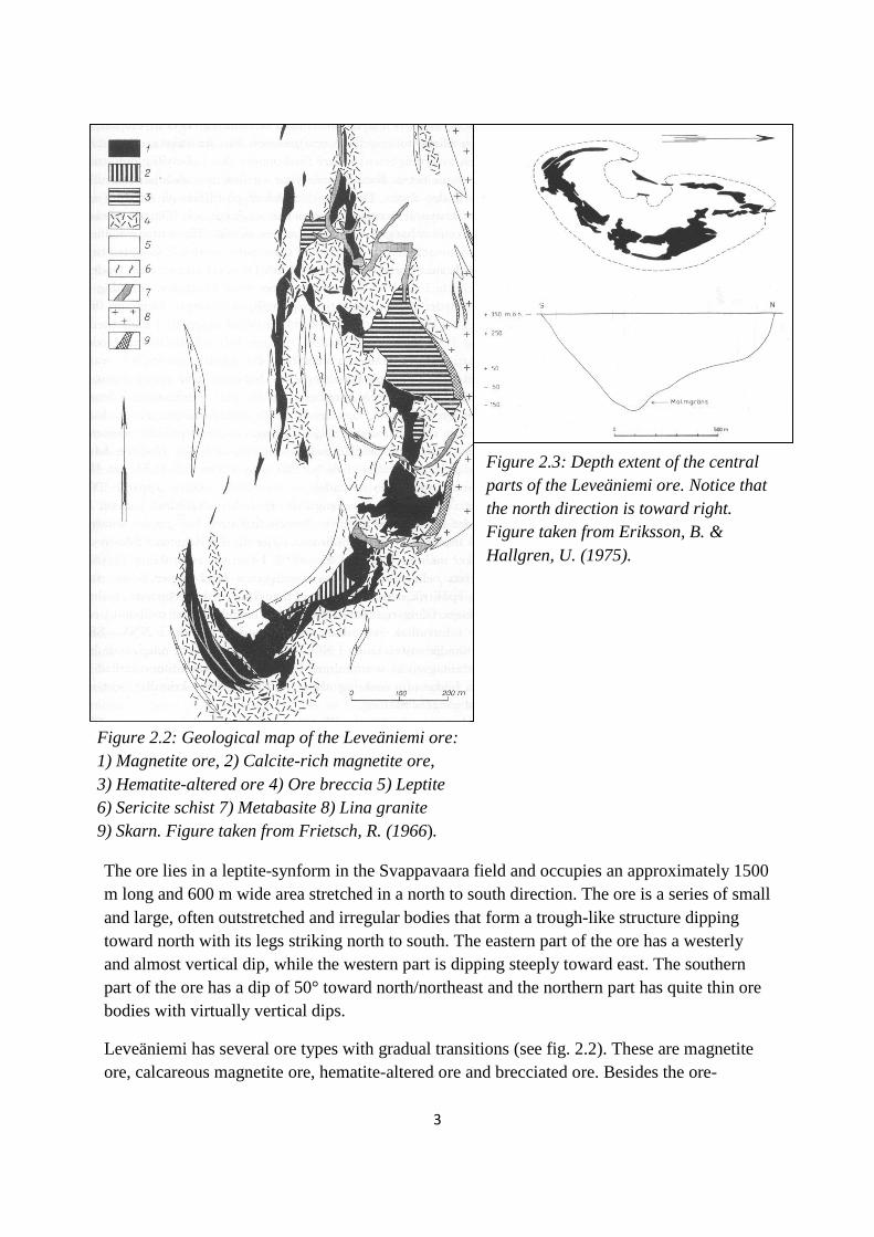
Leveäniemi has several ore types with gradual transitions (see fig. 2.2). These are magnetite

ore, calcareous magnetite ore, hematite-altered ore and brecciated ore. Besides the ore-

Figure 2.2: Geological map of the Leveäniemi ore:

1) Magnetite ore, 2) Calcite-rich magnetite ore,

3) Hematite-altered ore 4) Ore breccia 5) Leptite

6) Sericite schist 7) Metabasite 8) Lina granite

9) Skarn. Figure taken from Frietsch, R. (1966).

Figure 2.3: Depth extent of the central

parts of the Leveäniemi ore. Notice that

the north direction is toward right.

Figure taken from Eriksson, B. &

Hallgren, U. (1975).

4

minerals, the ores mostly consist of apatite, calcite, tremolite-actinolite and biotite (Frietsch,

R., 1966).

The total area of the ore, including the breccia, is 129 500 m2 with a volume in the magnitude

of 300 million metric tons. (Eriksson, B. & Hallgren, U., 1975) The magnetite ore is the major

ore type and constitutes 64 200 m2 of the total area and has an average Fe-content of 63.2%

(Frietsch, R., 1966). The hematite-altered ore has a Fe-content of 64.5% and makes up 25 500

m2 of the total area (Frietsch, R., 1966) It is most common in the central parts of Leveäniemi

where it forms slabs in the magnetite ore that can be as big as 600 m2 (Eriksson, B. &

Hallgren, U., 1975) . 4800 m2 consists of calcite-rich magnetite ore (Fe=64%), which is

concentrated in the southern parts (Frietsch, R., 1966) and characterized by slabs and spots of

white to red-white calcite in the ore. The breccias surround the concentrated ores and can be

as wide as 100 m in some parts. These are composed of a vascular net of magnetite and minor

hematite that increase in size toward the concentrated ores (Eriksson, B. & Hallgren, U.,

1975). The breccias have an average Fe-content of 35.4% (Frietsch, R., 1966).

The depth of the ore (fig 2.3) is greatest in the central parts where it goes down to about 500

m. This is also where the major part of the ore is situated, reaching up to 150 m in width. The

ore in the southern parts only reach shallow depths.

The bedrock that surrounds Leveäniemi is mainly leptites with a syenite-porphyritic

composition (Frietsch, R., 1966). To the west and southwest the ore body is confined by a

sericite-schist that almost entirely consists of muscovite and quartz. The schist has gradual

transitions into the leptite (Eriksson, B. & Hallgren, U., 1975). There also occur intrusive

rocks in the area such as the Lina granite and metabasites (Frietsch, R., 1966).

2.2 Gravimetry

Gravity surveys investigate subsurface geology by measuring variations in Earth’s

gravitational field originating from differences in densities of the bedrock. Rocks that have a

higher density than the surrounding bedrock give rise to positive anomalies and rocks that

have lower densities create negative anomalies.

Differences in rock densities are the least variable property of rocks, typically varying

between 1.60 and 3.20 Mg/m3. The density depends on the rocks porosity and mineral

composition. Higher porosity gives lower density. Magmatic and metamorphic rocks usually

have very low porosity, so their differences are determined mostly by mineral composition

(Kearey, P. et al., 2002).

2.2.1 Theory

The basis of gravimetric surveys is Newton’s law of Gravitation, where the force of attraction

F between two bodies of mass (m1 and m2) separated by the distance r is given by the

equation:

(1) (G=6.67x10-11

m3kg

-1s

-2)

5

If the Earth was a perfect, homogenous and non-rotating sphere with mass M and radius R, the

force of gravity F on a small mass m on its surface would be calculated by equation 2.

Hence, the weight of a mass on the surface of Earth is given by mg (g is the gravitational

acceleration). In this case the gravitation would be the same everywhere on the surface of

Earth. Earth is, however, more shaped like an ellipsoid and has an irregular surface relief,

internal mass distribution and it rotates. This gives rise to variations in the gravitation across

the surface.

The mean value of g at the surface of Earth is about 9.8 m/s2. Variations that rise from sub-

surface differences in densities are in the magnitude of 100 µm/s2 and termed as one gu

(gravity unit). In the c.g.s. system gravitation has the unit milligal (1 mgal = 10-3

gal = 10-3

cm/s2 = 10 gu) (Kearey, P. et al., 2002).

2.2.2 Gravimetric surveys

Since gravity is acceleration, the measurements involve length and time. Measurements of

absolute gravity is complex and time-consuming, therefore gravity surveys often focus on

measuring relative differences of gravity in a given area. The absolute value can be calculated

from the surveys by using a reference point with a known value of absolute gravity, for

instance from the International Gravity Standardization Network (IGSN).

Relative gravitation is measured with an instrument called a gravimeter, whereof the most

common one contains a small, known mass hanging from a spring. The amount of stretching

of the spring depends on the pull of gravitation; therefore readings of the length of the spring

give the relative gravitation (Kearey, P. et al., 2002).

2.2.3 Measurement corrections

Prior to any interpretations of a gravimetric survey the measurement values must undergo a

process called gravity reduction. This process involves a series of corrections for variations in

the gravitational field that do not originate from differences in the sub-surface geology.

Any changes that the instrument may experience during a survey that affect the

measurements, such as heat differences and permanent changes in the length of the spring, are

corrected by regular readings at a base station at recorded times throughout the survey. This is

called drift correction and is assumed to be linear. The difference d at time t is calculated and

then subtracted from the survey values.

The ellipsoid shape of Earth and its rotation give a variation in the force of gravity with

latitude. The gravity is stronger at the poles and weakest at the equator. The effect of this at

different latitudes is calculated with mathematical formulas and is called latitude correction.

6

Tidal variations of gravity emerge from the movements of the moon and the sun that affect

the Earth in the same way as the ocean tide, although not as dramatic. These variations can

either be corrected by frequent base readings or calculated with a computer.

Variations of the elevation between different datum points are corrected by the free-air

correction. To get rid of the effect of different thicknesses of the underlying bedrock resulting

from variations in elevation, a Bouguer-correction is performed. The Bouguer-correction

assumes that the terrain surrounding the datum point is flat, this is most often not the case and

therefore a terrain correction is needed. A terrain correction is always positive and is

calculated from terrain data (Kearey, P. et al., 2002).

2.3 Magnetometry

In magnetic surveys the goal is to investigate sub-surface geology by observing anomalies in

the Earth’s magnetic field. There are only a few rock-types that contain sufficient amounts of

magnetizing minerals to produce anomalies.

The SI unit of magnetic fields is Tesla (T), but this unit is too large for the magnetic

anomalies that arise from magnetizing rocks. Therefore the smaller unit nanoTesla (nT) is

used in magnetic surveys (Kearey, P. et al., 2002).

2.3.1 The geomagnetic field

Earth’s magnetic field, or the geomagnetic field, is believed to be created by the movement of

charged particles in the outer, fluid parts of the Earth’s core (Marshak, S., 2005) and can be

represented by a theoretical dipole at the centre of Earth with an inclination of about 11.5° to

the axis of rotation.

The geomagnetic field at a given point on the Earth is described by a total field vector B that

has a vertical component Z and a horizontal component H pointing toward the magnetic north.

The angle I to Z describes the inclination of the geomagnetic field and the angle D to H

describes the angle of the field relative to the geographic north, called the declination. On the

northern hemisphere the geomagnetic field points downward toward north and on the

southern hemisphere the field points upwards. The field is vertical at the poles and virtually

horizontal at the equator. The geomagnetic field varies in intensity over the Earth’s surface,

from about 25 000 nT at the equator to about 70 000 nT at the poles (Kearey, P. et al., 2002).

The geomagnetic field also changes with time. These are slow secular variations of the angle

D to the geographic North Pole and more rapid, small changes in the magnetic field strength

called diurnal variations. Even the total intensity of the geomagnetic field changes over time.

All these changes can be calculated using complex formulas. The total intensity, inclination

and declination of any place on Earth at a given time can be obtained from the International

Geomagnetic Reference Field (IGRF) (Kearey, P. et al., 2002).

2.3.2 The magnetization of rocks

The magnetizing character of rocks is determined by their susceptibility, which in turn

depends on the content of magnetic minerals in the rocks. There are only two geochemical

7

groups that provide such minerals, the iron-titanium-oxygen group and the iron-sulphur

group. Magnetite (Fe3O4) and hematite (Fe2O3) belongs to the iron oxides. Hematite is,

however, antiferromagnetic and does not give rise to magnetic anomalies unless a parasitic

antiferromagnetism is developed. Magnetite is by far the most common magnetic mineral and

therefore it is possible to classify a rocks magnetic behavior on its overall magnetite content.

In general the proportion of magnetite in igneous rocks tends to decrease with increasing

acidity (Kearey, P. et al., 2002).

2.3.3 Magnetic surveys

If there are rocks with magnetizing characteristics in the survey area, these will give rise to

anomalies in the geomagnetic field. Anomalies are produced either by induced magnetism Ji

or by remanent magnetism Jr. Ji lies in the direction of the inducing field, in this case the

geomagnetic field H, and the strength of Ji is determined by the strength of H and the

susceptibility of the rock. Remanent magnetism is a small, independent magnetic field

preserved from the formation of the rock and can be in virtually any direction. If both an

induced and a remanent field are present the anomaly will be the resultant vector of them. The

ratio Ji:Jr is called the Königsbergs ratio (Q) (Kearey, P. et al., 2002). A high value of Q

means that the remanent magnetization is considerable and should be taken into account

(Mussett, A-E. & Aftab Kahn, M., 2000).

When carrying out a magnetic survey, the difference in the theoretical, undisturbed

geomagnetic field and the observed magnetic field gives the strength and the character of the

anomaly and thus information about the sub-surface geology.

8

3 Data

Both the gravimetric and the magnetic surveys of the Leveäniemi ore are presented in maps

with a scale of 1:5000. The extent of the maps (fig. 3.1) belong to a larger net from 1940-1942

that uses its own coordinate system with westerly and southerly directions and has a local

north direction 39° west of the true north. The maps showing Leveäniemi account for the

square 2000-6000 S and 1500-4000 W in the larger net and also cover the larger ore body of

Gruvberget, hence the name of the maps is “Gruvberget NO” (Espersen, J. & Frietsch, R.,

1964). In this thesis only one half of the maps are used, namely 4000-6000 S and 1500-4000

W which is the part covering the Leveäniemi ore.

Figure 3.1: Map showing the extent of Gruvberget NO (red rectangle) produced by SGU as

well as the geological map of the Leveäniemi ore created by Tibor Parák (map material from

Lantmäteriet).

Gruvberget and Leveäniemi were the first objects to be investigated when SGU started their

work in the area in 1957. The surveys were carried out in the net from 1940-1942 that were

upgraded and densified with additional N-S-lines (Espersen, J. & Frietsch, R., 1964).

9

3.1 Gravimetric data

The gravimetric survey was performed during late summer and autumn in 1957 using SGU’s

gravimeter Worden Pioneer 306. The profiles were laid out north to south every 200 m with a

distance of 40 m between each datum point. Part of the area has been complemented with

closer datum and profile spacing.

The anomaly were calculated in a local system with a base point positioned close to Ny

Kvarnijärvi where the value of g was set to zero and the height was set to +3 m. The absolute

value is zero in the corner of 2000 S/2000 W, which gave a positive latitude correction. This

local system can be re-calculated to absolute values using g = 982.384 gal and a height of

319.480 m at the base point. The true absolute value in the corner 2000 S/2000 W is 982.471

gal. The bouguer-factor used by SGU was 0.1976 mgal/m. The terrain correction for every

datum point has been performed to a radius of 2 km. The regional field has been determined

graphically with the aid of neighbouring areas (Espersen, J. & Frietsch, R., 1964).

According to Espersen, J. & Frietsch, R. (1964), the relative and absolute accuracy of the

measurements are better than 0.03 mgal.

The anomaly has been presented in several two-colored contour maps with thick lines for

every 0.5 mgal and thin lines for every 0.1 mgal (Espersen, J. & Frietsch, R., 1964). The one

depicting the local anomaly is the one used in this thesis.

3.2 Magnetic data

During the same period as the gravimetric survey, a magnetic survey of the vertical intensity

Z was carried out. The survey has E-W profiles with 40 m spacing and datum points every

twentieth meter (10 m where readings exceed 5000 nT). These measurements were later

complemented with intermediate, 20 m E-W profiles with a 10 m datum point distance.

The survey was carried out using a Breen-magnetometer with an addition made by SGU to

expand the measurement interval to 80 000 nT.

Calculations of the observed anomaly refer to a series of control lines to base stations in a

neutral field in Svappavaara village. A normal value for the area was obtained from the

national system through readings at the observatories in Kaupinen and Lovö and was set to

49 600 nT (1958). Corrections for daily variations were performed with readings from the

Kaupinen observatory.

According to control measurements, the anomaly is known with an absolute accuracy of ±50

nT and a local, relative accuracy of ±20 nT.

The magnetic anomaly is presented in a similar way as the gravimetric anomaly, but with

contours drawn according to a logarithmic system with thick lines for ±1000, 2000, 4000,

8000, 16 000, 32 000 and 64 000 nT. Thin lines represent every quarter of the interval

between the thick lines (Espersen, J. & Frietsch, R., 1964).

10

4 Preparatory work

4.1 Digitizing the maps

Prior to importing the values of the anomaly into MVP the maps had to be digitized. This was

done in a similar fashion for both maps.

In addition to containing contours of the anomaly values the maps also contain the actual

value received at the datum points in the survey profiles. These were acquired and transferred

into a computer along with the profile and datum spacing, represented as columns and rows.

For practical reasons some of the more closely spaced, interlaying datum points had to be

neglected. In some places values were missing or could not be read, these points were

accounted for by using NaN in the computer, which interpolated them with surrounding

values in MVP.

The gravimetric digitization resulted in columns for every fortieth meter from 4000 S to 5960

S and rows for every fiftieth meter from 1500 W to 4000 W. The magnetic data had columns

for every fortieth meter from 4000 S to 6000 S and rows for every twentieth meter from 1500

W to 4000 W.

Part of the magnetic map demanded a special method for its digitization. This was necessary

because the central part of the map, where the anomaly was greatest, lacked numbers for a

large area. Therefore a check pattern that corresponded to the other datum points and profiles

was drawn over this area. Values were then extracted where the lines crossed the contours of

the anomaly.

Since the gravimetric map values are represented as gal and MVP uses mgal, the values were

divided by 100. The magnetic values were presented in a unit of 100 gamma and were

converted into nT by multiplying them with a factor of 100.

To be able to import the digital data into MVP the format of the data had to be converted into

Geodesi multi-line files. To do this each row were transformed into a line that contained all

the datum points in that particular row. These lines where then exported to a xyz-file format.

4.2 Setting up Model Vision Pro 9.0

The first step when using MVP is to create a new project. In doing so, the parameters for the

survey values that will be imported later are defined. One such parameter is what unit the

gravimetry is presented in, this was set to the c.g.s. unit mgal for this project. Other

parameters are the inclination, declination and total intensity of the magnetic field in the

region during the time of the survey. These were obtained from a web-based IGRF, provided

by the World Data Center for Geomagnetism in Kyoto, where the coordinates and elevation

for Leveäniemi were put in and the geomagnetic field was obtained. The inclination was set to

76.5° and the declination to 2.8° for the year 1955 (http://wdc.kugi.kyoto-u.ac.jp/index.html).

The total intensity was set to 49 600 nT, which is the total intensity that was used by SGU in

their calculations (Espersen, J. & Frietsch, R., 1964).

11

When defining the project there is also the possibility to choose what coordinate system the

measurement points are presented in. It is possible to choose from a number of different

international systems, national systems and to create a local XY-system. The later was chosen

for this project, since the system used by SGU was a local XY-system.

When a project has been defined all the work and created displays will be saved in a session

file, while the raw data and parameters, as well as the session file will be saved in the project

directory.

4.3 Data import and preparations for modeling

Data are imported into MVP using its import function. While this function supports a wide

range of data-files, the ones that resulted from the digitization process were line-data files in

the Geodesi multi-line format. Because of the nature of line-data, they are only possible to be

displayed in MVP as lines with a related graph that represent the values.

To create contour-maps resembling those in the original maps and to be able to create cross-

sections for modeling, the line-data for both the gravimetric and magnetic data had to be

converted into grids. This was done by using the grid channel data where grids can be created

from line data. The resulting grid, as well as the original line-data, was up-side-down when

displayed. In the grid utility this could be corrected with the flip grid function. The flipped

grids were saved as new grid files.

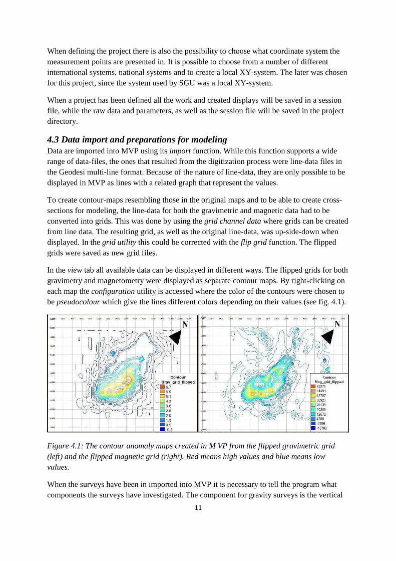
In the view tab all available data can be displayed in different ways. The flipped grids for both

gravimetry and magnetometry were displayed as separate contour maps. By right-clicking on

each map the configuration utility is accessed where the color of the contours were chosen to

be pseudocolour which give the lines different colors depending on their values (see fig. 4.1).

Figure 4.1: The contour anomaly maps created in M VP from the flipped gravimetric grid

(left) and the flipped magnetic grid (right). Red means high values and blue means low

values.

When the surveys have been in imported into MVP it is necessary to tell the program what

components the surveys have investigated. The component for gravity surveys is the vertical

12

component by default, but for the magnetic survey it was necessary to change this from the

total field to the vertical component. This was done for the line and grid data, as well as for

what component the program should model the theoretical anomaly of created bodies in.

4.4 The coordinate issue

In addition to the features of the ore described in section 2.2, a digitized geological map of the

Leveäniemi ore and its immediate surroundings was available for this thesis. The geological

map was produced by Tibor Parák in his investigations of the ore body made for SGU in 1964

and was obtained from the Malå archives.

As mentioned before, the geophysical surveys used a local coordinate system. This is also true

for the geological map of the Leveäniemi ore made by Tibor Parák, but its local coordinate

system is different from the one in the geophysical maps.

To be able to overlay the geological map on the contour maps in MVP without any

distortions, the local coordinate systems had to be transformed into a common coordinate

system. This was done in several steps.

An Excel-file provided by Anders Hallberg at SGU contained trigonometric formulas for

transforming local coordinates into SWEREF 99 TM coordinates. The formulas required the

angle of the local system to the true north, its zero point and a few control points to check the

accuracy.

Only two control points were found in both the local maps and in maps that were downloaded

from the digital map library at Lantmäteriet (https://butiken.metria.se/digibib/index.php).

These were defined in SWEREF 99 TM coordinates using arcGIS. The angle to the true north

was set to 321°, which corresponds to 39° to the west. An approximate zero point was found

using the Direction-Distance Tool in arcGIS and described in SWEREF-coordinates. The zero

point was then calibrated until the control point coordinates found in arcGIS corresponded to

the coordinates resulting from the formulas. The SWEREF-coordinate system, as well as the

formula, uses northerly and easterly directions. The local system, on the other hand, uses

southerly and westerly directions and was therefore put into the formula as negative values.

The geological map made by Tibor Parák is used in the SGU-report Series C No. 604,

although slightly modified (fig. 2.2). The map was cut down in size to correspond to the one

used in Series C No. 604 and geo-referenced in arcGIS using its square extent that are defined

in a supplementary map. The position of the geological map is displayed in fig. 3.1. The

SWEREF-coordinates for the geological map extent was then transformed into the local

coordinates of the SGU-surveys by using the Excel-file in reverse. This made it possible to

import it into MVP and roughly placing it over the contour maps, avoiding any distortions.

4.5 Rock densities

Prior to the gravimetric modeling, the densities of the different ores had to be estimated. The

average Fe-content of the different ores is known and was assumed to originate mostly from

the ore minerals themselves. Magnetite has a density of 5.18 Mg/m3 and pure hematite has a

13

density of 5.25 Mg/m3 (Nesse, W. D., 2000), but since the hematite ore also contains

magnetite they should be similar.

The remaining percentage of the ores was dedicated to an average of the densities of the other

minerals constituting the ores. These are apatite (3.1-3.35 Mg/m3), calcite (2.71 Mg/m

3),

tremolite-actinolite (2.9-3.48 Mg/m3) and biotite (2.7-3.3 Mg/m

3) (Nesse, W. D., 2000).

These gave an average density of 3 Mg/m3. The average density of the remaining minerals in

the calcite-rich ore was set to a slightly lower value of 2.8 Mg/m3 because of the larger

amount of calcite.

The material of the breccia, other than the ore, has a similar composition as the surrounding

country rock (Frietsch, R., 1966). Measurements of the densities of rocks in the proximity of

Leveäniemi were obtained from the SGU database and showed densities of approximately 2.7

Mg/m3.

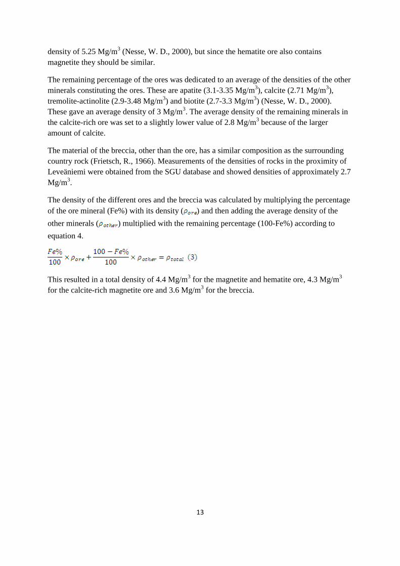
The density of the different ores and the breccia was calculated by multiplying the percentage

of the ore mineral (Fe%) with its density ( ) and then adding the average density of the

other minerals ( ) multiplied with the remaining percentage (100-Fe%) according to

equation 4.

This resulted in a total density of 4.4 Mg/m3 for the magnetite and hematite ore, 4.3 Mg/m

3

for the calcite-rich magnetite ore and 3.6 Mg/m3 for the breccia.

14

5 Modeling

5.1 3D-model generator

MVP has a function called 3D-model generator which makes it possible to draw the outline of

3D-bodies in map view with a certain depth extent. This method seemed suitable for this

project considering the available geological information. Several bodies were created

representing the different ore types in the geological map (fig. 5.1), but it turned out that the

shape and depth extent of the models created with this tool was not possible to alter in cross-

section, which was necessary because of the complicated structure of the Leveäniemi ore.

MVP has the ability to import complex 3D-models in this mode, but for this thesis the ore

body had to be created in MVP itself.

Figure 5.1: Bodies created in MVP using the 3D-model generator tool.

5.2 Cross-sections

The second approach of modeling was initiated by the creation of a series of cross-sections

traversing the anomaly maps in an east-west direction, perpendicular to the main strike of the

ore. The cross-sections were drawn out in the contour maps using the create traverse button,

which creates new lines with anomaly curves that are interpolated from the grids. When a line

has been drawn the name of the new cross-section can be typed in, as well as what grids it

should interpolate the anomaly curves from. Fifteen profiles were drawn in map view as seen

in fig. 5.2.

15

Figure 5.2: Gravimetric anomaly (red contours) and the modified geological map of the

Leveäniemi ore (made by Tibor Parák) with the created cross-sections (blue lines). Cross-

section one is the bottommost line and cross-section fifteen is the uppermost line. The circles

a and b mark erroneous values found in the grid.

When the cross-sections have been saved, they can be viewed with the view X-section

function. A window appears where the chosen line and interpolated anomaly curves are

displayed. Two-dimensional bodies can then be created in the cross-sections and extended in

width to create a three-dimensional body.

The bodies that are created in MVP produce a new anomaly grid from which a theoretical

response curve in each cross-section is obtained. The goal is to create bodies that have a

response curve corresponding to the observed anomaly in each cross-section.

5.3 Gravimetric modeling

The first anomaly to be modelled was the gravimetric anomaly. In MVP it is possible to set a

background value for the survey and in accordance with the data from SGU this was set to 2.7

Mg/m3.

Given the surface extent of the ore, the known dips, depth extent and general features of the

ore body, several two-dimensional bodies with the calculated densities were created in each

16

cross-section starting with the southernmost cross-section 1. MVP has a series of basic

geometric shapes to choose from, as well as the option of creating polygons of any shape.

Since the ore in Leveäniemi has a quite complex structure the polygon was the most adequate

option. The polygons were then extended in width until they connected between the cross-

sections and were set to have an azimuth of 39°, thereby striking in a north-south direction.

The polygons were manually altered through trial and error in each cross-section until their

theoretical anomaly curve resembled the observed gravimetric anomaly, a method also called

forward modeling (Reference Manual, 2009).

Erroneous values were discovered in two places in the gravimetric anomaly map in MVP (see

fig. 5.2), namely the large peak in cross-section 15 (b) and the peak far to the left in cross-

section 12 (a). In cross-section 15 one datum point had been put in as 5.35 mgal instead of

0.53 mgal and in cross-section 12 the value should be 1.62 mgal instead of 6.62 mgal. It was

difficult to correct these false values in the existing grid since these contain interpolated

values from the line-data. But even when a new, corrected grid had been created it seemed as

if the anomaly curves in the created cross-sections were locked to the old grid that the cross-

sections were drawn in.

5.4 Magnetic modeling

When the shape, depth extent and general appearance of the ore had been determined in the

gravimetric modeling, the magnetic anomaly could be modeled using the MVP inversion tool.

The magnetic anomaly map was selected for modeling and all the cross-sections along with

their polygons were chosen to be active lines.

The inversion tool has a number of parameters that can be set free in the inversion process,

but since the position, shape, depth extent and size of the bodies already had been defined, the

only free parameter used in the inversion was the properties parameter. This restricted the

program to only alter the susceptibility of the bodies. Since the country rock that surrounds

the ore mostly has a felsic composition (Frietsch, R., 1966) and therefore low susceptibilities

(Kearey, P. et al., 2002), the default background susceptibility of zero in MVP was retained.

The inversion process was carried out a number of times with increasing tolerance until the

theoretical response curve (red line) resembled the observed anomaly (fig. 5.3).

17

Figure 5.3: The magnetic anomaly curve in cross-section 1 resulting from the inversion

process.

The inversion did not yield any good results. The response curve did not closely resemble the

observed anomaly and some of the susceptibilities came out as negative values, which is not

plausible. According to the MVP help manual, an inversion resulting in negative values

indicates that a remanent magnetization is present.

The inversion tool is capable of estimating the remanent magnetization if the susceptibility of

a body is known, but since neither was known for this modeling there were essentially too

many unknowns to be able to make a reasonable modeling of the anomaly. Therefore the

magnetic modeling in this thesis should merely be seen as a test of the inversion tool.

18

6 Results

All the cross-sections with the observed and the modelled anomaly for the gravimetry and

magnetics, as well as the created polygons, are presented in Appendix 1. The uppermost graph

is the gravimetric anomaly where the black line represents the observed gravimetric anomaly

and the blue line represents the modelled gravimetric anomaly. The bottom graph is the

observed magnetic anomaly (black line) and the modelled magnetic anomaly (red line)

created in the inversion process. The polygons that produce the theoretical anomaly are

displayed below the graphs and in fig. 6.1 the polygons from each cross-section are displayed

as they appear in the map view. The properties of all the created polygons are presented in

Appendix 2.

Figure 6.1: The created polygons displayed in map view.

When the polygons from the different profiles have been stretched out in width they create a

three-dimensional body as seen in the perspective view in fig. 6.2.

19

Figure 6.2: The final 3D-model resulting from the gravimetric modeling.

The body displayed in fig. 6.2 is based on the polygons that were created in the gravimetric

modeling. As mentioned before, the polygons produce a grid with a theoretical anomaly in

MVP. Grids can also be viewed in three dimensions with the perspective view. In fig. 6.3 the

anomaly grid from the gravimetric modeling is compared with the corrected, observed

anomaly grid from the survey.

20

Figure 6.3: Comparison between the observed gravimetric anomaly grid (top) and the created

gravimetric anomaly grid (bottom) resulting from the created polygons displayed in

perspective view. Dark-blue areas are not covered by the modeling.

21

7 Discussion

Geological information is essential in giving guidelines to what a body that creates an

observed anomaly may look like. When the geological information is limited the modeling

basically becomes an exercise in successive approximation. On the other hand, the lack of

available geological information often is one of the reasons to making a geophysical

interpretation.

The available geological information for this thesis was quite comprehensive, but the placing

of the geological map may not be entirely correct because of the different coordinate systems.

A major problem in modeling, such as the one performed in this thesis, is that it assumes that

the world is homogeneous. The background density was set to 2.7 Mg/m3 with the assumption

that everything, other than the ore, has the same density, which of course is not true. Even the

different ore types are assumed to be homogenous with the same density everywhere, while in

reality the ore grade and thereby the density is likely to vary throughout the ore bodies.

Some of the cross-sections have a good correlation with the observed gravimetric anomaly,

while others do not match it as good. Forward modeling is a time-consuming task and

eventually the model had to be considered satisfactory for the second part of the modeling,

namely the inverse modeling of the magnetic anomaly. But as seen in the comparison between

the 3D-grid of the observed anomaly and the modeled anomaly (fig. 6.3), they have a fairly

good match.

The inversion tool in MVP is a powerful tool, but it should be used with caution. In the early

stages of the gravimetric modeling the inversion tool was tested on the created polygons in the

pursuit of finely adjusting their shape and size. But since the program takes no regard to the

known geological features the resulting bodies could look very strange and erroneous. The

inversion tool was used in the magnetic modeling, but the number of unknown parameters is

too numerous for a plausible result.

8 Conclusions

Model Vision Pro 9.0 truly is an interactive modeling program. With the creation of polygons

in cross-section view it is possible to create bodies freely and modifying them as you like. The

capability to modify the bodies in the third-dimension with this method is rather limited, but

this is not very surprising since such modifications are very complex and the risk of crossing

edges becomes imminent.

The inversion tool has many features and can be quite daunting to understand. The inversion

tool has been tested in this thesis, but its usage was rather restricted by lack of information

and it is evident that the tool has far more capabilities. This insight is true for Model Vision

Pro 9.0 as a whole. Even though many of its functions have been tested in this thesis it seems

like this work only has scratched the surface of the programs full capacity.

22

The model that was created in this thesis seems to confirm previous conclusions about the

features and depth extent of the Leveäniemi ore. It is evident that it has been subjected to at

least one folding event and that it forms a trough-like structure dipping toward north with the

main ore-volume concentrated to the central parts.

9 Acknowledgements

First of all I would like to thank my supervisor Erik Sturkell for assigning me to this project

and for his guidance throughout the work. I would also like to thank Danial Farvardini for

getting me started with the digitization process and helping me with Model Vision Pro 9.0.

Last, but not least, I want to thank Anders Hallberg at SGU for helping me solve the

coordinate issue and providing me with the transformation Excel-file.

23

10 References

Eriksson, B. & Hallgren, U., 1975: Description of the Geological Maps Vittangi NV, NO, SV,

SO. Series Af: No. 13-16, SGU. 146-147

Espersen, J. & Frietsch, R., 1964: Gruvbergets järnmalmsförekomst. SGU. 99-102.

Frietsch, R., 1966: Berggrund och malmer I Svappavaarafältet, Norra Sverige. Series C. No.

604. SGU. 184-187.

Kearey, P., Brooks, M. & Hill, I., 2002: An Introduction to Geophysical Exploration, Third

Edition. Blackwell Science Ltd. And references used in that book. 125-139, 155-166.

Marshak, S., 2005: Earth: Portrait of a Planet, Second Edition. W. W. Norton & Company,

Inc. 55.

Mussett, A-E. & Aftab Kahn, M., 2000: Looking into the Earth: An Introduction to

Geological Geophysics. Cambridge University Press. 172-173.

Nesse, W. D., 2000: Introduction to Mineralogy. Oxford University Press, Inc. 246, 283, 329,

346, 360, 364.

Parák, T., 1964: Geological map of Leveäniemi obtained from the Malå archives.

Reference Manual, 2009: Encom Model Vision Pro 9.0.

10.1 WebPages

Lantmäteriet: https://butiken.metria.se/digibib/index.php (2010-05-06)

http://www.lkab.com/?openform&id=17ACE (2010-06-01)

http://wdc.kugi.kyoto-u.ac.jp/igrf/index.html (2010-03-05)

24

Appendix 1, cross-sections

25

26

27

28

Appendix 2, polygon table