University of Groningen

A method to reduce the spin-up time of ocean modelsBernsen, Erik; Dijkstra, Henk A.; Wubs, Fred W.

Published in:Ocean modelling

DOI:10.1016/j.ocemod.2007.10.008

IMPORTANT NOTE: You are advised to consult the publisher's version (publisher's PDF) if you wish to cite fromit. Please check the document version below.

Document VersionPublisher's PDF, also known as Version of record

Publication date:2008

Link to publication in University of Groningen/UMCG research database

Citation for published version (APA):Bernsen, E., Dijkstra, H. A., & Wubs, F. W. (2008). A method to reduce the spin-up time of ocean models.Ocean modelling, 20(4), 380-392. https://doi.org/10.1016/j.ocemod.2007.10.008

CopyrightOther than for strictly personal use, it is not permitted to download or to forward/distribute the text or part of it without the consent of theauthor(s) and/or copyright holder(s), unless the work is under an open content license (like Creative Commons).

Take-down policyIf you believe that this document breaches copyright please contact us providing details, and we will remove access to the work immediatelyand investigate your claim.

Downloaded from the University of Groningen/UMCG research database (Pure): http://www.rug.nl/research/portal. For technical reasons thenumber of authors shown on this cover page is limited to 10 maximum.

Download date: 27-05-2020

Available online at www.sciencedirect.com

Ocean Modelling 20 (2008) 380–392

www.elsevier.com/locate/ocemod

Short communication

A method to reduce the spin-up time of ocean models

Erik Bernsen a,*, Henk A. Dijkstra a, Fred W. Wubs b

a Institute for Marine and Atmospheric Research Utrecht, Department of Physics and Astronomy, Utrecht University,

3584CC Utrecht, The Netherlandsb Department of Mathematics and Computer Science, University of Groningen, Groningen, The Netherlands

Received 12 July 2007; received in revised form 23 October 2007; accepted 23 October 2007Available online 22 November 2007

Abstract

The spin-up timescale in large-scale ocean models, i.e., the time it takes to reach an equilibrium state, is determined bythe slow processes in the deep ocean and is usually in the order of a few thousand years. As these equilibrium states aretaken as initial states for many calculations, much computer time is spent in the spin-up phase of ocean model computa-tions. In this note, we propose a new approach which can lead to a very large reduction in spin-up time for quite a broadclass of existing ocean models. Our approach is based on so-called Jacobian–Free Newton–Krylov methods which com-bine Newton’s method for solving non-linear systems with Krylov subspace methods for solving large systems of linearequations. As there is no need to construct the Jacobian matrices explicitly the method can in principle be applied to exist-ing explicit time-stepping codes. To illustrate the method we apply it to a 3D planetary geostrophic ocean model with prog-nostic equations only for temperature and salinity. We compare the new method to the ‘ordinary’ spin-up run for severalmodel resolutions and find a considerable reduction of spin-up time.� 2007 Elsevier Ltd. All rights reserved.

1. Introduction

Once a large-scale ocean model code has been designed, the first long computations usually performed areaimed to determine an equilibrium state of the model under given forcing. The time-scale to reach equilibriumdepends on the vertical diffusion of salinity and temperature and is given by D2=jv where D is a characteristicdepth of the ocean basin and jv is the vertical diffusivity. For typical values of jv ¼ 10�5 m2 s�1 andD ¼ 103 m, this so-called spin-up time-scale is approximately 3000 years. When the ocean model uses an expli-cit time-stepping method, then numerical stability conditions (such as the CFL condition) pose limitations onthe time step. In many cases, the computation of equilibrium solutions therefore consumes a lot of CPU time.

A classical method for reducing spin-up time is the method of distorted physics (Bryan, 1984). In thismethod, the model equations are adjusted such that the equilibrium solutions are unchanged but the slowprocesses in the deep ocean are artificially accelerated. This method has been implemented successfully in

1463-5003/$ - see front matter � 2007 Elsevier Ltd. All rights reserved.

doi:10.1016/j.ocemod.2007.10.008

* Corresponding author. Tel.: +31 30 2532978; fax: +31 30 2543163.E-mail address: E.Bernsen@phys.uu.nl (E. Bernsen).

E. Bernsen et al. / Ocean Modelling 20 (2008) 380–392 381

many existing ocean models but as there remain limitations on the time step in the deep ocean it may still takemuch CPU time.

Another method of reducing the spin-up time is based on exponential extrapolation (Klinger, 2000). A longperiod of the spin-up consists of an almost exponential decay of the temperature and salinity fields towardstheir equilibrium values. Repeatedly extrapolating salinity and temperature based on the assumption of expo-nential decay resulted in a reduction of spin-up time of approximately a factor two to three.

Recently, Khatiwala et al. (2005) presented a method for determining equilibrium states of passive tracers.In this method a transport matrix, the matrix representation of the linear advection–diffusion equation thatgovern the evolution of passive tracers, is computed by performing a number of time steps of the modelfor several tracer distributions. Once this transport matrix is determined, the equilibrium fields for passivetracers are obtained by solving a matrix equation. It was shown in Khatiwala et al. (2005) that a similarmethod can also be applied successfully to active tracers such as temperature and salinity.

With fully implicit ocean models (e.g. Dijkstra et al., 2001; Weijer et al., 2003; De Niet et al., 2007), one cantake relatively large time steps. For example, in Dijkstra et al. (2001) it is shown that in the approach toequilibrium, time steps of 10–100 year can be taken such that the equilibrium state is quickly reached. Thefully-implicit methods, however, have the drawback that an explicit Jacobian matrix of the model has to beavailable. The latter is not easily computed for existing explicit ocean models. In addition, sophisticated pre-conditioners are needed to solve the giant systems of linear equations which result from the Newton–Raphsonmethod during an implicit time step.

In this paper, we present a method for reducing the spin-up time in explicit ocean models by combiningelements from the fully-implicit approach with Jacobian–Free Newton–Krylov (JFNK) methods (Reisneret al., 2000, 2003; Knoll and Keyes, 2004; Knoll et al., 2005). Essentially we apply Newton’s method forobtaining an equilibrium solution to an explicit model but we solve this problem without having to constructthe Jacobian matrix explicitly. Instead only matrix–vector products for the Jacobian are needed and these canbe obtained from the explicit model.

The general methodology is presented in Section 2. Next we apply it to a relatively simple 3D planetarygeostrophic model (Samelson and Vallis, 1997a,b), as described in Section 3.1. Details on the specific imple-mentation of the JFNK method for this model are given in Section 3.2. In Section 4, we compare the spin-upresults of the JFNK method with those of the explicit time-stepping method and in Section 5, we drawconclusions and discuss further applications of the JFNK method.

2. The JFNK method

After discretizing the governing equations in space, each ocean model can in general be cast into the fol-lowing form:

d~xdt¼ ~F ð~x; lÞ; ð1Þ

where~x is the state vector containing all prognostic variables on all the grid points and ~F ð~x; lÞ is usually re-ferred to as the residual. The parameter l is a control parameter for the forcing of the model (wind stress,buoyancy flux) with l ¼ 0 corresponding to no forcing and l ¼ 1 corresponding to the desired forcing.

Traditionally the equilibrium solution is reached by integrating (1) forward in time until we are closeenough to a steady state; so in fact we are solving the nonlinear equation

~F ð~x; lÞ ¼ 0: ð2Þ

As an alternative one can use Newton’s method for solving the system of Eq. (2). Here, we start from an initialguess~x0 and apply the iteration

~xkþ1 ¼~xk þ d~xkþ1: ð3Þ

In this equation, d~xkþ1 is satisfying

D~xk~F d~xkþ1 ¼ �~F ð~xk;lÞ; ð4Þ

382 E. Bernsen et al. / Ocean Modelling 20 (2008) 380–392

where D~xk~F is the Jacobian matrix of ~F at~xk. If we want to apply this method to an existing time-stepping code

the residual ~F is available but the problem is that the Jacobian matrix D~xk~F is in general not easily extracted.

In a Jacobian–Free Newton–Krylov (JFNK) method, the system (4) is solved using a Krylov method, forexample, the GMRES (Saad, 1996, 2003) method. This is an iterative method in which at the lth iteration thesolution of the system (4), more conveniently written as Akd~xkþ1 ¼~bk with Ak ¼ D~xk

~F and ~bk ¼ �F ð~xk; lÞ, isapproximated with a vector d~xkþ1;l from the subspace d~xk;0 þ Kl with the Krylov subspace given by

Kl ¼ ~rkþ1;Ak~rkþ1;A2k~rkþ1; . . . ; . . . ;Al�1

k ~rkþ1

� �ð5Þ

and~rkþ1 ¼ Akd~xkþ1;0 �~bk. The choice of d~xkþ1;l is such that the 2-norm of the residual of the matrix equationjjAkd~xkþ1;l �~bkjj2 is minimized. As the Krylov subspace is extended with one dimension at each iteration, thenorm of the residual of the matrix equation is decreasing with iteration number and in that sense d~xk;lþ1 will bea better approximate solution than d~xk;l. Since the construction of these Krylov subspaces only require matrix–vector products we don’t need the matrix Ak itself, but rather the matrix applied to a vector~v. With Ak ¼ D~xk

~F ,the matrix vector product can be approximated using the finite difference approximation

D~xk~F~v ¼

~F ð~xk þ �~vÞ �~F ð~xkÞ�

þ Oð�Þ ð6Þ

with � ¼ �0ð1þ jj~xkjj1=NÞ=jj~xkjj � 1, N the dimension of the vector ~xk, jj~vjj1 ¼Pjvij and for example,

�0 ¼ 10�6.For a fast convergence rate of the GMRES method a preconditioner may be needed. When using a precon-

ditioner P�1 on a linear system A~x ¼~b, we solve the equivalent system

P�1A~x ¼ P�1~b: ð7Þ

Requirements of a good preconditioner are that P�1 � A�1 such that P�1A is well conditioned and that P�1~v isrelatively easy to compute. The construction of a preconditioner is usually model dependent and hence wedescribe it in the following section after the presentation of our demonstration model.

3. Test case

In this section we describe the implementation of the JFNK method to the planetary geostrophic oceanmodel as developed in Samelson and Vallis (1995, 1997a,b). Details of the model are presented in Section3.1 below; these are not only for convenience for the reader but they are also important for the descriptionof the preconditioner in Section 3.2.

3.1. Planetary geostrophic model

The model we discuss here is a good prototype model since temperature and salinity are the only prognosticvariables and it is the slow transport in the deep ocean of these quantities that causes the extremely long spin-up times. The geometry of the model consists of a rectangular basin of dimension Lx � Ly ¼ 6000 km�6000 km. The bottom is at a constant depth D ¼ 5000 m. In the interior, �D < z < 0, the evolution oftemperature and salinity is governed by the advection–diffusion equations

oTotþ~uh � rhT þ w

oToz¼ o

ozjv

oToz

� �þ jhr2

hT � kr4hT ; ð8aÞ

oSotþ~uh � rhS þ w

oSoz¼ o

ozjv

oSoz

� �þ jhr2

hS � kr4hS: ð8bÞ

E. Bernsen et al. / Ocean Modelling 20 (2008) 380–392 383

In these equations, T is the temperature, S the salinity, jh ¼ 103 m2 s�1 the horizontal Laplacian diffusivity,k � 0:5� 1014 m4 s�1 the horizontal biharmonic diffusivity, jv the vertical diffusivity,~uh ¼ ½u; v�T the horizon-tal velocity field, w the vertical velocity and rh ¼ ½o=ox; o=oy�T the horizontal gradient operator.

For the horizontal momentum equations the geostrophic balance with a linear friction term is used

f~u?h ¼ �rhpq0

� �b~uh ð9Þ

with f ¼ f0 þ by the Coriolis parameter on a b-plane, f0 ¼ 8:4� 10�5 s�1, b ¼ 1:85� 10�11 m�1 s�1, p thepressure, �b ¼ 0:42� 10�5 s�1 the linear friction coefficient, q0 ¼ 103 kg m�3 a reference density and ~u?h ¼½�v; u�T. Finally, the system of equations is completed by the hydrostatic balance, the continuity equationand a linear equation of state

opoz¼ �gq; ð10aÞ

rh �~uh þowoz¼ 0; ð10bÞ

q ¼ q0 1þ aSðS � S0Þ � aTðT � T 0Þð Þ: ð10cÞ

Here, g ¼ 9:8 m s�2 is the acceleration of gravity, aT ¼ 1:0� 10�3 K�1 the coefficient of thermal expansion,aS ¼ 7:6� 10�4 psu�1 the coefficient of saline contraction, and T 0 and S0 are a reference temperature andsalinity, respectively.

Lateral boundary conditions are given by no heat and salinity flux

rhðjhT � kr2hT Þ � n ¼ 0; ð11aÞ

rhðjhS � kr2hSÞ � n ¼ 0; ð11bÞ

with n ¼ ½nx; ny �T the outward normal vector. A second pair of lateral boundary conditions is given by

�brT � nþ frT � s ¼ 0; ð12aÞ�brS � nþ frS � s ¼ 0; ð12bÞ

with s ¼ ½�ny ; nx�T tangential to the boundary. Note that the biharmonic diffusion in (8) allows for two lateralboundary conditions for temperature and salinity and that the boundary conditions (12) ensure consistencywith the lateral boundary conditions for velocity~uh � n ¼ 0. At the bottom we have the no-normal flow bound-ary condition (w = 0) and no heat and salinity flux.

The model is forced by a wind stress and a buoyancy flux applied to an upper explicit Ekman layer with athickness dE ¼ 25 m. The wind stress is given by

~s ¼ l 0; s0

ff0

sinð2py=LyÞ� �T

; ð13Þ

with the maximum amplitude given by s0 ¼ 10�1 Pa. The resulting horizontal and vertical velocity field in theEkman layer are then given by~uE;h ¼~s?=f dE and wE ¼ �dErh �~uE;h respectively. The vertical velocity in theEkman layer acts as a boundary condition for the vertical velocity field in the interior. The horizontal velocityfield is used in the prognostic equations for temperature and salinity in the Ekman layer which become

oT E

otþrh � ð~uE;hT EÞ ¼

F T � F T;i

dE

; ð14aÞ

oSE

otþrh � ð~uE;hSEÞ ¼

F S � F S;i

dE

: ð14bÞ

The heat and salt fluxes between the base of the Ekman layer and the interior are given by

F T;i ¼ wET � 2jv

oToz

� �z¼0

; ð15aÞ

384 E. Bernsen et al. / Ocean Modelling 20 (2008) 380–392

F S;i ¼ wES � 2jv

oSoz

� �z¼0

; ð15bÞ

while the restoring conditions are given by

F T ¼ �s�1T ðT E � T sÞ; ð16aÞ

F S ¼ �s�1S ðSE � SsÞ; ð16bÞ

where sT ¼ sS � 20 days are the relaxation times for temperature and salinity. The surface temperature andsalinity are chosen as

T s ¼ T 0 þlDT cosðpy=LyÞ

2; ð17aÞ

Ss ¼ S0 þlDS cosðpy=LyÞ

2; ð17bÞ

where the temperature and salinity difference between the northern and southern boundary given byDT ¼ 25 K and DS ¼ 1 psu.

Convective adjustment was implemented in Samelson and Vallis (1995) by eliminating all static instabilitiesinstantaneously at the end of each time step. In order to apply the JFNK method it is necessary that the resid-ual ~F can be extracted from the time-stepping code and that this residual is differentiable. Using the convectiveadjustment scheme as in Samelson and Vallis (1995) this is impossible and therefore we implemented it differ-ently using a variable vertical diffusivity given by

jv ¼jv;0 if N 2

b P 0;

jv;0 �aj2

v;CN2

b

1�ajv;CN2b

if N 2b < 0;

8<: ð18Þ

with jv;0 ¼ 10�4 m2 s�1, jv;C ¼ 0:99� 10�2 m2 s�1, the buoyancy frequency Nb given by

N 2b ¼ �

gq0

oqoz;

and the scaling parameter a ¼ 3:89� 103 s3 m�2. Because of this alternative convective adjustment formula-tion, the time-stepping code had to be slightly modified. We used the second order Runge–Kutta schemefor both advection and diffusion where the vertical diffusion is treated implicitly to avoid a severe restrictionon the time step due to convective adjustment.

To write the planetary geostrophic model in the form of (8) we introduce the dimensional state vector~x0 ¼ ð~x0T;~x0SÞ with~x0T and~x0S vectors containing the temperature and salinity at all gridpoints, respectively. Notethat the velocity field is not contained in the state vector since it is diagnostic rather than prognostic. Thedimensional residual is written as ~F 0 ¼ ð~F 0T; ~F 0SÞ, where ~F 0T and ~F 0S are obtained from the discretized versionof (8a) and (8b), respectively. The JFNK and time-stepping method both use a dimensionless state vectorand residual rather than the dimensional ones. Using scales of temperature and salinity variations given bybT � 8:6� 10�3 K and bS � 1:1� 10�2 psu, respectively, and a time scale of t � 1:6 � 102 years, we obtain thedimensionless state vector ~x ¼ ð~xT;~xSÞ ¼ ð~x0T=bT ;~x0S=bSÞ and the dimensionless residual ~F ¼ ð~F T; ~F SÞ ¼ððt=bT Þ~F 0T; ðt=bSÞ~F 0SÞ.3.2. Preconditioner

It turns out that we need to use a preconditioner to speed-up the convergence rate of the GMRES methodin the JFNK method. In our approach for the preconditioner, we first construct the Jacobian or an approx-imation thereof and store this in sparse format. From this we construct a preconditioner using MRILU (Bottaand Wubs, 1999). Since the construction of the matrix in sparse format and the corresponding preconditioneris a relative expensive operation compared to applying GMRES iterations we choose to construct the precon-ditioner once, for the first initial guess for Newton’s method and then reuse this preconditioner for subsequentNewton iterations.

E. Bernsen et al. / Ocean Modelling 20 (2008) 380–392 385

For the construction of the Jacobian matrix (or approximation) we use a technique developed by Colemanet al. (1984). This technique is designed to evaluate a sparse matrix A using as few as possible matrix vectorproducts A~v. Assume that the sparsity pattern of the matrix A is known. In (Coleman et al., 1984) a partitionC1;C2; . . . ;Cp of the columns of A is found such that no pair of columns in the same Cq shares a non-zeroelement on the same row. Then by performing the matrix vector product A~v with vi ¼ 0 if i 62 Cq and vi ¼ 1if i 2 Cq the columns Cq of the matrix A can be obtained. Since for each row of A which contains a non-zeroelement in column k 2 Cq and because no other column in Cq contains a non-zero element in this row, we havethat

Aik ¼Xj2Cq

Aijvj ¼X

j

Aijvj ¼ ðA~vÞj: ð19Þ

For the planetary geostrophic model, the residual for the temperature equation in gridpoint ði; j; kÞ depends onT i;j;k, Si;j;k, T i�1;j;k, T i;j�1;k, T i�2;j;k, T i;j�2;k, T i;j;k�1 and Si;j;k�1 for the horizontal and vertical diffusion and for theadvection terms it depends additionally on ui�1=2;j;k, vi;j�1=2;k and wi;j;k�1=2. Since the velocity field is diagnostic,the velocities themselves depend on temperature and salinity. For instance, it turns out that the velocityui�1=2;j;k depends on T iþ1=2ð1�1Þ;j;: and Siþ1=2ð1�1Þ;j;:, thus the velocities depend on whole columns of temperatureand salinity. Due to these additional dependencies the number of partitions used for determining the Jacobianmatrix increases dramatically and also the construction of the MRILU preconditioner becomes much moreexpensive. Hence we choose to base our preconditioner not on the true Jacobian, but on an approximationof the Jacobian in which the velocity field is assumed to be independent of T and S.

Formally we can write the residual as

~F ð~xÞ ¼ Cð~xÞ~xþ Rð~xÞ; ð20Þ

with Cð~xÞ~x the discretization of the advection terms and Rð~xÞ the discretization of all other terms. The matrixCð~xÞ represents the discretized version of the advection operator~uhrh þ wo=oz, where the velocity fields~uh andw correspond to the state~x. Now instead of using the true Jacobian for the construction of the preconditionerwe use the following approximation J ¼ Cð~xÞ þ D~xR. Once we obtain this approximate Jacobian J we useMRILU (Botta and Wubs, 1999) to construct an incomplete factorization of J such that

J � LU ð21Þ

with L and U lower and upper triangular matrices respectively. This factorization is not exact because duringits construction some elements are dropped when they are too small according to the dropping criterion. Adropping tolerance parameter �d determines which elements are dropped, �d ¼ 0 resulting in an exact factor-ization of J. In Section 4 we investigate the dependence of the performance of the method on this parameter.

4. Results

Following the traditional forward time-marching approach, we start with homogeneous salt and tempera-ture as initial condition, specify full forcing (l = 1) and integrate the model equations in Section 3.1 in time. InFig. 1 the norm of the residual ~F is plotted as a function of physical time for resolutions ðNx;N y ;N zÞ ¼ð16; 16; 18Þ; ð32; 32; 18Þ and (64,64,18). To make the results for all resolutions comparable we divide the normof the residual, jj~F ð~xÞjj2, with the dimension, N, of the state vector~x. Further we note that the dimensionlessresidual is used, as explained at the end of Section 3.1. We see that at some point the residual starts to decreaseexponentially, for the lowest resolution after approximately 800 years and for the higher resolutions after 1500years. After 3500 years a reasonable accurate approximation of the equilibrium solution has been obtained.For instance for the lowest resolution the meridional overturning streamfunction differs at most 0:14 Sv fromthe solution obtained after 8000 years and the maximum in the meridional overturning streamfunction differsapproximately 1:5� 10�2 Sv.

It is the CPU time that we are interested in and for a spin-up run for 3500 years this is 0.14 h at a resolutionof (16,16,18), 1.76 h at a resolution of (32,32,18) and 45.9 h at a resolution of (64,64,18) (see also Table 1).We note that doubling the horizontal resolution increases the amount of CPU time needed per time step by

1e-04

0.001

0.01

0.1

1

10

100

1000

10000

0 500 1000 1500 2000 2500 3000 3500

Res

idua

l nor

m ||

F(x

)||/N

[-]

Physical time [years]

16x16x1832x32x1864x64x18

Fig. 1. The norm of the (non-dimensional) residual jj~F jj=N as a function of model year for three resolutions, using the new convectiveadjustment scheme. For a spin-up run for 3500 years it takes 502 seconds at a resolution of (16,16,18), 1.76 h at a resolution of (32,32,18)and 45.93 h at a resolution of (64,64,18).

Table 1A comparison of the performance of the code for the original and new convective adjustment scheme

Resolution New time-stepping code Original time-stepping code

CPU time (h) Dt (h) CPU time (h) Dt (h)

(16,16,18) 0.14 124.6 0.10 76.1(32,32,18) 1.76 31.8 0.91 24.9(64,64,18) 45.93 4.4 14.43 5.9

For both schemes the total amount of CPU time for a spin-up run of 3500 years and the maximal time step are given.

386 E. Bernsen et al. / Ocean Modelling 20 (2008) 380–392

approximately a factor four. However, since we are using an explicit time-stepping scheme we also have to usea smaller time step.

For the resolutions (16,16,18), (32, 32,18) and (64, 64,18) we used a time step of Dt � 125 hr, Dt � 32 hrand Dt � 4 hr, respectively and we note that the very small time steps at the highest resolution (64,64,18),approximately 8 times smaller than at a resolution (32,32,18), are probably caused by the inclusion of bihar-monic diffusion leading to a scaling of the time step Dt ’ Dx�4 as Dx! 0, corresponding to a reduction in timestep of a factor 16 when doubling the grid resolution.

When comparing the maximum of the meridional overturning streamfunction for different resolutions wesee that it increases with 0:27 Sv and 1:67 Sv when going from a resolution of (32, 32,18) to (64,64,18) and(16,16,18) to (32, 32,18) respectively. This suggests that we have at least quadratic convergence and confirmsthat we used a second order space discretization for the numerical model.

It was noted in Section 3.1 that a new convective adjustment scheme was implemented. To compare theperformance of the new and old time-stepping code we consider a spin-up run of 3500 years. In Table 1the total amount of CPU time for this spin-up run and the maximal time step for which the scheme is stableare shown. At a low resolution of (16,16,18) the new code is approximately a factor 1.4 times slower while forthe highest resolution of (64,64,18) it turns out that the time step restriction for the new code is more severethan for the original code resulting in a slowdown of up to a factor 3.2.

The zonally averaged density field (q� q0) and the meridional overturning streamfunction of the equilib-rium state for the (64,64,18) case and the new convective adjustment scheme are plotted in Fig. 2a and b,respectively. From the density plot, it is seen that the new convective adjustment scheme results in stably strat-ified solutions. The maximum of the meridional overturning streamfunction has a reasonable value of

a

b

Fig. 2. Results of a spin-up run, using the new convective adjustment scheme, for a resolution of (64,64,18). The zonally averaged density(q� q0) in (a) and the meridional overturning streamfunction in (b).

E. Bernsen et al. / Ocean Modelling 20 (2008) 380–392 387

max wM � 14:23 Sv which is located at about 1000 m depth. The signature of the wind-driven Ekman circu-lation can be seen at the surface. We note that using the old convective adjustment scheme course resultsin slightly different solutions, but the spatial pattern of these solutions is similar to those in Fig. 2. For instancethe location of the maximum in the streamfunction is at exactly the same gridpoint, but the maximum itselfhas a value of 13:50 Sv instead of 14:23 Sv. We now apply the JFNK method discussed in Section 2. As aninitial guess for the GMRES iterations we use d~xkþ1;0 ¼ 0 and we stop after a maximum of 50 iterations, with

388 E. Bernsen et al. / Ocean Modelling 20 (2008) 380–392

a restart after 25 iterations. It is well known that Newton’s method guarantees local convergence to a solutionof the system, but no global convergence. One way to improve the global convergence of Newton’s method isby using the minimum reduction method (Eisenstat et al., 1994). Instead of using the update~xkþ1 ¼~xk þ d~xkþ1

immediately we check if the norm of the residual is improved enough after applying the Newton update, i.e.,we check

Fig. 3.

jj~F ð~xk þ d~xkþ1Þjj2 < gjj~F ð~xkÞjj2; ð22Þ

where we took g ¼ 0:7. If (22) is not satisfied, we take a shorter Newton step by setting d~xkþ1 :¼ hd~xkþ1 withh ¼ 0:95. If after 50 steps we still fail to satisfy (22) then we continue with the residual as it is.

In addition to this minimum reduction method we also use a continuation method to improve globalconvergence. We know that the equilibrium solution for the unforced system

~F ð~x0; l0Þ ¼ 0 ð23Þ

with l0 ¼ 0 is given by T ¼ T s and S ¼ Ss. We now increase l in steps Dl each time solving the system

~F ð~xkþ1; lkþ1Þ ¼ 0 ð24Þ

with an initial guess for~xkþ1 the solution at the previous step,~xk. These systems need not be solved very accu-rately, except for the last step when l ¼ 1.

In Fig. 3 we plot the norm of the residual ~F as a function of CPU time for the same resolutionsðN x;Ny ;N zÞ ¼ ð16; 16; 18Þ; ð32; 32; 18Þ and (64,64,18). Clearly the JFNK method is much faster than thetime-stepping method. The residual remains fairly level in the beginning before starting to decreasing exponen-tially. This is due to the fact that at the beginning we need to construct the preconditioner which is therelatively expensive operation within the JFNK method. Then l is increased slowly towards l ¼ 1 and onlythen we see the residual starting to decrease significantly. We note that the solution obtained after 3500 yearsof time-stepping and the one obtained from the JFNK method differ at most 1:3� 10�2 K, 2:8� 10�3 K and5:5� 10�3 K in the temperature field for resolutions (16, 16,18), (32, 32,18) and (64,64,18) respectively, whilefor the salinity field these values are 5:3� 10�4 psu, 1:1� 10�4 psu and 2:2� 10�4 psu. This indicates that bothmethod are approaching the same equilibrium solution. There are several parameters affecting the perfor-mance of the JFNK method. Here, we will only focus on the step size Dl with which the forcing is increasedand the droptol parameter �d used during the construction of the preconditioner. In Fig. 4a, the value of l as afunction of CPU time is plotted for several step sizes ranging from 2:5� 10�2 to 2:5� 10�1. These runs were

0.001

0.01

0.1

1

10

100

1000

10000

0 200 400 600 800 1000 1200 1400 1600 1800 2000

Res

idua

l nor

m ||

F(x

)||/N

[-]

CPU time [s]

16x16x1832x32x1864x64x18

The norm of the (non-dimensional) residual jj~F jj=N as a function of CPU time for three resolutions when using the JFNK method.

0

0.2

0.4

0.6

0.8

1

0 10 20 30 40 50 60 70

μ [-

]

CPU time [seconds]

0.0250000.100000.175000.25000

0.3

0.4

0.5

0.6

0.7

0.8

0.9

1

1e-07 1e-06 1e-05 1e-04 0.001 0.01 0.1

Sca

led

CP

U ti

me

[-]

εd [-]

16x16x1832x32x1864x64x18

a

b

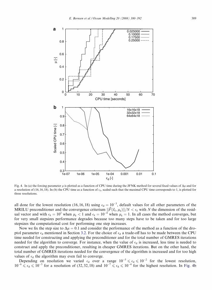
Fig. 4. In (a) the forcing parameter l is plotted as a function of CPU time during the JFNK method for several fixed values of Dl and fora resolution of (16,16,18). In (b) the CPU time as a function of �d, scaled such that the maximal CPU time corresponds to 1, is plotted forthree resolutions.

E. Bernsen et al. / Ocean Modelling 20 (2008) 380–392 389

all done for the lowest resolution (16, 16,18) using �d ¼ 10�3, default values for all other parameters of theMRILU preconditioner and the convergence criterium jj~F ð~xk; lkÞjj=N < �k with N the dimension of the resid-ual vector and with �k ¼ 102 when lk < 1 and �k ¼ 10�4 when lk ¼ 1. In all cases the method converges, butfor very small stepsizes performance degrades because too many steps have to be taken and for too largestepsizes the computational cost for performing one step increases.

Now we fix the step size to Dl ¼ 0:1 and consider the performance of the method as a function of the dro-ptol parameter �d mentioned in Section 3.2. For the choice of �d a trade-off has to be made between the CPUtime needed for constructing and applying the preconditioner and for the total number of GMRES iterationsneeded for the algorithm to converge. For instance, when the value of �d is increased, less time is needed toconstruct and apply the preconditioner, resulting in cheaper GMRES iterations. But on the other hand, thetotal number of GMRES iterations needed for the convergence of the algorithm is increased and for too highvalues of �d the algorithm may even fail to converge.

Depending on resolution we varied �d over a range 10�56 �d 6 10�2 for the lowest resolution,

10�66 �d 6 10�3 for a resolution of (32, 32,18) and 10�7

6 �d 6 10�4 for the highest resolution. In Fig. 4b

0

10

20

30

40

50

60

70

80

90

0 500 1000 1500 2000 2500 3000 3500

Spe

ed-u

p [-

]

Physical time [years]

16x16x1832x32x1864x64x18

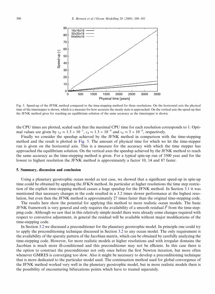
Fig. 5. Speed-up of the JFNK method compared to the time-stepping method for three resolutions. On the horizontal axis the physicaltime of the timestepper is shown, which is a measure for how accurate the steady state is approached. On the vertical axis the speed-up thatthe JFNK method gives for reaching an equilibrium solution of the same accuracy as the timestepper is shown.

390 E. Bernsen et al. / Ocean Modelling 20 (2008) 380–392

the CPU times are plotted, scaled such that the maximal CPU time for each resolution corresponds to 1. Opti-mal values are given by �d � 1:3� 10�3, �d � 1:3� 10�4 and �d � 3� 10�6, respectively.

Finally we consider the speedup achieved by the JFNK method in comparison with the time-steppingmethod and the result is plotted in Fig. 5. The amount of physical time for which we let the time-stepperrun is given on the horizontal axis. This is a measure for the accuracy with which the time stepper hasapproached the equilibrium solution. On the vertical axes the speedup achieved by the JFNK method to reachthe same accuracy as the time-stepping method is given. For a typical spin-up run of 3500 year and for thelowest to highest resolution the JFNK method is approximately a factor 10, 14 and 87 faster.

5. Summary, discussion and conclusion

Using a planetary geostrophic ocean model as test case, we showed that a significant speed-up in spin-uptime could be obtained by applying the JFKN method. In particular at higher resolutions the time step restric-tion of the explicit time-stepping method causes a huge speedup for the JFNK method. In Section 3.1 it wasmentioned that necessary changes in the code resulted in a 3.2 times slower performance at the highest reso-lution, but even then the JFNK method is approximately 27 times faster than the original time-stepping code.

The results here show the potential for applying this method to more realistic ocean models. The basicJFNK framework is very general and only requires the availability of a smooth residual ~F from the time-step-ping code. Although we saw that in this relatively simple model there were already some changes required withrespect to convective adjustment, in general the residual will be available without major modifications of thetime-stepping code.

In Section 3.2 we discussed a preconditioner for the planetary geostrophic model. In principle one could tryto apply the preconditioning technique discussed in Section 3.2 to any ocean model. The only requirement isthe availability of the sparsity pattern of the Jacobian matrix, which can be obtained by carefully analyzing thetime-stepping code. However, for more realistic models at higher resolutions and with irregular domains theJacobian is much more ill-conditioned and this preconditioner may not be efficient. In this case there isthe option to construct the preconditioner not only once before the first Newton iteration, but more oftenwhenever GMRES is converging too slow. Also it might be necessary to develop a preconditioning techniquethat is more dedicated to the particular model used. The continuation method used for global convergence ofthe JFNK method worked very well in the planetary geostrophic model, but in more realistic models there isthe possibility of encountering bifurcations points which have to treated separately.

E. Bernsen et al. / Ocean Modelling 20 (2008) 380–392 391

Another problem not dealt with in the JFNK method is the assumption that a true equilibrium state isreached instead of a statistical equilibrium. In these statistical kind of equilibria the condition (2) does nothold at any point in time, but only in a time averaged sense. One approach of this problem would be to requirethat the time-averaged residual approaches zero, implying that the time-averaged temperature and salinityapproach some constant, and hence we solve, instead of (2), the new time-averaged system ~Gð~xÞ ¼ 0 with~Gð~xÞ ¼ ð1=TÞ

RT

0~F ð~xðtÞÞdt with T an averaging period. However, in this approach the averaging period T

cannot be too long for computational efficiency and a more sophisticated preconditioner has to be used sincethe Jacobian of the new residual ~G may no longer be sparse. Related to the problem of statistical equilibria areperiodic solutions corresponding to a periodic (seasonal) forcing. To find these the approach taken in vanNoorden et al. (2003) can be used.

When applying the JFNK method to realistic ocean models another important issue is how efficient themethod can be implemented on parallel computers. The GMRES method can be parallelized very well andthe same holds for the calculation of the residual ~F , provided that an efficient parallel implementation ofthe original time-stepping code exists. No parallelized version of the MRILU preconditioner exists yet. How-ever, this does not have to be a problem since for more realistic models the preconditioner is likely to bereplaced with a more efficient one anyway.

A comparison of the JFNK method with other acceleration methods is not within the scope of this paper.Our next step is to apply this method to a more realistic ocean model such as POP (Smith and Gent, 2002) orMOM (Griffies et al., 2004) and then make a comparison with other acceleration methods, such as the dis-torted physics method (Bryan, 1984). Some changes in POP or MOM are probably necessary due to therequirement that the residual ~F is smooth. In POP smoothness of the residual with respect to convectiveadjustment is easily obtained since convection is optionally handled by setting jv to high values where staticinstabilities occur, but the use of partial bottom cells potentially causes problems since it results in a non-dif-ferentiable residual. Furthermore the momentum equations in POP are split into a barotropic part, treatedimplicitly and baroclinic part, treated explicitly. Although this splitting makes it harder to extract the residualfrom the time-stepping code directly, it also offers an opportunity to possibly use a physics based precondi-tioner (Nadiga et al., 2006; De Niet et al., 2007).

In conclusion, the method here provides a potentially interesting approach to shorten the spin-up time inlarge-scale ocean models.

References

Botta, E., Wubs, F., 1999. Matrix renumbering ILU: an effective algebraic multilevel ILU preconditioner for sparse matrices. SIAMJournal on Matrix Analysis and Applications 20 (4), 1007–1026.

Bryan, K., 1984. Accelerating the convergence to equilibrium of ocean-climate models. Journal of Physical Oceanography 14, 666–673.

Coleman, T.F., Garbow, B.S., More, J.J., 1984. Software for estimating sparse Jacobian matrices. ACM Transactions on MathematicalSoftware 10 (3), 329–345.

De Niet, A., Wubs, F.W., van Scheltinga, A.D.T., Dijkstra, H.A., 2007. A tailored solver for the bifurcation analysis of ocean-climatemodels. Journal of Computational Physics 227, 654–679.

Dijkstra, H.A., Oksuzo�glu, H., Wubs, F.W., Botta, E.F.F., 2001. A fully implicit model of the three-dimensional thermohaline oceancirculation. Journal of Computational Physics 173, 685–715.

Eisenstat, S.C., Walker, H.F., 1994. Globally convergent inexact Newton methods. SIAM Journal on Optimization 4 (2), 393–422.Fraysse, V., Giraud, L., Gratton, S., Langou, J., 2003. A Set of GMRES Routines for Real and Complex Arithmetics on High

Performance Computers. CERFACS, available on-line at <http://www.cerfacs.fr/algor/reports/2003/TR_PA_03_03.pdf>.Griffies, S., Harrison, M., Pacanowski, R., Rosati, A., 2004. A Technical Guide to MOM4. NOAA/Geophysical Fluid Dynamics

Laboratory, available on-line at <http://www.gfdl.noaa.gov/fms>.Khatiwala, S., Visbeck, M., Cane, M.A., 2005. Accelerated simulation of passive tracers in ocean circulation models. Ocean Modelling 9,

51–69.Klinger, B.A., 2000. Acceleration of general circulation model convergence by exponential extrapolation. Ocean Modelling 2, 61–72.Knoll, D., Keyes, D., 2004. Jacobian–free Newton–Krylov methods: a survey of approaches and applications. Journal of Computational

Physics 193, 357–397.Knoll, D., Mousseau, V., Chacon, L., Reisner, J., 2005. Jacobian–free Newton–Krylov methods for accurate time integration of stiff wave

systems. Journal of Scientific Computing 25 (Nov.), 213–229.Nadiga, B.T., Taylor, M., Lorenz, J., 2006. Ocean modelling for climate studies: eliminating short time scales in long-term, high-resolution

studies of ocean circulation. Mathematical and Computer Modelling 44 (9–10), 870–886.

392 E. Bernsen et al. / Ocean Modelling 20 (2008) 380–392

Reisner, J., Mousseau, V., Knoll, D., 2000. Application of the Newton–Krylov method to geophysical flows. Monthly Weather Review129, 2404–2415.

Reisner, J., Wyszogrodzki, A., Mousseau, V., Knoll, D., 2003. An efficient physics based preconditioner for the fully implicit solution ofsmall-scale thermally driven atmospheric flows. Journal of Computational Physics 189, 30–44.

Saad, Y., 1996. Iterative Methods for Sparse Linear Systems. PWS Publishing Company.Samelson, R., Vallis, G.K., 1995. Planetary-Geostrophic Ocean Model: A User’s Guide. Available on-line at <http://www-po.

coas.oregonstate.edu/homes/rms/ocean/>.Samelson, R., Vallis, G.K., 1997a. Large-scale circulation with small diapycnal diffusion: the two-thermocline limit. Journal of Marine

Research 55, 223–275.Samelson, R., Vallis, G.K., 1997b. A simple friction and diffusion scheme for planetary geostrophic basin models. Journal of Physical

Oceanography 27 (Jan.), 186–194.Smith, R., Gent, P., 2002. Reference Manual for the Parallel Ocean Program (POP). Available on-line at <http://climate.lanl.gov/Models/

POP/POP_Reference.ps>.van Noorden, T., Lunel, S.V., Bliek, A., 2003. The efficient computation of periodic states of cyclically operated chemical precesses. IMA

Journal of Applied Mathematics 68, 149–166.Weijer, W., Dijkstra, H.A., Oksuzoglu, H., Wubs, F.W., De Niet, A.C., 2003. A fully-implicit model of the global ocean circulation.

Journal of Computational Physics 192, 452–470.