University of Groningen

Credit and liquidity risk of banks in stress conditionsEnd, Willem Adrianus van den

IMPORTANT NOTE: You are advised to consult the publisher's version (publisher's PDF) if you wish to cite fromit. Please check the document version below.

Document VersionPublisher's PDF, also known as Version of record

Publication date:2011

Link to publication in University of Groningen/UMCG research database

Citation for published version (APA):End, W. A. V. D. (2011). Credit and liquidity risk of banks in stress conditions: analyses from a macroperspective Groningen: University of Groningen, SOM research school

CopyrightOther than for strictly personal use, it is not permitted to download or to forward/distribute the text or part of it without the consent of theauthor(s) and/or copyright holder(s), unless the work is under an open content license (like Creative Commons).

Take-down policyIf you believe that this document breaches copyright please contact us providing details, and we will remove access to the work immediatelyand investigate your claim.

Downloaded from the University of Groningen/UMCG research database (Pure): http://www.rug.nl/research/portal. For technical reasons thenumber of authors shown on this cover page is limited to 10 maximum.

Download date: 02-06-2018

85

Chapter 6

Liquidity Stress-Tester: A model for stress-testing banks’ liquidity risk

6.1 Introduction

The recent financial crisis has underscored the need to explicitly take into account liquidity risk in

stress-testing frameworks.34 The manifestation of liquidity risk can rapidly move the system into the

tail of the loss distribution through bank runs, the drying up of market liquidity or doubts of

counterparties about banks’ liquidity conditions. In these situations, liquidity can evaporate making a

bank subject to multiple possible equilibria with very different levels of liquidity supply (Banque de

France, 2008). Liquidity risk is not only a source of banks’ funding risk (the ability to raise cash to

fund the assets), but also has a strong link to market liquidity (the ability to convert assets into cash at

a given price). The originate-to-distribute model has made banks increasingly dependent on market

liquidity to secure funding by issuing securities on wholesale markets and by trading credits. As a

result, banks have become more vulnerable to macroeconomic and financial shocks that may engender

liquidity risk.

Various regulatory initiatives in response to the credit crisis have highlighted that banks’

stress-testing practices usually do not incorporate liquidity risk scenarios sufficiently (FSF, 2008).

Banks often underestimate the severity of market-wide stress, such as the disruption of several key

funding markets simultaneously (e.g. repo and securitisation markets). Moreover, banks do not

systematically consider second-order effects that can amplify losses. These can be caused by

idiosyncratic reputation effects and/or collective responses of market participants, leading to

disturbing (endogenous) effects on markets. Banks have insufficient incentives to insure themselves

against such risks. This is because holding liquidity buffers is costly and may create a competitive

disadvantage (FSA, 2007). Besides, liquidity stresses have a very low probability and market

participants could have the perception that central banks will intervene to provide liquidity in stressed

markets.

Macro stress-testing, i.e. testing the financial system as a whole, is an instrument of central

banks and supervisory authorities to assess the impact of market-wide scenarios and possible second

round effects. Such tests with regard to liquidity risk can enhance the insight in the systemic

dimensions of liquidity risk. These exercises can also contribute to market participants’ awareness of

systemic risks. However, liquidity risk is not included in most macro stress-testing models. A main

reason for this is that the multiple dimensions of liquidity risk make quantification difficult (IMF,

34 This chapter is a revised version of Van den End (2010a).

86

2008b). This could also explain the large variation in the extent to which supervisors prescribe limits

on liquidity risk and insurance that banks should hold (BCBS, 2008b).

This chapter presents a stress-testing model which focuses on both market and funding

liquidity risk of banks. Multiple dimensions of liquidity risk are combined into a quantitative measure.

Section 6.2 describes related models by reviewing the literature. Section 6.3 outlines the model

framework of Liquidity Stress-Tester and explains the model structure for the first and second round

effects of shocks to banks’ liquidity. It also provides a parameter sensitivity analysis Section 6.4

presents model simulations for Dutch banks as an illustration, including an anecdotal back test.

Section 6.5 concludes.

6.2 Literature

Our study relates to models of financial intermediation by banks in transmitting and amplifying

shocks. For instance, liquidity risk plays a role in the interaction and contagion between banks in the

interbank market. Upper (2006) presents a survey of interbank contagion models, concentrating on

interbank loans. This channel of contagion is operative when banks become insolvent due to defaults

by their (interbank) counterparties. Contagion may also take the form of deposit withdrawals due to

fears that banks will not be able to meet their liabilities because of losses incurred on their (interbank)

exposures. Upper sees scope for improvements in the specification of the scenarios leading to

contagion. He concludes that a fundamental shortcoming is the absence of behavioural foundations of

the interbank contagion models, which results in the assumption that banks do not react to shocks (i.e.

absence of optimising banks). Adrian and Shin (2008b) add to this that domino models do not take

sufficient account of how prices change. Related to interbank contagion studies is literature that

analyses payment and settlement systems as a potential source of liquidity shocks and contagion

between banks (see, for instance, Leinonen and Soramäki, 2005). Some studies in this field also pay

attention to behavioural reactions (e.g. Bech et al., 2008, Ledruth, 2007).

Recent work provides some more guidance on how micro foundations could be introduced

into financial sector models. In agent based simulation models, market dynamics are driven by

bounded rational, heterogeneous agents using rule of thumbs strategies (Hommes, 2006). A bounded

rational agent behaves under uncertainty and responds to feedbacks in interaction with other agents.

Applied to the financial system, the model of Goodhart et al. (2006) is based on both heterogeneous

banks and households (investors) and operates through endogenous feedback mechanisms, both

amongst banks, investors and between the real and financial sectors. Liquidity indirectly plays a role

through the credit supply of banks to other banks and consumers, while default is endogenous within

the system. A drawback of their model is the simplification of the economy to only banks and

consumers. Furthermore, the authors recognise the challenge of their approach to reflect reality.

87

Aspachs et al. (2006) have calibrated the Goodhart model to values of several banking systems by

using the probability of default of banks as a measure of financial fragility.

Another strand of models links the banking sector to asset markets, which differs from earlier

studies that view liquidity shortages as stemming from the bank’s liability side, due to depositor runs

(e.g. Allen and Gale, 2000) or withdrawals of interbank deposits (Freixas et al., 2000). Von Peter

(2004) relates banks and asset prices in a simple monetary macroeconomic model in which asset

prices affect the banking system indirectly through debtors’ defaults. Asset price movements that are

driven by market liquidity can also lead to endogenous changes in banks’ balance sheets through a

financial accelerator (Adrian and Shin, 2008a). Cifuentes et al. (2005) examine how defaults across

the interbank network are amplified by asset price effects. Herein, market liquidity drives the market

value of banks’ assets which in a downturn can induce sales of assets, depressing prices and inducing

further sales. Nier et al. (2008) apply the same mechanism to an interbank network in which contagion

is dependent on the connectivity, concentration and tiering in the banking sector. In this framework,

the default dynamics with liquidity effects are simulated, including second round defaults of banks.

These result from shocks to the assets of banks, rather than to the liabilities. The model of Diamond

and Rajan (2005) also focuses on the bank’s asset side and shows that a shrinking common pool of

liquidity exacerbates aggregate liquidity shortages. Boss et al. (2006) have developed a system in

which models for market and credit risk are brought together and connected to an interbank network

module. This is similar to the framework developed by Alessandri et al. (2009), which also takes into

account asset-side feedbacks induced by behavioural responses of heterogeneous banks. These two

models are used for stress-testing by the Oesterreichische Nationalbank and the Bank of England,

respectively. Off-balance contingencies are not covered in these models. Feedback effects arising from

market and funding liquidity risk are also (still) missing in most macro stress-testing models of central

banks. Such effects are featuring in models with margin-constrained traders, as in Brunnermeier and

Pedersen (2007). They model two ‘liquidity spirals’, one in which market illiquidity increases funding

constraints through higher margins, and one in which shocks to traders funding contributes to market

illiquidity due to reduced trading positions.

Our approach relates to the last strand of work, but while the study of Brunnermeier and

Pedersen (2009) is mainly conceptual in nature, our model is based on a more mechanical algorithm to

make it operational for simulations with real data. In this respect, the Liquidity Stress-Tester belongs

to the class of simulation models of central banks that are used to quantify the impact of shocks on the

stability of the financial system. The value added of our approach is the focus on the liquidity risk of

banks, taking into account the first and second round (feedback) effects of shocks, including price

effects on markets, induced by behavioural reactions of heterogeneous banks and idiosyncratic

reputation effects. The model centres on the liquidity position of banks and their related risk

management reactions. The contagion channels through which the banks are affected (e.g. the

interbank network, asset markets) are not explicitly modelled. Instead, contagion results from the

88

effects of banks’ reactions on prices and volumes in the markets where other banks are exposed to, as

described in the next section.

6.3 Model

6.3.1 Framework

In stylised form the Liquidity Stress-Tester model can be represented by Figure 6.1. Banks’ liquidity

positions are modelled in three stages: after the first round effects of a scenario, after the mitigating

actions of the banks, and after the second round effects. In each stage, the model generates

distributions of liquidity buffers by bank, including tail outcomes and probabilities of a liquidity

shortfall. The model is driven by Monte Carlo simulations of univariate shocks to market and funding

liquidity risk factors, which are combined into a multifactor scenario. For instance, a credit market

scenario can be assumed to include rising credit spreads, falling market prices of structured credit

securities (market liquidity) and reduced liquidity in the primary markets for debt issues (funding

liquidity). The model is flexible to choose any plausible set of shock events. This deterministic

approach of scenario building is based on economic judgement and historical experiences of

confluences of events that are likely to lead to a banking liquidity crisis. In the model, the scenario

horizon is set at 1 month but the model is flexible to extend it (as an example, Section 6.4.2 presents

outcomes at a horizon of 6 months).

A scenario is uniformly applied to individual banks by weighting the banks’ liquid asset and

liability items (i) that would be affected by the scenario with stress weights (wi). For instance, in case

of the credit market scenario, weights would be attached to banks’ tradable credit portfolios, collateral

values and wholesale funding liabilities. The weights (wi) stand for haircuts in the case of liquid assets

(reflecting reduced liquidity values or mark-to-market losses) and run-off rates in the case of liabilities

(reflecting the drying up of funding). The size of the weights wi differs per balance sheet item

according to the varying sensitivity of assets and liabilities to liquidity stress (see Section 6.3.2).

In the model, a scenario is assumed to unroll in two rounds. In the first round, the initial

effects of shocks to banks’ market and funding liquidity risks are modelled (stage 1 of the model,

represented by the first line of the flow chart in Figure 6.1). This is done by multiplying the liquid

asset and liability items that are affected in the first round of the scenario by the stress weights (wi).

The resulting loss of liquidity is then subtracted from a banks’ initial liquidity buffer. The outcome is

given by ‘liquidity buffer (1)’ in the figure and is in fact a distribution of buffer outcomes per bank,

following from the simulated market and funding liquidity risk events (i.e. the simulated stress

weights, wi).

89

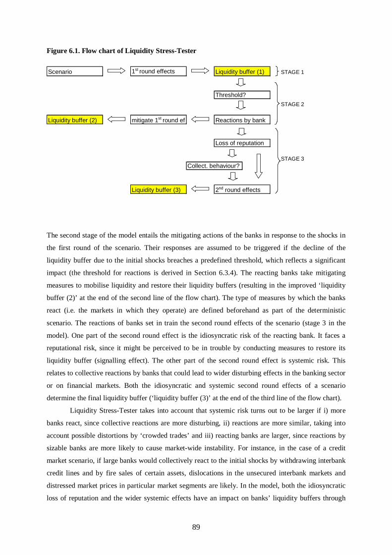
Figure 6.1. Flow chart of Liquidity Stress-Tester

Scenario 1st round effects Liquidity buffer (1) STAGE 1

Threshold?

STAGE 2

Liquidity buffer (2) mitigate 1st round ef Reactions by bank

Loss of reputation

STAGE 3Collect. behaviour?

Liquidity buffer (3) 2nd round effects

The second stage of the model entails the mitigating actions of the banks in response to the shocks in

the first round of the scenario. Their responses are assumed to be triggered if the decline of the

liquidity buffer due to the initial shocks breaches a predefined threshold, which reflects a significant

impact (the threshold for reactions is derived in Section 6.3.4). The reacting banks take mitigating

measures to mobilise liquidity and restore their liquidity buffers (resulting in the improved ‘liquidity

buffer (2)’ at the end of the second line of the flow chart). The type of measures by which the banks

react (i.e. the markets in which they operate) are defined beforehand as part of the deterministic

scenario. The reactions of banks set in train the second round effects of the scenario (stage 3 in the

model). One part of the second round effect is the idiosyncratic risk of the reacting bank. It faces a

reputational risk, since it might be perceived to be in trouble by conducting measures to restore its

liquidity buffer (signalling effect). The other part of the second round effect is systemic risk. This

relates to collective reactions by banks that could lead to wider disturbing effects in the banking sector

or on financial markets. Both the idiosyncratic and systemic second round effects of a scenario

determine the final liquidity buffer (‘liquidity buffer (3)’ at the end of the third line of the flow chart).

Liquidity Stress-Tester takes into account that systemic risk turns out to be larger if i) more

banks react, since collective reactions are more disturbing, ii) reactions are more similar, taking into

account possible distortions by ‘crowded trades’ and iii) reacting banks are larger, since reactions by

sizable banks are more likely to cause market-wide instability. For instance, in the case of a credit

market scenario, if large banks would collectively react to the initial shocks by withdrawing interbank

credit lines and by fire sales of certain assets, dislocations in the unsecured interbank markets and

distressed market prices in particular market segments are likely. In the model, both the idiosyncratic

loss of reputation and the wider systemic effects have an impact on banks’ liquidity buffers through

90

additional haircuts on liquid assets and withdrawals of liquid liabilities (i.e. the second round effects

further increase the stress weights, wi of the affected balance sheet items).

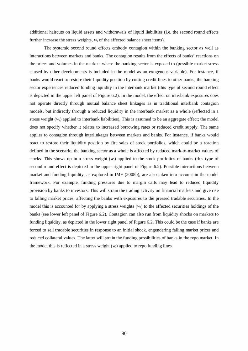
The systemic second round effects embody contagion within the banking sector as well as

interactions between markets and banks. The contagion results from the effects of banks’ reactions on

the prices and volumes in the markets where the banking sector is exposed to (possible market stress

caused by other developments is included in the model as an exogenous variable). For instance, if

banks would react to restore their liquidity position by cutting credit lines to other banks, the banking

sector experiences reduced funding liquidity in the interbank market (this type of second round effect

is depicted in the upper left panel of Figure 6.2). In the model, the effect on interbank exposures does

not operate directly through mutual balance sheet linkages as in traditional interbank contagion

models, but indirectly through a reduced liquidity in the interbank market as a whole (reflected in a

stress weight (wi) applied to interbank liabilities). This is assumed to be an aggregate effect; the model

does not specify whether it relates to increased borrowing rates or reduced credit supply. The same

applies to contagion through interlinkages between markets and banks. For instance, if banks would

react to restore their liquidity position by fire sales of stock portfolios, which could be a reaction

defined in the scenario, the banking sector as a whole is affected by reduced mark-to-market values of

stocks. This shows up in a stress weight (wi) applied to the stock portfolios of banks (this type of

second round effect is depicted in the upper right panel of Figure 6.2). Possible interactions between

market and funding liquidity, as explored in IMF (2008b), are also taken into account in the model

framework. For example, funding pressures due to margin calls may lead to reduced liquidity

provision by banks to investors. This will strain the trading activity on financial markets and give rise

to falling market prices, affecting the banks with exposures to the pressed tradable securities. In the

model this is accounted for by applying a stress weights (wi) to the affected securities holdings of the

banks (see lower left panel of Figure 6.2). Contagion can also run from liquidity shocks on markets to

funding liquidity, as depicted in the lower right panel of Figure 6.2. This could be the case if banks are

forced to sell tradable securities in response to an initial shock, engendering falling market prices and

reduced collateral values. The latter will strain the funding possibilities of banks in the repo market. In

the model this is reflected in a stress weight (wi) applied to repo funding lines.

91

Figure 6.2. Systemic effects through contagion channels

Interbank contagion Contagion through asset markets

Reacting banks Total banking sector Reacting banks Total banking sectorinterbank interbank fire sales value stock

lending ↓ funding ↓ stocks ↓ portfolios ↓

From funding to market liquidity From market to funding liquidity

Reacting banks Total banking sector Reacting banks Total banking sectorliquidity margin calls value tradable fire sales MtM loss securedprovision ↓ securities ↓ securities ↓ collateral ↓ funding ↓

6.3.2 Data

Although Liquidity Stress-Tester is a top-down model, it is run with bank level data. We use the

liquidity positions (both liquid stocks or non-calendar items and cash flows or calendar items) of the

Dutch banks, that are available from De Nederlandsche Bank’s (DNB’s) (2003) liquidity report. It

contains end of month data, which are available since 2003. Data are provided by all Dutch banks (85

on average, including branches and subsidiaries of foreign banks) and cover liquid assets and

liabilities, scheduled payments and on and off-balance sheet items, with a detailed break-down per

balance sheet item. Appendix 2.1 in Chapter 2 provides an overview of the items in the report. Not all

items are reported by all banks, since most do not have exposures to all categories. The average

granularity reported per bank is around 7 items; the large banks report more items, owing to their more

diversified businesses. The top 5 banks, which cover around 85% of the Dutch sector, have an average

granularity of 54 items.

The baseline is a going concern situation, as reflected in unweighted liquid assets and

liabilities. This assumes that liabilities can be fully refinanced and that the liquidity value of assets is

100%, i.e. the weights (wi) are 0. The weights are taken from DNB’s liquidity report (DNB, 2003). In

the report, the actual liquidity of a bank must exceed the required liquidity, at both a one week and a 1

month horizon. By this, the report tends to focus not only on the very short term, but also on the more

structural liquidity position of banks. In the report, actual liquidity is defined as the stock of liquid

assets (weighted for haircuts) and the cash inflow (weighted for their liquidity value) during the test

92

period. Required liquidity is defined as the assumed calls on contingent liquidity lines, assumed

withdrawals of deposits, drying up of wholesale funding and liabilities due to derivatives. In this way,

the liquidity report comprises a combined stock and cash flow approach. The weights (wi) applied to

the liquid assets and liabilities in the DNB report represent a mix of a firm specific and market wide

scenario and are based on best practices and values of haircuts on liquid assets and withdrawal or run-

off rates of liabilities typically used by the industry and rating agencies.35 This makes them a useful

point of departure for our model. The parameterisation of the run-off rates, either based on best

practices or historical data, is a weakness in most liquidity stress-testing models of banks. This is

because data of stress situations are scarcely available and in times of stress the assumed elasticities

may behave differently. As a consequence, banks may underestimate the stability of their funding

base. By applying a stochastic approach, Liquidity Stress-Tester takes into account this uncertainty of

the model parameters.

6.3.3 First round effects

In Liquidity Stress-Tester the fixed weights of DNB’s liquidity report are assumed to be 0.1% tail

events (wi ≈ 3σ).36 The scenario impact of the first round effect on an item i is determined by simulated

weights (w_sim1,i). These are based on Monte Carlo simulations by taking random draws from a log-

normal distribution Log-N (0,1), scaled by (3

LCR wi ), so that wi sim1 ~ Log-N (µ,σ2). The use of a log-

normal distribution is motivated by the typical non-linear features of extreme liquidity stress events.

The log-normal distribution, which is skewed to the right, captures this feature. Its asymmetric shape

fits well on financial market data in particular in high volatility regimes. For that reason the log-

normality of asset returns plays an important role in theory of risk management and asset pricing

models. Besides, the log-normal distribution is bounded below by 0 which is also due for the

simulated weights in our model. As an upper bound, the weights are truncated at w_sim1,i ≤ 100 in the

simulations, since haircuts and withdrawal rates cannot exceed 100%. This procedure delivers a log-

normal distribution of weights which is bounded below by 0 and truncated at the top by 100. The

liquidity buffer in the baseline situation (normal market conditions), B0, is

∑=

−=nc

1i

b

i,calnon

b

0IB (6.1)

b being the individual bank and Inon-cal, i the amount of available assets of non-calendar items (the stock

items of liquid assets 1 .. nc). By this, the buffer consists of deposits at the central bank, securities that

35 In the model, the weights of DNB’s liquidity report that apply to a horizon of 1 month are used. The liquidity model of Standard & Poor’s (2007) is based on a standard set of assumptions, i.e. a spectrum of asset haircuts and liability run-off rates, that were established after a review of bank balance sheets, industry, S&P data and dialogue with risk managers. 36 In the model simulations this assumption could be changed according to other insights.

93

can be turned into cash at short notice, ECB eligible collateral, interbank assets available on demand

and receivables from other professional money market players available on demand. B0 provides

counterbalancing capacity to liquidity scenarios in which liquidity values of the stock of assets could

decline and a drain of liquidity could occur due to decreasing net outflows of liquidity. This means

that the scenario effects could be felt through both deteriorating liquid stocks and flows. The first

round effect (E1) of the scenario is determined by,

i,i

bi

b sim_wIE 11 ∑= (6.2)

I i being the amount of all liquid (non-calendar and calendar) asset and liability items. The liquidity

buffer after the first round impact of the scenario, B1, is,

b

1

b

0

b

1EBB −= (6.3)

6.3.4 Banks’ response to scenario (mitigating actions)

Banks that are affected seriously by the first round effects of the scenario are assumed to restore their

liquidity buffer to the initial level (B0). Banks may take actions to safeguard their stability and/or to

meet liquidity risk criteria of supervisors and rating agencies. In the model, the trigger for a bank’s

reaction is a decline of its original liquidity buffer that exceeds a threshold θ. By this, reactions are

triggered by a significantly large impact of the first round of the scenario (as reflected in the simulated

buffer B1). The trigger q (0, 1) is based on a probability condition (probit),

with q =

>

otherwise0B

Eif1

b

o

b

1 θ

The latent variable θ can be seen as a ‘rule measure’ which banks follow due to self imposed liquidity

risk controls or regulatory requirements. The rule is operationalised by assuming that large value

change of balance sheet items reflect banks’ intentional responses to a buffer decline. The rule variable

θ can then be derived from the average correlation between value changes of balance sheet items and

declines of liquidity buffers one month lagged:

)I

II,

B

BB(Correl

b

0t,i

b

0t,i

b

1t,i

b

1t

b

1t

b

0t

=

==

−=

−==−− , conditioned by

0B

BBb

1t

b

1t

b

0t <−

−=

−==

The lag controls for the influence of possible endogeneity in the relationship between the buffers and

the balance sheet items. In an empirical application for the Dutch banking sector the correlation

94

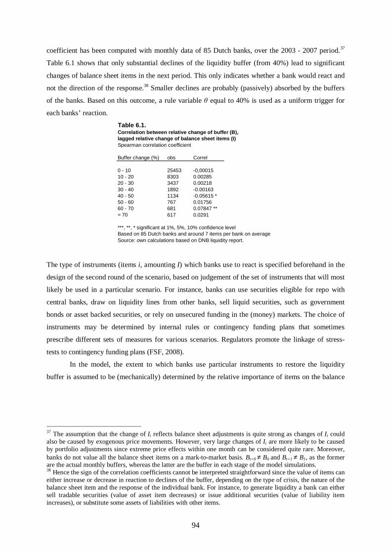
coefficient has been computed with monthly data of 85 Dutch banks, over the 2003 - 2007 period.37

Table 6.1 shows that only substantial declines of the liquidity buffer (from 40%) lead to significant

changes of balance sheet items in the next period. This only indicates whether a bank would react and

not the direction of the response.38 Smaller declines are probably (passively) absorbed by the buffers

of the banks. Based on this outcome, a rule variable θ equal to 40% is used as a uniform trigger for

each banks’ reaction.

Table 6.1.Correlation between relative change of buffer (B), lagged relative change of balance sheet items (I)Spearman correlation coefficient

Buffer change (%) obs Correl

0 - 10 25453 -0,0001510 - 20 8303 0.0028520 - 30 3437 0.0021830 - 40 1892 -0.0016340 - 50 1134 -0.05615 *50 - 60 767 0.0175660 - 70 681 0.07847 **= 70 617 0.0291

***, **, * significant at 1%, 5%, 10% confidence levelBased on 85 Dutch banks and around 7 items per bank on averageSource: own calculations based on DNB liquidity report.

The type of instruments (items i, amounting I) which banks use to react is specified beforehand in the

design of the second round of the scenario, based on judgement of the set of instruments that will most

likely be used in a particular scenario. For instance, banks can use securities eligible for repo with

central banks, draw on liquidity lines from other banks, sell liquid securities, such as government

bonds or asset backed securities, or rely on unsecured funding in the (money) markets. The choice of

instruments may be determined by internal rules or contingency funding plans that sometimes

prescribe different sets of measures for various scenarios. Regulators promote the linkage of stress-

tests to contingency funding plans (FSF, 2008).

In the model, the extent to which banks use particular instruments to restore the liquidity

buffer is assumed to be (mechanically) determined by the relative importance of items on the balance

37 The assumption that the change of I i reflects balance sheet adjustments is quite strong as changes of I i could also be caused by exogenous price movements. However, very large changes of I i are more likely to be caused by portfolio adjustments since extreme price effects within one month can be considered quite rare. Moreover, banks do not value all the balance sheet items on a mark-to-market basis. Bt=0 ≠ B0 and Bt=1 ≠ B1, as the former are the actual monthly buffers, whereas the latter are the buffer in each stage of the model simulations. 38 Hence the sign of the correlation coefficients cannot be interpreted straightforward since the value of items can either increase or decrease in reaction to declines of the buffer, depending on the type of crisis, the nature of the balance sheet item and the response of the individual bank. For instance, to generate liquidity a bank can either sell tradable securities (value of asset item decreases) or issue additional securities (value of liability item increases), or substitute some assets of liabilities with other items.

95

sheet (

∑i

bi

bi

I

I ), reflecting a bank’s specialisation and presence in certain markets.39 Since in liquidity

crises, time is usually very short and banks often do not have the opportunity to change their strategy

(e.g. by diversifying funding or spreading risk). The size of the transactions that a bank conducts with

instrument i is expressed by b

iRI ,

)I

I()BB(RI

i

bi

bibbb

i∑

−= 10 (6.4)

Since B1 ≤ B0, by definition b

iRI is positive. This does not imply anything about the direction of the

transaction (e.g. buying or selling) but it indicates the (absolute) size of the transaction that is needed

to generate liquidity ( b

iRI is a size factor). Hence, the liquidity buffer after the mitigating actions (B2)

of a bank is equal to,

)sim_w(RIBB i,i

bi

bb112 100−+= ∑ (6.5)

with B2 > B1, but B2 < B0, since the buffer cannot be fully restored due to the market disturbances in

the first round of the scenario (as reflected in w_sim1,i). In an extreme stress situation, financial

markets may be gridlocked completely due to the drying up of liquidity. Such an extreme case is

represented by w_sim1,i = 100, implying that banks have no possibility to enter a particular market

segment to raise additional liquidity. In the case of the repo markets this could mean that certain

collateral of banks may be useless.

6.3.5 Second round effects

The behavioural reactions of the banks can have wider disturbing (endogenous) effects on markets,

feeding back on the banks. This will be manifested in additional haircuts on liquid assets and

withdrawals of liquid liabilities in the market segments where banks react, as reflected in w_sim2,i

(with w_sim1,i ≤ w_sim2,i ≤ 100). The feedback effects are larger if more banks react (∑b

q) and if

reactions are similar, which is expressed by the sum of reactions by a particular instrument (∑b

b

iRI ).

This summation is divided by the total amount of reactions )RI(i b

b

i∑∑ to get the ratio that indicates

the similarity of reactions (

∑∑

∑

i b

bi

b

bi

RI

RI ). In the case of deep and liquid markets (e.g. the government bond

market) where discretionary transactions will have little effects, w_sim2,i is smaller than in the case of

39 The model does not specify the conditions (e.g. credit spreads) at which funding is attracted.

96

illiquid market segments. Such differences will already be reflected in w_sim1,i from which w_sim2,i is

derived,

∑=

∑∑∑

∑+

b

b

s)RI

RI(

i,i, q

q

sim_wsim_w

i b

b

i

b

b

i

1

12 (6.6)

Since b

iRI indicates the size of the transaction that is conducted to generate liquidity, higher values of

b

iRI imply a higher liquidity demand, which will adversely affect the availability of liquidity in market

segments in which the banks operate. By including RIi in equation 6.6, large transactions have more

impact on markets than small transactions. This implicitly means that reactions by large banks induce

stronger second round effects than reactions by small banks.40 Variable s is a state variable which

represents the exogenous market conditions. Equation 6.6 has parallels with the asset price function

used by Alessandri et al., 2009 and Nier el al., 2008. In their models, the price of banking assets is a

decreasing function of the amount of assets sold by banks, while the price also depends on market

liquidity.

More in particular, the state variable s represents an indicator of exogenous market stress. The

ranges of this variable are derived from standardised distributions of risk aversion indicators. For this

the implied stock price volatility (VIX index) and the US corporate bond spreads (Baa) were used as

proxies. Figures 6.3a and 6.3b show standardised frequency distributions of these series. To determine

a range of s for use in the model, we assume that normal market conditions are reflected by -1 ≤ s ≤ 1

(which according to a standardised distribution of risk indicators, represents 2/3 of market conditions)

and severe market stress by s = 3 (i.e. 0.5% of adverse market situations). s could be even higher, as

panels A and B in Figure 6.3 indicate. For the purpose of measuring liquidity stress in the model, the

restriction s ≥ 1 applies. The risk aversion indicators could be used to conduct periodic runs with

Liquidity Stress-Tester in which changing market conditions play a role.

Figure 6.3. Frequency distribution of risk aversion indicators

0%

10%

20%

30%

40%

50%

-3 -2 -1 0 1 2 3 More

Panel B. Frequency distribution of implied volatilityNormalised value of S&P500 stock price volatility (VIX index), daily data period 1986-2007

Source of VIX: Chicago Board Option Exchange

0%

10%

20%

30%

40%

50%

-3 -2 -1 0 1 2 3 More

Panel A. Frequency distribution of credit spreadsNormalised value of Moodys Baa average credit spreads on corporate bonds, daily data period 1986-2007

Source credit spreads: US Federal Reserve 40 By running Liquidity Stress-Tester with a limited sample of banks (in this chapter the Dutch banks) it is implicitly assumed that the reactions of this sample are representative for the (global) banking system as a whole.

97

In the model, the market conditions contribute to the severity of the second round effects: the higher is

s, the stronger are the effects of the number and the similarity of banks’ reactions. In that respect, the

fall-out of the market stress (reflected in s) differs for each market segment. We do not model

feedback effects running from banks’ reactions to s, assuming that the market stress represents an

exogenous shock that drives the reactions by banks. Endogenising variable s, by making it dependent

on banks’ reactions, would complicate the model by introducing a circular reference. Conducting

periodic model runs with a time variant value of s will solve this to some extent, since market wide

risk aversion indicators will reflect the influence of banks’ reactions on market conditions.

Panels A and B in Figure 6.4 illustrate the relationship between w_sim2,i and w_sim1,i and its

dependence on the number of reacting banks (∑b

q ), the similarity of reactions (

∑∑

∑

i b

bi

b

bi

RI

RI ) and the level

of market stress (s). It is assumed that the similarity of reactions has a stronger effect on markets than

the number of reacting banks (see the exponential relationship in panel B). The intuition behind is that

the similarity of reactions points to crowded trades in markets which cause a drying up of market

liquidity.

Banks that react in order to restore their liquidity buffer face a reputation risk in the financial markets.

While applying sensible measures ought to strengthen a banks’ financial position and comfort

counterparties, the adverse signalling effect of the transactions could reverberate on the conditions that

banks face in the markets. This could translate in even more (idiosyncratic) haircuts on liquid assets

and withdrawals of liquid liabilities, as reflected in w_sim*2,i (with w_sim2,i ≤ w_sim*2,i ≤ 100). The

reputation effect will depend on the market conditions (s) driving the second round effects, since

particularly in stressed circumstances the signalling effect of reactions will adversely feedback on a

98

bank (the stigma associated with accessing central bank standing facilities in the recent crisis is

illustrative).41 In functional form, the reputation risk is expressed by,

ssim_wsim_w i,*

i, 22 = (6.7)

Next, the additional impact of the (systemic and idiosyncratic) second round effects on banks is

determined by E2,

))sim_wsim_w()RII((E i,i

i,bi

bi

b122 ∑ −+= (6.8)

with w_sim2,i being replaced by w_sim*2,i in case a reacting bank also faces reputation risk. The

liquidity buffer after the second round effects (B3) is,

b

2

b

2

b

3EBB −= (6.9)

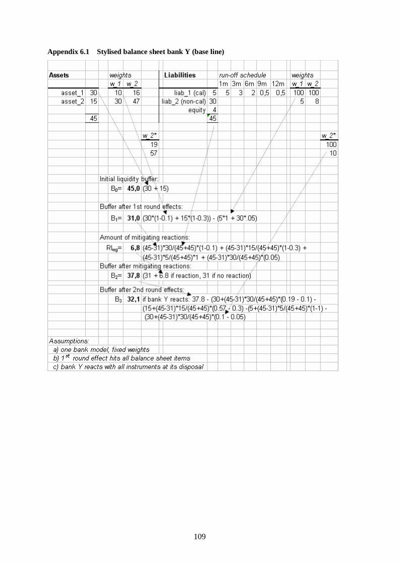
6.3.6 Impact different scenario rounds

The stylised balance sheet in Appendix 6.1 shows how the model works in a simplified one bank

situation. A hypothetical scenario is assumed to affect all liquid assets and liabilities of the bank

through fixed in stead of simulated stressed weights. Furthermore, it is assumed that the first round

effect of the scenario leads to a decline of the initial liquidity buffer that exceeds the threshold θ and

that the bank reacts with all instruments available at its disposal (i.e. asset items 1 and 2 and liability

items 1 and 2 on the stylised balance sheet). This example shows that the mitigating actions of the

bank improves its liquidity buffer (to B2), although it remains below the initial level (B0). The second

round effects reduce the buffer further (to B3), below the level after the first round shock (B1).

In the stochastic mode of the model, each round of a scenario has its typical effect on the

distribution of buffer outcomes. Simulations with real bank data show that the first round effect leads

to a shift of the distribution to the left (B1), while the mitigating actions shift the distribution (B2) back

towards B0 and cause a peakening of the shape (panel B in Figure 6.5)42. If a bank does not react

because θ<0

1

B

E , the distributions of B1 and B2 coincide. This is the case with bank AH in panel A of

Figure 6.5. The second round effect shifts the distribution (B3) to the left again and causes a flattening

of the distribution. The average of this final distribution (3B ) is substantially smaller than 1B , which

indicates that the second round effects outweigh the initial shock. Such an outcome is conceptually

explained by Nikolaou (2009). For a bank which does not face a reputation risk the second round

41 Equation 6.7 has been calibrated on the actual outcomes of the individual banks and on the share of the reputational effect in the total second round effect (see Section 6.4). If s = 1 (the downside restriction for s), than the mitigating reaction of a bank will not be counteracted by adverse reputational effects and will improve a banks’ liquidity position by definition. 42 The parameters of these simulations are equal to those applied in Section 6.4.

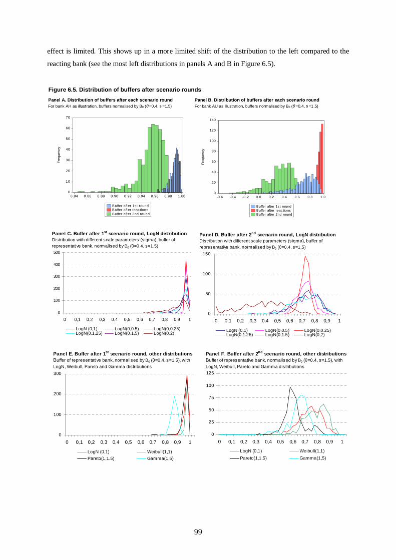
99

effect is limited. This shows up in a more limited shift of the distribution to the left compared to the

reacting bank (see the most left distributions in panels A and B in Figure 6.5).

Figure 6.5. Distribution of buffers after scenario rounds

Panel A. Distribution of buffers after each scenario round Panel B. Distribution of buffers after each scenario roundFor bank AH as illustration, buffers normalised by B0 (θ=0.4, s =1.5) For bank AU as illustration, buffers normalised by B0 (θ=0.4, s =1.5)

0

20

40

60

80

100

120

140

-0.6 -0.4 -0.2 0.0 0.2 0.4 0.6 0.8 1.0

Buffer after 1st roundBuffer after reactionsBuffer after 2nd round

Fre

quen

cy

0

10

20

30

40

50

60

70

0.84 0.86 0.88 0.90 0.92 0.94 0.96 0.98 1.00

B uffer after 1st roundB uffer after reac tionsB uffer after 2nd round

Fre

que

ncy

0

100

200

300

400

500

0 0,1 0,2 0,3 0,4 0,5 0,6 0,7 0,8 0,9 1

LogN (0,1) LogN(0,0.5) LogN(0,0.25)LogN(0,1.25) LogN(0,1.5) LogN(0,2)

Panel C. Buffer after 1st scenario round, LogN distributionDistribution with different scale parameters (sigma), buffer of representative bank, normalised by B0 (θ=0.4, s=1.5)

0

50

100

150

0 0,1 0,2 0,3 0,4 0,5 0,6 0,7 0,8 0,9 1

LogN (0,1) LogN(0,0.5) LogN(0,0.25)LogN(0,1.25) LogN(0,1.5) LogN(0,2)

Panel D. Buffer after 2nd scenario round, LogN distributionDistribution with different scale parameters (sigma), buffer of representative bank, normalised by B0 (θ=0.4, s=1.5)

0

25

50

75

100

125

0 0,1 0,2 0,3 0,4 0,5 0,6 0,7 0,8 0,9 1

LogN (0,1) Weibull(1,1)

Pareto(1,1.5) Gamma(1,5)

Panel F. Buffer after 2nd scenario round, other distributionsBuffer of representative bank, normalised by B0 (θ=0.4, s=1.5), with LogN, Weibull, Pareto and Gamma distributions

0

100

200

300

0 0,1 0,2 0,3 0,4 0,5 0,6 0,7 0,8 0,9 1

LogN (0,1) Weibull(1,1)

Pareto(1,1.5) Gamma(1,5)

Panel E. Buffer after 1st scenario round, other distributionsBuffer of representative bank, normalised by B0 (θ=0.4, s=1.5), with LogN, Weibull, Pareto and Gamma distributions

100

6.3.7 Influence of alternative distributional assumptions

As explained in Section 6.3.3 the simulated weights are based on a log-normal distribution Log-N

(0,1). The choice of a probability distribution function for non-negative random variables is motivated

by the need to produce weights that are bounded below by 0. This lower bound explains the location

parameter µ =0, which reflects normal market conditions (no stress). The scale parameter σ =1 is used

to scale the weights by (3

LCR wi ). To test the sensitivity of the model for alternative distributional

assumptions, the scale parameter (σ) is varied between 0.25 and 2. Panels C and D in Figure 6.5 show

the resulting distributions of the liquidity buffer of a representative bank after the first and second

rounds of a hypothetical scenario. It appears that the simulation outcomes are quite robust to different

values of the scale parameter, in particular with regard to the first round effects presented in panel C.

The scale parameter has more influence on the second round effects as presented in panel D. A higher

value of σ leads to a flattening of the buffer distribution, which becomes very pronounced at σ =2.

Next to the log-normal distribution, other distributions as well exhibit the features that are

desirable for our model, such as being skewed to the right. Hence, as another sensitivity test, different

distributional forms are used to generate buffer outcomes of a hypothetical scenario. Panels E and F in

Figure 6.5 show the liquidity buffers of a representative bank after the first and second rounds of a

hypothetical scenario, based on the log-normal, Gamma, Weibull and Pareto distributions. It appears

that the first round effects presented in panel E are quite robust to different distributional forms (only

the Gamma distribution generates outcomes that are located more to the left). The distributional form

has more substantial influence on the second round effects as presented in panel F (of course the

location and shape of the distributions depend on the choice of the moments for each distribution). The

simulation outcomes based on the log-normal and Weibull distributions are quite similar, but the use

of the Gamma and Pareto distributions changes the outcomes significantly. This highlights the

importance of the choice for a distributional form, which for our model is motivated in Section 6.3.3.

In extreme value theory (EVT) the Gumbel, Frechet and Weibull distributions are used (Poon et al.,

2004). This class of distributions provides for a non-degenerate limit as n → ∞, which is the desired

feature for estimates of tail values beyond a certain cut-off point. EVT focuses on the tail of the

distribution and only uses data from the tail area to model that part of the distribution. Thereby it

differs from our approach, as the Liquidity Stress-Tester model simulates the full range of buffer

outcomes.

6.3.8 Parameter sensitivity

Based on the same stylised balance sheet in Appendix 6.1, this section exposes the sensitivity of the

outcomes for changing the model parameters. In the base line situation, the level of market stress (s) is

101

set at 1.5, the number of reacting banks (∑b

q ) at 2, the similarity of reactions (

∑∑

∑

i b

bi

b

bi

RI

RI ) at 0.05 and

the scenario horizon at 1 month. Table 6.2 shows the impact of changing each parameter in isolation

on the banks’ liquidity buffer, in terms of deviations of the final buffer (B3) from the initial buffer (B0).

At first sight the model outcomes look relatively sensitive to changes of s (the buffer declines by

nearly 2/3 if s = 3) and less to changes in the number of reacting banks and the similarity of reactions

(the sensitivity analysis affirms that the latter has a stronger effect on markets than the number of

reacting banks). As explained in Section 6.3.5, s reinforces the effects of the number of reacting banks

and the similarity of reactions and these factors can hardly be assessed in isolation. Following from

equation 6.7, the impact of reputational risk (due when banks respond to a scenario by mitigating

actions) also depends on the level of market stress. Table 6.2 shows that reputational risk could

severely impact on banks in stressed markets. The model outcomes are also quite sensitive to

lengthening the scenario horizon; the final buffer declines by ¼ if the horizon is lengthened from 1 to

12 months (which includes the total run-off schedule of liability 1, which is a calendar item).

102

6.4 Results

This section describes model outcomes by simulating a hypothetical scenario (a ‘classical’ banking

crisis), and an historical scenario (the recent credit market crisis). These scenarios are run with July

2007 data of all banks in the Netherlands (including subsidiaries of foreign banks).43 The model

outcomes are based on 500 Monte Carlo simulations. In first instance we assume θ = 0.4 (the critical

threshold determined in Section 6.3.4), s = 1.5 (the middle of the range determined in Section 6.3.544)

and a horizon of one month (typically used in banks’ liquidity stress-tests). These values are used in

the simulations, but can be adjusted to other circumstances (as illustrated in Section 6.4.3).

Experimenting with the parameter values enhances the insight in the sensitivity of the model outcomes

for banks’ reactions, the level of market stress and the length of the scenario horizon.

6.4.1 Banking crisis scenario

The first round of the hypothetical banking crisis scenario seizes at the liability side of banks’ balance

sheets. It assumes a public crisis of confidence affecting the banking sector, which could result from

massive misselling of a financial product in the retail market. This scenario leads to a withdrawal of

non-bank deposits and other funding by professional money market players, other institutional

investors and corporates and by withdrawals of savings deposits by households. These first round

effects are simulated by stressing the weights of the affected deposits and funding sources (through

w_sim1,i). These weights determine the first round effect (E1) according to equation 6.2 and the

liquidity buffer (B1) according to equation 6.3. Table 6.3 shows the average outcomes for all banks.

On average, the first round effect erases 8% of the initial liquidity buffer. Some small banks would be

faced with a negative liquidity buffer after the first round of the scenario.

Table 6.3 shows that for 30 banks the decline of the liquidity buffer exceeds the threshold θ =

0.4 which triggers them to restore their liquidity buffer to the initial level (B0).45 The reactions mitigate

the first round effect of the scenario on the sector as a whole to around 7% on average (B2 being 0.5%

smaller than B0). Panel A.3 in Appendix 6.2 indicates that smaller banks tend to react relatively more

than large banks, which indicates that an outflow of deposits would foremost bring small banks in a

critical liquidity position.

In the second round of the scenario, it is assumed that banks react to the funding pressures by

drawing upon credit lines in the unsecured interbank market. These mitigating actions can be an

important source of feedback effects among banks. They are interdependent via interbank liquidity

43 In July 2007 the number of banks included in the data was 82 (on average, since 2003, 85 banks have been included in the dataset). 44 Note that at mid December 2007 during a height of the credit crisis, s was around 1 based on corporate bond spreads and around 0.5 based on implied stock price volatility. 45 The table reports the averages of the simulated buffers, whereas the reactions are triggered by extreme downward changes in the simulated sample of buffers.

103

promises and widespread use of these lines will lead to contagion of liquidity risk. The feedback

effects (w_sim2,i) are simulated by stressing the weights of the unsecured interbank assets and

liabilities. Next to these systemic second round effects, the banks which react by drawing upon

liquidity promises of counterparties face a reputation risk since their actions could be perceived as a

sign of weakness. In the model simulations this translates into additional (idiosyncratic) stress on the

weights (w_sim*2,i) according to equation 6.7. Both the reputational risk and the systemic (second

round) effects on the markets have an impact on the liquidity buffers of the banks (E2) according to

equation 6.8 and on the final liquidity buffer (B3) according to equation 6.9. Table 6.3 shows that due

to the second round effects the banks additionally loose 6% of their initial liquidity buffers on average

(including the effects of mitigation actions). Table 6.3 also shows the 5% and 1% tail outcomes of the

final liquidity buffer and the probability of a liquidity shortfall (i.e. B3 < 0). Insight in the extreme tail

outcomes is particularly relevant for financial stability analysis which assesses the resilience of the

system to extreme, but plausible shocks. In the 5% (1%) tail the liquidity buffer declines by 26%

(32%) on average. Out of the total sample, 25 banks have a probability larger than 0% to end up with a

liquidity shortage. These are mostly small banks which explains that the (by the initial liquidity buffer)

weighted average probability of a liquidity shortfall is limited to 0.5%. The latter is an indicator of the

liquidity risk of the financial system as a whole. Panel A.5 in Appendix 6.2 indicates a significant

negative correlation between the shortfall probability and size of banks, which affirms that small

banks are most vulnerable to a ‘classical’ banking crisis scenario.

6.4.2 Credit crisis scenario

The first round of the credit crisis scenario seizes at the asset side of banks’ balance sheets. It is

designed by assuming declining values of banks’ tradable credit portfolios, due to uncertainties about

the asset valuations which cause a drying up of market liquidity. The falling collateral values lead to

higher margin requirements on banks’ derivative positions. These first round effects are simulated by

stressing the weights of the credit portfolios and margin requirements (through w_sim1,i). Table 6.3

shows the average outcome for all banks. The first round effect erases 13% of the initial liquidity

buffer, with a maximum of 92% for the bank that is most severely affected. Although most banks

would be affected by the scenario (i.e. b

0

b

1BB < ), the liquidity buffers of the affected banks remain in

surplus in all cases. The banks that are not affected at this stage of the scenario are mostly small

branches of foreign banks. They can count on liquidity support from the head office and probably

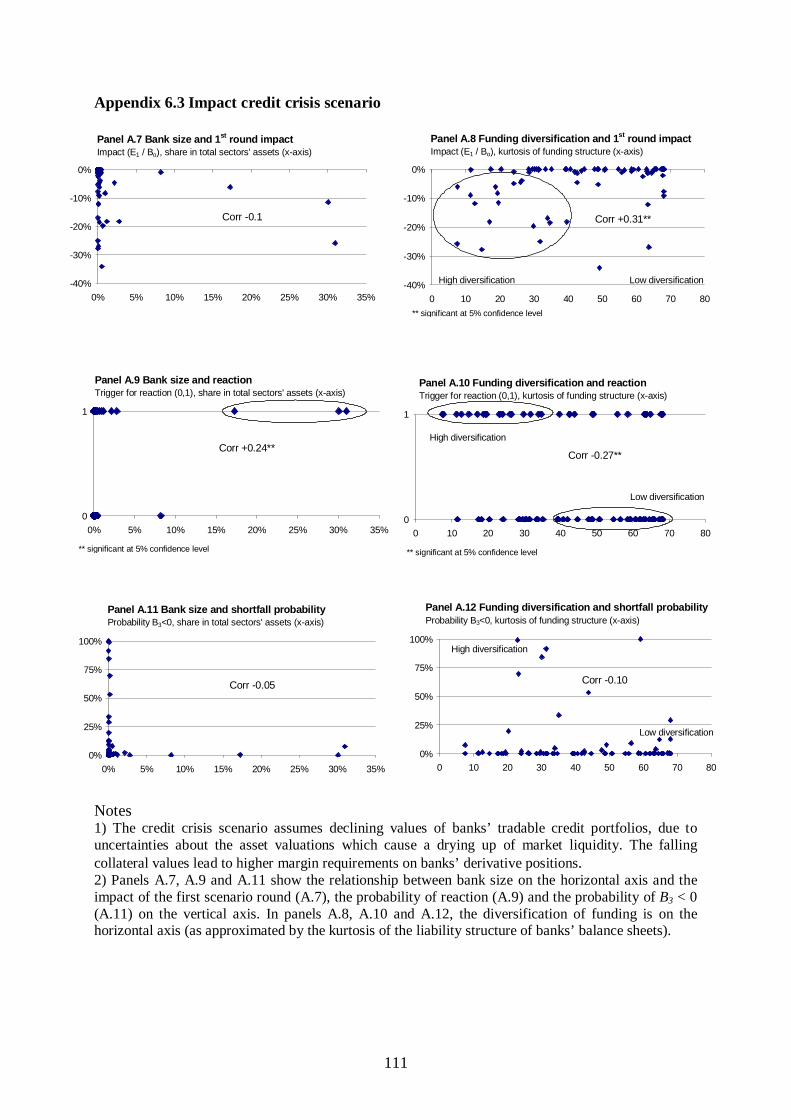
therefore do not hold eligible collateral. A break-down of the sample by bank size and funding

structure indicates that banks with a more diversified funding profile are relatively more vulnerable to

the first round of the scenario (see panel A.8 in Appendix 6.3; panel A.7 indicates that there is no

significant correlation with bank size). Although a more diversified funding profile in general

improves banks’ resilience to liquidity shocks, the fact that the recent crisis has been most felt in

104

international financial markets has raised the vulnerability of banks that rely on wholesale funding,

next to retail deposits. This underscores that liquidity risk management should identify and measure

the full range of liquidity risks which banks face.

Table 6.3 shows that in case of 33 banks, the decline of the liquidity buffer exceeds the

threshold θ = 0.4 which triggers them to restore their liquidity buffer to the initial level (B0). The

reactions mitigate the first round effect of the scenario on the sector as a whole to around 3% on

average (B2 being 3% smaller than B0). Panels A.9 and A.10 in Appendix 6.3 indicate that larger banks

with a more diversified funding structure tend to react relatively more than smaller banks, which

relates to the stronger first round impact on the former group. According to the model (equation 6.6),

the responses of the large banks potentially have a relatively strong impact on the markets. If the

threshold θ is doubled to 0.8 only 13 banks respond to the first round impact. Table 6.4 shows that this

limits the second round effects of the scenario, indicating the models’ sensitivity to behavioural

reactions. In particular, the tail outcomes of the buffers are more favourable if fewer banks react.

The second round of the scenario designed by assuming that the market illiquidity spills over

into strained funding liquidity of the banks. Like in the recent credit crisis, we assume that the

difficulties to roll-over asset backed commercial paper (ABCP) imply an increased probability that off

balance liquidity facilities are drawn. This looming liquidity need induces banks to hoard liquidity.

Moreover, higher perceived counterparty risks induce banks to withdraw their promised credit lines.

This contributes to dislocations in the unsecured interbank market. The increased counterparty risk

among banks worsens their access to funding in the bond and commercial paper markets. Moreover,

collective actions of banks (e.g. fire sales of assets) in response to the first round effect of the scenario

could further disrupt credit and stock markets and raise margin calls. These second round effects

(w_sim2,i) are simulated by further stressing the weights of the credit portfolios and margin

requirements (on top of the first round effects) and by stressing the weights of the equity portfolios,

unsecured interbank assets and liabilities, capital market liabilities and off balance liquidity

commitments. The reputation risk of the reacting banks translates into additional (idiosyncratic) stress

on the weights (w_sim*2,i) according to equation 6.7. Table 6.3 shows that the second round effects of

the scenario have a larger impact than the first round effects; the banks additionally loose 26% of their

initial liquidity buffers on average (including the effects of mitigation actions). A breakdown of the

total second round effect indicates that more than half of the second round effects on the banks which

react is caused by the idiosyncratic reputational effects. Several banks loose over 100% of their initial

liquidity buffer which means that they become illiquid. Table 6.3 also shows the 5% and 1% tail

outcomes of the final liquidity buffer for each bank and the probability of a liquidity shortfall (i.e. B3 <

0). In the 5% (1%) tail the liquidity buffer declines by 68% (83%) on average. Out of the total sample,

33 banks have a probability larger than 0% to end up with a liquidity shortage. Panels A.11 and A.12

in Appendix 6.3 indicate no significant correlation between the shortfall probability and size or

funding diversification of banks, indicative of the systemic dimension of the second round effects, that

105

affect all types of banks. This underscores that policy initiatives to enhance banks’ liquidity buffers

can contribute to prevent financial stability risks.

6.4.3 Impact scenario length and market conditions

The recent liquidity crisis has been more prolonged than most banks assume in their liquidity stress-

tests (FSF, 2008). These are typically based on a one to two months horizon. The same applies to

liquidity frameworks of supervisors, like DNB’s liquidity report. Our model allows for lengthening the

stress horizon, by including the recognised cash inflows and outflows that fall due after one month as

well in the simulations. The weights of assets and liabilities should also be changed according to the

prolonged horizon, but this turned out to be impossible as information on appropriate weights for

longer horizons is lacking. This implies that the simulation outcomes probably underestimate the full

impact of a prolonged horizon. To illustrate the sensitivity of the liquidity buffers for prolonged

liquidity stress, we ran the credit crisis scenario at a 6-months horizon. Table 6.4 shows that

lengthening the stress period has a substantial impact on the scenario outcomes, partly because

liabilities falling due after one month exceeds cash inflows. At a 6-months horizon, the final average

buffer turns out to be more than 100% lower compared to a 1-month horizon and the 1% tail outcome

almost 150% lower. The latter indicates that a prolonged stress horizon has a relatively large impact

on the extreme (tail) outcomes.

To illustrate the sensitivity of the model outcomes to changing market conditions, the credit

crisis scenario has also been run with parameter value s = 2.0 in stead of s = 1.5 (s = 2.0 represents

2.5% of adverse market situations according a standardised distribution of risk indicators). Table 6.4

shows that such an increase of market wide stress has a comparable impact as lengthening the scenario

horizon. The relatively high probability of a liquidity shortfall indicates that the outcomes are quite

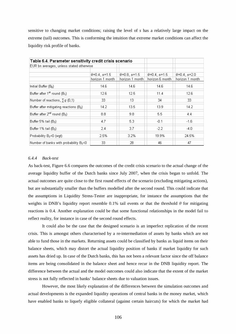
106

sensitive to changing market conditions; raising the level of s has a relatively large impact on the

extreme (tail) outcomes. This is conforming the intuition that extreme market conditions can affect the

liquidity risk profile of banks.

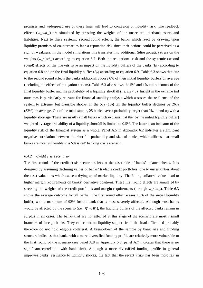
6.4.4 Back-test

As back-test, Figure 6.6 compares the outcomes of the credit crisis scenario to the actual change of the

average liquidity buffer of the Dutch banks since July 2007, when the crisis began to unfold. The

actual outcomes are quite close to the first round effects of the scenario (excluding mitigating actions),

but are substantially smaller than the buffers modelled after the second round. This could indicate that

the assumptions in Liquidity Stress-Tester are inappropriate, for instance the assumptions that the

weights in DNB’s liquidity report resemble 0.1% tail events or that the threshold θ for mitigating

reactions is 0.4. Another explanation could be that some functional relationships in the model fail to

reflect reality, for instance in case of the second round effects.

It could also be the case that the designed scenario is an imperfect replication of the recent

crisis. This is amongst others characterised by a re-intermediation of assets by banks which are not

able to fund those in the markets. Returning assets could be classified by banks as liquid items on their

balance sheets, which may distort the actual liquidity position of banks if market liquidity for such

assets has dried up. In case of the Dutch banks, this has not been a relevant factor since the off balance

items are being consolidated in the balance sheet and hence recur in the DNB liquidity report. The

difference between the actual and the model outcomes could also indicate that the extent of the market

stress is not fully reflected in banks’ balance sheets due to valuation issues.

However, the most likely explanation of the differences between the simulation outcomes and

actual developments is the expanded liquidity operations of central banks in the money market, which

have enabled banks to liquefy eligible collateral (against certain haircuts) for which the market had

107

seized up. By doing so, central banks addressed a market failure, by breaking the loop between market

and funding liquidity risk and preventing further market distress (Nikolaou, 2009). In terms of our

model, this implies that the value of certain collateral does not fully reflect the second round effects of

the market turmoil (which have come to the fore in reduced liquidity and fallen mark-to-market

values, in particular for structured credit securities which, in some cases, is eligible collateral for

central bank borrowing). The simulation outcomes on the other hand, are dominated by the adverse

second round effects on the liquidity buffers (in the scenario, the central bank facilities are only

included implicitly and partially, i.e. for the banks which react through pledging collateral at the

central bank).

In the next chapter, the Liquidity Stress-Tester model is extended with a reaction function of

the central bank. With that extended model, the mitigating effects of additional liquidity supply and

asset purchases by the central bank on the second round effects of a scenario are simulated.

-70%

-60%

-50%

-40%

-30%

-20%

-10%

0%

1month 6 months

Actual outcome Scenario, 1st round Scenario, 2nd round

Figure 6.6. Back-testing the scenario outcomesChange of liquidity buffer since July 2007 (monthly data, average Dutch banks). Model parameters: θ=0.4; s =1.5

6.5 Conclusions

Liquidity Stress-Tester is an instrument to simulate the impact on banks of shocks to market and

funding liquidity. It takes into account the important drivers of liquidity stress, i.e. on and off balance

sheet contingencies, feedback effects induced by collective reactions of heterogeneous banks and

idiosyncratic reputation effects. Contagion results from the effects of banks’ reactions on prices and

volumes in the markets where the banks are exposed to. The model contributes to understand the

influence on liquidity risk of collective reactions by banks, the level of market stress and the length of

the scenario horizon. These factors have been main drivers of the recent financial crisis. Liquidity

Stress-Tester could be used by central banks to stress-test the liquidity risk at the level of the financial

108

system. In this chapter the model has been applied to Dutch banks, but it could also be applied to other

countries’ banking systems, provided that data for liquid assets and liabilities are available on an

individual bank level. The parameters of the model (such as the weights and the threshold for

reactions) can be tailored to a local banking sector, according to the insights of the supervisor or

central bank.

The model outcomes lend support to policy initiatives to enhance the liquidity buffers and

liquidity risk management at banks, as recently proposed by the Basel Committee and the FSF (FSF,

2008). A sufficient level of liquidity buffers limits idiosyncratic risks to a bank, by providing

counterbalancing funding capacity to weather a liquidity crisis. Moreover, buffers are important to

reduce the risk of collective reactions by banks and thereby to prevent the risk of amplifying effects

and instability of the financial system as a whole. Admittedly, this should be considered in conjunction

with the cost of holding higher liquidity buffers, also on the macro level of the financial system. To

assess such equilibrium effects one would perhaps need a more stylised model of the financial system.

Holding liquidity buffers should be part of sound liquidity risk management, which identifies

and measures the full range of liquidity risks, including the interaction between market and funding

liquidity and potential feedbacks on banks’ reputation related to signalling effects or flawed external

communication. Furthermore, to fully grasp the liquidity risk of a bank, stress-tests should cover the

group-wide liquidity exposures on a consolidated basis, including the risks of multi-currency

exposures, complex instruments and off balance sheet contingencies. These factors are included in

DNB’s liquidity report which has proven to be useful for Dutch banks and the supervisor, particularly

during the recent market turmoil. Based on the features of the liquidity report, Liquidity Stress-Tester

provides a tool to evaluate the importance of the various risk factors for banks’ liquidity positions in

different scenarios.

109

Appendix 6.1 Stylised balance sheet bank Y (base line)

110

Appendix 6.2 Impact banking crisis scenario

-40%

-30%

-20%

-10%

0%

0% 5% 10% 15% 20% 25% 30% 35%

Panel A.1 Bank size and 1st round impactImpact (E1 / Bo), share in total sectors' assets (x-axis)

Corr 0.06

-40%

-30%

-20%

-10%

0%

0 20 40 60 80

Panel A.2 Funding diversification and 1st round impactImpact (E1 / Bo), kurtosis of funding structure (x-axis)

Corr -0.05

High diversification Low diversification

0

1

0% 5% 10% 15% 20% 25% 30% 35%

Panel A.3 Bank size and reactionTrigger for reaction (0,1), share in total sectors' assets (x-axis)

Corr -0.15*

* significant at 10% confidence

0

1

0 20 40 60 80

Panel A.4 Funding diversification and reactionTrigger for reaction (0,1), kurtosis of funding structure (x-axis)

Corr -0.13*

High diversification

Low diversification

* significant at 10% confidence level

0%

25%

50%

75%

100%

0% 5% 10% 15% 20% 25% 30% 35%

Panel A.5 Bank size and shortfall probabilityProbability B3<0, share in total sectors' assets (x-axis)

Corr -0.11*

* significant at 10% confidence

0%

25%

50%

75%

100%

0 20 40 60 80

Panel A.6 Funding diversification and shortfall probabilityProbability B3<0, kurtosis of funding structure (x-axis)

Corr -0.06

High diversification

Low diversification

Notes 1) The banking crisis scenario assumes a withdrawal of non-bank deposits and other funding by professional money market players, other institutional investors and corporates and by withdrawals of savings deposits by households. 2) Panels A.1, A.3 and A.5 show the relationship between bank size on the horizontal axis and the impact of the first scenario round (A.1), the probability of reaction (A.3) and the probability of B3 < 0 (A.5) on the vertical axis. In panels A.2, A.4 and A.6, the diversification of funding is on the horizontal axis (as approximated by the kurtosis of the liability structure of banks’ balance sheets).

111

Appendix 6.3 Impact credit crisis scenario

-40%

-30%

-20%

-10%

0%

0% 5% 10% 15% 20% 25% 30% 35%

Panel A.7 Bank size and 1st round impactImpact (E1 / Bo), share in total sectors' assets (x-axis)

Corr -0.1

-40%

-30%

-20%

-10%

0%

0 10 20 30 40 50 60 70 80

Panel A.8 Funding diversification and 1st round impactImpact (E1 / Bo), kurtosis of funding structure (x-axis)

Corr +0.31**

High diversification Low diversification

** significant at 5% confidence level

0

1

0% 5% 10% 15% 20% 25% 30% 35%

Panel A.9 Bank size and reactionTrigger for reaction (0,1), share in total sectors' assets (x-axis)

Corr +0.24**

** significant at 5% confidence level

0

1

0 10 20 30 40 50 60 70 80

Panel A.10 Funding diversification and reactionTrigger for reaction (0,1), kurtosis of funding structure (x-axis)

Corr -0.27**

High diversification

Low diversification

** significant at 5% confidence level

0%

25%

50%

75%

100%

0% 5% 10% 15% 20% 25% 30% 35%

Panel A.11 Bank size and shortfall probabilityProbability B3<0, share in total sectors' assets (x-axis)

Corr -0.05

0%

25%

50%

75%

100%

0 10 20 30 40 50 60 70 80

Panel A.12 Funding diversification and shortfall probabilityProbability B3<0, kurtosis of funding structure (x-axis)

Corr -0.10

High diversification

Low diversification

Notes 1) The credit crisis scenario assumes declining values of banks’ tradable credit portfolios, due to uncertainties about the asset valuations which cause a drying up of market liquidity. The falling collateral values lead to higher margin requirements on banks’ derivative positions. 2) Panels A.7, A.9 and A.11 show the relationship between bank size on the horizontal axis and the impact of the first scenario round (A.7), the probability of reaction (A.9) and the probability of B3 < 0 (A.11) on the vertical axis. In panels A.8, A.10 and A.12, the diversification of funding is on the horizontal axis (as approximated by the kurtosis of the liability structure of banks’ balance sheets).

112