university of havvai'1 library investment …...business arrangement corresponds to an...
TRANSCRIPT
UNIVERSITY OF HAVvAI'1 LIBRARY
INVESTMENT UNDER UNCERTAINTY:
APPLICATION OF BINOMIAL OPTION ANALYSIS
TO DEVELOPMENT OF GEOTHERMAL ENERGY IN INDONESIA
A DISSERTATION SUBMITTED TO THE GRADUATE DIVISION OF THEUNIVERSITY OF HAWAI'I IN PARTIAL FULFILLMENT OF THE
REQUIREMENTS FOR THE DEGREE OF
DOCTOR OF PHILOSOPHY
IN
ECONOMICS
DECEMBER 2002
ByAsclepias Rachmi Soerjono Indriyanto
Dissertation Committee:
U.ijayant Chakravorty, ChairpersonSumner La CroixAndrew Mason
Fereidun FesharakiNicholas Ordway

© Copyright 2002
by
Asclepias Rachmi Soerjono Indriyanto
iii

To my parents:
Soerjono Soedibjo - in memoriam
and
Jussilvia M. Roosrnailie
iv

ACKNOWLEDGEMENTS
A great many people have knowingly and unknowingly contributed to this
accomplishment. Their care, love and patience have given me strength and have helped
me overcome many difficulties along the way. Since I might not be able to express my
gratitude adequately, I pray to Allah for His blessings over every one of them.
I would like to thank Professor Chakravorty for his advice and willingness to
chair the committee, Professor Mason for his thoughtful comments, and Professor
Ordway for his ideas and radiant energy that has been contagious. I would especially like
to express my appreciation to Professor La Croix for his helpful guidance and constant
encouragement, and to Dr. Fesharaki for his tremendous support in many forms that
made things possible.
I am indebted to my dear friends Widyanti Soetjipto, Widhyawan Prawiraatmadja,
and Wiwik Bunjamin, who are my life support during the hard times away from home. I
also thank Gayle Sueda for her generous assistance to ensure a pleasant work
environment and to endure the pain in editing the manuscript.
Fina1ly, I would like to express my sincere gratitude to my husband Hartono
Indriyanto, our children Dita and Baska, and our extended family, which have been very
patient and compassionate during this long journey.
v
ABSTRACT
Indonesia has identified a large amount of geothermal resource potential
throughout the islands. However, geothermal utilization is presently low. One of the
main reasons is due to limited government funds to develop the resources. Another
contributing factor is the high prices charged by private geothermal electricity producers,
which was part of the reason why the government suspended most private geothermal
development projects. The common perception blames corruption, collusion and
nepotistic behavior of the market participants for this unfortunate situation.
This research shows that even if opportunistic behavior is cast away, the present
business arrangement corresponds to an incentive system that brings about high
geothermal electricity prices. Applying the Real Option Theory reveals that managerial
flexibility in the decision-making process of a geothermal project is valuable, since it
allows the use of updated information.
In contrast to the present ex-ante price detennination setting, a possible way to
incorporate flexibility is to agree on output price after exploration activities are
concluded. Under certain conditions, this ex-post price determination setting may
produce a wider range of feasible prices that includes those lower than the ex-ante price.
As such, incorporating flexibility into the decision process improves project value and
may lower its output price.
The research model implicitly assumes the first-best world with respect to the
assumptions of symmetric information and a simple self-interest behavior. These two
assumptions set the limitation of the model results. In a complex world with incomplete
vi

and asymmetric information as well as opportunistic behavior of the market participants,
the ex-post price determination is likely to fail due to reciprocal concerns of the parties.
A two-phased negotiation system may attenuate the opportunism concerns, while
provides assurance that only viable projects can survive.
vii

TABLE OF CONTENTS
Acknowledgements v
Abstract vi
List of Tables xi
List of Figures xii
Chapter 1:
1.1
1.2
1.3
1.4
Chapter 2:
2.1
2.2
2.3
2.4
Introduction ..
The Electricity Sector .
Research Boundaries .
Uncertainty Issue .
Chapters Outline .
1.4.1 Investment Literature and Practices .
1.4.2 Research Contribution .
1.4.3 Geothermal Development in Indonesia .
1.4.4 Real Option Analysis for a Geothermal Project .
1.4.5 Policy Implications .
Investment Opportunity .
Investment .
2.1.1 Theory versus Observed Investment Behavior .
2.1.2 Investment Under Uncertainty .
2.1.3 Investment as Option: Implementation .
Financial Options .
2.2.1 Basic Features .
2.2.2 Valuations .
2.2.3 Black-Scholes Formulation .
2.2.4 Binomial Lattices Framework .
Real Options .
2.3.1 Characteristics of Real Options .
2.3.2 Real Option Representations .
Investments Valuations .
2.4.1 Capital Budgeting .
2.4.2 Options-Based Models .
2.4.3 Graphical Models .
viii
1
2
5
8
10
10
14
14
16
18
21
22
23
25
31
33
34
36
40
44
50
51
54
60
63
65
68

2.5
Chapter 3:
3.1
3.2
3.3
3.4
Chapter 4:
4.1
4.2
Chapter 5:
5.1
5.2
5.3
5.4
Chapter 6:
6.1
2.4.4 Finding Solutions .
Research Methodology ..
Research Objectives ..
Modeling .
Impact of Flexibility in Project Assessment ..
Alternative Business Arrangement ..
Literature Contribution ..
Geothermal Development in Indonesia .
Geothermal Resources ..
4.1.1 Geothermal Extraction ..
4.1.2 Geothermal Utilization ..
Geothermal in Indonesia .
4.2.1 Resource Potential .
4.2.2 Resource Utilization .
4.2.3 Business Environment ..
4.2.4 Perspective for Modeling ..
The Value of Investment Opportunity .
Net Present Value Assessment .. , ..
5.1.1 Model Structure ..
5.1.2 Information and Data for the Base Case Model ..
5.1.3 Decision Tree Assessment .
5.1.4 NPV ofthe Upside Potential ..
Real Option Perspective .
5.2.1 Step 1: Compute the Base Case PV of the Project .
5.2.2 Step 2: Model the Uncertainty of Project Value
using Event Tree ..
5.2.3 Step 3: Identify and Incorporate Managerial Flexibility ..
5.2.4 Step 4: Analysis ..
Expansion Option .
5.3.1 Exploration Information .
5.3.2 Expansion Simulation .
Exercise Summary .
Policy Implication ..
Interrelationship of the Parties .IX
70
75
7980
80
81
81
83
84
85
87
88
88
90
92
100
102
105
106
108
119
122
129
131
131
134
142
145
146
149
ISS159
160

REFERENCES .
6.2
6.3
6.4
Appendix A:
Al
A2
A3
AppendixB:
Appendix C:
C.l
C.2
C.3
C.4
C.5
C.6
C.7
C.8
AppendixD:
D.l
D.2
D.3
D.4
Ex-Post Price Determination ..
Two-Phase Negotiation .
Concluding Remarks .
Models for Investment Valuation: Strength and Weaknesses ..•
Option-Based Models ..
Decision Trees .
Influence Diagrams .
Geothermal Development in Indonesia .
Influence Diagrams .
The Family of Decision Analysis ..
Influence Diagrams Framework ..
A Formal Representation .
Graph Elements and Structure .
Evaluation Procedure .
Commercial Software for Implementation .
The Base Case Model ..
Model with Two-Phase Negotiation ..
Simulation Input-Output .
Inputs for Geothermal Electricity Model (GEM); Base Case .
Simulation Results of GEM .
Real Option Valuation for a Smaller Variation in Field Data ..
Real Option Valuation for a Larger Variation in Field Data .
164
166
168
170
170
171
173
174
182
182
185
188
192
195
199
201
207
210
211
216
223
225
227
x

1-1.
1-2.
2-1.
2-2.
2-3.
2-4.
2-5.
4-1.
4-2.
5-1.
5-2.
5-3.
5-4.
5-5.
5-6.
5-7.
5-8.
5-9.
5-10.
5-11.
5-12.
5-13.
5-14.
LIST OF TABLES
Share of Energy Utilization (%) ..
Detenninants of Option Value .
Real Options Application .
Methods to Value and Model Investment Opportunity ..
Option-Based Models .
Which Approach is Appropriate? .
General Approach to Apply Real Option to the Real World Problem ..
Classification of Geothermal Resources ..
Geothermal Resource Potential in Indonesia .
Notes for the Arcs .
Unit Cost of Power .
Chance Nodes ..
Decision Nodes ..
Deterministic Nodes .
Major Results of Upstate NPV Assessment .
Parameter Values for Monte Carlo Simulation z .
A Wider Range of Parameter Values .
Reserve Estimates Before and After Exploration ..
Simulation on Plant Size and Output Price ..
Potential Savings from Flexible Arrangement in Geothermal Project .
Geothermal Power Plant Development Project .
Production Cost (US$ centslkWh) ..
Results Summary .
Xl
6
12
32
62
66
71
7586
90
109
113
120
120
121
128
134
143
148
149
152
154
155
157

2-1.
2-2.
2-3.
4-1.
4-2.
5-1.
5-2.
5-3.
5-4.
5-5.
5-6.
5-7.
5-8.
5-9.
5-10.
5-11.
5-12.
5-13.
5-14.
6-1.
LIST OF FIGURES
Lattices of the Three Assets
Option Value of a Two-Period Lattice .
Relations of Research Model and the Literature .
Location of Some Large Geothermal Prospects an Existing Facilities ..
Progress in a Geothermal Project .
Research Outline ..
Uncertainties and Major Decisions in the Base Case Model .
Electricity Consumption .
Indonesia Discount Rates .
Project Decision Structure in Tree Representation ..
Expected Value Assessment for Project Without Flexibility ..
Base Case Sensitivity Analysis ..
Some Project Indicators .
Event Tree for Project Value .
Sequential Compound Options ..
Value Tree of the Second Option ..
Decision Tree for the First Option .
Impact of Parameter Value Range to Probability Distribution of z .
Geothermal Price and Average Production Costs of the Load System .
Project with Two-Phase Negotiation ..
xu
45
48
76
89
93
104
106
111
116
123
124
125
126
134
138
139
140
144
153
167

CHAPTER 1
INTRODUCTION
Indonesia has identified a large amount of geothermal resource potential
throughout the islands. However, geothermal utilization is presently low. One of the
main reasons is due to limited government funds to develop the resources. Another
contributing factor is the high prices charged by private geothermal electricity producers,
which was part of the reason for the establishment of the government policy to suspend
most private geothermal development projects. The common perception blames
corruption, collusion and nepotistic behavior of the market participants for this
unfortunate situation.
This research shows that even if opportunistic behavior is cast away, the present
business arrangement corresponds to an incentive system that brings about high
geothermal electricity prices. Applying the Real Option Theory reveals that managerial
flexibility in the decision-making process of a geothermal project is valuable, since it
allows the use of updated information. In contrast to the present ex-ante price
detennination setting, a possible way to incorporate flexibility is to agree on output price
after exploration activities are concluded. Under certain conditions, this setting may
produce a wider range of feasible prices that includes those lower than the ex-ante price.
As such, incorporating flexibility into the decision process improves project value and
may lower its output price.
The research model implicitly assumes the first-best world with respect to the
following two assumptions: (i) symmetric information, which means market participants
1

reveal full information when requested, and (ii) minimal opportunistic behavior, which
means while maximizing profits; parties are trustworthy and lawful. These two
assumptions set the limitation of the model. In a complex world with incomplete and
asymmetric information as well as opportunistic behavior, there are implications from
incorporating flexibility into the decision process. Although a full study regarding this
issue is beyond the scope of this research, an informal discussion in the last chapter
addresses some concerns.
This chapter provides a background for the research framework. The first section
illustrates the complexities of problems in the electricity sector in Indonesia. The second
section specifies the research boundaries. The third section discusses the reasoning of
considering uncertainty as an important issue in the research model. The fourth section
summarizes the other chapters in this dissertation.
1.1 THE ELECTRICITY SECTOR
Electricity development in Indonesia had remarkable statistics indicated by,
among others, a higher than 10% per year average growth in installed generating capacity
as well as consumption during the 1980s and early 1990s. However, the electricity sector
has been in turmoil following the Asian financial crisis that also hit the country in mid
1997. In only four months the Rupiah, the Indonesian currency, lost 80% of its value.
This severe depreciation also posed significant impacts on PLN, the state-owned utility
company, which carried heavy US$ debts for infrastructure investments. Moreover, PLN
had obligations to pay billions of US$ to independent power producers (IPP) under
several existing long-term power purchase agreements (PPAs).
2

In late 1997, the government was forced to seek a bailout package organized by
the International Monetary Fund (IMF). Motoyarna and Widagdo (1999) cite a PLN
audit report dated 1999, conducted by Arthur Andersen under the instruction ofthe IMF:
'The audit report reveals that PLN has to bear a total loss of ... approximatelyUS$29.8 billion, which is about one and a half times the State Budget ofIndonesia. Andersen likewise reports that of these incurred losses, US$18 billionis attributable to the abuse of power in the private power purchase agreements ... ,US$1O.7 billion as losses caused by the increased exchange rate, and US$1.5billion from the inefficiency of PLN operation."
PLN was on the brink of bankruptcy that it needed to operate under massive
government subsidies. It was unable to fulfill its obligation to purchase electricity under
its PPAs. Shortly afterwards, this was fol1owed by the suspension of 27 IPP projects with
a combined capacity of about 15,000 MW by Presidential Decree No. 37/1997. Although
a later revision of the policy reduced the suspension to 16 IPP projects, such disruption
has yielded several arbitration and litigation cases (Seymour and Sari, 2002; World
Energy Council, 2001; Motoyarna and Widagdo, 1999).
The participation of IPPs in the Indonesian electricity sector has been
controversial. On the one hand, the World Bank as a major donor in late 1980s suggested
that PLN should pursue a strategy of deregulation, decentralization and competition in
order to move from bureaucracy to enterprise. Further, they suggested the government,
albeit with caution, consider attracting private capital to finance the rapidly increasing
demand for electricity as wel1 as to compete with PLN. Competition forces power
generators to innovate and operate in the most efficient and economic manner in order to
remain in the business and recover their costs, thereby benefiting consumers
(Bhattacharya et al., 2001). Hence, private participation was initiated to become one of
3

the drivers for a continuous strong growth of the sector and to provide better service to
the customers.
On the other hand, the implementation of this strategy led to several concerns: (i)
indication of corruption, since most negotiations took place in unsolicited, non-
transparent bidding processes, resulting in higher than estimated costs, high prices,
dollar-pegged, and take-or-pay conditions that were commonly considered as in favor of
project investors, (ii) large excess generating capacity that showed unwarranted
investment, and (iii) involved indirect pressures from donor governments (Seymour and
Sari, 2002; Smith, 2002; Institute for Policy Studies and The Transnational Institute,
2001; Howard, 1999).
Among the three concerns, corruption is recognized as one of the biggest
problems in Indonesia. There have been a lot of discussions and movements to eradicate
corruption.' However, its severity remains (Asian Development Bank, 2002; Perlez,
2002).
By now, the Asian crisis has caused multi-dimensional problems in all sectors of
the Indonesian economy. The Rupiah stays at around 300% lower value than it was in
early 1997. This means that PLN debts to lenders as well as having to fulfill its existing
obligations to the IPPs has worsened into three times larger in terms of the local currency.
As PLN eams its revenue from electricity consumers, this financial burden eventually
falls on the public in the form of significantly higher prices of electricity. In addition, the
pattern of an ever-increasing government budget for subsidy allocation is not sustainable.
1 For example, documents produced by Partnership for Governance Reform in Indonesia (2002), Harahap(1999), and Motoyama and Widagdo (1999) show collaboration among many groups both inside andoutside Indonesia, including some international donor agencies, that share similar concerns.
4

This means there are pressures for gradual elimination of various forms of energy
subsidies, which translates into an increasing trend of prices. Combining these factors, it
is clear that price adjustments are inevitable. Nevertheless, it has never been an easy task
to raise prices when the economy is in distress. The social, political, and security
concerns have been complicating the adjustment process.
In summary, most of the public concerns have been focused on the governance
issues and opportunism behavior of the market participants. It is also widely recognized
that the implementation of the strategies drafted to improve these aspects would take
significant time. The ongoing price adjustments are inevitable, but the implementations
have been a delicate matter. The whole picture above illustrates the problems and the
dynamics of efforts to improve the electricity sector in Indonesia.
1.2 RESEARCH BOUNDARIES
Against this backdrop, the initial interest toward geothermal electricity
development was mainly motivated by the following two ironies:
(i) Geothermal resource potential is estimated to be around 20,000 MWe,2 which is
comparable to the current size of PLN generating capacity of combined energy
sources. Despite this large estimated potential, there is only 787 MW installed
capacity at the moment.
(ii) In contrast to the merit dispatch order, some private geothermal projects with high
electricity prices are determined as base load suppliers.
2 Stands for MegaWatt energy, which reflects equivalent energy to generate electricity of that amount.
5

The first issue is important with respect to the government policy to diversify the
domestic energy utilization. Table 1-1 shows that this policy works for fossil fuels, but
has a very small effect on geothermal and none on renewable energy resources (Ariati,
2001). It can be argued that there has been no significant progress towards sustainability
in the energy sector, although this may be due to the instability of the currency
(Soejachmoen, 2002). Furthermore, combinations of high growth in electricity demand
even during the crisis years, decreasing oil production, and tight government budget
allocation for imported fuels, calls for more utilization of endogenous energy. A large
potential of geothermal energy, which can only be used in the surrounding area, is a good
candidate for meeting domestic need.
The second issue is important since as discussed earlier, high prices that are also
linked to US dollar had imposed a heavy financial burden to the utility company and led
to a halt in geothermal development projects in recent years.
Table 1-1. Share of Energy Utilization (%)
1970 1998
00 88 59------_.•.__._--------_.- -------_."."--,".-_.•.•...,.•.•.•._-,_.- -"._".---_.•._-----_.•._----_.•.•.•.•.•Gas 6 25••........_....._....•..- •..............._._- •.••••••...•.....•............•........•...•-Coal 1 191--:.•.._-_•......................•.....•••.._ ......•......_ .._ _ ....•._Geothermal 0 1·H~dfo··--············· ······-5--··········· ·_······-5-·_·Source: Ariati (200I)
The research aims to look at possibilities to improve the utilization of geothermal
energy in Indonesia. Nevertheless, considering the peculiarities in the geothermal
electricity sector and the larger problems in the Indonesian economy in the background, it
6

was not immediately clear as to how and where to find the possible answers. Are these
all about opportunism behavior? Would moral or ethical issues, problems in the legal and
judicial system, an unfinished agenda in civil service reform, and inadequate public
sector spending describe the driving forces behind the problem? Chances are that all of
these factors are intertwined, but also that it would be difficult to distinguish their effects
individually. A candidate framework for understanding the complexity and diversity of
overall institutional arrangements across the economy would be the Comparative
Institutional Analysis approach introduced by Aoki (2001).
On the contrary, this research focuses on the geothermal project itself and less
emphasis on the other problems in the electricity sector and the Indonesian economy to
avoid the above overwhelming complexities as the starting point. Further, the research
concentrates on the significance of natural characteristics of geothermal resources to the
project. The benefit of restricting the interest span is to help isolate some inherent issues
specific to geothermal electricity projects. On the other hand, a drawback of this
approach is that the model does not facilitate a direct examination on strategic behavior
of the parties involved in this activity. However, insights on the distinctive nature of
geothermal resource developments may compensate this disadvantage and may serve as a
base for more complex settings. Based on the research findings, Chapter 6 extends the
analysis to address this concern. Another drawback is an unclear picture of the findings
impact on the utilization of geothermal energy resources of the country, since the latter
also depends on various other factors beyond the project boundary such as investment
climate of the economy. Nevertheless, the research findings point toward specific ways
7
that can be used to facilitate the transaction process between the government and
potential private developers.
1.3 UNCERTAINTY ISSUE
Investment requires pre-commitment of resources in order to obtain later benefits.
As many sources of uncertainty may affect actual benefits to be received, the initial
decision to devote the resources mayor may not be worthwhile. The intricacy of many
factors that come into play makes investment decisions under study for a long time.
In a geothermal electricity project, the future benefits would come from sales of
converting geothermal energy into electricity, and these future benefits should be large
enough to cover the previous expenditures and some profits. The project involves large
capital outlays during early years, which are mostly used to obtain more information and
knowledge about economic feasibility of the prospect area. Table B-2 in Appendix B
illustrate the magnitude of average capital requirement in the existing geothermal projects
in Indonesia. Major allocation of capital during this exploratory stage of the project is to
drill some wells, which would reveal underground characteristics of the reserve that
provide inputs to estimations of reserve size and additional capital requirements. When
such search concludes the presence of a feasible reserve, further expenditures are
required to prepare for production activities. These costs are mostly for drilling more
wells and constructing necessary systems to develop the field as well as power plant
8

facilities. Earnings would start only after exploration and development stages are
completed.3
A project with the above characteristics is considered risky due to (i) uncertainty
in resource existence, quality, and feasibility; (ii) the sizeable capital to be invested early
on; and (iii) the lead time of studies and preparation before the project generate earnings.
As the resource base is uncertain to begin with, the future earnings of the project are also
uncertain. These features show that uncertainty is a major factor in this case.
Furthermore, the institutional economics literature, such as works on transaction
costs and incentives treat uncertainty as a precondition for the settings or a prior base of
knowledge:
"But for uncertainty, problems of economic organization are relatively uninteresting. Assume, therefore, that uncertainty is present in non trivial degree ..."(Williamson, 1985)
"The problem of managing information flows was the fIrst research topic foreconomists, once they mastered behavior under uncertainty ... " (Laffont andMartimort, 2002)
Since uncertainty is a necessary condition, the subject deserves a closer attention. This
translates to examining the implications of recognizing the fact that uncertainty is
signifIcant in the geothermal electricity case. The issues of opportunism and incentives
may enter the discussion, but the main approach for this research is based on uncertainty
consideration. Therefore, a growing literature on 'investment under uncertainty' is
consulted to fInd a suitable methodology.
J Partial development, such as completing I x 55 MW facility of the total 2 x 55 MW planned capacity, ispossible.
9

1.4 CHAPTERS OUTLINE
The following subsections serve as a brief summary of the rest of the chapters in
this dissertation. The first part represents Chapter 2 that discusses the literature on
investment and uncertainty. The second part corresponds to Chapter 3 about research
contribution. The third part sketches the issues on geothermal development in Indonesia,
which details are presented in Chapter 4. The fourth part abridges Chapter 5,
highlighting some notes on the application of real option analysis to an investment
opportunity in geothermal electricity project. The last part underlines some policy
implications discussed in Chapter 6.
1.4.1 Investment Literature and Practices
The rules of optimal investment behavior and major determinants of investment
decisions in economic theory are not consistently observed in the actual business
practices. The literature on investment under uncertainty is one of the theoretical
explanations that attempt to reconcile the gap between investment theory and the
observed corporate investment behavior.
The way investments are modeled and assessments are conducted may affect the
value attached to the project and its components, as well as the expected future benefits
from investment activities. Inappropriately ignoring some of the project features may lead
to under-valuation and consequently overlook potentially good investment candidates.
There are two major groups of work in the investment under uncertainty
literature, which are (i) The Orthodox Theory, and (ii) The Options Approach. The first
group consists of works based on individual or combinations of the following theories: q
10

theory of investment, as well as frictions in investment decision such as adjustment cost
and irreversibility. The underlying principle of investment decision in these works is the
net present value (NPV) rule, which is to select a project with positive NPV and to reject
otherwise. The NPV rule has been widely used, although implementations mayor may
not comply with the underlying assumptions of the theory. Nevertheless, this practice
does not allow later decisions to be incorporated into the initial investment valuation.
The second group of approach perceives investment opportunity as an option.
Spending initial investment to acquire an investment opportunity does not necessarily
require the investor to invest again in the future. Instead, holding investment
opportunities allow investors to have a portfolio of future decisions. This translates to
flexibility in management decisions, which can be exercised to improve profits or to
mitigate losses.
The theory of measuring how much an option is worth originates in the financial
options literature. A financial option is a contract that provides the holder a right but not
an obligation to buy or sell the underlying financial asset at a predetermined price at a
certain future date. Widely known methods to value financial options are (i) those based
on the Black-Scholes (1973) formulation, and (ii) based on the Binomial Lattice
framework introduced by Cox-Ros-Rubinstein (1979). Both methods are based on the
no-arbitrage principle, i.e., they value options by combining two available securities with
known payoff to construct a portfolio that reproduces the local behavior of the derivative
security (Luenberger, 1998). The basic difference between the Cox et al. method and the
Black-Scholes formulation is the assumption of how asset price fluctuates. B1ack
Scholes assume that the price of the underlying asset fluctuates following an Ito process,
11

which means the approach employs continuous representation of stochastic behavior of
the price. Cox et al. assumes binomial distribution with symmetrical up and down steps,
which represents fluctuation of the price of the underlying in discrete time.
Table 1-2 lists six variables that determine the value of options. The original
Black-Scholes formulation involves only five variables, since it assumes there are no
dividends payments during the life of the option. Merton (1973) generalizes the
formulation to include dividend payments. These same sets of variables also determine
the value of non-financial or real options. The first column of Table 1-2 lists these
variables in real option context. In addition, the value of real options may be affected by
other variables that characterize the complex setting of the problem.
Table 1-2. Determinants of Option Value
The effect of an increaseDeterminants in the value of a
_._--_._.-_.-._._..._-----_._.__._-_._--...__ ._._._._.-""" --_._--_...-. __.._._._...• determinant____...__..._____........... "-----_-_-_"0-.0.0.0..___..._----
Real Option Financial Option Call Put
Value of the underlying asset Stock Price Increase Decrease
Exercise price or investment cost Strike Price Decrease Increase
Standard deviation of the value of Volatility of Stock Increase Increasethe underlying asset Price
Time to expiration of the option Time to expiration of Increase Increasethe option
Risk-free rate of interest Interest Rate Increase Decrease
Dividends payout Cash Dividends Decrease Increase
Source: Copeland and Antikarov (2001), Bodle and Merton (2000)
12

Although the real option concept is compelling and has been explored in the
literature for more than a decade, its implementation is still considered at infancy. The
reasons for the slow development are: (i) the complexities surrounding real options, (ii)
some significant uncertainties will likely remain at the time of real option decision, and
(iii) highly sophisticated mathematical techniques in the literature.
Copeland and Antikarov (2001) proposes an approach that can overcome some
parts of the first and third obstacles above, namely identifying the underlying asset,
estimating its value, as well as the technique of assessing the real option value. There are
two necessary assumptions for this approach. The first assumption is called the Marketed
Asset Disclaimer, which uses the present value of the project itself as the underlying
risky asset in place of the 'twin security' in the financial option theory. The second
assumption asserts that properly anticipated prices fluctuate randomly; therefore, the rate
of return on any security would be a random walk. Samuelson (1965) proves the latter
assumption, and Copeland et al. (2001) conduct an empirical study to show that, based on
Samuelson's proof, it is also true that real equity returns on properly anticipated streams
of cash flow fluctuate randomly.
Another work that is used as a reference in this research is Cortazar et al. (2001),
which evaluates a natural resource extraction project. The extraction-development
production stages of the project are modeled as sequential compound options. All phases
are optimized contingent on price and geological-technical uncertainty. The model
collapses price and geological-technical uncertainties into a one-factor model.
13

1.4.2 Research Contributions
Despite keen interests of various parties to develop geothennal resources in
Indonesia, the existing fundamental problems have led to very little or no progress in
recent years. Motivated by the present unfortunate condition of geothermal development,
this research aims to:
1. Model a geothermal development project using options theory. This approach is
expected to enable a wider perspective and better understanding of the present
problems in geothermal development in Indonesia.
2. Compare options-based to the standard NPV decision-making.
3. Explore alternative arrangements that are potentially Pareto improving to induce
geothermal development.
4. Contribute to the literature on real option and natural resource development in the
following ways:
• The application to geothermal development adds to the body of works in real
option analysis on natural resource extraction. In addition, this case combines
natural resource extraction with electricity generation activities, which are usually
treated as separate subjects.
• The case highlights the problem of non-traded underlying asset and the way to
overcome this barrier to enable the application of real option approach.
1.4.3 Geothermal Developments in Indonesia
Indonesia has identified 244 geothennal prospect areas all over the islands, with
estimated potential capacity of around 20,000 MWe. Appendix B shows the locations of
14

these identified geothennal potentials. However, after 20 years of development, there are
only 787 MW installed geothermal plant capacity and among them merely 525 MW in
operation.
Significant factors causing the slow progress are the existing business
arrangements where output price is set before the project starts and the limited initial
infonnation about the prospect areas due to restricted government funding. In addition,
some geothermal projects operate under Build-Operate-Transfer contract, where private
operators are required to transfer plant ownership to the utility company around the
midlife of the project operation. This means investors need to recover a portion of their
capital outlay in a shorter period of time. These factors combined cause high prices of
geothermal electricity supplied by private operators.
A geothermal project is characterized by large capital outlay during the early
years, sometimes much higher than that of a similar plant using conventional fuel.
However, in a geothermal plant, the energy component costs far less than those of
conventional fuels. Therefore, the savings in energy costs should recover the higher
capital outlay. Since savings in energy costs are obtained over time, geothermal plants
should be designed to have a long enough lifetime to amortize the initial investment
(Dickson et al., 1995). In addition, this investment profile suggests that a viable
geothermal power requires consistently high revenue, which means steady sales. This
condition implies that it effectively competes only with base load power sources (Blair et
aI., 1982).
The existing geothermal power plants in Indonesia are treated as a 'must-run,'
which means they are supplying the base load of the system. This policy is a
15

consequence of contractual obligations that requires the utility company to purchase the
power produced by these plants. However, the high prices of some geothermal plants
actually position them at a lower order in the merit system of a dispatch. Without the
'must-run' policy and if other base load suppliers can provide the amount at a lower
price, the utility company would be better off without supplies from these expensive
geothermal plants. A pure merit system of load dispatch would leave these plants out of
the system. Hence, geothermal plants are not competitive.
The economic crisis that started in 1997 had strong effects on geothermal
development. The government suspended 16 private power generation projects that
included seven geothermal projects. These suspensions were followed by legal disputes
between several developers on one side and the electric utility company, Pertamina and
the government of Indonesia (GOI) on the other side. Despite recent GOI efforts to lift
their previous decision, geothermal development progress is still stalled.
In addition, recent changes in several laws and regulations that affect energy
sectors aggravate the uncertainties. The previous legal system put geothermal projects in
the same position as those of oil and gas, plus some special treatments on taxes. Recent
changes separate geothermal from that group, but a new regulatory base has yet to be put
in place.
1.4.4 Real Options Analysis for a Geothermal Project
This research considers risks and uncertainties in a geothermal project as the
central issue affecting investment decision. The uncertainties over quantity and quality
of geothermal reserves contribute to uncertainties of a project's existence and therefore,
16

risking the expected return of the large upfront capital outlay. In addition, the present
practice in Indonesia requires the output price for electricity to be produced by the project
be determined during a negotiation that takes place before the project starts. This means
that a developer needs to propose a price based on very limited information about reserve
existence and feasibility, as well as the expenses they would need to disburse.
A smaller than expected reserve translates to smaller power plant capacity and
consequently, less electricity revenue. A lower than expected quality may be due to
lower enthalpl or higher content of impuritiesS of geothermal fluid in the system, or a
less productive well; thus, generally leads to higher costs as more wells or extra
equipments and materials are required. Under this condition, a developer would face
potential losses if proposing a price based on an estimate of large and good quality
reserves but exploration results indicate the opposite.
On the other hand, proposing a price for small and mediocre quality reserves
means investors propose a relatively higher price. If the reserve turns out to be great,
costs tend to be lower than expected and capacity may be able to be expanded. This
would provide room for higher benefits.
Hence, it is logical to consider a worse state of reserve conditions for determining
the output price. This means investors would tend to propose more expensive prices than
the level dictated by the actual reserve condition. Further, lowering the assumed quality
and/or quantity of the reserve would justify increasing the proposed price.
4 The heat (thermal energy) content of geothermal fluids, usually considered as proportional to temperature.S Among others, corrosive substances are the most concerned.
17
The above line of thinking shows that ex-ante pre-commitment to a certain price
adds pressure toward higher price of geothermal power, as well as motivates
opportunistic behavior by private developers. This research explores how considering
flexibility, as introduced by real options analysis, alter the above picture. Modeling the
project as sequential compound options and measuring the value of such options reveal
that there is additional value from taking into account the possibility of adjusting
investment decisions at future dates. In other words, the prevailing ex-ante price
determination system undervalues the project. Furthermore, real options analysis also
shows that it is possible to associate a profitable geothermal project with a price that can
compete with the average prices of other base-load suppliers.
1.4.5 Policy Implications
The implication of taking flexibility aspect into consideration can be exemplified
further by reviewing the implication of a better-than-expected exploration outcome,
which is a common feature in the existing geothermal projects in Indonesia. This
exercise shows that considering the expansion option presents a wider range of feasible
prices for the project.
This is important information to be considered in determining the output price,
since it says that it is possible to relate profitable geothermal electricity projects with
lower output prices. Since expansion option is known after the exploration works have
been concluded, this finding also suggests that it is worth to consider deciding the output
price after the exploration stage. A price determination after the exploration phase can be
18

referred to as 'the ex-post structure,' in contrast to the ex-ante system that presently
prevails.
Assuming symmetrical information and a simple self-interest seeking behavior6
by both parties, the ex-post structure offers a set of incentives to develop geothermal
resources. From the company's point of view, this structure provides information to
consider a lower feasible price than the level dictated by the ex-ante price. These lower
and yet feasible prices would improve the chances of the company to compete with the
other base load suppliers, and therefore, securing their position in the merit order of load
dispatch.
The ex-post structure is also of interest to the utility company, since (i) having
geothermal power plants supply power at competitive prices would reduce the financial
burden that is presently imposed to the utility due to the 'must-run' policy, and (ii) having
geothermal plants in the system means a diversification of supply base that could increase
reliability of the system
From the point of view of the government, the ex-post structure would be able to
serve as a self-generating motivation for geothermal development that would hopefully
attract more parties to participate. In addition, development of geothermal resources
would help ease the pressure on domestic demand for energy.
The above results show that under the assumption of symmetrical information and
minimal opportunistic behavior, the ex-post structure is Pareto improving. This
improvement would also be socially desirable, especially for many regions where
• Information is fully and candidly disclosed upon request, accurate state of the world declaration, and oathand rule-bound actions (Williamson, 1985).
19

geothermal potentials have been identified and plans to develop the resources do not
materialize due to the existing problems.
However, the two assumptions above imply that the results are applicable in a
simple world. When such assumptions are relaxed, then the ex-post arrangement has to
deal with consequences of asymmetric information and opportunistic behavior of the
parties. Reciprocal concerns of the parties indicate that the ex-post structure is likely to
fail.
Williamson (1986) suggested that an adaptive-sequential contract could overcome
opportunism behavior of the parties involved in an idiosyncratic investment project. An
alternative to incorporate flexibility that also addresses the opportunity concerns is a two
phased price negotiation arrangement, where the first phase sets a boundary of acceptable
prices for the project prior to any engagement and the second phase determines a specific
output price based on the exploration results.
In this case, the first phase agreement serves as pre-commitment conditions for
both parties. It says that only viable projects would survive as candidate suppliers to the
base load electricity system, addressing the possible opportunism behavior by the private
developer. On the other hand it also says that the price range indicates acceptable
charges, therefore it can be seen as a purchase guarantee. Conducting the second phase
of negotiation after the completion of exploration activities would provide better
knowledge on reserve feasibility, and would facilitate a more realistic project valuation
for both parties at the negotiation table. An appropriate agenda for future research is
employing a game-theoretic analysis as well as a game-theoretic framework for
institutional analysis to identify the safeguard mechanisms against these possibilities.
20

CHAPfER2
INVESTMENT OPPORTUNITY
The first part of this chapter summarizes the main thoughts in investment
literature, paying special attention to the theory of investment at the corporate level.
Recent developments emphasize irreversibility, uncertainty, and timing as important
factors affecting investment decisions. A particular interest is given to a growing body of
works that view investment as a real option. The discussion covers how well the concept
had been accepted as well as impediments in its implementation.
The second section features financial options, which serves as a base to illustrate
comparable issues in the real options concept. The main argument is that options offer
flexibility that can be valuable, and there are ways to measure their theoretical values.
Black-Scholes formulation and Binomial Lattices framework are two major approaches
to value financial options. A review on these two approaches highlights the line of
thoughts and their distinctive means in representing financial options.
The third part of this chapter takes a closer look at unique characteristics of real
options. Despite many similarities between financial options and real options, there are
peculiarities in real options that lead to more complex issues concerning the
representation of real option situations as well as several aspects about the underlying
asset.
The fourth part overviews the applicability of major approaches in representing
investment opportunities as real options. Recent works suggest that some form of
21

integration that involves several methods is superior to the use of individual approach in
isolation.
The last section summarizes major influences of several existing literatures to this
research. These works introduce the real options concept, suggests ways to represent real
option situations, illustrate an application of real options concept in natural resource
extraction, and provide advancements to overcome difficulties in assessing the
worthiness of real options cases. They are selected as references to highlight shared
features as well as to point out idiosyncrasies of the case studied in this research.
2.1 INVESTMENT
Investment has been generally defined as current commitment of resources in
order to achieve later benefits (Luenberger, 1998). Individuals or groups can attempt to
influence their future well-being through direct purchase of intangible or tangible capital
assets such as education or a house respectively; or through the purchase of financial
assets, which are a form of claims to some pattern of future payments. Firms can invest
in the form of certain employee trainings, in 'goodwill' via advertising expenditure. in
'knowledge' via research and development activities, in stocks of finished goods or raw
materials or work in process, as well as in fixed capital stock such as plant or machinery,
office spaces or vehicles. In the aggregate, investments made by firms are crucial to the
short- and long-term economic growth of the country in which the firms operate (Nickell,
1978).
22

2.1.1 Theory versus Observed Investment Behavior
As one of the oldest subjects in economics, the investment-related literature is
vast. Various aspects of the subject are still under intense study, especially the
investment behavior of firms. The gap between economic theory and the results of
empirical models of corporate investment behavior has been observed for many decades.
For example, private investment equations in macroeconomic systems perform poorly in
terms of variance explained. At the microeconomic level, the observed determinants of
investment are often variables that are theoretically inferior? such as hurdle rates or
profitability indexes, while important variables in the literature such as the user cost of
capital or Tobin's q are often found to be statistically insignificant (Jorgenson, 1963;
Sangster, 1993; Chairath et aI., 1997; Lensink et aI., 2001).
Research to find more convincing theoretical explanations of corporate
investment behavior is presently classified into (i) investment under uncertainty, and (ii)
investment and capital market imperfection. The first body of work is the underlining
theory for this dissertation and hence is discussed in later parts of this chapter. The
second group asserts that capital markets are imperfect due to asymmetric information or
agency problems. Therefore, in contrast to the view of perfect capital markets, the
market alone does not provide a well-defined signal for the value of the investment. This
condition implies that internal and external funds are imperfect substitutes. Therefore,
financial structure becomes an important determinant of corporate investment, and
7 They are seemingly arbitrary investment criteria commonly known as 'roles of thumb'. McDonald (2000)examines these ad hoc investment roles and concludes that they can proxy optimal investment behavior.This is apparently because their use in practice might be a result of previous successes of those arbitraryrules to be close to optimal over time.
23

corporate investment is sensitive to internal funds. Lensink et al. (2001) review
theoretical as well as empirical works in both fields to contribute toward reconciliation.
However, they conclude that a theoretical synthesis between the two lines of research is
rather difficult to make, either due to complications of the resulting models or limitations
from assumptions employed.
This dissertation focuses more on investment decisions of firms when the quantity
and quality of the natural resource as the main input is not known at the time of project
initiation. Moreover, based on such limited information, the firm is required to propose a
future output price. Future benefits of this project can vary greatly by the input
condition, the proposed output price, as well as the amount of required capital to find the
resource and develop the facility. The combinations characterize this activity as a very
risky investment that yields a highly uncertain outcome. Thus the research focuses on the
impact of these uncertainties to the overall project assessment that underlies the initial
investment decision. Therefore, instead of being based on capital market imperfection
thoughts, the investment under uncertainty point of view is considered as the more
appropriate setting for the research analysis.
Nevertheless, several issues related to the capital market imperfection line of
thinking are taken into consideration. The first is difficulties in finding traded assets that
have similar risk profile to the project to be valued, which reflects the lack of market
information to be used in project assessment. Sections 2.3.2-(d) and 2.4.4 discuss this
issue. The second is problems of asymmetric information and opportunism behavior of
economic agents, which is addressed in Chapter 6. The third issue is financial structure
24

of the project. The financial model in this research addresses imperfect substitutability of
internal and external funding by assigning different returns and allocates their use in
specific stages of the project.
2.1.2 Investment Under Uncertainty
There are two major strands of literature for investment under uncertainty, which
is commonly grouped as The Orthodox Theory and The Options Approach (Dixit and
Pindyck, 1994; Lensink et al., 2001). Some recent works attempt to consolidate the two
views, recognizing that they yield similar results although each provides distinctive
insights on the investment behavior of firms.
The works of Orthodox Theory ignore the implications of irreversibility in
investment, as well as the possibility to delay investment decision. In the 1960s, a group
of works in the literature employed static models that ignored adjustment costs for
investment, and primarily dealt with the effect of uncertainty on production and optimal
input mix. These models are closely related to Jorgenson's model (1963) that determined
the firm's desired cost of capital by equating the marginal product and the user cost of
capital. Other similar strands of research follow Tobin's (1969) approach, which
compares the capitalized value of the marginal investment to its purchase cost. This ratio
is known as Tobin's l and the works along this line are often classified as belonging to
B Some papers in the literature referred to this ratio simply as q. However, Abel (1983) differentiatesTobin's q with the ratio he used in his work that compares marginal adjustment cost with the marginalvalue of installed capital. Hence, he labeled his ratio as marginal q and Tobin's q as average q.
25
the q-theory of investment. The common interpretation of the theory is to have a decision
to invest based on a criterion of q ;:: 1. However, empirical works indicate that firms
would invest only if q »1. This suggests that the q-criterion is not able to sufficiently
explain the additional requirements that fInns impose on investment opportunities.
Another group of works in the Orthodox Theory recognized adjustment cost9 in
investment decisions, which tries to explain the forces underlying the observable gradual
response of investment to shocks that is contrary to the immediate effect predicted by the
theory. The adjustment cost is commonly assumed to be convex and to have a value of
zero at zero investment. During the 1970s and 1980s, the adjustment cost literature
began to merge with the literature on Tobin's q. A later development of the q-theory
literature incorporates irreversibilitytO as another type of friction in investment decision
(Nickell, 1978; Dixit and Pindyck, 1994; Abel et aI., 1994). Despite various ways of
addressing determinants and frictions of investment decisions, the underlying principle of
these works is the net present value rule (Dixit and Pindyck, 1994).
The Options Approach, the more recent development in the investment under
uncertainty literature, views an investment opportunity as an option. Companies engage
in capital investments to create and exploit profit opportunities. Spending on R&D is an
example: instead of earning cash, spending now creates an opportunity to invest again
later (such as construct a new plant and spend marketing expenses) to capitalize the
patent and technology, and by doing so, attain a possible profit. However, the present
, Abel et al. (1994) noted that the seminal work on adjustment cost is by Robert Eisner and Robert H.Strotz, "Determinants of Business Investment," in Commission on Money and Credit, Impacts of MonetaryPolicy, Prentice Hall, 1963,10 Arrow (1968) is known to be the first to discuss the impact of irreversibility in investment.
26

decision to invest (spend the cost to obtain the opportunity) does not necessarily require
the investor to invest again in the future. The decision to invest or not invest at the later
time will depend on the situation at that particular future time.
In other words, investment opportunities may be thought of as possible future
operations (Luehrrnan, 1997). Holding investment opportunities allow investors to have
some alternatives of future decisions, which means flexibility at the present time. Hence,
opportunity means flexibility in managerial decision-making, and such flexibility are
valuable whether or not exploited. Companies can take advantage of opportunities to
increase profits or to mitigate losses.
The Options Approach emphasizes that irreversibility, uncertainty, and timing are
significant factors affecting investment decisions:
(i) Most investment expenditures are at least partly irreversible, since some of the
expenditures are not recoverable (sunk cost) should the company decide to
disinvest. Dixit and Pindyck (1994) note that irreversibility in investment may be
due to one or more of the following reasons: (i) expenditures are firm or industry
specific, (li) buyers of used-machines consider a price that corresponds to the
average quality in the market since they cannot evaluate the quality of an item,11
and (iii) government regulations or institutional arrangements such as capital
controls, and high costs of hiring, training and firing employees.
(li) There is always uncertainty on future rewards from investments, which may come
from uncertain future conditions such as the state of demand, prices, costs, or
II This is known as 'the lemons problem' (Akerlof, 1970).27

regulations. This is so because, as Dow (1985) puts it, "... we can never attain a
state of complete knowledge about the past, and even less about the future."
(iii) Time to invest matters as a delay may allow the decision maker to observe future
events and acquire information before making crucial investment decision. The
opportunity to delay investment may not always exist, but benefits of waiting for
more information are often substantial. Since there may be a cost for delay, this
cost must be weighed against the benefits of waiting for more information
(Copeland and Howe, 2002; Dixit and Pindyck, 1994 and 1995).
The ability to delay irreversible investment expenditure is especially valuable
(Dixit and Pindyck, 1994). In contrast to orthodox investment theories that assume a
now-or-never investment decision, the options approach recognize that when investment
are partly irreversible,12 then it may be profitable for firms to wait for more information
on the future state of the world. On the other hand, it may be optimal to invest when
uncertainty is resolved or reduced by investment even when NPV without flexibility (i.e.
without taking into account of the presence of options) is negative (Teisberg, 1995).
The above perspective that views investment opportunities as options recognizes
the importance of flexibility, which allow managers to undertake the capital investments
only if and when they choose to do so. The new view that considers investment
opportunities as options leads to a dramatic departure from the traditional investment
theory. The analogy with the theory of options in financial markets enables a much
richer dynamic framework than was previously possible (Dixit and Pindyck, 1994).
12 Abel et al. (1996) develop a model to reinforce the idea that instead of reversible or irreversible, capitalinvestments are in fact have varions degrees of reversibility, which means they are partially irreversible.
28

Abel et al. (1996) made an attempt to bring together the q-theory and option
approach, having in mind that the first was originated from macroeconomic literature,
while the latter was derived from financial economics, applied economics and
international trade. They concluded that these two approaches yielded identical results,
but each provided distinct insights into the optimal investment decision. The conceptual
and practical contributions of these approaches can be seen in the following ways:
(i) The q-theory produces formulas for the net present value of capital, either total or
marginal. These formulas combine the effects of uncertainty and the costliness of
reversibility and expandability, which influence the investment decision. As
such, they do not provide a means to understand what is the individual
contribution of each of these influences. When the general formula is
disentangled, the distinct terms have interpretations as the values of options to
expand or contract in the future.
(ii) The options approach may help economists better understand firms' investment
decisions, as it provides a means to assess different investment alternatives as
separate options. As such, the users of standard NPV analysis need to adjust their
calculations to take account of these options.
Further progress in the theory of project analysis gives rise to another group in the
classification of the investment literature. Brennan and Trigeorgis (2000) classify the
Orthodox group of literature as those that use static-mechanistic models, which treat
projects as inert machines producing specified streams of cash flows over time whose
joint probability distribution is given exogenously. They refer to the second group of
29

literature, the Option Approach, as those that recognize partial controllability of cash
flow by internal agent of the firm, which may be able to influence the probability
distribution of cash flows generated by the project in the future. Hence, the project cash
flow is determined by the inside agent and by nature. In addition to these two groups,
some of the most recent works can be grouped into the Game-Theoretic project analysis,
which see the cash flows from a project as an outcome of a game among the inside agent,
outside agent (such as competitors, suppliers), and nature.
In this dissertation, the basic model shown in Chapter 5 assumes the outside agent
to be only the government that specifies the form of regulations governing the business.
The analysis focuses on the firm's own assessment taking into account the external
condition as a given state. Hence according to the classification of Brennan and
Trigeorgis, the base model in this research falls inside the boundary of the second group
of literature, where agents inside the firm and nature determine the project value. In
contrast, a proposed arrangement represented by a model in Chapter 6 adds an external
influence in the form of an upper limit of the output price due to the presence of other
power producers supplying the market as well as the firm's own assessment to estimate
the lower price limit. Although the analysis does not involve the strategies of the other
power producers and the government to set the upper price limit, this extension can be
seen as indicating a stronger presence of the third parties albeit in a passive mode.
Hence, the latter case can also be considered as a shift toward the third group of Brennan
and Trigeorgis' classification.
30

2.1.3 Investment as Option: Implementation
Analogous to financial option,13 opportunities provide rights but not obligations
to take some actions in the future. In this respect, investment opportunity can be thought
of as an option as well. The type of option where the underlying asset is a real asset, i.e.
non-financial asset such as a project or a business unit, is commonly called a Real
Option. In contrast to financial options that are created by traders on security exchanges,
investment opportunities can be thought of as consequences of the circumstances created
by real world situations (Kensinger, 1987).
The past twenty years of the literature showcased the adoption of the concept of
investment as a real option into various subjects. The valuation of natural resources
projects and various corporate strategies were among the earliest subjects, while the most
recent areas include, among others, optimal advertising strategy and the timing of
contract breaching. Types of real options modeled were, options to defer decision, to
abandon project, to switch inputs or outputs or risky assets, to alter operating scale,
growth options, and staged investment.
The option pricing techniques are currently the primary approaches to model and
value an investment opportunity when future opportunities and prices are uncertain
(Lander and Pinches, 1998). This progress is a result of an extraordinary theoretical
development in finance, which was also accompanied and supported by an explosive
growth of information and computing technology (Luenberger, 1998).
13 An option in the financial market is a derivative security (a financial instrument whose value depends onthe values of other, more basic underlying variables). which gives the holder the right but not the obligationto buy/sell the underlying asset by a certain dale for a certain price (Hull, 1997).
31

Several companies claimed that they have used real options in operations or as
bases for management decisions. Table 2-1 lists the companies and their respective
projects in which real options had been implemented.
Table 2·1. Real Options Application
Company When Use
In contrast to the remarkable progress of real option theory in the literature and
despite the above real practice examples, the application of real options is still considered
at infancy. Although many academics, researchers, as well as practitioners recognize that
the new approach allows management flexibility to obtain better project value amidst
future uncertainties, as well as offers strong explanatory power to investment behavior of
fIrms, they also assert that the process to reveal this advantage is generally more difficult
than that of the commonly used DCF method (Copeland et a\., 2001; Arnram and
Kulatilaka, 1999; Smith and McCardle, 1999; Pinches, 1998; Lander, 1997).
32
Part of the stumbling blocks may be due to the fact that real options are
commonly more complex than financial options, hence more difficult to represent. As a
result, real options are generally not considered in the present business practices.
Another difficulty is the methods of valuation. Market information are lacking for most
real options cases. As such, adopting financial option valuation methods to value real
options is appropriate only to real options on assets that are traded in the world
commodity markets.
Further discussion on real options valuation is elaborated in Section 2.4. These
difficulties are mainly due to lack of market information.
2.2 FINANCIAL OPTIONS
As financial options theory is where the real options concept originates, this
section briefly reviews relevant issues in this field. The purpose is to introduce similar
characteristics of both financial and real options, as well as to provide a stage for
highlighting the unique features of real options in the later sections of this chapter. The
main issues are basic features and the methodologies to assess the theoretical value of
financial options.
A financial option is a financial contract that provides a right but not an
obligation to buy/sell an underlying financial security14 at a stipulated price. A financial
contract is defined as a derivative security15 (or a contingent claim) if its value at
14 Security is an evidence of debt or ownership (Merriam-Webster Inc., 1993, "Merriam-Webster'sCollegiate Dictionary"). 'Underlying security,' 'underlying asset,' and 'cash instrument' refer to the samemeaning, hence they are used interchangeably.15 In addition to option, other derivative securities are futures, forward, and swap contracts.
33

expiration date is determined exactly by the market price of the underlying cash
instrument at time T (Moore, 2001; Neftci, 2000).
Options, as well as other derivatives, are used principally to manage risks. They
are instruments to transfer unwanted risks to those more willing and able to bear them.
Holding options enable investors to mowry their risk exposure to the underlying assets.
The existing traded option contracts include those written for the following five
main groups of underlying assets: common stocks, currencies, interest rates,16 indexes,
and commodities. There are also options-embedded securities, which are options written
by f1l1llS (corporate securities), such as convertible bonds, warrants, stock purchase
rights, as well as executive and employee stock options. Moore (2001) explains the
difference of these option types and at which exchanges they are traded. In addition,
there are also non-standard or exotic options that are tailor-made by investment banks to
solve client firms' risk management problem. The latter are usually traded over the
counter and not listed on organized exchanges.
2.2.1 Basic Features
There are two types of option, Call Option and Put Option. A call option is the
right to buy the underlying asset, while a put option is the right to sell the underlying
asset at a predetermined price called the strike price.
16 Neftci (2000) notes that interest rates are not assets, therefore a notional asset needs to be developed.Derivatives on bonds, notes and T-bills can be included in the 'interest rate' category since they arepromises by governments to make certain payments on predetermined dates. Hence, the holder of suchderivatives takes position on the direction of various interest rates.
34

The payoff of a call option when exercised is Max [S-K, OJ, where S represents
the asset value and K is the strike price or the amount paid to exercise the option. If S>K,
then exercising the option leads the holder of the option to acquire an asset of value S by
paying only K. However if S<K, then the holder of the option will leave the option alive
(does not exercise or 'kill' it before its maturity date) or let it expire and there is no
additional cost for this decision.
A call option gives the holder discretion to exercise it (and acquire S-10 when the
future state is favorable, but imposes no penalty if the holder lets the option expire when
the future state is unfavorable. Hence, the payoff of a call option is nan-linear or
asymmetric since it is positive for S>K and zero otherwise. Another way to describe this
feature is that options allow the holder to slice up probability distributions. 17 A call
option represents a claim on only the part of the underlying asset's price distribution
above the exercise price, while a put option is a claim on the lower end of the distribution
below the exercise price (Moore, 2001; Copeland and Antikarov, 2001).
There are two types of call and put options. European options allow exercise
only at their maturity dates, while American options can be exercised before and on their
maturity dates. Hence, the terminology does not correlate to geographical presence of
these options.
A premium is the amount initially paid to obtain the option. It is a sunk cost and
should not influence the decision on whether or not to exercise the option.
35

2.2.2 Valuations
Options valuations determines what an option should be worth; hence, it reveals a
theoretical value of options. The valuation models enable forecasting of option values
before the options have been marketed (Moore, 2001).
The value ofan option at expiration, which is also known as the intrinsic value, is
derived from its basic structure. As illustrated at the previous sub-section, the value of a
call option at expiration time T is governed by equation (2-1). The value of a put option
at expiration time T is shown as equation (2-2).
(2-1)
(2-2)
In addition to the value at expiration time, options also have value at earlier times
because they provide the potential of future exercise (Luenberger, 1998) and this
opportunity is valuable whether or not exercised. This value is often referred to as the
time value ofoptions. Option value is higher at a longer time to expiration.
Luenberger (1998) notes that there are several approaches to calculate the
theoretical value of an option, based on different assumptions about: (i) the market,
17 As a comparison, holding stocks or bonds or portfolio of the securities expose the holders to the entireprobability distribution of their respective future values, which are either making a profit when the priceincreases or bears a loss when the future price is lower than the purchase price.
36

(ii) the dynamics of stock price behavior, (iii) individual preferences, and (iv) the no-
arbitrage18 principle. He stated that the latter leads to the most important theories.
There are two major strands of option valuation methods that use no arbitrage
principle, (i) those based on the Black-Scholes formulation, and (ii) based on Binomial
Lattice framework. Both methods combine two available securities with known payoff to
construct a portfolio that reproduces the local behavior of the derivative security
(Luenberger, 1998). Fisher Black and Myron Scholes (1973) argued that based on no-
arbitrage principle, at each moment two available securities could be combined to
construct a portfolio that reproduces the local behavior of the option on one of the
securities. This riskless hedged position will cost money to set up, but since it is riskless,
the option must be priced relative to the stock so that the hedged investment in the
portfolio would get the riskless rate of return (Luenberger, 1998; Haugen, 1997).
The major difference between the two is that the Black-Scholes formulation
assumes that the price of the underlying asset fluctuates in a way described by the Ito
process. This means that the approach employs continuous form of representation of the
stochastic behavior of the underlying asset price and uses Ito calculus to derive the set of
partial differential equations (PDE) implied by the lack of arbitrage opportunities. The
set of PDE is then solved either analytically or numerically. The original work of Black-
Scholes applies for a simple structure of option19 that makes it possible to determine a
18 Arbitrage is a process to purchase and immediately sell equivalent assets in order to earn a sure profitfrom a difference in their prices (Bodie and Merton, 2000). Neftci (2000) provides another description ofthis terminology, which is ".. taking simultaneous positions in different assets so that one guarantees ariskless profit higher than the riskless return given by U.S Treasury Bills."19 European option with no dividends.
37

closed-form solution; hence an analytic solution exists. However, most PDE sets of
options valuations need to be solved numerically.
On the other hand, the Binomial Lattice framework represents the stochastic
behavior of the underlying asset price in a discrete form. Following the work of Cox et al.
(1979), the method combines various proportions of available securities (such as stocks
and bonds) to duplicate the next-period outcome of an option. The next-period option
value is then discounted back using the risk-free discount rate. This process is repeated at
every node of the lattice, starting from the final period and working backward toward the
initial time. Neftci (2000) categorizes this procedure as the method of equivalent
martingale measures, since the arbitrage notion is used to determine a probability
measure under which financial assets, once discounted properly, behave as martingales.2o
The probability measure incorporated in this method is a synthetic probability that is
independent of the actual probability of occurrence of different state of nature.
The Black-Scholes formulation for option valuation has been particularly
important in the development of financial asset valuations, as options are important
financial instruments. Further, it establishes a foundation to assess non-financial assets
and larger areas of interest that can be conceptualized as options. Options theory is also
important because it shows that the fundamental principle of investment science can be
taken to a new level, which is a level where the dynamic structure is fundamental
(Luenberger, 1998).
20 A stochastic process behaves like a martingale if its trajectories display no discernible trends orperiodicities, such that the directions of the future movements are impossible to forecast. The best forecastof unobserved future values is the last observation on that process (Neftci, 2000).
38

It is worth noting that many new twists in the two strands of approach are
developing, as new derivative products are established and offered in the market. The
increase in derivative products markets in the past two decades has mainly come from the
need to hedge interest-rate and currency risks (Neftci, 2000).
Table 1-2 in the previous chapter shows six variables that determine the value of
options and how they influence a call or put option value. The original Black-Scholes
formulation assumes no dividends are paid during the life of the option, therefore there
are only five variables involved in their valuation formula. The generalization to include
dividend payments was introduced by Merton (Bodie and Merton, 2000).
In practice, the determination of fair market values of financial assets works in the
following general steps (Neftci, 2000):
1. Obtain a model (approximate) to track the dynamics of the price of the underlying
asset.
2. Calculate how the derivative asset price relates to the price of the underlying asset at
expiration or at other boundaries.
3. Obtain risk-adjusted probabilities.
4. Calculate expected payoffs of derivatives at expiration using these risk-adjusted
probabilities.
5. Discount this expectation using the risk-free return.
The following sub-section discusses the Black-Scholes and Binomial Lattice
framework in more formal representations, which is an excerpt of related materials in
Luenberger (1998), Glantz (2000), and Neftci (2000). The concepts underlying these
39

frameworks are also utilized in valuing real options, although as described in section 2.3,
some adjustments in the procedure and additional features are necessary.
2.2.3 Black-Scholes Fonnulation
Suppose S is a stock price and its changes can be represented as a Wiener process.
Let us consider a stochastic differential equation of the price change over time interval
[O,T] with the following special form:
dS-=pdt+adZS
or,
dS= J.lSdt+aSdZ
where dZ is a standard Brownian motion (or a Wiener process).
(2-3)
(2-4)
Let F(S,,t) represents the value of a derivative, where Sand t vary over time. At
the maturity date, the value of a derivative is F(ST. T) which depends only on the security
price at T and time T. Market participant will not know the functional form of F(S" t) at
other times than its expiration date. For times before expiration, the function F(St, t)
needs to be found. For this purpose, we will need to obtain dF through the use of Ito's
Lemma, since S is stochastic and therefore F is also stochastic.
(aF aF la
2F 22} aFdF= -+-J.lS+---a S t+-aSdZat as 2 as2 as
40
(2-5)

This equation says that the derivative price F fluctuates randomly with the stock price S
and the Brownian motion Z. However, due to the presence of dZ, it is very difficult to
obtain F from the differential equation (2-5).
To overcome this problem, Black-Scholes presume that there is a risk-free asset
(such as a bond) that bears an interest rate rover [0, T]. The value of an option that can
be exercised only on a certain future maturity date can be evaluated by creating a perfect
hedge that simultaneously being long (shorti1 in the underlying security and holding an
opposite short (long) position on a number of options. In order to eliminate arbitrage
opportunity, the return on a completely hedged position has to be equal to the risk-free
return on the investment.
Let B denote the value of the risk-free asset. B would follow:
dB = rBdt (2-6)
Then take a riskless hedge position by forming a portfolio consisting of X, amount
of stock and y, amount of bond at every time t such that it replicates the behavior of the
derivative security. The value of this portfolio is G(t) = X, Set) + y, B(t). A change in
security prices would induce an instantaneous change in the value of this portfolio:22
dG = X, dS + y, dB (2-7)
21 In the cash market: long position means an ownership of securities; short position means a sale ofsecurities not owned. In the options market: long position means the purchase of an option with nooffsetting short position; short position means the sale of an option with no offsetting long position.(Campbell R. Harvey, http://www.duke.edul-charvey/classeslglossary)
41

Incorporating (2-4) and (2-6) into (2-7), we have:
dO= x,(/lSdt+ crSdZ) +y,rBdt
= (x, /l S + y, r B) dt + x, cr S dZ (2-8)
For the portfolio change dG to behave like the change of derivative dF, the coefficients of
dt and dZ in (2-8) should equal to those in (2-5). First, match the dZ coefficient:
aFx, = as
Then, requiring G =x, S + y, Band G =F,
1 ( aF)y, =- F(S,t)-S-B as
Substituting (2-9) and (2-10) into (2-8), and matching the coefficient of dt in (2-5),
(2-9)
(2-10)
(2-11)
22 Luenberger (1998) notes that the equation should include (x,' S + Y,' B), but it can be shown that this sumis zero.
42

Or,
Equation (2-12) is the fundamental PDE of Black-Scholes.
(2-12)
The associated
boundary conditions are equation (2-1) for a Call Option, while it is equation (2-2) for a
Put Option.
Solving the above PDE with the associated boundary conditions, Black-Scholes
obtain an explicit form of function F(St, t) for a Call Option:
where
S 1In(-')+(r+-a 2 )(T-t)
d - K 2,- a~(T-t)
(2-13)
(2-14)
(2-15)
N(di), i = 1,2 are two integrals of the standard normal density (or cumulative normal
probability distribution), which value is the area under the bell shaped curve from - 00 to
43

dI 1 1. 2
N(d,)=f..; e-'X dx__ 2n (2-16)
N(d1) is commonly referred to as the delta, or the partial derivative, of an option.
It measures the rate of change of the option's value with respect to the stock price. Delta
is the key to setting up a hedge for an option. SN(dl) reflects the reciprocal value of the
riskless hedge when the stock price S adjusts by N(d1).
N(d2) is the probability that at maturity the stock price is above the exercise price
(i.e. the option is 'in the money'). As such, the second term of equation (2-13) represents
the risk-adjusted present value of the exercise price. Hence, equation (2-13) says that the
price for the call option equals to the expected stock price SN(dl) less the risk-adjusted
exercise price Ke->1T-1)N(d2) (Glantz, 2000).
2.2.4 Binomial Lattices Framework
First, let us examine the single period binomial option to present the basic
mechanism in this framework as well as the notions of replicating portfolio and risk-
neutral probability. The multi-period binomial option is illustrated afterwards.
Let us suppose that the market participant is interested only in three assets shown
at Figure 2-1, which are (i) a risk-free asset that gives a risk-free gross return R, (ij) an
underlying asset S, which at the end of the period the price would be either uS with
probability p or dS with probability (l-p), and (iii) a derivative asset, for example a call
option C with strike price K.
44

.______USS _____
dS
~R
l~R
~ max [uS-K,Oj
C ________
max [dS - K, OJ
Figure 2-1. Lattices ofthe three assets
Assume that u > d > 0 , and that in every period it is possible to borrow or lend
at a common risk-free interest rate r. Let R = 1+r. To avoid arbitrage opportunities, then
the following must hold:
u>R>d (2-17)
All three lattices move together along the same arcs. For example, if S increases
to uS then the other two lattices will assume the upper state of the world, since the value
of C is a positive function of S and the risk-free asset is treated as if it were a derivative
of the stock with the value at the end of the arc determined to be the same.
When the stock price S is known, then all values are known except the value of
the call C. Combination of various proportions of the stock and risk-free lattices can
45

construct the pattern of outcome of the option lattice. Let the value of call option at the
end of period be either Cu or Cd,
Cu = Max [uS-K, OJ (2-18)
(2-19)
Using the risk-free asset and the stock we can construct a replicating portfolio, which is a
portfolio that mimics the outcomes at (2-18) and (2-19). Let us purchase x dollars worth
of stocks and b dollars worth of bonds. At the end of the period, depending on the state
of nature, the portfolio will be worth either ux + Rb or dx + Rb. To duplicate (2-18) and
(2-19), the following must hold:
ux + Rb =Cu
dx + Rb = Cd
Solving these two equations, we have
x = _C-"u_-_C---,,-du-d
Substituting to (2-20) and (2-21),
(2-20)
(2-21)
b= Cu -uxR
46

The value of the portfolio is:
bCu-Cd uCd-dCUx + = + -':;--C'-u-d R(u-d)
1 (R-d U-R)=- --C +--CdR u-d u u-d
The no-arbitrage principle requires that x+b equals the value of the call option C.
Therefore, the value of the call is:
Further, let
R-dq=-
u-d
(2-22)
(2-23)
Note that by (2-17) the above relationship gives 0 < q < 1, which means q can be
considered as a probability. Then, equation (2-22) for the value of a call option on a
stock governed by binorniallattice can be represented as:
47
(2-24)

The above fonn suggests that considering q as probability, the value of a call
option is the expected value of the option discounted at a risk-free rate. Hence, the
probability q is a risk-neutral probability, and sometimes also referred to as a synthetic
probability. Note that q is independent of the probability p (the upward movement in the
lattice). In fact, p is never used in the above replicating and matching procedures.
Discounting the expected value of the option at the risk-neutral probability q, instead of
p, means that it is like using risk-neutral utility function (linear utility function) when the
actual probability is q. The above procedure of deriving an option value is a special case
of risk-neutral pricing.
Let us take a two-period binomial lattice to extend the above results, as a simple
step to see how they work in multi-period binomial lattice. Figure 2-2 shows the possible
values of an option at various states in the lattice.
Figure 2-2. Option value in a two-period lattice
48

The value of the option is known at the final nodes of the lattice:
Cuu = Max [u2S - K, OJ
Cud =Max [udS - K, OJ
Cdd = Max [~S - K, OJ
(2-25)
(2-26)
(2-27)
Using the previously defined q at (2-23), and assuming that the option is not exercised
early, we can use (2-24) to obtain the value ofthe option at the end of period-I:
(2-28)
(2-29)
Similar risk-neutral discounting procedure can be applied to obtain C, the value of the
option at the beginning period:
(2-30)
These steps show that by working backward starting from the final states of the lattice,
the value of the option at the beginning period can be calculated. A similar procedure
applies for lattice with more than two time periods.
49

Note that such calculation is based on the assumption that the option is not
exercised early. This means, this valuation is for a European option. An American
option has an additional feature, which allows it to be exercised before its maturity. This
feature can be taken care of by comparing the option value when it is kept alive and when
exercised at every state before maturity. For example, if the option is exercised at the end
of period-I, then either one of the following values prevails depending on the state of
nature path selection:
Cu=max[uS-K,Oj
Cd = max [dS - K, OJ
(2-31)
(2-32)
If the nature brings an upstate movement, then the decision whether or not to exercise the
option at the end of period-1 shall be done by selecting the greatest value of Cu given by
(2-28) or (2-31). That is, ifthe value at (2-28) > (2-31) then it is better not to exercise the
option, which means the option is alive at the next period. On the other hand, if the value
at (2-28) < (2-31) then a higher value can be obtained by 'killing' or exercising the option
and do not wait until the maturity.
2.3 REAL OPTIONS
The fIrst part of this section presents real options features by contrasting them to
those of fInancial options. The second part illustrates the representations of real option
cases in the literature.
50

2.3.1 Characteristics of Real Options
There are six parameters that affect the value of real options. As shown in Table
1-1 of Chapter 1, each of them has a counterpart in the financial options context with
similar effect to the value of the respective options.
Similar to financial options, real options also reflect flexibility. A company that
has an investment opportunity is like holding a financial call option, i.e. it has the right
but not an obligation to buy an asset, which is the entitlement to the stream of profits
from the project, at a future time of their choice. Since the investment opportunity does
not require the company to invest, holding the opportunity gives the company a flexibility
whether or not to make the investment decision. As with the flexibility that is attached to
a financial option, this means that the holder of a real option has the ability to respond to
information that may be received in the future. Consequently, this means the option
allows management to make a later decision based on most recent available information.
This is in contrast to investment rules recommended by the traditional capital budgeting
to make future decision now based on present information and stick to that rule for the
planning horizon.
Flexibility can be used to improve the project cash flow, provided that the
management actively assesses the opportunities over time and exercises the options
accordingly. Glantz (2000) notes that internal flexibility allows management to modify
capital expenditures as external conditions change. He also states that the cash flow
improvements can come from external flexibility, i.e. by deciding to pursue an
investment opportunity the company could be exposed to yet another investment
51

opportunity and the respective stream of cash flows. Hence, flexibility adds value when
exercised appropriately.
However unlike financial options, most real options are not specified in a contract
and therefore, must be identified through analysis and judgments. Real options may be
naturally present in an investment opportunity, or may be built into it at some additional
expenses or consequences (Lander and Pinches, 1998). These costs may be excessive or
cause delay that weigh down the benefits of the real options, which means the real
options may not be conceivable to the firm. Therefore, one caveat to incorporating real
option into the investment analysis is to be sure they exist and are viable for both the
investment opportunity and the firm.
Pinches (1998) notes that there are at least three more complexities with real
options that are not commonly present with options on financial assets:
(i) There are strategic interdependencies among investment decisions and multiple
management decision choices in the same capital project.
(ti) Ownership of real options is generally non-exclusive, where more than one firm
may own or can develop the real option. Hence, the value of real option may
depend, in part, on the action of other firms.
(iii) The underlying asset is generally non-traded (except for some natural resources),
or traded only in imperfect markets.
The presence of multiple sources of uncertainty and a mix of private risk (real
options have risks that are not spanned by the set of traded securities) and market-priced
risk in an investment project would also be reflected in the complexities of its real option
52

representation (Amram and Kulatilaka, 1999). Moreover, a customized model for each
situation is often required to represent the unique circumstances of the project to be
reviewed (Bowman and Moskowitz, 2001).
In addition to the complex settings, another difficulty for implementing real
options in corporate investment decision is the remaining uncertainty when exercise
decision must be made (Coff and Laverty, 2001). The exercise decision of a financial
option to purchase is clear: buy if the exercise price is lower than the current market
price. In this case, both indicators are observable at the time the decision is to be made
and thus a decision maker does not face any uncertainty. However, in real options
situation, significant uncertainty may remain at the decision stage because, among others,
some uncertainties in the real world may never be resolved completely. For example, the
underground reserve size of oil, gas, or geothermal can be estimated by conducting
exploratory and development drillings, but the actual size is not known with certainty.
As a result, exercising a real option requires very specific managerial decision-making,
which can be slow and expensive (Glantz, 2000).
The other factor that hamper practical implementation of the real option concept
is the highly sophisticated mathematical techniques used in the previous works, while at
the same time these models greatly oversimplify the investment circumstances that are
taken as examples. As a result, these models cannot be used as effective tools for the
actual management decision consideration. On the other hand, more realistic models tend
to be more time-consuming to compute and estimate, as well as more difficult to
53

understand and communicate to people in the decision-making process. Further, the
model becomes less intuitive and therefore, prone to undetected errors.
These extreme states indicate that appropriate framing is a very important step in
the application of real options. It is necessary to identify the decision and uncertainty that
represent the problem, the decision rule governing the process, the relationship to the
financial market, as well as the transparency and simplicity of the model (Arnram and
Kulatilaka, 1999).
In summary, major challenges in the application of real option concept are: (i)
modeling project flexibilities that characterize the real problem (Smith and McCardle,
1999), and (ii) the valuation methods, which include the selection of valuation
techniques, as well as the appropriate identification and estimation of inputs for the
model (Lander, 1997; Teisberg, 1995).
2.3.2 Real Option Representations
Various issues that were addressed in real options literature can be seen in many
perspectives. Real world investment circumstances vary greatly and this creates various
parameters with varying relative importance. Such nature consequently yields a
considerable mixture of real options models.
An alternative to sort out the literature in real options can be based on how they
address uncertainty, project structure, alternative decisions, and the identification of
underlying asset. This classification is by no means an exhaustive overview of the vast
54

range of topics; rather it is part of an attempt to search for appropriate modeling and
valuation methods to be employed in this research.
(a) Modeling Uncertainty
Uncertain benefits could result from uncertain future prices or demands or
production profiles. This type of models usually assumes that costs of investment are
known, constant or less uncertain than the benefits. This group is commonly modeled
like a call option, where costs resemble the strike price while uncertain benefits
correspond to the stock price. Many applications in energy and mineral investment
decisions are of this type. Valuations of oil reserves were studied in the works of
Paddock et al. (1988 as well as their previous works) and Pickles and Smith (1993).
Valuations of mineral resources projects were done for copper (Brennan & Schwartz,
1985).
Uncertain cost is considered more important than future benefits where projects
take time to complete or involve a large amount of capital. Other cases may include
variable capital and input prices, especially when they are highly volatile relative to the
output price. These projects can be modeled as a put option, where the benefit
corresponds to the strike price of an option. However, most of the previous works on
investment under uncertain costs did not consider investment as an option-like situation.
The limited literature that applies OV methodology to address this type of problem
includes Pindyck (1993) and Dixit & Pindyck (1994).
55

A more realistic representation recognizes multiple sources of uncertainty, since
most real options are affected by many uncertainties at the same time, such as price of
output, the quantity to be sold, and uncertain interest rates that affect the present value of
the project (Copeland and Antikarov, 2001). This type of option is called a rainbow
option.
(b) Modeling Project Structure
Compound options are options whose value is contingent on other options. Geske
(1977) introduced the solution for this class of problem for the fIrst time. Later works
that incorporate compound options in their model include Brennan and Schwarts (1985),
Pindyck (1993), Teisberg (1994), Smit (1997), Smith and McCardle (1999), and Cortazar
et al. (2001).
Staged or phased investments are sequential compound options, where the
exercise of an option would yield other options. An exploration and development project
is an example of compound options, since spending exploration cost (exercise the
exploration option) to undertake the exploration activities would lead to another
opportunity to develop the resource if exploration results are successful, or to stop
otherwise (Le., it yields a development option).
Another type of compound options is simultaneous compound options, where the
underlying option and the option on it are simultaneously available. For example,
consider a call option that is written on the equity of the fum as the underlying risky
security, where the equity is subordinate to debt. In this case the other option is the
56

equity that is an American call on the value of the fIrm. They are simultaneous
compound options since both the equity and the call option on the equity are alive at the
same time.
(c) Modeling flexibility
A right to delay the start of a project is a deferral option. Previous works that
modeled deferral options were McDonald and Siegel (1986) and Pindyck (1991). A
growth option or strategic option provides future investment opportunity from
undertaking a project (i.e pay the exercise price). Almost any future investment
opportunity that (i) can be deferred or modifIed, or (ii) create new investment
opportunities could be viewed as a growth option (Lander, 1997). Both deferral and
growth options are American call options.
An abandonment option gives investors the right to discharge (sell or permanently
close down) a risky asset at a fIxed price. Previous works in this area were Kensinger
(1980) and Myers and Majd (1990). A contract or scale back option anows the company
to sen a fraction of it for a fIxed price. The abandonment as well as contract/scale back
options are American put options.
Switching options provide the right to switch between two modes of operation at a
fIxed cost, such as activate peak load generating equipment when electricity demand or
price go up and switch it off when they come down. Switching options are a portfolio of
American can and put options.
57

Real world application suggests that multiple real options and their interactions in
an investment project are not uncommon. Trigeorgis (1993) argued that although the
value of real options may not be additive, the combined flexibility may be as
economically significant as the value of the project's expected cash flows.
(d) Underlying Asset
As the value of real option is tied to the value of an underlying asset, it is sensitive
to the way the behavior of the underlying variable(s) is modeled (Lander, 1997). Since
options originated in the financial markets, the earliest applications to non-financial
assets were naturally pertinent to traded commodities. Traded commodities with active
markets can carry the role as the underlying asset, which is the source of information that
is observable by any would-be investors. As such, the value of the underlying asset
would be readily identifiable. A classic example is investment associated with oil, gas,
gold, copper, palm-oil, rubber and other commodities that are traded worldwide (Brennan
& Schwartz, 1985; Paddock et aI., 1988; Bailey, 1991).
Further extension of the option valuation application is to the case where the asset
is not actively traded in the market or does not have a market at the time the valuation is
exercised, such as R&D projects. The lack of direct market information is substituted by
finding a reasonable connection to other existing markets. An example is the case of a
biogenetic engineering firm searching for a bacterial mutation useful for commercial
operation (Willner, 1995). Another example (O'Reilly, 1995) values the right to pump
underground water. Since there is no market price for groundwater, he ties the valuation
58

problem to the utilization of groundwater and results to crop productivity. This in turn
allows him to use information from the price of the crop yield, in this case the market
prices of cotton, wheat, and alfa-alfa. Nevertheless, the literature does not have many
examples to determine similar ways of overcoming the lack of a market for the
underlying asset.
However, recent works by Copeland and Antikarov (2001) and Hubalek et al.
(2001) criticize the common approach in previous works that use surrogate assets as the
underlying assets. They claimed that these practices arbitrarily assume that the volatility
of the underlying project without flexibility is the same as the volatility of the world
commodity, while in general this is inappropriate. For example, the volatility of the
value of a gold mine is not the same as the volatility of the price of gold since there are
different forces that drive their respective volatilities. In practice it is nearly impossible
to find a priced security whose cash payouts are perfectly correlated with those of the
project in every state of nature over the life of the project. As a result, it is impossible to
acquire a market-priced underlying risky asset.
Instead of searching in financial markets, Copeland and Antikarov (2001)
introduced an approach that uses the present value of the project itself, without flexibility,
as the underlying risky asset (the twin security). They argue that the closest relationship
of a real investment project would be the project itself after the investment is completed.
Hence, the underlying asset would be the completed project, and its value is the
respective projected cash flow. While the concept of using the discounted value of cash
flow forecasts to represent the market value of an asset has been widely accepted in
59

business practices, its use as the underlying asset of an option valuation for the relevant
project is a new proposition. Some empirical evidences supporting this concept are found
in Kaplan and Ruback (1995) and McKinsey & Company, Inc. (2000). Section 2.4.4
describes more about this approach.
2.4 INVESTMENT VALVATIONS
The literature contains at least three groups of techniques to value investment
decisions: (i) Capital Budgeting, (ii) Option-Based Approaches, and (iii) Graphical
Representation Model. Proponents of each technique argue that when used correctly
these techniques result in correct valuation of the project or strategic decision under
consideration. Most claim that the method selected in the respective research is superior
to the rest, while some show that the method is equivalent to another under certain
conditions. Table 2-2 summarizes the underlying assumptions, strengths, and
weaknesses of these groups of models.
Frameworks to model and value investment opportunities that have real options
are a subset of the above works. Lander (1997) reviews various frameworks that could
support the modeling and valuation of real options and suggests that the following
models can be used for the purpose:
• Option-Based models that use either the binomial or continuous-time option pricing
techniques.
• Decision Tree models, which are graphical modeling tools that have been used to
'enhance' the traditional DCF analysis.
60

• Influence Diagrams, which are another form of graphical modeling tools. They have
not been widely used, but Lander (1997) argues that this is in fact an appropriate
framework for modeling and valuing investment with real options. Further, she
suggests that this framework may be an effective tool to bring options valuation into
the applied arena due to the following features: (i) it represents decision problems in a
more descriptive, intuitive, and compact manner than previous frameworks, (ii) it is
mathematically equivalent to decision tree models, and (iii) under certain conditions,
influence diagram models and option-based models give the same valuations and
optimal strategies.
Nevertheless, assumptions and approximation are different across techniques and
across practitioners (Tiesberg, 1995). Lander (1997) states that each decision-making
framework requires some inputs that are difficult to estimate, therefore there is no one
right or best framework to always use.
The rest of this sub-section discusses major features of the above-mentioned
frameworks. Further elaboration of the strengths and weaknesses of these models is
presented in Appendix A. The evaluation aims at identifying an appropriate model to
represent the case of interest, while it is also important that the approach be clear. The
latter is especially important to communicate the research findings to those who are
unfamiliar with the real options perspective, especially practitioners involved in the
development of natural resources.
61

Table 2-2. Methods to Value and Model An Investment Opportunity
Traditional Capital Option.Based Graphical ModelsBudgeting Approaches
Family of • Traditional DCF • Continuous-Time • Decision TreeModels • DCF with sensitivity, • Finite-Difference • Influence Diagram
scenario, simulation • Binomial
• Lattice (Trinomial &others)
Major • Investment is • Complete market • Uncertainty can heAssumptions irreversible. or a now- • No arbitrage opportunity modeled by a set of
or-never opportunity probabilities
• Discount rate isknown, constant, and afunction of onlynroiect risk
Strengths • Relatively straight • Model risk directly • Graphical modelingforward procedure • Can account for and tool that can provide a
value flexibility in compact, expressiveproject management and flexible
• Use risk-neutral representation of theprobabilities and risk· problemfree rate, hence avoids • Software to assist inthe issues of risk the computation arepreferences and risky publicly availablediscount rates
Weaknesses • Relevant only in • Assumptions are often • Difficult to determinerelatively certain violated in real world the discount rate forenvironment • Difficult to determine the tree
• Cannot incorporate the and model the state • Size or complexity of'strategic' value of an variable the treeinvestment • Severely limited if there • Estimation ofopportunity are more than one or two probabilities of the
fundamental sources of future cash flowuncertainty
• Involve sophisticatedmathematicalformulation that is notintuitive for most neonle
Source: Lander (1997)
62

2.4.1 Capital Budgeting
The traditional Capital Budgeting framework does not facilitate the real options
way of thinking; it is presented ftrst to set the stage for the current methods. In contrast,
the dynamic capital budgeting framework is capable of handling real options.
The conventional (static) capital budgeting uses discounted cash flow (DCF)
method, which involves calculating the net present value (NPV) of expected cash flows
that are discounted to take account for the time value and potential risks. A risk-adjusted
discount rate is required to determine the project's net present value. The existence of
similar projects can be useful in providing estimated future cash flows and other project
performance parameters; otherwise subjective estimates are necessary.
The static DCF assumes a predetermined decision path and a single (expected)
scenario of future cash flow, which implicitly says that the expected cash flow are given
and it is acceptable proxies for the cash flow distribution. The underlying assumptions
are that investment is static, and it is either irreversible or a now-or-never proposition.
As described earlier, these assumptions ignore strategic importance of future uncertainty
and flexibility to respond to different situations. In this respect, the static DCF is not
capable of properly assessing the option-like characteristic of certain investment
opportunities.
Another weakness is on the assumptions that discount rate is known, constant, and
only a function of project risk. It can be argued that the risk of projects may vary
throughout a project's life, which may come from different components of the cash flow
(e.g. costs may have different risks than revenues), different states of the world, or
63

different stages of a project's life. In other words, there is no one correct discount rate
that can be appropriately applied for the entire project. On the other hand, determining a
set of risk-adjusted discount rates in the presence of complex statistical structure of the
cash flows is very difficult.
In practice, some attempts to subdue these weaknesses involve the use of 'what if'
or sensitivity analysis, scenario analysis and simulation. However, sensitivity analysis
only evaluates one variable at a time and does not look at combinations of errors
occurring at one time in a set of variables (Lander, 1997). Typically, only few scenarios
are involved in an analysis (e.g. high-medium-low), and the selection of such scenario is
often arbitrary. A simulation may consider all possible combinations of the variables, but
the cost (e.g. analyst's time, computer resources) to perform this evaluation may be high.
Other dynamic versions of DCF method involve the use of a decision tree or a
dynamic program to identify important future uncertainties and the possible future
contingent decisions. This approach can be considered a mixture between this group and
the other group of models in Table 2-2; therefore, the evaluation of both groups of
models is relevant.
The difficulty In applying a dynamic DCF method, namely to define a set of
appropriate risk-adjusted discount rates, has caused practitioners to compromise and
determine one particular rate as the risk-adjusted discount rate arbitrarily. However,
some problems in public private partnership like the geothermal project studied herein, as
illustrated in Chapter 4, are caused by the arbitrary rate.
64

2.4.2. Options-Based Models
As mentioned earlier, real options are commonly more complex than financial
options. The prominent Black-Scholes formula is not suitable for real options valuation,
since the following assumptions are likely to be violated in the application to other than
simple European options: (i) the underlying asset is a stock, (ii) the stock does not pay
dividends, (iii) the derivative asset is a European style call option, (iv) the risk-free rate is
constant, and (v) there are no indivisibilities or transaction costs such as commissions and
bid-ask spreads (Neftci, 2000; Copeland and Antikarov, 2001).
More complex options would mean that the analytical solution for the PDE sets is
likely to be unavailable for most of the cases. Hence, obtaining the option valuation and
investment rule would need to employ numerical procedure. Table 2-3 of Appendix A
summarizes various approaches that are used to model and value real option
circumstances.
The continuous-time model is considered the most confining for practical
application, due to assumptions underlining the parameters and the sophistication
requirement for mathematical formulation of the model. It uses Ito's calculus
formulation to represent the option features, which involved complex mathematical
relationship such that it is appropriate for cases where there is only one source of
uncertainty. In addition, since analytical solutions often do not exist, then numerical
approximation is needed. In the latter case, essentially the framework shifts to the
numerical solution technique.
65

Table 2-3. Option-Based Models
Characteristics Remarks
ContinuousTime
FiniteDifference
Binomial
Lattice
•
•
••
••
•
•
•
•
•
••
•
•
Assume the value of underlying asset followsa lognormal distribution, or returns arenormally distributedChanges in the value of the underlying assetare modeled as a Geometric BrownianMotion (GBM)Assume Risk-free rate is constant and knownStraightforward investment opportunities usethe Black-Scholes pricing formula or itsmodifications. Complex cases' commonlyassumes underlying asset follows GBM, thenderive and solve an appropriate PDEAnalvtic solution often do not exist
A type of numerical approximation of optionvalueConvert the appropriate PDE into a set ofdiscrete-time difference equations, then solveusing the 'rollback' iterative process
Assume the underlying asset follows amultiplicative binomial distributionAssume the parameters (up and downmovements, as well as the volatility of theunderlying asset) are constant and knownUse risk-neutral rate and pseudo probabilitiesfor vaiuationIt is a tree technique, and the solution processis a recursive 'folding back' of the tree
A type of numerical solution techniqueIt represents the discrete-time approximationof a continuous-time stochastic process ofGBM as well as other types of processesIt is a tree technique, and the solution processis a recursive 'folding back' of the tree orlatticeWhen some transition probabilities becomenegative or are functions of the expected rateof return of the underlying asset, anothermodel of market prices or an equilibriumasset pricing may be required
•
•
•
•
•
••
•
•
••
•
••
•
•
Most appropriate for cases withone fundamental source ofuncertaintyModels are not intuitive, the leastwell understood by practitioners,maybe difficult to implementRequires sophisticatedmathematical knowledge todevelop and to solveStraightforward practicalapplication are few
Requires sophisticatedmathematical knowledge todevelop and to solveCan be difficult to implementStraightforward practicalannlication are few
Most appropriate for cases withone fundamental source ofuncertaintyThe tree may become large andcumbersomeMore intuitive than continuoustimeRequire less mathematicalbackground and skill to developand use
Most appropriate for cases withone or two fundamental source ofuncertaintyThe tree may become large andcumbersomeMore intuitive; flexible to handlemultiple options, complex optionpayoffs, and downstream decisionMore acceptable to practicalimplementationNot sure whether this is a bellerapproximation than simplyincreasing the number of steps inbinomial model
'Cases WIth many but fimte number of perIods, multiple unceetamtles, state/time dependent mputparameters, multiple options, compound optionsSource: Lander (1997)
66

The finite-difference model is a general method for numerically approximating
the value of an option. It requires the development of appropriate discrete-time
difference equations and boundary conditions. Highly sophisticated mathematical skill is
still needed to formulate and solve the difference equation set. Practical application is
limited since it can be difficult to implement and is considered as not intuitive.
The general binomial model has similar difficulties to that of the continuous-time
model, namely that it is appropriate for the case with only one fundamental source of
uncertainty. A specific problem of this tree technique is that the size of the tree can grow
excessively large when the time period increases. The presence of the following
problems may significantly contribute to the growth of the tree: (i) the tree does not
recombine, (n) the number of steps is increased to compensate for only having two
outcomes per node, and (iii) if the decisions are also explicitly modeled in the tree. As a
numerical approximation, the valuation result of a binomial model is consistene3 with the
Black-Scholes values only 'in the limit'. In addition, although this model is more
intuitive than the continuous time and require less mathematical background, Lander and
Pinches (1998) report that corporate managers do not intuitively comprehend the risk-
neutral valuation and the use of risk-neutral probabilities.
The lattice model assumes the underlying asset is governed by continuous-time
stochastic process, and the model represents the discrete-time approximation of such
process. With respect to this notion, since a binomial model approximates a standard
GBM, then it is also a lattice model. However, process representations in lattice models
23 When the mean and the variance of the discrete-time approximation process is the same as for theunderlying continuous-time stochastic process (Lander and Pinches, 1998)
67

are less restrictive that they allow wider possibilities of portraying a real world problem.
It can handle multiple options, complex option payoffs, and downstream decisions.
Compared to continuous-time models, lattice models represent investment opportunity
more intuitively. The weaknesses of lattice models are due to consequences of the
assumptions of option-based models, the technical difficulties pertinent to the tree
technique, and also the limitation of the numerical approximation technique employed in
the model.
2.4.3 Graphical Models
The graphical models represent the underlying structure of a problem and
depicting the decision-maker's current knowledge about the situation. Lander and
Pinches (1998) also describe this family of models as 'Uncertain Reasoning Models' or
'Directed Acyclic Graphs'. This approach for modeling and valuing real-option problem
is considered the most appropriate when no market infOImation on the underlying asset is
available.
Decision Trees (DT) is one model in this family. DT can present the hierarchical
nature and sequential attributes of the options problem. Capital investment is valued by
calculating the expected utility of the project or decision based on the information about
the project that is available to the decision-maker at the time of the analysis. In practice
the problem becomes, how the decision-maker values the project. The expected utility of
the decision-maker does not necessarily reflect how she or he believes the market value
of the firm may be affected by those uncertainties. When the decision-maker values risks
68

differently than does the market, or when not all of the relevant market information is
taken into account, then the expected utility differs from the market values.
A Decision Analysis Model is a special case of decision tree models. It does not
use discount rate to capture risk preferences or risk and time preference, but uses a utility
function instead. This approach can accommodate the perspective of any decision-maker
that is not necessarily in conformity to that of the market, or of corporate management
that is not necessarily similar to the shareholders. This is useful, for example, to
represent project-specific risks that are perceived as undiversifiable.
Influence Diagram (ID) is another member of the family. It is a very general
modeling technique, which is appropriate when uncertainty can be modeled by a set of
conditional probability distribution. An ID is a compact representation of a Bayesian
decision problem. It consists of (i) the graphical part (the pictures), and (ii) the numerical
part (the tables). Lander and Pinches (1998) state that ID shares the same strengths as
decision trees. In addition, it has additional features such as more compact representation
of the problem and more manageable size and complexity of the model.
However like DT, ID has the problem of determining what discount rate is
appropriate in the presence of an option. With respect to this issue Lander (1997) argues
that:
• Discount rate used may not be as critical a factor in valuation as the cash flow
estimates;
• A NPV profile will show the range of discount rates when NPV is positive;
69

• The discount rate issue is relevant only if the optimal strategy changes within a
reasonable range of discount rates.
2.4.4 Finding Solutions
Each of the above approaches to model and value a real option has both strengths
and weaknesses. This implies that none of them is superior in all circumstances. The
unique characteristics of a particular real investment problem may lead one approach to
be more appropriate than the other.
In contrast to older views that tend to suggest various approaches for valuing
risky project as competing methods, recent research propose some form of integration to
take advantage of their individual strengths. Different methods are then applied to
different parts of the problem, or serve a specific task in the modeling and valuation
procedure.
An example is the work of Smith and Nau (1995) that combines an option-based
valuation with decision analysis. They show that when applied correctly, option pricing
and decision analysis gives consistent results. Further, these two approaches can be
profitably integrated in the following way: (i) option pricing techniques can be used to
simplify decision analysis when some risks can be hedged by trading, (ii) decision
analysis techniques can be used to extend option pricing techniques to problems with
incomplete security markets. Smith and McCardle (1998 and 1999) use an integrated
approach to value oil and gas properties.
70

Lander (1997) provides a guideline, shown in Table 2-4 to select which decision-
making framework is appropriate to model and value investment opportunities having
real options. She also suggests that combining option-based valuation with influence
diagrams can provide several advantages, which includes a compact representation of the
problem and make possible the use of non-standard binomial process (non-constant
parameters throughout the tree) that allows for local volatility.
Table 2-4. Which Approach is Appropriate?
Notes. DCF - dIscounted cash flow, DT - declSlon tree; OPT - opuon-based; ID - mfluence diagram++ =highly appropriate; + =appropriate; 0 =possible but not the best; - =not appropriate.No modeling problems means:
• There are only one or two uncertainties• Market values for the underlying asset(s) are available• The underlying asset(s) reasonably follows an assumed distribution• Payout ratios and convenience yields can be determined from market values and can be
modeled as dividend-like payments• The mathematics required are not computationally burdensome• If the model is a discrete-time model, the tree or lallice does not explode
Project Characteristics DCF DT OPT ID
1. Little or no managerial flexibility ++ 0 - 0
2. Flexibility is valuable and the optimal strategy is not sensitive to - + 0 +the discount rate
3. Flexibility is valuable, the optimal strategy is sensitive· to the - - ++ +discouut rate, and there are 'no modeling problems'
4. Flexibility is valuable, the optimal strategy is sensitive to the - 0 0 +discount rate, and there are 'modeling problems'
..
In Lander's guideline, geothermal electricity project studied in this research
would fit into cases 'with modeling problems' since it is difficult to find a twin security
to be used as the underlying asset for the option valuation.
One alternative to overcome this intricacy is to adopt the following two
assumptions proposed by Copeland et al. (2001) and McKinsey & Company, Inc. (2000),
71

which provide a means to simplify the process of applying the real option methodology in
real-world settings:
(i) Marketed Asset Disclaimer, which is to use the present value of the project itself,
without flexibility, as the underlying risky asset in place of 'twin security' in the
financial option theory. As discussed previously in sub-section 2.3.2-(d), they
argued that it is nearly impossible to find market-priced underlying risky asset for
most real options case. Instead, it is sensible to assume that the present value of
the cash flow of projects without flexibility (i.e. the traditional NPV) is the best
unbiased estimate of the market value of the project were it a traded asset.
(ii) Properly anticipated prices fluctuate randomly. Samuelson (1965) proves that
the rate of return on any security would be a random walk regardless of the
pattern of cash flows it is expected to generate in the future, as long as investors
have complete information about those cash flows. Copeland et al conduct an
empirical study to show that, based on Samuelson's proof, it is also true that real
equity returns, or the rate of return on properly anticipated streams of cash flow,
fluctuate randomly in a world with positive discount rates, regardless of the
pattern that the cash flows follow through time. This assumption implies that
multiple, correlated sources of uncertainty can be combined into a single
multiplicative binomial process.
Similar to an NPV analysis, real option analysis is also based on the Separation
Principle, i.e: (i) managers of firm should maximize shareholder's wealth by taking
investments that earn at least the market-detennined opportunity cost of capital, and (n)
72

the wealth-maximizing rule for investment is separate from any information about
shareholder's individual rates of time preference or utility function.
Table 2-5 outlines a procedure to value real options as proposed by Copeland and
Antikarov (2001). Step 1 is to calculate the base-case project value without flexibility
using a standard net present value analysis. The Entity Free Cash Flow is discounted at
weighted average cost of capital, representing the gain in shareholder's wealth or the
value of the underlying.
Entity FCF, also known as FCF from Operations, is the cash produced by a
business without taking into account the way the business is financed. In other words, it
is the after-tax cash flows the company (i.e. the entity) would have if it had no debt
(Copeland et aI., 2001). The figure can be derived in many ways, one of which is as
follows (Benninga, 2001):
Entity FCF = Profit after taxes + Depreciation + After tax interest payments
- Increase in current assets + Increase in current liabilities
- Increase in fixed assets at cost (2-33)
The FCP does not take into account debt shares; however, the contribution of debt
in the project is represented in the cost of capital. Therefore, the discount rate to be used
for calculating the project value is the Weighted Average Cost of Capital (WACC):
WACC =(kb(l-T)*~)+(k, *_S_)B+S B+S
73
(2-34)

Where B =bond (debt) and S =share (equity)
kb and ks are marginal cost of debt and equity respectively
T=tax
Step 2 is to model the uncertainty that drives the value of the underlying asset
over time. Using the value of an asset without flexibility, which is the project present
value by the DCF model, and the volatility estimate, an event tree can be generated. In
most cases the volatility estimate can be derived by using Monte Carlo analysis to
combine multiple uncertainties that drive the value of the project into a single
uncertainty, which is the distribution of returns on the project. It is important to
recognize in this step that the uncertainty of a project within a company is not the same as
the uncertainty of the variable(s) that drive the uncertainty.
Step 3 identifies the types of managerial flexibility that are available and builds
them into the nodes of the tree, which turns the event tree into a decision tree. A decision
tree shows the payoffs from optimal decisions conditional on the state of nature.
Step 4 is to recognize that the exercise of flexibility alters the risk characteristics
of the project. Therefore, the risk-adjusted discount rate is no longer the weighted
average cost of capital as was used in Step 1. Rather, the valuation of the payoff uses
either the replicating portfolio method or risk-neutral probabilities.
74

Table 2-5. General Approach to Apply Real Option to the Real World Problem
Step I Step 2 Step 3 Step 4
Compute base Model the Identify and Conduct Realcase present value uncertainty using incorporate managetial Options Analysiswithout flexibility event trees flexibilities creating a (ROA)using DCF decision treevaluation model
Objective Compute base Understand how the Analyze the event Value the overalls case present value present value three to identify and project using a simple
without flexibility develops over time. incorporate managetial algebraicat t=O, flexibility to respond methodology and an
to new information. Excel spreadsheet.
Comment Traditional Still no flexibility; Flexibility is ROA will include thes present value this value should incorporated into base case present
without equal the value from event trees, which value withoutflexibility. Step I. transforms them into flexibility plus the
Estimate uncertainty decision trees. option (flexibility)
using either The flexibility has value.
historical data or altered the risk Under highmanagement characteristics of the uncertainty andestimates. project, therefore, the managerial
cost of capital has flexibility, optionchanged. value will be
substantial.Source: Copeland et al. (2001)
This combined option valuation methodology is a variation of standard discounted
cash flow models, which adjusts for management's ability to modify decisions as more
information becomes available. The steps show that this procedure incorporate all
approaches listed in Table 2-4 except influence diagram.
2.5 RESEARCH METHODOLOGY
Figure 2-3 summarizes various components of the literature that are incorporated
in this research. There are four sources in the literature that provide major influence to
shape the research framework.
75

The Literature
Dixit & Pindyck (1994)• Real option concept• Investment as real option
Lander (J 997):• Influence diagram is appropriate
for real options 'with modelingproblem' (refer to sub-section3.4.4)
Cortazar et aJ. (2001):• Compound options at natural
resource project• Continuous time model• Solving by implicit finite
difference numerical method
Copeland and Antikarov (2001)• Assumptions to simplifY
modeling investment problem• Procedure to value real options
xx
This Research
The book motivates the idea to adoptreal options framework
Influence diagram is used to generatethe initial model structure and thealternative setting for policy exercise
Compound options at natural resourceprojectLattice approachSolving by spreadsheet and influencediagram
Adopt the assumptions
Adopt the procedure
Note: ~ reflects conformity, X reflects different approach
Figure 2-3. Relations of Research Model and The Literature
The book of Dixit & Pindyck (1994) introduces the concept of real options. It
motivates the idea to consider an opportunity to engage in a geothermal electricity project
as real options.
Lander's (1997) idea to combine influence diagram and option-based models to
obtain a compact model representation is adopted to represent the structures of the
models and support the analysis stage. Although spreadsheet software has the ability to
perform tedious numerical procedure, it requires extensive programming effort to include
76

uncertainty analysis such as Monte Carlo simulation. This research uses an influence
diagram framework that provides more flexible settings to balance this difficulty.
Another important role of influence diagram in this research is to automatically
implement Bayes' Theorem to calculate joint probabilities from conditional probability
information in the model.
Cortazar et al. (200I) represent a real option application to model investment in
natural resource extraction as a compound options. In this research, sequential
investment stages in a geothermal electricity project are modeled as compound options as
well. Committing to exploration expenditures would yield development option, and
exercising the development option by developing the field and constructing the power
plants (paying development costs) would lead to the operation stage where the project
benefit is generated.
Similar to the above model, the project is facing geological-technical as well as
market uncertainties. The model also simplifies the effect of price and geological
technological risk by collapsing both of them into one factor. However, in this research
the project starts with an estimate in price and reserve characteristics. The price
uncertainty is resolved at the same time as the geological-technical uncertainties. After
the exploration stage is completed, both uncertainties resolute. Another source of
uncertainty is the level of demand, which depends on the final price level.
The valuation of the project proceeds backward in the following stages: (i)
valuing the completed project provided that the exploration is successful, then (ii) valuing
the development investment decision, then (iii) valuing the exploration phase. The
77

procedure is a consequence of modeling the project as embedded options, since the value
of the first option (exploration option) is contingent on the value of the second option
(development stage), and the value of the second option is contingent on the value of the
completed project. The value of a completed project is reflected by the projected cash
flows during the operation or extraction stage.
In contrast to Cortazar et al. (2001) that use implicit finite difference method to
solve the problem, this research uses lattice approach to facilitate numerical solution
procedure. This approach requires moderate mathematics and gives rise to a simple and
efficient numerical procedure for valuing options for which premature exercise may be
optimal.
Copeland et al. (2001) provides theoretical foundations and a practical approach
to undertake the real options analysis. Their two assumptions avoid the difficult task of
finding an underlying risky asset that has similar risks as the project at any time. In
particular, this new insight makes ROA applicable to projects that previously fit in a case
'with modeling problem' (following Lander, refer to the notes below Table 2-4). In
addition, their four-step procedure provides a guideline on how to proceed toward finding
the numerical solution of real options. This procedure is especially important to construct
the structure of the basic model in this research.
78

CHAPTER 3
RESEARCH OBJECTIVES
This research selects the development of a geothermal electricity project in
Indonesia as its case. The initial interest in this subject emerged in 1995-96 when the
author was a team member that assisted the Government of Indonesia (GOI) in preparing
guidelines and necessary software to accommodate private participation in electricity
generation projects, in particular geothermal and combined cycle.24 It was apparent that
GOI is very keen to develop this indigenous natural resource, while there were significant
interests of private investors to participate in the undertakings. However, high output
price and other circumstances discussed in Chapter 4 made developments slow. Only a
few years later the economic crisis escalated the problems, causing all private electricity
generation projects to be suspended including seven geothermal projects. Although
recently GO! has initiated actions to revive these projects, the results are not encouraging.
This condition motivates further interest to look into the problem.
The objectives of this research are as follows:
1. Model geothermal development project using options theory.
2. Compare options-based to the standard NPV decision-making.
3. Explore alternative arrangements that are potentially Pareto improving to induce
geothermal development.
4. Contribute to the literature on real option and natural resource development.
24 Combined cycle power generations use both gas and steam turbine cycles in a single plant.
79

3.1 Modeling
The first challenge in modeling an Indonesian geothermal project is the complex
and interrelated issues described in Chapter 1. The second layer of challenge is discussed
in Chapter 2, which points out that different ways of viewing an investment opportunity
may leave out important features of project characteristics. This in turn may lead to
under or over valuation, and also inappropriate decisions. The search for a compelling
and practically attainable theoretical base turns out to be long and intricate.
The real options theory provides a novel look that highlights the problem of
forcing pre-commitment too early with this type of investment. However, the application
of the theory is a green field. The complex settings of real options and the requirement
for market-based information are among the limiting factors for the application.
Fortunately, recent developments in the literature offer a breakthrough that allows
sensible use of the theory. This approach enables a wider perspective and better
understanding of the present problems in geothermal developments in Indonesia.
3.2 Impact of Flexibility in Project Assessment
This research examines the impact of taking into account flexibility in the
assessment of a geothermal project. As shown in Chapter 5, viewing this particular
investment opportunity as a sequential compound options provides additional value to the
project and suggests that some changes in the present arrangement may be able to provide
a set of incentives to develop geothermal electricity projects as well as to create social
benefits.
80

3.3 Alternative Business Arrangement
A proposed method to take advantage of a more flexible arrangement is a two
phased negotiation for detennining the output price. The first phase would set a range of
acceptable prices that justifies the presence of geothermal electricity as a base load
generation. This negotiation is positioned before the project starts, to ensure that only
viable projects go forward. The second phase would consider the results of the
exploration stage to determine the output price.
Assuming symmetric information and a simple self-interest behavior, this
arrangement is expected to be Pareto improving, thereby generating incentives for
geothermal development. However, taking opportunism possibilities into account,
Pareto-improving condition may not be guaranteed. Although this arrangement may
reduce the opportunistic behavior of the private developer, it is open for such behavior on
the part of the government. A future research agenda may use a game-theoretic analysis
to examine the institutional arrangement and to identify necessary safeguards for this
transaction.
3.4 Literature Contribution
The case selection contributes to the literature in the following ways:
a) The application to geothermal development adds to the body of work in real option
analysis on natural resource extraction. Although geothermal extraction has some
similar features to other natural resource extraction activities such as oil or extractive
minerals like gold and copper, it also has unique characteristics that distinguish it
81

from others. In addition, this case combines natural resource extraction with
electricity generation activities, which are usually addressed by separate models.
b) This case highlights the problems of applying real option approach where market
information to value the underlying asset is not available. Much of real option
research on electricity takes advantage of a restructured market with selections of
electricity derivatives that can be used as underlying risky assets (Deng et al., 2001;
and Frayer et al., 2001). This is not a feasible approach; as such a market does not
exist in Indonesia. This research applies a methodology proposed by Copeland et al.
(2001) that enables the application of real options analysis in the absence of a tradable
underlying asset.
82

CHAPTER 4
GEOTHERMAL DEVELOPMENT IN INDONESIA
Indonesia has identified 244 geothermal prospect areas all over the islands, with
estimated potential capacity of around 20,000 MWe. However, after 20 years of
development, there are only 787 MW installed geothermal plant capacity and among
them merely 525 MW in operation.
As illustrated at Chapter 1, the economic crisis started in 1997 caused government
decision to suspend 16 power generation projects including 7 geothermal projects. The
resulting legal disputes between the electric utility company and the private developers
have halted geothermal development progress. Significant factors that intertwine in this
problem are the existing business arrangements, limited initial information about the
prospect areas, and restricted government funding, which lead to high prices of
geothermal electricity. The recent changes in several laws and regulations that affect the
energy sectors further aggravate the uncertainties.
The follOWing sections describe circumstances in geothermal development, which
provides a foundation for the application of the real option analysis to this particular case.
The first section illustrates general characteristics of geothermal energy and its utilization
worldwide. The second section features geothermal potential, utilization and the business
environment in Indonesia.
83

4.1 GEOTHERMAL RESOURCES
Geothermal is the natural heat of the earth that comes from deep within. The
crust of the earth, which consists of six major and a few smaller discrete plates, are
always in a state of relative motion. Where they spread apart, molten rock beneath the
crust flows upward; where they move together, one plate goes up and the other goes
under and melts into the interior. The heat from the interior of the earth emerges to the
surface at these junctions of the plates (Goodman & Love, 1980).
Geothermal energy is defined generally as the thermal energy stored at accessible
depths in the earth's crust (Mock, Tester & Wright, 1997). Geothermal resource is
identified with the useful accessible geothermal resource base, where it is concentrated
into restricted volumes comparable to the concentration of hydrocarbon or ore deposits,
and it is close enough to the surface (Jessop, 1990). This means that although many
countries have geothermal resource potential, not all of them are feasible to be harnessed.
Compared to other energy alternatives, geothermal energy is known to have
benign environmental consequences. Some of the features, as discussed by Mock et al.
(1997), are the following:
a) CO2, SO.. NO, and particulates emissions are negligible,zs Many geothermal systems
approach emissions- and waste-free operation, which minimize point-source
pollution.
b) Major elements of a geothermal system are located underground and the entire fuel
cycle is located at a single site, resulting in modest use of land and water.
25 The subscript x indicates various structures involving different compositions of the oxygen atom.
84

c) Although natural water recharge rates for hydrothermal systems may be extremely
slow unless artificially supplemented, geothermal energy is renewable in the sense
that a complete recovery of original temperatures will occur within a period of time
less than 10 times of the production period.
4.1.1 Geothermal Extraction
Geothermal resources must be actively sought using available geological and
geophysical tools. Traditionally, only places associated with tectonic plate boundaries
and areas of recent geological volcanic events are the ones identified with geothermal
resources. However, recent progress in technology provides future possibilities at places
of less obvious physical indication.
The term heat mining is often used to describe the efforts to harness the earth's
thermal energy. The extraction of the natural heat of the earth depends on a material
carrier. At present, the most common types of geothermal resources exploited worldwide
are hydrothermal resources, where water acts as the heat transfer medium present
naturally in the system. A hydrothermal system contains steam or liquid water of
temperature up to 3500 C.
In addition to hydrothermal, other types of geothermal resource are, (i) hot dry
rock, where fluids are not produced spontaneously, (ii) magma, which consists of
partially or completely molten rock in regions of recent volcanic activity, and (iii)
geopressured, which consist of hot high-pressure brines containing dissolved natural gas
(methane) (Mock, Tester & Wright, 1997).
85
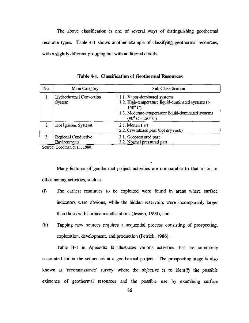
The above classification is one of several ways of distinguishing geothermal
resource types. Table 4-1 shows another example of classifying geothermal resources,
with a slightly different grouping but with additional details.
Table 4·1. Classification of Geothermal Resources
No. Main Category Sub Classification
1 Hydrothermal Convection 1.1. Vapor-dominated systemsSystem 1.2. High-temperature liquid-dominated systems (>
1500 C)1.3. Moderate-temperature Iiquid-dorninated systems
(900 C - 1500 C)
2 Hot 19ueous Systems 2.1. Molten Part2.2. Crystallized part (hot dry rock)
3 Regional Conductive 3.1. Geopressured partEnvironments 3.2. Normal pressured part
Source: Goodman et aI., 1980.
Many features of geothermal project activities are comparable to that of oil or
other mining activities. such as:
(i) The earliest resources to be exploited were found in areas where surface
indicators were obvious, while the hidden reservoirs were incomparably larger
than those with surface manifestations (Jessop, 1990), and
(ii) Tapping new sources requires a sequential process consisting of prospecting,
exploration, development, and production (Petrick, 1986).
Table B-1 in Appendix B illustrates various activities that are commonly
accounted for in the sequences in a geothermal project. The prospecting stage is also
known as 'reconnaissance' survey, where the objective is to identify the possible
existence of geothermal resources and the possible use by examining surface
86
manifestations and undertaking limited field surveys. The activities determine the
boundaries of the prospect area and estimate its potential size.
The exploration stage involves activities to obtain information on the
characteristics of the resource, which include drilling some exploratory wells of 1,000
3,000 meter depths. This stage would detennine the existence, size, quality and
productivity of geothermal resource in the tract. This will allow the investor to infer the
cost requirement for taking the resource out from the ground. Favorable results of an
exploration stage may lead to a development stage.
During the development stage, more wells (called production wells) need to be
drilled. Further activities include establishing necessary facilities to extract the
geothermal energy as well as to prepare for its subsequent designated use such as
constructing the power plant to convert the thermal energy into electricity.
In geothermal electricity projects, both field and power plant developments shall
be completed at the same time. Since field development may take longer time than
power plant construction, the latter action may start after some development progress is
underway. A completed development stage provides the required facilities to produce
electricity from geothermal energy.
4.1.2 Geothermal Utilization
At year 2000, almost 100,000 GWh geothermal energy were in use worldwide.
The statistics shows that a little bit more than half of its utilization worldwide is in the
form of heat. In contrast, the figures for developing countries indicate that more usage is
in the form of electricity (Michaelowa, 2001).
87

Geothermal resource that is used for electricity generation typically has water
temperature of above 1500 C. However, it is also possible to produce electricity from
geothermal waters of 1000 C such as at the Wendell-Amedee in California (Wright,
1998).
A geothermal electricity system is simple, safe and adaptable with modular (1-50
MWe) plants. The modular characteristics of geothermal plants can support the
reliability of an electricity grid system, as well as electrify remote areas where the grid is
not yet established (Mock et al., 1977).
Lower-temperature geothermal resources are used for direct heat applications.
Commercial uses of this type include drying, ore-leaching operations, greenhouses, and
district heating system. In addition, other forms of utilization such as domestic heating,
bathing and cooking were known long before the commercial uses mentioned above.
4.2 GEOTHERMAL IN INDONESIA
4.2.1 Resource Potential
Geothermal energy is one of the indigenous energy alternatives of Indonesia. The
country is located at the junction of three major plates of the earth's crust, namely the
Pacific, India-Australian, and Eurasian Plates. This condition results in a significant
amount of geothermal manifestations such as volcanoes and hot springs all over the
country. The chain of volcanoes along Surnatera, Java and other large islands (except
88

Kalimantan) is known as part of the so-called 'Pacific Ring of Fire'.16
Figure 4-1 shows the locations of geothennal prospects and existing commercial
fields throughout Indonesia, while Figure B-1 in the Appendix details their names and
respective locations.
JNDONESIANOCEAN
PACIFICOCEtW
PhilpPine S8a
INDONESIA
,ds
O~N
l1dE
l1dE
Figure 4-1. Geothermal Locations in Indonesia
Table 4-2 indicates the classifications and estimated size of identified geothermal
prospects in the islands of Indonesia. The proven, probable and possible potentials are
estimated to be around 20,000 MWe. Almost half of the potential is located in Sumatera
and nearly 30% is in Java. This means around 80% of the resource potential is located in
26 The terminology refers to the chain of volcanoes that was created by the upward intrusion of magma(molten rock) at the edge of the Pacific Plate. The 'ring' extends along the west part of the Americacontinent, the Aleutian Islands. Japan. the Philippines. Indonesia, the South Pacific and New Zealand(Wright, 1998).
89

the islands that are home for 80% of the country's 206 mi1lion population,27 which means
that geothermal resources are located near the demand centers.
Table 4-2. Geothermal Resource Potential in Indonesia
Classification* # of Prosnect Locations Size (MWe)
Proven 7 Java (4), Sumatera (2), Sulawesi (1) 1,192Probable 14 Java (9), Sumatera (3), Sulawesi (I), Nusa 2,250
Telll"lmra (I)Possible 55 Java (26), Sumatera (21), Sulawesi (3), Bali 14,089
(I), Nusa Tenl!l!ara (2), Maluku (2)Hvnothetical 55 6,132Sneculative 162 36,500Note: * From top to bottom, the list mdlcates a decreasmg degree of certamty that reflects the
quality and quantity of available information on geothermal system at the prospects.Refer to Table B-1 in the Appendix for additional explanation.
Source: Directorate General of Oil and Gas, 1996
Compared to 20,761 MW capacity of the existing power plant under the
management of PT. PLN (the National Electric Company),28 geothermal resource
potential is obviously an important alternative energy source to support the system.
Large resource potential and favorable locations are important advantages of geothermal
energy in Indonesia.
4.2.2 Resource Utilization
The Government of Indonesia (GOl) encourages geothermal development as part
of the energy diversification policy, which among others is intended to ease the pressure
of domestic demand for oil. The national energy policy as well as the existing regulation
27 BPS Slatistics Indonesia for year 2000. (http://www.bps.go.idlsector/popnlationltableI.shtml)2' As of year 2000, the total installed generating capacity in Indonesia was 37,591 MW and PLN owns 69%of them. (Statistik Ketenagalistrikan, hup:/Iwww.djlpe.go.idlinformasilframe_informasUistrik_2.htrn)
90
categorize geothermal as renewable energy. For small power producers, the energy
diversification policy leads to a favorable regulation that dictates a higher priority for
power supplies that uses renewable energy including geothermal plants. In large power
supplies division, geothermal plants have been regarded as 'must run' suppliers to the
system that indicates the highest priority in the dispatch order.
Despite those favorable conditions, however, progress of geothermal utilization
has been very slow. After more than a decade of development, direct application is
limited to traditional use and few experimental projects. The commercial geothermal
utilization is only for electricity generation, which is supplied by three geothermal fields
with total installed capacity of 525 MWe.
A major disadvantage is the fact that electricity from some geothermal projects
are presently more expensive compared to other types of electricity generation in the
country. There have been a lot of discussions as to whether or not other energy sources
h b . d'~'1,29ave een pnce ,atr y .
Nevertheless, several factors have contributed to the high price of geothermal
electricity. One reason is a high cost that, among others, relates to inherent difficulty in
finding and extracting the energy from the earth that requires special technology and
skills as well as adequate financial support. The project requires high initial capital to
gatber information about the underground reserves as well as to construct the operation
facilities. In addition, field works and power plant construction may use up three to
2. Petroteum-refined fuels have been heavily subsidized, although the government is currently attempting todecrease the subsidy amount. In addition, there has been some concern on the pollution effects of coal andoil, as well as the economic consideration that oil and coal can be exported. Hence, some additional costs(externality and opportunity costs respectively) in comparing coal and oil to geothermal have to be takeninto account.
91

seven years of the project life before any revenue is generated. As such, geothermal
development project is a highly specific investment with large capital outlay and long
preparation time.
The second disadvantage is the 'non-transportable' nature of geothermal energy,
which requires the location of power plant on site or nearby the field. Further,
geothermal potentials are commonly found in remote locations with lack of transmission
and distribution network. Consequently, these conditions associate such geothermal
potentials only to the small local market.
The third shortcoming is that there is no mechanism to effectively represent
significant benefits of geothermal development, such as the long-term low cost of
operation, low emission of pollutant particulates, and the impacts of diversification of
supply from an indigenous, distributed resource (US Embassy, 2002).
Another complication arises from an unfinished process of regulatory reform. In
contrast to the previous oil and gas law, the new law that was promulgated in October
2001 excludes geothermal. The problem is that the special regulation for geothermal
utilization has not been put in place.
4.2.3 Business Environment
This study focuses on so-called geothermal total projects. This terminology is
used by the GOI to refer to geothermal projects where the same investor (or consortium
of investors) is responsible for both the developments of geothermal field as well as the
92

electricity generation. 3o The final output of an investment in geothermal total project is
electricity; therefore the explicit price for output is only for electricity.3!
Figure 4-2 shows advancement in a geothermal electricity project in Indonesia.
Previously, the GOI would provide an estimate on reserve potential and other preliminary
data based on some limited surface surveys on the prospective site. In contrast, the
Presidential Decree 76/2000 requires more GOI work at this stage, i.e., until the search
concludes whether or not the prospect can be upgraded into the 'probable' status. 32
A proposal that expresses an interest to pursue a geothermal project would include
a work plan and a price of electricity to be produced by the project. Once the contract is
signed, the investor's tasks in developing the field closely resemble those in oil projects.
However, in addition to developing the field, investors would need to develop power-
generating facilities as well. The production stage starts following the completion of
field development and power plant construction.
TTl Start Development I
Negotiation Exploration Development
Start Production
1_.to t2 time
Figure 4-2: Progress in a Geothermal Project
30 Contrast this to the case where field development and power generation are independent projects ormanaged and operated by different parties.31 If field development and the construction of power generation are independent projects, the output willbe stearn from one project and electricity from the other. In this case, output price will refer to steam pricefor the former and electricity price for the latter.32 The probable status is determined based on the information from drilling at least an exploratory well.
93

As highlighted in Chapter 1, the economic crisis that started in 1997 had raised
concerns over the role of private participation in the electricity sector. Some of the
suspended projects are renegotiating their terms and conditions with PLN, while others
choose to enter the arbitration procedure. The problem has been more complex in
geothermal development, because unlike other private power generations, private
geothermal project involves the utilization of natural resources. Similar to all natural
resources in the country, geothermal resources belong to the state?3
Based on this view, Presidential Decree 45/1991 determines that private
companies may participate in geothermal development as contractors to Pertamina, the
state oil and gas company. A Joint Operation Contract (JOC) governs this relationship.
Further, Pertamina or the JOC sells either steam or electricity to PLN or other parties for
electricity generation. An Energy Sales Contract (ESC) governs the purchase of
electricity by PLN, which is usually denominated in dollars and includes a take-or-pay
clause. The decree also includes a favorable tax treatment that lumps all applicable taxes
into an income tax rate of 34%. Under this arrangement, a severe exchange rate
depreciation following the economic crisis has caused enormous financial burden to PLN
andGOI.
Presidential Decree 7612000 was promulgated in May 2000, introducing a new
arrangement for private participation in geothermal development. In an effort to improve
the initial information for starting geothermal projects, the decree positions the Gar as
the exclusive party to conduct exploration activities in determining probable reserves.
J3 Article 33 of The Indonesian Constitution of 1945 stated that all naturat resources are under the power ofthe state, which shall manage those resources to the greatest benefit of the people.
94
Private corporations can develop geothermal resources for their own use; or if the
development is to generate electricity for public use, then they shall proceed under
cooperation with PLN. Hence, this arrangement no longer includes Pertamina. Further,
the decree states that the electricity prices shall be denominated in Rupiah and removes
the one-for-all tax rate by stating that this activity is subject to regular income and other
taxes. Although this decree does not affect geothermal project agreements signed prior to
May 2000, the existing corporations have been trying to convince the GOI to revise the
decree. At the same time they are actively involved in proposing inputs to shape the
forthcoming geothermal law.
The above description illustrates the dynamic changes that are taking place in
geothermal development. In addition to the regulatory adjustment mentioned above, the
following list shows various factors that form a unique business environment and may
contribute to the delays of geothermal investments in Indonesia:
a) Legal and Institutional Framework:
Geothermal electricity production involves field activities that are similar to other
natural resource extraction activities such as oil and gas or other mining works.
Furthermore, the project also includes electricity production. At present, mining and
electricity generation are governed by separate groups of regulation. A potential may
arise from a longer bureaucratic process such as for acquiring various permits with
respect to individual activities; or different applicable taxes as a geothermal total
project involves both activities. This situation is prone to conflicting issues and
therefore is insecure.
95
b) Risk Allocation:
i) Proposal and Negotiation Stage:
• To submit a proposal, private fIrms have to rely on information made
available by the GOl. Under the Presidential Decree 45/1991, information
about the tract that is generally based on reconnaissance (surface survey)
data only. The Presidential Decree 76/200 requires that at least the
reserves are offered to potential developers in a 'probable' status.
However, limited government budget may suggest that there will not be
many geothermal sites available for development in the near future.
• The fIrm would have to propose a price for the output (electricity) in their
project proposal, which is a pre-requisite to go to the negotiation table in
obtaining the concession area. The negotiated price will be stated in the
contract. This means fIrms are required to determine part of their project
return ex-ante, regardless of limited initial information and uncertainties
they must encounter (reserve size and productivity, demand size, the price
of other energy in the future).
ii) Exploration Stage:
• To better assess the resource potential, companies will need to undertake
exploration activities that includes the drilling of at least 3-5 exploratory
wells. This activity may take 3-5 years. Investors have to devote quite a
sum of money, since each drilling for preparing a production or injection
96

well would cost $1-3 million.34 The exploration results indicate whether
or not to proceed with development, and at what cost.
• As the consequence of the high uncertainty on the exploration results,
external funding is likely to be expensive.
iii) Development Stage:
• In a geothermal electricity project, the development stage covers the
development of the field as well as the construction of the power plant.
Moreover, both activities are to be conducted in such a way that they will
be completed at the same time. The amount of capital to be invested here
is therefore much larger when compared to projects that prepare either one
of them separately (i.e. the geothermal field or the power plant only).
iv) Production Stage:
• Only one buyer:
The prevailing regulation states that a geothermal electricity investor, like
other Independent Power Producers in Indonesia, can sell their electricity or
use it for self-consumption. Although the regulation allows private generated
electricity to be sold to both PLN as well as to any other buyers, the
transmission system is owned by PLN and there is no legal base allowing the
use of this system by parties other than PLN themselves. Other potential
consumers or the investors themselves may be willing to build the
transmission and distribution facilities. However, the following constraints
34 Mock, Tester & Wright, 1997. The figure is in 1994 US$.
97

prohibit this alternative to be pursued, at least for some time in the future.
The first problem emanates from the existing regulations that grant the
exclusive rights of ownership and management of electricity transmission and
distribution system to the state. Even if this restriction is lifted, the second
problem is the economic justification for this additional capital requirement.
A certain size of demand would be needed to warrant the economic of scale of
this investment, since it would need a significant additional capital on top of
the huge investment of the geothermal system itself. Therefore, in practice
PLN is the only buyer for privately generated electricity.
• Limited market:
The utilization of geothermal resource is site-specific. If the energy is
converted to electricity, it can be delivered to the nearest grid system and
therefore can reach distant demand areas. Nevertheless, the electricity
generation facility itself is usually in the vicinity of the reserve area.
Especially when compared to oil and gas (in the form of LNG or NGL), which
can be transported abroad and traded in the international markets, geothermal
resource utilization is bounded by their location.
c) Return on Investment:
(i) The project is characterized by a fixed-price contract, since the output price is
determined ex-ante for the life of the project. This type of contract puts the finn
in a position where it bears the entire loss when there is cost-overruns, as well as
98

enjoy the whole profit in the case of cost-underruns. 35 However, when the project
starts, how much money to be spent is as uncertain as the status of the resource
size, quality, and productivity. Thus the ex-ante negotiated output price does not
guarantee that the investors will recover their costs and that the decision to take
the project is worth the risk.
(ii) The above conditions may be economically acceptable for private firms, as long
as they can have a return that covers all the expenses and provide a positive yield
comparable to other investment opportunities with similar risks. In other words,
investors are willing to take the risks if the payoff is sufficiently large. This
implies that the more risks left to the investors, the more expensive the output
price will be. On the other hand, one of the present problems in the business is
that PLN, which is the only buyer, is reluctant to purchase geothermal electricity
because of its higher price relative to electricity generated by other types of
energy such as hydropower, coal, and oil.
d) Economic Condition:
The lengthy economic crisis that was started in 1997 has caused the currency to
depreciate significantly. From Rp.2,500 per US$ then, it has been fluctuating in the
range of Rp.8,000-1l,000 per US$ during 2002. A continuing major problem is the
substantial external debt of the public as well as private sectors. These debts leave
Indonesia exposed to interest rate and exchange rate shocks, which implies
macroeconomic vulnerability.
3S David, A K and Wong, K (1994)
99

All the above conditions illustrate the complications that restrict further progress
in geothermal development. Considering that there are very limited commercial
geothermal sites at present, some significant changes need to be contemplated to
encourage further development.
4.2.4 Perspective for Modeling
As illustrated earlier, adjustments in a larger framework of regulatory setting are
underway, along with the general issue of restructuring the economy. Correspondingly,
some alternative arrangements for geothermal project development had been discussed.
It is acknowledged that the changes need to balance the risk and reward for both the
GOIIPLN and the private investor. Skilled professionals as well as significant capital
requirements to develop geothermal fields are certainly important factors for this venture
to be successful. Nevertheless, it is equally important for the proliferation of geothermal
resource utilization that the project bears acceptable attributes such as competitive price
as well as good quality and reliable supply.
Among the above host of issues, this research focuses attention at the geothermal
project itself and less emphasis on the atmosphere. Further, the research concentrates on
the significance of natural characteristics of geothermal resources to the project. The
benefit of restricting the interest span is to help isolate some inherent issues specific to
geothermal electricity projects. On the other hand, a drawback of this approach is an
unclear picture of the findings impact on the utilization of geothermal energy resources of
the country, since the latter also depends on various other factors beyond the project
boundary such as investment climate of the economy. Nevertheless, the research findings
100

point toward specific ways that can be used to facilitate the transaction process between
the government and potential private developers.
The costs of geothennal project are highly site and project specific,36 implying
that the economics of geothermal energy extraction are highly variable and wide-ranging.
The natural condition of the reserve is one of basic features that affect the other project
characteristics. For this reason, this research focuses on the use of better infonnation
about the natural characteristics of geothennal resources to the overall project valuation.
36 Major factors to the costs of geothermal power development are temperature and depth of the resource,type of resource, chemistry of geothermal fluid, permeability of the resource, plant size, technology of theplant, infrastructure requirement, climatic condition of the site, topography of the site, environmentalconstraints, proximity of transmission lines, construction contract, and indirect costs that includesadministrative costs, management costs, insurance, permits, financing, taxes, and royalties (World Bank,http://www.worldbank.orglhtmllfpdlenergy/geothermalJassessment.htm#economic)
101

CHAPTERS
THE VALUE OF INVESTMENT OPPORTUNITY
This chapter describes an evaluation process for a hypothetical geothermal
electricity project using both the conventional DCF approach and the real option analysis.
During the conventional DCF analysis, the model setting resembles the present project
conditions in Indonesia, where price is set ex-ante and fIxed for the project life regardless
of the results of the exploration phase. The real options analysis considers the impacts of
incorporating some flexibility to the base model.
The fIrst part of this chapter discusses project features through the use of two
DCF fInancial assessments, as these forms of presentation are more widely used. In
addition, the methods embrace relevant project information useful in building a case in
real options analysis (ROA) setting. The purpose of this section is to further introduce
the project structure prior to instigating the real option framework into the analysis.
The second part of the chapter presents the implementation of a real option
approach. The project is portrayed as sequential compound options. Copeland and
Antikarov (2001) option valuation technique is used, such that the lack of market
information does not hamper the application of the theory. The procedure highlights the
presence of flexibility in management decisions that are inherent in such structure, and
shows that it is indeed valuable. Recognizing such flexibility is appropriately important
so that they can be utilized accordingly. A particular interest in this exercise is to
examine the relationship between the additional project values to lowering the output
price.
102

Figure 5-1 outlines the interrelationship of research components. The fIrst step is
to structure the problem in influence diagram form, fill in the payoff values and calculate
the net present value of the project without flexibility. The second step is to examine the
project value at the good state, which is the state where exploration is successful and the
project enters the production or operation stage. The volatility of the project value
(parameter z) is estimated using Monte Carlo simulation. The third step is to generate the
structure of the compound options and calculate its value.
The presence of user friendly yet sophisticated modeling and computational
software for personal computers provide the means to represent unique characteristics of
individual real investment problems as well as perform meticulous numerical exercises of
lattice approaches. The exercise involves integrating the utilization of two commercial
softwares and two computer models.
The commercial softwares are Microsoft Excel that is used as a platform for the
two computer models, and DATA™ (Decision Analysis by Treeage)37 that is used to
construct the structure of the research model in influence diagram format. The two
computer models are GEM (Geothermal Electricity Model)38 and the Compound Options
model. The fIrst model is a fInancial model for geothermal project, which takes into
"Decision Analysis by TreeAge (DATA) version 3.5 is a trademark of TreeAge Software, Inc.lS Electroconsult of italy built the original GEM in Lotus for the Directorate General of Electricity andEnergy Development of Indonesia in 1996. The model utilized in this research is tailored to accommodatethe research needs. Changes include conversion into Excel, revision ofsome formulas and incorporation ofadditional features to facilitate the linkages to other research components.
103

Monte Carlosimulation
i
tVar (2) I•
I•·
:I
Good state I ~.L. • NFV• _ • _ • _ • _ • _ • _ • _I. _ • _ T _ • _ • _ • _ _. _ • _ • _. •
. Changeinput~
.------, I probability form,Intermediate calculations i : range of value
Inflation Projected FCF (nominal)
IProjected FCF (real) i.-.-.-"-.-.-"-.-.-1-.-.-.-"-"'(;Ej\,," -"
I Model and value the Compound Options I"
........................................., ~~~~~..~~~~.~~ £i ~:~~ea: ~ i1
.......................................................... " .Excel DATA™
Figure 5-1. Research Outline
104

account field development as well as power plant operations. The second model is
developed following the technique introduced by Copeland and Antikarov (2001).
Steps 1 and 2 of the research procedure integrate the utilization of GEM and
DATA™. Step 3 uses GEM and the Compound Options Model to obtain the price
implications and the option values. The exercise considers a hypothetical geothermal
prospect located in West Java. The description below uses a corporate point of view
since the developer is assumed to be the party that undertakes the activities.
Nevertheless, in essence it can be seen as an investment decision problem by either the
government or the developer.
5.1 NET PRESENT VALUE ASSESSMENTS
A preliminary government study estimates such prospect has a 110 MWe
potential capacity. The nearest transmission grid is a few kilometers away, and there are
several small cities and industry complexes around the district. This prospect seems very
attractive, however the project proposal would need a careful examination since it
involves a large initial capital outlay and several years to complete the facility.
Moreover, the present regulation does not allow private companies to sell electricity
directly to consumers. Rather, it has to be sold to the state utility company, which would
buy only if their price could compete with other electricity generation companies. The
future price of electricity produced by the facility has to be determined before the project
starts. For this purpose, the project profile is estimated based on available information.
105

The fIrst part of this section identifIes project components and their interrelationship,
while the second part incorporates available data and information into the structure.
5.1.1 Model Structure
Figure 5-2 illustrates the prevailing system of geothermal development,
highlighting the interrelationship of project decisions and major variables affecting such
decisions in an influence diagram representation. A brief note about the components of
this model structure and interrelationship among them are illustrated below. A more
detailed description can be referred to section C.7 of Appendix C, which also contains
background information about influence diagram and its symbols.
D3:Develop?
C2,Exploration
CI:Negotiale
Terms
DI,Invest?
Figure 5-2. Uncertainties and Major Decisions in the Base Case Model
106

There are three major decisions to be made, which are indicated by rectangles on
the picture: (i) whether to invest in the venture, (ii) whether to continue with exploration
after the negotiation on project terms is concluded, and (iii) whether to continue with
field and power plant development, which leads to electricity production. The ovals and
circles represent uncertainties surrounding the resources existence and characteristics, the
project terms to be negotiated, the outcome of the series of activity to learn about the
reserves, and the actual sales of electricity. The double-lined circles stand for
deterministic variables, which are parameters that have a single, fixed value in the model.
The hexagons symbolize a group of deterministic nodes that belong to the same logical
group, incorporated to simplify the diagram appearance. The arrows indicate flow of
influence among the nodes.
No arrow pointing toward node C4 indicates that the actual size and condition of
the reserve capacity will never be known with certainty. However, its size can be
estimated by conducting a series of studies. The government or a third party conducts the
reconnaissance survey. When such survey indicates that the area is prospective (node
FI), this result becomes the primary information for the government to invite potential
investors. The company has no control over such forecast or estimate figures; hence
there is no arrow from any decision node into node FI. In contrast to FI, the company
controls the other two studies at node C2 and C3. The order of occurrence of FI, C2 and
C3 reflects time sequence and quality of results. A later study would yield more accurate
estimate, but at a higher cost.
107
A contractual negotiation takes place after a decision to pursue the investment
opportunity, but before any field activities commences. This negotiation would yield a
certain pricing and supply figures embraced by node Cl, which is set for the lifetime of
the project. The arrows emanating from Cl into D2, D3, C5 and C7 show direct
influence of this agreement, while it indirectly influences C2 and C3 through D2 and D3
respectively. The amount of sales and the accumulative expenditure during the
preparation of geothermal field and power plant facilities would dictate the total value of
the project.
Table 5-1 summarizes the classifications underlying the use of arcs on the model
structure. The use of DATA™ 3.5 allows exclusion of some arcs, such as those assigned
for the 'no-forgetting property' ,39 because the software has an internal mechanism to
automatically recognize an appropriate structure. However, Figure 5-1 presents the
whole sets of these arcs for the general readers.
5.1.2 Information and Data for the Base Case Model
(a) Data Sources
Data on the Indonesian geothermal electricity projects are obtained from the
following sources:
(i) Directorate General of Geology and Mineral Resources: a map depicting locations
of geothermal prospects in Indonesia.
39 Refer to Appendix C for description of this terminology.
108

Table 5-1. Notes for The Arcs'
Reason for arc assignment Relevant nodes
Cost components of ROI calculation
_~illgl~~,,£isi~:_~J.e~~prop~~_~yb________________________ _ P!_2.I:l_:?_::?_P_L _No-forgetting property' FI -7 D2
FI -7 D3I-:--------:------;----~---------------:-_::-- --;-- --:---------;;-;:------------------ -------- ----------- ----t--------------------------------------
Imperfect information (in the form of forecasts, C4 -7 F1estimates, or tests) that will be used to represent the true C4 -7 C2~~tt;,_~_\ll.':t; thel'_3:~~g~S_t;~\'~_t;_~r_l_i~~_________ __ S'!±.<;L_______ __Input for a decision F1 -7 D1
CI -7 D2C1 -7 D3C2 -7 D3_._._-_._._---_._----_._._.,..,-_.,.._._._._.~--_._._- •.•.•.•.•.•.•.•.•.__.•.•.•._.•.•._--.,.-.,....... .....•.•.•.•,.".--_.__.__.•.•.•._-_.•.•.•.•.__...._-_.•.__._-_._-_...... ' ............•----.-."",--_._-_.FI-7 C6C2 -7 C6C3 -7 C6C5 -7 C6._-----_.__._--,-."-- _._.~_.__._----_._--_.__._---"_._".,_._._._._._._.-..,._.-.--.'.-.•._--------_ __.•.----.".-.,.,..•.•.•.-.•.•.__.•._,-_._------
Revenue comoonent of ROI calculation C7 -7 Ra Specific description, in addition to the generic remarks stated on Table C.2. Pairs ofnodes and arc that are not listed only have the applicable generic remarks.bDefinition1-(ii), Section C.2, Appendix C'Defmition I-(iii), Section C.2, Appendix C
(ii) Electroconsult et al. (1996):
The final reports On Geothermal Private Power Development project for the
Directorate General of Electricity and Energy Development of Indonesia, m
particular the following parts of the set:
• Geothermal Electricity Model, which is a financial model for geothermal
project in spreadsheet format and the respective user's guide.
• Evaluation Technique, which is a guideline to assess investment proposals
from private investors.
109

(iii) Enerindomumi (1999):
Final report of Studi Pengurangan Resiko Eksplorasi dan optimasi Pembiayaan
Pengembangan Panas Bumi (study for exploration risk reduction and geothermal
development cost optimization), for the Directorate General of Oil and Gas of
Indonesia. The report provides average figures of qualifications and general
characteristics of Indonesian geothermal prospects. The report also includes a
simulation model named Sistem Analisa Resiko (SAR, risk analysis system),
which contains database of several Indonesian geothermal fields.
(iv) Indonesian Geothermal Association: files describing the present business structure
and ideas to improve the sector's condition.
(v) Ministry of Mines and Energy: contracted prices of geothermal projects.
(vi) PLN: load duration of Java-Bali system in 2000.
(vii) US Embassy Jakarta (2002):
A report on Indonesia's geothermal development, which is the source for
contracted prices data and the status of geothermal development projects.
(viii) Other sources:
• Web pages on financial parameters, options, and geothermal.
• Articles by Indonesian scholars and geothermal practitioners concermng
generation costs of various power plants and ideas to improve the present
condition.
• Personal interviews concerning financial indicators and country performance
in financial market.
110

(b) Electricity Demand
The national demand for electricity has been growing at an average of 14% per
year since 1985, as shown in Figure 5-3. This growth rate is expected to continue for the
next couple of decades, considering the existing electrification ratio of 53%.40 In
addition, the prolonged economic crisis has caused infrastructure development to slow
down significantly, which adds more pressure to the unfulfilled demand potential for
electricity. Therefore, future demand is expected to be strong.
25%
20%
15%
10%
5%
0%
......,----/,.-
rI+- ..f--t
80
60J::
40 ~..20
o85 86 87 88 89 90 91 92 93 94 95 96 97 98 99
Year
1_Annual Growth --+- 8ectricty Consurrptkm 1Source: Biro Pusal Statislik, 2002.
Figure 5-3. Electricity Consumption
(c) Reserve Potential
The presence and size of economically feasible reserve in the prospect area is yet
to be studied. Initial information from surface examination is not a reliable estimate,
40 Ariati (2001)
III

since among others, geological structure and hydro-geological conditions beneath the
surface have a major influence on the feasibility of the prospect. This uncertainty can be
resolved only by investing in a series of activities to study the underground
characteristics of the geothermal system in the area, which requires drillings of some
wells.
(d) Project Time Plan
The examination and preparation period would take about five years. Exploration
surveys and drilling activities would need one year respectively, while the development
of both the fields and power plants requires three years. The lifetime of the completed
facility is estimated to be 35 years, where a full capacity operation is expected to take
place during the first 30 years and a declining capacity during the last 5 years of its
lifetime.
(e) Estimated Costs
The initial estimate indicates that the geothermal potential under study has a 110
MW potential capacity. As a reference, the unit costs for various types of geothermal
project in developing countries are shown in Table 5-2, which indicates that the total cost
per unit of power generated by the facility is likely to be in the range of US$2.5-6.0
cents/kWh. However, the capital costs of geothermal projects are highly site and project
specific (World Bank, 2002). Some information on the average costs of geothermal
project in the country may provide additional information.
112

Table 5-2. Unit Cost of Power
US centslkWhHigh Quality Medium Quality Low Quality
Resource Resource Resource.8.J!lll1l P~l1tsJ~MF-.L_._._. __ __ ..?:.Q.:}:Q_ _ ?:?=_~:.?__ __ __.__~.O -::ISlJ_.. ._~edi!'m.J>I~l1ts(5:}QMF2..~:Q.=~:2._.. ±:?.=_?:L_._ ~g!~!!y. n()t.~!:'.i.t.~!?!"' __ .Lal"~e Plants (>30 MW) 2.5 - 6.0 4.0 - 6.0 Normallv not suitableNotes: Assume 10% discount rates and 90% capacity factor.
Estimates are based on geothermal projects in developing countries, where indirect costs are at thehigher end of the scale.
Source: World Bank, 2002.
The following cost estimates are based on the Indonesian figures reported by
Electroconsult (1996), The economical size for the best available. technology at the
moment calls for a minimum of 55 MW commercial power generation capacities. This
implies that the facility needs two 55 MW electricity generating units, which would cost
US$95 million in total.
The company needs to do some fieldwork to examine the available resource
potential, as well as develop the fields to supply the power plant of the planned size. The
fixed costs of this project are estimated to be US$3 million for surface exploration and
studies, and U5$5 million for establishing land access and rights.
Usually a project of this size requires 5 exploration wells that cost U5$2.3 million
each. At least 3 good exploratory wells are expected to be good enough to be used as
production wells. Historical company performance suggests lbat their success in drilling
can be represented in a ratio of productive to unproductive well of 4 to 1, provided that
the area contains the amount of energy as estimated by the government.
Assuming that the average initial performance of production wells is 7 MWe and
the required reserve capacity is 5% of the full capacity, this facility would need 16.5
113

production wells to supply the 110 MW power plants in its first year of operation.
However, the 4: 1 drilling performance suggests that the company would need to drill 22
wells to obtain the necessary supply of geothermal energy. The unproductive wells are
commonly used as re-injection wells, and one re-injection well is required for every three
production wells. Although the cost of a development well is not as much as an
exploration well, the expenditure is still significant. The company expects to spend
US$1.5 million per well.
In addition, the company estimates that the well productivity rate could decline at
2% per year. 41 Therefore, during the operation stage the facility needs additional drilling
of the so-called 'make-up' wells to maintain the rate of steam supply to the power plant.
The company plans to drill one make-up well every two years, and the estimated cost is
US$1.5 million per well.
A gathering system is required for connecting productive as well as make-up
wells. The establishment of this system is estimated to be around US$O.72 million for
each productive well, and US$O.38 million for each make-up well.
Administrative and engineering costs during exploration and development are
around 10% of investment costs, while during operation it is estimated to be 10% of
yearly costs. Operation and maintenance costs during operation are estimated to be 2%
of total investment.
41 In this respect, geothermal resource is not renewable. Exploitation triggers certain physical and chemicalprocess underground, and added to naturally occurring process, will lead to depletion of the geothermalresources (Dickson and Fanelli, 1995). Mock et al. (1997) views geothermal as renewable in the sense thata complete recovery of original temperature will occur within a period ofless than 10 times the productionperiod.
114

(0 Financial Parameters
The company also incorporates the following parameter values in the investment
proposal:
• 20% discount rate for both field and power plant developments and a 30% target for
the return on equity. The discount rate figures over the past decade are shown in
Figure 5-4. Erb et al. (2002) calculation shows that based on credit ratings that reflect
the systematic risk of the country, the expected return for average risk investment in
Indonesia range between 21 %-25%. Since geothermal project is considered risky, as
also supported by the common observed rate used by business participants, the
minimum ROE for this model is set at 30%. Economic crisis, unsettling political
issues, weak law and regulatory enforcement, contract breaching and financial
difficulties in numerous power projects, as well as less international involvement in
the Indonesian financial market has led to high premium requirement for capital
investment. Some disruptions and instabilities in the trading of government bonds
during recent years led to inactive trading, suggesting that the bonds may not be used
as an indicator for country risk anymore.
• Funding during exploration period comes solely from the shareholders, since high
degree of uncertainty on project existence during its initial stage commonly
discourage commercial lenders to participate in the project. During the development
stage, the majority of capital requirements shall be funded from commercial loans.
The total equity funding during exploration and development is 40% with minimum
115

30% rate of return. Conunercial funding is estimated to bear 8% interest in constant
value and payable in 10 years period.
50%
40%/\30%
/' \.20%~ ~ j V
10% ..0%
90 91 92 93 94 95 96 97 98 99 00 01 02
Year
Source: Bank Negara Malaysia, 2002.
Figure 5-4. Indonesia Discount Rates
• Income tax rate and royalty are 30% and 4% respectively. Presidential Decree No.
76/2000 promulgates a new tax rate replacing the 30%-4% pair. This model uses the
previous tax and royalty settings since this exercise is used later to compare this
model with the existing business arrangement. Moreover, a draft of geothermal law,
which is of higher legal status than the decree, is currently being prepared. This
activity indicates that the decree may not be sustained. Further, there has been no
new geothermal projects following the promulgation of the new decree.
116
(g) Estimated Revenue
Assume that scheduled and non-scheduled maintenance would reduce plant
operation by 10% of its gross capacity. This means power plant availability is 90% of its
gross capacity ('gross availability factor', OAF). Additional downtime due to lack of
system demands and economic dispatch considerations is estimated to cause the plant
runs at 85% of its availability factor ('discretionary factor', DF). Further, internal
electricity consumption for the power plant and field operations is estimated to take
around 5% of its gross energy production. Taking all these factors into account, the
facility is expected to sell 700 OWh42 per year throughout its full-production period of 30
years.
The payment of purchase consists of several components. They are 'generation
component' that relates to generating capacity of the facility, and 'resource component'
that reflects the amount of energy sales during the period. In other words, the first part is
the fixed components and the second part is the variable components of the price. In
addition, there are operation and maintenance charges attached to each of these
components.
As previously indicated by Table 5-2, the initial estimate for the output price of
the project is between US$2.5-6.0 centslkWh. However, subsection (f) shows that the
project uses higher discount rates and lower capacity factor than the level used to
construct Table 5-2. Therefore, it is likely that the price range for the project is skewed
42 (110 MW x 8,760 hours per year x GAF x OF x (I-internal consumption))/l,OOO
117

toward the upper range of the World Bank estimates, and probably more than US$6.0
cents/kWh.
There are many values of the price components that can produce a unit cost of
around US$6.0 cents/kWh. The Base Case in this exercise uses the figures calculated by
Electroconsult (1996), which is in line with the World Bank figures plus the above-
mentioned adjustments. Based on the expected return on equity (ROE) target of 30%, the
following example of input set yield a unit cost of US$6.19 centslkWh and is used as the
benchmark figures for the other scenarios:43
• Capacity Charge Rate (CCR):
• Operations and maintenance for CCR:
• Energy Charge Rate (ECR):
• Operations and maintenance for ECR:
US$20lkW per month
US$2lkW per month
US$0.0331/kWh
US$0.0071/kWh
In addition to the above pricing terms, one must consider an additional stipulation
that specifies a minimum amount the utility is required to purchase. Usually referred to
as the 'take-or-pay' (TOP) clause, it says that if the purchase were greater than the TOP
level then the company would offer to reduce the ECR by 50% for the extra purchase.
However, if the purchase is lower than TOP then the company still receives payment for
the TOP amount. Based on the above price figures, the expected revenue from selling
700 GWh of electricity is therefore around $65 million per year.
43 The existing geothermal projects are used as references. Appendix D lists other parameter values thatrelate to this calculation.
118

5.1.3 Decision Tree Assessment
Table 5-3 through Table 5-5 provides additional layers of information to the
influence diagram of project structure shown in Figure 5-1. The tables reflect some
judgments and estimates based on existing similar activities and the assessments of
company experts. These figures may vary among prospect areas and with the knowledge
and expertise of the respective company.
DATA™ 3.5 facilitates the conversion of influence diagram into tree
representation as part of its solution procedure. Modeling the project as influence
diagram structure using the decision analysis software eases the implementation of
Bayes' Theorem in translating the estimates of conditional probabilities in Table 5-1 into
appropriate joint probability figures. The inferred probability interrelationships in the
model can be seen in the form of formulas below some of the tree branches.
The model incorporates the following asymmetry assumptions to exclude
irrelevant conditions and therefore avoids unnecessary branches of the tree:
(i) No investment will take place in states of nature where it makes no sense to
do so.
(ii) If the company declines to invest at node Dl, or does not reach an agreement
at node Cl, or decides not to explore at node D2, or decides not to develop the
field at node D3, then there will be no production of electricity and
consequently no sales.
119

(iii) If the reserve is not feasible, then development activity will definitely result in
'fail' .
(iv) If development activity is successful, then the project proceeds to production
stage.
Table 5-3. Chance Nodes
Node Identifier Possible ProbabilityOutcome
FI External Good info p(Good infolReserve is Feasible) =IInformation Bad info p(Good infolReserve is Not Feasible) =0.5
o(Bad infolReserve is Feasible) =0*CI Negotiate Terms Agree 0.5
Not A!!fee 0.5C2 Exploration Success p(SuccessJReserve is Feasible) =0.7
Fail o(SuccessJReserve is Not Feasible) =0.1C3 Development Success p(SuccessJReserve is Feasible) =0.8
Fail I o(SuccessJReserve is Not Feasible) =0C4 Reserve Feasible 0.6
Caoacitv Not Feasible 0.4C5 Production Production p(Production/Success at Development,
No Production Success at Exploration, Agree on Terms) =0.9
C6 Costs Costs IC7 Sales Sales INote: * Statement (Bad mfolReserve is FeasIble) says that the prospect IS not feasIble.
Regardless of the actual condition of the reserve, the 'non feasible' evaluation resultmeans that the area would not be offered to investors in the frrst place.
Table 5-4. Decision Nodes
Node Identifier Alternatives
DI Invest? InvestDon't invest
D2 Explore? ExploreDon't explore
D3 Develop? DevelopDon't develop
120

Table 5-5. Deterministic Nodes
Node Identifier Value Definition Remarks
Charge CCR 20 Grouped within the "PriceCharge OM CCR 2Charge ECR 0.0331
Terms" sub model
Charge OM ECR 0.0071Reduce ECR 0.5Capacity 110 Grouped within theTOP 0.8DF 0.85
"Quantity Terms" submodel
Inflation 0.03Company Discount Rate 0.2
Utilization of another software product, Geothermal Electricity Model (GEM),
facilitates the calculation of the payoff value for each path on the tree. GEM is a
financial model that takes into account exploration and field development activities in a
geothermal electricity project. Both models are linked in the following way:
(i) The payoff values for various states of the model is calculated in GEM, and
exported to DATA as inputs to calculate the project value without flexibility.
(ii) GEM undertakes necessary calculations to produce the rate of return on project
value, and exchanges the information back to DATA,
(iii) DATA calculates the volatility of the rate of return parameter by performing
Monte Carlo simulation in cooperation with GEM. This procedure asks DATA to
vary the values of several parameters, transfer a new set of values to GEM as
inputs for item (ii) above, and GEM transfer back the results to DATA. This
exercise employs DATA to manage item (iii) for 1000 iteration.
121

Figure 5-5 shows a decision tree that embodies the influence diagram structure in
Figure 5-2 and all of the information stated in Tables 5-3 through 5-5. Figure 5-6 shows
a rollback decision tree which uses expected net present value to find the optimal
decision policy. There is only one possible path with positive payoff and has only 16.8%
probability, which is the all-good state path that lead to production. Other alternative
paths either give zero or negative payoffs. The resulting expected value for the overall
project is positive but very small. Considering the required large amount of capital and
lengthy pre-production time, this result puts the project at threshold.
Figure 5-7 shows sensitivity analysis of ± 20% changes in the parameter values to
the expected project value. In decreasing order, major impacts are from the discount rate,
the first four probability figures at Graph 1, the fixed components of the price
(Charge_CCR and Charge_ECR), and well productivity. Low discount rate (Graph 3,
right wing of the first bar) yields the strongest impact. Low well productivity has a
stronger effect than otherwise, as indicated by a longer left wing of the first bar at Graph
2. The absence of a bar for inflation at Graph 3 shows that the model is inflation neutral.
5.1.4 NPV of The Upside Potential
Although a decision tree assessment for the overall project gives a minuscule figure, the
company knows that it is typical for this kind of risky venture. Further evaluation is
deemed necessary to examine what the upside potential would offer. Even a small
122

. C4: ·0: C5: ai: CT:
Reserve Developmenl Prodw:tloo Costs Sales- ......
D3: CapacIty Snccess_Dev Prodnction Cosls Sale All III ValoelDevelop? Feasible pS_C3] , , ,
.0: DeveloppS_C3J'o(1.S FaitDev No Prodoction Costs No Sales
(21 Valoe2Esploralloo pP'pG_P I_P'pS_C2_PI_pl_6 , , , ,
Nol Feasible FaitDev No Prodnction Costs No SalesSnccess_Expl
-Jl1_I'pG_PLNP'pS_C2_NPI-JlI_6 , , , , 13} Valoe2D2:
Esplo...?_pU'-pU Feasible FaitDev No Prodnction Costs No Sales
14) Valne3pP'pG]LP'pS_C2_PI_pl_6 , , , ,
Cl: Explore Not Feasible FaitDev No Prodnction Costs No Sales
Negotiate _pLI'pG]I_NP'pS_C2_NPI-pL6 , , , , {51 Valne3
Terms Feasible FaitDev No Prodnction Costs No Sales161 Valne3
AgreeFaitExpl Don't Develop pP'pG_PI]'_pL2I_pl_7 , , , ,
_pl_71_pU Not Feasible FaitDev No Production Cosls No SalesD1: pAgree
_pl_I'pG_PI_NP' -p1_3'-pL7 , , , , PI Valne3
: Inv<sl? Feasible FaitDev No Prodnction Costs No SalesDon't Explore FaitExpl Don't Develop pP'pG_PI_P'_pL2I_pl_7 , , , , 181 Valne4
. Fl: , Not Feasible FaitDev No Production Cosls No SalesExtemaJ _pl_I'pG_PI_NP'-p1_3'-pl_7 , , , , (91 Valne4
Infol1Dllllon . Feasible FaitDev No Production Costs No Sales1101 Valne4
Good Info Not Agree Don'l Explore FaitExpl Don't Develop pP'pG_PI]'_pL2I_pl_7 , , , ,_pl_B
, , Not Feasible FaitDev No Production Costs No Sales(II) VaIne4
_pl_I'pG_PI_NF'-Jl1_31-JlL7 , , , ,Feasible FaitDev No Production Costs No Sales
112) ValneSModel-OD Not Agree Doo'l Explore FaitExpI Doo't Develop pP'pG_PI_P'-Jl1_21_pl_7 , , , ,Ave_W~7
, , Not Feasible FaitDev No Productioo Costs No Sales(13) VoloeS
Capod1y=II0 _pLI'pG_PI_NP'-p1_3'-pl_7 , , , ,a"'sdXRo2lI Feasible FaitDev No Prodnction Costs No SalesCIouJlo_ECRc<l.033l {I41 ValneSOJargc_OM.-CCRo2 Bad Info Don't Invest Not Agree Dou't Explore FaitExpl Don't Develop pP'-Jl131-JlL9 , , , ,CIouJlo_OM.J;CRdlOO1I Not Feasible Fail_Dev No Prodnctiou Costs No Sales1F=O.85 , , ,
1151 ValueS~.2 -JlLI'_pLSI_pl_9 , , , ,(nOtfion..,() 03pFo.6pOjl.,F=1pO_FLNF:O.SpS_C2J'oO.7pS_cz..NF=Q.IRal!olloodIkdWclIs=4Rrd=d..!!CRcO.S~04
Tu=.3TOP=O.aVa1lIo'=Slob(')
. vahio2=SlIb(2)Va!lIc3=Sub(3Jv~4)V_
Figure 5-5. Project Decisi~n Structure in Tree Representation
123

C4:
R<serve
CT:
: Sal..
Feasible
Feasible
Don'l Develo
IDoO'1 Develop: so.ol
0550
Don'IEx lor
IDOO'IExplore : so.d
0500
C2:
·Esp~ratl!JD
SoccessJ!xpl
1m~_1=!=:D:on:~~E:x:PI:or~e~so.o il_Expl
IDon'lExplore : SO.a LOOO
C1:
. Nqotlate
.T.........
Agree
Don'l Invesl
. D1:
J~~~?.
Don'llovesl : $0.0
0.800
F1:
EmmsIlnfo1'1DBtlon
Good Info
Avc_WcD_Ptod=1~1I0
OIatge..CCllt:z20ChugcJ!CRcrO.0331QIl:rBc...O~CCRg2
Owsc_ON_ECRco.OO11DFoO.Il5_.JWc=O.2InfIation:cO.0301'=.'pO..F.y..,pO..FU'F".SpS_C2J'aO.1pS_C2_Nf=O.1RatInlJnndAodWc1b=4R<dn=l~.s
RoyaItyo.04T.......TOPaO.8V_'oScIo(')v....-?eSnb(2)VIlIuc3eSllb(3)VIt1nc1 M SIlb(4)Vo!DcSoO.
Model-OD
Figure 5-6, Expected Value Assessment for Project Without Flexibility
124

(1) Tornado DIagram at the Base ease:
Effect of Probabilities
~~~
ITIIIIIIl•
I
~ Average initial wen production: 5 to 9
ItH RatioGoodBadWeUs: 3 to 5
"00$3.20$2."
(2) Tornado Diagram at the Base ease:
Effect of Wen Perro........ce
$1.(iOSO.80
~ pS_C3_F: 0.6 to I
H:II pS_CZ_F: 05 000.9
~ pF:.4 to.S
IZd pAgree: 0.3 to 0.8
[]] pG_FI_NF: 0.3 to 0.8
• pS_C2_NF: 0 to 0.2
.....""$3.20$1.601000
Expected Value Expected Value
(3) Tornado Diagram at the Base Case:
Effect of Various Rates(4) Tornado Diagram at the Base Case:
Effect of Price Components
lID~
~ DiscounCRate: 0.16 £00.24
EB TOP: 0.64 to 0.96
~ DF: 0.68 to 0.92
~ Inflation: 0.0210 0.04
~BWImIH
m~a
B8I Charge_CCR: 16. to 24.
EB Charge...ECR: 0.0264100.0396
IS:3 Charge_OM_OCR: 0.0057 to 0.0085
fZI Charge_OM_CCR: 1.6 to 2.4
rn Re~:O.4toO.6
10.20 $2.20 $4.20 .. 20 $8.20 Sl.60 $2,20 52.80 $).40 $4.00 $4.60
Expected Value Expected Value
Figure 5-7. Base Case Sensitivity Analysis
125

possibility of success can lead to a profitable business, provided that there is a feasible
reserve in the prospect area. Given that the reserve is feasible, and that the exploration-
development-production stages are successfully completed, a projection of financial
performance over the project lifetime can provide a more detail feature of the project
characteristics and value.
Figure 5-8 illustrates the pattern of revenues and expenditures of the project
overtime. The project financial figure is good starting at the operational stage. The Base
Case column of Table 5-6 shows major results,44 while Table D.2-1 of Appendix D
presents the details.
90
80
70
60
c.2 50
:&40tit
30
20
10
o
~~
~
Jo.-otJ.
1.1, I IiW
12
10
8
4
2
o6 11 16 21
Years
26 31 36 41
~ Rewnue _ Expenditure -6- Nominal Price - Real Price
Figure 5-8. Some Project Indicators
44 Calculated using GEM with previously stated inputs.
126

The project would give positive net income with an expected return on equity
higher than the desired requirement of 30%, and the corresponding unit cost (which can
be regarded as the levelized45 electricity price by the buyer) for this project would be
$6.19 cents per kWh. After taking into account the losses carried forward, a positive net
profit would start at the third year of operation or year 8.
This encouraging outcome reflects the best possible state of the project, which
may come as a consequence of the combination of an upstate outcome of nature and
favorable values of the parameters. Relative contribution of good outcome possibilities
to the overall project value has been evaluated at the previous subsection by
incorporating possibilities of the other extreme. The next discussion takes a closer look
at the selection of parameter values and its potential impacts on project value. An
important concern is reserve feasibility and size.
For this good outcome scenario, the company implicitly assumes that the prospect
indeed contains sufficient energy to supply the no MW facilities. Note that this
optimistic view is made in a state where no exploration drilling has taken place, while in
reality it is also possible that the prospect is dry or contains less than expected amount of
energy. The assessment of a dry possibility or a non-feasible reserve has been taken care
of at the previous subsection. The other possibility, less than expected amount of energy
but is still considered feasible, may reflect in a lower production rate per well. This
45 It is a constant charge per kWh needed to yield an annual cash flow sufficient to cover all capital costsand expenses acquired by the operation of the plant and maintaining an acceptable rate of return on capitalinvested in the unit (Blair et 01., 1982).
127

condition consequently requires more wells to support the facility, which translates into
higher capital outlay for the venture.
The industry average for standard wells in Java46 is 6 MW in a steam-dominated
field and 5 MW in a water-dominated field. Hence, the company estimates for the
average initial well productivity of 7 MW is higher than average, reflecting an optimistic
expectation on the field performance. The last column of Table 5-6 shows major project
indicators if well productivity turns out to be, say, 6 MW. The set of figures show that
the company would need to propose a higher price in order to obtain the minimum
required ROE. In other words, if the company proposes the previously estimated price of
US$6.19 centslkWh, then the project would not meet the ROE requirement. Since the
price needs to be agreed upon before the project starts, this problem is not trivial.
Table 5-6. Major Results of Upstate NPV Assessment
Unit Base Case 6 MW Well Productivitv
The DCF method requires separate analysis for accommodating these
uncertainties. Individual scenarios are developed for these states of affairs, and each of
them is analyzed in the absence of the other. As a result, capital expenditures in the
proposal are not linked to strategic and operating plans that embody management
responses toward uncertain future state and the arrival of new infonnation. Hence, the
46 The range of productivity for standard wells in Java is: 1.5-11 MW for stearn-dominated field, and 2-9MW for water-dominated field (Enerindomurni, 1999). However, some drillings reportedly obtain wellproductivity as high as 15 MW'(informalion from personal interviews).
128

opportunity to select optimal decision policy under updated infonnation is commonly
understated and even unrecognized during initial project planning.
5.2 REAL OPTION PERSPECTIVE
As highlighted previously in Section 2.2, real option analysis does not assume a
now-or-never decision process. An option framework allows management to make a
later decision based on the most recent available information, i.e. there is flexibility in the
project decision process. This sub section discusses an implementation of real option
perspective to value managerial flexibility in a geothermal project with this particular
setting.
A series of exploration-development-production activities can be seen as
compound options or option on option. The first option is an exploration option that
gives the company a right but not an obligation to hold the second option, which is a
development option. When exercised, the payoff of an exploration option is not directly
dependent on the value of the underlying project, rather on the value provided by the
option to invest at the next stage.
The second option, a development option, gives the company a right but not an
obligation to proceed to the production stage. Its payoff is an income stream resulted
from the production activities that reflect the value of the underlying project. The second
option is alive only when the ftrst option is exercised, which means these two options are
sequential compound options.
129

The option theory requires a market to be able to evaluate the stochastic behavior
of change in value of the underlying asset. This means the underlying asset needs to be
actively traded. A geothermal electricity project is not actively traded, while the product
is traded in a regulated market. The government sets the electricity prices and
adjustments used to be once in two-three years. During the past several years however,
due to the financial crisis of the utility company, price adjustments occurred two-three
times in one year. Nevertheless, volatility is almost negligible in this pattern of price
changes. This research adopts the approach proposed by Copeland and Antikarov (2001),
which uses the projected cash flow of the project as the underlying asset.
Table 2-5 of Chapter 2 illustrates a general guideline to proceed toward real
options analysis. As stated in subsection 2.4.4, there are two necessary assumptions: (i)
Marketed Asset Disclaimer, which states that the present value of any asset, whether it is
traded or not, can be used as the underlying value without flexibility, and (ii) properly
anticipated prices (or cash flows) fluctuate randomly, which implies that changes in the
asset's present value will follow a random walk. This approach uses Entity Free Cash
Flow (Entity FCF) that is discounted at WACC to represent the gain in shareholder's
wealth, or the value of the underlying risky asset, without flexibility.
The explicit planning period covers exploration and development years only,
since beyond the development stage the compound options are 'expired' if it is not
exercised. In this case, the model assumes that after the development stage there is no
additional flexibility in management decisions that can add to the project value.
Therefore, the event tree of project value covers only the exploration and development
130

stages. The following exercise implements the four-step procedure outlined in Table 2-5
of Chapter 2.
5.2.1 Step 1: Compute the base case present value of the project
The base case present value (Vo) represents the value of the project without
flexibility, computed using a standard discounted cash flow of the Entity FCP. The
present value calculated in the previous sub-section 5.1.2 resembles the result of this step
(refer to line 51 at Table D.2-1 of Appendix D).
5.2.2 Step 2: Model the uncertainty of project value using event trees
Modeling the uncertainty of project value requires an estimate on the volatility of
the underlying risky asset. Copeland (2000) notes that volatility of a project is not the
same as the volatility of any of its input variables, nor equal to the volatility of the
company's equity. Rather, assuming that multiple sources of uncertainties affecting the
project value is correlated and therefore can be consolidated into one measure, the
volatility of a project value is the standard deviation of the percent changes in the value
of the project from one time to the next. In other words, the relevant volatility is the
standard deviation of the rate of return on the project value.
This measure of volatility is then used to model possible values of the project over
time. As discussed earlier in section 2.4.4, this is possible under the second assumptions
introduced by Copeland et aI. (2001) following a theorem by Paul Samuelson (1965),
131

which implies that for any pattern of cash flows that a project is expected to have, the
changes in its present value will follow a random walk.
Let z represent the rate of return on the project value:
z = In «PVI +FCFI)/(PVO))
where,
PCP1 is the free cash flow at year 1
PVo is the present value of the project calculated at time zero
PVI is the present value of the PCP of year 2 onward calculated at time 1, which is:
T
PVI =L(FCF,/(l+WACC)t-1)1=2
(5-1)
(5-2)
The volatility of variable z can be measured by iterating the input variables to
vary PV1 while holding PVo constant in a Monte Carlo simulation. The variability of the
input variables affecting z can be derived from, (i) historical data, assuming that the
future follows the past, or (ii) subjective, but forward looking, estimates made by
management (Copeland, 2001). This model uses the second method, incorporating expert
assessment on the profile of the Indonesian geothermal prospects in the reference
documentation.
An application of the above method to the hypothetical geothermal project is as
follows. Either individual or a combination of variations in resource uncertainty, the
132

agreed price terms, and the take or pay level can affect project value. Their combined
uncertainty can be estimated using a consolidated approach described in Copeland et al.
(2001).
The value of forecast variable in the base case setting is z = 0.19 (refer to line 59
at Table D.2-1 for the value of its components). Table 5-7 shows the variables and their
range of variations that are used in estimating the volatility of the forecast variable z.
Resource uncertainty can be represented by two variables, (i) the average initial well
production rate, and (ii) the ratio of productive/unproductive wells. Each of these leads
to a different amount of well requirement for the project, therefore affecting project costs
and consequently project value. The value of average initial well production varies by 3
MW, while the ratio of good/bad well differs by one well and the price components
change within 10% range. Running a lOOO-steps Monte Carlo simulation on z while
varying the value of these variables yields a standard deviation of 14%.
The information on the volatility of z is further used to calculate the upward and
downward movements of the project value at the event tree:
u =ea~(TI') =1.150
d =e -a~(T I,) =0.869
where T is the years in planning period and n is the subintervals that divide the planning
period. The resulting event tree is shown as Figure 5-9, which represents the stochastic
process for the value of the underlying asset or the project without flexibility. Note that
133

an event tree does not have any decisions built into it, since it is used to model
uncertainties that influence the value of the risky asset over time.
Table 5-7. Parameter Values for Monte Carlo Simulation on z
Variables Distribution Valoes
Average initial well oroduction Triangular Min - 4; Likeliest - 7; Max - 10Ratio of ProductivelUnproductive wells Triangular Min - 3; Likeliest = 4; Max = 5Capacity Charge Rate Triangular Min = 19; Likeliest = 20; Max = 21Energv Charge Rate Triangular Min - 0.0030; Likeliest - 0.033; Max - 0.036O&MCCR Triangular Min = 1.98; Likeliest = 2; Max = 2.02O&MECR Triangular Min = 0.0063; Likeliest = 0.007; Max = 0.0077Take-or-Pav Triangular Min - 0.7; Likeliesl- 0.8; Max - 0.85
Dud'Vo= 31.80
Ed'Vo= 24.03
Bu'dVo = 55.67
cu'cr'Vo= 42.07
HUd'Vo~ 36.58
Gu'dVo= 48.39
Id'Vo = 27.84
Fu'Vo = 64.03
Au'vo= 73.66
M
o <UNvo = 48.39
Vo= 42.07
dVo= 36.58
Figure 5-9. Event Tree for Project Value
5.2.2 Step 3: Identify and incorporate managerial flexibility
The compound options with this project imply the following relationships. The
fIrst option has an exercise price of Xl = US$I1.06 rnillion, which is the investment
required to proceed to the development phase. This option expires at the end of year 2,
134

which allows the management to decide whether to abandon the project, or to defer
investment, or continue to the next phase by making an additional investment. The
second option has an exercise price of X2 =US$21.6l million and expires at the end of
year 5.
At any node, the decision principle is to select which is larger, either exercising
the option, or keeping the option alive. However, this principle manifests in different
ways throughout the tree according to distinctive situations at the respective nodes. For
example, the value of keeping an option alive at its termination time would be worth O.
This is simply because the option expired at the end of that period, therefore it has no
value at the next period. This means that at the terminal time of each option, the decision
would be to select the maximum of exercising that option and a zero value.
ROA starts the analysis from the end of period concerned. In this project, the
option at the last portion of the planning period is Option-2 with life spans from year 3
through year 5. Option-2 is available only if the company obtains Option-I, which life
spans from year I through year 2. In sequential compound options, the order of
economic priority is the opposite of the time sequence because the first option will be
exercised contingent on the value of the second option. Hence, the value of Option-2
needs to be calculated before the value of Option-I can be evaluated.
Using the value tree in Figure 5-9 as the value of the underlying risky asset, the
resulting decision tree of the problem is shown in Figure 5-10 that combines the value
tree of Option-2 in Figure 5-11 and that for Option-I in Figure 5-12. Table D-3 of
135

Appendix D shows the procedure result in relevant sequence, including the replicating
portfolio tables when applicable.
(a) Valuing Option-2:
At the end nodes A, B, C, D, and E of Figure 5-9, the choices are to exercise the
second option or to stop the project. The option would worth 0 if it was not exercised,
since this is the last period of the option horizon. For example, at node A these choices
are represented as:
Max [(Yalue of the underlying asset at A) - (Exercise price of Second Option), 0]
= Max [U4yo - X2, 0] = Max [73.66-21.61,0] = 52.05.
The optimal decision at node A indicates that the project is better off when the
management decides to invest US$21.61 million, rather than to stop the project. The
decision tree shows that based on the volatility of the project value characterized by the
value tree in Figure 5-9 and the stated amount of expenditure above, it is not worthwhile
to abandon the project at any state of nature since the optimal decision at all of the end
nodes A, B, C, D, and E is to spend the development cost.
The value of project at nodes F, G, H and I is determined by selecting which has a
larger value, to exercise the option or to keep the option open:
(i). The payoff from exercising the option is the difference between project value of the
respective nodes at Figure 5-9, and the exercise price of US$31.1 million.
136

(ii) The payoff from keeping the option open is calculated using the replicating portfolio
approach as follows:
• As flexibility is incorporated into the event trees, the resulting decision tree
reflects different risk characteristics of the project. Therefore, the WACC as the
cost of capital that as previously used in calculating the underlying asset value can
no longer be applicable. The new cost of capital can be determined by either
using replicating portfolio approach, or risk-neutral probability approach
(Copeland, 2001).
• Using the MAD assumption (section 2.3.4), the payoffs of the twin security are
the same as those of the project itself. For example at Node F, the up state value
ofthe underlying asset is 73.66 and the down state value is 55.67.
• The replicating portfolio approach says that to prevent the arbitrage profits, two
assets that have exactly the same payoff in every state of nature are perfect
substitutes and therefore they must have the same value. The portfolio that can be
used to replicate the end-of-period payouts is m units of the underlying asset (i.e.
mVo) plus B bonds. The value of the replicating portfolio for node F is as
follows:
137

I;nv..t$21.61 Million I
oMax [31.80-21.61, 0]=10.19
CMax [42.07-21.61, 0]=20.46
AMax [73.66-21.61, 0]=52.05
Ilnv..t $21.61 Million I
Ilnv..1$21.61 Million I
I;nv..1$21.61 Million IBMax[55.67-21.61, OJ=34.06
HMax [36.58-21.61, 16.93)=16.93
IMax [27.64-21.61,8.00]=8.00
FMax [64.03-21.61,44.39]= 44.39
GMax [48.39-21.61, 28.75]=28.75
I Keep option open ~
I Keep option open ~
1 Keep option open ,
Keep option open ~
lMax [31.80-21.61, 13.94]= 13.94
I Keep option open ~
J
~MaX[55'67_21.61' 37.81J=37.81
I
Invest il1.06 Million ~
NMax [20.34-11.06, 01= 9.29
1 Inv..1$11006 Million I
$11.06 Million2 Years
$21.61 Million3 Years
M~Max (32.16-11.06, 0]
",,""."
First OPtion:Exercise Price;;;
Life Time =Setond Ootion:
EJ<ercise Price =Life TIme =
oMax [27.31-11.06, 17.26]= 17.26
I Keep option open I
I Keep option open , EMax [24.03-21.61, OJ=2.42Ilnv..t $21.61 Million I
'll First Option ------+l~1 'll Second Option -----------.~ I
Figure 5-10. Sequential Compound Options
138

M
<Max [48.39-21.61,32.16]
o = 32.16Max [42.07-21.61,27.31]=27.31 N
Max [36.58-21.61, 20.34J=20.34
J
<Max [55.67-21.61, 37.81]=37.81
K
<Max [42.07-21.61,24.21]=24.21
LMax [31.80-21 .61, 13.94]=13.94
FMax [64.03-21.61, 44.39]=44.39
GMax [48.39-21.61,28.75]=28.75
HMax [36.58-21 .61, 16.93]= 16.93
IMax [27.64-21.61, 8.00]=8.00
AMax [73.66-21.61, 0]=52.05
BMax [55.67-21.61,0]=34.06
CMax [42.07-21.61, 0]=20.46
DMax [31 .80-21.61 , 0]=10.19
EMax [24.03-21.61, 0]=2.42
I III ~irstOption ~ I III Second Option ~I
Figure 5-11. Value Tree of the Second Option
139

oMax [27.31-11.06, 17.26J
=17.26
I Keep option open I
.....1------- First Option
MMax [32.16-11.06, 0]= 21.10
I Invest $11.06 Million INMax [20.34-11.06, 01=9.29IInvest $11.06 Million I
Figure 5-12. Decision Tree for the First Option
Replicating portfolio in the up state:
Replicating portfolio in the down state:
m (64.03) + B (1+rt) == 73.66
m (64.03) + B (l+rt) == 55.67
Solving the two equations for the two unknowns, we have m == 1 and B == -19.64
The present value of the flexibility option at Node F is equivalent to the value of the
replicating portfolio for this node, which is
(mVo + B) =(l * 64.03) -19.64 =44.39
Selecting which is larger between (i) and (ii) for Node F is to solve the following:
Max [(u3Vo-X) , (mVo+B)]
== Max [ 64.03 - 21.61,44.39] = 44.39
140
(5-3)

This result indicates that it would be better to defer investment at this point of time.
Applying the procedure to nodes G, H and I give similar results.
Evaluating nodes J, K, and L also suggest the same decision. These nodes are the
initial points that the second option directly influences the project value. Columns 3 to 5
of Figure 5-10 show the values of Option-2 at various nodes. Prior to nodes J, K, and L,
it is Option-l that directly influences the project decision.
(b) Valuing Option-I:
The ftrst option expires at the end of year 2, therefore either it must be exercised
by investing US$I1.06 million, or left unexercised (expire) at no cost. The payoff from
exercising the ftrst option is the value of the second option. Therefore, before we
proceed to valuing the ftrst option, the value of the Option-2 at nodes M, N, and 0 are
also required. The whole value tree for the second option is shown as Figure 5-11, while
Figure 5-12 represents the value tree of Option-I.
The value of management flexibility in Option-l at end of year 2 is:
Max [((Value of the Second Option) - (Exercise Price of First Option», 0] (5-4)
For example, at Node M the option value is:
141
Max [32.16-11.06, 0] = 21.10

Since the payoff of Option-2 is larger than the exercise price, then the optimal
decision is to spend the exploration cost in order to obtain the right to the development
stage. Similar decision is also applicable at node N.
The value of Option-l at node 0 is:
Max [((Value of the Second Option) - (Exercise Price of First Option)),
(Value of the Replicating Portfolio) ]
= Max [(27.31-11.06), 17.26 ] = 17.26 (5-5)
At node 0, the value of exercising the option is less than the value of keeping it alive.
Therefore, the optimal decision at this point is to keep the option open.
5.2.4 Step 4: Analysis
A positive US$17.26 million net result of the ROA procedure can be interpreted
in the following ways:
a) Such figure represents the net present value of a project that has PV of US$42.07
million today, with a standard deviation of 14% per year and requires the completion
of two-stage investments of US$11.06 million and US$21.61 million respectively. If
the start-up cost (if any, in addition to the expenditure items already considered) were
greater than US$17.26 million, the project would be rejected; otherwise it would be
accepted.
142

b) This result also suggests that incorporating flexibilities in project assessment would
improve the project value as compared to its value without flexibilities.
Incorporating a wider range of parameter values for the estimation of standard
deviation of z results in a higher flexibility value. For example, some changes in a few
parameter values as listed in Table 5-8 produce a standard deviation of 25% for z as
shown by Figure 5-13. Applying the higher standard deviation of z gives flexibility
option value of US$17.34 million, slightly higher than the previous flexibility value (refer
to Table D.4 at Appendix D for the calculation). This result confirms Table 1-2 at
Chapter I, which indicates that higher uncertainty implies higher option value or
flexibility value.
Table 5-8. A Wider Range of Parameter Values
Variables Previous Range New Range._----_.- -.-- ...._._._._._._._._..__.------. -------_._--.._-
Min Likeliest Max Min Likeliest Max
Average Initial Well Productivity 4 7 10 3 7 11Ratio of ProductivelUnproductive Wells 3 4 5 2 4 5
One source of the improved condition is the reduction of the effect of unfavorable
outcome at some future state by selecting a better payoff through either exercising the
option or otherwise. As this approach allows the management to take into account the
most recent conditions and updated information, it shows the benefit of flexibility over
pre-commitment decisions.
The option decision function of Max {.. , OJ at the terminal nodes and Max r.. , ..J
at non-terminal nodes would avoid negative value and therefore, improve the
143

maximization of project value. Further, since this criterion is embedded in each decision
steps, ROA does not need to discriminate some future states by eliminating their presence
in the evaluation. This is in contrast to the naIve DCF method that tend to weigh down
project value excessively because of the presence of possible bad states, and also
different from the scenario-based DCF method that single out certain states of future
outcome in the analysis.
Monte Carlo Simnlation at zSmaller Range of Parameter Values
1.000
0.900
0,800
0.700
C 0.600
'"j 0.500
0.400
0.300
0.200
0.100
0.000-0.570 -0.290 ..o.OlO 0.270 0.550
Value
Monte Carlo Simulation at zwith Wider Range of Parameter Value!
1.000
0.900
0.800
0.700
C 0.600
J 0.500
0.400
0.300
0.200
0.100
0.000-2.70 -2.10 -1.50 -0.90 -0.30 0.30
Value
Figure 5-13. Impact of Parameter Value Range to Probability Distribution of z
However, the optimal decision of generally deferring investment until the
terminal year of each the option might not be strictly viable. This outcome may have
been induced by the consolidated approach of assessing the uncertainty (refer to sub
section 5.2.2). In this approach, there is no differentiation on the effect of technical
uncertainty and market uncertainty on the project value. Since alleviation of technical
144

uncertainty can only occur through investing in the field studies, deferring investment
until the terminal year could be counter-productive as the same amount of work to
uncover the uncertainty still have to be done but in a shorter time period. The first
constraint may be due to natural characteristics of the work. For example, drilling an
exploration well of 1,000 meters depth require a certain minimum time to be completed.
In addition, since a project requires numerous well drillings, a shorter time period implies
simultaneous drilling for the same amount of wells. This may lead to the second
constraint of higher cost for mobilization of capital and other resources for this grander
work may. For example, equipment rentals might cost more for a shorter rental period;
mobilization of separate deployment of field workers is usually more expensive. As
such, this strategy would have a negative impact on project value that outweigh the
benefit from deferring expenditure. Nevertheless, the general strategy can still be applied
in the sense that expenditure shall be dispensed at an increasing amount over time. That
is, spending at the initial year of each option is less than of the later year.
5.3 EXPANSION OPTION
It can be stated intuitively that better knowledge of the underground
characteristics of the prospect area can reduce technical uncertainty and a consequent
business risk of inappropriate output pricing. The proposition to be evaluated here
suggests a price determination following the completion of the exploration phase. Under
the assumption of symmetrical information and a simple self-interest behavior, the
proposition is Pareto improving as compared to the ex-ante price determination system.
145

5.3.1 Exploration Infonnation
The exploration stage is selected as the point of review since it is considered the
most crucial step in a geothermal project for the following reasons:
a) An exploration undertaking is normally risky, since at the beginning investors do not
have enough information to know whether or not the tract can be economically
exploited. The availability of information depends on survey activities at that
particular area, where more exploration and development activities would result in
more information and better accuracy of the data.
b) Exploration projects do not generate income for years until it reaches the production
stage, while expenditures begin to flow right from the beginning. That is the reason
for conducting exploration activities in several steps, where earlier activities cost less
than the rest. More expensive examinations are called for when the prospects show
promising results.
c) The good outcome or good state of an exploration result is a proven reserve, which
provides highly reliable information for planning of further project activities. A bad
state would yield to a decision of project abandonment.
d) In the case of geothermal electricity projects in Indonesia, the above conditions of the
exploration stage is aggravated by the requirement to lock in a price of future output
as a precondition to obtain the project, together with limited pre1iminary data about
the resource.
A price determination after the exploration phase can be referred to as 'the ex
post structure,' in contrast to the ex-ante system that presently prevails. An ex-post
146

structure is expected to improve project viability through the following chain of effects,
(i) reduction in technical uncertainty, (ii) possibility of larger plant capacity, and (iii)
possibility of lower unit price. Each of these effects is illustrated below.
First, the exploration stage includes initial drillings that reveals information about
the underground geothermal systems and other reserve characteristics in the prospect
area. Hence, the completion of an exploration phase is expected to yield estimates on
reserve feasibility with a higher degree of confidence.
Second, in addition to lessening reserve uncertainty, price determination after the
exploration stage may also improve project value due to the possibility of finding a better
realization of reserve characteristics than initially estimated. This condition may be due
to a higher productivity of wells, or lower costs, or a larger reserve, or a varying degree
of their combinations. This research focuses on the impact of a possible expansion of
project capacity. Table 5-9 illustrates the difference between initial development
capacity and the expansions at three operating private power facilities and two
geothermal projects that are not operating but have completed construction. The initial
capacity can be considered as reserve estimate before exploration, since in the present
pre-commitment system this is set before the project starts along with the forthcoming
output price of the facility. The 'expansion' columns show additional increase in
capacity due to the fact that the reserves contain more power potential than the initial
estimate. Although based on a limited sample, these figures suggest that the initial
development, which reflects a preliminary estimate of the reserve size, tends to be lower
than the size revealed after exploration.
147

A larger reserve than initially expected allows larger capacity to be built on the
area, which means higher possible production and higher expected revenue from the
same field operation. From the cost side, it is clear that a larger plant size needs at least
more production, re-injection and make up wells, which implies that development cost
would be larger parallel to the increase in capacity size. However, the cost for
exploration would stay the same, as this stage does not need to be repeated. Therefore,
higher expected revenue would yield a better project return.
Table 5-9. Reserve Estimate Before & After Exploration
• In addlllOn to the mll1aI capaCItyb Not currently operatingSource: US Embassy Jakarta. 2002
Initial Expansion'Fields _ ................---_...._......._....... "0•••, •• _."_"_"_"____._._.________~ • .....•.•_-"-_.
Capacity Capacity Remarks
Darajat Ix55MW 5 x55MW I under construction,4 planned. Field potential at least400MW
Dieng I x60MW· 3x60MW Planned. Field potential 350 MWKarnojang I x30MW 3x55MW 2 operating, I planned. Field
potential 240 MWSalak 2x55MW 4x55MW All operating. Field potential 400
MWWayang Windu I x llOMW Ix 1l0MW Planned. Field potential 400 MW. . ..
The third effect from the proposition is due to a possibility of lower unit price of
electricity produced by the facility, as shown by the exercise at the following subsection.
The output price depends heavily on reserve size. Continuing the argument for the
second effect above, a better project return from a larger plant capacity allows the
company to have a wider range of feasible prices. This means more flexibility in
148

determining the output price. Further, within this feasible price range, even the lowest
price still meets the minimum required rate of return. The implication is that this
flexibility will be in a stronger position to compete with the other base load suppliers.
5.3.2 Expansion Simulation
The results of some examples underlying the observation stated as the third effect
above are summarized in Table 5-10, while detailed figures are located in Tables D.2-1 to
D.2-6 at Appendix D. The second and third effects discussed in subsection 5.3.1 above
can be shown by simulating the projected financial performance for 110 MW, 165 MW,
and 220 MW geothermal project using GEM.
Table 5-10. Simulation on Plant Size and Output Price
UnitBaseCase
Case 1 Case 2 Case 3 Case 4 Case 5
.J!!p_,!!~, .__ ._. . ._._._._._.__. . .. __. . .__._. _. .. __._. .._. ._. . ._. ... _. ___~!'E!tL ~____ ... .!}Q !2?____~~Q -.?~L_ _ ~?,Q .?.?,Q _
CCR $/kW/month 20 16 14 14 IS 20=-O&~_¢f~--_~===~ J~iV!iioE~ii:~::::=_L=:::_~:.Lj}"~=:=_TIf:-::_:T2"$.:= ~~"J_,?~:==::=~-:~ =
ECR $/kWh 0.0331 0-025 0_01977 0.0215 0.0256 0.0031C>&MECR---- $/kWii-------- f-o.oo"ii-- ro:ooi14---ii:0032s---o.oii3"4:i- --o~iios2"--- o:ii07l-.2.E!P.!:!!~'-- . ._._._._. ._. ._. . ..._._. .._. ._._. .__. __ Un!!._~ice ~~~1!!~~ 2}2.___ __.__~,~± .2,_8.~ ~:03 4,§~ --""'§:!2.c-_g~_ St'!l~_~~rth _1M!!~-,,~ ±2_:E.... j.Q:.ti I--_;l,~:~±_ ±;l,:~_8. ~1.24 !05-44 __ROE % 30.01 30.01 30.01 31.41 36.62 47.39g~_,,!'.~~V~!~e---- -n;~T~:i!i"~ __.__: ~=:~:c===II:::::::-:II=--------2.3-= ?_:.f:=- =iiL-:::Z* % 18 16 IS 23 57 III--Std Dev ofZ --------%----------- ------i"4--------24"---- -----3S----------jT-------20 --------io---
-R:ov-------------fMilliO;;----- -1"7.26-----16:-15------1s.-6-- ----i9:0S----+-37:oT-----gi:iB-Notes: 'Z is the rate of return on the project value (refer to equation 5-1).
Bold numbers indicate the targeted value to be achieved by the respective scenario.
149

Assume that the main concern of the company is to obtain a return on equity
(ROE) of at least 30%. For the above simulations, the only changes in the input variables
are the capacity and the charges components. The figures in the 'Base Case', 'Case l'
and 'Case 2' indicate that a higher capacity would allow the company to offer a lower
unit price while keeping the ROE at the minimum required level of 30%. If the reserve
would support a 165 MW power plant then the project can offer US$4.64 cents/kWh,
instead of US$6.19 cents/kWh for a 110 MW plant. If the reserve would support a 220
MW plant capacity then the unit price can be lowered to US$3.89 cents/kWh while the
project can still meet its minimum required ROE.
Columns 'Case 3', 'Case 4'and 'Case 5' represent the project profile where the
reserve can support a 220 MW plant but the company does not lower the offered price as
low as in 'Case 2'. 'Case 3' shows that the geothermal project can produce electricity at
a price comparable to the average production cost of the other power producers supplying
the base load (refer to Table 5-13), and yet acquires a higher than 30% rate of return. In
'Case 4' the offer price is set to match that of 165 MW, and this would increase the ROE
by 6% above the minimum required level. 'Case 5' illustrates that the project earns
nearly 50% rate of return when the reserve can support 220 MW but the company keep
the ex-ante price, which is the price of the 110 MW project. The unit price of 'Case 2'
until 'Case 5' suggest the range of feasible prices for doubling the capacity of the project.
These exercises suggest that it is possible to relate a profitable geothermal project with
lower electricity prices, especially when comparing the Base Case with 'Case 3' .
150

The benefits of taking into account the flexibility of future decision into the
present investment decision can be summarized as follows:
• The options to defer and abandon increases project value, which implies that
flexibility is valuable in this project structure, as shown by the positive ROV of the
Base Case.
• Combining expansion options with a restriction on the return on equity can reduce the
unit price, such as a decreasing trend of the unit prices of the Base Case, Case 1 and
Case 2. On the other hand, releasing the restriction on ROE is associated with higher
values of the good state condition, the overall expected value of the project, and the
real option value. As the unit price increases, the real option value increases faster
than the value of the good state as well as the expected project value. This implies
that flexibility is more important as the project value improves.
• An expansion option allows the project to achieve both an improvement in the project
value as well as lower unit prices.
• Combining the expansion option with the ex-ante price estimate yield a significant
profit. On the other hand, this figure also shows that this unit price is excessively
burdensome for the utility company.
Taking one step further, suppose the Base Case price ofUS$6.19 cents/kWh is the
amount paid by the utility company to geothermal power producer for the purchase
between 2000-2002. Suppose there is only one private geothermal producer, which sells
8.9 TWh electricity to the utility company during the period. Assume that the Base Case
price is a contractual price that was pre-determined before the project started. Then later,
151

if the reserves turn out to be larger and the project size increases accordingly, the
company can still get the same level of ROE by charging 37% less price per unit of sales.
This means that such a lower price still allows the geothermal producer to meet the
required return on their investment.
Table 5-11 illustrates that imposing the Base Case price and compare it with the
Case-2 price would show a disparity of US$205 million in three years. From the point of
view of the utility company, this means a significant amount of savings. This can be
thought of as one of the potential social benefits of avoiding unnecessary burden of high
prices due to restrictive business arrangement. Of course, on the other hand, this means
thinning the hefty profit obtained by the investor under the ex-ante price determination
system. Nevertheless, as the present halted status of geothermal project shows, charging
excessive prices cannot be sustained.
I P .. G hF1 'bl Afr. IST bl 5 11 Pa e - otentla aVlllgs om ex! e rrangement III eot erma rOlectIIJWW . ::iW,L" "I! uuu ,iu,Li
Power Generation Actual Interpolation Planned Total2000 2001 2002 2000-02
PLN-Geopower 2,219.97 2,514.99 2,810.00 7,545
PLN-Other Generations 64,441.23 64,175.62 63,910.00 192,527
PLN-Total 66,661.20 66,690.60 66,720.00 200,072
IPP-Geopower 2,241.46 2,973.23 3,705.00 8,920
IPP-Other Generations 6,093.95 9,278.98 12,464.00 27,837
IPP-Total 8,335.42 12,252.21 16,169.00 36,757
",~...."Based on P=6.19 $centS/kWh(b) 138,746,622 184,043,061 229,339,500 552,129,182
Based on P=3.89 $centS/kWh(O) 87,192,950 115,658,725 144,124,500 346,976,174
Potential Savings(d) 51,553,672 68,384,336 85,215,000 205,153,008
Notes:(a) Estimated payment = (production of IPP Geopower) x price x 10'(b) Base Case Model: 110 MW, meet ROE 30% (refer to Table 5-9)(c) Case 2: potential expansion to 220 MW, meet ROE 30% (refer to Table 5-9)(d) Gap between estimated payments based on (a) and (b)
Source: PLN: power production data for 2000 actual and 2002 planned
152
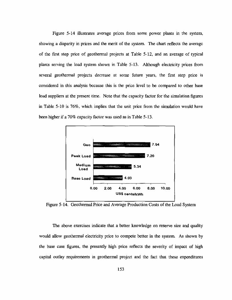
Figure 5-14 illustrates average pnces from some power plants in the system,
showing a disparity in prices and the merit of the system. The chart reflects the average
of the ftrst step price of geothermal projects at Table 5-12, and an average of typical
plants serving the load system shown in Table 5-13. Although electricity prices from
several geothennal projects decrease at some future years, the ftrst step price is
considered in this analysis because this is the price level to be compared to other base
load suppliers at the present time. Note that the capacity factor for the simulation ftgures
in Table 5-10 is 76%, which implies that the unit price from the simulation would have
been higher if a 70% capacity factor was used as in Table 5-13.
Geo
Peak Load
MediumLoad
Base Load
0.00 2.00 4.00 6.00 8.00 10.00
US$ centS/kWh
Figure 5-14. Geothermal Price and Average Production Costs of the Load System
The above exercises indicate that a better knowledge on reserve size and quality
would allow geothennal electricity price to compete better in the system. As shown by
the base case ftgures, the presently high price reflects the severity of impact of high
capital outlay requirements in geothennal project and the fact that these expenditures
153

have to be committed upfront. The expenditure designated for development wells can be
thought of as a commitment to purchase a large portion of the eventual fuel supply at the
project start-up (US Embassy Jakarta, 2002). Simulation results in Table 5-9 implies that
a pre-commitment on output prices where reserve feasibility is still in question adds more
upward pressure to the output price, since these prices are set with a smaller reserve and
plant capacity in mind. Further, this setting may induce opportunism behavior that tends
to increase the upward pressure to the price.
Table 5-12. Geothermal Power Plant Development Project
Power Plant YearContracted TariffUS$ centslkWh
1 Bedu~l 7.152 Cibuni 6.903 Daraiat 6.95*4 Dieng 1-14 9.81
15-22 7.4123-30 6.21
5 Kamoiang 4,5 7.036 Karaha 1-4 1-14 8.46
15-22 6.5723-30 5.63
7 Patuha 1-4 1-14 7.2515-22 5.6323-30 4.82
8 Salak 4,5,6 1-14 8.4615-30 4.94
9 Sarolla 1-6 1-14 7.6015-22 5.752-30 5.21
10 Sibayak 7.111 Wayang Windu 1-14 8.39
15-22 6.5123-30 5.57
*Reduced to 4.2 cenls folJowlllg a renegollallon III Apnl 2000Source: US Embassy Jakarta, 2002; PLN; Ministry of Mines and Energy
154

Table 5-13. Production Cost (US$ centsfkWh)
Plant Type Fuel Total Production CostBase Load Medium Load Peak Load
Steam Coal 4.195Steam MFO 3.745Closed Cycle.9as Turbine Gas 4.303Closed Cycle Gas Turbine HSD 3.891Diesel HSD 5.436Diesel MFO 5.238
-2pen Cycle Gas Turbine Gas 7.234Ooen Cvcle Gas Turbine HSD 6.673-Hvdro 7.699Average 4.0335 5.337 7.202Note: CapacIty factor for base load IS 70%, medium load 50%, peak: load 30-40%Source: A1anal et aI., 2000.
5.4 EXERCISE SUMMARY
The Option Theory calls for infonnation on the volatility of the change in price or
value of the underlying asset. This requirement implies that the underlying asset shall be
actively traded, such that the market provides sufficient data on price changes allowing
the respective volatility to be measured. The existing Indonesian capital market does not
permit a direct implementation of Real Option Valuation to geothermal electricity
project, since there is no electricity- or extraction- project related products in the market.
Further, the electricity sector is regulated, such that prices are stable at a certain level for
a long time with infrequent adjustment. Therefore, the volatility measure of the
underlying asset is nearly zero.
Copeland and Antikarov (2001) propose to represent the underlying asset value
by a properly anticipated stream of cash flows of the respective project. The change in
project value is represented by the rate of return of the cash flows. The variations in the
155

rate of return are due to changes in parameter values affecting the cash flows, such as
natural conditions of the reserve, financial parameters and the price components. This
approach makes possible an application of real option valuation to non-tradable real
assets.
The project is modeled as compound options, namely exploration option and
development option. Exercising the development option is by undertaking exploration
activities, which means spending the exploration costs (representing the strike price of
the option) to obtain the second option, which is the development option. Similarly,
exercising the development option is by undertaking development activities, which
means spending the development cost (representing the strike price of the option) to
obtain a project that generates revenue over the rest of the project life. At every time
period, the management can choose to continue investing, or delay investment decision
(option to wait), or stop the project to respond to unfavorable conditions (option to
abandon).
The exercise in section 5.2 describes an implementation of Copeland and
Antikarov approach to value managerial options in a hypothetical 110 MW geothermal
electricity project at the Indonesian business setting. Table 5-14 summarizes the results
of the exercise. ROA takes into account flexibility in the project investment decision,
and reflects the worth of this added feature at the time of valuation period, which is at the
start of the project. The options to defer and abandon investment show that flexibility
value in this exercise is positive, increasing the value of a good state by 41 %. This
implies that the conventional NPV undervalues the project.
156

Table 5-14. Results Summary
Method Value---_.__...........•._- --_._--_..-.-.--"_.•.•.($ million) Relative
Conventional NPV:
• Expected Total Value of Project 3
• Value of Good State" 42 BaseProject with Flexibility: Additional Value at the Good State
1. Options to Defer and Abandon Investment 17 (+41%)2. (I) & Option to Expand; targeting the Base Load Prod Cost 19 (+45%)3. (1) & Option to Expand; using the ex-ante price set 81 (+193%).. . ..
Note: a good state refers to the condltlon when the reserve feasIbilIty and SIze are suffiCIent tosupport electricity production, such that the project earns revenue.
Section 5.3 examines the possibility of realizing that the reserve is better than
previously estimated, which may mean higher productivity of wells, or lower costs, or
larger capacity of the reserve, or a varying degree of their combinations. The analysis
considers the impact of having an expansion option, in addition to the circumstances
described in section 5.2. The example examines twice as large capacity than initially
estimated, and the results show that real options consideration improves project value by
45%. It also provides information to allow managers decide an output price that can
compete with other base load suppliers and yet relates to a profitable project.
Further, exercising the expansion option and applying the ex-ante price yields a
highly profitable business. However, the latter also means an excessive burden to the
state utility company. The range of feasible prices associated with these conditions
indicates that there is a room for an improvement in the distribution of profit. The
flexibility value is almost twice as much as the conventional value of the project.
157

The above exercises show that price determination following the conclusion of
exploration activities provides both the possibilities of securing a profitable business and
at the same time relates the project with a competitive price. This outcome is a
consequence of focusing on the impact of having new information on the reserve
characteristics as a result of completing exploration activities. Nevertheless, the model in
this chapter is bounded within the private developer's internal decision assessment
without recognizing the presence of other active participants. In other perspective, the
model implicitly assumes symmetric information and a simple opportunistic behavior of
the market participants. Therefore, it is important to note that the results from this
exercise are based on those assumptions. Removing these assumptions opens a new array
of possible difficulties related to incomplete and asymmetric information, as well as
opportunistic behavior of the market participants. Chapter 6 proposes an arrangement to
addresses this issue.
158

CHAPTER 6
POLICY IMPLICATION
As stated previously, the model in Chapter 5 concentrates on the consequences of
natural characteristics of geothermal resources to the project. This implies less emphasis
towards the behavior of the parties. While the importance of their roles is considered,
strategic interrelationships among them are not critically important. The implicit setting
of the model can be described as follows: (i) agents inside the firm and the states of
nature determine the project value, which belongs to group 2 of investment literature
categories following Brennan and Trigeorgis (2000), (ii) the third party, who is assumed
to be the government, plays a role as regulator that provides laws and order to govern the
business. In addition, the model also employs two implicit assumptions, which are: (iii)
complete and symmetric information, and (iv) simple self-interest behavior of the market
participants. The exercise results suggest that an ex-post price determination is Pareto
improving.
In contrast to the prevIous setting, this chapter assumes incomplete and
asymmetric information, as well as opportunistic behavior by market participants. Under
this condition, an ex-post price determination may not work. Incorporating these
assumptions implies that the boundary of the problem has moved outward, incorporating
several participants and the impacts of their interaction with each other. Although the
research does not cover the institutional arrangement analysis in a formal way, the
following assessment highlights important features of the setting and the need for
159

institutional changes are indicative. The first section of this chapter reviews some
literature to describe the relationship of the parties. The second section illustrates the
possible difficulties related to the ex-post price determination. The third section proposes
a two-phase price determination to attenuate the difficulties associated with opportunistic
behavior as well as incomplete and asymmetric information.
6.1 INTERRELATIONSHIP OF THE PARTffiS
For the purpose of simplicity,47 let us assume that the parties involved in this case
are: (i) the government, which represents the people of Indonesia as the legal owner of
geothermal resources in the country, and (ii) a private developer, who has special skills,
expertise and financial support to develop a geothermal prospect.
A geothermal development project can be seen as a delegation48 of task from the
government to a private developer. The task is to develop a geothermal prospect such
that it can generate electricity and transfer the electricity back to the government at a
price. The government then distributes the electricity to the public at another level of
price.
Following the terminology of the institutional economic literature, in this context
the government is the 'principal' and the private developer is the 'agent'. Laffont and
Martimort (2002) state that, ''the essential paradigm for the analysis of market behavior
by economists is one where economic agents pursue, at least to some extent, their private
47 In practice, the developer represents a consortium of companies, while project financing involves aconsortium of banks and other financial institutions.48 The motivation to delegate can be the possible benefit related to the division of tasks or the lack of timeor ability to perform the task (Laffont and Martimort, 2002)
160

interests," which in different literature this paradigm is referred to as opportunism or
strategic behavior. From the point of view of The Incentive Theory, the task delegation
has two basic characteristics, namely conflicting objectives and decentralized
information. In terms of a geothermal project, these two characteristics can be described
as follows:
(i) Conflicting objectives: the principal would like to be able to have a developed
geothermal resource and to provide low price electricity for the public, while the
agent would like to maximize profit.
(ii) Decentralized information: by doing the task, the agent may get access to
information that is not available to the principal. Such information may include
the exact opportunity cost of this task, the precise technology used, as well as the
match between agent's ability and the technology used. In addition,
accomplishing a geothermal project development task also make available very
specific and valuable information about the underground resource condition.
Even if there is a regulation stating that this data shall be provided to the
principal, the opportunism behavior paradigm stated above indicates that there
remains a possibility that not all findings are reported.
Laffont and Martimort (2002) suggest that the implication of these informational
problems in task delegation generally prevent society from achieving the first-best
allocation of resources that could be possible in a world where all information would be
common knowledge. This means that the condition of asymmetric information lead to
161

incentive compatible contract that involves a trade off between information rent and the
allocative efficiency. As they put it:
".. the information gap between the principal and the agent has some fundamentalimplications for the design of the bilateral contract they sign. In order to reach anefficient use of economic resources, this contract must elicit the agent's privateinformation. This can only be done by giving up some information rent to theprivately informed agent. Generally, this rent is costly to the principal." (note: theoriginal text do not include underlines)
Williamson (1985) refers to this cost as transaction cost, which is defined as ''the
cost of running the economic system." The Transaction Cost Theory recognizes that
there are three principal dimensions that distinguish transactions (or contractual
relations), which are asset specificity, uncertainty, and frequency. Asset specificity refers
to distinctive skills, unique choice of locations, or special purpose investment.
Uncertainty may arise due to acts of nature, lack of communication, or strategic behavior.
Frequency of transaction matters since repeated transaction provides experience, which is
information that can be used as a reference in making decisions.
With respect to the above transaction dimensions, a geothermal project is an
idiosyncratic or highly specific investment. The geothermal wells drilled for the project
are location-specific and have a specific purpose, i.e., to transport the heat of the earth to
the surface. Moreover, undertaking the task requires special skills. The source of
uncertainty in the project is due to the course of nature, which determines whether the
prospect contains sufficient quantity and quality of energy. The task assignment takes
place only once, which is at the start of the project.
Williamson (1985, 1986) stated that once such idiosyncratic transaction has
entered into a contract, there are strong incentives to see the contract through completion.
162

Further, the interests of the parties to sustaining the relation are especially great for
highly idiosyncratic transactions. This is because in highly specific investment the agent
is effectively 'locked into' the transaction because the asset is not suitable for other
purposes. The principal is also committed to the transaction because of the skill
requirement for undertaking the task mastered by the agent, as well as possible costs
associated with any delay of production should the contract is interrupted or terminated.
Another implication of asset specificity is a fundamental transformation of the market
once the contract is signed. An ex-ante competition to enter a contract for an
idiosyncratic investment is effectively transformed into one of bilateral supply. This is
because economic values would be sacrificed if the ongoing supply relation were to be
terminated, except when such investment is transferable to an alternative party at low
cost.
Williamson (1986) suggests that 'Trilateral Governance' is an efficient
governance structure for such transaction, which is where the principal and agent enter a
not-so-comprehensive contract that facilitates transaction and the contract also includes
third party assistance. The third party function is to incorporate flexibility and to fill the
gaps in the contract, such as to solve dispute and evaluate performance. Further, he also
suggests that idiosyncratic investment can benefit from adaptive-sequential-contract
since it can attenuate opportunism.
163

6.2 EX-POST PRICE DETERMINATION
The research findings at Chapter 5 are important information to be considered in
determining the output price. Since expansion option is known after the exploration
works have been concluded, this finding also suggests that it is worth to consider
deciding the output price after the exploration stage. A price determination after the
exploration phase can be referred to as 'the ex-post structure,' in contrast to the ex-ante
system that presently prevails.
Assuming symmetrical information and a simple self-interest seeking behavior49
by both parties, the ex-post structure offers a set of incentives to develop geothermal
resources. From the company's point of view, this structure provides information to
consider a lower feasible price than the level dictated by the ex-ante price. These lower
and yet feasible prices would improve the chance of the company to compete with the
other base load suppliers, and therefore, securing their positions in the merit order of load
dispatch.
The ex-post structure is also of interest to the utility company, since (i) having
geothermal power plants supply power at competitive prices would reduce the financial
burden that is presently imposed to the utility due to the 'must-run' policy, and (ii) having
geothermal plants in the system means a diversification of supply base that could increase
reliability of the system.
From the point of view of the government, the ex-post structure would be able to
serve as a self-generating motivation for geothermal development that would hopefully
49 Information is fully and candidly disclosed upon request, accurate state of the world declaration, andoath- and rule-bound actions (Williamson, 1985).
164

attract more parties to participate. In addition, development of geothermal resources
would help ease the pressure on domestic demand for energy.
The above results show that under the assumption of symmetrical information and
minimal opportunistic behavior, the ex-post structure is Pareto improving. This
improvement would also be socially desirable, especially for many regions where
geothermal potentials have been identified and plans to develop the resources have not
materialized due to the existing problems.
However, the two assumptions above imply that the results are applicable in a
simple world. When such assumptions are relaxed, then the ex-post arrangement has to
deal with consequences of asymmetric information and opportunistic behavior of the
parties. The possible problems from the private developers' point of view are, (i) lack of
interest from private developers, since exploration spending does not guarantee access to
the development and operational stages, and (ii) if private developers are willing to take
the risk, their opportunistic behavior may lure them to charge excessive prices for the
private information they have from investing in the field study. The reciprocal problems
from the point of view of the government and the electric utility company are, (i)
opportunistic behavior by the government to take over the project, as better information is
available without any investment or obligation from their side, and (ii) hesitation from the
government and the electric utility company due to uncertainty on the output price to be
charged. These difficulties show that the ex-post structure is likely to fail.
165
6.3 TWO-PHASE NEGOTIATION
Some scholars and practitioners have suggested the pnce negotiation after
exploration, such as Enerindomurni (1999) and Electroconsult (1996). Nevertheless, an
implementation of this setting is likely to be difficult since there would be large
expenditures for the exploration phase that require the company to look for commercial
financing. Without any agreement concerning prices that reflect the expected value of
the project, it would be difficult to finance the project with outside funding.
Partowidagdo (2000) suggests coupling the ex-post structure with an exploration
insurance that reimburses the developer should the exploration fail to produce electricity
at a competitive price, while the fund comes from taxing the existing geothennal fields or
collecting a depletion premium from oil and gas extraction. This scheme may induce
participation in geothermal development. But again, in a world with incomplete and
asymmetric infonnation as well as opportunistic behavior, the private information on the
cost size and structure to undertake the exploration are not observable and therefore, may
motivate opportunistic behavior to overcharge the cost. Another possible opportunistic
behavior is, depending on the magnitude of the insurance coverage, an understatement of
the resource quality and quantity to obtain short-tenn benefit from the reimbursement in
return to neglecting the project. The potential financial liability may hinder government
participation in this scheme.
Williamson (1986) suggested that an adaptive-sequential contract could attenuate
opportunism behavior of the parties involved in an idiosyncratic investment project. An
alternative to incorporate flexibility that also addressed the opportunity concerns is a two-
166

phased price negotiation arrangement, where the fIrst phase sets a boundary of acceptable
prices for the project prior to any engagement and the second phase determines a specifIc
output price based on the exploration results.
Nodes Cl and C8 at Figure 6-1 represent the negotiation series. In contrast to the
previous project structure at Figure 5-1, node C1 at the present structure determines the
range of acceptable prices based on the prices of electricity from other power plants
supplying the base load. This step would ensure that only viable projects would survive
as candidate suppliers to the base load electricity system. The fIrst phase curbs the
transaction from an excessive opportunism behavior by the private developer.
Figure 6-1. Project with Two-Phase Negotiation167

The specific output price is determined at the second negotiation, which takes
place after the exploration stage. At this position, exploration results provide information
on a possibility to expand the capacity size. As previously illustrated by Table 5-9, the
size of expansion may be significant. A negotiation table with this information is likely
to draw a very different picture than that of the pre-commitment case. Some exercises for
this situation indicate a considerably wide range of feasible price level, which suggest
that the company would be able to lower the proposed price by significant points and still
meet the capital requirements of the investment. Therefore, the second phase negotiation
would facilitate a more realistic project valuation for both parties at the negotiation table.
In this case, the first phase agreement serves as pre-commitment conditions for
both parties. It says that only viable projects would survive as candidate suppliers to the
base load electricity system, addressing the possible opportunism behavior by the private
developer. On the other hand it also says that the price range indicates acceptable
charges, therefore it can be seen as a purchase guarantee from the government.
Conducting the second phase negotiation after the completion of exploration activities
would provide better knowledge on reserve characteristics and feasibility, and would
facilitate a more realistic project valuation for both parties at the negotiation table.
6.4 CONCLUDING REMARKS
This research focuses on the influence of natural characteristics of geothermal
reserves to the project value, and concluded that there are benefits from recognizing
managerial flexibility into project valuation. This information can be used to facilitate
168

the transaction process between the government and potential private developers of
geothennal projects. To be able to focus on the natural characteristics of the reserve, this
research incorporates several simplifying assumptions such as isolating the project from
the rest of the economy and a minimal level of opportunism behavior by the market
participants. Some possibilities for future research agenda that build upon the present
results are to proceed in the following directions:
(i) Principal-Agent relationship:
Utilize the game theory or game theoretic approach to institutional analysis in
analyzing strategic behavior of the market participants and the respective
contractual ramifications. One possible area is the safeguard against opportunism
behavior by both the government and the private developer with respect to the
two-phased negotiation. Another area is to figure out the incentive compatibility
structure of the project.
(ii) Different settings:
Analyze geothermal projects that separate field development from power
generation activities. This structure involves at least two different transfer prices.
(iii) Assumption:
Testing the assumption that 'appropriate' projection of cash flow is an unbiased
estimate of the asset value. Develop criterion for detennining whether or not a
cash flow projection is appropriate, what are the important factors that need to be
considered.
169

APPENDIX A
MODELS FOR INVESTMENT VALUATION:
STRENGTHS AND WEAKNESSES
The following evaluation is a summary of Lander (1997) and Lander and Pinches
(1998) works.
A.I. Option-Based Models
Strengths:
• They are based on theory and, at least conceptually, can be used to model and value
many types of business decisions,
• Flexible, can be simple yet powerful decision-making framework
• Use risk-free rate and risk-neutral probabilities, therefore avoids the issue of risky
discount rates and risk preferences,
• Eliminates the need to estimate the expected rate of change in the underlying asset,
• Introduces asymmetry into the distribution of investment opportunity values,
• They model risk directly (a), in contrast to the DCF that represent it in the risky
discount rate,
• Highly appropriate when the volatility of the underlying asset is high, and there are
sequential or phased projects
170

• Powerful and robust when traded securities are available for parameter estimation,
since future values and cash flows are market determined (not based on projected or
estimated cash flows) and the need for subjective probabilities are avoided.
Weaknesses:
• Assume the decision to exercise is clear-cut,
• Limited by the difficulties in determining and modeling the state variable(s),
• Theoretically require complete markets and no arbitrage opportunities assumptions to
hold,
• Can quickly become complex and computationally demanding
• May provide a valuation and an initial optimal strategy, but do not necessarily
provide guidelines for managing the investment opportunity,
• Severely limited if there are more than one or two fundamental sources of uncertainty
A.2. Decision Tree
Lander and Pinches (1998) note that "most of the theoretical work in real options
indicates that decision trees are the least preferred decision-making frameworks" for
modeling and valuing real option. However, they disagree with this view and argue that
decision tree models and binomial models are equivalent when they are given the same or
corresponding data. Their arguments are:
• Traditional decision trees use subjective probabilities as well as a risky discount rate
that represent both time and risk preferences. However, this is similar to the discrete-
171

time option-based models, although in the latter the probabilities are transformed into
pseudo-probabilities in order to allow the use of risk-free rate as the discount rate.
• When the analysis is based on cash flow estimates (that is, if market information is
not available), a decision tree model has the same data demands as an option-based
model.
Nevertheless, there are major weaknesses of the traditional decision tree:
(i) The arbitrariness of the discount rate to value the tree indicates that decision trees
do not properly model the volatility when an option is present (similar concern as
in the traditional DCF model). The discount rate for the underlying asset alone is
not the same as the discount rate for a tree as a whole (because the tree contains
option). Lander and Pinches (1998) states that there is no direct way of
determining the appropriate! discount rate for the tree.
(ii) The problem with the size and complexity of the decision tree (this is actually also
present in the binomial and lattice models). It needs knowledge on joint
probability distribution, and significant effort to preprocess the probabilities in a
relatively complex problem. Modeling more options would result in
exponentially larger size of the tree, however often not substantial in determining
additional value.
(iii) Estimating the probabilities of the future uncertain values or cash flows.
However, note that this is also the weakness of a traditional DCF and may be an
option-based model when market price of the underlying variable is not available.
1 This refers to the 'corresponding' discount rate that would make the analysis equivalent to that of anoption-based model.
172
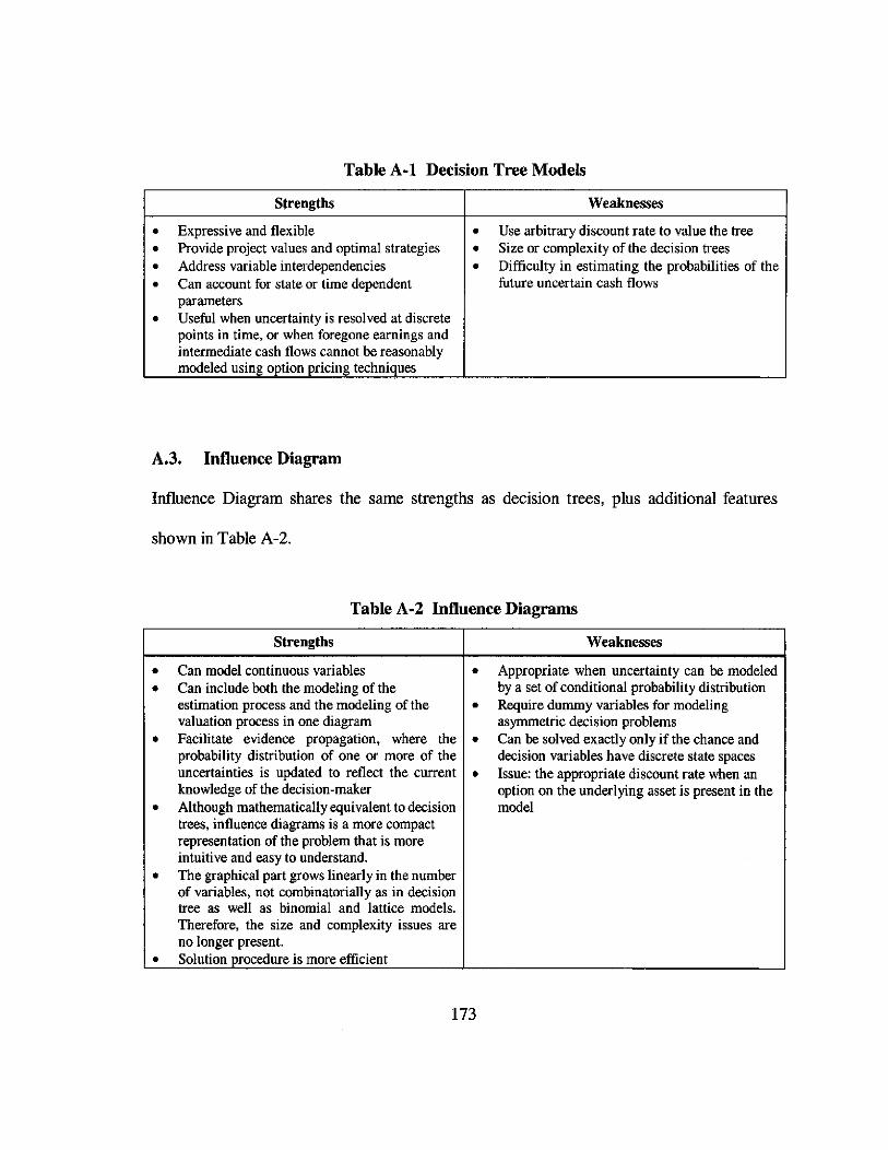
Table A-I Decision Tree Models
Strengths Weaknesses
0 Expressive and flexible 0 Use arbitrary discount rate to value the tree0 Provide project values and optimal strategies 0 Size or complexity of the decision trees0 Address variable interdependencies 0 Difficulty in estimating the probabilities of the0 Can account for state or time dependent future uncertain cash flows
parameters0 Useful when uncertainty is resolved at discrete
points in time, or when foregone earnings andintermediate cash flows cannot be reasonablymodeled using option pricing techniques
A.3. Influence Diagram
Influence Diagram shares the same strengths as decision trees, plus additional features
shown in Table A-2.
Table A-2 Influence Diagrams
Strengths Weaknesses
0 Can model continuous variables 0 Appropriate when uncertainty can be modeled0 Can include both the modeling of the by a set of conditional probability distribution
estimation process and the modeling of the 0 Require dummy variables for modelingvaluation process in one diagram asynnnetric decision problems
0 Facilitate evidence propagation, where the 0 Can be solved exactly only if the chance andprobability distribution of one or more of the decision variables have discrete state spacesuncertainties is updated to reflect the current 0 Issue: the appropriate discount rate when anknowledge of the decision-maker option on the underlying asset is present in the
0 Although mathematically equivalent to decision modeltrees, influence diagrams is a more compactrepresentation of the problem that is moreintuitive and easy to understand.
0 The graphical part grows linearly in the numberof variables, not combinatorially as in decisiontree as well as binomial and lattice models.Therefore, the size and complexity issues areno longer present.
0 Solution procedore is more efficient
173

APPENDIX BGEOTHERMAL DEVELOPMENT ININDONESU
0' N
+10"5
o <;00 400 600 000I
Ki_
South ChinaSea
~
11~E
"
INDONESIAN OCEAN
INDONESIAlldE
12soe
12S"E
Philippine Sea
-II,.
PACIFICOCEAN
IfArafura sea
5' N
~
lds
Source: Sub Directorate of Geothermal Survey, Directorate General of Geology and Mineral Resources, Miuistry of Mines and Energy of Indonesia, 1998.
Figure B-1. Geothermal Prospects in Indonesia
174

Notes for Figure B-1. Geothermal Prospects in Indonesia (1998)
ACEH 45. Bukit Kili 86. Gunung KarangI. Lho Pria Laot 46. Surian 87. Pulosari2. Kaneke 47. Gunung Talang 88. Cianten - G. Bndut3. Iboih-Jaboi 48. Muaralaboh 89. Pamancalan4. Le Suum Krueng Raya 49. Liki Pinangawan 90. KawahRatu5. Seulawah Agam RIAU (G. Salak)6. A1ur Canang 50. Pasir Pangaravan 91. Kawah Kiara Beres7. A1ue Long-Bangga JAMBI (G. Salak)8. Langsa 51. Gunung Kapur 92. AwiBengkok9. RimbaRaya 52. Gunung Kaca (G. Salak)10. G. Geureudong 53. Sungai Tutung 93. Ciseeng11. Simpang Balik 54. Semurup 94. Bujal- Jasinga12. SHih Nara 55. Lempur 95. Cisukararne13. Meranti 56. Air Dikit 96. Selabintana14. Brawang Buaya 57. Graho Nyabu 97. Cisolok15. Kafi 58. Sungai Tenam! 98. Gunung Pancar16. Gunung Kembar BENGKULU 99. Jarnpang17. Dolok Perkiraoan 59. Tambaog Sawah 100. Tanggeung-NORTH SUMATERA 60. Bk. Gedang-Hulu Lais Cibungur18. Beras Tepu 61. Suban Gergok 101. Saguling19. Lau Debuk-debuk Sibayak 62. Lebong Simpang-Bukit Daun 102. Cilayu20. Marike 63. Taniun" Sakti 103. Kawah Cibuni21. Dolok Marawa SOUTHSUMATERA 104. G. Patuha22. Pusuk Bukit 64. Sungai Liat 105. Kawah Ciwidey23. Simbolon-Samosir 65.PangkalPinang 106. Maribaya24. Pagaran 66. Air Ternbaga 107. G. Tangkuhan25. Helatoba 67. Rantau-Dadap-Segamit Parahu26. Sipaholon-Ria-ria 68. Bukit Lumut Badai 108. Sagalaherang27. Sarula 69. Ulu Danau 109. Ciarinem28. SibuaJ-buali 70. Marga Bayur 110. G. Papandayan29. Namora \langit 71. Wai Selabung Ill. G. Guntur - Masigit30. Sibubuhan LAMPUNG 112. Kamojang31. Sorik Merapi 72. Wai Umpu 113. Darajat32. Sampuraga 73. Danau Ranau 114. G. Tampomas33. Roburan 74. Purunan 115. CipacingWEST SUMATERA 75. Welirang Sekincau 1I6. G. Wayang Windu34. Simisioh 76. Becingot 1I7. G. Talaga Bodas35. Cubadak 77. Suoh Antatai 1I8. G. Galunggung36. Talu 78. Pajarbulan II9. Ciheras37. Panti 79. Natar 120. Cigunung38. Lubuk-Sikaping 80. Ulubelu 121. Cibalong39. Situjuh 81. Lernpasing 122. G. Karaha40. Bonjol 82. Wai Ratai 123. G. Sawal41. Kotabaru-Marapi 83. Kalianda 124. Cipanas - Ciawi42. Maninjau 84. Pematang Belirang 125. G. Cakrabuana43. Sumani WEST JAVA 126. G. Kromong44. Prian"an 85. Rawa Dano 127. SangkanuriD
175

Notes for Figure B-l. Geothermal Prospects in Indonesia (1998) (continued)
128. Subang 166. Wai Pesi 207. Sulili129. Cibinbin 167. Inelika 208. MalawaCENTRAL JAVA 168. Mengaruda 209. Baru130. Banyugaram 169. Bobo 210. Watampone131. Bumiayu 170. Komandaru 211. Todong132. Baturaden 171. Ndatusoko 212. Sinjai133. Gud 172.Sokoria 213. Masepe134. Mangunan - Wanayasa 173. Jopu 214. Danau Tempe135. Candradimuka 174. Lesugolo SOUTHEAST136. Dieng 175.0ka SULAWESI137. Krakal 176. Atedai 215. Mangulo138. Panulisan 177. Kalabahi 216. Parora139. Gunung Ungaran NORTH SULAWESI 217. Puriala140. Candi Umbul 178. Air Madidi 218. Amohola141. Kuwuk 179. Lahendong 219. Loanti142. Gunung Lawu 180. Tompaso 220. Laenia143. Klepu 181. Gunung Ambang 221. TorahYOGYAKARTA 182. Kotamobagu 222. Kalende144. Parangtritis 183. Gorontalo 223. KanaleEAST JAVA 184. Petandio 224. Wonco145. Melati CENTRAL SULAWESI 225. Rongi146. Rejosari 185. Maranda 226. Kabungka147. Telaga Ngebel 186. Sapo 227. Sampulawa148. G. Pandan 187. Langkapa MALUKU149. G. Arjuno Welirang 188. Napu 228. Mamuya150. Cangar 189. Torire 229. Ibu151. Songgoriti 190. Toare 230. Akelamo152. Tirtosari 191. Patalogumba 231. Jailolo153. Argopuro 192. Merawa 232. Kie Besi154. Tiris 193. Bora 233. Akesahu - Tidore155. Blawan lien 194. Pulu 234. IndariBALI 195. Sedoa 235. Labuha156. Banyuwedang 196. Wuasa 236. Tonga157. Seririt 197. Watuneso 237. Larike158. Batukao 198. Papanpulu 238. Taweri159. Penebel SOUTH SULAWESI 239. Tolehu160. Buyan - Bratan 199. Luwuk 240.0ma-HarukuWEST NUSA TENGGARA 200. Parara 241. Saparua161. Sembalun 201. Pambusuan 242. Nusa Laut162. Marongge 202. Somba IRIAN JAVA163. Huu Daha 203. Mamasa 243. Makbau-SorongEAST NUSA TENGGARA 204. Bituang-Rantepao 244. Ramsiki-Umsini164. Wai Sano 205. Sangala-Makale165. Ulumbu 206. Senjl;kanjl;
176

Table B-1. ACTIVITIES IN GEOTHERMAL PROJECT DEVELOPMENT
Activities Objective & Description of Activities Time Notes
1. EXPLORATION To proof the existence of the resource & assess the resource ± 4 years Cost estimate US$ 20-30 Millionpotential
1.1 Reconnaissance Survey • Identify surface manifestation that indicates possible ± 1 year • Cost estimate: US$ 0.1-0.3
(Preliminary Exploration) existence of geothermal resources Million
• Produce documentation on regional geology of the site • Approximate degree of
• IdentiI)' possjble uti Iization of the potential resource & success thal the prospectprellmjnary market study could be commercially
developed: 30%-50%
a. Literature Study • Collect maps and data from previous survey activities in the 1 month Time requirement depends onarea data availability & accessibility
• Determine locations to be surveyed
b. Field Survey: • Identify global formation and types of earth's crust, rock 3 month- Time depends on the quality of
• Geological configuration, geological structure, surface manUestations 1 year existing data; area to be covered
• Hydrology and their respective characteristics (range varies from a few to
Geochemistry • Take fluid samples, measure the temperature, pH and now thousands km!), geological• rate conditions; and team size• Environment Identify environmental constraints•
c. Data Analysis & To obtcin geological and hydrological model of the area:
Interpretation • To determine the prospect area (conclude the boundaries)
• To estimate the type of reservoir, it's temperature, waterori~in and type of rock that form the reservoir
d. Speculate on the However limited, the data shaH be used to estimate electricity Indonesia: 20 km2 == 2.5 MWeelectricity potential potential of the resource. Statistical figures of the existing
geothermal projects are commonly used as benchmark.
e. Preliminary market To verify the existence of power demand that could be fulfilled
study by the generation from the potential geothermal resource
f. Propose future activities • Decide whether to continue the project or to abandon it.
• If decided (Q continue, then recommend priority locationsfor further investigation and the respective survey type tobe conducted on the next phase of the proiect
177

Table B-1. ACTIVITIES IN GEOTHERMAL PROJECT DEVELOPMENT (continued)
Activities Objective & Description of Activities Time Notes
1.2 Pre.Feasibility Study • Enhance the knowledge on the prospects by stndying I year • Cost estimate:
(Advance Exploration) indirect evidence of the conditions that affects the existence US$ 0.5-2 Millionof a geothermal reservoir • If the investigation result is
• Delintitate the area of probable occurrence of the reservoir positive, there is 50%
• Lead to a decision whether or not to continue with probability of eventuallyexoloration activities discover a commercial field
3.. Field Survey:• Advance Geology • Obtain detail geology and stratigraphy information of the
• Advance Geochemistry site
• Take samples from all locations of surface manifestationand the surrounding area to examine fluids and gas at thesurface as well as underneath (inspect for corrosiveness and
• Hydrology other potential problems)
• Advance Geophysics • Study the groundwater circulation system
• Geography • Delineate the possible position of the reservoir
• Obtain information on the contour of the area, the existinginfrastructure (road, clean water, electricity,
• Drilling of slim holes telecommunication), and the surrounding population
• If surface investigation leaves some doubt on the existenceof an active heat source, slim exploratory wells may bedrilled to test the temperature at 500-800 m depth
b. Data Analysis & To produce a prelintinary geothermal model of up to 1-4 km
Interpretation below surface, which enable the estimation of resourcepotential, recoverable reserve, and electricitv ootential
c. Propose future activities • Decide whether to continue the project or to abandon it.
• If the project is considered to be likely econonticallyfeasible, then identify target and location ofexplorationdrilling as well as the resnective drilling program
178

Table B-1. ACTIVITIES IN GEOTHERMAL PROJECT DEVELOPMENT (continued)
Activities Objective & Description of Activities Time Notes
1.3 Feasibility Study 0 To proof the existence of geothermal resource in the area ±2 years 0 Cost estimate: US$ 10
(Detail Exploration) 0 Decide whether the prospect is technically and Millioneconomically feasible, hence attractive for development. 0 70% success ratio to lead to
nroven commercial fields
a. Reservoir & Steam 0 To evaluate field characteristics (quality, quantity, depth) Exploration well generally costs
Production Engineering: and estimate its potential (proven, probable, possible)*: more than production well since
0 Drill exploratory wells - Commonly drill 3-5 deep exploratory wells (1000-3000 it involves:
Data analysis & m) to have 2-3 producing wells and at least I re- o More careful approach due0
interpretation injection well to the uncertainties involved
Evaluate geothermal model - Obtain information on the type and characteristics of 0 Drilling of deeper holes for0
reservoir (fluid; depth, type, temperature, rock) reservoir investigation0 Decide whether there is enough information to assess the 0 More measurements to
resource potential. or more exploration wells need to be better understand thedrilled. Ifsome exploration wells show enough potential, underground situation andthen continue with examining the feasibility for reservoir characteristicsdevelopment Cost estimate (Indonesia):
0 Test and adjust the geothermal system model previously US$ 2.1 Million/exploratorydeveloned well
b. Power Plant Engineering Aimed at the optimization of the conversion process of thegeothermal resources into electricity:
• Select conversion process, development strategy, unit size0 Select plant site and determine general design0 Identify acceptable measures to mitigate environmental
imoacr
c. Economic Evaluation 0 Pre-requisite: completion of J.3-a and 1.3-b that yieldproven reserve
0 Demand assessment0 Compare the cost of implementing the project to the
exnected benefit from the sale of generated energy
d. Propose future activities Decide whether the prospect is technically and economicallyfeasible, hence attractive for development. If yes, then continuewith detail planning for nroject imolementation
179

Table B-lo ACTIVITIES IN GEOTHERMAL PROJECT DEVELOPMENT (continued)
NotesObjective & Description of Activities
Produce steam from production wellsGenerate electricity at the power plant
Obtain necessary information to decide whether to plan thedrilling of replacement wells or an expansion of productioncapacity through:• Constantly monitor reservoir performance to detect
significant variation that may indicate the decline ofproduction
• Constantly calibrate the mathematical model of thereservoir
Drill make-up wells to compensate the depletion of the'roduction wells due to the draw-down of the reservoir
To determine necessary systems and facilities to be in place,which includes detail engineering design and other aspects offield development as well as power plant construction:
Monitoring
b. Power PlantConstruction
Planning
Maintenance
A critical phase in a geothermal==9 project
Cost estimate: US$1200 - 2200per kW installed (depends on
2.2 IProject Implementation power plant size, wellsa. Drill Production & • Drill sufficient production wells to ensure enough steam productivities and costs)
Injection Wells • Drill injection wells, that are used to return the waste water Average development well in!ilto the ground Indonesia
• Update reservoir assessment • Success ratio: 80%• Develop the power plant and the respective infrastructure 24-30 • Cost: US$ 1.5 Million/well
(critical activity: the supply & erection of the turbine and months • Productivity: 7 Mwe/wellgenerator) (World average: 5 MWe)
3.3
2.1
3.2
Notes: 'Proven reserve: the highest degree of resource potential estimation that is based on information from at least one exploratory well and two delineatedwells; Probable: less certain than 'Proven', based on information from an exploratory well~ Possible: the least certain estimation, information is based ongeological, geochemistry and geophysics surveys.Source: Directorate General of Electricity and Energy Development of Indonesia, 1995, "Private Power Development: Geothermal and Combined Cycle Projects,Geothermal Total Projects, Volume III", Study Report by Electroconsult, Fichtner and Redecon.
180

Table B-2. COSTS OF A GEOTHERMAL PROJECT
) Wells for a 55 MW eotnermal oower lant are assumea as TallOWSProducers Reiniectors Failed Total
Exploration 2 1 2 5Development 8 1 1 10Reiniection (add'i) - 2 1 3
Notes.." Average Indonesian data from the existing commercial fields
...... Geothermal field in Indonesia is commonly water dominated.Hence, the stated cost estimate is for the 8 water-dominated producing wells (reter to the table below)
...... Statistics: average productivity of Indonesian wells is around 7 MWelwellAssumptions:
(a
Project stages # of well (al Cost/well"" Well Cost Other Cost Total Cost CostlkWUS$ US$ US$ US$ % US$/1<W
Exploration 10,350,000 1,850,000 12,200,000 6.1 221.82Reconnaisance 100,000Pre.f"easibility 1.000.000Feasibilitv 5 2,070,000 10,350,000 750,000
Development 25,660,000 52,766,000 78,426,000 39.1 1,425.93Field development 13 1,500,000 19,500,000Separation & gathering system1t* 8 770,000 6,180,000Power Plant (55 MWY" 50,000,000Other costs:
Access Roads & Land Rights 200,000Enaineerina & Administration{bj 2,566,000
Operation & Maintenance 46,130,000 63,935,800 110,065,800 54.8 2,001.20Syslem O&M (oj 27,380,000Make-up wells 1 every 2 yrs 1,500,000 18,750,000
Engineering & administration (d) 1,435,800Power plant operation 62,500,000
Total Cost lor a 55 MW Installed Capacity (US$): 82,140,000 118,551,800 200,691,800
Total Cost lor a 55 MW Installed Capacity (US$I1<W): 1,493.45 2,155.49 3,648.94"'_~
(b) Lifetime of Ihe project is 25 yearsEngineering & administration cost is estimated at 10% of total invesbnent costs
(c) System O&M per year is estimated a12% of the total well investment costs(d) About 10% of the yearly expenditures
Sources: Eiectroconsuil Report for DGEED, 1996; PT Bayu Enerindomumi Report for DGOG, 1999
181

APPENDIXC
INFLUENCE DIAGRAMS
Influence Diagrams (ID) are commonly grouped as one of the methodologies in
Decision Analysis. However, some similar features of other methodologies may lead to
inconsistent classification in the literature. Section C.1 briefly reviews the relationship
between ID and other graphical modeling that uses Bayesian approach.
Section C.2 sketches the intentions underlying ID conception and summarizes the
framework. Section C.3 introduces a formal representation of basic features of ill.
Section C.4 elaborates some issues related to the elements and structure in an ill
representation. Section C.5 describes appropriate structure of an ill, the two evaluation
procedures and their respective algorithms. Section C.6 briefly looks at a few
commercially available computer software to model and analyze ill. Section C.7
describes the components of the Base Case model of this research stated in Chapter 5.
Section C.8 provides additional notes for the proposed arrangement to improve some
problems in the Base Case model.
C.I The Family of Decision Analysis
Howard and Matheson (1989) describe Decision Analysis (DA) as a "discipline
comprising the philosophy, theory, methodology, and professional practice necessary to
formalizes the analysis of important decision". Decision Trees, Influence Diagram, and
182

Valuation Network are among the methodologies in DA that can be used to formally
represent a decision problem.
DA deals with issues of knowledge acquisition, knowledge representation, and
inference l. However, these issues are also shared by another strand of discipline called
Artificial Intelligence (AI). Abramson (1993) observes that the two disciplines can be
distinguished by their psychological motivations. DA is a sophisticated outgrowth of
task analyses of inference, evaluations and decisions; while AI is rooted in descriptive
psychology or observation about the way people behave. Consequently, DA prescribes
what decision makers should do, while an ideal rule-based AI would mimic the behavior
of a human expert. He also notes that both DA and AI could be considered as members
of a large family of models called Belief Networks, which is a graphical embodiment of
hierarchical Bayesian analysis.
Bayesian approach presumes that there are certain states of the world, one of
which includes the particular situation being examined (Morgan, 1968). The analyst
would deal with uncertainty by assigning probabilities to the possible states of the world.
Hence, such probabilities are often referred to as "personal or subjective probabilities"
and it is reasonable to ask an expert for an opinion about a rare event. In Bayesian
statistics probabilities are seen as orderly opinions, in contrast to those in Classical
statistics where they are frequencies of occurrence that consequently requires voluminous
data to obtain the information.
I Inference is the process of generating new conclusions from existing knowledge (Gottinger et ai, 1995).
183
The family of Belief Networks consists of directed-acyclic-graphicaI2 (DAG)
representation of a problem that have the following characteristics:
(i) Nodes represent individual variables, items, characteristics, or knowledge-
sources,
(ii) Arcs demonstrate influence among the nodes,
(iii) Functions associated with the arcs indicate the nature of that influence.
Prior to 1980, the only known member of the family of Belief Networks is
Decision Tree. More recently developed methodologies are Influence Diagrams (ID) in
the DA group and Bayes Network in the AI group. Over time, the advancement of these
methodologies leads to many shared characteristics. Ongoing improvements in the
weaknesses of each methodology have partly benefited from leading features of each
other in the form of hybrid methods. This progress yields more versatile approaches and
may have more efficient computational storage or time, but also lead to vague
classification.
For example, Ezawa (1998) refers to ill as a generalized Bayesian Network.
Sometimes it is not clear which is the general model and which is the special case.
Ndilikilikesha (1993) states that an ID containing only nodes representing the random
variables is called a Belief Network, while Varis (1997) states that ill is often considered
as a special case of Belief Networks.
Within the works that based on ID, there are many variants that correspond to
proposed modifications or advancement by various authors. Bielza and Shenoy (1999)
2 Directed graph with no loops. Directed graph means the arcs connecting the nodes are arrows thatindicate the direction of inflnence (either causal or relevance) among the nodes.
184

feel the need to put a reference for these ID variations, such as "Smith-Holtzman
Matheson's Influence Diagrams" and ''Tatman-Shachter's extension of the Influence
Diagram". Significant amount of works combine ID and Decision Tree (DT) in varying
ways, where the ID is used to represent the uncertainty of information and the DT is used
to represent the structural asymmetry information.
Some other works claim that they develop a new methodology, but later authors
consolidate these leading features back into ID framework. For example, although
Valuation Networks are similar to ID in many ways, they do not require conditional
probability and introduce solution technique called 'fusion algorithm'. However, as
stated by Shenoy (2000), further development by Ndilikilikesha (1992, 1994) has
translated the fusion algorithm into the ID framework.
Another strain of work combines DA with advances m related computational
mathematics of AI. For example, GOllinger and Weimann (1995) integrate artificial
intelligence-based techniques, logic-based approaches of problem solving with
techniques for probabilistic analysis and decision-making under uncertainty from
operations research and management science. Bielza et al (2000) show the need to
incorporate various techniques including those used in Bayesian Network for solving
complex decision-making problems with ID.
C.2 Influence Diagrams Framework
Influence Diagrams (IDs) were originally conceived to function both as a
computer-aided modeling tool and as a representation of the decision problem that is
185

easily understood by 'people in all walks of life and degrees of technical proficiency'
(Howard and Matheson, 1981). IDs would allow many of the decision analysts' tasks to
be implemented by personal computers such that the analysts can concentrate on major
Issues. IDs would also allow better communication between decision makers and
decision analyst experts.
An Influence Diagram (ID) is a network representation for modeling uncertain
variables and decisions. The graph shows the structure of the model, which consists of a
node for each variable in the model and arcs that indicate the relationships among the
variables. The nodes can represent constants, uncertain quantities, decisions, or
objectives. The arcs denote the probabilistic dependence of the uncertain quantities and
the information available at the time of the decision. Each node contains detailed
information about the respective variable (Shachter, 1986 & 1988).
An ill is not a flowchart, although it may look like one. Instead, as Clemen
(1995) states, it is a snapshot of decision maker's understanding of the decision situation
at a particular time. Hence, all decision elements that play a part in the immediate
decision need to be taken into account. Uncertain events are modeled using probability,
which indicate that the decision maker has some idea of how likely the different possible
outcomes are.
There are three levels of specification in an ill, (i) relation, (ii) function, and (iii)
number. Howard and Matheson (1981) and Smith et al (1993) explain this arrangement
as follows:
186

• In the deterministic case, the level of relation indicates that one variable depends in a
general way on others; for example, profit is a function of revenue and cost. The
level of function specifies the precise function describing this dependence; such as
profit equals revenue minus cost. At the level of number, numerical values of
revenue and cost are specified, and consequently this determines the numerical value
of profit.
• In the probabilistic case, the level of relation indicates that, given the information
available, one variable is probabilistically dependent on certain variables and
probabilistically independent of others. For example, we might assert that for a given
person, income depends on age and education, and that education depends on age.
The level of function describes the form of these dependencies, such as, if we divide
age into lO-year increments, we might assign different distributions on education for
each age group under 40 and the same distribution for all age groups over 40. When
assessing income given age and a particular educational level, we may wish to assign
distributions for each age group. At the level of number, we specify numerical
probabilities for each conditional and unconditional event. Taken together, the three
levels implicitly determine a joint probability distribution over all variables.
Once the decision problem is identified, the ID representation can be evaluated
using either one of the following ways. The first evaluation procedures analyzes the
diagram directly through a series of transformations that preserves the solution value,
although the graphical structure and the detailed data within the nodes are changed.
Shachter (1986) called such transformation as a value-preserving reduction, which may
187
be accomplished through (i) node removal, and (ii) arc reversal. The nodes that do not
influence other nodes or do not affect the objective can be automatically removed, while
the removal of other nodes are governed either by conditional expectation or conditional
optimality principle. Shachter (1988) notes that this is just the basic steps in evaluating a
stochastic dynamic program introduced in Bellman (1957). The arc reversal is the
implementation of Bayes' Theorem. Further elaboration on these solution procedures is
covered in Section D.4 of this appendix.
The second approach converts the ID into a corresponding DT representation, and
then solves the decision problem in DT form by following the rollback algorithm.
Marshall and Oliver (1995) note that the rollback algorithm was introduced by Raiffa
(1968), but it is actually based on the principle of optimality in dynamic programming by
Bellman and Dreyfus (1962).
C.3 A Formal Representation
The description of influence diagram in this section is a summary of related
materials in Howard and Matheson (1981), Shachter (1986), Ndilikilikesha (1994) and
Fagiuoli and Zaffalon (1998).
Let G = (N, A) be a directed-acyclic-graph (DAG),
where N = set of nodes
A = set of arcs, A (;; N x N
188

For any node tEN, define:
n(t) == ~E N!(S,t)E A}
cr(t) ==~E NI(t,S)E A}
n(t) == the set of direct predecessors of t
cr(t) == the set of direct successors of t
A node t is called a source if n(t) == 0, or a barren if cr(t) ==0.
For any set W ~ N , let n(W) == Un(t) and ~ (W) == W Un(W)..,eW
The nodes are partitioned into three sets: N == CUD U{v}. The nodes in C are called
chance nodes, the nodes in D decision nodes, and v is called value node or result node.
The arcs entering a chance or value node are called conditioning arcs; the arcs
entering a decision node are said informative arcs3• The informative arcs represent a
basic cause/effect ordering, while the conditioning arcs represent a somewhat arbitrary
order that may not correspond to any cause/effect notion and that may be changed by
application of the laws of probability such as Bayes' Rule.
Any node tENis associated to a variable X,E Q" where IQ,I(oo ; a generic
value of X, is denoted by x,. If W is a generic non-empty set of nodes, Xw denotes the
vector of variables indexed by the elements of W and with values in Q, == x leW Q, . If t
is a decision node, Q, is the set of the decisions associated with t. If t is a chance node,
the values in Q, are the possible states of the random variable X,; and for any value of
X.(I) it is defined the conditional probability distribution p[x, IXnuJ3 At least Howard and Matheson (1981) as well as Fagiuoli and Zaffalon (1998) use these terminologies.Howard (1990) uses 'relevance' to describe an arrow between chance nodes or between a chance node anda deterministic node, and 'influence' to describe an arrow from a decision node to a chance node.
189

The case of value node is slightly different. The node v must express the utility
value that is the consequence of a certain state of v parents, and therefore should contain
a function u: QO(') --7 Q,. The same concept is expressed in a different way by
considering X, a random variable and realizing the function u by means of the
probability:
if
otherwise
(D.I)
In fact, u(XO(,J = Lx,Plx,IXo(,J Using probability (D.I) has the advantage ofx,
treating the result node as a random variable.
Definition 1. An Influence Diagram is a pair (G,P) such that:
1. G = (N, A) is a DAG such that N =CUD U{v} and the following conditions are
satisfied:
(i) v is barren
(ii) there exists a directed path connecting all the decision nodes and only
them (single decision-maker property)4
(iii) the direct predecessors of any decision node are direct predecessors of all
the subsequent decision nodes (no-forgetting property)
4 This implies a lotal ordering among decision nodes (Howard and Matheson, 1981).
190

2. P is the family of conditional distributions associated to the nodes in C U{v}.
Defmition 2. Let G =(G, P) be an ID and t a decision node.
A function dt : QK(.) ...... Q t is called a decision function of t.
Note that the nodes in D model the decisions by means of decision functions. As in the
case of the result node, the decision function of t can be expressed in an equivalent way
by means of the following probability:
if
otherwise
(D.2)
Definition 3. A strategy for an influence diagram is the function s: QK(D)ID ...... Q D
resulting by the application of all the decision functions. A partial strategy SK is a
strategy related to a subset K of decision nodes.
When a strategy is fixed, probability (D.2) makes it possible to associate a set of
conditional probabilities to the decision nodes and hence to fonnally treat the decision
nodes too as chance nodes5• In this case any node of the graph is fonnally a chance node.
Fagiuoli et al (1998) show that ID is equivalent to Bayesian Network in many
ways. These features allows the factorization theorem to be extended to IDs,
5 Smith et a1 (1993) refers to this feature as 'determining a decision node'. See also section D.3.
191

P, [xN]= ITplx,IX.(t) J IT P, lx,IXnv)J~CU~} ~D
(D.3)
Expression (D.3) shows that the joint distribution is the product of the conditional
distributions of the nodes. The subscription s indicates that a strategy must be fIxed in
order to defIne a joint distribution, since the decision nodes are interpreted as chance
nodes only in this case. Different strategies lead to different joint distributions and
therefore to different expected values of the utility. The expected value is defIned as
E[X,]=LX,P,[X,] =LX,. ITdx,lx.(t)jXv XN ~N
Note that the subscript s is only related to decision nodes probabilities.
(D.4)
Definition 4. A strategy s* is said optimal if for any other strategy s, E, [X,]~ E,. [X,].
The quantity E,. [X,] is said optimal expected value.
A procedure solves an ill if it computes the optimal expected value and the associated
optimal strategy.
C.4 Graph Elements and Structure
Graphical representation of an influence diagram consists of nodes and directed
arcs. As mentioned earlier, there are three types of nodes: (i) decision node, (li) chance
node, and (iii) value node. The nodes are connected by directed arcs, which represent192
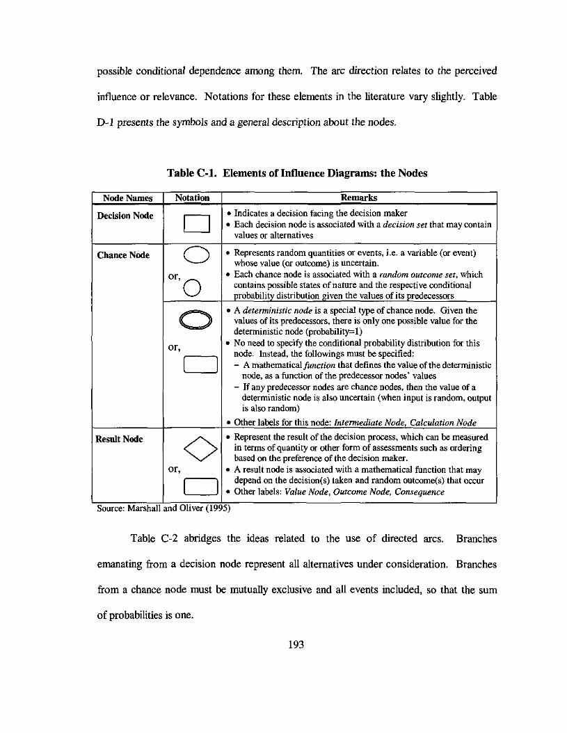
possible conditional dependence among them. The arc direction relates to the perceived
influence or relevance. Notations for these elements in the literature vary slightly. Table
D-l presents the symbols and a general description about the nodes.
Table C·l. Elements of Influence Diagrams: the Nodes
Node Names Notation Remarks
Decision Node 0• Indicates a decision facing the decision maker• Each decision node is associated with a decision set that may contain
values or alternatives
Chance Node 0 • Represents random quantities or events, i.e. a variable (or event)whose value (or outcome) is uncertain.
or, 0 • Each chance node is associated with a random outcome set, whichcontains possible states of nature and the respective conditionalprobabilitv distribution given the values of its predecessors
C) • A deterministic node is a special type of chance node. Given thevalues of its predecessors, there is only one possible value for thedeterministic node (probability=l)
or, • No need to specify the conditional probability distribution for this
CJnode. Instead, the followings must be specified:- A mathematical function that defines the value of the deterministic
node, as a function of the predecessor nodes' values- If any predecessor nodes are chance nodes, then the value of a
deterministic node is also nncertain (when input is random, outputis also random)
• Other labels for this node: Intermediate Node, Calculation Node
Result Node 0• Represent the result of the decision process, which can be measured
in terms of quantity or other form of assessments such as orderingbased on the preference of the decision maker.
or, • A result node is associated with a mathematical function that may
CJ depend on the decision(s) taken and random outcome(s) that occur• Other labels: Value Node, Outcome Node, Consequence
Source: Marshall and Ohver (1995)
Table C-2 abridges the ideas related to the use of directed arcs. Branches
emanating from a decision node represent all alternatives under consideration. Branches
from a chance node must be mutually exclusive and all events included, so that the sum
of probabilities is one.
193
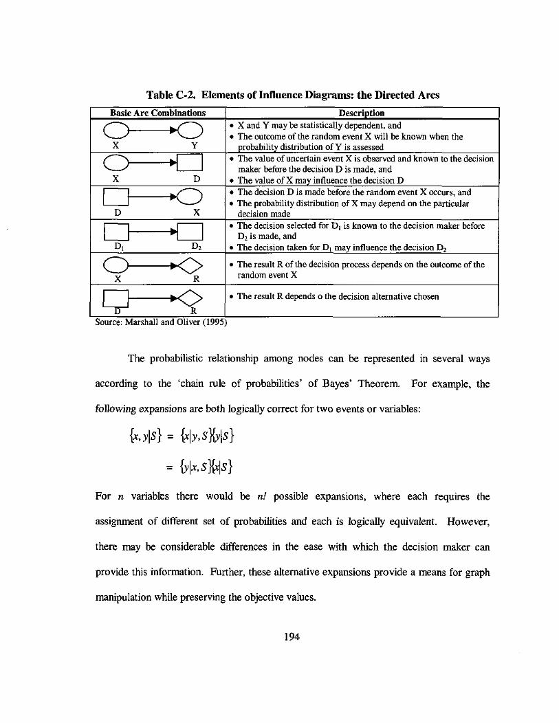
Table C-2. Elements of Influence Diagrams: the Directed Arcs
Basic Arc Combinations Description
~• X and Y may be statistically dependent, and• The outcome of the random event X will be known when the
X Y orobabilitv distribution of Y is assessed
a-----.o • The value of uncertain event X is observed and known to the decisionmaker before the decision D is made, and
X D • The value of X mav influence the decision D
D-----<) • The decision D is made before the random event X occurs, and• The probability distribution of X may depend 00 the particular
D X decision made
D---+D • The decision selected for D1 is known to the decision maker beforeD, is made, and
D1 D, • The decision taken for D1 mav influence the decision D,
0-----+<> • The result R of the decision process depends on the outcome of the
X R random event X
y-------.<{ • The result R depends 0 the decision alternative chosen
Source: Marshall and Oliver (1995)
The probabilistic relationship among nodes can be represented in several ways
according to the 'chain rule of probabilities' of Bayes' Theorem. For example, the
following expansions are both logically correct for two events or variables:
{x, ylS} = {xly, S}{Yis}
= {Ylx, s}{xls}
For n variables there would be n! possible expansions, where each requires the
assignment of different set of probabilities and each is logically equivalent. However,
there may be considerable differences in the ease with which the decision maker can
provide this information. Further, these alternative expansions provide a means for graph
manipulation while preserving the objective values.
194

C.S Evaluation Procedure
As previously mentioned in Section C.2, there are two ways to evaluate an ID.
The first method is the Node Reduction technique, which involves graph transformation
that preserves the objective values. The second method is the Decision Tree based
approach, which requires a transformation of the ID into a similar DT representation.
However, there are some pre-requisites before an ID can be evaluated using any
of the above evaluation procedures, even if it already represents a well-posed decision
problem. In addition, there are some nodes that can be eliminated without affecting the
objective to be attained in the decision problem.
Marshall and Oliver (1995) state that an ID can be evaluated directly in its
graphical fonn if it meets certain criteria to be a Proper Influence Diagram (PID), while
the DT-based approach needs an Extensive Form of Influence Diagram (EFID).
Shachter (1986) defines a PID as 'an unambiguous representation of a single
decision maker's view of the world'. Further, Marshall and Oliver (1995) specify the
following criteria for a PID:
(1) With a single origin node and a single value node,
(2) Without cycles,
(3) Whose origin node has no predecessors and whose value node has no
successors,
(4) In which the 'no-forgetting' principle is applied to all nodes.
An Extensive Form of Influence Diagram (EFID), which is a PID that needs no
arc reversal operations using Bayes' Rule. This means that the ordering of nodes
195

corresponds to the real timing of actual events and decisions in the associated decision
trees.
There are a couple of node positions that needs to be eliminated before the
evaluation procedure, because the elimination of these nodes yields a lower complexity
of the graph without compromising its information content. The first condition is the
presence of barren nodes. As previously mentioned in Section D.3, these are chance or
decision nodes that have no successors. This condition implies that the value of these
nodes will not affect other nodes in the diagram and therefore, they can be removed. The
second condition is the presence of irrelevant nodes, which can be recognized using the
following definitions:
• A decision node in a PID is irrelevant if its only direct successors are decision
nodes.
• A chance node in an EFlD IS irrelevant if its only direct successors are
decision nodes.
C.S.! Node Reduction Technique
This method evaluates the ID directly in its graphical form. The procedure is a
'one-at-a-tirne' deleting node, where the information constraints dictate the deletion
sequence. From the node reduction procedures described by Shachter (1986) and Clemen
(1995), the algorithm can be outlined as follows:
1. Look for any chance nodes that (i) directly precede the value node and (li) do not
directly precede any other node. Reduce any such chance node by calculating the
196

respective expected values, and the value node then inherits the predecessors of the
reduced node.
2. Look for a decision node that (i) directly precedes the value node, and (ii) has a
predecessors all of the other direct predecessors of the value node. If there is no such
node, then continue to step 5. Otherwise, reduce this decision node by choosing the
optimum value. The reduction of decision nodes does not inherit any new
predecessors to the value node.
3. Return to step 2, taking into account following notes:
- Chance nodes whose true value will not be known at the time a decision has to be
made must be deleted before the decision node can be deleted.
Chance nodes whose true value will be known at the time a decision has to be
made are deleted after the decision node is deleted
- Decision nodes are deleted in reverse order (the last decision is deleted fIrst)
4. If none of the remaining chance nodes satisfy the criteria for reduction, and the
decision node also cannot be reduced, then one of the arrows between chance nodes
must be reversed. This step requires probability manipulations through the use of
Bayes' Theorem. The criteria for such nodes are (i) it directly precedes the value
node, and (ii) it does not directly precede any decision node. Afterward, both nodes
inherit each other's direct predecessors and keep their own predecessors. Note that
the manipulation should not create any cycle in the diagram. This step may yield
barren nodes, which can be directly eliminated. Afterward, return to step 2.
197

5. The procedure continues until only the value node remains. The value node then
provides the decision-maker with the net valuation, and the optimal strategy can be
constructed from the details of the deletion of the decision nodes.
C.5.2 Decision-Tree Based Approach
The second evaluation method is Decision-Tree based approach, which initially
converts an ID into a DT. The evaluation is performed in the DT-format of the decision
problem following the rollback algorithm. Marshall and Oliver (1995) describe the
rollback algorithm as follows:
1. Start with no labels on any nodes.
2. To each result or terminal node I, assign a label that equals the payoff or loss at that
node, so that Vi =ri , 1j E R , and R is the set of outcome states.
3. For any unlabeled decision node i, where all nodes j connected to i by a branch (i, j)
are labeled, set
and set di* equal to the decision that yields this maximum value. If the object is to
minimize loss, replace Max by Min, and set di* equal to the decision that yields this
minimum.
4. For any unlabeled chance node i, where all nodes j connected to i by a branch (i, j) are
labeled, set
198

5. Steps 3 and 4 are repeated until the starting node is labeled. This starting node label
will give the maximum expected payoff r* (or minimum expected loss 1*) for the
tree. The di*'s on each decision node identify the optimal decisions.
C.6 Commercial Software for Implementation
Some commercially available software can be used to aid the modeling of
decision problems in ID and perform the evaluation procedure, provided that the above
pre-requisites on structuring the decision problems are met. Table D-3 shows selected
software that uses ID, either as its sole method or combined with other approaches.
This research selects DATA™ version 3.5.9 for the following reasons:
• The software accommodates both ill as well as DT, and conversion from an ill
representation to a DT can be done with no trouble. This feature provides helpful
corroboration during the process of model building, since these two approaches have
complementary features. While ill is useful in simplifying and presenting complex
decisions, ill representation shows detailed ordering of the nodes.
• The price is relatively low compared to other software with similar features.
As previously mentioned, there are slight differences in the node symbols and
other notations across the ill literature. This remark is also applicable to the computer
software. As a consequence of the above software selection and to provide groundwork
for the ill representations in Chapter 5, it is necessary to put forward some features and
conventions used by DATATM:
199
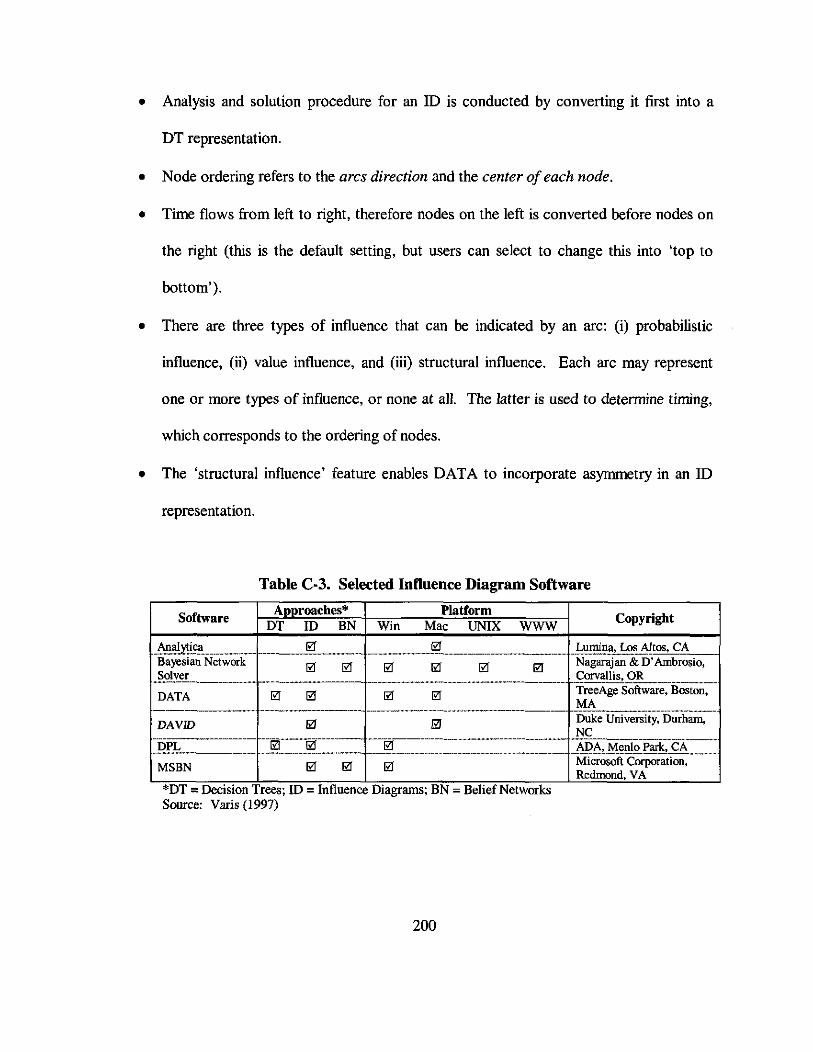
• Analysis and solution procedure for an 1D is conducted by converting it first into a
DT representation.
• Node ordering refers to the arcs direction and the center of each node.
• Time flows from left to right, therefore nodes on the left is converted before nodes on
the right (this is the default setting, but users can select to change this into 'top to
bottom').
• There are three types of influence that can be indicated by an arc: (i) probabilistic
influence, (li) value influence, and (ill) structural influence. Each arc may represent
one or more types of influence, or none at all. The latter is used to determine timing,
which corresponds to the ordering of nodes.
• The 'structural influence' feature enables DATA to incorporate asymmetry in an 1D
representation.
Table C·3. Selected Influence Diagram Software
Software Aooroaches* PlatformDT ID BN Win Mac UNIX WWW
Copyright
AnaIyti~!, ~ ~ !,Al_~-",~~_~.f,!tos, C~-c--
Bayesian Network 0 0 0 0 0 0 Nagar.jan & D'Ambrosio,SolveL. _. . .___________ .Qrrvallis,.9L _DATA 0 0 0 0 TreeAge Software, Boston,
1-. __. ._. ..MA ------------------------.---DAVID 0 0 Dnke University, Dnrham,
NC
*DT ., Decision Trees; ID - Influence Diagrams; BN - Belief NetworksSource: Varis (1997)
200

C.7 The Base Case Model
The structure of the base model in this research is shown as Figure 5-2, copied
below for easier reference:
C4,ReserveCapacity
FI,External
Information
01:Invest?
Figure 5-2. Uncertainties and Major Decisions in the Base Case Model
1. Fl:
2. Dl:
A forecast or estimates on the existence of geothermal potential, provided
by the government. This preliminary survey cost the least amongst test
methods, but it has the worst accuracy.
Potential investor needs to evaluate the available information, which is
from the preliminary survey. Alternative decision at this point: (i) Invest
if the information indicates the particular site is prospective, and (ti) Do
nothing otherwise. This situation can be seen as an investment option:
201

3. C1:
4. D2:
spend the cost of reimbursing the government for the preliminary survey
data, and acquire the right to review the information and make subsequent
decisions accordingly. The payoff for this option is a right to continue and
obtain another option, which is the right to explore the prospective site,
provided that the potential investor and the government can reach an
agreement on the price of electricity to be available when the power plant
of this project is ready to operate. The price determination would involve
some specification requirements as well, such as the amount of obligated
purchase by the power utility company (Kahn, 1995). This obligation to
purchase is commonly known as the 'take-or-pay' term. Another
important terms that are embedded in the price determination are the
lifetime of the project and the capacity factor for the power plant. The
latter refers to the amount of energy generated from a power plant relative
to the maximum possible energy generation.
The possible outcomes are: (i) agree, and (ii) not agree. In a successful
negotiation, a price and quantity of purchase are agreed upon. Otherwise,
no such agreement would indicate that the option obtained at D1 is not
exercised, and nothing happened or the option expires.
The incoming arcs are from D1, C1, and F1, and these three nodes are to
the left of D2. These structures indicate that the decision D1 was taken,
the information known to D1 is also known to D2, and the negotiation are
concluded. All may influence the decision at D2. If the prospect is
202

s. 03:
estimated as a good one, and negotiation is successful (there is a price and
purchase quantity for the future electricity), the investor must make
another decision from the following alternatives: (i) explore the site, or (ii)
do nothing. When exploration is decided, then the investor must spend
exploration expenses. Otherwise, the project is abandoned.
Node 02 contains an option, where it would cost the exploration expenses
to obtain the right to a completed geothermal facility that includes a
developed geothermal field and ready-to-operate power plant. Hence, the
payoff is yet another option, namely the development option.
There is a possibility to have another option at this point, which is the
option to wait. This option is present when there is a leeway in decision
time that does not require the development decision to be exercised
immediately. However, unlike the other resource extraction decision,
there is no more information to be acquired at this moment. As the selling
price is known and the guaranteed purchase quantity has been set, then it
would be better to start the operation as soon as possible such that the
recovery of the initial capital outlay can be initiated. Hence in this case,
the option to wait is not appealing and therefore, would not be considered.
The arc from Fl indicates the 'no-forgetting' property of an influence
diagram, which means that this information may influence the previous
decision at 01 and 02, and these relationships are 'remembered'.
203

6. C2:
7. C3:
8. C4:
The possible outcomes of this node are: (i) good, or (ii) bad. The first one
refers to the condition where the exploration activities yield proven and
feasible reserves. The second one indicates uneconomical field.
In the actual geothermal project, this node corresponds to three stages of
activities. In addition to the preliminary survey, there are pre-feasibility
and feasibility studies. The test sequences reflect increasingly better
estimates but also significantly higher costs. There are usually reviews
following each of these tests, which shall decide whether or not to
continue the searching given the exploration result up to that stage.
However, Model-O regards these exploration stages as one lump of
activities to simplify the model structure.
This is the final search for figuring out the size and characteristics of the
reserves and much less in significance than the exploration stage. The
main activities here are to drill operation wells and construct the power
plant. Hence, the arc leading out of C3 indicates that the reserves size and
characteristics are considered as known for certain based on the series of
search outcomes, and the facilities are ready for operation.
This node reflects the true state of the reserves, which may never be
completely revealed. The arc from C4 to C5 indicates that there are some
drilling activities required to maintain the desired reserve size and
characteristics.
204

9. C5:
10. C6:
11. C7:
12. R:
This is an intermediate calculation node, containing necessary formulas to
yield the specified amount of electricity production. The arc from Cl
determines the amount of quantity to be supplied to the utility, while the
arc to C7 indicates the actual supply.
The actual demand by the utility.
This node is an intermediate calculation node. It contains the formulas to
calculate the revenue earned from electricity sales.
This value node contains necessary formulas to calculate the ROE
Table 5-1 is copied below for easier reference. It summarizes the classifications
for arc assignment on the structure of the model. The use ofDATA™ 3.5 allows some of
the arcs to be removed, such as those assigned for the 'no-forgetting property', because
the software has an internal mechanism to automatically recognize an appropriate
structure. However, Figure 5-2 presents the whole sets of these arcs for the general
readers.
Figure 5-2 captures the present condition in the geothermal project in Indonesia.
Some problems pertaining to this setting are as follows:
• The price is set at CI for the life of the project, whereas at that time the estimation of
reserve size and characteristics is very poor. High uncertainty on the resource
presence and quality, coupled with the associated risk of losing large amount of
capital that is required to search and proof the estimates, have caused investors to
205

demand a high electricity price that range from 150% to 200% or more than the other
base load supplier.
Table 5-1. Notes for The Arcs'
Reason for arc assignment Relevant nodes
Input for a decision
Cost components ofROI calculation
._~~le ~cJsio~:~lO'q?E()P~!!Y_~_____________ _No-forgetting property"
DI ~ D2~ D3-----_._--_._-_._-----_._,..,.._,-,_.__.~.
PI ~ D2PI ~D3_._-----.•._-----."...".,..•.•,-------,-_._------.__.-----------".-.....•......._-".-_._-- ..__._---_._--_..",,"..__.•..........__..------
Imperfect information (in the form of forecasts, Fl ~ C4estimates, or tests) that will be used to represent the C2 7 C4true state, since they are observed earlier C3 7 C4
F2 ~ CIP2~ C6---_.__.•._--_.__..-.-.-.- ,.".•.",,-,,".-.•.__._-_.•.•.__._-_._---_.-.•.•.," ......•.•.•.•.•_--_._---- ._---_.•.•._-_.__._------_.•.•.." ..•.•.•.•.•_.FI ~ DlCl ~D2Cl ~D3C2~D3
F17RC27RC3~R
r-,----.-.-.---------------...-.-.-.-.-------.-------------------......---------- _f~_~_~ .__._._._.__Revenue component ofROI calculation C7 ~ Ra Specific description, in addition to the generic remarks stated on Table D.2. Pairs ofnodes and arc that are not listed only have the applicable generic remarks.b Defmitionl-(ii), Section D.2, Appendix D, Definition l-(iiil, Section D.2, Appendix D
• External adverse situation that cause electricity demand to drop have put pressure to
geothennal electricity. The obligated purchase had caused tension, since the utility
are obligated to take the amount but carmot afford to pay. After a long stalled
condition, some of the parties agreed to renegotiate their terms of supply. An early
result of this renegotiation showed a much lower price (US Embassy Jakarta, 2002).
206

This fact has stirred debates as to how best to accommodate the interest of both
parties in the future arrangements, considering the following arguments:
o If exploration efforts can be done in a more effective and efficient manner (best
available technology, experienced engineers, etc) such that investor can obtain
better reserves at a much lower cost, then the 'savings' from the original estimates
of exploration costs should be regarded as a positive achievement. Therefore, this
shall be seen as a reward to the investor, and they have the right to keep it because
they earned it. A price reduction after the exploration is seen as a punishment,
since this affect the cash flow projection that would distress project performance
to the lender.
o On the other hand, the government sees that the high price previously agreed
because of the high uncertainty was no longer appropriate. After the exploration,
the uncertainty regarding the presence and quality of the reserves are largely
resolved.
C.S Model with Two-Phase Negotiation
Figure 6-1 is copied here for an easier reference. A model with two-phase
negotiation is the proposed arrangement to overcome the existing difficulties. The main
difference between the structures of this model to the previous model is the presence of
node C8, which allows the investor and the utility to renegotiate after the exploration
stage is concluded. The new setting is as follows:
207

FI:External
Information
Figure 6-1. The Structure of Model with Two-Phase Negotiation
Cl: Knowing that there will be a chance to renegotiate the terms of the project, the
price detennination at this moment will be to set an upper limit. This capped
figure may be tied to the avoided cost for the base load supply. Using a
benchmark such as an avoided cost or a least cost reference in the base load
would assure that geothermal electricity enters the system at a competitive price.
C8: There are three possible outcomes at this node:
208

a. If exploration outcome shows better reserves than or equal to that previously
estimated at the reconnaissance stage, then investor can select to either:
• Stick with the previous terms: price aligned to the capped figure, and the
quantity as detennined before
• Offer a lower price but demand a higher electricity sale (can be by higher
capacity factor if possible, or a guaranteed capacity expansion) in the
project. This alternative maybe of interest, since the investor do not need
to spend a new exploration expenses but can earn more because of higher
amounts of supply.
b. If reserves tum out to be worse than previously estimated, then investor
abandons the project.
There are opportunities to improve the project value by exercising the options that
possibly interact with the infonnation from these nodes. Note that there is an additional
option in this setting, which is the option to expand as one of the possible outcome of
node C8.
209

APPENDIXD
SIMULATION INPUT-OUTPUT
Contents of Appendix D
D.1 Inputs for Geothermal Electricity Model (GEM): Base Case
D.1.1 Basic Project Data
D.1.2 Data related to Well Perfonnance
D.1.3 Field Fixed Costs
0.1.4 Field Variable Costs
0.1.5 Gathering System Costs
D.1.6 Power Plant Main Data
D.1.? Financial Parameters
D.1.8 Project Financial Oata
D.1.9 Royalty and Taxes
0.1.10 Depreciation and Amortization Parameters
0.1.11 Payment Fonnula
D.2 Simulation Results of GEM
Table D.2.1 Financial Projection for 110 MW, Base Case
Table D.2.2 Financial Projection for 110 MW. Smaller Well Productivity
Table D.2.3 Financial Projection for 165 MW
Table D.2.4 Financial Projection for 220 MW
Table D.2.5 Financial Projection for 220 MW, ROE> 30%
D.3 Real Option Valuation for GEO-110 Project, Smaller Variation in Field Data
D.4 Real Option Valuation for GEO-110 Project, Larger Variation in Field Data
210

D.I Inputs for Geothermal Electricity Model (GEM): Base Case
D.Ll Basic Project Data
_!:':'!l! Gr_~.~.gll:Jl~~it.L. __ __ . }}9__M."Y .
~~;~;:ali~~~;[~j?i=-··::::::::::::::::::::::::::::::::::::::-~~::::~~~:::.::::::::_Q~l:'!?p.II!l:'!1tQ!!rll:~iQl?:_. _ .._.._._~_ ..Y.~E~. ..__Total Operating Duration 35 years
of which: partial capacity period 0 yearsfull capacity period 30 years
f-_. __ .......__ ~~!!J.l.i.!!g£IIE"pity~i~ .__..._._.? ..X~~.__._._Capacity decline after full capacity period 50% per year
D.1.2 Data related to Well Perfonnance
Number of exploration wells 5Number of exploration wells usable as 3
Productive wellsDrilling performance during Exploration 4 Maximum number of
... _.__. _l:~!9_I:ll:!?!1'_~ell~.p."':.y.~.__.~.Y.l:'~.'~gl:'l?L~t.!ll:L~~11 P.!()(!!!~!io.!! _ L_.~__..__ --;c--
~.~!!~~.g~"':~~.g!'paci!y __ __ ?'!"~,,~£~.~.l?!f!!llcapll:c~L__.._Ratio of ~!:()(!!!~.!!v.eIlJ.lIprod!!£ti':,,_~,,1!~.._ _ -±._._ _._ ..__. .._.._._ _.~"-e!!'ll~-.Y.<"'!'~!y decl~".<:>fJ?~()(!!!£~9P_~ells _........~.'!" p.l:!)'~!._._.. _.._..... __.Ratio O!..~E()(!!!~ti.Y~l:':!lIjectic:>.n.~l:'!!s __ __.__L.._...... ._. .._Dri11ing performance during Development 6 Maximum number of
develo ment wells er ear
D.1.3 Field Fixed Costs
Total Costs (Million $)Year Proiect Stage
Surface ExplorationAnd Studies
3
Access andLand Rights
5
...1..... Explor!'~ion. _._ _..?Q'!" ._ _~Q'!" .._ _...1_.._.._ EX.E!()ration._ .__ ?Q'!" ._ ..__22~_ ...~ Devel()p~"J.l~.._. _ __._....... ~Q'!~..__....±.. .Q.l:'Ye.!opment.._. _ _._ _ _ . ~2.~ _5 Development 20%
D.l.4 Field Variable Costs
Drilling cost per well
211

Administrative & Engineering costs
_Q',I_t:ing EX:E!~~tion 8:.Q.<:\,~I()l'l!J:~rl!_____________~Q~__ ___During Operation, as a % of Total Investment
-i5Ufj;:;g:Operation,-as-;;-o/;-ofye;;ay-Cost---------lO%--
___ _ _ 0l'.er.~tion & ~~~!~'J!l_rl~<: c_o_s~_____ _During Operation, as a % of Total Investment 2%
Generating System costs*Per productive well 0.72 __ Million $-Per-make-:up-weii------------------o."3ij"----Mlfii;;n-$-----
*Specific cost to connect with each productive well
D.1.5 Gathering System Costs
Total Gatherinc System Cost: 12.24Yearly Disbursement:
Year 3 Development stageYear 4 Development stageYear 5 Development stage
D.1.6 Power Plant Main Data
Million $
20%30%50%
GenerationPlant
TransmissionLines by
PLNTotal costs 95 0 Million $1----'---- ----------------------------- ------------------------- ------------------------1-----------------------------------Administration & Engineering 10% 0% % of yearly investmentduri'p~_Construct!()rl _Administration & Engineering 2% 0% % of total investment~~O~rat~___________________________________________ _ _
Operation & Maintenance 2% 0% % of total investment
]J;~~M~~~~e-~::=:== ::==:3~:::__ ~- ~=~::=~~=:===_ =o~?_s:s:~~ll_a~i!i=:~:=Unscheduled Maintenance 3% of gross capacityTransmission Losses 0%
Yearly Distribution of Costs-.--------- ------ - ------------- ---------------- ------------------------;---;---1
Year Proiect Stage MW Installed Generation Transmission, Plant Lines by PLN
212

D.1.? Financial Parameters
Discount Rates
Inflation
D.1.8 Project Financial Data
PLN 9%.-"-"-"-",",......•.....__.•.•.•.•.•.•.•.•.•.•.•.•.•.•-.-.-.-.-_.............. '.".'•.•.•.•.•.•.•.•.•.•...•.
_G<:l1!1I'~I1>,.(fi<?l!!L ... _.__ ._ ..___.~Q~_ ... <::'°.l1!!'~.I1LW!,~..<?rpl~t).._. ....~Oo/':.__ .G~~nt 5%
3%
Interest_.__._------- _._-_.._....
Constant CurrentMoney Money
Duration(Years)
Share
Soft Loan Terms: 1%."•...........__._--._-_._---_._----------,"-"., _,......•._"."------_ __.__._--_ -'-'.'--" ...........•...- .'._----Field Loan 3% 6% 15
··---po~e;-Piani·Loan---I---··3% --6-%'-- .-----.T5---- .Commercial Loan Terms: 99%.•._,•.•.•.•.•-.-.-._-----_.__.,-_._-_..-.".,.....,-_.....•._---,-_.•.•._--- '.'.'--'-._-_._-_.•.•.•.•- .-.-."'"" •.•.-_.. '."."." ..'.'.'.'. '.'--'.'.'.'.'.'.'-.•.-
Field Loan 8% 11% 10.•._,-_._---_..-.,----_.•.•.•.•.•._--_._--_ _.-"-"-.-.-_." -.._..__.._.•.•.•. _•.•.•.•._..__.•.•.•.•.• _•...._.•.•.....• ,.,..
Power Plant Loan 8% 11 % 10*For example, Export-Import loans
Debt/Equity SharesField investment covered by Equities or Internal Cash Generation, other 11.05%than for Surface Exploration & Studies, Access & Land Rights,
_l?:,,£!~at.<:J~_J21:!!Ii!J.g.~~.~clJ:Il!.l1\~!,:~_~~on ~ E!1gi!J~r.iJ1g ...__ ... ______ ... _. ____._ ............ _Field investment covered by Equities only (up to Unit I commercial 42.56%operation)Power Plant investment covered by Equities or cash flow, other than for 11.05%
~.dmil1\~!,:,,:~~e and.?I1~i!J~!.~I1~ .._.________ .... _..._............._....__._.. ____..._____..____...___ ...._....._Power Plant investment covered by Equities only (up to Unit I 19.14%commercial operation)Total investment covered by Equities 27.81%
D.1.9 Royalty and Taxes
f~~L--_--..----~~%.-j
213

D.1.l0 Depreciation and Amortization Parameters
Constant Balance Declining BalanceGroup I J Gfoup Z-IGroup 3 I oroup 4 Group 1 GroupZ Group}'I Group 4
Operating Depreciatiorlgate .}?~reciationRate Total.Expenses 25% --I 12.5% 6.25% 5% 50% 25% 12.5% I 10%
..S.l,Tvice Period (rears)... Service Period (years).._._._._._._._._._...0=. _.4 8 16 20 4 8 16 20
Surface Exploration & 100% 0% 100%
~es .. _. ..._--- .__. -_.•. '.'--'.'-._-- _.
.~cess & Land Righ,~ 100% 0%"-'.- .. _--- 100%-_.•.•., .. -
100%-~~ra!!onWells 70% 30%..__.- .- ......- . --_.•.•.__. _ . .._._._._.=~Develqp.'!Jllnt Wells 70% 30% 100%...- -.•.•.•.•. - ...•....•.•._--- .,.._--_.•._.•._- - ._.
~ake up W~~s __. 70% 30% 100%._-_. .__.•.•.__.__.......... --_._-_•.•.•.•.•.•. .._-_._•.•._--.-.~hering..~'ysterns 0% 20% 80% 100%
' •...--.•.---_. -_.....•. .
Gatheri.ng Sys~1!!~xtensiq~ 0% 20% 80% 100%--_.....• _. . .•.•.• ." •.•._-Power Plant 0% 10% 10% 30% 50% 100%-_..... ..•.•.•
100%_ .•._-,. - -_.•.•.•.•.•._._-.-- . _. -_._._._-_.._='---
Transmission Line 0% 100%
D.1.l1 Payment Formula
Generation ComponentCapacity Charge Rate* 20 $/kW/month
r-£l&M C~pacity--Charge Rate - f- $/kW/mo~iF=~
Duration of Capacity ChargeRate 30 years'CCRs are inflated up to start up ofpower plant, and fixed after that
Resource Component_~ner!D' Charg~g~!~~. .. 0.0331 $Ik~...__I O&M Energy C~.!g~. R?:t~ 0.007 $Ik\\ih
Duration of Energy Charge Rate 30 years*ECRs are inflated up to start up of power plant, and fixed after that
Other parameters: Plant Factor on Gross Rated Capacity:Take-or-Pay Plant Factor:Reduction ofECR for energy above Take-or-Pay level:Years from start to transfer of the plant:
214
85%80%50%30

Table D.2-1. Financial Projection for the Base CaseCapa~it)' .110M\N: targ,'?1:iIl.9m~imum ROE}O%
INPUT FROMDATA35 USER:
33i 37) 331 39 401
13.31 13jjf i2.7'-- 12.5' 12.213Jj 13.0 i 12.7 12.5 12.2
6.7 : 6.91 t.L~-~ __L3_ 7509 o,9T 0,8: 0.7 057.5 ' 7.8 ! 7,9 : 80 80
5.7 ' 5.2 i 4.9 ' 45 '"
3526]
i.iil26,'13.676.3
57.3
17.9....!J.19.1
92"7""3.2:;ii:1sj-
653
Co, Discount RateTaxesRovah
Inflatitm
Project V81uefRetum on Equity 30.01%1_ __:~,§,~,,[Ii,I,I~~t:! Sale All No Sale
centsMooWh 74.74 0
,.JLevelized Price 6.1~1 ~~*~~~~~--:-:--t. __._-~:~_ ._,._.,_!!.o~ :~~~tFCF No Sale 01 n:lreExIC-oSi------;--~-640 --"-- -.Q~40
,
7 8'F:J.7 '29.7-3}' - 3.12Ed : 26.1"'53ft -S.l64,8 . 65.0
2"73.0
26'58
64,5
"S.l '6,9 -- iii) 9,024.1 18,1 . 14.2 12.232.2 25,0 ; 22.9 21.2
32.3 397 42.1 44.1
0.0331'"(ilii7'1
5 ,4'
,--32
-Summa':OfFrBB~ Flow:.PV of Exploration Period {yr 1-2L ._.mPV of Developme~~_E'.!r.i.!!.~" r -.1.!:§l".p'y_~,f'_rQ~_':!~ttonPer!~,~_U!..?:~L J-"-,-~~
Total Value ota com Iele ro'at! 41.67
o
,
PROJECTED INCOME STATEMENfiUsf MILLION)
GfII,CALClIL.:4nOl\lRESUlTS, reaminged:
1. G:ll;p<ll:~YG:hll;I1I.!il'l:i2. 98.i.1l.:CilP~~JSharges3. "R~~~lJl1::fll.:hll;!gl!:4. O&M Resource Charge5. Total Revenues
10. OperatJng profit 15"s1, 10,4), (.4.6) (10.4)1 116.21: (12,6)' (15.-4)
JJlrllfl!~JI;,~Pfl,Il~~~jIT?J j 1 (15.~) (1:(6)1 (1},~:(1?Aj['12. Imerest Income i13. 1l11al Other Income (ElCpenses) (15,5)' (14,6) (13,6) (124]
(OUTPUT SUMMARY:
"S'g'mm-ii.v0iEXii8ndltUr9S: IPV of Reimbursement Dr Signature Bonus
____. ___",,,,,,,"'.,_ T,f'i __Rl!i'!lbursernent or Signll;l:lJrEl!:l9IllJl:l 0,4,7. CJp'?l:<lt:ftlgF;_~~_I!§I1.€; Ae;)1P,~"i 16.2] R~: 15.4B. Depreciation and Amortization I· !9, Total Cost of Field Prep & Electricitv Generalion 0.4 4.6 10,4 1 16.2 I 12,6 : 15.4
I
:Generatina Capacit!!!~ctetil?nary Plarrt Fecior:Take-Dr-Pay PortionReduced ECR
28.6" 31.7 5ij' 57 5.2 : 4.91 ',5 '"0,' 13 2,3 02 0.2 i 0.2 i 02 0,23,3 "9",5 . 17.2 "Ti1'" 1.6 i '1."5: 13 103"
24.8 209 37.8 : 38 3.5 : 3.2 i 30 2'"
__ ?!3,§T jfY _ -Si~_: 5.7 : -5.21 4.9 1 45 '",'i.'l5"" --- ---~----,-.-~-~
15.9; _~1] _____----:-=-§?)~ §·L §,:?i 4,9 4.5 ',2
'Q,I, 44.1 , ~.3: 5.7 : ?:?: 49 ',5 '""i' -56".":3] 58.5 : -6.6-'- 6,1 56 5,2 V39]57.9
25217,6252
32.356'
16.8 252
16.8 :42.8-:~§,C!L_
(15,4)
(154)595
(1§Al(15.4)
(126):
(126)442
(12 6)('26)
(162)1
I(162)1(162)
('6)
(45) ("'4)(,,6) , 00 ~)I
~,,)I
~:4),~,~)
1Oc'll _,~, (4,6)~ -!10:'C - (16 2)__~4L 5,O 15.4! 31,6
":??,t:::!:lrr::l::~rrljllg~elf~!eI,'mElrElstillldT~;I;J11:11~,I::.I;lIlP~::E:"ilf1l,I:IElf,lllt,I'u: a,nd Deprec [10]+(8;
:H,~e1erC)!il~os:se~ Befllrl:!J<I;I;(tIlPIlfl)J~(]+'31J.~:~~y.<I~y"j?1-;~<I!!1,,~~~,L"L --_.':16, Income Taxes 121'"company lax rate!17. Net Profit (Losses) After TalC (HPAn 114·1s.16) (0.4) (4_6) {10.4)i (16.2)] __ (12.6)) (15.4)
'T$'·",,~,,'~-r;;i'~'(i:~~'~'~'~j"$i4~r~-Tal(NPB111~~119. Losses Ganied FOlWElrd '20. Rscovered losses'21.Net~@,~~-!"~~9~~es"C'arried'j:o·~·
215

Table D.2-I. Financial Projection for the Base Case (continued)
PROJECTED CASH FLOW (IJSIMILUOHl ..------,--....".--~·I--.,__-_..,--_.,,_"--~-_'""'0' 1 2 3, 4: 5: 6 7 a!,-- ----- . 4013933;
1.5: 1.3" 1.3
6.iT i:J.2~:?8.7 8.8 : 8.9 :4.0 ' 3.6 : 3.2
31
1},i:l;
6.9
~-'§.-'
0.2B.i"U
35: 36
-~---
7603) 13.3
'17.91 6TI
'V.2'! 1.7
2.3 . 0237.4 ' 8639.0 : 4.7
9
65.3
9.0j":,2':'4"9.5'
--'-:3 .32.233T
55.0 I
8.7 113.6 j
3.3 ;
---_·:······10.4121.5 :26.0
43.3 39.1 :
6.914.6'
23.640.9
64.5 54.EJ
i~:~115.4'16.~ +--,_._ 12.6'____..__~§__ 10.4:
:C.sh~~~~9pl:t~lo~'Cash In:~~{ - ,~,~,~~,,~~rT,¢~il~(;tjonofRe~'~'~~~2~r--Cash Out:
,?? Ope~i~g,_~_·p~ij~~~,I~}26 Il1t~rE!stFl~Yrn9nt {15},2L_I~~_o_~,~"f~.~~l,_28. Insurance_29. ROY"y]15] ----- I --' I30. Tolal Cash Out [25+ ..+301 I 4.6: - 10.4 - 16.2,12j5 15.431. Net Cash From Operation 124..::01 (4.8) (10.04) (16.2)' (12.6)~
-. ~~.
,G~~~~~lotiimteslilotgCash In:'CsshOUi:- ",' ," "" """ '", " ""'" "" '" '32. ~eirnburse'!1ento~$igij,~l~riBonu$ (I:I~lOA ~ I33. DE!VeJ~pment&-Construqit:ll1~-t:l~-~J~J - --or 0.7 i 2.827.5T' :36.1! ~i4 , '"'34. _t::_~e.l~~"~~!j)!'!.ditu~.~{031 _.' , .. ~":"_,,,,L~ _M'''''''' • • __, •• " '''' ,,0.8: 0.8! O,~35. Total Cash Out 133+34) 0.4! 0.7 2.S 27.5 i 38.1 63.4 0.8 , 0.8' 0.936 Net Cash From Investing [cash in· 351 !D.4); tU.7) R8J (27.5)1 @B.n (63.4) tU.S): !P.S) !D.9)
:~~",!:,~rn Fln~Ill::illgCash In:~,~quitYFiI'f.'!!!rif"@r,,,,,,,,,,,,,,,,,,,:,, ~~'..ze. LOiltlQ~~9 (Soft &(;~rrtrt!~~<lrllUJ,!,~,?J
_~--,-_ .. }~!i119i1~,h..!tl_.@r.:t:~LCash Out:~,~i1tle~tl~ipalR:epaYrTl~r1f,H~:l~J"41. Tolal Cash'Oull401 '42. Net Cash From Financinq [39-41
. 15.3 j
5.3
l}}L
13.3 9.3 45.1
16.140.256.3
56.3
EJ67.1
67.1
..._.__1.__
~.9,A",,;10.4 i'10.4)1
11.~~ ".11.5n
43. Net Cash CtIanqes 131 +36+421 4.9 : 8,0 : (3.9) 1.4 : ~-(11.7l 31.6 I 33.9
27.8':" ,~l._~!..,~..J M,,~J)
"44. Begi'nn'in'g"C~5hEfala"nc'~
[4~,~~,!,~,i1,~h..9~<l"~9!!..F~""46, EtlditlB(;<lS~,,~i1f<ltl~~H:~~~L
~"~' i.4.9
-~))
80.(3.9)(3.9).
·1
f.Aj.,~.4 i
5.6. (117).5.6 (L' 7).
31.6 '3f6J
33.9'33 9 '
27.8 "'.7 39.0
39.0:39.0;
4.7
4.74.7
4.4 4.0" 36 3.2
44 ,,4..;Qj 3.6 3.24.4 4.0: 3.6 3'.'2'
216


Table D.2-2. Financial Projection for Case 1
!G~p_a_~i1Y,,~~~!'4YV;Ji:lfg~~IJQl!!!plt!!~,IJlR9E
'11tPlfT FROllUlATA3.5 USER:
i~~-ifg~~-,,-·_"··- -J~:II~·~:=:=~~~~i
EXPORTED TO DATAJ.5:
:,~Tl)i.~,:I:!"Y~ltli!__\!-:,,~~,~!I!i~n 1§<i!~,AJII ~~~ale
83,54 0
7~r_!9.~_!.r:@_~_I..P.,,~_duct~i!Ratio of PrQductiYelUnProductive wells
IWel1 data:
Royalt
Inflation~COUn1RaleTaxes
.IReturn on Equity 30.01%1cents$Il<Wh
_,lLevelized Price 4.64[.--0:
!FCF No Sale 01
f!p.!.,:=.~y Charge Rale ($Jk~!~Q.I}th"
Q~ Ca~ Cha~e Rale ($JkW/rnonth
,Summill of Free Cash Flow: USi million
PV of E~,~!!.~t~OIl Period (y! 1-~_ ...,.. -11.06_':'.Y.~~~.~~pment Peri.!!.t!.~ ._.. _ -31.4~
?" of FJ_~~~.~i~_~_e!.ri_'!~-llr~~QL___ ___~,~Tolal Value of a complete project 40.60
0.85
million0.40
I_=::J!·OO31.46
\OUTPUT·SUIlIIlIARV:
Summa'Y of Expenditures:iPV of Reimbursement or S\gn~t~f9 BonustpV of ~~Iion Cosl _.,..,py of Development Cost
Take.Or-Ps.y_Poriion,Reduced ECR
iGenerating Capacit!Oiscretionarv Plant Factor
!Gf&fCALCULATJOHcRESULTS. rearranged:
lJ_:41,Q:~"l 9:1:1].__ 0.00,12.83 8.45 0.09 0.00'
0.00
.Q:~:
0.00'0.00'
0.00:
0.001.
----_.~~~-~.._..
0.000.00.
[0.20): [O69} [1.18)' [1.68) [21B}FCF36 FCF37 FCF38 FCF39 FCF40
0.2 0.2l 02 0.'21 --_.....Q:~,. 0.2
0.00: i:irol ·"·0.00: O.ooj 000 0.00:0.07 0.00' O.t.:)' 0001 0.00- 0.00
42.34FCF35
0.20 '
i0.19 i
7.04 1
--I
36.35FCF9:
_._-_._<
033~?:?~.,,;
I1J:'46"'!
18.210.48'(f.5ij
058(7.39).
0.83: 0.69(8.68) (2i81)
FCF1 i FeF2 il"CF3 FCF4 FCF5 FCF6 j FCF7 ; FCFaj4.59)! (10.411 132·85J (12.77)' (15.70) 45.31 ; 46.30 : 46.16
0.20 020 9:;'Q; Q.?9J d.2i:j' 0:20----:-·
0.58 0.48 0.40 : 0.33; 0.26 lin'(19.01) (6 16)-- -(6)1)- 15 17 12.9f= --'9·14
i4i:'Fr'~~~"'~~~!~~,p~~j
:48. l:li~(;Il~~~t~",:",~~:EI~Eld_~"'G~ (+co~ntri~~~t,,; 0.2i::i'
1'49':' Oiscount Factor for PV calculated at end YO
;~:py~of fCF"~'i"'~'~~Y~,- .....~~ __~""'_"";?J-,-_~J~:~:~!!!~~_IPYl)f'F~F, calc~l;lt~~;lt,~~~,~ __~~~ :i~lJ!l.itjal inve~~_nt ..," ",(I!~L
i~:NPYlJf,p,~J~,g 40.60
!...------------------------------------.-- ..----------------------------------._--_.,.,"""",,",,----------.--'"154. Discount Factor for FV cak:ulaled at end Y1i55. FVOf FCFai'e'ni:t"'Yri""'------: .. '--":1~.~._~__(I..e.·-Totalf'Y'~f¢f:_-c.alctil8t~d··.·~··.·end··'Y1) _~~~~ _~"=~
i$!:_F~r~'£~~_! .Y,~,~,i~,~je(z)fQrjfu§,,~~~!. 0.1~.
l~·~ fttr tIl~l:I~ ~"'~~~~~ -"2.ai'
;~~~~Ij!~~V~'~~~I~(if~~~,~,~g 56'&~: 0.161 z = % C_h!~!U)fpro~£.t¥a.II,l~:::flqR on l_nB"p~jEll;;t
__~=:.!!!. ((pY1:'fGFJYF'YI:JJ '
o 1i 2 3 4 5' 6:ftJ.' Q~~'¢'~'~'s'-t~~~sIk-Wh,nq,mi.~~,ijl . -".--. 0 0; 0: lJ. 0 01 §:~i
i~~" ,y,~~""~~,~~~(~El~~&~-:-reQD"- --- p: 01 0' 0:- 0 0' 5.8311§?, ~zetJCo~_s.(c6nt~\I\Il?,rea)L__ .. i A:~·,', L ; : , L....... ..' ." ..".1[(t'lCll~:not il'l,~'tJ~~pl,t+~pecific ...~.osts.!'~S~"'~,~"'!r~I'I~~ission costs .al'l.~ClPEi!~~,i,l:l,~<iI~QSIS afIe~t~Elpl<1l~!~,;;l,~J!:!l!J~~!~~to PlN)
76.995:l5l3!
B 9:7.01 7.03:5:53--5.39;-
35 36:7.99 0.94:-2:84---0·.32'·
370.979:~_._
38:HOi0.32
39J.~;
__.__ 9..:.~
401.000.32
218

Table D.2-3. Financial Projection for Case 2
;<:apacitY~~Q"MW",~ig_~ng minimumj~'Q,g,,~9%
ilHPlJT FRON DATA3.5 USER:
Rat:io of Producli¥e!Ulioroductive wells
-OAO"
7
No Saleo
-53.54:lT~46
Sale All"9298ID4PreProdCost 53.54
p"n;oeveost---1""f46
EXPORTED TO DATAl.5:Project Value
:US5 mimon
Well data: __'IAveraae initialy.!£.duclion (~L" .. _.__
. ·preE-xpICost 0040
InflationCo. Discount Rate
IRetliin on Equity I 3Jm~
;TaxesRovall
centS$IkWh- lLevelized Price 3.891 --
oIFCF No Sale 01
-1rOO:i2~oo92.9339.44
US$ million-~.!2!.oration ~~!?~Jl:r.l:!l.
PV of Dev.!!.opmenl P~~gd {yr 3-5'PV of Production P..2~Q.~ (yr 6-4QLTotal Value of a cOffilllele proiect
,ISumma'ry"'Ii'j"j:reeC8SiI'Flow':
42.03
0.4011.00
iPV of DeveloDment Cost
:I~.~~Q0:~Orlion'Reduced ECR
10000ljTSUUIIARY:
lsummaiYOf ExpenditUres:''pv qf 8.!!il!!.'?ursement or Signature ~g.':I~s
'pv of E!p.~q!!tion Cost
:Generating Capacit!Discretionary Plant Factor
:GEII CAI.X1JIATIONRESULTS. rearritRg9d:1
CI.&f' -.-jj~~L ".. "D,.fI3.. ..(7.23). (29 39) (8.25)
o,~L .. Q,~;
6.00:om!
0.:2'
0.00'-o.oif
0.00"b".oj'
0.2: 0.2
O~OO
9,l!l].
0.00 0.00:OW ..__Q,QQJ
o.ro'000
~r~:0.00;
0.00am;
o.OJ0.10:
000000
_9-,~------.M._... _0.2
47.26 ~.2O)i IO:EQL (147)1 (2.11) (2.76)FCF35 FCF36 FCF37 FCF33 FCF39---,:a:40
0.33' .~_'_~L~~--~~q)~.,_.
17.23; 14.72 ~".?.1..j
0.40 i20.21""
FCF5 FeFS FeFl FeFa FCF916,02) 50.29 ' 51.46 52.76 : 41.74
0.20 0,;Ij-:'" 020 q.2(): q.;;,:)[i
D.ib ._.Q·~f! p,~,,; [>.'23 ' D.19,:(8.44). 16.84 : 14.36 12.27 8.09 !
0.58 0.48'(7.50). c __ r! 73)
FCF4
~
b.2O .~
i]':'2ij"'"
FCF3
0.69(3527)
FeF2'10.41
b.83"18-00)
-;-
[4.59)'FCF1
......
i5,~~T
39~__ (3.63)
~.40)
39.44 :
;47. Free~"'F'iowp1j4j, .
14E3,i?i~:~,~,~6f,r~tE!-~CI~j~stll'~"W~~",'~~,~~,ry'~~~)",,: O,;!)
!49: Oisco"'uni Faclorfur"'PVcalC"iatedat end Yo9i"'py"o'i'F'CF' at end i(() "'. ,~", ...
:51.~",,(i.~,'Jilt'~fPVlJff~f,t~lc-ul~!~d al en'[j"yt:52 "Initial inVestment - .. -." . - ..---
i$~.~ip\Torpr~j~0-·"
11~{j~iscouriiI!~q~-r,~r .F"{,C~.~~I~Il~,~§l~~"JL",55. PV of FCF al end VOi56:PVj"«("~':"'t~~("py:",~(p~F :.'.~'~lcul~iedSt·"~'~~"'Y)II'
!57. f()~~asIlY~~~bJ!J~l..f~,~,,~~.i,~_~~!- __ -'.- _Q,.!~
;58.~J~riheBase'¢~~i(1,TQj~ -42iij-" "\"""""""""""""._"."."".._..,---."_.---""""""""""""""""",,". """"""""'"""""""""""""""",, """""""".,
i~,~"'f,~~,~,~ylll~llI~I~Jzt€:()J!lP<l~rlg,,~"'~,,~:IJ·~~iz"''l§~~~rlg~,~,f..P~()jt:!~!~Il'''"f;!OR(Jl1t~t:!p~()jt:!,~!,!..:=II1J(I;)Y'!,:'f~F1~)
L.
i
35i 36: 37 38] 39---40'6.70: 0.91' 0.94 0.97 IOJ 1032.33:' ··--·0:32· q)2 . '0.32: 0.32 0.32:
0' 1.1 2' ::I -4 5: 6: 7 B 9)it:!l.·y;,-~·~~O~!s ..(ce.ni:~~iI<IMi,.~~'~'i'~~"Q·· 0: O! 0 0 0 0' ~;'f@' 5.85 5.67 ?,~;" .--ili1:lJ..!1~t~sts'(c~rrts,~,rEl!l.n 0" ~~ 0 0 0 0 i.891 4.76 Hi-4 ·4.!i2!Ig .~li!lldr()~~(C:E1Il1~fI<~"",~,Il~D l .. },~:,JL.. .....:"""",,'L. ..:i~Cl.IS!,:,nCltirl~I,,~£:l!+~p~,,=,~~, C()~I..§~,,~~.h as 1~~"I)§r:!'il:il:ii()rl ..~,()§!I:i"'~rl.~"'l:IP:llration~LIO()~I:i~lln~Elpl<ilI1..t~_<ilre IransferrEl'~J()..':~l"N)
219

Table D.2-4. Financial Projection for Case 3iCapailli 220 MW;. ~l9§ing the average production cost: of theottler base load suppliers, ,,""""" "" _........ . "' , _,._-_.".,.."'.,., ; " , ""''''''''',,., ; " ,
'1ItPUTFROIlllOAT'A3.5USER:
Ratio of ProductiYe/lJnproductive wells
-11.46-.040
No Saleo
-53.501
Sale All- -gi.n_._._~~}:il353.54
11~460..40
EXPORTED TO DATA3.5:f'~()jlll!,~\I~lue
US$ million
.:lreDevCoslPreExplCosl
1·E!!,!pro~~ost
data:".~...!!9!jnitial~,oduclion
Rova~
:cents$Jk1JllhLeveliled Price 1 4.031
: 0FCF No Sale 1 01
InOationco:DrScount RateTaxes
IReturnon Equily 1 31,.41%1i '" I
lSummarvOf"j:ree"C8ShFlow: :US$ million_~~!!p.Loraljon PeriflEJY..!...l:.?L....._, -11.00 ..
PV of D~.'!l.E.f!lent Period (yr~L__,_._. ~_~~
JP'-Ef Prodl!..C!!9.r!J:~od (y~!QL- __._,~,??Total Value of a com lete nroiect 43.68
,py of Develoomenl Cost
iGeneraling Cap<ilcitiDiscretiOflsrv Plant Faclor
(OUTPUT SUUIllARV:
iTak&-Or-PaY_e.~~ion: Rl!rIlJ~l!d ECR
Summa'Y of Expenditures:,ipV of Reim/wrsemenl Dr SiRnatUte &nus!PV of ExplOration Cost ...-
I~- FCFl FeF2 : FCF3 ' FCF.4 ------rcF5 ' FCF6 FCF7 ;(4,59) (10.41) (50.79) (12.931' (16.02): 53.29 54.47 '
0.001'-0.002
02
O.e01"" 0.((11-0.001 c -.0.001'
0.001:.0-.001]
0.((11.0.001'
0.2
0.001':9:,l;Q,~,,;
0.2'
ii'oofQ:O~L __
~1211 (1186) (1.521 (218)
0,001o.mf
FCF37 FCF36 fCfzii" fCf40
o.oJ1iiij5j'"
0.2'02
[J,~_L0.084
0.002 0.002'O·~tf,~li
49.49 0.44FCF35 FCF36
0.:2t:!_:
0.i9;,$:,~",I
!
FCF942..40
O,_~~ __'2.57
O·~_;"'_9·~3_'15.08 ! 9.86 :
fern54.04 '
.Q.:,~ :
028 115.20 i
PAP,21.42
Q:~"
i):3j"'")t:as]
0.48 :(773))
ti.2tJ1
0.40_\@....).
0.20
0.48(25).
0.58'_~·5J1.
0.691(3527):
0.83(ll68f
,-[~'4='~"'9·,20r -""~?9 .--'_:!I2~:1
O.8~JQ.$9· ,(l:~J(3&__ (7~LJ~}9)
iGEM CALCULAllONRESULTS, rearri!ii'iged:
iii. Fre:~,,'~~ FI~p~~j
1¥i;[)i!lC-~iifrtr!!i::~di"!~~,~WAf~I~·cou.lt,ry:ri~~) i
i49. Discount Factor for PV calculated al end '1'0m.py"'llf'FCf"~,,,~h,~,,,Xr:i-----''''''''''''''''"'''--=''''
'?1. ,j=l'I,I()"" (i-.e·I()l<lleY~f,f~,f!,_~<llculat~d-atel~~"'~' 44.08;52~,,~fl.itial investme:nt .... _ .... @,A9J.(?? NPyofproject _~.~~ LI
;5(Q.i§_'=:IJ:l,ltll.Faq.IJ:,~"flJ:,~",!:'V calc!J_1ated at end '(,) ,.__:55. PV ofFCF at endYO:!~(,~"',Q,:,'~:",t~{~ipy~(fCF",',(;aicuiated""3!_~_1),~-XjIf 51':40"'"i~r"[~@~~i~:57~~<lp_lelJ;iflirThis-~as~ ----." : -0.18;
i~;",,"~,,~~_-'he-~~~"'h~~~~ 42'.l:J1'i
i,~:.£()~IiI~~yil~iI~I~(~i~,<l~,~,g,,~_~_~~___ 1 0__ z= %E~,<ll)g~.2!J!~~_~l,I,el,,=.HQH()~t~ep,lUiect
~",=",!I)J(~l:+:fc;f~)Ip'yl:IJ
'm_.'''''' ._. __ m .m' 0 1 2 3i 4 51 6 7: 8:16!J,:"y!)(t, CO~~!,,(£~l1ts~~'~1'l'Jirl<ilI2L . . .J II 6.Q?,,_,_ ,,~Q! l': na :i~1,~n_~G()~!~.i~l!m~~, real) J l : 5.07 4.93;62. ...~li~el,~",~(),~!,~(~el~t~, reaQ ..,"'I..",:4:,I:@LL,,,"'L,,,,,,,,,,"' : ....L .'.(1\J()~~:':IIJ:~il)clud~PIJll::ll:Plll~ifi,~...£.'?sIS such a?~ral1lO:':'lilO:lO:i'?rl£lJ:stlO:. ~!:I~.IJ:~.llIr:tltional .c,?s!~_a~~~,I~lI~ll:lil1tlO: ..re 1r:tlrllO:fll.!!:~~£,LNL_. _
220

Table D.2-5. Financial Projection for Case 4
S~Il!AJt'l ,I'J~ :3,a.!!..,114.78 0
PreProdCost 53.54 61.24 ,,53.54PreOevc-"-,-----Tf46 .., - -- ·11.46PreEXiCO-s-'-----i5:40 .--,..__..-. -:QAiJ
Ratio of ProductivelUnproducti¥e wells
IWel1 deta:A¥e..!!9.ejl'.l.~i.:'!!l!r.~~l!.(;lion
,EXPORTED TO DATA3.5:~~j~~'\I'illue
l!-:!~~ million
0,3-I
Ta1l8S
Rovalt
InflationCo. Discount Rate
-IReturn on Equity 36.62%1cenls$lkWh
ILlM!lized Price 4.641 -o
IFCF No Sale 01
Capacity.. Ch-lilrQa Rate ($IkW/'Il.~m~.Q_~ Cap Charge Rate ($1k~!rnon1h)_l~
§l~Y Charge RateO&M Enemv Cheros Rate
'3ummOI UI rree .........' r,uw, v.,,, ""'""'~
PV..of ~IOri1ion Period (rt 1-2) -11.00
~2-!,!!!!opmenl Pe~~J'id:~ -42.ce~Q.~.uction Period Crr~__ .._ 114.78Total Value of a co lele to"aet 61.24, ,
iPV-~IOra~on'~.!!~.iPV of DB\Illlopmenl Cost
:g,l::lp~jty)~9,M'f'!;tc3m€!~l'lg",m,~PI'"i~~_of <::?I§';;!J,
IIMPlIT I=ROMDATA3.5 USER:
IGel'lerating Capacn'Discretionarv Plant Factor:J"ake·Or-Pay PortioniReduced ECR
,)GEM CALaJLA1l0HRESUlTS, rliartangf!d:
IOLirPUT SUMIUUlY':
!-s"i'mmalY-OfExpend'itUres:',pv of Reimbursement or Signalure Bonus
FCF1 FeF2 FeF3 FCF4 FCF5[4591' (lD.41)' (CIll9l' (12,96), (16,D2)
48,Pi~t;_~~~~T~!~":,,,,~~j~~,~~""'~C ~+COlJ~ry~~~l __ .. ,,0.29 9.2:i\
0,00g,m,
3.02FCF40
0,_2 , q).
O,OO~ "'0.000,01:); 0.00
0.00:·oIif
ii"2!'j
Q:~JO,OJ!
O.oo!Q,~r
4.14T3]OFCF38 FCF39
DOOl),[)},
5.35 i 4.79FCF36 FCF3?
".Qj!j~,,~Q9j0.12 Q."Q~
60.21FCF35
D20
FCF9,50.71 i
"..1).23,,111.79 "
FCFB
D,2815.M
53.88
D,2O
(1:23'12.53
lJ,~
~A[)
FeF7
~
0.20-'-
FCF6
Q':'~'Q,,"l26.37 ;
65.61
0.20 i 0.20 :
- 0.40 'j "Oj3' 0.28". {Ei,A~)j 21.97 i 18.66 .
0.20"""·
Q,?l1 ;---:~ -'He;(7,58) (7,73)
_QA~--;(625)
0.20"
D,58(23."')'
Q,?Q,i
o.ef' 0.69(868) (35~27)
I
Q,~'~i 0.69'
~B3)1 ..(C23)
i54. Discount Factor for PV calculated!5K"'~ of F~E_~",l!,~,~",YO "~_ ' """"""'" ,.!,~:~~Q,e,I~t:;l1 pv ()ff~I".t;~I~l!,~~,~,~~""~,~,,,~fl~)i1l 7856
l~!:~~~~~' ~I~pt~f
~---,-f~!l!,t;~,~,~.y~riable (~~rt~i~t;<I~l! QJ?;
r5ii~'~J{Ji:t!1:~::~~.~~rlj~'~~ ""''' 4.i.o7J
~:"ff)~~,V~~~~i.f!IE~T!!Ii~~_~"~:""""""",,,,_ ~,~',','1I :;,:~!=~<lflgl!CJfptOjl;l&I"<lIlJl!",,,RO~,l?~,,,~~l!P~1;I0i~:::IIl((flV1-tf~F1J!E~) .
J49.j)jSCDunt"'faCJw"iDi'py caJcujaiedai"endYOi5O,-pyCiffCF"'aiB~,~,Yg""",:!§"L,~""""",~~,l!llal ~ of,Fl::f.t;:;llt;lJl,~,~,~""iijin[f52. Initial investment!~"t.,jpy~pr~jl!9
OT---ll 2 3 4 5 Sf
~~~,,¢,i~~.(~~.~sik'Mi,ij~~in~'ij'" f 6.93 ]. ~~~~JcentsJkWh, ~aJ) ..." i 5.80 ;
~Ii~~~t::l?~s (t;Il_I!~V'Ih.J:l!~~Q""L4,64' ...........L,'''''''""""""L_ .. :......: " __•__;;
,,,::~:..Il~t!Il~!LJ~~P!-_t!:~!fi(;(;9~~,, ~.!Jch ~t.!:!llll'l!Jis~i9fl~CI~~1i~Il~()PE!',,~~i()Il~L~,CI,~,~,::;;llfIe!,~~l!pl<ilm!i> <il,t!'!..lliI!I.!!.l!.tred. to PLN)
76,955.i35}
a6,005.51
9'
7.01 1?,;ri'J
358.10
:i!J313:
3Ei~1.4fF 1.510.56- --D.-50'
38'1.55'D,58
391.6T0.9]'
40165
-:,rj,$9]
221

Table D.2-6. Financial Projection for Case 5
.~~p~~ilyi?Q MV¥:~rg~~ri,g",ili~~$§3~~C:::~!::~ prj~~_
'INPUT FROMDATA3,SUSER:
Generating CapacityDiscretionary Plant factor
I~~~.Q~-,,!:~£,ortionReduced ECR
Well data"~vetage initial productiq_I').f.~L. __._. .Ratio of ProductiYelUnproduclive wells 4
EXPORTED TO DATA.1.5:p't:CIjectVlIlll,e
'US5-miflion
-o.~
f Sale All No Sale---158.980
105.44 -53.54- --:11."46
-'--~n0.40
53.5411":4'6
PreProdCosl~~DevCostp"IFCFNo~T- ot
IReturn on Equity I .47.39%1:cents$lkWh
.ILevelized Price I 6:191'0;
-S'umma~ 'Of'Free CMh"Flow': 'U'S5millionfI_Y of.Exploration Perio!tiU.:?L__ -11,06.!:'f..of Development Period)J.r_~ -42.~
_-f~._~_P"~dur;1iOn Period (yr)?:~l__ -.-!.~.98Total V..lue of a com lete ro"ect 105.44
42.013
-~-,- iUS' million
.J!.4011.06
OUTPUT SUMMARY:
PV of Oe'felopment Cost
Summary of Expenditures:leY ,of f(~1I!lburs9ment or~nalute Bonus...E:!__9!.I;:9!Ioration Cost
iGEMCAlaJLAll0N RESULTSiill.mtiinged:
732FCF40
0.21 o.i
o.oo! 0.00Q,,911 0.00
7.99FeF39
o.OJT0.01 i
r
0.2:
8.63 i
0.001-O.On
FCF33
oj'
0.000.01
P,~0.01
9.38FeF37
0.00;0.02
Q,?i
0.00',Q,Q1
10.04FeF36FCF35
86.07
+--- -~:~l
0.2'
i- amI 015
FCF9 I72.14 1
FCF871.83
0.28-:--lf23-"-~~-
2O.05T'" 16,78,
FCF7EIl57
_P-,---2fI_0:jj '
97.59FeFS
0.20
0.-48' :- 0.40 P,~J
P3) __ 39.22_. 26.98
i:l.46' -- -o~rf:-''' 0,28
~.4'1 32 68· 22.49
-.j.-,-~
I0.48 ;~25)i
I
___0.58
_fl.50)
-'~'-~"--O:B3T
[ll.68)
FCF1 FeF2 FeF3 FCF4 ; FCF5
"1183 0.69'(3.83J ~(U3).
H~~fi9
54. Discount factor for PV calculated at end Y155, flYl)[FCF ate-nd'''Y'¢j'''''''''''''""", .'',',',' '_-_~:---,,~~ P¥1,(i'II:I()t<iIF'Y""Fr:::f_,_E~J~-':l!~",II~"~,,II!l,d Y1l
~$!.F~recai~~~·{a!(~~j~(~f~!fh(~"'~'~!>11
47. Free Cash Flow {31.341__ ;-__ i . (4.~~.41r (50.79)[ (12.93)' (16.02)
-48.···Discou~"~~~~~j~~Ii!,~,.Y!j.,¢¢ ••(~~niry"ri~~) ••••1 '" --ij.20~ 0.20
58. PVO (or the Dase Cas9 ('110~ I 42.01~"'-' "'" '-~",,,,-,,,-,~-~,, .........,,":" .,,,..~~ !
"~~:'f'~i!~,y~~~~,I,~".I~j~~-rrlP~~.~g-~"'~"~':"'~=_ ... j.....-.....-: 1.10; ----.!-=-~"~,b,~,~g,~,,t:I(p~j~~lvalue ==,,~QR(JI)_~p~!,~
z = In (~:I:"'~~~)(!?~) ,
:49. [)iscouniFactor'fur PV calculated 'ai'end YO:5£'1. py'off'cfaienifyo"""""''''''T'' """""" ,j~T~~t;:;=I()j~I,py~o(fi::'f.~~I~ulaleli' ~lIri~Y( 105,84'52. Inilial investment - '" "'''',.",. ' --- IP.4Oj'~3. NPV(jfpr()jlll::t 105.44
40225(),~
2.18:-0.69 1
3935 36--3-7-- 33i
10.90 2.00 2.06 2.1210.69" 0.69 0.691
9.331'7.15
919.297.33 :
B7~
9.257.52
69.117,71
5-4:3:2o:~,: ~,~iL¢ij~T~(~~:l1iSll(Wh.~~i1ji~~ij;l!?!· YI'l~Costs (~~fII?!J<Wh.~<lQ, " '"~_~lllIflli;!,~d Cl)~~((;~ntsJlc~"",r!,~,~,.. ....,. 6.19. ._,,,,, . .. _ .. __ ' "'""",,_,,"',_ _ _(Note: not .in,~I~'!~~I!+,~P~.f,!fI£f.l!sts such a,s trii!'sl1"li!l:!l:il)r1(;()St!l:.<lI)~(J,p~@!i9,11~,I",l::l)!l:t!l:~~ __eEJhll!P.l.~!1I!l:il.~L'!r1~erred to PLN)
222

Table D-3. Real Option Valuation for a Smaller Variation in Field Data
223

Table D-3. Real Option Valuation for a Smaller Variation in Field Data (continued)
Node End-of-Period Payoff
··"Rov:/·········..C·iiTumn·-·U··Si'ale·..Tti'ii·wn..si'ilie2 24.212
OptionParameters :......····m·..··....·_..···........··..S..···........ ·. Value
32.160320.3415
27.3138
224

Table D-4. Real Option Valuation for a Larger Variation in Field Data
Base Case PV!.ya~ationinpCl~a~.~~~Ty~_I~_El~: 1DOfo oll_~~<;Irge~"A~YVoll't\lell prodlJ(;ti\l~Y,:2§.9g;~,~.f~~~,,,,,,~llratio
1.2840.779
iii
____~_i
1,~;lI, h:tJ,l:ated _fliu:al'll.eters", i. 'lip_'~-9_~-~0_~-6~,_:p"~~,:~1~p_-:~
2. DQlNn movement per step, ('----- --- -1~·::.8f~:kIr~~f~(~::P:::~-_:J ""---~---
~~~.J
'~1tio/;'
42.074Ol.
25.00%11
_t~.p,~,te"~ra"!~!~_~__ ,,_~_~ _1. Annual risk-ft:ee rate2. Current value of underlying, V,_-~;_~-L~~:"~I~~~j~iDh.i~_~,~~.:_-_:~------'4. Annual standard deviationl.~NurnberofstepsperleaL ...~~.~~....
"",,
--+-_...
i.~~~~. .'~'~~"" ... ~.~~.~~~ ·1
J1~move.rnentP,r~leJ'~~iL28..L ..2. Down movement per step:' 0.779
.- ••_-~ -- -!3·__ j~)~~~.,.pt~.~_:_~:Q_m'fn'a(i_~'!~!.~:(~~I __=__j,;,j,:''1. Annual ri.s.k:fre.e~t'.a1." . 1"100/;'2. Current value of underlying, vi 42.0713E:.erci§~~ri,cj~';{bpii()ri:LL 11.06
1
14.:. 1::_~_~_r_S,i~,e. ..P.!i~!_~~r9.p.uJ:)_t:L) 21.6I~': Wf~_~t()pt.i~r:tJ_~_~r~~r~ ..". 6i~. Annual standard deviation 25.00%:7.Nurnbe~o! step..'..ge!year~ .......L~
1
B~V.lue ors. uenti.,C"ompound Optlons'·- .~~,
]iii l;11_;hi iu,i,.,r.~:',:!, J 1II~llrlrlUlrill11IUi il~l:illllurlm_':::II!m~~. :~~~P5s,4~;:;:n~~~~d '1
I 17.34 .....:!I?,.7:3I.~ 51.51W~2: ~](;i'~'~tD T.ble C; calc ~570). 24.21 34.38, 47.76, ITable D; combine
~.~ '.._.~~~ ~8,33: llJI~~~20,4L resu~s of D into I~ '1l~~"~~ .+ 2.26 .~9JT~~~ ... :ra~l.e~.El~~... .+~~~ .....
.~_~~.. ~~..~.~ ~..~OOOI ~~dd;lvalueEorr1 f1e"S 41.2%
Node !End-at-Period Payoff ! RePI~C:r~~e~e~;OliO ! Option :._.-........"_._."...""_....""_...~~"~_ ..,,~._ ..~,,._._.-.,, .......,,..-"..""_..,·......~~~~·~~ ....",..".......""·,,·,,·"·"·"I VaIue i"
Row Column Up State ;Dawn Stats! m : B: I •• " ..__~ ..__
_ ~!..... 4 92.761 47.76 l' -19.643891 69.42371 .. ~~' .... ~.~~~_2 T 4r~47.76i ~2ti.4E; .~~. ~1-1964389'34.3783i'~~ ~~~ ,
~1=r=~~~L=:.::=a~I~;~~j~jrl:~%;~~~134~~j ~~~~. ·····1··· ~~_ .i ..... .J
.... ~L ···~3~~69~42 . 3438'" .1H78s80815f507B4ji~~-~'~~23 3438~~13.12' '. ·~~~1T:j7.8S8081 24.214471~~~~1~~i
.'....3.~+ 3 1j12.L:':2.26Io~4~976r-ij j 677S]jjjj2428 I 11 ... __~..i "" "" " ._ ..._"',, __ """, "...1 .... . ~~_ ...
'~-ih'~.'.-~"f!,~~~·~,f,,~,!-j.he~Firs(9.p{i,~__~:j~:~;~" f,h~refoie ~'"eA~,~,~"i~~~_~,s.t ~_~__,~_~,~r£i~~~Lat a ~~_~L~L,, ,_L~1l.J ...Mjtli.~n,'" (lr I~nlJ':I~.)(.~r~.i..~"~,~.. ,(I"I.t?,':(lstJ~,, "~, ex~r~is..e~,'" ,i~.~ .. P.Sly.CllJ~"i~.t~~, ...allJ,~.(lf.thl?§e~.Cl,':I,~",9,p.~.i(l.~:__~~rJh)_~J~~!P.,Q_~.~,'~~!l~~!!IJn! the vallJ~__"Cl.!.t.~~r§§lcOI"l-L!.9Jl~jQ!!J9i.!J:I~~-1.~,ClI,~UX~,~"IT~,~1~ __9)~... _._.~,~~,, ~, __,,~~.'(eaL3:50fTab'e(;arec0J'ieiJfromIa~I~B,.:...~ ~~............. ,.~~~ ~~~ : .l':lfor!l"l~ti()niny 13Cir Q~:;;!, ~,~e.,..rle.e.~e. dIj) exa!l"li fl13.!h.13Y.Ci l,lJe.T~e.e.Jj)rqplion 1.(rCi~.Il:!.P),
225

Table D-4. Real Option Valuation for a Larger Variation in Field Data (continued)
ReplicatingNode End-of-Period Payoff· _..Fi'ow -·Coiumn-·.iT..Si'a.te".TiSownSi'aiiij ······ ···..m~~·~r.·!~f.l:I,I).t.~r.:§."' 1
OptionValue
i'''''~ •••'~'.~;M.'. """ ,~...." •••••~_~••~••• ,. """",.,." •••• ~"_~"" •••••• ",~~•••_,. • ••••' •••,-J
-14.24451 37.79 16.7510.98952811.' ...,-".~.,~., ..• -. " -"" .... " .. '-1 27.38751, .....--~~-, ..~.-
Node-,-, ...... i""_'''M_'_~_'-'-' ,,,,..._,-,.,.,--~,-,,._--, ..._....-,,_.,-,-- ,-,-, -~---,"" ~---""~~._.,..... ''''''-'-''''-'~
'End-of-Period Payoff Replicating Portfolio OptionParameters
······Ro;J-······c·o·i·lim·ii··~upsiaie···Tb·;:;w;;siaie- ······ .._;;;·····················..···....8···..··..···· Val ue
o 0 26.73 5.7010.98952811- ·24.29578' 17.33619'" •..•.• '",•••,."" ••---,-. "" ••.• d __~~"". '~1~~-"'- ".....-~~--"'~"", ...
,-_,,~_" __ ,.,'~-~,,_ "", '.'.'''i-~-~.'''.'''._-'C'-''-'''-''-,. "" _,_"L, ._,_ ., '""'_~" ....•.•""-,~"'_,,
RQ~: __ _~_ L ~.. "~..~_ ~ ~"_" " __ ~.~ L _ "~
'I~otal P'!~r~~~t~l~fl:=~b~:I=·fl=){~'1rtVa'=l):r F''!~fthO==l)Xib!~Y ..
. = 59.41
226

REFERENCES
Abel, Andrew B. 1983. "Optimal Investment Under Uncertainty". The AmericanEconomic Review 73 (March): 228-233.
Abel, Andrew B and Janice C. Eberly. 1994. "A Unified Model of Investment UnderUncertainty". The American Economic Review 84 (December): 1369-1384.
Abel, Andrew B, Avinash K. Dixit, Janice C. Eberly and Robert S. Pindyck. 1996."Options, The Value of Capital, and Investment". Quarterly Journal ofEconomics (August): 753-777.
Abramson, B. 1993. "On the Design of Belief Networks for Knowledge-BasedSystems" in Hand, D. J. (ed), Artificial Intelligence Frontiers in Statistics.Chapman and Hall, London.
Akerlof, George A. 1970. ''The Market for Lemons: Qualitative Uncertainty and theMarket Mechanism". Quarterly Journal ofEconomics 84 (November): 488-500.
Akmal, Firdaus and Herman Darnel and Puguh Sugiharto. 2000. "Geothermal PowerBusiness in Java-Bali: Trading Mechanism, Competitiveness with Fossil Fuel,and Challenges to Its Development" 2nd draft for World Geothermal Congress,2000.
Amram, Martha and Kulatilaka, Nalin. 1999. Real Options: Managing StrategicInvestment in an Uncertain World. Harvard Business School Press.
Aoki, Masahiko. 2001. Toward a Comparative Institutional Analysis. The MIT Press.
Ariani, Ratna. 2001. Member Presentations: Summary ofAPEC Member Economies inA Survey of Renewable-Energy Priority Needs and Issues Relating to SustainableDevelopment. APEC Expert Group Meeting on NRET, Portland, Oregon, 27-28March 2001. (http://www.apecnetwork.orglforumlegnet/18/indonesia.htm)
Armstead, H. Christopher. 1983. Geothermal Energy. 2nd ed. E & EN. Spon.
Arrow, Kenneth J. 1968. ''Optimal Capital Policy with Irreversible Investment," in J. N.Wolfe, ed., Value, Capital and Growth. Papers in honour of Sir John Hicks.Edinburg University Press.
Asian Development Bank, 2002. "Country Economic Review - Indonesia".(http://www.adb.orgIDocumentslCERsIIN012002)
Bailey, Warren. 1991. "Valuing Agricultural Firms". Journal of Economics Dynamicsand Control 15: 771-791.
Bellman, Richard E. 1957. Dynamic Programming. Princeton University Press,Princeton, NJ.
Bellman, Richard E and Stuart E. Dreyfus. 1962. Applied Dynamic Programming.Princeton University Press, Princeton, NJ.
227

Bhattacharya, Kankar and Math H. J. Bollen and Jaap E. Daalder. 2001. Operation ofRestructured Power Systems. Kluwer's Power Electronics and Power SystemSeries. Kluwer Acadetnic Publishers.
Bielza, Concha and Prakash P. Shenoy. 1999. A Comparison of Graphical Techniquesfor Asymmetric Decision Problems. Draft dated 4/12/1999 of Working Paper No.271, School of Business, University of Kansas, Lawrence KS.<fip.bschool.ukans.edulhome/pshenoy/wp271.pdf>
Bielza, C, M. Gomez, S. Rios-Insua, and J. A Fernandez del Pozo. 2000. "Structural,Elicitation and Computational Issues Faced When Solving Complex DecisionMaking Problems With Influence Diagram". Computers & Operations Research27: 725-740.
Bodie, Zvi and Robert Merton. 2000. Finance. Prentice Hall.
Bonini, Charles P, and Hausman, Warren H, and Bierman, Harold, Jr. 1997.Quantitative Analysis for Management. Irwin.
Black, Fischer and Myron Scholes. 1973. ''The Pricing of Options and CorporateLiabilities". Journal ofPolitical Economy 81: 637-659.
Blair, Peter D, and Thomas AV. Cassel and Robert H. Eldstein. 1982. GeothermalEnergy: Investment Decisions and Commercial Development. John Wiley andSons
Bowman, Edward H and Gary T. Moskowitz. 2001. "Real Options Analysis andStrategic Decision Making". Organization Science 12(6): 772-777.
Brennan M. J and Schwartz, E. S. 1985. "A New approach to Evaluating NaturalResource Investments". Midland Corporate Finance Journal 3 (Spring): 37-47.
Brennan, Michael J and Trigeorgis, Lenos. 2000. "Real Options - Development andNew Contributions" in Brennan, Michael J and Trigeorgis, Lenos (eds). ProjectFlexibility, Agency, and Competition. Oxford University Press.
Broadman, Harry G. 1985. "Incentives and Constraints on Exploratory Drilling forPetroleum in Developing Countries". Annual Reviews ofEnergy 10: 217 - 249
Chairath, Arjun and Michael J. Seiler, 1997. "Capital Budgeting and the Stochastic Costof Capital". Managerial Finance 23 (9): 16-23.
Clemen, Robert T. 1996. Making Hard Decisions. Duxbury Press, Pacific Grove, CA
Coff, Russell Wand Kevin 1. Laverty. 2001. "Real Options on Knowledge Assets:Panacea or Pandora's Box?". Business Horizons (November-December): 73-79.
Copeland, Tom and Antikarov, Vladimir. 2001. Real Options - A Practitioner's Guide.Texere.
Copeland, Tom and Antikarov, Vladimir. 2001. Solutions Manual for Real Options - APractitioner's Guide. Monitor Group.
Copeland, Tom and Koller, Tim and Murrin, Jack. 2000. Valuation - Measuring andManaging the Value of Companies. John Wiley and Sons, Inc.
228

Copeland, Tom and Keith M. Howe. 2002. "Real Options and Strategic Decisions".Strategic Finance 83 (10): 8-11.
Cortazar, Gonzalo and Eduardo S. Schwartz and Jaime Casassus. 2001. OptimalExploration Investments Under Price and Geological-Technical Uncertainty: AReal Options Model". R&D Management 31 (2): 181-189.
Cox, John C, Stephen A. Ross and Mark Rubinstein. 1979. "Option Pricing: ASimplified Approach". Journal of Financial Economics 7: 229-263.
Deng, Shi-Jie, and Blake Johnson, and Aram Sogomonian. 2001. Exotic ElectricityOptions and the Valuation of Electricity Generation and Transmission Assets.Decision Support Systems 30: 383-392.
Dickson, Mary H and Mario Fanelli. 1995. Geothennal Energy. John Wiley and SonsLtd.
DiPippo, R. 1991. "Geothermal Energy: Electricity Generation and EnvironmentalImpact". Energy Policy. October 1991: 798 - 807
Directorate General of Oil and Gas. 1996. Geothennal Resource Potentials in Indonesia.Ministry of Mines and Energy of Indonesia
Dixit, Avinash K and Robert S. Pindyck. 1994. Investment Under Uncertainty.Princeton University Press.
Dixit, Avinash K and Robert S. Pindyck. 1995. ''The Options Approach to CapitalInvestment". Harvard Business Review (May-June): 105 - 115.
Dow, Sheila C. 1985. Macroeconomic Thought A Methodological Approach, BasilBlackwell.
Electroconsult, Fichtner, and Redecon. 1996. "Geothermal Total Projects, Volume III,Evaluation Technique". Final Report of Pn'vate Power Development:Geothennal and Combined Cycle Project, for the Directorate General ofElectricity and Energy Development of Indonesia.
Electroconsult, Fichtner, and Redecon. 1996. "Geothermal Total Projects, Volume IV,Technical-Financial Model User Guide". Final Report of Private PowerDevelopment: Geothennal and Combined Cycle Project, for the DirectorateGeneral of Electricity and Energy Development of Indonesia.
Energy Information Administration, US-DOE. 2002. Country Analysis Briefs Indonesia.(http://www.eia.doe.gov/emeulcabslindonesia.html)
Enerindomurni, Bayu. 1999. "Studi Pengurangan Resiko Eksplorasi dan OptimasiPembiayaan Pengembangan Panasbumi". Laporan Akhir Proyek PeningkatanPengusahaan Panas Bumi, Direktorat Jenderal Minyak dan Gas Bumi.
Erb, Claude B and Campbell R. Harvey and Tadas E. Viskanta. 2002. Expected Returnsand Volatility in 135 Countries. An updated version of the article published inJournal of Portfolio Management, Spring 1996, page 46-58.(http://www.duke.edul-charvey/Country_risk/ccr/ccrl.htm)
229

Ezawa, Kazuo J. 1998. "Evidence Propagation and Value of Evidence on InfluenceDiagrams". Operations Research 46 (1, January-February): 73-83.
Fagiuoli, Enrico and Marco Zaffalon. 1998. "A Note About Redundancy in InfluenceDiagrams". International Journal ofApproximate Reasoning 19: 351-365.
Frayer, Julia and Nazli Z. Uludere. 2001. What Is It Worth? Application of RealOptions Theory to the Valuation of Generation Assets. The Electricity Journal(October): 40-51.
Geske, Robert. 1979. "The Valuation of Compound Options". Journal of FinancialEconomics 7: 63-81.
Glantz, Morton. 2000. Scientific Financial Management. AMACOM, AmericanManagement Association, New York.
Goodman, L J and R. N Love, eds. 1980. Geothermal Energy Projects, Planning andManagement. Pergamon Press.
Gottinger, H. W and H. P Weimann. 1995. "Intelligent Inference Systems Based onInfluence Diagrams". Decision Support Systems 15: 27-43.
Harahap, Rudy M. 1999. Strategies for Preventing Corruption in Indonesia. AsiaPacific School of Economic and Management Working Papers. Asia PacificPress at the Austalian National University.(http://ncdsnet.anu.edu.au/pdflwp99/gov99-3.pdt)
Hartman, Richard. 1972. "The Effects of Price and Cost Uncertainty on Investment".Journal ofEconomic Theory 5: 258-266.
Haugen, Robert A. 1997. Modern Investment Theory 4tb ed. Prentice Hall, New Jersey.
Howard, John. 1999. "Deceit and Deception - US Dealings in Indonesia". Friday, 24September 1999 Scoop Headlines.(http://www.scoop.co.nz/mason/stories/HL9909/S00200.htm)
Howard, Ronald A and James E. Matheson. 1981. "Influence Diagrams" in Readings onThe Principles and Applications of Decision Analysis, Vol. II, 1989. StrategicDecisions Group.
Hubalek, F and W. Schachennayer. 2001. "The Limitations of NO-Arbitrage Argumentsfor Real Options". International Journal of Theoretical and Applied Finance 4(2): 361-373.
Hull, John C. 1997. Options, Futures, and Other Derivatives. Prentice Hall.
Institute for Policy Studies and The Transnational Institute. 2001. Corruption, Collusionand Nepotism: Ex-1m's Support for the Paiton Power Project, Indonesia. A CaseStudy, Sustainable Energy & Economy Network.(http://www.seen.org/pages/ifis/exirn/paiton.shtml)
Jessop, A. M. 1990. Thermal Geophysics. Elsevier
Jorgenson, Dale. 1963. "Capital Theory and Investment Behavior". AmericanEconomic Review 53 (May): 247-259.
230

Kahn, Edward. 1995. "Regulation by Simulation: The Role of Production Cost Modelsin Electricity Planning and Pricing". Operations Research 43 (3, May-June):388-398.
Kaplan, Steven N and Richard S. Ruback. 1995. 'The Valuation of Cash FlowForecasts: An Empirical Analysis". The Journal ofFinance L(4): 1059-1093.
Kensinger, John W. 1987. "Adding the Value of Active Management Into the CapitalBudgeting Equation". Midland Corporate Finance Journal (Spring): 31-42.
Laffont, Jean-Jaques and David Martimort. 2002. The Theory of Incentives ThePrincipal-Agent Model. Princeton University Press.
Lander, Diane M. 1997. Modeling and Valuing Real Options: An Influence DiagramApproach. PhD Dissertation University of Kansas.
Lander, Diane M and George E. Pinches. 1998. "Challenges to the PracticalImplementation of Modeling and Valuing Real Options". The Quarterly ReviewofEconomics and Finance 38 (Special Issue):537-567.
Lensink, Robert and Hong Bo and Elmer Sterken. 2001. Investment, Capital MarketImpeifections, and Uncertainty. Edward Elgar.
Luehrman, Timothy A. 1997. "What's It Worth? A General Manager's Guide toValuation". Harvard Business Review (May-June): 132-142.
Luenberger, David G. 1998. Investment Science. Oxford University Press.
Majd, S and Pindyck, R S. 1987. ''Time to Build, Option Value, and InvestmentDecisions". Journal of Financial Economics 18 (March): 7-27.
Marshall, Kneale T and Robert M. Oliver. 1995. Decision Making and Forecasting.McGraw-Hill, Inc.
Mas-Collel, Andreu and Michael D. Whinston and Jerry R. Green. 1995.Microeconomic Theory. Oxford University Press.
McDonald, Robert L. 2000. "Real Options and Rules of Thumb in Capital Budgeting",in Michael J. Brennan and Lenos Trigeorgis, eds., Project Flexibility, Agency, andCompetition, New Developments in the Theory and Application of Real Option.Oxford University Press.
McDonald, RL. and Siegel, D. R 1986. ''The Value of Waiting to Invest". QuarterlyJournal ofEconomics 101 (Novermber): 707-727.
McKinsey & Company, Inc. 2000. Valuation: Measuring and Managing the Value ofCompanies. John Wiley & Sons Inc.
Merton, Robert C. 1973. ''Theory of Rational Option Pricing". Bell Journal ofManagement Science 4 (Spring).
Michaelowa, A. 2001. ''Potential and Obstacles for Using the CDM to PromoteGeothermal Energy". Proceeding of the 5th INAGA Annual Scientific Conferenceand Exhibition. March 7-10,2001.
231

Moel, Alberto and Tufano, Peter. 2000. "Bidding for the Antamine Mine" in Brennan,Michael J and Trigeorgis, Lenos (eds). Project Flexibility, Agency, andCompetition, New Developments in the Theory and Application of Real Option.Oxford University Press.
Moore, William T. 2001. Real Options and Option-Embedded Securities. John Wiley &Sons, Inc.
Morgan, Bruce W. 1968. An Introduction to Bayesian Statistical Decision Processes.Prentice-Hall Inc, Englewood Cliffs, NJ.
Motoyama, Hisako and Nurina Widagdo. 1999. Power Sector Restructuring inIndonesia A preliminary Study for Advocacy Purposes. Friends of the Earth Japan and Bank Information Center - USA.(http://www.bicusa.orglasia/powersect.pdf)
Myers, S.C and Majd, S. 1990. "Abandonment Value and Project Life". Advances inFutures and Options Research 4: 1-21.
Ndilikilikesha, Pierre C. 1993. "Potential Influence Diagrams". International Journal ofApproximate Reasoning 10: 251-285.
Nickell, S. J. 1978. The Investment Decisions of Firms. James Nisbet & Co. Ltd andCambridge University Press.
Oliver, R. M and J. Q. Smith, ed. 1990. Influence Diagrams, Belief Nets and DecisionAnalysis. John Wiley & Sons Ltd, Chichester, UK.
O'Reilly, Philip F. 1995. Optimal Ground Water Use Amidst Uncertainty: Applicationsof Option Theory in the Absence of Market Prices. PhD Dissertation, Universityof Colorado.
Paddock, James L, Daniel R. Siegel and James L. Smith. 1988. "Option Valuation ofClaims on Real Assets: the Case of Offshore Petroleum Leases". QuarterlyJournal ofEconomics 103 (August): 479-508.
Partnership for Governance Reform in Indonesia. 2002. A Diagnostic Study ofCorruption in Indonesia. Final Report February 2002.(http://www.partnership.or.idldata/pdf/DiagnosticStudy-eng.pdf)
Partowidagdo, Widjajono. 2000. "Exploration Insurance for Geothermal EnergyDevelopment in Indonesia". Proceedings, World Geothermal Congress 2000,Kysuhu - Tohoku, Japan. May 28-June 10, 2000.
Perlez, Jane. 2002. "World Bank Assails Indonesia Corruption". The New York Times,Wednesday, August 28,2002. (online at The Salt Lake Tribune,http://www.sltrib.coml2002/augl08282002lnation_wI765921.htm)
Petrick, Alfred. Jr. 1986. Energy Resource Assessment. Westview Press. Boulder andLondon.
232

Pickles, Eric and James L. Smith. 1993. "Petroleum Property Valuation: A BinomialLattice Implementation of Option Pricing Theory". The Energy Journal 14 (2): 126.
Pinches, George E. 1998. "Real Options: Developments and Applications". TheQuarterly Review ofEconomics and Finance 38 (Special Issue): 533-535.
Pindyck, Robert S. 1982. "Adjustment Costs, Uncertainty, and the Behavior of theFirm". The American Economic Review 72 (June); 415-427.
Pindyck, Robert S. 1991. "Irreversibility, Uncertainty and Investment". Journal ofEconomic Literature 26 (September): 1110-1148.
Pindyck, Robert S. 1993. "Investment of Uncertain Cost". Journal of FinancialEconomics 34: 53-76.
Samuelson, Paul. 1965. "Proof that Properly Anticipated Prices Fluctuate Randomly.Industrial Management Review (Spring): 41-49.
Sangster, Alan. 1993. "Capital Investment Appraisal Techniques: A Survey of CurrentUsage". Journal ofBusiness Finance and Accounting 20 (3): 307-332.
Schoernaker, Paul J.H and Russo, J. Edward. 1994. "A Pyramid of DecisionApproaches" in Rios, Sixto (ed). Decision Theory and Decision Analysis; Trendsand Challenges. Kluwer Academic Publishers.
Seymour, Frances and Agus P. Sari. 2002. Indonesia Electricity Reform UnderEconomic Crisis. In Power Politics: Equity and Environment in ElectricityReform. World Resources Institute. (http://pdf.wri.orglpowerpolitics_chap5.pdf;http://pubs.wri.orglpubs_pdf.cfm?PubID:3159)
Shachter, Ross D. 1986. "Evaluating Influence Diagrams". Operations Research 34 (6,November-December): 871-882.
Shachter, Ross D. 1988. "Probabilistic Inference and Influence Diagrams". OperationsResearch 36 (4, July-August): 589-604.
Shenoy, Prakash P. 2000. "Valuation Network Representation and Solution ofAsymmetric Decision Problems". European Journal of Operational Research121: 579-608.
Smit, Han T.J. 1997. "Investment Analysis of Offshore Concessions in theNetherlands". Financial Management 26 (2, Summer): 5-17.
Smith, Charles R. 2002. "National Security Crimes". Thusrsday, October 2002.Newsrnax.com.(http://www.newsmax.comlarchives!articles!2002l10/16/173247.shtml)
Smith, James E and Kevin F. McCardle. 1999. "Options in the Real World: LessonsLearned in Evaluating Oil and Gas Investments". Operations Research 47 (1,January - February): 1-15.
233

Smith, James E and Kevin F. McCardle. 1998. "Valuing Oil Properties: IntegratingOption Pricing and Decision Analysis Approaches". Operations Research 46 (2,March-April): 198-217.
Smith, James E and Robert F. Nau. 1995. "Valuing Risky Projects: Option PricingTheory and Decision Analysis". Management Science 31 (5, May): 795-816.
Smith, James E, Samuel Holtzman and James E. Matheson. 1993. "StructuringConditional Relationships in Influence Diagrams". Operations Research 41 (2,March-April): 280-297.
Smith, J. Q. 1989. "Influence Diagrams for Bayesian Decision Analysis". EuropeanJournal of Operational Research 40: 36-376.
Smith, J. Q. 1994. "Decision Influence Diagrams and Their Uses" in Rios, Sixto (ed).Decision Theory and Decision Analysis; Trends and Challenges. KluwerAcademic Publishers.
Soejachmoen, Kuki. 2002. Energy and Sustainable Development in Indonesia.Sustainable Energy Watch 2002 Report. Helio International.(http://www.helio-international.orglHeliolReports!2002/English/IndonesialINDSummary.html)
Stoll, Harry G. 1989. Least-Cost Electric Utility Planning. John Wiley & Sons.
Sub Directorate of Geothermal Survey. 1998. Distribution Map of Geothermal Areas inIndonesia. Directorate General of Geology and Mineral Resources. Ministry ofMines and Energy of Indonesia.
Summer, Charles E. 1980. Strategic Behavior in Business and Government. Little,Brown and Company.
Teisberg, Elizabeth O. 1994. "An Option Valuation Analysis of Investment Choices bya Regulated Finn". Management Science 40 (4, April): 535-548.
Teisberg, Elizabeth O. 1995. "Methods for Evaluating Capital Investment DecisionsUnder Uncertainty". In Trigeorgis, Lenos, ed. Real Options in CapitalInvestment. Praeger.
Trigeorgis, Lenos. 1993. "The Nature of Option Interactions and the Valuation ofInvestments with Multiple Real Options". Journal of Financial and QuantitativeAnalysis 28 (1, March): 1-19.
Trigeorgis, Lenos (ed). 1995. Real Options in Capital Investment Models, Strategies,and Applications. Praeger.
Tobin, James. 1969. "A General Equilibrium Approach to Monetary Policy". Journal ofMoney, Credit and Banking 1 (February): 15-29.
US Embassy Jakarta. 2002. Indonesia's Geothermal Development. Date of Report:February 15, 2002. <http://www.usembassyjakarta.orgleconlgeothermal.html>
Varis, alii. 1997. "Bayesian Decision Analysis for Environmental and ResourceManagement". Environmental Modelling & Software 12 (2-3): 177-185.
234

Williamson, Oliver E. 1985. The Economic Institutions of Capitalism. The Free Press.
Williamson, Oliver E. 1986. Economic Organization: Finns, Markets and PolicyControl. New York University Press.
Willner, Ram. 1995. "Valuing Start-Up Venture Growth Options". In Trigeorgis,Lenos, ed. Real Options in Capital Investment. Praeger.
World Energy Council. 2001. Electricity Market Design and Creation in Asia Pacific.World Energy Council.(http://www.worldenergy.org/wec-geis/globaVdownloads/emd/emd.pdf)
Wright, Phillip Michael. 1998. "Geothermal Energy -Harnessing Heat from the Centreof the Earth". Chemistry and Industry. 16 March 1998: 208-212
Wright, P.M, and J.E Mock and lW. Tester. 1997. "Geothermal Energy From the Earth:Its Potential Impacts as an Environmentally Sustainable Resource". AnnualReview ofEnergy Environment 1997, 22: 305-56.
235