university of hawai1ljbrary simplified procedure for - scholarspace

UNIVERSITY OF HAWAI1LJBRARY

SIMPLIFIED PROCEDURE FOR ANALYSIS

OF LATERALLY LOADED SINGLE PILES AND PILE GROUPS

A THESIS SUBMITTED TO THE GRADUATE DIVISON OF THE

UNIVERSITY OF HAWAI'/ IN PARTIAL FULFILLMENT

OF THE REQUIREMENTS FOR THE DEGREE OF

MASTER OF SCIENCE

IN CIVIL ENGINEERING

MAY 2003

By

Brian K.F. Chang

Thesis Committee:

Phillip Ooi, Chairperson

Horst Brandes

Peter Nicholson

ACKNOVVLEDGEMENTS

First, I would like to express my appreciation to my advisor, Dr. Phillip Ooi,

for his supervision and help in all aspects of this project. I also would like to

acknowledge Geolabs, Inc. for providing the computer software, GROUP, which

was used in this study.

I would also like to acknowledge Drs. Horst Brandes and Peter Nicholson

for reviewing this thesis.

Finally, I would like to thank my wife, Patricia, and son, Timothy, for giving

me their support, encouragement and patience throughout my study.

iii

ABSTRACT

Current methods for designing pile groups for lateral loading require a

computer program or extensive manual computations. This research presents a

spreadsheet- or calculator-amenable approach for estimating lateral deflections

and maximum moments in single piles and pile groups. The approach for single

piles is an extension of the characteristic load method, used for predicting

deflections and moments when the pile top is at the ground surface. The

proposed method applies to embedded fixed-head piles, which represents most

practical situations. The resulting lateral deflections and moments are less due

to the increased embedment. A simplified procedure to estimate group

deflections and moments was also developed. Termed the Group Amplification

Method (GAM), group amplification factors are introduced to amplify the single

pile deflection and bending moment to reflect group effects. This approach

provides good agreement with other generally accepted analytical tools and with

values measured in load tests on groups of fixed-head piles.

IV

TABLE OF CONTENTS

Acknowledgement. iii

Abstract. iv

L~~~b~ ~i

L· t f F' ...IS 0 Igures VIII

Chapter 1: Introduction 1

Chapter 2: Literature Review 2

2.1 Analysis of Single Piles Under Lateral Load 2

2.1.1. Evans and Duncan's Procedure 2

2.1.2. Characteristic Load Method (CLM) 7

2.1.3. Brettmann and Duncan's Equations 7

2.1.4. LPILE Plus 3.0 for Windows 8

2.1.5. Modified Characteristic Load Method 9

2.2 Analysis of Pile Groups Under Lateral Load 11

2.2.1. The Concept of p-multipliers 11

2.2.2. Brown and Bollman's Method 16

2.2.3. Mokwa and Duncan's Group Equivalent Pile Procedure 18

2.2.4. GROUP 4.0 for Windows and FBPier 19

2.3 Limitations of the Procedures Described 20

Chapter 3: Development of Simplified Procedure for Analysis of Laterally Loaded

Single Piles and Pile Groups 21

v

3.1 Parametric Study for Single Piles in Cohesive Soils 21

3.1.1. Modified Characteristic Load for Single Piles in Cohesive Soils 24

3.1.2. Modified Characteristic Moment for Single Piles in Cohesive

Soils 28

3.1.3. Steps for the Modified Characteristic Load Method 30

3.2 Parametric Study for Pile Groups in Cohesive and Cohesionless Soils .. 32

3.2.1. Group Amplification Method 32

3.2.2. Steps for Simplified Analysis of Laterally Loaded Pile Groups 44

Chapter 4: Comparison of Predicted with Measured Values from Load Tests .46

4.1 Case Study 1 - Pile Group in Cohesive Soils 46

4.2 Case Study 2 - Pile Group in Cohesive Soils 50

4.3 Case Study 3 - Pile Group in Cohesionless Soils 53

Chapter 5: Summary and Conclusions 56

References 58

vi

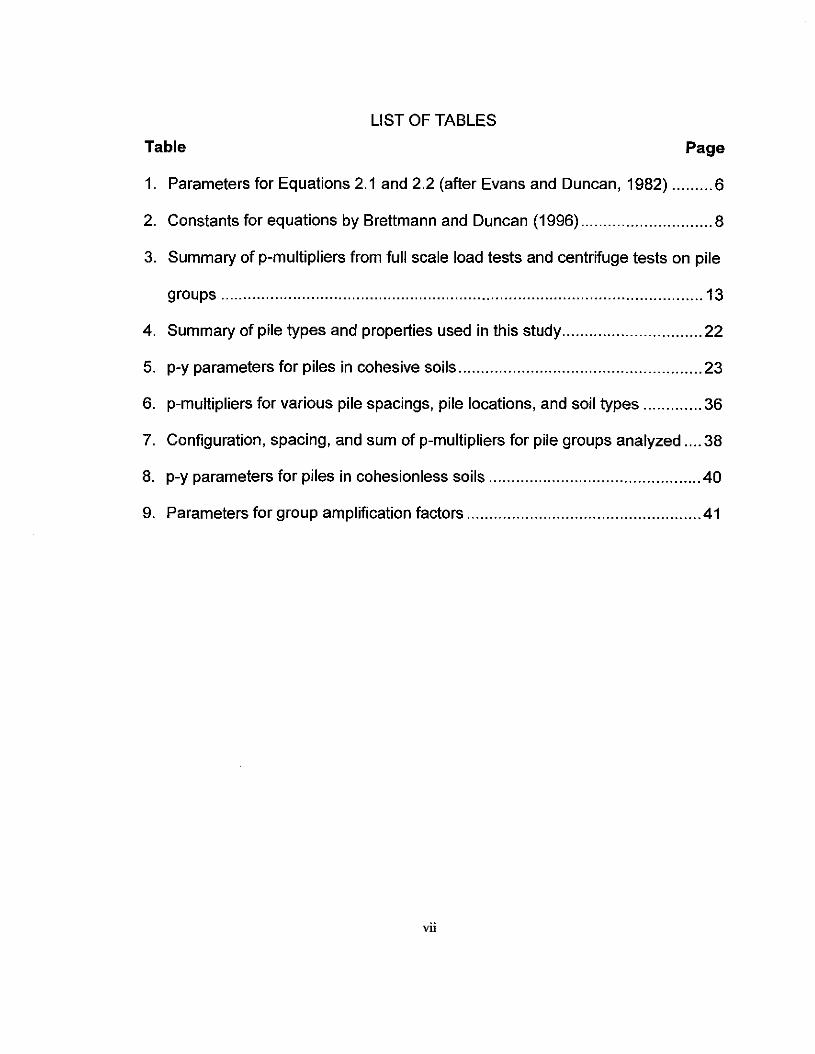
LIST OF TABLES

Table Page

1. Parameters for Equations 2.1 and 2.2 (after Evans and Duncan, 1982) 6

2. Constants for equations by Brettmann and Duncan (1996) 8

3. Summary of p-multipliers from full scale load tests and centrifuge tests on pile

groups 13

4. Summary of pile types and properties used in this study 22

5. p-y parameters for piles in cohesive soils 23

6. p-multipliers for various pile spacings, pile locations, and soil types 36

7. Configuration, spacing, and sum of p-multipliers for pile groups analyzed 38

8. p-y parameters for piles in cohesionless soils .40

9. Parameters for group amplification factors 41

VB

Figure

LIST OF FIGURES

Page

1. Dimensionless load-deflection curves for fixed head piles in sand with zeroembedment. 3

2. Dimensionless load-moment curves for fixed head piles in sand with zeroembedment. 3

3. Dimensionless load-deflection curves for fixed head piles in clay with zeroembedment. 4

4. Dimensionless load-moment curves for fixed head piles in clay with zeroembedment. 4

5. p-mUltiplier concept (Brown et aI., 1988) 12

6. p-multiplier as a function of pile spacing for leading and first trailing row (afterMokwa and Duncan, 2001) 14

7. p-multiplier as a function of pile spacing for the second and third trailing rows(after Mokwa and Duncan, 2001) 15

8. Brown and Bollman's (1993) method (after Hannigan et aI., 1997) 17

9. Dimensionless load-deflection LPILE Plus data points for piles in cohesivesoils with zero embedment 25

10. Dimensionless load-deflection LPILE Plus data points for piles embedded 2,4, 6 and 10ft in cohesive soils 25

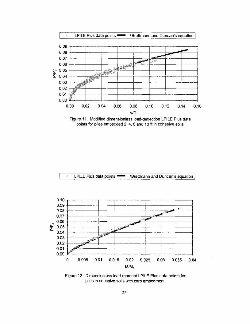
11. Modified dimensionless load-deflection LPILE Plus data points for pilesembedded 2, 4, 6 and 10 ft in cohesive soils 27

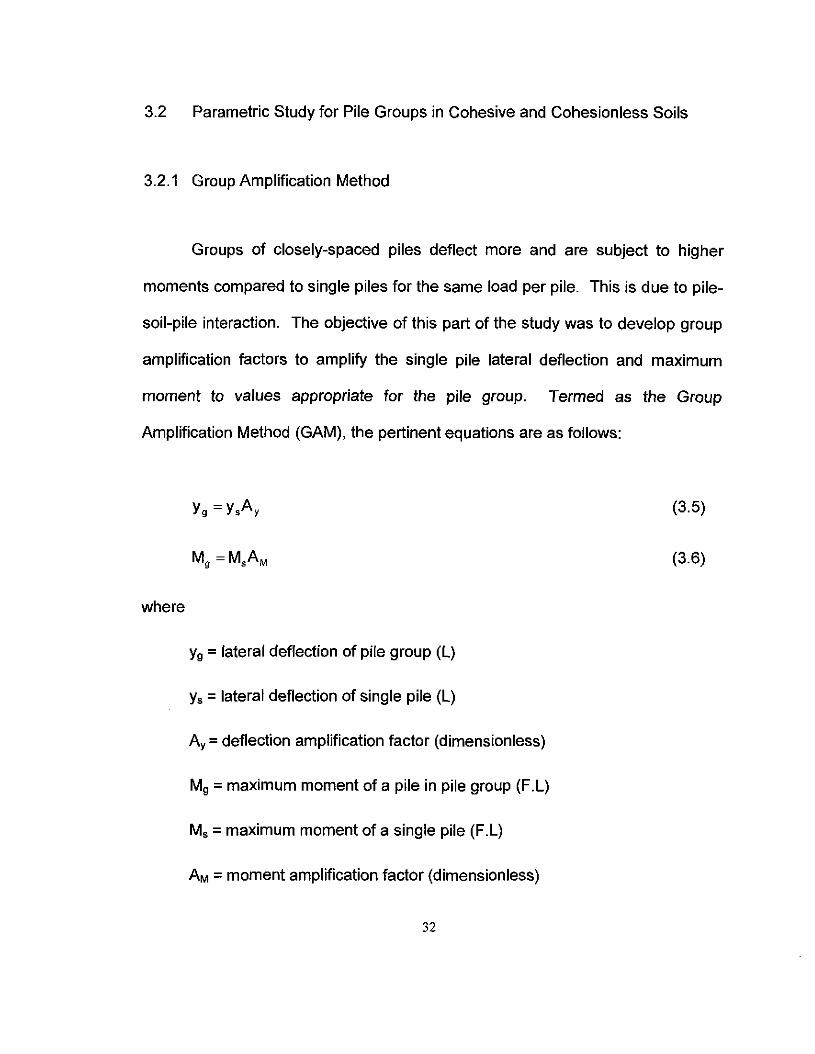
12. Dimensionless load-moment LPILE Plus data points for piles in cohesive soilswith zero embedment 27

13. Dimensionless load-moment LPILE Plus data points for piles embedded 2, 4,6 and 10ft in cohesive soils 29

14. Modified dimensionless load-moment LPILE Plus data points for pilesembedded 2, 4, 6 and 10 ft in cohesive soils 29

viii

15. Comparison of load versus deflection using GEP and GROUP for a R5C5S3group of 48-inch-diameter drilJed shafts with zero embedment in soft clay withSu=0.5ksf 34

16. Comparison of load versus deflection using GEP and GROUP for R3C2S3group of 48-inch-diameter drilled shafts embedded 4 feet in loose sand with III=30° 34

17. Comparison of load versus maximum moment using GEP and GROUP for aR5C5S3 group of 48-inch-diameter drilled shafts with zero embedment in softclay with Su=0.5ksf.. 35

18. Comparison of load versus maximum moment using GEP and GROUP for aR3C2S3 group of 48-inch-diameter drilled shafts embedded 4 feet in loosesand with III =30° 35

19. Pile Configuration in a R3C2S4 pile group 39

20. Comparison of group deflections using GAM versus GEP for piles in cohesive~~ ..........................................................•................................................•...~

21. Comparison of group moment using GAM versus GEP for piles in cohesivewi~ ~

22. Comparison of group deflections using GAM versus GEP for piles incohesionless soils 43

23. Comparison of group moment using GAM versus GEP for piles incohesionless soils 43

24. Pile test layout for case study 1 (a) plan view, (b) and cross-section (Rollinsand Sparks, 2002) 48

25. Comparison of measured versus predicted deflections using GAM for casestudy 1 48

26. Comparison of predicted versus measured bending moments for the SaltLake City load test 50

27. Pile test layout for case study 2 (Kim and Brungraber, 1976) 51


29. Comparison of predicted versus measured bending moment for BucknellUniversity load test 53

ix

30. Pile test layout for case study 3 (Huang et aI., 2001) 55


x

CHAPTER 1

INTRODUCTION

Most structures are subject to latera/loads as a result of wind, earthquake,

impact, waves and lateral earth pressure. If these structures are supported on

deep foundations, the foundations have to be designed for lateral loads.

Laterally loaded single piles and pile groups should be designed to be safe

against geotechnical failure, structural failure and excessive deflections. In

general, geotechnical failure seldom governs the design for laterally loaded piles

that are long with respect to its diameter or width. Therefore, this study will focus

on the analyses of laterally loaded piles for deflections and structural failure.

This report describes the research on developing a simplified method to

analyze fixed-head single piles and pile groups subjected to lateral loads. In

Chapter 2, a literature review of current state-of-the-art methods for lateral load

analyses of single piles and pile groups is presented. A description of the

simplified procedures developed in this study to analyze a single and a group of

fixed head piles is presented in Chapter 3. In Chapter 4, three full-scale lateral

load tests on groups of fixed-head piles are evaluated where the predicted

responses are compared with measured results.

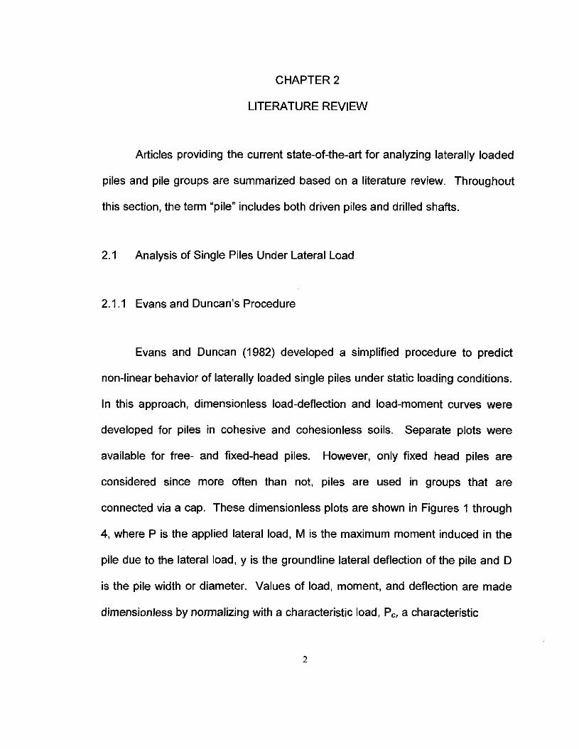
CHAPTER 2

LITERATURE REVIEW

Articles providing the current state-of-the-art for analyzing laterally loaded

piles and pile groups are summarized based on a literature review. Throughout

this section, the term "pile" includes both driven piles and drilled shafts.

2.1 Analysis of Single Piles Under Lateral Load

2.1.1 Evans and Duncan's Procedure

Evans and Duncan (1982) developed a simplified procedure to predict

non-linear behavior of laterally loaded single piles under static loading conditions.

In this approach, dimensionless load-deflection and load-moment curves were

developed for piles in cohesive and cohesionless soils. Separate plots were

available for free- and fixed-head piles. However, only fixed head piles are

considered since more often than not, piles are used in groups that are

connected via a cap. These dimensionless plots are shown in Figures 1 through

4, where P is the applied lateral load, M is the maximum moment induced in the

pile due to the lateral load, y is the groundline lateral deflection of the pile and D

is the pile width or diameter. Values of load, moment, and deflection are made

dimensionless by normalizing with a characteristic load, Pc, a characteristic

2

Evans and Duncan's range (1982)

Brettmann and Duncan's equation (1996)

0.0350.005 0.01 0.015 0.02 0.025 0.03

ylDFigure 1. Dimensionless load-deflection curves

for fixed head piles in sand with zero embedment

j --~~~

.........-......I ...,....,~

A-~9

~.;f/',

i I

0.01

oo

0.014

0.012

0.004

0.002

" 0.008a-

c: 0.006

I

i Evans and Duncan's range (1982)--]

- - - -Brettmann and Duncan's equationJ.1~96)

---------+------1

0.014

0.012

0.01

" 0.008a--a- 0.006

0.004

0.002

00 0,002 0.004 0.006 0.008 0.01

MIMe

Figure 2. Dimensionless load-moment curvesfor fixed head piles in sand with zero embedment

3


Brettmann and Duncan's equation (1996)

!

i-, ----- ~

~~-:- c··· .-

~~

/ "'",

~. . -I.

e i

0.06

0.05

0.04

<Ja- 0.03c:

002

0.01

o0.00 0.01 0.02 0.03 0.04 0.05 0.06 0.07

Figure 3. Dimensionless lo~~~eflectlon curvesfor fixed head piles in clay with zero embedment


- - - .Brettmann and Duncan's equation (1996)

0.06

0.05

0.04

0a- 0.03-a-

0.02·

0.01

0

0 0.005 0.01 0.015 0.02 0.025

MIMeFigure 4. Dimensionless load-moment curves

for fixed head piles in clay with zero embedment

4

moment, Me, and the pile width or diameter, 0, respectively. Pc and Me are

expressed as follows:

(2.1 )

(2.2) .

where

o =pile width or diameter (L)

E =Young's modulus of the pile (FL-2)

R1 = moment of inertia ratio (dimensionless)

IRJ =

I,

I = moment of inertia of the pile (L4)

I, =moment of inertia of a solid circular cross section of diameter 0 (L4)

nO'1=, 64

(2.3)

(2.4)

The remaining parameters for the equations are summarized in Table 1.

The behavior of the pile under lateral load is governed by the soil within the top

eight pile diameters. The moist and buoyant unit weights of the soil should be

used above and below the water table, respectively. The Evans and Duncan

(1982) procedure only applies to piles where the top is at the ground surface.

5

Table 1. Parameters for Equations 2.1 and 2.2 (after Evans and Duncan, 1982)

Parameters Sands Clay

Pc Mc Pc Mc

F= dimensionless 1 1 1 for plastic 1 for plasticparameter related to clay claystress-strain behavior ofthe soil 1.54 for 1.343 for

brittle clay brittle clay

m= passive pressure 0.57 0.40 0.683 0.46exponent

n= strain exponent -0.22 -0.15 -0.22 -0.15

up= representative up = 2CP4>yD tan2(45°+~/2) Up = Cpc Supassive pressure of soil(FL-2) Cp~ = dimensionless Cpc = dimensionless

modifying factor to modifying factor toaccount for three- account for three-dimensional effect of the dimensional effect of thepassive wedge in front of passive wedge in front ofthe pile = ~/1 0 the pile and found to be

4.2 for cohesive soils in$=internal friction angle their studyof the soil (degrees)

y= unit weight of soil

E50= strain at which 50% E50= 0.002 for sands E50 ranges from 0.004 toof the strength of the soil 0.020 for plastic claysis mobilized

6

2.1.2 Characteristic load Method (ClM)

The characteristic load method (Duncan et aI., 1994) is a modification of

the Evans and Duncan procedure, where the equations for Pc and Me are

simplified as shown in Equations (2.5) through (2.8):

For sand

For sand

For clay

For clay

P = 1.57D2fER {Y'Dlj)'tan2(45" + lj)/2)JO.

57

c ~ I ERI

M =1.33D3(ER {Y'Dlj)'tan2(45' +lj)/2)jO.40

c I ERI

P = 7.34D 2 (ER {~jO.68c ~ I ER

I

M = 3.8603(ER {~j0.46c I ER

I

(2.5)

(2.6)

(2.7)

(2.8)

The parameters have been defined in Section 2.1.1.

2.1.3 Brettmann and Duncan's Equations

Brettmann and Duncan (1996) developed exponential equations for the

dimensionless nonlinear relationships between load-displacement and load-

moment as shown in Figures 1 through 4. The equations are as follows:

7

(y/D) = a (PIPdb

(MIMe) =c (PIPO)d

where a, b, c and d are summarized in Table 2.

(2.9)

(2.10)

Table 2. Constants for Equations by Brettmann and Duncan (1996)

Constant Fixed-Head Piles in Sand Fixed-Head Piles in Clay

a 28.8 14.0

b 1.5 1.846

c 2.64 0.78

d 1.3 1.249

2.1.4 LPILE Plus 3.0 for Windows

LPILE Plus 3.0 for Windows (Reese and Wang, 1997) is commercial

software that can be used to analyze the behavior of a single pile under lateral

load. The program uses a finite difference technique to estimate deflection,

shear, bending moment, and soil reaction varying with depth. Soil behavior is

modeled using a series of discrete non-linear springs. The stiffnesses of these

springs are characterized using p-y curves, which can be user-defined or

internally generated by the computer program following published

recommendations for various types of soils. These p-y curves were developed

based on results of full-scale lateral load tests on piles in a variety of soils and

8

loading conditions. A wide variation of pile-head boundary conditions may be

selected in the program. The properties of the pile can also vary as a function of

depth. The program also has the capability of considering the non-linear

behavior of concrete piles as a result of cracking.

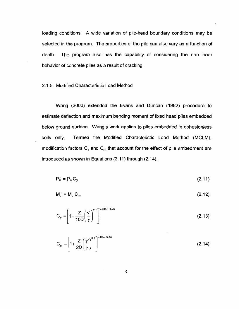
2.1.5 Modified Characteristic Load Method

Wang (2000) extended the Evans and Duncan (1982) procedure to

estimate deflection and maximum bending moment of fixed head piles embedded

below ground surface. Wang's work applies to piles embedded in cohesionless

soils only. Termed the Modified Characteristic Load Method (MCLM),

modification factors Cy and Cm that account for the effect of pile embedment are

introduced as shown in Equations (2.11) through (2.14).

Me' = Me Cm

[

01]0.0850-1.05

Z ( ').C = 1+- Ly 10D y

[

01]0.030-0.65

Z ( ').C = 1+- Lm 20 y

9

(2.11 )

(2.12)

(2.13)

(2.14)

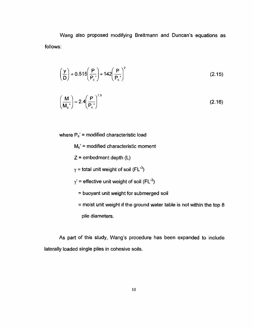
Wang also proposed modifying Brettmann and Duncan's equations as

follows:

(2.15)

(2.16)

where Pe' = modified characteristic load

Me' = modified characteristic moment

Z =embedment depth (l)

y = total unit weight of soil (Fl-3)

y' =effective unit weight of soil (Fl-3)

= buoyant unit weight for submerged soil

=moist unit weight if the ground water table is not within the top 8

pile diameters.

As part of this study. Wang's procedure has been expanded to include

laterally loaded single piles in cohesive soils.

10

2.2 Analysis of Pile Groups Under Lateral Load

Pile groups can be divided into two categories:

1. widely spaced piles which interact only through the pile cap

connection. In these piles, the group response can be estimated by

summing the individual pile responses.

2. closely spaced piles are defined as those in which the response of an

individual pile is influenced through the adjacent soil by the response

of other nearby piles. This "shadowing" effect is commonly termed

pile-soii-pile interaction.

This study deals primarily with closely spaced piles, which involves the

majority of pile groups in practice.

2.2.1 The Concept of p-multipliers

For a group of closely-spaced piles, pile-soil-pile interaction can be taken

into account by introducing reduction factors to the soil reaction (p) portion of the

p-y curves for single piles as shown in Figure 5 (Brown et aI., 1988). These p

multipliers are typically less than or equal to one. They have been

experimentally derived either from full-scale load tests or from tests in a

11

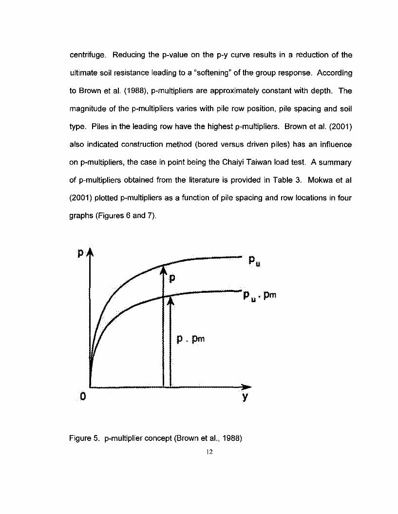
centrifuge. Reducing the p-value on the p-y curve results in a reduction of the

ultimate soil resistance leading to a "softening" of the group response. According

to Brown et al. (1988), p-multipliers are approximately constant with depth. The

magnitude of the p-multipliers varies with pile row position, pile spacing and soil

type. Piles in the leading row have the highest p-multipliers. Brown et al. (2001)

also indicated construction method (bored versus driven piles) has an influence

on p-multipliers, the case in point being the Chaiyi Taiwan load test. A summary

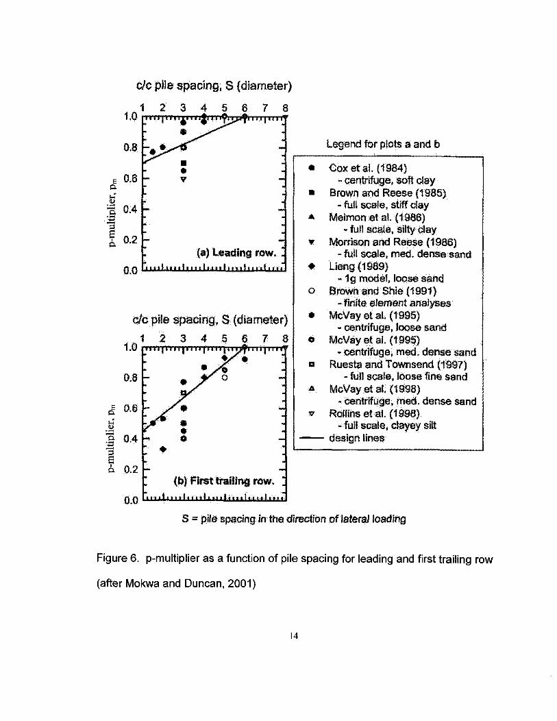
of p-multipliers obtained from the literature is provided in Table 3. Mokwa et al

(2001) plotted p-multipliers as a function of pile spacing and row locations in four

graphs (Figures 6 and 7).

p

.-I...r-----pu ' pm

p .pm

o

Figure 5. p-multiplier concept (Brown et ai., 1988)

12

y

Table 3. Summary of p-multipliers from full scale load tests and centrifuge tests on pile groups

location Te" Size PHe Type Center- Pile Soil Sh.... DefleCtjon ulti lier ReferenceType of to Fixity Type strength 1st Row 2nd Row 3rd Row 4th Row 5th Row 6th Row 7th Row

Pile Center at Top ParameterGroups Spacing (Inches)

Brittany,Steel H-Pile (d=11.2",bf=10.6',) with Meimon et aI.,

Full-scale 3X2 Side Plates welded to Fonn a Box 3D Free-head Clay Su -420 pSf 0.0 0.0 0.5 . · · 1986France

Section

10.75" 00 Steel Pipe Pile with Wall 1.2 0.7 0.0 0.5 · · Brown et al.,Houston, TX Full-scale 3X3

Thickness = 0.365" & Grout Fill3D Free-head Clay Su ~ 1500 psf 1967

2.0 0.7 0.5 0.0 · ·Salt lake City, 12" 00 Steel Pipe Pile with

Rollins et aI.,Full-scale 3X3 3D Free-head Clay Su ~ 1000 psf 1.0to2.4 0.0 0.0 0.0 · · 1990

UT Concrete Fill

Salt lake City, 12" 00 Steel Pipe PUe withSparks &

Full-scale 3X 3 3D Fixed-head Clay Similar to Free-Head According to Rollins et al., 1998 Rollins, 1997UT Concrete Fill

10.75" OD Steel Pipe Pile with Wall 0- 38" Brown et al.,Houston, TX Full-scale 3x3

Thickness = 0.365" & Grout Fill3D Free-head Sand 1.0to 1.5 0.0 0.0 0.3 · · 1988

Dr> 90%

Brown et al.,2x3 1.5-m Drilled Shaft 3D Fixed-head 1.2 0.5 0.0 0.3 · · 2001

Chaiyi, Taiwan Full-scale Sand 0=35"

3XOO.8-m 00 Prestressed Concrete 3D Fixed-head 0.0 0.0 0.7 0.5 0.0 ·• Pile ·

)

30"X30" Square PrestressedRuesta &

Stuart, FL Full-scale OXOConcrete Piles

3D Free-head Sand 0=32" 1.0to3.0 0.8 0.7 0.3 0.3 · . Townsend,1997

· Centrifuge 3X3 16.9" 00 Pipe P'.e (42.7 fllong) 3D Free-head Sand Dr =-33% · 0.65 0.45 0.35 · · McVayet at,1995& Pinto

· Centrifuge 3X3 16.9" 00 Pipe Pile (42.7 fllong) 5D Free-head Sand Dr =33% · 1 0.85 0.7 · etal.,1997

· Centrifuge 3X3 16.9" 00 Pipe Pile (42.7 fllong) 3D Free-head Sand Dr = 55% · 0.8 0.0 0.3 · ·

· Centrifuge 3X3 16.9" 00 Pipe Pile (42.7 ft long) 5D Free-head Sand Dr= 55% 1 0.85 0.7 · ·

Centrifuge 3X3 16.9" 00 Pipe Pile (45 ft long) 3D Free-head Sand Dr=36&55% · 0.8 0.0 0.3 · McVayetal.,1998

Centrifuge 3XO 16.9" 00 Pipe Pile (45 fl long) 3D Free-head Sand Dr=36&55% 0.8 0.0 0.3 0.3 · ·

Cenlrifllge 3X5 16.9" DO Pipe Pile (45 ft long} 3D Free-head Sand Dr=36&55% 0.8 0.0 0.3 0.2 0.3 · .

Centrifuge 3X6 16.9" 00 Pipe Pile (45 fllong) 3D Free-head Sand Dr= 36 &55% 0.8 0.0 0.3 0.2 0.2 0.3

Centrifuge 3X7 16.9" OD Pipe Pile (45 f1long) 3D Free-head Sand Dr=36&55% 0.8 0.0 0.3 0.2 0.2 0.2 0.3

~

'"

a The first number refers to the number of plies in each row. The second number refers to the number of rows of piles in the group.

crc pile spacing, S (diameter)

1 234 5 6 7 81.0 I'1TMl'l"1T1rrrn-ntr~'m;ol""""'l'l"1T1n"1'

Legend fOT PlOts a and b

• Cox et at (1984)• centrifuge,soft clay

• BroWn and Reese (1985)• fun scale, stiff clay

.. Melmonetal.(t986)• full scale, silty clay

... Morrison and Reese (19SB)-full scale, mad. dense sand

• Lieng (1989)• 19 model, loose sand

o arowhand Shie (1991)- finite element analyses

• McVay etal. (l995)• centrifuge. loose sand

o McVay etal. (11'195)• oontrifug~.• med. dense sand

II Ruesta and Townsend (1997)- full scale,loosilfine sand

.0. McVayet al. (1998)• ool1lrif4ge. med. dense $and

v Rollins etal. (1998)• full scale. clayey silt

- desigl1lines

(a) Leading row.

•

c!cpile spacing, S(diameter)

1 234 5 6 7 81.0 .

0.8

J 0.6

0.8

••E 0.6 v

l:>-

~.~ 0.4-l:>-.~

.~0.2,

l:>-

0.0

(b) Firstfraiflng row.0.0 LLU.LWu.u.................u.u.I..I..I.L.L.U.Iu.u.LL1

S = pile spacingintha direction oflstera//oadlng

Figure 6. p-multiplier as a function of pile spacing for leading and first trailing row

(after Mokwa and Duncan. 2001)

14

cJc pile sp$oing,S (diameter)

123456781.0 1TT't"rm-,..,.,.,..,,..,.,.,..,.,.,.,.,'TTT"CI"T'I'TMTl"1,"

(a) Seeomf trailing row.

Legend for plots a .and b

• Cox etaL (1984)-centrifuge. soft clay

• Brown and Reese>(1985)" fuU scale, stiff clay

... Morrison and Reese (1986)- fUll scale, med. densesahd

•• McVay at a.l. (1995)-centrifuge, [oosesand

o McVayet at. (1995)-centrifuge. mad.. dense sand

II Ruesta andTClWnsend (1997)- full scale,. loose fine sand

A McVayet al. (1998)- centrifuge, med. dense sand

v RoUlnsl'lt al. (1998)• fullscale, clayey silt

- design lines

o

•

•

(b) 3rd and greatertrailing rows,

etc pile spacing, S(diameter}

1 234 5 6 7 81.0 ITTTTTMT1T1TlT1I'1TT'1.......rllITl"'ITTl'TTI1

0.8

0.2

0.8E~

l"i 0.6.~-.S-

~ 0.4,~

0.2

J• 0.6Ii)

:.::::i 0.4,~

Figure 7. p-multiplier as a function of pile spacing for the second and third

trailing rows (after Mokwa and Duncan, 2001)

15

2.2.2 Brown and Bollman's Method

Brown and Bollman (1993) developed a procedure to analyze the behavior

of pile groups under lateral load by performing separate p-y analysis for each row

using appropriate values of p-multipliers for each row. The series of p-y analyses

is set up as follows for symmetric pile groups:

1. Determine the p-multiplier for each row according to row position, pile

spacing, and soil type.

2. Perform p-y analyses for one pile in each row using the appropriate p

multiplier for that row.

3. Plot the lateral load versus deflection for the pile analyzed in each row (see

Figure 8). The lateral load per pile-deflection curve of the pile group can be

estimated by summing the lateral loads for the pile in each row at the same

lateral deflection and diViding this sum by the number of rows.

4. The maximum bending moment in the most heavily loaded pile in the group

corresponds to the bending moment in the piles in the leading row.

16

600 Front Row

LoadPer Pile

Lateral Load IPer Pile, (kN)400 3rd - 4th Rows

200Estimated Pile

---- Group Deflection

a}a 25 50 75

150

Pile Head Deflection (mm)

Estimated Pile_.....--- Group Deflection

Front Row

2nd Row3rd - 4th Rows

Maximum

Bending Moment

Per Pile, (kN-m)

b}

100

50

a 25 50 75

Pile Head Deflection (mm)

Figure 8. Brown and Bollman's (1993) method (after Hannigan et aI., 1997)

17

2.2.3 Mokwa and Duncan Group Equivalent Pile Procedure

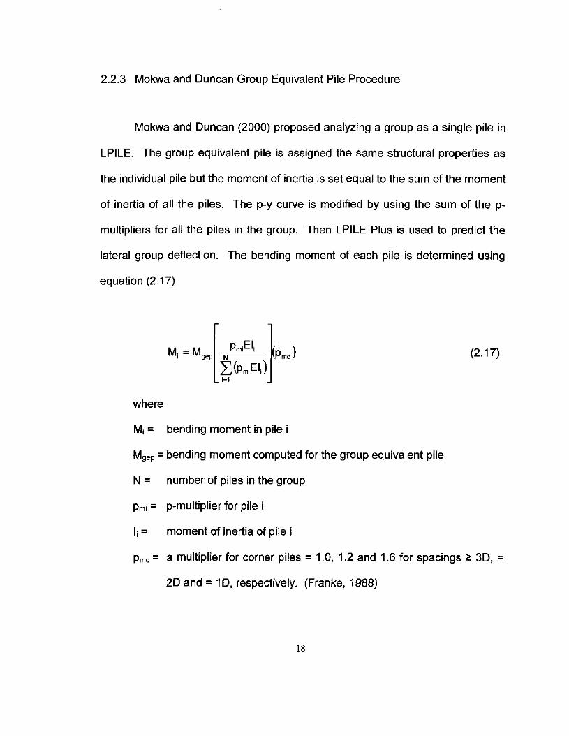
Mokwa and Duncan (2000) proposed analyzing a group as a single pile in

LPILE. The group equivalent pile is assigned the same structural properties as

the individual pile but the moment of inertia is set equal to the sum of the moment

of inertia of all the piles. The p-y curve is modified by using the sum of the p-

multipliers for all the piles in the group. Then LPILE Plus is used to predict the

lateral group deflection. The bending moment of each pile is determined using

equation (2.17)

where

M; = bending moment in pile i

Mgep = bending moment computed for the group equivalent pile

N = number of piles in the group

Pm; = p-multiplier for pile i

I; = moment of inertia of pile i

(2.17)

Pmc = a multiplier for corner piles = 1.0, 1.2 and 1.6 for spacings ~ 3D, =

20 and::: 10, respectively. (Franke, 1988)

18

2.2.4 GROUP 4.0 for Windows and FBPier

Two state-of-the-art computer programs with the capability for analyzing

pile groups are reviewed in this section. GROUP for Windows (Reese and

Wang, 1996) is a commercial program for analyzing groups of vertical or battered

piles. Moment, lateral loads or a combination of the two may be applied to the

group. Possible options of connectivity to the pile cap include fixed, pinned, or

elastically restrained. The program solves by iteration for the nonlinear response

of each pile under combined loading, and checks for compatibility of geometry

and equilibrium of forces between the applied external loads and the reactions of

each pile head. The load-deflection and load-moment relationships for each pile

in its individual coordinate system are computed by solving nonlinear differential

equations using p-y and t-z curves under lateral and axial loading, respectively.

For closely-spaced piles, the pile-soil-pile interaction can be taken into account

by introducing reduction factors for the p-y curves used for each single pile. The

program can compute the deflection, bending moment, shear, and soil resistance

as a function of depth for each pile.

FBPier (Bridge Software Institute, 2003) is a more sophisticated non-

linear, finite element analysis, soil-structure interaction program developed at the

University of Florida. The program can be used to perform a complete

substructure design considering both the geotechnical and structural aspects.

The program can be used to analyze single piles, pile groups, pile bents,19

retaining walls, and high mast lighting structures. Analysis capabilities include

combined axial, lateral, and rotation resistance of the piles, pile cap and pier.

The structural model includes both linear and non-linear (concrete cracking, steel

yielding) capabilities, as well as biaxial interaction diagrams for all sections. It

also allows the use of different pile types within a group.

2.3 Limitation of the Procedures Described

The Evans and Duncan procedure and the ClM cannot be used to predict

the lateral behavior of single piles embedded below the ground surface. The

MClM can account for pile head embedment but to date, it has only been

developed for single piles in cohesionless soils. In this study, the MClM is

developed for single piles in cohesive soils. A new simple technique is also

developed to analyze the behavior of pile groups based on the concept of p

multipliers and using the GEP method. This procedure is simple enough that it

can be readily performed in a spreadsheet or using a calculator.

20

CHAPTER 3

DEVELOPMENT OF SIMPLIFIED PROCEDURE FOR ANALYSIS OF

LATERALLY LOADED SINGLE PILES AND PILE GROUPS

3.1 Parametric Study for Single Piles in Cohesive Soils

LPILE Plus 3.0 for Windows was used to perform a parametric study on

the response of laterally loaded fixed-head piles in saturated cohesive soils with

different embedment depths. The study included three hundred analyses

generating about 1,700 load cases. The main parameters considered include

pile type, pile size, undrained shear strength, and embedment depth. A range of

lateral loads was applied to the top of the piles to obtain load-deflection and load-

moment curves.

Analyses were conducted on both driven piles and drilled shafts. Driven

piles analyzed included steel pipe piles, steel H-piles, and precast prestressed

concrete piles. Detail properties of the piles used in the parametric study are

shown in Table 4. Pile diameters or widths analyzed were between 9.7 inches

and 48 inches. The flexural stiffness of the piles ranged from 3.31 x 106

to 9.38 X 108 kip-in2. When the pile extreme fiber stresses exceeded the

allowable values, the pile failed structurally. These load cases are not included

in the parametric study.

21

Table 4. Summary of pile types and properties used in this study

Pile Type Pile Description Pile Width or Area E" Ib

Diameter(inches) (in') (ksi) (in4

)

Steel H-pile HP10x42 9.7 12.40 29000 210

Steel H-pile HP12x74 12.13 21.80 29000 569

Steel H-pile HP14x102 14.01 30.00 29000 1050

Steel Pipe Pile 10o/.-inch-diameter 10.75 8.25 29000 114Y..-inch-thick wall

Steel Pipe Pile 12o/.-inch-diameter 12.75 14.60 29000 279318-inch-thick wall

Steel Pipe Pile 14-inch-diameter 14 16.10 29000 3733/8-inch-thick wall

Precast Prestressed 14-inch-square 14 196.00 4300 3201Concrete Pile f,"=5000psi

Precast Prestressed 14-inch-square 16 256.00 4300 5461Concrete Pile f,'=5000psi

Drilled Shaft 18-inch-diameter 18 254.47 3600 5153f,'=4000psi




a E = Young's modulus of pile

b I = moment of inertia of pile

e fe' = 28-day compressive strength of concrete

22

Four values of undrained shear strength (0.5, 1, 2 and 4 ksf) were assumed.

Matlock's (1970) soft clay model was used for cohesive soils with undrained

shear strengths of 0.5 and 1 ksf while Reese and Welch's (1975) stiff cohesive

soil model was used for undrained shear strengths of 1, 2 and 4 ksf. p-y

parameters for the soils are summarized in Table 5. Both models were used to

analyze cohesive soils with an undrained shear strength of 1 ksf to observe any

differences between the two models. A comparison of the two models showed

no major differences when analyzing cohesive soils with an undrained shear

strength of 1 ksf

Table 5. p-y parameters for piles in cohesive soils

Soil model Undrained shear strength Soil modulus £50(ksf) (pci)

Soft clay 0.5 0 0.02

Soft clay 1 500 0.01

Stiff clay 1 500 0.007

Stiff clay 2 1000 0.005

Stiff clay 4 2000 0.004

The pile top was embedded at several depths below ground surface.

Embedment depths considered include 0, 2,4,6 and 10 feet.

23

3.1.1 Modified Characteristic load for Single Piles in Cohesive Soils

Initially, lPllE analyses were performed for piles with zero embedment to

confirm that the analyses yielded results that are consistent with Brettmann and

Duncan's (1994) equation. The results plotted in Figure 9 show good agreement.

The analyses were then extended to include piles with non-zero embedment and

the results are presented in Figure 10. Evans and Duncan's characteristic load

for the case of zero-embedment was used to normalize the lateral load. The

figure shows wide scatter, and the Evans and Duncan procedure tends to

overestimate deflection. Thus, as embedment depth increases, the deflection

decreases under the same lateral load indicating that the increase in lateral earth

pressure significantly influences the lateral behavior of piles.

To make the ClM applicable to the cases with non-zero embedment

depth, the equation for the characteristic load must be modified so that the

calculated load-deflection points all fall on the Evans and Duncan trend line. An

embedment correction factor Cy was developed for the characteristic load (Pc) to

obtain a better match between the lPllE results and the Evans and Duncan

procedure. The correction factor is applied to the characteristic load as follows:

24

LPILE Plus data points - 'Bretlmann and Duncan's equation I

0.160.140.120.100.060.040.02 0.08

y/DFigure 9. Dimensionless load-deflection LPILE Plus data points for

piles in cohesive soils with zero embedment

0.10 r----,--,----r--,--.........,.--,---,--,

0.00 "_0.08 -- .. ,.D' ...~

o ~.~~ ~••~;iJ~'--'=---;--1---'-f----+-------1a: 0.05 {f :+14'~-C,d"'~t~Qi_,_-,.,F---+----+----+---+-----j

0.04 __.:lw~'0.03 -~~~r._---- ._--+---+--+---+----1----+----10.02 tif0.01 r'---t---t---+--+---+---t---t----I0.00 -J----j---t---+----j---t----j-----I----J

0.00

~. - LPILE Plus data points - 'Bretlmann and Duncan's equation I

0.160.140.120.100.04 0.06 0.08

y/D

Figure 10. Dimensionless load-deflection LPILE Plus data points forpiles embedded 2, 4, 6 and 10 It in cohesive soils

0.12

0.10

0.08

0!l- 0.06-!l-

0.04

0.02

0.00

0.00 0.02

25

( )(~+0"5JZ 1000yD

C = 1+-y 0

where

Pc' =modified characteristic load (F)

o = pile diameter or width (L)

Z = embedment depth of pile top below ground surface (L)

y =effective unit weight of soil over top 80 (FL'3)

= buoyant unit weight for submerged soil

= moist unit weight for soils above the ground water table

Su = undrained shear strength (FL'2)

(3.1 )

(3.2)

Cy equals one when the embedment depth is zero, is greater than 1.0 for

positive embedment and is not applicable for piles extended above ground.

When the modified characteristic load is used to normalize the lateral load, the

revised dimensionless load-defection points all fall within a narrow range close to

the Brettmann and Duncan curve as shown in Figure 11.

26

o LPILE Plus data points - 'Brettm~mn:;;~d Duncan's eq~~n]

0.160.140.12

----]---- ---_._-

0.100.060.040.02 0.08

ylD

Figure 11. Modified dimensionless load-<leflection LPILE Plus datapoints for piles embedded 2, 4, 6 and 10 It in cohesive soils

0.09 ~'-"""""---'---,---r---r---,--~----,0.08 +--+----f--+-----+-------i-._-",""--±!"""';;;;;;:....-"'1"""==-----10.07 ~~o••

0.06 !==~==!:;~~~~-.~-;,------:-·~-=·--·t···=·=·~~~~-=-=-=-1I--=--=--=--=jcL 005 +---t--~

c:: 0.04

0.03

002

0.010.00 'iI---+---I----I-----!---j.---I------I--__I

0.00

LPILE Plus data points - _'Breltl11ann and Duncan's equation I

0040.03 0-0350.0250.02

MIMe

0.0150.010.005

0.10 .,.----,----,----,.-----,-------,.--,--.........,--..,:

0.09 +----+--- i ,00.08 +-_--+__-+-__+-_--+__ ..J, . -" -ii~' f-

0.07 +---+----+--+----+--_-4'-+d;~=.,.,"'"""'F--+------10.06 +----+-- -----+--_____j~~~C+-------jI----+------j

cL '."",';;"i2-j-"~---+---+----+-----l£i: 0.05 +---+-----t---~-.,f-,"'~;,..,0.04 ~_

0.03 AiiIJfli~--+---+--+---+---+------I

~:~~ .~I---+--+---+--+---+--+----I0.00 -I"---+---I---+---+----I--4----I--.....j

o

Figure 12. Dimensionless load-moment LPILE Plus data points forpiles in cohesive soils with zero embedment

27

3.1.2 Modified Characteristic Moment for Single Piles in Cohesive Soils

Using the LPILE results, dimensionless load-moment curves for zero

embedment are plotted in Figure 12. The lateral load is normalized by the

characteristic load, Pe, while the maximum bending moment is normalized by the

characteristic moment, Me. The LPILE data points all fall within a narrow range

illustrating the reliability of the Evans and Duncan procedure. Again, the

dimensionless load-moment points for non-zero embedment show poor

agreement as seen in Figure 13, where a large scatter can be observed.

A correction factor, Cm, was developed to modify the characteristic

moment, Me, for non-zero embedment depth as follows:

where Me' is the modified characteristic moment.

(Z J(~02)

C = 1+-m 60D

28

(3.4)

(3.3)

LPILE Plus data points - 'Breltmann_llnd Duncan's equation I

0.005 0.01 0.015 0.02 0.025 0.03 0.035 0.04

MIMeFigure 13. Dimensionless load-moment LPILE Plus data points for

piles embedded 2, 4, 6 and 10 fl in cohesive soils

{)

0.12

0.10

0.08

00- 0.06-0-

0.04

0.02

0.000

c; LPILE Plus data points - 'Breltmann and Duncan's equ~ti~ri]

•0.09 ~----r-------c--_-__-_--_----,0.08 -1-----I---L--+----I----l----:-~~--___i

0.07 +----+---+i--+-----1--_l_--:o-~;t,,""';l-_l_------10.06 -l----+------+--+_--f-- A-,&j4'''~''---f---+------1

------1--+----+---+-----1

0.005 0.01 0.015 0.02 0.025 0.03 0.035 0.04

rL 0.05

a: 0.04 -1-----1--_"_

0.03

0.02

0.01

0.00 ~--+--_+_-_+--+_-__I--_+--I__--J

oMIMe'

Figure 14. Modified dimensionless load-moment LPILE Plus datapoints for piles embedded 2, 4, 6 and 10 fl in cohesive soils

29

When the modified characteristic load, Pc' and modified characteristic

moment, Me', are used to normalize the load-moment points for the case of non

zero embedment, the scatter diminishes as shown in Figure 14.

3.1.3 Steps for the Modified Characteristic Load Method

Steps for analyzing the behavior of laterally loaded piles in cohesive soils

using the MCLM are:

1) Calculate the modified characteristic load using Equations (2.1), (3.1), and

(3.2).

2) For a given lateral load, P, calculate the dimensionless lateral load PIPe'.

3) Use Brettmann and Duncan's Equation (2.9) to estimate the dimensionless

deflection YID corresponding to the dimensionless load from Step 2.

4) Calculate the deflection by multiplying the estimated dimensionless deflection

from Step 3 with the pile width or diameter.

5) Calculate the modified characteristic moment using Equations (2.2), (3.3),

and (3.4).

6) Use Brettmann and Duncan's Equation (2.10) to estimate the dimensionless

moment MIMe' corresponding to the value of PIPe' from Step 2.

7) Multiply the dimensionless moment from Step 6 with the modified

characteristic moment from the Step 5 to determine the maximum bending

30

moment M. Since the pile head is fixed, the maximum bending moment

occurs at the top of the pile.

This method has the following limitations.

(1) The MCLM applies only to vertical piles.

(2) This study was performed assuming long piles only which are very common

in practice. This method is not applicable to short piles with low LID ratios.

(3) Cases where the pile failed structurally are not included in the parametric

study.

(4) This method cannot automatically account for nonlinear behavior of

reinforced concrete piles after cracking. However, the engineer may

manually reduce the flexural rigidity of the pile to account for this non-linear

behavior.

(5) The maximum embedment depth involved in this study was 10 feet.

(6) Only static lateral loads were considered in this study.

(7) The method assumes uniform soil properties within the top 8 pile diameters.

For layered systems, the average properties within the top eight pile

diameters should be used.

31

3.2 Parametric Study for Pile Groups in Cohesive and Cohesionless Soils

3.2.1 Group Amplification Method

Groups of closely-spaced piles deflect more and are subject to higher

moments compared to single piles for the same load per pile. This is due to pile

soil-pile interaction. The objective of this part of the study was to develop group

amplification factors to amplify the single pile lateral deflection and maximum

moment to values appropriate for the pile group. Termed as the Group

Amplification Method (GAM), the pertinent equations are as follows:

where

yg = lateral deflection of pile group (L)

Ys = lateral deflection of single pile (L)

Ay =deflection amplification factor (dimensionless)

Mg= maximum moment of a pile in pile group (F.L)

Ms = maximum moment of a single pile (F.L)

AM = moment amplification factor (dimensionless)

32

(3.5)

(3.6)

Amplification factors were developed by running numerous LPILE

analyses to obtain single pile deflections and moments, and by estimating group

deflections and moments using the group equivalent pile (GEP) procedure

(Mokwa and Duncan, 2000). The group amplification factors are then obtained

from the ratio of group response to single pile response. The parametric study

was performed for groups of fixed-head piles in cohesive and cohesionless soils

with different soil parameters, embedment depths, pile arrangements and lateral

load values. The analyses for cohesive and cohesionless soils were studied

separately. When the pile extreme fiber stresses exceeded the allowable values,

the pile failed structurally. These load cases are not included in the parametric

study.

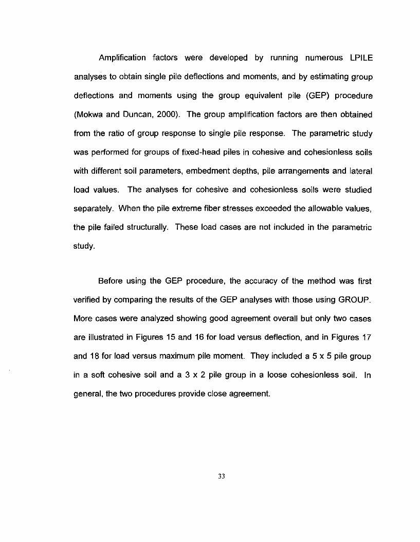
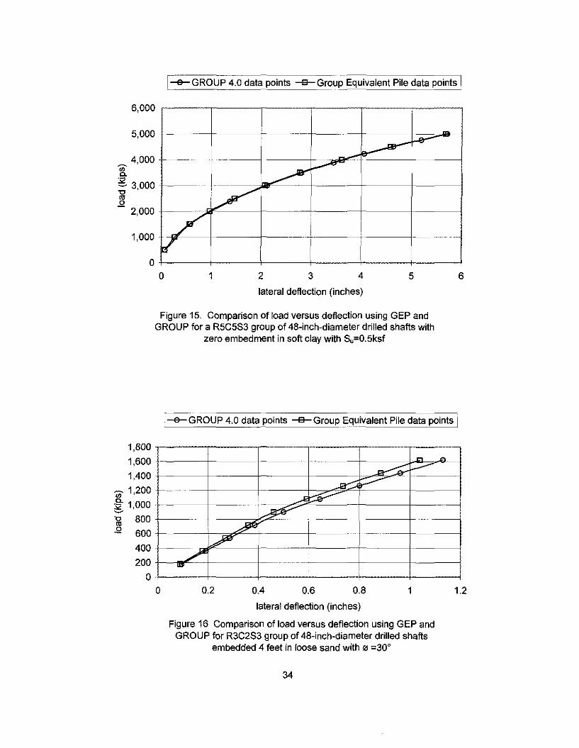
Before using the GEP procedure, the accuracy of the method was first

verified by comparing the results of the GEP analyses with those using GROUP.

More cases were analyzed showing good agreement overall but only two cases

are illustrated in Figures 15 and 16 for load versus deflection, and in Figures 17

and 18 for load versus maximum pile moment. They included a 5 x 5 pile group

in a soft cohesive soil and a 3 x 2 pile group in a loose cohesionless soil. In

general, the two procedures provide close agreement.

33

1_GROUP 4.0 data points -e-Group-Equivaient Pile data points I

-1----I ~,

~---- - --~

~/1 !

~ I.~ -'-',-

6,000

5,000

4,000

\i:g 3,000al.Q

2,000

1,000

oo 1 2 3 4 5 6

lateral deflection (inches)

Figure 15. Comparison of load versus deflection using GEP andGROUP for a R5C5S3 group of 48-inch-diameter drilled shafts with

zero embedment in soft clay with Su=0.5ksf

r=a::GROUP 4.0 data points -e- GroupECluivalent Pile data points!

1.20.8 10.60.40.2

1,800 -r-----r---..,..----,-----,------,----,1,600 +----j----+----- - _.- ----+-----:;~_EI_::~~-"'0>--_1

1,400 -~---------(j) 1,200 c- ---=t===i~~~4~:::=~====~==~~ 1,000 +-----j---~ ~-0 800 +-----\I--~---=~.;...-c----- -------+-----+-----\11 600 +-----+!--'---".:9-~+------+--

400+---/--200 _

oo

lateral deflection (inches)

Figure 16 Comparison of load versus deflection using GEP andGROUP for R3C2S3 group of 48-inch-diameter drilled shafts

embedded 4 feet in loose sand with rIJ =30·

34

I-e-GROUP 4.0 data points Group Equivalent PiI~d~iapomtSJ

I i, -----------..-::::::::-----

~;::;---

..bP- i

.L?V-,,

3500

3000

2500

"'~ 2000~

-g 1500.Q

1000

500

oo 500 1000 1500 2000 2500 3000 3500

maximum moment (ft-kip)

Figure 17. Comparison of load versus maximum moment using GEPand GROUP for a R5C5S3 group of 48-inch-diameter drilled shafts

with zero embedment in soft clay with S,=0.5ksf

I-e-GROUP 4.0 data points ---- Group Equivalent Pile data poi~iS]

3500 -,------,-----r------,-----,----r----,

3000 +----+--- --1---+-------I---+------l

2500 . -_._. ........

600050004000300020001000

~ 2000

~ ::::+---+---+-~--+-~-•......·.•••••-Li-----:-=--4'~=-----j~~

500 t----;;;;~7---1----·~

~

0+----+-----+----+---~--+--____1

omaximum moment (ft-kip)

Figure 18. Comparison of load versus maximum moment usingGEP and GROUP for a R3C2S3 group of 48-inch-diameter drilled

shafts embedded 4 feet in loose sand with r<l =30'

35

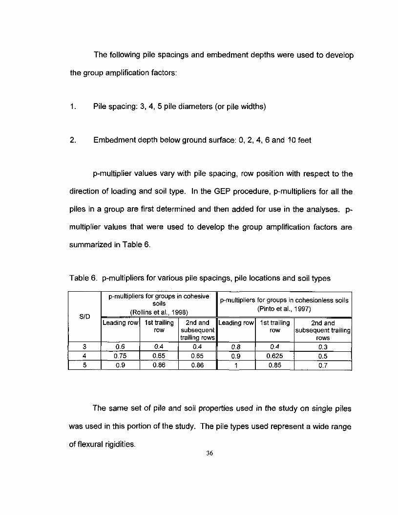
The following pile spacings and embedment depths were used to develop

the group amplification factors:

1. Pile spacing: 3, 4, 5 pile diameters (or pile widths)

2. Embedment depth below ground surface: 0, 2,4,6 and 10 feet

p-multiplier values vary with pile spacing, row position with respect to the

direction of loading and soil type. In the GEP procedure, p-multipliers for all the

piles in a group are first determined and then added for use in the analyses. p-

multiplier values that were used to develop the group amplification factors are

summarized in Table 6.

Table 6. p-multipliers for various pile spacings, pile locations and soil types

p-multipliers for groups in cohesivep-multipliers for groups in cohesionless soilssoils

(Rollinsetal.,1998) (Pinto et aI., 1997)SID

Leading row 1st trailing 2nd and Leading row 1st trailing 2nd androw subsequent row subsequent trailing

trailing rows rows3 0.6 0.4 0.4 0.8 0.4 0.34 0.75 0.65 0.65 0.9 0.625 0.55 0.9 0.86 0.86 1 0.85 0.7

The same set of pile and soil properties used in the study on single piles

was used in this portion of the study. The pile types used represent a wide range

of flexural rigidities.36

A total of 260 GEP analyses were performed to generate 2,200 load cases

for groups in cohesive soils. The pile configuration, pile spacing, and the

corresponding sum of the p-multipliers are summarized in Table 7.

Pile groups are labeled as follows: the first letter "R" indicates the number

of rows, the letter "C" denotes the number of "columns", and the letter "8"

represents the pile spacing in terms of the number of pile diameters. The layout

for pile group R3C284, which consists of 3 rows and 2 columns of piles spaced 4

diameters center-to-center, is shown in Figure 19. A total of eleven group

configurations were analyzed. They include: R1C2, R1C5, R2C1, R2C2, R2C3,

R2C4, R3C2, R3C3, R4C4, R5C1 and, R5C5.

37

Table 7. Configuration, spacing, and sum of p-multipliers for pile groups

analyzed

Group Number Number ofDimensionless

LPm for LPm forPile SpacingDesignation of Rows Columns

(SID) Cohesive Soils Cohesion less Soils

R1C2S3 1 2 3 1.2 1.6

R1C2S4 1 2 4 1.5 1.8R1C2S5 1 2 5 1.8 2

R1C5S3 1 5 3 3 4R1C5S4 1 5 4 3.75 4.5R1C5S5 1 5 5 4.5 5R2C1S3 2 1 3 1 1.2R2C1S4 2 1 4 1.4 1.525R2C1S5 2 1 5 1.76 1.85

R2C2S3 2 2 3 2 2.4R2C2S4 2 2 4 2.8 3.05R2C2S5 2 2 5 3.52 3.7R2C3S3 2 3 3 3 3.6R2C3S4 2 3 4 4.2 4.575R2C3S5 2 3 5 5.28 5.55R2C4S3 2 4 3 4 4.8R2C4S4 2 4 4 5.6 6.1R2C4S5 2 2 5 7.04 7.4R3C2S3 3 2 3 2.8 3R3C2S4 3 2 4 4.1 4.05R3C2S5 3 2 5 5.24 5.1R3C2S3 3 2 3 2.8 3R3C2S4 3 2 4 4.1 4.05

R3C2S5 3 2 5 5.24 5.1R3C3S3 3 3 3 4.2 4.5R3C3S4 3 3 4 6.15 6.075R3C3S5 3 3 5 7.86 7.65R4C4S3 4 4 3 7.2 7.2R4C4S4 4 4 4 10.8 10.1

R4C4S5 4 4 5 13.92 13R5C1S3 5 1 3 2.2 2.1R5C1S4 5 1 4 3.35 3.025R5C1S5 5 1 5 4.34 3.95

R5C5S3 5 5 3 11 10.5R5C5S4 5 5 4 16.75 15.125

R5C5S5 5 5 5 21.7 19.75

38

....1--40 ----1~.

Column 1 Column 2

Leading row D D t40

First trailing row D D40

Second trailing row D.....

Lateral Load

D

Figure 19. Pile Configuration in a R3C2S4 pile group

39

For the lateral load behavior of pile groups in cohesionless soils,

approximately 370 GEP analyses were performed to generate 2,880 load cases.

The same pile properties, configurations, embedment depths and pile spacings

for cohesive soils were used for cohesionless soils. Friction angles between 30

and 40 degrees were employed and, both sUbmerged and dry conditions were

examined. The p-y parameters for piles in cohesionless soils are summarized in

Table 8.

Table 8. p-y parameters for piles in cohesionless soils

SUbmerged/Dry Relative DensityFriction angle Soil modulus Effective unit weight

(degrees) (pci) (pel)

Loose 30 20 57Submerged Medium dense 35 60 57

Dense 40 125 57Loose 30 25 120

Dry Medium dense 35 90 120Dense 40 225 120

Based on the parametric analyses, the amplification factors Ay and AM

have the following form:

A =a [~JaM2(s)aM3M M1 Ip 0m

where40

(3.7)

(3.8)

Ipm = sum of p-multipliers for all piles (dimensionless)

Npile = number of piles (dimensionless)

ay, aM1, aM2 and aM3 =dimensionless parameters for Equations 3.7 and 3.8

(Table 9)

Table 9. Parameters for group amplification factors

Soil Type Cohesionless Soils Cohesive Soils

a. 0.717 1.31

aM1 0.567 0.475

aM2 1.2 1.194

aM3 0.352 0.421

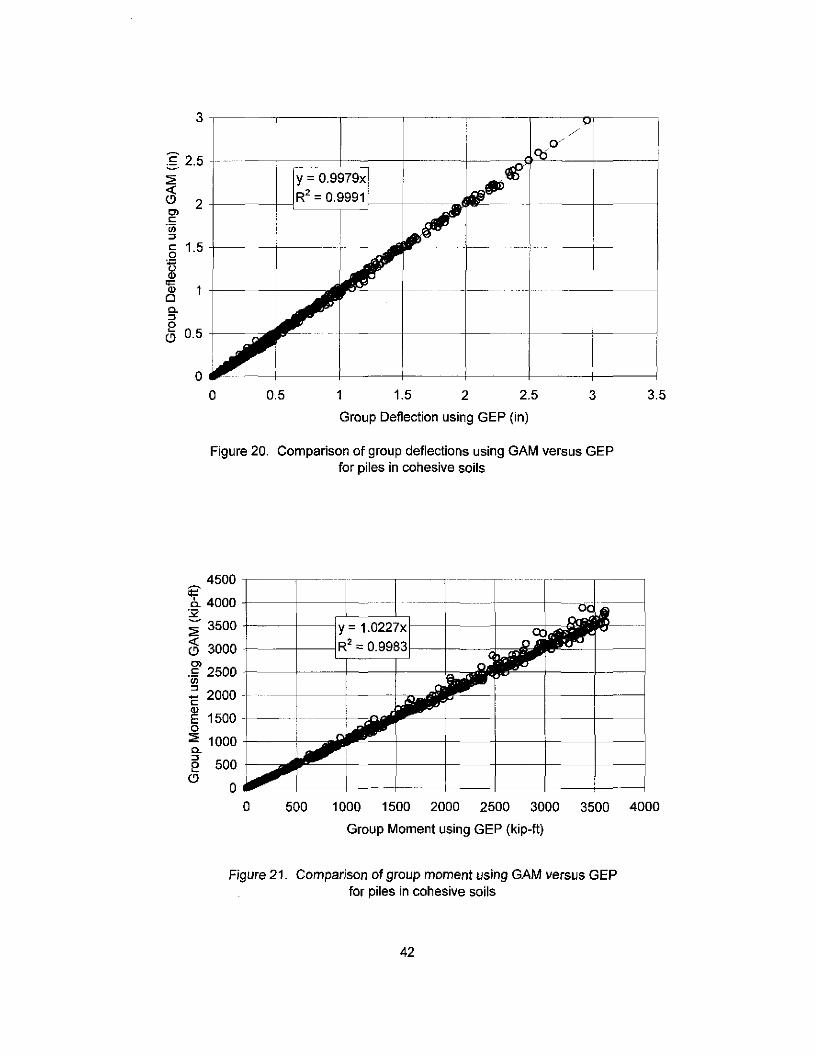
In Figures 20 through 23, the predicted values of deflection and moment

using the group amplification factor approach are compared with those from the

GEP procedure for pile groups in cohesive and cohesionless soils. It can be

seen that the new approach provides estimates of the group response

reasonably well with biases of no more than 2% and coefficients of determination

all above 0.99.

41

3,----,------,---,--------,------0,------,

3.532.521.510.5o

o

:? 2.5;2;

(3 2Cl t---(--{"-------"';='f-i-<::'iii:><:: 1.5 +------1---·-··i---~o

~'"~ 1+------1--a.:>e(!) 0.5 +--~

Group Deflection using GEP (in)

Figure 20. Comparison of group deflections using GAM versus GEPfor piles in cohesive soils

.. -_. -------I---+--

---,--',--

1000 1500 2000 2500 3000 3500 4000

Group Moment using GEP (kip-tt)

500

4500 ,-----,-

=b.. 4000 +---+---1--

~ 3500 ~--+---hY-:;=~1~.0n:2>?2~7XJ--+----+--=k(3 3000 1-1---fR~2~='.':0~.9~9~83T-I-<t;;jCl.5 2500 +----+---+---j----+-,...., .::.--+---+------1lJ):><:: 2000

~ 1500o;2; 1000 t----+-a.e 500 +----,:2iIIlIIIIII"""'--j------I----j---+---+---+------j

(!) 0-"'-----+---+---1----+--+----+---+---

o

Figure 21. Comparison of group moment using GAM versus GEPfor piles in cohesive soils

42

1.2 ,-------,-----,------------,------,-----,-----,

~--\------- - - -------

§ 1 +-------I----r--:;: y =0.9911x

(!j R2 = 0.9938C> 0.8 +----t-~~~~--_+-----:c----:c-;;

<::·iii:::l

<:: 0.6 +----+----+--o

~8 04 +------+--~a.:::l

§ 02 +-----:::0

o

0_2o ,....'-----+

o 0.4 0.6 0.8 1 1.2

Group Deflection using GEP (in)

Figure 22_ Comparison of group deflections using GAM versus GEPfor piles in cohesionless soils

y =0_9978x

R2 =0_9982

3500

4000

:;:(!j 3000 +----+-C>

.~ 2500 +---+--:::l~

-""m.9- 2000 +----+---Ee.~ 1500 +----+--+----;a.:::le 1000 +---+---....=---1--+--+---+---+(9

500 .l-----;-..'"--+----j---+---+--t---+-----j

oo 500 1000 1500 2000 2500 3000 3500 4000

Group Moment using GEP (kip-tt)

Figure 23. Comparison of group moment using GAM versus GEPfor piles in cohesionless soils

43

3.2.2 Steps for Simplified Analysis of Laterally Loaded Pile Groups

Steps for analyzing the behavior of laterally loaded pile groups using the

group amplification factor approach are as follows:

1) Using the pile and soil properties for the group to be analyzed, estimate the

lateral deflection and maximum moment of the single pile following the steps

presented in Section 3.1.3. The lateral load that should be used for the single

pile analysis is the lateral load on the pile group divided by the number of

piles (Npi1e) in the group.

2) Estimate the p-multipliers for each row of piles based on the center-to-center

spacing and pile row.

3) Add the p-multipliers for all the piles together (LPm).

4) Calculate Ay and Am using Equations 3.7 and 3.8, respectively.

5) Calculate the group deflection (yg) and maximum pile moment (Mg) using

Equations 3.5 and 3.6, respectively.

The limitations for the GAM include:

1. The group amplification factors were developed for pile groups no larger

than 5 x 5.

44

2. All the piles in each group must be identical.

3. The piles must be uniformly spaced.

4. This approach does not provide the load distribution among the piles in the

group nor the maximum moment of each pile with the exception of those in

the leading row.

5. Torsional effects are not considered in this study.

45

CHAPTER 4

COMPARISON OF PREDICTED WITH MEASURED VALUES FROM LOAD

TESTS

Several full-scale lateral load tests on fixed head pile groups have been

reported in the literature (Brown et aI., 2001; Huang et aI., 2001; Kim and

Brungraber, 1976; Mokwa and Duncan, 2000; Ng et aI., 2001; Rollins and

Sparks, 2002). The results for three case studies are compared with values

predicted using the procedures developed in this study, namely the MCLM and

the GAM. In general, the lateral loads applied in these load tests are either cyclic

incremental or they are performed following a Statnamic load test. This may lead

to a densification of cohesionless soils and a softening of cohesive soils.

Nevertheless for the cyclic load tests, the deflections and moments from the first

cycle of each load increment should closely approximate those from a static

loading condition, and are therefore useful for validating the analytical tools

developed herein.

4.1 Case Study 1 - Pile Group in Cohesive Soils

Rollins and Sparks (2002) performed two series of lateral load tests on a

fixed-head pile group at the Salt Lake City International Airport in Utah. A

Statnamic load test was performed to study the lateral response of the pile group

46

followed by a conventional static lateral load test. Loads for the static load test

were applied in the same direction as the Statnamic loads.

Nine piles, spaced three diameters apart center-to-center, were driven in a

3 x 3 arrangement. The piles were embedded in a 4-foot-thick and 9-foot-square

reinforced concrete pile cap. The pile cap was supported on six inches of

compacted granular fiJI. One side of the pile cap was compacted with granUlar fiJI

extending to the top of the pile cap (Figure 24) to provide passive resistance.

The piles consisted of 30-foot-long, 12%-inch-OD, 0.375-inch-thick-wall, concrete

filled, closed-end steel pipe piles.

The flexural rigidity (El) of the pile was estimated as follows:

(4.1)

where Is and Ie are the moment of inertia of the steel pipe and concrete,

respectively, Ee(= 2960 ksi based on fe' = 2700 psi) and Es (= 29,000 ksi) are the

Young's modulus of the concrete and steel, respectively. The flexural rigidity of

the pile composite was estimated to be 1.11x1 07 kip-in2.

47

(0)

,

Ib)

o 4

Ill-B

SHFFrrPIL£BEACTlONWAU.

W36X16ll

~-

Figure 24. Pile test layout for case study 1 (a) plan view, (b) and cross-section (Rollinsand Sparks, 2002)

Measured -.-. Predicted I

.-

.,,:"~- II'

_!_- --~ ---

---~p- ,

. 1---[::1Y-"

/Y ...

V"

700

Iii' 600Q.

;g, 500-cg: 400--'go 300e" 200.J!1a: 100

o0.0 0.5 1.0 1.5 2.0 2.5 3.0

Group Deflection (inches)

Figure 25. Comparison of measured versus predicteddeflections using GAM for case study 1

48

Subsurface soils at the site consist predominantly of soft clay. The natural

ground water table was reported to be immediately below the granular fill.

Rollins and Sparks neglected the soil resistance of the top four pile diameters to

account for a gap generated between the pile and the soil as a result of the

Statnamic testing. Based on this, the clay over the top 12 pile diameters had an

average undrained shear strength of 0.53 ksf. The undrained shear strength was

estimated based on triaxial unconsolidated undrained tests, vane shear tests,

and pressuremeter tests.

For this load test, the lateral resistance of the fixed head pile group can be

taken as the sum of the pile group and cap resistance. Rollins and Sparks

(2002) calculated the cap resistance and added it to the pile resistance at the

same deflection to obtain an overall load-deflection curve. They estimated the

pile group resistance at each value of deflection using GROUP. The pile group

resistance was also estimated using the methods developed in this study. The

predicted load-deflection curve compares quite favorably to the actual test results

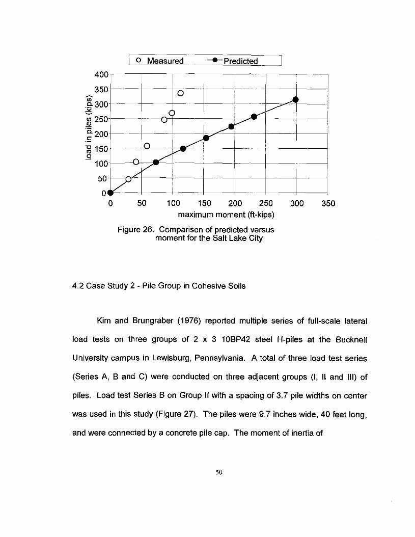
as shown in Figure 25. The calculated maximum bending moment did not

compare as favorably with the measured values for the piles in the leading row

as shown in Figure 26. This is probably due to rotation of the pile cap, which led

to a reduction in the maximum moment at the pile head. The estimated values of

moment are about 79 to 188 percent higher than the measured values.

49

I 0 Measured· --+- Predicted

I ··-li

.....

0 I

.....4 I- . - .

~1~~

,,........

~ I'--

I

'"'i ~.-,I

,.... ~ I

V -fI'" i

7 ,

i---_.~

50

400

350~

Ul.9- 300-'"~

Ul 250.~0.200<:

-g 150..Q

100

50

oo 100 150 200 250

maximum moment (ft-kips)

Figure 26. Comparison of predicted versusmoment for the Salt Lake City

300 350

4.2 Case Study 2 - Pile Group in Cohesive Soils

Kim and Brungraber (1976) reported multiple series of full-scale lateral

load tests on three groups of 2 x 3 10BP42 steel H-piles at the Bucknell

University campus in Lewisburg, Pennsylvania. A total of three load test series

(Series A, B and C) were conducted on three adjacent groups (I, II and III) of

piles. Load test Series B on Group II with a spacing of 3.7 pile widths on center

was used in this study (Figure 27). The piles were 9.7 inches wide, 40 feet long,

and were connected by a concrete pile cap. The moment of inertia of

50

4100-TON JACKSPILE WITH SLOPE 1 2 3INDICATOR TUBE IeJ IeJ IeJ 2 aD-TON JACKS l

\. 3.0 I

P-l5 6

14 !'"2.0L

~ 2.0 r-3.0 3.0 2.0 I-

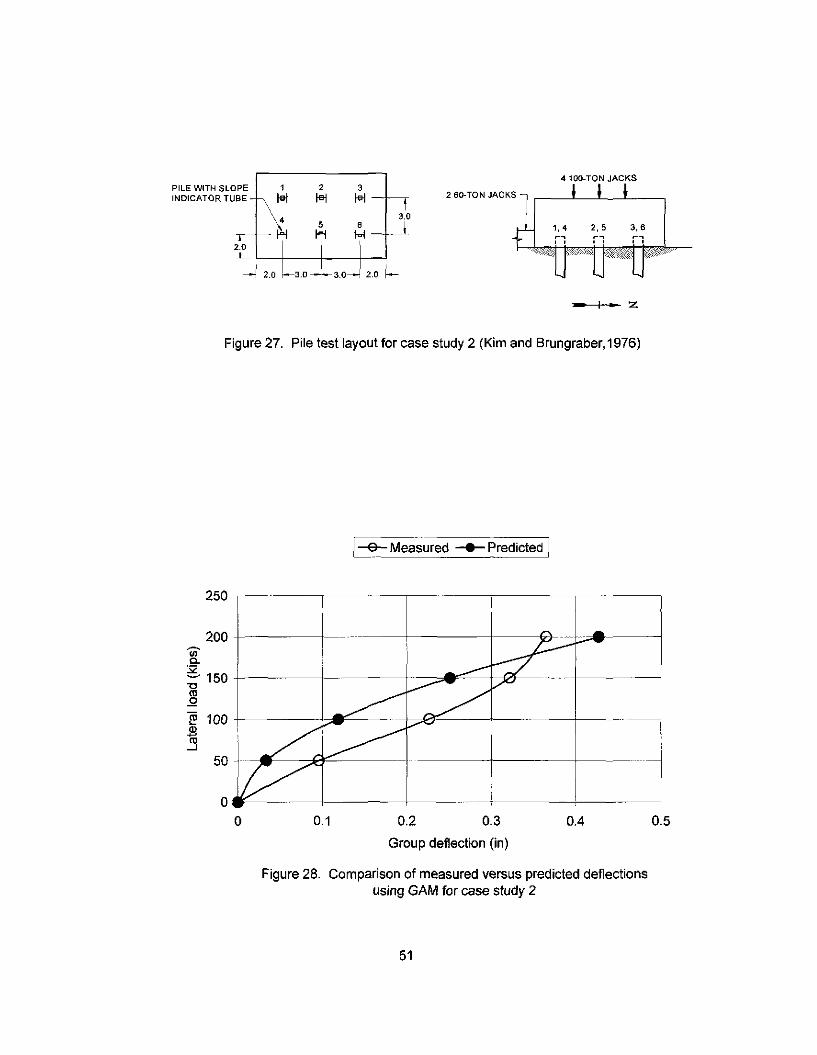
Figure 27. Pile test layout for case study 2 (Kim and Brungraber, 1976)

Eo Mea·~ured -... Predicted I

250 ,-----,---

200+----+_

~ JI

0.1 0.2 0.3 0.4 0.5

0.-

o

R:52~ 150 +----+_1::>m.Q

~ 100 +-----+__,.-::--- -he-=------+-----+--.l!lj

Group deflection (in)

Figure 28. Comparison of measured versus predicted defiectionsusing GAM for case study 2

51

the pile was 224.2 in4. The pile cap was 4 feet thick, 10 feet long and 8 feet

wide.

Subsurface conditions over the top 8 shaft diameters consisted of silty

clay with an average undrained shear strength of 2.5 ksf, estimated based on

unconfined compression tests and standard penetration test data. The ground

water table was reported to be at a depth of 35 feet.

In this load test, the cap was at the ground surface with zero embedment.

As a result, the pile cap resistance is not considered significant and the lateral

resistance can be considered to be due primarily to the pile group. An axial load

of 72 kips per pile was applied. The lateral load-deflection curve for the group

was estimated using the procedures developed and is compared to measured

values in Figure 28. The measured load deflection curve compares reasonably

with the calculated curve. Note that the measured deflections increased by only

70 percent and measured moments increased by only 42 percent when the load

was doubled. This indicates inconsistency in the measurements, because these

quantities would increase by a factor of two or higher if the behavior was truly

nonlinear.

The lateral load-moment curve for the group was estimated using the

procedures developed and compared to average measured values of the piles in

the leading row. Figure 29 showed that the estimated maximum bending52

moments are nine percents below to 52 percent higher than the measured value

for the leading row of piles.

[ 0 Measured Moment·...:..- Predicted Moment I

~..

!~i 0i

-----V- i

./ ic---0 j

---

......V

--

/'"i l.e'

/'

./ !-

35

30

"[ 25g.91 20.5.

(;; 150

."11 10

5

oo 20 40 60 80 100 120 140 160

maximum moment (kip~fl)

Figure 29. Comparison of predicted versus measured bendingmoment for Bucknell University load test

4.3 Case Study 3 - Pile Group in Cohesionless Soils

Huang et al. (2001) and Brown et al. (2001) reported a full-scale lateral

load test on a group of six bored piles reacting against a group of twelve precast

concrete piles for the proposed high-speed rail system project in Taipao

Township of Chaiyi County, Taiwan. The bored piles had a diameter of 59

inches, were 114 feet long, spaced 3 diameters on center and were connected53

by a pile cap. The flexural stiffness of the drilled shaft was 2.39 x 109 kip-in2.

The pile cap was 6.5 feet thick, 72 feet long and 49 feet wide. Subsurface

conditions over the top 8 shaft diameters consisted of loose silty sand with an

average friction angle of 35 degrees (Brown et aI., 2001). The ground water

table was reported to be at a depth of 3.3 feet. The p-multipliers for the first,

second and third rows are 0.5, 0.4 and 0.3, respectively (Brown et aI., 2001).

In this load test, the cap was at the ground surface with zero embedment

(Figure 30). As a result, the pile cap resistance is not considered to be

significant and the lateral resistance can be considered to be due primarily to the

pile group. The lateral load-deflection curve for the group is estimated using the

procedures developed and is compared to measured values in Figure 31. It can

be seen that in general, there is good agreement between the estimated

deflections and the measured values. The estimated maximum bending moment

(8,850 kip-ft) was 23 percent lower than the measured value in the leading row

(11,551 kip-ttl. Only one value of bending moment was published corresponding

to a lateral load of 41 0 kips.

54

PC Piles

Figure 30. pile test layout for case study 3 (Huang et al., 2001)

E() M~~sured ....... predicted]

_.

I! !

,

~~

~....... I

~-;;;w

I

#'~

iI

3000

2500

"'a.g 2000

~ 1500

e!"* 1000-'

500

o0.00 0.20 0.40 0.60 0.80 1.00 1.20 1.40

Group deflection (in)

Figure 31. Comparison of measured versus predicted deflectionsusing GAM for case study 3

55

CHAPTER 5

SUMMARY AND CONCLUSIONS

The Modified Characteristic Load Method (MCLM) was developed for

estimating single pile head deflection and maximum bending moment for fixed

head piles embedded below ground surface in cohesive soils. This simple

procedure requires pile diameter, pile elastic modulus, moment of inertia, pile

head embedment depth, undrained shear strength and soil unit weight as input

parameters. The MCLM provides reliable values of pile deflections and

maximum moments when compared with LPILE Plus.

The Group Amplification Method (GAM) was developed to predict the

lateral behavior of fixed-head pile groups. This procedure was derived based on

the group equivalent pile method proposed by Mokwa and Duncan (2000). The

GAM can be used to amplify the single pile deflection and bending moment to

predict the pile group deflection and maximum moment. The amplification

factors depend on the number of piles in the group, pile spacing and p

multipliers. The p-multipliers depend on soil type, pile spacing, pile position

within the group relative to the direction of the applied force and construction

method.

56

The GAM in conjunction with the MCLM was used to predict the behavior

of three full-scale pile groups that were load tested. These predictions indicate

that the procedures provide estimates of group deflections and moments that are

accurate enough for most practical purposes or they provide results that err on

the side of conservatism.

57

REFERENCES

Bretlmann, T., and Duncan, J.M. (1996). "Computer Application of CLM Lateral

Load Analysis to Piles and Drilled Shafts." ASCE, Journal of Geotechnical

Engineering, 122(6) 496-498.

Bridge Software Institute, University of Florida, accessed 2003, http://bsi

web.ce.ufl.edu

Brown, DA, Reese, LC., and O'Neill, MW. (1987). "Cyclic Lateral Loading of a

Large Scale Pile Group." ASCE, Journal of Geotechnical Engineering,

113(11),1326-1343.

Brown, DA, Morrison, C., and Reese, LC. (1988). "Lateral Load Behavior of

Pile Group in Sand." ASCE, Journal of Geotechnical Engineering,

114(11),1261-1276.

Brown, DA, and Bollman, HT (1993). "Pile-supported Bridge Foundations

Designed for Impact Loading." Appended document to the Proceedings of

Design of Highway Bridges for Extreme Events, Crystal City, Virginia, 265

281.

Brown, DA, O'Neill, MW., Hoit, M., McVay, M., EI Naggar, M. H., Chakrabory,

S. (2001). "Static and Dynamic Lateral Loading of Pile Groups." NCHRP

Report 461, Transportation Research Board, National Research Council.

58

Duncan, J.M., Evans, L.T. Jr. and Ooi, P.S.K. (1994). "Lateral Load Analysis of

Single Piles and Drilled Shafts." ASCE, Journal of Geotechnical

Engineering, 120(6), 1018-1033.

Evans, L.T. Jr. and Duncan, J.M. (1982). "Simplified Analysis of Laterally

Loaded Piles." Rep. No. UCB/GT/82-04, University of California,

Berkeley, Calif.

Franke, E. (1988). "Group Action Between Vertical Piles under Horizontal

Loads." WF. Van Impe, ed. A.A. Balkema, Rotterdam, The Netherlands,

83-93.

Hannigan, P.J., Goble, G.G., Thendean, G., Likins, G.E. and Rausche, F.

(1997). "Design and Construction of Driven Pile Foundations." FHWA

Publication No. FHWA-HI-97-013, NTIS, Springfield, Virginia.

Huang, A., Hsueh, C., O'Neill, MW., Chern, S. and Chen, C. (2001). "Effects of

Construction on Laterally Loaded Pile Groups." ASCE, Journal of

Geotechnical and Geoenvironmental Engineering, 127(5), 385-397.

Kim, J.B., and Brungraber, R.J. (1976). "Full-Scale Lateral Load Tests of Pile

Groups." ASCE, Journal of Geotechnical Engineering, 102(1), 87-105.

Matlock, H. (1970). "Correlations for Deign of Laterally-Loaded Piles in Soft

Clay." Paper No. OTC 1204, Proceedings, Second Annual Offshore

Technology Conference, Houston, Texas, Vol. 1, 577-594.

59

McVay, M., Casper, R and Shang, T.!. (1995). "Lateral Response of Three Row

Groups in Loose to Dense Sands at 3D and 50 Spacings." ASCE,

Journal of Geotechnical Engineering, 121 (5), 436-441.

McVay, M., Zhang, L., Molnit, T and Lai, P. (1998). "Centrifuge Testing of Large

Laterally Loaded Pile Groups in Sands." ASCE, Journal of Geotechnical

and Geoenvironmental Engineering, 124(10), 1016-1026.

Meimon, Y., Baguelin, F., and Jezequel, J.F. (1986). "Pile Group Behavior

under Long Time Lateral Monotonic and Cyclic Loading." Proc., 3rd Int.

Conf on Numerical Methods in Offshore Piling, Nantes, France, Editions

Technip, 285-302.

Mokwa, RL., and Duncan, J.M. (2000). "Investigation of the Resistance of Pile

Caps and Integral Abutments to Lateral Loading." Research report

submitted to the Virginia Transportation Research Council, Report No.

VTRC OO-CR4, Charlottesville, Virginia.

Mokwa, RL., and Duncan, J.M. (2001). "Laterally Loaded Pile Group Effects

and p-y Multipliers." ASCE Special Publication No. 113, Foundation and

Ground Improvement, 729-742.

Ng, C., Zhang, L., and Nip, D. (2001). "Response of Laterally Loaded Large

Diameter Bored Pile Groups." ASCE, Journal of Geotechnical and

Geoenvironmental Engineering, 127, (8) 658-669.

60

Pinto, P., McVay, M., Hoit, M. and Lai, P. (1997). "Centrifuge Testing of Plumb

and Battered Pile Groups in Sand." TRB Rec. No. 1569. Transp. Res.

Board, Washington D.C., 8-16.

Reese, L.C., and Welch, R.C. (1975). "Lateral Loading of Deep Foundations in

Stiff Clay." ASCE, Journal of Geotechnical Engineering, 101 (7),633-649.

Reese, L.C. and Wang, S-T. (1996). Group 4.0 for Windows, Analysis of a

Group of Piles Subjected to Axial and Lateral Loading. Ensoft, Inc.,

Austin, Tex.

Reese, L.C., and Wang, S-T. (1997). LPILE PLUS 3.0 for Windows. Ensoft,

Inc., Austin, Tex.

Rollins, K.M., Peterson, K.T., and Weaver, T.J. (1998). "Lateral Load Behavior of

a Full-Scale Pile Group in Clay." ASCE, Journal of Geotechnical and

Geoenvironmental Engineering, 124(6),468-478.

Rollins, K.M., and Sparks, A.E. (2002). "Lateral Resistance of Full-Scale Pile

Cap with Gravel Backfill." ASCE, Journal of Geotechnical and

Geoenvironmental Engineering, 128(9) 711-723.

Ruesta, P.F., and Townsend, F.C. (1997). "Evaluation of Laterally Loaded Pile

Group at Roosevelt Bridge." ASCE, Journal of Geotechnical and

Geoenvironmental Engineering, 123(12), 1153-1161.

Sparks, A. and Rollins, K.M. (1997). "Passive Resistance and Lateral Load

Capacity of a Full-scale Fixed-head Pile Group in Clay." Civ. Engrg. Dept.

Res. Rep. CEG.97-04, Brigham Young Univ., Provo, Utah.

61

Wang, S. (2000). "Simplified Analysis for Laterally Loaded Piles in Cohesionless

Soils." Repott submitted to the University of Hawaii in pattial fulfillment for

the degree of Master of Science in Civil Engineering. University of

Hawai'i, Honolulu, HI.

Zhang, X. (1999). "Comparison of Lateral Group Effects Between Bored and PC

Driven Pile Groups in Sand." M.S. thesis. University of Houston, Tex.

62

university of hawai1ljbrary simplified procedure for - scholarspace

Documents