UniversityofHohenheim

InstituteofSoilScienceandLandEvaluation

Mapping of soil organic carbon and nitrogen in two small adjacent Arctic watersheds on Herschel Island, Yukon

Territory

Master-Thesis (30 ECTS) Agricultural Sciences- Major Soil Sciences

Isabell Eischeid (588881) 02.11.2015

First examiner: Prof. Dr. Thilo Streck Second examiner: Prof. Dr. Hugues Lantuit

ii

Table of Contents ListofFigures....................................................................................................................................................................iv 

ListofTables.......................................................................................................................................................................v 

ListofAbbreviations......................................................................................................................................................vi 

Abstract................................................................................................................................................................................1 

1.Introduction...................................................................................................................................................................2 

2.Background....................................................................................................................................................................5 

2.1Cryosols....................................................................................................................................................................5 

Definition...................................................................................................................................................................5 

Threepartmodel....................................................................................................................................................6 

DistributionofCryosols.......................................................................................................................................8 

2.2Watersheddisturbances...................................................................................................................................9 

Coldenvironmentdisturbances.......................................................................................................................9 

Temperatureindependentslopeprocesses..............................................................................................11 

2.3EcologicalandvegetationclassesofHerschelIsland..........................................................................12 

VegetationClasses................................................................................................................................................12 

EcologicalClasses.................................................................................................................................................14 

3.Methods.........................................................................................................................................................................18 

3.1StudySite...............................................................................................................................................................18 

HerschelIsland......................................................................................................................................................18 

IceCreekwatershed............................................................................................................................................19 

3.2Selectionofsamplinglocations....................................................................................................................20 

RemoteSensing.....................................................................................................................................................20 

GroundTruthing...................................................................................................................................................20 

3.3Fieldwork.............................................................................................................................................................22 

3.4Imageprocessing...............................................................................................................................................23 

Aerialimage............................................................................................................................................................23 

Atmosphericprocessing....................................................................................................................................23 

Georeferencing......................................................................................................................................................23 

3.5RemoteSensing...................................................................................................................................................24 

TrainingUnits........................................................................................................................................................24 

SpectralClassification.........................................................................................................................................24 

PostProcessing......................................................................................................................................................24 

GroundTruthing...................................................................................................................................................24 

3.6LaboratoryMethods.........................................................................................................................................25 

Drybulkdensityandwatercontent.............................................................................................................25 

Grainsizedistribution........................................................................................................................................25 

TotalCarbon,NitrogenandTotalOrganicCarbon.................................................................................26 

iii

3.7Dataprocessingandanalysis........................................................................................................................27 

Locationproperties.............................................................................................................................................27 

Soilcharacteristics...............................................................................................................................................28 

Vegetationdata......................................................................................................................................................28 

Boxplotsforecologicalandvegetationclassesandwatershed.........................................................28 

NMDS.........................................................................................................................................................................28 

PCA..............................................................................................................................................................................29 

Landcovercomparisons.....................................................................................................................................29 

Furtherstatisticalanalysis................................................................................................................................29 

4.Results............................................................................................................................................................................30 

4.1Remotesensing...................................................................................................................................................30 

ClassificationSystem...........................................................................................................................................30 

Ecologicalandvegetationclasses..................................................................................................................30 

GroundTruthing...................................................................................................................................................33 

4.2Ordination.............................................................................................................................................................35 

NMDS.........................................................................................................................................................................35 

PCA..............................................................................................................................................................................36 

4.3IceCreektotalorganiccarbonandnitrogenstorage..........................................................................38 

Terrain......................................................................................................................................................................38 

EcologicalClasses.................................................................................................................................................38 

Transects..................................................................................................................................................................46 

5.Discussion.....................................................................................................................................................................49 

5.1Remotesensingclassification.......................................................................................................................50 

Detectability............................................................................................................................................................50 

Effectivenessofclassification..........................................................................................................................53 

5.2Spatialdistributionoftotalorganiccarbonandnitrogen.................................................................57 

Terrain......................................................................................................................................................................59 

EcologicalClassApproach................................................................................................................................64 

Transectbasedapproach..................................................................................................................................67 

5.3IceCreekwatershedandclimatechange.................................................................................................70 

6.Conclusion....................................................................................................................................................................73 

7.References....................................................................................................................................................................vii 

Acknowledgements......................................................................................................................................................xiii 

Appendix...........................................................................................................................................................................xiv 

EidesstattlicheErklärung........................................................................................................................................xxiii 

iv

List of Figures

Figure1:Circum‐arcticpermafrostdistribution(Brownetal.,1998).............................................................8 

Figure2:Herschelecologicalclass.................................................................................................................................14 

Figure3:Komakukecologicalclass...............................................................................................................................15 

Figure4:Plover‐Jaegerecologicalclass.......................................................................................................................15 

Figure5:Thrasherecologicalclass................................................................................................................................16 

Figure6:ShrubZoneecologicalclass...........................................................................................................................16 

Figure7:WetTerrainecologicalclass..........................................................................................................................17 

Figure8:LocationofHerschelIsland...........................................................................................................................18 

Figure9:IceCreekEastandWest..................................................................................................................................19 

Figure10:Overviewofthestudyarea.........................................................................................................................21 

Figure11:ClassificationoftheIceCreekwatershed.............................................................................................31 

Figure12:Highlightsofstudyareawherethevegetationtypedoesnotcoincidewiththe

typicallyassociatedecologicalclass..............................................................................................................................32 

Figure13:Non‐metricmultidimensionalscaling(NMDS)offorbsandshrubsat66sampling

locations....................................................................................................................................................................................35 

Figure14:Principalcomponentanalysisofsoilpropertiesat23samplinglocationswith

ecologicalclasses...................................................................................................................................................................37 

Figure15:Principalcomponentanalysisofsoilpropertiesat23samplinglocationswith

vegetationclasses..................................................................................................................................................................37 

Figure16:Totalorganiccarbon(kg/m²)at0‐30cmandtheentireextentoftheactivelayerin

IceCreekwatershedonHerschelIsland.....................................................................................................................39 

Figure17:Totalnitrogen(kg/m²)at0‐30cmandtheentireextentoftheactivelayerinIce

CreekwatershedonHerschelIsland.............................................................................................................................40 

Figure18:ComparisonofTOC(kg/m²)inthefirst30cmandtheentireactivelayerofthesoil

betweenecologicalandvegetationclasses................................................................................................................43 

Figure19:ComparisonofTN(kg/m²)inthefirst30cmandtheentireactivelayerofthesoil

betweenecologicalandvegetationclasses................................................................................................................44 

Figure20:ComparisonofCNratiosinthefirst30cmandtheentireactivelayerofthesoilas

wellasactivelayerdepthbetweenecologicalandvegetationclasses............................................................45 

Figure21:Totalorganiccarbon(kg/m²)ateachsamplingpointonthreetransectsacrosstheIce

Creekwatershed....................................................................................................................................................................47 

Figure22:BoxplotscomparingthedifferencesinTOC,TNandCNratiosbetweenanupper,

middleandlowertransectwithintheIceCreekWatershed...............................................................................48 

v

List of Tables

Table1:Cryosolicorders......................................................................................................................................................6 

Table2:Associationofvegetationtypestoecologicalclasses...........................................................................30 

Table3:Classificationaccuracybetweenobserved(groundtruthing)andpredicted

(classification)ecologicalunits.......................................................................................................................................33 

Table4:Classificationaccuracybetweenobserved(groundtruthing)andpredicted

(classification)vegetationunits......................................................................................................................................34 

Table5:Spearman’srankcorrelation(ρ)ofTWI(topographicwetnessindex),moisturein

topsoil,NDVI(normalizeddifferencevegetationindex)andslope(indegrees)withTOC(total

organiccarbon),TN(totalnitrogen)andtheCNratio..........................................................................................38 

Table6:Averagesofsoilandlandscapepropertiesforeachecologicalclass.............................................41 

Table7:ComparisonofareacoveredbyecologicalclassesandTOC,TNstorageinIceCreek

WestandEast..........................................................................................................................................................................42 

vi

List of Abbreviations

ALD Activelayerdetachment

ANOVA Analysisofvariance

CN Organiccarbontonitrogenratio

DEM Digitalelevationmodel

HE Herschel

HK Herschel‐Komakuk

IC IceCreek

ICE IceCreekEast

ICW IceCreekWest

KO Komakuk

NDVI Normalizeddifferencevegetationindex

NMDS Non‐metricmultidimensionalscaling

PCA Principalcomponentanalysis

PJ Plover‐Jaeger

RTS Retrogressivethawslump

SOC Soilorganiccarbon

SZ ShrubZone

TH Thrasher

TN Totalnitrogen

TOC Totalorganiccarbon

TWI Topographicwetnessindex

WT WetTerrain

1

Abstract

Permafrost soils are particularly vulnerable to global climate change, and warming airtemperatures could turn them from carbon sinks into carbon sources. Estimates of Arcticcarbon stocks are still highlyuncertain, despite their importance topredict themagnitudeofCO2 and CH4 release to the atmosphere, a process termed the Permafrost Carbon Feedback.BecausemostoftheArcticisdifficulttoaccessandsurvey,remotesensingtechniquesbearthecapacitytofillspatialgapsandmapthechanginglandscapeatwiderscales.Recentstudieshaveattempted to usemultispectral images, such as Landsat, to estimate soil total organic carbon(TOC)and totalnitrogen (TN)storage.Yet,most studiesworkedona regional toglobal scaleandusedrelativelycoarse landscapeclasses.SinceTOCandTNstorage isknowntobehighlyspatially variable in the landscape, high resolution estimates of TOC and TN storage arenecessarytoestimatethepotentialimpactofthawingpermafrost(andthesubsequentreleaseofCO2andCH4)totheatmosphere.Thisprojectisoneofthefirsttousehighresolutionimages(1.65m GeoEye (4 spectral bands: blue‐infrared), 2m DEM) to predict SOC and TN storagewithin different Tundra vegetation classes in a small (3 km²) twinwatershed (Ice Creek) onHerschel Island, Yukon, Canada. Vegetation classes were based on indicator species andgeomorphic disturbance levels. Remote sensing detection accuracy varied strongly betweenclasses.Fieldbasedmoisturemeasurementsweremoststronglycorrelatedwiththecarbontonitrogen (CN) ratio, TOC and TN (ρ =0.84, ρ =0.74 ρ =0.65, p<0.05). However, slope and thenormalizeddifferencevegetationindex(NDVI)alsohadastatisticallysignificantrelationshiptoCNandTOC.Thissuggeststhatfinescaleestimatesofcarbonandnitrogenstocksarepossibleusingfewspectralbandsfromhighresolutionimages.TheactivelayerofIceCreekwatershedcontains33391 tonnesofTOCand3635 tonnesofTN,which is lower than theaveragevaluereported forHerschel Island by theNorthern Circumpolar Soil CarbonDatabase. Carbon andnitrogenarenotevenlydistributedwithinthewatershed.Flatuplandterrainandtallerectbushareascontainedthe largestamountTOCandTN.Lowestcontentscouldbe found in thesteepand frequentlyerodedzones.Highcarbonaccumulationalongthestreambankssuggests thatfluvialprocessesdonotremovealltheerodedsedimentsfromthewatershed.Anintensificationof summer rainfall and warmer temperatures could alter the hydrological patterns of thewatershedandcurrentaccumulationsitesmayreleasemorecarbonfromthecatchmentstotheBeaufort Sea.High correlationbetween soilmoisture andTOCandTN contents found in thisthesis shows that moisture information retrieved from satellite radar data could provideadditional information on soil properties. This thesis also shows that detailed studies onremobilization of carbon in the catchments and atmospheric losses of carbon are crucial tounderstandtherolesmallwatershedsplayinthefaceofachangingclimate.

2

1. Introduction

Thedetectedandprojectedclimate change isparticularly severe in theArctic regionbecause

changesincloudcoverandseaicesignificantlyalterthethermalbalanceofthisarea(Holland&

Bitz,2003).Temperaturesareexpectedtoincreaseandprecipitationpatternsmaychangemore

rapidly than in other parts of the world (IPCC, 2007). Precipitation patterns in cold

environmentsareparticularly important for landscapedynamicsandnutrient turnover in the

soil. Higher snowfall insulates the soil in the winter and promotes higher rates or

mineralization,whereasatthesametimelatesnowmeltshortensthegrowingseasonbyuptoa

monthandaltersvegetationdistribution(Jonesetal.,2011;Cooper,2014).Intensiverainfallin

latesummer,wheretheactivelayerofthepermafrostisdeepestcanresultinmasswastingand

erosionevents(Lamoureuxetal.,2014).

In most cold environments, organic matter accumulation is high because low temperatures

preventhighnutrient turnover rates (Hobbieetal.,2000).Furthermore, cryoturbationburies

organicmatterrich topsoilsand locks themfrommineralization(Bockheim,2015).Therefore

arcticsoilshavehighorganiccarboncontentsthathavebeenpartoflongtermstorage(Hobbie

etal.,2000,Hugeliusetal.,2014).Highcarbonstoragemeansthatthawingofpermafrostcould

potentiallyhavelargeimpactontheEarth’sclimate,turningthemfromcarbonsinksintocarbon

sources (Schuur,2015).Permafrost thaw ispartof a self‐acceleratingprocesswhere thawing

releases more greenhouse gases which in turn enhance the climate change and is therefore

difficulttoslowdown(Schuur,2015).ThisprocessistermedthePermafrostCarbonFeedback

(Schaefer et al, 2014). Several major research projects aim to estimate global arctic carbon

stocks but estimates are still highly uncertain, despite their importance to predict the

magnitudeofCO2andCH4release to theatmosphere (Hugeliusetal.,2014).Additionally, the

roleandquantityofnitrogeninthesesoilshasbeenlargelyunstudied.Nitrogenplaysamajor

role in carbonmineralization, but its presence can lead to the release of the greenhouse gas

nitrousoxide(NO2)Todate,onlyveryfewstudieshavetriedtoestimatenitrogenstocksinthe

arctic(Obuetal.,2015).

Loose sediments moved during the last glaciation are held together in the frozen state by

permafrost.Thawingpermafrostisthereforeparticularlysusceptibletoerosion(Lamoureux&

Lafrenière,2014).Everyyear,duringthefewmonthswheretemperaturesareabovezero,the

arcticlandscapebecomesverydynamic.Coastalareasareundergoingerosionandslumping,the

activelayerofthepermafrostmaydetachinmasswastingeventsandthermalerosionchannels

maymovelargeamountsofsedimentsandorganicmatterwithinthelandscapeorintothesea

(Pautler et al., 2010; Lantuit et al., 2012;Harms et al., 2014). The contribution frommost of

3

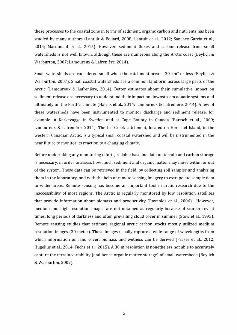
theseprocessestothecoastalzoneintermsofsediment,organiccarbonandnutrientshasbeen

studied bymany authors (Lantuit& Pollard, 2008; Lantuit et al., 2012; Sánchez‐García et al.,

2014; Macdonald et al., 2015). However, sediment fluxes and carbon release from small

watersheds isnotwellknown,althoughthesearenumerousalongtheArcticcoast(Beylich&

Warburton,2007;Lamoureux&Lafrenière,2014).

Smallwatershedsareconsideredsmallwhen thecatchmentarea is30km2or less (Beylich&

Warburton,2007).Smallcoastalwatershedsareacommonlandformacross largepartsofthe

Arctic (Lamoureux & Lafrenière, 2014). Better estimates about their cumulative impact on

sedimentreleasearenecessarytounderstandtheirimpactondownstreamaquaticsystemsand

ultimatelyontheEarth’sclimate(Harmsetal.,2014;Lamoureux&Lafrenière,2014).Afewof

these watersheds have been instrumented to monitor discharge and sediment release, for

example in Kärkevagge in Sweden and at Cape Bounty in Canada (Bartsch et al., 2009;

Lamoureux & Lafrenière, 2014). The Ice Creek catchment, located on Herschel Island, in the

westernCanadianArctic, isa typical small coastalwatershedandwillbe instrumented in the

nearfuturetomonitoritsreactiontoachangingclimate.

Beforeundertakinganymonitoringefforts,reliablebaselinedataonterrainandcarbonstorage

isnecessary,inordertoassesshowmuchsedimentandorganicmattermaymovewithinorout

ofthesystem.Thesedatacanberetrievedinthefield,bycollectingsoilsamplesandanalyzing

theminthelaboratory,andwiththehelpofremotesensingimagerytoextrapolatesampledata

to wider areas. Remote sensing has become an important tool in arctic research due to the

inaccessibility ofmost regions. The Arctic is regularlymonitored by low resolution satellites

that provide information about biomass and productivity (Raynolds et al., 2006). However,

medium and high resolution images are not obtained as regularly because of scarcer revisit

times,longperiodsofdarknessandoftenprevailingcloudcoverinsummer(Stowetal.,1993).

Remote sensing studies that estimate regional arctic carbon stocks mostly utilized medium

resolutionimages(30meter).Theseimagesusuallycaptureawiderangeofwavelengthsfrom

which information on land cover, biomass and wetness can be derived (Fraser et al., 2012,

Hugeliusetal.,2014,Fuchsetal.,2015).A30mresolutionisnonethelessnotabletoaccurately

capturetheterrainvariability(andhenceorganicmatterstorage)ofsmallwatersheds(Beylich

&Warburton,2007).

4

ThisstudywilltestthesuitabilityofcombiningtwometerresolutionGeoEyeimageswithfield

surveys to accurately predict soil organic carbon and nitrogen storage in the Ice Creek

watershed on Herschel Island, western Canadian Arctic. The high resolution outputs of this

thesis will be compared with other datasets, such as the Northern Circumpolar Soil Carbon

Database (Hugelius et al., 2013) to inform future upscaling strategies. It will also provide

baselinedataforfuturehydrologicalstudieswithintheIceCreekwatershedonHerschelIsland.

Thereweretwomajorobjectivesofthisstudy:

1) Totestthesuitabilityofusingecologicalclasses(whichincludeaqualitativeassessment

of vegetation, slope and disturbances) and simple vegetation classes to predict soil

organic carbon (TOC) and nitrogen (TN)within the Ice Creekwatershed onHerschel

Island.

Suitableisdefinedas:

a) DetectablethroughremotesensingmethodswithGeoEyeimages

b) CharacterisedbylowvariationwithinandlowredundancyofTOCandTNcontents

betweenclasses

2) To analyze and discuss the spatial distribution of soil organic carbon and nitrogen

withintheactivelayerofIceCreekwatershed.Andmorespecifically:

a. EvaluatehowterraincharacteristicsaffectTOCandTNstorage

b. UseecologicalclassestounderstandhowbioticandabioticfactorsinfluenceTOC

andTNaccumulation

c. Use cross sections through the watershed to identify TOC mobilization and

accumulationsites

5

2. Background

2.1 Cryosols

Definition ThewordCryosolcomesfromtheGreekwordsforicy‐coldandsoil.Theconceptthatfrozen

soils need their own study and classification systemwas introduced to the English speaking

world by the Russian researcher Nikiforoff in 1928 (in Bockheim, 2015). For a couple of

decades,therehasbeenhesitationaboutclassifyingfrozensoilsasrealsoilsbecausebiological

andchemical activity is limited in the frozenstate (Bockheim,2015).However, since2006, it

hasbeenacceptedasakeysoilgroupintheWorldReferenceBaseforSoils(WRB).Itisdefined

as“soilshavingoneormorecryichorizonswithin100cmfromthesoilsurface”.Whereascryic

is:“aperenniallyfrozensoilhorizoninmineralororganicmaterials”.

Acryichorizonhas:

1. continuouslyfor≥2consecutiveyearsoneofthefollowing:

a. massiveice,cementationbyiceorreadilyvisibleicecrystals;or

b. asoiltemperatureof≤0°Candinsufficientwatertoformreadilyvisibleicecrystals;

and

2. athicknessof≥5cm

(IUSSWorkingGroup,2014)TheCanadianSystemofSoilClassification(CSSC,1988)hasaseparateorderforCryosolsand

definesthemasfollows:“Cryosolicsoilsareformedineithermineralororganicmaterialsthat

havepermafrosteitherwithin1mofthesurfaceorwithin2mifthepedonhasbeenstrongly

cryoturbated laterally within the active layer, as indicated by disrupted, mixed, or broken

horizons. They have amean annual temperature ≤0°C. Differentiation of Cryosolic soils from

soilsof otherorders involves eitherdeterminingor estimating thedepth topermafrost.”The

Canadian system then further divides the Cryosolic order into three great groups: Turbic

Cryosols,StaticCryosolsandOrganicCryosols.Table1describesthedefiningcharacteristicsof

thesegreatgroups(CSSC,1988)

6

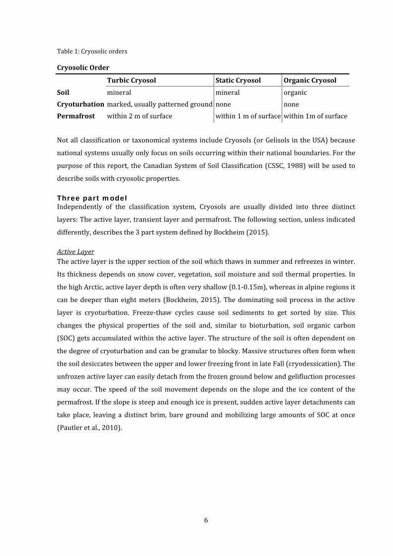
Table1:Cryosolicorders

CryosolicOrder

TurbicCryosol StaticCryosol OrganicCryosol

Soil mineral mineral organic

Cryoturbationmarked,usuallypatternedground none none

Permafrost within2mofsurface within1mofsurfacewithin1mofsurface

NotallclassificationortaxonomicalsystemsincludeCryosols(orGelisolsintheUSA)because

nationalsystemsusuallyonlyfocusonsoilsoccurringwithintheirnationalboundaries.Forthe

purposeof thisreport, theCanadianSystemofSoilClassification(CSSC,1988)willbeusedto

describesoilswithcryosolicproperties.

Three part model Independently of the classification system, Cryosols are usually divided into three distinct

layers:Theactivelayer,transientlayerandpermafrost.Thefollowingsection,unlessindicated

differently,describesthe3partsystemdefinedbyBockheim(2015).

ActiveLayerTheactivelayeristheuppersectionofthesoilwhichthawsinsummerandrefreezesinwinter.

Its thicknessdependsonsnowcover,vegetation,soilmoistureandsoil thermalproperties. In

thehighArctic,activelayerdepthisoftenveryshallow(0.1‐0.15m),whereasinalpineregionsit

canbedeeper thaneightmeters (Bockheim,2015).Thedominating soilprocess in theactive

layer is cryoturbation. Freeze‐thaw cycles cause soil sediments to get sorted by size. This

changes the physical properties of the soil and, similar to bioturbation, soil organic carbon

(SOC)getsaccumulatedwithintheactivelayer.Thestructureofthesoilisoftendependenton

thedegreeofcryoturbationandcanbegranulartoblocky.Massivestructuresoftenformwhen

thesoildesiccatesbetweentheupperandlowerfreezingfrontinlateFall(cryodessication).The

unfrozenactivelayercaneasilydetachfromthefrozengroundbelowandgelifluctionprocesses

may occur. The speed of the soilmovement depends on the slope and the ice content of the

permafrost.Iftheslopeissteepandenoughiceispresent,suddenactivelayerdetachmentscan

takeplace, leaving adistinct brim, bare ground andmobilizing large amounts of SOCat once

(Pautleretal.,2010).

7

TransientLayerResearchers are starting to recognize the transient layer as a distinct feature, it is a concept

suggestedbyRussianscientists todefine thezonewithin thesoil thatonly infrequentlymelts

duringthesummer(Bockheim,2015).Itisthereforethezonebetweentheactivelayerandthe

permafrostunderneath.Theendof the transient layerdefines theboundaryof themaximum

long term thaw depth of the permafrost. The physical properties of the transient layer are

similar to the active layer and permafrost but due to its location it encompasses distinct

cryogenic structures and often signs of old cryoturbation (Shur et al., 2005). Thismakes the

transient layerparticularly important forclimate changerelatedstudiesbecause its structure

givesinsightstoperiodicandlongtermwarmingandcoolingperiods.

PermafrostPermafrost is the zone that stays permanently frozen throughout the year. Permafrost can

consistofsoil,bedrock,iceoramixturethereof.Thepermafrostdepthcanvarybetweenone

meter and 1500meters. High ice content leads to the occurrence of excess ice and a water

saturation of over 100 percent. When the excess ice thaws, the soil loses its volume and

stability..Onemethodofdefiningpermafrostisbythepercentageareacovered,continuous(90‐

100%), discontinuous (50‐90%), sporadic (10‐50%) and isolated patches (0‐10%). The deep

permafrost isusuallyveryold(10000yearsandmore)andactsasanaturalhistoryarchive.

Thenear‐surfacepermafrostcanbeusedtoassessthesourceandageoforganicmatteraswell

assoilwater.

8

Distribution of Cryosols Dependingon thedefinitionandassessmentmethod, theestimatedarea coveredbyCryosols

globallyrangesfrom11.3to25millionkm²(Bockheim,2015).Themostrecentstudyestimates

claim that there are 22±3 million km² of Cryosols, which is about 25% of the Earth’s land

surface(Gruber,2012).RussiaandCanadahavethelargestCryosolcoveredareas,followedby

Alaska, China and Greenland. Cryosols occur in the circum‐arctic (83%), in high mountain

regions(17%)andtoaverysmallextentinAntartica(0.1%).Mostofthecircum‐arcticCryosols

aremineralandroughly9%areorganic.

Figure1:Circum‐arcticpermafrostdistribution(Brownetal.,1998).

9

2.2 Watershed disturbances

The character of landscapes in cold environments, and hence of small catchments, is often

shapedbyahighdegreeofdisturbance.Thesedisturbancescanbeofvaryingdimensionsand

originsandwillbedescribedbelow.

Cold environment disturbances Some disturbances are unique to cold environments where the phase change of water from

solid to liquid(andviceversa)createsahighlydynamic landscape, themechanismsofwhich,

howeverarestillpoorlyunderstood(Warburton,2007).

Permafrostcangetdegradedbyexternaldisturbances.These includedisturbances thatareof

anthropogenic or natural origin. Mining activities, for example, open up large areas in the

landscape, removing vegetation and interfering with natural processes. Because degradation

rates incoldenvironmentsareslowerthan in temperateandtropicalclimates,anthropogenic

pollution can persist for much longer time spans (Thomas et al., 1992). Fires in permafrost

regionscanalsoreleaselargeamountsofcarbonwithinashorttimeframeandareexpectedto

increaseinmagnitudeandfrequencywithclimatechange(Hardenetal.,2010).

SeasonalfreezethaweventsalterthesoilstructureandareavitalpartofwhatdefinesCryosols

(Bockheim,2015).AwarmingEarthchangesthedynamicsofseasonal freeze‐thawcyclesand

therefore the frequency andmagnitudeof Cryosol specific disturbances (Schuur et al., 2015).

Someofthemostimportantdisturbanceswillbedescribedbelow.Thesedisturbancesareoften

linkedwitheachotherwhichmakesitdifficulttosingleoutseparateprocesseswithoutcomplex

fieldandlaboratoryanalyses(Beylich&Warburton,2007).

Cryoturbation is slope independent and is comparable to bioturbation but an albeit slower

process.Insteadoftunnelsbeingdugbyanimalsthatbringdownorganicmatter,cryoturbation

slowly turns the soil by frost heaving and through freeze thaw cycles and therefore burying

somepartsoftheupperorganichorizonindeeperlayersofthesoil(Bockheim,2015).Carbon

accumulationisconsequentlylocallyinducedandnottheresultofrelocationfromotherareas

withinthelandscape.Recentcryoturbationcanbeidentifiedthroughopengroundscarswithin

thevegetationcover(Bockheim,2015).Ancientcryoturbationcanbedetectedbythepresence

of organicmatter pockets close to the permafrost table and below. The age of these organic

depositscanbedeterminedthroughradiocarbondating(Hugeliusetal.,2010).Frostheaveand

cryoturbationcan further trigger theemergenceof frostboils, circularareaswhere sediments

arepushedupwardpreventingplantsfromgrowingthere(French,2007).

10

Gelifluction is similar to solifluction which is the downward movement of soil destabilized

through seasonal frost, only that gelifluction is defined as the slow downwardmovement of

unfrozenmaterial on a frozen surface. The occurrence of gelifluction is influenced by the ice

structures in the permafrost and the steepness of the slope. (Bockheim, 2015) The speed of

gelifluctionisaround1‐3cm/year(Bockheim,Bartschetal.,2009).Relatedtogelifluctionisthe

formationofthermalerosionchannels.Theyformwhenwarmtemperaturescausemeltwaterto

flow downslope and contribute to thaw the underlying permafrost. Erosion and loss of ice

volumeleadtoadeepeningofwaterchannelsandexposethemtosolarradiation(Harmsetal.,

2014).Thermalerosionchannelscan,butnotnecessarily, formwithinoneseasonandusually

persist for a long time because snow accumulations in the winter protect them from cold

temperatures(Jorgenson&Osterkamp,2005).

Cryodessicationoccurswhen the freezing fronton thepermafrost tabledrains the remaining

water from theactive layer.This leads to a soil texture change and canproduceplaty layers,

blockystructuresorstructurelesssoil.Onthesurfaceitcanoftenberecognizedthroughdeep

cracks that extent toward the permafrost. In saline soils, cryodessication may create a salt

coatingonthesurface(Bockheim,2015).

Active Layer detachments (ALD) get triggered when an oversaturation of the active layer

creates an overburden in the soil. Oversaturation can be caused by ground icemelt, upslope

drainageorheavyrainfall(Hodgson,1977;French,2007,Lamoureux&Lafrenière,2009).The

slidingmaterialcanreachspeedsofupto9m/h(Lewkowicz,2007).ThecharacteroftheALD

greatly depends on the original substrate, magnitude, vegetation and slope characteristics

(Lewkowicz, 2007).Other thandisplacing soil downslope,ALDs also can, butnotnecessarily,

burytopsoilby forming fracturesandfoldsduringmovement(Lewkowicz,2007).ALDsoccur

onlyperiodically butbecauseof theirmagnitude theyhave thepotential to significantly alter

sedimentbudgetsandfluvialprocessesinthelandscape(Lamoureux&Lafrenière,2009).

Retrogressive Thaw slumps (RTS) are semi‐circle shaped incisions that form during mass

wasting events in areas where large amounts of ground ice get exposed to air and solar

radiation (Lantuit et al., 2012). Melting of the ground ice causes the sediments to collapse,

collectontheslumpflooranddrainoutof thearea(Lantuitetal.,2012).Theyare typical for

coastalareaswheretheyareinitiatedbywaveerosionbutcanalsooccurinland.Fluvialerosion

or other slope processes like active layer detachments could expose enough ice to cause the

collapses(French,2007).Headwallretreatcanbeup8metersperyearandisthemosterosive

processinperiglacialenvironmentstoday(French,2007).RTSsstabilizewhentheendofanice

11

wedge isreachedorcollapseddebrisprotectsthe icewall fromfurtherthawing.Theycanget

reactivatedwithtime(French,2007).

Temperature independent slope processes Despitetheprominenceofcoldenvironmentsspecificdisturbances,itisessentialtorecognize

thatslopeanddisturbanceprocessescommonforwarmerareasalsooccurincoldlandscapes.

Yet, the magnitude of weathering, aeolian, fluvial and slope process regimes all get altered

through underlying cryo‐processes (Beylich & Warburton, 2007). Cryo‐disturbances often

destabilize the soil and create open ground surfaces. These are then highly susceptible to

erosion.Forexample,theformationofthermalerosionchannelsgetstriggeredbythawingbut

common erosional processes carry sediments further downstream (Harms et al., 2014). This

thesis does not distinguish between cryo‐disturbances and other common slope processes

because of their interrelated nature and the often very similar surficial expression in the

landscape.However,itdoesrefertotemporalframeworkofcommondisturbances,sincecarbon

sequestration in undisturbed areas generally takes amuch greater time than the immediate

burialoforganicmatterinactivelayerdetachmentsforinstance(Bartschetal.,2009).

12

2.3 Ecological and vegetation classes of Herschel Island

TheecologicalandvegetationclassesonHerschelIslandareuniquetotheareaandreadersof

this studywill require some informationabout eachof the classes to fullyunderstand it.The

ecologicalclassesofHerschel IslandweredefinedbySmithetal. (1989)asholisticmapunits

that encompass information about vegetation, soil type and landscape processes. The names

chosen for theunitsarebasedon localnamesorbirdspeciesandarea littledisconcertingat

first.Vegetationclasses,althoughspecifictoHerschelIsland,arebasedoncommonspeciesand

comparable to othermorewidespread classifications like the Alaska vegetation classification

(Verieck et al., 1992). Published studies fromHerschel Islandusually translate the ecological

classes intomore comprehensive names (Kokelj et al., 2002) or group them based on broad

characteristics(Obuetal.,2015).Thisreport issupposedtoprovidebaselinedata for further

researchprojects intheareaandthereforetheHerschelspecificunitnamesweremaintained.

Thesenamesarefamiliartoresearchersworkingonsiteandaresomostaccuratelydescribethe

landscape.Belowaresummariesoftheecologicalandvegetationclassesfoundwithinthearea

of Ice Creek watershed, they are based on information of Smith et al. (1989), personal

communication with I. Myers‐Smith, H. Lantuit and personal observation. For a complete

descriptionofallclasses,refertoSmithetal.(1989).

Vegetation Classes

Cottongrass/moss(Eriopherumvaginatum/Bryophytes)

Thisvegetationtypescanbefoundintheuplandareasoftheislandthatarepoorlydrainedand

active layer depths are shallow. Its distinctive feature are tussocks that are formed by theE.

vaginatumandalternativelybyCarexlugens.Lowshrubs(Salixreticulata,S.arctica,S.pulchra)

anddifferentericaceousspeciesgrowinthegapsbetweenthetussocks.Mosscoverisupto70%

andSphagnumcanbefoundoccasionally.Unlessthemoistureregimechangessignificantly,this

plantcommunityisconsideredtobeverystableandhasreachedaclimaxstate.

Abbreviationinthisreport:Eriopherum

Arcticwillow/Dryas‐Vetch(Salixarctica/Dryas‐Astralagus)

Thisvegetationclassisverycommonacrossthegentlyundulatinglandscapeontheisland.The

prominent soil type is Orthic Turbic Cryosol with areas of exposed soil. It is however, not

frequentlyfoundinregionsofmesictomoderateerosionaldisturbancealthoughopenground

canbeupto80%.ThemostprominentplantspeciesareDryasintegrifolia,variousBryophytes

andthemostcommonlowshrubsareS.arcticaandS.reticulata.Manysmallsizedforbsoccurin

13

this class but do not necessarily contribute significantly to the overall vegetation cover. This

vegetationclassisthoughttobeverystableandcanberegardedasaclimaxcommunity.

Abbreviationinthisreport:Dryas

Willow/Saxifrage‐Coltsfoot(Salix/Saxifraga‐Petasites)

Thisvegetationclassusuallyoccursinmoistseepagesitesorvalleybottomsonmoderatelyto

imperfectly drained Turbic Cryosols. The terrain is usually moderately eroded but the

vegetationformsacontinuouscover.Inmostsites,thelowshrubsS.arcticaandS.reticulataco‐

dominatetheterrain.ButPetasitesfrigidusandEquesitumsp.canbepresentinhighdensities.

Thisvegetationclassoccursinhighlydynamicareasofthelandscapewheresedimentdeposits

orslumpingarecommon.

Abbreviationinthisreport:Petasites

ArcticWillow/Lupine–Lousewort(Salixarctica/Lupinus–Pedicularis)

Thisvegetationclassisassociatedwithirregular,hummockyterrainongentletosteepslopes.

ThedominantshrubisS.arcticabutS.reticulataisalsocommon.Agreatvarietyofforbspecies

canbefoundonthehummocks,suchasDryasintegrifoliaandLupinusarcticus.Areasbetween

the hummocks are dominated by moss. Due to the instable terrain this vegetation class is

constantly evolving and with changing erosion rates or moisture it can develop into other

vegetationclassessuchaschamomile‐grassorsaxifrage‐coltsfoot.

Abbreviationinthisreport:Salix‐Lupine

Grass/Chamomile–Wormwood(Gramineae/Matricaria‐Artemesia)

Thisplantcommunityestablishesonrecentlydisturbedterrainwithgentletoverysteepslopes.

Opengroundcanbeupto75%andtheactivelayerisoftendeepduetohighsoilaccumulation

fromupslopeerosion.DifferentgraminoidspeciessuchasAlopecurusalpinusandArctagrostis

latifolia dominate in the vegetated areas. Salixarcticamay be present and some of themost

common forbsareArtemesia tilessii andSeneciocongestus. It is theearliestsuccessionalstage

afterdisturbance.

Abbreviationinthisreport:Chamomile

ShrubZoneThisvegetation/ecologicalclasswasaddedbyI.Myers‐Smithin2014.Theclassischaracterized

byahighdensityof stall standing shrubs likeSalixrichardsonii.The shrubzone is somewhat

comparabletotheshrubbyfloodplainsonHerschelIsland.However,thenewlydefinedShrub

Zoneisoftendrierandnotnecessarilyassociatedwithhydrophilicplantslike

14

Eriophorum angustifolium. Instead, other plant species found are often similar to the

surroundings outside of the Shrub Zone such as S. arctica, S. reticulata, Equesitum sp. and

Petasitesfrigidus.

Abbreviationinthisreport:Shrub

Ecological Classes

Guillemot

Guillemotisassociatedwithpolygonalgroundonpoorlydrainedsoilwithhighorganicmatter

content. Thevegetation coverdependson themoisture regimeand the sedges in thewettest

areasaccumulatetopeat.TheGuillemotclassisonlyfoundinthenorthernmosttipofIceCreek

Westandwillnotbediscussedfurther.

Herschel(HE)

TheHerschelunit istypicalforpoorlydraineduplandplateaus.Noothervegetationtypethan

Eriopherumcanbefoundintheseareas.ThemainsoiltypeisTurbicCryosolandthepHislow

because of weathering and base leakage. Cryoturbation may sequester organic matter and

disturbancesthroughgroundicethawcancreatenonvegetatedscars.Theshallowactivelayer

depthmakesitverythawsensitive.

Figure2:Herschelecologicalclass.Soilprofileontheleftandlandscapeviewontheright.PicturestakeninearlyAugust2014byAWIHerschelfieldcrew.

15

Komakuk(KO)

KomakukisthemostcommonlandcoverclassonHerschelIsland.It ismorediversethanthe

Herschel unit but also a very stable community. Active layer depth is up to 50cm and soils

mostly Turbic Cryosols with an imperfect drainage. Most of the Komakuk terrain is covered

withtheDryasvegetationclass.

Figure3:Komakukecologicalclass.Soilprofileontheleftandlandscapeviewontheright.PicturestakeninearlyAugust2014byAWIHerschelfieldcrew.

Plover‐Jaeger(PJ)

ThePlover‐Jaegerclass isactuallycomprisedof twoseparateunits.Ploveronlyoccurs in few

areas asdefined though extensivepatternedbare groundbut is difficult todistuinguish from

Jaeger in the field.Obuetal. (2015)revised the landcovermap fromSmithetal. (1989)and

joined them together. This ecological class is typical for moderately eroded and very varied

terrain.Duetothespatialheterogeneity,thevegetationcoverisverydiverse.Massmovement

processesexposebaregroundandactivelayerdepthcanbevariable.Typicalvegetationclasses

areDryasforthelessdisturbedandSalix‐Lupineforthemoredisturbedsites.

Figure4:Plover‐Jaegerecologicalclass.Soilprofileontheleftandlandscapeviewontheright.PicturestakeninearlyAugust2014byAWIHerschelfieldcrew.

16

Thrasher(TH)

The Thrasher unit can be found on steep slopes or highly disturbed terrain. Solifluction,

retrogressivethawslumping,active layerdetachmentsandother instabilitiesarecommonfor

thisclass.Thesoilsareofregosoliccharacterandexposedsedimentsareoftenofmarineorigin

andrich incalcareousmaterial.Thesoilsareusuallywelldrainedbut theirpropertiescanbe

variable depending on the erosional material. Vegetation regrowth usually is similar to the

ChamomileclassandinlesserodedterrainSalix‐Lupinedominates.

Figure5:Thrasherecologicalclass.Soilprofileontheleftandlandscapeviewontheright.PicturestakeninearlyAugust2014byAWIHerschelfieldcrew.

ShrubZone(SZ)ForthedescriptionoftheShrubZonerefertothevegetationclasswiththesamename.

Figure6:ShrubZoneecologicalclass.Soilprofileontheleftandlandscapeviewontheright.PicturestakeninearlyAugust2014byAWIHerschelfieldcrew.

17

WetTerrain(WT)TheWetTerrainclasswasaddedbyI.Myers‐Smithin2014toproperlycharacterizetheareas

thatareclosetothecreeksandsubjecttoregularfloodingoronseepagesitesalongtheslopes.

Fluvial processes and erosion may frequently deposit new material. A high degree of soil

accumulationformsadeepactivelayer.Thedominatingplantspeciescanvary.Petasitesfrigidus

andEquesitumsp.areverycommon.ThisclassismainlyassociatedwiththePetasitesvegetation

class.

Figure 7: Wet Terrain ecological class. Soil profile on the left and landscape view on the right.PicturestakeninearlyAugust2014byAWIHerschelfieldcrew.

18

3. Methods

3.1 Study Site

Herschel Island HerschelIsland(orQikiqtaruk)issituatedat69°36′N;139°04′W,inthenorthwestcornerofthe

YukonTerritory,Canada.ItisaterminalmorainethatformedduringtheBucklandStageofthe

Wisconsinan Glaciation, which pushed out of the Herschel basin (Mackay, 1959; Lantuit &

Pollard, 2008). It is 108 km² and has a maximum elevation of 128 m. The landscape is

characterized by soft, undulating hills with few very steep slopes. A few exceptions are the

(mainly coastal) retrogressive thaw slumps and active layer detachments that are typically

steep and lack vegetation cover (Smith et al., 1989). Sediments are fine andofmarine origin

(Smith et al., 1989). It is located in the biogeographical subzone “B: Low Arctic” which is

characterizedby the presence of tundra vegetation including shrubs, but an absence of trees

(AMAP,2007). Inwinter theclimateonHerschel is influencedbythe icesheetsurrounding it

and the air is cold and dry. In summer, climate is more maritime and therefore moist and

comparativelywarm(Rampton,1982,Fritz,2008).BetweenSeptemberandMay,temperatures

liebelow0°CandhighestthetemperaturesreachedbetweenJuneandAugustarearound18°C

butmostlybelow10°C(http://climate.weather.gc.ca/).

Figure8:LocationofHerschelIsland(69°36′N;139°04′W)situatedattheborderbetweenAlaskaandtheYukon.

19

There are many periglacial features and processes on Herschel Island. These include, ice

wedges, ice wedge polygons, earth hummocks, non‐sorted patterned ground, as well as

solifluction lobes (Smith et al., 1989). All of Herschel Island is underlain by continuous

permafrostandactive layerdepth isseldomdeeperthan50cm,butcanreachdepthsgreater

thanonemeter(Smithetal.,1989,personalobservation).Soilformationisofteninfluencedby

massmovementalongslopesandthrough freeze‐thawcylces.Themostcommonsoil taxon is

thereforetheOrthicTurbicCryosol(Smithetal.,1989).

Ice Creek watershed TheIceCreekwatershedismadeoutoftwoseparatewatersheds,IceCreekEastandIceCreek

West. Because the streams share a confluence the entire area is generally referred to as Ice

Creekwatershed.Forthepurposeofthisthesis,IceCreekencompassesbothwatershedsunless

itisstatedotherwise.ThewatershedissituatedinthesoutheastcornerofHerschelIslandand

drains into a fluvial plain before entering the Beaufort Sea. Maximum elevation within the

watershed is 180mand canbe regarded as a typicalwatershedon the island.Gully erosion,

solifluctionlobesandnewaswellasoldactive layerdetachmentsarepresentwithinthearea

(Smithetal,1989).IceCreekWestandEastaresimilarinsize(West:1.4km²,East:1.6km²).

Theyhaveasimilar landform,although IceCreekEastcontainsasmall lake in itsuplandand

slopesalongthecreekareslightlysteeper.

Figure9:left:IceCreekEastandWestconfluence,facingnorth.right:IceCreekEastuplands,facingsouth.(I.Eischeid,06.08.2015)

20

3.2 Selection of Sampling Locations

Remote Sensing In 2014, active layer sampling locations were chosen based on two criteria, 1) the different

ecological classes present on Herschel Island, and 2) and equal spread throughout the

watershed to obtain representative information about soils and vegetation. The watershed

delineation was calculated from a 2x2 meter digital elevation model (DEM), using the

confluenceofIceCreekEastandWestasthepourpointwithArcGis10.3(ESRI).Theecological

classes used as reference were the classification from Smith et al. (1989) and the updated

ecological classification map from Obu et al. (2015). Three 100 meter wide transects were

drawntorepresenttheupper,middleandlowersectionofthewatershedeachcoveringallthe

ecological classes most prominent in the Ice Creek watershed. Within those transects five

randompointsfromeachecologicalclasswerechosen.Toavoidatypicalsections,areaswitha

slope greater than two standarddeviations away from themeanof that classwere excluded.

Thefivelocationswerethenmanuallyrankedbasedonsuitability.Suitablesamplingsiteswere

characterizedbyagoodspreadacrossthetransect,aswellasbeingasfarawayaspossibleto

theboundariesofotherecologicalunitstoavoidedgeeffects.Seefigure10.

Ground Truthing In2015,apreliminarywatershedclassificationmapfromthe2014wasusedtorandomlyselect

20 ground truthing points to validate the accuracy of the classification. Ground truthing

locationswerechosensuchthatalltheecologicalclassesweresampledatleastonce.Location

namesweresavedwithoutthepredictedclasslabeltoavoidbiasduringfieldassessment.

21

Figure10:Overviewofthestudyarea,IceCreekWestandEast.LocatedintheSouthWestcornerofHerschelIsland

##

# ##

#####

####

##

#

##

#

###

! !!!

!

!

!

!!!

!

! ! !

!!

!

!

!

!

Transect 1 (Upper Watershed)

Transect 2 (Middle Watershed)

Transect 3 (Lower Watershed)

Ice Creek East

Ice Creek West

0 1Km

¯

# Active Layer Sampling Locations 2014

! Ground Truthing Locations 2015

22

3.3 Field Work

FieldworkwasundertakenbymembersoftheAWIPotsdamteamandShrubEcologygroupat

EdinburghUniversity between the 31.07.2014 and 06.08.2014.Handheld GPS (Garmin eTrex

HCx)wereusedtofindthesamplingsites.Areassessmentoftheclasseswasdoneinthefield

and threenew classes, ShrubZone,Herschel‐Komakuk andWetTerrainwere addedbecause

none of the previous classes were able to describe the habitat properly. Therefore, the 23

sampling locations came from the following ecological classes: Herschel (HE) n=3, Herschel‐

Komakuk(HK)n=1,Komakuk(KO)n=4,Plover‐Jaeger(PJ)n=5,Thrasher(TH)n=2,ShrubZone

(SZ) n=2, Wet Terrain (WT) n=6. At each location 50 cm wide soil pits were dug until the

permafrost table was reached. Three horizontal undisturbed soil samples (214 ml) were

extractedat thedepthof5‐11cm,15‐21cmandabovethepermafrostboundaryusingacore

sampler (for practical reasons in some sites measurement intervals were slightly shifted

downwards).Sampleswhereimmediatelybaggedandbroughttoafieldlabfacility.Withinone

dayofsampling,conductivity,pH,andwetweightweremeasuredandthesampleswerestored

in a cooldryplaceuntil being transported.Thebagged active layer sampleswerebrought to

Potsdam(Germany)atcoolbutambienttemperaturesandstoredinacoolingroomuntilfurther

assessmentswereconducted.

Vegetationassessmentsweredoneatthreedifferent locationswithin10‐15metersof thesoil

samplingsite.Ateachlocationa50cmx50cmframewasplacedonthegroundtoestimateplant

species coverandmeasure canopyheight.Each time, twopeopleestimatedplant speciesand

baregroundcoverandthevaluewasaveraged.

Between09.08.2015–11.08.2015, twenty ground truthing siteswerevisited. Locationswere

foundusingahandheldGPS(GarmineTrexHCx).Theecologicalclass,thevegetationclass,and

themostprominentplantspecieswerenotedforeachsite.

23

3.4 Image Processing

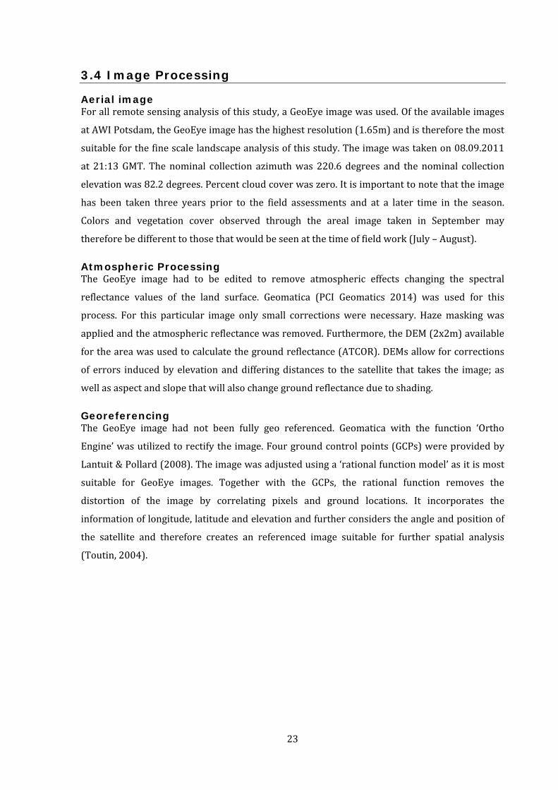
Aerial image Forallremotesensinganalysisofthisstudy,aGeoEyeimagewasused.Oftheavailableimages

atAWIPotsdam,theGeoEyeimagehasthehighestresolution(1.65m)andisthereforethemost

suitableforthefinescalelandscapeanalysisofthisstudy.Theimagewastakenon08.09.2011

at 21:13GMT.Thenominal collection azimuthwas220.6 degrees and thenominal collection

elevationwas82.2degrees.Percentcloudcoverwaszero.Itisimportanttonotethattheimage

has been taken three years prior to the field assessments and at a later time in the season.

Colors and vegetation cover observed through the areal image taken in September may

thereforebedifferenttothosethatwouldbeseenatthetimeoffieldwork(July–August).

Atmospheric Processing The GeoEye image had to be edited to remove atmospheric effects changing the spectral

reflectance values of the land surface. Geomatica (PCI Geomatics 2014) was used for this

process. For this particular image only small correctionswere necessary. Hazemaskingwas

appliedandtheatmosphericreflectancewasremoved.Furthermore,theDEM(2x2m)available

fortheareawasusedtocalculatethegroundreflectance(ATCOR).DEMsallowforcorrections

of errors inducedbyelevationanddifferingdistances to the satellite that takes the image; as

wellasaspectandslopethatwillalsochangegroundreflectanceduetoshading.

Georeferencing The GeoEye image had not been fully geo referenced. Geomatica with the function ‘Ortho

Engine’wasutilizedtorectifytheimage.Fourgroundcontrolpoints(GCPs)wereprovidedby

Lantuit&Pollard(2008).Theimagewasadjustedusinga‘rationalfunctionmodel’asitismost

suitable for GeoEye images. Together with the GCPs, the rational function removes the

distortion of the image by correlating pixels and ground locations. It incorporates the

informationoflongitude,latitudeandelevationandfurtherconsiderstheangleandpositionof

the satellite and therefore creates an referenced image suitable for further spatial analysis

(Toutin,2004).

24

3.5 Remote Sensing

Training Units Training units were created to link land cover units with spectral information. The training

unitswerecomprisedofthe23samplinglocations.Aroundeachsamplinglocationa10mcircle

was drawn in ArcGIS to create a polygon that covers the area around the point. Because

vegetationplotswereonly taken in threecardinaldirectionsaway fromthesamplingpoint,a

triangleinthemissingdirectionwascutoutfromthepolygon.Waterandwetpolygonalterrain

present in the study areawere not capturedwithin the 23 sampling locations and polygons

wereaddedbyhandtoincludethemastrainingunits.

Spectral Classification ThesoftwareENVI5.2.1wasusedtocombinetheDEMandGeoEye imagetocreatea totalof

fivespectralbandsthatwouldbeusedforcapturingtheremotesensingclasses.Theresolution

adjusted to layer with the lowest one (DEM ‐ 2m). At first, an unclassified remote sensing

methodwas tried.Themethoddoesnot require trainingunitsbut splits thearea intoclasses

basedondifferenceinspectralreflectance.Thenumberofclassescanbespecifiedandranged

from12to20inthisstudy.Thedifferentclassificationsystemstriedwiththeecologicalclasses

were parallelpiped,minimumdistance andmaximum likelihood. Suitability of thesemethods

wasevaluatedwithhelpofpicturesandexperiencedresearchersfamiliarwiththestudyarea.

Further, single random points were excluded from the classification and compared with the

remote sensing results. The classification system thatworked best for ecological classeswas

thenalsoappliedforthevegetationclasses.

Post Processing TheresultinglandcoverclassificationwasexportedfromENVItoArcGIStoeditthedata.Small

patches with differing classification were removed using focal statistics, keeping the most

commonunit (mode)within the four next neighbouring cells. Further, a boundary cleanwas

appliedtoremovekinksandirregularitiesuncommoninnature.Thesamemethodwasapplied

forbothecologicalandvegetationclasses.

Ground Truthing Usageofgroundtruthingpointsisagoodmethodtoverifytheaccuracyoftheremotesensing

technique.Thesepointsareadditionaldatapointswhereecologicalandvegetationclassesare

captured but have not been used in the remote sensing process. In this study, the ground

truthingpointscollected in2015wereoverlainwiththeremotesensingmapandbothvalues

wereextractedusingArcGIS.Therefore, foreachground truthingpoint there isanassociated

predictedandobservedvalue.

25

3.6 Laboratory Methods

Allsoilsampleswerefreezedriedfortwotofourdays.Dryweightwasmeasuredafterwardsto

calculatedrybulkdensityandwatercontent.Then,thesamplewassplitforfurtherpreparation

andanalysis.Anuntreatedsubsample(50g)wastakenandwillbeusedforgrainsizeanalysis

for furtherresearchprojectswithinAWIPotsdam.Asecondsubsample(12ml)wasmilledat

360 rpm for eight minutes in order to homogenize the substrate for precise chemical

assessmentsandwasusedfortotalcarbon(TC),nitrogen(TN)andtotalorganiccarbon(TOC)

measurements.

Dry Bulk Density and Water Content Bulkdensityisanimportantmeasurementtocharacterizethesoil.Itcanvarygreatlywithgrain

size, land use or biological and geological processes. Bulk density is needed to translate

percentagenutrientcontentsintodensities(weightpervolume).Soilbulkdensitiesrangefrom

0.3g/cminorganicsoilsand1.0g/cm(finetexturedsoils)to1.7g/cm(coarsetexturedsoils)

(Brady&Weil,1996).Bulkdensitywascalculatedasfollows:

/

Thegravimetricwatercontentgivesanindicationaboutsoilmoistureatthetimeofsampling.It

can also give an indication about the kind of vegetation and landscape dynamics that can be

expected(Oecheletal.,1993).Itwascalculatedasfollows:

100

%

Grain Size Distribution A50gramsubsamplewaswetsievedwithameshsizeof1mmwhichseparatedthegrainsinto

coarse(verycoarsesandandlarger)andfine(lessthan1mm).Thecoarsefragmentwasdried

at60Cfortwodaysandthefinefragmentwasdriedinadryfreezerfortwodays.Thecoarse

fragment was weighed and percentages of the fragment were calculated using the total dry

weight.

26

Total Carbon, Nitrogen and Total Organic Carbon Part of the homogenized soil sample was used for carbon and nitrogen (CN) analysis. Two

replicatesof5mgwereweighedintotinboats.Soilsamplesaswellasstandardsubstancesused

asreferencepoints,weremeasuredwithanelementanalyzer(ElementarvarioELIII).

This analyzer works throughmeans of catalytic combustion where carbon and nitrogen are

oxidized at high temperatures and turned into their gaseous phases. Themolecules are then

separated by adsorption columns and measured by a thermal conductivity detector. The

percentcarbonandnitrogenarethencalculatedfromthedifferenceofthetotalsampleweight

used for combustion. For the total organic carbon (TOC) measurements, 20‐100mg of

homogenizedsamplewasweighedintosmallcrucibles.Totalorganiccarbonismeasuredina

similar way to total carbon and nitrogen, only that combustion temperatures are lower,

preventingnonorganiccarbontoenterintothegaseousphase.Emptycontainerswereusedto

detect background noise, which is subtracted from the overall percentages. Furthermore,

standardswithknowncarbonandnitrogenvalueswerefittedwiththemeasuredpercentages

tocorrectforpotentialoverorunderestimationofmeasuredvaluesoneachday.Theamountof

TOC and TN were measured as percentages. Information about soil density then helped to

convertpercentagesintoTOCandTNstorage(kg/m²)withinthesoil:

%10

/

/ % (%)

%10

/

/ % (%)

27

3.7 Data Processing and Analysis

AlldatawasorganizedandmaintainedinExceldatabases(Office2010),statisticalanalysesand

figureswerecodedinR3.1.1.SpatialdatawasstoredatprocessesinArcGIS11.3(ESRI).

Location Properties Somelocationpropertieswerenotobtainedthroughfieldworkbutinstead,usingremote

sensingmethods.SlopewascalculatedusingtheDEM.Thedistanceofsamplinglocationstothe

nearestcreekwasextractedusingaflowdirectionraster.Thenormalizeddifferencevegetation

index(NDVI)wascalculatedusingtheprogrammeENVI.TheNDVIdescribestheproportionof

thevegetationthatisbiologicallyactiveandcangiveanindicationofdifferentplant

communitiesandforsmallareasalsothepheonolgicalstageswithintheseason.Itiscalculated

astherelativestrengthofredtonearinfrared(NIR)lightwithinagivenarea.

TheDEMwasusedtocalculatethetopographicwetnessindex(TWI)whichusesslopeto

estimatewateraccumulationsites.Itiscalculatedasfollows

ln

α=cumulativeupslopeareadrainingthroughapointβ=slopeangleatthatpoint

BothNDVIandTWIhadalreadybeencalculatedforthesameprojectareaandweretherefore

notredoneforthisreport.

28

Soil Characteristics Ateachlocationsamplesweretakenatdifferentdepthsandhadtobeconvertedintoasingle

valuerepresentingtheoverallsoilqualityateachlocation.Formostcharacteristics,solelythe

valueofthetopmostcorewastaken(conductivity,pH,moisture,bulkdensityandpercentageof

coarse fragments). TOC and TN (kg/m²) contents of soil in between sampling depths were

extrapolated to the equal distance between them. TOC and TN values (kg/m²) where then

determined by adding the extrapolated measurements to the depths of 30 cm (global

comparisonstandard)andthelimitoftheactivelayer.Theywillsometimesbeabbreviatedto

TOC/TN‐30cmandTOC/TN‐active.TheCNratiowascalculatedastheproportionofTOCtoTN.

In this thesis it is referred toasCNandvalues in figuresaredisplayedas the fractionofTOC

overTN(TOC/TN).

Vegetation Data The vegetation data was processed for analysis in three ways. First, using the vegetation

percentagecoverandwiththeaidofpictures,vegetationclasseswereassignedaccordingtothe

descriptionsofSmithetal.(1989).Second, forcommunityanalyses,onlyrecordsof forbsand

shrubswereused (feces, litter,moss cover etc.were removed).And third, forNMDSanalysis

plotswithnovegetationcoverwereremovedandforPCAanalysisallthreeplotsatonelocation

wereaddedtogether.

Boxplots for Ecological and Vegetation Classes and Watershed Becausesamplesizeswithinclasses, thevariationofTOC,TN,CNratioandactive layerdepth

weredisplayedusingsimpleboxplots.Onesetofboxplotswascreatedwithecologicalclasses

and,forcomparison;thesamesettingswereusedforvegetationclasses.Furthermoreallvalues

fromeachtransectweregroupedtogetherandcomparedviaboxplots.

NMDS NMDS is short for non‐metric multidimensional scaling. It uses ranks of similarity or

dissimilaritytogroupsamplinglocationswithmoresimilarcharacteristicsclosertogether.Itis

amultidimensional approachbut isusuallydisplayedas a twodimensional graph.The stress

indicateshowwell thedatawasfitted intothegivendimensions.Avalueof0.3 indicatesthat

thearrangementisarbitrary,0.05wouldbeagoodfit.Statisticaltests,likesimperanalysis,can

quantifytheuniquenessofdifferentsamplinggroups.Forthisstudy,anNMDSwaschosenasan

alternativemethod to avoid the reducing diverse plant communities into simple classes that

wouldhavebeennecessarytocreateboxplots.Eachvegetationplotwastakenasaseparateunit

(n=66)andpercentagecoverswereusedtocomparethecommunitystructures.Theresulting

pointsinordinationspacewerelabelledtowhichecologicalclasstheybelong.Thisallowsfora

qualitative assessment, on how well differences in plant communities align with ecological

classes.

29

PCA PCA is short for principal component analysis which is a statistical method to analyze

correlations ofmultiple variables together and place them in amultidimensional space. It is

usually displayed in a two dimensional grid where the first and second axis are the ones

explainingmostofthevariationwithinthedata.Samplinglocationswithsimilarcharacteristics

willbeplacedclosertogether.Vectorsrepresentingthefactorsarefittedwithintheordination

space.Theycangiveinformationaboutredundancyamongvariablesiftheyareorientedinthe

same direction. Further, the direction and strength of the vectors gives an indication which

factorsareimportantatexplainingthedifferentcharacteristicsbetweensamplingpoints.

Forthisstudy,thefollowingsoilandlocationcharacteristicswereincludedinthePCA: active

layer depth, organic horizon depth, bulk density, coarse fragment percentage, moisture,

percentageofbaregroundandlitter,slope,NDVI,distancetothecreek,TOC,TN,CNratiowithin

thefirst30cmandtheentireactivelayer.ThesitecharacteristicsvectorsinlinewiththeTOC

andTNvectorswouldshowthehighestco‐correlationandbestdescribethevariationofcarbon

andnitrogenintheactivelayerofthesoil.Theecologicalandvegetationclasseswereaddedto

the plot and close grouping of all points from one class indicates that it has distinct soil

characteristicssuchashighestmoisture,intermediateNDVIandlowpercentageofopenground.

Landcover Comparisons LandcoverclassificationsforecologicalandvegetationclasseswerecomparedinArcMap11.3

(ESRI)byusingthezonalstatisticstooltocreateatableindicatingwhatpercentageofareaeach

classshares.ByclippingtheIceCreekwatershedbyitsEastandWestsectionsthetotalareaof

ecological and vegetation class within each area could be calculated and converted into

percentages.

Further Statistical Analysis ANOVAs in connection with Tukey HSD post hoc test were carried out to detect significant

differencesbetweendifferentdatasets.Pvaluesof<0.1wereconsideredsignificantduetosmall

sample sizes and heterogeneous ecological data. However, all p values stated in this thesis

shouldonlybetakenasorientationtodetectlikelydifferencesbecausesamplesizesweresmall

and not normally distributed. Non‐categorical data was assessed with the Spearman’s rank

correlation testwhich is a goodmethod for small datasets that are not normally distributed

(Gauthier,2001).

30

4. Results

4.1 Remote sensing

Classification System Themaximumlikelihoodclassificationmethod(supervisedclassification)wasselectedtomap

the ecological and vegetation classes. This most was deemedmost suitable, based on visual

assessments and evaluation of the classes with randomly chosen ground truthing points.

Parallelpipedandminimumdistancemethodscreatedclassificationsthathadverysharpedges

unusualfornaturalsystemsandwerethereforenolongerconsideredinthisstudy.

Ecological and Vegetation Classes The remote sensing outputs for ecological classes were similar to the ones for vegetation

classes.Typically,foreachecologicalclass,therewasavegetationclassassociatedwithit(table

2).However,thisdoesnotnecessarilymeanthatacertainvegetationtypewillbefoundinan

ecological zone. Figures 5 and 6 underlay the similarities and differences found in the

distributionofbothecologicalandvegetationclasses.

Table2:Associationofvegetationtypestoecologicalclasses.Eachcolumnshowstowhatpercentageacertainvegetationtypecanbefoundwithintheecologicalclass.

Vegetation class /  Ecological class  

(correspondence in percent)  Herschel Herschel‐Komakuk  Komakuk 

Plover‐Jaeger 

Wet Terrain  Thrasher 

Shrub Zone 

Cottongrass/Moss  99.5  76.6  12.8  7.4  13.4  0.1  0.0 

Arctic Willow/Dryas Vetch  0.0  21.5  82.7  1.2  0.4  1.4  0.4 

Willow/Saxifrage‐Coltsfoot  0.4  0.0  0.3  0.6  84.1  5.9  6.0 

Arctic Willow/Lupine‐Forget‐me‐not  0.0  1.8  3.1  84.9  0.7  11.2  2.7 

Grass/Chamomille‐Wormwood  0.0  0.1  1.1  5.6  0.3  73.9  0.0 

Shrub Zone  0.0  0.0  0.1  0.3  1.2  7.5  90.9 

Total  100  100  100  100  100  100  100 

31

00.

5 Km

00.

5 Km

¯¯

Ec

olo

gic

al

Cla

sses

He

rsch

el

He

rsch

el-

Ko

ma

kuk

Ko

ma

kuk

Plo

verJ

ae

ge

r

Sh

rub

Zo

ne

Th

rash

er

Wet

Te

rrai

n

Gu

ille

mo

t

Veg

eta

tio

n C

las

ses

Co

tton

gra

ss/M

oss

Arc

tic W

illow

/Dry

as

Ve

tch

Will

ow

/Sa

xifr

ag

e-C

olts

foo

t

Arc

tic W

illow

/Lup

ine

-Fo

rge

t-m

e-n

ot

Gra

ss/C

ha

mo

mill

e

Sh

rub

Zo

ne

Po

lyg

on

al W

etla

nd

Figure11:ClassificationoftheIceCreekwatershedusingecologicalunits(left)andvegetationunits(right).

32

1

0 0,5Km

3

2

¯

Figure 12: Highlights of study area where the vegetation type does not coincide with the typicallyassociatedecologicalclass.Intheextents1)and2)EriophorumextentsfurtherintothesteepersectionsofthewatershedthanwouldbesuggestedbytheHerschelecologicalclass.In3)moreareasarecoveredbythegrass‐chamomilevegetationclassaswouldbepredictedbytheextentoftheThrasherunit.

0 150m

3a 3b

0 150m

0 150m

0 150m

b) Vegetation Classes

Cottongrass/Moss

Arctic Willow/DryasVetch

Willow/Saxifrage-Coltsfoot

Arctic Willow/Lupine-Forget-me-not

Shrub Zone

Grass/Chamomille

a) Ecological Classes

Herschel

Herschel-Komakuk

Komakuk

Wet Terrain

Plover-Jaeger

Shrub Zone

Thrasher

1a 1b

2a 2b

¯ ¯

¯ ¯

¯ ¯

0 150m

0 150m

33

Ground Truthing The ground truthing tables compare to what extent predicted classes coincide with field

observations.Forboththeecologicalaswellasthevegetationclasses,thepredictionaccuracy

varied between 0‐100% and 25‐100% respectively. Neither classification system had a

considerablyhigherpredictionaccuracy.Thetotalgroundtruthingaccuracyfortheecological

zones was 55% and 45% for vegetation classes. The classes Herschel and Thrasher had a

predictionaccuracyof100%.Thrasherwasfoundinthefieldinareaswhereitwasnotdetected

bytheremotesensingprocessandthereforetheobserver’saccuracyislower.Twothirdsofthe

areapredictedtobecoveredbyKomakukwerecoveredwithPlover‐Jaegerinstead. Inversely,

areas thatwere found tobeKomakukwerepredicted tobeWetTerrainandShrubZone.For

moreinformation,seetable3.

The vegetation classes showed a similar pattern as ecological classes. The grass‐chamomile

vegetationclasshadapredictionaccuracyof100%.Eriophorum,usuallyastrong indicatorof

the Herschel ecological class, only had a prediction accuracy of 50%. Arctic Willow/Lupine‐

Forget‐me‐not areas were predicted to an accuracy of 60% but observer’s accuracy is

considerably lowerbecause thevegetationclasswas found inmoreareas thanpredicted.For

moreinformation,seetable4.

Table 3: Classification accuracy between observed (ground truthing) and predicted (classification)ecologicalunits.

predicted/ observed  Herschel  Komakuk 

Herschel‐Komakuk 

Plover‐Jaeger 

Wet Terrain 

Shrub Zone  Thrasher 

Predictor's accuracy 

Herschel  2  100% 

Komakuk  1  2  33% 

Herschel‐Komakuk   

1  

0% 

Plover‐Jaeger  1  4  1  67% 

Wet Terrain  1  1  50% 

Shrub Zone  1  1  1  33% 

Thrasher  2  100% 

Observer's accuracy 

100%  33%  0%  57%  50%  100%  67% 

34

Table 4: Classification accuracy between observed (ground truthing) and predicted (classification)vegetationunits.

predicted/ observed 

Cottongrass/Moss 

Arctic Willow/ Dryas Vetch 

Willow/Saxifrage‐Coltsfoot 

Arctic Willow/Lupine‐Forget‐me‐

not Grass/ 

Chamomile Shrub Zone 

Predictor's accuracy 

Cottongrass/ Moss 

2  2  50% 

Arctic Willow/Dryas Vetch 

1  2  33% 

Willow/Saxifrage‐Coltsfoot 

1  1  50% 

Arctic Willow /Lupine‐Forget‐me‐not 

1  1  3  60% 

Grass/ Chamomile 

3  100% 

Shrub Zone 

1  1  1  33% 

Observer's accuracy 

67%  25%  50%  43%  100%  100% 

35

4.2 Ordination

NMDS Plantcommunitiesandnotvegetationclassessuchastheonesreportedonin4.1)didnotalign

as clearly with the ecological classes as vegetation classes do (figure 13). The Herschel unit

appearedtobeaverydistinctplantcommunity.However,thePlover‐Jaegerunitencompassed

vegetation communities that were very dissimilar and were not to be separated from the

Komakuk andmost Thrasher points. TheWet Terrain and Shrub areas also overlappedwith

theirplantcommunities.

Figure 13:Non‐metricmultidimensional scaling (NMDS) of forbs and shrubs at 66 sampling locations.Correspondencewithecologicalzonesisindicatedbysymbolsandcolours.Stress:0.176.HEHerschel,HKHerschel‐Komakuk,KOKomakuk,PJPlover‐Jaeger,SZShrubZone,THThrasher,WTWetTerrain.

Axis1

Axi

s2

Type

HE

HK

KO

PJ

SZ

TH

WT

36

PCA ThePCA included severalparameters includingTOC, TN andother soil properties.ThePCA

outputs reflecteda similarpicture as theboxplots.Ecological classeswerenotbetterdefined

than vegetation classes. Neither method created distinct groups that show no overlap with

others.Plover‐JaegerhadsoilpropertiessimilartoThrasherwhiletheHerschel,Komakuk,and

Wet Terrain units all had similar soil properties. The Camomile and Salix‐Lupine vegetation

classesbothformeddistinctgroupsandweredefinedbyadeepactivelayer,highbulkdensity

and a high percentage of bare ground. The other vegetation classes could not be clearly

separated fromoneanother (figure15).ThePCAalsoshowedthatCNratiosclosely followed

the samedirection asNDVI and the depth of the organic horizon. Additionally, TOC down to

30cmwaspositively correlated to topsoilmoistureandnegatively correlated tobulkdensity,

active layer depth and percentage of bare ground. TN‐30cm and TOC‐active showed less

alignmentwithanyof investigated soilproperties.TN‐activewasnegatively correlated to the

percentageofcoarsegrainsandslope.

37

Figure14:Principalcomponentanalysisofsoilpropertiesat23samplinglocationswithecologicalclassesindicated in different colours. HE Herschel, HK Herschel‐Komakuk, KO Komakuk, PJ Plover‐Jaeger, SZShrubZone,THThrasher,WTWetTerrain.

Figure 15: Principal component analysis of soil properties at 23 sampling locations with vegetationclassesindicatedindifferentcolours.

depth

bareground

depth_organic

moisturebulk_density

grain_coarse

TOC_active

TN_30cm

TN_active

dist

ance

_str

eam

slope

NDVI

litte

r−3

−2

−1

0

1

2

−5.0 −2.5 0.0 2.5 5.0PC1 (53.6% explained var.)

PC2

(10.

8%ex

plai

ned

var.)

groups

HE

HK

KO

PJ

SZ

TH

WT

CN_30TOC_30cm

CN_active

depth

bareground

depth_organic

moisture bulk_density

grain_coarse

TOC_30cm

TOC_active

TN_30cm

TN_active

dist

ance

_str

eam

slopeNDVI

litte

r

CN_30

CN_active

−5.0

−2.5

0.0

2.5

−2.5 0.0 2.5 5.0PC1 (53.6% explained var.)

PC2

(10.

8%ex

plai

ned

var.)

groups

Camomille

Dryas

Eriophorum

Petasites

Salix−Lupine

Shrub

38

4.3 Ice Creek Total Organic Carbon and Nitrogen Storage

Terrain Generally,Spearman’srankcorrelationswere thehighest formoisture, followedbyNDVIand

slope.TWIwasnotwellcorrelatedtoTOCandTN.CorrelationswithTNcontentsintheactive

layerasawholewerenotsignificantforallcomparedparameters.

Table5:Spearman’srankcorrelation(ρ)ofTWI(topographicwetnessindex),moistureintopsoil,NDVI(normalized difference vegetation index) and slope (in degrees) with TOC (total organic carbon), TN(totalnitrogen)andtheCNratio.Significanceof<0.1=*and<0.05=**.

ρ  TOC 0‐30cm  TOC Active  TN 0‐30cm TN Active CN 0‐30cm CN Active 

moisture  0.74**  0.61**  0.65**  0.31  0.84**  0.73** 

TWI  0.36*  0.37*  0.22  0.25  0.4*  0.44** 

slope  ‐0.44**  ‐0.42**  ‐0.35*  ‐0.21  ‐0.43**  ‐0.5** 

NDVI  0.48**  0.46**  0.54*  0.23  0.55**  0.5** 

Ecological Classes Totalorganiccarbon(TOC)wasnotevenlydistributedthroughoutthewatershed.Slopedareas

with high shrub densities (Shrub Zone) held the highest amounts of TOC. Theywere closely

followedbyflatuphillareas(HerschelZone).ThedifferencesinTOCwithinthefirst30cmofthe

soilwerenotaspronouncedcomparedtotheentireactivelayerdepth.ThelowestTOCvalues

werefoundinrecentlydisturbedareas(Thrasher).ThedistributionofTOCandnitrogenwere

similarandhighlycorrelated(r=0.95,p=9.927e‐12,df=21).CNratioswerethelargestwithin

the Herschel Zone, followed by shrub areas. The Thrasher zones had the smallest ratio. The

KomakukandPlover‐Jaegerzoneswerecharacterizedbysoilcarbonandnitrogencontentsthat

are intermediate compared to the zones described above, The Komakuk Zone, however.

generallyhadhigherTOCandnitrogencontentsaswellasashalloweractive layerdepth.For

detailedinformation,seefigures16and17aswellastable6.

39

00.

5 Km

00.

5 Km

¯¯

Tota

l Org

an

ic C

arb

on

0-3

0 cm

(k

g/m

²)<

5.0

<1

0.0

<1

5.0

Tota

l O

rgan

ic C

arb

on

Ac

tiv

e L

ay

er

(kg

/m²)

<5

.0

<1

0.0

<1

5.0

<2

0.0

<2

5.0

Figure16:Totalorganiccarbon(kg/m²)at0‐30cm(left)andtheentireextentoftheactivelayer(right)inIceCreekwatershedonHerschelIsland.

40

00.

5 Km

00.

5 Km

¯¯

Tota

l Nit

rog

en

0-30

cm

(k

g/m

²)<

0.2

5

<0

.50

<0

.75

<1

.00

<1

.25

Tota

l N

itro

ge

n

Ac

tiv

e L

ay

er (

kg

/m²)

<0.

25

<0.

50

<0.

75

<1.

00

<1.

25

<1.

50

<1.

75

<2.

00

Figure17:Totalnitrogen(kg/m²)at0‐30cm(left)andtheentireextentoftheactivelayer(right)inIceCreekwatershedonHerschelIsland.

41

Ecological Class 

Active Layer  

Dep

th (cm

) Bulk Den

sity  

(g/m

³) 

Moisture 

 (%) 

TOC‐30cm

  (kg/m

²) 

TOC‐active 

 (kg/m

²) 

TN‐30cm

  (kg/m

²) 

TN‐active 

 (kg/m

²) 

CN‐30cm

  (kg/m

²) 

CN‐active 

 (kg/m

²) 

Bareground 

 cover (%

) Slope (°) 

NDVI 

TWI 

Herschel 

35 

0.52 

56.60 

11.91 

13.96 

0.88 

1.05 

13.66 

13.44 

0.00 

4.53 

0.70 

8.98 

Herschel‐Komakuk 

48 

1.07 

26.90 

7.85 

24.71 

0.74 

1.88 

10.60 

13.12 

0.75 

4.73 

0.67 

8.05 

Komakuk 

52 

0.72 

40.93 

8.22 

12.75 

0.81 

1.38 

9.99 

9.08 

0.35 

5.58 

0.66 

7.88 

Plover‐Jaeger 

74 

1.36 

14.88 

4.39 

6.07 

0.56 

0.92 

6.27 

5.79 

69.50 

10.64 

0.62 

7.96 

Shrub Zone 

59 

0.36 

62.90 

13.51 

21.68 

1.08 

1.89 

12.47 

11.49 

0.00 

6.52 

0.68 

9.05 

Thrasher 

73 

1.38 

11.85 

1.72 

4.30 

0.35 

0.87 

4.49 

4.43 

97.75 

15.78 

0.58 

7.93 

Wet Terrain 

50 

0.86 

38.22 

9.17 

13.12 

0.91 

1.38 

9.82 

9.45 

5.03 

9.16 

0.76 

8.39 

Table6:Averagesofsoilandlandscapepropertiesforeachecologicalclass.Carbonandnitrogencontentsarehighestforthe

ShrubZoneandlowestforThrasherareas.BulkdensityofthetopsoilishighestforPlover‐JaegerandThrasherandlowestfor

theHerschelclass.Asimilartrendcanbedetectedfortopsoilm

oisture.Furtherinformationaboutactivelayerdepth,

moisture,density,TOC,TN,CN,percentageofbareground,slope,NDVIandTWIcanbeobtainedfrom

thetable.

42

IceCreekEastandWestweresimilarinsizeandoveralldistributionofvegetation.theHerschel

ecologicalclasscoveragewasgreater in IceCreekWest. In IceCreekEast,greaterareaswere

coveredbytheKomakukandPlover‐Jaegerclasses.Totalstorageofcarbonintheactivelayerin

IceCreekWestwas15999tonnesand17392tonnesforIceCreekEast.StorageofNitrogenwas

1673and1962tonnesrespectively.Together,bothwatershedsheld22978tTOCinthefirst30

cmand33391tintheactivelayer.Nitrogenstoragewas2256tdownto30cmand3635tinthe

entireactivelayer.Fordetailedinformation,seetable7.

Table7:Comparisonof area coveredby ecological classesandTOC,TN storage in IceCreekWest andEast.

  Ice Creek West Ice Creek East 

Ecological Class 

Percentage 

cover 

TOC‐30cm (tonnes

) 

TOC‐active (tonnes

) 

TN‐30cm (tonnes

) 

TN‐active (tonnes

) 

Percentage 

cover 

TOC‐30cm (tonnes

) 

TOC‐active (tonnes

) 

TN‐30cm (tonnes

) 

TN‐active (tonnes

) 

Guillemot  0.1    ‐    

Herschel  20.6  3435  4027 253 302 4.1 781  916  57 69

Herschel‐Komakuk 

 0.6  66  208  6  16   0.8  100  316  9  24 

Komakuk  24.4  2807  4354 276 472 37.5 4931  7648  484 830

Plover‐Jaeger  29.0  1781  2463 229 375 35.6 2498  3455  321 527

Shrub Zone  5.6  1060  1700 85 148 6.4 1384  2220  111 193

Thrasher  3.0  72  181 15 36 3.1 85  213  18 43

Wet Terrain  16.7  2143  3067 212 324 12.5 1834  2623  181 277

Total    11364  15999 1075 1673 11614  17392  1181 1962

Upon visual inspection of the boxplots, neither the ecological nor the vegetation approach

dividedTOCorTNvaluesintowell‐definedclasses.FortheTOCvalues,therewasahigherin‐

class variance found in the vegetation classes.This variationwashowever, consistent for the

TOC‐30cmandTOC‐activevalues.AsidefortheWetTerrain,theecologicalclassesatTOC‐30cm

createdquitedistinctgroupsbut includedmoreoutliersthanthevegetationclasses.Onevery

highTOCvalue inthePlover‐Jaegersectionchangedthevarianceandaverageof thisecoclass

greatly.TheHerschel‐Komakukclasswasnot consistent in theTOC‐30cmand theTOC‐active

layer.Inthefirst30cm,thevaluewascomparabletotheKomakukclass,whereasattheentire

activelayerdepth,TOCvalueswereevenhigherthanthosefoundintheshrubzone.Thehigh

carboncontentcanbeexplainedbyapeatylayerfoundat40cmdepth.Duetothesmallsample

size(n=1),thereisnooptiontovalidateiftheHerschel‐Komakuktypeisusuallyunderlainby

peatandifthesampleanalyzedhereisrepresentativeornot.ThespreadofTNwassimilarto

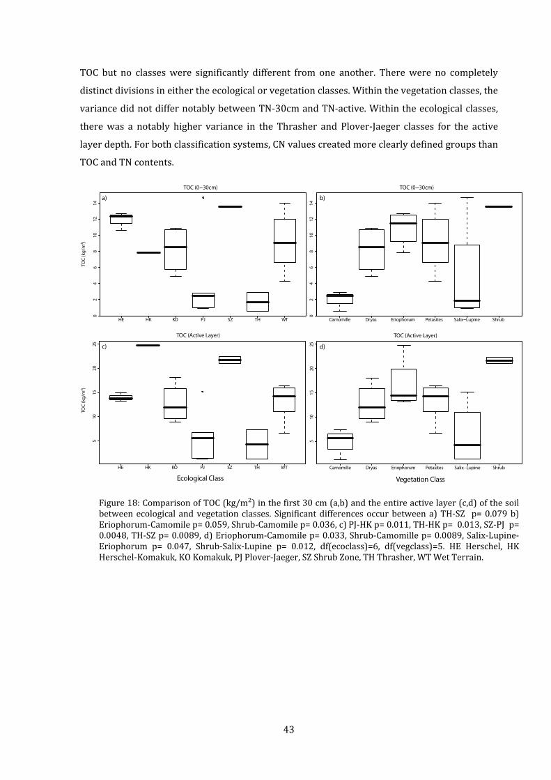
43

TOC but no classeswere significantly different from one another. Therewere no completely

distinctdivisionsineithertheecologicalorvegetationclasses.Withinthevegetationclasses,the

variancedidnotdiffernotablybetweenTN‐30cmandTN‐active.Withintheecologicalclasses,

therewas a notably higher variance in the Thrasher and Plover‐Jaeger classes for the active

layerdepth.Forbothclassificationsystems,CNvaluescreatedmoreclearlydefinedgroupsthan

TOCandTNcontents.

HE HK KO PJ SZ TH WT

02

46

810

1214

TOC (0 30cm)

HE HK KO PJ SZ TH WT

510

1520

25

TOC (Active Layer)

Ecological Class

TOC

(kg/

m²)

TOC

(kg/

m²)

Camomille Dryas Eriophorum Petasites Salix Lupine Shrub

510

1520

25

TOC (Active Layer)

Vegetation Class

Camomille Dryas Eriophorum Petasites Salix Lupine Shrub

02

46

810

1214

TOC (0 30cm)

a)

c)

b)

d)

Figure18:ComparisonofTOC(kg/m²)inthefirst30cm(a,b)andtheentireactivelayer(c,d)ofthesoilbetweenecological andvegetation classes. Significantdifferencesoccurbetweena)TH‐SZ p=0.079b)Eriophorum‐Camomilep=0.059,Shrub‐Camomilep=0.036,c)PJ‐HKp=0.011,TH‐HKp=0.013,SZ‐PJp=0.0048,TH‐SZp=0.0089,d)Eriophorum‐Camomilep=0.033,Shrub‐Camomillep=0.0089,Salix‐Lupine‐Eriophorum p= 0.047, Shrub‐Salix‐Lupine p= 0.012, df(ecoclass)=6, df(vegclass)=5. HE Herschel, HKHerschel‐Komakuk,KOKomakuk,PJPlover‐Jaeger,SZShrubZone,THThrasher,WTWetTerrain.

44

HE HK KO PJ SZ TH WT

0.2

0.4

0.6

0.8

1.0

1.2

1.4

TN (0 30cm)

Camomille Dryas Eriophorum Petasites Salix Lupine Shrub

0.2

0.4

0.6

0.8

1.0

1.2

1.4

TN (0 30cm)

HE HK KO PJ SZ TH WT

0.5

1.0

1.5

2.0

TN (Active Layer)

Ecological ClassCamomille Dryas Eriophorum Petasites Salix Lupine Shr

0.5

1.0

1.5

2.0

TN (Active Layer)

Vegetation Class

ub

TN(k

g/m

²)TN

(kg/

m²)

a)

c)

b)

d)

Figure19:ComparisonofTN(kg/m²)inthefirst30cm(a,b,)andtheentireactivelayer(c,d)ofthesoilbetween ecological and vegetation classes. No significant differences occur between the differentecologicalorvegetationclasses.HEHerschel,HKHerschel‐Komakuk,KOKomakuk,PJPlover‐Jaeger,SZShrubZone,THThrasher,WTWetTerrain.

45

HE HK KO PJ SZ TH WT

4050

6070

80

Active Layer Depth

Ecological Class

Camomille Dryas Eriophorum Petasites Salix Lupine Shrub

4050

6070

80

Active Layer Depth

Vegetation Class

CNR

atio

Dep

th(c

m)b

elow

surf

ace

e) f )

Camomille Dryas Eriopherum Petasites Salix Lupine Shrub

46

810

1214

CN Ratio (0 30cm)

Camomille Dryas Eriopherum Petasites Salix Lupine Shrub

46

810

1214

CN Ratio (Active Layer)

HE HK KO PJ SZ TH WT

46

810

1214

CN Ratio (0 30cm)

HE HK KO PJ SZ TH WT

46

810

1214

CN Ratio (Active Layer)

a) b)

c) d)

CNRa

tioa

ab a

a

a

b

b

a

ab

a

ab

c

b

bc

aa

bc

b

b

c c

c

abc

bc ac bc

aab

d

bc

a

b

ab

cd

a

b

b

b ab

a

Figure20:ComparisonofCNratiosinthefirst30cm(a,b,)andtheentireactivelayer(c,d)ofthesoil aswellasactivelayerdepth(e,f)betweenecologicalandvegetationclasses.Significantdifferences(p=0.1)areindicatedbydifferentlettersbesideseachplot.HEHerschel,HKHerschel‐Komakuk,KOKomakuk,PJPlover‐Jaeger,SZShrubZone,THThrasher,WTWetTerrain.

46

TransectsFigure21illustratesthedistributionofTOCcontentswithinthethreetransectssurveyedinthe

field.For informationabout theexactpositionsof the transects, referbackto figure10 in the

methods.

Intheuppertransect,thecreekdidnotformaverydeepincisionandslopesweregentle.The

amountofcarbonpresent in thesoildidnotvarymuchbetweendifferentcatenarypositions.

Totalactivelayerdepth,incomparisontothefirst30cm,didnotaddconsiderablymorecarbon.

Thiscanmainlybeattributedtoshallowactivelayerdepths.Thegeneralpatterninthemiddle

andlowerwatershedwasthathighelevationsiteshadhighTOCcontentinthefirst30cmbut

similartotheuppertransect locations,active layerdepthwasshallowandTOC‐activedidnot

add much carbon. In locations that were not on the flat uplands, the soil below 30 cm

contributed at least as much carbon as the first 30 cm. There was no linear trend of TOC

contents decreasing toward the stream. Instead, high upland TOC contentswere followed by

lowervaluesonslopesandincreasedagaininproximitytothestream.Inthreelocations(onein

themiddle transect, two further downstream) TOC contentswere extremely low in both the

first30cmanddeeper.

47

Figure21:Totalorganiccarbon(kg/m²)ateachsamplingpointonthreetransectsacrosstheIceCreekwatershed.Histogramsinlightgrey:TOC(0‐30cm),indarkgrey(TOC‐active).Thelineindicatestheelevationofeachsamplinglocation.Distancesbetweenpointsonthexaxisarenottoscale.Additionalelevationsoutsideofsamplinglocationsarenotincluded,additionalridgesandvalleysmaythereforebeenoverlooked.TheuppertransectonlypassedthroughIceCreekWest.

48

Thesoil (0‐30cm) in theupperandmiddle transectsheldmoreTOCandTNcompared to the

transect in the lower reach of the watershed (fig. 22a,b). This difference was smaller, and

statistically not significant, when the entire active layer depth was taken into account.

Statistically significant differences were found for TOC (0‐30cm), p=0.065 (upper‐lower

transect) and TN (0‐30cm), p=0.051 (upper‐lower transect), df=22. CN values were much

greater for the upper areas of the watershed. The difference in CN ratios became more

pronounced ifonlysamplessitesdirectlysituatedbythestreamweretaken intoaccount(fig.

22d‐ CN Ratio Creek). Because of their discrete nature, however, TOC and TN boxplots for

stream adjacent sites are not shown in the figures. Significant differences for creek proximal

sites were found for TOC (0‐30cm), p=0.039 (upper‐lower transect), TN (0‐30cm), p=0.071

(upper‐lowertransect)andCN,p=0.063(upper‐lowertransect),df=9.

Figure22:BoxplotscomparingthedifferencesinTOC,TNandCNratiosbetweenanupper,middleandlowertransectwithintheIceCreekWatershed.

a) b)

c) d)

49

5. Discussion

Themain goal of this studywas to create a fine scalemapwithorganic carbon andnitrogen

estimatesforbothIceCreekwatersheds.Theobjectivewasalsotounderstandspatialpatterns

in thedistributionof soil organic carbonandnitrogen tohelp future studies thatwill lookat

fluvialdischargeandsediment flowswithin thewatershed.The first sectionof thediscussion

will evaluate the detectability of land cover classes and how well the classification systems

characterizethesoil.Thesecondpartwillinvestigatehowthespatialdistributionofsoilorganic

carbon and nitrogen is related to terrain. Information on terrain, ecological classes and the

transect‐basedinvestigationwillthenbebroughttogethertoassessactivelayercharacteristics

of the Ice Creekwatershed. Finally, the implications of the overall and spatial storage of soil

organiccarbonandnitrogenforpotentialfluxesoforganicmatterfromtheIceCreekintheface

ofachangingclimatewillbeaddressed.

50

5.1 Remote Sensing Classification

Detectability

MotiveAcommonapproachtoupscalingorganiccarbon(TOC)andnitrogen(TN)fromsinglesoilpits

to larger areas is by using land classification maps. Landscape classes chosen because they

explainsoilpropertieswellmay,however,notbeeasilyidentifiedthroughremotesensing(RS)

techniquesiftheclassesspectralimagepropertiesaretoosimilar.ThedefinedRSclasseswould

ideally require few training sets to reduce field work and be detected using different image

types.The idea is thattheclassesarespectrallydistinctenoughthat it ispossibletocorrectly

predicttheoccurrenceoftheseclassesinanunknown(sofarunclassified)area.Dependingon

thespreadandtheinformationbehindthedata,differentclassificationalgorithmsmightgroup

theclassesbest.Theexpectedpredictionaccuracywilldependgreatlyonthespatialresolution

oftheproject(McKenzie&Ryan,1999).

EvaluationInthisstudy,amaximumlikelihoodclassificationwasdeemedtobethemostsuitablemethod.

This method was compared to other ones and selected based on an accuracy assessment

conductedwithgroundtruthingpointscollectedinthefield,aswellasinputfromexperienced

researchers familiarwiththestudyarea.Maximumlikelihoodalsohastheadvantagetoallow

for comparisonswithotherRS carbonestimate studies (Hugelius et al., 2010;Hugelius et al.,

2012;Zubrzyckietal.,2013).Randomlyexcludingtrainingunitstousethemasgroundtruthing

pointsworkswellwhenthereareenoughtrainingunitsavailable.Butwhentherearetoofew,

importantinformationfortheclassificationwillbelacking.Findingthebalanceofanadequate

numberof trainingunitsandenoughvalidationpoints isacommondilemma formapmakers

(Young,2008).Atthetimeoftheconceptionoftheclassificationsystem,groundtruthingpoints

collected in summer 2015 were not available and this explains the limited use of ground

truthingpointstoevaluatethemostsuitablemethod.

The finalized classification maps were, however, evaluated for accuracy with the ground

truthingpointstakenin2015.Neitherecological(55%)norvegetationclasses(45%)hadahigh

overall ground truthing accuracy and were much lower than in other, comparable, studies

(78%.Hugeliusetal.,2012;77%Zubrzyckietal.,2013;75%Obuetal.,2015,).However,some

ofthesestudies(e.g.Hugeliusetal.,2012)consideredgroundtruthingpointtobepositiveifat

least one pixel within a 5 m radius was matching. In this study, a positive match was only

recognizedifthemajorityofthepixelswithina3mradiuscorresponded.

51

Althoughtheaccuracywasslightlyhigherfortheecologicalclasses,theydidnotperformbetter

overall. Some classes had an accuracy as low as 0% and contributed to lower the overall

accuracyconsiderably.Themixedclass,Herschel‐Komakuk,whichonlyoccurredinverysmall

areas, is themain sourceof inaccuracies and it is notdifferent enough from theothers tobe

properly detected by the RS system. The highest ecoclass ground truthing accuracies were

found in the “extreme”classes:undisturbedHeschelareasand thehighlydisturbedThrasher.

This suggests that theRSsystemwasgoodenough tocapture landcoverdifferences linked to

vegetationdensitybutstruggledtodefinedifferencesinareaswithsimilarspeciesbutdifferent

communitycompositions.Obuetal.(2015)alsopointedoutthatclassificationaccuracieswere

much lower between the intermediate classes on Herschel Island. The difficulty in

distinguishing between vegetation types at this scale becomes evenmore apparent with the

vegetation class approach. Only the grass‐camomile unit (usually linked to areas with bare

ground)hadapredictionaccuracyof100%.Shrubareaswerenotwelldetected(33%),which

wasunexpected given that their structure and colourmaydiffer substantially, and theyhave

beendetectedwellinotherstudies(Hugeliusetal.,2012).

Oneofthereasonsforthelowpredictionaccuracymightbetheselectionoftrainingunits.The

trainingunits for this projectwere atypical because therewere several trainingunits for the

sameclass.Otherprojectsoftenhaveonlyone,butveryrepresentative,trainingunitperclass

(Obuetal.,2015).

Independentofthetrainingunits,thechosenspectralbandsmightalsohavebeeninsufficientto

capture the classes well. GeoEye images are not commonly used for arctic land cover

assessments.Thespectralbandsincorporatedforthisstudywherefrom0.45μmto0.92μm,the

coloursfrombluetonear‐infrared.Thesefourbands,however,donotdescribethewholerange

ofreflectivepropertiesoftheEarth’ssurface.Nonreflectivedatacanbeaddedtoenhancethe

classification. In this project, a DEM was added to the four GeoEye bands. Because the four

GeoEyebandsmainlygiveanindicationoftheabsenceofvegetation,theDEMwasincludedin

ordertoaddatopographiccomponenttodistinguishbetweenareasintheuplandsoronsteep

slopes. The good fit of ecological and vegetation classes with the Normalized Difference

VegetationIndex(NDVI)valuessuggeststheotherspectralbandsdonotaddmuchvaluetothe

classification.TheGeoEyepicturewastakeninSeptemberandlatesnowmeltterrainappearsto

beveryactivecomparedtootherareas.Apicturetakeninearlysummermightthereforeleadto

differentresultsfortheseareas.

52

Other remote sensing based carbon estimation projects in the Arctic have included more

spectralbands.Forexample,Zubrzyckietal.(2013)includedbands1‐5and7fromanLandsat‐

7ETM+ image.However, these spectral bandsonlyhave a resolutionof 30meter andwould

therefore be not appropriate for the fine scale assessment of a small watershed (Beylich &

Warburton,2007).Tasseledcapfunctionsareoftenusedtoevaluatecomplexecologicaldataby

combiningdifferentLandsatbands(Kauth&Thomas,1976).Valueslikegreenness,wetnessand

brightnesscanbederivedfromthese,whichhavebeenusedtomonitorclimatedrivenchange

in theArctic(Fraseretal.,2012).TasseledcapcalculationsareusuallyalsobasedonLandsat

images and therefore do not have the resolution necessary for assessing the Ice Creek

watershed.

Other types of sensors could provide more information about the land surface. Synthetic

Aperture Radars (SAR) can estimate moisture to a 10cm depth and could therefore aid in

capturingfinescaleddifferencesinvegetationcover(Wagneretal.,2008).Howwelltheseradar

measurements reflect moisturemeasurements on the surface is an ongoing subject of study

whichcouldbevaluabletoimproveourmappingapproach.

53

Effectiveness of Classification

MotiveIfaclass(forexamplevegetationclass)canbesuccessfullydetectedthroughRSsystemsithas

tofulfillatleasttwoothercriteria:1.)theseclassesshouldmakesomeecologicalsense,and2.)

theseclassesshouldbevaluableestimatorsoforganiccarbon(TOC)andnitrogen(TN) in the

soil(mostimportantlyinthisstudy).ThehighvariationinTOCandTNwithinoneclassmaybe

basedontheecologyoftheclassanddeemedtobeacceptable,butitcouldalsoimplythatthe

classeswerenotchosenwellbecause theycover toomanydifferent landscape types.For this

study, high variancewithin one class was considered acceptable as long as overlap to other

classeswasminimal.Additionally,classesthathadthesameaverageTOCorTNvaluesbutwere

ecologically distinguishablewere also considered true classes.However, due to small sample

sizes and heterogeneous soils, conclusions drawn from statistical tests may be limited, and

personal judgementmayat timesbe themostusefulmethod forassessinggoodnessof fit for

each class. Comparable studies that classified TOC based on remote sensing used predefined

classes and accepted similar means between and high variation within classes (Burnham &

Sletten, 2010; Hugelius et al., 2014; Fuchs et al., 2015). This shows that the effectiveness of

classificationhasnostandardizedevaluationmethod.

Evaluation

Ecologicalvs.vegetationclasses:Whenassigninglandcoverclassesinthefield,inmostcaseseachecologicalclasscorresponded

toonespecificvegetationclass.Smithetal.(1989)suggestedastronglinkbetweenecological

andvegetation classes.However, in their report,Plover‐Jaegerunitswere less coupled to the

Lupine vegetation class, as it is the case in this study. Due to their similarity, the described

ecological and vegetation class approaches should not be regarded as two independent

classificationsystems.Thisshouldbekeptinmindwhencomparinglandcovermaps,boxplots

andprincipalcomponentanalyses(PCAs)becausedifferencesaregoingtobeinherentlysmall.

The data collected in this study indicates that the vegetation class approach may be too

simplistic to assess plant communities. The non‐metric multidimensional scaling (NMDS)

analysis signaled that the ecological and vegetation classeswere not as similar as suggested

above.PlantcommunitiesfoundinthePlover‐JaegerandThrasherplotsvariedthemost.Some

ThrasherplantcommunitiescouldnotbedifferentiatedfromWetTerrainplots.Furthermore,

ona community level,Komakukcouldnotbedistinguished fromPlover‐Jaeger andThrasher.

TheNMDS plot suggested only three,maybe four (one of the shrub locationswas somewhat

distinguishable) vegetation classes. The NMDS evaluated all vegetation plots independently

withoutrankinganyspeciesasmoreimportantthanothers.Theoutcomesheresuggestthatthe

54

vegetationclassesdescribedinSmithetal.(1989)donotdescribetheplantcommunitiesasa

whole but instead are constructed on the base of few indicator species, like Lupine for

disturbance and Petasites for wet terrain. These indicator species imply some judgement on

functional groups (disturbance,wetness, early colonization) andwould therefore explain the

highconnectionwiththeecologicalclasses.Thus,aplantclassificationsystemthatdoesnotrely

onindicatorspecieswouldhavebeenabetterindependentcomparisontoecologicalclasses.

Despitetheirsimilarities,thereisanaddedvaluetocomparingvegetationandecologicalclasses

asdefinedbySmithetal.(1989).Theecologicalclassesarethestandardsystemusedformany

researchprojectsonHerschelIslandandshouldthereforebeevaluatedforitsmeaningfulness.

Theoretically, they should be best at predicting soil properties because they already include

information on vegetation, slope and disturbances. The vegetation classes are a reasonable

alternative to predict soil properties. They include some judgement on important indicator

species or functional groups but are easier to identify in the field because they require less

knowledge about terrain and cryo‐processes. Furthermore, they are more standardized and

bettersuitedforcommunicationandcomparisonswithstudiesinotherregions.

Whichclassificationsystemdescribessoilpropertiesbetter?Upon visual inspection of the boxplots, neither the ecological nor the vegetation approach

divided TOC or TN values better into distinct classes. Generally, variancewithin classeswas

lower for the 30 cm than the entire active layermeasurements. This implies that the image

based(GeoEye)remotesensingapproachwasbetteratdescribingtopsoilpropertiesandcould

only describe to a small extent, the deeper layers of the soil. Even high intensity sampling

schemes, used forprecision farming, struggle todetect properties at 10cmbelow the surface

(Adamchuketal.,2004).Thischallengebecomesespeciallyapparentwiththehighvariationof

nitrogenvalues inthedeepsectionsof thehighlydisturbedThrasherandPlover‐Jaegerunits.

CNvaluescorrespondedbesttotheproposedecologicalandvegetationclassesandevenmore

sowhentakingthedepthoftheentireactivelayerintoaccount.Inotherwords,bothecological

andvegetationclassesweregoodpredictorsofactivelayerCNratios,butdidnotestimateTOC

and TN as correctly. Other studies that estimate TOC over larger areas with more distinct

landscape typesdidnot have lower variationwithin their classes.Burnham&Sletten (2010)

used predefined NDVI ranges from the Circumpolar Arctic Vegetation Map (CAVM) and

acceptedahighvarianceofTOCwithintheseNDVIclasses.Hugeliusetal.(2014)andFuchset

al.(2015)employedLandsatimagesandmaximumlikelihoodclassificationtoupscaletheirTOC

predictionsandtheirclasses’TOCvalueswereoverlapping.Therefore,albeit far fromperfect,

ecologicalandvegetationclassesusedforHerschelIslandweredecentestimatorsforTOC,TN

55

andCN; especially because theywere able to distinguishwithin vegetation communities that

weregroupedtogetherinthestudiesmentionedabove.

Although the focusof thisstudywas toestimatesoilTOCandTN,other landscapeproperties

might give insight into how well the classification systems describe the environment. The

comparativePCAsweremeanttoexploretheseproperties.TheyshowthatthegradientofTOC

and TN was also linked to soil moisture, active layer and organic horizon depth as well as

percentageofbareground.Ecologicalaswellasvegetationclasseswerebothreflectedinthese

gradientsbutneitherclassificationsystemwasbetterthantheotheratdescribingthelandscape

properties.

OutlookAlthoughbothclassificationsystemsdidwelltodescribethedifferencesinCNratios, theTOC

and TN estimates would need to be optimized. Because vegetation classes did not perform

significantlybetterthanecologicalclasses(thecurrentlycommonmethod),itisrecommended

that ecological classes be kept as the standard procedure for Herschel Island terrain

descriptions. Ideally, a clear key that uses indicator species and easily detectable terrain

featuresshouldbedevelopedtomakethemmorerecognizableinthefield.

The RS assessment of the Ice Creek watershed was conducted at a very high resolution.

Dependingonthepurposeofthedata,optimizationcouldtaketwodifferentdirections.

Forupscaling,someclassificationgroupsthatwerenotclearlydefinedthroughdistinctTOCor

TNrangescouldbecombined.ForexampleWetTerrain,KomakukandtheHerschelKomakuk

zone represent adifferent vegetationandecologybutbecause theyhave similarTOCandTN

average values, for large scale TOC and TN estimates these may be grouped together. Most

studies that estimate soil organic carbon in the Arctic use classifications that are relatively

broad. Obu et al. (2015) also worked on Herschel Island and did not considerWet Terrain,

ShrubZoneorHerschel‐Komakukasaseparateclassandachievedaremotesensingaccuracyof

75%.Hugeliusetal.(2012)onlydistinguishedbetweenpeatlands,forest,willowandtundraand

achievedapredictionaccuracyof78%.Usingoneindex,likeNDVIorTWItoestimateTOCand

TNhasbeensuccessfulelsewhere(Burnham&Sletten,2010;Obuetal.,2015).NDVIwouldbea

potentialcandidateforupscalingfromIceCreek,butlowcorrelationsofTWIsuggestthatthisis

onlyanappropriatemethodforlowresolutionestimates.

Alternatively,forfinescaleremotesensingofArcticterrain,theestimatesofTOCandTNcould

befurtherimproved.GroupswithsimilarTOCandTNvaluesshouldremainseparateifthereis

anecologicalreason,forexampleidentifiablethroughdifferentvegetationtypes,behindit.The

nextstepwouldbetoexplainthevariancewithinclassestoachievehigherpredictionaccuracy.

56

Insteadoftryingtocorrelateterrainfactorswiththeentiredataset,thesefactors(suchasslope

ormoisture)couldbeassessedforeachclassseparately.Evenlowoverallcorrelationstoeither

moisture, slope or NDVI do not eliminate the possibility that they could still be factors to

considerwhenoptimizingTOCandTNpredictionswithinsingleclasses.Forexample,thetwo

locations onhighly disturbed terrain (Thrasher) contained considerably different amounts of

TNwhereonewasonflatground(1.39kg/m²,4.8°)andtheotheroneonsteepterrain(0.344

kg/m², 26.8°). Samples within theWet Terrain also displayed a large range of soil moisture

(21.1‐56.9%),whichcorrelatedwellwithTOC‐30cmcontents.

57

5.2 Spatial Distribution of Total Organic Carbon and Nitrogen

TheoverallgoalofthisprojectwastoquantifyanddescribethespatialdistributionofTOC,TN

and CN within the Ice Creek (IC) watershed. Despite that IC East and West have different

composition of ecological classes, they have very similar total carbon and nitrogen storage

withintheactivelayer(TOCWest:15999t,East:17392t,TNWest:1673t,East:1962t).Although

TOCandTNcontentswereslightlylowerinICWest,theareaisalsosmallerandperunitareaIC

EasthasmarginallyhigherstoragethanICWest.

TheTOCestimatesfromIceCreekwere,ingeneral,comparabletootherarcticstudies.Hugelius

etal.(2010)reportedbetween6.0‐20.6kg/m2TOC(0‐30cm)forshrubtundraintheTulemalu

Lake region,where the lowest TOC valueswere found in the dry and the highest in thewet

areas.IntheLenaRiverDelta,TOCstocksof13.0kg/m2werereportedfortheactivelayerdepth

whichiscomparabletowhathasbeenfoundfortheWetTerrainunitinthisstudy(Zubrzyckiet

al., 2013). Active layer nitrogen contents found by Zubrzycki et al. (2013)were on the other

handalmostthreetimessmaller(0.5kg/m2TN)thanwhatwasfoundintheWetTerrainofIce

Creekandevensmaller than the lowestvalues in thehighlydisturbedThrasher terrain (0.87

kg/m2).TheactivelayerTOCestimatesinArcticAlaskaweremostlybetween20‐29kg/m2and

thereforehigherthanthedisturbedclassesinIceCreek,butinasimilarrangetotheShrubZone

(Michaelson et al., 1996). The Northern Circumpolar Soil Carbon Database (Hugelius et al.,

2013)summarizedallofHerschelIslandintooneaveragevalueofaTOCcontentof16.9kg/m2

for 0‐30cm. This is higher than TOC contents the highest ranking unit (Shrub Zone) for this

studywith 13.51 kg/m2 for 0‐30cm.Obu et al. (2015) also compared their estimates of TOC

content forHerschel Islandwith thecircumpolardatabaseand foundthat theyoverestimated

TOC(0‐100cm)contentsby59%.Obuetal.(2015)suggestoverestimationsoccurredbecause

disturbed mass wasting terrain was not included in the estimates of the circumpolar map

becausetheyarenotcommonlyreportedinregionalTOCstudies.

Threeapproaches,singleterrainfactors,ecologicalclassesandtransects,todescribethespatial

distribution of TOC and TNwere chosen. Using single terrain features such as slope has the

advantagethatcorrelationsobservedinonestudyareacaneasilybecomparedtootherregions.

But for the purpose of this project, single terrain features would not be sufficient to fully

characterize the spatial and catenary distribution and of TOC and TN within Ice Creek

watershed.Ecologicalclasseshelpdistinguishingbetweentypesofhabitatsandgiveaninsight

tolocalsoilprocesses.ThesameTOCandTNcontentscanbetheresultofcompletelydifferent

soil‐vegetation interactions and processes. Changes in vegetation community structure are a

good indicator for underlying geomorphological slope instabilities (Beylich & Warburton,

58

2007). Good understanding about local plant ecology is therefore of invaluable help to

understandterrainandhowitchangesthroughtime.Transectstakenthroughdifferentsections

ofthewatershedhelpedtocomparethespatialdistributionfromtheuplandstothestreambed

and fromsource tomouthof the stream.Analyzing soil samples in transects allows for some

careful predictions about the directionalities of TOC and TNmobilization, accumulation and

losses. However, specific processes of relocation or mineralization of nutrients were not

analyzedinthescopeofthisstudy.

59

Terrain TheSpearmancorrelationanalysesof this studysuggest that terrainhasa largeeffecton the

storage of TOC, TN and CN ratio. The strongest correlations of slope, topsoil moisture, the

topographicwetnessindex(TWI)andthenormalizeddifferencevegetationindex(NDVI)could

befoundwithCNratios,closelyfollowedbyTOC.

BecauseTNwasgenerallylessstronglycorrelated,itsuggeststhatterrainhasalargereffecton

TOCthanonTNandthatTOCgreatlyinfluencestheCNratio.Obuetal.(2015)foundnoeffectof

terrainonTN(0‐100cm)distribution. In thisstudy,nitrogenvaluescorrespondedbetterwith

terrain factors forthe0‐30cmcomparedtotheentireactive layermeasurementswhichcould

suggestthatterrainonlyhasalimitedinfluenceonnitrogencontentsinthedeeperhorizonsof

thesoil.

Total nitrogen measurements only give limited information about its actual availability as a

nutrient fororganisms.Comparedtocarbon, thegeochemicalcyclingofnitrogen in thesoil is

muchmorecomplex.Moistureandtemperaturenotonlyinfluencetotalnitrogencontentsbut

also rates of ammonification and nitrification (Baumann et al., 2009; Maltby, 2009). Tundra

ecosystemsaregenerallynitrogenlimitedandlossesoutofthesystem(atmosphereandwater)

are expected tobe lowunlessheavilydisrupted throughpermafrost thaw (Freyet al., 2007).

Thermal erosion may expose ammonium to aerobic conditions which would enhance

nitrification, mineralization and loss of nitrogen (Harms et al., 2014). However, nitrogen

availability is highly connected tomicrobial activitywhich could counteract these processes.

Mooshammeretal.(2014)reportedachangeinmicrobialnutrientuseefficiencywhichledtoa

reduction of nitrogen mineralization (losses) when nitrogen availability was low. Therefore,

correlating terrain with TN contents without further analysis of available nitrogen, leaching

potentialandmicrobialactivityismostlikelynotcapturingallunderlyingnitrogendynamics.

CNratiosacrossthewatershedwereverylow.Thisiscounterintuitivebecausecoldclimateare

known to slow thedecomposition of organicmatterwhich results in largeCN ratios and the

demobilizationofnitrogen(Kuhry&Vitt,1996).VariationinsoilCNratiosacrossthelandscape

canbeattributed tomultiple factors.Plant specieshave theirown typicalCNratiowhichcan

stillbedetectedinthedecomposingmaterial(Meyer,1997).Organicmattercontentinthesoil

greatlyinfluencestheCNratiosuchthatcarbonaccumulation(forexamplebecauseofreducing

orcoldconditions)heightenstheCNratio(Kuhry&Vitt,1996).Carbondecompositionthrough

releaseofCO2canalso lowerCNratios inthesoil(Pingetal.,1998).Becausecarbonpools in

thawing permafrost are highly labile (Vonk et al., 2013), a decrease in CN ratio in newly

disturbedareaswithinthewatershedmayalsobeapossibility.However,inthisstudyitisnot

possible to distinguish whether the substrate origin, organic matter content or recent

60

mineralizationaremoreimportantdriversinchangingCNratios.Anassessmentofδ13Cwould

give more indication about the origin of the sediments (marine, terrestrial) within the area

(Meyer, 1997) but itwould still be difficult to capture inherent differenceswithin terrestrial

vegetation(forexampleshrubsvs.nitrogenfixatingplants)thatmayinfluenceCNratios.

MoistureOfalltestedparameters,topsoilmoistureshowedthehighestcorrelationwithTOC,CNandTN‐

30cm.ThestrongestrelationshipscouldbefoundwithCNratios.Itcouldbeexpectedthatthe

moisturecontent iswellcorrelatedwithhighTOCcontents(TOC‐30cm:ρ=0.74,p<0.05,TOC‐

active ρ =0.61, p<0.05). Soilmoisture and carbon are linked very tightly: Soil organicmatter

holdswaterwellandthereforehighmoisturecanbefoundintheareaswithhighTOCcontent

(Lantuitetal.,2012).Inturn,highmoisturecontentinthesoilcreatesunfavourableconditions

ofanaerobicrespirationandthereforecausestheaccumulationofcarbon(Oecheletal.,1993).

In their study on retrogressive thaw slumps on Herschel Island, Lantuit et al. (2012) also

noticed a strong linkage between soilmoisture and TOC. Conversely, Lawrence et al. (2015)

point out that intermediatemoisture on the soil surface can trigger a higher turnover of soil

carbon and the relationship of moisture and TOC should therefore not be fully linear. It is

difficult to separate the effect of moisture from other terrain factors like slope or aspect.

Moreover,Lawrenceetal.(2015)emphasizethatsoilmoisturecanhaveverylocalizedeffecton

carboncontentsand thereforealreadysmall terraindifferencescanhaveagreat influenceon

the TOC distribution within the watershed. Arctic studies highlight the close relationship

betweenmoistureandothersoilproperties:Moistureandtemperaturetogetherareimportant

for the carbon exchange of soil, ground water and atmosphere (Lawrence et al., 2015).

According to Pizano et al. (2014), moisture affects plant decomposition and growth. And

further, a thick organic layer changes hydrology and temperature control. This suggests that

features in the terrain that retainmoisture and organicmatter enter into a self‐accelerating

carbon accumulation process. Similar accumulation dynamics can be expected for nitrogen

contents. Ammonium forms in moist conditions and renders nitrogen unavailable for plant

uptake (Yara, 2015). However, relocations, for example leaching, make it very difficult to

account for nitrogen accumulation or removal. CN ratios are usually wide in moist

environments,effectivelyduetoorganiccarbonaccumulation(Oecheletal.,1993).

The advantage of the TopographicWetness Index (TWI) is that it can be detected using RS

methods and only requires information about elevation and slope. Yet, the TWI performed

much more poorly at describing TOC, TN and CN distribution compared to the field based

moisturemeasurements. Therefore, TWI does not capture the localmoisture conditionswell

enoughtobeausefultoolforcarbonandnitrogenestimatesinthisstudy.Intheiranalysison

61

TOCandTNdistributionacrosstheentireHerschelIsland,Obuetal.(2015)foundtheopposite,

TWI corresponded better with TOC and TN than field basedmoisturemeasurements. These

different findingsmightbedue to thedifferentspatial scalesof thestudies.Whereas theTWI

identifies areas of topographically induced water accumulation it cannot predict where

vegetationmightholdmoisture.WithintheIceCreekwatersheds,organicmatterandvegetation

richsitesmaycontributestronglytothetopographiceffectsofmoistureaccumulation.OtherRS

methods that coulddetectmoisture arebasedonLandsat images arebecauseof their coarse

resolution(30mtypically)notsuitable for this finescalestudy.Thereforerecentattempts to

useradarbasedsystems toaccuratelypredictsoilmoisture(Wagneretal.,2008)bearahigh

potentialtoimproveremotesensingbasedcarbonestimates.

SlopeTherelationshipofTOC,TNandCNtoslopewasnotasstrong(ρbetween‐0.50and‐0.21)but

highlysignificantforTOCandCN.Obuetal.(2015)foundslopetobeagoodpredictorforTOC

(r²= ‐0.68) onHerschel Island. The principal component analysis (PCA) showed that the two

ecologicalzonesthatweresimilarintermsofmostsoilproperties(WetTerrainandKomakuk)

dividedwellon thesecondPCAaxiswhich ismainlydrivenbyslope. Informationonslope is

thereforeavaluableassetforadeeperunderstandingoftheecologyinthecreek.WetTerrain

often formsalongthecreekand isasiteofsoilaccumulationbecause it is lesssteepthanthe

areasabove.Thefrequencyofactivelayerdetachmentsandintensityofsolifluctionarestrongly

influenced by slope. Mass wasting, like active layer detachments, very rapidly remove the

topsoilandenhancedecompositionandcarbondegradationandthereforereducesoilorganic

carbonandnitrogenstorage (Pautleretal,2010;Kovenet al.,2011;Pizanoetal.,2014).The

detached topsoil usually accumulates in the bottom of the slope unlessmoved bywater and

mixing of topsoil with lower horizons does not occur (Pizano et. al., 2014). Active layer

detachments are therefore important events that shape the watershed. At least just as

important are slower, but continuous, processes like solifluction, which is the downward

movementofsoildestabilizedthroughseasonal frost(Lewkowicz&Harris,2005).Solifluction

usually occurs perpendicular to the valley and is widespread in periglacial environments

(Lewkowicz&Harris,2005;French,2013).Baregroundonthesurfaceisasignthaterosionis

stilloccurringandthattheslopehasnotbeenstabilized(Pizanoet.al.,2014).However,inthis

studythePCAgavenoinsighttoaclosecorrelationbetweenbaregroundandslope.Onereason

could be that bare ground also forms through other kind of disturbances like freeze‐thaw

processes (e.g.mudboils)or fluvial erosion.Most slopeswithin thewatershedare too flat to

inducegravitybasedmasswastingunlessmeltingicelensesunderneaththeactivelayerprompt

mass wasting events (Beylich &Warburton, 2007; Bartsch et al., 2009). Thismakes it more

difficulttouseslopeasapredictorforsoilorganiccarbonandnitrogen.

62

NormalizedDifferenceVegetationIndex(NDVI)

TheNDVIreflectstheproductivityanddensityofthevegetation(Burnham&Sletten,2010).The

NDVIanditsassociatedvegetationarearesultofterrainpropertiessuchasmoistureandslope.

It is therefore not possible to discuss NDVI as a factor influencing carbon and nitrogen

distribution.Instead,thisanalysisismeanttotestthesuitabilityofNDVIasaninstrument(and

proxyforterrain)topredictTOC,TNorCNratioswithinthewatershed.

The Circumpolar Arctic Vegetation Map (CAVM) project linked NDVI ranges to specific

vegetationtypes(CAFF,2015).ThePCAinthisstudyshowedthattheNDVIindexcapturedthe

extremeendsofthespectrumverywell;ahighpercentageofbaregroundwaslinkedtoalow

NDVI.Valuesfrom0.57andaboveareclassifiedas“highbiomassandshrubby”accordingtothe

CAVM.MostoftheNDVIvaluesinthisstudywereinthishighrangeabove0.57andthequestion

waswhethersmallvariationsinNDVIwouldstillcapturedifferencesinTOC,TNandCNinthe

soil.CorrelationswerenotashighaswithmoisturebutstillhighlysignificantforTOCandCN.

ThecorrelationofNDVIwithTOC‐active inthisstudy(ρ=0.42)wassimilartothecorrelation

with TOC (100 cm depth) in a study by Burnham & Sletten (2010) with r²=0.385. They

considered this correlation, albeit small, to be satisfactory because most other surface

parameterstestedshowedevenweakerassociations.

Suggestionsforimprovement

Snow depth is greatly influenced by topography and prevailing wind direction. Due to the

insulatingpropertiesofsnow,thedepthandmeltouthasagreateffectonthetypeofvegetation

aswellasnutrientturnoverratesinthesoil(Walkeretal.,1999).InundisturbedTundra,under

snowbanks,nitrogenmineralizationishigher(DeMarcoetal.,2011;Schimeletal.,2004).The

aspectoftheslopeisthesimplestwaytoestimateareasofhighsnowaccumulationand/orlate

meltouttimes.Aspectwashowevernotconsideredinthisstudybecauseofthelackofcontrol

information on snow cover. Burnham & Sletten (2010) found aspect to improve their

predictions.Duetotheimportanceofsnowcoveronsoilproperties,moreeffortwillbeputinto

investigatingthedistributionofsnowonHerschelIslandinthecomingyears.

Onlythesoilmoisturecontentofthefirst20cmwasanalyzedinthisstudy.Thismayexplainthe

lowercorrespondenceofTOC,TNandCNratios for theentireactive layerdepth.Active layer

depthvariedforeachsoilprofileandhighervariationsinnutrientcontentfortheentireactive

layerdepthmaythereforebelinkedtothisvariability.

63

During fieldwork, no separate organic horizon samplewas taken. Therefore, the uppermost

samplewasamixtureoforganic(ifdeepenough)andmineralhorizonsandskeweddepending

onthethicknessoftheorganichorizon.Duetotheirgreatlydifferentpropertiessuchasdensity

andwaterretentioncapacity,aseparateorganichorizonsamplewouldhavebeennecessaryto

fullyunderstandhowmoistureandslopeaffectthesoilsurface(Fuchsetal.,2015).

64

Ecological Class Approach Thespatialdistributionof ecological classeswithin the IceCreek (IC)watershedsreflects the

patterns that canbe seenonHerschel Islandas awhole. In general, the carbonrichHerschel

areas were found in the flat upland terrain of the watershed. Decomposition rates of the

typically occurring Eriophorum. vaginatum, sedges and Salix pulchra are slow in this

environment and CN ratios are therefore large (Smith et al., 1989). The Ice Creek West

containedgreaterareasoftheHerschelclassthanIceCreekEastandthereforehadmoreterrain

unaffectedbyerosion.ThehigherpercentageofHerschel in ICWestdidhowevernotnotably

increasetotalcarbonstoragewithinthewatershed.

TheKomakukareasalmostformedabeltaroundtheHerschelterrain.Theterrainwasslightly

steeper and the vegetation changed from tussock forming plants to a rather slow lying

vegetationcoverofDryasintegrifolia,SalixarcticaandSalixreticulata.AccordingtoSmithetal.

(1989), it is too simplistic to assume that Komakuk occurs in siteswhere there is toomuch

disturbance for Herschel vegetation to grow. Komakuk consists of a very stable vegetation

communitythatnotnecessarilyexperiencesmuchdisturbancebutduetoitscatenaryposition

does not accumulate as much organic matter and therefore creates different growing

conditions.AquickerturnoverofnutrientswasreflectedinalowerCNratio.Despiteitslower

carboncontent,nitrogenquantitiesdidnotdiffer,whichisasignthatthesoiliswellaeratedand

mineralization occurs (Harms et al., 2014). Komakuk was a common ecological unit in both

watershedsbutoccurredmorefrequentlyinICEast.Erosionoftopsoilfromtheseareaswould

contributetolesscarbonlossthanHerschelterrainbuttheactivelayerdepthinKomakukwas

usuallydeeper,whichcouldcontribute toexposemoresoil to subsurface flows (Harmsetal.,

2014).TheareaidentifiedasHerschel‐Komakuk(HK)displayedcharacteristicsofbothHerschel

andKomakuk(SedgesandSalixarctica).

ThePlover‐Jaeger(PJ)unitsweremostlyfoundintheareawhereIceCreekEastandWestare

joining in the lowest section of thewatershed. It is an area that hasmost likely been highly

affectedbythermalerosion.TheotherareathatwasdominatedbythePlover‐Jaegerunitwasin

the upper section of Ice CreekWest. These areas were characterized by deep incisions and

thermalerosiongullies.LowCNratiosmaygivethefalseimpressionthatproductivitywouldbe

high. The high percentage of nitrogen fixing plants indicates that the PJ areas are nitrogen

deficient.Harmsetal. (2004)suggest thatnitrogen fixatingplantsmasksomeof thenitrogen

deficiencyinthesoil.Butnofurtheranalysisonthecompositionofthenitrogenwasdoneinthis

study. These analyses could help to indicate how high the contribution of nitrogen fixating

plantsis.

65

Thrasheronlyoccurredinverylocalizedpatches.Commonly,thoseareaswereonsteepslopes

thathadformedduringrecentthermalerosion,onflatsoilaccumulationterrainorintheform

ofmudboils.Steepsitesmayhavestayedvegetationfreeforlongertimes.Accumulationsites,

however,canquicklygetrecolonizedbyvegetation.IntheIceCreekwatershed,someArtemesia

species,grassesandchamomilewerethefirstcolonizers.Quickrecolonizationbyplantsmakes

itdifficulttorecognizehighdisturbanceareasthroughsatelliteimagery.

The above discussed ecological classes have been defined by Smith et al. (1989). The Wet

TerrainandShrubZonewereaddedduringthefieldseasonin2014becausesomeareascould

notbecharacterizedbytheexistingecologicalclasses.Therehasbeenasignificantincreasein

tallerectshrubswithinthepastdecadesacrossHerschelIslandwhichrequiredaddingthemas

agrouptofullycharacterizetheecology(Myers‐Smithetal.,2011).WetTerrainisaprominent

featureofIceCreekcatchmentandisexistentacrosstheisland.Itformsinsitesthatfrequently

getfloodedorwerewaterseepsoutfromtheslopes.

In terms of TOC and TN content, the Shrub Zone was comparable to Herschel terrain. This,

however,doesnotimplythatsoildynamicsaresimilar.Onerodedanddisturbedterrain,plant

communitiesoftendonotgobacktotheiroriginalstatebutnewcommunitiesform(Lantuitet

al.,2012).Inrecentdecades,disturbancesitesinthelowArctichaveseenahighpercentageof

shrub regrowth (Myers‐Smith et al., 2011). Shrubs have thick long roots andmay therefore

increasenutrientexchange fromand to lowerhorizonsof theactive layer.Whereas,Herschel

wasusually foundon flat terrain, theShrubZonewasmostly foundon intermediateslopes in

thelowerpartofthewatershed.Therefore,ShrubZoneareascanbeaffectedbysolifluctionand

downwardcreepofsoil,which leads tocarbonrelocation intoandoutof thesesites.Because

Shrub Zones are a relatively new phenomenon on Herschel Island, there are no available

informationontherelativemagnitudeofaccumulationandrelocation.Becauseit isoccupying

thehighestelevationsinthewatershed,Herschelobtainsitsmoistureonlyfromdirectinputs,

through rainfall. Shrub Zones were found closer towards the bottom of the watershed and

thereforereceivenotonlydirectrainwaterbutalsosurfaceandsubsurfaceflow.Furthermore,

latemeltingsnowbanksmayfeedwateruntilmid‐summer.Achangeinrainfallpatterns,snow

melt‐outtimesanderosionratesmaythereforeaffectHerschelandShrubZonesdifferently.

TheWetTerrainisadistinctivelandfeatureduetoahighpercentageofbrightgreenEquisetum

arvense and Petasites frigidus. Both species can tolerate high soil moisture and can sustain

regular flooding. The Wet Terrain occurred on the gentle slopes in the upper reach of the

watershed and along creeks. TheWet Terrain sampling locations in proximity to the stream

were characterized by a very deep active layer (in 2015, oftendeeper than onemeter)most

66

likely as a result of sediment accumulation. Disturbances were frequent enough to restrict

stratificationof thesoil (seesoil sampleproperties in theAppendix).Thedisturbances in the

WetTerrainunitaredifferentfromotherareaswithintheIceCreek.Adeepactivelayerdepths

suggest that common slope processes are probably more important than cold environment

specificonelikecryoturbation.Newmaterialgetsaccumulatedeitherthrougherosionorfluvial

deposits,buryingoldersedimentsandlockingthemawayfromaerobicconditions;thiscanlead

tocarbonandnitrogensequestration.Within thisecologicalclass, therewasastrongpositive

correlationoftopsoilmoistureandCNratios.RecentlydisturbedsiteslikeWetTerrainshould

besubjecttoquickmineralization(Vonketal.,2013)butitiscouldbesloweddownduetohigh

soilmoisturecontents.

67

Transect Based Approach Threecrosssectionaltransectsweretakenthroughthevalley.Theywereplacedintheupper,

middleandlowerreachofthewatershed,althoughtheuppertransectonlypassedthroughIce

Creek West. Exact transect locations can be obtained from figure 10 in the Methods. Total

organiccarbonvalueswerepresentedashistogramsalongtransectsateachsamplinglocation.

Additionally,averagesofTOC,TNandCNwerecomparedbetweentransects.

Figure21showssoilTOCcontentacrossallthreetransects.IntheuppertransectofIceCreek,

thechannelhadnotcreatedadeepincisionandslopestowardthecreekwerenotsteep.TOC

contents in the soil were very similar between locations. This suggests that terrain was an

importantfactorforTOCdistribution.SimilarcontentsofTOC‐30cmandTOC‐activecanmainly

beattributedtoshallowactivelayerdepthswhichoftendidnotreachmuchfurtherthan30cm.

Towardthemouthofthecreek,theincisionintothevalleywasmuchdeeperandTOCcontents

alongthetransectsvariedstronglybetweenlocations.

Theundisturbedareasonthefarwestandeastofthetransectshadsimilarcharacteristicstothe

sampling locations further upstream, TOC contents were high but active layer depths were

shallow so that most carbon was stored in the first 30 cm. TOC contents did not decrease

linearly towards thestreamand theproportionof carbonstoredbelow30cmvariedgreatly.

Areaswith low carbon contentwere often followed by accumulation sites toward the creek.

Most notable was the high percentage of below 30 cm carbon in those accumulation sites.

Isotopeanalysisof14Ccouldgivemoreinformationabouttheoriginandageofthecarbonfound

in the accumulation sites (Beylich & Warburton, 2007). Sediment accumulation could have

occurred recently during mass wasting processes. Or, alternatively, through slow long term

processesthatstartedafterthelasticeagewherevegetationcoverwasstillminimal(H.Lantuit,

personalcommunication).Thecurrentdistributionofcarbonsuggeststhatnutrientslostatone

locationdonotnecessarilyleavethewatershedbutmerelygetredistributed.Noinformationis

available of the biochemical stability of the organic components in sediment at these

accumulationsitesintheIceCreekwatershed.Therefore,atthisstage,itisnotpossibletosay

how much of the carbon and nitrogen get mineralized or lost to the atmosphere. Carbon

accumulationcouldbeattributedtoat least threedifferentmajor factors:slope,moistureand

vegetation.Flatterrainmayactasasedimenttrapandthereforepreventsoil,includingorganic

material from relocating further downslope. Fresh disturbances are likely to enhance

mineralizationratesofcarbonandnitrogen(Vonketal.,2013)butbecausesoilmoistureisalso

high in these localized depressions, thismight slow downmineralization processes and thus

leadtotheaccumulationofcarbon(Oecheletal.,1993).Alternatively,denseshrubvegetation

alsohasthecapacitytopreventsedimentsfrommovingfurtherdownslope.Shrubareasarenot

68

necessarilyverymoistandcarbonaccumulationmightthereforebearecentprocessanddueto

slowlydecomposingwoodymaterial.Obuetal.(2015)foundsomeofthelargestvariationsin

soilcarboncontent inaccumulationsites.Thissuggeststhatmultipleprocesseshaveaneffect

onthemagnitudeofcarbonstorageattheselocations.Furtherresearchshouldtrytoquantify

accumulation,mineralizationandremobilizationprocessesinthesedepositionzones.

High soil carboncontent in themiddle ridgebetween IceCreekWestandEast canmainlybe

attributedtoanoldpeatlensfoundinoneofthesamplingsites.ThetwosamplinglocationEast

of themiddle ridgealsohadsomeof thehighestTOC‐activevalues.This suggests that in this

sectionofthewatershedtherearestilllargeamountsoforganiccarbonstoredinthesoilwhich

hasbeenpreserved frommineralization so far.Adense transect along this ridge that further

investigates solifluction, cryoturbation intensity and agewould be necessary to estimate the

proportionofoldorganiccarbonthathasbeenburiedthousandsofyearsagoandmovements

that could be attributed tomore recent disturbances. Following that same ridge towards the

confluenceofIceCreekEastandWest,carboncontentsdecreasednoticeably.Theridgeissouth

exposedandamixtureofpermafrostthawandfluvialerosionmostlikelyhavedestabilizedthe

tipoftheridge.

In comparison, the IC East sampling locations showed less accumulation sites. Uplands soils

withhighcarboncontentsmeasuredwerefollowedbysampleswithsomeofthelowestcarbon

contentsfoundwithinthewatershed(seefigure21,transectmiddleandloweronthefarright).

The boxplots (figure 22) showed a similar trend for bothTOC andTN contents. Valueswere

higher in the upper reach and lower in the bottom of the watershed. This trend was more

pronouncedforthefirst30cmofthesoilthantheentiredepthoftheactivelayer(notshown).

Variation around themedian in themiddle and lower transectswere very high. Selection of

sampling locations, even if they were taken as representative as possible, can have a great

influenceontheaveragevaluesofTOCandTNcontentsinthetransects.Thedownwardtrend

ofTOCandTNtowardthebottomofthewatershedcanbeattributedtohighlydisturbed,barren

samplinglocationsthatwerenotpresentintheupperreach.Theupperreachofthewatershed

contains a far higher proportion of densely vegetated upland areas. To ensure a better

comparability between transects, for a second analysis, only sampling locations directly

adjacenttothestreamwereselected.ThecomparisonofCNratiosjustalongthecreekshould

remove some of the terrain bias and gives better information about organic matter and

sediment transport. CN ratios were highest close to the creek in the upper transect and

decreased towards the bottom of the watershed. According to S. Lamoureux (personal

communication), the most likely explanation for this trend is that in the upper watershed

69

materialthatgotaccumulatedclosetothestreamisrichinorganicmatter,whichinherentlyhas

alargeCNratio.Inthelowerreachesofthewatershed,sedimentspoorinorganicmatterwere

relocated and deposited by the stream. The lack of organic matter (rich in stable organic

carbon)resultedinanarrowCNratio.Furthermore,highlydisturbedsitesmightalreadyeroded

deepsedimentsthatareofmarineoriginandnaturallyhavelowerCNratios(Meyers,1997).In

small creeks, relocation of material through the water channel is thought to be minimal

(Lamoureux & Lafrenière, 2014). Therefore, erosion sites are likely found in proximity to

accumulation areas. Sediments found in the lower reach of Ice Creek are relocated from

disturbance siteson streamadjacent slopes.However, sediment loads in small arctic streams

like Ice Creek vary considerably throughout the year. Seasonal peaks of high flow and high

suspendedmaterialconcentrationscanbeobservedduringsnowmelt(Cockburn&Lamoureux,

2008).Thisimpliesthatrelocationfromtheupperreachofthewatershedshouldhappen,even

if only seasonally. Upstreammaterial that gets relocated during those flooding events in Ice

Creek either got masked by the higher proportion of local sediments in the lower reach,

implyingthatCNratioscouldbeevenlowerifitwasnotforupstreamsources.Or,alternatively,

suspendedmaterialsgottransportedallthewaytothefloodplainorocean.

70

5.3 Ice Creek Watershed and Climate Change

It is thoughtthatawarmingclimatewill turnCryosols fromcarbonsinks intocarbonsources

(Schuur et al., 2015). More carbon that is released to the atmosphere will enhance further

warmingandthereforeleadtoself‐acceleratingfeedbackloop(Schuuretal.,2015).Itwouldbe

too simplistic to assume that climate in North West Canada would solely get warmer.

Researchers frommanydifferent fieldsofstudyagreethatseasonality,andespecially forcold

environments, that the state of the precipitation (rain vs. snow) are of great importance

(Cooper,2014).Ofallpossiblechanges,extremeeventssuchas intensivesummerrainfalland

anearlymeltoutofsnowcoupledwithlongwarmsummersaresomeofthemostlikelytooccur

(Lamoureuxetal.,2014).Alllandscapechangeshavethepotentialtoinduceirreversibleshifts

in thehydrologyof thewatershed (Beylich&Warburton,2007).Becausesediment fluxesare

determinedbybothregularprocessesandirregularorperiodicevents,achangingclimatecould

affecttheselongandshorttermfluxesdifferently.

Masswastingisoneoftheeventsthatoccurwithspatialandtemporalirregularity(Lewkowicz

&Harris,2005).Burnham&Sletten(2010)andLantuitetal.(2012)amongotherspredictthat

with longer and warmer summers more active layer detachments will be observed because

meltinggroundicereducestheshearstrengthofslopes.Similarly,Lewkowicz&Harris(2005)

observed that active layer detachments increase in frequency and magnitude in very hot

periods if coupledwithheavy rainstorms.Heavy rainstormsalone caneffectively also trigger

slopefailureandmudflowsandarenotnecessarilyrelatedtothecryologicalpropertiesofthe

soil(Beylich&Warburton,2007).

Besidesmasswasting,slowerbutcontinuouschangescanalterthesedimentandnutrientfluxes

within thewatershed.Deeper thawingwill remobilizenutrients thathavebeen conservedby

thecold(Hugeliusetal.,2014,Fuchsetal.,2015).Oechel(1989)analyzednutrient flows ina

smallArcticwatershedandfoundnutrientstomove10metersdownslopewhichisfasterthan

possiblesolifluctionordowncreepofsoil(Bartschetal.,2009).Theabovedescribedmechanism

indicatesthatclimatechangecaninduceterrainchanges.Evensmallterrainchangescanalter

themoisture regime of a landscape and effectively also change the dynamics of CO2 and CH4

emissionstotheatmosphere(Natalietal.,2015).

71

Climate change therefore has the potential to alter carbon andnitrogen fluxeswithin the Ice

Creek watershed. For watershed based studies, the sediment budget equation can help to

understandpossible soilmovements.A sedimentbudget is “anaccountingof the sourcesand

dispositionofsedimentasittravelsfromitspointoforigintoitseventualexitfromadrainage

basin”(Reid&Dunne,1996,p.3).Sedimentbudgetstudiesfollowthisbasicequation:

I=O+∆SI=inputsO=outputsΔS=changeinnetstorageofsediments

Theequationisausefultooltoidentifyareasofmobilization,accumulationandlosswithinthe

watershed. This study, however, is focussing on spatial distribution of total organic carbon

(TOC)andnitrogen(TN)inthesoil.Thesedimentbudgetequationdoesnotcaptureallpossible

pathways carbon and nutrients (organic matter) could take. Other pathways include

atmospheric exchange for instance; this can alter both the input and the output variables.

Organicmatter accumulation can increase the possible TOC and TN inputs to the catchment.

And,theoutputvariableshouldbedividedintofluvialandatmosphericoutputstoalsoaccount

forcarbonandnitrogenmineralization.

Areasthatarecurrently inactive intermsofcarbonreleasemaybecomepartofasemiactive

zonewhichexperiencesperiodicdisturbances.Forexample,theuplandHerschelareasthatare

currentlynotcontributingmuchtotheinputsmaybedestabilizedthroughretrogressivethaw

slumping. In theKomakuk zone, deepening of the active layer could increase solifluction and

formationofnewthermalerosionchannels.Becausecarbonstorageisoftenhighintheseareas,

evensmallererosioneventscanreleasesignificantamountsofcarbonthathadbeenstoredfor

centuries.Lamoureux&Lafrenière(2014)foundthatrecentdisturbanceswerereleasingvery

oldparticulateorganiccarbon.Iftheintensityofmasswastingeventsincreasesmoresediments

and material might enter the accumulation sites close to the creek. Soil and nutrient

accumulationareasinproximitytothecreekmayleavethesystemthroughfluvialerosionand

become part of the output. Which of these processes (accumulation or outwash) is more

dominant will determine if there is a net increase in nutrient output or storage. Poles

(measuring sticks) installed at accumulation sites could give a rough estimate if storage

decreasesorwhichfloodingeventsarestrongenoughtosignificantlyerodeolderaccumulation

areas (Beylich&Warburton,2007). If an increase indisturbancesandclimatechange further

promotes tall shrub expansion, vegetation could over impose terrain effects on carbon and

nitrogenstorage(Beylich&Warburton,2007;Myers‐Smithetal.,2014).Deepshrubrootshave

72

an influenceonslopestability,woodydebris is slowatdecomposingand thestructureof the

abovesoilvegetationmightactasabarriertosedimentmovements(DuránZuazo&Rodríguez

Pleguezuelo,2008).Therefore,emergingshrubzoneshavethepotentialtoincreasethecarbon

andnitrogenstoragepotential.TheHerscheluplandispoorlydrainedbecausetussockforming

Eriophorumvaginatum andCarex species and their debris hold themoisture and active layer

depths are shallow. Warm and dry summers can result in drying of these uplands, which

enhancesmineralizationoforganicmatter,leadingtoanetlossofcarbonandnitrogen(Oechel

etal.,1993).Permafrostthawwillaffectareaswithshallowactivelayerdepththemostbecause

thetransitionalzoneusuallystillholdslargequantitiesofcarbonasarelicfromwarmerperiods

inpastcenturies(Bockheim,2015;Obuetal.,2015).Althoughthegeneraldirectionofpotential

soil processes and sediment fluxes for the Ice Creek watershed can be identified, its

quantificationhasbeenlackingsofar.Differentprojectscurrentlyinvestigatemoistureregimes,

carbonreleasepotentialandhydrologyof thewatershed.An indepthanalysisofatmospheric

releaseandtheimportanceofvegetationforterrainstabilityareneverthelessstilllacking.Long

termanalysesareneededtocapturechangesinsedimentfluxesovertime(Braunetal.,2000).

Furthermore, it is importantthatthesestudies integratebothcontemporaryandhistorictime

scales to correctlyestimate theeffectsof climate change (Beylichet al., 2005).Analyses from

already existing experimental watersheds in cold environments are a good baseline to

understand the main driving forces behind carbon and nitrogen dynamics (Lamoureux &

Lafrenière,2014,Lamoureuxetal.,2014;Bartschetal.,2009).However,betterestimates,from

a greater diversity of landscape types are needed to estimate the impact small Arctic

watersheds have on carbon release and climate change. Projects like Sediflux: Sedimentary

Source‐to‐Sink‐FluxesinColdEnvironments(Beylich&Warburton,2007)andarecentcallfor

workshop participants for “Advancing Integrated, Cross‐cutting Practices for Arctic Flux

ObservationsinTerrestrialEnvironments”(IASOA,20015)highlighttheimportanceofmorein

depthandcomparablestudiesonnutrientfluxesincoldenvironments.

73

6. Conclusion

TheactivelayerofIceCreekwatershedcontains33391tonnesofTOCand3635tonnesofTN

whichislowerthantheaveragevaluereportedforHerschelIslandbytheNorthernCircumpolar

SoilCarbonDatabase.Itis,however,comparabletovaluesreportedelsewhereintheArctic.The

differencewiththeNorthernCircumpolarSoilCarbonDatabasecanmainlybeattributedtothe

inclusion of disturbed sampling locations with little to no vegetation cover and low organic

mattercontentinthisstudy.TherewasnostrikingdifferenceinTOCandTNstoragebetween

IceCreekEastandWest.

ThedetectabilityofHerschelspecificecologicalclasseswasnotfullysatisfactorybutnotworse

thanvegetationclassesthatarebasedonindicatorspecies.Moregroundtruthingpointswould

be needed to validate these results. Unless a better classification system is found, it is

recommended to continue to use the ecological class approach but create a key to helpwith

identifyingecologicalclasses in the field. AlthoughvarianceofCN,TOCandTNvalueswithin

classeswaslargeattimes,otherarcticremotesensingresearchprojectsreportedevenhigherin

class variation and overlap. Single factors like slope could be utilized to explainwithin class

variancetofurtheroptimizeofCN,TOCorTNpredictions.

Topsoilmoisturewasthebestpredictorforsoilorganiccarbonandnitrogen.Alowcorrelation

with the topographic wetness index (TWI) and carbon suggests that soil moisture is highly

influencedbyvegetationgrowth.Given thehigh correlationof soilmoisturewith carbonand

nitrogen content, this thesis should encourage further research to integrate satellite radar

moisture informationwith fielddata to improvemapping.High carbon contentsweremainly

foundonflatterrainandlowcontentsonsteepterrainbutslopealonewasnotagoodenough

predictorforTOC.

The normalizeddifference vegetation index (NDVI) explained approximately 50%of theTOC

distribution which is, compared to other studies, relatively high. As long as soil moisture

estimates via RS systems are not fully developed this is currently the single factor to best

predictsoilorganiccarbon.Snowdepthmeasurementscouldalsogreatlycontributetoimprove

TOCandTNestimates.

Flat upland (Herschel) terrain and tall erect bush areas (Shrub Zone) contained the largest

amountTOCandTN.The lowest contents couldbe found in the steep and frequently eroded

zones (Thrasher and Plover‐Jaeger). High carbon accumulation along the stream banks and

higherCNratiosintheupperreachsuggeststhatfluvialprocessesdonotremovealltheeroded

sedimentsfromthewatershed.

74

An intensification of summer rainfall andwarmer temperatureswould alter the hydrological

patternsofthewatershedandcurrentaccumulationsitesmayreleasemorecarbontowardthe

BeaufortSea. Inaddition to theplannedhydrological assessments,detailed studies that focus

specifically on sediment remobilization and atmospheric losses of carbon are crucial to

understandtherolesmallwatershedsplayinthefaceofachangingclimate.

vii

7. References

Adamchuk, V., Hummel, J., Morgan, M., & S. Upadhyaya (2004). On‐the‐go soil sensors for precisionagriculture.ComputersandElectronicsinAgriculture,44(1),71–91.

AMAP(2007).ArcticMonitoringandAssesmentProgramme.Retrievedonline14.09.2015from http://www.amap.no/.

Bartsch, A., Gude, M., & S.D. Gurney (2009). Quantifying sediment transport processes in periglacial mountain environments at a catchment scale using geomorphic process units.GeografiskaAnnaler:SeriesA,PhysicalGeography,91(1),1–9.

Baumann,F.,He, J.S.,Schmidt,K.,Kühn,P.&T.Scholten(2009).Pedogenesis,permafrost,and soil moisture as controlling factors for soil nitrogen and carbon contents across the TibetanPlateau.GlobalChangeBiology,15(12),3001–3017.

Beylich,A.A.&J.Warburton(2007).AnalysisofSource‐to‐Sink‐FluxesandSedimentBudgetsin ChangingHigh‐LatitudeandHigh‐AltitudeColdEnvironments:SEDIFLUXManual.NGU Report,158pp.

Beylich,A.A.,Molau,U.,Luthbom,K.,&D.Gintz(2005).Ratesofchemicalandmechanicalfluvial denudation in an arctic‐oceanic periglacial environment, Latnjavagge drainage basin, northernmostSwedishLapland.Arctic,Antarctic,andAlpineResearch,37,75‐87.

Bockheim,J.G.(2015).Cryopedology.SpringerInternational,Switzerland.

Brady,N.C.andR.R.Weil(1996).TheNatureandPropertiesofSoils,13thEditionPrenticeHall, UpperSaddleRiver,NJ.

Braun,C.Hardy,D.R.&R.S.Bradley (2000).StreamflowandSuspendedSedimentTransfer to lake Sophia, Cornwallis Island,Nunavat, Canada.Arctic,AntarcticandAlpineResearch, 32,456‐465.

Brown,J.,Ferrians,O.J.,Jr,Heginbottom,J.A.&E.S.Melnikov(1998).DigitalCircum‐ArcticMap ofPermafrostandGround‐IceConditions.In:InternationalPermafrostAssociation,Data andInformationWorkingGroup,comp.CircumpolarActive‐LayerPermafrostSystem (CAPS),version1.0.CD‐ROMavailablefromtheNationalSnowandIceData Center, nsidc@kryos.colorado.edu,NSIDC,UniversityofColorado,Boulder,CO.

Burnham,J.H.&R.S.Sletten(2010).Spatialdistributionofsoilorganiccarboninnorthwest GreenlandandunderestimatesofhighArcticcarbonstores.GlobalBiogeochemicalCycles 24,GB3012

CAFF(2015).ConservationofArcticFloraandFaunaRetrievedonline01.10.2015from www.caff.is.

Cockburn,J.M.H.,&S.F.Lamoureux,S.F.(2008).Hydroclimatecontrolsoverseasonalsediment yield in two adjacent High Arctic watersheds. Hydrological Processes, 22(12), 2013– 2027.

Cooper, E.J. (2014). Warmer Shorter Winters Disrupt Arctic Terrestrial Ecosystems. Annual ReviewofEcology,Evolution,andSystematics,45,271‐295.

CSSC (1988). The Canadian System of Soil Classification, 3rd Edition, Canada NRC Research Press,Ottawa.

viii

DeMarco,J.,Mack,M.C.,&M.S.Bret‐Harte(2011).TheEffectsofSnow,SoilMicroenvironment,and SoilOrganicMatterQualityonNAvailabilityinThreeAlaskanArcticPlantCommunities. Ecosystems14(5),804–817.

DuránZuazo,V.H.&C.R.RodríguezPleguezuelo(2008).Soil‐erosionandrunoffpreventionby plantcovers.Areview.AgronomyforSustainableDevelopment,28(1),65‐86.Fraser,R.,Olthof,I.,Carrière,M.,Deschamps,A.,&D.Pouliot(2011).Amethodfortrend‐based changeanalysisinArctictundrausingthe25‐yearLandsatarchive.PolarRecord48(01), 83–93.

French,H.M.(2013).ThePeriglacialEnvironment.JohnWiley&Sons,Chichester.

Frey,K.E.,McClelland,J.W.,Holmes,R.M.,&L.C.Smith(2007).Impactsofclimatewarmingand permafrostthawontheriverinetransportofnitrogenandphosphorustotheKaraSea. JournalofGeophysicalResearch112G04S58.

Fritz (2008). Late Quaternary paleoenvironmental records from a glacially and permafrost affected island in the Canadian Arctic (Herschel Island, Yukon Coastal Plain). DiplomarbeitUniversitätGreifswald.

Fuchs, M., Kuhry, P., & G. Hugelius (2015). Low below‐ground organic carbon storage in a subarcticAlpinepermafrostenvironment.TheCryosphere9(2),427–438.

Gauthier, T. (2001). Detecting Trends Using Spearman’s Rank Correlation Coefficient. EnvironmentalForensics2(4),359–362.

Harden, J.W.,Trumbore, S.E., Stocks,B.J.,Hirsch,A.,Gower,S.T.,O’neill,K.P.,&E.S.Kasischke (2000).Theroleoffireintheborealcarbonbudget.GlobalChangeBiology,6(S1),174– 184.

Harms,T.K.,Abbott,B.W.,&J.BJones(2013).Thermo‐erosiongulliesincreasenitrogenavailable forhydrologicexport.Biogeochemistry,117(2‐3),299–311.

Hobbie,S.E.,Schimel,JP.,Trumbore,S.E.,&J.RRanderson(2000).Controlsovercarbonstorage andturnoverinhigh‐latitudesoils.GlobalChangeBiology,6(S1),196–210.

Hodgson,D.A.(1977).Apreliminaryaccountofsurficialmaterials,geomorphologicalprocesses, terrainsensitivity,andQuaternaryhistoryofKingChristianandSouthernEllefRingnes Islands. District of Franklin.‐Report of Activities Part A. Gal.Surv.Can.Paper77, 485‐ 493.

Holland, M.M., & C.M Bitz (2003). Polar amplification of climate change in coupled models. ClimateDynamics,21(3‐4),221–232.

Hugelius,G.,Tarnocai,C.,Broll,G.,Canadell,J.G.,Kuhry,P.&D.K.Swanson(2013).TheNorthern Circumpolar Soil Carbon Database: spatially distributed datasets of soil coverage and soilcarbonstorageinthenorthernpermafrostregions.EarthSystemScienceData,5(1), 3–13.

Hugelius,G., Strauss,J., Zubrzycki,S., Harden,J.W., Schuur,E.A.G., Ping,C.L., Schirrmeister,L., Grosse,G.,Michaelson,G.J.,Koven,C.D.,O'Donnell,J.A.,Elberling,B.,Mishra,U.,Camill,P., Yu,Z.,Palmtag,J.&P.Kuhry(2014).Improvedestimatesshowlargecircumpolarstocks ofpermafrost carbonwhilequantifying substantialuncertainty ranges and identifying remainingdatagaps.BiogeosciencesDiscuss.,11,4771‐4822.

ix

IASOA(2015).AtmosphereSurfaceCouplingWorkingGroup.Retrievedonline10.10.2015from http://www.esrl.noaa.gov/psd/iasoa/sites/default/files/IASOA%20Surface%20Flux% 20WG%20Prospectus%20v.05.07.2014.pdf.

IPCC(2007).Climatechange2007:thephysicalsciencebasis.ContributionofWorkingGroupI totheFourthAssessmentReportoftheIntergovernmentalPanelonClimateChange(S. Solomon,D.Qin,M.Manning,Z.Chen,M.Marquis,K.B.Averyt,M.Tignor,H.L.Miller, eds).CambridgeUniv.Press,Cambridge.

IUSSWorkingGroupWRB(2014).WorldReferenceBaseforSoilResources2014.International soilclassificationsystemfornamingsoilsandcreatinglegendsforsoilmaps.WorldSoil ResourcesReportsNo.106.FAO,Rome.

Jones,H.G.,Pomeroy,J.W.,Walker,D.A.&R.W.Hoham(2011).SnowEcology:AnInterdisciplinary ExaminationofSnow‐CoveredEcosystems.CambridgeUniversityPress,Cambridge.

Jorgenson,M.T.&T.E.Osterkamp(2005).Responseofborealecosystemstovaryingmodesof permafrostdegradation.CanadianJournalofForestResearch,35(9),2100–2111.

Kauth, R.J. & G.S. Thomas (1976). The Tasselled Cap – A Graphic Description of the Spectral Temporal Development of Agricultural Crops as Seen by LANDSAT. LARS Symposia, Paper159.

Koven,C.D.,Ringeval,B.,Friedlingstein,P.,Ciais,P.,Cadule,P.,Khvorostyanov,D,KrinnerD.&C.

Kuhry,P.&D.H.Vitt(1996).FossilCarbon/NitrogenRatiosasaMeasureofPeatDecomposition. Ecology,77(1),271–275.

Lamoureux,S.F.&M.J.Lafrenière(2014).Seasonalfluxesandageofparticulateorganiccarbon exportedfromArcticcatchmentsimpactedbylocalizedpermafrostslopedisturbances. EnvironmentalResearchLetters,9(4),045002.

Lamoureux,S.F.&M.J.Lafrenière(2009).FluvialImpactofExtensiveActiveLayerDetachments, CapeBounty,Melville Island,Canada.Arctic,Antarctic,andAlpineResearch,41(1),59– 68.

Lamoureux, S.F., Lafrenière, M.J. &E.A. Favaro (2014). Erosion dynamics following localized permafrostslopedisturbances.GeophysicalResearchLettersvol.41(15)p.5499‐5505.

Lantuit,H.,&W.H.Pollard(2008).Fiftyyearsofcoastalerosionandretrogressivethawslump activity on Herschel Island, southern Beaufort Sea, Yukon Territory, Canada. Geomorphology,95(1‐2),84–102.

Lantuit,H.,Pollard,W.H.,Couture,N.,Fritz,M.,Schirrmeister,L.,Meyer,H.,&H.‐W.Hubberten (2012). Modern and Late Holocene Retrogressive Thaw Slump Activity on the Yukon CoastalPlainandHerschel Island,YukonTerritory,Canada.PermafrostandPeriglacial Processes,23(1),39–51.

Lawrence,D.M.,Koven,C.D.,Swenson,S.C.,Riley,W.J.,&A.G.Slater(2015).Permafrostthawand resulting soil moisture changes regulate projected high‐latitude CO 2 and CH 4 emissions.EnvironmentalResearchLetters,10(9),094011.

Lewkowicz, A.G. (2007). Dynamics of active‐layer detachment failures, Fosheim Peninsula, EllesmereIsland,Nunavut,Canada.PermafrostandPeriglacialProcesses,18(1),89–103.

x

Lewkowicz, A.G., & C. Harris (2005). Frequency and magnitude of active‐layer detachment failures indiscontinuousandcontinuouspermafrost,northernCanada.Permafrostand PeriglacialProcesses,16(1),115–130.

Mackay,J.R.(1959).Glacierice‐thrustfeaturesoftheYukonCoast.GeographicalBulletin13,5‐ 21.

Macdonald,R.W.,Kuzyk,Z.Z.A.&S.Johannessen(2015).ThevulnerabilityofArcticshelf sedimentstoclimatechange.EnvironmentalReviews,10.1139/er‐2015‐0040.

Maltby,E.(2009).FunctionalAssessmentofWetlands:TowardsEvaluationofEcosystemServices. WoodheadPublishingLimited,Cambridge.

McKenzie, N.J., & P.J. Ryan (1999). Spatial prediction of soil properties using environmental correlation.Geoderma,89(1‐2),67–94.

Meyers, P.A. (1997). Organic geochemical proxies of paleoceanographic, paleolimnologic, and paleoclimaticprocesses.OrganicGeochemistry,27(5‐6),213–250.

Michaelson,G.J.,Ping,C.L.&J.M.Kimble(1996).CarbonStorageandDistributioninTundraSoils ofArcticAlaska,U.S.A.ArcticandAlpineResearch,28(4),414‐424.

Mooshammer,M.,Wanek,W.,Hämmerle,I.,Fuchslueger,L.,Hofhansl,F.,Knoltsch,A.,Schnecker, J., Takriti, M., Watzka, M., Wild, B., Keiblinger K.M., Zechmeister‐Boltenstern, S. & A. Richter (2014). Adjustment of microbial nitrogen use efficiency to carbon:nitrogen imbalancesregulatessoilnitrogencycling.NatureCommunications,5,3694.

Myers‐Smith,I.H.,Forbes,B.C.,Wilmking,M.,Hallinger,M.,Lantz,T.,Blok,DTapeK.D.,Macias‐ Fauria,M.,Sass‐Klaassen,U.LévesqueE.,Boudreau,S.,Ropars,P.,Hermanutz,L.,Trant, A.,Collier,L.S.,Weijers,S.,Rozema,J.,Rayback,S.A.,Schmidt,N.M.,Schaepman‐Strub,G., Wipf, S., Rixen, C., Ménard, C.B., Venn, S., Goetz, S., Andreu‐Hayles, L., Elmendorf, S., Ravolainen,V.,Welker,J.,Grogan,P.,Epstein,H.E.&D.SHik(2011).Shrubexpansionin tundraecosystems:dynamics, impactsandresearchpriorities.EnvironmentalResearch Letters,6(4),045509.

Natali, S.M., Schuur, E.A G., Mauritz, M., Schade, J.D., Celis, G., Crummer, K. G., Johnston, C., Krapek, J., Pegoraro, E., Salmon, V.G. & E.E. Webb (2015). Permafrost thaw and soil moisture driving CO 2 and CH 4 release from upland tundra. Journal of Geophysical Research:Biogeosciences,120(3),525–537.

Obu, J., Lantuit, H., Myers‐Smith, I., Heim. B, Wolter J., & M. Fritz (2015). Effect of terrain characteristics on soil organic carbon and total nitrogen stocks in soils of Herschel Island,westernCanadianArctic.PermafrostandPeriglacialProcesses,inpress.

Oechel, W.C. (1989). Nutrient and Water Flux in a Small Arctic Watershed: An Overview Holarctic.Ecology,12(3),229‐237.

Oechel,W.C., Hastings, S.J., Vourlrtis, G., Jenkins,M., Riechers, G., & N. Grulke (1993). Recent changeofArctictundraecosystemsfromanetcarbondioxidesinktoasource.Nature, 361(6412),520–523.

Pautler, B.G., Simpson, A. J., McNally, D. J., Lamoureux, S. F., & M.J. Simpson (2010). Arctic permafrostactivelayerdetachmentsstimulatemicrobialactivityanddegradationofsoil organicmatter.EnvironmentalScience&Technology,44(11),4076–4082.

xi

Pizano,C.,Barón,A.F.,Schuur,E.A.G.,Crummer,K.G.,&M.C.Mack(2014).Effectsofthermo‐ erosional disturbance on surface soil carbon and nitrogen dynamics in upland arctic tundra.EnvironmentalResearchLetters,9(7),075006.

Rampton, V.N. (1982). Quaternary geology of the Yukon Coastal Plain. Geological Survey of CanadaBulletin,317,49p.

Raynolds,M.K.,Walker,D.A.,&Maier,H.A.(2006).NDVIpatternsandphytomassdistribution inthecircumpolarArctic.RemoteSensingofEnvironment,102(3‐4),271–281.

Reid,L.M.&T.Dunne(1996).Rapidevaluationofsedimentbudgets.CatenaVerlag.Reiskirchen.

Sánchez‐García,L.,Vonk,J.E.,Charkin,A.N.,Kosmach,D.&Dudarev,O.V.,I.P.Semiletov&Ö. Gustafsson(2014).CharacterisationofThreeRegimesofCollapsingArcticIceComplex DepositsontheSELaptevSeaCoastusingBiomarkersandDualCarbonIsotopes. PermafrostandPeriglacialProcesses,25(3),172‐183.

Schaefer, K., Lantuit,H., Romanovsky, V.E., Schuur, E.A.G&R.Witt (2014). The impact of the permafrost carbon feedback on global climate. Environmental Research Letters, 9(8), 085003.

Schuur,E.A.G.,McGuire,A.D.,Schädel,C.,Grosse,G.,Harden,J.W.,Hayes,D.J.,Hugelius,G.,Koven, C.D.,Kuhry,P.,Lawrence,D.M.,Natali,S.M.,Olefeldt,D.,Romanovsky,V.E.,Schaefer,K., Turetsky,M.R.,Treat,C.C.&J.E.Vonk(2015).Climatechangeandthepermafrostcarbon feedback.Nature,520(7546),171–179.

Shur,Y.,Hinkel,K.M.,&F.E.Nelson(2005).Thetransientlayer:implicationsforgeocryologyand climate‐changescience.PermafrostandPeriglacialProcesses,16(1),5–17.

Smith, C.A.S., Kennedy, C.E., Hargrave, A.E. and K.M. McKenna (1989). Soil and vegetation of HerschelIsland,YukonTerritory.YukonSoilSurveyReportNo.1.LandResourceResearch Centre,AgricultureCanada,Ottawa.

Stow, D.A., Burns, B.H., & A.S. Hope (1993). Spectral, spatial and temporal characteristics of Arctictundrareflectance.InternationalJournalofRemoteSensing,14(13),2445–2462.

Tarnocai(2011).Permafrostcarbon‐climate feedbacksaccelerateglobalwarming.Proceedings of theNationalAcademy of Sciences of theUnited States ofAmerica, 108(36), 14769– 14774.

Thomas, D.J., Tracey, B., Marshall, H., & R.J. Norstrom (1992). Arctic terrestrial ecosystem contamination.TheScienceoftheTotalEnvironment,122(1‐2),135–64.

Toutin, T. (2004). Review article: Geometric processing of remote sensing images: models, algorithmsandmethods.InternationalJournalofRemoteSensing,25(10),1893–1924.

Viereck, L.A., Dyrness, C.T., Batten, A.R. & K.J. Wenzlick (1992). The Alaska Vegetation Classification.ForestServicePacificNorthwestResearchStationGeneralTechnicalReport, PNW‐GTR‐286.

Vonk, J.E., Mann, P.J., Dowdy, K.L., Davydova, A., Davydov, S.P., Zimov, N., Spencer, R.G.M., Bulygina,E.B.,Eglinton,T.I.&R.M.Holmes(2013).Dissolvedorganiccarbonloss from Yedomapermafrostamplifiedbyicewedgethaw.EnvironmentalResearchLetters,8(3), 035023.

xii

Wagner,W.,Pathe,C.,Doubkova,M.,Sabel,D.,Bartsch,A.,Hasenauer,S.,Blöschl,G.,Scipal,K., Fernández, J.M. & A. Löw (2008). Temporal Stability of Soil Moisture and Radar BackscatterObservedbytheAdvancedSyntheticApertureRadar(ASAR).Sensors8(2), 1174‐1197.

Walker,M.D.,Walker,D.A.,Welker, J.M.,Arft,A.M.,Bardsley,T.,Brooks,P.D., Fahnestock, J.T., Jones,M.H., Losleben,M., Parsons,A.N. Seastedt,T.R.&P.L.Turner (1999). Long‐term experimentalmanipulation ofwinter snow regime and summer temperature in arctic andalpinetundra.HydrologicalProcesses,13(14‐15),2315–2330.

Warburton, J. (2007). Sediment budgets and rates of sediment transfer across cold environmentsinEurope:acommentary.GeografiskaAnnaler,89(1),95‐100.

Yara (2015). Fertilizer and Industrial Solutions – Nitrogen transforamtions in the the soil. Retrieved online 28.10.2015 from http://yara.com/doc/ 33527_Nitrogen_ transformations_in_the_soil.pdf.

Young,S.(2008).DevelopmentofaframeworkforMappingEuropeanSeabedHabitats(MESH) Retrieved online 15.09.2015 from http://www.emodnet‐seabedhabitats.eu /default.aspx?page=1772.

Zubrzycki,S.,Kutzbach,L.,Grosse,G.,Desyatkin,A.&E.‐M.Pfeiffer(2013).Organiccarbonand totalnitrogenstocksinsoilsoftheLenaRiverDelta.Biogeosciences,10(6),3507–3524.

xiii

Acknowledgements

Ich möchte mich bei meinen beiden Betreuern für ihre Unterstützung bedanken. Prof. Dr.HuguesLantuithatsichnachzweiEmailsundeinemkurzenTreffenimSchwarzwaldstüblemirdas Vertrauen geschenkt, meine Masterarbeit bei ihm zu schreiben. Danke, dass du mich sounkompliziertindasTeamaufgenommenhast,michvieleninteressantenMenscheninKontaktgebrachthastundgeholfenhastdasThemaweiterzuentwickeln.Prof.Dr.Streckhatsichdazubereit erklärt mit einem externen Partner (AWI) zusammenzuarbeiten und stand trotz dergeographischenEntfernungimmerfürFragenzurVerfügung.

Besonderer Dank gilt der COPER AWI Gruppe. Jaros, danke, dass du mir deine Daten undManuskriptezurVerfügunggestellthast,mirmitderFernerkundunggeholfenhastundimmerein offenes Ohr für meine Fragen hattest. Juliane ist sowas wie eine inoffizielle Betreueringeworden. Danke für die ökologisch angehauchten Diskussionen in einem Haus vollerGeowissenschaftler!Merci, Justine foryourhelpwith thedisturbances.SamiundSteffi,dankefürdiePaperundVorschläge.DankeandieliebenHelferleins,die2014dasIceCreekwatershedfürmich durchlöchert haben! Ich danke Jan und Saskia für dieHilfemit denGroundtruthingAufnahmenunddermoralischenUnterstützungin2015.

Ich danke dem AWI Laborteam mit Dyke, Daniel und Ute für die Einweisung bei derProbenanalyse.GenausogiltmeinDankElkeFreitagundDetlefFrobel inderUniHohenheim,die mir bei den CN Messungen geholfen haben. Eigentlich müsste ich auch noch die vielenanderenAWIanerauflisten,diemirTipsgegebenhabenundsoeinfreundlichesArbeitsumfeldgeschaffenhaben.

Iwouldliketoextentmydeepgratitudetowardtherangersandadministrationforenablingustowork,liveandtrulyfeelathomeonQikiqtaruk.SpecialthanksalsogotoIslaMyers‐Smithforcollectingthevegetationdata,theplantcrashcourseonHerschelIsland,havinganopenearforallmy questions andmakingme an unofficialmember of Team Shrub. Scott Lamoureux andIngaSvalaJonsdottirhelpedmewithinterpretingmyresults.

This thesiswouldhave lookedverydifferentwithout thehelpofmywonderfulproof readersAmanda andWieland.Amanda thanks for helpingme through thiswhole process and all themoralsupportacrosstimezones.Wieland,dankedassdudirsoeinenfachfremdenQuatschfürdeinCousinchendurchgelesenhast.

IchdankemeinerMamma.UndmeinemVatiii.

xiv

Appendix

Soilsampleproperties

SampleDepth(cm)

ConducTivity(uS) pH

watercontent%

drybulk

density N% C% TOC% TIC%ρOC(g/cm3)

ρTN(g/cm3) CN

SOCstorage(kg/m2)

TNstorage(kg/m2)

coarsefragment(%)

ICE‐HE‐14‐12‐1 5‐11 255.0 7.26 60.6 0.40 0.78 11.45 10.69 0.76 0.042 0.0031 13.78 5.50 0.40 4.7

ICE‐HE‐14‐12‐2 15‐21 145.3 6.94 43.0 0.76 0.48 6.86 5.90 0.96 0.045 0.0036 12.38 5.18 0.42 5.3

ICE‐HE‐14‐12‐3 28‐36 116.2 7.02 34.2 1.04 0.31 4.19 3.58 0.61 0.037 0.0032 11.55 4.28 0.37 0.0

ICE‐HK‐14‐11‐1 5‐11 174.2 7.18 26.9 1.07 0.23 2.91 2.55 0.36 0.027 0.0024 11.27 3.54 0.31 0.0

ICE‐HK‐14‐11‐2 15‐21 163.5 6.98 26.4 1.15 0.22 2.62 2.21 0.41 0.025 0.0025 10.17 4.71 0.46 0.1

ICE‐HK‐14‐11‐3 42‐48 395.0 7.64 53.0 0.59 1.12 18.14 16.67 1.47 0.098 0.0066 14.85 16.12 1.09 0.0

ICE‐JT‐14‐15‐1 5‐11 35.9 7.88 23.0 1.30 0.11 1.89 0.69 1.20 0.009 0.0015 6.00 1.16 0.19 0.0

ICE‐JT‐14‐15‐2 15‐21 15.7 8.20 22.8 1.35 0.11 2.01 0.57 1.44 0.008 0.0015 5.20 2.46 0.47 ‐1.5

ICE‐JT‐14‐15‐3 69‐75 14.6 8.13 25.8 1.25 0.10 2.23 0.53 1.70 0.007 0.0013 5.08 1.99 0.39 16.7

ICE‐KO‐14‐1‐1 8‐14 1170.0 8.09 33.7 0.99 0.34 4.87 4.01 0.86 0.040 0.0034 11.64 7.76 0.67 0.0

ICE‐KO‐14‐1‐2 25‐31 ‐ ‐ 31.2 0.93 0.27 3.73 2.79 0.94 0.026 0.0025 10.24 3.52 0.34 0.0

ICE‐KO‐14‐1‐3 35‐41 1359.0 7.87 40.7 0.78 0.47 7.00 5.67 1.33 0.044 0.0037 11.94 5.05 0.42 2.7

ICE‐KO‐14‐1‐4 48‐54 4.3 7.77 24.3 1.41 0.17 3.02 1.31 1.71 0.018 0.0024 7.75 1.75 0.23 0.0

ICE‐KO‐14‐7‐1 5‐11 502.0 7.82 60.8 0.42 1.13 15.67 14.29 1.38 0.061 0.0048 12.69 7.89 0.62 4.6

ICE‐KO‐14‐7‐2 15‐21 677.0 8.08 22.9 1.29 0.19 2.77 1.55 1.22 0.020 0.0025 8.00 3.90 0.49 0.0

ICE‐KO‐14‐7‐3 44‐50 947.0 8.10 23.0 1.39 0.16 2.20 0.94 1.26 0.013 0.0023 5.77 2.30 0.40 1.0

ICE‐PJ‐14‐13‐1 5‐11 ‐ ‐ 11.2 1.21 0.07 1.67 0.41 1.26 0.005 0.0009 5.59 0.65 0.12 27.0

ICE‐PJ‐14‐13‐2 15‐21 ‐ ‐ 9.6 1.40 0.06 1.74 0.15 1.59 0.002 0.0008 2.57 0.62 0.24 41.5

ICE‐PJ‐14‐13‐3 66‐72 ‐ ‐ 3.9 1.69 0.02 1.30 0.05 1.25 0.001 0.0004 2.36 0.24 0.10 85.4

ICE‐PJ‐14‐8‐1 5‐11 ‐ ‐ 4.4 1.32 0.05 1.52 0.55 0.98 0.007 0.0007 10.82 0.93 0.09 81.8

ICE‐PJ‐14‐8‐2 15‐21 ‐ ‐ 5.1 1.42 0.03 1.04 0.05 0.99 0.001 0.0004 1.76 0.23 0.13 73.7

ICE‐PJ‐14‐8‐3 70‐76 ‐ ‐ 5.2 1.61 0.01 1.61 0.05 1.56 0.001 0.0001 6.21 0.25 0.04 88.5ICE‐SZ‐14‐10‐

1 5‐11 609.0 7.47 63.1 0.35 0.91 13.44 12.67 0.76 0.044 0.0032 13.88 5.73 0.41 2.3ICE‐SZ‐14‐10‐

2 15‐21 346.0 7.36 57.8 0.51 0.80 11.09 10.23 0.87 0.052 0.0041 12.82 6.53 0.51 0.0ICE‐SZ‐14‐10‐

3 30‐36 331.0 7.66 28.3 1.09 0.27 3.07 2.58 0.49 0.028 0.0030 9.48 5.51 0.58 0.0ICE‐SZ‐14‐10‐

4 54‐60 ‐ ‐ 25.7 1.20 0.21 2.80 1.85 0.95 0.022 0.0025 8.81 3.33 0.38 0.0ICE‐TZ‐14‐

14‐1 5‐11 2.2 8.00 27.7 1.11 0.21 2.99 1.74 1.24 0.019 0.0024 8.16 2.51 0.31 16.1ICE‐TZ‐14‐

14‐2 15‐21 ‐ ‐ 21.5 1.16 0.15 2.24 0.92 1.32 0.011 0.0017 6.14 2.63 0.43 6.3ICE‐TZ‐14‐

14‐3 54‐60 ‐ ‐ 24.3 1.37 0.11 1.74 0.52 1.22 0.007 0.0015 4.66 1.59 0.34 10.3ICE‐TZ‐14‐2‐

1 12‐18 686.0 7.52 47.7 0.69 0.60 7.78 7.26 0.52 0.050 0.0042 12.12 9.81 0.81 0.0ICE‐TZ‐14‐2‐

2 21‐27 847.0 7.83 21.4 1.41 0.18 2.36 1.57 0.79 0.022 0.0025 8.81 2.76 0.31 0.5ICE‐TZ‐14‐2‐

3 37‐43 866.0 7.94 21.7 1.41 0.21 2.54 1.89 0.65 0.027 0.0030 8.93 2.93 0.33 0.0ICE‐TZ‐14‐9‐

1 5‐11 373.0 7.06 56.9 0.51 0.67 8.84 7.96 0.89 0.041 0.0035 11.80 5.32 0.45 8.8ICE‐TZ‐14‐9‐

2 15‐21 202.0 7.11 51.0 0.65 0.69 8.74 7.87 0.86 0.051 0.0045 11.46 6.14 0.54 4.0ICE‐TZ‐14‐9‐

3 29‐35 211.0 7.12 45.4 0.77 0.62 7.31 6.42 0.89 0.049 0.0047 10.37 4.92 0.47 1.5

xv

SampleDepth(cm)

Conductivity(uS) pH

watercontent%

drybulkdensity N% C% TOC% TIC%

ρOC(g/cm3)

ρTN(g/cm3) CN

SOCstorage(kg/m2)

TNstorage(kg/m2)

coarsefragments

(%)

ICW‐HE‐14‐1‐1 5‐11 90.5 6.86 27.9 1.03 0.23 3.62 3.11 0.51 0.032 0.0024 13.50 4.95 0.37 0.0

ICW‐HE‐14‐1‐2 20‐26 157.2 7.11 27.8 1.27 0.24 3.59 3.02 0.57 0.038 0.0030 12.60 4.77 0.38 0.0

ICW‐HE‐14‐1‐3 30‐36 240.0 7.01 26.9 1.13 0.29 4.61 3.73 0.88 0.042 0.0033 12.98 3.38 0.26 0.0

ICW‐HE‐14‐8‐1 5‐11 339.0 7.16 81.3 0.14 1.43 33.59 32.25 1.34 0.044 0.0019 22.55 5.69 0.25 17.2

ICW‐HE‐14‐8‐2 15‐21 ‐ ‐ 32.6 1.07 0.26 3.80 3.29 0.51 0.035 0.0028 12.78 3.88 0.30 0.0

ICW‐HE‐14‐8‐3 27‐33 136.9 6.30 46.6 0.68 0.58 8.40 6.76 1.65 0.046 0.0040 11.67 4.16 0.36 0.8

ICW‐KO‐14‐14‐1 5‐11 907.0 7.91 46.9 0.40 0.56 8.78 7.37 1.41 0.030 0.0023 13.20 3.86 0.29 14.2

ICW‐KO‐14‐14‐2 15‐21 581.0 8.15 24.8 1.06 0.20 3.19 1.62 1.57 0.017 0.0021 8.17 3.78 0.46 10.1

ICW‐KO‐14‐14‐3 49‐55 672.0 8.02 24.5 1.20 0.16 2.61 1.18 1.44 0.014 0.0019 7.27 2.82 0.39 0.0

ICW‐KO‐14‐5‐1 5‐11 775.0 8.20 22.3 1.04 0.21 3.48 1.83 1.64 0.019 0.0021 8.92 2.47 0.28 6.8

ICW‐KO‐14‐5‐2 15‐21 ‐ ‐ 20.8 1.29 0.16 2.84 1.13 1.72 0.015 0.0020 7.11 3.71 0.52 1.5

ICW‐KO‐14‐5‐3 56‐62 806.0 7.99 22.7 1.38 0.14 2.93 0.88 2.06 0.012 0.0019 6.32 2.84 0.45 1.6

ICW‐PJ‐14‐10‐1 9‐15 306.0 7.90 13.6 1.57 0.48 6.17 5.08 1.09 0.080 0.0075 10.69 14.37 1.34 67.3

ICW‐PJ‐14‐10‐2 21‐27 380.0 7.96 21.0 1.24 0.08 3.28 0.69 2.59 0.009 0.0009 9.20 1.29 0.14 15.6

ICW‐PJ‐14‐10‐3 39‐45 206.0 8.03 17.2 1.40 0.01 2.53 0.05 2.48 0.001 0.0001 6.59 0.17 0.03 0.0

ICW‐PJ‐14‐10‐4 69‐75 1208.0 7.95 21.5 1.35 0.02 3.11 0.05 3.06 0.001 0.0003 2.43 0.12 0.05 0.0

ICW‐PJ‐14‐11‐1 5‐11 781.0 8.24 22.2 1.40 0.15 2.35 0.79 1.56 0.011 0.0021 5.23 1.44 0.28 3.1

ICW‐PJ‐14‐11‐2 15‐21 760.0 8.36 24.7 1.30 0.14 2.04 0.64 1.40 0.008 0.0018 4.63 2.47 0.53 2.2

ICW‐PJ‐14‐11‐3 64‐70 2.0 8.14 20.9 1.40 0.15 2.07 0.74 1.33 0.010 0.0020 5.12 2.88 0.56 4.1

ICW‐SZ‐14‐15‐1 5‐11 497.0 7.42 62.7 0.37 0.97 14.77 13.38 1.39 0.049 0.0036 13.80 6.39 0.46 20.6

ICW‐SZ‐14‐15‐2 15‐21 586.0 8.19 48.1 0.68 0.56 7.18 6.24 0.93 0.042 0.0038 11.23 9.77 0.87 3.6

ICW‐SZ‐14‐15‐3 51‐57 765.0 7.83 30.2 1.08 0.25 3.61 2.81 0.80 0.030 0.0027 11.23 6.40 0.57 5.9

ICW‐TH‐14‐12‐1 5‐11 ‐ ‐ 3.9 1.54 0.04 1.52 0.19 1.33 0.003 0.0007 4.51 0.46 0.10 87.8

ICW‐TH‐14‐12‐2 20‐26 ‐ ‐ 3.6 1.44 0.02 1.09 0.05 1.04 0.001 0.0003 2.33 0.20 0.09 80.9

ICW‐TH‐14‐12‐3 60‐66 361.0 8.18 12.6 1.36 0.05 1.96 0.18 1.78 0.002 0.0007 3.61 0.56 0.15 24.1

ICW‐TH‐14‐9‐1 5‐11 ‐ ‐ 19.8 1.22 0.15 2.29 0.84 1.45 0.010 0.0019 5.48 1.33 0.24 1.7

ICW‐TH‐14‐9‐2 15‐21 8.3 8.00 22.6 1.39 0.13 2.07 0.67 1.40 0.009 0.0019 4.94 3.19 0.64 1.2

ICW‐TH‐14‐9‐3 74‐80 ‐ ‐ 28.2 1.16 0.13 1.93 0.76 1.17 0.009 0.0016 5.67 2.87 0.51 5.5

ICW‐TZ‐14‐13‐1 5‐11 695.0 7.93 44.5 0.59 0.53 7.05 5.65 1.40 0.033 0.0031 10.62 4.31 0.41 2.8

ICW‐TZ‐14‐13‐2 15‐21 796.0 8.25 29.7 0.95 0.21 3.42 2.21 1.20 0.021 0.0020 10.53 3.56 0.34 0.3

ICW‐TZ‐14‐13‐3 39‐45 703.0 7.91 38.4 0.90 0.35 4.74 3.88 0.86 0.035 0.0032 11.02 5.23 0.47 1.5

ICW‐TZ‐14‐2‐1 7‐12 434.0 7.84 31.4 0.97 0.37 4.64 3.81 0.82 0.037 0.0036 10.33 4.80 0.46 25.5

ICW‐TZ‐14‐2‐2 14‐19 422.0 7.75 31.5 1.04 0.30 3.80 3.28 0.52 0.034 0.0031 11.03 2.56 0.23 2.9

ICW‐TZ‐14‐2‐3 22‐28 740.0 8.03 32.0 0.91 0.32 3.95 3.42 0.53 0.031 0.0029 10.56 3.41 0.32 0.0

ICW‐TZ‐14‐2‐4 35‐40 1124.0 8.01 18.7 1.34 0.11 1.87 0.43 1.43 0.006 0.0015 3.98 0.49 0.12 36.5

ICW‐TZ‐14‐6‐1 5‐11 ‐ ‐ 21.1 1.27 0.22 3.07 1.88 1.19 0.024 0.0028 8.54 3.09 0.36 8.6

ICW‐TZ‐14‐6‐2 15‐21 836.0 7.94 23.2 1.34 0.20 2.69 1.56 1.13 0.021 0.0027 7.77 6.69 0.86 2.9

ICW‐TZ‐14‐6‐3 69‐75 1057.0 7.85 25.7 1.25 0.20 2.67 1.66 1.00 0.021 0.0025 8.41 6.23 0.74 22.4

xvi

Locationproperties

Part1

IDstreamsection

Ecoclass

Vegetationname

Spec.richness

depth(cm)

Depthorganic moisture

Bulkdensity

Graincoarse

SOC30cm

SOCactive TN30cmTNactive CN30 CNactive

Bareground% litter%

distancestream(m)

ICE‐HE‐14‐12 Lower HEEriophorum 20 36 9 60.6 0.40 4.68 12.72 14.95 1.00 1.19 12.74 12.54 0 66.5 234.8

ICE‐HK‐14‐11 Middle HKEriophorum 19 48 5 26.9 1.07 0.00 7.85 24.71 0.74 1.88 10.60 13.12 0.75 77 301.6

ICE‐JT‐14‐15 Lower PJCamomille 6 75 0 23 1.30 0.00 2.45 5.59 0.44 1.06 5.52 5.29 192.5 53 176.7

ICE‐KO‐14‐01 Upper KO Dryas 10 41 5 33.7 0.99 0.00 10.43 18.07 0.93 1.66 11.22 10.88 1.4 67.5 118.4

ICE‐KO‐14‐07 Middle KO Dryas 15 50 5 60.8 0.42 4.64 10.89 13.65 1.02 1.48 10.63 9.20 0 38 124.0

ICE‐PJ‐14‐08 Middle PJSalix‐Lupine 18 76 2 4.4 1.32 81.84 0.99 1.35 0.15 0.25 6.51 5.32 38 46 48.7

ICE‐PJ‐14‐13 Lower PJSalix‐Lupine 16 72 2 11.2 1.21 27.04 0.96 1.47 0.25 0.46 3.86 3.23 74 61.5 61.1

ICE‐SZ‐14‐10 Middle SZ Shrub 20 60 8 63.1 0.35 2.33 13.49 20.99 1.06 1.88 12.73 11.17 0 78.5 7.2

ICE‐TZ‐14‐02 Upper WT Petasites 12 43 10 47.7 0.69 0.00 11.99 15.41 1.06 1.45 11.26 10.64 0.2 48.5 19.8

ICE‐TZ‐14‐09 Middle WT Petasites 14 35 10 56.9 0.51 8.81 14.00 16.46 1.24 1.47 11.32 11.17 5.75 55 29.5

ICE‐TZ‐14‐14 Lower WT Petasites 16 60 2 27.7 1.11 16.06 4.25 6.63 0.60 1.07 7.10 6.19 0 88.5 24.2

ICW‐HE‐14‐01 Upper HEEriophorum 11 36 4 27.9 1.03 0.00 10.64 13.17 0.82 1.01 13.04 13.03 0 48.25 140.0

ICW‐HE‐14‐08 Middle HEEriophorum 21 33 13 81.3 0.14 17.23 12.37 13.76 0.81 0.93 15.20 14.75 0 52 153.9

ICW‐KO‐14‐05 Middle KO Dryas 13 62 5 22.3 1.04 6.79 4.90 8.97 0.62 1.25 7.85 7.19 0 76 146.0

ICW‐KO‐14‐14 Lower KO Dryas 10 55 12 46.9 0.40 14.21 6.65 10.31 0.65 1.14 10.26 9.04 0 87.5 162.3

ICW‐PJ‐14‐10 Upper PJSalix‐Lupine 17 75 2 13.6 1.57 67.30 14.69 15.16 1.39 1.49 10.56 10.18 16.5 61 81.6

ICW‐PJ‐14‐11 Lower PJSalix‐Lupine 17 70 2 22.2 1.40 3.14 2.83 6.77 0.58 1.37 4.89 4.95 26.5 95.5 67.1

ICW‐SZ‐14‐15 Lower SZ Shrub 17 57 8 62.7 0.37 20.59 13.54 22.37 1.11 1.89 12.22 11.81 0 93.5 38.5

ICW‐TH‐14‐09 Middle THCamomille 16 80 1 19.8 1.22 1.72 2.89 7.38 0.56 1.39 5.16 5.30 115 61.5 48.0

ICW‐TH‐14‐12 Lower THCamomille 11 66 1 3.9 1.54 87.80 0.56 1.23 0.15 0.34 3.82 3.56 80.5 64.5 40.0

ICW‐TZ‐14‐02 Upper WT Petasites 5 40 4 31.4 0.97 25.49 10.26 11.10 0.97 1.13 10.58 9.81 18.25 90 47.5

ICW‐TZ‐14‐06 Middle WT Petasites 16 75 7 21.1 1.27 8.58 6.62 15.99 0.82 1.96 8.08 8.15 0 48.5 10.0

ICW‐TZ‐14‐13 Lower WT Petasites 15 45 7 44.5 0.59 2.78 7.89 13.12 0.74 1.22 10.59 10.76 6 78 20.0

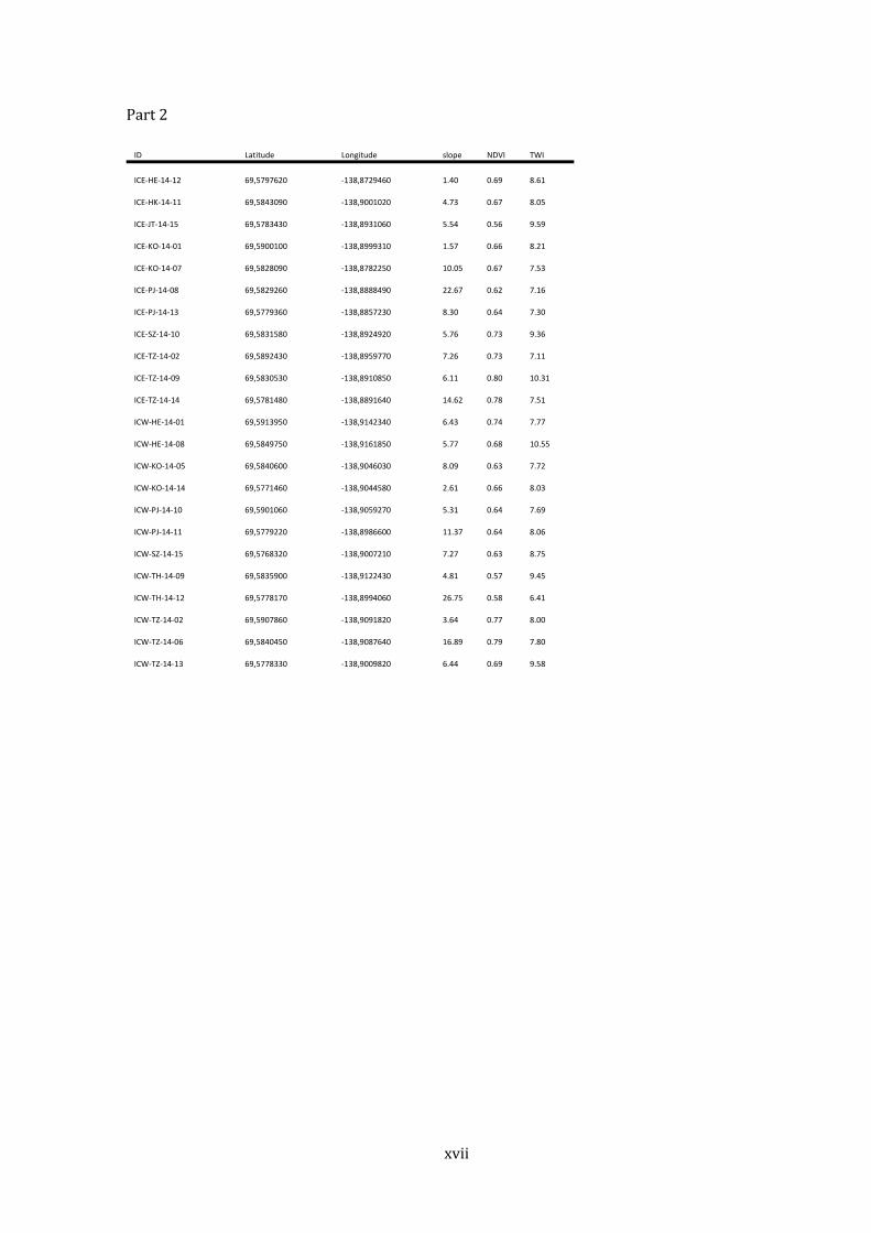
xvii

Part2

ID  Latitude  Longitude  slope  NDVI  TWI 

ICE‐HE‐14‐12  69,5797620  ‐138,8729460  1.40  0.69  8.61 

ICE‐HK‐14‐11  69,5843090  ‐138,9001020  4.73  0.67  8.05 

ICE‐JT‐14‐15  69,5783430  ‐138,8931060  5.54  0.56  9.59 

ICE‐KO‐14‐01  69,5900100  ‐138,8999310  1.57  0.66  8.21 

ICE‐KO‐14‐07  69,5828090  ‐138,8782250  10.05  0.67  7.53 

ICE‐PJ‐14‐08  69,5829260  ‐138,8888490  22.67  0.62  7.16 

ICE‐PJ‐14‐13  69,5779360  ‐138,8857230  8.30  0.64  7.30 

ICE‐SZ‐14‐10  69,5831580  ‐138,8924920  5.76  0.73  9.36 

ICE‐TZ‐14‐02  69,5892430  ‐138,8959770  7.26  0.73  7.11 

ICE‐TZ‐14‐09  69,5830530  ‐138,8910850  6.11  0.80  10.31 

ICE‐TZ‐14‐14  69,5781480  ‐138,8891640  14.62  0.78  7.51 

ICW‐HE‐14‐01  69,5913950  ‐138,9142340  6.43  0.74  7.77 

ICW‐HE‐14‐08  69,5849750  ‐138,9161850  5.77  0.68  10.55 

ICW‐KO‐14‐05  69,5840600  ‐138,9046030  8.09  0.63  7.72 

ICW‐KO‐14‐14  69,5771460  ‐138,9044580  2.61  0.66  8.03 

ICW‐PJ‐14‐10  69,5901060  ‐138,9059270  5.31  0.64  7.69 

ICW‐PJ‐14‐11  69,5779220  ‐138,8986600  11.37  0.64  8.06 

ICW‐SZ‐14‐15  69,5768320  ‐138,9007210  7.27  0.63  8.75 

ICW‐TH‐14‐09  69,5835900  ‐138,9122430  4.81  0.57  9.45 

ICW‐TH‐14‐12  69,5778170  ‐138,8994060  26.75  0.58  6.41 

ICW‐TZ‐14‐02  69,5907860  ‐138,9091820  3.64  0.77  8.00 

ICW‐TZ‐14‐06  69,5840450  ‐138,9087640  16.89  0.79  7.80 

ICW‐TZ‐14‐13  69,5778330  ‐138,9009820  6.44  0.69  9.58 

xviii

RScript

# Boxplots for TOC,TN and CN by Ecoclass and Vegclass par(mfrow = c(1,1)) boxplot(SOC_30cm ~ecoclass,data=icecreek_data, main="TOC (0-30cm)", cex.axis=1.5, cex.main=1.8, ylab="TOC (kg/m2)", cex.lab=1.5) boxplot(SOC_30cm ~vegname,data=icecreek_data, main="TOC (0-30cm)", cex.main=1.8, cex.axis=1.5) boxplot(SOC_active ~ecoclass,data=icecreek_data,main="TOC (Active Layer)", cex.main=1.8,cex.lab=1.5,cex.axis=1.5, ylab="TOC (kg/m2)", xlab="Ecological Class") boxplot(SOC_active ~vegname,data=icecreek_data, main="TOC (Active Layer)", cex.main=1.8, cex.lab=1.5,cex.axis=1.5,xlab="Vegetation Class") boxplot(TN_30cm ~ecoclass,data=icecreek_data, main="TN (0-30cm)", cex.main=1.8, cex.axis=1.5, cex.lab=1.5, ylab="TN (kg/m2)") boxplot(TN_30cm ~vegname,data=icecreek_data, main="TN (0-30cm)", cex.main=1.8, cex.axis=1.5) boxplot(TN_active ~ecoclass,data=icecreek_data, main="TN (Active Layer)", cex.main=1.8,cex.lab=1.5,cex.axis=1.5, ylab="TN (kg/m2)", xlab="Ecological Class") boxplot(TN_active ~vegname,data=icecreek_data, main="TN (Active Layer)", cex.main=1.8, cex.lab=1.5,cex.axis=1.5,xlab="Vegetation Class") boxplot(CN ~ecoclass,data=icecreek_data, main="CN ratio in topsoil", cex.main=1.8, cex.lab=1.5,cex.axis=1.5,ylab="CN ratio") boxplot(CN ~vegname,data=icecreek_data, main="CN ratio in topsoil", cex.main=1.8,cex.axis=1.5) boxplot(depth ~ecoclass,data=icecreek_data, main="Active Layer Depth", cex.main=1.8,cex.lab=1.5,cex.axis=1.5, xlab="Ecological Class", ylab="Active Layer Depth (cm)") boxplot(depth ~vegname,data=icecreek_data, main="Active Layer Depth", cex.main=1.8,cex.lab=1.5,cex.axis=1.5, xlab="Vegetation Class") boxplot(CN_30 ~ecoclass,data=icecreek_dataCN, main="CN Ratio (0-30cm)", cex.main=1.8, cex.lab=1.5,cex.axis=1.5) boxplot(CN_30 ~vegname,data=icecreek_dataCN, main="CN Ratio (0-30cm)", cex.main=1.8,cex.axis=1.5) boxplot(CN_active ~ecoclass,data=icecreek_dataCN, main="CN Ratio (Active Layer)", cex.main=1.8, cex.lab=1.5,cex.axis=1.5) boxplot(CN_active ~vegname,data=icecreek_dataCN, main="CN Ratio (Active Layer)", cex.main=1.8,cex.axis=1.5)

xix

# Boxplots for Transects par(mfrow = c(2,2)) boxplot(SOC_30cm ~streamsection,data=icecreek_data, main="TOC (0-30cm)", xlab="Stream Section", ylab="TOC (kg/m2)",cex.main=1.8, cex.lab=1.5,cex.axis=1.5) boxplot(TN_30cm ~streamsection,data=icecreek_data, main="TN (0-30cm)", xlab="Stream Section", ylab="TN (kg/m2)", cex.main=1.8, cex.lab=1.5,cex.axis=1.5) boxplot(CN ~streamsection,data=icecreek_dataCN, main="CN Ratio (0-30cm)", xlab="Stream Section", ylab="CN Ratio", cex.main=1.8, cex.lab=1.5,cex.axis=1.5) boxplot(CN_30 ~streamsection,data=icecreek_streamCN, main="CN Ratio Creek (0-30cm)", xlab="Stream Section", ylab="CN Ratio", cex.main=1.8, cex.lab=1.5,cex.axis=1.5) # Example Anova and Tukey post hoc test depth.aov <- aov(icecreek_data$depth~icecreek_data$vegname) summary(depth.aov) TukeyHSD(depth.aov) # Spearmann correlation matrix cor(spearmann, method= c("spearman")) rcorr(X, type=c("spearman")) X<-as.matrix(spearmann)

xx

#PCA ECO CLASS #Create category ecoclass <- ice_creek_select[, 3] #define columns soil<-ice_creek_select[, 6:21] #run PCA soil.pca <- prcomp(soil, center = TRUE, scale. = TRUE) #display PCA print(soil.pca) library(devtools) install_github("ggbiplot", "vqv") library(ggbiplot) g <- ggbiplot(soil.pca, obs.scale = 1, var.scale = 1, groups = ecoclass, ellipse = TRUE, circle = FALSE, varname.size = 6,colour = "black", varname.adjust = 1.5) g <- g + geom_point(aes( shape = groups, color = groups), size=5, ) + scale_shape_manual(values = 0:length(unique(ecoclass)))+ scale_colour_manual (values = c("blue","dark blue", " dark green","Yellow","brown", "red", "green")) g<- g + theme_bw() print(g)

xxi

# NMDS dat <- ice_creek_vegetation dat plot(dat) attach(dat) names(dat) library(permute) library(vegan) library(MASS) veg.pca<-rda(dat[,3:53]) veg.pca head(veg.pca) envdat<-dat[,1:2] envdat envi_pca<-envfit(veg.pca, envdat, permu=999, na.rm=TRUE) veg.pca <- dat[,1:53] plot(veg.pca) veg.dis<-vegdist(dat[,3:53]) veg.mds0<-monoMDS(veg.dis) stressplot(veg.mds0, veg.dis) ordiplot(veg.mds0, type="t") envdat<-dat[,1:2] envdat envi_mds<-envfit(veg.mds0, envdat, permu=999, na.rm=TRUE) envi_mds plot(envi_mds, p.max=0.2) veg.mds<-metaMDS(dat[,3:53]) veg.mds head(veg.mds) attach(dat) par(mfrow=c(1,1)) plot(veg.mds,display=c("species"), type="n", xlim=c(-2,2), ylim=c(-1.5,1.5)) points(veg.mds, display=c("sites"), choices=c(1,2), select=Type=="HE", col="green", pch=1) points(veg.mds, display=c("sites"), choices=c(1,2), select=Type=="HK", col="blue", pch=2) points(veg.mds, display=c("sites"), choices=c(1,2), select=Type=="KO", col="brown", pch=3) points(veg.mds, display=c("sites"), choices=c(1,2), select=Type=="TH", col="purple", pch=4) points(veg.mds, display=c("sites"), choices=c(1,2), select=Type=="PJ", col="darkblue", pch=5) points(veg.mds, display=c("sites"), choices=c(1,2), select=Type=="SZ", col="black", pch=6)

xxii

points(veg.mds, display=c("sites"), choices=c(1,2), select=Type=="TZ", col="pink", pch=7) points(veg.mds, display=c("sites"), choices=c(1,2), select=Type=="NN", col="red", pch=8) legend(x=1.5,y=1.8, cex= 0.8, c("Herschel", "He-Komakuk", "Komakuk","Thrasher", "Plover Jaeger", "Shrub Zone", "Transitional", "not known"), col=c("green","blue", "brown","purple", "darkblue","black","pink","red"), pch=c(1,2,3,4,5,6,7,8) ) #GGPLOT for NMDS data.scores <- as.data.frame(scores(veg.mds)) site<-ice_creek_vegetation$Point data.scores$site <- site Type <- ice_creek_vegetation$Type data.scores$Type <- Type head(data.scores) species.scores <- as.data.frame(scores(veg.mds, "species")) species.scores$species <- rownames(species.scores) head(species.scores) library(ggplot2) data.scores$Type <- factor(data.scores$Type) ggplot() + geom_point(data=data.scores,aes(x=NMDS1,y=NMDS2,shape=Type,colour=Type),size=4) + scale_shape_manual(values=1:nlevels(data.scores$Type))+ geom_vline(aes(xintercept=0))+ geom_hline(aes(yintercept=0))+ + # add the site labels scale_colour_manual(values=c("HE" = "blue", "HK" = "dark blue", "KO"= "dark green", "TH"="red", "PJ"="yellow", "SZ"="brown", "TZ"="green")) + coord_equal() + theme_bw()+ theme(axis.text.x = element_blank(), # remove x-axis text axis.text.y = element_blank(), # remove y-axis text axis.ticks = element_blank(), # remove axis ticks axis.title.x = element_text(size=18), # remove x-axis labels axis.title.y = element_text(size=18), # remove y-axis labels panel.background = element_blank(), panel.grid.major = element_blank(), #remove major-grid labels panel.grid.minor = element_blank(), #remove minor-grid labels plot.background = element_blank())

xxiii

Eidesstattliche Erklärung

HiermitversichereichanEidesstatt,dassichdieMasterarbeitselbständigverfasstundkeine

anderenalsdieangegebenenQuellenundHilfsmittelbenutztunddieausfremdenQuellen

direktoderindirektübernommenenGedankenalssolchekenntlichgemachthabe.DieArbeit

habeichbisherkeinemanderenPrüfungsamtingleicherodervergleichbarerFormvorgelegt.

Siewurdebisherauchnichtveröffentlicht.Icherkläremichdamiteinverstanden,dassdie

ArbeitmitHilfeeinesPlagiatserkennungsdienstesaufenthaltenePlagiateüberprüftwird.

Ort,Datum IsabellEischeid