university of huddersfield repositoryeprints.hud.ac.uk/28334/3/oe-24-8-8997.pdf(20), 24869–24893...

Phase and fringe order determination in wavelength scanning interferometry

Giuseppe Moschetti,1,2,* Alistair Forbes,1 Richard K Leach,3 Xiang Jiang,2 and Daniel O’Connor1

1National Physical Laboratory, Hampton Road, Teddington, Middlesex, TW11 0LW, UK 2Centre for Precision Technologies, University of Huddersfield, Huddersfield, West Yorkshire, HD1 3DH, UK

3Manufacturing Metrology Team, University of Nottingham, University Park, Nottingham NG72RD, UK *[email protected]

Abstract: A method to obtain unambiguous surface height measurements using wavelength scanning interferometry with an improved repeatability, comparable to that obtainable using phase shifting interferometry, is reported. Rather than determining the conventional fringe frequency-derived z height directly, the method uses the frequency to resolve the fringe order ambiguity, and combine this information with the more accurate and repeatable fringe phase derived z height. A theoretical model to evaluate the method’s performance in the presence of additive noise is derived and shown to be in good agreement with experiments. The measurement repeatability is improved by a factor of ten over that achieved when using frequency information alone, reaching the sub-nanometre range. Moreover, the z-axis non-linearity (bleed-through or ripple error) is reduced by a factor of ten. These order of magnitude improvements in measurement performance are demonstrated through a number of practical measurement examples. Published by The Optical Society under the terms of the Creative Commons Attribution 4.0 License. Further distribution of this work must maintain attribution to the author(s) and the published article’s title, journal citation, and DOI. OCIS codes: (120.0120) Instrumentation, measurement, and metrology; (120.3180) Interferometry; (120.6650) Surface measurements, figure; (120.4640) Optical instruments; (120.2650) Fringe analysis.

References and links 1. P. de Groot, “Principles of interference microscopy for the measurement of surface topography,” Adv. Opt.

Photonics 7(1), 1–65 (2015). 2. J. A. N. Buytaert and J. J. J. Dirckx, “Study of the performance of 84 phase-shifting algorithms for

interferometry,” J. Opt. 40(3), 114–131 (2011). 3. M. Servin, J. C. Estrada, and J. A. Quiroga, “The general theory of phase shifting algorithms,” Opt. Express

17(24), 21867–21881 (2009). 4. A. Harasaki, J. Schmit, and J. C. Wyant, “Improved vertical-scanning interferometry,” Appl. Opt. 39(13), 2107–

2115 (2000). 5. P. de Groot and L. Deck, “Surface Profiling by Analysis of White-light Interferograms in the Spatial Frequency

Domain,” J. Mod. Opt. 42(2), 389–401 (1995). 6. K. G. Larkin, “Efficient nonlinear algorithm for envelope detection in white light interferometry,” J. Opt. Soc.

Am. A 13(4), 832–843 (1996). 7. G. Barwood, P. Gill, and W. Rowley, “Laser diodes for length determination using swept-frequency

interferometry,” Meas. Sci. Technol. 4(9), 988–994 (1993). 8. J. A. Stone, A. Stejskal, and L. Howard, “Absolute interferometry with a 670-nm external cavity diode laser,”

Appl. Opt. 38(28), 5981–5994 (1999). 9. X. Jiang, K. Wang, F. Gao, and H. Muhamedsalih, “Fast surface measurement using wavelength scanning

interferometry with compensation of environmental noise,” Appl. Opt. 49(15), 2903–2909 (2010). 10. F. Gao, H. Muhamedsalih, and X. Jiang, “Surface and thickness measurement of a transparent film using

wavelength scanning interferometry,” Opt. Express 20(19), 21450–21456 (2012). 11. A. Davila, J. M. Huntley, C. Pallikarakis, P. D. Ruiz, and J. M. Coupland, “Wavelength scanning interferometry

using a Ti:Sapphire laser with wide tuning range,” Opt. Lasers Eng. 50(8), 1089–1096 (2012). 12. V. Badami and P. De Groot, Displacement Measuring Interferometry (Taylor & Francis, 2013).

#258089 Received 22 Jan 2016; revised 10 Mar 2016; accepted 8 Apr 2016; published 15 Apr 2016 © 2016 OSA 18 Apr 2016 | Vol. 24, No. 8 | DOI:10.1364/OE.24.008997 | OPTICS EXPRESS 8997

http://creativecommons.org/licenses/by/4.0/

http://creativecommons.org/licenses/by/4.0/

13. D. Malacara, Optical Shop Testing, Third ed., Wiley Series in Pure and Applied Optics (Wiley, 2007). 14. J. Dale, B. Hughes, A. J. Lancaster, A. J. Lewis, A. J. H. Reichold, and M. S. Warden, “Multi-channel absolute

distance measurement system with sub ppm-accuracy and 20 m range using frequency scanning interferometry and gas absorption cells,” Opt. Express 22(20), 24869–24893 (2014).

15. L. L. Deck, “Absolute distance measurements using FTPSI with a widely tunable IR laser,” Proc. SPIE 4778, 218–226 (2002).

16. X. Dai and K. Seta, “High-accuracy absolute distance measurement by means of wavelength scanning heterodyne interferometry,” Meas. Sc. Technol. 9(7), 1031 (1998).

17. P. D. Ruiz, Y. Zhou, J. M. Huntley, and R. D. Wildman, “Depth-resolved whole-field displacement measurement using wavelength scanning interferometry,” J. Opt. A, Pure Appl. Opt. 6(7), 679–683 (2004).

18. Y.-S. Ghim, A. Suratkar, and A. Davies, “Reflectometry-based wavelength scanning interferometry for thickness measurements of very thin wafers,” Opt. Express 18(7), 6522–6529 (2010).

19. P. de Groot, “Measurement of transparent plates with wavelength-tuned phase-shifting interferometry,” Appl. Opt. 39(16), 2658–2663 (2000).

20. G. Moschetti, H. Muhamedsalih, D. O’Connor, X. Jiang, and R. K. Leach, “Vertical axis non-linearities in wavelength scanning interferometry,” in 11th International Conference and Exhibition on Laser Metrology,Machine Tool, CMM & Robotic Performance (2015), pp. 31–39.

21. P. de Groot, X. Colonna de Lega, J. Kramer, and M. Turzhitsky, “Determination of Fringe Order in White-Light Interference Microscopy,” Appl. Opt. 41(22), 4571–4578 (2002).

22. J. C. Estrada, M. Servin, and J. A. Quiroga, “A self-tuning phase-shifting algorithm for interferometry,” Opt. Express 18(3), 2632–2638 (2010).

23. L. Deck and P. de Groot, “High-speed noncontact profiler based on scanning white-light interferometry,” Appl. Opt. 33(31), 7334–7338 (1994).

24. C. Ai and E. L. Novak, “Centroid approach for estimating modulation peak in broad-bandwidth interferometry,” U.S. patent 5,633,715 (1997).

25. Y.-S. Ghim and A. Davies, “Complete fringe order determination in scanning white-light interferometry using a Fourier-based technique,” Appl. Opt. 51(12), 1922–1928 (2012).

26. P. de Groot and L. Deck, “Surface Profiling by Analysis of White-light Interferograms in the Spatial Frequency Domain,” J. Mod. Opt. 42(2), 389–401 (1995).

27. H. Muhamedsalih, F. Gao, and X. Jiang, “Comparison study of algorithms and accuracy in the wavelength scanning interferometry,” Appl. Opt. 51(36), 8854–8862 (2012).

28. J. Kato and I. Yamaguchi, “Height gauging by wavelength-scanning interferometry with phase detection,” SPIE Conf. Opt. Eng. Sens. Technol. 3740, (1999).

29. J. Kato and I. Yamaguchi, “Phase-Shifting Fringe Analysis for Laser Diode Wavelength-Scanning Interferometer,” Opt. Rev. 7(2), 158–163 (2000).

30. I. Yamaguchi, A. Yamamoto, and M. Yano, “Surface topography by wavelength scanning interferometry,” Opt. Eng. 39(1), 40 (2000).

31. M. Takeda, H. Ina, and S. Kobayashi, “Fourier-transform method of fringe-pattern analysis for computer-based topography and interferometry,” J. Opt. Soc. Am. 72(1), 156 (1982).

32. Y.-S. Ghim, A. Suratkar, A. Davies, and Y.-W. Lee, “Absolute thickness measurement of silicon wafer using wavelength scanning interferometer,” Proc. SPIE 8133, 813312 (2011).

33. F. Pavese and A. B. Forbes, Data Modeling for Metrology and Testing in Measurement Science, Modeling and Simulation in Science, Engineering and Technology (Birkhäuser Basel, 2008).

34. D. C. Rife and R. R. Boorstyn, “Single-Tone Parameter Estimation from Discrete-Time Observations,” IEEE Trans. Inf. Theory 20(5), 591–598 (1974).

35. H. L. Van Trees and K. L. Bell, Detection Estimation and Modulation Theory, Part I, 2nd ed. (John Wiley & Sons, 2013).

36. E. Peterson, “A Not-so-Characteristic Equation: the Art of Linear Algebra,” 1–15 (2007). Available at http://arxiv.org/abs/0712.2058.

37. C. L. Giusca, R. K. Leach, F. Helary, T. Gutauskas, and L. Nimishakavi, “Calibration of the scales of areal surface topography-measuring instruments: part 1. Measurement noise and residual flatness,” Meas. Sci. Technol. 23(3), 035008 (2012).

38. A. J. Jerri, “The Shannon Sampling Theorem-Its Various Extensions and Applications: A Tutorial Review,” Proc. IEEE 65(11), 1565–1596 (1977).

39. P. De Groot, J. Beverage, Z. Corporation, and L. B. Road, “Calibration of the amplification coefficient in interference microscopy by means of a wavelength standard,” in SPIE Optical Metrology (2015).

40. R. Mandal, J. Coupland, R. Leach, and D. Mansfield, “Coherence scanning interferometry: measurement and correction of three-dimensional transfer and point-spread characteristics,” Appl. Opt. 53(8), 1554–1563 (2014).

41. P. J. De Groot, “Progress in the specification of optical instruments for the measurement of surface form and texture,” Proc. SPIE 9110, Dimens. Opt. Metrol. Insp. Pract. Appl. III 9110, 1–12 (2014).

42. R. K. Leach, “Is one step height enough,” in Proceedings of ASPE (2015).


1. Introduction

Interferometry is a widely-used technique to measure displacement and, when combined with an optical microscope, can allow the measurement of areal surface topography. The most common areal interferometry techniques for surface topography measurement are phase shifting interferometry (PSI) and coherence scanning interferometry (CSI), and many algorithms to estimate the surface heights from the interference fringes exist for these techniques [1–6].

Wavelength scanning interferometry (WSI) is a competing technique due to its potential for very short measurement times since its operation does not require a mechanical scan, at the expense of a measurement range limited by the objective lens depth of focus [7–11]. The most common method of surface extraction used by state-of-the-art WSI instruments utilises only the phase change information obtained from the fringe data [12–14]. Improvement in the measurement performance of the WSI technique has been previously reported by combining the phase change (i.e. the frequency) and the absolute phase of the fringe pattern to measure plate thicknesses and refractive index [15] and for point-like displacement measurement with a heterodyne interferometer [16]. Other techniques exist for measuring surfaces or film thicknesses with WSI instruments, which also exploit the absolute phase information that is available. These methods include phase estimation through Fourier transform (FT) [17], model-based techniques [18] or PSI algorithms to suppress spurious reflections [19]. However, the FT and model-based techniques require the assumption that the surface is continuous to unwrap the ambiguous phase, therefore, limiting their application. Furthermore, the FT method is subject to errors due to spectral leakage [20], and the model-based techniques are computationally intensive. PSI algorithms must be designed for specific frequencies, requiring foreknowledge of the interference pattern frequency.

In this paper, we describe how the demodulated phase can be employed to obtain absolute areal surface topography measurements using WSI, with repeatability comparable to PSI and CSI, without the assumption of surface continuity or previous knowledge of the interference pattern frequency. A similar development was a key step in improving the performance of CSI instruments [4,21]. Additionally, we describe an analytical model to quantify the improvements when estimating the surface via phase change or absolute phase in presence of additive noise. The method, hereby described, permits the development of adaptive linear filtering algorithms that can be tuned for the specific needs of WSI [3,22], resulting in an accurate and computationally fast algorithm for WSI instruments.

This paper is structured as follows: section 2 introduces the interferometric technique with a particular focus on WSI and the optical configuration, section 3 describes in detail how to combine phase and frequency to resolve the fringe order and improve the estimation of the surface height for WSI. Section 4 describes the model to calculate the Cramer-Rao bound (CRB) for the estimation of height for the standard method and the improved method proposed here. Section 5 reports on a variety of measurements to demonstrate the improvements and section 6 is a conclusion.

2. Interferometer technique

The intensity of an interference signal can be written as:

( , ) ( )[1 ( ) cos(2 )]m mI k z q k V k kzπ= + (1)

where k is the wavenumber of the interfering light, zm is the optical path difference (OPD) between the measurement and reference arm of the interferometer, q(k) is the signal background and V(k) is the fringe visibility. In PSI and CSI, the phase is modulated by changing zm, i.e. by moving the sample or the reference mirror whilst the illumination (k) is kept constant. In WSI, the phase is instead modulated by changing the wavelength, i.e. by


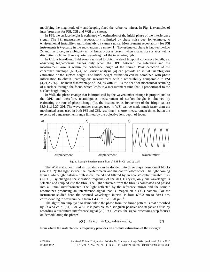
modifying the magnitude of and keeping fixed the reference mirror. In Fig. 1, examples of interferograms for PSI, CSI and WSI are shown.

In PSI, the surface height is estimated via estimation of the initial phase of the interference signal. The PSI measurement repeatability is limited by phase noise due, for example, to environmental instability, and ultimately by camera noise. Measurement repeatability for PSI instruments is typically in the sub-nanometre range [1]. The estimated phase is known modulo 2π and, therefore, an ambiguity in the fringe order is present when measuring surfaces with a discontinuity larger than a quarter wavelength of the interfering light.

In CSI, a broadband light source is used to obtain a short temporal coherence length, i.e. observing high-contrast fringes only when the OPD between the reference and the measurement arm is within the coherence length of the source. Peak detection of the coherence envelope [6,23,24] or Fourier analysis [4] can provide an initial unambiguous estimation of the surface height. The initial height estimation can be combined with phase information to obtain unambiguous measurement with a repeatability comparable to PSI [4,21,25,26]. The main disadvantage of CSI, as with PSI, is the need for mechanical scanning of a surface through the focus, which leads to a measurement time that is proportional to the surface height range.

In WSI, the phase change that is introduced by the wavenumber change is proportional to the OPD and, therefore, unambiguous measurement of surface height is obtained by estimating the rate of phase change (i.e. the instantaneous frequency) of the fringe pattern [8,9,11,12,27–30]. The wavenumber changes used in WSI can be made much faster than the mechanical scans used in both PSI and CSI, resulting in shorter measurement times, but at the expense of a measurement range limited by the objective lens depth of focus.

Fig. 1. Example interferograms from a) PSI, b) CSI and c) WSI.

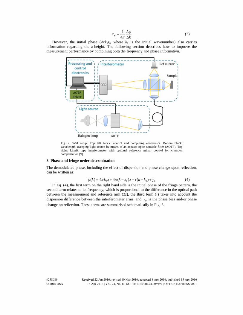
The WSI instrument used in this study can be divided into three major component blocks (see Fig. 2): the light source, the interferometer and the control electronics. The light coming from a white-light halogen bulb is collimated and filtered by an acousto-optic tuneable filter (AOTF). By changing the vibration frequency of the AOTF crystal, only one wavelength is selected and coupled into the fibre. The light delivered from the fibre is collimated and passed into a Linnik interferometer. The light reflected by the reference mirror and the sample recombines producing an interference signal that is imaged on a CCD camera. For the instrument studied here, the scanned wavelength interval is from 695.2 nm to 589.1 nm, corresponding to wavenumbers from 1.43 µm−1 to 1.70 µm−1.

The algorithm employed to demodulate the phase from the fringe pattern is that described by Takeda et. al [31]. For WSI, it is possible to distinguish positive and negative OPDs by recording a quadrature interference signal [29]. In all cases, the signal processing step focuses on demodulating the phase:

0 0( ) 4 4 4 ( )m m mk kz k z k k zϕ π π π= = + − (2)

from which the instantaneous frequency provides an absolute estimation of the z-height:


14mz

kϕ

π∆

=∆

(3)

However, the initial phase (4πk0zm where k0 is the initial wavenumber) also carries information regarding the z-height. The following section describes how to improve the measurement performance by combining both the frequency and phase information.

Fig. 2. WSI setup. Top left block: control and computing electronics. Bottom block: wavelength sweeping light source by means of an acousto-optic tuneable filter (AOTF). Top right: Linnik type interferometer with optional reference mirror control for vibration compensation [9].

3. Phase and fringe order determination

The demodulated phase, including the effect of dispersion and phase change upon reflection, can be written as:

0 0 0 0( ) 4 4 ( ) ( )k k z k k z k kϕ π π τ γ= + − + − + (4) In Eq. (4), the first term on the right hand side is the initial phase of the fringe pattern, the

second term relates to its frequency, which is proportional to the difference in the optical path between the measurement and reference arm (2z), the third term (τ) takes into account the dispersion difference between the interferometer arms, and 0γ is the phase bias and/or phase change on reflection. These terms are summarised schematically in Fig. 3.


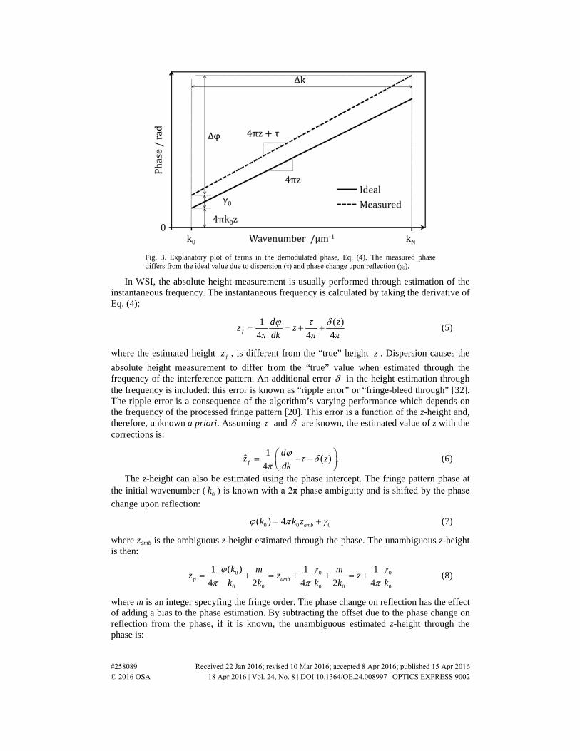
Fig. 3. Explanatory plot of terms in the demodulated phase, Eq. (4). The measured phase differs from the ideal value due to dispersion (τ) and phase change upon reflection (γ0).

In WSI, the absolute height measurement is usually performed through estimation of the instantaneous frequency. The instantaneous frequency is calculated by taking the derivative of Eq. (4):

1 ( )4 4 4f

d zz zdkϕ τ d

π π π= = + + (5)

where the estimated height fz , is different from the “true” height z . Dispersion causes the absolute height measurement to differ from the “true” value when estimated through the frequency of the interference pattern. An additional error d in the height estimation through the frequency is included: this error is known as “ripple error” or “fringe-bleed through” [32]. The ripple error is a consequence of the algorithm’s varying performance which depends on the frequency of the processed fringe pattern [20]. This error is a function of the z-height and, therefore, unknown a priori. Assuming τ and d are known, the estimated value of z with the corrections is:

1ˆ ( ) .4f

dz zdkϕ τ d

π = − −

(6)

The z-height can also be estimated using the phase intercept. The fringe pattern phase at the initial wavenumber ( 0k ) is known with a 2π phase ambiguity and is shifted by the phase change upon reflection:

0 0 0( ) 4 ambk k zϕ π γ= + (7)

where zamb is the ambiguous z-height estimated through the phase. The unambiguous z-height is then:

0 0 0

0 0 0 0 0

( )1 1 14 2 4 2 4p amb

k m mz z zk k k k k

ϕ γ γπ π π

= + = + + = + (8)

where m is an integer specyfing the fringe order. The phase change on reflection has the effect of adding a bias to the phase estimation. By subtracting the offset due to the phase change on reflection from the phase, if it is known, the unambiguous estimated z-height through the phase is:


( )0 00

1ˆ ( ) 24

z k mk

ϕ π γπ

= + − (9)

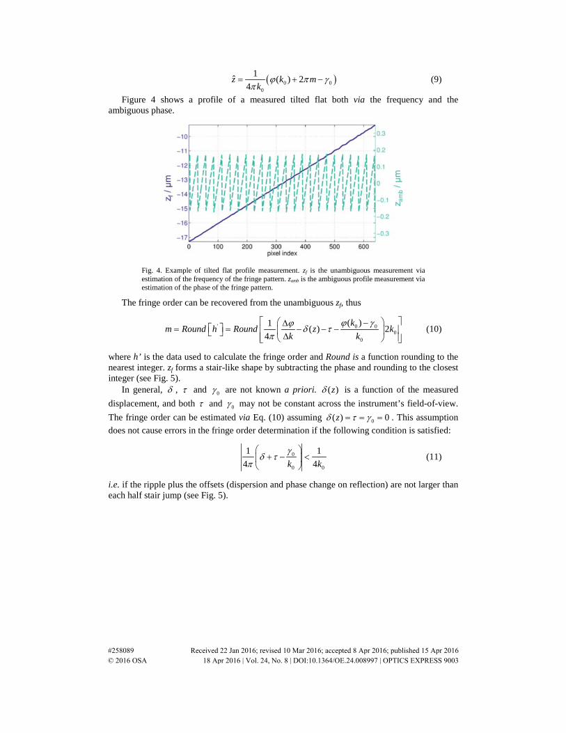
Figure 4 shows a profile of a measured tilted flat both via the frequency and the ambiguous phase.

Fig. 4. Example of tilted flat profile measurement. zf is the unambiguous measurement via estimation of the frequency of the fringe pattern. zamb is the ambiguous profile measurement via estimation of the phase of the fringe pattern.

The fringe order can be recovered from the unambiguous zf, thus

' 0 00

0

( )1 ( ) 24

km Round h Round z k

k kϕ γϕ d τ

π −∆ = = − − − ∆

(10)

where h’ is the data used to calculate the fringe order and Round is a function rounding to the nearest integer. zf forms a stair-like shape by subtracting the phase and rounding to the closest integer (see Fig. 5).

In general, d , τ and 0γ are not known a priori. ( )zd is a function of the measured displacement, and both τ and 0γ may not be constant across the instrument’s field-of-view. The fringe order can be estimated via Eq. (10) assuming 0( ) 0zd τ γ= = = . This assumption does not cause errors in the fringe order determination if the following condition is satisfied:

0

0 0

1 14 4k k

γd τ

π

+ − <

(11)

i.e. if the ripple plus the offsets (dispersion and phase change on reflection) are not larger than each half stair jump (see Fig. 5).


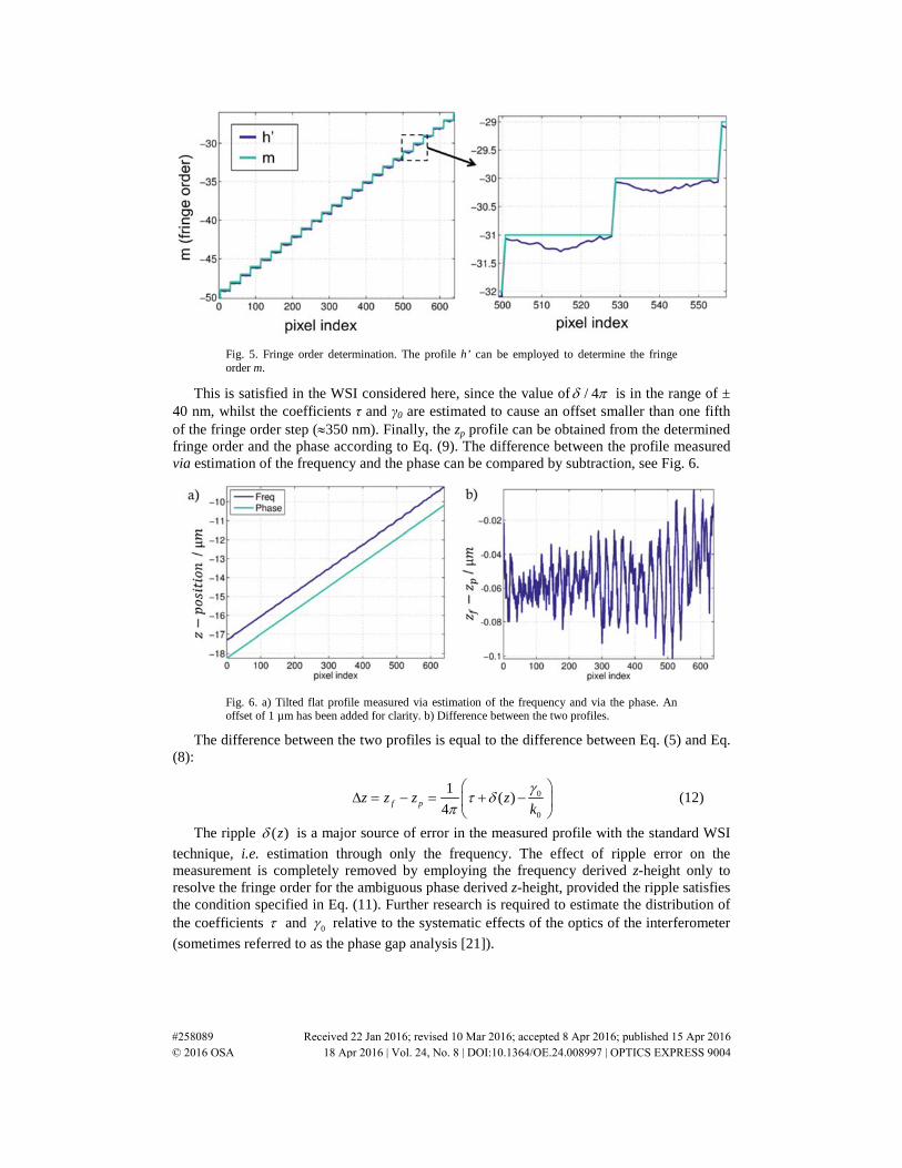
Fig. 5. Fringe order determination. The profile h’ can be employed to determine the fringe order m.

This is satisfied in the WSI considered here, since the value of / 4d π is in the range of ± 40 nm, whilst the coefficients τ and γ0 are estimated to cause an offset smaller than one fifth of the fringe order step (≈350 nm). Finally, the zp profile can be obtained from the determined fringe order and the phase according to Eq. (9). The difference between the profile measured via estimation of the frequency and the phase can be compared by subtraction, see Fig. 6.

Fig. 6. a) Tilted flat profile measured via estimation of the frequency and via the phase. An offset of 1 µm has been added for clarity. b) Difference between the two profiles.

The difference between the two profiles is equal to the difference between Eq. (5) and Eq. (8):

0

0

1 ( )4f pz z z z

kγ

τ dπ

∆ = − = + −

(12)

The ripple ( )zd is a major source of error in the measured profile with the standard WSI technique, i.e. estimation through only the frequency. The effect of ripple error on the measurement is completely removed by employing the frequency derived z-height only to resolve the fringe order for the ambiguous phase derived z-height, provided the ripple satisfies the condition specified in Eq. (11). Further research is required to estimate the distribution of the coefficients τ and 0γ relative to the systematic effects of the optics of the interferometer (sometimes referred to as the phase gap analysis [21]).


4. Cramer Rao Bound for frequency and phase estimation

A model has been developed to compare the performances of the z-height estimation through the frequency or the phase in the presence of additive noise. In the measurement, the surface z-height should be estimated from N observations (samples) of the interference pattern. The observational model perturbed by an additive random effect is given by:

( ) ( ) , [0,..., 1]n n nI S W n N= + ∈ −α α (13)

where In(α) is the nth observation point, i.e. the intensity recorded at the nth wavenumber kn, Sn(α) is the modelled ideal system response where α is the vector of unknown parameters and Wn is a random effect. For a given set of wavenumbers 1

0{ }Nn nk −

= , Sn(α) describes an N-

dimensional model surface in p, where p is the number of parameters in the vector α and N is the number of observed points. The observed data vector In(α) is the perturbed system response from the ideal response Sn(α), where α describes the true state of the system (see Fig. 7).

Fig. 7. System model response and its linear approximation. The ideal fringe pattern intensities observed at N points are a function of the model parameters α to the vector of observed data S(α) . Noise causes the observations to not be exactly at the ideal point along the system response curve, but in a point cloud around the ideal. The statistical property of the noise can be propagated to obtain the uncertainty of the model parameters.

In vectorial form, Eq. (13) can be written as:

( )I S W= +α (14) The noise vector W is assumed zero-mean, white additive Gaussian noise and therefore its

uncertainty matrix (also called covariance or dispersion matrix) is equal to 2[ ]WU COV W σ= = ℑ , where ℑ is the identity matrix. The uncertainty matrix is a matrix

whose elements in the i,j position is the covariance between the i-th and the j-th elements of a vector of random variables. If the system response is linear, then ( )S α is a linear function of the parameter α , and the maximum-likelihood estimation method is of least-squares form [33]. Furthermore, if the estimation is unbiased, it is possible to propagate the effect of W to obtain the uncertainty matrix LSU associated with the least-squares estimate LSα . If the


system response ( )S α is not linear, the estimator is not biased and the noise is sufficiently small, the problem can still be linearized around the solution NLα to determine an approximate uncertainty matrix NLU [33]:

2 1[ ]TNLU J Jσ −≈ (15)

where J is the Jacobian matrix of the system response at the solution NLα defined as:

( )[0,..., 1]; [0,..., 1]

NL

nnj

j

SJ n N j p

α αα

=

∂= ∈ − ∈ −

∂α

(16)

The result of Eq. (15) and Eq. (16) is also known as the Cramer-Rao bound (CRB) and is a known result in the signal processing field both for real and complex tone estimation [34]. The CRB establishes a lower bound on the variance of the estimation of a deterministic parameter from measured data with additive noise [35]. For clarity, the CRB is adapted for the case in which the frequency, the amplitude and the phase are the unknown, and the z-height is the aim of the estimation.

For the case in which a complex fringe pattern is recorded, the system model is:

0 0[4 4 ( ) ]([ , , ]) [0,..., 1]p n fi k z k k zn f pS b z z be n Nπ π+ −= ∈ − (17)

where the parameter model vector [ , , ]f pb z z=α , i.e. the model unknowns are the amplitude, and two z-heights proportional to the frequency and phase. The propagated variance in the parameters estimation due to a perturbation in the observed data is:

1

2

0 000

b

NL f fp

fp p

cU c c

c cσ

− ≈

(18)

where

bc N= (19)

21

2 2 20

0(4 ) ( ) (4 ) ( 1)(2 1)

6

N

f nn

kc b k k b N N N dπ π−

=

= − = − −∑ (20)

20(4 )pc k b Nπ= (21)

1

2 20 0 0

0(4 ) ( ) (4 ) ( 1)

2

N

fp nn

kc b k k k b k N N dπ π−

=

= − = −∑ (22)

where the substitution 0nk k n kd− = and the formulae for the sum of the first (N – 1) integers

and the sum of their squares have been used (1 1

2

0 0

( 1) ( 1)(2 1);2 6

N N

n n

N N N N Nn n− −

= =

− − −= =∑ ∑ ).

The inverse of a symmetric matrix has an analytical solution:

2 1 2 [ ][ ][ ]

TT

NL T

adj J JU J Jdet J J

σ σ−≈ = (23)

where adj is the adjugate matrix of its argument and det the matrix determinant [36]. The adjugate matrix is the transpose of the cofactor matrix and, therefore:


22

2 12

2 2

0 0[ ] 0

( )0

0 000

p f fpT

NL b p b fpb p f fp

b fp b f

b

f fp

fp p

c c cU J J c c c c

c c c cc c c c

dd d Dd d

σσ

σ σ

−

− ≈ = − − −

= =

(24)

The elements along the diagonal of the matrix UNL are the propagated variance in the estimation of the parameters in the system model vectorα , i.e. the minimum achievable estimation variance in the presence of additive noise for the amplitude, the z-height estimated via the frequency and via the phase of the fringe pattern. Expanding the different contributions leads to:

222 2 2 2

0 0

42 2 2

0

(4 ) ( 1)(2 1) (4 ) (4 ) ( 1)6 2

(4 ) ( 1)( 1) .12

f p fpk kc c c b N N N k b N b k N N

b N N N k k

d dπ π π

π d

− = − − − −

= − +

(25)

and, therefore:

1 1b

b

dc N

= = (26)

2 2 2 2 3 2

2 2

1 12 1 12(4 ) ( 1)( 1) (4 )

1 12(4 )

pf

f p fp

cd

c c c b N N N k b N k

b N k

π d π d

π

= = ≈− − +

=∆

(27)

2 2 2 2 20 0

1 2(2 1) 1 4(4 ) ( 1) (4 )

fp

f p fp

c Ndc c c b N N k b Nkπ π

−= = ≈

− + (28)

2 2 2 20 0

6 1 6(4 ) ( 1) (4 )

fpfp

f p fp

cd

c c c b N N k k b N k kπ d π d− − −

= = ≈− +

(29)

where the substitution N k kd = ∆ has been used, and the approximations are valid for large N. df and dp are the variance in the estimation of the z-height via the frequency or the phase. The variance is always proportional to the inverse of the signal to noise ratio ( 2 2

1010 log [ / ]SNR b σ= ). The z-height estimation variance via the frequency is inversely proportional to the square of the wavenumber range ( N k kd = ∆ ), i.e. increasing the wavenumber range decreases the variance of the frequency estimation. Additionally, the phase and frequency variance is inversely proportional to the number of samples. The estimation via the phase is inversely proportional to the square of the wavenumber for which the phase is evaluated ( 0k ). In a wavelength period, the phase varies by 2π and, therefore, shorter wavelengths (larger wavenumbers) reduce the variance in the z-height estimation through the phase, as expected. For performance evaluation it is more convenient to use the root mean square error (RMSE) of the z-height estimation, being equal to the square root of the variance. For example, for a SNR of 20 dB ( / 10b σ = ) and 128 samples, the z-estimation RMSE through the frequency for a wavenumber range of 1.66 µm−1 to 1.43 µm−1 (wavelength


range from 600 nm to 700 nm) is approximately 10 nm. On the other hand, the z-estimation RMSE through the phase for a wavenumber of 1.43 µm−1 and, with the same parameters as the frequency estimation, is approximately 1 nm. The ratio between the RMSE through the frequency and the phase, for large N, is equal to:

20 0

2

12 34

f

p

d Nk kd kN k

= =∆∆

(30)

which, for the wavenumber values reported above corresponds to an improvement of the RMSE of the z-height estimation of approximately ten.

For the case where N is equal to 2, the model agrees with the improvement discussed by de Groot [1] for Fourier analysis of CSI interferograms and it is equal to:

02f

p

d kd k

=∆

(31)

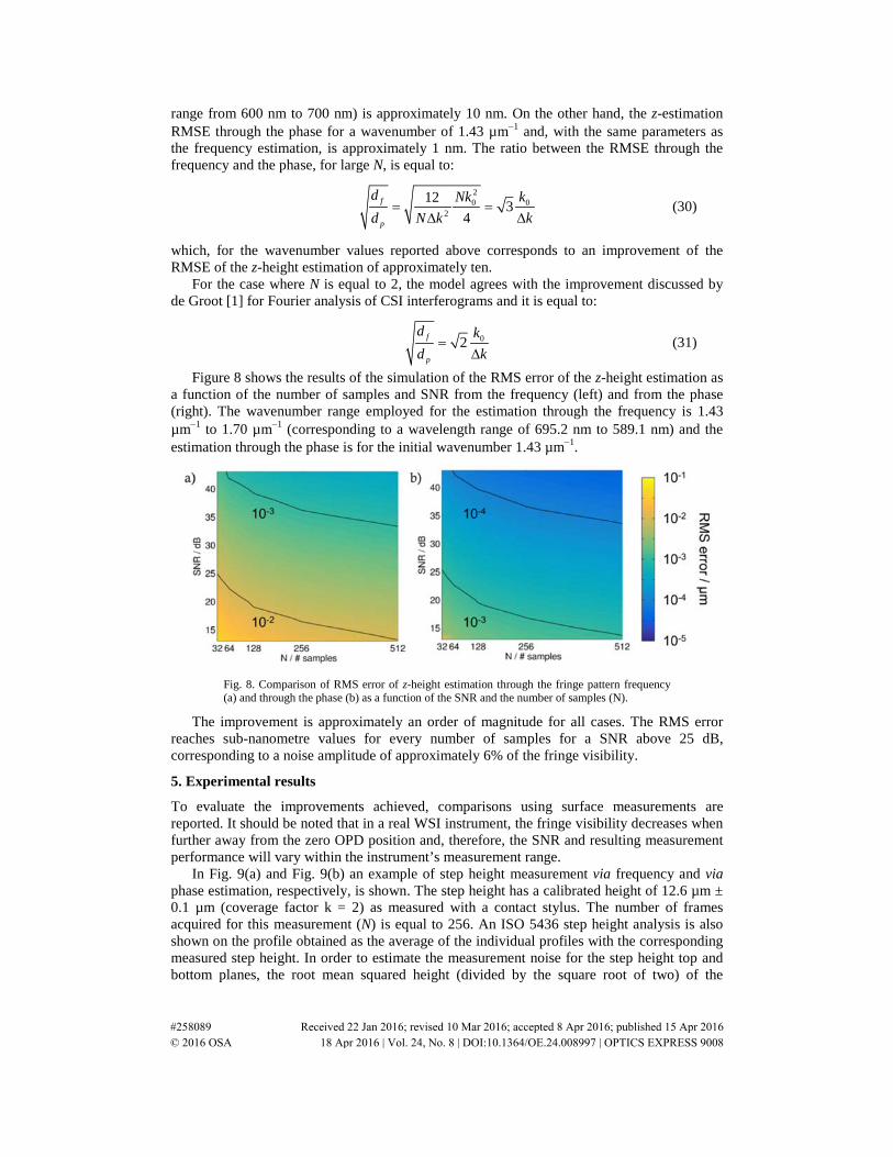
Figure 8 shows the results of the simulation of the RMS error of the z-height estimation as a function of the number of samples and SNR from the frequency (left) and from the phase (right). The wavenumber range employed for the estimation through the frequency is 1.43 µm−1 to 1.70 µm−1 (corresponding to a wavelength range of 695.2 nm to 589.1 nm) and the estimation through the phase is for the initial wavenumber 1.43 µm−1.

Fig. 8. Comparison of RMS error of z-height estimation through the fringe pattern frequency (a) and through the phase (b) as a function of the SNR and the number of samples (N).

The improvement is approximately an order of magnitude for all cases. The RMS error reaches sub-nanometre values for every number of samples for a SNR above 25 dB, corresponding to a noise amplitude of approximately 6% of the fringe visibility.

5. Experimental results

To evaluate the improvements achieved, comparisons using surface measurements are reported. It should be noted that in a real WSI instrument, the fringe visibility decreases when further away from the zero OPD position and, therefore, the SNR and resulting measurement performance will vary within the instrument’s measurement range.

In Fig. 9(a) and Fig. 9(b) an example of step height measurement via frequency and via phase estimation, respectively, is shown. The step height has a calibrated height of 12.6 µm ± 0.1 µm (coverage factor k = 2) as measured with a contact stylus. The number of frames acquired for this measurement (N) is equal to 256. An ISO 5436 step height analysis is also shown on the profile obtained as the average of the individual profiles with the corresponding measured step height. In order to estimate the measurement noise for the step height top and bottom planes, the root mean squared height (divided by the square root of two) of the


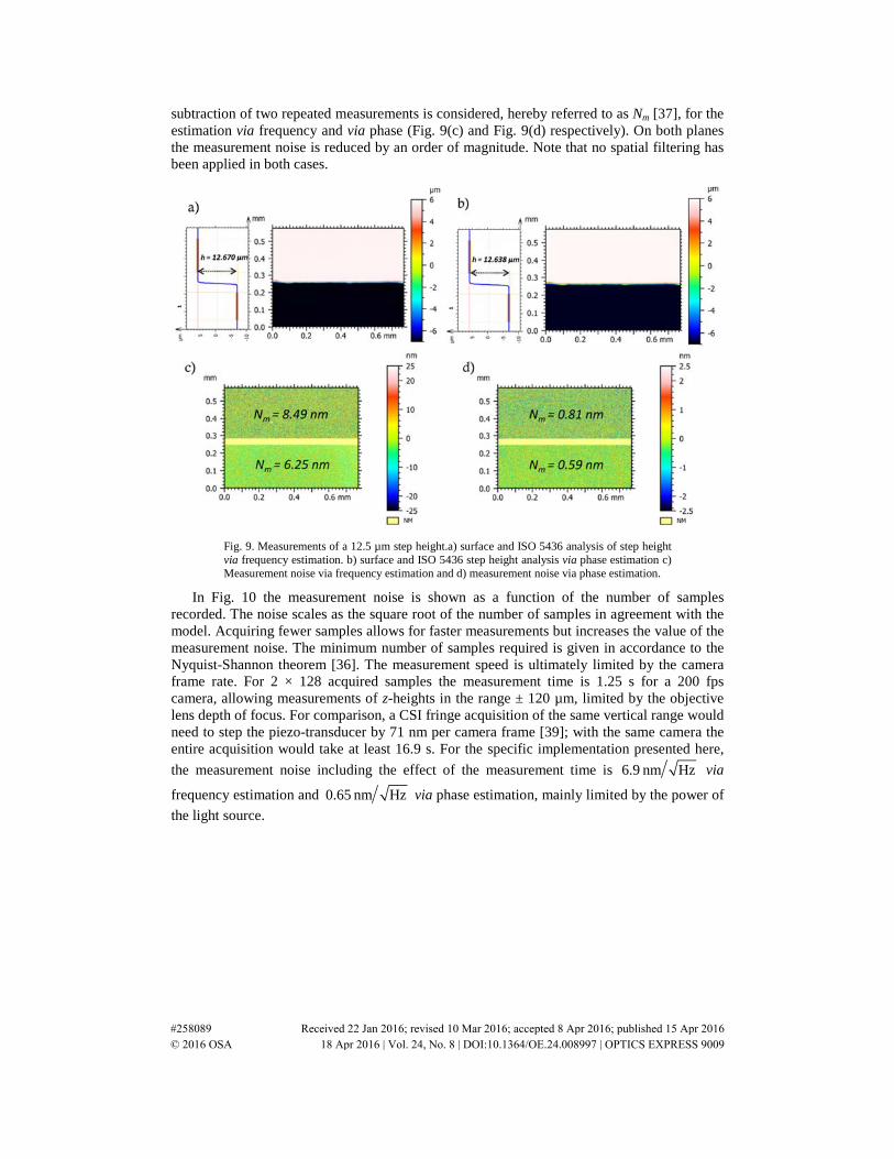
subtraction of two repeated measurements is considered, hereby referred to as Nm [37], for the estimation via frequency and via phase (Fig. 9(c) and Fig. 9(d) respectively). On both planes the measurement noise is reduced by an order of magnitude. Note that no spatial filtering has been applied in both cases.

Fig. 9. Measurements of a 12.5 µm step height.a) surface and ISO 5436 analysis of step height via frequency estimation. b) surface and ISO 5436 step height analysis via phase estimation c) Measurement noise via frequency estimation and d) measurement noise via phase estimation.

In Fig. 10 the measurement noise is shown as a function of the number of samples recorded. The noise scales as the square root of the number of samples in agreement with the model. Acquiring fewer samples allows for faster measurements but increases the value of the measurement noise. The minimum number of samples required is given in accordance to the Nyquist-Shannon theorem [36]. The measurement speed is ultimately limited by the camera frame rate. For 2 × 128 acquired samples the measurement time is 1.25 s for a 200 fps camera, allowing measurements of z-heights in the range ± 120 µm, limited by the objective lens depth of focus. For comparison, a CSI fringe acquisition of the same vertical range would need to step the piezo-transducer by 71 nm per camera frame [39]; with the same camera the entire acquisition would take at least 16.9 s. For the specific implementation presented here, the measurement noise including the effect of the measurement time is 6.9 nm Hz via

frequency estimation and 0.65 nm Hz via phase estimation, mainly limited by the power of the light source.


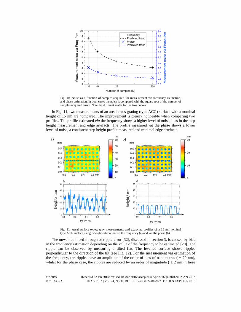
Fig. 10. Noise as a function of samples acquired for measurement via frequency estimation, and phase estimation. In both cases the noise is compared with the square root of the number of samples acquired curve. Note the different scales for the two curves.

In Fig. 11, two measurements of an areal cross grating (type ACG) surface with a nominal height of 15 nm are compared. The improvement is clearly noticeable when comparing two profiles. The profile estimated via the frequency shows a higher level of noise, bias in the step height measurement and edge artefacts. The profile measured via the phase shows a lower level of noise, a consistent step height profile measured and minimal edge artefacts.

Fig. 11. Areal surface topography measurements and extracted profiles of a 15 nm nominal type ACG surface using z-height estimation via the frequency (a) and via the phase (b).

The unwanted bleed-through or ripple-error [32], discussed in section 3, is caused by bias in the frequency estimation depending on the value of the frequency to be estimated [20]. The ripple can be observed by measuring a tilted flat. The levelled surface shows ripples perpendicular to the direction of the tilt (see Fig. 12). For the measurement via estimation of the frequency, the ripples have an amplitude of the order of tens of nanometres ( ± 20 nm), whilst for the phase case, the ripples are reduced by an order of magnitude ( ± 2 nm). These


axis non-linearities may be due to non-linearity in the light source wavenumber scan, or the phase demodulation algorithm’s sensitivity to these non-uniform phase shifts.

Fig. 12. Areal surface topography measurements and extracted profiles of a calibrated tilted flat (maximum surface height Sz of 17.5 nm at coverage probability of 95%) using z-height estimation via the frequency (a) and via the phase (b).

In Fig. 13 measurement profiles of a steel sphere obtained with the two methods are compared. The measurement via frequency estimation shows significant ripple errors, while the ripples are not visible using the phase method. However, for high-sloped surfaces, fringe order errors begin to appear. Fringe order determination error correction has been reported by Ghim et al. [25] for CSI and similar improvements may be possible in WSI. The erroneous fringe order determination could be attributed to surface gradient-dependent effects due to the finite objective lens numerical aperture (NA) and optical aberrations [40]. The measurements reported here are designed to show the level of improvement with the new method and they do not account for all the effect on the measurement uncertainty of all the instrument’s various metrological characteristics [41,42].

Fig. 13. Profile of steel sphere measurements via estimation of the frequency (a)and the phase (b).


6. Conclusion

It has been shown that it is possible to combine the fringe frequency and phase information acquired in WSI to obtain absolute measurement of heights with repeatability comparable with PSI and CSI. The possible sources of error are included and their effects have been discussed. An analytical model has been described that allows the calculation of the minimum achievable RMSE in the estimation of height from phase and frequency in the presence of Gaussian additive noise, showing a theoretical improvement of the measurement repeatability by a factor of approximately ten, which is in agreement with the experiments. Moreover, the method is also shown to reduce the vertical axis non-linearity by a factor of ten.

By implementing this method, the useful dynamic range of WSI can effectively be extended and comparisons using practical measurement examples clearly show the achieved performance improvements. Coupled with the increased measurement speed offered by WSI, this method broadens the potential applications of the technique for high-speed metrology at the nanoscale.

Acknowledgments

The authours would like to thank Dr. Andrew Henning and Dr. Peter Harris for useful comments to improve the quality of the paper. The authors gratefully acknowledge the funding of the EPSRC Centre for Innovative Manufacturing in Advanced Metrology (EP/I033424/1), ERC (ERC-ADG-228117), EU FP7 Nanomend (280581), and the NMS Engineering and Flow Programme.


university of huddersfield repositoryeprints.hud.ac.uk/28334/3/oe-24-8-8997.pdf(20), 24869–24893...

Documents