university of malta department of physics -...
TRANSCRIPT


University of Malta Department of Physics
Physics Laboratory Report Writing Guide
2015-2016
P.S. Farrugia B.Sc.(Hons), M.Sc., Ph.D.
Department of Physics University of Malta


Department of Physics v
Contents
Contents Contents ........................................................................................................................ v Acknowledgment ........................................................................................................ vii Chapter 1 Introduction .................................................................................................. 1 Chapter 2 Some basic concepts ..................................................................................... 5
2.1 Introduction ......................................................................................................... 5 2.2 Classification of errors ........................................................................................ 5
2.2.1 Systematic measurement errors .................................................................... 5 2.2.2 Random measurement errors ........................................................................ 6 2.2.3 Comparison between systematic and random measurement errors .............. 8
2.3 The uncertainty of a measured quantity .............................................................. 9 2.3.1 Quoting values ............................................................................................ 10 2.3.2 The uncertainty in a single measurement .................................................... 11
2.4 The uncertainty of a calculated quantity ........................................................... 15 2.4.1 The uncertainty in repeated readings of the same measurement ................ 15 2.4.2 The uncertainty in a variable that is a function of other variables .............. 21 2.4.3 The maximum uncertainty .......................................................................... 26
2.5 The precision and accuracy of an experiment ................................................... 26 2.6 Linear regression ............................................................................................... 28
2.6.1 Introduction ................................................................................................. 28 2.6.2 Determining the best straight line using the least square method ............... 29 2.6.3 The uncertainties in the gradient and the intercept ..................................... 31 2.6.4 Covariance and correlation ......................................................................... 34 2.6.5 The coefficient of determination ................................................................. 37 2.6.6 Example ...................................................................................................... 38
Chapter 3 Report layout .............................................................................................. 43 3.1 Introduction ....................................................................................................... 43 3.2 Aim ................................................................................................................... 43 3.3 List of apparatus and setup ............................................................................... 44 3.4 Procedure .......................................................................................................... 44 3.5 Sources of error and precautions ....................................................................... 45 3.6 Data collection and tabulation .......................................................................... 46 3.7 Graph ................................................................................................................. 50 3.8 Calculations ....................................................................................................... 53 3.9 Conclusion or discussion .................................................................................. 55 3.10 References ....................................................................................................... 56 3.11 Check the sheet to see that you have done everything .................................... 56 3.12 Check list for B.Sc. practicals: ........................................................................ 57
Chapter 4 Errors and Precautions ............................................................................... 61 4.1 Alignment ......................................................................................................... 61 4.2 Cleanliness ........................................................................................................ 61 4.3 Contact potentials .............................................................................................. 61 4.4 Human reaction time ......................................................................................... 62 4.5 Parallax error ..................................................................................................... 63 4.6 Scale rounding-off error .................................................................................... 63 4.7 Scale zero error ................................................................................................. 63 4.8 Variation of dimensions .................................................................................... 64 4.9 Calibration ......................................................................................................... 64
vi University of Malta
B.Sc. (Hons.) physics laboratory writing report guide
4.10 List of errors and precautions ......................................................................... 65 4.10.1 Common errors ......................................................................................... 65 4.10.2 Common precautions ................................................................................ 66
Chapter 5 Write-up formatting .................................................................................... 69 5.1 Importance of proper formatting ....................................................................... 69 5.2 Language, spelling and grammar ...................................................................... 69 5.3 Font and font size .............................................................................................. 70 5.4 Paragraph and line formatting ........................................................................... 70 5.5 Capitalisation .................................................................................................... 71 5.6 Footnotes ........................................................................................................... 71 5.7 Short hand notations and acronyms .................................................................. 71 5.8 Numerical values .............................................................................................. 71 5.9 Mathematical operators ..................................................................................... 72 5.10 Brackets ........................................................................................................... 73 5.11 Units ................................................................................................................ 73 5.12 Variables ......................................................................................................... 73 5.13 Subscripts and superscripts ............................................................................. 74 5.14 Equations ......................................................................................................... 74 5.15 Figures and tables ........................................................................................... 75 5.16 References and bibliography ........................................................................... 76
5.16.1 The Harvard system .................................................................................. 76 5.16.2 The Vancouver system .............................................................................. 78 5.16.3 Comparison of the Harvard and Vancouver systems ................................ 80 5.16.4 Non-standard references ........................................................................... 80 5.16.5 When do I need a reference? ..................................................................... 81
5.17 Plagiarism and collusion ................................................................................. 81 Chapter 6 Write-up formatting .................................................................................... 85
6.1 The spectrometer ............................................................................................... 85 6.1.1 Mode of operation of the spectrometer ....................................................... 85 6.1.2 General focusing the spectrometer .............................................................. 87 6.1.3 Taking a reading ......................................................................................... 88 6.1.4 Using a diffraction grating .......................................................................... 89 6.1.5 Using a prism .............................................................................................. 93
References ................................................................................................................... 97

Department of Physics vii
Acknowledgment
Acknowledgment
I would like to thank Dr. Alfred Micallef and Mr. Joseph Cutajar for supplying the starting point material on which this work was built. I would also like to thank them for their support and for reviewing the work.


Department of Physics 1
Chapter 1 Introduction
Chapter 1 Introduction
The word “physics” comes from the Greek “knowledge of nature”. The current understanding of the word evolved from a branch of philosophy that emerged in Greece called natural philosophy. The scope of natural philosophy was to understand the inner working of the environment that surrounds us. As thus, the ancient natural philosophers were asking the same questions about nature we ask today. Many a time they used philosophical arguments to derive conclusions about the constitution of the universe and how this evolves. However, they did not adopt a systematic way of verifying or disproving the concepts or theories that were proposed. Discriminating between mutually exclusive ideas was not straightforward.
As an example, consider the evolution of the study of the constitution of matter. If you have a piece of matter, say a brick, you can always split it into two. You can then take one of the pieces and repeat the process. The natural question that arises is, for how long can you keep doing this? One possibility is that you can keep on doing this indefinitely. The other, is that at some point you will arrive at a stage where the particle is no longer divisible, a concept that was first suggested by Leucippus (5th Century BC) and his pupil Democritus (c. 460 - c. 370 BC). Today we know that the concept of an indivisible particle or atoms is the correct one. However, back then Aristotle (384 - 322 BC) opposed the atomic theory. This philosopher believed matter was made up (mainly) of four elements air, earth, water and fire – the celestial regions and everything with them were believed to be made of a fifth element called aether. These elements were considered to be infinitely divisible so that he rejected the idea of atoms. The opinion of Aristotle was highly valued in the subsequent periods. On this simple ground, many in the intellectual community rejected the atomic theory. Hence, it received very little attention for a long time. The controversy lasted well into the 19th Century when it was decided in favour of the atomists.
Even in ancient times, physical observations were still taken into considerations. These were used both to postulate as well as refine theories. At times, they were also used to differentiate between the available theories. For example, the geocentric model of planetary motion was based on the observations that earth appeared to be stationary and that the celestial bodies seemed to revolve around earth. Initially, it was postulated that the planets moved in perfectly circular orbits around earth. However, with time it became apparent that this simple model could not be made to match with the measurements being made. It was hence succeeded by the Ptolemaic system, where the planets were allowed to move in a combination of circles that did not necessary centre about Earth. This system proposed by Ptolemy (c. AD 90 - c. AD 168) was flexible enough to explain the motion of most of the observable celestial bodies. Ptolemy, himself also rejected the idea of a rotating earth, as he believed this would lead to large winds, which were not observed.
Things were to change around the 17th Century with the so-called scientific revolution. It is at this point in time that science became distinct from philosophy, leading to a new way of setting up theories and testing them, namely the scientific method. This methodology relies on the setting up of a hypothesis to explain the behaviour of nature. The postulates themselves rely on experimental observations. It then proceeds to verify the hypothesis by first making predictions about their

2 University of Malta
B.Sc. (Hons.) physics laboratory writing report guide
consequences, and then verifying these predictions using experimentations. Hypothesis or theories thus become continuously subjected to verification. This checking if the theory is correct is carried out using experimentation. It was hence realised that in science theories can never be proved but only disproved.
When the experimental results did not tally with predictions, the validity of the hypothesis or theory is questioned. We thus have to go back to the theory to see what is wrong and how we can improve it. If we manage to improve the theory, by proposing some adjustments or a new theory that explain the known physical observations, then the cycle starts again.
The scientific method thus sets experimentation in a central role. Experiments are our way of asking nature if the theories we have are correct or not. In so doing we keep stretching our knowledge by seeking where the theory fails.
The nice thing about all this is that since we can never prove theories, we have to keep on testing them. The search for the unknown is still ongoing. Factually, the process is never ending as every theory is bound to fail at some point. This simply means that scientists are never out of a job!
To see how the process works you can consider that most of the physics you know about relates to Newton’s laws, and we refer to it as classical physics. In itself, classical physics has replaced that of Aristotle and the ancient Greeks. However, at the beginning of the 20th Century Newton’s laws have been shown to fail. On the small scale, objects have been experimentally shown to have both wave and particle behaviour, leading to the development of quantum mechanics. Similarly, very energetic particles defy our concept of time and space, so that new theories, special and general relativity, had to be devised. These new theories form the bases of modern physics, which you are bound to start learn during a physics degree.
The frontiers of our knowledge are still being pushed further. Recently the existence of the Higgs boson was confirmed by work carried out at CERN, thus consolidating the Standard Model of Particle Physics. At the same time, there are questions that still lie unanswered. These include the need of dark energy and dark matter to explain the astrophysical observations as well as whether or not gravitational waves exist. This shows that our current theories are incomplete. However, there is still no universally accepted theory to replace them.
Obviously, enough the practicals you are going to carry out at B.Sc. level are unlikely to be anything close to frontier experimentation. However, the work is not as elementary as it might seem. For example, even with modern day technology, the best way to determine the acceleration due to gravity involves the use of a pendulum. In addition, the practicals are still representative of the basic processes involved experimentations and, as thus, they should not be underestimated.
An experiment usually involves, setting out an objective, establish a valid procedure of how to go about achieving it, performing the experiment and getting the results, interpreting the outcome and finally presenting the work done. In undergraduate experiments, the first criterion is usually given. This is frequently chosen with some purpose in mind, for example to teach how to use an instrument or to give a practical

Department of Physics 3
Chapter 1 Introduction
demonstration of some concept that is covered in other courses. You should keep this in mind if you really want to benefit from the practicals.
It is with the procedure that the practical work starts. Factually the main steps that need to be followed to reach the objective will be given (at least in this course). However, these should be considered as the skeleton structure on which to build the work. Each and every setup is bound to have errors that need to be identified and counteracted for by adequate precautions. The validity of the results of an experiment depends on how well errors have been addressed.
There is no standard method that can be used to determine all the sources of errors that can be encountered. A classification of the sources of errors and how uncertainties in the measurements can be quantified are given in Chapter 2. Some general notions together with a list of the most frequent problems that might be encountered will be provided in Chapter 4. While these will help you to have a good start, the best way to learn about errors is through experience. For this reason the experiments are meant to provide you with a vast range of possible experiment errors. Nevertheless, it will be up to you to develop the observational and analytical skills that are required to identify and counteract these errors.
The next step, performing the experiment and getting the results, is rather straight forward due to its procedural nature. All the same, it needs to be conducted with care since the validity of the outcome depends on the procedure that has been adopted to remove the errors present in the system. Apart from this it is expected that additional precautions are taken so as not to damage the apparatus or harm anyone.
The results obtained will then have to be interpreted. Some of the conclusions, such as whether the data points fall on a straight line or smooth curve, would follow immediately. However, others, like the reasons for obtaining unrealistic values, are not easy to deduce. This is where your analytical capabilities will be tested. Once again it is very hard to provide general guidelines as what might work in one instance might not work in another. Looking and being able to see, is something that comes with application and experience. It is again up to you to make the most out of the practicals by developing your intuition.
The final step deals with the presentation of the work. This stage should not be underestimated since one’s discoveries would not be of any factual relevance if they cannot be communicated to others. Such a thing needs to be accomplished using the appropriate format, which is bound to vary in accordance with the situation. Thus you might find the layout requested in the course to be different from the one you might have been using. You will also see that this layout might need to be adjusted as you read different courses during the degree. Hopefully, further on, there will be the need of writing scientific papers that would require still another format. Each and every one of these types of report designs has its reasons to be, and none of them is to be considered superior, only better fitted for the particular situation.
Notwithstanding the fact that the details of the report format may change there are still universal feature that are present in all scientific write-ups. Thus, although the discussion of these guidelines centres around the type of report that you are expected to write for this course and the ones based on it, you will still be provided with a large amount of information about good practices that should always be followed.

4 University of Malta
B.Sc. (Hons.) physics laboratory writing report guide
You should also keep in mind that the report will be the main mode of assessment: Even though there are demonstrators in the laboratories, it is unlikely that they will manage to keep up with everything that is going on. Thus it is up to you to explain clearly what has been accomplished, emphasising in particular what you did over and above what was requested. When writing things down, take into account the fact that those who are reading your reports might not be in tune with your line of thought. Thus it is important to explain matters in an ordered, clear and simple way. This requires a good standard of English, which is to be considered an examinable criterion.
Obviously, there are other criteria on which you will be assessed. These include, but are not limited to, the understanding of the underlying theory and assumptions, your ability to identifying errors and use adequate precautions to overcome them, your observational, analytical and deductive skills, your ability to set the work in the context of the available literature and the depth of your investigation. As thus you are expected to refine these abilities as you progress in your studies.
Finally learn to have pride in your work and promote it in the eyes of those around you. This is an important part of your academic development, which you are bound to find extremely useful in theses and paper writing as well as in post university employment.

Department of Physics 5
Chapter 2 Some basic concepts
Chapter 2 Some basic concepts
2.1 Introduction
Before proceeding to discuss the actual report writing, we are going to discuss some basic notions that you will be using thought your practical sessions. We will start by discussing a classification of errors and then see how we can quantify uncertainties. Following this, we will proceed to explain the concept of the best straight line and introduce statistical techniques on how to determine it.
2.2 Classification of errors
Experimental errors are bound to occur while doing each and every physical measurement. This would limit the validity of an experimental result. Hence, errors need to be identified and removed, or at least limited, whenever possible. In practice, it is unlikely that all the errors are done away with. Thus, we need to investigate their nature to determine whether we can quantify the uncertainty in the measurements and results due to the error. To do this we divide experimental error into two main categories, systematic and random errors. This classification will be the topic of the next few sections.
2.2.1 Systematic measurement errors
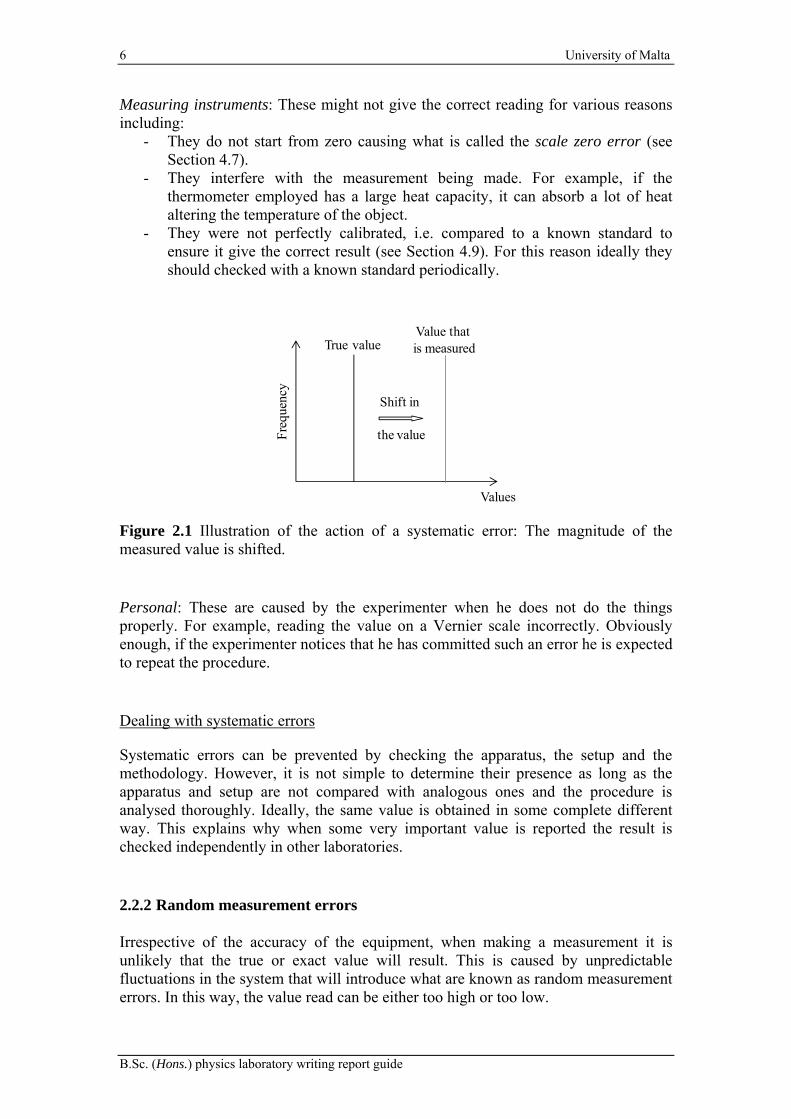
Systematic errors consist of a shift from the true value of the readings. They are caused by a bias in the measurement equipment that will not allow the correct value to be determined no matter how many times the experiment is repeated (see Figure 2.1).
Example 1: A metre ruler has been fabricated with a length of 98 cm. Each reading will be 2 % less than the correct value.
Example 2: When measuring the speed of a trolley, the distance between the light gates used to determine the time of travel is set to 47 cm instead of 50 cm.
Types of origin of the systematic errors
Apparatus: This is caused when the apparatus does not conform to the ideal conditions. For example, if a retort stand wobbles, it could move during the experiment causing a bias.
Method: This is caused when the method used is not in line with the parameters used to derive the governing equations. For example, if the oscillations of a simple pendulum are not small and planar then the conditions set when deriving the equations for simple harmonic motion would not be satisfied.
6 University of Malta
B.Sc. (Hons.) physics laboratory writing report guide
Measuring instruments: These might not give the correct reading for various reasons including:
- They do not start from zero causing what is called the scale zero error (see Section 4.7).
- They interfere with the measurement being made. For example, if the thermometer employed has a large heat capacity, it can absorb a lot of heat altering the temperature of the object.
- They were not perfectly calibrated, i.e. compared to a known standard to ensure it give the correct result (see Section 4.9). For this reason ideally they should checked with a known standard periodically.
Figure 2.1 Illustration of the action of a systematic error: The magnitude of the measured value is shifted.
Personal: These are caused by the experimenter when he does not do the things properly. For example, reading the value on a Vernier scale incorrectly. Obviously enough, if the experimenter notices that he has committed such an error he is expected to repeat the procedure.
Dealing with systematic errors
Systematic errors can be prevented by checking the apparatus, the setup and the methodology. However, it is not simple to determine their presence as long as the apparatus and setup are not compared with analogous ones and the procedure is analysed thoroughly. Ideally, the same value is obtained in some complete different way. This explains why when some very important value is reported the result is checked independently in other laboratories.
2.2.2 Random measurement errors
Irrespective of the accuracy of the equipment, when making a measurement it is unlikely that the true or exact value will result. This is caused by unpredictable fluctuations in the system that will introduce what are known as random measurement errors. In this way, the value read can be either too high or too low.
Shift in
the value
Value that is measured
Fre
quen
cy
True value
Values

Department of Physics 7
Chapter 2 Some basic concepts
Example 1: Variation in the dimensions of an object such as the diameter of a wire along the wire’s length. (In order to reduce production costs, some variation in the dimensions of mass produced goods is allowed.)
Example 2: The intensity of solar radiation can vary due to changes in solar activity, random changes in the composition and density of air etc.
Types of origin of the random measurement errors
Accidental: This is due to the inability of the set up to stabilize environmental condition. Examples include variation in draughts intensity and temperature fluctuations.
Personal: This is caused by a limit in observational capabilities of the experimenter. An example would be parallax error, which occurs when the value of a measurement depends on the line of sight (see Section 4.5).
Variation in quantities being measured: Such an error results due to the difficulty in obtaining and retaining uniformity in manufactured objects. An example would be the variation of the diameter of a wire along its length.
Scale rounding-of error: Any scale is accurate only up to a certain number of significant figures or decimal places. Thus, any reading involves the rounding (both up and down) of the values. An example of this type of error is provided by the case where all the readings were being taken using a micrometer screw gauge (that has a least count of 510 m) except for one that is taken using a metre ruler (that has a least
count of 310 m). In such a case, the error in the metre ruler will be much more significant than those of the others, a fact that should be pointed out. Note that such an error is often negligible when compared to others. In fact, instruments are usually chosen so that they provide comparable relative errors. As thus, this type of error should only be acknowledged if other sources of error are much less.
Dealing with random errors
Even though the magnitude of a random error is not in itself predictable, the frequency with which it occurs usually can be estimated using probability distributions. In fact, usually (but not always), random errors can be characterised by a normal (Gaussian) distribution. For a variable x, this distribution takes the form,
2
2
1exp ,
22
xf x
(1)
where is the mean or average and 2 the variance defined respectively by,

8 University of Malta
B.Sc. (Hons.) physics laboratory writing report guide
xf x dx
(2)
and
22
.x f x dx
(3)
Making a measurement is considered to be equivalent to sampling from such a distribution, with the true value being its mean (see Figure 2.2).
Figure 2.2 Illustration of what is meant by random error: Making a measurement is equivalent to sampling from some distribution (usually the Gaussian or normal distribution). There is an associated frequency with each possible measured value.
It is obvious that, provided the probability distribution is sufficiently symmetric, a better estimate of the true value can be obtained by averaging over a large number of observations. This follows from the fact that positive and negative biases will average out. As a matter of fact, the probabilistic nature of random error allows us to treat them using statistics. We will discuss this in more detail in Section 2.4.1.
2.2.3 Comparison between systematic and random measurement errors
Systematic and random errors have a number of features that can help us to discriminate between them. For ease of comparison, these have been listed in Table 2.1.
Fre
quen
cy
True value
Values
Different values can be measured with different probability
Measuredvalue

Department of Physics 9
Chapter 2 Some basic concepts
Systematic Errors Random Errors
- Consist of a bias in the system. - Consist of random fluctuations in the system.
- They are repeatable, i.e. averaging over repeated readings will not reduce them.
- They are not repeatable, i.e. they can be both higher and lower than the true value.
- They can only be contained by setting up the apparatus carefully, accurate calibration of the instrumentation and cross-comparison with known values.
- They can be contained by averaging repeating readings.
- It is difficult to study them statistically.
- Can be studied statistically.
Table 2.1 Comparison between systematic and random errors.
Figure 2.3 The error in every measurement is a combination systematic and random errors.
Finally, it should be noted that usually systematic and random errors do not occur in isolation. In practice, they combine to give a final error that is constituted by a random error around a systematic error as illustrated in Figure 2.3.
2.3 The uncertainty of a measured quantity
We will now discuss how we can quantify the uncertainty in a measurement or a calculated quantity. To do this, first we are going to consider how we should quote the value of a quantity.
Fre
quen
cy
True value
Values
Distribution of measurements
MeasuredvalueRandom
Error
Systematic error
Total error
Mean ofmeasurements

10 University of Malta
B.Sc. (Hons.) physics laboratory writing report guide
2.3.1 Quoting values
What would you understand if I told you that a table is 2 long? Would you be able to determine how long it is? The answer should be no, as we need to refer to some scale in order to determine how long that object is. We do so by adding a unit to the number such as meters or centimetres. This is indicative of the fact that in physics a quantity is not simply characterised by a number. We need at least a unit. Sometimes we also need a direction such as when we discuss displacements.
Possibly, you were already aware of these requirements. However, this is not enough. We also need to quantify how accurate the value is. In order to appreciate the importance of this, suppose that I were to tell you that I am 1.8 m long, plus or minus 1.5 m. This would mean that I am either a 30 cm dwarf or 3.3 m giant. Effectively by telling you my height, I gave you no useful information.
Thus apart from a value and a unit, a quantity needs to be quoted together with an uncertainty. For example, if we measure the length of a desk using a metre rule, and find that it is equal to half a metre then we can write,
0.500 ± 0.001 m.
You can see that apart from 0.500 m, I have included the uncertainty, ± 0.001 m, that is associated with the measurement. This depends on the measuring instrument, which in this case was a meter rule, so that the least scale reading, 1 mm, seems appropriate as an estimate of the uncertainty in the measurement. You should also note that the way in which I have written the length is consistent with the uncertainty, in that it has the same number of significant figures. This refers to a basic principle that applies when quoting measurements, namely that the value should always have the same number of significant figures or decimal places as the uncertainty, neither more nor less. Thus is would have been wrong to write values such as,
0.72 ± 0.001 m or 0.523567 ± 0.001 m.
The proper values to report are,
0.720 ± 0.001 m and 0.524 ± 0.001 m.
In the first case, I have padded with zeros while in the second I have rounded so that in both instances I have reported a value with three significant digits that is consistent with the uncertainty.
Another thing to consider is that in your work you will frequently encounter very large numbers like:
245,000,000,000
or very small numbers like,
0.000,000,0476
These numbers are not very nice to read and handle. Thus, a system was devised so as to write them in a more friendly way. This system involves shifting the decimal point

Department of Physics 11
Chapter 2 Some basic concepts
until it is placed after the first non zero digit and then multiplying by 10 raised to the power of the number of decimal places moved if the magnitude of the number has decrease and to the negative power of the number of decimal places moved if the magnitude of the number has increased. To illustrate the principle we are going to use the numbers above:
We have moved the decimal point 11 places and the original number changed from 245,000,000,000 to 2.45. In order to get back the original number we had to multiply by 10 to the power of 11.
In this case, we have moved the decimal point by 8 places so that the number changed from 0.000,000,0476 to 4.76. If we want back the original number we need to divide by 810 or multiply the resultant number by 810 .
When numbers are written as shown above, with a decimal point after the first significant figure and then multiply by 10 to some power, we say they are in standard form. Such numbers are easier to handle. For this reason, whenever appropriate, you should write the values in this format.
2.3.2 The uncertainty in a single measurement
Before proceeding any further, we will define a number of concepts. These definitions will be referred to continuously in what follows. Hence, you should spend some time learning them.
Some important definitions
The true value of a quantity is the value of that quantity free from any error. This is in general not available.
The measured value of a quantity is the value of that quantity as measured by some instrument. This is what we will have access to.
The absolute (or total) error is the difference between the true and the measured value. This is in general not available.
The uncertainty (or deviation) represents the variation in measured data. Numerically it gives an interval about the value measured inside which the true value should reside.
The least count is the smallest scale division that is marked on the instrument. It is also the least increment between successive values. For example, in the case of a meter ruler the least count is 1 mm.
The readability refers to the precision with which a scale can be read. This depends both on the least count as well as on the person doing the experiment. It can be
11245,000,000,000 2.45 10 .
80.000,000,0476 4.76 10 .

12 University of Malta
B.Sc. (Hons.) physics laboratory writing report guide
quantified as the smallest scale division that can be read by the experimenter. In this way, it provides the round off value.
The practical significance of some of these definitions might be obscure. So let us spend some time trying to explain them. It is likely that up till now you have been instructed to use the least count of an instrument as the smallest scale division that can be read from a scale. For example, when using a rule, you would probably have been instructed to round off your values at 1 mm, hence setting this value as the readability. You would also have been told that the “error” in the reading – more precisely, the uncertainty – is also equal to the least count. Once again, for a metre rule this would be 1 mm. However, the least count, the readability and the uncertainty are all distinct concepts and from now on, you are expected to distinguish between them.
Figure 2.4 An object being measured by a rule that is marked in centimetres.
To give you an example consider an object being measured by a ruler that is marked in centimetres as shown in Figure 2.4. The least count in the ruler is 1 cm. Obvious such space intervals are very course and if used to round values we can have a substantial difference between the actual length and the one measured. In fact, most people would agree that the object is about 7.5 cm long. In so doing, the readability of the rule has been set to at least 0.5 cm, which is half the interval between markings. Effectively most persons would have no difficulty using a readability of at least 0.25 cm on this ruler as they can easily judge in which quarter the edge of the object stands. Check out Figure 2.5 to see if you can get the length of A as 4.25 cm and that of B as 8.75 cm. Other persons might be able to divide such a scale reasonably accurately into ten. There is nothing wrong in doing so if it is within your abilities. For this reason, it will be left up to you to decide the smallest subdivision that you want to read from a scale, i.e. the readability. The only restriction is that you are reasonable in your choice.
Figure 2.5 Two object being measured by a rule that is marked in centimetres.
1 2 3 4 5 6 7 8 90 10
Object
Rule
1 2 3 4 5 6 7 8 90 10
A
Rule
1 2 3 4 5 6 7 8 90 10
B
Rule

Department of Physics 13
Chapter 2 Some basic concepts
Once you have decided what the readability should be, there is the issue of determining the associated uncertainty. This is meant to give a range of values within which the experimenter is sure that the measurable value is found. To illustrate the point, let us consider again the situation shown in Figure 2.4. For simplicity, let us assume that we measure the length of the object to be 7.5 cm. Referring to Figure 2.6, different experimenters may set the range of values where the measurable value lies differently. Some would simply say that the measureable value lies,
7.0 cm 8.0 cm,l
as indicted in Figure 2.6(a). In this way the length can be written as,
7.5 0.5 cm,l
where 7.5 cm is the average of the range and 0.5 cm is the uncertainty. However, others might be more confident in their abilities and be able to state that,
7.25 cm 7.75 cm,l
as indicted in Figure 2.6(b). This would be equivalent to stating that,
7.50 0.25 cm,l
where 7.50 cm is the average of the range and 0.25 cm is the uncertainty.
(a)
(b)
Figure 2.6 Different ways of defining the uncertainty in the length of an object measured with a rule that is marked in centimetres. In (a) the uncertainty is taken to be
0.5 cm while in (b) it is taken as 0.25 cm.
1 2 3 4 5 6 7 8 90 10
Object
Rule
Uncertainty taken to be 0.5 cm on each side of the reading
Measurement can lie in this range of possible values
1 2 3 4 5 6 7 8 90 10
Object
Rule
Uncertainty taken to be 0.25 cm on each side of the reading
Measurement can lie in this range of possible values

14 University of Malta
B.Sc. (Hons.) physics laboratory writing report guide
The question you are probably asking yourself at the moment is, who is right? The answer is both! The uncertainty in a measurement depends on the confidence of the person carrying out the experiment. Hence, there are no hard and fast rules. It all depends on the experimenter’s ability to determine a range of values within which he is confident that the measurable value is found. For this reason, it will be left up to you to determine the appropriate uncertainty for each measurement you take. Obviously this has to be meaningful.
As a guideline, in most cases the following order is followed,
Least count Readability Uncertainty.
However, this might not always hold. As an example, consider the situation where you try to measure the diameter of a ball using a straight stiff rule as shown in Figure 2.7. Since the ball is round, it is not possible to place both ends of the ball in contact with the rule at the same time. This automatically introduces a large parallax error in the reading, the magnitude of which depends on the ability of the experimenter. In such situations, the measurement should reflect the imposed limitation. Essentially this would mean that both the readability as well as the uncertainty are likely to be estimated to be larger than the least count of the rule, i.e. larger than 1 mm.
Figure 2.7 Measuring the diameter of a ball using a straight rule marked in millimetres.
Another example where the uncertainty in the measurement would be larger than the least count of the instrument occurs when the measurements involve the human reaction time (see Section 4.4). This occurs for example when you measure the periodic time of an oscillating system. In such a case, no matter how precise your stopwatch is, the uncertainty in the measurement should never be less than the average human reaction time, i.e. 0.3 s.
This is not as yet the end of the story. The uncertainty obtained as discussed before may need to be corrected for various factors including:
- Intrinsic tolerances: Instruments are calibrated so that for a given input they provide the corresponding outputs. This is carried out using known standards. However, it is not possible to calibrate for all possible inputs. Furthermore it is frequently not practical to be 100 % accurate in the calibration. This gives rise
Department of Physics 15
Chapter 2 Some basic concepts
to tolerances, which are nothing more than a range of values where the measured output should lie. Tolerances are usually expressed as percentage and can vary over the global range of an instrument. For example, a digital meter might have a tolerance of 3 % between 0 and 100 and 2 % between 100 and 1000. Thus, in order to obtain the uncertainty, the least count – which is also the readability in this case – should be multiplied by 1.03 if the reading is between 0 and 100 and 1.02 if it is between 100 and 1000 to in order to obtain the uncertainty. This provides an example of the uncertainty being larger than both the readability and the least count.
- Temperature fluctuations: The reading in an instrument can vary if the temperature changes. A simple reason for this is thermal expansion. They also affect significantly the performance of electronic circuits. For this reason, most instruments are provided with an optimal working range of temperatures. Corrections for the temperature can also be provided, most frequently for sophisticated instruments.
- Variation in gravity: Gravity changes on going from the equator to one of the poles. This could introduce uncertainties due to the variation of the local gravity.
While it would be good to keep these other factors in mind, for this course, you are not expected to take into account such corrections.
2.4 The uncertainty of a calculated quantity
In the previous section, we have seen how we can get the uncertainty in a measured quantity. However, most of the time we do not just use the measured quantity as it is. In practice, we manipulate the measurements arithmetically to determine other quantities.
Whenever we calculate something, the uncertainty in the measured quantities used are carried over to the quantity derived. Hence, we need a way to quantity the uncertainty in the calculated quantity. There are various method of how to do this. You might have already encountered some approximate methods that can be used to determine the number of significant figures with which your answers should be given. This would have followed from an estimate of the uncertainty in the final calculations. In this course, we will take a more formal approach that is based on statistics. At present, this is the prevalent way of determining the uncertainties. The maximum possible uncertainty will also be discussed.
2.4.1 The uncertainty in repeated readings of the same measurement
As mentioned in Section 2.2.2, due to random errors, making measurements is equivalent to sampling from some distribution. This is usually the normal distribution or can be approximated by it. Thus, it is possible to apply a type of statistical analysis known as hypothesis testing to obtain confidence intervals for the uncertainty in the measurement. A full analysis of such a subject would be too extensive to cover and is

16 University of Malta
B.Sc. (Hons.) physics laboratory writing report guide
far beyond the scope of this work. For this reason, only an outline of the methods used will be provided. The reader can refer to standard text books like Miller and Miller (1999) for a more comprehensive review.
Suppose we are given a normal population (Equation 1) with population mean
(Equation 2) and population variance 2 (Equation 3). Let us obtain a random sample (by making measurements) from this distribution, ,iX for 1,2,..., .i n We can then
define the sample mean X and the sample variance 2s of the random sample respectively by,
n
iin X
nXXX
nX
121
11 (4)
and 2
22 2
1 1 1
1 1 1,
1 1
n n n
i i ii i i
ns X X X X
n n n n
(5)
where the overbar indicated an averaging process and the upper case sigma Σ (Greek letter for S), is the symbol used for summation. A theorem in statistics then tells us that the variable,
,X
Ts n
(6)
has the t distribution with 1n degrees of freedom.
Figure 2.8 Schematic plot of the t distribution. The probability that , 1nT t can be
found by integrating from to , 1.nt This is equivalent to determining the area
under the graph that is not shaded in grey. The excluded area has a magnitude .
The t distribution is another probability distribution that resembles in shape the normal distribution. Like all distributions, we can get the probability of T being
f(t)
t, 1nt
The t distribution
Shaded area , 1
This area represents the probably that in a measurement nT t

Department of Physics 17
Chapter 2 Some basic concepts
smaller or equal to some value , 1nt by calculating the area under the graph between
minus infinity and , 1.nt Mathematically this can be written as,
, 1
, 1
1 .nt
nP T t f t dt
(7)
This is schematically illustrated in Figure 2.8. As indicated in the figure, the excluded area is assumed to have a magnitude , i.e.,
, 1
,
ntf t dt
(8)
This explains the origin of the subscript used for , 1.nt (Note 1n gives the
number of degrees of freedom usually denoted by the symbol . )
Note that for probability distributions the total area under the graph is one, representing a certainty. Thus, the quantity 1 give us a measure of the level of certainty of the result. For example, if we want to be 90 % confident that a measured value of T is smaller or equal to , 1nt then we need to choose as,
901 90 % 1 0.10.
100 (9)
In general, for any level of confidence (LoC) we choose as,
LoC1 ,
100 (10)
where it is being assumed that the level of confidence is given as a percentage. We can then work out the value of , 1nt that would give us such confidence using
Equation 7. This will require numerical methods that are covered elsewhere in the physics degree.
At this point, we are in a position to write down an expression for the uncertainty in the sample average X where we are confident that should lie. Combining Equations 6 and 7, the required equation is given by,
, 1 , 1 1 2 ./
n n
XP T t P t
s n
(11)
This expression might be puzzling, so let us try to explain how it arises. First of all, we have used the absolute value since X can be both greater as well as smaller than
. Thus if we open up the expression we get,

18 University of Malta
B.Sc. (Hons.) physics laboratory writing report guide
, 1 , 1
, 1 , 1
, 1 , 1
1 2/
1 2
1 2
n n
n n
n n
XP t t
s n
s sP t X t
n n
s sP X t X t
n n
, 1 , 1 1 2 .n n
s sP X t X t
n n
(12)
In other words the above expressions tells us that the probability of finding (which
represents the measurable value) in the interval 1/2, 1nX t sn
is given at a level of
confidence of 1 2 . The area under the graph that represents this probability is shown in Figure 2.9. This same figure also explains the factor of 2 that is associated with in the level of confidence: In our case we are interested in determining T between a range of value. Thus, we need to exclude two parts of the graph, one on the extreme right and one on the extreme left, what is referred to as a two tailed test. Given the symmetry of the t distribution these are located at , 1nt where , 1nt is
defined in Figure 2.8.
Figure 2.9 Schematic representation of the probability that is found in the given
interval, 1/2 1/2, 1 , 1, .n nX t sn X t sn
The level of confidence is 1 2 .
At this point, we need to determine an appropriate value for the level of confidence in the uncertainty. Obviously, the smaller the more we are confident that the measurable value is within the given interval. At the same time as decreases the uncertainty interval increases exponentially. Thus, we need to make a trade off in the chosen value of . A good cut off point, that is widely adopted in this type of work, is the 95 % level of confidence, giving 0.025 for a two tailed test. Values of
0.025, 1nt for different values of n, where n is the number of repeated readings, are given
in Table 2.2.
f(t)
t, 1nt
, 1
Area represents
/n
XP t
s n
, 1nt

Department of Physics 19
Chapter 2 Some basic concepts
n 2 3 4 5 6 7 8 9 10
0.025, 1nt 12.7 4.30 3.18 2.78 2.57 2.45 2.36 2.31 2.26
Table 2.2 Values of 0.025, 1nt for different values of the number of repeated readings n.
To summarise our findings, the uncertainty in the average value of the repeated readings ,X that is denoted by Δ ,X can be expressed as,
, 1Δ ,n
sX t
n (13)
where s, the square root of the sample variance (Equation 5), which is referred to as the sample standard deviation. This can be calculated from,
2
1
1.
1
n
ii
s X Xn
(14)
The values of , 1nt can be obtained from Table 2.2 while n is the number of repeated
readings. Note that as n increases the uncertainty goes to zero due to the factor of 1/2.n Let us now see how it works with an example.
Example: A student measures the width w of a bar at different points using a metre rule. His results are shown in the table below. Use them to determine a value for the average thickness.
/ mw 0.001 0.029 0.030 0.032
Comments: Before solving the problem, let us discuss the format of the table:
- The first column gives us the symbol and tells us that the values are all in metres.
- The second column is telling us that the values have an uncertainty of 0.001 m.
- The other columns tell us the values read. They have the same number of significant figures as the uncertainty in order to be consistent. This meant that in the case of column four, we had to pad with zeros.
- From the previous points, we can conclude that the readings taken were, 0.029 0.001 m, 0.030 0.001 m and 0.032 0.001 m. The table format is thus being used to avoid useless repetition of the units and the uncertainties.
This constitutes a standard layout and interpretation for such a table. We will have more to say about representation of measurements as we go along.

20 University of Malta
B.Sc. (Hons.) physics laboratory writing report guide
Solution: The average value is given by,
1
1 10.029 m 0.030 m 0.032 m 0.03033 m.
3
n
ii
w wn
This value is incomplete without the associated uncertainty. First, we need to determine the sample standard deviation,
2
1
2 2 2
1
1
10.029 m 0.03033 m 0.030 m 0.03033 m 0.030 m 0.03033 m
20.00153 m.
n
ii
s X Xn
In this way, the uncertainty interval can be determined from,
, 1Δ .n
sw t
n
Using 3n we find from Table 2.2 that 0.025,3 4.30.t Substituting values we get,
0.00153 mΔ 4.30 0.004 m.
3w
We can thus write the average value as,
0.030 0.004 m Ans.w
Comments: Before proceeding it is worth making a couple of comments,
- The uncertainty was provided even if we were not specifically asked for it. This is due to the fact that a value without an uncertainty is meaningless.
- The uncertainty obtained was rounded up to one significant figure. It does not make sense to specify the uncertainty to a large number of significant figures as the leading term should suffice. (Only in extremely accurate experiments is this rule not followed and the uncertainty is quoted to two significant figures).
- Even if during the calculations a large number of significant figures were retained, the final answer was given up to the uncertainty that was calculated. Padding with zero was carried out as necessary.
- Units were retained during the calculations. This is not strictly necessary. However, it serves as a consistency check. Basically the procedure builds on the homogeneity of equations that you should have covered at advanced or intermediate physics. It helps to identify mathematical errors by ensuring that the final answer has the expected units.

Department of Physics 21
Chapter 2 Some basic concepts
2.4.2 The uncertainty in a variable that is a function of other variables
In many instances, the quantity that we want is calculated through arithmetic manipulation of a number of different quantities each of which has an associated uncertainty. The uncertainty in the variables used will propagate into the final result giving an uncertainty in its value. There are various ways that can be used to estimate the uncertainty in the final answer. In this section, we are going to discuss the method that you are going to use in the laboratories. The formal derivation of the propagation of uncertainties is beyond the scope of this course. The interested reader can find a not too technical derivation in Chapter 4 of Squires (2001).
Let z be a function of n variables, 1 2, ,... ,nx x x i.e. 1 2, , , .nz f x x x Then it can be
shown that the uncertainty in z is related to that of the ix ’s, i.e. ,ix through the
equation,
2 2 2 2
2
1 211 2
Δ Δ Δ Δ Δ ,n
n iin i
z z z zz x x x x
x x x x
(15)
where,
,i
z
x
(16)
is the partial derivative of z with respected to .ix This is nothing more than the
derivative of z with respect to ix keeping all the other jx ’s, where ,j i constant.
As stated in Equation 15, the uncertainty in z might not be straight forward to calculate. For this reason, the equations to use for a number of common cases are listed below.
axz Δ Δz a x (17)
z ax by 22Δ Δ Δz a x b y (18)
xyz or y
xz
2 2Δ Δ Δz x y
z x y
(19)
pxz Δ Δz x
pz x (20)

22 University of Malta
B.Sc. (Hons.) physics laboratory writing report guide
xz ln Δ
Δx
zx
(21)
xez Δ Δz z x (22)
where x , y and z are variables while a , b and p are constants.
Proofs of the relations given by Equations 17 to 22 can be obtained by applying Equation 15. For example, Equation 19 can be obtained as follows. Assuming xyz then it follows that,
zy
x
and ,
zx
y
where in the first equation we have kept y constant and differentiated with respect to x while in the second we have kept x constant and differentiated with respect to y.
Substituting in Equation 15 gives,
2 22
2 2
Δ Δ Δ
Δ Δ
z zz x y
x y
y x x y
Dividing throughout by 2z keeping in mind that z xy we get,
2 2 2
2 2 2
Δ Δ Δ
Δ Δ Δ,
z y x x y
z xy xy
z x y
z x y
which is the desired result.
Repeating for 1z xy we get,
1zy
x
and 2.z
xyy
Substituting in Equation 15 gives,
2 22
2 21 2
Δ Δ Δ
Δ Δ
z zz x y
x y
y x xy y

Department of Physics 23
Chapter 2 Some basic concepts
Dividing throughout by 2z keeping in mind that 1z xy we get,
2 22 1 2
1 1
2 2 2
Δ Δ Δ
Δ Δ Δ,
z y x xy y
z xy xy
z x y
z x y
which again is the desired result.
Other situations can be easily obtained from the cases listed in Equations 17 to 22. For example if qp yxz then it follows from Equation 20 that,
1Δ Δ
ppx p x x and
1Δ Δ .
qqy q y y
At this point, we can use Equation 18 to obtain,
2 21 1Δ Δ Δ .p qz px x qy y
Of particular interest are the following results,
n
iii xaz
1
22
1
Δ Δn
i ii
z a x
(23)
n
i
ai
an
aa in xxxxz1
2121
22
1
ΔΔ ni
ii i
xza
z x
(24)
where large caption Π (Greek letter for P), is the symbol used for multiplication. The first relation can be obtained by repeated application of Equation 18 and the second one by the repeated and joint application of Equations 19 and 20. (Obviously, they can also be directly obtained from Equation 15.) Both situations occur frequently, so that it is good to keep these relations in mind. At this point, we are going to see some examples.
Example 1: In an experiment to determine the pressure P of a system, the height of a mercury column was found to be 0.010 0.001 m. Given that the density of mercury
is 313,534 kg m and the acceleration due to gravity is 29.81 m s determine the value
of the pressure. You can assume that P h g and that only h has an uncertainty.
Solution: 3 20.010 m 13,534 kg m 9.81 m s 1327.69 Pa.P h g
Using Δ Δz ax z a x we find the uncertainty of P as,
3 2Δ Δ 13,534 kg m 9.81 m s 0.001 m 100 Pa.P g h

24 University of Malta
B.Sc. (Hons.) physics laboratory writing report guide
Thus the answer can be given as,
1,300 100 Pa Ans.P
Example 2: The intensity I from a bulb at a point that is at a distance d depends on the power P through the equation,
243
.P
Id
A student measures the intensity at a point 1.000 0.001 m.d Given that the bulb has a power of 60.0 0.1 WP determine the value that the student should obtain. You can assume that the measuring instrument is ideal.
Solution:
2224 4
3 3
60.0 W14.324 W m .
1.000 m
PI
d
We now need to calculate the uncertainty. From Δ Δz ax z a x we get,
243
1Δ Δ .
PI
d
At this point we can use,
1 2
22
1 211
ΔΔ ,n i
n na aa a in i i
ii i
xzz x x x x a
z x
to determine 2Δ /P d as,
2 2 22
2
2 2 22
2
2 2 2
2 2
2 2
2 2
Δ / Δ Δ1 2
/
Δ / Δ Δ2
/
Δ ΔΔ 2
Δ ΔΔ 2 .
P d P d
P d P d
P d P d
P d P d
P P P d
d d P d
P P P d
d d P d
Substituting back we get,

Department of Physics 25
Chapter 2 Some basic concepts
2 2
2 24 43 3
1 1 Δ ΔΔ Δ 2 .
I
P P P dI
d d P d
This can be simplified to,
2 2Δ Δ
Δ 2 .P d
I IP d
Evaluating this expression gives,
2 22 20.1 W 0.001 m
Δ 14.324 W m 2 0.4 W m .60.0 W 1.000 m
I
The measurement the student should make is given by, 114.3 0.4 W m Ans.I
Example 3: Assume that a quantity can be expressed in terms of the variables P, a and Q through the equation,
4
8
Pa
Ql
where l is some constant. Determine an expression for the uncertainty in using those in P, a and Q. (Note that you have a very similar situation in one of the worksheets. However, in that case l also has an uncertainty.)
Solution: Using Δ Δz ax z a x we get,
4
Δ Δ .8
Pa
l Q
At this point we can apply the following relation to give us,
1 2
22
1 211
ΔΔ .n i
n na aa a in i i
ii i
xzz x x x x a
z x
This allows us to determine 4Δ /Pa Q as,
2 2 2 24
4
2 2 2 2424
Δ / Δ Δ Δ4 1
/
Δ Δ ΔΔ / 4
Pa Q P a Q
Pa Q P a Q
Pa P a QPa Q
Q P a Q

26 University of Malta
B.Sc. (Hons.) physics laboratory writing report guide
2 2 24 4 Δ Δ ΔΔ 4 .
Pa Pa P a Q
Q Q P a Q
Substituting back,
4
2 2 24
2 2 2
Δ Δ8
Δ Δ Δ4
8
Δ Δ Δ4 Ans.
Pa
l Q
Pa P a Q
l Q P a Q
P a Q
P a Q
Comparing the previous result with the one above, a pattern should become apparent.
2.4.3 The maximum uncertainty
In the previous section, we have used the variation of the measured quantities to determine the uncertainty. This gives us a good estimate of what the uncertainty should be. However, at times we are interested in the worst case scenario where the errors simply add up. This gives rise to the maximum uncertainty. Using calculus, an equation for the maximum uncertainty for 1 2, , , nz f x x x can be obtained as,
1 211 2
.n
n iin i
z z z zz x x x x
x x x x
(25)
where X is the maximum uncertainty in the variable X. For measured quantities, this is taken to be equal to the uncertainty in the measurement.
Equation 25 can be used to determine a number of special cases, much like we have done in the previous section. However, the matter is not perused to any further detail here. It is left up to the interested reader to follow it up.
2.5 The precision and accuracy of an experiment
Some important definitions
The precision relates the uncertainty to the measurement being taken. The smaller the uncertainty the better is the precision.
The accuracy describes how close the measured value is to the true value. The closer the measured value is to the true value the better is the accuracy.

Department of Physics 27
Chapter 2 Some basic concepts
Note that an experiment can be precise but due to the systematic errors involved it might not be accurate at all. On the other hand, it is also possible to have an accurate experiment that is not precise. This latter possibility is rather unlikely and depends mainly on chance.
It should be obvious that the importance of the magnitude of an uncertainty is related to that of the associated value. For example, if there is an uncertainty of 1 m in the measurement of 1 km then the measurement can be considered to be precise. However, if we have an uncertainty of 1 m in a measurement of 2 m, then the measurement cannot be considered to be precise.
In order to quantify the significance of the uncertainty with respect to the experimental determined value, the relative percentage error, defined as,
Combined ErrorPercentage error 100 %
Experimental Value (26)
can used. The percentage error is thus a measure of the precision and its value should be less than 10 % for the experiment to be considered as precise. Obviously, the closer to zero the percentage error is, the more precise is the experiment.
Another relative error that is of outmost importance is that relating the experimental value to the standard quotable one that is available from textbooks. A measure of this can be obtained from,
Experimental ValuePercentage accuracy 1 100 %.
Quoted Value
(27)
As its name implies, this quantity is a measure of the accuracy. Its minimum value is attained at zero, when the experimental and quoted value would be the same. This is indicative of the maximum accuracy. In order for an experiment to be considered as accurate, the percentage accuracy as defined above should be in the range of ±10 %. The best accuracy is attained when the percentage accuracy is 0 %.
Note that the percentage accuracy can also be defined as,
Experimental ValuePercentage accuracy 100 %.
Quoted Value (28)
In this case the best accuracy is obtained at 100 % so that an accurate experiment will be one where the experimental value is between 90 % and 110 % of the quoted value. Both definitions will be accepted provided the interpretation is correct. Let us now consider an example.
Example: A student carries out an experiment to determine the acceleration due to gravity and obtains a value of 210.9 0.1 m s . Determine if the experiment was precise and accurate.

28 University of Malta
B.Sc. (Hons.) physics laboratory writing report guide
Solution: To determine if the experiment was precise first we need to calculate the percentage error. This is obtained as,
2
2
Combined ErrorPercentage error 100 %
Experimental Value
0.1 m s100 %
10.9 m s0.92 %.
Since the percentage error is less than 10 % we can conclude that the experiment was precise.
To determine if the experiment was accurate, we need to determine the percentage accuracy. From standard tables we know that the value for the acceleration due to gravity is 29.81 m s . Hence the percentage accuracy is,
2
2
Experimental ValuePercentage accuracy 1 100 %
Quoted Value
10.9 m s1 100 %
9.81 m s11 %.
We see that the experimental value overestimates the quoted value by 11 %. This is more than 10 %. Hence, we can conclude that the experiment was not accurate.
The situation just discussed provides an example where the experiment was precise but not accurate.
2.6 Linear regression
2.6.1 Introduction
As discussed in the introductory part, we perform experiments to check how well our theoretical predictions conform to the real world. In general, this is carried out by comparing the values obtained to some equation derived from theory. While in principle it is possible to compare measurements using any type of equation, in practice, it is hard to determine the level of agreement if a general curve is used. On the other hand, it is very easy to establish whether the measurements follow a straight line, and how accurately they abide by this behaviour. For this reason, wherever possible, in physics data analysis is carried out using straight-line graphs. The problem then lies in the determination of the best straight line.
In the data analysis you have carried out so far, you have probably drawn the best straight line manually. To do this, you have been given guidelines on the procedure to follow. However, no matter how good the procedure you have adopted and how carefully you have applied it, there is always some element of subjectivity when using a manual procedure. For this reason, statistical techniques have been developed to

Department of Physics 29
Chapter 2 Some basic concepts
provide us with good estimates of the gradient and the intercept of a straight line from the experimental data.
The branch of statistics that deals with the linear modelling of a relation between two variables is called linear regression. Some of the basic aspects of the techniques involves will be discussed in what follows.
2.6.2 Determining the best straight line using the least square method
The process of drawing the best straight line can be described as a data fitting exercise. Thus, it is necessary to establish some criteria that would allow us to determine a good fit. In such situations, the method chosen in general requires the minimisation of the differences between the experimentally derived points and the line. This is embodied in the method of least squares.
Let us see how this algorithm works. Consider the set of points ,i ix y with
1,2,...,i n such as those shown in Figure 2.10. In principle, these points exhibit a linear trend. However, there are significant fluctuations around their main behaviour. These deviations can be quantified as the vertical difference of the point from the straight line. Referring to Figure 2.10, the magnitudes of the difference are given by the length of the grey lines (both solid as well as dotted). The idea behind the method of least squares is to minimise the sum of the magnitudes of these differences, or equivalently the total length of the grey lines.
Figure 2.10 Schematic representation of how the best straight line minimises errors over different readings. The vertical grey lines represent the deviations from the line of best fit.
y
x
Line of best fit
Plottedpoints
Overestimation
Underestimation

30 University of Malta
B.Sc. (Hons.) physics laboratory writing report guide
To set the situation in mathematical terms, let m and c be respectively the gradient and the intercept of the best straight line. Then the error for point , ,i ix y also referred to
as the residual, is given by,
,i i ie y mx c (29)
where imx c gives the value of y on the straight line when .ix x We now square
all the errors and sum to obtain the residual sum of squares,
22Res
1 1
.n n
i i ii i
S e y mx c
(30)
The reason why we have squared before we summed is that we want to minimize the magnitudes, i.e. the total differences, without having negative and positive divergences compensating for each other. In such situation, it is easier to work with the square rather than with the modulus (or absolute value). For this reason, squaring the differences to get an estimate of the deviations is a very common procedure adopted in statistics.
We now want to determine the values of m and c that would minimise Res.S We know
from calculus that to minimise we need to differentiate and set the result equal to zero. Since ResS is a function of both m and c we need to take the partial derivatives (see
Equation 16). This would yield the conditions,
Res
1
0n
i i ii
Sx y mx c
m
(31)
and Res
1
2 0.n
i ii
Sy mx c
c
(32)
Note that the last condition implies that minimising values of m and c have to be such that the sum of the residuals, i.e. the ie ’s, should be zero, i.e. the straight line ensured
the positive and the negative deviations cancel each other. Referring to Figure 2.10, this is equivalent to requiring that the length of the solid grey lines (over predictions) and that of the dotted grey lines (under predictions) are equal. You might recall this as a guiding criteria that you have been given to draw the best straight lines manually.
Equations 31 and 32 are two coupled equations with two unknowns. Thus, they can be solved for the gradient and the intercept using standard techniques. Going through the algebra, the following relations are obtained,
xy
xx
Sm
S (33)

Department of Physics 31
Chapter 2 Some basic concepts
and .c y mx (34)
where,
1
1,
n
ii
x xn
(35)
1
1,
n
ii
y yn
(36)
2
2 2
1 1 1
1n n n
xx i i ii i i
S x x x xn
(37)
and 1 1 1 1
1.
n n n n
xy i i i i i ii i i i
S x x y y x y x yn
(38)
Equations 33 and 34 are thus our best estimates respectively for the gradient and the intercept. The problem now lies in determining the uncertainties in these quantities. This will be tackled in the next section.
2.6.3 The uncertainties in the gradient and the intercept
The expressions that we have obtained for the gradient and the intercept are not the true values. They are only good estimates of the true value. To see this just consider that the residuals ie (Equation 29) in general are not zero. In practice, this is
unavoidable due to the presence of random errors. Thus, as we discussed in Section 2.4.1, when we make a measurement of y what we are really doing is sampling from some distribution.
To solve the problem, it can be assumed that the conditional probability density function of iy for a given ix denoted by |i iw y x is given by the normal density i.e.
2
2
1| exp ,
22
i i
i i
y mx cw y x
,iy (39)
where m, c and are constants and do not change with i. Here, m and c are simply
the gradient and the intercept, while 2 is the variance defined by (Equation 3),

32 University of Malta
B.Sc. (Hons.) physics laboratory writing report guide
22
,X f X dX
(40)
where X is a general variable, f X is its probability density distribution and is the population mean.
A pictorial picture of the situation is given in Figure 2.11. The true (correct) values of y at a point ix are given by .i iY mx c The values of the iY lie on the true line. In
practice, due to random errors, when a measurement it made iy results. The
distribution of iy around the true value iY is being assumed to be a normal
distribution.
Figure 2.11 Pictorial representation of the conditional probability density function of .iy The i iY mx c represent the true value that should be obtained when .ix x
However, due to random errors, the value obtained for y is .iy The distribution of iy
around the true value iY is assumed to be a normal distribution.
The practical significance of the variance is that it gives us a measure of the spread of the possible values that can be sampled. This should transpire clearly from its own definition (Equation 40), that gives the variance as the average of the squares of the deviations from the mean. Furthermore, considering its square root, , called the standard deviation, it can be shown that most of the probability, around 68.2 %, lies
in interval , as shown schematically in Figure 2.12. Given that the mean
of the distribution is equivalent to the measurable value (see Section 2.2.2), it can be concluded that is a measure of the uncertainty in the measurements.
y
x
1Y
1x 2x 3x
2Y
3Y

Department of Physics 33
Chapter 2 Some basic concepts
Figure 2.12 Schematic illustration of the properties of the standard deviation for a Gaussian distribution. Most of the probability is contained between and . Returning to Equation 39, this distribution tells us that if we make a measurement of
iy at the point ix then the values of iy that we can obtain will have a normal
distribution around the mean value given by .imx c From the previous discussion, a
measure of the uncertainty with which we are measuring iy is given by the standard
deviation . Now to calculate m and c we are using the measured values of iy that
will have an uncertainty associated with them. As a result, the uncertainty in the iy
will propagate to the values of m and c as discussed in Section 2.4.2.
The detailed derivation of the resultant uncertainty in the gradient and the intercept is beyond the scope of this course. The interested reader can find a simple derivation in books like Squires (2001) or Taylor (1997). A more detailed statistical treatment can be found in Miller and Miller (1999). Going through the mathematics the standard errors in the gradient and the intercept are found to be,
2
1Δ 1
2
mm
rn
( 41)
and 2
1
1,
n
ii
c m xn
( 42)
where r is called the correlation coefficient and can be expressed as,
,xy
xx yy
Sr
S S ( 43)
with,
2
2 2
1 1 1
1.
n n n
yy i i ii i i
S y y y yn
(44)
The physical significance of r will be discussed in the next section.
Frequency
X
Probability the value sampled is from the non-shaded region is
68.2 %
Probability the value sampled is from this shaded region
is 15.9 %

34 University of Malta
B.Sc. (Hons.) physics laboratory writing report guide
2.6.4 Covariance and correlation
So far we have found a way of determining the best estimates of the gradient and the intercept for a set of data. This procedure can be carried out for any set of data, even if a straight line does not describe the points accurately! Thus, a natural question arises: How well does the straight line describe the variation of one variable with the other?
One way to measure how the values of iy vary with those of ix (and vice versa) is to
use the covariance, that for a set of n points can be defined as,
1 1 1 1
1 1 1 1.
n n n nxy
xy i i i i i ii i i i
Sx x y y x y x y
n n n n n
(45)
Let us see why this should be so. If the occurrence of large values of iy ( y ) occur
with large values of ix ( x ) then the value of xy would be positive. The same holds
if small values of iy ( y ) occur with small values of ix ( x ). Thus, positive xy
indicates that the values of iy and ix increase and decrease together.
Consider now the situation where large values of iy ( y ) coincide with small values
of ix ( x ). Then xy would be negative. The same would occur if small values of iy
( y ) occur with large values of ix ( x ). Thus, negative xy would indicate that iy
and ix have opposite tendencies, when one increases the other decreases.
Finally, in the case that the magnitudes of the iy ’s and those of the ix ’s are
completely independent, then xy should approach zero as n goes to infinity. The
reason for this is that for any value of iy and y the quantity ix x is equally likely
positive as it is to be negative. Thus, on average the positive contribution will cancel out with the negative contributions, meaning that xy will approach zero. Whenever
this happens, and 0,xy we say that ix and iy are uncorrelated – this is actually
different from saying that they are independent.
The problem with xy is that its magnitude cannot be directly related to how well the
variables move together or in opposite directions. You can see this by considering that a simple change in units would be enough to change the value of ,xy even if the set
of points stays the same. However, it can be shown (using the Schwarz inequality) that,
xy x y (46)
where x and y are respectively the (population) standard deviations of ix ’s and
iy ’s given as,

Department of Physics 35
Chapter 2 Some basic concepts
2
2 2
1 1 1
1 1 1n n nxx
x i i ii i i
Sx x x x
n n n n
(47)
and 2
2 2
1 1 1
1 1 1.
n n nyy
y i i ii i i
Sy y y y
n n n n
(48)
For this reason, a measure of how much two quantities depend linearly on each other can be defined as,
1
2 2
1 1
.
n
i ixy xy i
n nx y xx yy
i ii i
x x y yS
rS S
x x y y
( 49)
This can also be expressed as,
1 1 1
2 2
2 2
1 1 1 1
1 1 1
.1 1 1 1
n n n
i i i ii i i
n n n n
i i i ii i i i
x y x yn n n
r
x x y yn n n n
( 50)
The quantity r is called the (Pearson) correlation coefficient. It is evident from the fact that xy x y (Equation 46) that its values range from 1 to 1. We will now show
that the maximum and minimum values are attained when the iy ’s depend linearly on
the ix ’s.
Consider the particular situation when the iy ’s are linearly dependent on the ix ’s so
that they can be expressed as .i iy mx c It would immediately follow that,
1 1
1 1.
n n
i ii i
y y mx c mx cn n
( 51)
In this way,
.i i iy y mx c mx c m x x ( 52)
Substituting in the equation for r (Equation 49) gives,

36 University of Malta
B.Sc. (Hons.) physics laboratory writing report guide
1
2 2
1 1
1
2 22
1 1
2
1
2 2
1 1
n
i ii
n n
i ii i
n
i ii
n n
i ii i
n
ii
n n
i ii i
x x y yr
x x y y
x x m x x
x x m x x
m x x
m x x x x
or .m
rm
( 53)
Hence, the possible values of r for this case are 1 depending on the sign of the gradient m. This conclude the proof that the maximum and minimum values occur when possible values iy ’s depend linearly on the ix ’s.
From this result we can infer that the closer to one r is, the more we are certain that
iy and ix vary linearly and hence their relation can be described by a linear equation.
In practice, it is unlikely that in an experiment we get a value of 1r even if the variables are linearly dependent. The reason can be found in the random errors present in any set up.
Now consider the situation where the variables are independent then 0xy (see
discussion following Equation 45). Since xy is in the denominator of r then it would
follow that 0,r indicating that the variables are uncorrelated. Thus the smaller the value of r the more we are sure that there is no linear relation between the variables.
At this point, you should note that if the iy ’s are equal to a constant, Equation 53
would lead to 0 / 0r since the gradient is zero. The result would then be undefined. If we estimate r from a sample, then the outcome would depend on the errors. For this reason, the correlation coefficient should not be used in cases where we know that the gradient is zero or very small.
Finally, the correlation coefficient can be used to determine how much of the variation of y is explained by that of x. The detailed derivation is beyond the scope of this work. A quantitative approach is given in Taylor (1997) while a complete statistical treatment can be found in Miller and Miller (1999). In essence, the quantity,
2 100 %,r (54)

Department of Physics 37
Chapter 2 Some basic concepts
gives the percentage of the total variation of y that can be explained through the linear relation with x. Thus, for example, if 0.9r then 81 % of the total variation of y can be explained through the linear equation.
2.6.5 The coefficient of determination
Another way of quantifying how accurately the points follow a straight line is given by the coefficient of determination, denoted by 2,R and calculated as,
2
2 Res 1
2
1
1 1 .
n
i ii
nyy
ii
y mx cS
RS y y
(55)
Using the fact that /xy xxm S S and ,c y mx we can show that the coefficient of
determination in the case of linear regression is equal to the correlation coefficient square. This can be done as follows,
2
2 1
2
1
2
1
2
1
1
n
i ii
n
ii
nxy xy
yy i ii xx xx
yy
nxy
yy i ii xx
yy
yy
y mx cR
y y
S SS y x y x
S S
S
SS y y x x
S
S
S
2
iy y
22
21
2
21
2
2
xy
nxy xy
i i ii xx xx
yy
S
nxy xy
i iixx xx
S Sy y x x x x
S S
S
S Sy y x x
S S
2
1
n
ii
x x
2 2
2
2
yy
xy xy
xx xx
yy
xy
xx yy
S
S S
S S
S
S
S S
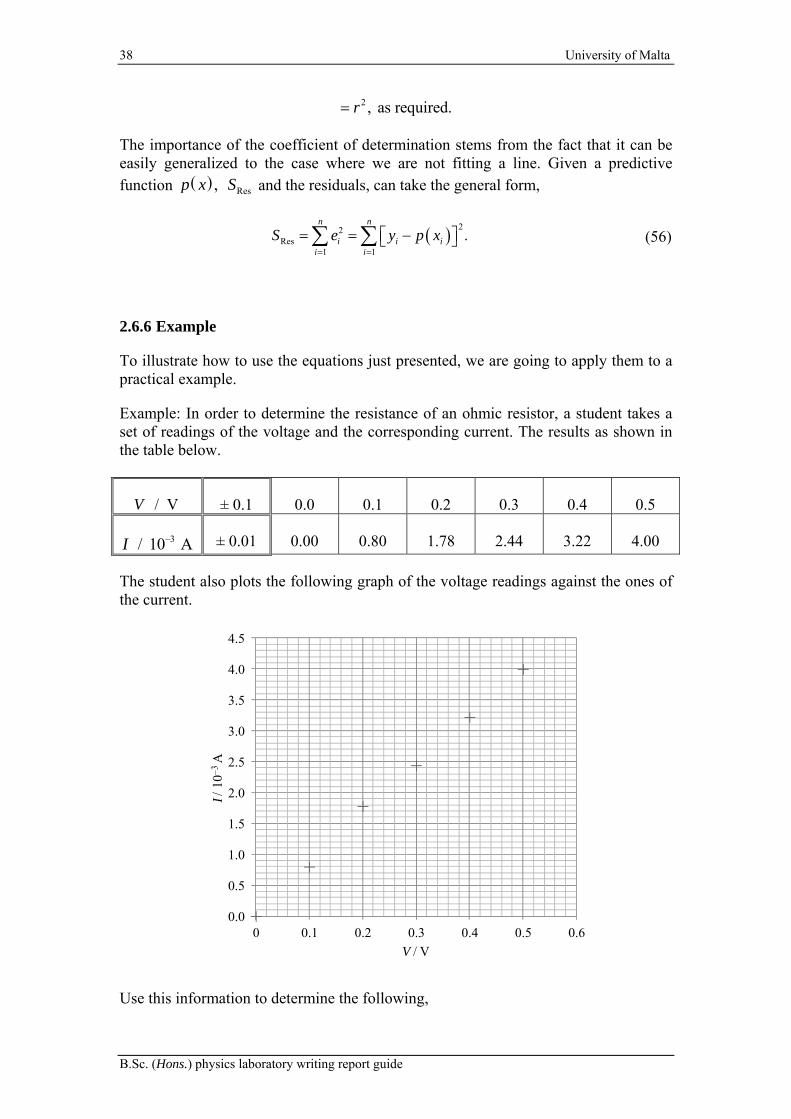
38 University of Malta
B.Sc. (Hons.) physics laboratory writing report guide
2 , as required.r
The importance of the coefficient of determination stems from the fact that it can be easily generalized to the case where we are not fitting a line. Given a predictive function ,p x ResS and the residuals, can take the general form,
22Res
1 1
.n n
i i ii i
S e y p x
(56)
2.6.6 Example
To illustrate how to use the equations just presented, we are going to apply them to a practical example.
Example: In order to determine the resistance of an ohmic resistor, a student takes a set of readings of the voltage and the corresponding current. The results as shown in the table below.
/ VV ± 0.1 0.0 0.1 0.2 0.3 0.4 0.5
–3 / 10 AI ± 0.01 0.00 0.80 1.78 2.44 3.22 4.00
The student also plots the following graph of the voltage readings against the ones of the current.
Use this information to determine the following,
0.0
0.5
1.0
1.5
2.0
2.5
3.0
3.5
4.0
4.5
0 0.1 0.2 0.3 0.4 0.5 0.6
I/ 1
0–3A
V / V

Department of Physics 39
Chapter 2 Some basic concepts
(a) Values for the gradient and the intercept. (b) The error in the gradient and the intercept. (c) Find a value for the resistance R of the ohmic resistor.
Solution:
It is clear from the data and the graph that we can take ii Vx and .i iy I The
number of data points n = 6.
For ease of reference, we are first going to work out a number of quantities that we need for our calculations. Basically, the summations we need:
6 6
1 1
0.0 V 0.1 V 0.2 V 0.3 V 0.4 V 0.5 V 1.5 V.i ii i
x V
6 6
2 2 2 2 2 22 2
1 1
2
0.0 V 0.1 V 0.2 V 0.3 V 0.4 V 0.5 V
0.55 V .
i ii i
x V
6 63 3 3
1 1
3 3 3
3
0.00 10 A 0.80 10 A 1.78 10 A
2.44 10 A 3.22 10 A 4 10 A
12.24 10 A.
i ii i
y I
6 6 2 2 22 2 3 3 3
1 1
2 2 23 3 3
6 2
0.00 10 A 0.8 10 A 1.78 10 A
2.44 10 A 3.22 10 A 4 10 A
36.1304 10 A ,
i ii i
y I
6 63 3
1 13 3
3 3
0.0 V 0.00 10 A 0.1 V 0.80 10 A
0.2 V 1.78 10 A 0.3 V 2.44 10 A
0.4 V 3.22 10 A 0.5 V 4.00 10 A
i i i ii i
x y V I
3 4.456 10 V A,
6
1
1 1.5 V0.25 V.
6ii
x V Vn
363
1
1 12.24 10 A2.04 10 A.
6ii
y I In
2
22 2 2
1 1
1 10.55 V 1.5 V 0.175 V .
6
n n
xx VV i ii i
S S V Vn

40 University of Malta
B.Sc. (Hons.) physics laboratory writing report guide
2
22 6 2 3
1 1
5 2
1 136.1304 10 A 12.24 10 A
6
1.11608 10 A .
n n
yy II i ii i
S S I In
3 3
1 1 1
3
1 14.456 10 V A 1.5 V 12.24 10 A
6
1.396 10 V A
n n n
xy VI i i i ii i i
S S V I V In
This completes all the calculations of all the quantities we need.
(a) We know that /xy xxm S S and .c y mx Using the values obtained we get,
33 1
2
1.396 10 V A7.98 10 A V Ans
0.175 Vm
and 3 3 1 52.04 10 A 7.98 10 A V 0.25 V 4.57 10 A Ans.c
(b) The equations for the uncertainties in the gradient and the intercept are,
2
1Δ 1
2
mm
rn
and 2
1
1,
n
ii
c m xn
where .xy
xx yy
Sr
S S Hence we will first determine the correlation coefficient,
3
2 5 2
1.396 10 V A0.9989.
0.175 V 1.11608 10 Ar
The uncertainty in the gradient is then found as,
3 14 1
2
7.98 10 A V 1Δ 1 1.87 10 A V Ans.
6 2 0.9989m
while that of the gradient is,
4 1 2 511.87 10 A V 0.55 V 5.7 10 A.
6c
(c) In order to find a value for the resistance R we first need to set the governing equation in the form .y mx c In this case, the equation for an ohmic resistor is
.V IR However, since we are plotting I on the y-axis, we need to set it as subject of the formula to get,

Department of Physics 41
Chapter 2 Some basic concepts
giving ,y I ,x V gradient 1m R and the intercept 0.c Thus the value of the resistance is found as,
3 1
1 1125.35 Ω.
Gradient 7.98 10 A VR
This value is incomplete without the associated uncertainty. From Equation 20 when pZ X we have,
Δ Δ.
Z Xp
Z X
In this case ,Z R X m and 1p since 1.R m Thus,
4 1
3 1
Δ Δ Δ 1.87 10 A V Δ 125.35 Ω 3 Ω.
7.98 10 A V
R m mR R
R m m
We can thus write the value of the resistance as,
125 3 Ω Ans.R
There are a number of things that you should note before proceeding:
- The uncertainty in the quantity sought was determined even though it was not specifically requested. You should always remember that a value without an uncertainty is meaningless.
- Care was taken not to use the same variable to represent two different quantities. Referring to the calculation of the uncertainty in R the variable X was used instead of x since the latter was already being used as the variable for the x-axis.
- The calculation of the gradient and the intercept, together with their respective errors, is very involving. To help us out with the calculations we can use computer programs. Spreadsheet programs are very helpful when analysing data that contains relatively few data points. For larger datasets, programming languages such as Matlab, Octave, Python or R are used.
VI
Ry mx c


Department of Physics 43
Chapter 3 B.Sc. physics practicals layout
Chapter 3 Report layout
3.1 Introduction
In general, a report should have the following features,
- A title. - A reference date. - The author or authors. - The aim, possibly expressed as an abstract. - An introduction, discussing the reason for doing the work. - A procedure, detailing what has been carried out, possibly including diagrams. - The analysis of the results. - A conclusion, summarizing the results and possible discussing what further
work can be carried out. - References.
For this course the aim and procedure together with any figure will be provided in the worksheet. Hence, they will not be requested. Thus the list of things you will need to provide is,
- Date. - Name and Surname. - Group number. - Experiment number. - Title. - The aim. - The list of equipment and the setup. - The procedure. - Sources of errors and precautions. - Data gathered. - Graphical representation of the data. - Calculations or data analysis. - Brief discussion. - References.
There is nothing much to discuss about the first five entries. The only exception is the data that need to be that of when the experiment was performed. As for the other entries in the report, these will be discussed in the following sections.
3.2 Aim
In this section you should write a short sentence or two detailing what has been done. Be brief and concise. You should also use the passive voice and the past tense.

44 University of Malta
B.Sc. (Hons.) physics laboratory writing report guide
3.3 List of apparatus and setup
In this section you are asked to provide the complete list of apparatus and possibly a diagram. Strictly speaking there will be no need of listing an apparatus if it is already in the diagram. However, it is still good practice to list it. Furthermore, sometimes only the list of apparatus may be needed as the apparatus might not need to be set up.
The usefulness of the diagram will become apparent once you start writing the procedure. Basically, it is always easier to say that the apparatus was set up as shown rather than describing how it was assembled – a perfect example of a picture worth a thousand words!
For some, drawing diagrams might not be that easy. However, it is most of the time part and parcel of report writing. In physics and science in general we are very visual and use diagrams to explain things in most of your work. This does not mean we need to be artists. In the main, the diagrams can be as simple as we want provided they convey the right information.
As yet you will be expected to follow some rules when drawing diagrams. These are summarised below:
- The datagram needs to be well labelled so that each component can be clearly identified.
- To label we use lines – not arrows! - Diagrams can be either drawn by hand and scanned or drawn using some
software. Copying and pasting of the diagram for the experiment from some source
is not allowed. You need to draw your own diagram.
3.4 Procedure
In the procedure you are asked to indicate all the steps taken while performing the experiment. While no rules are being set for the structure, it is strongly suggested that you use point form with numbers given for each statement. This will help you create a logic sequence of the steps that you have taken.
The procedure should also indicate all the measurements that have been made. This can be used to define the variables that will then be used in the data and calculations section. You can also use the diagram to define some variables. In any case, all variables that you will use need to be defined before you use them.
As for other sections you should be brief and concise. As yet you should make sure that all the information needed for the reader to reproduce your steps is give. To help you out you can “borrow” from the procedure.
In writing the report, you are expected to use a good standard of English. Furthermore, you use the passive voice and the past tense.

Department of Physics 45
Chapter 3 B.Sc. physics practicals layout
3.5 Sources of error and precautions
Point 3.5.1:
You should have two subsections, one for the errors and another one for the precautions.
Point 3.5.2:
Use point form, the past tense and the passive voice.
Point 3.5.3:
Be brief and concise. There will be no need to explain the error or precaution if it is self-evident. Examples: For the Errors: “Contact potentials” is enough to indicate the presence of extra resistances that are not accounted for. There will be no need to specify this. For the Precautions: “Repeated readings were taken” will suffice. There will be no need to add “to reduce the errors.”
In cases where you think that the effect of what you are mentioning is not so obvious, you should include a brief explanation. Example: “Air currents might have induced the system to oscillate.” In such a case simply saying “Air currents” might not have been clear enough to convey what you meant. Use your judgement to decide the best way of describing the error or precaution.
Point 3.5.4:
For the errors, do not use absolute statements but only relative statements. Example: Do not write “The lens was not clean” since this would imply that you have not cleaned it. You should say something like “The lens might not have been perfectly clean”. This statement implies that there is a limit to how clean the object can be even after cleaning.
Point 3.5.5:
For the precautions do not write what should be done but what has been done. Example: Do not write “The oscillations should be planar” but “Oscillations were as planar as possible”,
Point 3.5.6:
Write all the errors that you might think about and precautions that you have used in this section. You should not mention other errors encountered and precautions used in other sections like the discussion without mentioning them in the in this section first.
Tip: As an aid to determine errors and precaution you can use the fact that in general for every precaution there is an error but usually there will be more errors than precautions that can be taken. In addition, every task you perform can be carried out in an incorrect way even if a precaution has been taken. Thus, if you made sure for example to level a turn table, this might still not be perfectly levelled. Hence, you can still include as an error “The turn table might not have been

46 University of Malta
B.Sc. (Hons.) physics laboratory writing report guide
perfectly levelled” while in the precautions you could still say “The turn table was levelled as accurately as possible”.
3.6 Data collection and tabulation
Point 3.6.1:
Tabulate all the quantities you are asked to measure. This includes not only the data used for the graph but also additional measurements you need to make the calculation. Examples include, the tabulation of the original height or position in experiments that involve finding the extension or depression; the dimension of an object in order to find the volume; and the positions of a moving telescope needed to find the dimensions of an object.
In the particular case where a quantity is set twice to the same value and another quantity is read each time, then you still need to include the first quantity twice. Including it once would mean you have only set it once. We will see an example of this sort later on.
Point 3.6.2:
As a general rule you will always be asked to make repeated readings. There will be no need for the demonstrator or the instructions to specify it. It should be taken as the general practice.
In the case where the repeated readings are very different, the measurement should be repeated. In general, the repeated reading should not defer by more than twice the readability being quoted.
Point 3.6.3:
In the case of reading taken for a straight line graph, you are expected to make measurements using at least five different points. In general the points should be equidistant on the x-axis.
If a graph the variation being plotted is a curve, then it might happen that the dependent quantity (the one on the y-axis) will vary slowly over a particular region and fast in another. In such cases, more points should be taken in the region where the dependent quantity varies quickly.
Point 3.6.4:
Before starting to tabulate the date it is necessary to specify the readability and its associated error. Remember that in your experimental work you are allowed to chose these as you think best. However, such a freedom of choice is subject to the following restraints
- The first is that the readability and its uncertainty are quoted before the tabulation of the data. This is something that that needs to be carried out for every experiment. In the way, the person marking your assignment can make sure that you are consistent throughout your work.
- The second is that they should be reasonable in the values chosen.

Department of Physics 47
Chapter 3 B.Sc. physics practicals layout
Examples will be provided later on.
Point 3.6.5:
Define symbols being used if they have not been given in the worksheet.
Point 3.6.6:
In the first row (or column) of the table you need to place the symbol of the quantity being measured. Since in the table we write only pure numbers in the case where a quantity has a unit (e.g. length that has metres as its unit) the quantity has to be divided by its unit. Hence we use the forward slash (/) between the quantity and its unit (e.g. l / 10–3 m).
Point 3.6.7:
All values you tabulate should be clearly labelled. In the case of tables, this means that the first row or column should be used as a title for the values.
Point 3.6.8:
The values we write in a row or column are pure numbers, i.e. they do not have units. For this reason, in the first row or column (the one used as the title row or column) we should divide the quantity by its units, if any. The way to do it is to use a forward slash (/). For example, if we measure a length l in metres than we should write, l / m.
Point 3.6.9:
The values in a table should be easy to read. Thus if the quantities are very large or very small it is good practise to apply a multiplicative factor. You can indicate the use of a multiplicative factor by including it right after the forward slash (/) or division sign. For example, if you have values read in millimetres but you want to quote them in metres than you can use as a heading 3/ 10 m.l
Point 3.6.10:
All measured quantities have associated uncertainties. These need to be quoted together with the values. In the case of tables, you can write the uncertainties in the column or row following the one used as a heading. Note that,
- The uncertainty is to be quoted in the case of direct measurements.
- The calculated uncertainty for calculated values. Provide the calculations for such uncertainties before using them.
The only exception occurs when the value of the calculated uncertainty varies across the row or table. In such cases no uncertainty should be quoted – even though the values should still be rounded as discussed later.
Tip: Entries in rows and columns should be consistent with the headings. This also applies to the uncertainties, meaning that their true values should be recoverable

48 University of Malta
B.Sc. (Hons.) physics laboratory writing report guide
once they are multiplied by any multiplicative factor and units used in the heading.
Point 3.6.11:
Values within a table should be consistent with each other and with the uncertainties. Three cases can be distinguished.
- In the case of measured quantities, they should be rounded off at the value given by the readability. This follows from the definition of the readability as the smallest interval that can be read. However, they should be quoted to the same number of significant figures or decimal places as the uncertainty.
- In the case of calculated quantities where the uncertainty is explicitly being quoted, the values should be rounded off to the same number of decimal places or significant figures as their respective uncertainties.
- In the case of calculated data for which the uncertainty is not being written down explicitly the values should be quoted to a reasonable number of significant figures. As a rule of thumb, use three to four significant figures. Furthermore, if you have multiple columns or rows with similar propagation of errors, you should try to be consistent across the different rows of columns.
Note that apart from rounding, you will need to pad with zeros as necessary. This can be done automatically using spreadsheet programs.
Illustrations:
Case 1: Single value.
Sometimes a single reading would be enough i.e. no repeated readings are necessary. (Note that this is a very rare event.) To illustrate the situation, the case of measuring a length using a metre ruler (with a least count of 1 mm) will be taken:
–212.15 0.05 10 m.l
In this case both the readability and the uncertainty are set to 45 10 m.
Case 2: Repeated readings of the same quantity.
In the case of a repeated reading for a single quantity, such as a diameter determined using a micrometer screw gauge (that has a least count of –510 m ), it is possible to tabulate the data as follows:
4 /10 md + 0.05 3.50 3.60 3.40
It should easily transpire that the readability has been taken to be –510 m while the
uncertainty has been set to –65 10 m.

Department of Physics 49
Chapter 3 B.Sc. physics practicals layout
The standard deviation 40.1 10 m.ds
45
0.025, 1
0.1 10 m4.3 2 10 m.
3d
n
sd t
n
–43.5 0.2 10 m.d
You should take time to note the following:
- The values of d have been rounded off at the readability. However, they are quoted to the same number of decimal places as the uncertainty.
- A multiplicative factor has been chosen to make the values easier to handle.
- Since the average and the uncertainty are going to be used in subsequent calculations, they have been determined immediately after the tabulation of the measured values.
- The standard deviation and the average have been calculated using a spreadsheet program. This is taken to be understood.
Case 3: Values tabulated for a graph.
In the case of data required for a graph, an example can be provided by three sets of reading taken by varying a voltmeter (with a least count of 0.1 V) and noting the corresponding current using an ammeter (with a least count of –30.01 10 A ):
1 / VV –31 / 10 AI 2 / VV –3
2 / 10 AI 3 / VV –33 / 10 AI / VV –3 / 10 AI
± 0.05 ± 0.005 ± 0.05 ± 0.005 ± 0.05 ±0.005 0.00 0.000 0.00 0.000 0.00 0.000 0.0 0.00 0.10 0.800 0.10 0.800 0.10 0.800 0.1 0.80 0.20 1.780 0.20 1.770 0.20 1.780 0.2 1.78 0.30 2.450 0.30 2.430 0.30 2.440 0.3 2.44 0.40 3.250 0.40 3.200 0.40 3.220 0.4 3.22 0.50 4.010 0.50 4.000 0.50 3.990 0.5 4.00
It should easily transpire that the readability for the voltmeter has been has been taken to be 0.1 V and the associated uncertainty has been set to 0.05 V while for the ammeter the readability has been set to –510 A and the uncertainty to –65 10 A.
You should take time to note the following:
- The values have been rounded off at the readability. However, they are quoted to the same number of decimal places as the uncertainty.
- The variables V and I represent averaged quantities. The uncertainty in their values depends on the measurements made. For this reason, no uncertainty is

50 University of Malta
B.Sc. (Hons.) physics laboratory writing report guide
quoted in the second row. As yet, their values have been rounded off to a reasonable number of decimal places, padding with zeros where necessary.
- Wherever possible the position of a tables should be such that it is contained within one page. Should this not be possible, then the heading and the errors should be repeated at the head of each new page. This can be done automatically using modern word processors.
- Note that the table implicitly tells us that V was set three times and each time the corresponding I was measured. Things would have been different if V was set once and I was read three times. In this case the table should take the form given below:
/ VV –3
1 / 10 AI –32 / 10 AI –3
3 / 10 AI –3/ 10 AI ± 0.05 ± 0.005 ± 0.005 ±0.005 0.00 0.000 0.000 0.000 0.00 0.10 0.800 0.800 0.800 0.80 0.20 1.780 1.770 1.780 1.78 0.30 2.450 2.430 2.440 2.44 0.40 3.250 3.200 3.220 3.22 0.50 4.010 4.000 3.990 4.00
3.7 Graph
Point 3.7.1:
It is expected that you plot graphs using some computer program.
Point 3.7.2:
As a general practice we always plot the independent1 variable (that which we change) on the x-axis and the dependent variable (that which we read) on the y-axis.
Point 3.7.3:
The axis should be well labelled to indicate
- The variable being plotted. - Any associated units. - Any multiplicative factors.
The formatting and the reasoning follow those given when in the headings for the tables where discussed.
1 If there exist a relation between two variables, x and y, such that y is a function of x, then if x is given a particular value, y will be fixed. Thus we refer x as the independent variable, since it value is assigned and does not depend on anything else, while we call y as the dependent variable since it depends on the value of x.

Department of Physics 51
Chapter 3 B.Sc. physics practicals layout
Optionally, it is also possible to include a heading for the graph. This should have the general format:
“Graph of Y / Units of Y vs. X / Units of X”
The multiplicative factors are not normally included. Sometimes it might also occur that you have a set of similar graphs that were obtained by changing some variable, which is not being plotted. In such cases, a heading can be used to differentiate between the different graphs.
Point 3.7.4:
Draw the best straight line or curve that can describe all the points. If a point lies far away from this line or curve you are expected to repeat the reading to make sure it is correct. For this reason, you should plot the points after the experiment to make sure they are correct. If, however, it is not possible to repeat the reading and you think that the point is necessary wrong and want to ignore it, then you can mark it clearly on the graph paper and justify your decision in the calculations and/or discussion.
If the points describe a curve, spreadsheet programs can provide a sufficiently wide array of functions that can provide a best fitting curve. In this respect, polynomial fits might be very useful. However, there are still instances where the fit is not as good as one desires. When this happens you can draw the best fitting curve manually using an HB pencil and a flexi curve.
Point 3.7.5:
Gridlines: It is good practice to insert gridlines on the graph. This is especially important when reading values from the graph, which is the argument of the next point.
Point 3.7.6:
Indicate on the graph any points that are being read. When reading a coordinate, a dotted line should be extended to cut the x- and/or y- axis as appropriate. The value read should be written on the graph at the point of intersection. The last point also applies when reading the point where a curve cuts an axis. The value read should be consistent with the minimum reading that a graph can provide. As a matter of fact, the minimum grid line spacing is also the least count of the graph. Hence the readability of a graph depends directly on the grid spacing. An example is provided below.
Point 3.7.7:
Grey scale (black and grey) should be chosen wherever possible. The type of line (solid, dotted, dashed, etc.) and its markers (square, diamond, cross, ascetics, etc.) can be used to distinguish between lines.
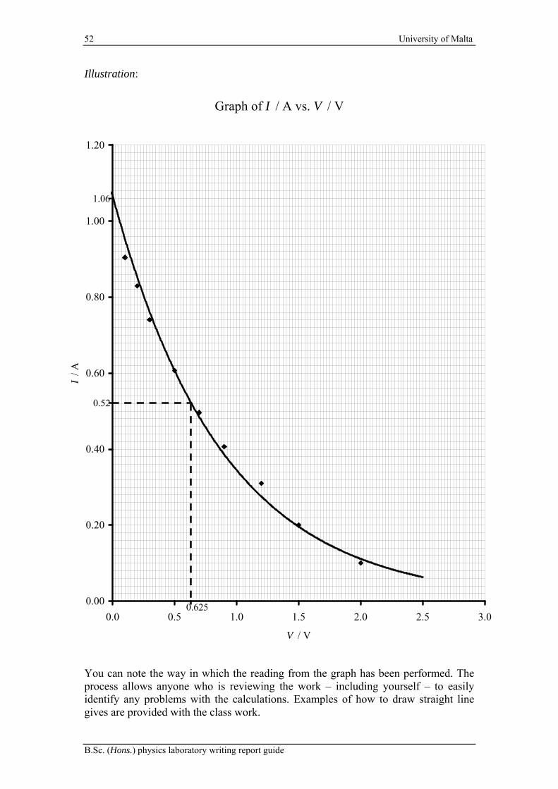
52 University of Malta
B.Sc. (Hons.) physics laboratory writing report guide
Illustration:
You can note the way in which the reading from the graph has been performed. The process allows anyone who is reviewing the work – including yourself – to easily identify any problems with the calculations. Examples of how to draw straight line gives are provided with the class work.
Graph of I / A vs. V / V
0.00
0.20
0.40
0.60
0.80
1.00
1.20
0.0 0.5 1.0 1.5 2.0 2.5 3.0
V / V
I / A
1.06
0.625
0.52

Department of Physics 53
Chapter 3 B.Sc. physics practicals layout
3.8 Calculations
Point 3.8.1:
Calculations should be written down in such a way that a reader can follow through all the steps. For this reason, you should always indicate clearly from where the values are being taken. Example: In the case of values taken from linear regression, say specifically: using linear regression r2 = 0.9235 and m = 2.5 m kg–1.
As a general rule, it is always good practice to make the quantity being determined subject of the formula before you evaluate.
Point 3.8.2:
Indicate units wherever appropriate. With this respect use of negative powers should be preferred. In addition proper formatting of quantities and units is expected.
Point 3.8.3:
In the case that you have an equation you should set it in the straight line form .y mx c Some hints are given below:
- The intercept is a term c that contains only constant variables. This should be the easiest to identity. In the case where there is no constant term, the intercept will be zero.
- In general, the y-term y consists of variables. This should also be easy to identity.
- The last term, mx, is a mixture of constants and variables. It is also the only term left when the intercept and the y-term are identified. The x-term x will then be made up of the variable part, while the gradient term will consist of the constants that are left.
- As an additional help, many a time you will be told what to plot on the x and y -axis. This would immediately provide you these terms leaving only the gradient and the intercept to be determined.
Examples of how to properly write things down and how to go about the procedure have been provided in the class work and the worksheets.
A concern that might arise is which variables should one place on the x-axis and which on the y-axis. In principle, it is easy to rearrange the equation of a straight line so as to set the x-term subject of the formula. To help us with this we have the following convention: The variable/s which we set in the experiment, that are referred to as the independent variable/s are to be placed on the x-axis. Once the independent variables are set, the value of the other variable/s would be automatically determined because of the governing linear equation. These variable/s are referred to as the dependent variable/s since they depend on the ones we have set. The dependent variable/s can be thought of as the variable/s we measure from the experimental setup. For example, when determining the IV-characteristics of an electronic component, we

54 University of Malta
B.Sc. (Hons.) physics laboratory writing report guide
can set the voltage V and measure the current I. In this case, the voltage is the independent variable (as it can take any value we want) and should be plotted on the x-axis while the current is the dependent variable (as its value is fixed once we have set the value of V) and should be plotted on the y-axis.
Point 3.8.4:
Any quantity which you need for the calculations and you have measured should be tabulated in the appropriate section. In this section you should never quote values that have not been tabulated previously or that are not given in the datasheet.
To calculate the gradient and the intercept of the graph you need to use linear regression. The use of a spreadsheet program to help you with the calculations is encouraged. In such cases you should included a printout of the values obtained from the program that contains the values you are going to use in your calculations. The location of the table in your work should be such that it minimizes blank spaces.
Point 3.8.5:
The experiments you are to perform have been widely tested. Hence it is expected that they should provide you with reasonably good estimates of the quantities you are asked to calculate. Should this not be the case you should check your work to make sure it is correct.
The first thing you should do when you check the value is to compare the magnitudes of the experimental and standard values. If you divide the two, their ratio should be between 1 and 4. In this case we say they have the same order of magnitude. If the result can be expressed as 10N then where 1N the we say that the two values defer
by N orders of magnitude. For example if the experimental value obtained for the
acceleration due to gravity is 210 m s then we can say that the result has the same order of magnitude as the standard value. On the other hand, if we obtain 2100 m s then we can say that the values defer by an order of magnitude.
In the case where the values defer by an order of magnitude or more, then you should check the following,
- Any multiplicative factor you have used in plotting the graphs. Possibly you can remove these before you calculate the regression analysis.
- The units are consistent throughout the calculations. This is why it is good practice to include the units with the values so that you can make a homogeneity check.
These are by far the most common reasons for large differences between the experimental determined values and the standard ones.
Note that you do not cheat to make your values equal to the expected values. It is acceptable that in an experiment something can go wrong. If you have followed the procedure correctly and the calculations are correct, you will not be penalised provided you discuss adequately the problem in the last section.

Department of Physics 55
Chapter 3 B.Sc. physics practicals layout
Point 3.8.6:
If you include any comment you should use the passive voice and the past tense.
Once you have finished calculating the values you have been asked for you need to determine the their corresponding uncertainty The calculation of the quantity usually depends on the gradient or the intercept. Thus, it is good to start by determining the standard errors in these quantities (see Section 2.6.3). Once this is done, you can determine the uncertainty using the equations given in Section 2.4.2. Examples have been given in the class work as well as in the worksheets.
Following the determination of the uncertainties, you should also calculate the percentage error and accuracy (see Section 2.5). This will allow you to determine if the experiment was precise and accurate. Note that you need not be asked to calculate these quantities specifically. You are expected to determine them automatically.
3.9 Conclusion or discussion
In general, the conclusion or discussion constitutes a roundup of what has been carried out and what has been achieved. Thus, the first thing you should do is to,
- Summarise what you have done. This should be contained within a sentence or two.
- Provide the values of the quantities you have been asked to determine, including their respective uncertainties.
- Give the accuracy and precision.
Once these have been stated you are expected to comment on the results. Where these accurate and precise? If not, what might have been the reason? This can naturally lead to a discussion of the following,
- The sources of error that most likely have affected your results. - The effectiveness of the precautions taken. - How well the points obtained describe the behaviour expected, which in most
cases is a straight line. - Propose improvements on the procedure adopted. In this case be sensible in
your comments. Remember that in most cases other researchers have extensively studied the setups you have used.
Always remember that you are expected to reasonably explain what might have gone wrong if the experimental result is not of the same order of magnitude as the standard value.
Following this you should answer any additional question that has been set in the worksheets. Most of the time, to do this you will have to make a literature review. By this it is meant that you look up standard textbooks or papers (i.e. articles in peer reviewed journals). This will help you to understand better physical principles involved.
56 University of Malta
B.Sc. (Hons.) physics laboratory writing report guide
Note that while you can use the internet to help you out with the literature review, you should avoid using internet references as these might not be reliable. This subject will be explored in further detail later on.
Finally, even though you are doing a science degree, in this section your linguistic abilities will be tested. Essentially you will be expected,
- Use proper UK English grammar. - Use the passive voice and past tense. - Use an appropriate sentence structure. - Explain your thoughts in such a way that the reader can easily follow your
reasoning. - Develop your argumentation in a logic sequence.
A significant amount of marks for this section depend on your linguistic abilities.
3.10 References
As indicated in the previous section, you are expected to do a literature review revolving about the experiment you have performed. This means you need to look up standard text book or papers to take ideas from them. Hence, you need to acknowledge the source from where you have obtained the information you use. This is done by adequately referencing the source. A detailed explanation of how to carry this out can be found in Section 5.16.
Please keep in mind that adequate referencing in your work is a must. Failure to do so leads to plagiarism that is a very serious academic offence. This will be discussed in detail in Section 5.17.
3.11 Check the sheet to see that you have done everything
Once you have concluded your report it is good practice that you check that everything has been carried out proper. A list of what you should check is given in the next section.

Department of Physics 57
Chapter 3 B.Sc. physics practicals layout
3.12 Check list for B.Sc. practicals:
1. Date
- Write the date of the day when the experiment was performed.
2. Name and Surname
3. Group number (if applicable)
4. Experiment number
5. Aim
- Write a short sentence that indicates what have done.
6. List of apparatus and a diagram
- List all the apparatus.
- Provide a well labelled diagram.
- Use straight lines to assign a label.
- Draw your own diagram, i.e. do not copy and paste it from some source.
7. Procedure
- Repeat what has been done in the method indicating what readings have been taken.
- Make sure that the variables and symbols you will use have been defined.
- Be brief and concise putting without leave anything out.
- Use the passive voice and the past tense.
8. Sources of errors and precautions
- Two subsections sections: Errors and Precautions.
- Use point form, the passive voice and the past tense.
- Be brief and concise as consistent with what you want to say.
- For the errors use relative statements.
- For the precautions write what has been done.
- Write all the errors that you might think about and precautions that you have used in this section.
9. Data collection and tabulation
- Tabulate all the quantities you have been asked to measure.
- Take repeated readings.
- Where appropriate work the uncertainties for the calculated quantities.
- Show all your working.
- Provide appropriate titles for table rows or columns.

58 University of Malta
B.Sc. (Hons.) physics laboratory writing report guide
- Define any symbols you introduce.
- Include the uncertainty for tabulated quantities.
- Values in rows or columns representing the same variable should have the same number of significant figures or decimal places. Where possible they should be consistent with their respective uncertainties.
- Take a minimum of five readings to plot a graph.
10. Graphs
- Plot the graph(s) using a computer program.
- Label each axis using the symbol for the variable together with any multiplicative factor and units.
- Draw the best straight line or curve that can describe all the points.
- Check readings and calculations for points that lie far away from the best straight line or curve. In extreme cases, when the proper pattern is not obtained, you should redo all the readings and calculations.
- Insert Gridlines
- Use greyscale.
- Indicate on the graph any points that are being read.
11. Calculations
- Use clear intelligible steps.
- Indicate units wherever appropriate.
- Set the given equation in a straight line format identifying in the process the intercept, the independent and dependent variables as well as the gradient.
- Make sure that all quantities you are using have been previously tabulated.
- Check if you need to multiply quantities by any multiplicative factors.
- Set quantities you want to evaluate subject of the formula before substituting values.
- Check consistency of units.
- Use linear regression to find the gradient and the intercept.
- Print the results obtained from linear regression (first two columns).
- Do not repeat symbols especially m.
- Make sure that the values obtained are reasonably accurate.
- Be reasonable in the number of decimal place and significant figures with which you quote calculated values.
- Use the passive voice and the past tense for any comment you include.
- Calculate the accuracy wherever possible.
- Calculate the uncertainties for any value you have been asked for.
- Give the uncertainties to one significant figure.

Department of Physics 59
Chapter 3 B.Sc. physics practicals layout
- Determine the percentage error for each of the quantities you have been asked to determine.
12. Conclusion or discussion
- Give a brief description of what has been carried out.
- State the values of the quantities you were asked to determine including the uncertainty, percentage error and accuracy.
- Comment on the results obtained by: Considering any difference in order of magnitude between the
experimental and standard value. Commenting on the percentage error and the accuracy. Comment on the sources of errors giving their relative importance. Discuss the precaution and see if some things could have been performed
better. Commenting on the graph(s) and any associated correlation coefficient. Propose improvements on the procedure adopted.
- Answer any additional question you have been given. Carry out a literature review. Include references wherever appropriate. Do not copy and paste anything from anywhere.
- Show a decent linguistic abilities including: The use of proper UK English, The use of the passive voice and the past tense. The use of an appropriate sentence structure. The proper explanation of your reasoning. The development of argumentations in a logic sequence.
13. References
- Include all reference used.
- Indicate citations in text.
- Do not copy and paste from any source.
14. Check the sheet to see that you have done everything.
- Read the entire worksheet again to see that you have left nothing out.
- Make sure you have answered all questions.
- Make sure that any suggested work has been carried out.


Department of Physics 61
Chapter 4 Errors and Precautions
Chapter 4 Errors and Precautions
Each and every experimental procedure is bound to have an associated error. It is quite unlikely that it will be possible to remove completely the error. However, it will definitely be possible to minimize its effect on the reading to be taken. The following provides a list of the most common sources of error, together with the precautions that should be taken and the way to refer to the error and precaution.
4.1 Alignment
Sometimes the apparatus needs to be aligned in order to obtain reasonable readings. This is especially true in the case of optics experiments. Such an error can be quoted as,
“The apparatus might not have been perfectly aligned.”
Obviously the associated precaution would be that the set up is aligned at its best. This can be written as,
“The apparatus was aligned.”
Note that the error could still be present even though it has been accounted for with a precaution. For this reason it should be mentioned in the error section.
4.2 Cleanliness
Dirt can interfere with the readings being taken, by for example, refracting, diffracting or reflecting incoming light rays or prevent two surface or mediums to make good contact. This error can be referred to as,
“The apparatus might not have been perfectly clean even after cleaning.”
As can be noted from the way in which the error was quoted, it is expected that the apparatus is thoroughly cleaning:
“The apparatus was cleaned.”
4.3 Contact potentials
When two materials are place in contact, electrons will flow from the more electronegative one (which is more prone to give off the electrons) to the other. This creates a potential across the junction, which will either need to be overcome before any current can flow or will add up to the applied potential increasing current flow. Thus, the potential will change across the junction, inducing an error that is simply referred to as:

62 University of Malta
B.Sc. (Hons.) physics laboratory writing report guide
“Contact potentials.”
There is little that can be done for such an inconvenience. One such thing is to reverse the order of the materials in a second junction so that the potential lost at one end would be gained at the other:
“The order of the materials was reversed in successive junctions so as to reduce contact potentials.”
4.4 Human reaction time
The human being is not a perfect machine. For this reason a delay is introduced between the perception of an external stimulus and the reaction to it. This can provide an error when instantaneous reactions are required like for example starting a stopwatch at a particular instant or taking a reading at a pre-established time. This is referred to as,
“Human reaction time.”
There is some debate on whether this error is random or systematic: Take for example the case of measuring the period of oscillation of a pendulum. In general you will start and stop the stopwatch slightly before or after the pendulum is at the position of maximum deflection. The probability of starting the stopwatch before is equal to that of starting the stopwatch after. Thus from this perspective, it would appear that human reaction time is a random error. On the other hand, in order to react to a stimulus, information has to travel from the eyes to our brain where it is processed and then an instruction is sent out to our hands. No matter how fast you think you can be, the average time delay between seeing and acting will never be zero. In fact, on average the human reaction time is around 0.3 s. Hence, from this perspective the human reaction time can be considered to be a systematic error. Effectively the human reflex action contains features of both systematic as well as random errors.
In order to minimise the random nature of this error one should always take repeated readings so that one precaution would be:
“Repeated readings were taken.”
Regarding the systematic bias in the measurement, this can also in some cases be addressed. Suppose you are asked to measure the periodic time of an oscillating system. Then, instead of timing one single cycle for a system, it is possible to measure the time of a number of cycles – usually 20. Subsequently, the total time is divided by the number of cycles to determine the time of one cycle. Since the human reaction time error is only introduce once, when you start and stop the timing, dividing by the number of cycles, will decrease the magnitude of the bias relative to the time of one cycle. Thus the precaution to take would be,
“The time for a number of cycles was determined and then the time for one cycle was calculated.”
Department of Physics 63
Chapter 4 Errors and Precautions
Apart from taking the above precautions it is also necessary to consider the bias introduced when reporting the uncertainty. Thus, no matter how precise your stopwatch maybe, the reported uncertainty in the measurement should never be less than 0.3 s.
4.5 Parallax error
The parallax error is encountered when the measuring device cannot be placed directly in contact with the scale. Examples include analogue meters and measuring a length at a distance due to a limit in the design of the equipment or apparatus. Such errors can be referred to as:
“Parallax error when reading the analogue meter” and “Parallax error when measuring the height of the cantilever from the ground.”
Remember to specify the device if this is not immediately clear.
The precaution for this error involves taken readings from a perspective perpendicular to the measuring device. This act is can be referred to as:
“Readings were taken at eye-level.”
It is to note that in this case no reference needs to be made to the devise as this would have already been specified in the error section.
4.6 Scale rounding-off error
The scale rounding-off error is rarely quoted. It arises when the combined error in a quantity is heavily dependent on that of some term due to the limited precision with which this has been obtained. Using the example indicated in Section 2.2.2, is should be expressed as,
“Scale rounding-off error in the metre ruler: uncertainty 0.001 m .”
In order to decrease this error, it would be necessary to increase the precision of the term causing it. For this reason it is good practice to choose an adequate measuring instrument for each reading. Thus, for example, the device of choice to measure the diameter of a thin wire would be a micrometer screw gauge and not a meter ruler or a venire calliper.
4.7 Scale zero error
Every measuring instrument has a datum or zero level from where to take the readings. This zero level could be off set due to some mechanical or electrical reason. Examples include the shifting of the pointer of a stopwatch from the zero value and the change in the zero reading of a voltmeter due to noise in the circuit. In the first case the error should be referred to as,

64 University of Malta
B.Sc. (Hons.) physics laboratory writing report guide
“The stopwatch had a scale zero error.”
The correction for this error involves noticing the bias of the instrument and adjusting the measurements accordingly:
“The readings were corrected for the scale zero error of the stopwatch.”
The procedure adopted should also be evident in the tabulation of data section, where the shift from zero should be specified. You should then tabulate the values read. Following this you should tabulate the corrected ones. Failure of including this work in the report will lead to a penalization in the markings.
4.8 Variation of dimensions
Frequently the dimensions of an object will vary in space, not simply due to a ware and tear of the object but also to a limit in the production phase. Such an error is frequently encountered when measuring the diameter of a wire (or rod) and can be referred to as,
“Variation of the diameter across the length of the wire (or rod).”
Since this is a random error the way to limit it is by taking repeated readings:
“Repeated readings were taken.”
Note that a good way to account for the variation in diameter of a wire consist of choosing at least five points and at each point take two readings at right angles to each other.
4.9 Calibration
Whenever a measuring instrument is built, there is the need to ensure that for a given input it give the expected output. For example, if we place a 1 g mass on a balance we expect that it indicates exactly 1 g. In order to do this, we need to compare the newly built instrument with some standard, i.e. a quantity or an instrument which has a known uncertainty. If the output from the new instrument is not correct, we need to adjust its inner working so that it gives the proper output.
The process of making sure that a measuring instrument outputs the proper values is called calibration. While ideally, the calibration should be exact, in practice, due to increased costs, it might not be useful to ensure that the precision is excessively high. This gives rise to tolerances (or percentage errors) in the output values that add up to the total uncertainty in the instrument.
The calibration of electronic instruments is of particular importance. The reason for this is that even if these instruments are calibrated when they leave the factory, their calibration tends to shift with time. For this reason, they should be calibrated periodically.

Department of Physics 65
Chapter 4 Errors and Precautions
4.10 List of errors and precautions
The list of all possible errors and precautions is probably too extensive to be summarized in any real effective way. Thus the text below only attempt to summarise the most commonly encountered errors and precautions one expects to come across when doing a simple laboratory experiments. Note that the actual writing down of the error or precaution might need to be adjusted to suite the particular setup you are using. In addition, the comments in square brackets i.e. [] are there only to explain the error and should be omitted during the write up.
4.10.1 Common errors
- System might not have been perfectly aligned. - System might not have been perfectly uniform [this would be due to
imperfection at construction stage]. - Resistive forces have been ignored [for example friction at the point of
pivoting and air resistance on the motion of a pendulum]. - System might not have been perfectly vertical [example a ruler to measure]
or horizontal [example when finding the centre of gravity of a rod]. - Parallax error when reading from instrument [occurs when you are
measuring a scale at a distance, such as length when the metre rule is not in contact with the object or an analogue metre].
- Human reaction time when reading from instrument [occurs due to a human time delay between observation and doing something else such as starting a stopwatch].
- System might not have been perfectly clean [this is particularly important when you are using optical instruments such as lenses, prisms or diffraction gratings].
- Scale zero error in the instrument [occurs when the instrument does not start from zero but from some other value; this is most frequently encountered when using the micrometer screw gauge].
- Variation of dimension along some length [this occurs because rods, bars, wires, disks and the like do not have exactly the same size everywhere due to a limit at the production phase or due to ware and tier].
- Contact potentials [error due to a potential barrier created when wires of two different materials are placed in contact; it applies to most of the experiments involving electric circuits].
- Miscounting a quantity [examples include counting 21 oscillations when you should count only 20]
- Substance not pure [occurs when you want the property of some substance but you are not using a pure sample; an example would be using tap water, which is not pure water].
- Ammeter does not have zero resistance [ammeters should ideally have zero resistance; this cannot be the case in practice as some energy is used to drive them; when using a multimeter as an ammeter its resistance is very small].
- Voltmeter does not have infinite resistance [ammeters should ideally have infinite resistance; this cannot be the case in practice as some energy is used to drive them; when using a multimeter as an voltmeter its resistance is very high].

66 University of Malta
B.Sc. (Hons.) physics laboratory writing report guide
- Instrument might not have been perfectly calibrated. - Resistance of wires was ignored [applies to almost all experiments involving
current]. - Changes in physical properties due to changes in temperature [examples
include wires that heat up causing their resistance to increase; object that heat up and expand; and density of a substance].
- Draught [light flow of air] changing or disturbing the setup [example by cooling some component or pushing a pendulum].
- Mass of hanger was ignored. - Misjudging the position of best alignment when using the instrument
[applies for example when you are using a Vernier scale]. - Apparatus might have moved slightly while doing something [that needs to
be specified] [applies when not every piece of apparatus is held tightly and the change in position affects the results].
- Beam of light was not narrow [in optics experiments this can limit the precision].
- Variation in the supply voltage and/or current [applies to most experiments involving electricity].
- Oscillations might not have been perfectly planar [in the case of pendulum like systems] or linear [in the case of mass spring systems; this is a frequent assumption made in the derivation of the equations].
- Oscillations might not have been sufficiently small [in most derivation oscillation are assumed to have small amplitudes].
- Not enough time might have been given to the system to reach thermal equilibrium.
- The image might not have been perfectly sharp.
Note that the errors have been written in a general form. Whenever they are used in a write-up the terms in curly brackets should be replaced by the instrument, quantity, etc. that it is being referred to. Likewise the terms in square brackets [] should be omitted as these give only some details about the error.
4.10.2 Common precautions
- Repeated readings were taken [since taking repeated readings is considered part of the procedure this type of precaution should be used when no other major precaution has been carried out].
- System was aligned as accurately as possible [see associated error]. - System was as vertical or as horizontal as possible [see associated error]. - Reading on the instrument [to be specified] were taken at eye level [see
parallax error]. - The time for twenty oscillations was found and then divided by twenty to
determine the periodic time [one of the possible precautions corresponding to the human reflex action error].
- System was cleaned [see corresponding error]. - Instrument was checked for scale zero error and if found it was accounted
for [this is done by using the smallest value that the instrument can read as the new zero; see corresponding error].
Department of Physics 67
Chapter 4 Errors and Precautions
- Doors and windows were closed in order to avoid draught [see corresponding error].
- Care was taken not to move the apparatus while doing something [that needs to be specified].
- The instrument [such as micrometer screw gauge and Vernier calliper] was locked in position while taking the readings.
- When using the micrometer screw gauge the ratchets was used to limit the force exerted on the object being measured [avoids squashing the object].
- The system was allowed to stop vibrating before taking the readings. - It was ensured that the connections were tight [applies to almost all
experiments involving electricity]. - The circuit was switched on for the least amount of time possible to take the
readings so as not to heat up the components [applies to most experiments involving electricity; however, sometimes this is not possible].
- Care was taken not to disturb the lamp when lit so as not to damage it [applies only to filament lamps].
- Care was taken not to exceed the scale on the ammeter and/or voltmeter [this could break the instrument whether it is analogue or digital].
- Oscillations were as planar (or linear) as possible [see corresponding error] - Oscillations were as small as possible [see corresponding error]. - The oscillations were timed from a position that was at right angles to the
plane of oscillations at the point where the amplitude is at its maximum [such positioning helps to assess when the system is exactly at its maximum].
- The system was given a significant amount of time to settle before taking readings in order to ensure that it has reached thermal equilibrium.
- Care was taken that the elastic limit of the object was not exceeded.
Note that the precautions have been written in a general form. Whenever they are used in a write-up the terms in curly brackets should be replaced by the instrument, quantity, etc. that it is being referred to. Likewise the terms in square brackets [] should be omitted as these give only some details about the error.

Department of Physics 69
Chapter 5 Write-up formatting
Chapter 5 Write-up formatting
This section details extensive information about how to format a report. The information provided is meant to help you throughout all your undergraduate degree up till your final year. Thus, it contains more details than is required for a practical report. For this reason, you should check with the report example and the notes on the data analysis example worked in class to see what is relevant at this level.
5.1 Importance of proper formatting
It often happens that students are more interested in the scientific content of the write-up then in the actual presentation or formatting. A typical statement that a student may use to justify his attitude is: “If the scientific content of my write-up is good, why should I bother with the formatting?”
However, things are not that easy. Remember that science revolves around having a systematic approach in your dealings. This applies not just to the scientific investigations begin carried out but also to the grammar, punctuation, spelling, formatting and the like involved in the write ups. For this reason, proper formatting of the write-up is part of the skill you are expected to learn while reading your degree.
If such an explanation does not convince you, there is always another way of looking at things. We live in a world that is dictated by aesthetics: When we decide to buy a product, tendentiously we don’t just look at its performance but we also take into consideration it looks. A simple way of checking this out is asking yourself whether you would prefer a car that runs on almost nothing but looks as if it came from prehistoric times or a sports car irrespective of how much it consumes. Put in simple terms: If you want to sell something you’d better make it look nice otherwise you will not make a good profit.
5.2 Language, spelling and grammar
Preferably the write-up should be in UK English, even though US English will also be accepted. However, you should ensure that you don’t mix the two. As a tip, remember that the default spell check language of most word processors is English US. Thus if you want to make sure that you don’t have a mixture of spelling of UK and US English, you should change the default setting.1
The write-up should also be free from spelling and grammatical mistakes. You can use the spell check utility provided by the word processor you are using to help you discover this type of errors. Even so, some typos like writing “meat” instead of “meet” can still persist as it often happens that when we proof read our own work we repeat the same mistakes. One way of trying to reduce the number of spelling
1 Please note that due to the variety of word processors currently in use, it is not possible to give instructions that apply for each one of them. You should refer to the help manual of the word processor you are using for assistance.

70 University of Malta
B.Sc. (Hons.) physics laboratory writing report guide
mistakes is to proof read the work a month or so after first writing it. This will allow you to look at it with fresh eyes.
In some cases sentence structure might be an issue. The generally recommended procedure would be to use short sentences and to limit the number of ideas expressed in one sentence to the minimum. This will avoid getting you into long argumentations that can end up being hard both for you and any reader to follow. As a general rule remember that if a sentence is more than a couple of lines long, it can probably be split up into two. Also a paragraph consisting of one single sentence is definitely not on.
Please remember that it will always be your duty to ensure that the write-up is free from grammatical and spelling mistakes and you should not expect your tutor to deal also with this problem. If you think that your English is not good enough it is permissible to ask a third person to proof read your work. This does not mean that you are allowed to ask a third person to write the report himself but just to read your work and suggest improvement. Obviously the person’s work should be duly acknowledged in your write-up.
5.3 Font and font size
The font should be preferably Times New Roman. This will avoid confusion between similar letters and numbers such as the letter “l” (ell) and the number “1” (one).
Regarding the font size this should be set to 12 points so as to make the text readable.
5.4 Paragraph and line formatting
There are two accepted ways of formatting a paragraph:
- Either you start flush form the left and you skip a line between paragraphs, or
- You indent the first line but then you don’t skip a line between paragraphs.
You may choose any of the two. However, a mixture of the two, like indenting the first line and then skipping a line each time, is not acceptable.
The paragraph should have a margin to the left and to the right of about 3 cm. In addition a space of about 2.5 cm should be left at the top and bottom of the page. The typed text should also be justified.
Regarding the line spacing in general this should be kept to 1.5. Note that the default value in the most common word processors is single spacing (i.e. 1).

Department of Physics 71
Chapter 5 Write-up formatting
5.5 Capitalisation
Well this might sound easy – just ensure that the first letter at the beginning of each sentence and of names is a capital letter. In most cases you are right. However, you should remember that capital letters are generally harder to read than small captions. Thus you should try to limit the amount of capital letter you use. For example a title consisting of more than one word should only have the first one capitalised unless a name is used. Likewise if you want to emphasise some word or words, you should try to use italic, bold or underline rather than capitalise. This will make your work more readable.
5.6 Footnotes
Footnotes are a way of inserting annotations to the main text. They should be used with care so as not to break the flow of the work. In the case a footnote is required this should be placed at the bottom of the page. The preferred symbols to use in order to cross-refer to the footnote are Arabic numerals superscript, with the footnotes being numbered consecutively according to the order in which they are referred to in the main text. Preferably numbering should restart on every page.
The footnotes should be written in the same font as the main text but with a smaller font size, namely 10 points. They should also be justified and the order in which they are listed should reflect the order in which they are cross-referred to in the main text.
5.7 Short hand notations and acronyms
You should not assume that the reader is familiar with short hand notations or acronyms even if they are standard in the field of work. Thus you should define all short hand notations and acronyms the first time you use them. In the case the number of short hand notations and acronyms is extensive, you should write a list explaining them at the beginning of your work.
5.8 Numerical values
In the case numerical values appear in the text, it is customary to write numbers from zero to ten as words while higher order values using Arabic numerals, namely a combination of 0, 1, 2, 3, 4, 5, 6, 7, 8 and 9. In the case of a list containing values higher and lower than 10 they should all be written using Arabic numerals. On the other hand, if the number occurs at the beginning of a sentence this should be written as text.
It is important to keep in mind that the Arabic numerals should never be italic not even when they are used as subscripts.
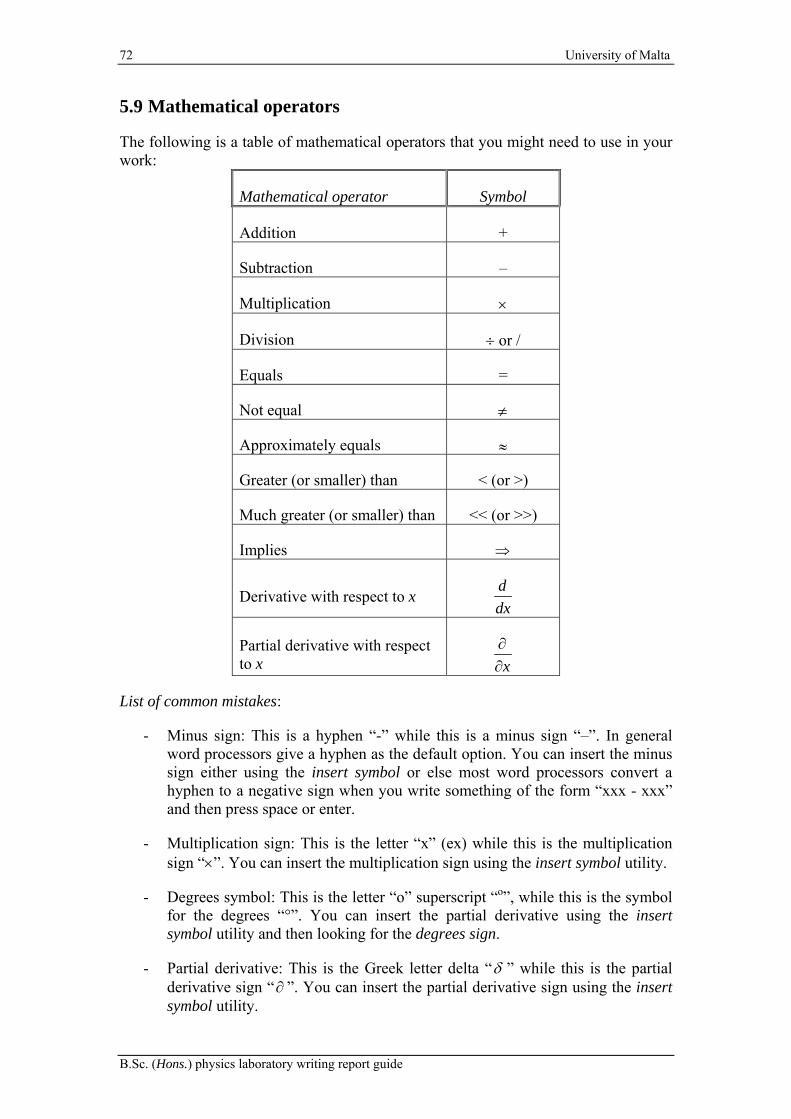
72 University of Malta
B.Sc. (Hons.) physics laboratory writing report guide
5.9 Mathematical operators
The following is a table of mathematical operators that you might need to use in your work:
Mathematical operator Symbol
Addition +
Subtraction –
Multiplication
Division or /
Equals =
Not equal
Approximately equals
Greater (or smaller) than < (or >)
Much greater (or smaller) than << (or >>)
Implies
Derivative with respect to x d
dx
Partial derivative with respect to x x
List of common mistakes:
- Minus sign: This is a hyphen “-” while this is a minus sign “–”. In general word processors give a hyphen as the default option. You can insert the minus sign either using the insert symbol or else most word processors convert a hyphen to a negative sign when you write something of the form “xxx - xxx” and then press space or enter.
- Multiplication sign: This is the letter “x” (ex) while this is the multiplication sign “”. You can insert the multiplication sign using the insert symbol utility.
- Degrees symbol: This is the letter “o” superscript “o”, while this is the symbol for the degrees “°”. You can insert the partial derivative using the insert symbol utility and then looking for the degrees sign.
- Partial derivative: This is the Greek letter delta “ ” while this is the partial derivative sign “ ”. You can insert the partial derivative sign using the insert symbol utility.

Department of Physics 73
Chapter 5 Write-up formatting
- Delta operator: When the capital Greek letter “Δ ” is used as an operator it is not italic. Examples include its use for the gradient and uncertainties.
5.10 Brackets
It can often happen that you will have to use a set of brackets within another set of brackets. In order to facilitate the understanding of the order of the brackets the following system is suggested:
- First use a round bracket, i.e.
- Then use a square bracket, i.e. - Finally use a curly bracket, i.e. - If this is not enough, repeat.
Thus you should have something of the form .
5.11 Units
In general the units should be in SI unless one is dealing with some particular subject where there is some other conventionally employed system. They can be written either in full for example newton seconds or else using the standard abbreviations for example N s. However, a mixture of the two would not be considered acceptable.
There should be a space between the numerical value and the unit and another between each unit. The latter requirement is needed to distinguish between for example metres seconds (m s) and milliseconds (ms). The negative power notation like 1m s is preferred to the slash notation like m/s.
It is important to keep in mind that the standard abbreviations of units should never be italic.
Common mistake: The fact that a space should be included between the unit and the value includes the use of percentages (%) and degrees Celsius (°C). The only common expectation to this rule is given by the degrees (°) when they refer to angles, in which case no space should be included.
5.12 Variables
The way in which we write variables depends on what they represent. In the case they represent quantities that have only a magnitude, we can write them in italic like for example the speed which can be written as v. It is also generally accepted to write symbols representing matrices and tensors in the same way.
If the quantity being represented is a vector the symbol should either be bold, e.g. v or over lined with an arrow, e.g. .v

74 University of Malta
B.Sc. (Hons.) physics laboratory writing report guide
Note that letters indicating a point are not considered as variables and hence should not be written in any special way. Thus for example if we have two points we can call them Points P and Q and the displacement between them can be written as PQ.
In the case the number of symbols used in the work is very large, it would be recommended to have a list of symbols at the beginning of the work. The list should start with Roman type followed by the list of Greek symbols each of which should be given in alphabetical order.
5.13 Subscripts and superscripts
The way in which subscripts and superscripts are written follows the same rules as those given for numerical values and variables. Thus, Arabic numeric used as subscripts and superscripts should not be italic while variables should generally be italic unless they represent vectors, in which case we can write them as bold. Examples include, 2 ,x iy and .dv
In the case the subscript or the superscript is a word, this should not be italic. For example the effective velocity can be written as, Effective.v If one wants to abbreviate
effective to “Eff” it is possible to write Eff .v In short if the subscript or superscript
represents a word or a short hand for a word it should not be italic.
As a particular point, please note that generally the original or initial value is denoted by a zero as a subscript not the letter “o” (ow). Thus the original length should be written as 0.l
In the case that the number of subscripts and superscripts used is extensive, it is recommended that a list is provided at the beginning of the work. This should be placed immediately following the list of variables (Section 5.12) with the roman type coming first, and the Greek symbols second.
5.14 Equations
For long reports, dissertations and papers, equations should be labelled using consecutive Arabic numerals, starting from one, in the same order in which they appear. Conventionally the number is placed in parentheses (i.e. round brackets) flash on the right hand side of the paper as shown below:
2
2
2exp
2
1
x
xf (10)
If the work is extensive and there are many chapters, it is good practice to include the chapter number at the beginning. For example if the equation above is the 10th in chapter two it can be labelled (2.10). If this notation is used then the equations should start to be numbered again from one at the beginning of each chapter.

Department of Physics 75
Chapter 5 Write-up formatting
Regarding the location of the equation, this can either be placed at the centre of the remaining space or else it can be written after an indentation to the left. Both of them will be allowed provided the work is consistent.
In the case you are wondering how you can write the above easily using a word processor, the suggestion would be to use tables. As a tip also remember that most word processors offer the possibility of automatically numbering your equations.
The numbering of the equations allows easy reference to them. For example to refer to the equation above, it is possible to write Equation 10, Equation (10), Eq. 10 , Eq. (10) or simply (10). All of them would be acceptable provided the work is consistent. The only limitation occurs if you refer to the equation at the beginning of the sentence, in which case you should write the word “Equation” in full.
5.15 Figures and tables
Figures and tables should be used to represent results or to help in explaining things. They should be used with caution as too many figures or tables might hinder the reader from following the arguments in the text. If the number of figures or tables becomes extensive, and no way is found in order to limit their number, it is possible to place them in an appendix and only include in the main text a summary of what they represent.
The figures and tables should have a caption explaining what is contained within them. In general the caption should start with the words Figure for a figure and Table for a table followed by a number. Both the letter and the number should be written bold. The number is assigned in increasing order starting from one depending on their appearance in the work. Thus the first figure to appear is assigned the number one, the second one to appear the number two and so on. In the case the work is very long and there are a number of chapters, it is customary to also label the figures and table using the chapter number in which they are included. In this case the numbering restarts at every chapter.
All figures and tables that are included in the work should be referred to in the main text. One should take care that if a figure or a table is referred to in the main text, it should also be found somewhere in the work. The order in which the tables or figures are referred to should also reflect their position within the text. Thus, for example, the first figure to appear in the text should be labelled Figure 1 and should also be the first one to be discussed in the main text.
In order to refer to the figures and tables in the main text one can use the label and the number. Thus if you want to refer to the second figure you can just write Figure 2 or Fig. 2. In the latter case the full label (Figure or Table) should be used when the cross reference appears at the beginning of a sentence. While there are other ways of referring to the figure and the tables, such as the use of the words, “above” or “below” their use is discouraged. The reason for this is that the position of the figure or table might change in time due to formatting needs so that something that was initially above might end up below leading to an error in the cross-reference. Hence, in order to avoid such problems, it is advisable to use only the caption and the number.
76 University of Malta
B.Sc. (Hons.) physics laboratory writing report guide
Please note that to improve the flow of the work the figures and tables should be blended within the text so as to maximise the use of the available space. Preferably their location should be close to the location in the text where they are referred to.
A list of figures and another one of tables should be provided at the beginning of the work irrespective of how many figures or tables have been used.
5.16 References and bibliography
Applying proper references is a factor of major importance in any scientific write up. References are used either to validate the arguments or concepts being expressed or else to acknowledge the fact that what is being written is not a product of one’s own work but of someone else’s. One should be very careful on how to deal with references as mismanagement can lead to plagiarism which is a type of academic misconduct that is considered to be very series and can lead to disciplinary actions against the perpetrator.
The use of references has two parts. One of them is to have a section at the end of the work, before the appendices, where you include a full description from where you have obtained the reference. The other is to cross-refer to the reference in the main text whenever you want to validate your argumentations or indicate that you are using someone else’s work. The details of how to do this depend on which referencing system you decide to adopt. The main referencing systems are the Harvard and the Vancouver (or author-number) system. These are described in the sections that follow.
On going through these sections, please keep in mind that different institutions can adopt slight variations to what is suggested in this work. All of these will be considered acceptable in your write-ups provided you are consistent throughout your work.
Note that all the references included in the reference section should be cross-referred to in the main text. In the case that you have read a book, an article or the like but you are not using anything directly in the main text, then you should include that reference in another section called bibliography. Thus the bibliography will contain all the sources you came across in you work and that you actually have read but that you are not making direct use of them in your work. For consistency the style used in your bibliography should be the same one employed in the reference section. Note that a bibliographic section might not be needed if all references are used in the main text.
5.16.1 The Harvard system
Reference section:
The way in which the references are described in this section depends on the nature of the source. Thus for example the way to write a reference of a book will be different from that of a paper from a journal. A comprehensive list of the format that should be adopted when writing references is given below. Once the reference has been written in the appropriate manner, the list should be arranged in alphabetical order.
Department of Physics 77
Chapter 5 Write-up formatting
Books:
Surname, Initials (Date of publication). Name of book in italic; Publication House: Country of publication.
Illustration:
Batschelet E. (1981). Circular Statistics in Biology; Academic Press: New York.
Papers:
Surname, Initials (Date of publication). Title of paper; Title of Journal in italic, volume(issue) in bold, pages.
Illustration:
Ackermann, G.R. (1983). Means and Standard Deviation of horizontal wind components, Journal of Applied Meteorology, 22(2), 959–961.
Castans, M. and Barquero, C.G. (1998). Some Comment on the Study of Low Persistence Wind: Discussion, Atmospheric Environment, 32, 253–256.
Technical report:
Sometimes, a commercial company, a state agency or some academic institution produce a report that is not properly published. By this it is meant that the work carried out as well as conclusions are not published in a book or a peer reviewed journal. Hence such technical reports, as they are called, are considered to be non-standard references (cf. Section 5.16.4). At the same time, given that they are endorsed by the commissioning entity and are written by fully qualified people, the contents can in general be taken to be correct. However, alternative sources, namely books or/and published journal articles, detailing the same material should be preferred over technical reports. In case this is not possible, you can use the following format in order to list them in the reference section,
Surname, Initials (in case of a single or multiple authors) or corporation name (in case of a corporation), (Date of publication). Title of technical report in italic, report reference number or code if available; institution endorsing the report, url address if available online, date of last accessed if available online.
Illustration:
Cho, S., Im, P. and Haberl, J.S. (2005). Literature Review of Displacement Ventilation, Technical Reports from the Energy Systems Laboratory.
PG&E (1997). Thermal Energy Storage Strategies for Commercial HVAC Systems, an application note of the Pacific Gas and Electric Company, available online at http://www.pge.com/includes/docs/pdfs/about/edusafety/training/pec/inforesource/thrmstor.pdf, last accessed on 3rd March 2012.

78 University of Malta
B.Sc. (Hons.) physics laboratory writing report guide
Websites:
Websites are a type of non-standard reference. Thus caution should be used if one decides to resort to them (cf. Section 5.16.4). Given that it is only recently that references to websites have become popular, the way in which they are referred to is in constant evolution. The following describes one of the currently suggested versions:
Surname, Initials (in case of a single or multiple authors) or corporation name (in case of a corporation), (Date of publication), title of page in italic, url, date on which it was last accessed.
Illustration:
Weisstein, E.W. (2010). Exponential Function From MathWorld--A Wolfram Web Resource, http://mathworld.wolfram.com/ExponentialFunction.html. Date accessed, 14th of August 2010.
Busuttil C., (2009). timesofmalta.com – What’s that mysterious light in the night sky?, http://www.timesofmalta.com/articles/view/20090323/local/whats-that-mysterious-light-in-the-night-sky, Date accessed, 14th August 2010.
The data of access is required due to the volatile nature of the websites that can change daily without prior notice.
Citations in text:
In order to support your argumentations or in order to indicate that the work you are referring to has not been conducted by yourself, a cross-reference is included immediately after or before the text under consideration. For all the case mentioned above, if the number of authors is less than three the format (Surname, Date) or Surname (Date) is used. Example (Johns, 1986) or Johns (1986), (Johns and Smith, 1986) or Johns and Smith (1986), Johns and Smith (1986) and Walters (1995) or (Johns and Smith, 1986, Walters, 1995). If the work has been carried out by more than two authors than you can use the format Smith et al. (1990) or (Smith et al. 1990).
Sometimes accessing the original text where work was originally carried out can be difficult and we only get to know the information we need through a second source, called the secondary source. In such a case we need to make clear that we did not read the primary source. This can be carried out by using one of these formats: Jones (1986) as cited by Smith (1990); Jones (1986 cited in Smith, 1990); or (Jones, 1986 cited in Smith, 1990).
5.16.2 The Vancouver system
Reference section:
The reference section is very similar to the one for the Harvard system except that each reference is given a number. The order of the reference should reflect the order in which the references appear in the text. Thus, the first reference to appear in the

Department of Physics 79
Chapter 5 Write-up formatting
text should be given the number one, the second reference to appear the number two and so on.
Illustration for a book:
[1] Batschelet E. (1981). Circular Statistics in Biology; Academic Press: New York.
Illustration for a paper:
[2] Ackermann, G.R. (1983). Means and Standard Deviation of horizontal wind components, Journal of Applied Meteorology, 22, 959–961.
[3] Castans, M and Barquero, C. G. (1998). Some Comment on the Study of Low Persistence Wind: Discussion, Atmospheric Environment, 32, 253–256.
Illustration for a technical report:
[4] Cho, S., Im, P. and Haberl, J.S. (2005). Literature Review of Displacement Ventilation, Technical Reports from the Energy Systems Laboratory.
[5] PG&E (1997). Thermal Energy Storage Strategies for Commercial HVAC Systems, an application note of the Pacific Gas and Electric Company, available online at http://www.pge.com/includes/docs/pdfs/about/edusafety/training/pec/inforesource/thrmstor.pdf, last accessed on 3rd March 2012.
Illustration for a website:
[6] Weisstein, E.W. (2010). Exponential Function From MathWorld--A Wolfram Web Resource, http://mathworld.wolfram.com/ExponentialFunction.html. Date accessed, 14th of August 2010.
[7] Busuttil C., (2009). timesofmalta.com – What’s that mysterious light in the night sky?, http://www.timesofmalta.com/articles/view/20090323/local/whats-that-mysterious-light-in-the-night-sky, Date accessed, 14th August 2010.
Citations in text:
In the text, it is possible to refer to the references using their corresponding number. For example if you want to refer to the fifth reference you just need to write [5]. In the case you want to refer to a number of references in succession, for example from one to four, you can use [1-4]. You can also combine single and continuous referencing such as [1-3,5] meaning that you are referring to reference one to three and five. Regarding information obtained from secondary sources one of the following formats can be used, [1] as cited by [2] or [1] (as cited by [2]).
An alternative that is commonly used is to include the name of the author. In the case where there is only one author it is possible to write Johns [1]. If two authors are involved one can write Johns and Smith [2] and while Johns et al. [3] can be adopted

80 University of Malta
B.Sc. (Hons.) physics laboratory writing report guide
in the case of three or more authors are involved. Note that the references are sometimes written as superscripts.
Please remember that the order of the references in the reference section should be the same as that in the main text. Thus the first reference to use is [1] and not for example [3].
5.16.3 Comparison of the Harvard and Vancouver systems
The Harvard and Vancouver systems are widely used with one beginning preferred in journals on some topic and the other being preferred in journals with a different topic. Thus you are free to use whichever you prefer.
However, there are some points to consider when carrying out the choice. In the Harvard system, you can include a new reference in the middle of the others without major modifications of the text. On the other hand if you include a new reference in the Vancouver system, you will have to renumber all the following references both in the reference section as well as in the text. The Harvard system has the added advantage that if you refer to a well known source in your field, for example Batschelet (1981), from the name and year one can easily identify the work without having to check the reference section.
The advantage of the Vancouver system over the Harvard system is that you can condense a lot of references. The fact that you can identify multiple consecutive references by simply writing for example [10-25] dramatically reduces the amount of text needed.
5.16.4 Non-standard references
Non-standard references refer to work that has not been formally published and hence has not been peer reviewed. The fact that it has not been validated makes its use questionable. For this reason efforts should be taken to try to avoid their use and instead adopt standard references such as books and journal articles.
The most common of the non-standard references are websites. In this internet era it has become common practice to first browse the internet for information before looking somewhere else. However, in doing so, one must always remember that there is nothing that regulates the information found on websites. Thus you need to use the information with caution.
Case in point is Wikipedia – possibly the currently number one source of information on the internet and usually the first one to pop up when queering a search engine. While Wikipedia gives very useful information, there is nothing to guarantee that what is written is exact. Wikipedia can be edited by anyone, anytime, without any quality control. Thus, one cannot trust blindly what is found on it.
So should one just forget about Wikipedia? Not necessarily. Wikipedia generally provides an extensive list of peer reviewed sources. In this way Wikipedia can become a very useful starting point for obtaining peer reviewed information. This

Department of Physics 81
Chapter 5 Write-up formatting
means that you are allowed to use Wikipedia as one of your references, however it should never, ever be your main or sole reference on the topic.
5.16.5 When do I need a reference?
If you are not sure if you need a reference or not ask the following two simple questions:
- Did I know the subject before reading about it?
- Did “I borrow” any idea or words?
If the answer to the first one is no or the answer to the second one is yes, you need a reference. This is especially true of the second one, where it is likely that you are plagiarising some work. In this case you might need to do more than just adding a reference. One example would be to write the “borrowed” words between inverted commas to indicate that those are not your own words but those of the author or authors indicated in the reference.
5.17 Plagiarism and collusion
Plagiarism and collusion two similar unethical academic behaviour. However, they are not strictly the same thing. The former refers to inappropriate copying of some else’s work, namely because the original authors are not fully acknowledged. Another way to say it is to induce someone to think that you have done the work when in reality you just copied it in some way.
On the other hand collusion occurs when student work together and present their common efforts as two distinct works. This is a naturally occurring problem when students are asked to work in groups. However, at undergraduate level and beyond, students are expected to write reports on their own even if some practical part has been accomplished in collaboration with someone else. Whenever there is some collaborative work, only the values measured should be the same. The remainder, including
- the tabulation and formatting of the data,
- graphs, and
- the calculations of values and uncertainties
is expected to be different.
Both plagiarism and collusion are considered to be very serious academic offense and severe disciplinary actions can result. To help you understand the what exactly constitutes plagiarism the University of Malta provides Plagiarism and collusion guidelines that are downloadable from http://www.um.edu.mt/__data/assets/pdf_file/0009/95571/University-Guidelines-on-Plagiarism.pdf as well as the manual How to avoid plagiarism found at http://www.um.edu.mt/__data/assets/pdf_file/0006/95568/how-to-avoid-

82 University of Malta
B.Sc. (Hons.) physics laboratory writing report guide
plagiarism.pdf. Furthermore, students following an undergraduate degree at the University of Malta are expected to follow the course LIN1063 Academic Reading and Writing in English (http://www.um.edu.mt/linguistics/studyunit/LIN1063) where the subject is treated at length.
A simple way of avoiding plagiarism is not to copy and paste any material from any source. If you cannot avoid copying the material, then you should ensure that any material that has been copied is adequately references so as to make it clear it is not your work but that of the others. In the case you copied whole phrases or paragraphs, as discussed above, these should be placed between inverted comas and add a referenced. As for tables and figures, you should include “copied from” before the reference in the case you have copied them. In the case of figures, if you draw the figure from scratch but do not change it appreciable, then you should include “adapted from” before the reference. The “copied from” and “adapted from” together with the reference should go in the caption. Note that in principle, you should ask for permission from the copyright owners before you can copy a table or a figure. Hence you should try to draw your own figures wherever possible.
To help you identifying any problem with your work, you will be asked to upload the final document on a Turnitin portal that will be available on the Virtual Learning Environment (VLE). There will be two such portals, the first where you can upload a draft of the work and the second to upload the final version of the work. The draft Turnitin portal is provided so that you can check for plagiarism problems. You can then correct these without incurring any penalisation and upload the updated version in the final Turnitin portal. Note that you are only allowed submit your work only once to the draft assignment Turnitin portal.
Interpreting the result of the Turnitin portal might not be straight forward. To help you with this consider the situation where you find a sentence marked as shown below.
The Turnitin portal is telling you that the sentence is copied from the Source 3 (that you will find on the right hand side.). Such instances should be avoided. The sentence should be rephrased in your own works.
A more complicated instances occurs when you have various marking in the same paragraph that appear to originate from the same source as shown below.
This is an example of what should be avoid. If you encounter a situationwhere there is a sentence that is marked in the same way as this one, then youcan be sure that you have a problem of plagiarism. Avoid such instances.
3
Department of Physics 83
Chapter 5 Write-up formatting
This is indicative of a type of plagiarism called patch writing. This occurs when one or more phrases have been copied from some source and then some words have been changed here and there. Such instances are still considered to be plagiarism and should be avoided by rewriting the whole structure. More information about Turnitin and how to use it can be found at http://www.um.edu.mt/vle/pds/students/pdstraining. If in doubt on how to interpret the result, ask the demonstrators, coordinators, or tutor to help you out. However, remember that the onus of ensuring that your work is not plagiarised lies only with yourself and with nobody else.
The Turnitin portal will not help you to check instances of collusion as these will only be highlighted in the final assignment Turnitin portal when cross comparison between the submissions takes place. The best way to avoid collusion is to work on your own. This will ensure that you cannot copy from someone else who is working on the same project. Furthermore, no one else can copy from you.
This is another example of what should be avoid. At time it would appear thatyou do not have a single sentence originating from the same source. However,different parts of a paragraph have been marked to originate from the samesource. This is known as path writing and is still a type of plagiarism. It iscalled path writing and occurs when you copy a paragraph from some sourceand simply change a couple of words here and. Once gain such instancesshould be avoided.
3
3
3
3
3


Department of Physics 85
Chapter 6 Instrumentation
Chapter 6 Write-up formatting
6.1 The spectrometer
A spectrometer, or more precisely an optical spectrometer, is an optical instrument that can be used to investigate various properties of light such as its deflection due to reflection, refraction or diffraction as well as its polarization. A schematic illustration of all its most basic features is shown in Figure 6.1.
Figure 6.1 Schematic illustration of the basic components of a typical spectrometer.
As can be observed, a spectrometer is made up of a significant number of components. Some of them are used to focus the collimator and the telescope such as the focus knobs while others keep the part in position and allow for fine adjustment. The way how to use them will shortly follow. However, before discuss how to set up the spectrometer, it is worth giving a brief description of how this instrument works.
6.1.1 Mode of operation of the spectrometer
A spectrometer is an instrument devised to investigate what happens to a parallel beam of light when it passes through an optical devise. Its simplest configuration, when there is no optical devise on the turntable and the telescope is aligned with the collimator, is illustrated schematically in Figure 6.2.

86 University of Malta
B.Sc. (Hons.) physics laboratory writing report guide
Figure 6.2 Top view of the path light takes through a spectrometer.
Light from some source enters the system through the slit in the slit plate at the far end of the collimator. The slit is place on the focal point of the collimator’s lens. Thus the light from the slit is converged into a parallel beam before it exits the collimator. This is then focused again by the lens in the telescope. Past the focal point, the expanding beam is converted back to a parallel beam by the lens in the eyepiece.
In such a configuration the need for an eyepiece might not be immediately obvious. Its necessity arises because the eye itself is an optical instrument. As a result, it would not be able to view the real image produced by the telescope’s lens at the focal point (Figure 6.3). For this reason, a virtual image is produced by the eyepiece’s lens that can be then focused on the retina by the eye’s lens.
Figure 6.3 The detailed view of the use of an eyepiece in a spectrometer.
This setup is actually not enough. If the experimenter just looks into the eyepiece the field of view would be too large, making it difficult to decide what to look at. For this reason cross-wires (or cross-hairs) are introduced at the focal point of the telescope’s lens so that the experimenter can concentrate on them.
All the optical parts mentioned so far require adjustment before accurate readings can be taken. For example the slit must be at the focal point of the collimator’s lens while the cross-wire on that of the lenses of the eyepiece and the telescope. This requires a number of adjustments before any measurement can be made. These will be discussed in the next section.
Slit plate
SourceTelescope
Eyepiece
Turntable
Lens of theeyepieceCollimator
Lens of the collimator
Lens of the telescope
Telescope
Lens of thetelescope Cross-wires
Eyepiece
EyeImage formingon the retina
Lens of theeyepiece
Image formed by the telescope lenson the cross-wires
Parallel beam of lightfrom a distant object
Lens of The eye

Department of Physics 87
Chapter 6 Instrumentation
6.1.2 General focusing the spectrometer
The components that need to be adjusted in order to focus the spectrometer are the eyepiece, the telescope, the collimator and the slit plate. There are various ways in which this can be done, with the most advanced of which being Schuster’s method. However, here a simpler method is adopted:
Step 1: Focusing the eyepiece
Look at the cross-wires through the eyepiece. Then push the eyepiece inwards or outwards until the cross-wires are clearly visible.
Step 2: Focusing telescope
The telescope needs to be focused at infinity. A simple way of doing this is to focus the instrument on something which is at a very large distance. The suggested way of doing this is to place the telescope on a stool in the main hall and then obtain a clear image of the chemistry building. Focusing of the telescope on the distant object can be achieved by rotating the moving telescope focus knob (see Figure 6.1) clockwise or anticlockwise as necessary. Care must be taken not to rotate the knob too much as this may force it beyond its limits and damage the tread. Note the image of the distant object must be overlaid on the cross-wires since these are found on the focal point of the telescope’s lens (see Figure 6.3).
Step 3: Focusing the collimator
Once the telescope and the eyepiece are focused it is easy to focus the collimator. First make sure that the slit palate is at least slightly open. Then place it in front of the light source. At this point align the moving telescope with the collimator and look at the slit through the eyepiece as indicated in Figure 6.2. The focus knob on the collimator (see Figure 6.1) can now be rotated clockwise or anticlockwise until a clear image of the slit is visible.
Step 4: Adjusting the slit
The beam of light needs to be as thin as possible, meaning that the slit should be as small as possible. At the same time it should be sufficiently bright to allow for the reading to be easily taken, which would require the slit to be wide. Hence a trade-off needs to be taken between the two requirements.
In order to make the required adjustment, look at the slit through the eyepiece. Then turn the slit width adjust screw (see Figure 6.3) clockwise or anticlockwise until the beam is about 1 mm thick. This should give a good trade-off between width and luminosity.
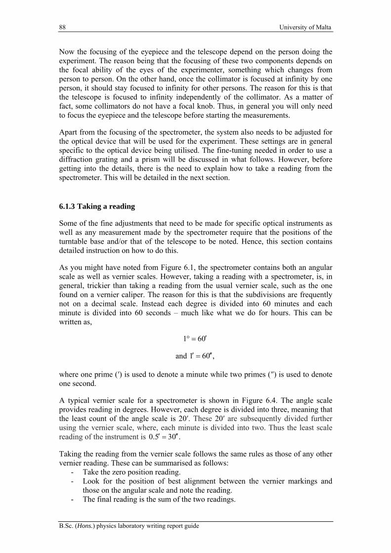
88 University of Malta
B.Sc. (Hons.) physics laboratory writing report guide
Now the focusing of the eyepiece and the telescope depend on the person doing the experiment. The reason being that the focusing of these two components depends on the focal ability of the eyes of the experimenter, something which changes from person to person. On the other hand, once the collimator is focused at infinity by one person, it should stay focused to infinity for other persons. The reason for this is that the telescope is focused to infinity independently of the collimator. As a matter of fact, some collimators do not have a focal knob. Thus, in general you will only need to focus the eyepiece and the telescope before starting the measurements.
Apart from the focusing of the spectrometer, the system also needs to be adjusted for the optical device that will be used for the experiment. These settings are in general specific to the optical device being utilised. The fine-tuning needed in order to use a diffraction grating and a prism will be discussed in what follows. However, before getting into the details, there is the need to explain how to take a reading from the spectrometer. This will be detailed in the next section.
6.1.3 Taking a reading
Some of the fine adjustments that need to be made for specific optical instruments as well as any measurement made by the spectrometer require that the positions of the turntable base and/or that of the telescope to be noted. Hence, this section contains detailed instruction on how to do this.
As you might have noted from Figure 6.1, the spectrometer contains both an angular scale as well as vernier scales. However, taking a reading with a spectrometer, is, in general, trickier than taking a reading from the usual vernier scale, such as the one found on a vernier caliper. The reason for this is that the subdivisions are frequently not on a decimal scale. Instead each degree is divided into 60 minutes and each minute is divided into 60 seconds – much like what we do for hours. This can be written as,
1 60
and 1 60 ,
where one prime (′) is used to denote a minute while two primes (″) is used to denote one second.
A typical vernier scale for a spectrometer is shown in Figure 6.4. The angle scale provides reading in degrees. However, each degree is divided into three, meaning that the least count of the angle scale is 20′. These 20′ are subsequently divided further using the vernier scale, where, each minute is divided into two. Thus the least scale reading of the instrument is 0.5 30 .
Taking the reading from the vernier scale follows the same rules as those of any other vernier reading. These can be summarised as follows:
- Take the zero position reading. - Look for the position of best alignment between the vernier markings and
those on the angular scale and note the reading. - The final reading is the sum of the two readings.

Department of Physics 89
Chapter 6 Instrumentation
Figure 6.4 Schematic illustration of a typical vernier scale of a spectrometer.
To illustrate the method, we will use Figure 6.4: - From this it can be noted that the zero position which is located on the vernier
indicates that the reading is between 149 and 149 20 . Thus we take 149 ,i.e. the least value, and see how much we need to add to this.
- The second reading is taken from the vernier by looking at the position of best alignment. By this it is meant the position at which one of the lines on the vernier scale is aligned exactly with one of the lines of the angle scale. In the case of Figure 6.4 this occurs at 9.5 . This part can be particularly difficult to assess as a number of lines might appear to be aligned. A useful trick in these cases is to look for the first position starting from the left where the lines are almost aligned. Then repeat, this time starting from the right. It would then follow that the line you are looking for is somewhere in-between.
- Finally we need to add the two values i.e. 149 and 9.5 . The final result is thus, 149 9.5 0.5 . (Note the inclusion of the uncertainty.) A simple check for this value is given by the fact that the final value is in the range identified in the first step above.
Note that a typical spectrometer has two vernier scales for the turntable base and another two for the rotating telescope. Each pair of vernier scales is at 180 to each other. These are used to obtain concurrent repeated readings.
Before proceeding to the next section it is worth remarking that the scale shown in Figure 6.4 is very small, making it difficult to read with the naked eyes. For this reason, it is usually read with the help of a lens.
6.1.4 Using a diffraction grating
In order to use a diffraction grating with a spectrometer we need to ensure that: - The grating is perpendicular to the direction of the beam. - The slits in the grating are along the vertical direction of the beam.
Before proceeding to discuss the steps needed to make these settings you should make sure that you know how to take a reading from the vernier scales (see Section 6.1.3)
10
Zero position at 149°
Position of best alignment at 9.5′
Vernier scale
Angles scale

90 University of Malta
B.Sc. (Hons.) physics laboratory writing report guide
and be familiar with the components of the spectrometer (see Figure 6.1). In particular you should note that the turntable has three adjustable levelling screws that can be accessed from below. These will be used to level the turntable such that the second criterial above is met.
The steps you need to follow in order to setup the spectrometer with the diffraction grating are as follows:
1. Make sure that the turntable is clear so that the path of the beam is unobstructed.
2. Align the telescope with the collimator (Figure 6.5(a)) and position the beam such that it is at the centre of the cross-wires (Figure 6.5(b)). You can lock the telescope in position using its lock screw and fine tune if necessary using the fine adjust screw. (See Figure 6.1 for the location of these components).
3. Keeping the telescope locked in position, note its position using the telescope’s vernier.
4. Add or subtract 90 to the angle determined in Step 3 to determine the angle at which the telescope would be perpendicular to the collimator.
5. Unlock the telescope and, using the angle calculated in Step 4, position it at right angle to the collimator as shown in Figure 6.5(c). You can use the lock and fine adjusted screw to help you. Once finished leave the telescope locked.
(a) (b)
(c) (d)
Figure 6.5 (a) Top view of the aligned collimator and telescope. (b) Beam at the centre of the cross-wires. (c) Top view of the telescope at right angles to the collimator; the diffraction grating is placed perpendicular to the line joining levelling screws X and Y; (d) The light from the collimator is reflected grating and enters the field of view of the telescope.
Turntable
Collimator
Levellingscrews
X Y
Z Telescope
BeamCross-wires
Turntable
Collimator
X Y
Z
Telescope(at right angles to the collimator)
Grating (placed perpendicularly to screws X and Y)
Turntable
Collimator
XY
Z
Telescope
Grating

Department of Physics 91
Chapter 6 Instrumentation
6. Lock the turntable with its base using the lock screw (see Figure 6.1). 7. Place the diffraction grating such that its length is perpendicular to the line
joining two levelling screws. This is schematically illustrated in Figure 6.5(c) where the grating is at right angles to the line joining screws X and Y. Note that many spectrometers offer a support for the grating that can be attached to the turntable. This ensures that the grating will not move.
8. Rotate the turntable until the beam is reflected from the grating and is positioned in the centre of view of the telescope as shown in Figure 6.5(d). Note that the diffraction grating will produce fringes of different order. However, you need to use the central maximum for this step.
9. Lock the turntable base in position using its lock screw and fine adjust using its fine adjust screw as necessary (see Figure 6.1) to place the beam at the centre of the cross-wires. Keep the turntable base locked.
10. At this point, if the grating is not perfectly vertical the beam will be displaced upward or downwards with respect to the cross-wires. In order to align the centre of the beam with that of the cross wires (Figure 6.5(b)) you can use screws X or Y. Do not touch screw Z.
11. Once the beam is in the centre of the field of view note the position of the turntable base using the corresponding vernier (see Figure 6.1).
12. Simple geometry and the laws of reflection give that the grating as shown in Figure 6.5(d) is at 45 to the collimator. Thus adding or subtracting 45 to the angle found in Step 10 will give the position at which the diffraction grating would be at right angles to the collimated beam. Calculate this angle.
13. Unlock the turntable base and move it to the angle calculated in Step 11. Lock the turntable base in position and fine adjust as required. Keep the turntable based locked in position once finished.
14. The diffraction grating will now produce a series of bright fringes of different order as shown in Figure 6.6(a). Unlock the moving telescope and move it to the position where the first bright fringe is observed. Lock the telescope in position and fine adjust as required. Keep the telescope locked in position once finished.
15. At this point, if the slit lines are not parallel to the beam the image will be shifted. In such case use level screw Z to set the image at the centre of the cross-wires as shown in Figure 6.5(b). Do not touch screws X and Y.
16. Unlock the telescope. 17. The spectrometer is now ready for use.
In order to discuss the use of the diffraction grating further, we will need to use the equation,
sin ,n d
where n is the order number, is the wavelength, d is the distance between successive lines and is the angle the between the fringe and the central bright maximum. With the setup just described the spectrometer can be used to determine the angle . For simplicity we will discuss how to find for the first order.
1. Referring to Figure 6.6(a), the telescope is moved until one of the first order bright fringes is at the centre of the cross-wires. The telescope is locked in position and the fine adjust screw is used if required.
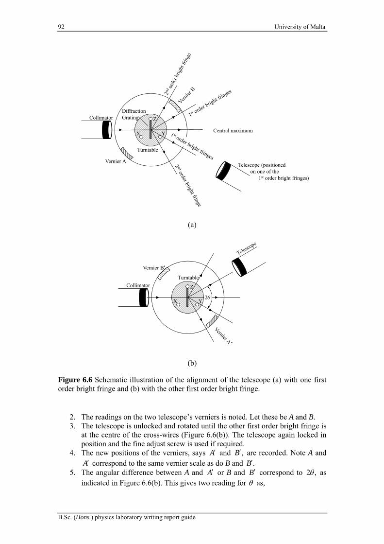
92 University of Malta
B.Sc. (Hons.) physics laboratory writing report guide
(a)
(b)
Figure 6.6 Schematic illustration of the alignment of the telescope (a) with one first order bright fringe and (b) with the other first order bright fringe.
2. The readings on the two telescope’s verniers is noted. Let these be A and B. 3. The telescope is unlocked and rotated until the other first order bright fringe is
at the centre of the cross-wires (Figure 6.6(b)). The telescope again locked in position and the fine adjust screw is used if required.
4. The new positions of the verniers, says A and ,B are recorded. Note A and A correspond to the same vernier scale as do B and .B
5. The angular difference between A and A or B and B correspond to 2 , as indicated in Figure 6.6(b). This gives two reading for as,
Turntable
Collimator
X Y
Z
Telescope (positioned on one of the
1st order bright fringes)
Central maximum
Vernier A
DiffractionGrating
Turntable
Collimator
X Y
Z
Vernier B′
2

Department of Physics 93
Chapter 6 Instrumentation
1 2
A A
and 2 .2
B B
Note that it may occur that on moving the telescope the reading exceeds 360 or goes below 0 . In such cases you should add or subtract 360 as necessary to determine a value for 1 or 2. You can easily determine if this is the case
if 1 and 2 are not approximately equal.
6. The average angle can now be found as, 1 2 .2
6.1.5 Using a prism
In the case of a prism, we need to ensure that the turntable is levelled before we make any measurement. However, before discuss the steps needed to make this setting you should make sure that you know how to take a reading from the vernier scales (see Section 6.1.3) and be familiar with the components of the spectrometer (see Figure 6.1). In particular you should note that the turntable has three adjustable levelling screws that can be accessed from below. These will be used to level the turntable.
The steps you need to follow in order to setup the spectrometer for use with a prism are as follows:
1. Make sure that the turntable is clear so that the path of the beam is unobstructed.
2. Align the telescope with the collimator (Figure 6.7(a)) and position the beam such that it is at the centre of the cross-wires (Figure 6.7(b)). You can lock the telescope in position using its lock screw and fine tune if necessary using the fine adjust screw. (See Figure 6.1 for the location of these components).
3. Keeping the telescope locked in position, note the position of the telescope from the telescope’s vernier.
4. Add or subtract 90 to the position of the telescope to determine the angle at which the telescope would be perpendicular to the collimator.
5. Unlock the telescope and, using the angle calculated in Step 4, position it at right angle to the collimator as shown in Figure 6.7(c). You can use the lock and fine adjusted screw to help you. Once finished leave the telescope locked.
6. Lock the turntable with its base using the lock screw (see Figure 6.1). 7. Place the prism such that its length is perpendicular to the line joining two
levelling screws. This is schematically illustrated in Figure 6.7(c) where the grating is at right angles to the line joining screws X and Y. Note that many spectrometers offer a support structure for prisms that can be attached to the turntable. This ensures that the prism will not move.
8. Rotate the turntable until the light reflected from side PQ of the prism is positioned in the centre of view of the telescope as shown in Figure 6.7(d).
9. Lock the turntable base in position using its lock screw and fine adjust using its fine adjust screw as necessary (see Figure 6.1) to place the beam at the centre of the cross-wires. Keep the turntable base locked.

94 University of Malta
B.Sc. (Hons.) physics laboratory writing report guide
(a) (b)
(c) (d)
(e)
Figure 6.7 (a) Top view of the aligned collimator and telescope. (b) Beam at the centre of the cross-wires. (c) Top view of the telescope at right angles to the collimator; the prism is placed with PQ perpendicular to the line joining levelling screws X and Y. (d) The light from the collimator is reflected from side PQ and enters the field of view of the telescope. (e) The light from the collimator is reflected from side QR and enters the field of view of the telescope.
10. At this point, if the grating is not perfectly vertical the beam will be displaced upward or downwards with respect to the cross-wires. In order to align the centre of the beam with that of the cross wires (Figure 6.7(b)) you can use screws X. Do not touch screws Y and Z.
11. Unlock the turntable base and rotate it until the light reflected from side QR is in the field of view of the telescope (Figure 6.7(e)). Lock the turntable base in position and fine adjust as required to get the image on the cross wires. Keep the turntable based locked in position once finished.
Turntable
Collimator
X Y
Z Telescope BeamCross-wires
Turntable
Collimator
X Y
Z
Telescope(at right angles to the collimator)
Prism (placed with face PQperpendicularly to screws X and Y)R
Q
P
Turntable
Collimator
XY
Z
Telescope
Prism
RQ
P
Turntable
Collimator
X
Y
Z
Telescope
Prism
R
Q
P

Department of Physics 95
Chapter 6 Instrumentation
12. Once again, if the table is not perfectly vertical the beam will be displaced upward or downwards with respect to the cross-wires. In order to align the centre of the beam with that of the cross wires (Figure 6.7(b)) you need to use screws Z. Do not touch screws X and Y. This adjustment will move side PQ in its plane so that it will not affect the previous adjustment.
13. The turntable is now levelled and the spectrometer ready for use.
The step up can now be used to measure for example the apex angle or the angle of minimum deviation. The relevant procedure will not be treated here but can be found in standard textbooks such as Muncaster (1993) or Nelkon and Parker (1970).


Department of Physics 97
References
References
Miller, I. and Miller M. (1999), John E. Freund’s Mathematical Statistics, sixth edition, Prentice Hall: New Jersey, USA.
Muncaster, R. (1993), A-Level Physics, fourth edition, Nelson Thornes Ltd.: Cheltenham, UK.
Nelkon, M. and Parker, P. (1970). Advanced Level Physics, third edition, Heinemann Educational Books Ltd: London, UK.
Squires G.L. (2001), Practical Physics, fourth edition, Cambridge University Press: Cambridge, UK.
Taylor J.R. (1997), An Introduction to Error Analysis the Study of Uncertainties in Physical Measurements, second edition, University Science Books: California, USA.