university of southampton research repository eprints soton › 30238 › 1 ›...
TRANSCRIPT

University of Southampton Research Repository
ePrints Soton
Copyright © and Moral Rights for this thesis are retained by the author and/or other copyright owners. A copy can be downloaded for personal non-commercial research or study, without prior permission or charge. This thesis cannot be reproduced or quoted extensively from without first obtaining permission in writing from the copyright holder/s. The content must not be changed in any way or sold commercially in any format or medium without the formal permission of the copyright holders.
When referring to this work, full bibliographic details including the author, title, awarding institution and date of the thesis must be given e.g.
AUTHOR (year of submission) "Full thesis title", University of Southampton, name of the University School or Department, PhD Thesis, pagination
http://eprints.soton.ac.uk
UNIVERSITY OF SOUTHAMPTON
Faculty of Engineering and Applied Science
Department of Electronics and Computer Science
All-Fibre Devices for WDM Optical Communications
by
Carlos Feio Gama Alegria
A thesis submitted for the degree of
Doctor of Philosophy
DECEMBER 2001
UNIVERSITYOFSOUTHAMPTONABSTRACT
FacultyofEngineeringandAppliedScienceDepartmentofElectronicsandComputerScience
DoctorofPhilosophy
ALL-FIBREDEVICESFORWDMOPTICALCOMMUNICATIONSbyCarlosFeioGamaAlegria
This thesis is concerned with the study of two key technologies for enablingwavelength division multiplexed optical communication systems. The first is gainequalisation of the erbium-doped fibre amplifier and the second is the routing ofoptical channels through the network by means of all-fibre add-drop multiplexerconfigurations. Firstly, in order to flatten dynamically the EDFA gain spectrum, an AO filterbased on a multi-tapered fibre structure was demonstrated. The controlled taperprofilewasusedasanotherdegreeoffreedomfortailoringthefilterlossspectrum.Thecouplingbetweenthefundamentalandseveralcladdingmodeswasinvestigatedbystudyingtheevolutionoftheresonanceconditionsasthefibresareprogressivelytapered both theoretically and experimentally. The filter was demonstrated byequalising the EDFA gain spectrum for different saturation levels. The mainadvantage of this novel design when compared to alternative AO filters is itssimplicityduetothereducednumberoftuningparameters.Furthermore,amethodof determining the ideal filter loss spectrum and correct placement within theamplifierwasanalysed.ThisisbasedoncalculatingtheEDFwavelengthdependentbackgroundlossnecessarytoequalisetheamplifiergainspectrum,andintegratingitintoadiscretenumberof filtersplacedwithin theEDFA.Configurationsbasedonone and two equalising filters were compared. Additionally, this method allowednovelcomplexfilterdesigns,whichcouldcompensatefortheirowninsertionlossesaswellastheinsertionlossesofotherdevicesdistributedalongtheamplifier,whileachievingaflatgainspectrum. Secondly, all-fibre OADMs based on the inscription of Bragg gratings in thewaist of fused fibre-couplers were investigated. Design considerations of devicesbased on half- and full-cycle couplers were presented and their performancescompared. Inboththeseconfigurationstheexactpositioningof thegratingswithinthe fused coupler waist is critical to achieve optimum performance. An all-fibrecompact add-drop multiplexer based on a novel non-uniform half-cycle fusedcoupler is presented, providing an alternative OADM design with optimisedsymmetricoperation,whichisinsensitivetothepositionofthegratinginthecouplerwaist.Thespectralperformanceofthis3cmlongdeviceissimilartothatofadevicebasedonameter-longuniformhalf-cyclecoupler.Finally,atechniqueforthenon-destructivecharacterisationofcouplers isproposed, inorder todetermine the3dBpoints within the couplers waist. A CO2 laser beam is scanned along the couplerlength inducing a local perturbation to the coupler eigenmodes. Asymmetric andsymmetricperturbationscangiveaccuratemappingofpower-evolutionandcoupler-waistshape.
Contents
Acknowledgments………………………………………………………..…..viii
I INTRODUCTIONCONTENTS............................................................................................................... III
1THESISOVERVIEW............................................................................................ 2
1.1 WAVELENGTHDIVISIONMULTIPLEXING ..................................................... 3
1.2 MOTIVATION ................................................................................................ 4
1.3 MAINACHIEVEMENTS.................................................................................. 5
1.4 SUMMARYOFTHETHESIS............................................................................. 6
2INTRODUCTIONTOTHEEDFA...................................................................... 8
2.1 EDFAOVERVIEW ........................................................................................ 9
2.2 THEORY ..................................................................................................... 10
2.2.1 Energy levels ..................................................................................... 10
2.2.2 Numerical modelling of spectral properties...................................... 13
2.3 NOISEFIGURE............................................................................................. 15
2.4 LARGERBANDWIDTH ................................................................................. 17
2.5 GAINEQUALISATION .................................................................................. 18
2.6 SUMMARY .................................................................................................. 20

iv
3INTRODUCTIONTOADD-DROPMULTIPLEXERS.................................. 21
3.1 OPTICALADD-DROPTECHNOLOGY ........................................................... 22
3.2 ADD-DROPCONFIGURATIONS .................................................................... 23
3.2.1 ReconfigurableAdd-Drops ............................................................... 27
3.3 ADD-DROPPERFORMANCE ........................................................................ 28
3.3.1 IsolationandCrosstalk ..................................................................... 28
3.3.2 Insertionlosses.................................................................................. 29
3.3.3 Back-reflections................................................................................. 30
3.4 SUMMARY .................................................................................................. 31
4INTRODUCTIONTOFIBRE-COUPLERS..................................................... 32
4.1 COUPLERTECHNOLOGY ............................................................................. 33
4.2 THEORETICALCOUPLERDESCRIPTION....................................................... 33
4.3 FABRICATIONOFFUSEDFIBRECOUPLERS ................................................. 37
4.3.1 Flame-BrushTechnique .................................................................... 37
4.3.2 CO2Laser.......................................................................................... 40
4.3.3 HeatingOven..................................................................................... 41
4.3.4 ShapeoftheTaperedRegion ............................................................ 41
4.3.5 Effectofthetaperedtransitiononthecouplerpowerevolution....... 44
4.3.6 Couplercrosssection ........................................................................ 48
4.4 SUMMARY .................................................................................................. 48
5INTRODUCTIONTOFIBREBRAGGGRATINGS...................................... 50
5.1 PHASEMATCHINGCONDITIONS ................................................................. 51
5.2 MATHEMATICALDESCRIPTIONOFBRAGGGRATINGS................................ 53
5.2.1 Coupledmodeequations ................................................................... 53
5.3 APODISATION ............................................................................................. 57
5.4 TRANSFERMATRIX .................................................................................... 60
5.5 PHOTOSENSITIVITY .................................................................................... 61
5.6 SUMMARY .................................................................................................. 62
v
II EDFAGAINEQUALISATION
6ACOUSTO-OPTICTUNABLEFILTERDESIGN ......................................... 63
6.1 ACOUSTO-OPTICTECHNOLOGY .................................................................. 64
6.2 THEORY ..................................................................................................... 66
6.2.1 Propagationoftheacousticwave ..................................................... 66
6.2.2 Opticalmodesintaperedfibres ........................................................ 68
6.2.3 Acousto-opticinteraction .................................................................. 71
6.3 EXPERIMENTS............................................................................................. 77
6.3.1 Characterisationofthedispersionrelations..................................... 78
6.3.2 FlatteningtheEDFAASEspectrum.................................................. 81
6.4 SUMMARY .................................................................................................. 86
7IDEALFILTERDESIGNFOREDFAGAINEQUALISATION.................. 88
7.1 INTRODUCTION........................................................................................... 89
7.1.1 TheoreticalModel ............................................................................. 90
7.2 THEORETICALFILTERDESIGN: ................................................................... 90
7.2.1 Effectofthefibrebackgroundloss.................................................... 92
7.3 DESIGNOFPRACTICALFILTERS .................................................................. 97
7.3.1 Idealfilter–Noinsertionloss........................................................... 97
7.3.2 Inclusionofthefilterinsertionloss................................................. 108
7.3.3 Filterdesignscompensatingthedeviceowninsertionloss ............ 113
7.3.4 EDFAEqualisationbyusingtheinverseofthegainspectrum....... 120
7.3.5 Conclusions ..................................................................................... 122
7.4 GAINFLATTENINGFILTERSCOMPENSATINGFORTHEINSERTIONLOSSESOF
OTHERDEVICES .................................................................................................... 124
7.4.1 EqualisationoftheEDFAwithalumplosspositionedatZ=2m ... 125
7.4.2 Equalisationofa(EDFA+isolator)structure: ............................. 132
7.4.3 Conclusions ..................................................................................... 137
7.5 SUMMARY ................................................................................................ 137
vi
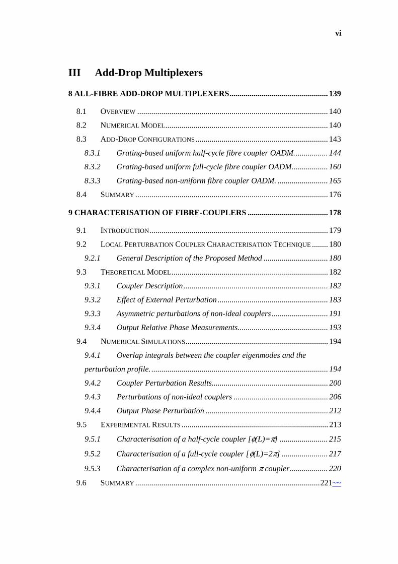
III Add-DropMultiplexers
8ALL-FIBREADD-DROPMULTIPLEXERS................................................. 139
8.1 OVERVIEW ............................................................................................... 140
8.2 NUMERICALMODEL................................................................................. 140
8.3 ADD-DROPCONFIGURATIONS .................................................................. 143
8.3.1 Grating-baseduniformhalf-cyclefibrecouplerOADM................. 144
8.3.2 Grating-baseduniformfull-cyclefibrecouplerOADM.................. 160
8.3.3 Grating-basednon-uniformfibrecouplerOADM. ......................... 165
8.4 SUMMARY ................................................................................................ 176
9CHARACTERISATIONOFFIBRE-COUPLERS ........................................ 178
9.1 INTRODUCTION......................................................................................... 179
9.2 LOCALPERTURBATIONCOUPLERCHARACTERISATIONTECHNIQUE ........ 180
9.2.1 GeneralDescriptionoftheProposedMethod ................................ 180
9.3 THEORETICALMODEL.............................................................................. 182
9.3.1 CouplerDescription........................................................................ 182
9.3.2 EffectofExternalPerturbation ....................................................... 183
9.3.3 Asymmetricperturbationsofnon-idealcouplers ............................ 191
9.3.4 OutputRelativePhaseMeasurements............................................. 193
9.4 NUMERICALSIMULATIONS....................................................................... 194
9.4.1 Overlapintegralsbetweenthecouplereigenmodesandthe
perturbationprofile. ........................................................................................ 194
9.4.2 CouplerPerturbationResults.......................................................... 200
9.4.3 Perturbationsofnon-idealcouplers ............................................... 206
9.4.4 OutputPhasePerturbation ............................................................. 212
9.5 EXPERIMENTALRESULTS ......................................................................... 213
9.5.1 Characterisationofahalf-cyclecoupler[φ(L)=π] ........................ 215
9.5.2 Characterisationofafull-cyclecoupler[φ(L)=2π] ....................... 217
9.5.3 Characterisationofacomplexnon-uniformπcoupler................... 220
9.6 SUMMARY ............................................................................................221~~
vii
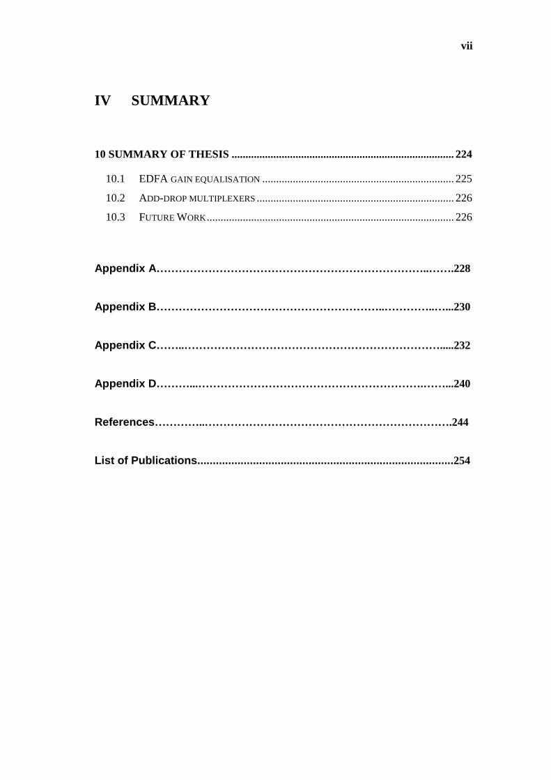
IV SUMMARY
10SUMMARYOFTHESIS ................................................................................ 224
10.1 EDFAGAINEQUALISATION ..................................................................... 225
10.2 ADD-DROPMULTIPLEXERS ....................................................................... 226
10.3 FUTUREWORK......................................................................................... 226
Appendix A… … … … … … … … … … … … … … … … … … … … … … … … ..… … .228
Appendix B… … … … … … … … … … … … … … … … … … … … ..… … … … ..… ...230
Appendix C… … ..… … … … … … … … … … … … … … … … … … … … … … … .....232
Appendix D… … … ...… … … … … … … … … … … … … … … … … … … … .… … ...240
References… … … … ..… … … … … … … … … … … … … … … … … … … … … … .244
List of Publications...................................................................................254
viii
Acknowledgements
During my studies at the ORC of the University of Southampton I have had the
pleasuretoworkanddiscussdifferentaspectsofoptoelectronicswithextraordinary
people.IamgratefultoProf.D.Payneforgivingmetheopportunityofstudyingat
theORCand to thePortugueseFundaçãoparaaCiênciaeTecnologia for funding
myPhD.
Among other people that have passed by, or are still at the ORC, I’d like to
thank Prof. D. Richardson, Prof R. Eason and Dr. E. Tarbox for giving me
confidence in my work, M. Ibsen, Dr. Y. S. Kim, Dr. C. Renaud for useful
discussions,R.Haaksmanforallhislogisticalhelp,theORCsecretariesEveSmith
andHeatherSpencer forhelpingme innumerous situations. I’dalso like to thank
everyonewhichwhomIhaveworkeddirectlyinthelaboratoriesfromwhomIhave
acquiredmanytechnicalskills,namely,F.Ghiringhelli,G.Brambilla,M.Ibsen,Dr.
R.Feced,Dr.M.Gunning,Dr.M.Durkin,NielP.FaganandSimonButler.
In particular I couldn’t thank enough Dr. R. Feced for all his help during the
initialstagesofmyPhDandJ.MackenzieandDr.E.Tarboxforgoingoutoftheir
way, taking the task of proofreading my thesis. I am also grateful to Prof. M. N.
Zervas, forhisexcellent supervisionof theworkandcommentson the thesis, and
RichardLamingfororiginallyacceptingmeashisPhDstudent.
I am also very grateful to all my friends that in one way or another gave me
supportthroughoutmystayinSouthamptonandinparticular;Isabel,Ricardo,Jacob
and the Sparrows. Finally, I would like to thank my family for all their support
duringmyPhD,withoutwhomIwouldn’tbewritingtheselines.

1
ThesisOverview
1–ThesisOverview 3
1.1 WavelengthDivisionMultiplexing
The advent of the Internet and global spread of personal computers has
revolutionisedourwayoflifeinthelast10years.Theabilitytocommunicate,shop,
travel, find information, listen to radio, get medical support, and so many other
aspectsofthedaybydaylife,areaccessiblewithasimplemouse-click.Thedemand
forbettermultimediaservicesandtheincreasingnumberofInternetusershasgiven
rise to an increased demand on the optical network capacity and efficiency, in all
sectors - local area networks (LAN), metropolitan networks (METRO), and long-
haulsystems.Consequently,theneedtotransmitgreateramountsofinformationvia
a single optical fibre, coupled with the need for low cost and more efficient
distributionnodes inLAN[1],has led to the increasing importanceofwavelength
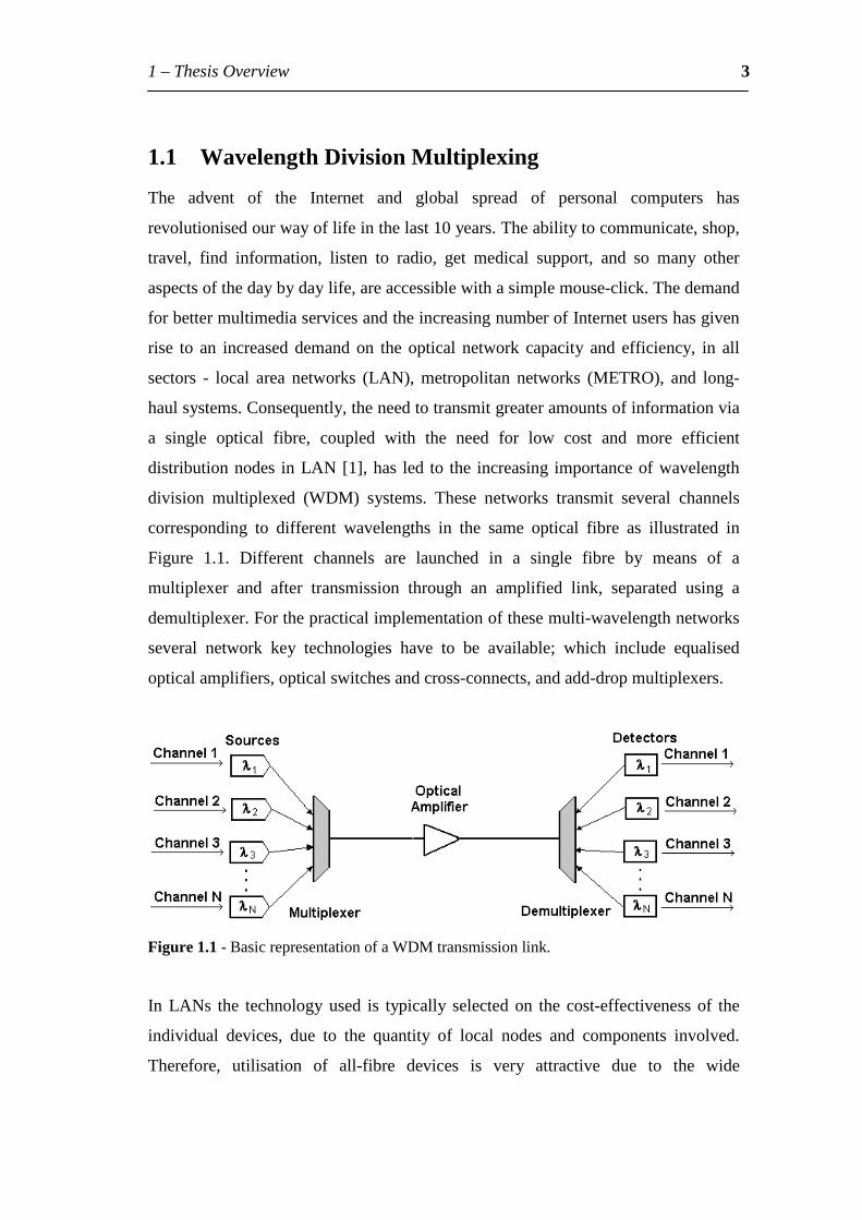
division multiplexed (WDM) systems. These networks transmit several channels
corresponding to different wavelengths in the same optical fibre as illustrated in
Figure 1.1. Different channels are launched in a single fibre by means of a
multiplexer and after transmission through an amplified link, separated using a
demultiplexer.Forthepracticalimplementationofthesemulti-wavelengthnetworks
several network key technologies have to be available; which include equalised
opticalamplifiers,opticalswitchesandcross-connects,andadd-dropmultiplexers.
Figure1.1-BasicrepresentationofaWDMtransmissionlink.
In LANs the technologyused is typically selectedon the cost-effectivenessof the
individual devices, due to the quantity of local nodes and components involved.
Therefore, utilisation of all-fibre devices is very attractive due to the wide
1–ThesisOverview 4
availability and relatively low cost of optical fibres; consequently significant
researchhasbeenaimedat thisarea.However, in long-haul transmissionsystems,
emphasis is given to long-term stability and performance of the technologies
employed. Recently the utilisation of fibre amplifiers operating at different
wavelength bands (S, L and C) led to a system trial that demonstrated a record
transmission capacity of 6.4Tbits/s using WDM technology [2]. In contrast, for
opticaltimedomainmultiplexing(OTDM)systemsthemaximumbitrateachieved
was1.28Tbit/s[3].
This thesis is aimed mainly at investigating two components used in WDM
systems namely; gain equalised erbium-doped fibre amplifiers (EDFAs) and all-
fibre add-drop multiplexer configurations. An acousto-optic tunable filter for the
dynamicequalisationoftheEDFAgainspectrumisdemonstratedandatheoretical
studyoftheidealfiltershapeandplacementintheamplifierisperformed.Different
add-drop configurations based on the inscription of gratings in the waist of fused
fibre-couplers are investigated and a novel device based on a non-uniform fibre
couplerisdemonstrated.Thesensitivityoftheperformanceofthesedevicesonthe
positioninthecouplerwaistwherethegratingiswritten,hasledtothedevelopment
ofanoveltechniqueforthecharacterisationoffibrecouplers.
1.2 Motivation
The main motivation for this research was to develop an understanding of the
aspects related to EDFA gain flattening and routing of signals in WDM optical
communicationsandtodemonstratenoveldevicesormethodsthatmaybeusedin
suchnetworks.Thekeytopicsunderlyingthisworkcanbesummarisedasfollows:
• Todevelopanunderstandingofthedesignandfabricationaspectsrelatedtoadd-
drop multiplexers based on a Bragg grating inscribed in the waist of a fibre-
coupler.
1–ThesisOverview 5
• TodevelopanunderstandingofEDFAgainequalisingfiltersandconfigurations
andtodemonstrateanacousto-optictunablefilterforequalisingtheEDFAgain
spectrumfordifferentamplifiersaturations.
• To demonstrate a compact all fibre add-drop multiplexer with symmetric
operation.
• Todeveloppersonalexperimental,research,engineeringandsoftwareskills.
1.3 MainAchievements
ThisthesisisfocusedmainlyontwoaspectsofWDMopticalcommunications:First
theneedfortheequalisationoftheEDFAgainspectrumandsecondlytheselective
routingofdifferentopticalchannelsbymeansofadd-dropmultiplexers.
Chronologicallytheworkwasinitiatedbydevelopinganacousto-optictunable
filter forequalising theEDFAgainspectrumunderdifferentsaturationconditions.
This device was demonstrated as a simple (easier to reconfigure) although less
flexible alternative to solving the problem. Secondly, a theoretical study of ideal
filters for the EDFA gain equalisation was performed giving an insight into the
possibilities and limitations for extrinsic filters placed either outside or within the
EDFA.
Thesecondaspectoftheworkwasdirectedtowardsthedemonstrationofnovel
add-dropmultiplexerdesignsbasedon inscriptionofgratings in thewaistof fibre
couplers. This project has led to an understanding of aspects related to the
performanceof thesedevicesandhowtheycanbeaddressedpractically.Firstly,a
novelmethodforcharacterisingfibre-couplersbasedonalocalperturbationinduced
by a CO2 laser beam was developed and secondly, a novel add-drop multiplexer
designwasdemonstrated.
DuringmyPhDstudiesnumerousfibre-couplershavebeenfabricatedandthen
inscribed UV induced Bragg-gratings in their waist. The procedure undertaken on
1–ThesisOverview 6
the fibre couplers from the time of fabrication was optimised during the work
according to the facilities available. A considerable amount of time has also been
spent modelling fibre propagation characteristics, add-drop multiplexers based on
fibre couplers with a grating inscribed in the waist, and the local perturbation of
fibrecouplers.
1.4 Summaryofthethesis
This thesis investigates two technologies essential for the deployment of WDM
networks.ThefirstisequalisationoftheEDFAgainspectrum,andthesecondisthe
routingofchannelsthroughall-fibreadd-dropmultiplexerconfigurations.Thethesis
isdividedinfoursections:
-SectionIisanintroductiontothedevicesandtechnologiesinvolvedinthisstudy.
Following this chapter, which puts this thesis into context and outlines the
motivation for the work, chapter 2 introduces the EDFA, and the different issues
relevant to its performance in optical networks. Chapter 3 discusses the add-drop
multiplexer,thedefiningparametersthatareusedtocharacterisetheirperformance
and addresses different configurations used for routing WDM channels. It also
reviews the technologies investigated to date and the advantages or drawbacks or
otherwise of each. Next, in chapter 4, fibre couplers are introduced, where the
understandingandoptimisationofthesedevicesisessentialforoptimisationofadd-
dropmultiplexerconfigurations investigated in this thesis.Couplersaloneare also
important components in WDM networks used to route, split, or combine optical
signalsandthereforeasignificantpartofthisthesisisdedicatedtothem.Theadd-
drop configurations investigated in this work rely on Bragg gratings for filtering
selected wavelengths; chapter 5 provides a brief introduction to these devices and
the subsequent issues related to this thesis. The second and third sections of this
thesisaretheauthor’ scontributiontotheareaofopticalcommunications.
1–ThesisOverview 7
-Section II addresses the equalisationof theEDFAgain spectrum. In chapter6 a
novel technique for tailoring the loss spectrum of an acoustooptic (AO) filter is
proposed. The application of the technique is demonstrated by dynamically
equalising the amplified spontaneous emission (ASE) spectrum of an EDFA for
different saturating input signals. The operation of the device relies on simpler
tuningconditionscomparedtosimilaralternativetechnologies.Chapter7presentsa
theoreticalandnumericalstudyofidealfiltersfortheequalisationoftheEDFAgain
spectrum.Itdiscussesamethodfordeterminingtherequiredidealfiltershapesand
placement position in the amplifier in order to obtain the best performance whilst
equalising the EDFA gain spectrum. It is shown that the optical filter can be
properly designed in order to compensate for its own insertion loss as well as of
otherdevicesincorporatedintheEDFA.
- Section III is dedicated to all-fibre add-drop multiplexer configurations. It
addresses three compact all-fibre configurations basedon the inscriptionof Bragg
gratings in the waist of fibre-couplers. Design and fabrication issues for each of
these configurations are addressed in chapter 8. The need for an experimental
methodforcharacterisingthefibre-couplers,inordertocorrectlypositiontheBragg
gratingswithin thecouplerwaist, led to thedevelopmentofanovel technique for
the non-destructive characterisation of fibre-couplers. This technique is based on
scanninga locally inducedperturbationalong thecouplerwaist toobtain the taper
andwaistprofileanddeterminetheevolutionofpoweralongthecoupler,aswellas,
theshapeofthecouplerwaistandcouplingconstantdistribution.Thisisaddressed
theoreticallyandexperimentallyinchapter9.
- SectionIVdrawsconclusionsregardingtheabove-mentionedtopics,concluding
withpossibledirectionsforthisresearchtocontinue.
2
IntroductiontotheEDFA
A general introduction to the EDFA is presented in this chapter. It starts with an
overview of the implementation of this component in optical communications
networks, thenabriefdescriptionof theamplifieroperationandhowtomodel the
spectral characteristics. Important amplifier parameters such as the optical noise
figure,amplifierbandwidth,andmethodstoachieveequalisationoftheEDFAgain
spectrumareintroduced.
2–IntroductiontotheEDFA 9
2.1 EDFAOverview
TheinventionoftheEDFAinthelateeighties[4,5]wasoneofthemajoreventsin
the history of optical communications. It provided new life to the optical fibre
transmission window centred at 1.55µm and the consequent research into
technologiesthatallowhighbit-ratetransmissionoverlongdistances.Highbit-rates
werealsopossiblewiththeaidofdifferentdispersioncompensationschemes.The
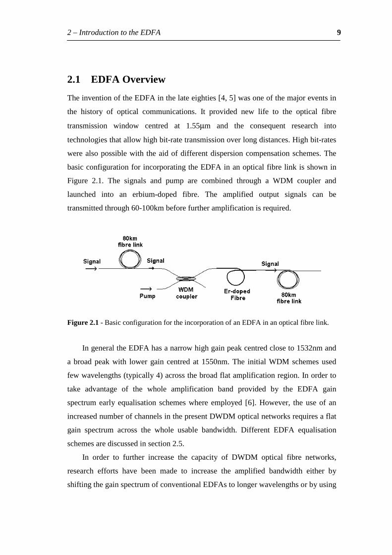
basicconfigurationforincorporatingtheEDFAinanopticalfibrelinkisshownin
Figure 2.1. The signals and pump are combined through a WDM coupler and
launched into an erbium-doped fibre. The amplified output signals can be
transmittedthrough60-100kmbeforefurtheramplificationisrequired.
Figure2.1-BasicconfigurationfortheincorporationofanEDFAinanopticalfibrelink.
IngeneraltheEDFAhasanarrowhighgainpeakcentredcloseto1532nmand
abroadpeakwith lowergain centred at 1550nm.The initialWDMschemesused
fewwavelengths(typically4)acrossthebroadflatamplificationregion.Inorderto
take advantage of the whole amplification band provided by the EDFA gain
spectrumearly equalisation schemeswhere employed [6].However, the useof an
increasednumberofchannelsinthepresentDWDMopticalnetworksrequiresaflat
gain spectrum across the whole usable bandwidth. Different EDFA equalisation
schemesarediscussedinsection2.5.
In order to further increase the capacity of DWDM optical fibre networks,
research efforts have been made to increase the amplified bandwidth either by
shiftingthegainspectrumofconventionalEDFAstolongerwavelengthsorbyusing
2–IntroductiontotheEDFA 10
newdopantsandglassestoprovideamplificationatdifferentwavelengthbands(see
section2.4)orbyusingRamanamplifiers.
EDFAs have been used successfully in WDM transmission systems as all-
opticallumpedamplifiersatwhichthegainisboostedatapointofthetransmission
line. On the other hand, the fibre amplifiers based on Raman effect also have
attracted huge research attention nowadays due to its tunability of amplification
bandbysimplychangingpumpwavelength,sinceever-increasingdemandofoptical
data transmission capacity expansion in telecommunications has generated
enormous interest inopticalcommunicationbands (S-,L-band) [7,8]outsideofa
conventionalEDFAgainbandwidth(C-band).TheprincipleoftheRamanamplifier
is based on the stimulated emission process associated with Raman scattering in
fibrefortheamplificationofsignals.Theinelasticnon-lineareffectscanberegarded
as scattering of a pump beam off phonon (molecular vibrational state) and the
transfer of energy into a lower energy beam. The Stokes shift corresponds to the
Eigen-energy of an optical phonon, which is approximately 13.2 THz for optical
fibres. InRamanamplifiers,signalwavelengthis longerthanpumpwavelengthby
the equivalent amountof the frequency shift. By usingmultiplepumps across the
targetgainwindow,over100nmbandRamanamplifierscanbeachieved [9].The
majordrawbacksofthistechnologyaretherequirementofhighpumppowerorlong
length of fibre and the related Rayleigh scattering issue. However, availability of
cheapandhighpowerpumplasers,andhighlynon-linearfibresenablesfibreRaman
amplifierstobeapromisingtechnologyfortheincreaseoftransmissioncapacityof
currentandfutureWDMnetworks.
2.2 Theory
2.2.1 Energylevels
TheEDFA absorption andemission cross sections are the signatureof the energy
levelsoftheEr3+ionintheglasshost.Whentheerbiumionisintroducedintoahost
2–IntroductiontotheEDFA 11
medium the energy levels are modified by local electric fields through Stark-
splitting. These levels are in thermal equilibrium due to rapid nonradiative
transitions between these levels. The amplifier is assumed to have homogeneous
broadeningbutifthelocalelectricfieldisdifferentatvarioussitesalongoracross
thefibreduetoimpurities,clusteringeffects,orotherglassstructuraldisorders,then
inhomogeneous broadening occurs resulting in different electronic transitions at
respectivesites.TheincorporationofanetworkmodifiersuchasAluminium(Al)to
enhance the solubility of the Er3+ ions in the glass structure changes each energy
level’ sStark-splittingandincreasestheinhomogeneityof themedium.Theenergy
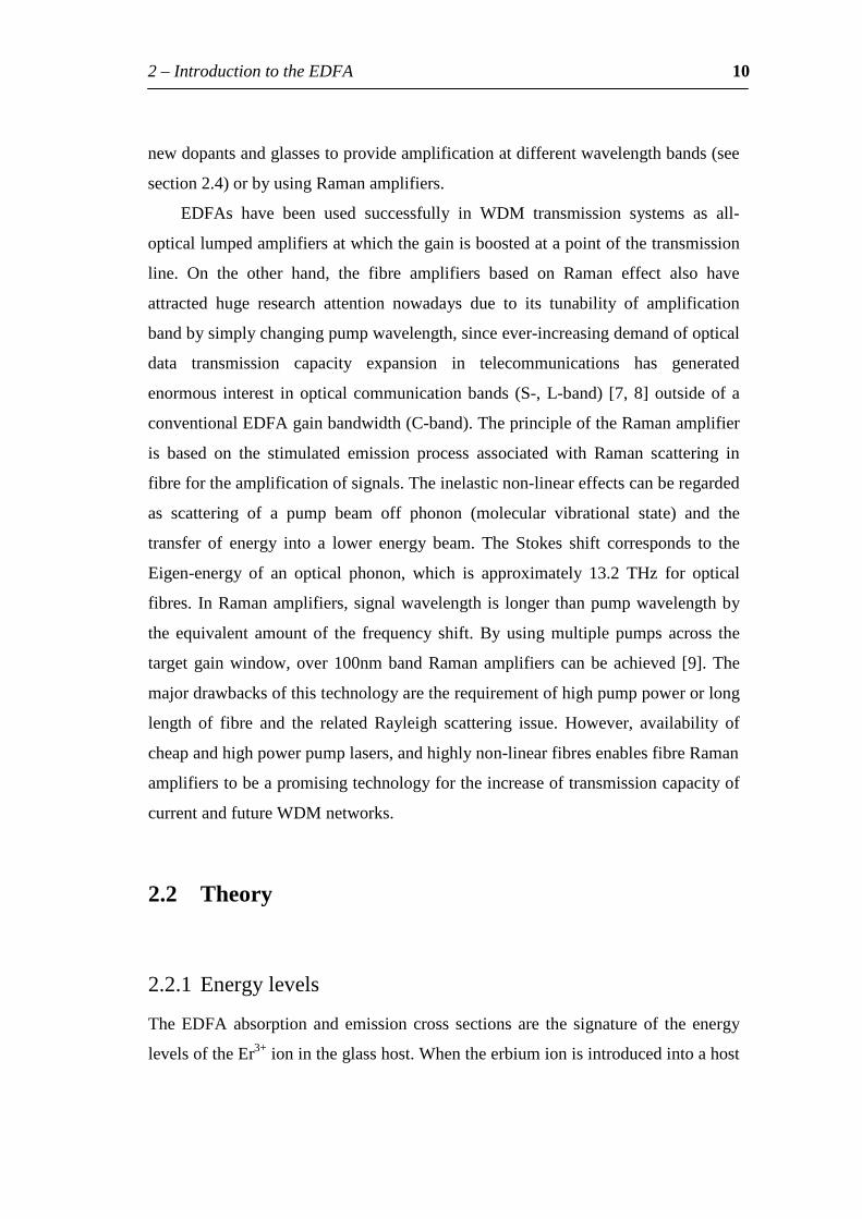
transitions typically associatedwithEr3+ ina silicateglassare the 4I11/2,4I13/2, and4I15/2states,andareillustratedinFigure2.2.
Figure2.2–a)Energy leveldiagram forEr3+ ions showing thedominant transitions. b)
Stark-splittingoftheenergylevelsduetothecrystalorglasselectricfield.
W12,W21aretheratesforthestimulatedtransitionswhileA32andA21aretherates
forthespontaneousemission.A32isassumedtobeessentiallynonradiativeandA21
essentially radiative [10].Thesubscripts1,2 and3correspond respectively to the
energylevels4I15/2,4I13/2,and4I11/2.
2–IntroductiontotheEDFA 12
GenerallytheEDFAispumpedwith980nmradiation,excitingelectronsfrom
the ground state 4I15/2 to level 4I11/2 or at 1480nm by exciting electrons from the
groundstatetoahigh-energyStark-splitsublevelofthe4I13/2manifold.Rigorously
this implies, when pumping the EDFA using a wavelength of 980nm, that the
amplifiercorrespondstoathree-levelsystemwhilewhenusinga1480nmpumpthe
amplifierisaquasithree-levelsystem(aspumpingistoahigher-energyStark-split
statewithin the I13/2manifold).However,bothpumpingschemescanbedescribed
effectivelyintermsofthepopulationsoftwolevels.Thisapproximationisjustified
inthe980nmpumpingcaseduetothenonradiativedecayrateA32beingmuchlarger
thanthestimulatedemissionratefrom3to1,andthereforethepopulationoflevel3
(4I11/2) can be neglected. In the case of 1480nm pumping the two-level system is
justified due to the rapid thermalisation decay that transfers the higher-energy
electronsof the4I13/2manifold to lower-energyStarksublevels.Therateequations
forthepopulationsofatwo-levelsystemarewrittenas:
2212211122 nAnWnW
dtdN −−= (2.1a)
21 nnnt += (2.1b)
wherentistheEr3+iondensityandn1andn2thefractionaldensityofthelowerand
upperexcitedlevelsrespectively.Theseequationsholdevenforthemorecomplex
system where the manifolds are split into Stark sublevels. In this situation the
transitionratescorrespond to thesumoverall thepossible j-k (j,k=1,2) transitions
multiplied by the population weight of the transition, given by the Boltzman
distribution[10]. Inpracticehowever theexactenergy levelscorresponding to the
individual Stark levels are dependent upon the ion distribution and host material.
Thusthepopulationanddecayratesfortheenergylevelsofinterest,typicallyhave
to be determined experimentally through absorption and emission cross section
measurements.
2–IntroductiontotheEDFA 13
2.2.2 Numericalmodellingofspectralproperties
The wavelength dependent properties of EDFAs can be modelled following the
method proposed by [11] in which the spatial characteristics of the amplifier are
integrated. This model involved dividing the EDFA spectrum into discrete optical
channels of frequency bandwidth, ∆νk, centred at the optical wavelength λk.
Assuming homogeneous broadening and a uniform distribution of the Er3+ ions
across the fibre core, the amplifier can be characterised by introducing four
measurablefibreparameters:Theabsorptionspectrum,αk,thegainspectrumg*k,the
fibresaturationpower,PkSat,andthefibrebackgroundloss,lk,thataregivenby:
tkekk ng Γ= σ* (2.2a)
tkakk nΓ= σα (2.2b)
** )( kk
k
kk
teffkSatk g
hg
nAhP
+=
+=
αξν
ταν
(2.2c)
Where; σak and σek are respectively the wavelength dependent absorption and
emissioncrosssections,ntisthetotalconcentrationoftheerbiumions,ξ=Aeffnt/τis
theratioofthelineardensityoferbiumionstothefluorescencelifetime,Aeff=πb2eff
istheeffectiveareaofthedopedregion,τisthemetastablelevel2lifetime,andΓk
istheoverlapintegralbetweenthedopantandopticalmodedistributionsthatinthe
caseofuniformdopingoftheerbiumions(beff=b)isgivenby:
=Γπ
φφ2
0 0
),(b
kk rdrdrI (2.3)
WherebistheradiusoftheEr3+-dopedregion.Ifthisassumptionisunrealisticthen
modification of the integral is required to include the Er3+ ion distribution. The
2–IntroductiontotheEDFA 14
aboveoverlapintegraldependsingeneralonthewavelengthchannel,k,forwhichit
iscalculated.Understeady-stateoperation,assumingauniformdistributionfor the
excitedlowerstateandupperstatepopulations(n1andn2respectively),theexcited
upperstatepopulationdensityfortheEDFAisgivenby[11]:
+
+=
kSat
k
k
kSat
k
k
kk
k
t
PzPP
zPg
nn
)(1
)(*
2 αα
(2.4a)
21 nnnt += (2.4b)
Theequationsthatdescribethepropagationofthebeamsofwavelengthλkandthe
pumpthroughthefibreare[10]:
( ) ( )
+−∆++= )()( 2*2* zPlmh
nn
gzPnn
gudzdP
kkkkkt
kkt
kkkk αννα (2.5a)
( ) ( )
+−+= )()(2* zPlzP
nn
gudz
dPpumppumppumppump
tpumppumpk
pump αα (2.5b)
Pk(z) is the signal power at frequency λk at a certain position along the amplifier
length; uk represents the direction of the travelling beam uk=1 for a forward
propagating beam and uk=-1 for backward propagation; the term mhνk∆νk is the
contributionofthespontaneousemissionfromthelocalexcitedstatepopulationn2,
withm=2correspondingtothenumberofpolarisationmodessupportedbythefibre,
andh thePlankconstant; lk is awavelengthdependentbackground loss.Thus the
two-level amplifier system can be fully characterised using equations (2.5a) and
(2.5b)thatdescribethepropagationofthesignal,ASEandpumpalongtheerbium-
dopedfibreandequation(2.4.a)describingthepopulationinversionandsaturation
characteristicsalong theamplifier.Whenusing apumpwavelengthof980nm, the
2–IntroductiontotheEDFA 15
gaincoefficient isnull 0g*980 = andequation(2.5b)describingthepumpevolution
alongtheEDFcanbesimplified.
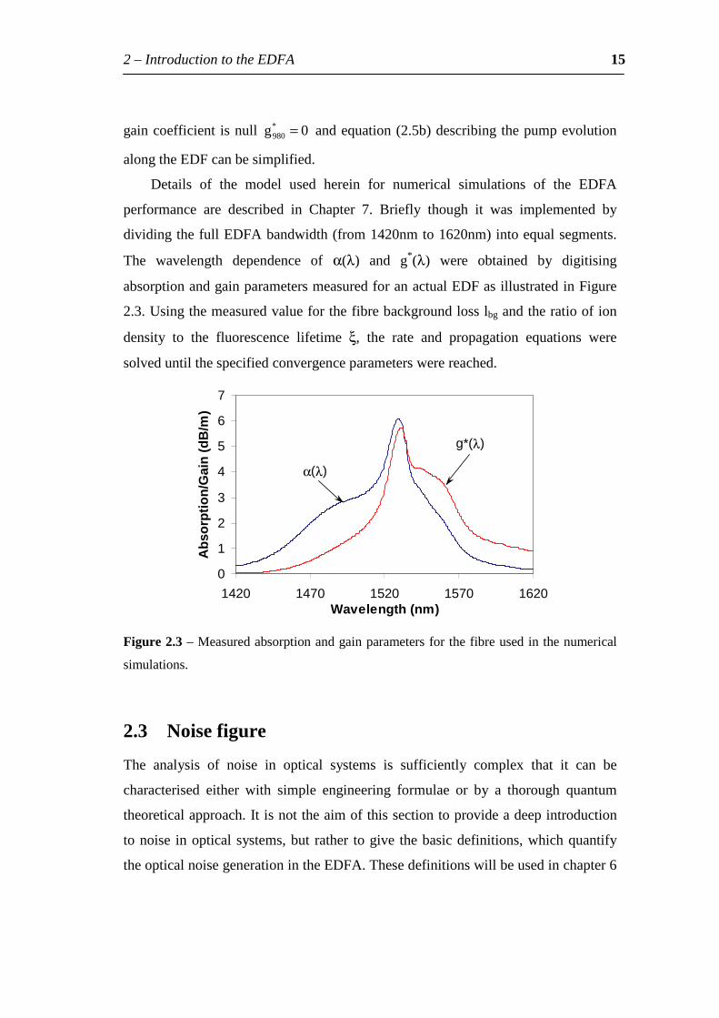
Details of the model used herein for numerical simulations of the EDFA
performance are described in Chapter 7. Briefly though it was implemented by
dividingthefullEDFAbandwidth(from1420nmto1620nm)intoequalsegments.
The wavelength dependence of α(λ) and g*(λ) were obtained by digitising
absorptionandgainparametersmeasuredforanactualEDFasillustratedinFigure
2.3.Usingthemeasuredvalueforthefibrebackgroundlosslbgandtheratioofion
density to the fluorescence lifetime ξ, the rate and propagation equations were
solveduntilthespecifiedconvergenceparameterswerereached.
0
1
2
3
4
5
6
7
1420 1470 1520 1570 1620Wavelength(nm)
Abs
orpt
ion/
Gai
n(d
B/m
)
g*(λ)
α(λ)
Figure2.3–Measuredabsorptionandgainparametersforthefibreusedinthenumerical
simulations.
2.3 Noisefigure
The analysis of noise in optical systems is sufficiently complex that it can be
characterised either with simple engineering formulae or by a thorough quantum
theoreticalapproach.Itisnottheaimofthissectiontoprovideadeepintroduction
tonoise inopticalsystems,but rather togive thebasicdefinitions,whichquantify
theopticalnoisegenerationintheEDFA.Thesedefinitionswillbeusedinchapter6
2–IntroductiontotheEDFA 16
todiscusstheeffectontheEDFAperformance,intermsofanoisefigure,whenthe
concept of gain equalising filters is introduced. The optical noise figure is a
parameter used for quantifying the noise penalty added to a signal due to the
insertionofanopticalamplifier.Thatis,beforelightentersanamplifierthesignalto
noiseratioisSNR(0),afteramplificationitisSNR(z).Thus,opticalnoisefigurecan
bedefinedas:
)()0(
zSNRSNR
NFOpt = (2.6)
Ifthenoisefigureoftheamplifierwere1,thentheinitialsignaltonoiseratiowould
be maintained throughout amplification. However it has been shown that the
quantumlimitforanopticalamplifier[10]is3dB,thereforethesignaltonoiseratio
afteramplificationishalf(50%)oftheoriginalvalue.Forrealopticalamplifiersthe
noise figure can be as high as 6dB whereby the signal quality is sufficiently
deteriorated that the detector’ s ability to discriminate signal from noise is
compromised.
The signal to noise ratio can be described as the ratio between the average
signal intensity and the standard deviation of intensity fluctuations from that
average.Thedefinition follows in termsof theaveragenumberofphotons<n(z)>
andthevarianceσ2=<n(z)2>-<n(z)>2:
)(
)(2
2
z
znSNR
σ= (2.7)
wherezisthepositionalongtheamplifierorfibrelink.Ithasalsobeenshown,[10]
thatthenoisefigureofanopticalamplifiercanbedescribedas:
)(1
)(1)(
2zGzG
zGnNF
kk
kspOpt +−= (2.8)
2–IntroductiontotheEDFA 17
whereGk(z)istheamplifiergainatagivenposition,z,atawavelengthλkandwhere
nspisthespontaneousemissionfactorthattakestheform:
12
2
NN
Nn
ek
aksp
σσ−
= (2.9)
Here, N1 and N2 are the populations of the ground and excited energy levels
respectively. For a total population inversion N1=0, nsp=1 and therefore the noise
figure is close to 2, which is the quantum limit for the amplifier noise. The
spontaneous emission factor is related to the total power of the amplified
spontaneousemissionPASEwithinthebandwidth,∆νk,bythefollowingexpression
[10]:
( ) kk
ASEsp hG
Pn
νν∆−=
12 (2.10)
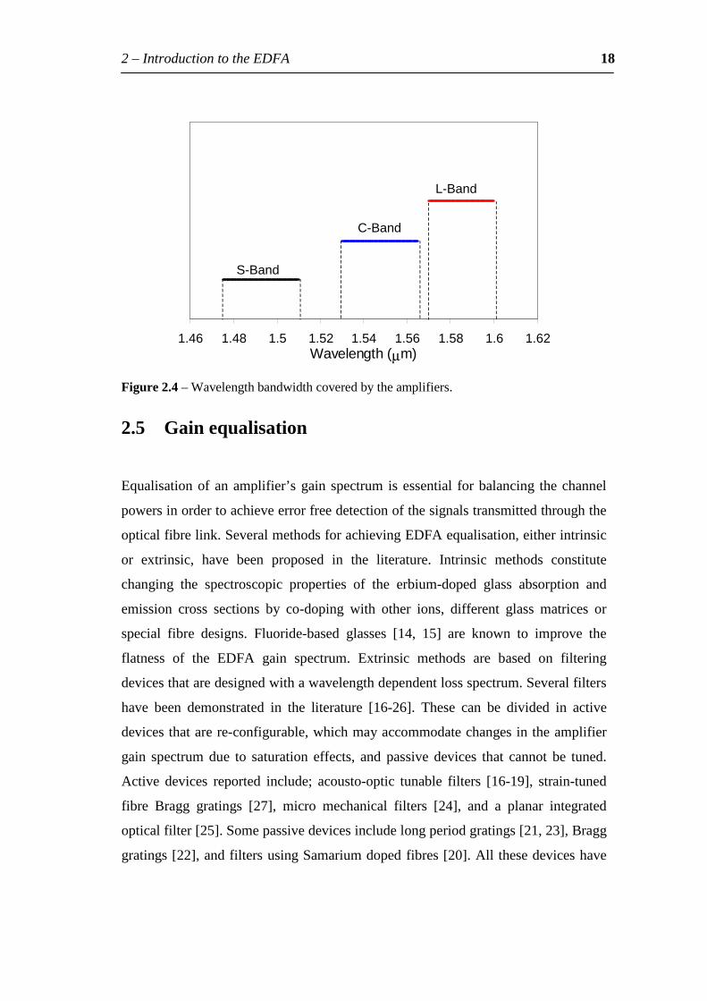
2.4 Largerbandwidth
Theusable35nmbandwidthof theEDFAoperating in theConventionalband (C-
Band)enabled fibre communicationsusingWDMandDWDM.Howevergrowing
demand for increased bandwidth and subsequent research have given rise to fibre
amplificationatshorterandlongerwavelengthbands.TheL-bandEDFA,wherethe
EDFA gain is shifted to the longer wavelengths (1560nm-1580nm) [12], in
conjunctionwiththerecentlydemonstratedThulium-dopedfibreamplifieroperating
attheS-band(shortwavelengths)around1490nm[13],providethebasisforfuture
transmission capacity of 10Tbits/s channels multiplexed across the three amplifier
bands [2].Figure2.4 illustrates the threeamplificationbandwidthscoveredby the
threetypesofamplifiers.
2–IntroductiontotheEDFA 18
1.46 1.48 1.5 1.52 1.54 1.56 1.58 1.6 1.62Wavelength (µm)
L-Band
S-Band
C-Band
Figure2.4–Wavelengthbandwidthcoveredbytheamplifiers.
2.5 Gainequalisation
Equalisationofanamplifier’ s gain spectrum isessential forbalancing thechannel
powersinordertoachieveerrorfreedetectionofthesignalstransmittedthroughthe
opticalfibrelink.SeveralmethodsforachievingEDFAequalisation,eitherintrinsic
or extrinsic, have been proposed in the literature. Intrinsic methods constitute
changing the spectroscopic properties of the erbium-doped glass absorption and
emission cross sections by co-doping with other ions, different glass matrices or
special fibre designs. Fluoride-based glasses [14, 15] are known to improve the
flatness of the EDFA gain spectrum. Extrinsic methods are based on filtering
devicesthataredesignedwithawavelengthdependentlossspectrum.Severalfilters
have been demonstrated in the literature [16-26]. These can be divided in active
devicesthatarere-configurable,whichmayaccommodatechangesintheamplifier
gain spectrum due to saturation effects, and passive devices that cannot be tuned.
Active devices reported include; acousto-optic tunable filters [16-19], strain-tuned
fibre Bragg gratings [27], micro mechanical filters [24], and a planar integrated
opticalfilter[25].Somepassivedevicesincludelongperiodgratings[21,23],Bragg
gratings[22],andfiltersusingSamariumdopedfibres[20].Allthesedeviceshave
2–IntroductiontotheEDFA 19
characteristicequalisationpropertiesand insertion losses thatcanbeas lowas the
splicinglossbetweentheEDFfibreandthefilterfibreorashigh8-9dBasreported
in[24,25].
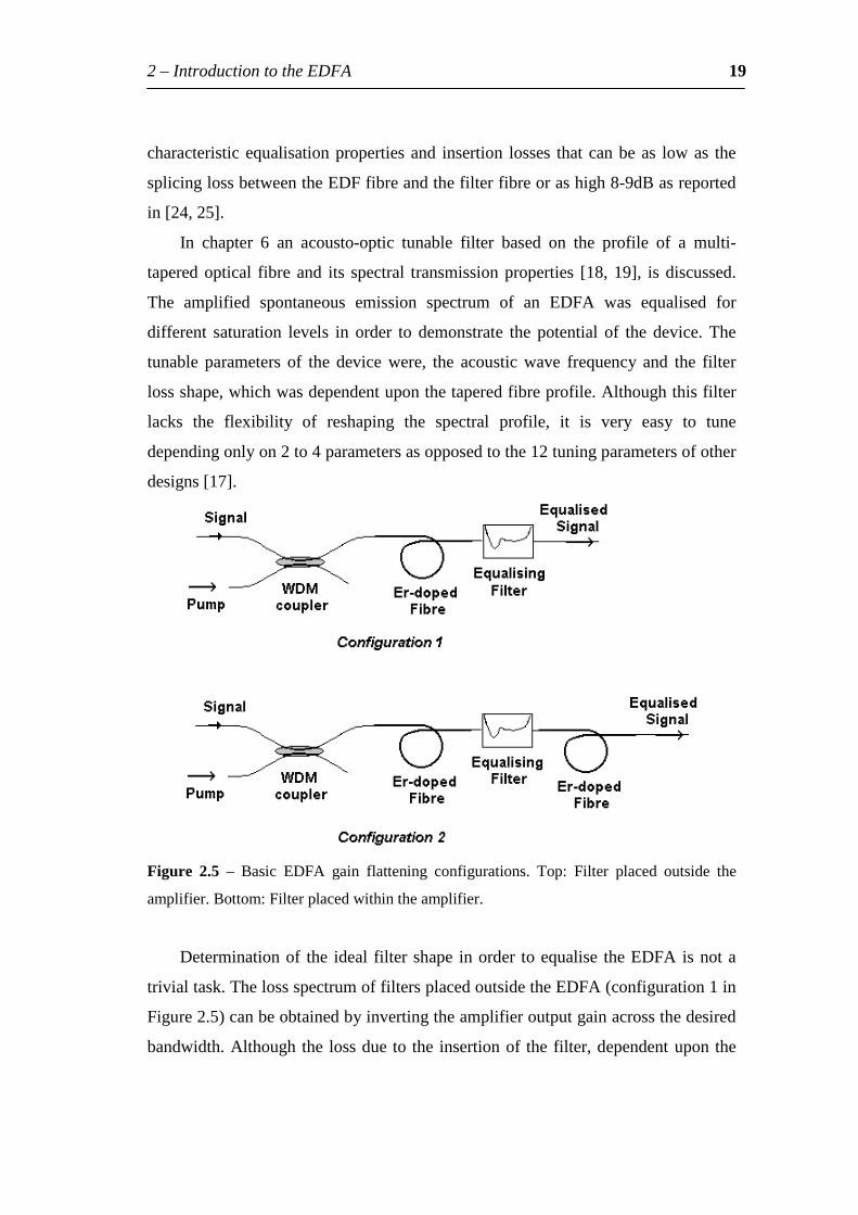
In chapter 6 an acousto-optic tunable filter based on the profile of a multi-
taperedoptical fibre and its spectral transmissionproperties [18,19], isdiscussed.
The amplified spontaneous emission spectrum of an EDFA was equalised for
different saturation levels in order to demonstrate the potential of the device. The
tunable parameters of the device were, the acoustic wave frequency and the filter
lossshape,whichwasdependentuponthetaperedfibreprofile.Althoughthisfilter
lacks the flexibility of reshaping the spectral profile, it is very easy to tune
dependingonlyon2to4parametersasopposedtothe12tuningparametersofother
designs[17].
Figure 2.5 – Basic EDFA gain flattening configurations. Top: Filter placed outside the
amplifier.Bottom:Filterplacedwithintheamplifier.
Determinationof the ideal filtershape inorder toequalise theEDFAisnota
trivialtask.ThelossspectrumoffiltersplacedoutsidetheEDFA(configuration1in
Figure2.5)canbeobtainedbyinvertingtheamplifieroutputgainacrossthedesired
bandwidth.Althoughthelossduetotheinsertionof thefilter,dependentuponthe
2–IntroductiontotheEDFA 20
type of filter and the fabrication procedure, can be up to 8-9dB [24, 25], and
thereforeanotheramplificationstageisusuallyrequiredafterthefilter.Ifhowever,
thefilterisplacedatacertainpositioninsidetheEDFA(configuration2inFigure
2.5), the penalty in amplifier loss can be reduced but the exact filter shape and
placement is not known. Liaw [20] used the loss spectrum of a samarium-doped
fibreandfoundthebestpositionatwhichitshouldbeplacedinagivenamplifierby
splicingitatdifferentpositionsalongtheamplifier.Acoustooptictunablefilters[26]
have alsobeenused in this configuration andoptimisedby tuning the filter shape
untilthedesiredperformanceisreached.Thisisaniterativeprocessandquitetime
consuming, as the filters may not be placed in the optimum position along the
amplifier. A solution to these problems is proposed in chapter 7, where the
theoreticaldesignofidealfiltersthatinadditiontogainflatteningalsocompensate
forinsertionlosses,andtheirpositionwithinanamplifierforequalisingtheEDFA
gain spectrum is discussed. Performance of the above filter configurations is
compared.
2.6 Summary
AbriefintroductiontotheEDFA,oneofthemostimportantcomponentsinWDM
communications,wasgiveninthisChapter.Startingwithfundamentalprinciplesof
amplifier operation, a well-known model based on a two-level amplifier system
includingthespectralcharacteristicsoftheEDFA,waspresented.Importantissues
relatingtotheamplifierperformance,namelytheopticalnoisefigureandamplified
bandwidthwereintroduced.Finally,thechapterconcludedwithareviewofexisting
technologies utilised for equalising the EDFA gain spectrum. The concepts
introducedinthischapterarefundamentaltosectionIIwheretheequalisationofthe
EDFAgainspectrumisaddressedinmoredetail.
3
IntroductiontoAdd-Drop
Multiplexers
Inthischapterdifferentchannelroutingtechnologiesarereviewed,highlightingthe
advantages and drawbacks of the different devices and configurations. The
parameterstocharacterisetheperformanceoftheadd-dropmultiplexersaredefined.
3-IntroductiontoAdd-DropMultiplexers 22
3.1 OpticalAdd-DropTechnology
Theevolutionofsinglewavelengthpoint-to-pointtransmissionlinestowavelength
division multiplexed optical networks has introduced a demand for wavelength
selective optical add-drop multiplexers (OADM) to separate/route different
wavelengthchannels.Theycanbeusedatdifferentpointsalongtheopticallinkto
insert/remove or route selected channels increasing the network flexibility. This
feature is particularly important in metropolitan WDM lightwave services where
officesorsitescanbeconnectedbydifferentadd-dropchannels,forexampleinan
interofficering.Additionallythereisflexibilityoftransmittingdifferentdataratesin
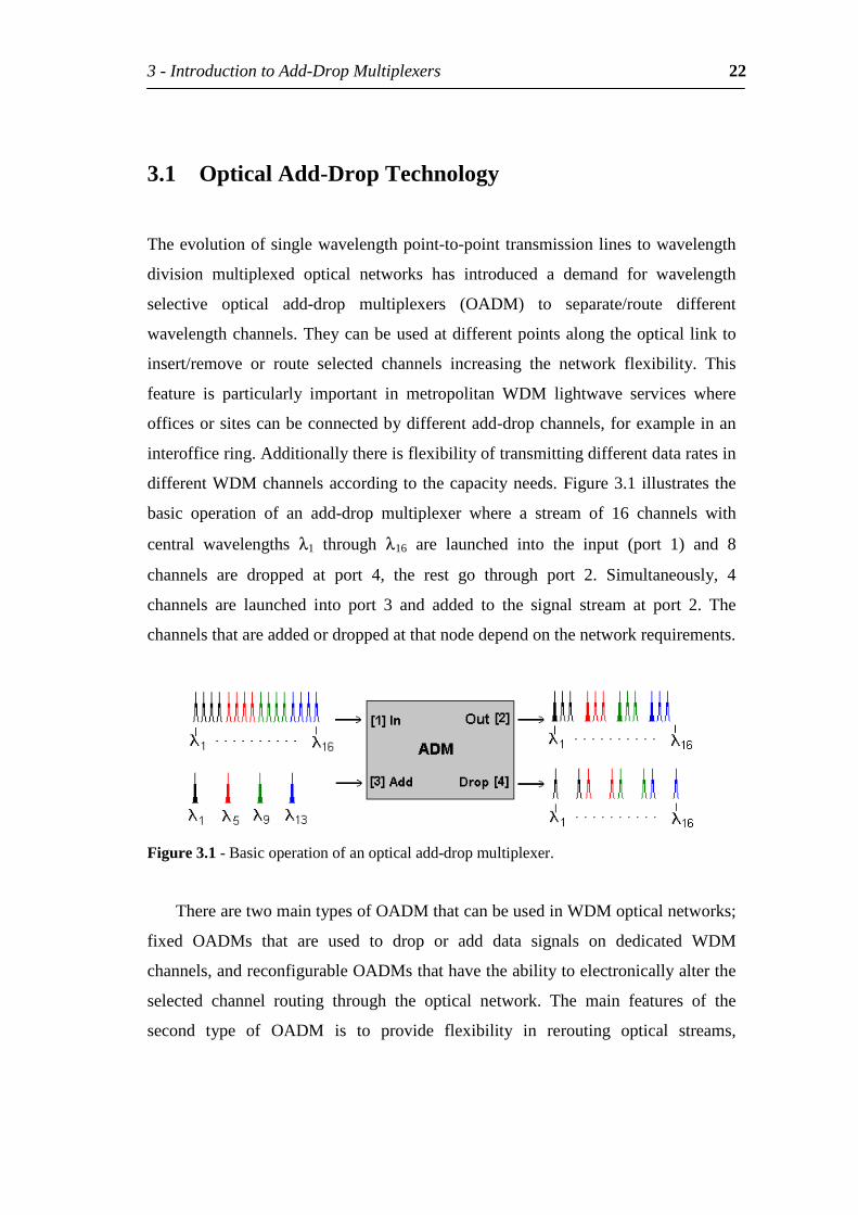
differentWDMchannelsaccordingtothecapacityneeds.Figure3.1illustrates the
basic operation of an add-drop multiplexer where a stream of 16 channels with
central wavelengths λ1 through λ16 are launched into the input (port 1) and 8
channels are dropped at port 4, the rest go through port 2. Simultaneously, 4
channels are launched into port 3 and added to the signal stream at port 2. The
channelsthatareaddedordroppedatthatnodedependonthenetworkrequirements.
Figure3.1-Basicoperationofanopticaladd-dropmultiplexer.
TherearetwomaintypesofOADMthatcanbeusedinWDMopticalnetworks;
fixed OADMs that are used to drop or add data signals on dedicated WDM
channels,andreconfigurableOADMsthathavetheabilitytoelectronicallyalterthe
selected channel routing through the optical network. The main features of the
second type of OADM is to provide flexibility in rerouting optical streams,
3-IntroductiontoAdd-DropMultiplexers 23
bypassingfaultyconnections,allowingminimalservicedisruptionandtheabilityto
adaptorupgradetheopticalnetworktodifferentWDMtechnologies.
Configurations presented in the literature to perform the required add or drop
functions use both planar and fibre technology. Planar devices [28-36] provide
compact solutionswith thepossibilityofaddingordroppingmanychannelsusing
onlyoneintegratedopticalcircuitusingarrayed-waveguide-grating(AWG)[34]or-
waveguide-grating-router (WGR) technology [35, 36]. The main drawbacks of
planardevicesaretheirhighinsertionloss,whichcanbeashighas7dB,andtheir
polarisation dependence. Alternatively, all-fibre devices [37-47] are attractive
solutionsdue to their low insertion losses,polarisation insensitivity (dependingon
thefibreandconfiguration)andeaseofcouplingbetweendeviceoutputandinputs
oftheopticalnetworkusingsimplesplicesandpigtails.Typically,duetotheirlarger
dimensionsthesedevicesaresensitivetoenvironmentalvariations,dependentupon
the configuration.Devicesbased in free spaceoptics (micromirrors andgratings)
have also been used successfully to perform add-drop operations with good
performance[48].Although,thesedevicesareingeneralmoreexpensiveandhave
relatively high insertion losses. Finally thin film filter devices have been
traditionally used for multiplexing/demultiplexers purposes. Fibre and planar add-
dropconfigurationsandtheirrespectiveperformancearediscussedinthefollowing
section.
3.2 Add-DropConfigurations
Excellent performance and compactness offered by four-port planar-waveguide-
based devices can be rivalled by the simple all-fibre add-drop configuration, as
showninFigure3.2.Itconsistsofa3dBsplitterandagratinginoneoftheoutput
arms; light launched into port1 is split in two, λG is reflected by the grating then
droppedatPort4.Theothercoupleroutputportisimmersedinanindexmatching
fluidsothatthelightisnotreflected.Theselectedsignalemergesatboththeinput
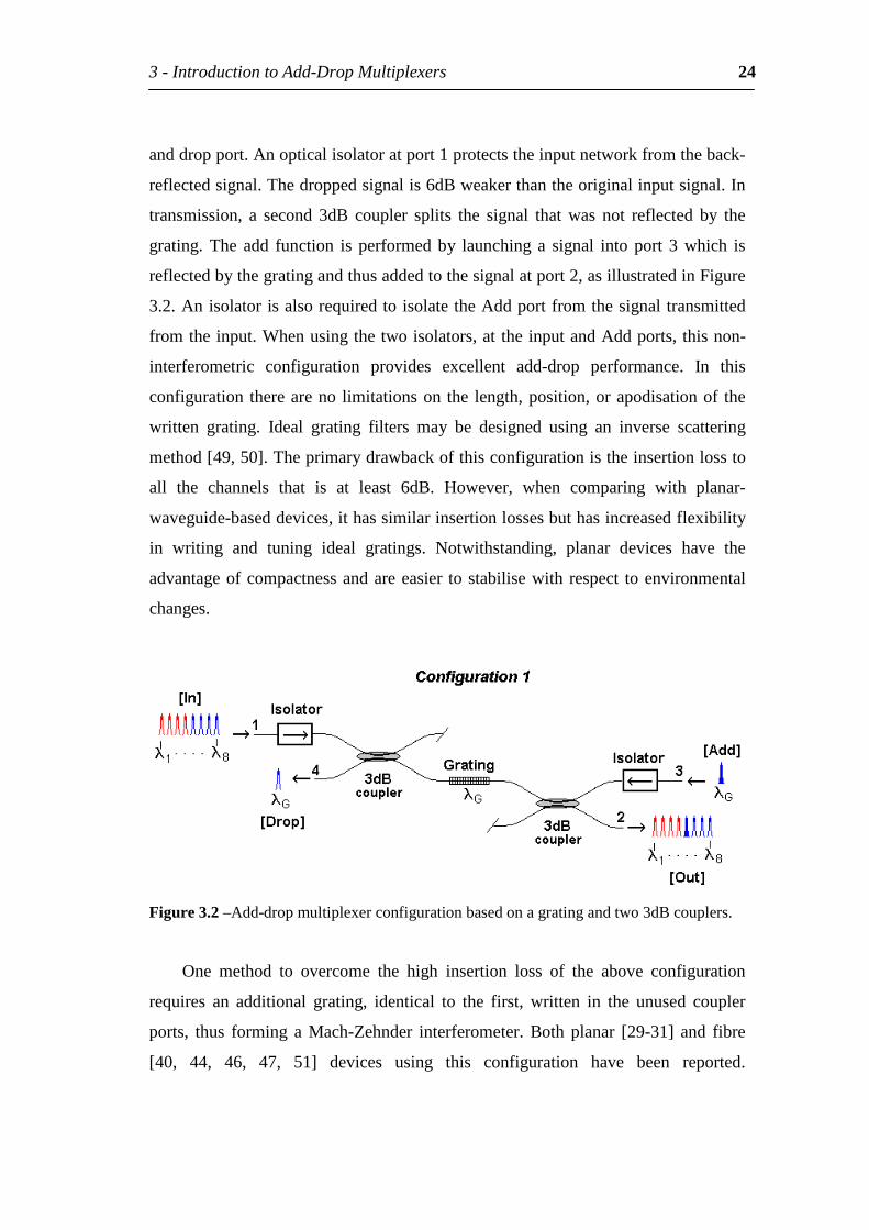
3-IntroductiontoAdd-DropMultiplexers 24
anddropport.Anopticalisolatoratport1protectstheinputnetworkfromtheback-
reflectedsignal.Thedroppedsignalis6dBweakerthantheoriginalinputsignal.In
transmission, a second 3dB coupler splits the signal that was not reflected by the
grating.The add function isperformedby launchinga signal intoport 3which is
reflectedbythegratingandthusaddedtothesignalatport2,asillustratedinFigure
3.2.Anisolator isalsorequiredtoisolatetheAddportfromthesignaltransmitted
fromtheinput.Whenusingthetwoisolators,at theinputandAddports,thisnon-
interferometric configuration provides excellent add-drop performance. In this
configuration thereareno limitationsonthe length,position,orapodisationof the
written grating. Ideal grating filters may be designed using an inverse scattering
method[49,50].Theprimarydrawbackofthisconfigurationistheinsertionlossto
all the channels that is at least 6dB. However, when comparing with planar-
waveguide-baseddevices,ithassimilarinsertionlossesbuthasincreasedflexibility
in writing and tuning ideal gratings. Notwithstanding, planar devices have the
advantageofcompactnessandareeasier tostabilisewithrespect toenvironmental
changes.
Figure3.2–Add-dropmultiplexerconfigurationbasedonagratingandtwo3dBcouplers.
One method to overcome the high insertion loss of the above configuration
requires an additional grating, identical to the first, written in the unused coupler
ports, thus forming a Mach-Zehnder interferometer. Both planar [29-31] and fibre
[40, 44, 46, 47, 51] devices using this configuration have been reported.
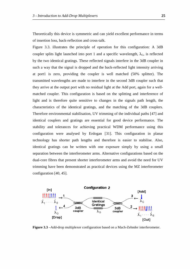
3-IntroductiontoAdd-DropMultiplexers 25
Theoreticallythisdeviceissymmetricandcanyieldexcellentperformanceinterms
ofinsertionloss,back-reflectionandcross-talk.
Figure 3.3. illustrates the principle of operation for this configuration: A 3dB
couplersplits light launched intoport1andaspecificwavelength,λG, is reflected
bythetwoidenticalgratings.Thesereflectedsignalsinterfereinthe3dBcouplerin
suchawaythatthesignalisdroppedandtheback-reflectedlightintensityarriving
at port1 is zero, providing the coupler is well matched (50% splitter). The
transmittedwavelengthsaremade to interfere in thesecond3dBcoupler such that
theyarriveattheoutputportwithnoresiduallightattheAddport,againforawell-
matched coupler. This configuration is based on the splitting and interference of
light and is therefore quite sensitive to changes in the signals path length, the
characteristics of the identical gratings, and the matching of the 3dB couplers.
Thereforeenvironmentalstabilisation,UVtrimmingoftheindividualpaths[47]and
identical couplers and gratings are essential for good device performance. The
stability and tolerances for achieving practical WDM performance using this
configuration were analysed by Erdogan [31]. This configuration in planar
technology has shorter path lengths and therefore is easier to stabilise. Also,
identical gratings can be written with one exposure simply by using a small
separationbetweentheinterferometerarms.Alternativeconfigurationsbasedonthe
dual-corefibresthatpresentshorterinterferometerarmsandavoidtheneedforUV
trimminghavebeendemonstratedaspracticaldevicesusingtheMZinterferometer
configuration[40,45].
Figure3.3–Add-dropmultiplexerconfigurationbasedonaMach-Zehnderinterferometer.
3-IntroductiontoAdd-DropMultiplexers 26
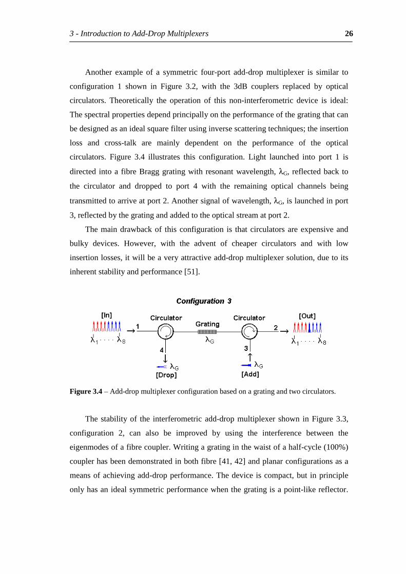
Another example of a symmetric four-port add-drop multiplexer is similar to
configuration 1 shown in Figure 3.2, with the 3dB couplers replaced by optical
circulators. Theoretically the operation of this non-interferometric device is ideal:
Thespectralpropertiesdependprincipallyontheperformanceofthegratingthatcan
bedesignedasanidealsquarefilterusinginversescatteringtechniques;theinsertion
loss and cross-talk are mainly dependent on the performance of the optical
circulators. Figure 3.4 illustrates this configuration. Light launched into port 1 is
directed intoa fibreBragggratingwithresonantwavelength,λG, reflectedback to
the circulator and dropped to port 4 with the remaining optical channels being
transmittedtoarriveatport2.Anothersignalofwavelength,λG,islaunchedinport
3,reflectedbythegratingandaddedtotheopticalstreamatport2.
Themaindrawbackof thisconfiguration is thatcirculators are expensiveand
bulky devices. However, with the advent of cheaper circulators and with low
insertionlosses,itwillbeaveryattractiveadd-dropmultiplexersolution,duetoits
inherentstabilityandperformance[51].
Figure3.4–Add-dropmultiplexerconfigurationbasedonagratingandtwocirculators.
Thestabilityof the interferometric add-dropmultiplexer shown inFigure3.3,
configuration 2, can also be improved by using the interference between the
eigenmodesofafibrecoupler.Writingagratinginthewaistofahalf-cycle(100%)
couplerhasbeendemonstratedinbothfibre[41,42]andplanarconfigurationsasa
meansofachievingadd-dropperformance.Thedeviceiscompact,but inprinciple
onlyhasanidealsymmetricperformancewhenthegratingisapoint-likereflector.
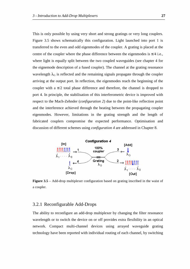
3-IntroductiontoAdd-DropMultiplexers 27
Thisisonlypossiblebyusingveryshortandstronggratingsorverylongcouplers.
Figure 3.5 shows schematically this configuration. Light launched into port 1 is
transferredtotheevenandoddeigenmodesofthecoupler.Agratingisplacedatthe
centreofthecouplerwherethephasedifferencebetweentheeigenmodesisπ/4i.e.,
wherelightisequallysplitbetweenthetwocoupledwaveguides(seechapter4for
theeignemodedescriptionofafusedcoupler).Thechannelatthegratingresonance
wavelengthλGisreflectedandtheremainingsignalspropagatethroughthecoupler
arrivingattheoutputport.Inreflection,theeigenmodesreachthebeginningofthe
coupler with a π/2 total phase difference and therefore, the channel is dropped to
port4.Inprinciple,thestabilisationofthisinterferometricdeviceisimprovedwith
respecttotheMach-Zehnder(configuration2)duetothepoint-likereflectionpoint
andtheinterferenceachievedthroughthebeatingbetweenthepropagatingcoupler
eigenmodes. However, limitations in the grating strength and the length of
fabricated couplers compromise the expected performance. Optimisation and
discussionofdifferentschemesusingconfiguration4areaddressedinChapter8.
Figure3.5–Add-dropmultiplexerconfigurationbasedongratinginscribedinthewaistof
acoupler.
3.2.1 ReconfigurableAdd-Drops
Theabilitytoreconfigureanadd-dropmultiplexerbychangingthefilterresonance
wavelengthortoswitchthedeviceonoroffprovidesextraflexibilityinanoptical
network. Compact multi-channel devices using arrayed waveguide grating
technologyhavebeenreportedwithindividualroutingofeachchannel,byswitching
3-IntroductiontoAdd-DropMultiplexers 28
itonoroff[32,34].Eventhoughlowcross-talkisachievablewithmultiplepasses
throughthemultiplexer,thesedeviceshaveunavoidablyhighinsertionlosses.
On theotherhand,all-fibreadd-dropconfigurationshavepotentiallyno cross
talk (dependingon the filter design)withvery low insertion loss.Whenusing the
non-interferometric add-drop configurations 1 or 3, wavelength selection is
achievable by straining [52] or heating [53] the Bragg grating. Whilst using the
interferometric configuration 2, both fibre gratings should be affected equally and
therefore wavelength tuning is not practicable. However, switching is possible by
unbalancingtheinterferometerbystrainingorheatingonlyoneofthearms.
3.3 Add-DropPerformance
The analogue performance of add-drop multiplexers is characterised by using
scatteringparametersSij foreachpairofports [54].Thefirstsubscript, i, refers to
the destination port and the second subscript, j, the input port. Several properties
may be characterised using the scattering parameter namely; the insertion loss,
polarisation dependent loss (PDL), dropped channel isolation, channel uniformity,
frequencyaccuracyandbandwidthconsiderations.InappendixAsystemapplication
characteristicsfortheisolationoftheopticalportsachievablewithcurrent50,100,
200 and 400 GHz channel-spacing technologies as well as, cross-talk, back-
reflectionand insertion loss requirementsaregiven.The remainingparametersare
definedtoin[54].
3.3.1 IsolationandCrosstalk
The two main parameters related to the isolation of channels in an add-drop
multiplexerarethethrough-portisolationofadroppedchannel(S21parameter)and
thedrop-portisolationofthroughchannels(S43parameter).Notethatinasymmetric
device S43=S21. These two parameters represent the sources of the interchannel
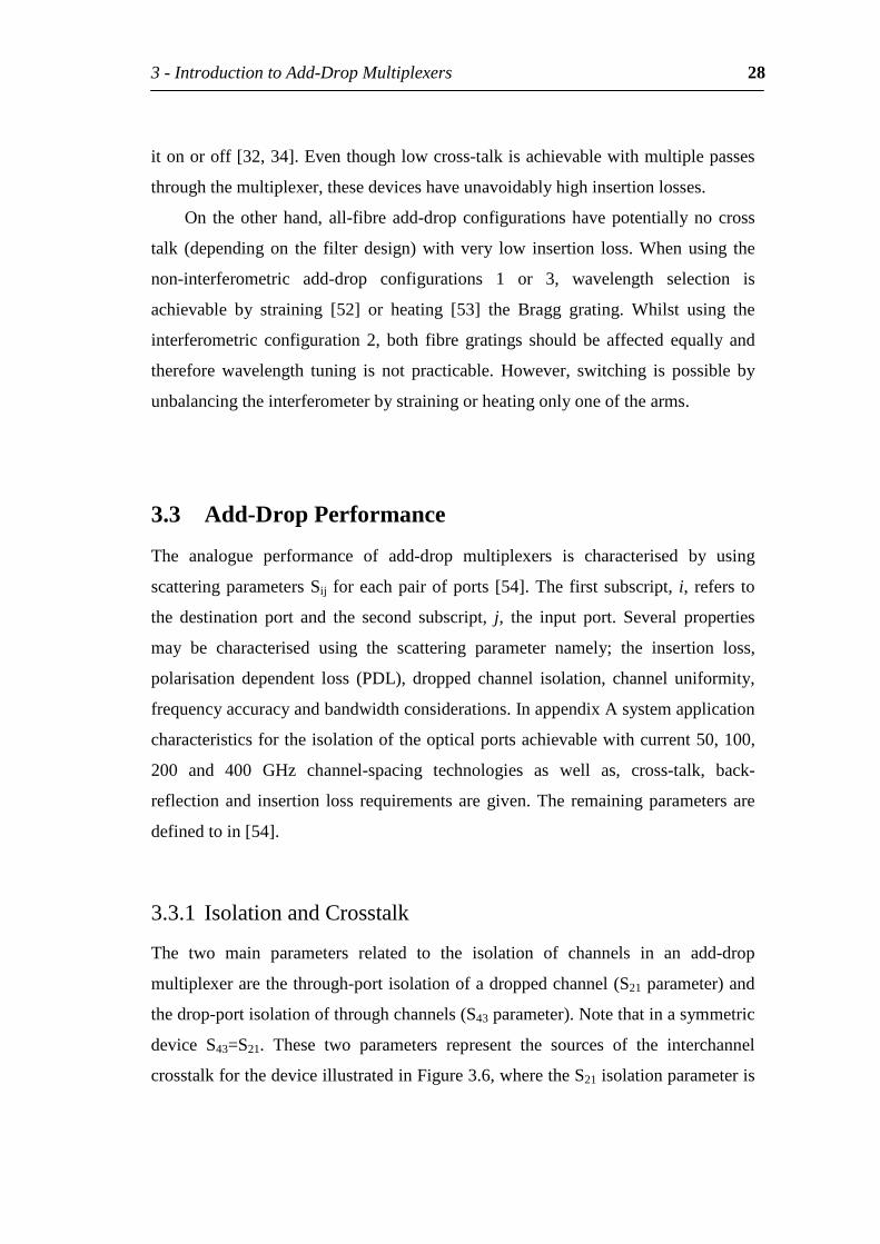
crosstalkforthedeviceillustratedinFigure3.6,wheretheS21isolationparameteris
3-IntroductiontoAdd-DropMultiplexers 29
highlighted.Iftheamountofpowerlaunchedintoport1,P1,andthedroppedpower
toport4,P4,theremainingtransmittedpower,P2,emergesatport2asinterchannel
crosstalk.Themeasureofisolationisgivenby-10log(P1/P2).
Figure3.6–ExampleoftheS21isolationofthethroughportofadroppedchannel.
The second kind of crosstalk is due to unwanted signals transferred from
neighbouringchannelstothefilteredone,andisnamedintrachannelcrosstalk[55].
Itcanappearintheinterferometricconfigurationsasaresultofanincorrectsplitting
ratio in the 3dB (50%-50%) couplers. This kind of crosstalk however, has a low
powerpenaltyintheperformanceoftheWDMsystem.
3.3.2 Insertionlosses
Insertion lossesare theattenuation in theopticalpowerof thechannelsdue to the
insertion of the device. The effect of the device insertion loss is schematically
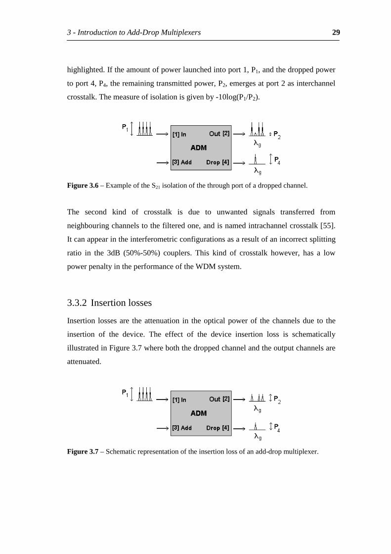
illustratedinFigure3.7whereboththedroppedchannelandtheoutputchannelsare
attenuated.
Figure3.7–Schematicrepresentationoftheinsertionlossofanadd-dropmultiplexer.
3-IntroductiontoAdd-DropMultiplexers 30
Theinsertionloss,linscorrespondingtothetransferefficiencyoflightfromportito
portjaffectsallthechannelsequallyandisdescribedby
=
j
iins P
Pl log10
PiandPjarethepowersofagivensignalchannelattherespectiveportsassuming
thereisnocross-talkorpolarisation-dependentloss(PDL).
3.3.3 Back-reflections
Back-reflectionsaredefinedbythescatteringparametersSii.Thesubscriptiis1or3
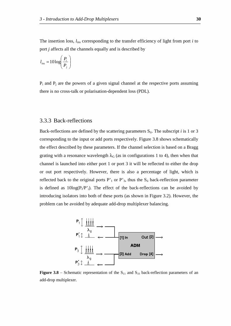
correspondingtotheinputoraddportsrespectively.Figure3.8showsschematically
theeffectdescribedbytheseparameters.IfthechannelselectionisbasedonaBragg
gratingwitharesonancewavelengthλG(asinconfigurations1to4),thenwhenthat
channelislaunchedintoeitherport1orport3itwillbereflectedtoeitherthedrop
or out port respectively. However, there is also a percentage of light, which is
reflectedbacktotheoriginalportsP’ 1orP’ 3,thustheSiiback-reflectionparameter
is defined as 10log(Pi/P’ i). The effect of the back-reflections can be avoided by
introducingisolatorsintobothoftheseports(asshowninFigure3.2).However,the
problemcanbeavoidedbyadequateadd-dropmultiplexerbalancing.
Figure3.8–Schematicrepresentationof theS11andS33back-reflectionparametersofan
add-dropmultiplexer.
3-IntroductiontoAdd-DropMultiplexers 31
3.4 Summary
Add-dropmultiplexersaredevicesinhighdemandcompatiblewithbothLANand
longhaulnetworks.DuetothenumberofnodesusedinLANs,andthusthenumber
add-dropmultiplexersrequired,demandforcheapdevicesistheprimarymotivation.
All-fibreadd-dropmultiplexerconfigurationsarepotentialcandidatesforproviding
suchcheapdevices.Thedifferentschemeswillbefurtheraddressedinchapter8.In
summary, this chapter was a review of the existing technologies for routing
wavelength channels,withdiscussion regarding the advantages anddrawbacks for
each. Parameters, which are used to characterise the performance of add-drop
multiplexers, were also introduced. This chapter provides OADM fundamentals
relevant to section III, where the optimisation of three different all-fibre add-drop
multiplexerschemesisdiscussed.
4
IntroductiontoFibre-
Couplers
Theaimofthischapteristoprovideanoverviewoffibrecouplertechnology.The
principles of how fibre couplers exchange power between the two ports are
presented and different methods of fabrication are compared. The information
providedinthischapterintroducestheworkonthecharacterisationoffibrecouplers
(Chapter 9) and is relevant to the optimisation of all-fibre add-drop multiplexers
basedontheinscriptionofgratingsinthecouplerwaist(Chapter8).
4-IntroductiontoFibre-Couplers 33
4.1 CouplerTechnology
Fibre- and integrated-optic couplers are extremely important components in a
number of photonics applications. They are generally four-port devices and their
operation relieson thedistributed couplingbetween two individualwaveguides in
closeproximity,whichresultsinagradualpowertransferbetweenmodessupported
bythetwowaveguides.Thispowertransferandcross-couplingatthecoupleroutput
ports can be viewed also, as a result of the beating between eigenmodes of the
compositetwo-waveguidestructurealongthelengthofthecompositecouplerwaist
[56]. The most common use of fibre- and integrated-optic couplers is as a power
splitter, this is, the fibre-optic equivalentof a free spaceopticbeam-splitter.They
canbeusedtosplittheopticalpowerofanopticalchannel(ofcertainwavelength)
betweentheoutputports[57].Anotherapplicationistocombineorsplitthepower
ofdifferentchannels,correspondingtodifferentwavelengths(wavelength-division-
multiplexing (WDM) splitters/combiners) [58]. Lately fibre- and integrated-optic
couplers,havebeencombinedwithreflectiveBragggratingswrittenintheirwaist,
toprovideselectiveaddinganddroppingofdifferentchannelsinWDMsystems[41,
42].
4.2 TheoreticalCouplerDescription
A fibrecoupler isa four-portdeviceconsistingof two fibres thathavebeen fused
together, etched, or polished over a small interaction region. The mechanism
through which light is exchanged between the two fibres is dependent upon the
fabricationmethod.Whenthefibresareetchedorpolishedandpositionedinclose
proximity, the otherwise insensitive and well confined core modes interact by
exchangingpowerbetweeneach fibre coredue to theoverlapof themodes in the
commoncladding.Thestrengthofthecouplingbetweenthetwomodesisdescribed
4-IntroductiontoFibre-Couplers 34
by an overlap integral of the fields associated with each of the individual guides.
Fusedcouplersareobtainedbyfusingtogetherandstretchingtwoparalleluncoated
fibres. As the fibres are stretched the core sizes decrease until the modes (at the
wavelength of interest) are no longer guided by the core but by the composite
cladding-airstructure.Ifthetaperisadiabaticonlythetwolowest-ordereigenmodes
of this structure will be excited and the power exchange is due to the beating
betweenthesetwoeigenmodes.Intheworkpresentedhereonlyfusedfibrecouplers
arediscussed.
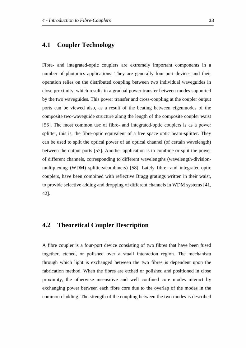
Figure 4.1 - Four-port coupler schematic showing the coupling region (LC), which is
comprisedoftwotaperregions(LT1,LT2)andthecouplerwaist(LW).
Consider the 2x2 coupler shown schematically in Figure 4.1. When light is
launchedintoport1,thenormalisedfieldamplitudesoftheeven(Ae)andodd(Ao)
eigenmodesatthecouplerinput(z=0)canbeapproximatedby[56]:
2
)0()0()0(;
2)0()0(
)0( 2121 AAA
AAA oe
−=+= (4.1)
whereA1(0)andA2(0)arethenormalisedamplitudesofthefieldslaunchedintothe
twoinputports1and2,respectively.Forsingleportexcitation,A1(0)=1andA2(0)=0
and,throughEquation(4.1),Ae(0)=Ao(0)=1/ 2 .Therefore,lightlaunchedintoone
of the inputportsofa2x2couplerexcitesequally the two lowest-order (evenand
odd) eigenmodes along the coupling region. The two eigenmodes propagate
adiabaticallyalong theentirecouplingregionwithpropagationconstantsβe(z)and
βo(z)respectively.Thebeatingbetweenthesetwomodesthenprovidesthecoupling
ofpoweralongthecoupler.
4-IntroductiontoFibre-Couplers 35
Even
+ + +
Odd
∆φeo 0 3π/2 2π
P1
P1
P2
P2
ππ/2
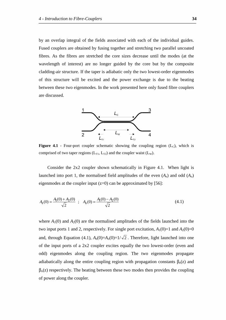
Figure4.2-Schematicofevenandoddeigenmodebeatingandtotalpowerevolutionalong
a2x2full-cycle(∆φeo=2π)coupler.
Thepropagatingtotalelectricfieldatanypointalongthecouplerisdescribedby:
+
=+=
−−z
o
z
e di
o
di
eoet ezAezAzEzEzE 00
)()(
)()()()()(ζζβζζβ
(4.2)
During adiabatic propagation, the even and odd eigenmodes retain their
amplitude(Ae(z)=Ae(0)andAo(z)=Ao(0))andchangeonlytheirrelativephase.This
results inspatialbeatingalong thecouplerwaistandpowerredistributionbetween
the two individual waveguides comprising the optical coupler. The peak field
amplitudes for each individual waveguide, along the coupling region, can be
approximatedby[56]:
4-IntroductiontoFibre-Couplers 36
[ ]
[ ]
−=−=
=+=
+−
+−
z
oe
z
oe
dioe
dioe
ezizEzE
zE
ezzEzE
zE
0
0
)()(21
2
)()(21
1
)(21
sin2
)()()(
)(21
cos2
)()()(
ζζβζβ
ζζβζβ
φ
φ
(4.3)
where [ ] −=∆==z
oe
z
eoeo ddzz00
)()()()()( ζζβζβζζβφφ is the relative
accumulatedphasedifferencebetweentheevenandoddeigenmodes.βeandβoare
the propagation constants of the even and odd eigenmodes, respectively. The
correspondingnormalisedpeakpowercarriedbytheindividualwaveguidesisgiven
byP1(2)=|E1(2)|2,namely
=
=
)(21
sin)(
)(21
cos)(
22
21
zzP
zzP
φ
φ (4.4)
At thepointsalong thecoupler,whereφ iszerooramultipleof2π, the total
powerisconcentratedpredominantlyaroundwaveguide#1(P1=1andP2=0).Atthe
pointsalongthecoupler,whereφismultipleofπ,ontheotherhand,thetotalpower
isconcentratedpredominantlyaroundwaveguide#2(P1=0andP2=1).Finally,atthe
pointswhereφ ismultipleofπ/2, the totalpower isequallysplitbetween the two
waveguides (P1=P2). The even/odd eigenmode beating and total power evolution
alongafull-cyclecoupler(φ=2π)isshownschematicallyinFigure4.2.Thecoupling
coefficient k(z) describing the strength of the interaction between the eigenmodes
andisgivenby:
2)()(
)(zz
zk oe ββ −= (4.5)
4-IntroductiontoFibre-Couplers 37
The coupler beat length LB is defined as the minimum interaction length the two
eigenmodes,initiallyinphase,musttravelinordertointerfereconstructivelyi.e.,to
beagaininphase:
oeBL
ββπ−
= 2 (4.6)
4.3 FabricationofFusedFibreCouplers
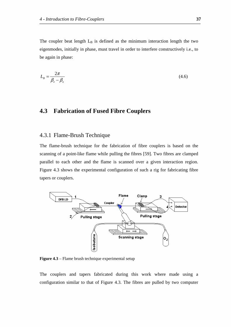
4.3.1 Flame-BrushTechnique
The flame-brush technique for the fabrication of fibre couplers is based on the
scanningofapoint-likeflamewhilepullingthefibres[59].Twofibresareclamped
parallel to each other and the flame is scanned over a given interaction region.
Figure4.3shows theexperimentalconfigurationofsucha rig for fabricatingfibre
tapersorcouplers.
Figure4.3–Flamebrushtechniqueexperimentalsetup
The couplers and tapers fabricated during this work where made using a
configuration similar to thatofFigure4.3.The fibres arepulledby two computer
4-IntroductiontoFibre-Couplers 38
controlledAerotechstages.TheflameisscannedusingathirdAerotechstage.The
flame gas consists of a mixture of isobutene and oxygen. Both cleaning and
alignmentofthefibresiscrucialforfabricatinguniformtapersorcouplerswithlow
insertion losses. Air draughts or gas pressure variations can severely affect the
quality of the devices, due to variations in the flame temperature and consequent
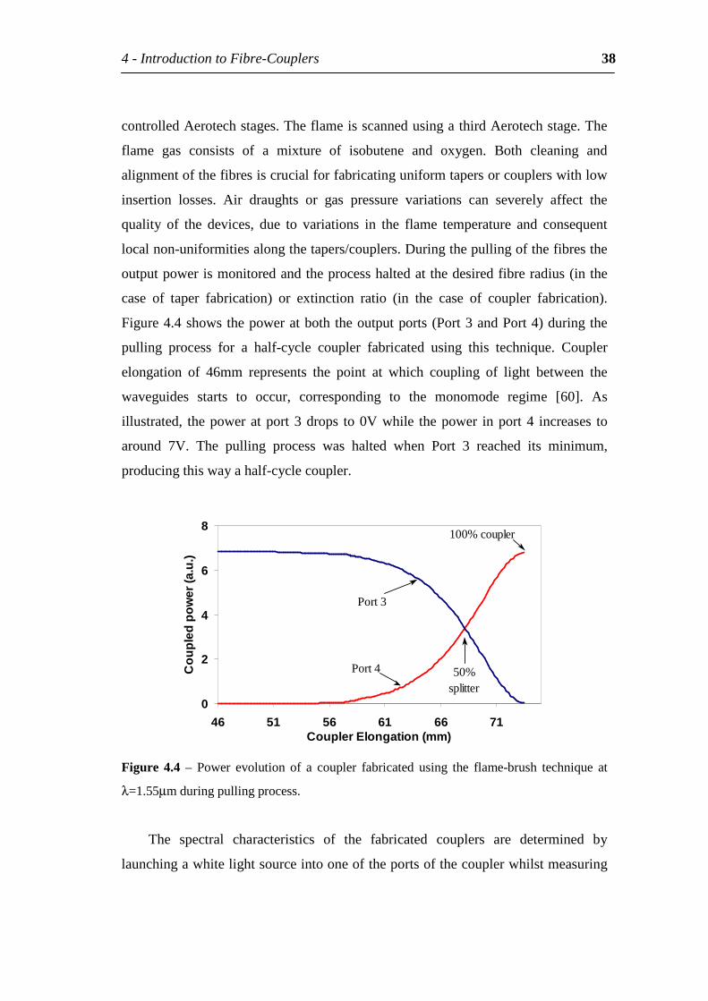
localnon-uniformitiesalongthetapers/couplers.Duringthepullingofthefibresthe
outputpowerismonitoredandtheprocesshaltedatthedesiredfibreradius(inthe
case of taper fabrication) or extinction ratio (in the case of coupler fabrication).
Figure4.4showsthepoweratboththeoutputports(Port3andPort4)duringthe
pulling process for a half-cycle coupler fabricated using this technique. Coupler
elongation of 46mm represents the point at which coupling of light between the
waveguides starts to occur, corresponding to the monomode regime [60]. As
illustrated, thepoweratport3drops to0Vwhile thepower inport4 increases to
around 7V. The pulling process was halted when Port 3 reached its minimum,
producingthiswayahalf-cyclecoupler.
0
2
4
6
8
46 51 56 61 66 71CouplerElongation(mm)
Cou
pled
pow
er(a
.u.)
Port4
Port3
50%splitter
100%coupler
Figure 4.4 – Power evolution of a coupler fabricated using the flame-brush technique at
λ=1.55µmduringpullingprocess.
The spectral characteristics of the fabricated couplers are determined by
launchingawhitelightsourceintooneoftheportsofthecouplerwhilstmeasuring
4-IntroductiontoFibre-Couplers 39
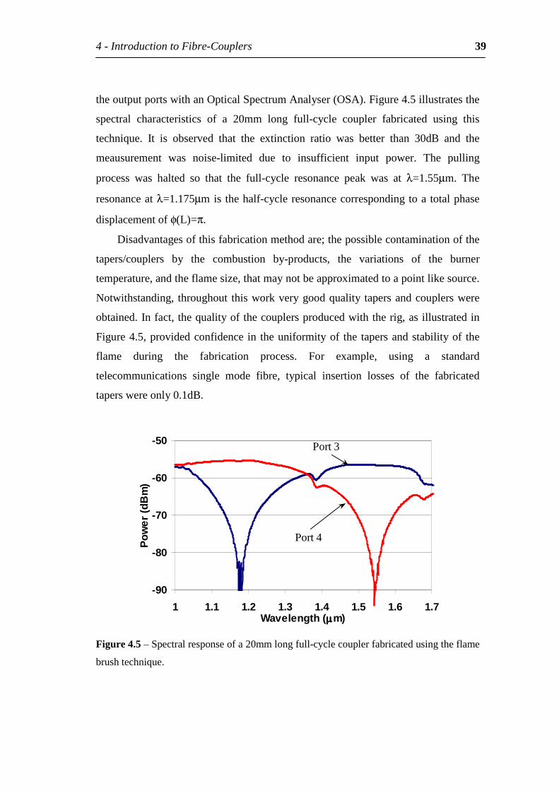
theoutputportswithanOpticalSpectrumAnalyser(OSA).Figure4.5illustratesthe
spectral characteristics of a 20mm long full-cycle coupler fabricated using this
technique. It is observed that the extinction ratio was better than 30dB and the
meausurement was noise-limited due to insufficient input power. The pulling
process was halted so that the full-cycle resonance peak was at λ=1.55µm. The
resonanceatλ=1.175µmis thehalf-cycleresonancecorrespondingtoa totalphase
displacementofφ(L)=π.
Disadvantagesofthisfabricationmethodare;thepossiblecontaminationofthe
tapers/couplers by the combustion by-products, the variations of the burner
temperature,andtheflamesize,thatmaynotbeapproximatedtoapointlikesource.
Notwithstanding, throughout thisworkverygoodquality tapersandcouplerswere
obtained.Infact,thequalityofthecouplersproducedwiththerig,asillustratedin
Figure4.5,providedconfidence in theuniformityof the tapersandstabilityof the
flame during the fabrication process. For example, using a standard
telecommunications single mode fibre, typical insertion losses of the fabricated
taperswereonly0.1dB.
-90
-80
-70
-60
-50
1 1.1 1.2 1.3 1.4 1.5 1.6 1.7Wavelength(µµµµm)
Pow
er(d
Bm
)
Port3
Port4
Figure4.5–Spectralresponseofa20mmlongfull-cyclecouplerfabricatedusingtheflame
brushtechnique.
4-IntroductiontoFibre-Couplers 40
4.3.2 CO2Laser
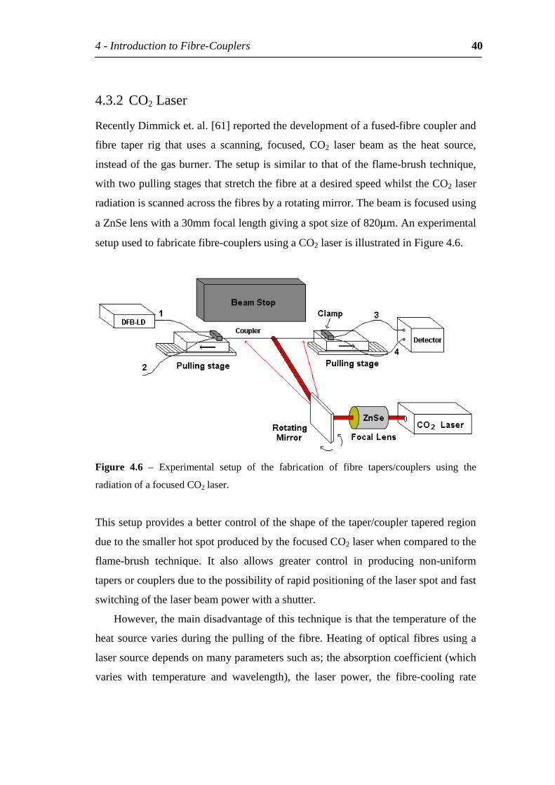
RecentlyDimmicket.al.[61]reportedthedevelopmentofafused-fibrecouplerand
fibre taper rig that uses a scanning, focused, CO2 laser beam as the heat source,
insteadofthegasburner.Thesetupissimilartothatoftheflame-brushtechnique,
withtwopullingstagesthatstretchthefibreatadesiredspeedwhilsttheCO2laser
radiationisscannedacrossthefibresbyarotatingmirror.Thebeamisfocusedusing
aZnSelenswitha30mmfocallengthgivingaspotsizeof820µm.Anexperimental
setupusedtofabricatefibre-couplersusingaCO2laserisillustratedinFigure4.6.
Figure 4.6 – Experimental setup of the fabrication of fibre tapers/couplers using the
radiationofafocusedCO2laser.
Thissetupprovidesabettercontroloftheshapeofthetaper/couplertaperedregion
duetothesmallerhotspotproducedbythefocusedCO2laserwhencomparedtothe
flame-brush technique. It also allows greater control in producing non-uniform
tapersorcouplersduetothepossibilityofrapidpositioningofthelaserspotandfast
switchingofthelaserbeampowerwithashutter.
However,themaindisadvantageofthistechniqueisthatthetemperatureofthe
heatsourcevariesduring thepullingof thefibre.Heatingofoptical fibresusinga
lasersourcedependsonmanyparameterssuchas;theabsorptioncoefficient(which
varies with temperature and wavelength), the laser power, the fibre-cooling rate
4-IntroductiontoFibre-Couplers 41
(which depends on the fibre radius and temperature), and the laser spot size. To
overcome this problem the laser power has to be adjusted constantly in order to
maintainaconstant temperatureduring thefibrepulling. Incontrast,whenheating
with a flame burner, the presence or not of the fibre has little or no effect on the
temperatureoftheheatsourceduetothemechanismofheatgeneration.
4.3.3 HeatingOven
Anothertechniqueusedinindustryforfabricatingfibrecouplersandtapersrelieson
heatingthewholeuniformsectionusinganovenorresistiveelectricalheaterwhile
pullingthefibres.Duetothelongheatzonethistechniquehasnocontroloverthe
shape of the tapered region although the sensitivity to environmental factors is
reduced. The quality of the tapers/couplers is essentially dependent on the oven
design,andthetemperatureuniformityalongthelengthofwaistregion.
4.3.4 ShapeoftheTaperedRegion
Accuratecontrolofthetaperedregionshapeofbothfibrecouplersandfibretapers
canbecrucialfortheperformanceofdevicesusingthesecomponents.Forexample,
inchapter5anAOtunablefilterisdiscussed,whichreliesontheaccuratecontrolof
thefibre-tapershapeandlength.Birksetal.[62],usingtheflame-brushtechnique,
produceda longuniformtaperwaist (90mm)withshort transitionregions(35mm)
and very small waist diameters (~2µm), for generating a supercontinuum light
spectrum. Also in fibre couplers, the accurate control of the tapered region is
extremelyimportantforthefabricationofnon-uniformcouplersthatcanbeusedas
an add-drop multiplexer when a grating is inscribed in the waist (chapter 8). In
general, the transition region for both fibre couplers and tapers should obey the
adiabaticcriterion[63],inordertominimiseinsertionlosses.
4-IntroductiontoFibre-Couplers 42
The shape of fibre tapers/couplers produced by using scanning point-like
heatingsourceshasbeenextensivelystudiedbyBirkselal.[64].Assumingthatthe
localisedheatingofthefibremakestheglasssoftenoughtobestretchedwhilstnot
being so soft that it falls under its own weight, the shape of the tapers can be
calculated without having to recur to fluid mechanics beyond the principle of
conservation of mass. A tapered fibre, at any given time (or elongation) of the
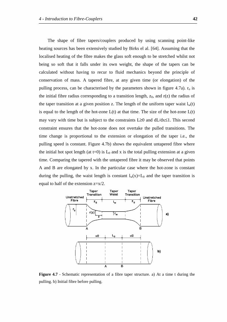
pullingprocess,canbecharacterisedbytheparametersshowninfigure4.7a).ro is
theinitialfibreradiuscorrespondingtoatransitionlength,z0,andr(z)theradiusof
thetapertransitionatagivenpositionz.Thelengthoftheuniformtaperwaistlw(t)
isequaltothelengthofthehot-zoneL(t)atthattime.Thesizeofthehot-zoneL(t)
mayvarywithtimebutissubjecttotheconstraintsL≥0anddL/dx≤1.Thissecond
constraint ensures that the hot-zone does not overtake the pulled transitions. The
time change is proportional to the extension or elongation of the taper i.e., the
pullingspeed isconstant.Figure4.7b)shows theequivalentuntaperedfibrewhere
theinitialhotspotlength(att=0)isL0andxisthetotalpullingextensionatagiven
time.Comparingthetaperedwiththeuntaperedfibreitmaybeobservedthatpoints
AandB are elongated byx. In theparticular casewhere thehot-zone is constant
during thepulling, thewaist length isconstant lw(x)=L0 and the taper transition is
equaltohalfoftheextensionz=x/2.
Figure4.7 -Schematic representationofa fibre taper structure.a)Ata time tduring the
pulling.b)Initialfibrebeforepulling.
4-IntroductiontoFibre-Couplers 43
From the conservation of mass principle, the following expression can easily be
derived:
Lr
dxdr ww
2−= (4.7)
Secondly, the extension x can be related to the taper transition length z by
comparingtheinitiallengthABatt=0,withthetotaltaperlengthABatanygiven
time:
02 LxLz +=+ (4.8)
The particular case where the hot-zone remains constant during the fibre
extensionhasbeenanalysedby[64-66].InthiscaseL(z)=L0andz=x/2.Integrating
(4.7)givesthewaistshapeforatotalfibreextensionx.
( )00 20
)'('
2/1
0)( LxxLdx
w ererxr
x
−
−
=
= (4.9)
The taper profile is calculated by substituting x=2z in (4.9), resulting in the well-
knownexponentialdecayprofile.Allthetaperandcouplerdevicesdiscussedinthis
thesiswerefabricatedusingaconstanthot-zone,thusexpression(4.9)issufficientto
describe the profiles of the tapered regions. Further examples of interest are
discussedin[64]whereequation(4.7)isdemonstratedaswell.
Inorder tominimizelossesbetweenthefundamentalandthenearestcladding
modes,thetaperangle|dr/dz|hastoobeytheadiabaticcriterion[63].
( ) ( )( )π
ββ2
21 zzrdzdr −≤ (4.10)
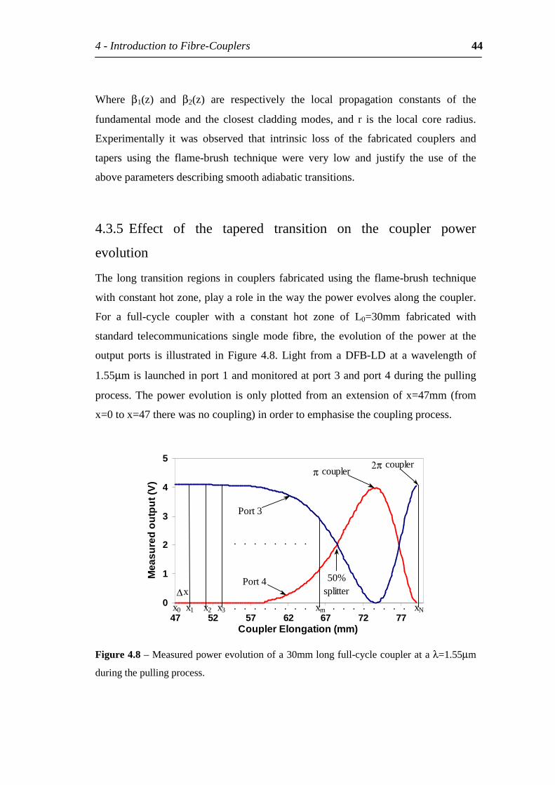
4-IntroductiontoFibre-Couplers 44
Where β1(z) and β2(z) are respectively the local propagation constants of the
fundamental mode and the closest cladding modes, and r is the local core radius.
Experimentally it was observed that intrinsic loss of the fabricated couplers and
tapers using the flame-brush technique were very low and justify the use of the
aboveparametersdescribingsmoothadiabatictransitions.
4.3.5 Effect of the tapered transition on the coupler power
evolution
The long transition regions in couplers fabricatedusing the flame-brush technique
withconstanthotzone,playaroleinthewaythepowerevolvesalongthecoupler.
For a full-cycle coupler with a constant hot zone of L0=30mm fabricated with
standard telecommunications single mode fibre, the evolution of the power at the
outputports is illustrated inFigure4.8. Light fromaDFB-LD at awavelengthof
1.55µmislaunchedinport1andmonitoredatport3andport4duringthepulling
process.Thepowerevolution isonlyplotted fromanextensionofx=47mm(from
x=0tox=47therewasnocoupling)inordertoemphasisethecouplingprocess.
0
1
2
3
4
5
47 52 57 62 67 72 77CouplerElongation(mm)
Mea
sure
do
utpu
t(V
)
Port4
Port3
50%splitter
πcoupler 2π coupler
x1
∆x
x3x2x0 xm xN
........
........ ........
Figure4.8–Measuredpowerevolutionofa30mmlongfull-cyclecouplerataλ=1.55µm
duringthepullingprocess.
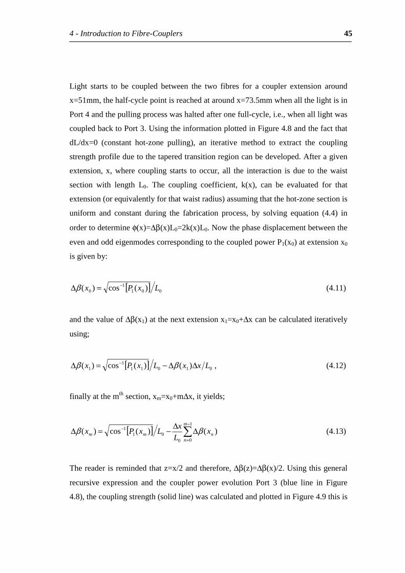
4-IntroductiontoFibre-Couplers 45
Light starts to be coupled between the two fibres for a coupler extension around
x=51mm,thehalf-cyclepointisreachedataroundx=73.5mmwhenallthelightisin
Port4andthepullingprocesswashaltedafteronefull-cycle,i.e.,whenalllightwas
coupledbacktoPort3.UsingtheinformationplottedinFigure4.8andthefactthat
dL/dx=0 (constant hot-zone pulling), an iterative method to extract the coupling
strengthprofileduetothetaperedtransitionregioncanbedeveloped.Afteragiven
extension,x,where coupling starts tooccur, all the interaction isdue to thewaist
section with length L0. The coupling coefficient, k(x), can be evaluated for that
extension(orequivalentlyforthatwaistradius)assumingthatthehot-zonesectionis
uniform and constant during the fabrication process, by solving equation (4.4) in
ordertodetermineφ(x)=∆β(x)L0=2k(x)L0.Nowthephasedisplacementbetweenthe
evenandoddeigenmodescorrespondingtothecoupledpowerP1(x0)atextensionx0
isgivenby:
[ ] 0011
0 )(cos)( LxPx −=∆β (4.11)
andthevalueof∆β(x1)atthenextextensionx1=x0+∆xcanbecalculatediteratively
using;
[ ] 010111
1 )()(cos)( LxxLxPx ∆∆−=∆ − ββ , (4.12)
finallyatthemthsection,xm=x0+m∆x,ityields;
[ ] −
=
− ∆∆−=∆1
0001
1 )()(cos)(m
nnmm x
Lx
LxPx ββ (4.13)
Thereaderisremindedthatz=x/2andtherefore,∆β(z)=∆β(x)/2.Usingthisgeneral
recursive expression and the coupler power evolution Port 3 (blue line in Figure
4.8),thecouplingstrength(solidline)wascalculatedandplottedinFigure4.9thisis
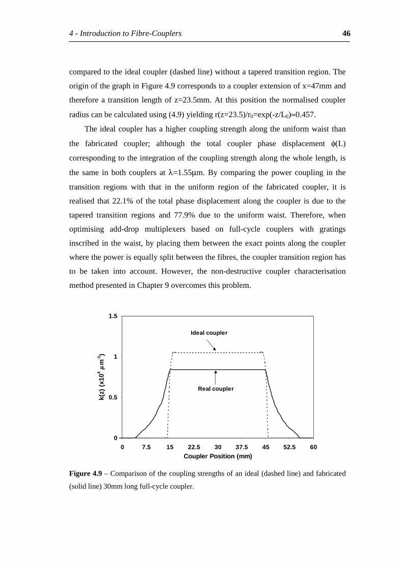
4-IntroductiontoFibre-Couplers 46
comparedtotheidealcoupler(dashedline)withoutataperedtransitionregion.The
originofthegraphinFigure4.9correspondstoacouplerextensionofx=47mmand
thereforea transition lengthofz=23.5mm.At thisposition thenormalisedcoupler
radiuscanbecalculatedusing(4.9)yieldingr(z=23.5)/r0=exp(-z/L0)≈0.457.
Theidealcouplerhasahighercouplingstrengthalongtheuniformwaist than
the fabricated coupler; although the total coupler phase displacement φ(L)
correspondingtotheintegrationofthecouplingstrengthalongthewholelength,is
the same in both couplers at λ=1.55µm. By comparing the power coupling in the
transition regions with that in the uniform region of the fabricated coupler, it is
realised that22.1%of the totalphasedisplacementalong thecoupler isdue to the
tapered transition regions and 77.9% due to the uniform waist. Therefore, when
optimising add-drop multiplexers based on full-cycle couplers with gratings
inscribed in thewaist,byplacing thembetween theexactpointsalong thecoupler
wherethepowerisequallysplitbetweenthefibres,thecouplertransitionregionhas
to be taken into account. However, the non-destructive coupler characterisation
methodpresentedinChapter9overcomesthisproblem.
0
0.5
1
1.5
0 7.5 15 22.5 30 37.5 45 52.5 60CouplerPosition(mm)
k(z)
(x1
04 m
-1)
Idealcoupler
Realcoupler
Figure4.9–Comparisonofthecouplingstrengthsofanideal(dashedline)andfabricated
(solidline)30mmlongfull-cyclecoupler.
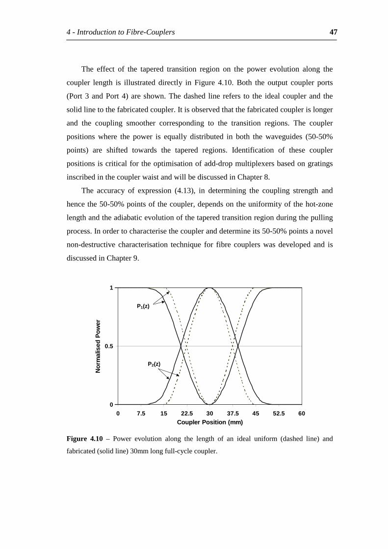
4-IntroductiontoFibre-Couplers 47
The effect of the tapered transition region on the power evolution along the
coupler length is illustrated directly in Figure 4.10. Both the output coupler ports
(Port3andPort4)are shown.Thedashed line refers to the idealcouplerand the
solidlinetothefabricatedcoupler.Itisobservedthatthefabricatedcouplerislonger
and the coupling smoother corresponding to the transition regions. The coupler
positions where the power is equally distributed in both the waveguides (50-50%
points) are shifted towards the tapered regions. Identification of these coupler
positionsiscriticalfortheoptimisationofadd-dropmultiplexersbasedongratings
inscribedinthecouplerwaistandwillbediscussedinChapter8.
The accuracy of expression (4.13), in determining the coupling strength and
hencethe50-50%pointsofthecoupler,dependsontheuniformityofthehot-zone
lengthandtheadiabaticevolutionofthetaperedtransitionregionduringthepulling
process.Inordertocharacterisethecoupleranddetermineits50-50%pointsanovel
non-destructive characterisation technique for fibre couplerswasdevelopedand is
discussedinChapter9.
0
0.5
1
0 7.5 15 22.5 30 37.5 45 52.5 60CouplerPosition(mm)
Nor
mal
ised
Pow
er
P1(z)
P2(z)
Figure 4.10 – Power evolution along the length of an ideal uniform (dashed line) and
fabricated(solidline)30mmlongfull-cyclecoupler.
4-IntroductiontoFibre-Couplers 48
4.3.6 Couplercrosssection
When fabricating couplers using the flame-brush technique, the degree of fusion
beforepullingthefibresdefinesthecrosssectionalshapeofthecoupler.Thehigher
the degree of fusion the closer the cross section of the fabricated coupler is to a
cylinder.Inthecaseofveryweakfusion,thecouplerhasacharacteristicdumbbell
shapeandforintermediatedegreesoffusion,thecross-sectionhasapproximatelyan
elliptical shape with varying eccentricity [67]. The theoretical description of the
couplerintermsofthecouplereigenmodes,alsoknownassupermodes,isrelatedto
thecouplercross-section,differentapproximationsforcalculatingthesemodeshave
beenaddressedintheliterature.InBureset.al.[68]thefibreswerenotfusedandthe
coreswereneglected;[69]approximatedthecouplercrosssectionusingdifferenta
rectangular cross section, and [70, 71] gives analytical expressions for the two
lowestordermodes,LP01andLP11,fordifferentcouplercross-sections(rectangular,
elliptical,circular)alsoneglectingthefibrecores.
Furtherwork, [67,72]usedaFieldCorrectionMethod toaccuratelycalculate
the coupler eigenmodes, while [73-75] use the rigorous surface integral equation
methoddeterminethecouplercharacteristics.
4.4 Summary
Fibrecouplersare importantcomponentsused inWDMsystems to routeandsplit
signals,monitorthenetwork,orcombinesignalandpumpwavelengthsforfeeding
optical amplifiers. Recently add-drop multiplexer configurations relying on the
inscriptionofBragggratingsinthecouplerwaisthavebeeninvestigated[41,42].In
order to optimise these devices accurate control of the fabrication and suitable
methods of characterisation for the couplers are required. In chapter 9 a non-
destructivemethodforcharacterisingfibre-couplersisdescribed.
In conclusion this chapter gave an introduction to coupler technologies and
described how light is transferred between the two waveguides along the coupler
length. A review of fibre-coupler fabrication technologies, their advantages and

4-IntroductiontoFibre-Couplers 49
drawbacksforeachwasdiscussed.Finallytheinfluenceofthefibrecouplerstapered
transitionregiononthepowerevolutionalongthecouplerlengthwasdescribed. It
willbeshown(inchapter8) that inorder tooptimiseanadd-dropmultiplexer; the
influenceofthetransitionregionhastobetakenintoaccount.
5
IntroductiontoFibre
BraggGratings
This chapter is a short introduction to fibre Bragg gratings aimed at providing a
fundamental understanding of the spectral properties of the filters designed using
thistechnology.Theconceptspresentedinthischapterareimportantfortheanalysis
andoptimisationofadd-dropmultiplexersbasedongratingsinscribedinthewaistof
fibre-couplers(chapter8).
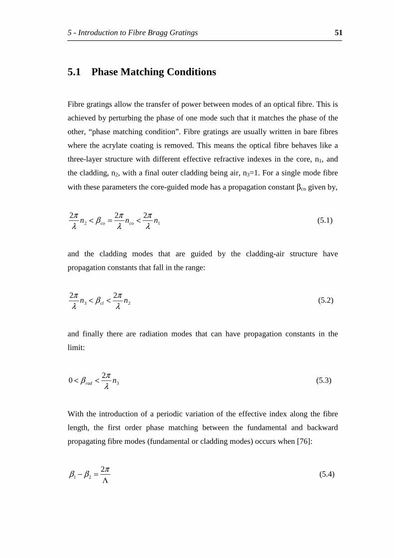
5-IntroductiontoFibreBraggGratings 51
5.1 PhaseMatchingConditions
Fibregratingsallowthetransferofpowerbetweenmodesofanopticalfibre.Thisis
achievedbyperturbingthephaseofonemodesuchthatitmatchesthephaseofthe
other,“phasematchingcondition”.Fibregratingsareusuallywritteninbarefibres
where theacrylatecoating is removed.Thismeans theoptical fibrebehaves likea
three-layer structurewithdifferent effective refractive indexes in the core, n1, and
thecladding,n2,withafinaloutercladdingbeingair,n3=1.Forasinglemodefibre
withtheseparametersthecore-guidedmodehasapropagationconstantβcogivenby,
12222
nnn coco λπ
λπβ
λπ <=< (5.1)
and the cladding modes that are guided by the cladding-air structure have
propagationconstantsthatfallintherange:
2322
nn cl λπβ
λπ << (5.2)
and finally there are radiation modes that can have propagation constants in the
limit:
32
0 nrad λπβ << (5.3)
With the introductionofaperiodicvariationof theeffective indexalong the fibre
length, the first order phase matching between the fundamental and backward
propagatingfibremodes(fundamentalorcladdingmodes)occurswhen[76]:
Λ=− πββ 2
21 (5.4)
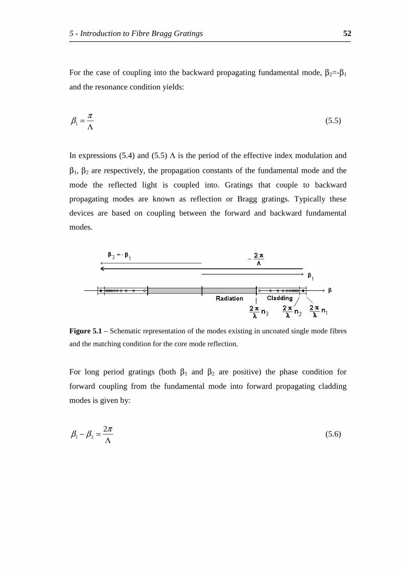
5-IntroductiontoFibreBraggGratings 52
For thecaseofcouplingintothebackwardpropagatingfundamentalmode,β2=-β1
andtheresonanceconditionyields:
Λ= πβ1 (5.5)
Inexpressions(5.4)and(5.5)Λistheperiodoftheeffectiveindexmodulationand
β1,β2arerespectively, thepropagationconstantsof thefundamentalmodeandthe
mode the reflected light is coupled into. Gratings that couple to backward
propagating modes are known as reflection or Bragg gratings. Typically these
devices are based on coupling between the forward and backward fundamental
modes.
Figure5.1–Schematicrepresentationofthemodesexistinginuncoatedsinglemodefibres
andthematchingconditionforthecoremodereflection.
For long period gratings (both β1 and β2 are positive) the phase condition for
forward coupling from the fundamental mode into forward propagating cladding
modesisgivenby:
Λ=− πββ 2
21 (5.6)
5-IntroductiontoFibreBraggGratings 53
5.2 MathematicalDescriptionofBraggGratings
This section describes a simple approach for obtaining the spectral properties of
fibreBragggratings.Foranextensivereviewof the theoryandpropertiesof fibre
Bragggratingsthereferences[77-79]aresuggested.
5.2.1 Coupledmodeequations
Coupledmodetheoryhasbeensuccessfullyusedtodescribethespectralproperties
ofBragggratings[78].RefractiveindexvariationswithaperiodΛalongthelength
ofafibrearegenerallyexpressedas:
( ))(2cos)()( 0 zznnzn θπ +Λ∆+= (5.7)
the functions∆n(z)andθ(z)are slowlyvarying functionscompared to thegrating
period Λ, n0 is the refractive index of the core, and ∆n(z) the envelope of the
refractive indexmodulation.Theparameter,θ(z), defines locally, thephaseof the
effectiveindexmodulation,whichisusedtodescribephaseshiftsorgratingchirp.
For simplicity this introduction will consider unchirped gratings only, therefore
θ(z)=0. Along the grating the forward propagating wave, v1, and backward
propagatingwave,v2,arerelatedbythecoupledmodeequations[80]:
1*
22
211
)(
)(
vziqvidzdv
vziqvidzdv
−+=
+−=
δ
δ (5.8)
where the amplitudes of the waves v1 and v2 are related to the amplitudes of the
forwardandbackwardpropagatingelectricfield,A(z)andB(z)respectively:
5-IntroductiontoFibreBraggGratings 54
zi
zi
evzB
evzAδ
δ
+
−
=
=
2
1
)(
)( , (5.9)
q(z)isthecouplingcoefficientgivenby:
)(2
)(0
znn
zq ∆Λ
= π (5.10)
and δ represents the detuning from the Bragg grating resonance wavelength,
λBragg=2n0Λ,definedas:
Λ−= π
λπδ 0
2n (5.11)
InthecaseofBragggratingswhere∆nvariesalongthegratinglengththespectral
characteristics canbeobtainedby solving thedifferential coupledmode equations
(5.8).Theparticularcaseofauniformgratinghasbeensolvedanalytically[81],the
reflectioncoefficientρ=v1(δ)/v2(δ)andreflectivityR=|ρ|2at thestartof thegrating
(z=0)are:
)cosh()sinh()sinh(
)(LiL
Lqγγγδ
γδρ+
−= (5.12)
222
2
)(cosh)(sinh
)(qL
LR
δγγδ−
= (5.13)
whereγ2=q2−δ2.
5-IntroductiontoFibreBraggGratings 55
Some important features can be inferred from these results. Firstly it can be
demonstrated that the maximum reflectivity Rmax occurs when the resonance
conditionisobserved,i.e.,δ=0andisgivenby
)(tanh2max qLR = (5.14)
and secondly the spectral bandwidth, ∆λzeros, defined as the two first zeros in
reflectivitycalculatedusing(5.13)yielding[78]:
2
0
1
∆+∆=∆
nLnn Braggzeros
λλ
λ (5.15)
For strong gratings where∆nL>>λBragg the normalised bandwidth is approximated
by:
0nnzeros ∆≈∆
λλ
(5.16)
andforweakgratingswhere∆nL<<λBraggthenormalisedbandwidthisapproximated
by:
LnBraggzeros
0
λλ
λ =∆ (5.17)
Whenwritinggratings in fibres, equation(5.15)providesuseful informationabout
the inducedeffective indexchangesimplybymeasuring thespectralbandwidthof
thegrating.Similarlyforuniformgratings,theinducedrefractiveindexchangecan
alsobecalculatedusing(5.14),bymeasuringthemaximumreflectivityattheBragg
wavelength.
5-IntroductiontoFibreBraggGratings 56
To fully understand the dispersive properties of fibre Bragg gratings the
conceptofgrouportimedelaymustbeintroduced.Forauniformgratingthetime
delay can be determined from the phase of the reflection coefficient ρ defined in
(5.12). Ifθρ=phase(ρ), thenthetimedelay,τρ, for lightreflectedfromagratingis
definedas[78]:
λθ
πλ
ωθ
τ ρρρ d
d
cd
d
2
2
−== (5.18)
andtheeffectivelength, leff, that lightataparticularwavelengthtravelswithinthe
gratingbeforeitreturnstotheorigincanbecalculatedfromleff=cτρ/n0. Inuniform
gratings,theminimumtimedelayoccursattheBraggwavelength.Forwavelengths
near the edges of the grating bandwidth and the sidelobes of the reflectivity, the
dispersion is greatest with the time delay varying rapidly with wavelength. Thus,
largetimedelaysarecharacteristicofthisregimeandareduetothesewavelengths
sufferingmultiplereflectionsbeforeexitingthegrating(asinaFabry-Perotcavity).
Figure5.2showsthereflectivityspectrumandthetimedelayforauniformgrating
withastrength,qL=4,andagratinglengthofL=20mm.Themaximumreflectivity,
whichcanbecalculated from(5.14), corresponds to theminimum timedelay.For
wavelengths near the first reflectivity zeros, the time delay is maximum
correspondingtoseveralround-tripsbeforethelightexiststhegrating.
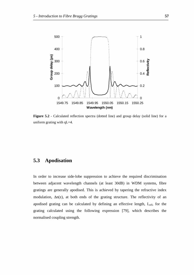
5-IntroductiontoFibreBraggGratings 57
0
100
200
300
400
500
1549.75 1549.85 1549.95 1550.05 1550.15 1550.25Wavelength(nm)
Gro
upd
elay
(ps
)
0
0.2
0.4
0.6
0.8
1
Ref
lect
ivity
Figure 5.2 - Calculated reflection spectra (dotted line) and group delay (solid line) for a
uniformgratingwithqL=4.
5.3 Apodisation
In order to increase side-lobe suppression to achieve the required discrimination
between adjacent wavelength channels (at least 30dB) in WDM systems, fibre
gratings are generally apodised. This is achieved by tapering the refractive index
modulation, ∆n(z), at both ends of the grating structure. The reflectivity of an
apodised grating can be calculated by defining an effective length, Leff, for the
grating calculated using the following expression [79], which describes the
normalisedcouplingstrength.
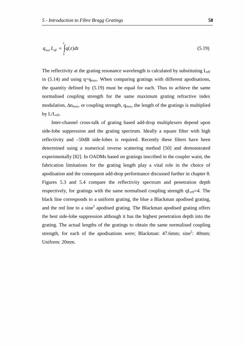
5-IntroductiontoFibreBraggGratings 58
=L
eff dzzqLq0
max )( (5.19)
ThereflectivityatthegratingresonancewavelengthiscalculatedbysubstitutingLeff
in (5.14) and using q=qmax. When comparing gratings with different apodisations,
the quantity defined by (5.19) must be equal for each. Thus to achieve the same
normalised coupling strength for the same maximum grating refractive index
modulation,∆nmax,orcouplingstrength,qmax,thelengthofthegratingsismultiplied
byL/Leff.
Inter-channel cross-talk of grating based add-drop multiplexers depend upon
side-lobe suppression and the grating spectrum. Ideally a square filter with high
reflectivity and –50dB side-lobes is required. Recently these filters have been
determined using a numerical inverse scattering method [50] and demonstrated
experimentally[82].InOADMsbasedongratingsinscribedinthecouplerwaist,the
fabrication limitations for the grating length play a vital role in the choice of
apodisationandtheconsequentadd-dropperformancediscussedfurtherinchapter8.
Figures 5.3 and 5.4 compare the reflectivity spectrum and penetration depth
respectively, forgratingswith the samenormalisedcouplingstrengthqLeff=4.The
blacklinecorrespondstoauniformgrating,theblueaBlackmanapodisedgrating,
andtheredlinetoasine2apodisedgrating.TheBlackmanapodisedgratingoffers
thebestside-lobesuppressionalthoughithasthehighestpenetrationdepthintothe
grating.Theactual lengthsof thegratings toobtain the samenormalisedcoupling
strength, for each of the apodisations were; Blackman: 47.6mm; sine2: 40mm;
Uniform:20mm.
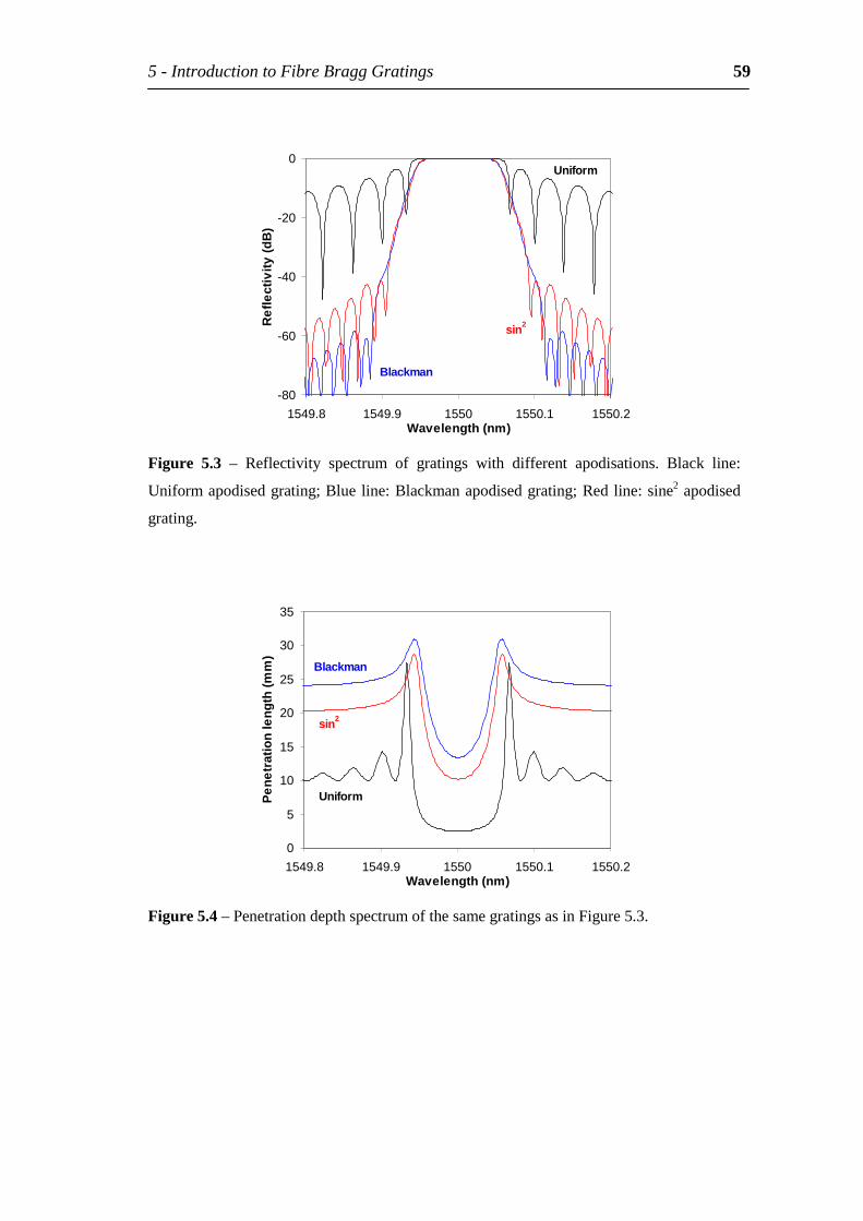
5-IntroductiontoFibreBraggGratings 59
-80
-60
-40
-20
0
1549.8 1549.9 1550 1550.1 1550.2Wavelength(nm)
Ref
lect
ivity
(dB
)
Blackman
sin2
Uniform
Figure 5.3 – Reflectivity spectrum of gratings with different apodisations. Black line:
Uniformapodisedgrating;Blueline:Blackmanapodisedgrating;Redline:sine2apodised
grating.
0
5
10
15
20
25
30
35
1549.8 1549.9 1550 1550.1 1550.2Wavelength(nm)
Pen
etra
tion
leng
th(m
m)
Blackman
sin2
Uniform
Figure5.4–PenetrationdepthspectrumofthesamegratingsasinFigure5.3.
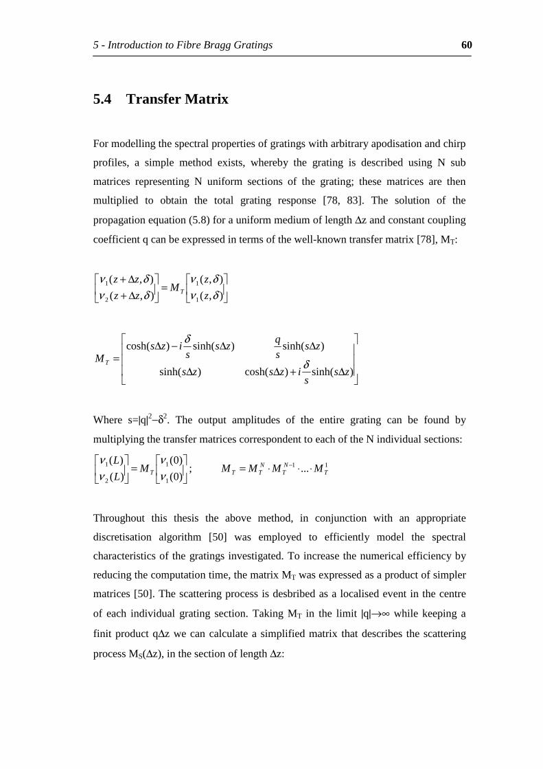
5-IntroductiontoFibreBraggGratings 60
5.4 TransferMatrix
Formodellingthespectralpropertiesofgratingswitharbitraryapodisationandchirp
profiles, a simple method exists, whereby the grating is described using N sub
matrices representing N uniform sections of the grating; these matrices are then
multiplied to obtain the total grating response [78, 83]. The solution of the
propagationequation(5.8)forauniformmediumoflength∆zandconstantcoupling
coefficientqcanbeexpressedintermsofthewell-knowntransfermatrix[78],MT:
=
∆+∆+
),(),(
),(),(
1
1
2
1
δνδν
δνδν
z
zM
zz
zzT
∆+∆∆
∆∆−∆=
)sinh()cosh()sinh(
)sinh()sinh()cosh(
zss
izszs
zssq
zss
izsMT δ
δ
Where s=|q|2−δ2. The output amplitudes of the entire grating can be found by
multiplyingthetransfermatricescorrespondenttoeachoftheNindividualsections:
=
)0()0(
)()(
1
1
2
1
νν
νν
TML
L; 11 ... T
NT
NTT MMMM ⋅⋅⋅= −
Throughout this thesis the above method, in conjunction with an appropriate
discretisation algorithm [50] was employed to efficiently model the spectral
characteristicsofthegratingsinvestigated.Toincreasethenumericalefficiencyby
reducingthecomputationtime,thematrixMTwasexpressedasaproductofsimpler
matrices[50].Thescatteringprocessisdesbribedasalocalisedeventinthecentre
of each individual grating section. Taking MT in the limit |q|→∞ whilekeeping a
finitproductq∆zwecancalculateasimplifiedmatrix thatdescribes thescattering
processMS(∆z),inthesectionoflength∆z:
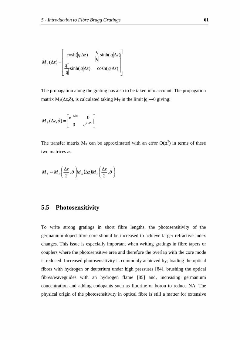
5-IntroductiontoFibreBraggGratings 61
∆∆
∆∆=∆
)cosh()sinh(
)sinh()cosh(
)( *
zqzqqq
zqqq
zq
zM S
Thepropagationalongthegratinghasalsotobetakenintoaccount.Thepropagation
matrixMP(∆z,δ),iscalculatedtakingMTinthelimit|q|→0giving:
=∆ ∆+
∆−
zi
zi
P e
ezM δ
δ
δ0
0),(
ThetransfermatrixMTcanbeapproximatedwithanerrorO(∆3) in termsof these
twomatricesas:
( ) .,2
,2
∆∆
∆≈ δδ zMzM
zMM PSPT
5.5 Photosensitivity
To write strong gratings in short fibre lengths, the photosensitivity of the
germanium-dopedfibrecoreshouldbe increased toachieve larger refractive index
changes.This issueisespeciallyimportantwhenwritinggratingsinfibre tapersor
couplerswherethephotosensitiveareaandthereforetheoverlapwiththecoremode
isreduced.Increasedphotosensitivityiscommonlyachievedby;loadingtheoptical
fibres with hydrogen or deuterium under high pressures [84], brushing the optical
fibres/waveguides with an hydrogen flame [85] and, increasing germanium
concentration and adding codopants such as fluorine or boron to reduce NA. The
physicaloriginof thephotosensitivityinopticalfibreisstillamatterforextensive
5-IntroductiontoFibreBraggGratings 62
discussionsandisoutofthecontextofthisthesis.Forgoodreviewsconcerningthe
photosensitizationprocess,readersarereferredto[86-88].
5.6 Summary
AbriefintroductiontofibreBragggratingswaspresentedinthissection.Thephase
matchingbetweenforwardandbackwardpropagatingfundamentalfibremodescan
be achieved with a periodic variation of the effective index. The interaction is
quantifiedusing thewell knowncoupledmode equations.Analytical solutions for
theseequationsexistfor thesimplestcaseofauniformgrating.Forusefuldevices
withlowsidelobes,inordertoaccuratelydiscriminatebetweenadjacentchannels,
differentfibreapodisationsareused.Thespectralresponseofgratingswitharbitrary
apodisations is obtainedby solving the coupled modeequationsusing an efficient
scatteringmatrixmodel.Theconceptoftimedelayandpenetrationdepthoflightin
thegratingwereintroducedaswellinordertooptimisetheperformanceofadd-drop
multiplexersbasedongratingsinscribedinthewaistoffibrecouplers,discussedin
chapter8.
6
Acousto-OpticTunable
FilterDesign
InthischapteramethodfortailoringtheshapeoflossfiltersbasedontheAcousto-
optic(AO)interactionintaperedopticalfibresispresented.Themethodisbasedon
the coupling of light from the fundamental core mode to the fibre taper cladding
modes. The conditions for resonant coupling between the modes in tapered fibres
arecharacterisedandasanapplicationa filter isdesigned todynamicallyequalise
theEDFAgainspectrumwithreducedtuningparameters.

6-Acousto-OpticTunableFilterDesign 64
6.1 Acousto-opticTechnology
Acousto-optic (AO) interaction in optical fibres results from the coupling of light
between the propagation modes of an optical fibre, induced by an acoustic wave.
Frequency shifters, switches, filters, amplitude modulators [16, 17, 26, 89-93, 94,
95-98]areexamplesofpracticaldevicesusingthistechnology.Earlyacousto-optic
devicesreliedonthecouplinginatwo-modefibre[26,99].Inthiscase,aflexural
acoustic wave couples light from the fundamental mode (LP01) to a low-order
claddingmode(LP11).Thesedeviceswereusedasfrequencyshiftersandlossfilters.
Other AO devices were based on the coupling between the modes of a dual-core
opticalfibre[90],orsimilarly,thepolarisationmodesofahighbirefringentoptical
fibre[89].AnewrangeofAOdevicesmakeuseoftaperedfibrestructures[91-93,
100]. Null couplers were used in different configurations giving rise to frequency
shifters, acousticmodulators and switches. In this case, theAO interactionoccurs
betweentheopticalmodessupportedbythethinsilicawaist(witharadiusofafew
microns).Theresidualcoredoesnotconfinethesemodes.Theycanbeconsidered
cladding modes, propagated by the whole silica-air structure. One of the main
advantages of the tapered AO devices is their low power consumption due to the
amplificationoftheacousticwaveinthetaperedregion[64].
Recently,wide interest hasbeendevoted tonovelAO tunable filters [16,17,
26]. Inthesefilters, light iscoupledfromthefundamentalmode(LP01)ofasingle
modeoptical fibretoseveral lowordercladdingmodes(LP11,LP12,LP13) through
anacousticflexuralwave.ThemainfeatureofAOfilterswithrespecttostaticfilters
such as long period gratings [97], is the ability to control dynamically the loss
spectrum in order to compensate for gain saturation effects of optical amplifiers
caused by power fluctuations of the input signal. By changing the acoustic wave
frequencyandamplitudeonecanchangetheresonancewavelengthandstrengthof
the AO interaction, this is to reconfigure the filter loss spectrum to the desired
response.
6-Acousto-OpticTunableFilterDesign 65
ThedevicepresentedbyKimetal.[16,17,98]isveryflexibleinreconfiguring
thespectralresponseoftheAOfilter.However,thatflexibilityrelieson6acoustic
wave frequencies with different powers. This means that for tuning the spectral
response of the filter 12 parameters need to be adjusted, which represents a very
complexsystem.
In this chapter an alternativedesign thatusesonly2parameters for adjusting
dynamically the filter response is presented. To demonstrate the operation of the
device,thedesignedfilterwasusedtoflattentheASEspectrumofanerbiumdoped
fibre amplifier (EDFA) for different saturation levels. The effect of a controlled
tapering of a single mode optical fibre on the coupling between the fundamental
modeandlowordercladdingmodesisinvestigated.Thecontroloftheradiusprofile
alonganon-uniformtaperedregionofthefibrecanberegardedasanotherdegreeof
freedomfor tailoringthespectralresponseof theAOfilter.Usingthisapproach,a
singleacousticfrequencycanbeusedwiththespectralcharacteristicsrelyingonthe
complexmulti-taper structure.Consequently there is a reductionof thenumberof
parametersneededtotunethefilterdynamicallybutasacompromise,areductionof
itsflexibility.
The acoustic interaction in tapered fibres has been studied in this work. This
interaction results from the exchange of power between two light modes of the
opticalfibre,duetoaperiodicperturbationintherefractiveindex.Theperturbation
is induced by an acoustic wave that acts like a periodic grating. The resonance
condition for this power exchange requires that the beatlength, LB, of the modes
matchtheacousticwavelength,Λ,intheinteractionregion.Coupledmodeequations
areusedtoquantifytheamountoflightcoupledfromonemodetotheotherdueto
theperturbation.Theamountofopticalpowercoupleddependsontheamplitudeof
theacousticwave,theoverlapbetweentheopticalmodesandtheelasticproperties
ofthefibre.Inthiswork,thecouplingbetweenthefundamentalmodeLP01andthe
lowerordercladdingmodesLP11,LP12andLP13intaperedfibresisstudied.
The effect of tapering a fibre is to change the dispersion relations of the
different optical modes, inducing differences in the beatlength between the
fundamental mode and the cladding modes. These dispersion relations were fully
6-Acousto-OpticTunableFilterDesign 66
characterisedboththeoreticallyandexperimentally.Theyarethebasisfordesigning
structures of different tapers and interaction lengths with different spectral
responses.
6.2 Theory
ThissectiongivesthetheoreticalbackgroundforcharacterisingtheAOinteraction
intaperedopticalfibres.Firstthepropagationofacousticwavesinopticalfibresis
analysed.Then,thepropagationoftheopticalmodesintaperedfibresisdescribed.
Finally, the interactionbetween the acousticwaveand theoptical fibremodes are
quantifiedusingcoupledmodetheory.
6.2.1 Propagationoftheacousticwave
Thepropagationofacousticwavesinrodsandcladrodsmadefromisotropiclinear
materials has been extensively studied [101]. Torsional, longitudinal and flexural
wavemotionsarepermittedinthesestructures.Atlowfrequencies,aflexuralwave
propagating along a fibre can be described approximately by the Euler-Bernoulli
theoryofbeams[101].Ifu(z,t)isthetransversedisplacementfromtheequilibrium
axis then the equation describing the propagation of the flexural acoustic wave is
[59]:
0),(1 2
224 =
+− tzuppYIT
p tzz α (6.1)
n
n
xAYI
∂∂== n
x2 pandwith
ρα
WhereTistheaxialtensionappliedtothefibre,YistheYoungModulus,ρisthe
densityofthematerial,Aistheareaofthecrosssection(A=πr2)andIthemoment
6-Acousto-OpticTunableFilterDesign 67
ofinertia(I=πr4/4foracylinder).Inthecasewherenotensionisappliedtothesilica
fibre (T=0) then equation (6.1) simplifies and considering solutions of the form
u(z,t)=U(0)e-iKzeiΩtthedispersionrelationscanbefoundtobe:
RVK
ext
Ω=Λ
= 22π (6.2)
WhereKisthepropagationconstantoftheacousticflexuralwave,Ωistheangular
frequency,R is thefibre radiusandVext is thevelocityof theextensionalwave in
silica(Vext=(Y/ρ)1/2=5760ms-1).Atlowfrequencies,thepowerflowoftheflexural
acousticwaveisgivenby[102]:
( ) 20
21
55720
23 2)(2 ufRVufRvP extg πρρπ == (6.3)
Wherevg is thegroupvelocityof thewave(vg=∂Ω/∂K),u0 is theamplitudeof the
acousticwaveandfistheacousticfrequency.
6.2.1.1 Effect of tension applied to the fibre
Iftensionisappliedtothefibrethenthesecondterminequation(6.1)accountsfor
its effect on the propagation of the acoustic wave (T≠0). The roots of the
characteristicequationobtainedbysubstitutingu(z,t)=U(0)e-iKzeiΩtin(6.1)are:
21
21
2
22
Ω+±±=α
γγK (6.4)
Whereγ=T/(2YI).Consideringanappliedtension,theacousticpropagationconstant
willbeperturbedaccordingto,
6-Acousto-OpticTunableFilterDesign 68
AIYVT
KdK ext 1
4Ω= (6.5)
AccordingtoHooke’ slawthestrainandtensionappliedtothefibrecanberelated,
forsmallstrains,by:
YAT
S z = (6.6)
6.2.2 Opticalmodesintaperedfibres
A single mode optical fibre is a three-layer structure (core/cladding/air), which
supportsseveralcladdingmodesbesidesthefundamentalmode,guidedbythecore.
Thecladdingmodesareprimarilyguidedbythecladding/airstructure.Bytapering
the fibre, the modes will change their optical properties. If the taper is smooth
enough, the modes will evolve adiabatically, maintaining their identity with
insignificant lossesduring their propagation.The electric fieldof anopticalmode
propagatingalongthetapercanbewrittenas:
( ) ( ) tjdj
mnmnmn
z
mn
eezbrEzAtzrE ωξξβ
φφ
=−
0
)(
)(,,)(,,,
(6.7)
Where βmn(z) is the propagation constant of the mode LPmn, ωmn is its angular
frequency,b(z) the taper radiusatpointz,Emn is thenormalisedfieldpattern,and
Amn(z) is a slowlyvaryingamplitude.βmn(z) andEmn dependon the radiusof the
taper. βmn(z) is considered as a local propagation constant and Emn the local
normalised field pattern. If the taper is smooth enough to allow adiabatic
propagationwithoutlossesandtransferofpowerbetweenthemodes,thenAmn(z)is
constant,independentoftheposition.
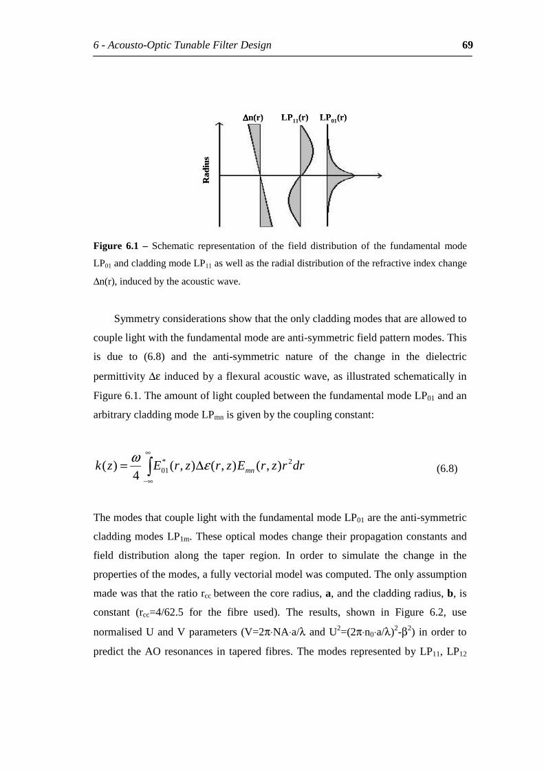
6-Acousto-OpticTunableFilterDesign 69
LP01(r)LP11(r)∆∆∆∆n(r)
Rad
ius
LP01(r)LP11(r)∆∆∆∆n(r)
Rad
ius
Figure 6.1 – Schematic representation of the field distribution of the fundamental mode
LP01andcladdingmodeLP11aswellastheradialdistributionoftherefractiveindexchange
∆n(r),inducedbytheacousticwave.
Symmetryconsiderationsshowthattheonlycladdingmodesthatareallowedto
couplelightwiththefundamentalmodeareanti-symmetricfieldpatternmodes.This
is due to (6.8) and the anti-symmetric nature of the change in the dielectric
permittivity∆ε inducedbyaflexuralacousticwave,as illustratedschematicallyin
Figure6.1.TheamountoflightcoupledbetweenthefundamentalmodeLP01andan
arbitrarycladdingmodeLPmnisgivenbythecouplingconstant:
∞
∞−
∆= drrzrEzrzrEzk mn2*
01 ),(),(),(4
)( εω (6.8)
ThemodesthatcouplelightwiththefundamentalmodeLP01aretheanti-symmetric
claddingmodesLP1m.Theseopticalmodeschangetheirpropagationconstantsand
field distribution along the taper region. In order to simulate the change in the
propertiesofthemodes,afullyvectorialmodelwascomputed.Theonlyassumption
madewasthattheratiorccbetweenthecoreradius,a,andthecladdingradius,b,is
constant (rcc=4/62.5 for the fibre used). The results, shown in Figure 6.2, use
normalisedUandVparameters (V=2π⋅NA⋅a/λandU2=(2π⋅n0⋅a/λ)2-β2) inorder to
predict theAOresonances in taperedfibres.ThemodesrepresentedbyLP11,LP12
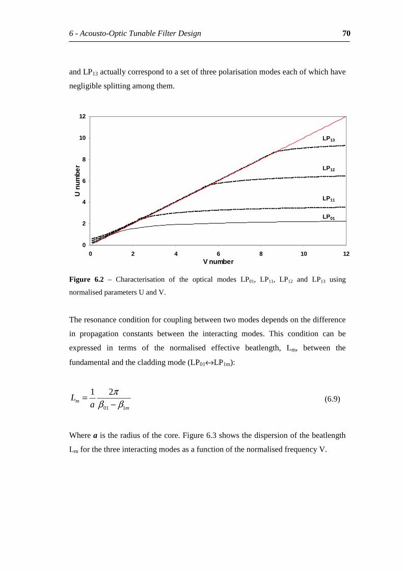
6-Acousto-OpticTunableFilterDesign 70
andLP13actuallycorrespondtoasetofthreepolarisationmodeseachofwhichhave
negligiblesplittingamongthem.
0
2
4
6
8
10
12
0 2 4 6 8 10 12Vnumber
Un
umbe
r
LP13
LP12
LP11
LP01
Figure 6.2 – Characterisation of the optical modes LP01, LP11, LP12 and LP13 using
normalisedparametersUandV.
Theresonanceconditionforcouplingbetweentwomodesdependsonthedifference
in propagation constants between the interacting modes. This condition can be
expressed in terms of the normalised effective beatlength, Lm, between the
fundamentalandthecladdingmode(LP01↔LP1m):
mm a
L101
21ββ
π−
= (6.9)
Whereaistheradiusofthecore.Figure6.3showsthedispersionofthebeatlength
LmforthethreeinteractingmodesasafunctionofthenormalisedfrequencyV.
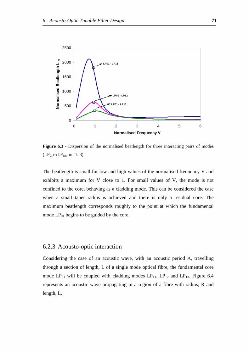
6-Acousto-OpticTunableFilterDesign 71
0
500
1000
1500
2000
2500
0 1 2 3 4 5 6
NormalisedFrequencyV
Nor
mal
ised
Bea
tleng
thL
mLP01-LP11
LP01-LP12
LP01-LP13
Figure6.3 -Dispersionof thenormalisedbeatlength for three interactingpairsofmodes
(LP01↔LP1m,m=1..3).
ThebeatlengthissmallforlowandhighvaluesofthenormalisedfrequencyVand
exhibits a maximum for V close to 1. For small values of V, the mode is not
confinedtothecore,behavingasacladdingmode.Thiscanbeconsideredthecase
when a small taper radius is achieved and there is only a residual core. The
maximum beatlength corresponds roughly to the point at which the fundamental
modeLP01beginstobeguidedbythecore.
6.2.3 Acousto-opticinteraction
Considering the case of an acoustic wave, with an acoustic period Λ, travelling
throughasectionof length,Lofasinglemodeopticalfibre, thefundamentalcore
mode LP01 will be coupled with cladding modes LP11, LP12 and LP13. Figure 6.4
represents an acoustic wave propagating in a region of a fibre with radius, R and
length,L.
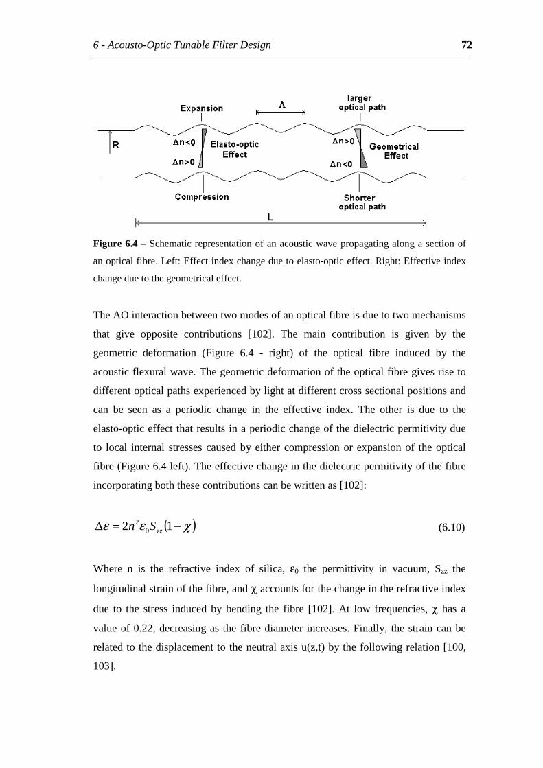
6-Acousto-OpticTunableFilterDesign 72
Figure6.4–Schematicrepresentationofanacousticwavepropagatingalongasectionof
anopticalfibre.Left:Effectindexchangeduetoelasto-opticeffect.Right:Effectiveindex
changeduetothegeometricaleffect.
TheAOinteractionbetweentwomodesofanopticalfibreisduetotwomechanisms
that give opposite contributions [102]. The main contribution is given by the
geometric deformation (Figure 6.4 - right) of the optical fibre induced by the
acousticflexuralwave.Thegeometricdeformationoftheopticalfibregivesriseto
differentopticalpathsexperiencedbylightatdifferentcrosssectionalpositionsand
can be seen as a periodic change in the effective index. The other is due to the
elasto-opticeffectthatresultsinaperiodicchangeofthedielectricpermitivitydue
to local internal stresses causedbyeither compressionor expansionof theoptical
fibre(Figure6.4left).Theeffectivechangeinthedielectricpermitivityofthefibre
incorporatingboththesecontributionscanbewrittenas[102]:
( )χεε −=∆ 12 02
zzSn (6.10)
Where n is the refractive index of silica, ε0 the permittivity in vacuum, Szz the
longitudinalstrainofthefibre,andχaccountsforthechangeintherefractiveindex
due to the stress induced by bending the fibre [102]. At low frequencies, χ has a
valueof0.22,decreasingas thefibrediameter increases.Finally, thestraincanbe
relatedtothedisplacementtotheneutralaxisu(z,t)bythefollowingrelation[100,
103].
6-Acousto-OpticTunableFilterDesign 73
2
2
2
2 ),(4Λ
−== ytzuy
dzud
S zzπ
(6.11)
whereyistheradialpositioninthedirectionofthefibredisplacement.
Theresonanceconditionforthecouplingbetweentwoopticalmodesdependsonthe
dispersion relations of the modes as well as the period of the acoustic wave.
Momentum conservation requirements establish the following condition for
resonancecoupling:
Lm(λr,b)=Λ(b,Ω) (6.12)
From equation (6.12) we observe that the beatlength, Lm, between the interacting
modesisequaltotheacousticwavelength,Λ,forresonancecoupling.Theresonance
wavelength,λr,oftheinteractingmodescanbecalculatedasafunctionofthetaper
radius, a, by intersecting the normalised beatlength with the acoustic wavelength.
TheseresultsareshowninFigure6.5.Theyrepresenttheresonancewavelengthof
thethreeAOinteractionsobservedexperimentally,asafunctionofthetaperradius
andforthreeacousticfrequencies1.15MHz,1.25MHzand1.35MHz.
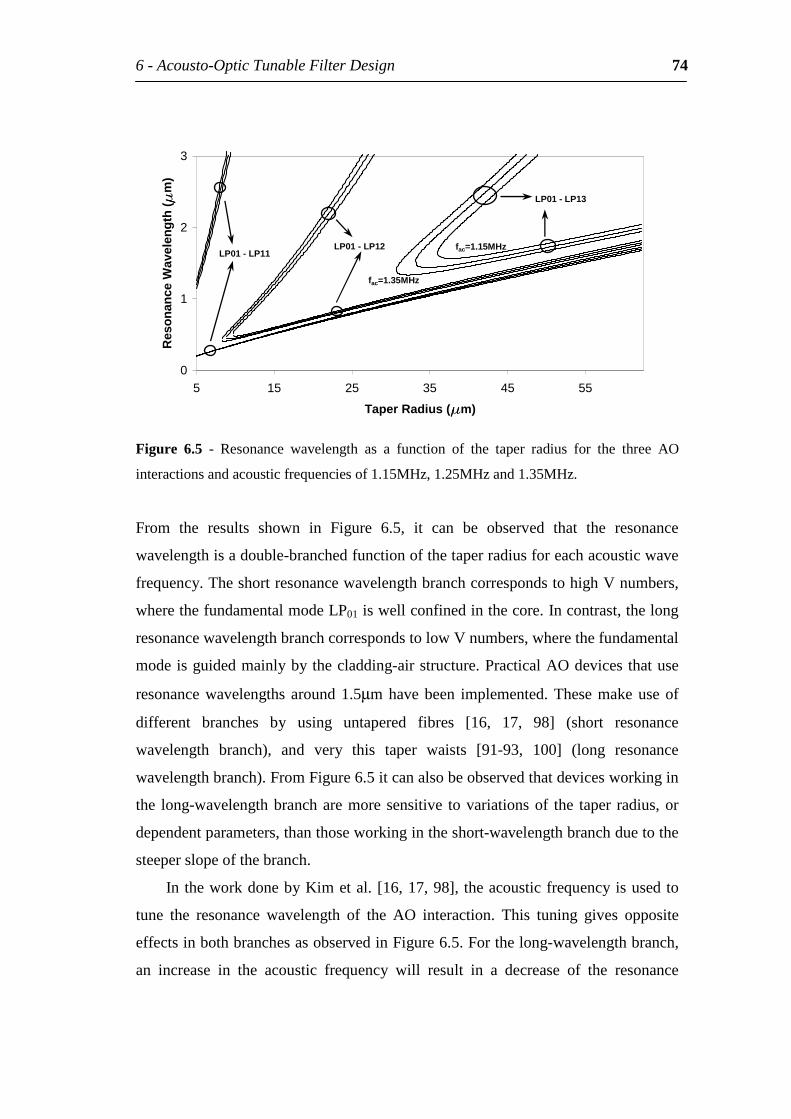
6-Acousto-OpticTunableFilterDesign 74
0
1
2
3
5 15 25 35 45 55
TaperRadius(m)
Res
onan
ceW
avel
engt
h(
m)
LP01-LP12LP01-LP11
LP01-LP13
fac=1.35MHz
fac=1.15MHz
Figure 6.5 - Resonance wavelength as a function of the taper radius for the three AO
interactionsandacousticfrequenciesof1.15MHz,1.25MHzand1.35MHz.
From the results shown in Figure 6.5, it can be observed that the resonance
wavelengthisadouble-branchedfunctionofthetaperradiusforeachacousticwave
frequency.TheshortresonancewavelengthbranchcorrespondstohighVnumbers,
wherethefundamentalmodeLP01iswellconfinedinthecore.Incontrast,thelong
resonancewavelengthbranchcorrespondstolowVnumbers,wherethefundamental
modeisguidedmainlybythecladding-airstructure.PracticalAOdevicesthatuse
resonancewavelengths around1.5µmhavebeen implemented.Thesemakeuseof
different branches by using untapered fibres [16, 17, 98] (short resonance
wavelength branch), and very this taper waists [91-93, 100] (long resonance
wavelengthbranch).FromFigure6.5itcanalsobeobservedthatdevicesworkingin
the long-wavelengthbrancharemore sensitive tovariationsof the taper radius,or
dependentparameters,thanthoseworkingintheshort-wavelengthbranchduetothe
steeperslopeofthebranch.
IntheworkdonebyKimetal.[16,17,98],theacousticfrequencyisusedto
tune the resonance wavelength of the AO interaction. This tuning gives opposite
effectsinbothbranchesasobservedinFigure6.5.Forthelong-wavelengthbranch,
an increase in the acoustic frequency will result in a decrease of the resonance
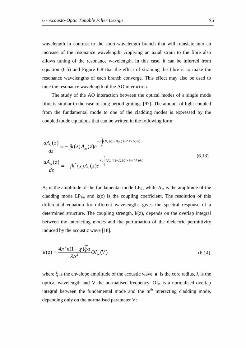
6-Acousto-OpticTunableFilterDesign 75
wavelength in contrast to the short-wavelength branch that will translate into an
increase of the resonance wavelength. Applying an axial strain to the fibre also
allows tuning of the resonance wavelength. In this case, it can be inferred from
equation (6.5) and Figure 6.8 that the effect of straining the fibre is to make the
resonance wavelengths of each branch converge. This effect may also be used to
tunetheresonancewavelengthoftheAOinteraction.
The studyof theAO interactionbetween theopticalmodesof a single mode
fibreissimilartothecaseoflongperiodgratings[97].Theamountoflightcoupled
from the fundamental mode to one of the cladding modes is expressed by the
coupledmodeequationsthatcanbewritteninthefollowingform:
−=
−=
Λ⋅+−+
Λ⋅+−−
z
m
z
m
djm
dj
m
ezAzjkdz
zdA
ezAzjkdz
zdA
0
0
00
)/2)()((
0*
)/2)()((0
)()()(
)()()(
ξπξβξβ
ξπξβξβ
(6.13)
A0istheamplitudeofthefundamentalmodeLP01whileAmistheamplitudeofthe
cladding mode LP1m and k(z) is the coupling coefficient. The resolution of this
differential equation for different wavelengths gives the spectral response of a
determined structure. The coupling strength, k(z), depends on the overlap integral
between the interacting modes and the perturbation of the dielectric permittivity
inducedbytheacousticwave[18].
)(~
)1(4)( 2
4
VOIan
zk mΛ−=
λξχπ
(6.14)
whereξistheenvelopeamplitudeoftheacousticwave,a,isthecoreradius,λisthe
optical wavelength and V the normalised frequency. OIm is a normalised overlap
integral between the fundamental mode and the mth interacting cladding mode,
dependingonlyonthenormalisedparameterV:
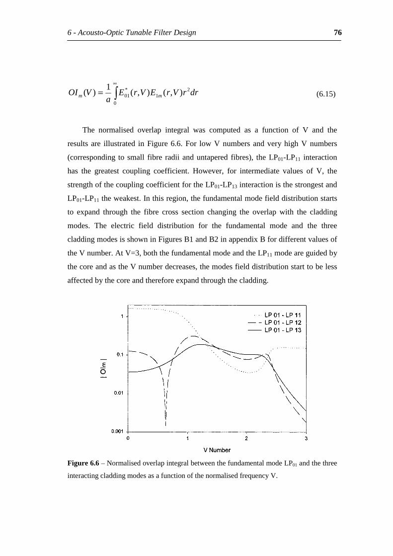
6-Acousto-OpticTunableFilterDesign 76
∞
=0
21
*01 ),(),(
1)( drrVrEVrE
aVOI mm (6.15)
The normalised overlap integral was computed as a function of V and the
resultsare illustrated inFigure6.6.For lowVnumbersandveryhighVnumbers
(corresponding to small fibre radii anduntapered fibres), theLP01-LP11 interaction
has the greatest coupling coefficient. However, for intermediate values of V, the
strengthofthecouplingcoefficientfortheLP01-LP13interactionisthestrongestand
LP01-LP11theweakest.Inthisregion,thefundamentalmodefielddistributionstarts
to expand through the fibre cross section changing the overlap with the cladding
modes. The electric field distribution for the fundamental mode and the three
claddingmodesisshowninFiguresB1andB2inappendixBfordifferentvaluesof
theVnumber.AtV=3,boththefundamentalmodeandtheLP11modeareguidedby
thecoreandastheVnumberdecreases,themodesfielddistributionstarttobeless
affectedbythecoreandthereforeexpandthroughthecladding.
Figure6.6–NormalisedoverlapintegralbetweenthefundamentalmodeLP01andthethree
interactingcladdingmodesasafunctionofthenormalisedfrequencyV.
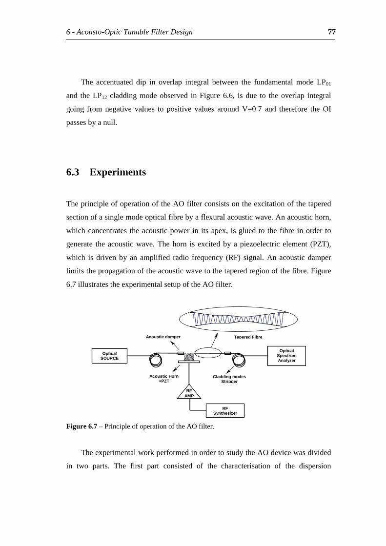
6-Acousto-OpticTunableFilterDesign 77
The accentuated dip in overlap integral between the fundamental mode LP01
and the LP12 claddingmodeobserved inFigure 6.6, is due to theoverlap integral
going from negative values to positive values around V=0.7 and therefore the OI
passesbyanull.
6.3 Experiments
TheprincipleofoperationoftheAOfilterconsistsontheexcitationofthetapered
sectionofasinglemodeopticalfibrebyaflexuralacousticwave.Anacoustichorn,
whichconcentrates theacousticpower in itsapex, isglued to thefibre inorder to
generate the acousticwave.Thehorn is excitedby apiezoelectric element (PZT),
which isdrivenby an amplified radio frequency (RF) signal. Anacousticdamper
limitsthepropagationoftheacousticwavetothetaperedregionofthefibre.Figure
6.7illustratestheexperimentalsetupoftheAOfilter.
RFAMP
RFSynthesizer
CladdingmodesStripper
AcousticHorn+PZT
OpticalSOURCE
OpticalSpectrumAnalyzer
TaperedFibreAcousticdamper
Figure6.7–PrincipleofoperationoftheAOfilter.
TheexperimentalworkperformedinordertostudytheAOdevicewasdivided
in two parts. The first part consisted of the characterisation of the dispersion
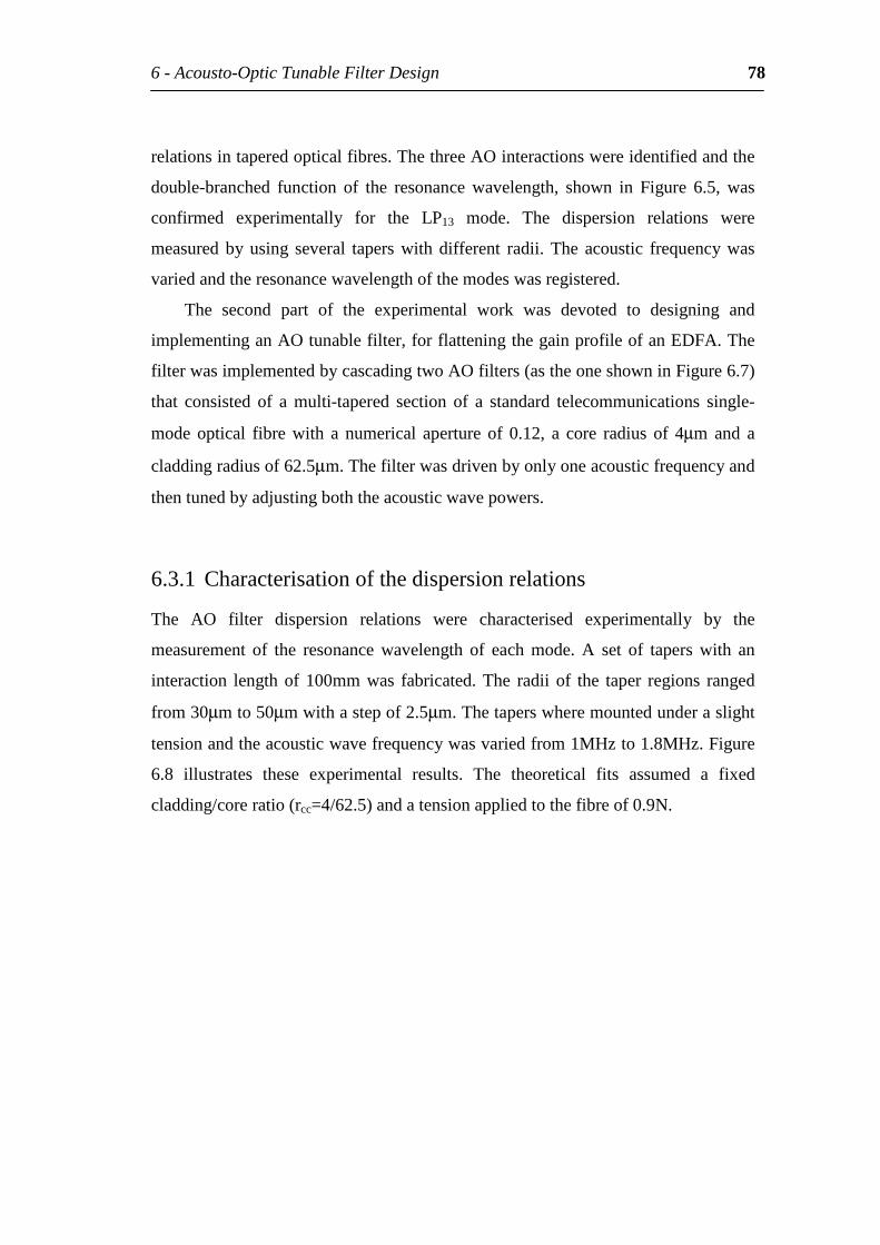
6-Acousto-OpticTunableFilterDesign 78
relationsintaperedopticalfibres.ThethreeAOinteractionswereidentifiedandthe
double-branched function of the resonance wavelength, shown in Figure 6.5, was
confirmed experimentally for the LP13 mode. The dispersion relations were
measuredbyusing several taperswithdifferent radii.The acoustic frequencywas
variedandtheresonancewavelengthofthemodeswasregistered.
The second part of the experimental work was devoted to designing and
implementinganAOtunablefilter,forflatteningthegainprofileofanEDFA.The
filterwasimplementedbycascadingtwoAOfilters(astheoneshowninFigure6.7)
that consisted of a multi-tapered section of a standard telecommunications single-
mode optical fibre with a numerical aperture of 0.12, a core radius of 4µm and a
claddingradiusof62.5µm.Thefilterwasdrivenbyonlyoneacousticfrequencyand
thentunedbyadjustingboththeacousticwavepowers.
6.3.1 Characterisationofthedispersionrelations
The AO filter dispersion relations were characterised experimentally by the
measurement of the resonance wavelength of each mode. A set of tapers with an
interaction lengthof100mmwas fabricated.The radii of the taper regions ranged
from30µmto50µmwithastepof2.5µm.Thetaperswheremountedunderaslight
tensionandtheacousticwavefrequencywasvariedfrom1MHzto1.8MHz.Figure
6.8 illustrates these experimental results. The theoretical fits assumed a fixed
cladding/coreratio(rcc=4/62.5)andatensionappliedtothefibreof0.9N.
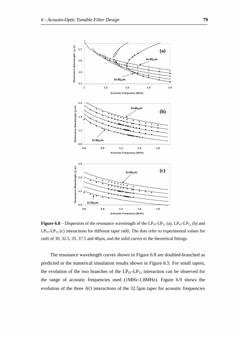
6-Acousto-OpticTunableFilterDesign 79
1.1
1.3
1.5
1.7
1 1.2 1.4 1.6 1.8
AcousticFrequency(M Hz)
Res
on
ance
Wav
elen
gth
m
(a)
0.9
1.1
1.3
1.5
0.6 0.9 1.2 1.5 1.8
AcousticFrequency(M Hz)
Res
on
ance
Wav
elen
gth
(
m)
(b)
0.9
1.1
1.3
1.5
0.6 0.9 1.2 1.5 1.8
AcousticFrequency(M Hz)
Res
on
ance
Wav
elen
gth
(
m)
(c)
b=40m
b=30m
b=30m
b=40m
b=30m
b=40m
Figure6.8–DispersionoftheresonancewavelengthoftheLP01-LP11(a),LP01-LP12(b)and
LP01-LP13(c)interactionsfordifferenttaperradii.Thedotsrefertoexperimentalvaluesfor
radiiof30,32.5,35,37.5and40m,andthesolidcurvestothetheoreticalfittings.
TheresonancewavelengthcurvesshowninFigure6.8aredoubled-branchedas
predictedinthenumericalsimulationresultsshowninFigure6.5.Forsmalltapers,
theevolutionof thetwobranchesof theLP01-LP13 interactioncanbeobservedfor
the range of acoustic frequencies used (1MHz-1.8MHz). Figure 6.9 shows the
evolutionofthethreeAOinteractionsofthe32.5µmtaperforacousticfrequencies
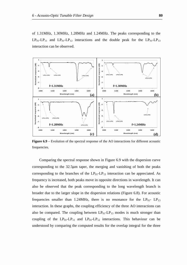
6-Acousto-OpticTunableFilterDesign 80
of 1.31MHz, 1.30MHz, 1.28MHz and 1.24MHz. The peaks corresponding to the
LP01-LP11 and LP01-LP12 interactions and the double peak for the LP01-LP13
interactioncanbeobserved.
-9
-7
-5
-3
-1
1
1000 1150 1300 1450 1600
W avelength(nm)
No
rmal
ised
res
po
nse
(d
B)
LP11-LP01 LP12-LP01
LP13-LP01
-9
-7
-5
-3
-1
1
1000 1150 1300 1450 1600
Wavelength(nm)
No
rmal
ised
res
po
nse
(d
B)
LP11-LP01 LP12-LP01
LP13-LP01
-9
-7
-5
-3
-1
1
1000 1150 1300 1450 1600
Wavelength(nm)
No
rmal
ised
res
po
nse
(d
B)
LP11-LP01 LP12-LP01 LP13-LP01
-9
-7
-5
-3
-1
1
1000 1150 1300 1450 1600
Wavelength(nm)
No
rmal
ised
res
po
nse
(d
B)
LP11-LP01 LP12-LP01
LP13-LP01
(a)
(c) (d)
(b)
f=1.31MHz f=1.30MHz
f=1.28MHz f=1.24MHz
Figure6.9–EvolutionofthespectralresponseoftheAOinteractionsfordifferentacoustic
frequencies.
ComparingthespectralresponseshowninFigure6.9withthedispersioncurve
corresponding to the 32.5µm taper, the merging and vanishing of both the peaks
corresponding to thebranchesof the LP01-LP13 interaction canbe appreciated.As
frequencyisincreased,bothpeaksmoveinoppositedirectionsinwavelength.Itcan
also be observed that the peak corresponding to the long wavelength branch is
broaderduetothelargerslopeinthedispersionrelations(Figure6.8).Foracoustic
frequencies smaller than 1.24MHz, there is no resonance for the LP01- LP13
interaction.Inthesegraphs,thecouplingefficiencyofthethreeAOinteractionscan
also be compared. The coupling between LP01-LP13 modes is much stronger than
coupling of the LP01-LP11 and LP01-LP12 interactions. This behaviour can be
understoodbycomparingthecomputedresultsfortheoverlapintegralforthethree
6-Acousto-OpticTunableFilterDesign 81
interactions, shown in Figure 6.6. The LP01-LP13 interaction was operated at a V
numberof1.25andtheLP01-LP11andLP01-LP12 interactionswereoperatedataV
numberaround1.5withaloweroverlapbetweentheinteractingmodes.Thechange
intheresonancelosspeakswiththefrequencyoftheacousticwaveisrelatedtothe
frequency response of the piezoelectric element, which had a resonance around
1.24MHz.
6.3.2 FlatteningtheEDFAASEspectrum
Withtheinformationprovidedbythedispersionrelationsintaperedfibres,shownin
Figure6.8, thespectral lossshapecanbetailoredfor thedesiredfilterapplication.
Thelengthoftheinteractionregionchangesthebandwidthofthepeakresponseand
thetaperradiuschangestheresonancewavelengthforagivenacousticfrequency.A
simulationprogramofamulti-taperinteractionregionwasimplementedinorderto
designafilterforflatteningthegainprofileofanEDFA.
6.3.2.1 CharacterisationoftheEDFA
TheamplifierusedintheexperimentswasanEDFAwithgermano-silicateglassco-
dopedwithaluminaashostglass.TheEDFAgainandASEspectraconsistedoftwo
mainamplification lobescentredatλ=1532.5nmandλ=1555nm.When thepower
of the input signal is increased, saturation of the gain of the EDFA occurs. The
effectoftheEDFAsaturationvariesnon-uniformlyalongtheASEandgainspectra.
The1532.5nmlobeismoreaffectedbysaturationthanthe1555nmlobeanditcan
also be observed that the centres of both these amplification peaks are slightly
shifted in wavelength with different saturation levels. The EDFA was saturated
usingaDFBlaserdiodeemittingat1548nmasinputsignal.Thepowerofthelaser
diodewassettodifferentlevels(-26dBm,-22dBmand–18.4dBm)andtheEDFA
gainspectraforthedifferentsaturationinputpowersareshowninFigure6.10.
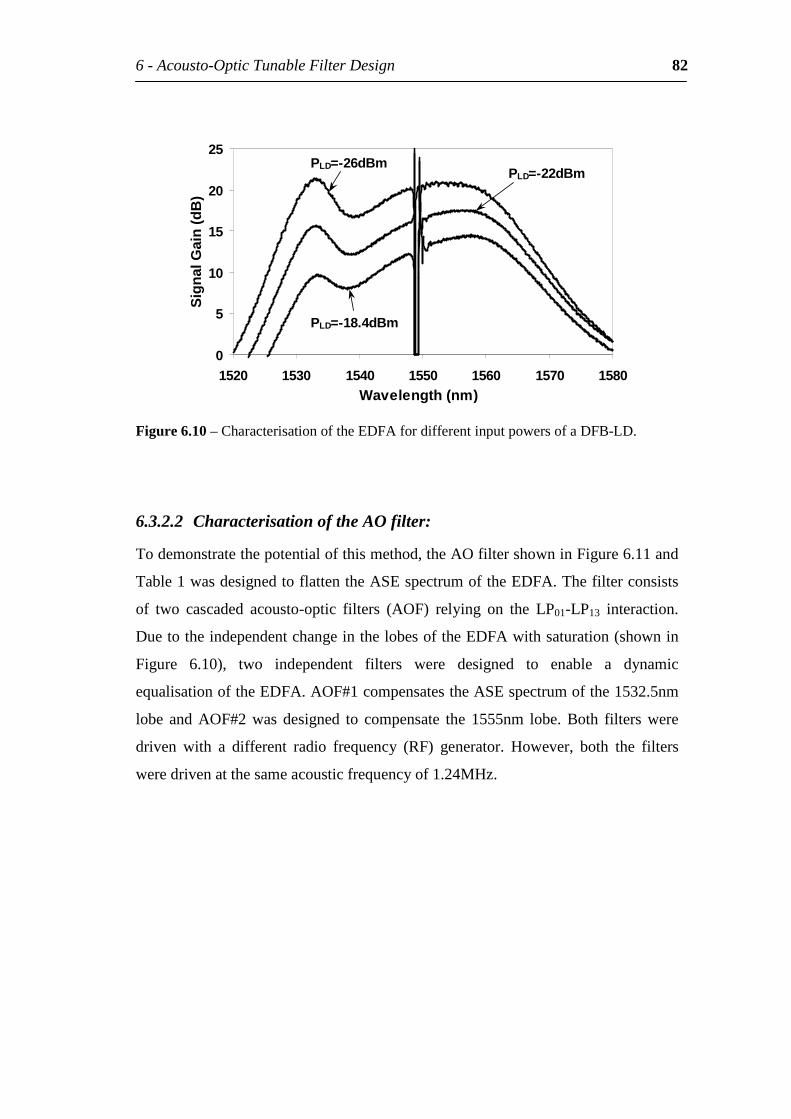
6-Acousto-OpticTunableFilterDesign 82
0
5
10
15
20
25
1520 1530 1540 1550 1560 1570 1580Wavelength(nm)
Sig
nalG
ain
(dB
)
PLD=-26dBmPLD=-22dBm
PLD=-18.4dBm
Figure6.10–CharacterisationoftheEDFAfordifferentinputpowersofaDFB-LD.
6.3.2.2 CharacterisationoftheAOfilter:
Todemonstratethepotentialofthismethod,theAOfiltershowninFigure6.11and
Table1wasdesignedtoflattentheASEspectrumoftheEDFA.Thefilterconsists
of two cascaded acousto-optic filters (AOF) relying on the LP01-LP13 interaction.
DuetotheindependentchangeinthelobesoftheEDFAwithsaturation(shownin
Figure 6.10), two independent filters were designed to enable a dynamic
equalisationoftheEDFA.AOF#1compensatestheASEspectrumofthe1532.5nm
lobe and AOF#2 was designed to compensate the 1555nm lobe. Both filters were
driven with a different radio frequency (RF) generator. However, both the filters
weredrivenatthesameacousticfrequencyof1.24MHz.
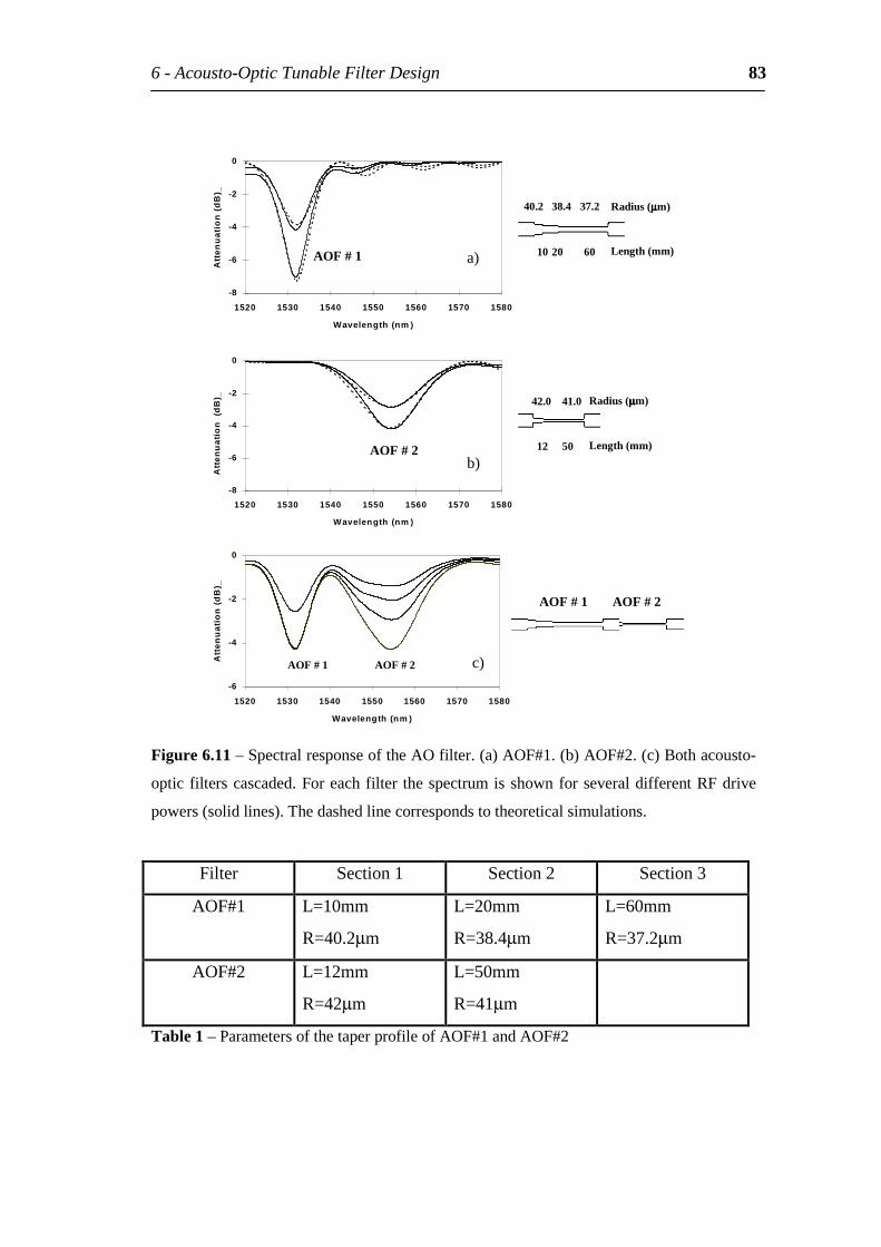
6-Acousto-OpticTunableFilterDesign 83
10 20 60 Length(mm)
40.2 38.4 37.2 Radius(µµµµm)
12 50 Length(mm)
42.0 41.0 Radius(µµµµm)
-6
-4
-2
0
1520 1530 1540 1550 1560 1570 1580
Wavelength(nm )
Att
enu
atio
n(
dB
)_
-8
-6
-4
-2
0
1520 1530 1540 1550 1560 1570 1580
Wavelength(nm )
Att
en
ua
tio
n
(dB
)_
-8
-6
-4
-2
0
1520 1530 1540 1550 1560 1570 1580
Wavelength(nm )
Att
enu
atio
n(
dB
)_
a)
b)
AOF#2AOF#1 c)
AOF#1
AOF#2
AOF#1 AOF#2
Figure6.11–SpectralresponseoftheAOfilter.(a)AOF#1.(b)AOF#2.(c)Bothacousto-
optic filterscascaded.Foreachfilter thespectrumisshownforseveraldifferentRFdrive
powers(solidlines).Thedashedlinecorrespondstotheoreticalsimulations.
Filter Section1 Section2 Section3
AOF#1 L=10mm
R=40.2µm
L=20mm
R=38.4µm
L=60mm
R=37.2µm
AOF#2 L=12mm
R=42µm
L=50mm
R=41µm
Table1–ParametersofthetaperprofileofAOF#1andAOF#2
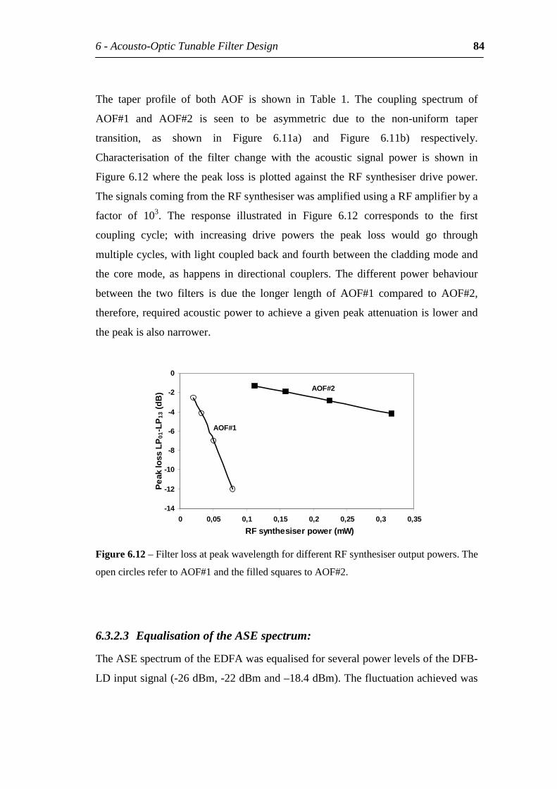
6-Acousto-OpticTunableFilterDesign 84
The taper profile of both AOF is shown in Table 1. The coupling spectrum of
AOF#1 and AOF#2 is seen to be asymmetric due to the non-uniform taper
transition, as shown in Figure 6.11a) and Figure 6.11b) respectively.
Characterisation of the filter change with the acoustic signal power is shown in
Figure6.12where thepeak loss isplottedagainst theRFsynthesiserdrivepower.
ThesignalscomingfromtheRFsynthesiserwasamplifiedusingaRFamplifierbya
factor of 103. The response illustrated in Figure 6.12 corresponds to the first
coupling cycle; with increasing drive powers the peak loss would go through
multiplecycles,withlightcoupledbackandfourthbetweenthecladdingmodeand
the core mode, as happens in directional couplers. The different power behaviour
between the two filters is due the longer length of AOF#1 compared to AOF#2,
therefore,requiredacousticpowertoachieveagivenpeakattenuationislowerand
thepeakisalsonarrower.
-14
-12
-10
-8
-6
-4
-2
0
0 0,05 0,1 0,15 0,2 0,25 0,3 0,35
RFsynthesiserpower(mW)
Pea
klo
ssL
P01
-LP
13(d
B)
AOF#1
AOF#2
Figure6.12–FilterlossatpeakwavelengthfordifferentRFsynthesiseroutputpowers.The
opencirclesrefertoAOF#1andthefilledsquarestoAOF#2.
6.3.2.3 EqualisationoftheASEspectrum:
TheASEspectrumoftheEDFAwasequalisedforseveralpowerlevelsoftheDFB-
LDinputsignal(-26dBm,-22dBmand–18.4dBm).Thefluctuationachievedwas
6-Acousto-OpticTunableFilterDesign 85
lessthan1dBforabandwidthofover30nmforallsaturationlevels.TheAOfilter
was tunedby changing only the electricpowersused todrive the acousticwaves.
TheexperimentalresultsobtainedarepresentedinFigure6.13.Theinsertionlossof
thewholefilterwasestimatedtobeless than0.5dB.Thetimeresponseof theAO
filter depends on the length of the device and the group velocity of the acoustic
flexuralwaveandisestimatedtobearound50µs.Thetotalpowerconsumptionof
thefilterwas1W.Thisvaluedidnotcorrespondtotherealcapabilitiesofthefilter
duetoanimpedancemismatchoftheamplifierwiththepiezoelectricelement.The
power consumption for an optimum efficiency is estimated to be of a several of
hundredsofmilliWatts.
TheprocessoftuningthisAOfilterismuchsimplercomparedtoothermulti-
frequency schemes. The filter is tuned by changing only the acoustic wave
amplitudes.Thefilter’ slossspectrumshapeisfixedbythetailoredtaperprofileand
isnotable to react toseverechanges in theamplifiergainspectrum(eachfilter is
designed for a specific amplifier). Reducing the tuning parameters increased the
facility of implementation and tuning the AO filter but, as a compromise, the
flexibility of the filter to accommodate to changes in the amplifier gain spectrum
wasalsoreducedincomparisontopreviousconfigurations.Forincreasedflexibility,
andstillasmallnumberoftuningparameters,thefrequencyoftheacousticwaveof
eachoftheindividualfilterscouldalsobetunedtoachievebetterequalisation.
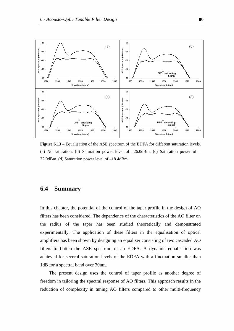
6-Acousto-OpticTunableFilterDesign 86
-30
-25
-20
-15
-10
1520 1530 1540 1550 1560 1570 1580
W avelength(nm)
AS
ES
pec
tru
m(
dB
m/n
m) (b)
-30
-25
-20
-15
-10
1520 1530 1540 1550 1560 1570 1580
W avelength(nm)
AS
ES
pec
tru
m(
dB
m/n
m) (c)
-30
-25
-20
-15
-10
1520 1530 1540 1550 1560 1570 1580
W avelength(nm)
AS
ES
pec
tru
m(
dB
m/n
m) (d)
-30
-25
-20
-15
-10
1520 1530 1540 1550 1560 1570 1580
Wavelength(nm)
AS
ES
pec
tru
m(
dB
m/n
m) (a)
DFBsaturatingSignal
DFBsaturatingSignal
DFBsaturatingSignal
Figure6.13–EqualisationoftheASEspectrumoftheEDFAfordifferentsaturationlevels.
(a) No saturation. (b) Saturation power level of –26.0dBm. (c) Saturation power of –
22.0dBm.(d)Saturationpowerlevelof–18.4dBm.
6.4 Summary
Inthischapter,thepotentialofthecontrolofthetaperprofileinthedesignofAO
filtershasbeenconsidered.ThedependenceofthecharacteristicsoftheAOfilteron
the radius of the taper has been studied theoretically and demonstrated
experimentally. The application of these filters in the equalisation of optical
amplifiershasbeenshownbydesigninganequaliserconsistingoftwocascadedAO
filters to flatten the ASE spectrum of an EDFA. A dynamic equalisation was
achieved for several saturation levelsof theEDFAwitha fluctuationsmaller than
1dBforaspectralbandover30nm.
The present design uses the control of taper profile as another degree of
freedomintailoringthespectralresponseofAOfilters.Thisapproachresultsinthe
reduction of complexity in tuning AO filters compared to other multi-frequency

6-Acousto-OpticTunableFilterDesign 87
schemes [16, 17, 26, 98]. However the flexibility of this design is limited to the
shapeofthefiltergivenbythecomplextaperprofile.Combiningbothtechniquesby
the use of several driving acoustic frequencies may allow the use of a minimum
numberofparameterstotunetheAOfilterdynamically.
7
IdealFilterDesignfor
EDFAGainEqualisation
The design of ideal filters to equalise the EDFA gain spectrum is studied using
differentconfigurations.Filtersbasedonanidealwavelength-dependentbackground
lossoftheEDFarepresentedandcomparedwithlumpedfiltersbasedontheinverse
of theamplifiergainspectrum.Special filtersaredesigned inorder tocompensate
for their own insertion losses giving no penalty to the amplifier gain and gain
flatness. With these novel filter designs EDFA equalisation is achieved with no
penaltyintheamplifiergainforinsertionlossesupto8dB.
7-IdealFilterDesignforEDFAGainEqualisation 89
7.1 Introduction
Erbium-doped fibre amplifiers (EDFA) play an important role in wavelength
divisionmultiplexing(WDM)systems.Asthenumberofchannelsinthesesystems
increases, broadband and equalised amplification is required. Several methods of
achievingEDFAequalisation,eitherintrinsicorextrinsic,havebeenproposedinthe
literatureasmentionedpreviouslyinsection2.5.Thesedeviceshavecharacteristic
equalisationpropertiesandinsertionlossesthatcouldbeaslowasthesplicingloss
betweentheEDFfibreandthefilterfibreandashigh8-9dB[24,25].
H. Zech reported a study of a theoretical filter to flatten the EDFA gain
spectrumacrossadesiredbandwidth.Thefilterisproposedintheformofanideal
wavelength-dependent background loss along the EDF length [104]. However, a
practicalimplementationofthistypeoffilteralongtheEDFlengthisverydifficult.
Inthischapter,theinitialtheoryisextendedtocalculatetheidealwavelength-
dependentbackgroundlossbyincludingthefibrebackgroundlosstermoftheEDF.
In the case of a lossy fibre, the ideal filter shape given by Zech [104] should be
corrected to incorporate this wavelength-independent fibre background loss. The
practicalimplementationofthedistributedbackgroundlossbyintegratingitintoone
ortwofiltersinsertedatdifferentpositionsalongtheamplifierisalsostudied.The
optimum placement of these filters within the EDFA is calculated both for a
configuration using one filter and two filters to equalise the gain spectrum.
Furthermore, the incorporation of the filter insertion loss in the filter design is
achievedbytreatingitasawavelength-independentdistributedlossandcorrecting
the filter design for this loss. With this correction, the filter insertion loss can be
compensatedforbyanefficientfilterre-designandoptimumpositioningwithinthe
EDFA. This is especially important for filters with high insertion losses, which
couldgoupto8-9dB[24,25].
7-IdealFilterDesignforEDFAGainEqualisation 90
7.1.1 TheoreticalModel
Inthisworkaspectralmodel[11]isusedtodescribetheamplifierperformance.The
spatialcharacteristicsoftheEDFareintegratedandtherateequationsareexpressed
asinChapter2.ThemodelisbasedontheknowledgeoftheEDFparametersα(λ),
g*(λ), l(λ) and the ratio of the linear density of erbium ions to the fluorescence
lifetime ξ(λ). Several methods have been studied in the literature to measure the
amplifierlossandgainspectra[105-107].Theα(λ)andg*(λ)usedinthenumerical
simulationsweremeasuredfromareal fibreandare illustrated inFigure2.3,with
ξ=4.7x10¹⁵m-1s-1and lBG=4.9dB/kmat1200nm.Theinputsignalwasdividedinto
32 channels on a 100GHz grid from 1532nm to 1557nm. The calculations were
performedby running the rateequations (2.4)and (2.5)backand fourth along the
amplifierlengthuntilalltheparametersmetthegivenconvergencecriteria(shooting
method).The forwardamplified spontaneous emission (ASE)was fixed tozero at
thebeginingoftheamplifierandthebackwardASEwasfixedtozeroattheendof
theamplifier.Thenumericalsimulationsshowthattheconvergenceoftheamplifier
structureisachievedafterafewiterations.
7.2 Theoreticalfilterdesign:
According to Zech [104], in order to equalise the EDFA gain spectrum, an ideal
distributedloss,canbedeterminedanalyticallyifthewavelengthdependenceofthe
modefunctions in thesignal range isneglected.This isa fairassumptionover the
limited C and L EDFA bands. In this case, the spontaneous emission term is
neglectedandtherateequationforthesignalpowercanbewrittenintheform[11]:
( )( )
)(
)()(
2
tkkk
kkkk
nn
zPg
zPldz
zdP
=+
++
α
α (7.1)
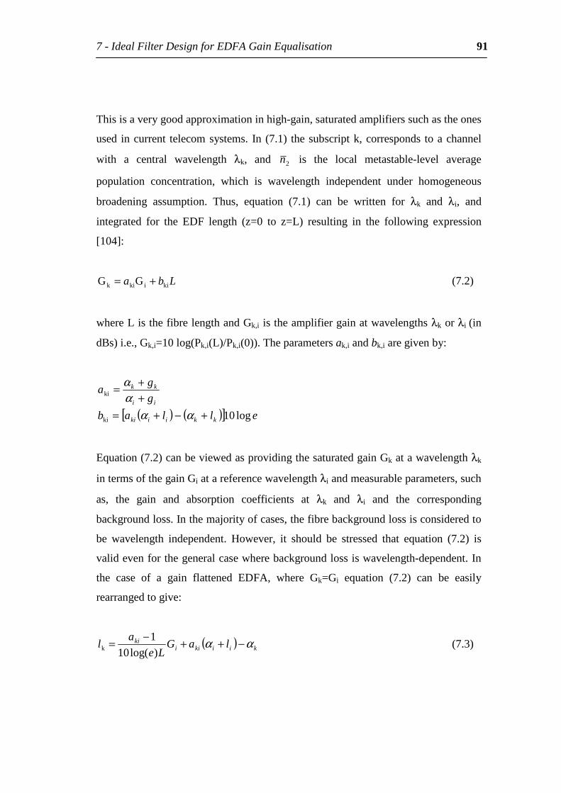
7-IdealFilterDesignforEDFAGainEqualisation 91
Thisisaverygoodapproximationinhigh-gain,saturatedamplifierssuchastheones
used incurrent telecomsystems. In (7.1) thesubscriptk,corresponds toachannel
with a central wavelength λk, and 2n is the local metastable-level average
population concentration, which is wavelength independent under homogeneous
broadening assumption. Thus, equation (7.1) can be written for λk and λi, and
integrated for the EDF length (z=0 to z=L) resulting in the following expression
[104]:
Lba kiikik GG += (7.2)
whereListhefibrelengthandGk,iistheamplifiergainatwavelengthsλkorλi(in
dBs)i.e.,Gk,i=10log(Pk,i(L)/Pk,i(0)).Theparametersak,iandbk,iaregivenby:
( ) ( )[ ] ellab
gg
a
kkiiki
ii
kk
log10ki
ki
+−+=++=
αααα
Equation(7.2)canbeviewedasprovidingthesaturatedgainGkatawavelengthλk
intermsofthegainGiatareferencewavelengthλiandmeasurableparameters,such
as, the gain and absorption coefficients at λk and λi and the corresponding
backgroundloss.Inthemajorityofcases,thefibrebackgroundlossisconsideredto
be wavelength independent. However, it should be stressed that equation (7.2) is
validevenforthegeneralcasewherebackgroundlossiswavelength-dependent.In
the case of a gain flattened EDFA, where Gk=Gi equation (7.2) can be easily
rearrangedtogive:
( ) kiikiiki laG
Lea
l αα −++−=)log(10
1k (7.3)
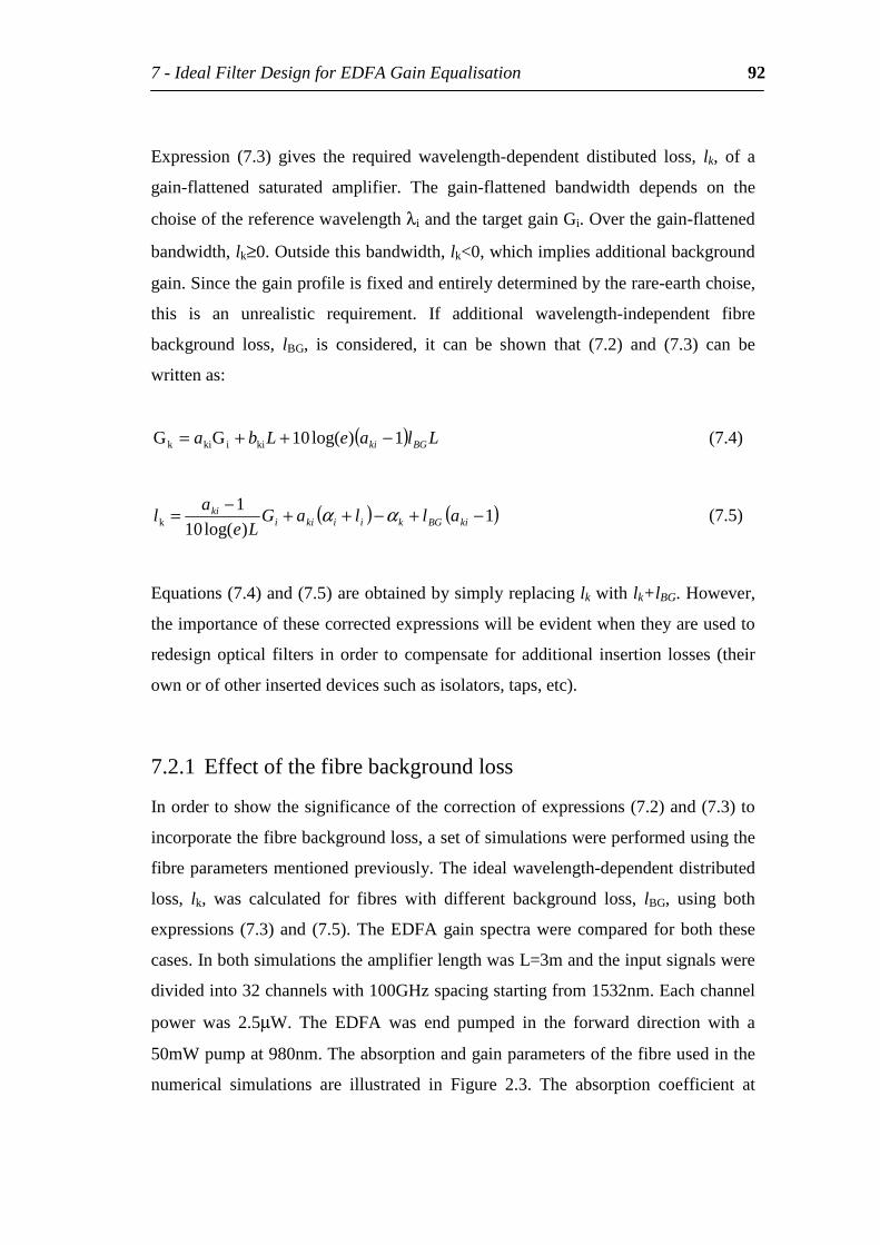
7-IdealFilterDesignforEDFAGainEqualisation 92
Expression (7.3) gives the required wavelength-dependent distibuted loss, lk, of a
gain-flattened saturated amplifier. The gain-flattened bandwidth depends on the
choiseofthereferencewavelengthλiandthetargetgainGi.Overthegain-flattened
bandwidth,lk≥0.Outsidethisbandwidth,lk<0,whichimpliesadditionalbackground
gain.Sincethegainprofileisfixedandentirelydeterminedbytherare-earthchoise,
this is an unrealistic requirement. If additional wavelength-independent fibre
background loss, lBG, is considered, it can be shown that (7.2) and (7.3) can be
writtenas:
( ) LlaeLba BGki 1)log(10GG kiikik −++= (7.4)
( ) ( )1)log(10
1k −+−++−= kiBGkiikii
ki allaGLe
al αα (7.5)
Equations(7.4)and(7.5)areobtainedbysimplyreplacinglkwithlk+lBG.However,
theimportanceofthesecorrectedexpressionswillbeevidentwhentheyareusedto
redesignoptical filters inorder to compensate foradditional insertion losses (their
ownorofotherinserteddevicessuchasisolators,taps,etc).
7.2.1 Effectofthefibrebackgroundloss
Inordertoshowthesignificanceofthecorrectionofexpressions(7.2)and(7.3)to
incorporatethefibrebackgroundloss,asetofsimulationswereperformedusingthe
fibreparametersmentionedpreviously.Theidealwavelength-dependentdistributed
loss, lk, was calculated for fibres with different background loss, lBG, using both
expressions(7.3)and(7.5).TheEDFAgainspectrawerecomparedforboth these
cases.InbothsimulationstheamplifierlengthwasL=3mandtheinputsignalswere
dividedinto32channelswith100GHzspacingstartingfrom1532nm.Eachchannel
power was 2.5µW. The EDFA was end pumped in the forward direction with a
50mWpumpat980nm.Theabsorptionandgainparametersofthefibreusedinthe
numerical simulations are illustrated in Figure 2.3. The absorption coefficient at
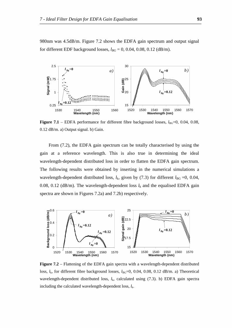
7-IdealFilterDesignforEDFAGainEqualisation 93
980nmwas4.5dB/m.Figure7.2showstheEDFAgainspectrumandoutputsignal
fordifferentEDFbackgroundlosses,lBG=0,0.04,0.08,0.12(dB/m).
0.25
1
1.75
2.5
1530 1540 1550 1560Wavelength(nm)
Sig
nal
(m
W)
a)l Bg =0
l Bg =0.1215
20
25
30
1520 1530 1540 1550 1560 1570Wavelength(nm)
Gai
n(d
B)
b)l Bg =0
l Bg =0.12
Figure 7.1 – EDFA performance fordifferent fibrebackground losses, lBG=0, 0.04, 0.08,
0.12dB/m.a)Outputsignal.b)Gain.
From(7.2), theEDFAgainspectrumcanbetotallycharacterisedbyusingthe
gain at a reference wavelength. This is also true in determining the ideal
wavelength-dependentdistributed loss inorder to flatten theEDFAgainspectrum.
The following results were obtained by inserting in the numerical simulations a
wavelength-dependentdistributed loss, lk,givenby(7.3) fordifferent lBG=0,0.04,
0.08,0.12(dB/m).Thewavelength-dependentlosslkandtheequalisedEDFAgain
spectraareshowninFigures7.2a)and7.2b)respectively.
0
0.2
0.4
0.6
1520 1530 1540 1550 1560 1570Wavelength(nm)
Bac
kgro
un
dlo
ss(
dB
/m)
a)
l Bg =0.12
l Bg =0
l Bg =0.12
l Bg =0
15
17.5
20
22.5
25
1520 1530 1540 1550 1560 1570Wavelength(nm)
Sig
nal
gai
n(
dB) b)
l Bg =0.12
l Bg =0
Figure7.2–FlatteningoftheEDFAgainspectrawithawavelength-dependentdistributed
loss, lk, fordifferent fibrebackground losses, lBG=0,0.04,0.08,0.12dB/m.a)Theoretical
wavelength-dependent distributed loss, lk, calculated using (7.3). b) EDFA gain spectra
includingthecalculatedwavelength-dependentloss,lk.
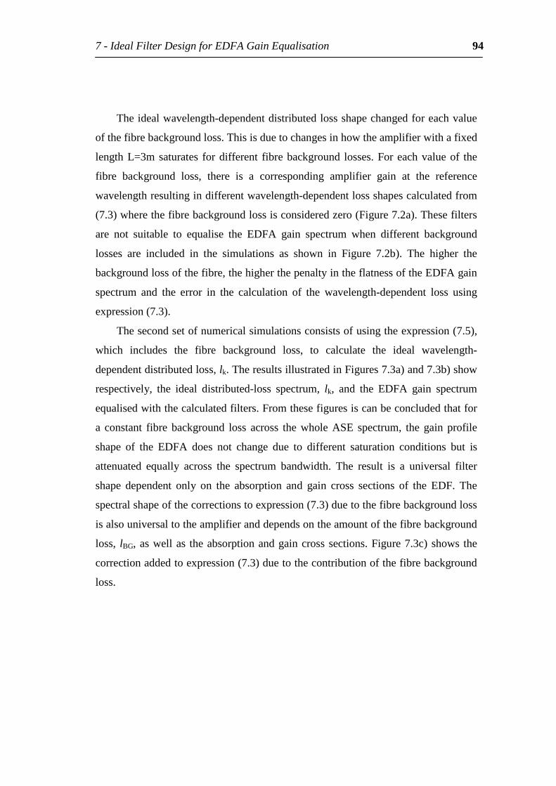
7-IdealFilterDesignforEDFAGainEqualisation 94
Theidealwavelength-dependentdistributedlossshapechangedforeachvalue
ofthefibrebackgroundloss.Thisisduetochangesinhowtheamplifierwithafixed
lengthL=3msaturates fordifferent fibrebackground losses.Foreachvalueof the
fibre background loss, there is a corresponding amplifier gain at the reference
wavelengthresultingindifferentwavelength-dependentlossshapescalculatedfrom
(7.3)wherethefibrebackgroundlossisconsideredzero(Figure7.2a).Thesefilters
are not suitable to equalise the EDFA gain spectrum when different background
losses are included in the simulations as shown in Figure 7.2b). The higher the
backgroundlossofthefibre,thehigherthepenaltyintheflatnessoftheEDFAgain
spectrum and the error in the calculation of the wavelength-dependent loss using
expression(7.3).
Thesecondsetofnumericalsimulationsconsistsofusingtheexpression(7.5),
which includes the fibre background loss, to calculate the ideal wavelength-
dependentdistributedloss,lk.TheresultsillustratedinFigures7.3a)and7.3b)show
respectively, the ideal distributed-loss spectrum, lk, and the EDFA gain spectrum
equalisedwiththecalculatedfilters.Fromthesefiguresiscanbeconcludedthatfor
a constant fibre background loss across the whole ASE spectrum, the gain profile
shape of the EDFA does not change due to different saturation conditions but is
attenuated equally across the spectrum bandwidth. The result is a universal filter
shape dependent only on the absorption and gain cross sections of the EDF. The
spectralshapeofthecorrectionstoexpression(7.3)duetothefibrebackgroundloss
isalsouniversaltotheamplifieranddependsontheamountofthefibrebackground
loss, lBG,aswellas theabsorptionandgaincrosssections.Figure7.3c) shows the
correctionaddedtoexpression(7.3)duetothecontributionofthefibrebackground
loss.
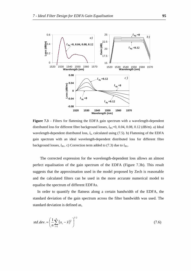
7-IdealFilterDesignforEDFAGainEqualisation 95
0
0.2
0.4
0.6
1520 1530 1540 1550 1560 1570Wavelength(nm)
Loss
(dB
/m)
a)
l Bg =0,0.04,0.08,0.12
15
17.5
20
22.5
25
1520 1530 1540 1550 1560 1570Wavelength(nm)
Gai
n(d
B)
b)
l Bg =0.12
l Bg =0
-0.08
-0.04
0
0.04
0.08
1520 1530 1540 1550 1560 1570Wavelength(nm)
Loss
(dB
/m)
c)l Bg =0.12
l Bg =0l Bg =0.12
l Bg =0
Figure7.3–Filters for flattening theEDFAgain spectrumwith awavelength-dependent
distributedlossfordifferentfibrebackgroundlosses,lBG=0,0.04,0.08,0.12(dB/m).a)Ideal
wavelength-dependentdistributedloss,lk,calculatedusing(7.5).b)FlatteningoftheEDFA
gain spectrum with an ideal wavelength-dependent distributed loss for different fibre
backgroundlosses,lBG.c)Correctiontermaddedto(7.3)duetolBG.
The corrected expression for thewavelength-dependent loss allowsan almost
perfect equalisation of the gain spectrum of the EDFA (Figure 7.3b). This result
suggests that theapproximationused inthemodelproposedbyZech is reasonable
and the calculated filters can be used in the more accurate numerical model to
equalisethespectrumofdifferentEDFAs.
In order to quantify the flatness along a certain bandwidth of the EDFA, the
standarddeviationof thegain spectrumacross the filter bandwidthwasused.The
standarddeviationisdefinedas,
( )2/1
1
21..
−= =
n
ii xx
ndevstd (7.6)
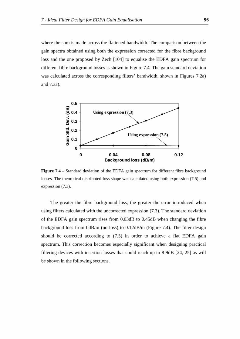
7-IdealFilterDesignforEDFAGainEqualisation 96
wherethesumismadeacrosstheflattenedbandwidth.Thecomparisonbetweenthe
gainspectraobtainedusingboth theexpressioncorrectedfor thefibrebackground
lossand theoneproposedbyZech [104] toequalise theEDFAgain spectrumfor
differentfibrebackgroundlossesisshowninFigure7.4.Thegainstandarddeviation
wascalculatedacrossthecorrespondingfilters’ bandwidth,showninFigures7.2a)
and7.3a).
0
0.1
0.2
0.3
0.4
0.5
0 0.04 0.08 0.12Backgroundloss(dB/m)
Gai
nS
td.D
ev.(
dB)
Usingexpression(7.3)
Usingexpression(7.5)
Figure7.4–StandarddeviationoftheEDFAgainspectrumfordifferentfibrebackground
losses.Thetheoreticaldistributed-lossshapewascalculatedusingbothexpression(7.5)and
expression(7.3).
The greater the fibre background loss, the greater the error introduced when
usingfilterscalculatedwiththeuncorrectedexpression(7.3).Thestandarddeviation
of theEDFAgain spectrumrises from0.03dB to0.45dBwhenchanging the fibre
background loss from0dB/m(no loss) to0.12dB/m(Figure7.4).The filterdesign
should be corrected according to (7.5) in order to achieve a flat EDFA gain
spectrum. This correction becomes especially significant when designing practical
filteringdeviceswithinsertionlossesthatcouldreachupto8-9dB[24,25]aswill
beshowninthefollowingsections.
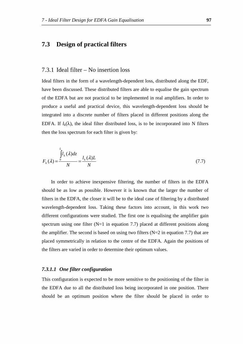
7-IdealFilterDesignforEDFAGainEqualisation 97
7.3 Designofpracticalfilters
7.3.1 Idealfilter–Noinsertionloss
Idealfiltersintheformofawavelength-dependentloss,distributedalongtheEDF,
havebeendiscussed.Thesedistributedfiltersareabletoequalisethegainspectrum
oftheEDFAbutarenotpracticaltobeimplementedinrealamplifiers.Inorderto
produce a useful and practical device, this wavelength-dependent loss should be
integrated into a discrete number of filters placed in different positions along the
EDFA. If lk(λ), the ideal filter distributed loss, is tobe incorporated intoN filters
thenthelossspectrumforeachfilterisgivenby:
NLl
N
dzl
F k
L
k
k
)()(
)( 0 λλ
λ ==
(7.7)
In order to achieve inexpensive filtering, the number of filters in the EDFA
should be as low as possible. However it is known that the larger the number of
filtersintheEDFA,thecloseritwillbetotheidealcaseoffilteringbyadistributed
wavelength-dependent loss. Taking these factors into account, in this work two
differentconfigurationswerestudied.Thefirstoneisequalisingtheamplifiergain
spectrumusingone filter (N=1 inequation7.7)placedatdifferentpositionsalong
theamplifier.Thesecondisbasedonusingtwofilters(N=2inequation7.7)thatare
placedsymmetricallyinrelationtothecentreof theEDFA.Againthepositionsof
thefiltersarevariedinordertodeterminetheiroptimumvalues.
7.3.1.1 Onefilterconfiguration
Thisconfigurationisexpectedtobemoresensitivetothepositioningofthefilterin
theEDFAdue toall thedistributed lossbeing incorporated inoneposition.There
should be an optimum position where the filter should be placed in order to
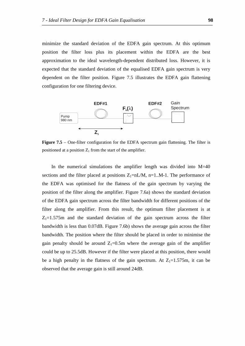
7-IdealFilterDesignforEDFAGainEqualisation 98
minimize the standard deviation of the EDFA gain spectrum. At this optimum
position the filter loss plus its placement within the EDFA are the best
approximation to the ideal wavelength-dependent distributed loss. However, it is
expected that the standarddeviationof theequalisedEDFAgain spectrum isvery
dependent on the filter position. Figure 7.5 illustrates the EDFA gain flattening
configurationforonefilteringdevice.
Pump980nm
Z1
EDF#1 EDF#2F ( )k λ
GainSpectrum
Figure7.5–One-filterconfigurationfortheEDFAspectrumgainflattening.Thefilter is
positionedatapositionZ1fromthestartoftheamplifier.
In the numerical simulations the amplifier length was divided into M=40
sectionsandthefilterplacedatpositionsZ1=nL/M,n=1..M-1.Theperformanceof
the EDFA was optimised for the flatness of the gain spectrum by varying the
positionofthefilteralongtheamplifier.Figure7.6a)showsthestandarddeviation
oftheEDFAgainspectrumacrossthefilterbandwidthfordifferentpositionsofthe
filter along the amplifier. From this result, the optimum filter placement is at
Z1=1.575m and the standard deviation of the gain spectrum across the filter
bandwidthislessthan0.07dB.Figure7.6b)showstheaveragegainacrossthefilter
bandwidth.Thepositionwherethefiltershouldbeplacedinordertominimisethe
gain penalty should be around Z1=0.5m where the average gain of the amplifier
couldbeupto25.5dB.Howeverifthefilterwereplacedatthisposition,therewould
be a high penalty in the flatness of the gain spectrum. At Z1=1.575m, it can be
observedthattheaveragegainisstillaround24dB.
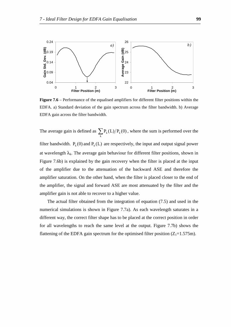
7-IdealFilterDesignforEDFAGainEqualisation 99
0.04
0.09
0.14
0.19
0.24
0 1 2 3FilterPosition(m)
Gai
nS
td.D
ev.(
dB) a)
22
23
24
25
26
0 1 2 3FilterPosition(m)
Ave
rage
Gai
n(d
B)
b)
Figure7.6–Performanceoftheequalisedamplifiersfordifferentfilterpositionswithinthe
EDFA.a)Standarddeviationofthegainspectrumacrossthefilterbandwidth.b)Average
EDFAgainacrossthefilterbandwidth.
Theaveragegainisdefinedask
kk )0(P)L(P ,wherethesumisperformedoverthe
filterbandwidth. )L(Pand)0(P kk arerespectively,theinputandoutputsignalpower
atwavelengthλk.Theaveragegainbehaviourfordifferentfilterpositions,shownin
Figure7.6b)isexplainedbythegainrecoverywhenthefilterisplacedattheinput
of the amplifier due to the attenuation of the backward ASE and therefore the
amplifiersaturation.Ontheotherhand,whenthefilterisplacedclosertotheendof
theamplifier,thesignalandforwardASEaremostattenuatedbythefilterandthe
amplifiergainisnotabletorecovertoahighervalue.
Theactualfilterobtainedfromtheintegrationofequation(7.5)andusedinthe
numericalsimulations isshowninFigure7.7a).Aseachwavelengthsaturates ina
differentway,thecorrectfiltershapehastobeplacedatthecorrectpositioninorder
for all wavelengths to reach the same level at the output. Figure 7.7b) shows the
flatteningoftheEDFAgainspectrumfortheoptimisedfilterposition(Z1=1.575m).
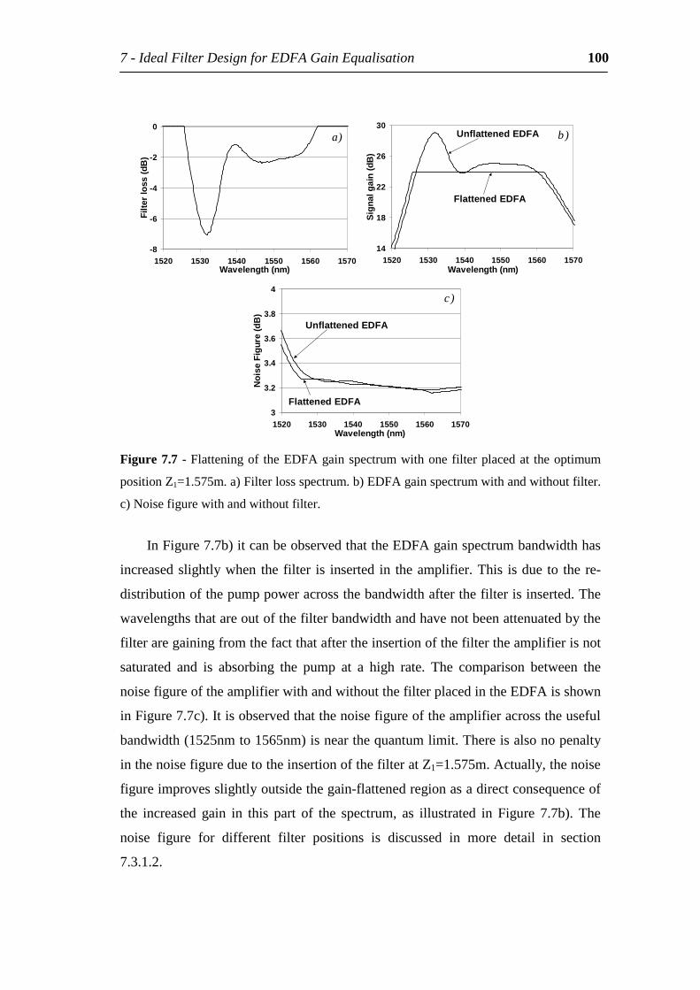
7-IdealFilterDesignforEDFAGainEqualisation 100
-8
-6
-4
-2
0
1520 1530 1540 1550 1560 1570Wavelength(nm)
Filte
rlo
ss(d
B)
a)
14
18
22
26
30
1520 1530 1540 1550 1560 1570Wavelength(nm)
Sig
nalg
ain
(dB
)
b)UnflattenedEDFA
FlattenedEDFA
3
3.2
3.4
3.6
3.8
4
1520 1530 1540 1550 1560 1570Wavelength(nm)
Noi
seF
igur
e(d
B)
c)
UnflattenedEDFA
FlattenedEDFA
Figure7.7-Flatteningof theEDFAgainspectrumwithonefilterplacedat theoptimum
positionZ1=1.575m.a)Filterlossspectrum.b)EDFAgainspectrumwithandwithoutfilter.
c)Noisefigurewithandwithoutfilter.
InFigure7.7b)itcanbeobservedthattheEDFAgainspectrumbandwidthhas
increasedslightlywhen thefilter is inserted in theamplifier.This isdue to there-
distributionofthepumppoweracrossthebandwidthafterthefilterisinserted.The
wavelengthsthatareoutofthefilterbandwidthandhavenotbeenattenuatedbythe
filteraregainingfromthefactthataftertheinsertionofthefiltertheamplifierisnot
saturated and is absorbing the pump at a high rate. The comparison between the
noisefigureoftheamplifierwithandwithoutthefilterplacedintheEDFAisshown
inFigure7.7c).Itisobservedthatthenoisefigureoftheamplifieracrosstheuseful
bandwidth(1525nmto1565nm)isnearthequantumlimit.Thereisalsonopenalty
inthenoisefigureduetotheinsertionofthefilteratZ1=1.575m.Actually,thenoise
figureimprovesslightlyoutsidethegain-flattenedregionasadirectconsequenceof
the increased gain in this part of the spectrum, as illustrated in Figure 7.7b). The
noise figure for different filter positions is discussed in more detail in section
7.3.1.2.
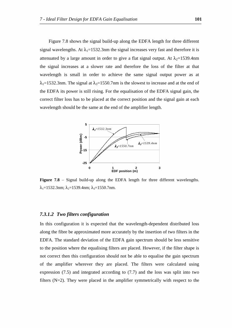
7-IdealFilterDesignforEDFAGainEqualisation 101
Figure7.8showsthesignalbuild-upalongtheEDFAlengthforthreedifferent
signalwavelengths.Atλ1=1532.3nmthesignalincreasesveryfastandthereforeitis
attenuatedbyalargeamountinordertogiveaflatsignaloutput.Atλ2=1539.4nm
the signal increases at a slower rate and therefore the loss of the filter at that
wavelength is small in order to achieve the same signal output power as at
λ1=1532.3nm.Thesignalatλ3=1550.7nmistheslowesttoincreaseandattheendof
theEDFAitspowerisstillrising.FortheequalisationoftheEDFAsignalgain,the
correctfilterlosshastobeplacedatthecorrectpositionandthesignalgainateach
wavelengthshouldbethesameattheendoftheamplifierlength.
-25
-15
-5
5
0 1 2 3EDFposition(m)
Po
wer
(dB
m)
λλλλ 3333=1550.7nm
λλλλ 1111=1532.3nm
λλλλ 2222=1539.4nm
Figure 7.8 – Signal build-up along the EDFA length for three different wavelengths.
λ1=1532.3nm;λ2=1539.4nm;λ3=1550.7nm.
7.3.1.2 Twofiltersconfiguration
In this configuration it is expected that the wavelength-dependent distributed loss
alongthefibrebeapproximatedmoreaccuratelybytheinsertionoftwofiltersinthe
EDFA.ThestandarddeviationoftheEDFAgainspectrumshouldbelesssensitive
tothepositionwheretheequalisingfiltersareplaced.However,ifthefiltershapeis
notcorrectthenthisconfigurationshouldnotbeabletoequalisethegainspectrum
of the amplifier wherever they are placed. The filters were calculated using
expression (7.5) and integrated according to (7.7) and the loss was split into two
filters (N=2).Theywereplaced in the amplifier symmetricallywith respect to the
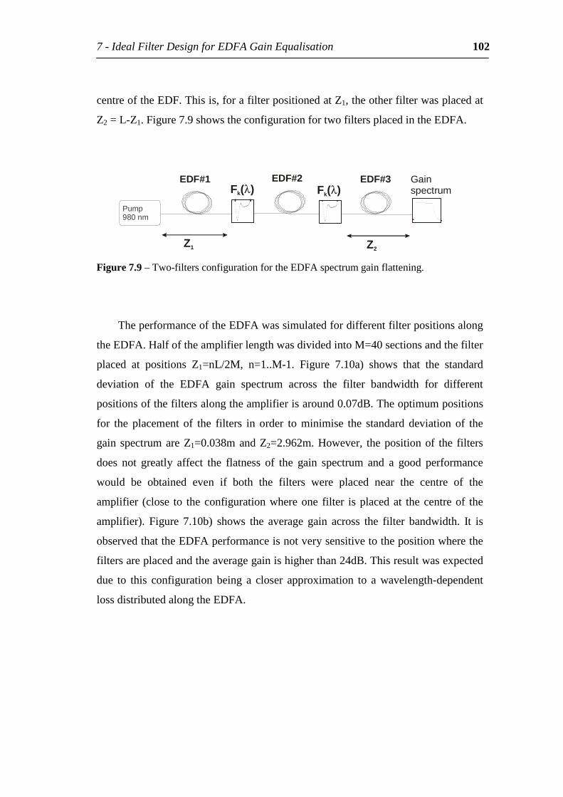
7-IdealFilterDesignforEDFAGainEqualisation 102
centreoftheEDF.Thisis,forafilterpositionedatZ1,theotherfilterwasplacedat
Z2=L-Z1.Figure7.9showstheconfigurationfortwofiltersplacedintheEDFA.
Pump980nm
Z1 Z2
EDF#1 EDF#2 EDF#3F ( )k λF ( )k λ
Gainspectrum
Figure7.9–Two-filtersconfigurationfortheEDFAspectrumgainflattening.
TheperformanceoftheEDFAwassimulatedfordifferentfilterpositionsalong
theEDFA.HalfoftheamplifierlengthwasdividedintoM=40sectionsandthefilter
placed at positions Z1=nL/2M, n=1..M-1. Figure 7.10a) shows that the standard
deviation of the EDFA gain spectrum across the filter bandwidth for different
positionsofthefiltersalongtheamplifierisaround0.07dB.Theoptimumpositions
for the placement of the filters in order to minimise the standard deviation of the
gain spectrumareZ1=0.038mandZ2=2.962m.However, thepositionof the filters
does not greatly affect the flatness of the gain spectrum and a good performance
would be obtained even if both the filters were placed near the centre of the
amplifier (close to the configurationwhereone filter isplacedat the centreof the
amplifier). Figure 7.10b) shows the average gain across the filter bandwidth. It is
observedthattheEDFAperformanceisnotverysensitivetothepositionwherethe
filtersareplacedandtheaveragegainishigherthan24dB.Thisresultwasexpected
due to this configuration being a closer approximation to a wavelength-dependent
lossdistributedalongtheEDFA.
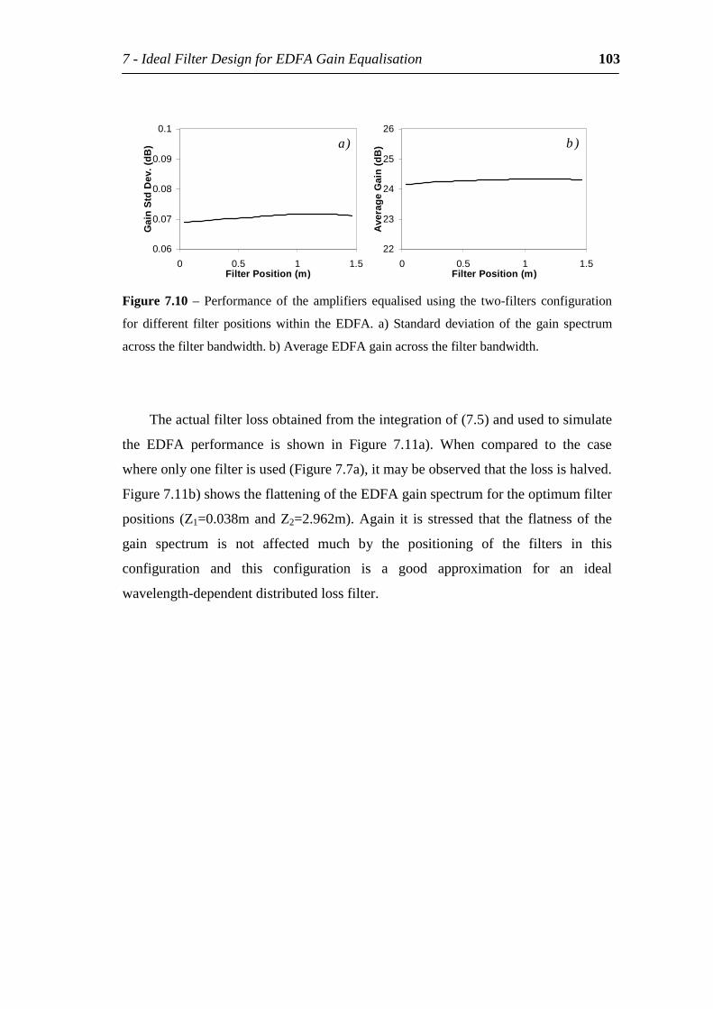
7-IdealFilterDesignforEDFAGainEqualisation 103
0.06
0.07
0.08
0.09
0.1
0 0.5 1 1.5FilterPosition(m)
Gai
nS
tdD
ev.(
dB) a)
22
23
24
25
26
0 0.5 1 1.5FilterPosition(m)
Ave
rage
Gai
n(d
B) b)
Figure7.10–Performanceof the amplifiers equalisedusing the two-filters configuration
fordifferent filter positionswithin theEDFA. a)Standarddeviationof thegain spectrum
acrossthefilterbandwidth.b)AverageEDFAgainacrossthefilterbandwidth.
Theactualfilterlossobtainedfromtheintegrationof(7.5)andusedtosimulate
the EDFA performance is shown in Figure 7.11a). When compared to the case
whereonlyonefilterisused(Figure7.7a),itmaybeobservedthatthelossishalved.
Figure7.11b)showstheflatteningoftheEDFAgainspectrumfortheoptimumfilter
positions (Z1=0.038mandZ2=2.962m).Again it is stressed that the flatnessof the
gain spectrum is not affected much by the positioning of the filters in this
configuration and this configuration is a good approximation for an ideal
wavelength-dependentdistributedlossfilter.
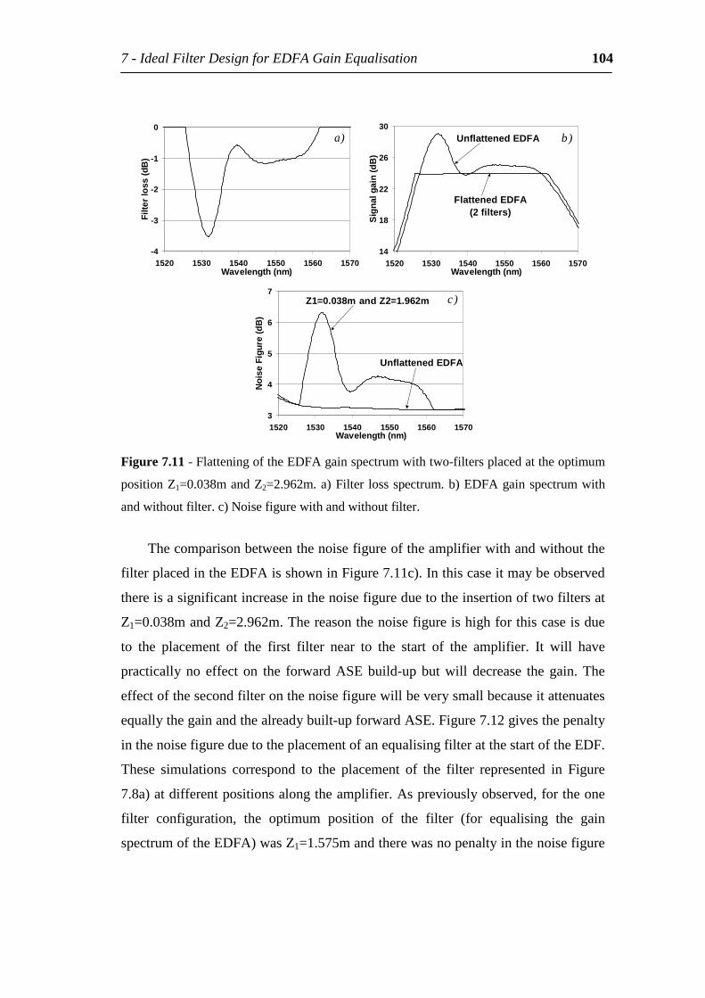
7-IdealFilterDesignforEDFAGainEqualisation 104
-4
-3
-2
-1
0
1520 1530 1540 1550 1560 1570Wavelength(nm)
Filte
rlo
ss(d
B)
a)
14
18
22
26
30
1520 1530 1540 1550 1560 1570Wavelength(nm)
Sig
nalg
ain
(dB
)
b)
FlattenedEDFA(2filters)
UnflattenedEDFA
3
4
5
6
7
1520 1530 1540 1550 1560 1570Wavelength(nm)
Noi
seF
igur
e(d
B)
c)Z1=0.038mandZ2=1.962m
UnflattenedEDFA
Figure7.11-FlatteningoftheEDFAgainspectrumwithtwo-filtersplacedattheoptimum
positionZ1=0.038mandZ2=2.962m.a)Filter lossspectrum.b)EDFAgainspectrumwith
andwithoutfilter.c)Noisefigurewithandwithoutfilter.
Thecomparisonbetweenthenoisefigureoftheamplifierwithandwithoutthe
filterplacedintheEDFAisshowninFigure7.11c).Inthiscaseitmaybeobserved
thereisasignificantincreaseinthenoisefigureduetotheinsertionoftwofiltersat
Z1=0.038mandZ2=2.962m.Thereasonthenoisefigureishighforthiscaseisdue
to the placement of the first filter near to the start of the amplifier. It will have
practicallyno effect on the forwardASEbuild-upbutwill decrease thegain.The
effectofthesecondfilteronthenoisefigurewillbeverysmallbecauseitattenuates
equallythegainandthealreadybuilt-upforwardASE.Figure7.12givesthepenalty
inthenoisefigureduetotheplacementofanequalisingfilteratthestartoftheEDF.
These simulations correspond to the placement of the filter represented in Figure
7.8a)atdifferentpositionsalongtheamplifier.Aspreviouslyobserved,fortheone
filter configuration, the optimum position of the filter (for equalising the gain
spectrumoftheEDFA)wasZ1=1.575mandtherewasnopenaltyinthenoisefigure
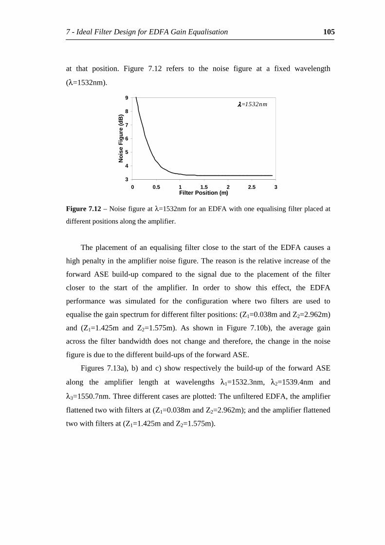
7-IdealFilterDesignforEDFAGainEqualisation 105
at that position. Figure 7.12 refers to the noise figure at a fixed wavelength
(λ=1532nm).
3
4
5
6
7
8
9
0 0.5 1 1.5 2 2.5 3FilterPosition(m)
Noi
seF
igur
e(d
B)
λλλλ=1532nm
Figure7.12–Noisefigureatλ=1532nmforanEDFAwithoneequalisingfilterplacedat
differentpositionsalongtheamplifier.
Theplacementof an equalising filter close to the start of theEDFAcauses a
highpenaltyintheamplifiernoisefigure.Thereasonistherelativeincreaseofthe
forward ASE build-up compared to the signal due to the placement of the filter
closer to the start of the amplifier. In order to show this effect, the EDFA
performance was simulated for the configuration where two filters are used to
equalisethegainspectrumfordifferentfilterpositions:(Z1=0.038mandZ2=2.962m)
and (Z1=1.425m and Z2=1.575m). As shown in Figure 7.10b), the average gain
across the filterbandwidthdoesnot changeand therefore, thechange in thenoise
figureisduetothedifferentbuild-upsoftheforwardASE.
Figures 7.13a), b) and c) show respectively the build-up of the forward ASE
along the amplifier length at wavelengths λ1=1532.3nm, λ2=1539.4nm and
λ3=1550.7nm.Threedifferentcasesareplotted:TheunfilteredEDFA,theamplifier
flattenedtwowithfiltersat(Z1=0.038mandZ2=2.962m);andtheamplifierflattened
twowithfiltersat(Z1=1.425mandZ2=1.575m).
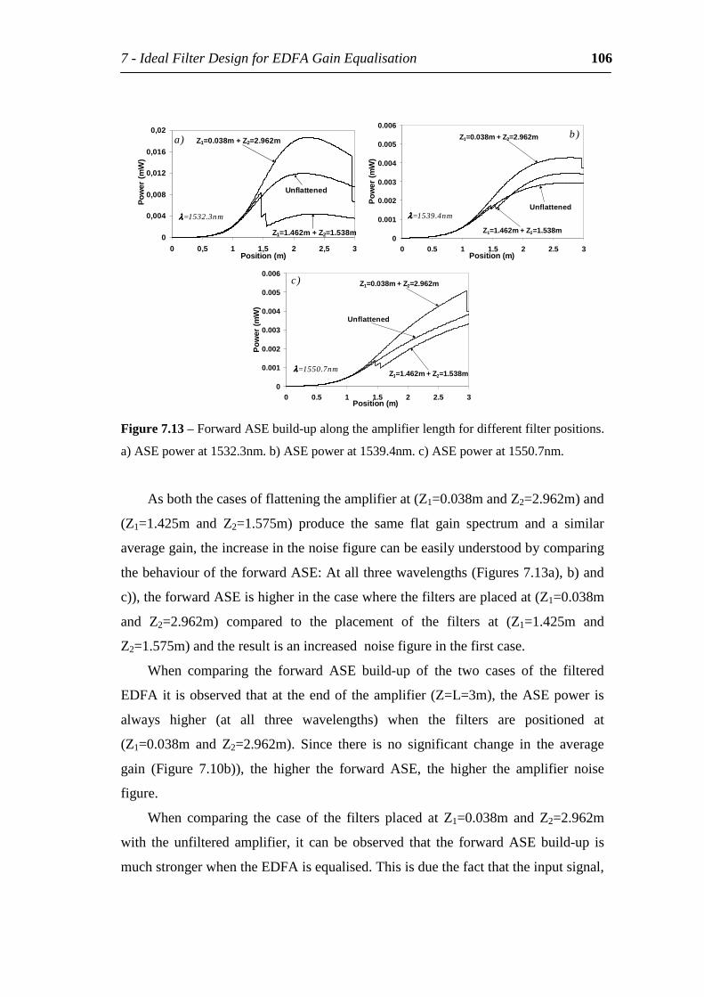
7-IdealFilterDesignforEDFAGainEqualisation 106
0
0,004
0,008
0,012
0,016
0,02
0 0,5 1 1,5 2 2,5 3Position(m)
Pow
er(
mW
)a) Z1=0.038m+Z2=2.962m
Z1=1.462m+Z2=1.538m
Unflattened
λλλλ=1532.3nm
0
0.001
0.002
0.003
0.004
0.005
0.006
0 0.5 1 1.5 2 2.5 3Position(m)
Pow
er(m
W)
b)Z1=0.038m+Z2=2.962m
Z1=1.462m+Z2=1.538m
Unflattenedλλλλ=1539.4nm
0
0.001
0.002
0.003
0.004
0.005
0.006
0 0.5 1 1.5 2 2.5 3Position(m)
Pow
er(m
W)
c) Z1=0.038m+Z2=2.962m
Z1=1.462m+Z2=1.538m
Unflattened
λλλλ=1550.7nm
Figure7.13–ForwardASEbuild-upalongtheamplifierlengthfordifferentfilterpositions.
a)ASEpowerat1532.3nm.b)ASEpowerat1539.4nm.c)ASEpowerat1550.7nm.
Asboththecasesofflatteningtheamplifierat(Z1=0.038mandZ2=2.962m)and
(Z1=1.425m and Z2=1.575m) produce the same flat gain spectrum and a similar
averagegain,theincreaseinthenoisefigurecanbeeasilyunderstoodbycomparing
thebehaviouroftheforwardASE:Atallthreewavelengths(Figures7.13a),b)and
c)),theforwardASEishigherinthecasewherethefiltersareplacedat(Z1=0.038m
and Z2=2.962m) compared to the placement of the filters at (Z1=1.425m and
Z2=1.575m)andtheresultisanincreasednoisefigureinthefirstcase.
When comparing the forward ASE build-up of the two cases of the filtered
EDFAit isobservedthatat theendof theamplifier(Z=L=3m), theASEpoweris
always higher (at all three wavelengths) when the filters are positioned at
(Z1=0.038m and Z2=2.962m). Since there is no significant change in the average
gain (Figure 7.10b)), the higher the forward ASE, the higher the amplifier noise
figure.
When comparing the case of the filters placed at Z1=0.038m and Z2=2.962m
with the unfiltered amplifier, it can be observed that the forward ASE build-up is
muchstrongerwhentheEDFAisequalised.Thisisduethefactthattheinputsignal,
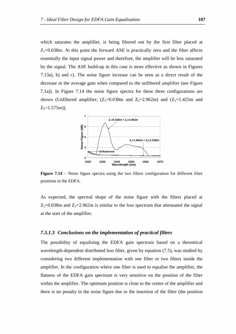
7-IdealFilterDesignforEDFAGainEqualisation 107
which saturates the amplifier, is being filtered out by the first filter placed at
Z1=0.038m.At thispoint theforwardASEispracticallyzeroand the filteraffects
essentiallytheinputsignalpowerandtherefore,theamplifierwillbelesssaturated
bythesignal.TheASEbuild-upinthiscaseismoreeffectiveasshowninFigures
7.13a), b) and c). The noise figure increase can be seen as a direct result of the
decreaseintheaveragegainwhencomparedtotheunfilteredamplifier(seeFigure
7.1a)). In Figure 7.14 the noise figure spectra for these three configurations are
shown (Unfiltered amplifier; (Z1=0.038m and Z2=2.962m) and (Z1=1.425m and
Z2=1.575m)).
3
4
5
6
7
1520 1530 1540 1550 1560 1570Wavelength(nm)
Noi
seF
igur
e(d
B)
Z1=0.038m+Z2=2.962m
Z1=1.462m+Z2=1.538m
Unflattened
Figure 7.14 – Noise figure spectra using the two filters configuration for different filter
positionsintheEDFA.
As expected, the spectral shape of the noise figure with the filters placed at
Z1=0.038mandZ2=2.962missimilartothelossspectrumthatattenuatedthesignal
atthestartoftheamplifier.
7.3.1.3 Conclusionsontheimplementationofpracticalfilters
The possibility of equalising the EDFA gain spectrum based on a theoretical
wavelength-dependentdistributedlossfilter,givenbyequation(7.5),wasstudiedby
considering two different implementation with one filter or two filters inside the
amplifier.Intheconfigurationwhereonefilterisusedtoequalisetheamplifier,the
flatness of the EDFA gain spectrum is very sensitive on the position of the filter
withintheamplifier.Theoptimumpositionisclosetothecentreoftheamplifierand
thereisnopenaltyinthenoisefigureduetotheinsertionofthefilter(theposition
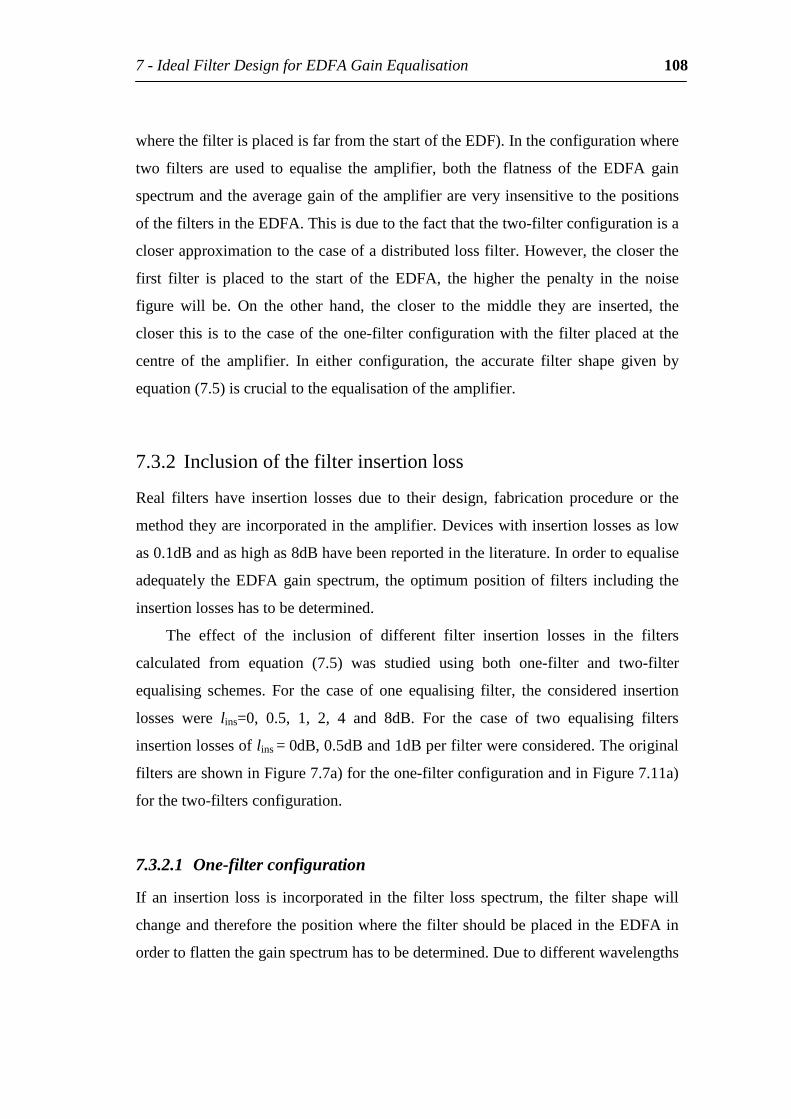
7-IdealFilterDesignforEDFAGainEqualisation 108
wherethefilterisplacedisfarfromthestartoftheEDF).Intheconfigurationwhere
two filters are used to equalise the amplifier, both the flatness of the EDFA gain
spectrumandtheaveragegainoftheamplifierareveryinsensitivetothepositions
ofthefiltersintheEDFA.Thisisduetothefactthatthetwo-filterconfigurationisa
closerapproximationtothecaseofadistributedlossfilter.However,thecloserthe
first filter is placed to the start of the EDFA, the higher the penalty in the noise
figure will be. On the other hand, the closer to the middle they are inserted, the
closer this is to thecaseof theone-filterconfigurationwiththefilterplacedat the
centre of the amplifier. In either configuration, the accurate filter shape given by
equation(7.5)iscrucialtotheequalisationoftheamplifier.
7.3.2 Inclusionofthefilterinsertionloss
Real filters have insertion losses due to their design, fabrication procedure or the
methodtheyareincorporatedintheamplifier.Deviceswithinsertionlossesaslow
as0.1dBandashighas8dBhavebeenreportedintheliterature.Inordertoequalise
adequately theEDFAgain spectrum, theoptimumpositionof filters including the
insertionlosseshastobedetermined.
The effect of the inclusion of different filter insertion losses in the filters
calculated from equation (7.5) was studied using both one-filter and two-filter
equalising schemes. For the case of one equalising filter, the considered insertion
losses were lins=0, 0.5, 1, 2, 4 and 8dB. For the case of two equalising filters
insertionlossesoflins=0dB,0.5dBand1dBperfilterwereconsidered.Theoriginal
filtersareshowninFigure7.7a)fortheone-filterconfigurationandinFigure7.11a)
forthetwo-filtersconfiguration.
7.3.2.1 One-filterconfiguration
If an insertion loss is incorporated in the filter loss spectrum, the filter shapewill
changeandthereforethepositionwherethefiltershouldbeplacedintheEDFAin
ordertoflattenthegainspectrumhastobedetermined.Duetodifferentwavelengths
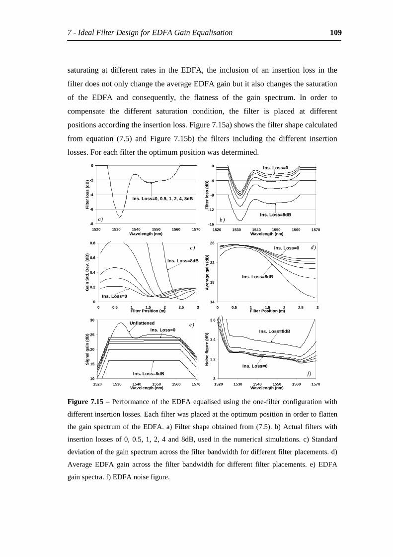
7-IdealFilterDesignforEDFAGainEqualisation 109
saturating at different rates in the EDFA, the inclusion of an insertion loss in the
filterdoesnotonlychangetheaverageEDFAgainbutitalsochangesthesaturation
of the EDFA and consequently, the flatness of the gain spectrum. In order to
compensate the different saturation condition, the filter is placed at different
positionsaccordingtheinsertionloss.Figure7.15a)showsthefiltershapecalculated
from equation (7.5) and Figure 7.15b) the filters including the different insertion
losses.Foreachfiltertheoptimumpositionwasdetermined.
-8
-6
-4
-2
0
1520 1530 1540 1550 1560 1570Wavelength(nm)
Filte
rlo
ss(d
B)
a)
Ins.Loss=0,0.5,1,2,4,8dB
-16
-12
-8
-4
0
1520 1530 1540 1550 1560 1570Wavelength(nm)
Filte
rlo
ss(d
B)
b)Ins.Loss=8dB
Ins.Loss=0
0
0.2
0.4
0.6
0.8
0 0.5 1 1.5 2 2.5 3FilterPosition(m)
Gai
nS
td.D
ev.(
dB)
c)
Ins.Loss=8dB
Ins.Loss=014
18
22
26
0 0.5 1 1.5 2 2.5 3FilterPosition(m)
Ave
rage
gai
n(d
B)
d)
Ins.Loss=8dB
Ins.Loss=0
10
15
20
25
30
1520 1530 1540 1550 1560 1570Wavelength(nm)
Sig
nalg
ain
(dB
)
e)
Ins.Loss=8dB
Ins.Loss=0Unflattened
3
3.2
3.4
3.6
1520 1530 1540 1550 1560 1570Wavelength(nm)
Noi
sefi
gure
(dB
)
f)
Ins.Loss=8dB
Ins.Loss=0
Figure7.15–Performanceof theEDFAequalisedusing theone-filterconfigurationwith
differentinsertionlosses.Eachfilterwasplacedattheoptimumpositioninordertoflatten
thegainspectrumof theEDFA.a)Filtershapeobtainedfrom(7.5).b)Actual filterswith
insertion lossesof0,0.5,1,2,4and8dB,used in thenumerical simulations.c)Standard
deviationofthegainspectrumacrossthefilterbandwidthfordifferentfilterplacements.d)
Average EDFA gain across the filter bandwidth for different filter placements. e) EDFA
gainspectra.f)EDFAnoisefigure.
7-IdealFilterDesignforEDFAGainEqualisation 110
For each filter the average and standard deviation of the equalised gain
spectrum for different filter positions was calculated. The results of these
simulationsareshowninFigures7.15d)and7.15c)respectively.Thefilterposition
thatgivestheloweststandarddeviationcorrespondstotheoptimumpositionofthe
filter.Fromtheseresultsitmaybeobservedthatthechangeintheoptimumposition
of the filter due to the insertion loss gives a penalty in the average gain of the
amplifier. However, equalisation of the EDFA gain spectrum is still achieved by
changing the position of the filters. The higher the insertion loss of the filter, the
closertotheendoftheEDFistheoptimumpositionandtheloweristheamplifier
averagegainacrossthefilterbandwidth.Thepenaltyintheaveragegainforfilters
placedattheoptimumpositioncorrespondsroughlytothefilterinsertionloss.Fora
filter with no insertion loss the optimum position is around Z1=1.575m and the
averagegain isclose to24dBandfora filterwith8dBinsertion loss theoptimum
positionisaroundZ1=2.5mandtheaveragegainis16dB.Figure7.15e)showsthe
EDFA gain spectrum for the filters with different insertion losses placed at the
optimumpositions.
The almost linear relation between the amplifier gain reduction and the filter
insertionlosscanbeunderstoodbyobservingthebehaviourofthepumppowerand
populationinversionalongtheEDF.Thepopulationinversionduetotheplacement
of the filter doesnot change significantly and therefore, there is no significant re-
absorptionofthepumpandnosignificantbuild-upoftheASEandsignalafterthe
filter.Figures7.16a)and7.16b)showrespectively,thepumppowerandpopulation
inversionalongtheEDFlengthforfilterswithdifferentinsertionlosses.
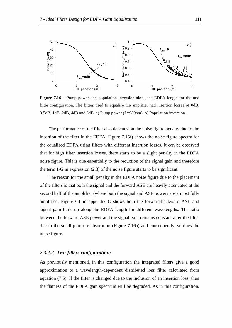
7-IdealFilterDesignforEDFAGainEqualisation 111
0
10
20
30
40
50
0 1 2 3EDFposition(m)
Pow
er(m
W)
a)
l Ins =0
l Ins =8dB0.4
0.5
0.6
0.7
0.8
0.9
1
0 1 2 3EDFposition(m)
Inve
rsio
nn
2/n
t(a.
u.) b)
l Ins =0
l Ins =8dB
84
0.51
0
2
Figure 7.16 – Pump power and population inversion along the EDFA length for the one
filter configuration.The filtersused to equalise the amplifierhad insertion lossesof0dB,
0.5dB,1dB,2dB,4dBand8dB.a)Pumppower(λ=980nm).b)Populationinversion.
Theperformanceofthefilteralsodependsonthenoisefigurepenaltyduetothe
insertionofthefilterintheEDFA.Figure7.15f)showsthenoisefigurespectrafor
theequalisedEDFAusingfilterswithdifferentinsertionlosses.Itcanbeobserved
that forhigh filter insertion losses, there starts tobea slightpenalty in theEDFA
noisefigure.Thisisdueessentiallytothereductionofthesignalgainandtherefore
theterm1/Ginexpression(2.8)ofthenoisefigurestartstobesignificant.
ThereasonforthesmallpenaltyintheEDFAnoisefigureduetotheplacement
ofthefiltersisthatboththesignalandtheforwardASEareheavilyattenuatedatthe
secondhalfoftheamplifier(whereboththesignalandASEpowersarealmostfully
amplified. Figure C1 in appendix C shows both the forward-backward ASE and
signal gain build-up along the EDFA length for different wavelengths. The ratio
betweentheforwardASEpowerandthesignalgainremainsconstantafterthefilter
due to the small pump re-absorption (Figure7.16a) andconsequently, sodoes the
noisefigure.
7.3.2.2 Two-filtersconfiguration:
As previously mentioned, in this configuration the integrated filters give a good
approximation to a wavelength-dependent distributed loss filter calculated from
equation(7.5).Ifthefilterischangedduetotheinclusionofaninsertionloss,then
theflatnessoftheEDFAgainspectrumwillbedegraded.Asinthisconfiguration,
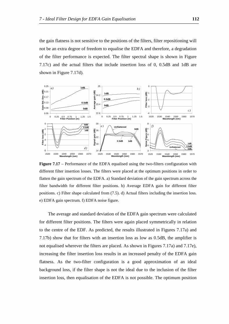
7-IdealFilterDesignforEDFAGainEqualisation 112
thegainflatnessisnotsensitivetothepositionsofthefilters,filterrepositioningwill
notbeanextradegreeoffreedomtoequalisetheEDFAandtherefore,adegradation
of the filter performance is expected. The filter spectral shape is shown in Figure
7.17c) and the actual filters that include insertion loss of 0, 0.5dB and 1dB are
showninFigure7.17d).
0.05
0.09
0.13
0.17
0.21
0.25
0 0.25 0.5 0.75 1 1.25 1.5FilterPosition(m)
Gai
nS
td.D
ev.(
dB)
a) 1dB
0.5dB
0dB
22.6
23.4
24.2
25
0 0.25 0.5 0.75 1 1.25 1.5FilterPosition(m)
Ave
rag
eg
ain
(dB
) b)1dB
0.5dB
0dB
-4
-3
-2
-1
0
1520 1530 1540 1550 1560 1570Wavelength(nm)
Filt
erlo
ss(
dB)
c)
-5
-4
-3
-2
-1
0
1520 1530 1540 1550 1560 1570Wavelength(nm)
Filt
erlo
ss(d
B)
d)
1dB0.5dB0dB
14
18
22
26
30
1520 1530 1540 1550 1560 1570Wavelength(nm)
Sig
nal
gai
n(
dB)
e)
1dB0.5dB
0dBUnflattened
3
4
5
6
7
8
1520 1530 1540 1550 1560 1570Wavelength(nm)
Noi
seF
igu
re(d
B)
f)
1dB0.5dB
0dBUnflattened
Figure7.17–PerformanceoftheEDFAequalisedusingthetwo-filtersconfigurationwith
differentfilterinsertionlosses.Thefilterswereplacedattheoptimumpositionsinorderto
flattenthegainspectrumoftheEDFA.a)Standarddeviationofthegainspectrumacrossthe
filter bandwidth for different filter positions. b) Average EDFA gain for different filter
positions.c)Filtershapecalculatedfrom(7.5).d)Actualfiltersincludingtheinsertionloss.
e)EDFAgainspectrum.f)EDFAnoisefigure.
TheaverageandstandarddeviationoftheEDFAgainspectrumwerecalculated
fordifferentfilterpositions.Thefilterswereagainplacedsymmetricallyinrelation
tothecentreof theEDF.Aspredicted, theresults illustratedinFigures7.17a)and
7.17b)showthatforfilterswithaninsertionlossas lowas0.5dB,theamplifier is
notequalisedwhereverthefiltersareplaced.AsshowninFigures7.17a)and7.17e),
increasingthefilterinsertionlossresultsinanincreasedpenaltyoftheEDFAgain
flatness. As the two-filter configuration is a good approximation of an ideal
backgroundloss,ifthefiltershapeisnottheidealduetotheinclusionofthefilter
insertionloss,thenequalisationoftheEDFAisnotpossible.Theoptimumposition
7-IdealFilterDesignforEDFAGainEqualisation 113
of the filters for all the considered insertion losses is Z1=0.038m and Z2=2.962m.
However,aspreviouslymentioned,theinsertionofthefirstfilternearthestartofthe
amplifier causes a high penalty in the amplifier noise figure. The two-filter
configuration does not have the flexibility to accommodate changes in the filter
shape resulting in deterioration of both the gain spectrum flatness and the noise
figure.Figures7.17e)and7.17f)showrespectively,thepenaltyintheamplifiergain
flatnessandnoisefigure.
7.3.2.3 Conclusionsontheinclusionofthefilterinsertionloss
Boththesuggestedconfigurations(one-filterandtwo-filter)offlatteningtheEDFA
gain spectrum using real filters with different insertion losses were analysed. The
two-filterconfiguration is shown tobedisadvantageouscompared to theone-filter
configuration when the filter insertion loss in considered. This is due to the
approximationofthetwo-filtersconfigurationtoadistributedlossandtherefore,itis
veryinsensitivetothepositionofthefiltersintheEDFAandresultsinpenaltiesin
boththeEDFAnoisefigureandthegainflatness(Figure7.17).
Using the one-filter configuration, the optimum position of the filter in the
EDFAchangesaccordingtotheinsertionlossofthefilter.Thehighertheinsertion
loss, the closer to the endof theEDFA is theoptimumposition (Figure7.15).At
these optimum positions the gain flatness is achieved but at the cost of a lower
average gain, due to the placement of the filter nearer to the end of the EDFA
(Figure7.15e). In this configuration theEDFA canbe correctly equalised and the
noise figure penalty is very small even for filters with insertion losses as high as
8dB.
7.3.3 Filterdesignscompensatingthedeviceowninsertionloss
Sofar,ithasbeenshownthathighperformancegain-flatteningopticalfilterscanbe
obtained, by converting an ideal wavelength-dependent distributed loss (equation
7-IdealFilterDesignforEDFAGainEqualisation 114
(7.5)), intoa lumplossplacedinasingleposition(one-filterconfiguration)or two
symmetricpositions(two-filterconfiguration)alongtheamplifierlength.
Inthissection,thepossibilityofincorporatingthedeviceowninsertionlossinto
thefiltershape,andcompensatingfor it, is investigated.This isaccomplishedina
manneropposite to theone followed in theprevious section.For thispurpose, the
localisedwavelength-independentdeviceinsertionlossisspreaduniformlyalongthe
amplifier length. In this respect, the device insertion loss can be considered as
additionalbackgroundloss,lBG,andequation(7.5)canbenowusedtoprovidethe
correctedgain-flatteningfilterspectrum.Intheone-filterconfigurationtheinsertion
losses of the filters were 0, 0.5, 1, 2, 4 and 8, all in dB units. For the two-filter
configurationeachfilterhadaninsertionlossof0dB,0.5dBand1dB.
7.3.3.1 One-filterconfiguration
ThetreatmentofthefilterinsertionlossasanequivalentEDFbackgroundlosswill
result in different filter shapes in order to equalise the gain spectrum. The
corrections in the filter loss spectrumdue to the inclusionof the fibrebackground
lossareshowninFigure7.3c).Thecorrectedfiltershapesforeachinsertionlossare
illustrated in Figure 7.18a) and the actual filters, including the insertion loss, are
showninFigure7.18b).
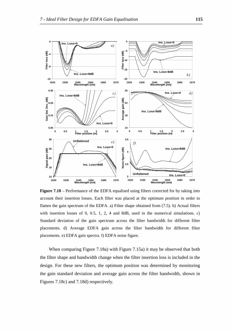
7-IdealFilterDesignforEDFAGainEqualisation 115
-12
-8
-4
0
1520 1530 1540 1550 1560 1570Wavelength(nm)
Filte
rlo
ss(d
B)
a)
Ins.Loss=8dB
Ins.Loss=0
-20
-15
-10
-5
0
1520 1530 1540 1550 1560 1570Wavelength(nm)
Filte
rlo
ss(d
B)
b)Ins.Loss=8dB
Ins.Loss=0
0.05
0.15
0.25
0.35
0 0.5 1 1.5 2 2.5 3Filterposition(m)
Gai
nS
td.D
ev.(
dB)
c)
Ins.Loss=0
Ins.Loss=8dB
14
18
22
26
0 0.5 1 1.5 2 2.5 3Filterposition(m)
Ave
rage
gai
n(d
B)
d)
Ins.Loss=8dB
Ins.Loss=0
14
18
22
26
30
1520 1530 1540 1550 1560 1570Wavelength(nm)
Sig
nalg
ain
(dB
)
e)Unflattened
Ins.Loss=0
Ins.Loss=8dB
3
3.5
4
4.5
1520 1530 1540 1550 1560 1570Wavelength(nm)
Noi
sefi
gure
(dB
)
f)
Unflattened
Ins.Loss=8dB
Ins.Loss=0
Figure7.18–PerformanceoftheEDFAequalisedusingfilterscorrectedforbytakinginto
account their insertion losses. Each filter was placed at the optimum position in order to
flattenthegainspectrumoftheEDFA.a)Filtershapeobtainedfrom(7.5).b)Actualfilters
with insertion losses of 0, 0.5, 1, 2, 4 and 8dB, used in the numerical simulations. c)
Standard deviation of the gain spectrum across the filter bandwidth for different filter
placements. d) Average EDFA gain across the filter bandwidth for different filter
placements.e)EDFAgainspectra.f)EDFAnoisefigure.
WhencomparingFigure7.18a)withFigure7.15a)itmaybeobservedthatboth
thefiltershapeandbandwidthchangewhenthefilterinsertionlossisincludedinthe
design.For thesenewfilters, theoptimumpositionwasdeterminedbymonitoring
thegainstandarddeviationandaveragegainacross thefilterbandwidth,shownin
Figures7.18c)and7.18d)respectively.
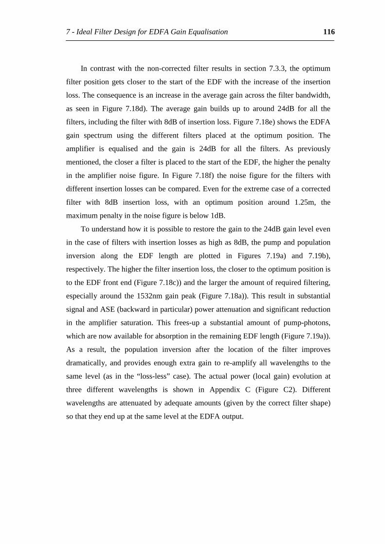
7-IdealFilterDesignforEDFAGainEqualisation 116
In contrast with the non-corrected filter results in section 7.3.3, the optimum
filterpositiongetscloser to the startof theEDFwith the increaseof the insertion
loss.Theconsequenceisanincreaseintheaveragegainacrossthefilterbandwidth,
as seen in Figure 7.18d). The average gain builds up to around 24dB for all the
filters,includingthefilterwith8dBofinsertionloss.Figure7.18e)showstheEDFA
gain spectrum using the different filters placed at the optimum position. The
amplifier is equalised and the gain is 24dB for all the filters. As previously
mentioned,thecloserafilterisplacedtothestartoftheEDF,thehigherthepenalty
in the amplifier noise figure. In Figure 7.18f) the noise figure for the filters with
differentinsertionlossescanbecompared.Evenfortheextremecaseofacorrected
filter with 8dB insertion loss, with an optimum position around 1.25m, the
maximumpenaltyinthenoisefigureisbelow1dB.
Tounderstandhowitispossibletorestorethegaintothe24dBgainleveleven
inthecaseoffilterswithinsertionlossesashighas8dB,thepumpandpopulation
inversion along the EDF length are plotted in Figures 7.19a) and 7.19b),
respectively.Thehigherthefilterinsertionloss,theclosertotheoptimumpositionis
totheEDFfrontend(Figure7.18c))andthelargertheamountofrequiredfiltering,
especially around the1532nmgainpeak (Figure7.18a)).This result in substantial
signalandASE(backwardinparticular)powerattenuationandsignificantreduction
in the amplifier saturation. This frees-up a substantial amount of pump-photons,
whicharenowavailableforabsorptionintheremainingEDFlength(Figure7.19a)).
As a result, the population inversion after the location of the filter improves
dramatically, and provides enough extra gain to re-amplify all wavelengths to the
same level (as in the “loss-less” case). The actual power (local gain) evolution at
three different wavelengths is shown in Appendix C (Figure C2). Different
wavelengthsareattenuatedbyadequateamounts(givenbythecorrectfiltershape)
sothattheyendupatthesamelevelattheEDFAoutput.
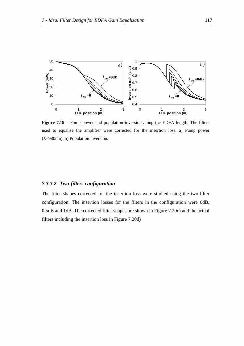
7-IdealFilterDesignforEDFAGainEqualisation 117
0
10
20
30
40
50
0 1 2 3EDFposition(m)
Pow
er(m
W)
a)
l Ins =0
l Ins =8dB
0.4
0.5
0.6
0.7
0.8
0.9
1
0 1 2 3EDFposition(m)
Inve
rsio
nn 2
/nt(
a.u.
) b)
l Ins =0
l Ins =8dB
Figure 7.19 – Pump power and population inversion along the EDFA length. The filters
used to equalise the amplifier were corrected for the insertion loss. a) Pump power
(λ=980nm).b)Populationinversion.
7.3.3.2 Two-filtersconfiguration
The filter shapes corrected for the insertion loss were studied using the two-filter
configuration. The insertion losses for the filters in the configuration were 0dB,
0.5dBand1dB.ThecorrectedfiltershapesareshowninFigure7.20c)andtheactual
filtersincludingtheinsertionlossinFigure7.20d)
7-IdealFilterDesignforEDFAGainEqualisation 118
0.04
0.08
0.12
0.16
0 0.25 0.5 0.75 1 1.25 1.5FilterPosition(m)
Gai
nS
td.D
ev.(
dB
) a)1dB
0.5dB
0dB
22
23
24
25
0 0.25 0.5 0.75 1 1.25 1.5FilterPosition(m)
Ave
rag
eG
ain
(dB
)
b)1dB
0.5dB
0dB
-5
-4
-3
-2
-1
0
1520 1530 1540 1550 1560 1570Wavelength(nm)
Filt
erlo
ss(
dB
)
c)1dB
0dB0dB
1dB
-6
-4
-2
0
1520 1530 1540 1550 1560 1570Wavelength(nm)
Filt
erlo
ss(
dB
)
d)
1dB0.5dB0dB
14
18
22
26
30
1520 1530 1540 1550 1560 1570Wavelength(nm)
Sig
nal
gai
n(
dB
)
e)
1dB0.5dB
0dBUnflattened
3
3.2
3.4
3.6
3.8
4
1520 1530 1540 1550 1560 1570Wavelength(nm)
No
ise
Fig
ure
(dB
)
f)
1dB
0.5dB
0dB
Unflattened
Figure 7.20 – EDFA performance for the amplifier equalised using the two-filters
configurationwithdifferentinsertionlosses.Thefilterdesignwascorrectedfortheinsertion
lossandeachfilterwasplacedattheoptimumpositioninordertoflattenthegainspectrum
of the EDFA. a) Standard deviation of the gain spectrum across the filter bandwidth. b)
Average EDFA gain across the filter bandwidth. c) Filter shape calculated from (7.5). d)
Filterincludingtheinsertionloss.e)EDFAgainspectra.f)EDFAnoisefigure.
Thestandarddeviationofthegainspectrumandtheaveragegainfordifferent
filterpositionswerecalculatedfor thecorrectedfilterprofiles.Theresults indicate
that forall the insertionlosses, thecorrectedfilters,shouldbeplacedatZ1=1.35m
and Z2=1.65m in order to optimise the flatness of the gain spectrum, as seen in
Figure7.20a).Thesepositionsalsocorrespondtomaximaoftheaveragegainacross
eachfilterbandwidth(Figure7.20b).AgoodEDFAequalisationwasnotachieved
withaninsertionlossof1dBperfilter.Thismeansthattheassumptionthatthefilter
insertionlosscanbetreatedasafibrebackgroundlossisnottotallyaccurateandfor
high insertion losses EDFA equalisation is not perfectly achieved. Comparing the
placementofthecorrectedfilterdesignsshowninFigure7.20a),withtheplacement
oftheuncorrectedfilterdesignsshowninFigure7.17a),itisobservedthattheyare
both quite insensitive to the position of the filters. However the corrected filters
shouldbeplacedcloser to thecentreof theEDF toachieveEDFAgain flattening
whiletheun-correctedfiltersshouldbeplacedattheendsoftheEDF.Thepenalty
intheaveragegainacrossthefilterbandwidthissimilarinbothfiltershapesbutthe
7-IdealFilterDesignforEDFAGainEqualisation 119
noisefigurefortheuncorrectedfiltersismuchhigherduetotheplacementofoneof
thefiltersclosetothestartof theamplifier. Inthecaseof thecorrectedfilters, the
noisefigure(Figure7.20f)islowduetothefiltersbeingplacedneartothemiddleof
theEDF.Itisalsoobservedthattheachievedgainflatteningisalsoimprovedwhen
usingthecorrectedfiltershapes(Figure7.20e).
7.3.3.3 Conclusions on the correction of the filter to compensate for the
deviceinsertionloss
Boththesuggestedconfigurations(one-filterandtwo-filter)offlatteningtheEDFA
gain spectrum using real filters with loss spectra corrected for different insertion
losseswereanalysed.The two-filter configuration is shown tobedisadvantageous
comparedtotheone-filterconfigurationwhenthefilterinsertionlossinconsidered.
However, using the corrected filter shapes there is a slight improvement of the
EDFAgainspectrumflatnessandnoisefigureforthetwo-filterconfiguration.This
configurationcouldbeused in realamplifiersusing filterswithvery lowinsertion
losses. The two-filter configuration also halves the requirements on maximum
filtering loss, which eases the implementation and manufacture of the different
filters.Twolongperiodgratingscouldbeusedoralternatively,onestaticfilterand
an AO tunable filter could be used in order to achieve dynamic equalisation. The
mainadvantageofusingthisconfigurationisthatthefilterpositioningisnotcritical
fortheperformanceoftheamplifierequalisation.
Usingtheone-filterconfiguration,theoptimumpositionofthecorrectedfilters
in the EDFA changes according to the insertion loss of the filter. The higher the
insertionloss,theclosertothestartoftheEDFAlaystheoptimumposition(Figure
7.18). This behaviour is opposite to the one shown by the positioning of the un-
corrected filters in theEDFA (Figure7.15).Using thecorrected filters, theEDFA
gainspectrumwasequalisedwithnopenaltyintheaveragegainevenwithinsertion
lossesupto8dB.Thepenaltyintheamplifiernoisefigureduetotheintroductionof
these filters was bellow 1dB. This configuration however, allows a better gain
7-IdealFilterDesignforEDFAGainEqualisation 120
equalisation.Ontheotherhand,theperformanceoftheequalisedamplifierdepends
on the exact positioning of the filters and, therefore, may prove more difficult to
implement.
7.3.4 EDFAEqualisationbyusingtheinverseofthegainspectrum
Itiscommonpracticetoplacetheequalisingfilterattheoutputoftheamplifier.The
EDFA gain flattening performance using the one-filter configuration (Figure 7.7)
andusingtheinversegainprofileastheequalisingfilterisshowninFigure7.21.In
order to correctly flatten the EDFA gain spectrum, the inverse shape of the gain
spectrumacrossadesiredbandwidthisused(Figure7.21a).Inordertocharacterise
theperformanceof theequalisationof theEDFAgainspectrumusingfiltersbased
ontheinverseofthegainspectrum,theaverageandstandarddeviationofthegain
spectrum were calculated for different filter placements along the EDF. The filter
loss spectrum was obtained by selecting a bandwidth across the EDFA gain
spectrum(Figure7.21b).Filterinsertionlossesof0,0.5dB,1dB,2dB,4dBand8dB
wereconsideredinthenumericalsimulations(Figure7.21e).Itisexpectedthatthe
optimum positions where the filters should be placed are close to the end of the
EDFA and the standard deviation of the gain spectrum should increase when the
filtersareplacedclosertothestartoftheEDF.
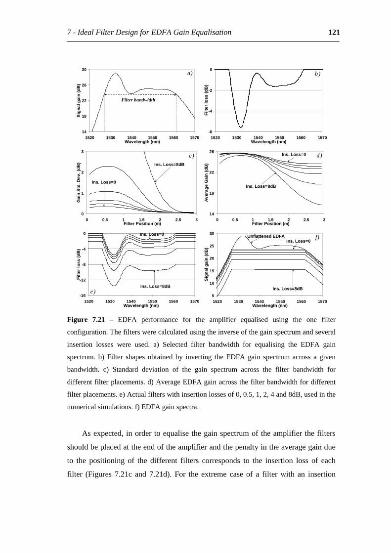
7-IdealFilterDesignforEDFAGainEqualisation 121
14
18
22
26
30
1520 1530 1540 1550 1560 1570Wavelength(nm)
Sig
nalg
ain
(dB
)a)
Filterbandwidth
-6
-4
-2
0
1520 1530 1540 1550 1560 1570Wavelength(nm)
Filte
rlo
ss(d
B)
b)
0
1
2
3
0 0.5 1 1.5 2 2.5 3FilterPosition(m)
Gai
nS
td.D
ev.(
dB)
c)Ins.Loss=8dB
Ins.Loss=0
14
18
22
26
0 0.5 1 1.5 2 2.5 3FilterPosition(m)
Ave
rage
Gai
n(d
B)
d)
Ins.Loss=8dB
Ins.Loss=0
-16
-12
-8
-4
0
1520 1530 1540 1550 1560 1570Wavelength(nm)
Filte
rlo
ss(d
B)
e)Ins.Loss=8dB
Ins.Loss=0
5
10
15
20
25
30
1520 1530 1540 1550 1560 1570Wavelength(nm)
Sig
nalg
ain
(dB
)
f)Ins.Loss=0
Ins.Loss=8dB
UnflattenedEDFA
Figure 7.21 – EDFA performance for the amplifier equalised using the one filter
configuration.Thefilterswerecalculatedusingtheinverseofthegainspectrumandseveral
insertion losses were used. a) Selected filter bandwidth for equalising the EDFA gain
spectrum. b) Filter shapes obtained by inverting the EDFA gain spectrum across a given
bandwidth. c) Standard deviation of the gain spectrum across the filter bandwidth for
differentfilterplacements.d)AverageEDFAgainacrossthefilterbandwidthfordifferent
filterplacements.e)Actualfilterswithinsertionlossesof0,0.5,1,2,4and8dB,usedinthe
numericalsimulations.f)EDFAgainspectra.
Asexpected, inorder toequalisethegainspectrumoftheamplifier thefilters
shouldbeplacedattheendoftheamplifierandthepenaltyintheaveragegaindue
to the positioning of the different filters corresponds to the insertion loss of each
filter (Figures 7.21c and 7.21d). For the extreme case of a filter with an insertion
7-IdealFilterDesignforEDFAGainEqualisation 122
lossof8dBthegaindecreasesfrom24dBtoapproximately16dB.Withtheincrease
of the filter insertion loss thegainof the amplifierdecreases. InFigure7.21f) the
gain spectra for the EDFA equalised with the different filters are illustrated.
However,duetothefilterbeingplacedattheendoftheEDF,thereisfurthersignal
andforwardASEbuild-upandthereforenobroadeningoftheEDFAgainspectrum
duetothedifferentsaturationconditionsaftertheinclusionofthefilter,asseenin
Figures 7.15e) and 7.18e). The noise figure remains unchanged due to the equal
attenuationof the signaland forwardASEspectrumby the filterat the endof the
amplifier.
Theresultsof theequalisationof theEDFAgainspectrumaresimilar inboth
thecasesoffiltersuncorrectedfortheinsertionloss,calculatedfromequation(7.5),
placedwithintheEDFAandthepresentcasewheretheinverseofthegainspectrum
is used to equalise the EDFA gain spectrum. In both cases the EDFA is well
equalised and the penalty in the amplifier gain due to the insertion of filters
correspondstotheirinsertionlosses.
Insummary,using this technique,goodgainflatnesscanbeachievedwithno
penalty in the amplifier noise figure. However, there is no increase in the filter
bandwidthduetore-amplificationwithdifferentsaturationconditionsasseenwhen
thefilterisplacedclosertothecentreoftheamplifier,seeFigures7.15e)and7.18e).
Thepenaltyintheaveragegainacrossthefilterbandwidthduetotheinsertionloss
ofthefiltercorrespondstothedeviceinsertionloss.
7.3.5 Conclusions
AsummaryoftheresultsofthesimulationssofarisshowninFigure7.22wherethe
EDFA noise figure at λ=1532nm, the gain standard deviation and average gain
acrossthefilterbandwidtharecomparedfortheone-filterconfigurationwhenusing
the three types of filters considered: Filters that were corrected for the insertion
losses, theuncorrectedonesandthefiltersbasedontheinverseof thegainprofile
placedattheoutputoftheEDFA.
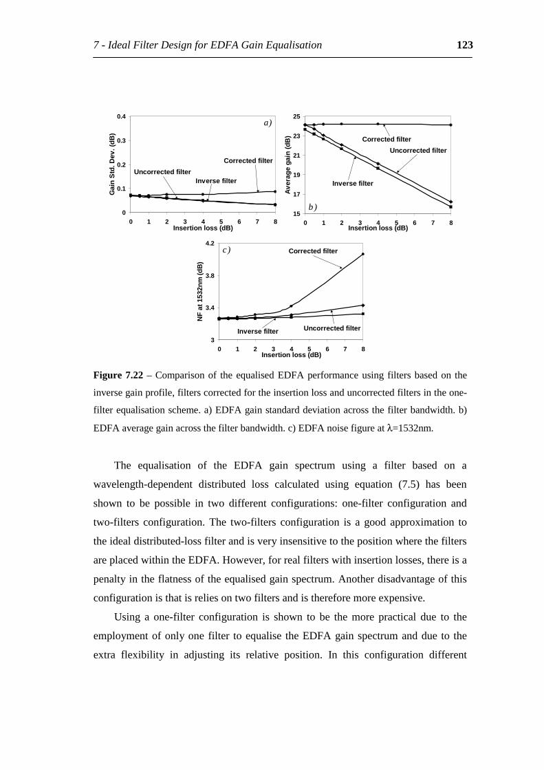
7-IdealFilterDesignforEDFAGainEqualisation 123
0
0.1
0.2
0.3
0.4
0 1 2 3 4 5 6 7 8Insertionloss(dB)
Gai
nS
td.D
ev.(
dB)
a)
Inversefilter
Correctedfilter
Uncorrectedfilter
15
17
19
21
23
25
0 1 2 3 4 5 6 7 8Insertionloss(dB)
Ave
rage
gai
n(d
B)
Inversefilter
Correctedfilter
b)
Uncorrectedfilter
3
3.4
3.8
4.2
0 1 2 3 4 5 6 7 8Insertionloss(dB)
NF
at1
532n
m(d
B)
c)
Inversefilter
Correctedfilter
Uncorrectedfilter
Figure7.22–Comparisonof theequalisedEDFAperformanceusing filtersbasedon the
inversegainprofile,filterscorrectedfortheinsertionlossanduncorrectedfiltersintheone-
filterequalisationscheme.a)EDFAgainstandarddeviationacrossthefilterbandwidth.b)
EDFAaveragegainacrossthefilterbandwidth.c)EDFAnoisefigureatλ=1532nm.
The equalisation of the EDFA gain spectrum using a filter based on a
wavelength-dependent distributed loss calculated using equation (7.5) has been
shown to be possible in two different configurations: one-filter configuration and
two-filters configuration. The two-filters configuration is a good approximation to
theidealdistributed-lossfilterandisveryinsensitivetothepositionwherethefilters
areplacedwithintheEDFA.However,forrealfilterswithinsertionlosses,thereisa
penaltyintheflatnessoftheequalisedgainspectrum.Anotherdisadvantageofthis
configurationisthatisreliesontwofiltersandisthereforemoreexpensive.
Using a one-filter configuration is shown to be the more practical due to the
employmentofonlyonefilter toequalise theEDFAgainspectrumanddue to the
extra flexibility in adjusting its relative position. In this configuration different
7-IdealFilterDesignforEDFAGainEqualisation 124
equalisationschemesfortheEDFAgainspectrumwerecomparedinFigure7.22:1-
Equalisationusingfilterscalculatedfromequation(7.5)thatwerecorrectedfortheir
insertionloss;2-Equalisationusingfilterscalculatedfromequation(7.3)thatwere
not corrected for their insertion losses; 3- equalisation using filters based on the
inverseprofileofthegainspectrumthatwereplacedattheoutputoftheEDFA.The
thirdequalisationschemeis themostcommonlyadopted inequalisingEDFAgain
spectra.Inalloftheschemes,gainflatnessisachievedattheoptimumpositionsfor
allfilters.Boththeuncorrectedfiltersplacedattheoptimumpositionsandthefilters
basedontheinverseofthegainspectrumhavesimilarperformanceintermsofgain
standarddeviation,averagegainandnoise figure.However,whenusing thefilters
correctedfortheinsertionlossitisobservedthatthereisasignificantimprovement
in theEDFA gainwith small penalty in the gain spectrumstandarddeviation and
noisefigure(seeFigures7.22a),b)andc),respectively).Inthisconfiguration,there
isatotalrecoveryintheamplifiergainandlowpenaltyinthenoisefigureevenfor
filters with insertion losses as high as 8dB. The design and positioning of these
novel filters improves the overall performance of equalised EDFAs. Another
advantageofbothschemes1and2,inrelationtoscheme3,istheslightlyincreased
useful bandwidth obtained, as shown in Figures 7.15e) and 7.18e), respectively,
comparedtoscheme3,showninFigure7.21f).
7.4 Gain flattening filters compensating for the insertion
lossesofotherdevices
In the following section, thiswork is extendedeven further to thedesignofgain-
flatteningfiltersthatcancompensateforinsertionlossesofdifferentdevicesplaced
alongtheEDFAaswellastheirowninsertionloss.Firstly,inordertodemonstrate
theprinciple, thecaseofa lumplossof2dBplacedatagivenpositionwithin the
EDFA is considered. This loss could correspond to the insertion loss of a tap or
anotherfilteringdeviceor lossesduetosplicing.Thesefiltercalculationscouldbe
7-IdealFilterDesignforEDFAGainEqualisation 125
applied generally, to a number of distributed sources of loss within the EDFA.
Secondly, the inclusionofan isolator in theEDFAisconsidered.The isolator isa
special component commonlyused in amplifiers inorder to reduce the amountof
lighttravellinginthereversedirectionandarrivingattheamplifierinput.Thislight
is due mainly to backward propagating amplified spontaneous emission. The
placementofanisolatorintheEDFAisalsoknowntoimprovetheamplifiernoise
figureandsignalgainwhenplacedat theoptimumposition[108].Toequalise the
EDFA+isolatorstructure,theoptimumpositionwheretheisolatorshouldbeplaced
was determined and the equalising filter was designed in order to compensate for
bothitsowninsertionlossaswellastheinsertionlossoftheisolator.
7.4.1 Equalisation of the EDFA with a lump loss positioned at
Z=2m
ApossibleconfigurationforanEDFAcouldincludeatapdeviceformonitoringthe
performanceoftheEDFAatagivenposition.Theinsertionlossofthesedevicesis
in general low (worst case of around 2dB) but will affect, nevertheless, the
saturationandgainoftheamplifier.TheequalisationoftheEDFAwiththelumped
losscanbeachievedbyinvertingthegainspectrumacrossadesiredbandwidthor,
as shown previously in section 7.3, by determining a filter shape from the ideal
background loss and placing it at the correct position in the EDFA. Figure 7.23
shows the EDFA configuration for a device with a certain insertion loss and an
equalising filter. The position where the tap device is placed is Zloss and the
equalisingfilterisplacedatZ1.
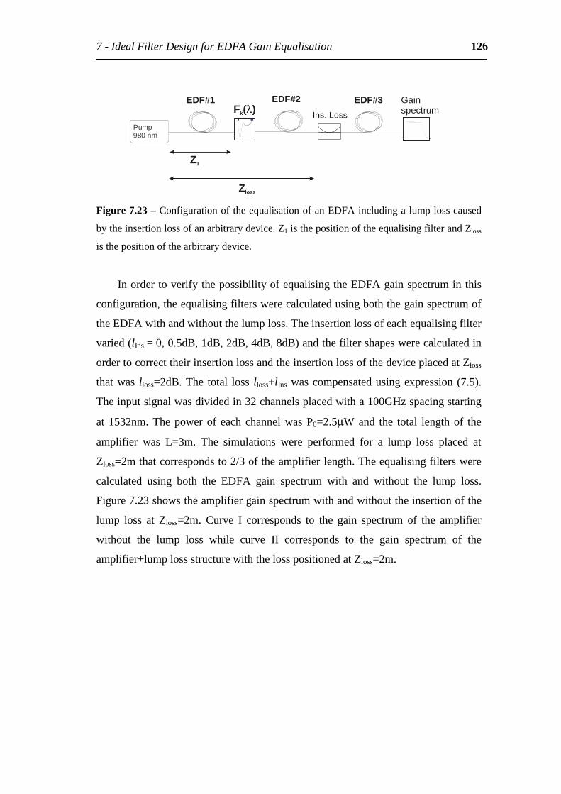
7-IdealFilterDesignforEDFAGainEqualisation 126
Pump980nm
Z1
Zloss
EDF#1 EDF#2 EDF#3
Ins.LossF ( )k λGainspectrum
Figure7.23–ConfigurationoftheequalisationofanEDFAincludingalumplosscaused
bytheinsertionlossofanarbitrarydevice.Z1isthepositionoftheequalisingfilterandZloss
isthepositionofthearbitrarydevice.
InordertoverifythepossibilityofequalisingtheEDFAgainspectruminthis
configuration,theequalisingfilterswerecalculatedusingboththegainspectrumof
theEDFAwithandwithoutthelumploss.Theinsertionlossofeachequalisingfilter
varied(lIns=0,0.5dB,1dB,2dB,4dB,8dB)andthefiltershapeswerecalculatedin
ordertocorrecttheirinsertionlossandtheinsertionlossofthedeviceplacedatZloss
thatwas lloss=2dB.The total loss lloss+lInswascompensatedusingexpression (7.5).
Theinputsignalwasdividedin32channelsplacedwitha100GHzspacingstarting
at 1532nm.Thepower of each channelwasP0=2.5µWand the total lengthof the
amplifier was L=3m. The simulations were performed for a lump loss placed at
Zloss=2mthatcorrespondsto2/3oftheamplifierlength.Theequalisingfilterswere
calculated using both the EDFA gain spectrum with and without the lump loss.
Figure7.23showstheamplifiergainspectrumwithandwithouttheinsertionofthe
lump loss at Zloss=2m. Curve I corresponds to the gain spectrum of the amplifier
without the lump loss while curve II corresponds to the gain spectrum of the
amplifier+lumplossstructurewiththelosspositionedatZloss=2m.
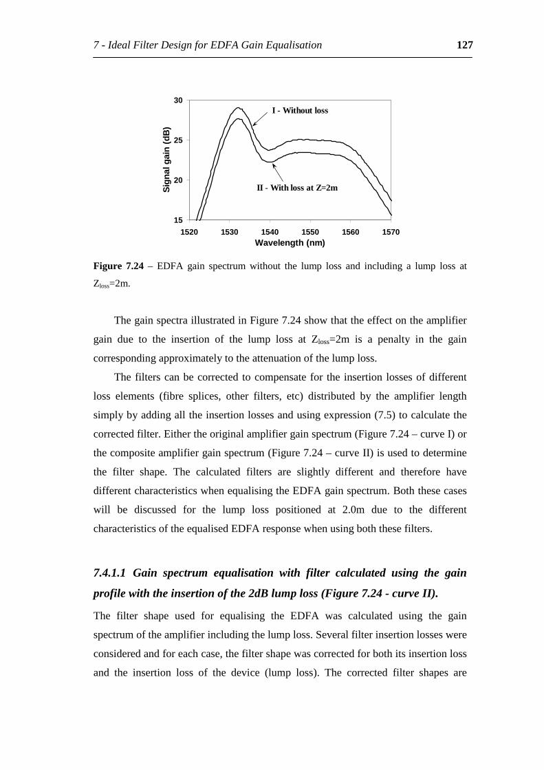
7-IdealFilterDesignforEDFAGainEqualisation 127
15
20
25
30
1520 1530 1540 1550 1560 1570Wavelength(nm)
Sig
nalg
ain
(dB
)
I-Withoutloss
II-WithlossatZ=2m
Figure 7.24 – EDFA gain spectrum without the lump loss and including a lump loss at
Zloss=2m.
ThegainspectraillustratedinFigure7.24showthattheeffectontheamplifier
gain due to the insertion of the lump loss at Zloss=2m is a penalty in the gain
correspondingapproximatelytotheattenuationofthelumploss.
Thefilterscanbecorrected tocompensate for the insertion lossesofdifferent
loss elements (fibre splices, other filters, etc) distributed by the amplifier length
simplybyaddingalltheinsertionlossesandusingexpression(7.5)tocalculatethe
correctedfilter.Eithertheoriginalamplifiergainspectrum(Figure7.24–curveI)or
thecompositeamplifiergainspectrum(Figure7.24–curveII)isusedtodetermine
the filter shape. The calculated filters are slightly different and therefore have
differentcharacteristicswhenequalisingtheEDFAgainspectrum.Boththesecases
will be discussed for the lump loss positioned at 2.0m due to the different
characteristicsoftheequalisedEDFAresponsewhenusingboththesefilters.
7.4.1.1 Gain spectrum equalisation with filter calculated using the gain
profilewiththeinsertionofthe2dBlumploss(Figure7.24-curveII).
The filter shape used for equalising the EDFA was calculated using the gain
spectrumoftheamplifierincludingthelumploss.Severalfilterinsertionlosseswere
consideredandforeachcase,thefiltershapewascorrectedforbothitsinsertionloss
and the insertion loss of the device (lump loss). The corrected filter shapes are
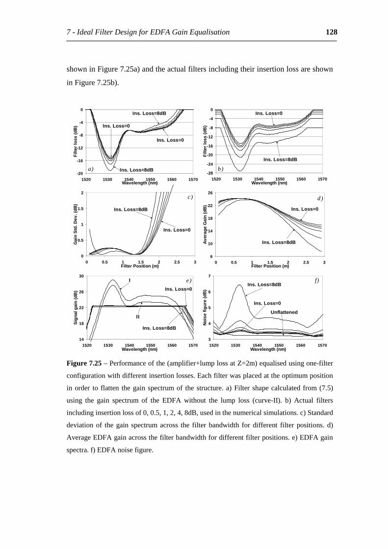
7-IdealFilterDesignforEDFAGainEqualisation 128
showninFigure7.25a)andtheactualfiltersincludingtheirinsertionlossareshown
inFigure7.25b).
-20
-16
-12
-8
-4
0
1520 1530 1540 1550 1560 1570Wavelength(nm)
Filte
rlo
ss(d
B)
a)
Ins.Loss=0
Ins.Loss=8dB
Ins.Loss=0
Ins.Loss=8dB
-28
-24
-20
-16
-12
-8
-4
0
1520 1530 1540 1550 1560 1570Wavelength(nm)
Filte
rlo
ss(d
B)
b)
Ins.Loss=0
Ins.Loss=8dB
0
0.5
1
1.5
2
0 0.5 1 1.5 2 2.5 3FilterPosition(m)
Gai
nS
td.D
ev.(
dB)
c)
Ins.Loss=0
Ins.Loss=8dB
6
10
14
18
22
26
0 0.5 1 1.5 2 2.5 3FilterPosition(m)
Ave
rage
Gai
n(d
B)
d)
Ins.Loss=0
Ins.Loss=8dB
14
18
22
26
30
1520 1530 1540 1550 1560 1570Wavelength(nm)
Sig
nalg
ain
(dB
)
e)I
Ins.Loss=0
Ins.Loss=8dB
II
3
4
5
6
7
1520 1530 1540 1550 1560 1570Wavelength(nm)
Noi
sefi
gure
(dB
)
f)
Unflattened
Ins.Loss=0
Ins.Loss=8dB
Figure7.25–Performanceofthe(amplifier+lumplossatZ=2m)equalisedusingone-filter
configurationwithdifferentinsertionlosses.Eachfilterwasplacedattheoptimumposition
inorder to flatten thegainspectrumof the structure.a)Filter shapecalculatedfrom(7.5)
using the gain spectrum of the EDFA without the lump loss (curve-II). b) Actual filters
includinginsertionlossof0,0.5,1,2,4,8dB,usedinthenumericalsimulations.c)Standard
deviationof thegain spectrumacross the filter bandwidth fordifferent filterpositions. d)
AverageEDFAgainacrossthefilterbandwidthfordifferentfilterpositions.e)EDFAgain
spectra.f)EDFAnoisefigure.
7-IdealFilterDesignforEDFAGainEqualisation 129
Byvarying thepositionof the filters along the amplifier length, theoptimum
positionswherethefiltersshouldbeplacedweredetermined.Theaveragegainand
standard deviation across the filter bandwidth were determined for different filter
positionsalongtheEDFA.Figures7.25d)and7.25c)showrespectively,theaverage
gainandstandarddeviationof theamplifierfor filterswithinsertionlossesof0to
8dBplacedalongtheamplifierlength.FromFigure7.25c)itmaybeobservedthat
theoptimumpositionsarearoundZ=1.3mor,atthestartoftheamplifier.Itisbest
toplace the filter away from the start of theEDF tominimise the amplifiernoise
figure penalty. Figures 7.25e) and 7.25f) show respectively the amplifier gain
spectrum and noise figure for filters placed at the optimum positions (around
Z=1.3m).
Equalisation of the EDFA gain spectrum was achieved for all the filters.
However, for filters with insertion losses over 4dB, a considerable penalty in the
noisefigureisobserved,duetotheplacementofthesefiltersclosertothestartofthe
amplifier. The insertion loss of each of the filters was compensated as shown in
Figure7.25e).Evenforfilterswithaninsertionlossof8dBthegainspectrumwas
equalised with full recovery of the average gain across the filter bandwidth. The
insertionlossofthelumplosswascompensatedbythefilterdesign.However,there
isapenaltyofroughly2dBcorrespondingtothelumplossthatisnotavoidedwhen
usingthecurrentfilters.
The way these filters achieve spectral equalisation of the amplifier gain is
shown in Figure C3 in appendix C where the signal gain, forward ASE and
backwardASEareplottedalongtheEDFlengthforthreedifferentwavelengths,λ1
=1532.3nm,λ2=1539.7nmandλ3=1550.9nm.Thereisaconstantinsertionlossof
2dBat Z=2mand the equalising filterswith insertion lossesof0, 0.5, 1, 2, 4 and
8dBareplacedat theoptimumpositions(aroundZ=1.3m). Inorder toobtaingain
equalisation across the whole filter bandwidth, the filter loss spectrum and the
positionwhere it isplacedhas tobe adjustedso thateachwavelength reaches the
endoftheamplifierwiththesamegainlevel.InFigureC3,itcanalsobeobserved
that even for filters with high insertion losses the gain can be recovered by the
correctdesignandpositioningofthefilters.
7-IdealFilterDesignforEDFAGainEqualisation 130
Thephysicalreasonforthesignalrecoveryandgainrestorationacrossthefilter
bandwidthisthesameasinthecasedescribedinsection7.3.3.1.Thesignalpower
andlocalgainevolutionforthreedifferentwavelengthsareshowninFiguresC3a),
b)andc),inAppendixC.Thepumppowerandpopulationinversionre-distribution
(due tochanges inEDFAsaturationcausedby thefiltering)along theEDFlength
areshowninFigureC4.
7.4.1.2 Gain spectrum equalisation with filter calculated using the gain
profilewiththeinsertionofthe2dBlumploss(Figure7.24-curveI).
In the following simulation the gain spectrum of the EDFA plus an insertion loss
placedatZloss=2misequalisedusingafiltercalculatedusingequation(7.5)andthe
amplifier gain spectrum without the lump loss (Curve I in Figure 7.24). Filter
insertion losses of 0, 0.5, 1, 2, 4 and 8dB were considered and for each case, the
filter loss spectrum was corrected for both its own insertion loss as well as the
insertionlossofthelosselementplacedatZloss=2m.Thecorrectedfiltershapesare
showninFigure7.26a)andtheactualFiltersincludingtheirinsertionlossareshown
inFigure7.26b).
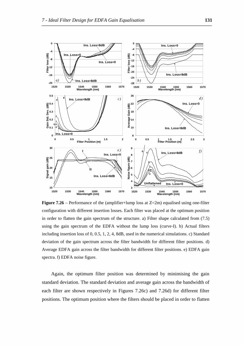
7-IdealFilterDesignforEDFAGainEqualisation 131
-20
-16
-12
-8
-4
0
1520 1530 1540 1550 1560 1570Wavelength(nm)
Filte
rlo
ss(d
B)
a)
Ins.Loss=0
Ins.Loss=8dB
Ins.Loss=0
Ins.Loss=8dB
-28
-24
-20
-16
-12
-8
-4
0
1520 1530 1540 1550 1560 1570Wavelength(nm)
Filte
rlo
ss(d
B)
b)
Ins.Loss=0
Ins.Loss=8dB
0
0.1
0.2
0.3
0.4
0.5
0 0.5 1 1.5 2FilterPosition(m)
Gai
nS
td.D
ev.(
dB)
c)
Ins.Loss=0
Ins.Loss=8dB84
2
1
00.5
6
10
14
18
22
26
0 0.5 1 1.5 2 2.5 3FilterPosition(m)
Ave
rage
Gai
n(d
B)
d)Ins.Loss=0
Ins.Loss=8dB
10
15
20
25
30
1520 1530 1540 1550 1560 1570Wavelength(nm)
Sig
nalg
ain
(dB
)
IIns.Loss=0
Ins.Loss=8dB
II
e)
3
4
5
6
7
8
9
1520 1530 1540 1550 1560 1570Wavelength(nm)
Noi
sefi
gure
(dB
)
f)
Unflattened Ins.Loss=0
Ins.Loss=8dB
0.5
0
1
2
48
Figure7.26–Performanceofthe(amplifier+lumplossatZ=2m)equalisedusingone-filter
configurationwithdifferentinsertionlosses.Eachfilterwasplacedattheoptimumposition
inorder to flatten thegainspectrumof the structure.a)Filtershapecalculatedfrom(7.5)
using the gain spectrum of the EDFA without the lump loss (curve-I). b) Actual filters
includinginsertionlossof0,0.5,1,2,4,8dB,usedinthenumericalsimulations.c)Standard
deviationof thegain spectrumacross the filter bandwidth fordifferent filter positions. d)
AverageEDFAgainacrossthefilterbandwidthfordifferentfilterpositions.e)EDFAgain
spectra.f)EDFAnoisefigure.
Again, the optimum filter position was determined by minimising the gain
standarddeviation.Thestandarddeviationandaveragegainacrossthebandwidthof
each filter are shown respectively in Figures 7.26c) and 7.26d) for different filter
positions.Theoptimumpositionwherethefiltersshouldbeplacedinordertoflatten
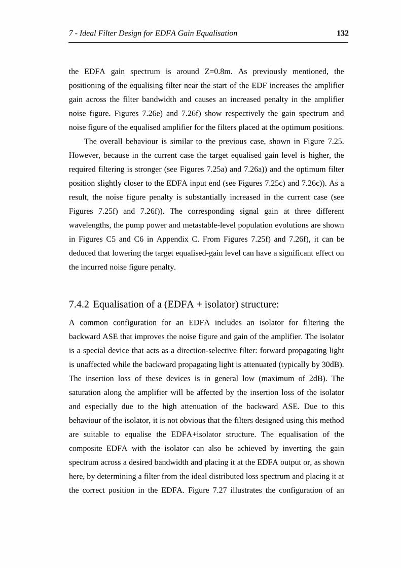
7-IdealFilterDesignforEDFAGainEqualisation 132
the EDFA gain spectrum is around Z=0.8m. As previously mentioned, the
positioningoftheequalisingfilternearthestartoftheEDFincreasestheamplifier
gain across the filter bandwidth and causes an increased penalty in the amplifier
noise figure. Figures 7.26e) and 7.26f) show respectively the gain spectrum and
noisefigureoftheequalisedamplifierforthefiltersplacedattheoptimumpositions.
The overall behaviour is similar to the previous case, shown in Figure 7.25.
However, because in the current case the target equalisedgain level is higher, the
requiredfilteringisstronger(seeFigures7.25a)and7.26a))andtheoptimumfilter
positionslightlyclosertotheEDFAinputend(seeFigures7.25c)and7.26c)).Asa
result, the noise figure penalty is substantially increased in the current case (see
Figures 7.25f) and 7.26f)). The corresponding signal gain at three different
wavelengths,thepumppowerandmetastable-levelpopulationevolutionsareshown
in Figures C5 and C6 in Appendix C. From Figures 7.25f) and 7.26f), it can be
deducedthatloweringthetargetequalised-gainlevelcanhaveasignificanteffecton
theincurrednoisefigurepenalty.
7.4.2 Equalisationofa(EDFA+isolator)structure:
A common configuration for an EDFA includes an isolator for filtering the
backwardASEthatimprovesthenoisefigureandgainoftheamplifier.Theisolator
isaspecialdevicethatactsasadirection-selectivefilter:forwardpropagatinglight
isunaffectedwhilethebackwardpropagatinglightisattenuated(typicallyby30dB).
The insertion loss of these devices is in general low (maximum of 2dB). The
saturation along the amplifier will be affected by the insertion loss of the isolator
and especially due to the high attenuation of the backward ASE. Due to this
behaviouroftheisolator,itisnotobviousthatthefiltersdesignedusingthismethod
are suitable to equalise the EDFA+isolator structure. The equalisation of the
composite EDFA with the isolator can also be achieved by inverting the gain
spectrumacrossadesiredbandwidthandplacingitattheEDFAoutputor,asshown
here,bydeterminingafilterfromtheidealdistributedlossspectrumandplacingitat
the correct position in the EDFA. Figure 7.27 illustrates the configuration of an
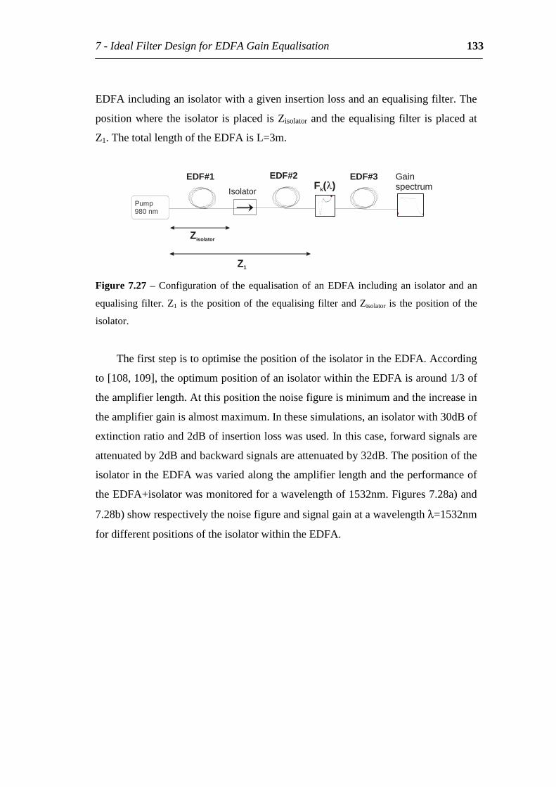
7-IdealFilterDesignforEDFAGainEqualisation 133
EDFAincludinganisolatorwithagiveninsertionlossandanequalisingfilter.The
positionwhere the isolator isplaced isZisolatorand theequalisingfilter isplacedat
Z1.ThetotallengthoftheEDFAisL=3m.
Pump980nm
Zisolator
Z1
EDF#1 EDF#2 EDF#3F ( )k λ
GainspectrumIsolator
Figure7.27–Configurationof theequalisationofanEDFAincludingan isolatorandan
equalisingfilter.Z1 is thepositionof theequalisingfilterandZisolator is thepositionofthe
isolator.
ThefirststepistooptimisethepositionoftheisolatorintheEDFA.According
to[108,109],theoptimumpositionofanisolatorwithintheEDFAisaround1/3of
theamplifierlength.Atthispositionthenoisefigureisminimumandtheincreasein
theamplifiergainisalmostmaximum.Inthesesimulations,anisolatorwith30dBof
extinctionratioand2dBofinsertionlosswasused.Inthiscase,forwardsignalsare
attenuatedby2dBandbackwardsignalsareattenuatedby32dB.Thepositionofthe
isolatorintheEDFAwasvariedalongtheamplifierlengthandtheperformanceof
theEDFA+isolatorwasmonitoredforawavelengthof1532nm.Figures7.28a)and
7.28b)showrespectivelythenoisefigureandsignalgainatawavelengthλ=1532nm
fordifferentpositionsoftheisolatorwithintheEDFA.
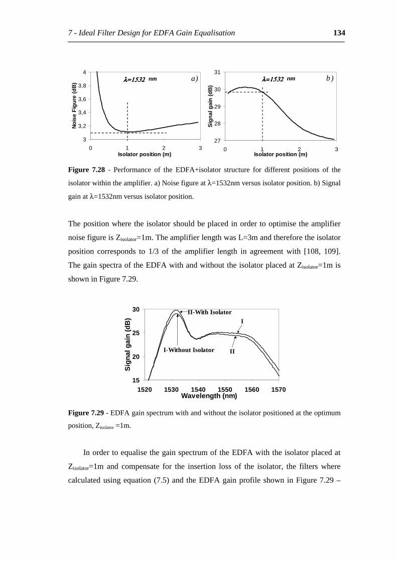
7-IdealFilterDesignforEDFAGainEqualisation 134
3
3,2
3,4
3,6
3,8
4
0 1 2 3Isolatorposition(m)
Noi
seF
igur
e(d
B)
a)λ=1532λ=1532λ=1532λ=1532 nm
27
28
29
30
31
0 1 2 3Isolatorposition(m)
Sig
nalg
ain
(dB
)
b)λ=1532λ=1532λ=1532λ=1532 nm
Figure 7.28 - Performance of the EDFA+isolator structure for different positions of the
isolatorwithintheamplifier.a)Noisefigureatλ=1532nmversusisolatorposition.b)Signal
gainatλ=1532nmversusisolatorposition.
Thepositionwheretheisolatorshouldbeplacedinorder tooptimisetheamplifier
noisefigureisZisolator=1m.TheamplifierlengthwasL=3mandthereforetheisolator
position corresponds to 1/3 of the amplifier length in agreement with [108, 109].
ThegainspectraoftheEDFAwithandwithouttheisolatorplacedatZisolator=1mis
showninFigure7.29.
15
20
25
30
1520 1530 1540 1550 1560 1570Wavelength(nm)
Sig
nalg
ain
(dB
)
II-WithIsolator
I-WithoutIsolator II
I
Figure7.29-EDFAgainspectrumwithandwithouttheisolatorpositionedattheoptimum
position,Zisolator=1m.
InordertoequalisethegainspectrumoftheEDFAwiththeisolatorplacedat
Zisolator=1m and compensate for the insertion loss of the isolator, the filters where
calculatedusingequation(7.5)and theEDFAgainprofileshowninFigure7.29–
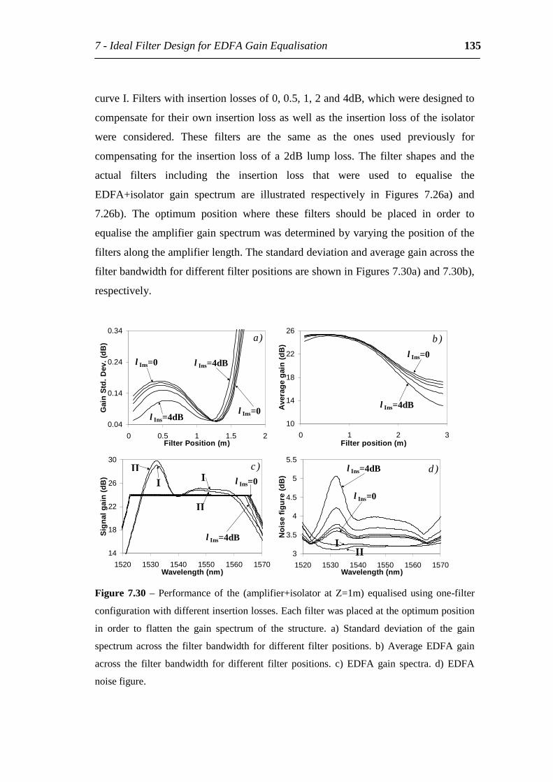
7-IdealFilterDesignforEDFAGainEqualisation 135
curveI.Filterswithinsertionlossesof0,0.5,1,2and4dB,whichweredesignedto
compensate for theirowninsertionlossaswellas theinsertionlossof theisolator
were considered. These filters are the same as the ones used previously for
compensating for the insertion loss of a 2dB lump loss. The filter shapes and the
actual filters including the insertion loss that were used to equalise the
EDFA+isolator gain spectrum are illustrated respectively in Figures 7.26a) and
7.26b). The optimum position where these filters should be placed in order to
equalisetheamplifiergainspectrumwasdeterminedbyvaryingthepositionofthe
filtersalongtheamplifierlength.Thestandarddeviationandaveragegainacrossthe
filterbandwidthfordifferentfilterpositionsareshowninFigures7.30a)and7.30b),
respectively.
0.04
0.14
0.24
0.34
0 0.5 1 1.5 2FilterPosition(m)
Gai
nS
td.D
ev.(
dB
) a)
l Ins=4dB
l Ins=0l Ins=4dB
l Ins=0
10
14
18
22
26
0 1 2 3Filterposition(m)
Ave
rag
eg
ain
(dB
)
b)l Ins=0
l Ins=4dB
14
18
22
26
30
1520 1530 1540 1550 1560 1570Wavelength(nm)
Sig
nalg
ain
(dB
)
c)
l Ins=4dB
l Ins=0
3
3.5
4
4.5
5
5.5
1520 1530 1540 1550 1560 1570Wavelength(nm)
Noi
sef
igu
re(d
B)
d)
l Ins=4dB
l Ins=0
Figure7.30–Performanceof the (amplifier+isolator atZ=1m)equalisedusingone-filter
configurationwithdifferentinsertionlosses.Eachfilterwasplacedattheoptimumposition
in order to flatten the gain spectrum of the structure. a) Standard deviation of the gain
spectrum across the filter bandwidth for different filter positions. b) Average EDFA gain
across the filter bandwidth for different filter positions. c) EDFA gain spectra. d) EDFA
noisefigure.
7-IdealFilterDesignforEDFAGainEqualisation 136
FromFigure7.30a), theoptimumfilterpositionisaroundZ=1.2m(depending
onthefilterinsertionloss).Thesepositionsareclosetothemiddleoftheamplifier
andthereforeasmallpenaltyinthenoisefigureisobserved.
Theperformanceof the(EDFA+isolator+equalisingfilter)structurefor the
filters placed at the optimum positions is illustrated in Figures 7.30c) and 7.30d)
wheretheamplifiergainspectrumandnoisefigureareplottedrespectively.Forall
the filters, the amplifier gain spectrum is equalised and there is no penalty in the
averagegainasshowninFigure7.30c).Boththeinsertionlossofeachfilterandthe
insertionlossoftheisolatorwerecompensatedforbythefilterdesign.Thepositions
where the filtersareplaced inorder to flatten theamplifiergain spectrumcausea
small penalty in the amplifier noise figure, illustrated in Figure 7.30d). However
when using filtering devices with low insertion losses (below 1dB), a very low
amplifier noise figure can be obtained with gain spectrum equalisation and
compensationfortheisolatorinsertionloss.
Figures C7a), C7b) and C7c) in appendix C show the evolution of the signal
gain along the amplifier length for three different wavelengths, λ1=1532.3nm,
λ2=1539.4nmandλ3=1550.7nmrespectively.Thereisadropof2dBintheamplifier
gain corresponding to the insertion lossof the isolator atZ=1mandawavelength
dependentlossduetothefilterataround1.2m.Theamplifiergainpicksuptovalues
around24dBatallwavelengthsproducinganequalisedgainspectra.
Thewavelength-dependentnoisefigureshowninFigure7.30d)forthevarious
filtersisduetothedifferentevolutionofthesignalandforwardASEalongthefibre
length.TheforwardandbackwardASEpowerevolutionalongtheEDFlengthfor
different wavelengths is also illustrated in Figures C7d)-f). The power of the
backwardASEattheinputendoftheEDFAisverylowduetothepresenceofthe
isolator at Z=1m. Consequently, a lower pump absorption rate at the input of the
EDFA isobserved.Thepumppower andpopulation inversionalong the amplifier
lengthareillustratedinFiguresC8a)andC8b)respectively.Theisolatorpractically
doesnotaffectthepopulationinversionatZ=1mduetoitsrelativelylowinsertion
7-IdealFilterDesignforEDFAGainEqualisation 137
loss(2dB)butchangestheinitialpopulationinversionandpumpabsorptionatZ=0
duetotheattenuationof32dBinthebackwardASE.
7.4.3 Conclusions
ThedesignoffiltersforequalisingtheEDFAgainspectrumwhilecompensatingfor
their own insertion losses and thatofotherdeviceswas studied.The gainpenalty
duetotheinsertionofanarbitrarylossintheEDFcanbecompensatedforbymeans
of the calculation of the corrected filter shape and determination of the optimum
position.Howeverthereisapenaltyintheamplifiernoisefigureassociatedwiththe
incorporation of these filters in the amplifier. These novel filter designs can be
particularlyuseful incaseswherefilterswith intrinsicallyhigh insertion lossesare
used.
7.5 Summary
An approach for determining ideal wavelength-dependent loss filters and their
optimumpositioninordertoequalisetheEDFAgainspectrumwasdeveloped.One-
filter and two-filter equalisation schemes were compared: the first one is very
sensitive on the position where the filter is placed, and the second gives a good
approximation to a uniformly-distributed wavelength-dependent distributed loss,
insensitive to the exact placement of the filters. Different filter designs with or
without a correction for the device insertion losses, as well as filters obtained by
inverting the EDFA gain spectrum, were compared. Using filters that are not
designedtocompensatefortheinsertionlossesofthedevices,theirperformancein
flatteningtheEDFAgainspectrumissimilartofiltersobtainedusingtheinverseof
the amplifier gain and positioned at the output. When using filters designed to
correct for the respective insertion losses, gain equalisation is achieved with no
penaltyintheamplifiergainforfilterswithupto8dBinsertionlosses.However,in
7-IdealFilterDesignforEDFAGainEqualisation 138
thiscase,thereisaslightpenaltyintheamplifiernoisefigureduetothefactthatthe
optimum position where these filters are placed is closer to the input of the
amplifier.Thesummaryoftheperformanceofthesedifferentequalisationfiltersis
showninFigure7.22.
Themethodcanbeextendedtodesignfiltersthatcompensateforboththeirown
insertionlossandtheinsertionlossesofdifferentdevicesplacedalongtheamplifier.
Inparticulartwosituationswereaddressed;thefirstoneconsistedofequalisingthe
EDFA gain spectrum that included a loss element placed at Z=2m; the second to
equalisetheEFDAgainspectruminacommonlyusedconfigurationthatincludesan
optical isolator toavoidthebackwardASEbuildupwhile improvingbothitsgain
and noise figure. For both these situations the EDFA gain equalisation was
successful using one equalising filter and the correct filter design and placement
withintheamplifier.
Finally,tunablefilters,similartotheonesdemonstratedinthepreviouschapter,
could be designed using the calculated ideal filter shapes in order to dynamically
equalisetheEDFAgainspectrum.Alternatively,asthistheoryisvalidforarbitrary
EDFA saturations (including pumping conditions and signal power), a range of
filterscouldbedesignedfordifferentsaturationconditionsandatunablefilterused
to scan among the possible configurations in order to equalise the EDFA gain
spectrumwithminimumcomputingtime.
8
All-FibreAdd-Drop
Multiplexers
InthisChapterall-fibreadd-dropmultiplexerconfigurationsbasedontheinscription
of Bragg gratings in the waist of fibre couplers are discussed. The main study is
aroundtheparametersinvolvedintheoptimisationofadesignbasedonahalf-cycle
coupler with a grating in its waist. A solution is presented in the form of a non-
uniform half-cycle coupler. This novel device is demonstrated experimentally and
shown tobe apotential solution for achieving the required specifications for add-
drop multiplexers in WDM systems. A new configuration based on a full-cycle
couplerwithagratinginscribedinitswaistisalsoanalysed.
8-All-FibreAdd-DropMultiplexers 140
8.1 Overview
Wavelength division multiplexing (WDM) is one of the most important means of
obtaining high speed optical communications links. In these links, signals of
selectedwavelengthsneedtobedroppedoraddedtotheopticalstreamatdifferent
pointsalongthenetwork.Severaladd-dropmultiplexerschemeshavebeenreported
in the literature. Planar devices based on gratings in coupler structures present
compact and efficient solutions to the problem. However, these devices have
intrinsicproblemslikepolarisationsensitivityandhighinsertionlosses.Severaladd-
dropmultiplexerdevicesbasedonall-fibreschemeshavebeenextensivelyanalysed
asmentionedinChapter4.
Aparticularfamilyofall-fibreadd-dropmultiplexersisbasedontheinscription
ofBragggratingsinthewaistoffibre-couplers.Theinscriptionofatiltedgratingin
the waist of a null coupler has been demonstrated as suitable for add-drop
performance[39,110]. Inthischapter thefocus isonadd-dropmultiplexersbased
on the inscription of gratings in the waist of half-cycle and full-cycle couplers.
Design considerations and parameters to be optimised are analysed and a novel
design based on a non-uniform half-cycle coupler is presented as an optimised
solution.
8.2 NumericalModel
The performance of add-drop multiplexers based on the inscription of a Bragg
grating in the waist of a fibre coupler can be simulated using the transfer matrix
approachforthewholestructure.Thepropagatingevenandoddcouplereigenmodes
withpropagationconstantsβeandβo,respectively,arereflectedindividuallybythe
grating.Both the reflected lightarrivingat the inputportand the transmitted light
arrivingattheoutputportsaredecomposedintothenormalmodesoftheindividual
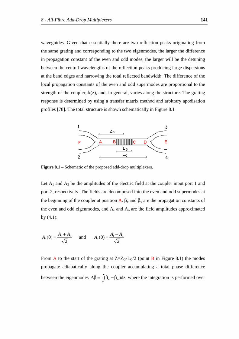
8-All-FibreAdd-DropMultiplexers 141
waveguides. Given that essentially there are two reflectionpeaksoriginating from
thesamegratingandcorrespondingtothetwoeigenmodes,thelargerthedifference
inpropagationconstantoftheevenandoddmodes,thelargerwillbethedetuning
betweenthecentralwavelengthsofthereflectionpeaksproducinglargedispersions
atthebandedgesandnarrowingthetotalreflectedbandwidth.Thedifferenceofthe
localpropagationconstantsoftheevenandoddsupermodesareproportionaltothe
strengthofthecoupler,k(z),and,ingeneral,variesalongthestructure.Thegrating
responseisdeterminedbyusingatransfermatrixmethodandarbitraryapodisation
profiles[78].ThetotalstructureisshownschematicallyinFigure8.1
Figure8.1–Schematicoftheproposedadd-dropmultiplexers.
LetA1andA2betheamplitudesoftheelectricfieldatthecouplerinputport1and
port2,respectively.Thefieldsaredecomposedintotheevenandoddsupermodesat
thebeginningofthecoupleratpositionA.βeandβoarethepropagationconstantsof
theevenandoddeigenmodes,andAeandAoarethefieldamplitudesapproximated
by(4.1):
2)0( 21 AA
Ae
+= and2
)0( 21 AAAo
−=
FromAtothestartof thegratingatZ=ZG-LG/2(pointBinFigure8.1) themodes
propagate adiabatically along the coupler accumulating a total phase difference
betweentheeigenmodes β−β=β∆z
0 oe dz)( wheretheintegrationisperformedover
8-All-FibreAdd-DropMultiplexers 142
the travelled distance. At B the fields of the forward propagating even and odd
eigenmodesaregivenby:
=−
−
−2/
0
,
)0()2/( ,,
GLGZ
oe dzi
oeGGoe eALZEβ
(8.1)
The reflected field for the even and odd eigenmodes is given by multiplying the
gratingreflectioncoefficient,ρe,o(0),bytherespectiveelectricfieldatthestartofthe
grating.DenominatingEe’ andEo’ thefieldsofthebackwardpropagatingevenand
oddeigenmodesrespectively,atthestartofthegratingtheycanbewrittenas
)2/()2/(' ,,, GGoeoeGGoe LZELZE −=− ρ (8.2)
andatthestartofthecoupler(positionA),thefieldsofthebackwardreflectedeven
andoddeigenmodesarewrittenas,
=
−
−2/
0
,2
,,, )0()0('
GLGZ
oe dzi
oeoeoe eAEβ
ρ (8.3)
The phase of the reflected even and odd eigenmodes depends now on both the
propagation along the coupler and the phase due to the corresponding complex
reflectivityof thegrating.The light transmitted through thegrating isobtainedby
multiplying the transmission coefficient, t(LG) by the fields at the input of the
grating.AtpositionCcorresponding toZ=ZG+LG/2, theforwardpropagatingeven
andoddmodefieldscanbewrittenas
=+
−
−2/
0
,
,,, )0()2/(
GLGZ
oe dzi
oeoeGGoe etALZEβ
(8.4)

8-All-FibreAdd-DropMultiplexers 143
The expressions for the electric fields of the forward propagating even and odd
eigenmodesattheendofthecoupler(positionD)arewrittenas:
+−
= +
− CZ
GLGZ
oe
GLGZ
oe dzdzi
oeoeCoe etALE 2/
,
2/
0
,
,,, )0()(ββ
(8.5)
The spectral properties of the grating namely the transmission and reflection
coefficients are obtained by using a transfer matrix model [78] by dividing the
grating into N uniform sections and multiplying the transfer functions of each
section.Toobtainthelightpowerarrivingateachoneoftheports,theevenandodd
mode fields are decomposed into the fields of the normal waveguides using
expression (4.1). The response of the grating written within the coupler waist in
general differs from the performance of the device itself due to the difference in
propagationconstantsbetweentheevenandoddeigenmodes.
8.3 Add-DropConfigurations
Devicesthatrelyontheinscriptionofnon-tiltedBragggratingsinthewaistoffibre
couplers are studied. Three different add-drop multiplexer configurations are
analysedandcompared.
The first design relieson agratingwritten in ahalf-cycle fused fibre coupler.
Thisdevicehasbeendemonstrated[42]byplacingagratingatthecentreofafused-
coupler waist and, by writing identical gratings in two separate fibres and then
polishedtogetherformingalongcouplingregion[111].Severalissuesrelatedtothe
optimisationandperformanceofthisdeviceareevaluatedinthischapter.Theeffect
of the difference in propagation constant of the coupler eigenmodes, the grating
apodisationandlength,thepenetrationdepthoftheradiationintheBragggratings
and the position within the couplers where they should be placed are addressed.
Experimentalaspectsthatmaydegradethedeviceperformancearealsodiscussed.
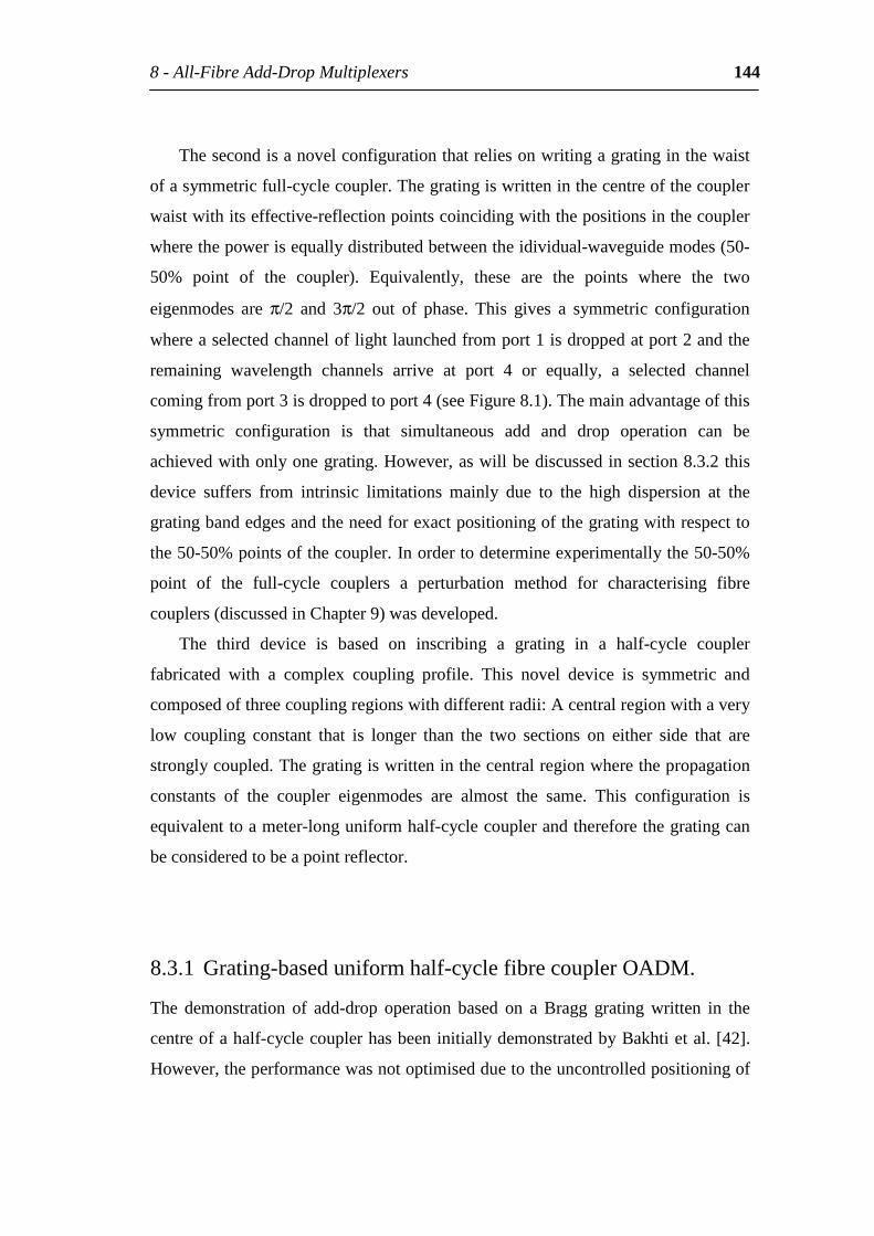
8-All-FibreAdd-DropMultiplexers 144
Thesecondisanovelconfigurationthatreliesonwritingagratinginthewaist
ofasymmetricfull-cyclecoupler.Thegratingiswritteninthecentreofthecoupler
waistwithitseffective-reflectionpointscoincidingwiththepositionsinthecoupler
wherethepowerisequallydistributedbetweentheidividual-waveguidemodes(50-
50% point of the coupler). Equivalently, these are the points where the two
eigenmodes are π/2 and 3π/2 out of phase. This gives a symmetric configuration
whereaselectedchanneloflightlaunchedfromport1isdroppedatport2andthe
remaining wavelength channels arrive at port 4 or equally, a selected channel
comingfromport3isdroppedtoport4(seeFigure8.1).Themainadvantageofthis
symmetric configuration is that simultaneous add and drop operation can be
achievedwithonlyonegrating.However,aswillbediscussedinsection8.3.2this
device suffers from intrinsic limitations mainly due to the high dispersion at the
gratingbandedgesandtheneedforexactpositioningofthegratingwithrespectto
the50-50%pointsofthecoupler.Inordertodetermineexperimentallythe50-50%
point of the full-cycle couplers a perturbation method for characterising fibre
couplers(discussedinChapter9)wasdeveloped.
The third device is based on inscribing a grating in a half-cycle coupler
fabricated with a complex coupling profile. This novel device is symmetric and
composedofthreecouplingregionswithdifferentradii:Acentralregionwithavery
low coupling constant that is longer than the two sections on either side that are
stronglycoupled.Thegratingiswritteninthecentralregionwherethepropagation
constants of the coupler eigenmodes are almost the same. This configuration is
equivalenttoameter-longuniformhalf-cyclecouplerandthereforethegratingcan
beconsideredtobeapointreflector.
8.3.1 Grating-baseduniformhalf-cyclefibrecouplerOADM.
The demonstration of add-drop operation based on a Bragg grating written in the
centreofahalf-cyclecouplerhasbeeninitiallydemonstratedbyBakhtietal.[42].
However,theperformancewasnotoptimisedduetotheuncontrolledpositioningof
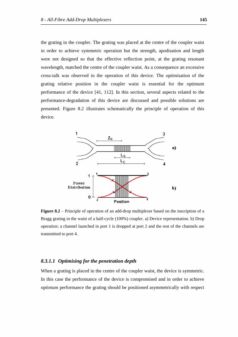
8-All-FibreAdd-DropMultiplexers 145
thegratinginthecoupler.Thegratingwasplacedatthecentreofthecouplerwaist
in order to achieve symmetric operation but the strength, apodisation and length
were not designed so that the effective reflection point, at the grating resonant
wavelength,matchedthecentreofthecouplerwaist.Asaconsequenceanexcessive
cross-talk was observed in the operation of this device. The optimisation of the
grating relative position in the coupler waist is essential for the optimum
performanceof thedevice [41,112]. In this section, several aspects related to the
performance-degradation of this device are discussed and possible solutions are
presented. Figure 8.2 illustrates schematically the principle of operation of this
device.
Figure8.2–Principleofoperationofanadd-dropmultiplexerbasedontheinscriptionofa
Bragggratinginthewaistofahalf-cycle(100%)coupler.a)Devicerepresentation.b)Drop
operation:achannellaunchedinport1isdroppedatport2andtherestofthechannelsare
transmittedtoport4.
8.3.1.1 Optimisingforthepenetrationdepth
Whenagratingisplacedinthecentreofthecouplerwaist,thedeviceissymmetric.
Inthiscasetheperformanceof thedeviceiscompromisedandinorder toachieve
optimumperformancethegratingshouldbepositionedasymmetricallywithrespect
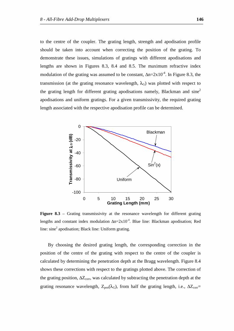
8-All-FibreAdd-DropMultiplexers 146
to the centre of the coupler. The grating length, strength and apodisation profile
should be taken into account when correcting the position of the grating. To
demonstrate these issues, simulations of gratings with different apodisations and
lengths are shown in Figures 8.3, 8.4 and 8.5. The maximum refractive index
modulationofthegratingwasassumedtobeconstant,∆n=2x10⁻⁴.InFigure8.3,the
transmission (at thegrating resonancewavelength,λG)wasplottedwithrespect to
the grating length for different grating apodisations namely, Blackman and sine2
apodisationsanduniformgratings.For agiven transmissivity, the requiredgrating
lengthassociatedwiththerespectiveapodisationprofilecanbedetermined.
-100
-80
-60
-40
-20
0
0 5 10 15 20 25 30GratingLength(mm)
Tran
smis
sivi
tya
t λλ λλG(d
B)
Uniform
Blackman
Sin2(x)
Figure 8.3 – Grating transmissivity at the resonance wavelength for different grating
lengths and constant index modulation ∆n=2x10⁻⁴. Blue line: Blackman apodisation; Red
line:sine2apodisation;Blackline:Uniformgrating.
By choosing the desired grating length, the corresponding correction in the
position of the centre of the grating with respect to the centre of the coupler is
calculatedbydeterminingthepenetrationdepthattheBraggwavelength.Figure8.4
showsthesecorrectionswithrespecttothegratingsplottedabove.Thecorrectionof
thegratingposition,∆Zcorr,wascalculatedbysubtractingthepenetrationdepthatthe
grating resonance wavelength, Zpen(λG), from half the grating length, i.e., ∆Zcorr=
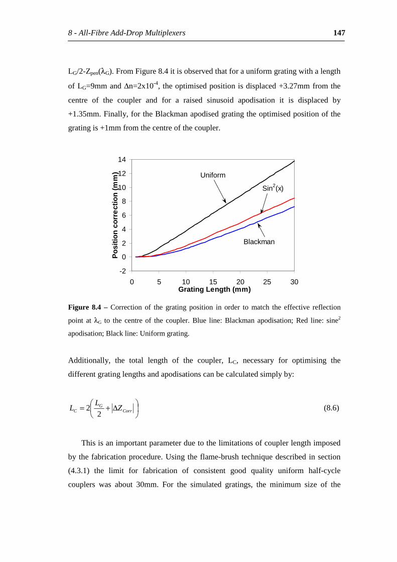
8-All-FibreAdd-DropMultiplexers 147
LG/2-Zpen(λG).FromFigure8.4itisobservedthatforauniformgratingwithalength
ofLG=9mmand∆n=2x10⁻⁴, theoptimisedpositionisdisplaced+3.27mmfromthe
centre of the coupler and for a raised sinusoid apodisation it is displaced by
+1.35mm.Finally,fortheBlackmanapodisedgratingtheoptimisedpositionofthe
gratingis+1mmfromthecentreofthecoupler.
-2
0
2
4
6
8
10
12
14
0 5 10 15 20 25 30GratingLength(mm)
Pos
ition
cor
rect
ion
(mm
) Uniform
Blackman
Sin2(x)
Figure 8.4 – Correction of the grating position in order to match the effective reflection
point atλG to the centreof the coupler. Blue line: Blackman apodisation; Red line: sine2
apodisation;Blackline:Uniformgrating.
Additionally, the total length of the coupler, LC, necessary for optimising the
differentgratinglengthsandapodisationscanbecalculatedsimplyby:
∆+= CorrG
C ZL
L2
2 (8.6)
Thisisanimportantparameterduetothelimitationsofcouplerlengthimposed
bythefabricationprocedure.Usingtheflame-brushtechniquedescribed insection
(4.3.1) the limit for fabrication of consistent good quality uniform half-cycle
couplers was about 30mm. For the simulated gratings, the minimum size of the
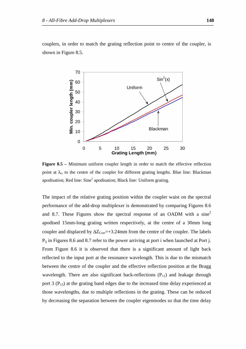
8-All-FibreAdd-DropMultiplexers 148
couplers, inorder tomatch thegrating reflectionpoint to centreof the coupler, is
showninFigure8.5.
0
10
20
30
40
50
60
70
0 5 10 15 20 25 30GratingLength(mm)
Min
.cou
pler
leng
th(m
m)
Uniform
Blackman
Sin2(x)
Figure 8.5 – Minimum uniform coupler length in order to match the effective reflection
point atλG to the centreof the coupler fordifferentgrating lengths.Blue line:Blackman
apodisation;Redline:Sine2apodisation;Blackline:Uniformgrating.
Theimpactof therelativegratingpositionwithinthecouplerwaistonthespectral
performanceoftheadd-dropmultiplexerisdemonstratedbycomparingFigures8.6
and 8.7. These Figures show the spectral response of an OADM with a sine2
apodised 15mm-long grating written respectively, at the centre of a 30mm long
coupleranddisplacedby∆ZCorr=+3.24mmfromthecentreofthecoupler.Thelabels
PijinFigures8.6and8.7refertothepowerarrivingatportiwhenlaunchedatPortj.
From Figure 8.6 it is observed that there is a significant amount of light back
reflectedtotheinputportattheresonancewavelength.Thisisduetothemismatch
betweenthecentreof thecouplerandtheeffectivereflectionpositionattheBragg
wavelength. There are also significant back-reflections (P11) and leakage through
port3(P13)atthegratingbandedgesduetotheincreasedtimedelayexperiencedat
thosewavelengths,duetomultiplereflectionsinthegrating.Thesecanbereduced
bydecreasingtheseparationbetweenthecouplereigenmodessothatthetimedelay
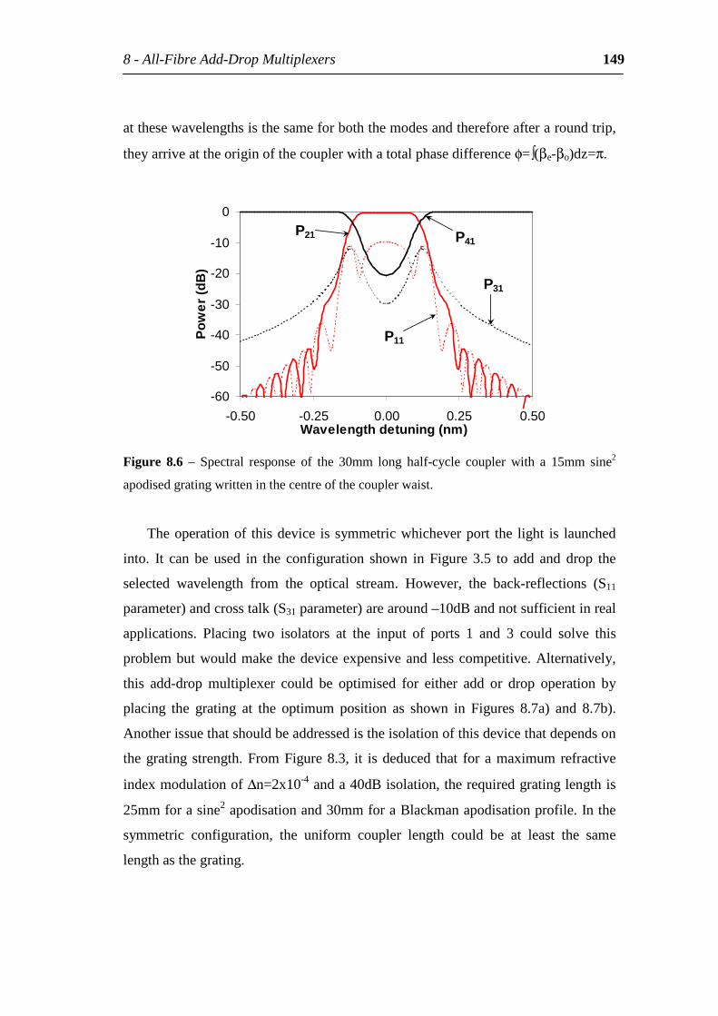
8-All-FibreAdd-DropMultiplexers 149
atthesewavelengthsisthesameforboththemodesandthereforeafteraroundtrip,
theyarriveattheoriginofthecouplerwithatotalphasedifferenceφ=(βe-βo)dz=π.
-60
-50
-40
-30
-20
-10
0
-0.50 -0.25 0.00 0.25 0.50Wavelengthdetuning(nm)
Pow
er(d
B)
P11
P21 P41
P31
Figure 8.6 – Spectral response of the 30mm long half-cycle coupler with a 15mm sine2
apodisedgratingwritteninthecentreofthecouplerwaist.
Theoperationof thisdevice issymmetricwhicheverport the light is launched
into. It can be used in the configuration shown in Figure 3.5 to add and drop the
selected wavelength from the optical stream. However, the back-reflections (S11
parameter)andcrosstalk(S31parameter)arearound–10dBandnotsufficientinreal
applications. Placing two isolators at the input of ports 1 and 3 could solve this
problembutwouldmake thedeviceexpensiveand lesscompetitive.Alternatively,
this add-drop multiplexer could be optimised for either add or drop operation by
placing the grating at the optimum position as shown in Figures 8.7a) and 8.7b).
Anotherissuethatshouldbeaddressedistheisolationofthisdevicethatdependson
thegratingstrength.FromFigure8.3, it isdeduced that foramaximumrefractive
indexmodulationof∆n=2x10⁻⁴anda40dBisolation,therequiredgratinglengthis
25mmforasine2apodisationand30mmforaBlackmanapodisationprofile.Inthe
symmetric configuration, the uniform coupler length could be at least the same
lengthasthegrating.
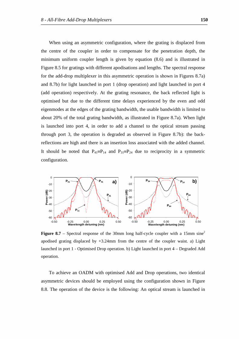
8-All-FibreAdd-DropMultiplexers 150
Whenusingan asymmetric configuration,where thegrating isdisplaced from
the centre of the coupler in order to compensate for the penetration depth, the
minimum uniform coupler length is given by equation (8.6) and is illustrated in
Figure8.5forgratingswithdifferentapodisationsandlengths.Thespectralresponse
fortheadd-dropmultiplexerinthisasymmetricoperationisshowninFigures8.7a)
and8.7b)forlightlaunchedinport1(dropoperation)andlightlaunchedinport4
(add operation) respectively. At the grating resonance, the back reflected light is
optimised but due to the different time delays experienced by the even and odd
eigenmodesattheedgesofthegratingbandwidth,theusablebandwidthislimitedto
about20%ofthetotalgratingbandwidth,asillustratedinFigure8.7a).Whenlight
is launched into port 4, in order to add a channel to the optical stream passing
through port 3, the operation is degraded as observed in Figure 8.7b): the back-
reflectionsarehighandthereisaninsertionlossassociatedwiththeaddedchannel.
It should be noted that P41≡P14 and P31≡P24 due to reciprocity in a symmetric
configuration.
-60
-50
-40
-30
-20
-10
0
-0.50 -0.25 0.00 0.25 0.50Wavelengthdetuning(nm)
Pow
er(d
B)
P11
P21 P41
P31
a)
-60
-50
-40
-30
-20
-10
0
-0.50 -0.25 0.00 0.25 0.50Wavelengthdetuning(nm)
Pow
er(d
B)
P44
P34 P14
P24
b)
Figure 8.7 – Spectral response of the 30mm long half-cycle coupler with a 15mm sine2
apodised grating displaced by +3.24mm from the centre of the coupler waist. a) Light
launchedinport1-OptimisedDropoperation.b)Lightlaunchedinport4–DegradedAdd
operation.
ToachieveanOADMwithoptimisedAddandDropoperations, two identical
asymmetric devices should be employed using the configuration shown in Figure
8.8.Theoperationof thedeviceis thefollowing:Anopticalstreamis launchedin
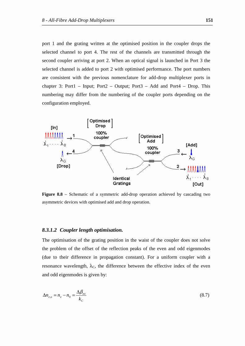
8-All-FibreAdd-DropMultiplexers 151
port 1 and the grating written at the optimised position in the coupler drops the
selected channel to port 4. The rest of the channels are transmitted through the
secondcouplerarrivingatport2.Whenanopticalsignal is launchedinPort3the
selectedchannel isaddedtoport2withoptimisedperformance.Theportnumbers
are consistent with the previous nomenclature for add-drop multiplexer ports in
chapter 3: Port1 – Input; Port2 – Output; Port3 – Add and Port4 – Drop. This
numbering may differ from the numbering of the coupler ports depending on the
configurationemployed.
Figure 8.8 – Schematic of a symmetric add-drop operation achieved by cascading two
asymmetricdeviceswithoptimisedaddanddropoperation.
8.3.1.2 Couplerlengthoptimisation.
Theoptimisationof thegratingposition in thewaistof thecouplerdoesnotsolve
the problem of the offset of the reflection peaks of the even and odd eigenmodes
(due to their difference in propagation constant). For a uniform coupler with a
resonance wavelength, λC, the difference between the effective index of the even
andoddeigenmodesisgivenby:
C
eoeoe k
nnnβ∆=−=∆ 0, (8.7)
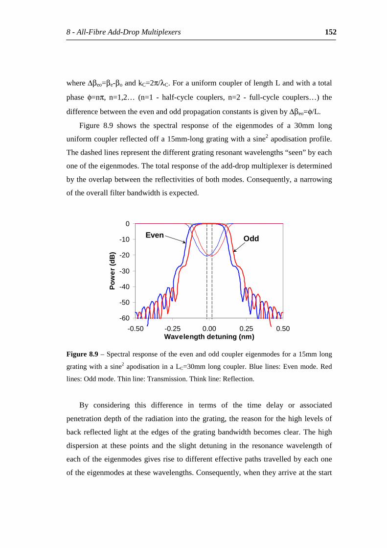
8-All-FibreAdd-DropMultiplexers 152
where∆βeo=βe-βoandkC=2π/λC.ForauniformcoupleroflengthLandwithatotal
phase φ=nπ, n=1,2… (n=1 - half-cycle couplers, n=2 - full-cycle couplers…) the
differencebetweentheevenandoddpropagationconstantsisgivenby∆βeo=φ/L.
Figure 8.9 shows the spectral response of the eigenmodes of a 30mm long
uniformcouplerreflectedoffa15mm-longgratingwithasine2apodisationprofile.
Thedashedlinesrepresentthedifferentgratingresonantwavelengths“seen”byeach
oneoftheeigenmodes.Thetotalresponseoftheadd-dropmultiplexerisdetermined
bytheoverlapbetweenthereflectivitiesofbothmodes.Consequently,anarrowing
oftheoverallfilterbandwidthisexpected.
-60
-50
-40
-30
-20
-10
0
-0.50 -0.25 0.00 0.25 0.50Wavelengthdetuning(nm)
Pow
er(d
B)
Even Odd
Figure8.9–Spectralresponseoftheevenandoddcouplereigenmodesfora15mmlong
gratingwithasine2apodisation inaLC=30mmlongcoupler.Blue lines:Evenmode.Red
lines:Oddmode.Thinline:Transmission.Thinkline:Reflection.
By considering this difference in terms of the time delay or associated
penetrationdepthoftheradiationintothegrating,thereasonforthehighlevelsof
backreflectedlightat theedgesof thegratingbandwidthbecomesclear.Thehigh
dispersion at these points and the slight detuning in the resonance wavelength of
eachoftheeigenmodesgivesrisetodifferenteffectivepathstravelledbyeachone
oftheeigenmodesatthesewavelengths.Consequently,whentheyarriveatthestart
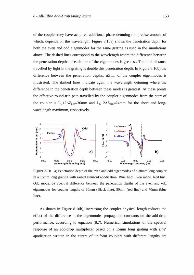
8-All-FibreAdd-DropMultiplexers 153
of thecoupler theyhaveacquiredadditionalphasedetuning thepreciseamountof
which, depends on the wavelength. Figure 8.10a) shows the penetration depth for
both theevenandoddeigenmodesfor thesamegratingasused in thesimulations
above.Thedashedlinescorrespondtothewavelengthwherethedifferencebetween
thepenetrationdepthsofeachoneoftheeigenmodesisgreatest.Thetotaldistance
travelledbylightinthegratingisdoublethispenetrationdepth.InFigure8.10b)the
difference between the penetration depths, ∆Zpen, of the coupler eigenmodes is
illustrated. The dashed lines indicate again the wavelength detuning where the
differenceinthepenetrationdepthbetweenthesemodesisgreatest.Atthesepoints
theeffective round-trippath travelledby thecouplereigenmodes from the startof
the coupler is LC+2∆Zpen≈36mm and LC+2∆Zpen≈24mm for the short and long-
wavelengthmaximum,respectively.
4
5
6
7
8
9
10
11
-0.50 -0.25 0.00 0.25 0.50Wavelengthdetuning(nm)
Pen
etra
tion
dept
h(m
m)
Even
Odd
a)-3
-2
-1
0
1
2
3
-0.50 -0.25 0.00 0.25 0.50Wavelengthdetuning(nm)
∆∆ ∆∆Z p
en(m
m)
b)
LC=30mm
LC=50mm
LC=70mm
Figure8.10–a)Penetrationdepthoftheevenandoddeigenmodesofa30mmlongcoupler
ina15mmlonggratingwithraisedsinusoidapodisation.Blueline:Evenmode.Redline:
Odd mode. b) Spectral difference between the penetration depths of the even and odd
eigenmodes for coupler lengths of 30mm (Black line), 50mm (red line) and 70mm (blue
line).
As shown inFigure8.10b), increasing thecouplerphysical length reduces the
effect of the difference in the eigenmodes propagation constants on the add-drop
performance, according to equation (8.7). Numerical simulations of the spectral
response of an add-drop multiplexer based on a 15mm long grating with sine2
apodisation written in the centre of uniform couplers with different lengths are
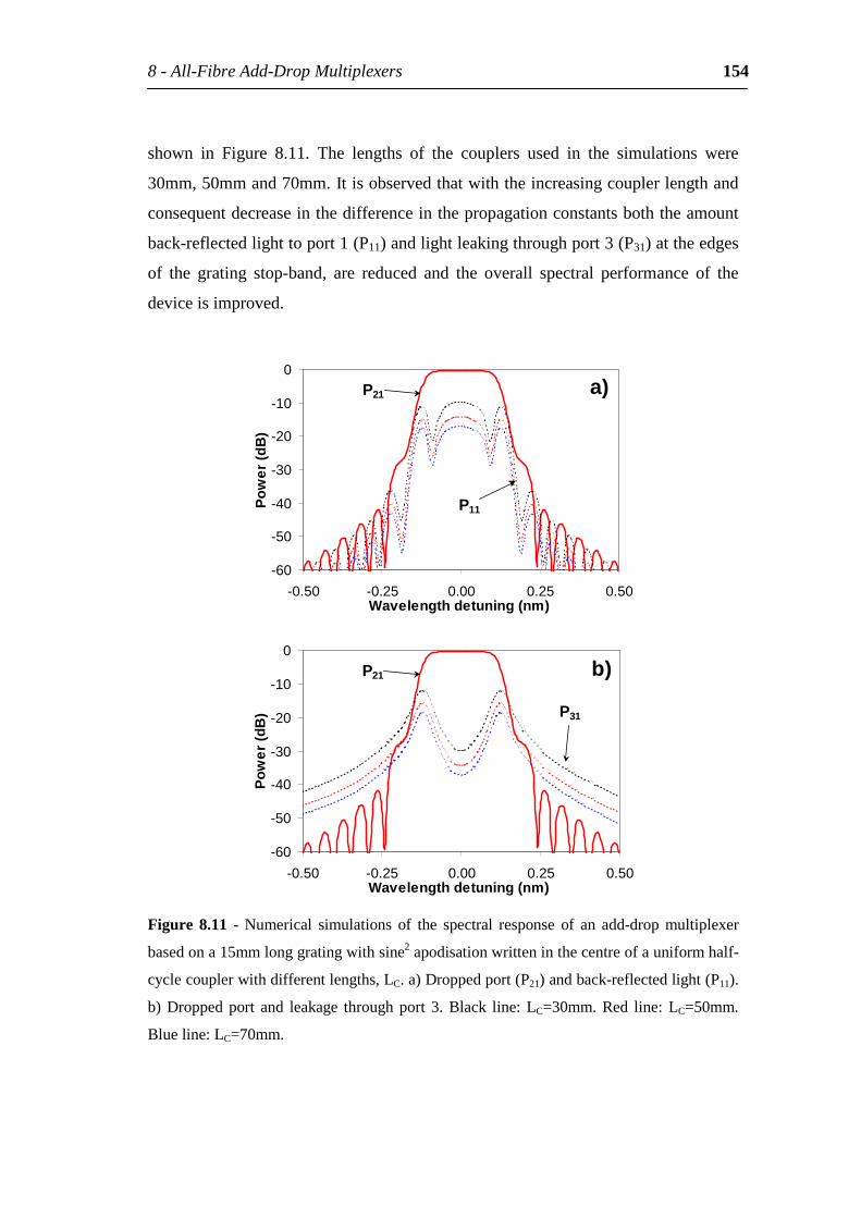
8-All-FibreAdd-DropMultiplexers 154
shown in Figure 8.11. The lengths of the couplers used in the simulations were
30mm,50mmand70mm.Itisobservedthatwiththeincreasingcouplerlengthand
consequentdecreaseinthedifferenceinthepropagationconstantsboththeamount
back-reflectedlighttoport1(P11)andlightleakingthroughport3(P31)attheedges
of the grating stop-band, are reduced and the overall spectral performance of the
deviceisimproved.
-60
-50
-40
-30
-20
-10
0
-0.50 -0.25 0.00 0.25 0.50Wavelengthdetuning(nm)
Pow
er(d
B)
P11
P21 a)
-60
-50
-40
-30
-20
-10
0
-0.50 -0.25 0.00 0.25 0.50Wavelengthdetuning(nm)
Pow
er(d
B) P31
P21 b)
Figure 8.11 - Numerical simulations of the spectral response of an add-drop multiplexer
basedona15mmlonggratingwithsine2apodisationwritteninthecentreofauniformhalf-
cyclecouplerwithdifferentlengths,LC.a)Droppedport(P21)andback-reflectedlight(P11).
b)Droppedport and leakage throughport 3.Black line:LC=30mm.Red line:LC=50mm.
Blueline:LC=70mm.
8-All-FibreAdd-DropMultiplexers 155
Even for a coupler length of LC=70mm, the amount of back-reflections and light
leakingthroughport3attheedgesofthegratingbandwidtharestillaround-20dB.
Tofurtherincreasetheperformanceofthisdevice,thecouplerlengthshouldbethe
longestpossible.However,thecompactnessofthedeviceiscompromisedwhenthe
coupler length is increased and could give rise to stabilisation and packaging
problems. Furthermore, the fabrication of fused fibre-couplers with long uniform
waists isnot trivialand therefore this isaserious limitation to theperformanceof
this device. However, this device could be suitable for 50GHz channel spacing
across thegratingbandwidthwith thereducedrequirementof–20dBfordrop-port
and add-port isolations (see table A1 in appendix A). In order to overcome these
limitations a novel add-drop design was developed based on a non-uniform half-
cyclecoupler(section8.3.2).
8.3.1.3 Experiments
Experimentally,theprincipleofoptimisingoneoftheoperations(AddorDrop)by
displacing the grating from the centreof the coupler is shown.Thegrating length
was4mm-longandwithnoapodisation(uniform).Thegratingwaswrittenusingan
excimer laseroperating at193nm.TheUVbeamwasbroadenough to expose the
whole cross section of the coupler, which was oriented perpendicularly to the
incidentbeamsothatbothphotosensitiveareaswereequallyexposed.Thecoupler
was fabricated using a fibre with boron co-doped core and high NA. The coupler
was then loaded with hydrogen at 160bar for 15 days in order to increase the
photosensitivity to the UV radiation [84]. The coupler’ s spectral response was
measured both before loading with hydrogen and after the writing of the grating.
The reason for the choice of a boron co-doped fibre instead of fibres with a
photosensitivecladding,thatareusuallyusedtoincreasethephotosensitiveareawas
the poor coupler extinction ratios obtained when fabricating couplers with these
fibres[113].
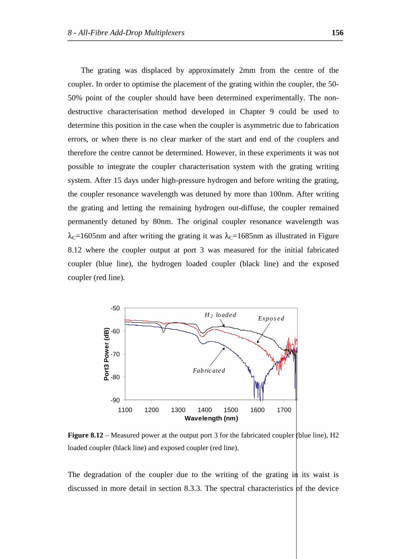
8-All-FibreAdd-DropMultiplexers 156
The grating was displaced by approximately 2mm from the centre of the
coupler.Inordertooptimisetheplacementofthegratingwithinthecoupler,the50-
50% point of the coupler should have been determined experimentally. The non-
destructive characterisation method developed in Chapter 9 could be used to
determinethispositioninthecasewhenthecouplerisasymmetricduetofabrication
errors, or when there is no clear marker of the start and end of the couplers and
thereforethecentrecannotbedetermined.However,intheseexperimentsitwasnot
possible to integrate the coupler characterisation system with the grating writing
system.After15daysunderhigh-pressurehydrogenandbeforewritingthegrating,
thecouplerresonancewavelengthwasdetunedbymorethan100nm.Afterwriting
the grating and letting the remaining hydrogen out-diffuse, the coupler remained
permanently detuned by 80nm. The original coupler resonance wavelength was
λC=1605nmandafterwritingthegratingitwasλC=1685nmasillustratedinFigure
8.12 where the coupler output at port 3 was measured for the initial fabricated
coupler (blue line), the hydrogen loaded coupler (black line) and the exposed
coupler(redline).
-90
-80
-70
-60
-50
1100 1200 1300 1400 1500 1600 1700Wavelength(nm)
Por
t3P
ower
(dB
)
Fabricated
ExposedH 2 loaded
Figure8.12–Measuredpowerattheoutputport3forthefabricatedcoupler(blueline),H2
loadedcoupler(blackline)andexposedcoupler(redline).
The degradation of the coupler due to the writing of the grating in its waist is
discussed inmoredetail insection8.3.3.Thespectralcharacteristicsof thedevice
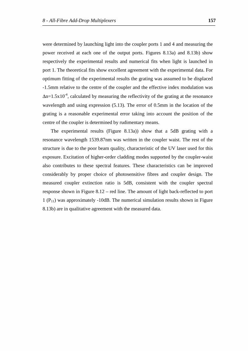
8-All-FibreAdd-DropMultiplexers 157
weredeterminedbylaunchinglightintothecouplerports1and4andmeasuringthe
power received at each one of the output ports. Figures 8.13a) and 8.13b) show
respectively the experimental results and numerical fits when light is launched in
port1.Thetheoreticalfitsshowexcellentagreementwiththeexperimentaldata.For
optimumfittingoftheexperimentalresultsthegratingwasassumedtobedisplaced
-1.5mmrelativetothecentreofthecouplerandtheeffectiveindexmodulationwas
∆n=1.5x10⁻⁴,calculatedbymeasuringthereflectivityofthegratingattheresonance
wavelengthandusingexpression(5.13).Theerrorof0.5mminthelocationof the
grating is a reasonable experimental error taking into account the position of the
centreofthecouplerisdeterminedbyrudimentarymeans.
The experimental results (Figure 8.13a)) show that a 5dB grating with a
resonancewavelength1539.87nmwaswritteninthecouplerwaist.Therestof the
structureisduetothepoorbeamquality,characteristicoftheUVlaserusedforthis
exposure.Excitationofhigher-ordercladdingmodessupportedbythecoupler-waist
also contributes to these spectral features. These characteristics can be improved
considerably by proper choice of photosensitive fibres and coupler design. The
measured coupler extinction ratio is 5dB, consistent with the coupler spectral
responseshowninFigure8.12–redline.Theamountoflightback-reflectedtoport
1(P11)wasapproximately-10dB.ThenumericalsimulationresultsshowninFigure
8.13b)areinqualitativeagreementwiththemeasureddata.
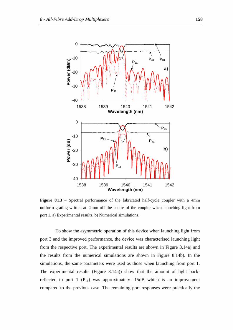
8-All-FibreAdd-DropMultiplexers 158
-40
-30
-20
-10
0
1538 1539 1540 1541 1542Wavelength(nm)
Pow
er(d
Bm
) P41 P31P21
P11
a)
-40
-30
-20
-10
0
1538 1539 1540 1541 1542Wavelength(nm)
Pow
er(d
B) P41
P31
P21
P11
b)
Figure 8.13 – Spectral performance of the fabricated half-cycle coupler with a 4mm
uniform grating written at -2mm off the centre of the coupler when launching light from
port1.a)Experimentalresults.b)Numericalsimulations.
Toshowtheasymmetricoperationofthisdevicewhenlaunchinglightfrom
port3andtheimprovedperformance,thedevicewascharacterisedlaunchinglight
from the respectiveport.The experimental resultsare shown inFigure8.14a)and
the results from the numerical simulations are shown in Figure 8.14b). In the
simulations, the sameparameterswereusedas thosewhen launching fromport1.
The experimental results (Figure 8.14a)) show that the amount of light back-
reflected to port 1 (P11) was approximately -15dB which is an improvement
compared to the previous case. The remaining port responses were practically the
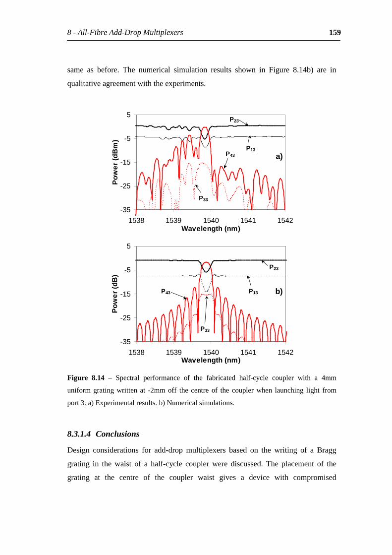
8-All-FibreAdd-DropMultiplexers 159
same as before. The numerical simulation results shown in Figure 8.14b) are in
qualitativeagreementwiththeexperiments.
-35
-25
-15
-5
5
1538 1539 1540 1541 1542Wavelength(nm)
Pow
er(d
Bm
)
P13
P23
P43
P33
a)
-35
-25
-15
-5
5
1538 1539 1540 1541 1542Wavelength(nm)
Pow
er(d
B)
P13
P23
P43
P33
b)
Figure 8.14 – Spectral performance of the fabricated half-cycle coupler with a 4mm
uniform grating written at -2mm off the centre of the coupler when launching light from
port3.a)Experimentalresults.b)Numericalsimulations.
8.3.1.4 Conclusions
Design considerations for add-drop multiplexers based on the writing of a Bragg
grating in the waist of a half-cycle coupler were discussed. The placement of the
grating at the centre of the coupler waist gives a device with compromised
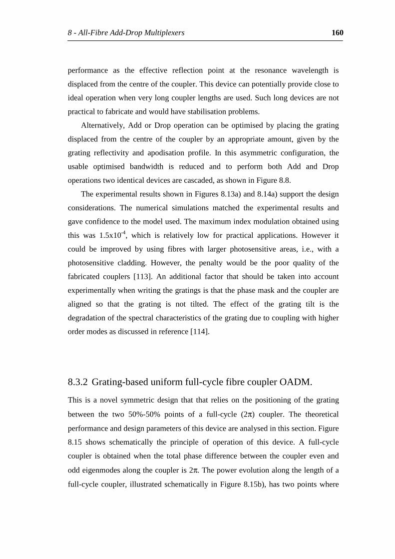
8-All-FibreAdd-DropMultiplexers 160
performance as the effective reflection point at the resonance wavelength is
displacedfromthecentreofthecoupler.Thisdevicecanpotentiallyprovidecloseto
idealoperationwhenverylongcouplerlengthsareused.Suchlongdevicesarenot
practicaltofabricateandwouldhavestabilisationproblems.
Alternatively, Add or Drop operation can be optimised by placing the grating
displaced from the centre of the coupler by an appropriate amount, given by the
grating reflectivity and apodisation profile. In this asymmetric configuration, the
usable optimised bandwidth is reduced and to perform both Add and Drop
operationstwoidenticaldevicesarecascaded,asshowninFigure8.8.
TheexperimentalresultsshowninFigures8.13a)and8.14a)supportthedesign
considerations. The numerical simulations matched the experimental results and
gaveconfidencetothemodelused.Themaximumindexmodulationobtainedusing
this was 1.5x10⁻⁴, which is relatively low for practical applications. However it
could be improved by using fibres with larger photosensitive areas, i.e., with a
photosensitive cladding. However, the penalty would be the poor quality of the
fabricated couplers [113]. An additional factor that should be taken into account
experimentallywhenwritingthegratingsisthatthephasemaskandthecouplerare
aligned so that the grating is not tilted. The effect of the grating tilt is the
degradationofthespectralcharacteristicsofthegratingduetocouplingwithhigher
ordermodesasdiscussedinreference[114].
8.3.2 Grating-baseduniformfull-cyclefibrecouplerOADM.
This is a novel symmetric design that that relies on the positioning of the grating
between the two 50%-50% points of a full-cycle (2π) coupler. The theoretical
performanceanddesignparametersofthisdeviceareanalysedinthissection.Figure
8.15 shows schematically the principle of operation of this device. A full-cycle
coupler is obtained when the total phase difference between the coupler even and
oddeigenmodesalongthecoupleris2π.Thepowerevolutionalongthelengthofa
full-cyclecoupler, illustratedschematically inFigure8.15b),has twopointswhere
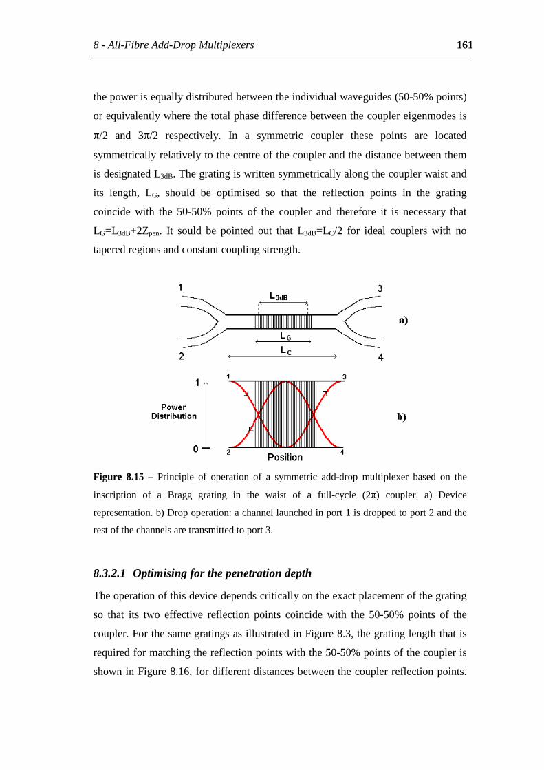
8-All-FibreAdd-DropMultiplexers 161
thepowerisequallydistributedbetweentheindividualwaveguides(50-50%points)
orequivalentlywherethetotalphasedifferencebetweenthecouplereigenmodesis
π/2 and 3π/2 respectively. In a symmetric coupler these points are located
symmetricallyrelativelytothecentreofthecouplerandthedistancebetweenthem
isdesignatedL3dB.Thegratingiswrittensymmetricallyalongthecouplerwaistand
its length, LG, should be optimised so that the reflection points in the grating
coincide with the 50-50% points of the coupler and therefore it is necessary that
LG=L3dB+2Zpen. It sould be pointed out that L3dB=LC/2 for ideal couplers with no
taperedregionsandconstantcouplingstrength.
Figure 8.15 – Principle of operation of a symmetric add-drop multiplexer based on the
inscription of a Bragg grating in the waist of a full-cycle (2π) coupler. a) Device
representation.b)Dropoperation:achannellaunchedinport1isdroppedtoport2andthe
restofthechannelsaretransmittedtoport3.
8.3.2.1 Optimisingforthepenetrationdepth
Theoperationofthisdevicedependscriticallyontheexactplacementofthegrating
so that its two effective reflection points coincide with the 50-50% points of the
coupler.ForthesamegratingsasillustratedinFigure8.3,thegratinglengththatis
requiredformatchingthereflectionpointswiththe50-50%pointsofthecoupleris
showninFigure8.16,fordifferentdistancesbetweenthecouplerreflectionpoints.
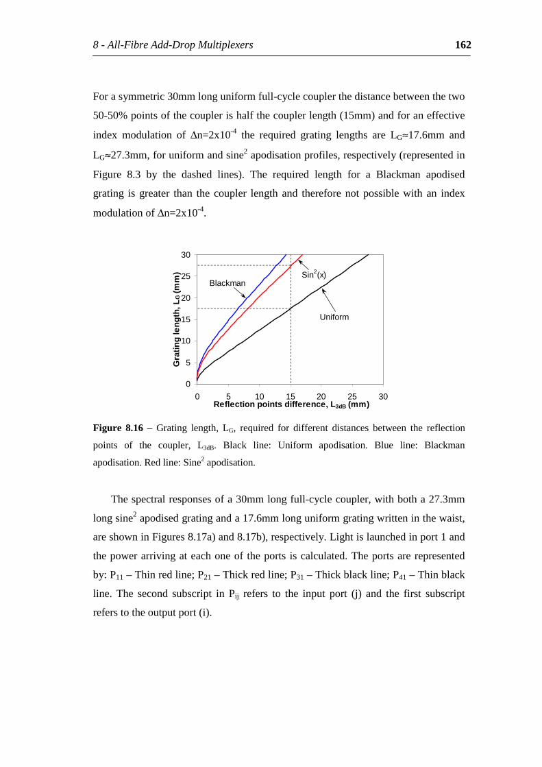
8-All-FibreAdd-DropMultiplexers 162
Forasymmetric30mmlonguniformfull-cyclecouplerthedistancebetweenthetwo
50-50%pointsofthecouplerishalfthecouplerlength(15mm)andforaneffective
index modulation of ∆n=2x10⁻⁴ the required grating lengths are LG≈17.6mm and
LG≈27.3mm,foruniformandsine2apodisationprofiles,respectively(representedin
Figure 8.3 by the dashed lines). The required length for a Blackman apodised
grating isgreater than the coupler length and thereforenotpossiblewith an index
modulationof∆n=2x10⁻⁴.
0
5
10
15
20
25
30
0 5 10 15 20 25 30Reflectionpointsdifference,L3dB(mm)
Gra
ting
leng
th,L
G(m
m)
Uniform
BlackmanSin2(x)
Figure 8.16 – Grating length, LG, required for different distances between the reflection
points of the coupler, L3dB. Black line: Uniform apodisation. Blue line: Blackman
apodisation.Redline:Sine2apodisation.
Thespectralresponsesofa30mmlongfull-cyclecoupler,withbotha27.3mm
longsine2apodisedgratinganda17.6mmlonguniformgratingwritteninthewaist,
areshowninFigures8.17a)and8.17b),respectively.Lightislaunchedinport1and
thepowerarrivingateachoneof theports iscalculated.Theportsarerepresented
by:P11–Thinredline;P21–Thickredline;P31–Thickblackline;P41–Thinblack
line. The second subscript in Pij refers to the input port (j) and the first subscript
referstotheoutputport(i).
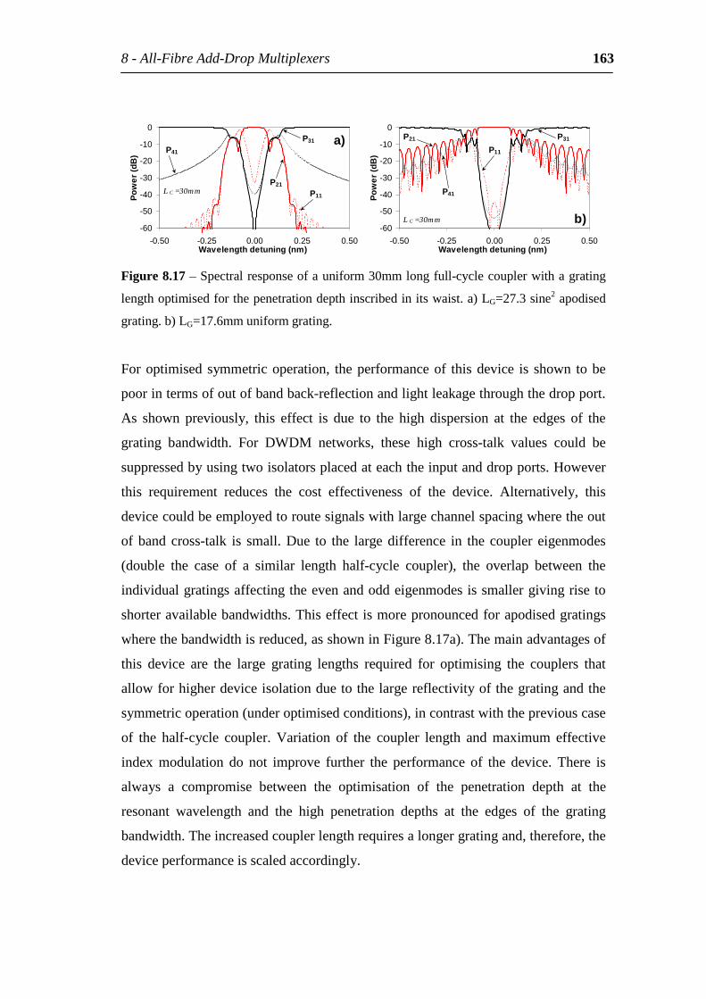
8-All-FibreAdd-DropMultiplexers 163
-60
-50
-40
-30
-20
-10
0
-0.50 -0.25 0.00 0.25 0.50Wavelengthdetuning(nm)
Pow
er(d
B)
P11
P21
P31
P41
L C =30mm
a)
-60
-50
-40
-30
-20
-10
0
-0.50 -0.25 0.00 0.25 0.50Wavelengthdetuning(nm)
Pow
er(d
B) P11
P21 P31
P41
L C =30mm b)
Figure8.17–Spectralresponseofauniform30mmlongfull-cyclecouplerwithagrating
lengthoptimisedforthepenetrationdepthinscribedinitswaist.a)LG=27.3sine2apodised
grating.b)LG=17.6mmuniformgrating.
Foroptimisedsymmetricoperation, theperformanceof thisdevice is shown tobe
poorintermsofoutofbandback-reflectionandlightleakagethroughthedropport.
As shown previously, this effect is due to the high dispersion at the edges of the
grating bandwidth. For DWDM networks, these high cross-talk values could be
suppressedbyusingtwoisolatorsplacedateachtheinputanddropports.However
this requirement reduces the cost effectiveness of the device. Alternatively, this
devicecouldbeemployedtoroutesignalswithlargechannelspacingwheretheout
ofbandcross-talk is small.Due to the largedifference in the coupler eigenmodes
(double the case of a similar length half-cycle coupler), the overlap between the
individualgratingsaffectingtheevenandoddeigenmodesissmallergivingriseto
shorteravailablebandwidths.Thiseffectismorepronouncedforapodisedgratings
wherethebandwidthisreduced,asshowninFigure8.17a).Themainadvantagesof
this device are the large grating lengths required for optimising the couplers that
allowforhigherdeviceisolationduetothelargereflectivityofthegratingandthe
symmetricoperation(underoptimisedconditions),incontrastwiththepreviouscase
of the half-cycle coupler. Variation of the coupler length and maximum effective
index modulation do not improve further the performance of the device. There is
always a compromise between the optimisation of the penetration depth at the
resonant wavelength and the high penetration depths at the edges of the grating
bandwidth.Theincreasedcouplerlengthrequiresalongergratingand,therefore,the
deviceperformanceisscaledaccordingly.
8-All-FibreAdd-DropMultiplexers 164
8.3.2.2 Sensitivitytothedeterminationofthecoupler50-50%points
Theamountofback-reflectedpowerdue to the incorrectdeterminationof the50-
50%pointsofthecouplerisanalysedforauniformgratingplacedinthewaistofa
uniform full-cycle coupler. Generally, it is assumed that the positions of these
optimumreflectionpointsof thecouplerareatLC/4and3LC/4,which is trueonly
forthecaseofuniformcouplers.Thetaperingofthecouplerwaistduetofabrication
irregularities and especially the tapered coupler region at both ends, influence the
locationofthesepointswithinthecoupler,asshowninFigure4.10.Infact,forthe
couplerprofileillustratedinFigure4.9,thatwasdeterminedbymeasuringthepower
evolution during the coupler fabrication, and using expression (4.13), the distance
betweenthe50-50%couplerpointsisL3dB=18.6mmincreasingby3.6mmrelativeto
thecaseofauniformfull-cyclecoupler.Theeffectoftheerrorinthegratinglength
ontheamountofback-reflectedlightatthecentrewavelengthisshowninFigureD1
inappendixD.Optimallytheerrorinthegratinglengthshouldbelessthan1mmfor
less than -20dB of back-reflected light to be achieved and therefore, the
determinationof theexact50-50%pointsof thecoupler iscritical.This issuewas
tackledbydevelopinganon-destructivemethodforcharacterisingfibrecouplersin
Chapter9 thatallows thedeterminationof the50-50%pointswithanaccuracyof
less than 1mm, which could be further improved by suitable optimisation. It is
shown that for a full-cycle coupler the 50-50% points are identified even for
couplerspresentingtaperedwaistsandlongtransitionregions.
8.3.2.3 Conclusions
Theoperationof thisdevice is symmetricbut theout-of-bandcrosstalk andback-
reflections are very high. Its employment in DWDM systems where the optical
channelsaretightlyspacedwouldonlybepossiblewiththeuseofopticalisolators
at the input and add ports that would increase its total cost. However, this device
couldbeusedtoroutechannelswithlargespacingbetweenthemwithout theneed
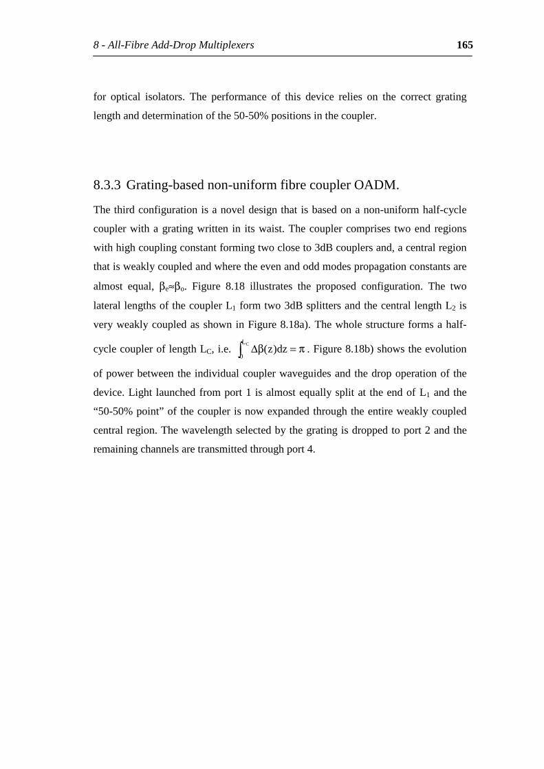
8-All-FibreAdd-DropMultiplexers 165
for optical isolators. The performance of this device relies on the correct grating
lengthanddeterminationofthe50-50%positionsinthecoupler.
8.3.3 Grating-basednon-uniformfibrecouplerOADM.
Thethirdconfigurationisanoveldesignthatisbasedonanon-uniformhalf-cycle
couplerwithagratingwritten in itswaist.Thecouplercomprises twoendregions
withhighcouplingconstantformingtwocloseto3dBcouplersand,acentralregion
thatisweaklycoupledandwheretheevenandoddmodespropagationconstantsare
almost equal, βe≈βo. Figure 8.18 illustrates the proposed configuration. The two
laterallengthsofthecouplerL1formtwo3dBsplittersandthecentrallengthL2is
veryweaklycoupledasshowninFigure8.18a).Thewholestructureformsahalf-
cyclecoupleroflengthLC,i.e. π=β∆CL
0dz)z( .Figure8.18b)showstheevolution
ofpowerbetweentheindividualcouplerwaveguidesandthedropoperationof the
device.Light launchedfromport1isalmostequallysplitat theendofL1andthe
“50-50%point”ofthecouplerisnowexpandedthroughtheentireweaklycoupled
centralregion.Thewavelengthselectedbythegratingisdroppedtoport2andthe
remainingchannelsaretransmittedthroughport4.
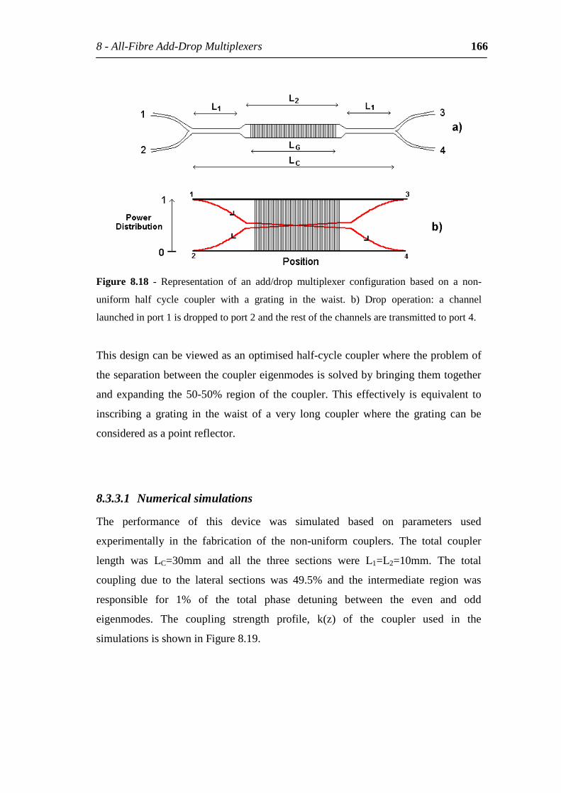
8-All-FibreAdd-DropMultiplexers 166
Figure 8.18 - Representation of an add/drop multiplexer configuration based on a non-
uniform half cycle coupler with a grating in the waist. b) Drop operation: a channel
launchedinport1isdroppedtoport2andtherestofthechannelsaretransmittedtoport4.
Thisdesigncanbeviewedasanoptimisedhalf-cyclecouplerwheretheproblemof
theseparationbetweenthecouplereigenmodesissolvedbybringingthemtogether
andexpanding the50-50% regionof the coupler.This effectively is equivalent to
inscribing a grating in the waist of a very long coupler where the grating can be
consideredasapointreflector.
8.3.3.1 Numericalsimulations
The performance of this device was simulated based on parameters used
experimentally in the fabrication of the non-uniform couplers. The total coupler
length was LC=30mm and all the three sections were L1=L2=10mm. The total
coupling due to the lateral sections was 49.5% and the intermediate region was
responsible for 1% of the total phase detuning between the even and odd
eigenmodes. The coupling strength profile, k(z) of the coupler used in the
simulationsisshowninFigure8.19.
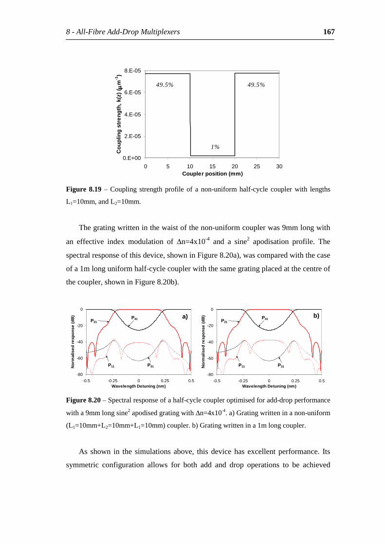
8-All-FibreAdd-DropMultiplexers 167
0.E+00
2.E-05
4.E-05
6.E-05
8.E-05
0 5 10 15 20 25 30Couplerposition(mm)
Cou
plin
gst
reng
th,k
(z)(
µµ µµm
-1)
49.5% 49.5%
1%
Figure8.19–Coupling strengthprofileof anon-uniformhalf-cycle couplerwith lengths
L1=10mm,andL2=10mm.
Thegratingwritteninthewaistofthenon-uniformcouplerwas9mmlongwith
an effective index modulation of ∆n=4x10⁻⁴ and a sine2 apodisation profile. The
spectralresponseofthisdevice,showninFigure8.20a),wascomparedwiththecase
ofa1mlonguniformhalf-cyclecouplerwiththesamegratingplacedatthecentreof
thecoupler,showninFigure8.20b).
-80
-60
-40
-20
0
-0.5 -0.25 0 0.25 0.5WavelengthDetuning(nm)
Nor
mal
ised
res
pons
e(d
B)
P11
P21P41
P31
a)
-80
-60
-40
-20
0
-0.5 -0.25 0 0.25 0.5WavelengthDetuning(nm)
Nor
mal
ised
res
pons
e(d
B)
P11
P21P41
P31
b)
Figure8.20–Spectralresponseofahalf-cyclecoupleroptimisedforadd-dropperformance
witha9mmlongsine2apodisedgratingwith∆n=4x10-4.a)Gratingwritteninanon-uniform
(L1=10mm+L2=10mm+L1=10mm)coupler.b)Gratingwrittenina1mlongcoupler.
As shown in the simulations above, thisdevice has excellentperformance. Its
symmetric configuration allows for both add and drop operations to be achieved
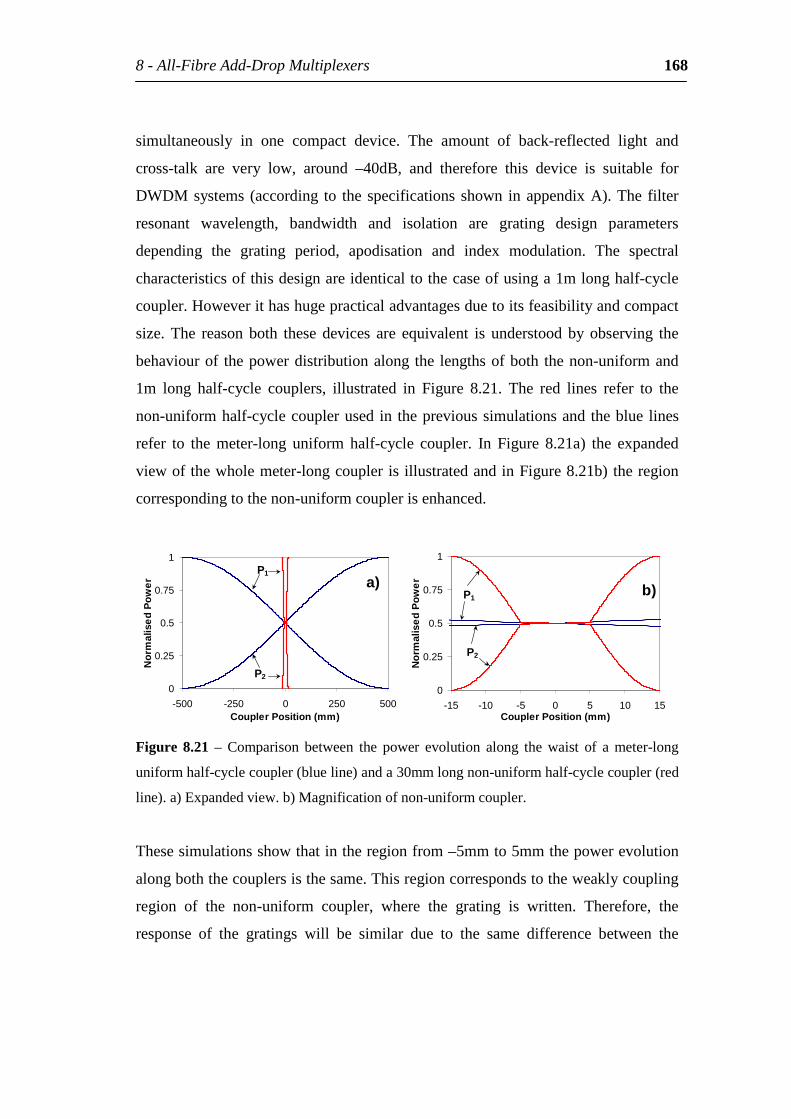
8-All-FibreAdd-DropMultiplexers 168
simultaneously in one compact device. The amount of back-reflected light and
cross-talk are very low, around –40dB, and therefore this device is suitable for
DWDMsystems (according to the specifications shown inappendixA).The filter
resonant wavelength, bandwidth and isolation are grating design parameters
depending the grating period, apodisation and index modulation. The spectral
characteristicsofthisdesignareidenticaltothecaseofusinga1mlonghalf-cycle
coupler.Howeverithashugepracticaladvantagesduetoitsfeasibilityandcompact
size. The reason both these devices are equivalent is understood by observing the
behaviourof thepowerdistributionalong the lengthsofboth thenon-uniformand
1m long half-cycle couplers, illustrated in Figure 8.21. The red lines refer to the
non-uniformhalf-cyclecouplerused in theprevioussimulationsand theblue lines
refer to the meter-long uniform half-cycle coupler. In Figure 8.21a) the expanded
viewofthewholemeter-longcouplerisillustratedandinFigure8.21b)theregion
correspondingtothenon-uniformcouplerisenhanced.
0
0.25
0.5
0.75
1
-500 -250 0 250 500CouplerPosition(mm)
Nor
mal
ised
Pow
er
P2
P1
a)
0
0.25
0.5
0.75
1
-15 -10 -5 0 5 10 15CouplerPosition(mm)
Nor
mal
ised
Pow
er
P2
P1b)
Figure 8.21 – Comparison between the power evolution along the waist of a meter-long
uniformhalf-cyclecoupler(blueline)anda30mmlongnon-uniformhalf-cyclecoupler(red
line).a)Expandedview.b)Magnificationofnon-uniformcoupler.
Thesesimulationsshowthatintheregionfrom–5mmto5mmthepowerevolution
alongboththecouplersisthesame.Thisregioncorrespondstotheweaklycoupling
region of the non-uniform coupler, where the grating is written. Therefore, the
response of the gratings will be similar due to the same difference between the
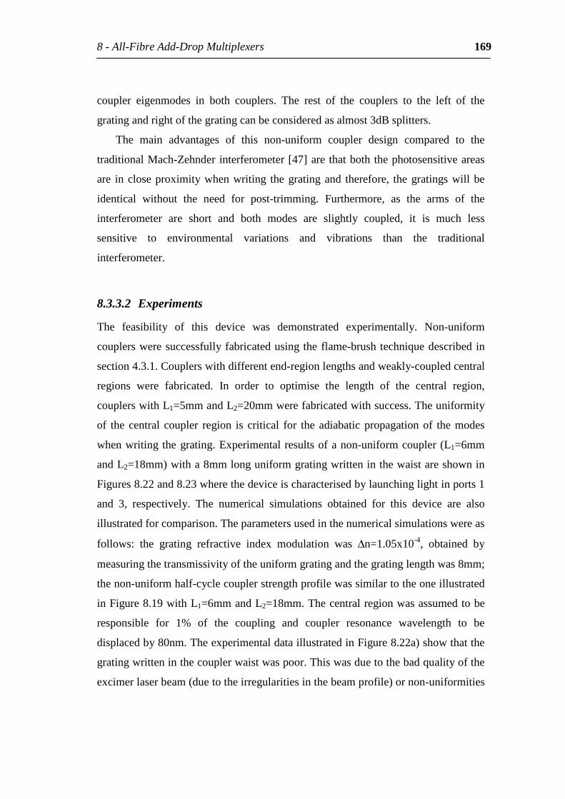
8-All-FibreAdd-DropMultiplexers 169
coupler eigenmodes in both couplers. The rest of the couplers to the left of the
gratingandrightofthegratingcanbeconsideredasalmost3dBsplitters.
The main advantages of this non-uniform coupler design compared to the
traditionalMach-Zehnderinterferometer[47]arethatboththephotosensitiveareas
are incloseproximitywhenwriting thegrating and therefore, thegratingswillbe
identical without the need for post-trimming. Furthermore, as the arms of the
interferometer are short and both modes are slightly coupled, it is much less
sensitive to environmental variations and vibrations than the traditional
interferometer.
8.3.3.2 Experiments
The feasibility of this device was demonstrated experimentally. Non-uniform
couplersweresuccessfullyfabricatedusingtheflame-brushtechniquedescribedin
section4.3.1.Couplerswithdifferentend-regionlengthsandweakly-coupledcentral
regions were fabricated. In order to optimise the length of the central region,
couplerswithL1=5mmandL2=20mmwerefabricatedwithsuccess.Theuniformity
of the central coupler region is critical for the adiabaticpropagationof themodes
whenwritingthegrating.Experimentalresultsofanon-uniformcoupler(L1=6mm
andL2=18mm)witha8mmlonguniformgratingwritteninthewaistareshownin
Figures8.22and8.23wherethedeviceischaracterisedbylaunchinglightinports1
and 3, respectively. The numerical simulations obtained for this device are also
illustratedforcomparison.Theparametersusedinthenumericalsimulationswereas
follows: the grating refractive index modulation was ∆n=1.05x10⁻⁴, obtained by
measuringthetransmissivityoftheuniformgratingandthegratinglengthwas8mm;
thenon-uniformhalf-cyclecouplerstrengthprofilewassimilartotheoneillustrated
inFigure8.19withL1=6mmandL2=18mm.Thecentralregionwasassumedtobe
responsible for 1% of the coupling and coupler resonance wavelength to be
displacedby80nm.TheexperimentaldataillustratedinFigure8.22a)showthatthe
gratingwritteninthecouplerwaistwaspoor.Thiswasduetothebadqualityofthe
excimerlaserbeam(duetotheirregularitiesinthebeamprofile)ornon-uniformities
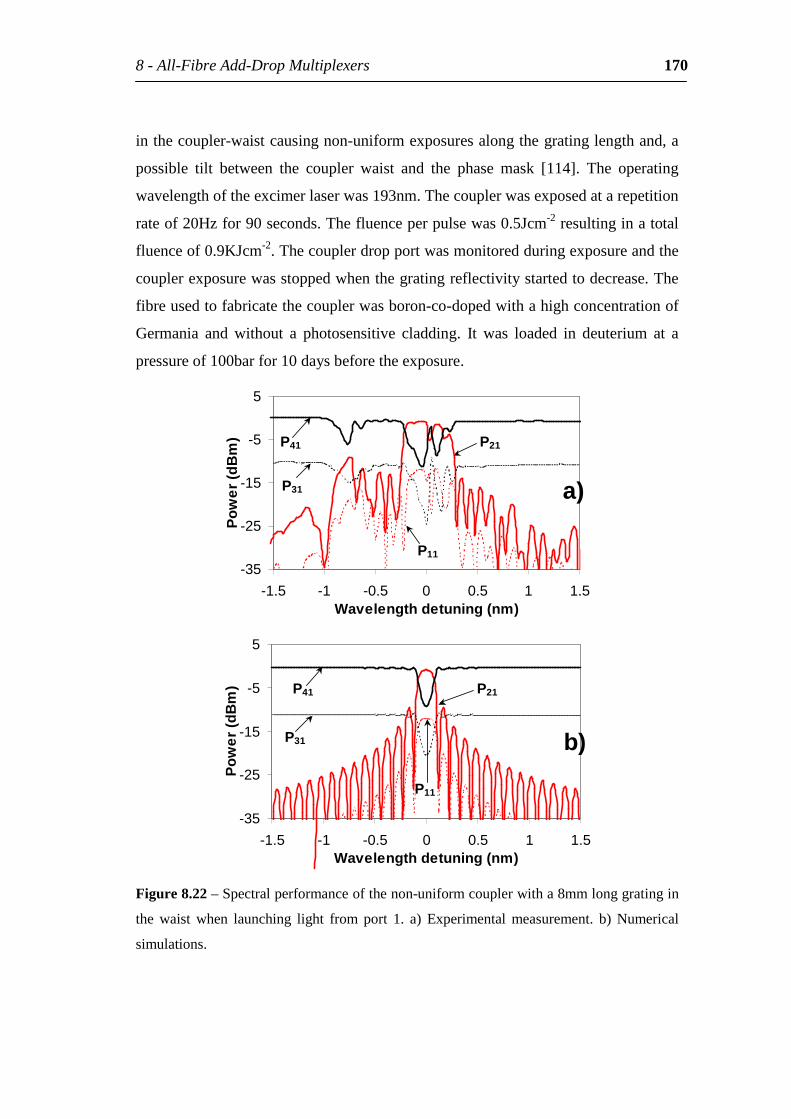
8-All-FibreAdd-DropMultiplexers 170
inthecoupler-waistcausingnon-uniformexposuresalongthegratinglengthand,a
possible tilt between the coupler waist and the phase mask [114]. The operating
wavelengthoftheexcimerlaserwas193nm.Thecouplerwasexposedatarepetition
rateof20Hzfor90seconds.Thefluenceperpulsewas0.5Jcm-2resultinginatotal
fluenceof0.9KJcm-2.Thecouplerdropportwasmonitoredduringexposureandthe
couplerexposurewasstoppedwhenthegratingreflectivitystartedtodecrease.The
fibreusedtofabricatethecouplerwasboron-co-dopedwithahighconcentrationof
Germania and without a photosensitive cladding. It was loaded in deuterium at a
pressureof100barfor10daysbeforetheexposure.
-35
-25
-15
-5
5
-1.5 -1 -0.5 0 0.5 1 1.5Wavelengthdetuning(nm)
Pow
er(d
Bm
)
P11
P31
P41 P21
a)
-35
-25
-15
-5
5
-1.5 -1 -0.5 0 0.5 1 1.5Wavelengthdetuning(nm)
Pow
er(d
Bm
)
P11
P31
P41 P21
b)
Figure8.22–Spectralperformanceofthenon-uniformcouplerwitha8mmlonggratingin
the waist when launching light from port 1. a) Experimental measurement. b) Numerical
simulations.
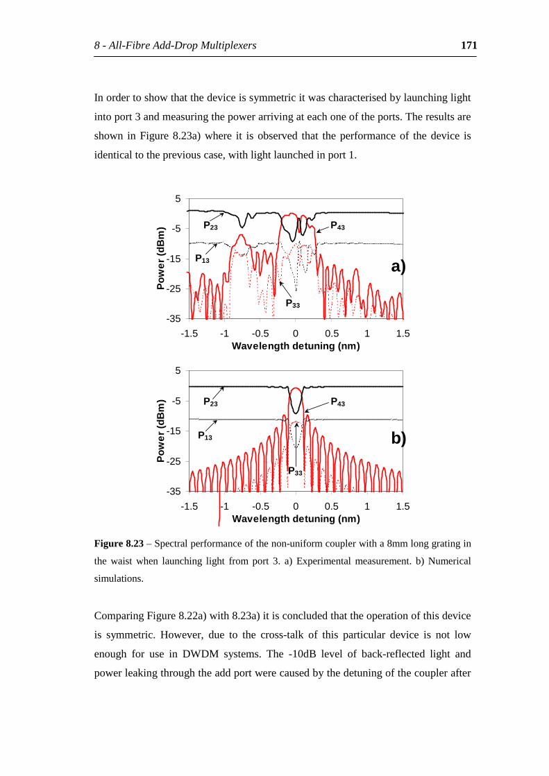
8-All-FibreAdd-DropMultiplexers 171
Inordertoshowthatthedeviceissymmetricitwascharacterisedbylaunchinglight
intoport3andmeasuringthepowerarrivingateachoneoftheports.Theresultsare
shown inFigure8.23a) where it is observed that theperformanceof thedevice is
identicaltothepreviouscase,withlightlaunchedinport1.
-35
-25
-15
-5
5
-1.5 -1 -0.5 0 0.5 1 1.5Wavelengthdetuning(nm)
Pow
er(d
Bm
)
P33
P13
P23 P43
a)
-35
-25
-15
-5
5
-1.5 -1 -0.5 0 0.5 1 1.5Wavelengthdetuning(nm)
Pow
er(d
Bm
)
P33
P13
P23 P43
b)
Figure8.23–Spectralperformanceofthenon-uniformcouplerwitha8mmlonggratingin
the waist when launching light from port 3. a) Experimental measurement. b) Numerical
simulations.
ComparingFigure8.22a)with8.23a)itisconcludedthattheoperationofthisdevice
is symmetric. However, due to the cross-talk of this particular device is not low
enough for use in DWDM systems. The -10dB level of back-reflected light and
powerleakingthroughtheaddportwerecausedbythedetuningofthecouplerafter
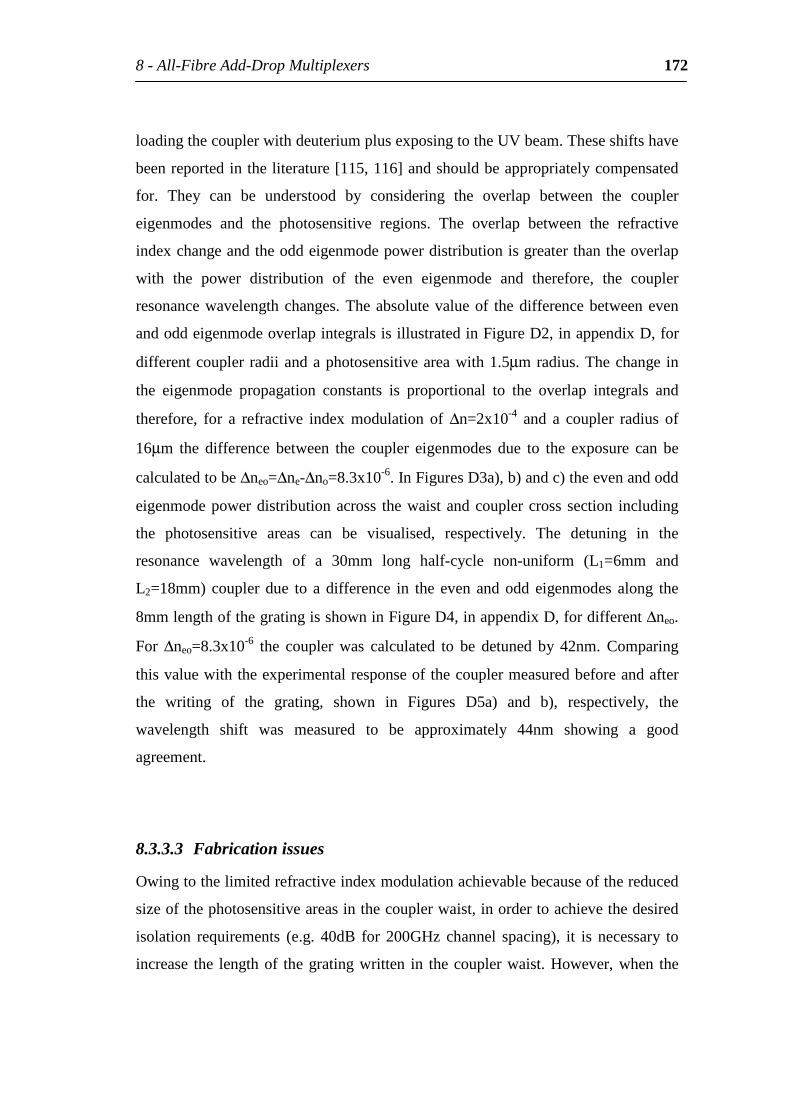
8-All-FibreAdd-DropMultiplexers 172
loadingthecouplerwithdeuteriumplusexposingtotheUVbeam.Theseshiftshave
beenreportedintheliterature[115,116]andshouldbeappropriatelycompensated
for. They can be understood by considering the overlap between the coupler
eigenmodes and the photosensitive regions. The overlap between the refractive
indexchangeandtheoddeigenmodepowerdistributionisgreaterthantheoverlap
with the power distribution of the even eigenmode and therefore, the coupler
resonancewavelengthchanges.Theabsolutevalueof thedifferencebetweeneven
andoddeigenmodeoverlapintegralsisillustratedinFigureD2,inappendixD,for
differentcoupler radiiandaphotosensitiveareawith1.5µmradius.Thechange in
the eigenmode propagation constants is proportional to the overlap integrals and
therefore, for a refractive index modulation of ∆n=2x10⁻⁴ and a coupler radius of
16µm the difference between the coupler eigenmodes due to the exposure can be
calculatedtobe∆neo=∆ne-∆no=8.3x10⁻⁶.InFiguresD3a),b)andc)theevenandodd
eigenmodepowerdistributionacross thewaistandcouplercross section including
the photosensitive areas can be visualised, respectively. The detuning in the
resonance wavelength of a 30mm long half-cycle non-uniform (L1=6mm and
L2=18mm)couplerdue to adifference in the evenandoddeigenmodes along the
8mmlengthofthegratingisshowninFigureD4,inappendixD,fordifferent∆neo.
For ∆neo=8.3x10⁻⁶ the coupler was calculated to be detuned by 42nm. Comparing
thisvaluewiththeexperimentalresponseofthecouplermeasuredbeforeandafter
the writing of the grating, shown in Figures D5a) and b), respectively, the
wavelength shift was measured to be approximately 44nm showing a good
agreement.
8.3.3.3 Fabricationissues
Owingtothelimitedrefractiveindexmodulationachievablebecauseofthereduced
sizeofthephotosensitiveareasinthecouplerwaist,inordertoachievethedesired
isolation requirements (e.g. 40dB for 200GHz channel spacing), it is necessary to
increase the lengthof thegratingwritten in thecouplerwaist.However,when the
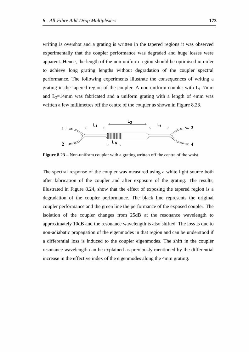
8-All-FibreAdd-DropMultiplexers 173
writing isovershot and agrating iswritten in the tapered regions itwasobserved
experimentally that the coupler performance was degraded and huge losses were
apparent.Hence,thelengthofthenon-uniformregionshouldbeoptimisedinorder
to achieve long grating lengths without degradation of the coupler spectral
performance. The following experiments illustrate the consequences of writing a
grating in the tapered regionof thecoupler.Anon-uniformcouplerwithL1=7mm
and L2=14mm was fabricated and a uniform grating with a length of 4mm was
writtenafewmillimetresoffthecentreofthecouplerasshowninFigure8.23.
Figure8.23–Non-uniformcouplerwithagratingwrittenoffthecentreofthewaist.
Thespectralresponseof thecouplerwasmeasuredusingawhite lightsourceboth
after fabrication of the coupler and after exposure of the grating. The results,
illustrated inFigure8.24, show that the effect of exposing the tapered region is a
degradation of the coupler performance. The black line represents the original
couplerperformanceandthegreenlinetheperformanceoftheexposedcoupler.The
isolation of the coupler changes from 25dB at the resonance wavelength to
approximately10dBandtheresonancewavelengthisalsoshifted.Thelossisdueto
non-adiabaticpropagationoftheeigenmodesinthatregionandcanbeunderstoodif
a differential loss is induced to the coupler eigenmodes. The shift in the coupler
resonancewavelengthcanbeexplainedaspreviouslymentionedbythedifferential
increaseintheeffectiveindexoftheeigenmodesalongthe4mmgrating.
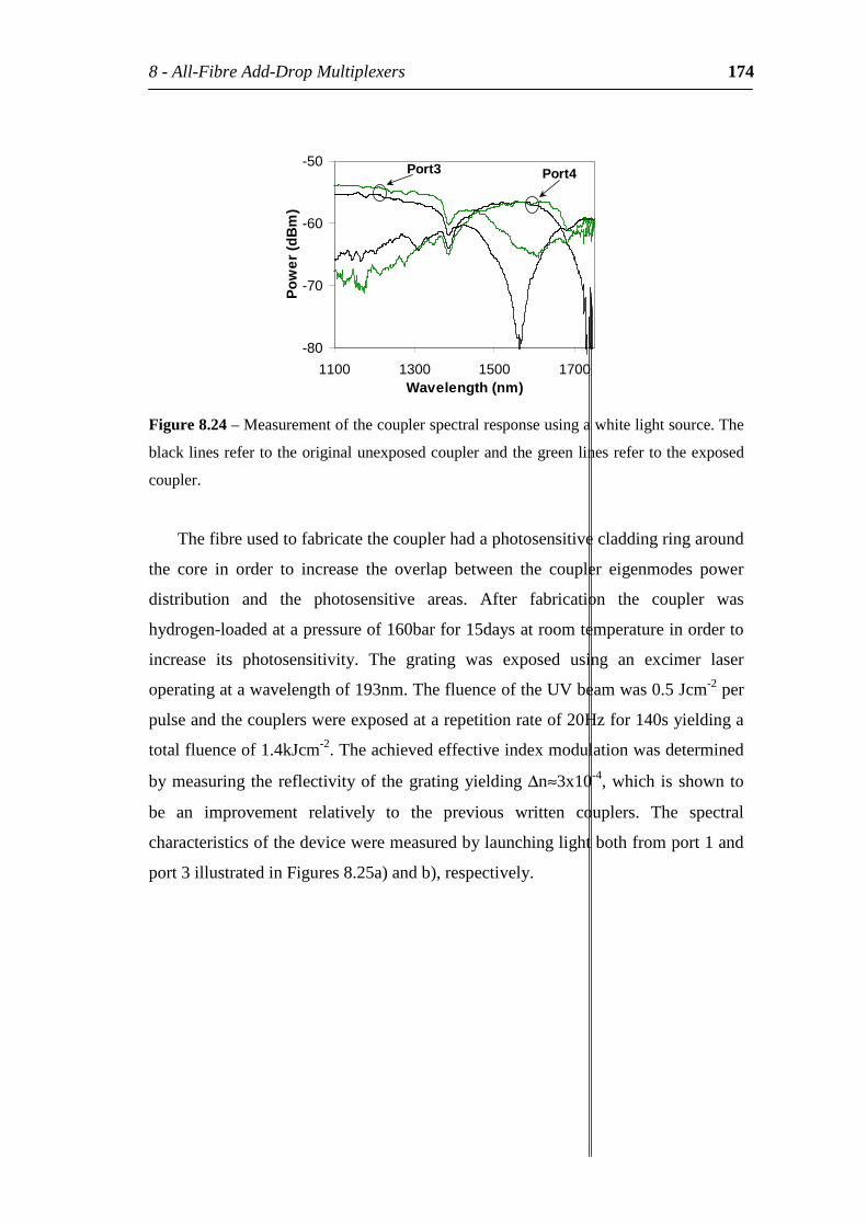
8-All-FibreAdd-DropMultiplexers 174
-80
-70
-60
-50
1100 1300 1500 1700Wavelength(nm)
Pow
er(d
Bm
)
Port3 Port4
Figure8.24–Measurementofthecouplerspectralresponseusingawhitelightsource.The
blacklinesrefertotheoriginalunexposedcouplerandthegreenlinesrefertotheexposed
coupler.
Thefibreusedtofabricatethecouplerhadaphotosensitivecladdingringaround
the core in order to increase the overlap between the coupler eigenmodes power
distribution and the photosensitive areas. After fabrication the coupler was
hydrogen-loadedatapressureof160barfor15daysatroomtemperatureinorderto
increase its photosensitivity. The grating was exposed using an excimer laser
operatingatawavelengthof193nm.ThefluenceoftheUVbeamwas0.5Jcm-2per
pulseandthecouplerswereexposedatarepetitionrateof20Hzfor140syieldinga
totalfluenceof1.4kJcm-2.Theachievedeffectiveindexmodulationwasdetermined
bymeasuringthereflectivityof thegratingyielding∆n≈3x10⁻⁴,whichisshownto
be an improvement relatively to the previous written couplers. The spectral
characteristicsofthedeviceweremeasuredbylaunchinglightbothfromport1and
port3illustratedinFigures8.25a)andb),respectively.
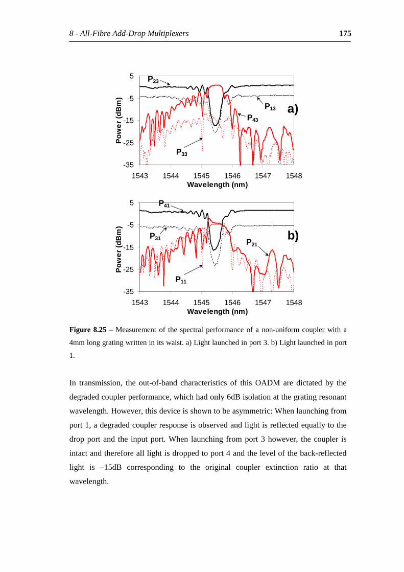
8-All-FibreAdd-DropMultiplexers 175
-35
-25
-15
-5
5
1543 1544 1545 1546 1547 1548Wavelength(nm)
Pow
er(d
Bm
)
P33
P23
P13
P43
a)
-35
-25
-15
-5
5
1543 1544 1545 1546 1547 1548Wavelength(nm)
Pow
er(d
Bm
)
P11
P31
P41
P21b)
Figure8.25–Measurementof the spectralperformanceofanon-uniformcouplerwitha
4mmlonggratingwritteninitswaist.a)Lightlaunchedinport3.b)Lightlaunchedinport
1.
In transmission, the out-of-band characteristics of this OADM are dictated by the
degradedcouplerperformance,whichhadonly6dBisolationatthegratingresonant
wavelength.However,thisdeviceisshowntobeasymmetric:Whenlaunchingfrom
port1,adegradedcouplerresponseisobservedandlightisreflectedequallytothe
dropportand the inputport.When launching fromport3however, the coupler is
intactandthereforealllightisdroppedtoport4andtheleveloftheback-reflected
light is –15dB corresponding to the original coupler extinction ratio at that
wavelength.
8-All-FibreAdd-DropMultiplexers 176
8.3.3.4 Conclusions
An improved add-drop performance can be achieved by using a complex coupler
design that is based on a non-uniform coupler. Theoretically this device is
equivalent to a uniform half-cycle configuration with a very long coupler length
yieldingoptimumcross-talkcharacteristics.However,as inall thesecoupler-based
devices, efforts shouldbemade to increase the grating strengthby increasing: the
fibre photosensitivity; the overlap between the photosensitive areas and the field
distributionofthecouplereigenmodes;andthelengthofthenon-uniformregionof
the coupler. A refractive index modulation of ∆n=3x10⁻⁴ that could yield an
extinction ratio of –29dB using a 16mm long grating with sine2 apodisation was
experimentallyachieved.Thecorrectpositionof thegratinginthecouplerwaistis
criticalfortheoperationofthedevicedependingontheexactdeterminationofthe
uniform region in the centre of the coupler. The method for characterising fibre
couplers developed in Chapter 9 is suitable for the experimental determination of
theseregions.
8.4 Summary
Limitationsandoptimisationofdifferentadd-dropmultiplexerconfigurationswere
discussed.Firstly,aconfigurationusingauniformhalf-cyclecouplerwithagrating
inscribedinthewaistwasanalysed.Itcanbeoptimisedbycascadingtwoidentical
asymmetricdeviceswherethegratingisdisplacedfromthecentreofthecoupleror,
by fabricating extremely long couplers where the grating can be considered as a
pointreflector.However, thegratingstrength,apodisationandidentificationof the
position within the coupler, where it should be placed and the difficulty of
fabricating long uniform couplers are serious problems that compromise its
performance.Additionally,theirreducedphotosensitivityandtheconsequentlimited
channelisolationofthegratingfiltersisanotherlimitationthathastobeovercome.
Todetermineexperimentallythepositionofthecentreofthehalf-cyclecoupleror,
8-All-FibreAdd-DropMultiplexers 177
optimise their fabrication procedure, a non-destructive method for characterising
fibrecouplerswasdevelopedandisdiscussedinChapter9.
Secondly,aconfigurationbasedonafull-cyclecouplerwithagratinginscribed
initswaist,placedbetweenitstwo50-50%points,wasstudied.Thisdevicesuffers
fromintrinsichighout-of-bandback-reflectionsandcross-talkwhenitsisolationis
optimised. However, the device isolation of the grating channel depends on the
usingtheexactgratinglengthbydeterminingthepositionof the50-50%pointsof
the coupler. These can again be experimentally determined by the coupler
characterisationmethoddevelopedinthefollowingchapter.
Finally, a device based on a non-uniform half-cycle coupler that theoretically
yields an optimum add-drop multiplexer performance was demonstrated to be
suitableforDWDM.ItissymmetricachievingbothAddandDropfunctionsinone
compact device. The grating, written in the slightly-coupled central region, is
position independent as longas the tapered regions arenot exposed.Asymmetric
devicewasexperimentallydemonstratedsuggestingthatthetwoendregionsofthe
couplerwerewellmatched.Maindrawbacksforthisdeviceisthelimitedsizeofthe
central regionhence thegrating length.Procedures for fabricating longer couplers
with a better control over the central region shape, length should be investigated.
The accurate placement of the grating within the coupler can be achieved by
characterisingitusingthemethodexploitedinChapter9.
9
CharacterisationofFibre-
Couplers
Anovelnon-destructive technique for characterising couplersbymeans of a local
perturbation is described. The method is studied theoretically and verified
experimentallybycharacterisingdifferent typesof fused fibre-couplers.Using this
technique,boththeinformationofthepowerdistributionandcouplingprofilealong
thecouplerwaistareobtained.
9-CharacterisationofFibre-Couplers 179
9.1 Introduction
The performance of couplers and coupler-based devices depends on the coupling-
constant and/or power distribution along the coupling region. The response of
coupler-based OADMs involving Bragg gratings, for example, is critically
dependentontheexactpositioningofthegratingwithrespecttothepointsinsidethe
couplerwaistwherethepoweroneachindividualcoreisequallysplitasmentioned
in chapter 8, or equivalently, where the phase difference between the two waist
eigenmodes is multiple of π/2. Development of non-destructive coupler
characterisationtechniques,inordertodeterminethepowerevolutionandcoupling
constant distribution along the coupler length, is, therefore, of paramount
importanceindevelopingcouplersforhighperformanceapplications.
Various methods for determining different parameters of uniform directional
couplershavebeenreportedintheliterature[117,118].Bourbinetal.[118]reported
amethodforcharacterisingcouplersinplanarwaveguides.Themethodisbasedon
inducing a small differential loss in one of the coupled waveguides. In order to
localisethelossperturbationinoneofthewaveguidesonly,theotherwaveguideis
covered with aprotective resist film.Gnewuchet al. [117] reported an alternative
local-perturbation method for measuring the beatlength of uniform couplers in
buried planar-waveguide geometry. The method consists of inducing a local
perturbation in one of the waveguides by heating it with an incident 980 nm
semiconductor laser diode. To facilitate the 980 nm laser absorption by the
otherwise transparent waveguides and achieve local heating, a 1µm-thick layer of
absorptiveblackinkwasspin-coatedontothecouplersurface.Themethoddidnot
giveanyresultswhenthecouplerwasperturbedsymmetrically(laserdiodefocused
at the centre between the two waveguides). It should be stressed that the two
reported methods require some degree of post-fabrication coupler treatment (e.g.,
applicationofresistfilminoneofthewaveguides[118]andspin-coatedabsorptive
thin-layer[117])inordertoachievetherequireddifferentialperturbation.Although
such steps and processes can be acceptable in planar waveguide geometries, they
cannot be applied or should be avoided in fused fibre coupler geometries. This is
9-CharacterisationofFibre-Couplers 180
due to the fact that the very small waist diameters involved are quite fragile and
pronetopost-fabrication-treatmentfailures.
Inthischapter,anewnon-destructivemethodforfullcouplercharacterisationis
described.Themethoddoesnotinvolveanypost-fabricationtreatmentand/orextra
coupler preparation. Firstly, by applying an asymmetric perturbation between the
two lowest-orderwaist eigenmodes, the complexpower evolution along the entire
coupling region can be measured non-destructively. Furthermore, in the particular
case of a 100% coupler, the asymmetric perturbation of the coupler provides a
markerforthepositionalongthecouplerwherethepowerisequallysplitbetween
both the waveguides (50-50% point) independently of the wavelength of the light
used to monitor the coupler. Secondly, by applying a symmetric perturbation
between the two lowest-orderwaisteigenmodes, thecoupling-constantdistribution
alongtheentirecouplingregioncanbemeasuredwithoutdamagingthecoupler.
9.2 Local Perturbation Coupler Characterisation
Technique
9.2.1 GeneralDescriptionoftheProposedMethod
As already mentioned, optical couplers are formed by bringing two or more
waveguides(planar,ridge,diffusedwaveguidesorfibres)incloseproximitysothat
they exchange power through evanescent field interaction. In four-port (2x2)
couplers,shownschematicallyinFigure4.1,twowaveguidesexchangepowersover
acoupling region (LC),whichcomprises thecouplerwaist (LW)and the two taper
regions (LT1,LT2)on either side.The taper regionsareadiabatic inorder toavoid
higher-order, as well as, radiation mode excitation that contribute to losses. The
coupling process along the taper lengths is non-uniform, described by a varying
couplingconstant,andaccountsforasubstantialpartofthetotalexchangedpower.
These regions should be taken into account when considering practical coupled
9-CharacterisationofFibre-Couplers 181
devices.Thewaistregion,ontheotherhand,inmostofthecasesissupposedtobe
uniform and is described by a fixed coupling constant. However, in practise,
dependingonthefabricationprocess,thewaistshowssizeablenon-uniformitiesthat
should be properly accounted for, in order to describe accurately the device
performance. This is particularly important in more complex devices, such as
OADMs,thatcombinecouplerswithgratingsintheirwaistsasdiscussedinchapter
8.
Figure 9.1a) illustrates the principle of operation of the proposed technique.
Lightof theappropriatewavelength is launched intooneof the inputports (#1or
#2). The coupler characterisation method consists of inducing a local perturbation
along its coupling region (taper + waist) and monitoring the change in power (or
phase) at oneor twoof theoutputports (#3 and#4).The localperturbation is, in
general, induced non-destructively by a temperature gradient across the coupler
waist,asshownschematicallyinFigure9.1.Theperturbation(shownbytheshaded
area)canbeasymmetric(Figure9.1b)-top)orsymmetric(Figure9.1b)-bottom)with
respecttothepowerdistributionofevenandoddeigenmodes.Asitwillbeshown
theoretically and confirmed experimentally in subsequent sections, the type of the
applied perturbation can provide information about different coupler parameters.
The temperature gradients were induced by two different techniques, involving
differentheatsources.Thefirstonewasaheatedwireandthesecondoneapower-
controlled CO2 laser. The CO2 laser radiation is highly absorbed by fused silica
(typical absorption length of ~5µm [119]) and provides the required perturbation
gradientwithouttheneedforapplicationofextraabsorbinglayers(asinRef.[117]).
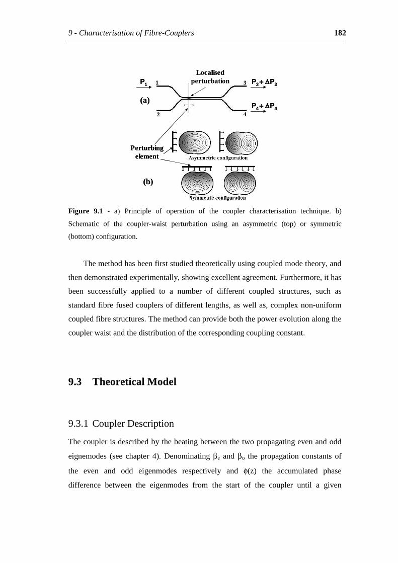
9-CharacterisationofFibre-Couplers 182
Perturbingelement
P1
P4++++ ∆∆∆∆P4
P3++++ ∆∆∆∆P3
Localisedperturbation
(b)
(a)
Perturbingelement
P1
P4++++ ∆∆∆∆P4
P3++++ ∆∆∆∆P3
Localisedperturbation
(b)
(a)
Figure 9.1 - a) Principle of operation of the coupler characterisation technique. b)
Schematic of the coupler-waist perturbation using an asymmetric (top) or symmetric
(bottom)configuration.
Themethodhasbeenfirststudiedtheoreticallyusingcoupledmodetheory,and
thendemonstratedexperimentally,showingexcellentagreement.Furthermore,ithas
been successfully applied to a number of different coupled structures, such as
standardfibrefusedcouplersofdifferentlengths,aswellas,complexnon-uniform
coupledfibrestructures.Themethodcanprovideboththepowerevolutionalongthe
couplerwaistandthedistributionofthecorrespondingcouplingconstant.
9.3 TheoreticalModel
9.3.1 CouplerDescription
Thecouplerisdescribedbythebeatingbetweenthetwopropagatingevenandodd
eignemodes (see chapter 4). Denominating βe andβo the propagation constants of
the even and odd eigenmodes respectively and φ(z) the accumulated phase
difference between the eigenmodes from the start of the coupler until a given
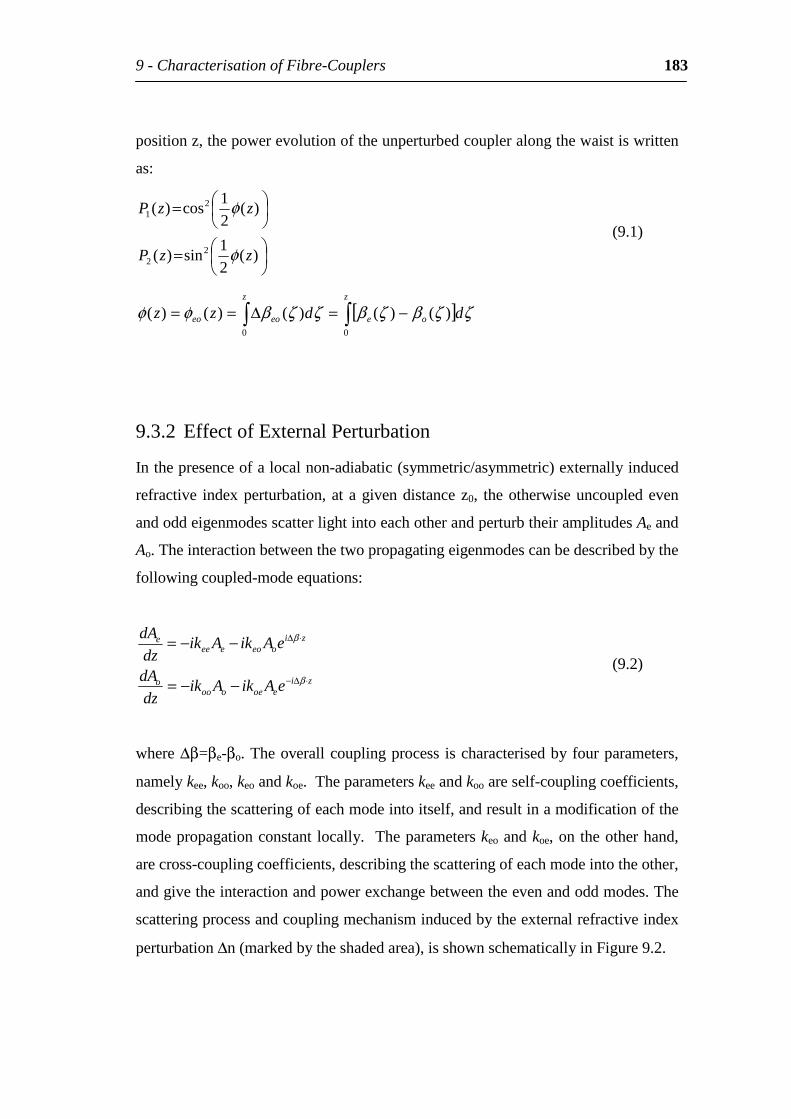
9-CharacterisationofFibre-Couplers 183
positionz,thepowerevolutionoftheunperturbedcoupleralongthewaistiswritten
as:
=
=
)(21
sin)(
)(21
cos)(
22
21
zzP
zzP
φ
φ (9.1)
[ ] −=∆==z
oe
z
eoeo ddzz00
)()()()()( ζζβζβζζβφφ
9.3.2 EffectofExternalPerturbation
Inthepresenceofalocalnon-adiabatic(symmetric/asymmetric)externallyinduced
refractive indexperturbation,atagivendistancez0, theotherwiseuncoupledeven
andoddeigenmodesscatterlightintoeachotherandperturbtheiramplitudesAeand
Ao.Theinteractionbetweenthetwopropagatingeigenmodescanbedescribedbythe
followingcoupled-modeequations:
zieoeooo
o
zioeoeee
e
eAikAikdzdA
eAikAikdzdA
⋅∆−
⋅∆
−−=
−−=
β
β
(9.2)
where∆β=βe-βo.Theoverallcouplingprocess ischaracterisedby fourparameters,
namelykee,koo,keoandkoe.Theparameterskeeandkooareself-couplingcoefficients,
describingthescatteringofeachmodeintoitself,andresultinamodificationofthe
modepropagationconstant locally. Theparameterskeoandkoe,ontheotherhand,
arecross-couplingcoefficients,describingthescatteringofeachmodeintotheother,
andgivetheinteractionandpowerexchangebetweentheevenandoddmodes.The
scatteringprocessandcouplingmechanisminducedbytheexternalrefractiveindex
perturbation∆n(markedbytheshadedarea),isshownschematicallyinFigure9.2.
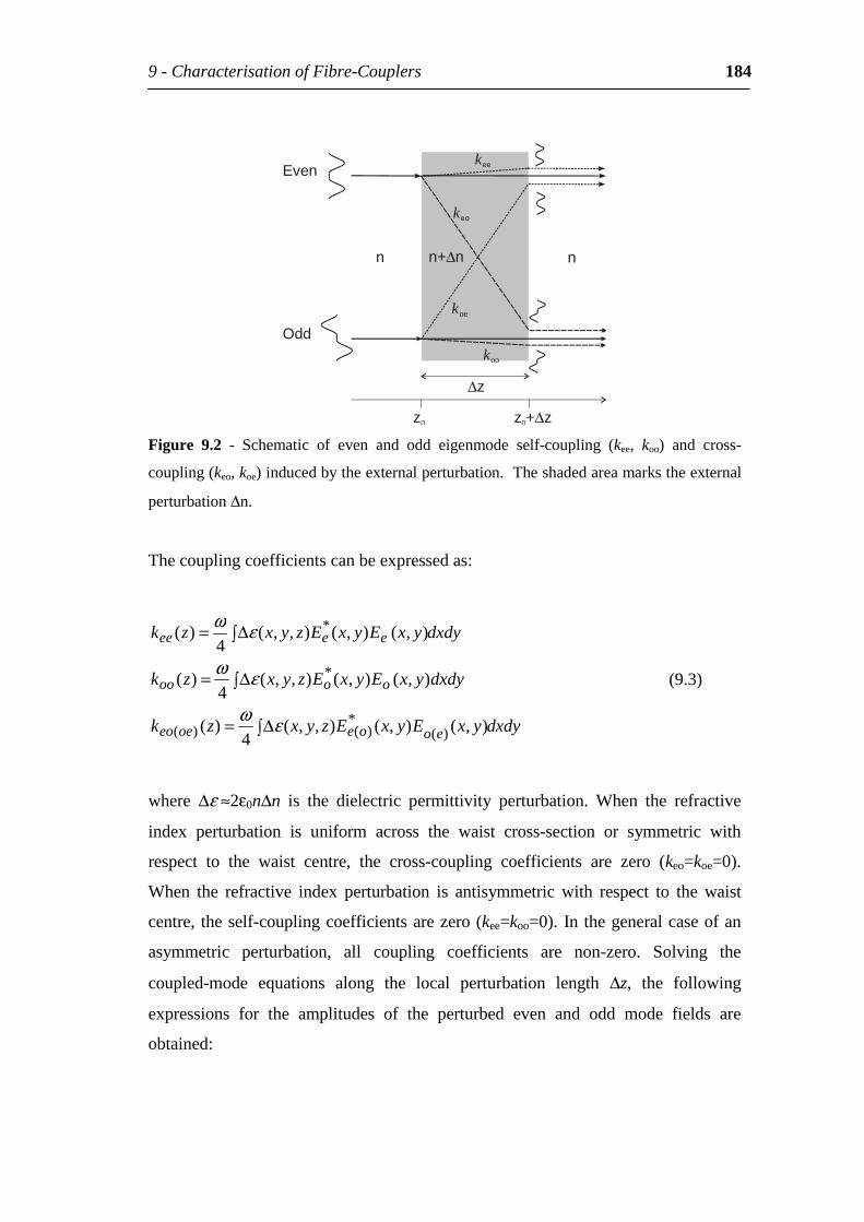
9-CharacterisationofFibre-Couplers 184
Evenkee
koo
keo
koe
Odd
z0
∆z
z + z0 ∆
n n+ n∆ n
Figure 9.2 - Schematic of even and odd eigenmode self-coupling (kee, koo) and cross-
coupling(keo,koe)inducedbytheexternalperturbation.Theshadedareamarkstheexternal
perturbation∆n.
Thecouplingcoefficientscanbeexpressedas:
dxdyyxEyxEzyxzk
dxdyyxEyxEzyxzk
dxdyyxEyxEzyxzk
eooeoeeo
oooo
eeee
∆=
∆=
∆=
),(),(),,(4
)(
),(),(),,(4
)(
),(),(),,(4
)(
)(*
)()(
*
*
εω
εω
εω
(9.3)
where ∆ε≈2ε0n∆n is the dielectric permittivity perturbation. When the refractive
index perturbation is uniform across the waist cross-section or symmetric with
respect to the waist centre, the cross-coupling coefficients are zero (keo=koe=0).
When the refractive index perturbation is antisymmetric with respect to the waist
centre, theself-couplingcoefficientsarezero(kee=koo=0). Inthegeneralcaseofan
asymmetric perturbation, all coupling coefficients are non-zero. Solving the
coupled-mode equations along the local perturbation length ∆z, the following
expressions for the amplitudes of the perturbed even and odd mode fields are
obtained:
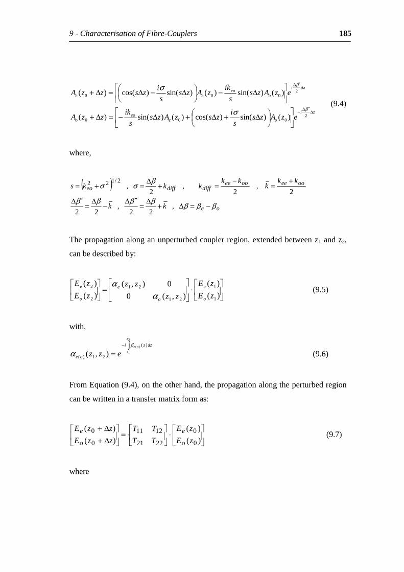
9-CharacterisationofFibre-Couplers 185
zi
oeeo
o
zi
oeo
ee
ezAzss
izszAzs
sik
zzA
ezAzss
ikzAzs
si
zszzA
∆′′∆−
∆′∆
∆+∆+∆−=∆+
∆−
∆−∆=∆+
2000
2000
)()sin()cos()()sin()(
)()sin()()sin()cos()(
β
β
σ
σ
(9.4)
where,
( )oe
ooeeooeediffdiffeo
kk
kkk
kkkkks
βββββββ
βσσ
−=∆+∆
=′′∆
−∆
=′∆
+=
−=+
∆=+=
,22
,22
2,
2,
2,
2/122
Thepropagationalonganunperturbedcouplerregion,extendedbetweenz1andz2,
canbedescribedby:
⋅
=
)()(
),(00),(
)()(
1
1
21
21
2
2
zE
zE
zz
zzzE
zE
o
e
o
e
o
e
αα
(9.5)
with,
=
−2
1
)( )(
21)( ),(
z
z
oe dzzi
oe ezzβ
α (9.6)
FromEquation(9.4),ontheotherhand,thepropagationalongtheperturbedregion
canbewritteninatransfermatrixformas:
⋅
⋅=
∆+∆+
)()(
)()(
0
0
2221
1211
0
0zE
zE
TT
TTzzE
zzE
o
e
o
e (9.7)
where
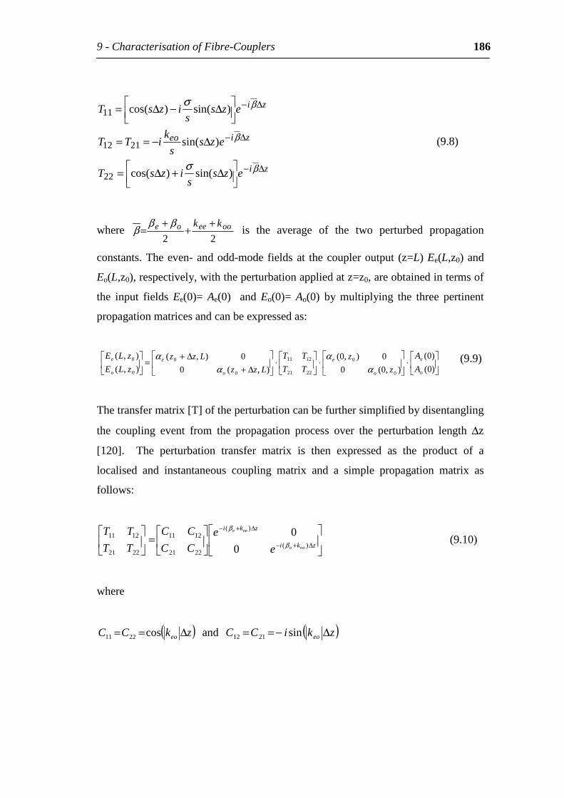
9-CharacterisationofFibre-Couplers 186
zi
zieo
zi
ezss
izsT
ezss
kiTT
ezss
izsT
∆−
∆−
∆−
∆+∆=
∆−==
∆−∆=
β
β
β
σ
σ
)sin()cos(
)sin(
)sin()cos(
22
2112
11
(9.8)
where22
ooeeoe kk ++
+=
βββ is the average of the two perturbed propagation
constants.Theeven-andodd-modefieldsat thecoupleroutput (z=L)Ee(L,z0)and
Eo(L,z0),respectively,withtheperturbationappliedatz=z0,areobtainedintermsof
the input fields Ee(0)= Ae(0) and Eo(0)= Ao(0) by multiplying the three pertinent
propagationmatricesandcanbeexpressedas:
⋅
⋅
⋅
∆+∆+
=
)0()0(
),0(00),0(
),(00),(
),(),(
0
0
2221
1211
0
0
0
0
o
e
o
e
o
e
o
e
A
A
zz
TT
TT
LzzLzz
zLE
zLE
αα
αα (9.9)
Thetransfermatrix[T]oftheperturbationcanbefurthersimplifiedbydisentangling
the coupling event from the propagation process over the perturbation length ∆z
[120]. The perturbation transfer matrix is then expressed as the product of a
localised and instantaneous coupling matrix and a simple propagation matrix as
follows:
=
∆+−
∆+−
zki
zki
ooo
eee
e
eCC
CC
TT
TT)(
)(
2221
1211
2221
1211
00
β
β
(9.10)
where
( )zkCC eo ∆== cos2211 and ( )zkiCC eo ∆−== sin2112
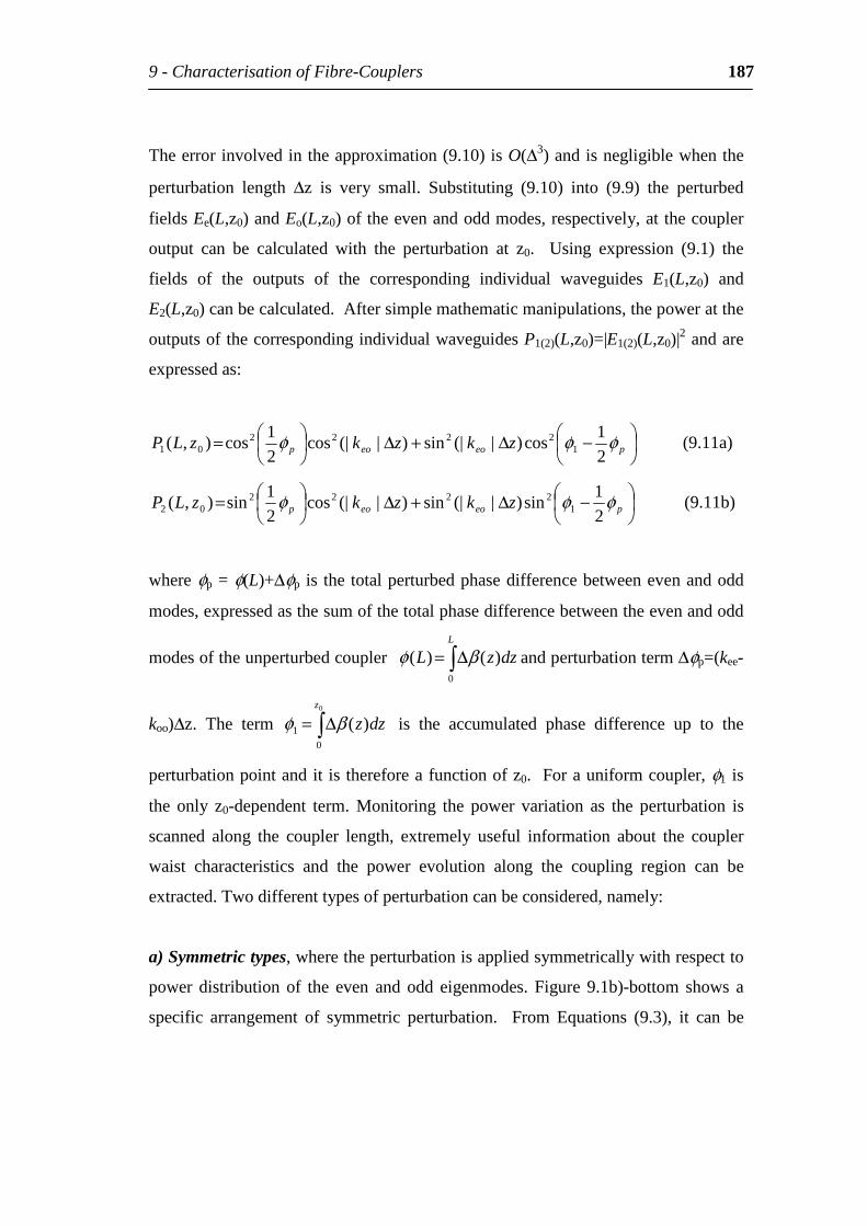
9-CharacterisationofFibre-Couplers 187
Theerrorinvolvedintheapproximation(9.10)isO(∆3)andisnegligiblewhenthe
perturbation length ∆z is very small. Substituting (9.10) into (9.9) the perturbed
fieldsEe(L,z0)andEo(L,z0)oftheevenandoddmodes,respectively,atthecoupler
output can be calculated with the perturbation at z0. Using expression (9.1) the
fields of the outputs of the corresponding individual waveguides E1(L,z0) and
E2(L,z0)canbecalculated.Aftersimplemathematicmanipulations,thepoweratthe
outputsofthecorrespondingindividualwaveguidesP1(2)(L,z0)=|E1(2)(L,z0)|2andare
expressedas:
−∆+∆
= peoeop zkzkzLP φφφ21
cos)|(|sin)|(|cos21
cos),( 12222
01 (9.11a)
−∆+∆
= peoeop zkzkzLP φφφ21
sin)|(|sin)|(|cos21
sin),( 12222
02 (9.11b)
whereφp=φ(L)+∆φp is thetotalperturbedphasedifferencebetweenevenandodd
modes,expressedasthesumofthetotalphasedifferencebetweentheevenandodd
modesoftheunperturbedcoupler ∆=L
dzzL0
)()( βφ andperturbationterm∆φp=(kee-
koo)∆z. The term ∆=0
01 )(
z
dzzβφ is the accumulated phase difference up to the
perturbationpointanditisthereforeafunctionofz0. Forauniformcoupler,φ1is
the only z0-dependent term. Monitoring the power variation as the perturbation is
scanned along the coupler length, extremely useful information about the coupler
waist characteristics and the power evolution along the coupling region can be
extracted.Twodifferenttypesofperturbationcanbeconsidered,namely:
a)Symmetrictypes,wheretheperturbationisappliedsymmetricallywithrespectto
power distribution of the even and odd eigenmodes. Figure 9.1b)-bottom shows a
specific arrangement of symmetric perturbation. From Equations (9.3), it can be
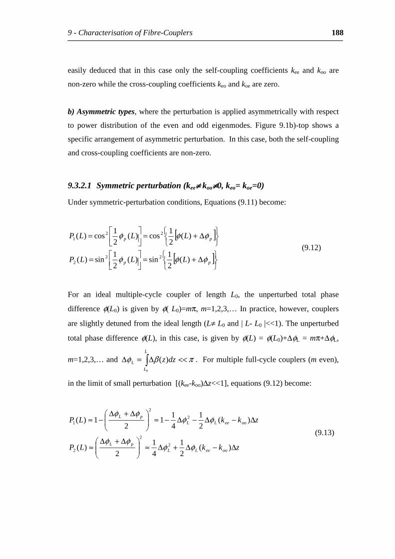
9-CharacterisationofFibre-Couplers 188
easily deduced that in this case only the self-coupling coefficients kee and koo are
non-zerowhilethecross-couplingcoefficientskeoandkoearezero.
b)Asymmetrictypes,wheretheperturbationisappliedasymmetricallywithrespect
to power distribution of the even and odd eigenmodes. Figure 9.1b)-top shows a
specificarrangementofasymmetricperturbation.Inthiscase,boththeself-coupling
andcross-couplingcoefficientsarenon-zero.
9.3.2.1 Symmetricperturbation(kee≠≠≠≠koo≠≠≠≠0,keo=koe=0)
Undersymmetric-perturbationconditions,Equations(9.11)become:
[ ]
[ ]
∆+=
=
∆+=
=
pp
pp
LLLP
LLLP
φφφ
φφφ
)(21
sin)(21
sin)(
)(21
cos)(21
cos)(
222
221
(9.12)
For an ideal multiple-cycle coupler of length L0, the unperturbed total phase
difference φ(L0) is givenby φ(L0)=mπ,m=1,2,3,… Inpractice,however, couplers
areslightlydetunedfromtheideallength(L≠L0and|L-L0|<<1).Theunperturbed
total phasedifference φ(L), in this case, is givenby φ(L)= φ(L0)+∆φL=mπ+∆φL,
m=1,2,3,… and πβφ <<∆=∆ L
LL dzz
0
)( .Formultiplefull-cyclecouplers(meven),
inthelimitofsmallperturbation[(kee-koo)∆z<<1],equations(9.12)become:
zkkLP
zkkLP
ooeeLLpL
ooeeLLpL
∆−∆+∆≈
∆+∆≈
∆−∆−∆−≈
∆+∆−≈
)(21
41
2)(
)(21
41
12
1)(
2
2
2
2
2
1
φφφφ
φφφφ
(9.13)
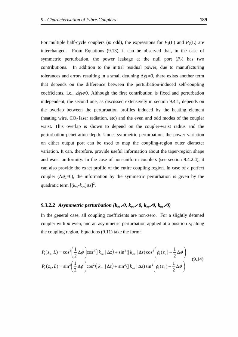
9-CharacterisationofFibre-Couplers 189
For multiple half-cycle couplers (m odd), the expressions for P1(L) and P2(L) are
interchanged. From Equations (9.13), it can be observed that, in the case of
symmetric perturbation, the power leakage at the null port (P2) has two
contributions. In addition to the initial residual power, due to manufacturing
tolerancesanderrorsresultinginasmalldetuning∆φL≠0,thereexistsanotherterm
that depends on the difference between the perturbation-induced self-coupling
coefficients, i.e., ∆φP≠0. Although the first contribution is fixed and perturbation
independent, thesecondone,asdiscussedextensively insection9.4.1,dependson
the overlap between the perturbation profiles induced by the heating element
(heatingwire,CO2laser radiation,etc)andtheevenandoddmodesof thecoupler
waist. This overlap is shown to depend on the coupler-waist radius and the
perturbation penetration depth. Under symmetric perturbation, the power variation
on either output port can be used to map the coupling-region outer diameter
variation.Itcan,therefore,provideusefulinformationaboutthetaper-regionshape
and waist uniformity. In the case of non-uniform couplers (see section 9.4.2.4), it
canalsoprovidetheexactprofileoftheentirecouplingregion.Incaseofaperfect
coupler (∆φL=0), the information by the symmetric perturbation is given by the
quadraticterm[(kee-koo)∆z]2.
9.3.2.2 Asymmetricperturbation(kee≠≠≠≠0,koo≠≠≠≠0,keo≠≠≠≠0,koe≠≠≠≠0)
In the general case, all coupling coefficients arenon-zero. For a slightly detuned
couplerwithmeven,andanasymmetricperturbationappliedatapositionz0along
thecouplingregion,Equations(9.11)taketheform:
( )
( )
∆−∆+∆
∆=
∆−∆+∆
∆=
φφφ
φφφ
21
)(sin)|(|sin||cos21
sin),(
21
)(cos)|(|sin||cos21
cos),(
012222
02
012222
01
zzkzkLzP
zzkzkLzP
eoeo
eoeo
(9.14)
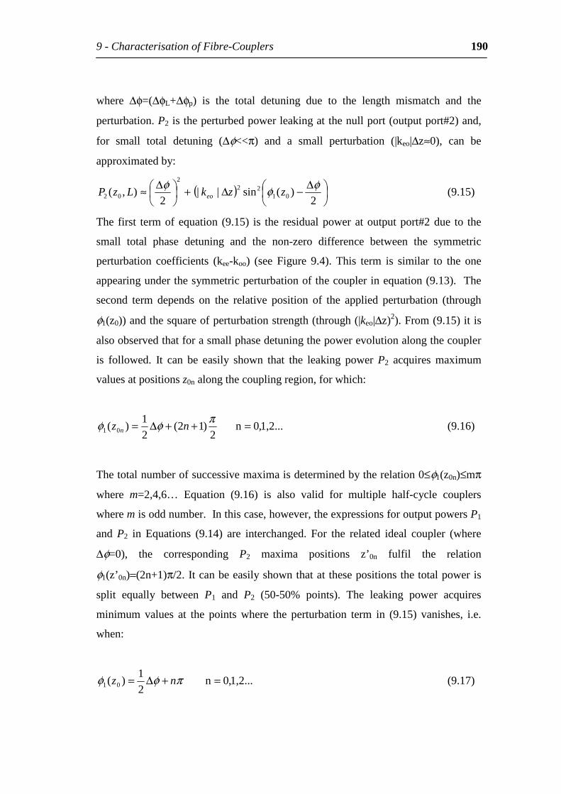
9-CharacterisationofFibre-Couplers 190
where ∆φ=(∆φL+∆φp) is the total detuning due to the length mismatch and the
perturbation.P2istheperturbedpowerleakingatthenullport(outputport#2)and,
for small total detuning (∆φ<<π) and a small perturbation (|keo|∆z≈0), can be
approximatedby:
( )
∆−∆+
∆≈2
)(sin||2
),( 0122
2
02φφφ
zzkLzP eo (9.15)
The first termof equation (9.15) is the residualpower atoutputport#2due to the
small total phase detuning and the non-zero difference between the symmetric
perturbation coefficients (kee-koo) (see Figure 9.4). This term is similar to the one
appearingunderthesymmetricperturbationofthecouplerinequation(9.13).The
second term depends on the relative position of the applied perturbation (through
φ1(z0))andthesquareofperturbationstrength(through(|keo|∆z)2).From(9.15)itis
alsoobservedthatforasmallphasedetuningthepowerevolutionalongthecoupler
is followed. It can be easily shown that the leaking power P2 acquires maximum
valuesatpositionsz0nalongthecouplingregion,forwhich:
1,2...,0n2
)12(21
)( 01 =++∆= πφφ nz n (9.16)
Thetotalnumberofsuccessivemaximaisdeterminedbytherelation0≤φ1(z0n)≤mπ
where m=2,4,6… Equation (9.16) is also valid for multiple half-cycle couplers
wheremisoddnumber.Inthiscase,however,theexpressionsforoutputpowersP1
and P2 in Equations (9.14) are interchanged. For the related ideal coupler (where
∆φ=0), the corresponding P2 maxima positions z’ 0n fulfil the relation
φ1(z’ 0n)=(2n+1)π/2.Itcanbeeasilyshownthatatthesepositionsthetotalpoweris
split equally between P1 and P2 (50-50% points). The leaking power acquires
minimum values at the points where the perturbation term in (9.15) vanishes, i.e.
when:
1,2...,0n21
)( 01 =+∆= πφφ nz (9.17)
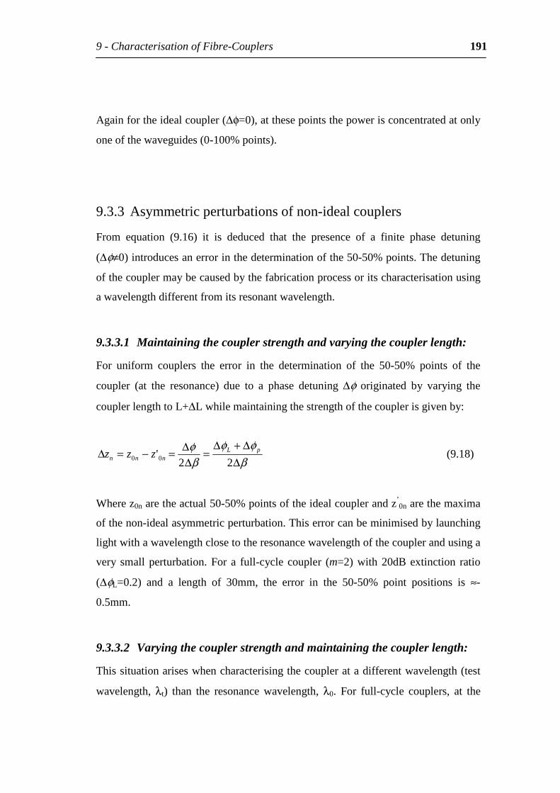
9-CharacterisationofFibre-Couplers 191
Againfortheidealcoupler(∆φ=0),atthesepointsthepowerisconcentratedatonly
oneofthewaveguides(0-100%points).
9.3.3 Asymmetricperturbationsofnon-idealcouplers
From equation (9.16) it is deduced that the presence of a finite phase detuning
(∆φ≠0)introducesanerrorinthedeterminationofthe50-50%points.Thedetuning
ofthecouplermaybecausedbythefabricationprocessoritscharacterisationusing
awavelengthdifferentfromitsresonantwavelength.
9.3.3.1 Maintainingthecouplerstrengthandvaryingthecouplerlength:
For uniform couplers the error in the determination of the 50-50% points of the
coupler (at the resonance) due to a phase detuning ∆φ originated by varying the
couplerlengthtoL+∆Lwhilemaintainingthestrengthofthecouplerisgivenby:
βφφ
βφ
∆∆+∆
=∆∆=−=∆
22'00
pLnnn zzz (9.18)
Wherez0naretheactual50-50%pointsoftheidealcouplerandz’0narethemaxima
ofthenon-idealasymmetricperturbation.Thiserrorcanbeminimisedbylaunching
lightwithawavelengthclosetotheresonancewavelengthofthecouplerandusinga
very small perturbation.For a full-cycle coupler (m=2)with20dBextinction ratio
(∆φL=0.2) and a length of 30mm, the error in the 50-50% point positions is ≈-
0.5mm.
9.3.3.2 Varyingthecouplerstrengthandmaintainingthecouplerlength:
Thissituationariseswhencharacterisingthecoupleratadifferentwavelength(test
wavelength, λt) than the resonance wavelength, λ0. For full-cycle couplers, at the
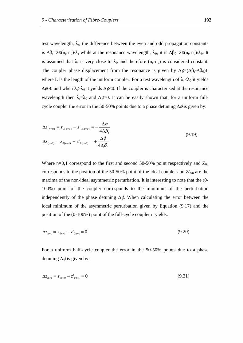
9-CharacterisationofFibre-Couplers 192
testwavelength,λt, thedifferencebetweentheevenandoddpropagationconstants
is∆βt=2π(ne-no)/λtwhileattheresonancewavelength,λ0, itis∆β0=2π(ne-no)/λ0.It
is assumed thatλt is very close to λ0 and therefore (ne-no) is considered constant.
The coupler phase displacement from the resonance is given by ∆φ=(∆βt-∆β0)L
whereListhelengthoftheuniformcoupler.Foratestwavelengthofλt<λ0ityields
∆φ>0andwhenλt>λ0ityields∆φ<0.Ifthecouplerischaracterisedattheresonance
wavelength then λt=λ0 and ∆φ=0. It can be easily shown that, for a uniform full-
cyclecouplertheerrorinthe50-50%pointsduetoaphasedetuning∆φisgivenby:
tnnn
tnnn
zzz
zzz
βφβφ
∆∆+=−=∆
∆∆−=−=∆
===
===
4'
4'
)1(0)1(0)1(
)0(0)0(0)0(
(9.19)
Wheren=0,1correspondtothefirstandsecond50-50%pointrespectivelyandZ0n
correspondstothepositionofthe50-50%pointoftheidealcouplerandZ’ 0narethe
maximaofthenon-idealasymmetricperturbation.Itisinterestingtonotethatthe(0-
100%) point of the coupler corresponds to the minimum of the perturbation
independently of the phase detuning ∆φ. When calculating the error between the
local minimum of the asymmetric perturbation given by Equation (9.17) and the
positionofthe(0-100%)pointofthefull-cyclecouplerityields:
0' 10101 =−=∆ === nnn zzz (9.20)
For a uniform half-cycle coupler the error in the 50-50% points due to a phase
detuning∆φisgivenby:
0' 00000 =−=∆ === nnn zzz (9.21)
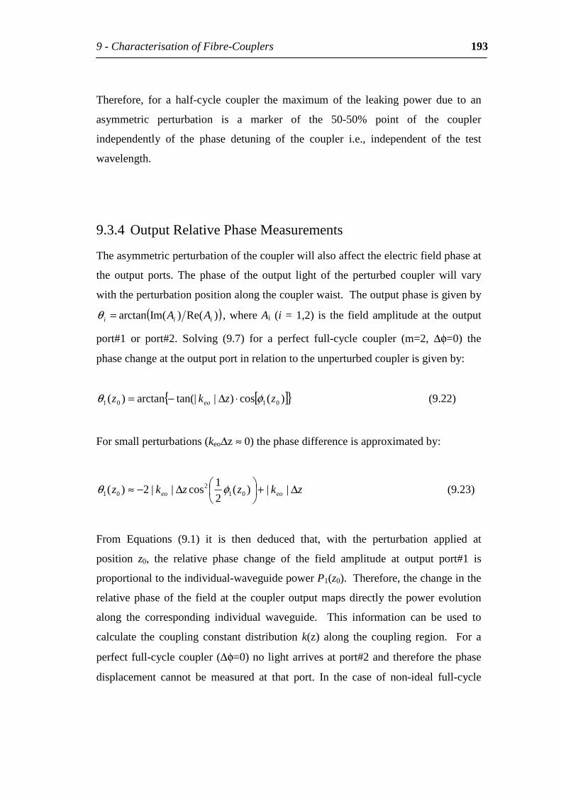
9-CharacterisationofFibre-Couplers 193
Therefore, for a half-cycle coupler the maximum of the leaking power due to an
asymmetric perturbation is a marker of the 50-50% point of the coupler
independently of the phase detuning of the coupler i.e., independent of the test
wavelength.
9.3.4 OutputRelativePhaseMeasurements
Theasymmetricperturbationofthecouplerwillalsoaffecttheelectricfieldphaseat
the output ports. The phase of the output light of the perturbed coupler will vary
withtheperturbationpositionalongthecouplerwaist.Theoutputphaseisgivenby
( ))Re()Im(arctan iii AA=θ ,whereAi (i=1,2) is the fieldamplitudeat theoutput
port#1 or port#2. Solving (9.7) for a perfect full-cycle coupler (m=2, ∆φ=0) the
phasechangeattheoutputportinrelationtotheunperturbedcouplerisgivenby:
[ ] )(cos)|tan(|arctan)( 0101 zzkz eo φθ ⋅∆−= (9.22)
Forsmallperturbations(keo∆z≈0)thephasedifferenceisapproximatedby:
zkzzkz eoeo ∆+
∆−≈ ||)(21
cos||2)( 012
01 φθ (9.23)
From Equations (9.1) it is then deduced that, with the perturbation applied at
position z0, the relative phase change of the field amplitude at output port#1 is
proportionaltotheindividual-waveguidepowerP1(z0).Therefore,thechangeinthe
relativephaseof the fieldat thecoupleroutputmapsdirectly thepowerevolution
along the corresponding individual waveguide. This information can be used to
calculate the coupling constant distribution k(z) along the coupling region. For a
perfectfull-cyclecoupler(∆φ=0)nolightarrivesatport#2andtherefore thephase
displacement cannot be measured at that port. In the case of non-ideal full-cycle
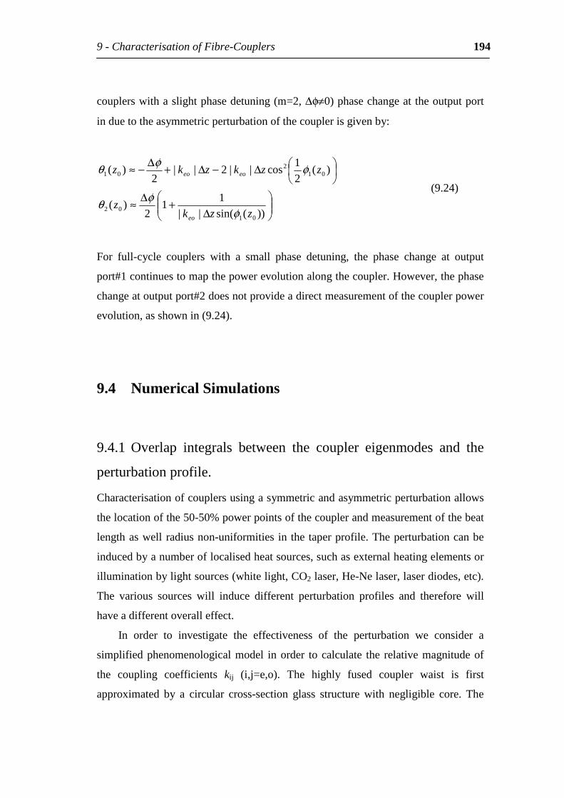
9-CharacterisationofFibre-Couplers 194
couplerswithaslightphasedetuning(m=2,∆φ≠0)phasechangeattheoutputport
induetotheasymmetricperturbationofthecouplerisgivenby:
∆+∆≈
∆−∆+∆−≈
))(sin(||1
12
)(
)(21
cos||2||2
)(
0102
012
01
zzkz
zzkzkz
eo
eoeo
φφθ
φφθ (9.24)
For full-cycle couplers with a small phase detuning, the phase change at output
port#1continuestomapthepowerevolutionalongthecoupler.However,thephase
changeatoutputport#2doesnotprovideadirectmeasurementofthecouplerpower
evolution,asshownin(9.24).
9.4 NumericalSimulations
9.4.1 Overlap integrals between the coupler eigenmodes and the
perturbationprofile.
Characterisationofcouplersusingasymmetricandasymmetricperturbationallows
thelocationofthe50-50%powerpointsofthecouplerandmeasurementofthebeat
lengthaswell radiusnon-uniformities inthetaperprofile.Theperturbationcanbe
inducedbyanumberoflocalisedheatsources,suchasexternalheatingelementsor
illuminationbylightsources(whitelight,CO2laser,He-Nelaser,laserdiodes,etc).
The various sources will induce different perturbation profiles and therefore will
haveadifferentoveralleffect.
In order to investigate the effectiveness of the perturbation we consider a
simplifiedphenomenologicalmodel inorder tocalculate the relativemagnitudeof
the coupling coefficients kij (i,j=e,o). The highly fused coupler waist is first
approximated by a circular cross-section glass structure with negligible core. The
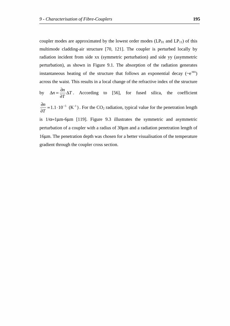
9-CharacterisationofFibre-Couplers 195
couplermodesareapproximatedbythelowestordermodes(LP01andLP11)ofthis
multimode cladding-air structure [70, 121]. The coupler is perturbed locally by
radiation incident from side xx (symmetric perturbation) and side yy (asymmetric
perturbation), as shown in Figure 9.1. The absorption of the radiation generates
instantaneous heating of the structure that follows an exponential decay (~e-αx)
acrossthewaist.Thisresultsinalocalchangeoftherefractiveindexofthestructure
by TTn
n ∆∂∂=∆ . According to [56], for fused silica, the coefficient
)(K101.1 1-5−⋅≈∂∂Tn
.FortheCO2radiation,typicalvalueforthepenetrationlength
is 1/α≈1µm-6µm [119]. Figure 9.3 illustrates the symmetric and asymmetric
perturbationofacouplerwitharadiusof30µmandaradiationpenetrationlengthof
16µm.Thepenetrationdepthwaschosenforabettervisualisationofthetemperature
gradientthroughthecouplercrosssection.
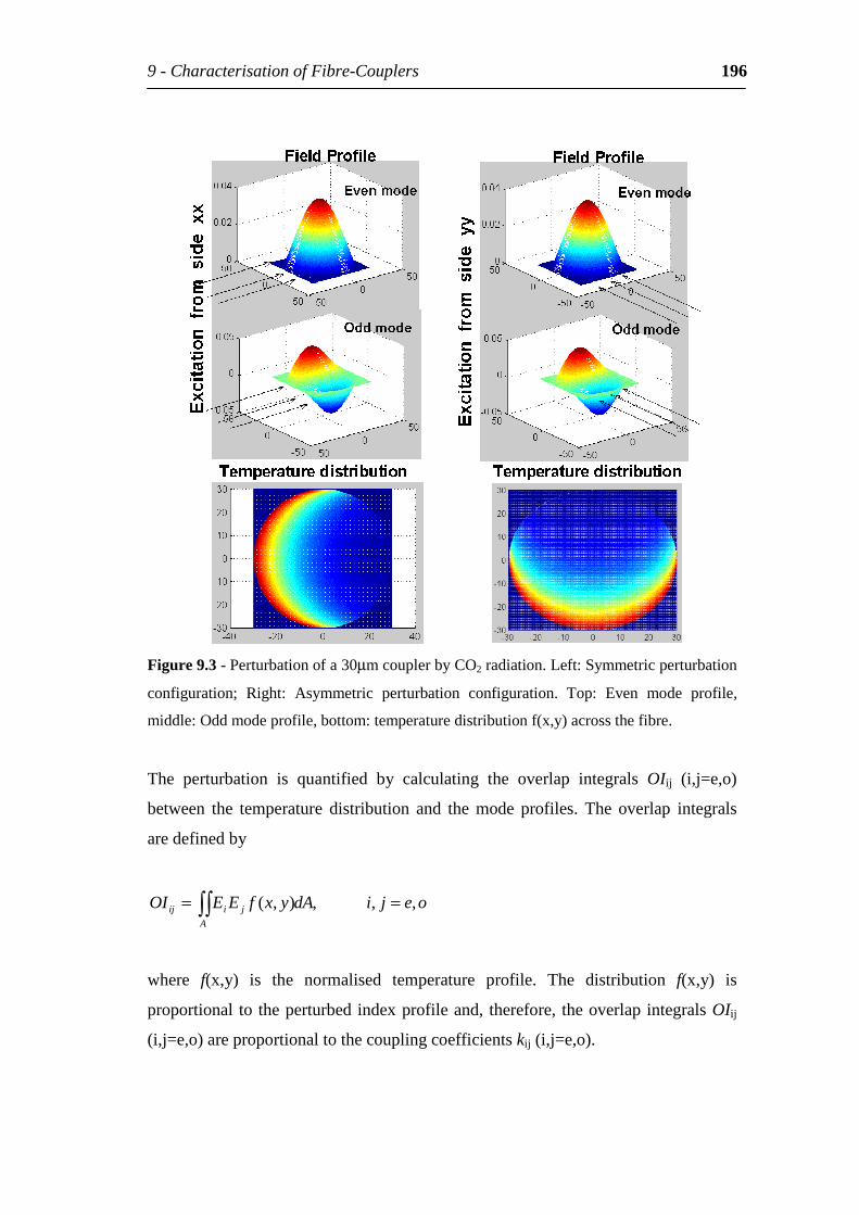
9-CharacterisationofFibre-Couplers 196
Figure9.3-Perturbationofa30µmcouplerbyCO2radiation.Left:Symmetricperturbation
configuration; Right: Asymmetric perturbation configuration. Top: Even mode profile,
middle:Oddmodeprofile,bottom:temperaturedistributionf(x,y)acrossthefibre.
The perturbation is quantified by calculating the overlap integrals OIij (i,j=e,o)
between the temperature distribution and the mode profiles. The overlap integrals
aredefinedby
oejidAyxfEEOIA
jiij ,,,),( ==
where f(x,y) is the normalised temperature profile. The distribution f(x,y) is
proportional totheperturbedindexprofileand, therefore, theoverlapintegralsOIij
(i,j=e,o)areproportionaltothecouplingcoefficientskij(i,j=e,o).
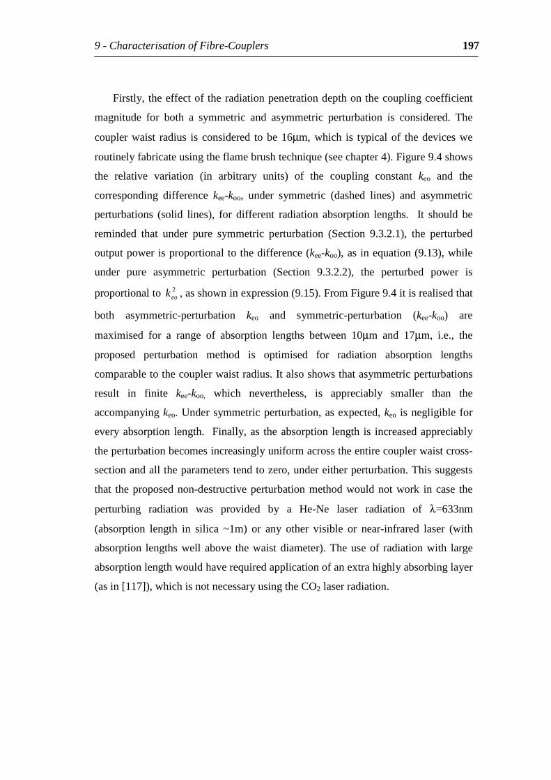
9-CharacterisationofFibre-Couplers 197
Firstly,theeffectoftheradiationpenetrationdepthonthecouplingcoefficient
magnitude for both a symmetric and asymmetric perturbation is considered. The
couplerwaist radius is considered tobe16µm,which is typicalof thedeviceswe
routinelyfabricateusingtheflamebrushtechnique(seechapter4).Figure9.4shows
the relative variation (in arbitrary units) of the coupling constant keo and the
corresponding difference kee-koo, under symmetric (dashed lines) and asymmetric
perturbations (solid lines), for different radiation absorption lengths. It should be
reminded that under pure symmetric perturbation (Section 9.3.2.1), the perturbed
outputpowerisproportionaltothedifference(kee-koo),asinequation(9.13),while
under pure asymmetric perturbation (Section 9.3.2.2), the perturbed power is
proportionalto 2eok ,asshowninexpression(9.15).FromFigure9.4itisrealisedthat
both asymmetric-perturbation keo and symmetric-perturbation (kee-koo) are
maximised for a range of absorption lengths between 10µm and 17µm, i.e., the
proposed perturbation method is optimised for radiation absorption lengths
comparabletothecouplerwaistradius.Italsoshowsthatasymmetricperturbations
result in finite kee-koo, which nevertheless, is appreciably smaller than the
accompanyingkeo.Undersymmetricperturbation,asexpected,keo isnegligible for
everyabsorption length. Finally,as theabsorption length is increasedappreciably
theperturbationbecomesincreasinglyuniformacrosstheentirecouplerwaistcross-
sectionandalltheparameterstendtozero,undereitherperturbation.Thissuggests
that theproposednon-destructiveperturbationmethodwouldnotwork incase the
perturbing radiation was provided by a He-Ne laser radiation of λ=633nm
(absorption length in silica ~1m) or any other visible or near-infrared laser (with
absorption lengthswell above thewaistdiameter).Theuseof radiationwith large
absorptionlengthwouldhaverequiredapplicationofanextrahighlyabsorbinglayer
(asin[117]),whichisnotnecessaryusingtheCO2laserradiation.
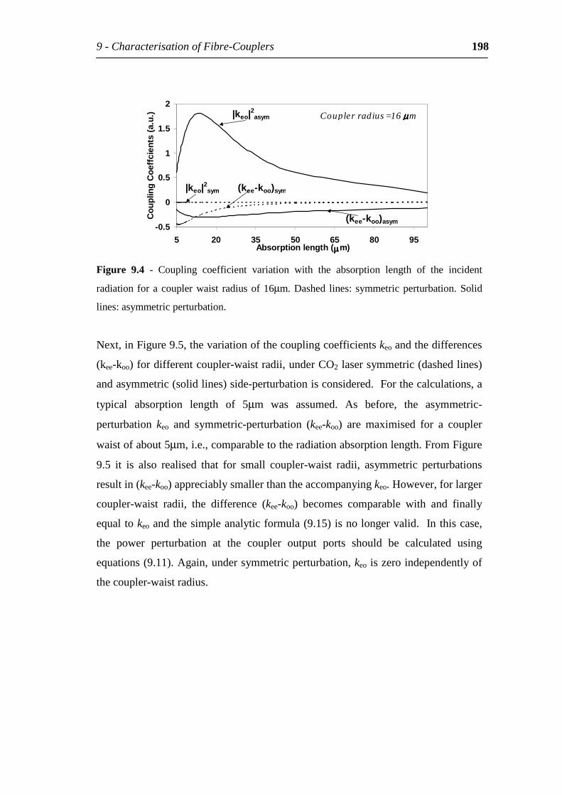
9-CharacterisationofFibre-Couplers 198
-0.5
0
0.5
1
1.5
2
5 20 35 50 65 80 95Absorptionlength(µµµµm)
Cou
plin
gC
oeff
cien
ts(
a.u.
)
(kee-koo)sym
|keo|2asym
|keo|2sym
(kee-koo)asym
Coupler radius=16 µµµµm
Figure 9.4 - Coupling coefficient variation with the absorption length of the incident
radiationforacouplerwaist radiusof16µm.Dashed lines:symmetricperturbation.Solid
lines:asymmetricperturbation.
Next,inFigure9.5,thevariationofthecouplingcoefficientskeoandthedifferences
(kee-koo)fordifferentcoupler-waistradii,underCO2lasersymmetric(dashedlines)
andasymmetric(solidlines)side-perturbationisconsidered.Forthecalculations,a
typical absorption length of 5µm was assumed. As before, the asymmetric-
perturbation keo and symmetric-perturbation (kee-koo) are maximised for a coupler
waistofabout5µm,i.e.,comparabletotheradiationabsorptionlength.FromFigure
9.5 it is also realised that for small coupler-waist radii, asymmetric perturbations
resultin(kee-koo)appreciablysmallerthantheaccompanyingkeo.However,forlarger
coupler-waist radii, the difference (kee-koo) becomes comparable with and finally
equaltokeoandthesimpleanalyticformula(9.15)isnolongervalid.Inthiscase,
the power perturbation at the coupler output ports should be calculated using
equations(9.11).Again,undersymmetricperturbation,keoiszeroindependentlyof
thecoupler-waistradius.
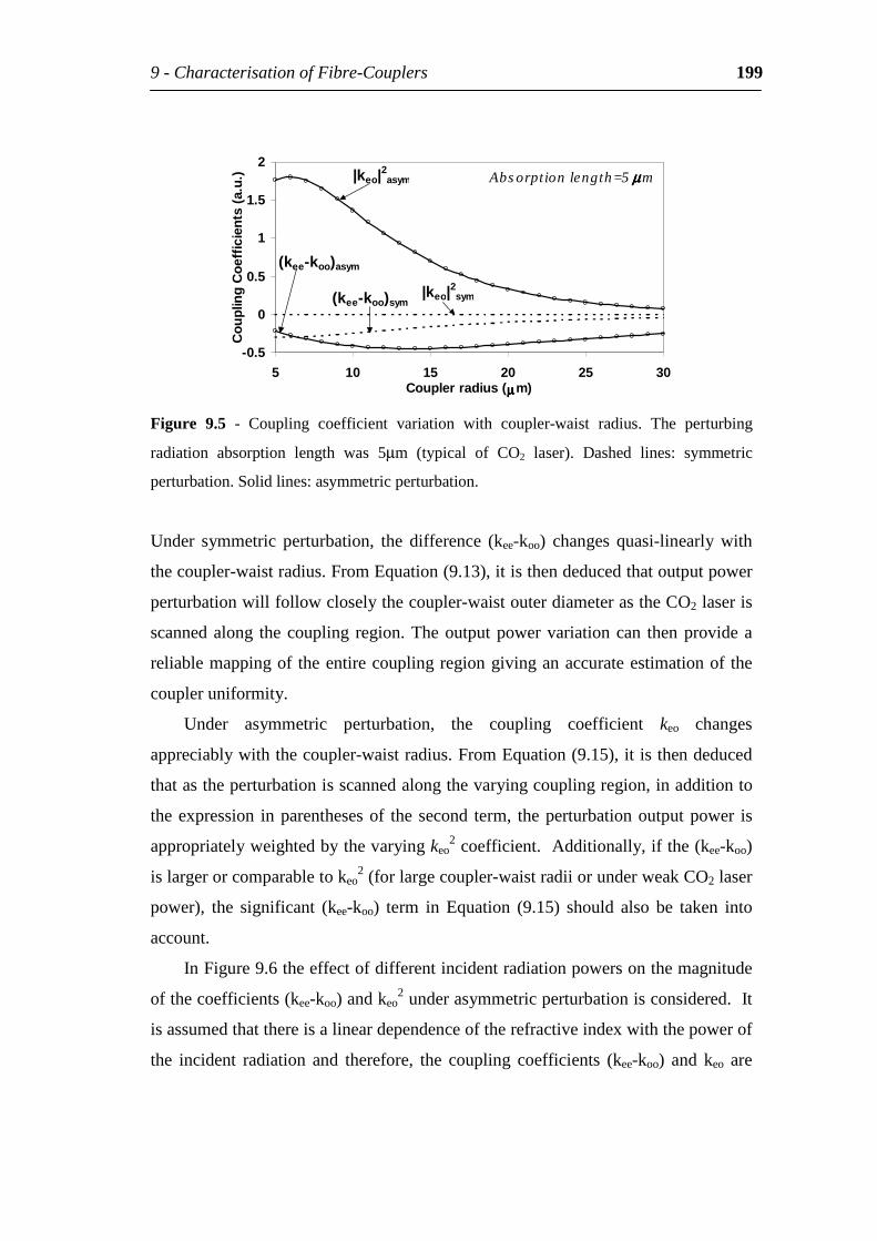
9-CharacterisationofFibre-Couplers 199
-0.5
0
0.5
1
1.5
2
5 10 15 20 25 30Couplerradius(µµµµm)
Cou
plin
gC
oeff
icie
nts
(a.u
.)
(kee-koo)sym
|keo|2asym
|keo|2sym
(kee-koo)asym
Absorption length=5 µµµµm
Figure 9.5 - Coupling coefficient variation with coupler-waist radius. The perturbing
radiation absorption length was 5µm (typical of CO2 laser). Dashed lines: symmetric
perturbation.Solidlines:asymmetricperturbation.
Under symmetric perturbation, the difference (kee-koo) changes quasi-linearly with
thecoupler-waistradius.FromEquation(9.13),itisthendeducedthatoutputpower
perturbationwillfollowcloselythecoupler-waistouterdiameterastheCO2laseris
scannedalong thecoupling region.Theoutputpowervariationcan thenprovidea
reliablemappingof theentirecouplingregiongivinganaccurateestimationof the
coupleruniformity.
Under asymmetric perturbation, the coupling coefficient keo changes
appreciablywiththecoupler-waistradius.FromEquation(9.15),itisthendeduced
thatastheperturbationisscannedalongthevaryingcouplingregion,inadditionto
theexpression inparenthesesof the second term, theperturbationoutputpower is
appropriatelyweightedbythevaryingkeo2coefficient.Additionally,ifthe(kee-koo)
islargerorcomparabletokeo2(forlargecoupler-waistradiiorunderweakCO2laser
power), the significant (kee-koo) term in Equation (9.15) should also be taken into
account.
InFigure9.6theeffectofdifferentincidentradiationpowersonthemagnitude
ofthecoefficients(kee-koo)andkeo2underasymmetricperturbationisconsidered.It
isassumedthatthereisalineardependenceoftherefractiveindexwiththepowerof
the incident radiation and therefore, the coupling coefficients (kee-koo) and keo are
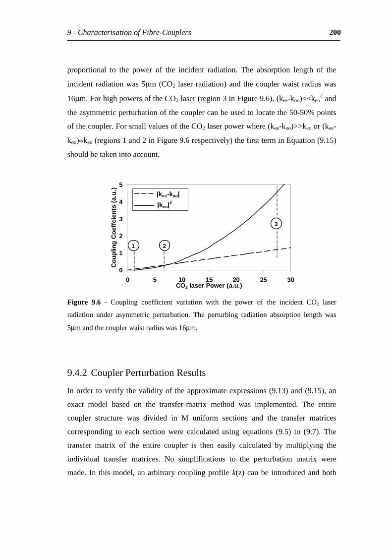
9-CharacterisationofFibre-Couplers 200
proportional to the power of the incident radiation. The absorption length of the
incident radiationwas5µm(CO2 laser radiation)and thecouplerwaist radiuswas
16µm.ForhighpowersoftheCO2laser(region3inFigure9.6),(kee-koo)<<keo2and
theasymmetricperturbationofthecouplercanbeusedtolocatethe50-50%points
ofthecoupler.ForsmallvaluesoftheCO2laserpowerwhere(kee-koo)>>keoor(kee-
koo)≈keo(regions1and2inFigure9.6respectively)thefirstterminEquation(9.15)
shouldbetakenintoaccount.
0
1
2
3
4
5
0 5 10 15 20 25 30CO2laserPower(a.u.)
Cou
plin
gC
oeff
cien
ts(
a.u.
)
|keo|2
|kee-koo|
1
3
2
Figure 9.6 - Coupling coefficient variation with the power of the incident CO2 laser
radiation under asymmetric perturbation. The perturbing radiation absorption length was
5µmandthecouplerwaistradiuswas16µm.
9.4.2 CouplerPerturbationResults
Inorder toverifythevalidityof theapproximateexpressions(9.13)and(9.15),an
exact model based on the transfer-matrix method was implemented. The entire
coupler structure was divided in M uniform sections and the transfer matrices
corresponding to each section were calculated using equations (9.5) to (9.7). The
transfer matrix of the entire coupler is then easily calculated by multiplying the
individual transfer matrices. No simplifications to the perturbation matrix were
made. In thismodel, anarbitrarycouplingprofilek(z)canbe introducedandboth
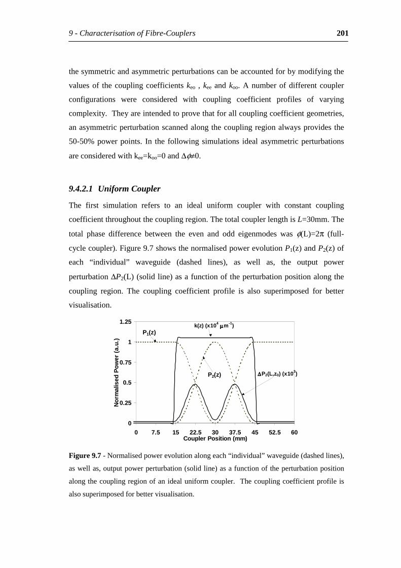
9-CharacterisationofFibre-Couplers 201
thesymmetricandasymmetricperturbationscanbeaccountedforbymodifyingthe
valuesof thecouplingcoefficientskeo ,kee andkoo.Anumberofdifferentcoupler
configurations were considered with coupling coefficient profiles of varying
complexity.Theyareintendedtoprovethatforallcouplingcoefficientgeometries,
anasymmetricperturbationscannedalongthecouplingregionalwaysprovidesthe
50-50%powerpoints. In the followingsimulations idealasymmetricperturbations
areconsideredwithkee=koo=0and∆φ≠0.
9.4.2.1 UniformCoupler
The first simulation refers to an ideal uniform coupler with constant coupling
coefficientthroughoutthecouplingregion.ThetotalcouplerlengthisL=30mm.The
total phase difference between the even and odd eigenmodes was φ(L)=2π (full-
cyclecoupler).Figure9.7showsthenormalisedpowerevolutionP1(z)andP2(z)of
each “individual” waveguide (dashed lines), as well as, the output power
perturbation∆P2(L)(solidline)asafunctionoftheperturbationpositionalongthe
coupling region. The coupling coefficient profile is also superimposed for better
visualisation.
0
0.25
0.5
0.75
1
1.25
0 7.5 15 22.5 30 37.5 45 52.5 60CouplerPosition(mm)
Nor
mal
ised
Pow
er(
a.u.
)
P1(z)
P2(z) ∆∆∆∆P2(L,z0)(x103)
k(z)(x104µµµµm-1)
Figure9.7-Normalisedpowerevolutionalongeach“individual”waveguide(dashedlines),
aswellas,outputpowerperturbation(solidline)asafunctionoftheperturbationposition
alongthecouplingregionofanidealuniformcoupler. Thecouplingcoefficientprofileis
alsosuperimposedforbettervisualisation.
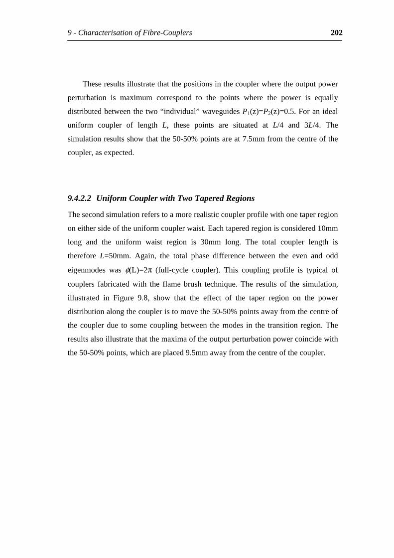
9-CharacterisationofFibre-Couplers 202
Theseresultsillustratethatthepositionsinthecouplerwheretheoutputpower
perturbation is maximum correspond to the points where the power is equally
distributedbetweenthetwo“ individual” waveguidesP1(z)=P2(z)=0.5.Foranideal
uniform coupler of length L, these points are situated at L/4 and 3L/4. The
simulationresultsshowthatthe50-50%pointsareat7.5mmfromthecentreofthe
coupler,asexpected.
9.4.2.2 UniformCouplerwithTwoTaperedRegions
Thesecondsimulationreferstoamorerealisticcouplerprofilewithonetaperregion
oneithersideoftheuniformcouplerwaist.Eachtaperedregionisconsidered10mm
long and the uniform waist region is 30mm long. The total coupler length is
therefore L=50mm. Again, the total phase difference between the even and odd
eigenmodes was φ(L)=2π (full-cycle coupler). This coupling profile is typical of
couplers fabricated with the flame brush technique. The results of the simulation,
illustrated in Figure 9.8, show that the effect of the taper region on the power
distributionalongthecoupleristomovethe50-50%pointsawayfromthecentreof
thecouplerdue to somecouplingbetween themodes in the transition region.The
resultsalsoillustratethatthemaximaoftheoutputperturbationpowercoincidewith
the50-50%points,whichareplaced9.5mmawayfromthecentreofthecoupler.
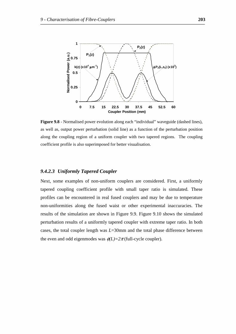
9-CharacterisationofFibre-Couplers 203
0
0.25
0.5
0.75
1
0 7.5 15 22.5 30 37.5 45 52.5 60CouplerPosition(mm)
Nor
mal
ised
Pow
er(
a.u.
)∆∆∆∆P2(L,z0)(x103)
P1(z)
P2(z)
k(z)(x104µµµµm-1)
Figure9.8-Normalisedpowerevolutionalongeach“ individual” waveguide(dashedlines),
aswellas,outputpowerperturbation(solidline)asafunctionoftheperturbationposition
along the coupling region of a uniform coupler with two tapered regions. The coupling
coefficientprofileisalsosuperimposedforbettervisualisation.
9.4.2.3 UniformlyTaperedCoupler
Next, some examples of non-uniform couplers are considered. First, a uniformly
tapered coupling coefficient profile with small taper ratio is simulated. These
profiles canbe encountered in real fused couplers andmaybedue to temperature
non-uniformities along the fused waist or other experimental inaccuracies. The
resultsof thesimulationareshowninFigure9.9.Figure9.10showsthesimulated
perturbationresultsofauniformlytaperedcouplerwithextremetaperratio.Inboth
cases,thetotalcouplerlengthwasL=30mmandthetotalphasedifferencebetween
theevenandoddeigenmodeswasφ(L)=2π(full-cyclecoupler).
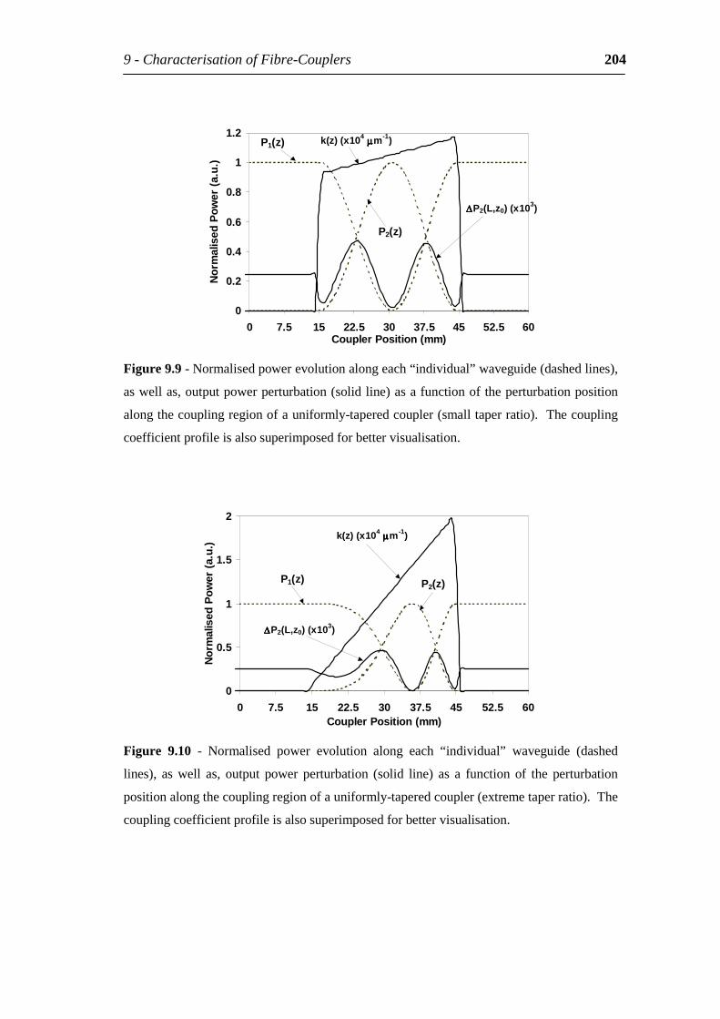
9-CharacterisationofFibre-Couplers 204
0
0.2
0.4
0.6
0.8
1
1.2
0 7.5 15 22.5 30 37.5 45 52.5 60CouplerPosition(mm)
Nor
mal
ised
Pow
er(
a.u.
)
P1(z)
P2(z)
∆∆∆∆P2(L,z0)(x103)
k(z)(x104µµµµm-1)
Figure9.9-Normalisedpowerevolutionalongeach“ individual” waveguide(dashedlines),
aswellas,outputpowerperturbation(solidline)asafunctionoftheperturbationposition
alongthecouplingregionofauniformly-taperedcoupler(smalltaperratio).Thecoupling
coefficientprofileisalsosuperimposedforbettervisualisation.
0
0.5
1
1.5
2
0 7.5 15 22.5 30 37.5 45 52.5 60CouplerPosition(mm)
Nor
mal
ised
Pow
er(
a.u.
)
∆∆∆∆P2(L,z0)(x103)
P1(z) P2(z)
k(z)(x104µµµµm-1)
Figure 9.10 - Normalised power evolution along each “ individual” waveguide (dashed
lines), as well as, output power perturbation (solid line) as a function of the perturbation
positionalongthecouplingregionofauniformly-taperedcoupler(extremetaperratio).The
couplingcoefficientprofileisalsosuperimposedforbettervisualisation.
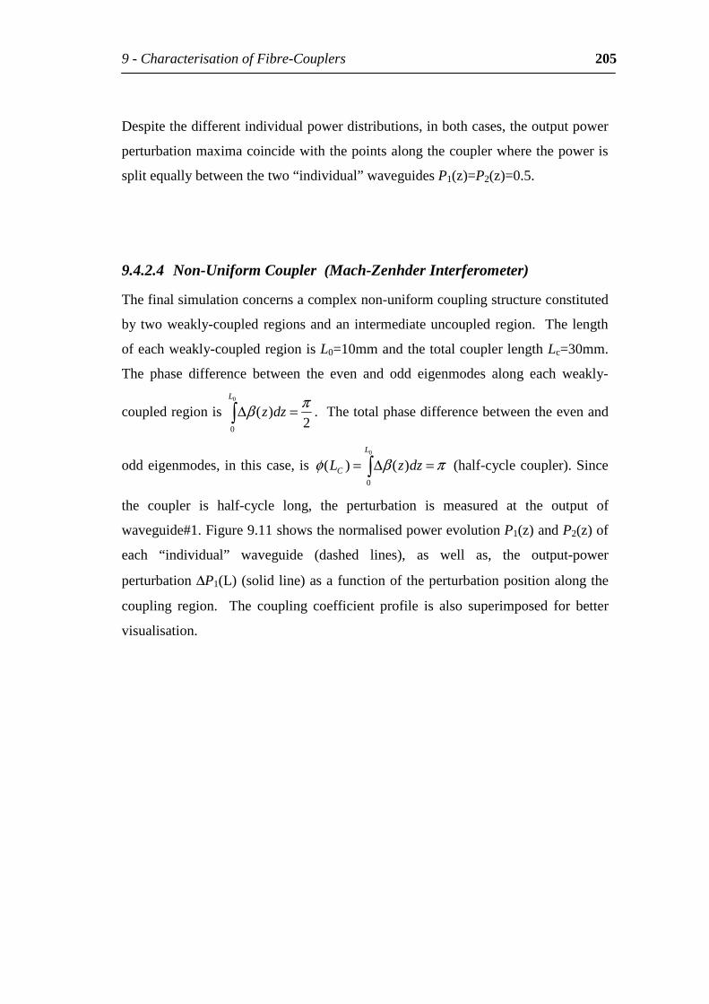
9-CharacterisationofFibre-Couplers 205
Despitethedifferentindividualpowerdistributions,inbothcases,theoutputpower
perturbationmaximacoincidewiththepointsalongthecouplerwherethepoweris
splitequallybetweenthetwo“ individual” waveguidesP1(z)=P2(z)=0.5.
9.4.2.4 Non-UniformCoupler(Mach-ZenhderInterferometer)
Thefinalsimulationconcernsacomplexnon-uniformcouplingstructureconstituted
bytwoweakly-coupledregionsandanintermediateuncoupledregion. Thelength
ofeachweakly-coupledregionisL0=10mmandthetotalcouplerlengthLc=30mm.
The phase difference between the even and odd eigenmodes along each weakly-
coupledregionis2
)(0
0
πβ =∆L
dzz .Thetotalphasedifferencebetweentheevenand
oddeigenmodes, in thiscase, is πβφ =∆= 0
0
)()(L
C dzzL (half-cyclecoupler).Since
the coupler is half-cycle long, the perturbation is measured at the output of
waveguide#1.Figure9.11showsthenormalisedpowerevolutionP1(z)andP2(z)of
each “ individual” waveguide (dashed lines), as well as, the output-power
perturbation∆P1(L)(solidline)asafunctionoftheperturbationpositionalongthe
coupling region. The coupling coefficient profile is also superimposed for better
visualisation.
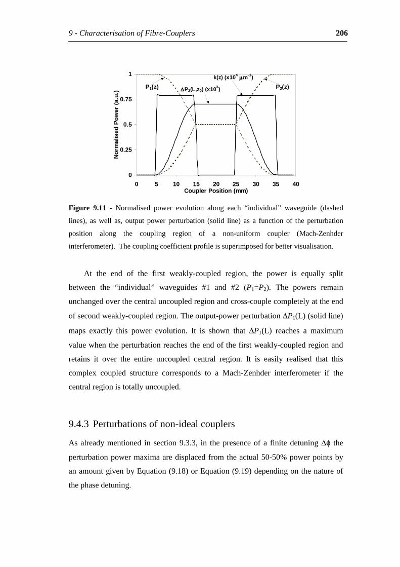
9-CharacterisationofFibre-Couplers 206
0
0.25
0.5
0.75
1
0 5 10 15 20 25 30 35 40CouplerPosition(mm)
Nor
mal
ised
Pow
er(
a.u.
) ∆∆∆∆P2(L,z0)(x103) P2(z)P1(z)
k(z)(x104µµµµm-1)
Figure 9.11 - Normalised power evolution along each “ individual” waveguide (dashed
lines), as well as, output power perturbation (solid line) as a function of the perturbation
position along the coupling region of a non-uniform coupler (Mach-Zenhder
interferometer).Thecouplingcoefficientprofileissuperimposedforbettervisualisation.
At the end of the first weakly-coupled region, the power is equally split
between the “ individual” waveguides #1 and #2 (P1=P2). The powers remain
unchangedoverthecentraluncoupledregionandcross-couplecompletelyattheend
ofsecondweakly-coupledregion.Theoutput-powerperturbation∆P1(L)(solidline)
maps exactly this power evolution. It is shown that ∆P1(L) reaches a maximum
valuewhentheperturbationreachestheendofthefirstweakly-coupledregionand
retains it over the entire uncoupled central region. It is easily realised that this
complex coupled structure corresponds to a Mach-Zenhder interferometer if the
centralregionistotallyuncoupled.
9.4.3 Perturbationsofnon-idealcouplers
Asalreadymentioned in section9.3.3, in thepresenceof a finitedetuning∆φ the
perturbationpowermaximaaredisplacedfromtheactual50-50%powerpointsby
anamountgivenbyEquation(9.18)orEquation(9.19)dependingonthenatureof
thephasedetuning.
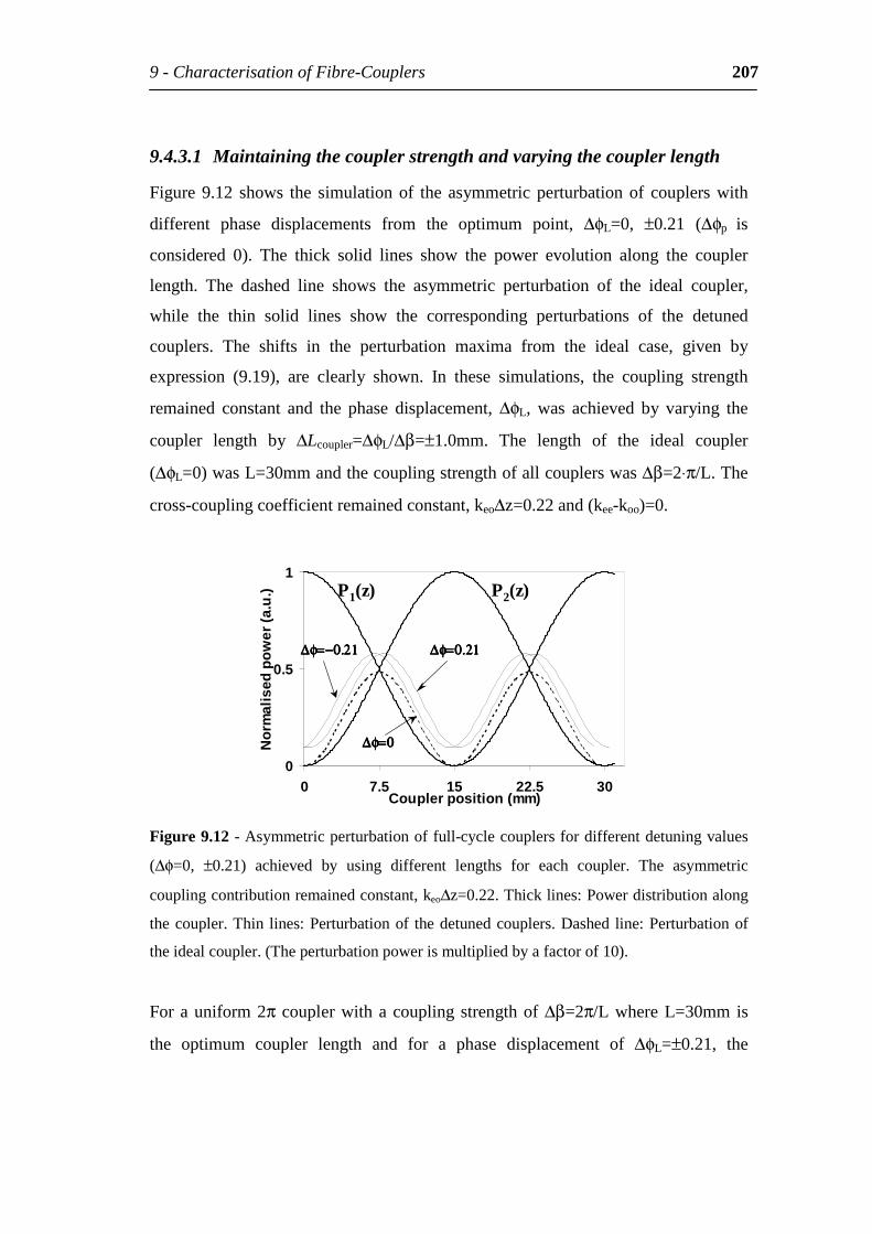
9-CharacterisationofFibre-Couplers 207
9.4.3.1 Maintainingthecouplerstrengthandvaryingthecouplerlength
Figure9.12 shows the simulationof the asymmetricperturbationof couplerswith
different phase displacements from the optimum point, ∆φL=0, ±0.21 (∆φp is
considered 0). The thick solid lines show the power evolution along the coupler
length. The dashed line shows the asymmetric perturbation of the ideal coupler,
while the thin solid lines show the corresponding perturbations of the detuned
couplers. The shifts in the perturbation maxima from the ideal case, given by
expression (9.19), are clearly shown. In these simulations, the coupling strength
remained constant and the phase displacement, ∆φL, was achieved by varying the
coupler length by ∆Lcoupler=∆φL/∆β=±1.0mm. The length of the ideal coupler
(∆φL=0)wasL=30mmandthecouplingstrengthofallcouplerswas∆β=2⋅π/L.The
cross-couplingcoefficientremainedconstant,keo∆z=0.22and(kee-koo)=0.
0
0.5
1
0 7.5 15 22.5 30Couplerposition(mm)
Nor
mal
ised
pow
er(a
.u.)
∆φ∆φ∆φ∆φ====−−−−0.210.210.210.21 ∆φ∆φ∆φ∆φ=0.21=0.21=0.21=0.21
∆φ∆φ∆φ∆φ=0=0=0=0
P2(z)P1(z)
0
0.5
1
0 7.5 15 22.5 30Couplerposition(mm)
Nor
mal
ised
pow
er(a
.u.)
∆φ∆φ∆φ∆φ====−−−−0.210.210.210.21 ∆φ∆φ∆φ∆φ=0.21=0.21=0.21=0.21
∆φ∆φ∆φ∆φ=0=0=0=0
P2(z)P1(z)
Figure9.12-Asymmetricperturbationoffull-cyclecouplersfordifferentdetuningvalues
(∆φ=0, ±0.21) achieved by using different lengths for each coupler. The asymmetric
couplingcontributionremainedconstant,keo∆z=0.22.Thicklines:Powerdistributionalong
thecoupler.Thinlines:Perturbationof thedetunedcouplers.Dashed line:Perturbationof
theidealcoupler.(Theperturbationpowerismultipliedbyafactorof10).
Forauniform2π couplerwithacouplingstrengthof∆β=2π/LwhereL=30mmis
the optimum coupler length and for a phase displacement of ∆φL=±0.21, the
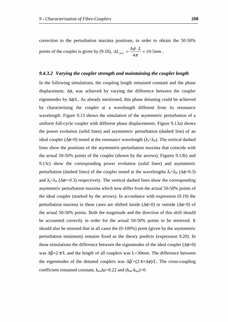
9-CharacterisationofFibre-Couplers 208
correction to the perturbation maxima positions, in order to obtain the 50-50%
pointsofthecouplerisgivenby(9.18), mmL
L pert 5.04
±≈⋅∆=∆π
φ.
9.4.3.2 Varyingthecouplerstrengthandmaintainingthecouplerlength
In the followingsimulations, thecoupling length remainedconstant and thephase
displacement, ∆φ, was achieved by varying the difference between the coupler
eigenmodesby∆φ/L.Asalreadymentioned,thisphasedetuningcouldbeachieved
by characterising the coupler at a wavelength different from its resonance
wavelength.Figure9.13shows the simulationof theasymmetricperturbationofa
uniformfull-cyclecouplerwithdifferentphasedisplacements.Figure9.13a)shows
the power evolution (solid lines) and asymmetric perturbation (dashed line) of an
idealcoupler(∆φ=0)testedattheresonancewavelength(λt=λ0).Theverticaldashed
linesshowthepositionsof theasymmetric-perturbationmaximathatcoincidewith
theactual50-50%pointsofthecoupler(shownbythearrows).Figures9.13b)and
9.13c) show the corresponding power evolution (solid lines) and asymmetric
perturbation(dashedlines)ofthecouplertestedatthewavelengthsλt<λ0(∆φ=0.3)
andλt>λ0(∆φ=-0.3)respectively.Theverticaldashedlinesshowthecorresponding
asymmetricperturbationmaximawhichnowdifferfromtheactual50-50%pointsof
theidealcoupler(markedbythearrows).Inaccordancewithexpression(9.19)the
perturbationmaxima in thesecasesare shifted inside (∆φ>0)oroutside (∆φ<0)of
theactual50-50%points.Boththemagnitudeandthedirectionofthisshiftshould
be accounted correctly in order for the actual 50-50% points to be retrieved. It
shouldalsobestressedthatinallcasesthe(0-100%)point(givenbytheasymmetric
perturbation minimum) remains fixed as the theory predicts (expression 9.20). In
thesesimulationsthedifferencebetweentheeigenmodesoftheidealcoupler(∆φ=0)
was∆β=2⋅π/LandthelengthofallcouplerswasL=30mm.Thedifferencebetween
the eigenmodes of the detuned couplers was ∆β’=(2⋅π+∆φ)/L. The cross-coupling
coefficientremainedconstant,keo∆z=0.22and(kee-koo)=0.
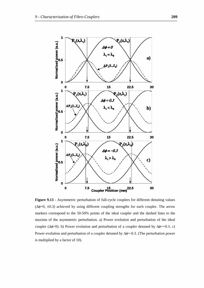
9-CharacterisationofFibre-Couplers 209
0
0.5
1
0 7.5 15 22.5 30
Nor
mal
ised
pow
er(a
.u.)
P2(z,λλλλt)P1(z,λλλλt)
b)∆∆∆∆P2(L,Z0)∆φ∆φ∆φ∆φ = 0.3= 0.3= 0.3= 0.3
λλλλ t < λ< λ< λ< λ0
0
0.5
1
0 7.5 15 22.5 30
Nor
mal
ised
pow
er(a
.u.)
P1(z,λλλλt) P2(z,λλλλt)
a)∆∆∆∆P2(L,Z0)
∆φ∆φ∆φ∆φ = 0= 0= 0= 0
λλλλ t = λ= λ= λ= λ0
0
0.5
1
0 7.5 15 22.5 30CouplerPosition(mm)
Nor
mal
ised
pow
er(a
.u.)
P1(z,λλλλ0) P2(z,λλλλ0)
c)
∆φ∆φ∆φ∆φ = = = = −−−−0.30.30.30.3
λλλλ t > λ> λ> λ> λ0
∆∆∆∆P2(L,Z0)
0
0.5
1
0 7.5 15 22.5 30
Nor
mal
ised
pow
er(a
.u.)
P2(z,λλλλt)P1(z,λλλλt)
b)∆∆∆∆P2(L,Z0)∆φ∆φ∆φ∆φ = 0.3= 0.3= 0.3= 0.3
λλλλ t < λ< λ< λ< λ0
0
0.5
1
0 7.5 15 22.5 30
Nor
mal
ised
pow
er(a
.u.)
P2(z,λλλλt)P1(z,λλλλt)
b)∆∆∆∆P2(L,Z0)∆φ∆φ∆φ∆φ = 0.3= 0.3= 0.3= 0.3
λλλλ t < λ< λ< λ< λ0
∆φ∆φ∆φ∆φ = 0.3= 0.3= 0.3= 0.3
λλλλ t < λ< λ< λ< λ0
0
0.5
1
0 7.5 15 22.5 30
Nor
mal
ised
pow
er(a
.u.)
P1(z,λλλλt) P2(z,λλλλt)
a)∆∆∆∆P2(L,Z0)
∆φ∆φ∆φ∆φ = 0= 0= 0= 0
λλλλ t = λ= λ= λ= λ0
0
0.5
1
0 7.5 15 22.5 30
Nor
mal
ised
pow
er(a
.u.)
P1(z,λλλλt) P2(z,λλλλt)
a)∆∆∆∆P2(L,Z0)
∆φ∆φ∆φ∆φ = 0= 0= 0= 0
λλλλ t = λ= λ= λ= λ0
∆φ∆φ∆φ∆φ = 0= 0= 0= 0
λλλλ t = λ= λ= λ= λ0
0
0.5
1
0 7.5 15 22.5 30CouplerPosition(mm)
Nor
mal
ised
pow
er(a
.u.)
P1(z,λλλλ0) P2(z,λλλλ0)
c)
∆φ∆φ∆φ∆φ = = = = −−−−0.30.30.30.3
λλλλ t > λ> λ> λ> λ0
∆∆∆∆P2(L,Z0)
0
0.5
1
0 7.5 15 22.5 30CouplerPosition(mm)
Nor
mal
ised
pow
er(a
.u.)
P1(z,λλλλ0) P2(z,λλλλ0)
c)
∆φ∆φ∆φ∆φ = = = = −−−−0.30.30.30.3
λλλλ t > λ> λ> λ> λ0
∆φ∆φ∆φ∆φ = = = = −−−−0.30.30.30.3
λλλλ t > λ> λ> λ> λ0
∆∆∆∆P2(L,Z0)
Figure9.13-Asymmetricperturbationoffull-cyclecouplersfordifferentdetuningvalues
(∆φ=0, ±0.3) achieved by using different coupling strengths for each coupler. The arrow
markers correspond to the50-50%pointsof the ideal coupler and thedashed lines to the
maxima of the asymmetric perturbation. a) Power evolution and perturbation of the ideal
coupler(∆φ=0).b)Powerevolutionandperturbationofacouplerdetunedby∆φ=+0.3.c)
Powerevolutionandperturbationofacouplerdetunedby∆φ=-0.3.(Theperturbationpower
ismultipliedbyafactorof10).
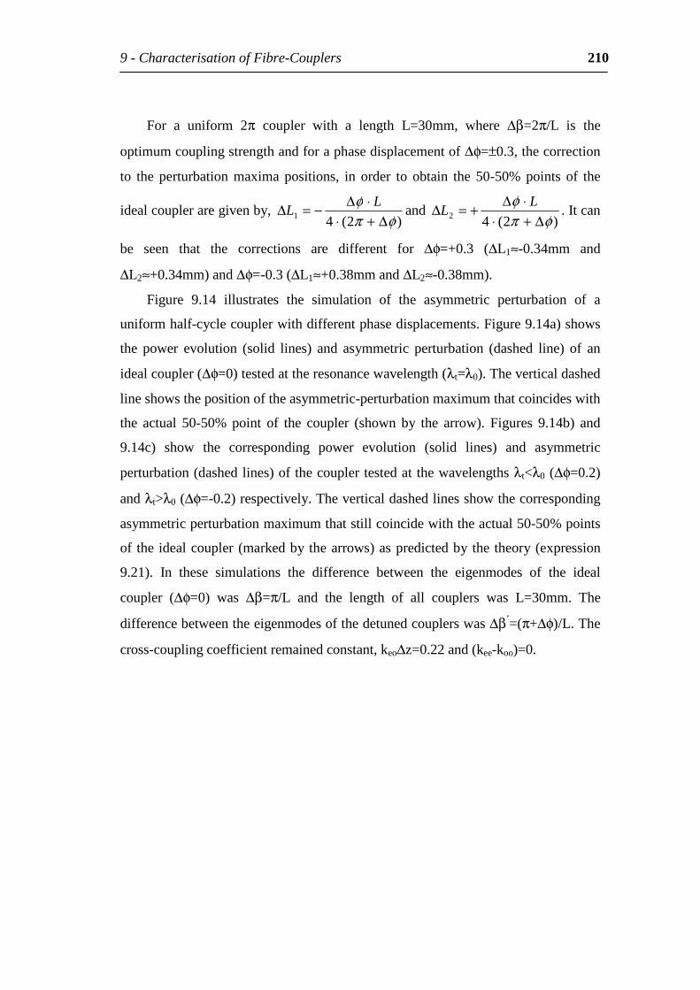
9-CharacterisationofFibre-Couplers 210
For a uniform 2π coupler with a length L=30mm, where ∆β=2π/L is the
optimumcouplingstrengthandforaphasedisplacementof∆φ=±0.3,thecorrection
to the perturbation maxima positions, in order to obtain the 50-50% points of the
idealcoupleraregivenby,)2(41 φπ
φ∆+⋅
⋅∆−=∆ LL and
)2(42 φπφ
∆+⋅⋅∆+=∆ L
L .Itcan
be seen that the corrections are different for ∆φ=+0.3 (∆L1≈-0.34mm and
∆L2≈+0.34mm)and∆φ=-0.3(∆L1≈+0.38mmand∆L2≈-0.38mm).
Figure 9.14 illustrates the simulation of the asymmetric perturbation of a
uniformhalf-cyclecouplerwithdifferentphasedisplacements.Figure9.14a)shows
the power evolution (solid lines) and asymmetric perturbation (dashed line) of an
idealcoupler(∆φ=0)testedattheresonancewavelength(λt=λ0).Theverticaldashed
lineshowsthepositionoftheasymmetric-perturbationmaximumthatcoincideswith
the actual 50-50% point of the coupler (shown by the arrow). Figures 9.14b) and
9.14c) show the corresponding power evolution (solid lines) and asymmetric
perturbation(dashedlines)ofthecouplertestedatthewavelengthsλt<λ0(∆φ=0.2)
andλt>λ0(∆φ=-0.2)respectively.Theverticaldashedlinesshowthecorresponding
asymmetricperturbationmaximumthatstillcoincidewiththeactual50-50%points
of theidealcoupler (markedbythearrows)aspredictedby thetheory(expression
9.21). In these simulations the difference between the eigenmodes of the ideal
coupler (∆φ=0) was ∆β=π/L and the length of all couplers was L=30mm. The
differencebetweentheeigenmodesofthedetunedcouplerswas∆β’=(π+∆φ)/L.The
cross-couplingcoefficientremainedconstant,keo∆z=0.22and(kee-koo)=0.
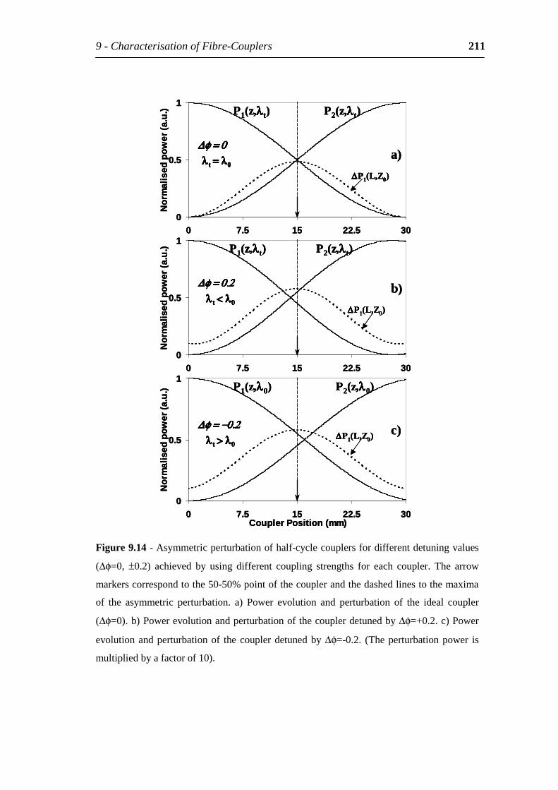
9-CharacterisationofFibre-Couplers 211
0
0.5
1
0 7.5 15 22.5 30
Nor
mal
ised
pow
er(a
.u.)
P1(z,λλλλt) P2(z,λλλλt)
b)∆∆∆∆P1(L,Z0)
∆φ∆φ∆φ∆φ = 0.2= 0.2= 0.2= 0.2λλλλ t < λ< λ< λ< λ0
0
0.5
1
0 7.5 15 22.5 30
Nor
mal
ised
pow
er(a
.u.)
P1(z,λλλλt) P2(z,λλλλt)
a)∆∆∆∆P1(L,Z0)
∆φ∆φ∆φ∆φ = 0= 0= 0= 0λλλλ t = λ= λ= λ= λ0
0
0.5
1
0 7.5 15 22.5 30CouplerPosition(mm)
Nor
mal
ised
pow
er(a
.u.)
P2(z,λλλλ0)P1(z,λλλλ0)
c)∆φ∆φ∆φ∆φ = = = = −−−−0.20.20.20.2λλλλ t > λ> λ> λ> λ0
∆∆∆∆P1(L,Z0)
0
0.5
1
0 7.5 15 22.5 30
Nor
mal
ised
pow
er(a
.u.)
P1(z,λλλλt) P2(z,λλλλt)
b)∆∆∆∆P1(L,Z0)
∆φ∆φ∆φ∆φ = 0.2= 0.2= 0.2= 0.2λλλλ t < λ< λ< λ< λ0
0
0.5
1
0 7.5 15 22.5 30
Nor
mal
ised
pow
er(a
.u.)
P1(z,λλλλt) P2(z,λλλλt)
b)∆∆∆∆P1(L,Z0)
∆φ∆φ∆φ∆φ = 0.2= 0.2= 0.2= 0.2λλλλ t < λ< λ< λ< λ0
∆φ∆φ∆φ∆φ = 0.2= 0.2= 0.2= 0.2λλλλ t < λ< λ< λ< λ0
0
0.5
1
0 7.5 15 22.5 30
Nor
mal
ised
pow
er(a
.u.)
P1(z,λλλλt) P2(z,λλλλt)
a)∆∆∆∆P1(L,Z0)
∆φ∆φ∆φ∆φ = 0= 0= 0= 0λλλλ t = λ= λ= λ= λ0
0
0.5
1
0 7.5 15 22.5 30
Nor
mal
ised
pow
er(a
.u.)
P1(z,λλλλt) P2(z,λλλλt)
a)∆∆∆∆P1(L,Z0)
∆φ∆φ∆φ∆φ = 0= 0= 0= 0λλλλ t = λ= λ= λ= λ0
∆φ∆φ∆φ∆φ = 0= 0= 0= 0λλλλ t = λ= λ= λ= λ0
0
0.5
1
0 7.5 15 22.5 30CouplerPosition(mm)
Nor
mal
ised
pow
er(a
.u.)
P2(z,λλλλ0)P1(z,λλλλ0)
c)∆φ∆φ∆φ∆φ = = = = −−−−0.20.20.20.2λλλλ t > λ> λ> λ> λ0
∆∆∆∆P1(L,Z0)
0
0.5
1
0 7.5 15 22.5 30CouplerPosition(mm)
Nor
mal
ised
pow
er(a
.u.)
P2(z,λλλλ0)P1(z,λλλλ0)
c)∆φ∆φ∆φ∆φ = = = = −−−−0.20.20.20.2λλλλ t > λ> λ> λ> λ0
∆φ∆φ∆φ∆φ = = = = −−−−0.20.20.20.2λλλλ t > λ> λ> λ> λ0
∆∆∆∆P1(L,Z0)
Figure9.14-Asymmetricperturbationofhalf-cyclecouplersfordifferentdetuningvalues
(∆φ=0, ±0.2) achieved by using different coupling strengths for each coupler. The arrow
markerscorrespondtothe50-50%pointofthecouplerandthedashedlinestothemaxima
of the asymmetric perturbation. a) Power evolution and perturbation of the ideal coupler
(∆φ=0).b)Powerevolutionandperturbationofthecouplerdetunedby∆φ=+0.2.c)Power
evolutionandperturbationof thecouplerdetunedby∆φ=-0.2. (Theperturbationpower is
multipliedbyafactorof10).

9-CharacterisationofFibre-Couplers 212
Thecorrectiontothemaximumoftheasymmetricperturbationofahalf-cycle
couplergivenby(9.21)iszeroandthereforeit isamarker tothe50-50%pointof
the half-cycle coupler independently of the coupling strength of the coupler or
equivalently,independentlyofthewavelengthatwhichthecouplerischaracterised
aslongas∆φ=<<π.
Finally,itshouldbestressedthatinthecasethatthecouplerwaististwisted,as
theperturbingelementisscannedalongthecouplerlengthresultsinbothsymmetric
and asymmetric perturbation with mixed results that do not provide any useful
information.
9.4.4 OutputPhasePerturbation
In section 9.3.4 it was shown analytically that for a perfect coupler under pure
asymmetric perturbation (∆φ=0), the phase of the electric field at the output port
with non-null power given by Equation (9.22) is proportional to the power of the
corresponding “ individual” waveguide at the point of the perturbation. Therefore,
the output phase variation maps directly the power evolution along the
corresponding “ individual” waveguide. The phase change due to an asymmetric
perturbationwassimulatedforanidealuniformfull-cyclecoupler(∆φL=0)byusing
expression(9.9).Theasymmetriccross-perturbationcoefficientwaskeo∆z=0.07and
the self-perturbation coefficientswere considered zero (kee=koo=0).The resultsof
thesimulationinFigure9.15showthatthephasevariationθ1oftheelectricfieldat
theoutputof the “ individual” waveguide#1 (solid line) follows indeed closely the
powerevolutionalongthecorresponding“ individual” waveguide.Foranoptimum
cyclecoupler(∆φL=0)withlightlaunchedinport1,thecouplingprofilek(z)canbe
obtainedbymeasuringtheoutputphaseatthesameport.Theoutputphasechanges
canbemeasuredbyusingaphasesensitive(interferometric)technique.
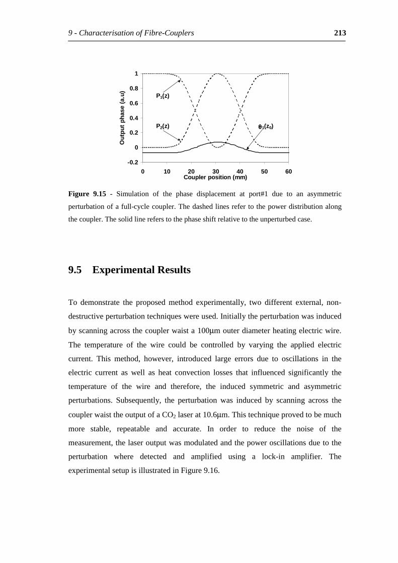
9-CharacterisationofFibre-Couplers 213
-0.2
0
0.2
0.4
0.6
0.8
1
0 10 20 30 40 50 60Couplerposition(mm)
Out
put
phas
e(a
.u)
P1(z)
P2(z) θθθθ1(z0)
Figure 9.15 - Simulation of the phase displacement at port#1 due to an asymmetric
perturbationofafull-cyclecoupler.Thedashedlinesrefertothepowerdistributionalong
thecoupler.Thesolidlinereferstothephaseshiftrelativetotheunperturbedcase.
9.5 ExperimentalResults
To demonstrate the proposed method experimentally, two different external, non-
destructiveperturbationtechniqueswereused.Initiallytheperturbationwasinduced
byscanningacrossthecouplerwaista100µmouterdiameterheatingelectricwire.
The temperature of the wire could be controlled by varying the applied electric
current. This method, however, introduced large errors due to oscillations in the
electric current as well as heat convection losses that influenced significantly the
temperature of the wire and therefore, the induced symmetric and asymmetric
perturbations. Subsequently, the perturbation was induced by scanning across the
couplerwaisttheoutputofaCO2laserat10.6µm.Thistechniqueprovedtobemuch
more stable, repeatable and accurate. In order to reduce the noise of the
measurement,thelaseroutputwasmodulatedandthepoweroscillationsduetothe
perturbation where detected and amplified using a lock-in amplifier. The
experimentalsetupisillustratedinFigure9.16.
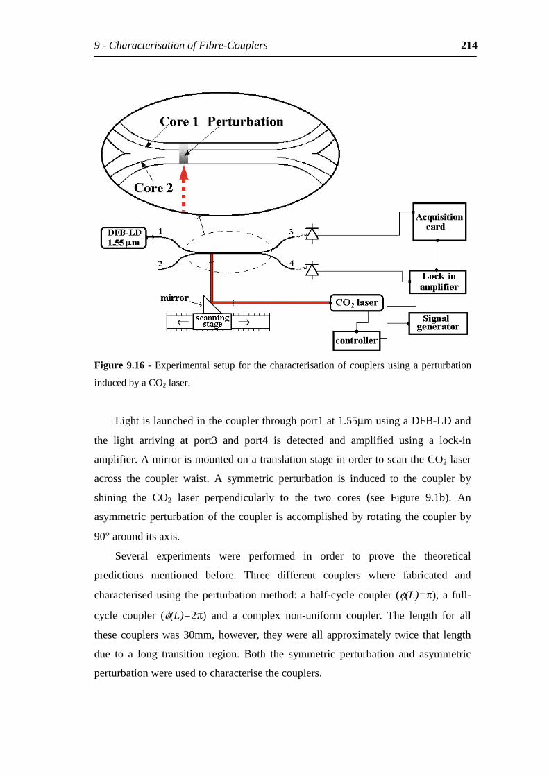
9-CharacterisationofFibre-Couplers 214
Figure9.16 -Experimental setup for thecharacterisationofcouplersusingaperturbation
inducedbyaCO2laser.
Lightislaunchedinthecouplerthroughport1at1.55µmusingaDFB-LDand
the light arriving at port3 and port4 is detected and amplified using a lock-in
amplifier.AmirrorismountedonatranslationstageinordertoscantheCO2laser
across the coupler waist. A symmetric perturbation is induced to the coupler by
shining the CO2 laser perpendicularly to the two cores (see Figure 9.1b). An
asymmetricperturbationof thecoupler isaccomplishedby rotating thecouplerby
90°arounditsaxis.
Several experiments were performed in order to prove the theoretical
predictions mentioned before. Three different couplers where fabricated and
characterisedusing the perturbationmethod: ahalf-cycle coupler (φ(L)=π), a full-
cycle coupler (φ(L)=2π) and a complex non-uniform coupler. The length for all
thesecouplerswas30mm,however, theywere all approximately twice that length
due to a long transition region. Both the symmetric perturbation and asymmetric
perturbationwereusedtocharacterisethecouplers.
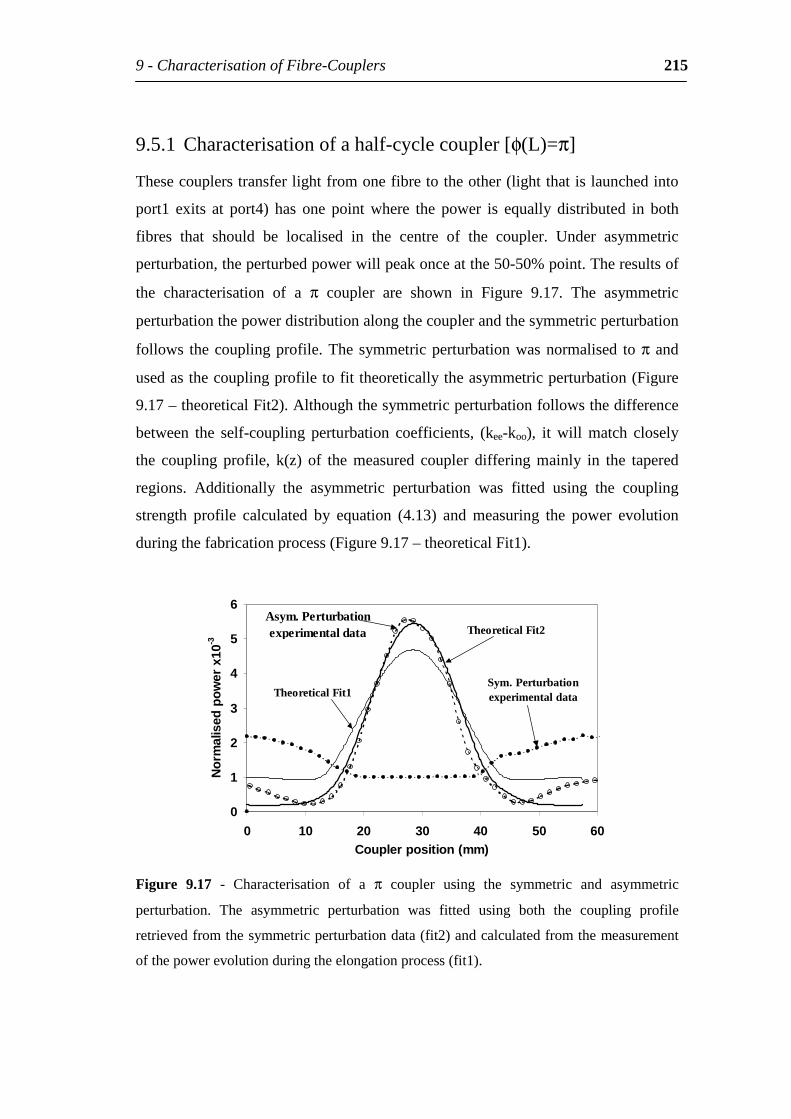
9-CharacterisationofFibre-Couplers 215
9.5.1 Characterisationofahalf-cyclecoupler[φ(L)=π]
Thesecouplerstransferlightfromonefibretotheother(lightthatislaunchedinto
port1 exits at port4) has one point where the power is equally distributed in both
fibres that should be localised in the centre of the coupler. Under asymmetric
perturbation,theperturbedpowerwillpeakonceatthe50-50%point.Theresultsof
the characterisation of a π coupler are shown in Figure 9.17. The asymmetric
perturbationthepowerdistributionalongthecouplerandthesymmetricperturbation
follows thecouplingprofile.Thesymmetricperturbationwasnormalised toπ and
usedasthecouplingprofiletofittheoreticallytheasymmetricperturbation(Figure
9.17–theoreticalFit2).Althoughthesymmetricperturbationfollowsthedifference
between the self-coupling perturbation coefficients, (kee-koo), it will match closely
the coupling profile, k(z) of the measured coupler differing mainly in the tapered
regions. Additionally the asymmetric perturbation was fitted using the coupling
strength profile calculated by equation (4.13) and measuring the power evolution
duringthefabricationprocess(Figure9.17–theoreticalFit1).
0
1
2
3
4
5
6
0 10 20 30 40 50 60Couplerposition(mm)
Nor
mal
ised
pow
erx
10-3
Asym.Perturbationexperimentaldata TheoreticalFit2
Sym.PerturbationexperimentaldataTheoreticalFit1
Figure 9.17 - Characterisation of a π coupler using the symmetric and asymmetric
perturbation. The asymmetric perturbation was fitted using both the coupling profile
retrievedfromthesymmetricperturbationdata(fit2)andcalculatedfromthemeasurement
ofthepowerevolutionduringtheelongationprocess(fit1).
9-CharacterisationofFibre-Couplers 216
From this Figure it was realised that the experimental coupling strength obtained
using the symmetric perturbation of the coupler was better suited than the one
calculated from (4.13), to fit the asymmetric perturbation data. This is due to
equation (4.13)beingan approximation to the casewhere the sizeof the flame is
infinitesimalandinrealityitisapproximately4mmwideresultinginanactualwaist
radiusdifferingfromtheburnertravel.
Insections9.3.3itwasmentionedthatthemaximumofthepowerchange,due
to an asymmetric perturbation, is a marker for the 50-50% points of the coupler
independentlyofthesmallphasedetuningofthecoupler(eitherduetostraininthe
mountingof thecoupleror thecharacterisation atawavelengthdifferent from the
coupler resonance wavelength). This information is very useful since the 50-50%
pointsofhalf-cyclecouplerscanbealwaysobtainedwithusinganormallaserdiode
tocharacterisethecouplerandwithouttheneedofatunablelasersettothecoupler
exact resonance wavelength. In Figure 9.18 experimental results of the
characterisation of a half-cycle coupler at different wavelengths are shown. A
tunablelaserwasusedtolaunchlightinthecouplerport#1insteadoftheDFB-LD
as shown in experimental setup (Figure 9.14). Three different test wavelengths
where used: λ0=1510nm, λ1=1550nm (coupler resonance wavelength) and
λ2=1590nm. The power of the CO2 laser was the same for all the experiments
(100mWthrougha2mmpinhole).
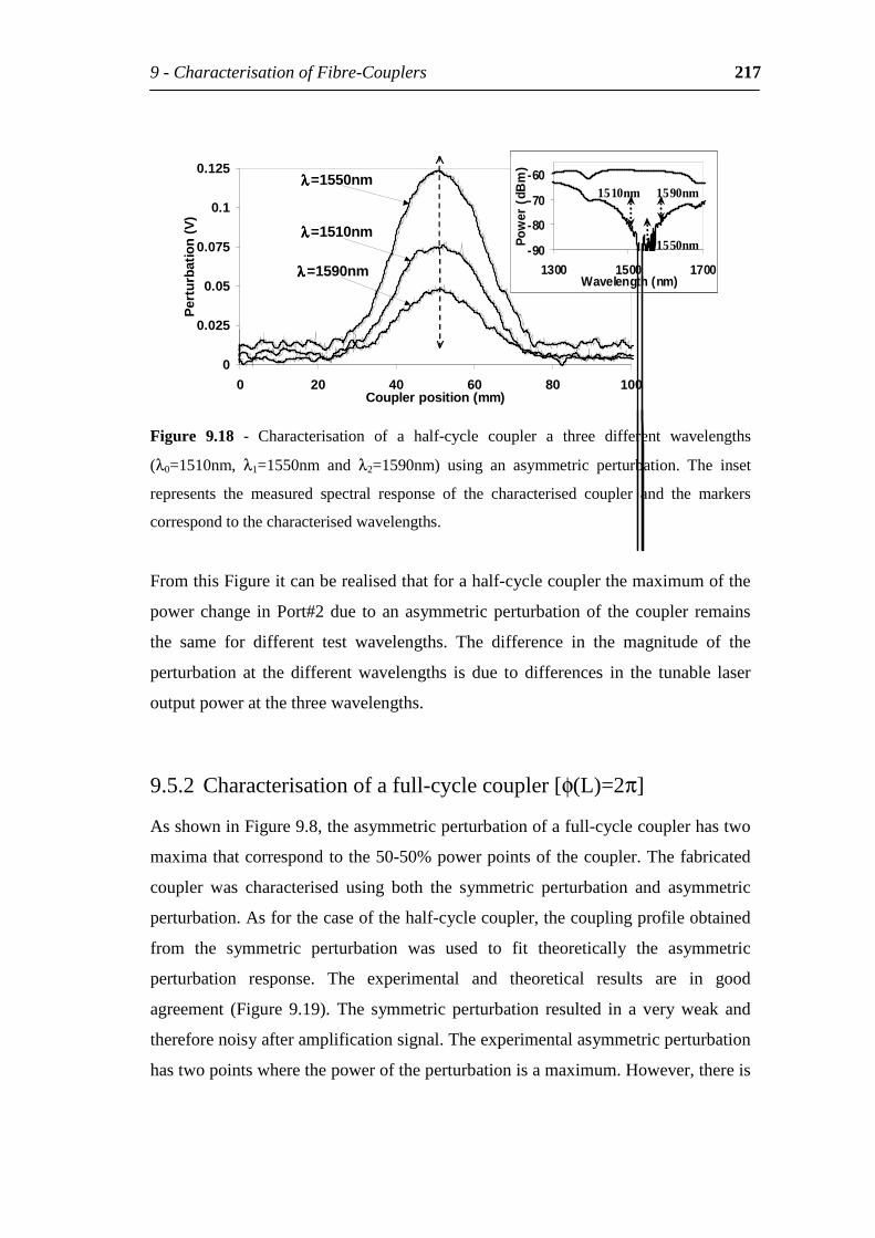
9-CharacterisationofFibre-Couplers 217
0
0.025
0.05
0.075
0.1
0.125
0 20 40 60 80 100Couplerposition(mm)
Per
turb
atio
n(V
)λλλλ=1550nm
λλλλ=1510nm
λλλλ=1590nm-90
-80
-70
-60
1300 1500 1700Wavelength(nm)
Pow
er(
dBm
)
1590nm1510nm
1550nm
0
0.025
0.05
0.075
0.1
0.125
0 20 40 60 80 100Couplerposition(mm)
Per
turb
atio
n(V
)λλλλ=1550nm
λλλλ=1510nm
λλλλ=1590nm-90
-80
-70
-60
1300 1500 1700Wavelength(nm)
Pow
er(
dBm
)
1590nm1510nm
1550nm
Figure 9.18 - Characterisation of a half-cycle coupler a three different wavelengths
(λ0=1510nm, λ1=1550nm and λ2=1590nm) using an asymmetric perturbation. The inset
represents the measured spectral response of the characterised coupler and the markers
correspondtothecharacterisedwavelengths.
FromthisFigureitcanberealisedthatforahalf-cyclecouplerthemaximumofthe
powerchange inPort#2due toanasymmetricperturbationof thecoupler remains
the same for different test wavelengths. The difference in the magnitude of the
perturbation at the different wavelengths is due to differences in the tunable laser
outputpoweratthethreewavelengths.
9.5.2 Characterisationofafull-cyclecoupler[φ(L)=2π]
AsshowninFigure9.8,theasymmetricperturbationofafull-cyclecouplerhastwo
maximathatcorrespondtothe50-50%powerpointsofthecoupler.Thefabricated
coupler was characterised using both the symmetric perturbation and asymmetric
perturbation.Asforthecaseofthehalf-cyclecoupler,thecouplingprofileobtained
from the symmetric perturbation was used to fit theoretically the asymmetric
perturbation response. The experimental and theoretical results are in good
agreement (Figure 9.19). The symmetric perturbation resulted in a very weak and
thereforenoisyafteramplificationsignal.Theexperimentalasymmetricperturbation
hastwopointswherethepoweroftheperturbationisamaximum.However,thereis
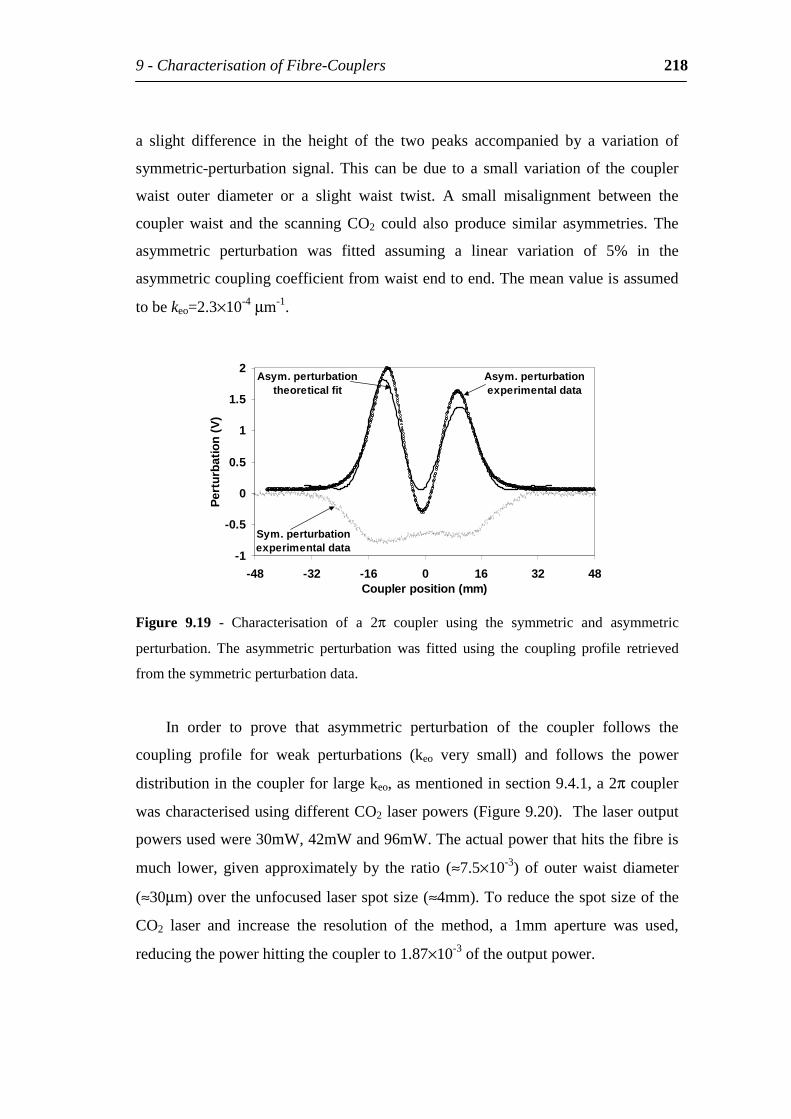
9-CharacterisationofFibre-Couplers 218
a slight difference in the height of the two peaks accompanied by a variation of
symmetric-perturbation signal.This canbedue to a small variationof the coupler
waist outer diameter or a slight waist twist. A small misalignment between the
coupler waist and the scanning CO2 could also produce similar asymmetries. The
asymmetric perturbation was fitted assuming a linear variation of 5% in the
asymmetriccouplingcoefficientfromwaistendtoend.Themeanvalueisassumed
tobekeo=2.3×10⁻⁴µm-1.
-1
-0.5
0
0.5
1
1.5
2
-48 -32 -16 0 16 32 48Couplerposition(mm)
Per
turb
atio
n(V
)
Sym.perturbationexperimentaldata
Asym.perturbationexperimentaldata
Asym.perturbationtheoreticalfit
Figure 9.19 - Characterisation of a 2π coupler using the symmetric and asymmetric
perturbation. The asymmetric perturbation was fitted using the coupling profile retrieved
fromthesymmetricperturbationdata.
In order to prove that asymmetric perturbation of the coupler follows the
coupling profile for weak perturbations (keo very small) and follows the power
distributioninthecouplerforlargekeo,asmentionedinsection9.4.1,a2πcoupler
wascharacterisedusingdifferentCO2laserpowers(Figure9.20).Thelaseroutput
powersusedwere30mW,42mWand96mW.Theactualpowerthathitsthefibreis
much lower, given approximately by the ratio (≈7.5×10⁻³) of outer waist diameter
(≈30µm)overtheunfocusedlaserspotsize(≈4mm).Toreducethespotsizeofthe
CO2 laser and increase the resolution of the method, a 1mm aperture was used,
reducingthepowerhittingthecouplerto1.87×10-3oftheoutputpower.
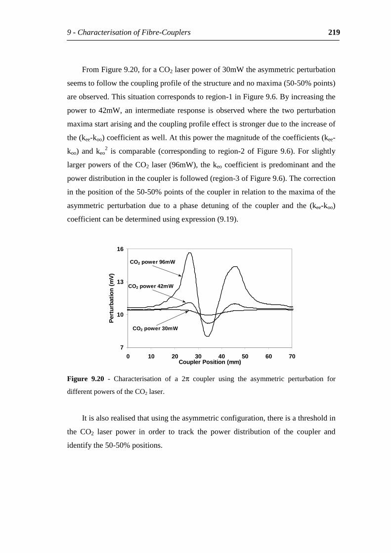
9-CharacterisationofFibre-Couplers 219
FromFigure9.20,foraCO2laserpowerof30mWtheasymmetricperturbation
seemstofollowthecouplingprofileofthestructureandnomaxima(50-50%points)
areobserved.Thissituationcorrespondstoregion-1inFigure9.6.Byincreasingthe
power to42mW,an intermediate response isobservedwhere the twoperturbation
maximastartarisingandthecouplingprofileeffectisstrongerduetotheincreaseof
the(kee-koo)coefficientaswell.Atthispowerthemagnitudeofthecoefficients(kee-
koo) andkeo2 is comparable (corresponding to region-2ofFigure9.6).For slightly
largerpowersof theCO2 laser(96mW),thekeocoefficient ispredominantandthe
powerdistributioninthecouplerisfollowed(region-3ofFigure9.6).Thecorrection
inthepositionofthe50-50%pointsofthecouplerinrelationtothemaximaofthe
asymmetric perturbation due to a phase detuning of the coupler and the (kee-koo)
coefficientcanbedeterminedusingexpression(9.19).
7
10
13
16
0 10 20 30 40 50 60 70CouplerPosition(mm)
Per
turb
atio
n(m
V)
CO2power42mW
CO2power96mW
CO2power30mW
Figure 9.20 - Characterisation of a 2π coupler using the asymmetric perturbation for
differentpowersoftheCO2laser.
Itisalsorealisedthatusingtheasymmetricconfiguration,thereisathresholdin
the CO2 laser power in order to track the power distribution of the coupler and
identifythe50-50%positions.
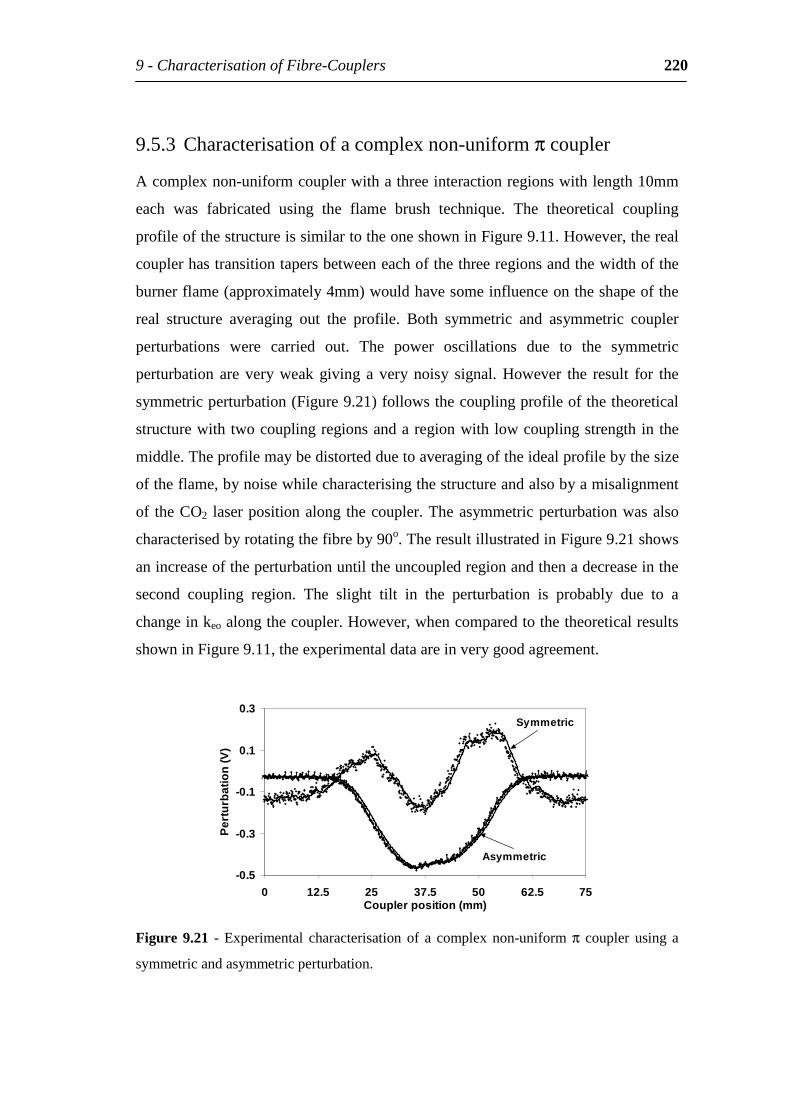
9-CharacterisationofFibre-Couplers 220
9.5.3 Characterisationofacomplexnon-uniformπcoupler
Acomplexnon-uniformcouplerwithathreeinteractionregionswithlength10mm
each was fabricated using the flame brush technique. The theoretical coupling
profileofthestructureissimilartotheoneshowninFigure9.11.However,thereal
couplerhastransitiontapersbetweeneachofthethreeregionsandthewidthofthe
burnerflame(approximately4mm)wouldhavesomeinfluenceontheshapeofthe
real structure averaging out the profile. Both symmetric and asymmetric coupler
perturbations were carried out. The power oscillations due to the symmetric
perturbation are very weak giving a very noisy signal. However the result for the
symmetricperturbation(Figure9.21)followsthecouplingprofileofthetheoretical
structurewithtwocouplingregionsandaregionwithlowcouplingstrengthinthe
middle.Theprofilemaybedistortedduetoaveragingoftheidealprofilebythesize
oftheflame,bynoisewhilecharacterisingthestructureandalsobyamisalignment
of theCO2 laserpositionalong thecoupler.Theasymmetricperturbationwasalso
characterisedbyrotatingthefibreby90o.TheresultillustratedinFigure9.21shows
anincreaseoftheperturbationuntiltheuncoupledregionandthenadecreaseinthe
second coupling region. The slight tilt in the perturbation is probably due to a
changeinkeoalongthecoupler.However,whencomparedtothetheoreticalresults
showninFigure9.11,theexperimentaldataareinverygoodagreement.
-0.5
-0.3
-0.1
0.1
0.3
0 12.5 25 37.5 50 62.5 75Couplerposition(mm)
Per
turb
atio
n(V
)
Symmetric
Asymmetric
Figure 9.21 - Experimental characterisation of a complexnon-uniformπ coupler using a
symmetricandasymmetricperturbation.
9-CharacterisationofFibre-Couplers 221
It is thereforeconcludedthatboththeasymmetricandsymmetricperturbation
configurations can be used to identify the central region of the non-uniform
couplers. This method can be employed when writing gratings in non-uniform
couplers so that thegrating iswritten in the correctposition, avoiding the tapered
regionsthatdegradetheperformanceofthesedevicesasdiscussedinchapter8.
9.6 Summary
Afulldescriptionofamethodofnon-destructivelycharacterisinguniformandnon-
uniform fibre couplerswasdescribed.Themethodconsists inperturbing locally a
fibrecouplerusingaCO2laserradiationorotherradiationwithapenetrationlength
closetothecouplerdiameter.Byinducingasymmetricperturbationwithrespectto
the two lowest order waist eigenmodes, useful information about the taper profile
and uniformity of the coupler waist can be obtained. By inducing an asymmetric
perturbation,ontheotherhand,thepowerevolutionalongtheentirecouplingregion
canbefollowed.Additional informationmaybeobtainedbymeasuring theoutput
electricfieldphaseinthecaseoftheasymmetricandsymmetricperturbations.The
method can used for the optimisation of add/drop multiplexers based on different
couplerstructureswithinscribedgratings.Itcanalsobeusedinindustrialfacilities
fortheidentificationoferrorsandoptimisationofthefabricationprocedureoffibre
couplers (powersplittersorWDMcouplers)by thesuitablecharacterisationof the
devices. This method was initially developed with the purpose of optimising the
performance of the add-drop multiplexers discussed in chapter 8. Experimentally,
the CO2 laser was integrated with the grating writing system in order to first
characterise the couplers and subsequently inscribe the gratings at the correct
positioninordertooptimisetheadd-dropperformance.However,hydrogenloading
canchange thecoupler resonancewavelengthbymore than100nmandwhen it is
characterised themeasured50-50%positions shouldbe corrected.For an accurate
correctionof thesepositions, theknowledgeof theexactcouplerprofile shouldbe
9-CharacterisationofFibre-Couplers 222
known.Anotherdrawbackistheacceleratedhydrogenout-diffusingduetotheheat
generatedbytheincidentCO2radiationthatinducesfurtherchangestothecoupler
andmakingthemeasurementlessreliable.Therefore,ideally,thecouplersshouldbe
characterisedbeforetheprocessofincreasingitsphotosensitivity.
10
Summary
Theincreasingdemandforhigh-speedcommunicationshasledtothewidespreadof
WDMLAN,METRO,andlong-haulnetworks.InLANandMETROinparticular,
duetothenumberofopticalnodesinvolved,cost-effectivesolutionsareimportant
toassurecompetitive services.Keycomponentsof theseopticalnetworks include;
equalised EDFA that amplify uniformly the optical signals, add-drop multiplexers
thatareusedtorouteselectedchannelstodifferentlocationsatstrategicpointsalong
thenetwork, and fibre couplers that areused to monitor thenetwork, split optical
signals or provide pump/signal discriminators when launching into EDFAs. The
contentofthisthesiswasaimedmainlyatthesetwotechnologies,essentialforthe
deploymentofWDMnetworks.
10–Summary 225
10.1 EDFAgainequalisation
Design of ideal filters for EDFA gain equalisation can reduce the number of
amplifiers needed in the optical network by: compensating for insertion losses,
increasing theamplifiergain,and increasing theamplifierbandwidth. In thiswork
theoreticaldesignandnumericalmodellingofidealfiltersfortheequalisationofthe
EDFAgainspectrumwerestudied,givingamethodofdetermining the ideal filter
shapesandoptimumpositionintheamplifierinordertoobtainthebestperformance
whileequalisingtheEDFAgainspectrum.Thesefiltersareoriginallydeterminedas
an ideal wavelength-dependent background loss and are integrated in one or two
filters, placed within the EDFA. The performance of both these configurations is
compared.Furthermore,theperformanceoffilters,designedtobeplacedbothinside
andoutsidetheEDFA,wasalsoconsideredandcompared.Itwasalsodemonstrated
thatfollowingourdesignprocedure,thegain-flatteningfiltercouldberedesignedto
compensateforitsown,aswellas,otherdevices’ insertionloss.Withthismethodit
wasshownthatfilterswithinsertionlossupto8dBcouldbeusedwithoutpenaltyin
the amplifier gain. Such filter designs can have huge impact on the number of
amplifiersusedinalinkandthesystempowerbudget.
The saturation of the EDFA varies with the several parameters including the
input signal. Dynamic equalisation is needed to adjust the filter shape in order to
equalise the EDFA gain spectrum for different saturations. An alternative AO
tunable filter design was demonstrated as a means of achieving dynamic gain
equalisation with reduced tuning parameters comparing to previous design. The
controlofthewaistradiusofafibre-taperwasdemonstratedtobeanewmeansof
tailoring the loss spectrum of AO filters. Tunable filters can be designed to have
faster reshaping algorithms and ideal spectral shapes using the theoretical method
fordesigningidealfilters,inordertoequalisetheEDFAgainspectrumwiththebest
performance.
10–Summary 226
10.2 Add-dropmultiplexers
The ability to route selected wavelength channels at different locations along the
opticallinkisessentialforthedesignofefficientWDMnetworks.Thedemandfor
cheapadd-dropmultiplexerstoperformtheseoperationshasledtotheinvestigation
ofcompactall-fibreconfigurationsbasedonBragggratingsinscribedinthewaistof
fibre couplers. Optimisation parameters of three different designs are discussed in
this work with emphasis on a novel device based on a non-uniform half-cycle
coupler with a grating inscribed in its waist. This device is demonstrated
experimentallytopotentiallysatisfyDWDMstandardswhenfullyoptimised.
Thesuitablecharacterisationoffibrecouplersisimportantforthedetermination
ofthecorrectposition,wherethegrating,shouldbeinscribed,withinthecoupler.A
novel non-destructive coupler characterisation technique was developed in this
work.Allthreeadd-dropconfigurationsanalysedinthisworkcanbenefitfromthis
techniquebothbydeterminationofthecouplerstrengthprofileandpowerevolution
andbyusing themethodasanassessment tool tooptimise thecoupler fabrication
procedure.Finally,onitsownthistechniqueisanimportanttooltoassesserrorsin
couplerfabricationprocessesingeneral.
10.3 FutureWork
The work on the design of ideal filters for EDFA gain equalisation could be
followedbyexperimentalverification.Thiswould involve themeasurementof the
EDFparametersandthedesignoffiltersforthegivenamplifierusingshort-aswell
as long-period grating technology or AO technology. The impact of the EDFA
inhomogeneousbroadeningontheperformanceofthesefilterscouldbeaddressedas
well.
Following the work on the add-drop multiplexer it will be interesting to
integratethecouplercharacterisationtechniquewithagoodqualitygratingwriting
setupinordertohavefullcontrolonthepositionthegratingsareplacedwithinthe

10–Summary 227
couplers. Optimisation of the fabrication of non-uniform couplers to increase the
centrallengthandhavebettercontrolonthetaperedregionshapecouldbeachieved
byfabricatingthecouplersusingafocusedCO2laserbeam.
APPENDIXA
Add-droprequirements
Thetablepresentedinthisappendixrefertochapters3and8.Itgivesvaluesforthe
performancerequirementsofadd-dropmultiplexerdevices.
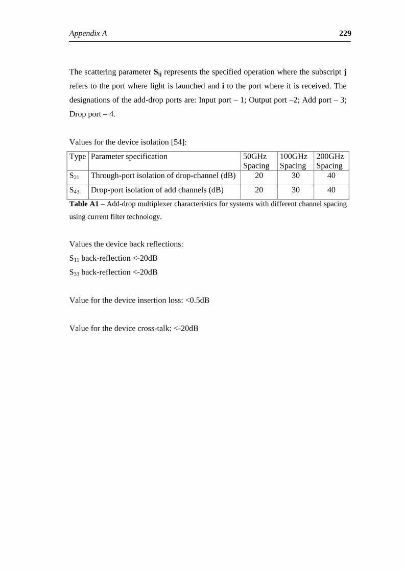
AppendixA 229
ThescatteringparameterSijrepresentsthespecifiedoperationwherethesubscriptj
referstotheportwherelightislaunchedanditotheportwhereitisreceived.The
designationsoftheadd-dropportsare:Inputport–1;Outputport–2;Addport–3;
Dropport–4.
Valuesforthedeviceisolation[54]:
Type Parameterspecification 50GHzSpacing
100GHzSpacing
200GHzSpacing
S21 Through-portisolationofdrop-channel(dB) 20 30 40
S43 Drop-portisolationofaddchannels(dB) 20 30 40
TableA1–Add-dropmultiplexercharacteristicsforsystemswithdifferentchannelspacing
usingcurrentfiltertechnology.
Valuesthedevicebackreflections:
S11back-reflection<-20dB
S33back-reflection<-20dB
Valueforthedeviceinsertionloss:<0.5dB
Valueforthedevicecross-talk:<-20dB
AppendixB
Fielddistributions
Thefiguresillustratedinthisappendixrefertochapter6.
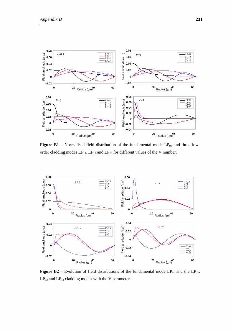
AppendixB 231
-0.02
0
0.02
0.04
0.06
0.08
0 20 40 60Radius(µm)
Fie
lda
mpl
itude
(a.
u.) LP01
LP11LP12LP13
V=0.1
-0.02
0
0.02
0.04
0.06
0.08
0 20 40 60Radius(µm)
Fiel
dam
plitu
de(a
.u.) LP01
LP11LP12LP13
V=1
-0.02
0
0.02
0.04
0.06
0.08
0 20 40 60Radius(µm)
Fiel
dam
plitu
de(a
.u.) LP01
LP11LP12LP13
V=2
-0.04
-0.02
0
0.02
0.04
0.06
0.08
0 20 40 60Radius(µm)
Fiel
dam
plitu
de(a
.u.) LP01
LP11LP12LP13
V=3
Figure B1 – Normalised field distribution of the fundamental mode LP01 and three low-
ordercladdingmodesLP11,LP12andLP13fordifferentvaluesoftheVnumber.
0
0.02
0.04
0.06
0.08
0 20 40 60Radius(µm)
Fiel
dam
plitu
de(a
.u.) V=0.1
V=1V=2V=3
LP01
0
0.02
0.04
0.06
0 20 40 60Radius(µm)
Fiel
dam
plitu
de(a
.u.) V=0.1
V=1V=2V=3
LP11
-0.02
0
0.02
0.04
0 20 40 60Radius(µm)
Fiel
dam
plitu
de(a
.u.) V=0.1
V=1V=2V=3
LP12
-0.04
-0.02
0
0.02
0.04
0 20 40 60Radius(µm)
Fiel
dam
plitu
de(a
.u.)
V=0.1V=1V=2V=3
LP13
FigureB2–Evolutionof fielddistributionsof the fundamentalmodeLP01 and theLP11,
LP12andLP13claddingmodeswiththeVparameter.
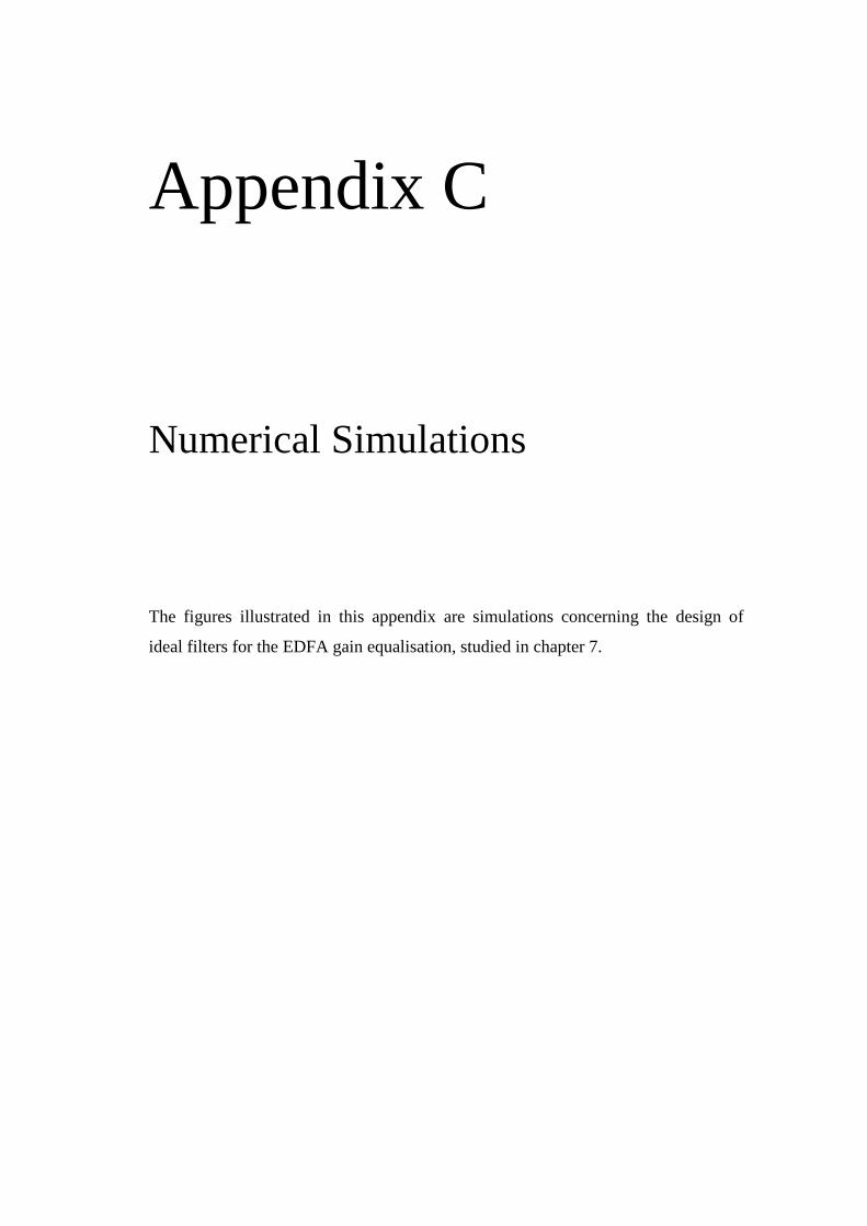
AppendixC
NumericalSimulations
The figures illustrated in this appendix are simulations concerning the design of
idealfiltersfortheEDFAgainequalisation,studiedinchapter7.
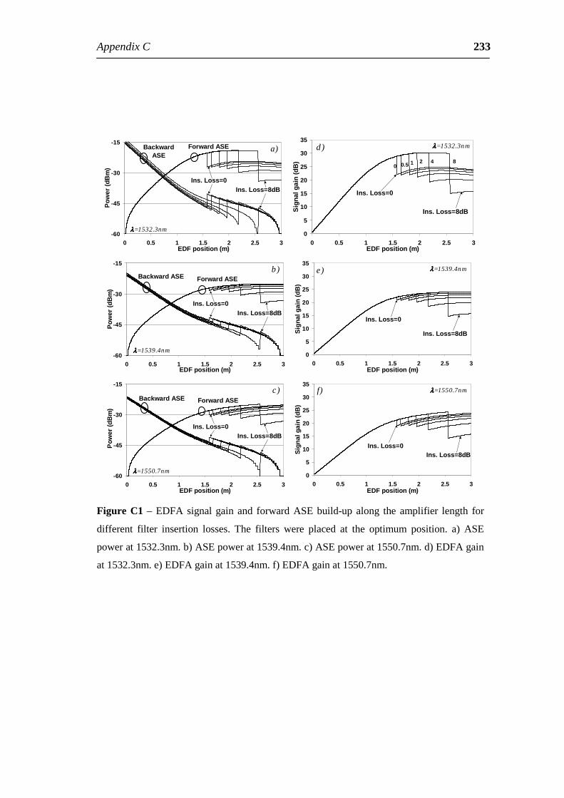
AppendixC 233
-60
-45
-30
-15
0 0.5 1 1.5 2 2.5 3EDFposition(m)
Pow
er(d
Bm
)
a)
λλλλ=1532.3nm
ForwardASEBackwardASE
Ins.Loss=8dBIns.Loss=0
0
5
10
15
20
25
30
35
0 0.5 1 1.5 2 2.5 3EDFposition(m)
Sig
nalg
ain
(dB
)
d)
Ins.Loss=8dB
Ins.Loss=0
0.5 1 2 4 80
λλλλ=1532.3nm
-60
-45
-30
-15
0 0.5 1 1.5 2 2.5 3EDFposition(m)
Pow
er(d
Bm
)
b)
λλλλ=1539.4nm
ForwardASEBackwardASE
Ins.Loss=8dBIns.Loss=0
0
5
10
15
20
25
30
35
0 0.5 1 1.5 2 2.5 3EDFposition(m)
Sig
nalg
ain
(dB
)
e)
Ins.Loss=8dB
Ins.Loss=0
λλλλ=1539.4nm
-60
-45
-30
-15
0 0.5 1 1.5 2 2.5 3EDFposition(m)
Pow
er(d
Bm
)
c)
λλλλ=1550.7nm
ForwardASEBackwardASE
Ins.Loss=8dBIns.Loss=0
0
5
10
15
20
25
30
35
0 0.5 1 1.5 2 2.5 3EDFposition(m)
Sig
nalg
ain
(dB
)
f)
Ins.Loss=8dBIns.Loss=0
λλλλ=1550.7nm
FigureC1–EDFAsignalgain and forwardASEbuild-upalong the amplifier length for
different filter insertion losses. The filters were placed at the optimum position. a) ASE
powerat1532.3nm.b)ASEpowerat1539.4nm.c)ASEpowerat1550.7nm.d)EDFAgain
at1532.3nm.e)EDFAgainat1539.4nm.f)EDFAgainat1550.7nm.
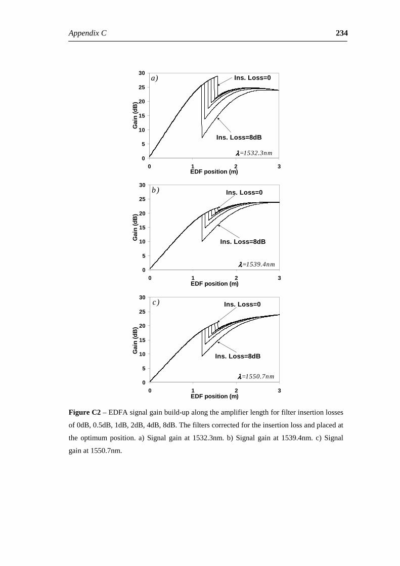
AppendixC 234
0
5
10
15
20
25
30
0 1 2 3EDFposition(m)
Gai
n(d
B)
a)
Ins.Loss=8dB
Ins.Loss=0
λλλλ=1532.3nm
0
5
10
15
20
25
30
0 1 2 3EDFposition(m)
Gai
n(d
B)
λλλλ=1539.4nm
b) Ins.Loss=0
Ins.Loss=8dB
0
5
10
15
20
25
30
0 1 2 3EDFposition(m)
Gai
n(d
B)
λλλλ=1550.7nm
c)
Ins.Loss=8dB
Ins.Loss=0
FigureC2–EDFAsignalgainbuild-upalongtheamplifierlengthforfilterinsertionlosses
of0dB,0.5dB,1dB,2dB,4dB,8dB.Thefilterscorrectedfortheinsertionlossandplacedat
the optimum position. a) Signal gain at 1532.3nm. b) Signal gain at 1539.4nm. c) Signal
gainat1550.7nm.
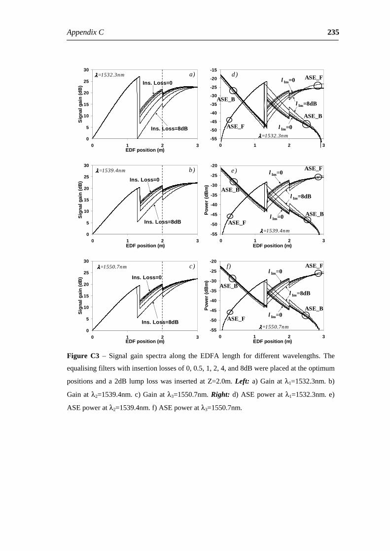
AppendixC 235
0
5
10
15
20
25
30
0 1 2 3EDFposition(m)
Sig
nalg
ain
(dB
)a)
Ins.Loss=8dB
Ins.Loss=0λλλλ=1532.3nm
-55
-50
-45
-40
-35
-30
-25
-20
-15
0 1 2 3
d)
l Ins=8dB
l Ins=0
λλλλ=1532.3nm
l Ins=0
ASE_F
ASE_B
ASE_B
ASE_F
0
5
10
15
20
25
30
0 1 2 3EDFposition(m)
Sig
nalg
ain
(dB
)
b)
Ins.Loss=8dB
Ins.Loss=0
λλλλ=1539.4nm
-55
-50
-45
-40
-35
-30
-25
-20
0 1 2 3EDFposition(m)
Pow
er(d
Bm
)
e)
l Ins=8dB
l Ins=0
λλλλ=1539.4nm
l Ins=0
ASE_F
ASE_B
ASE_B
ASE_F
0
5
10
15
20
25
30
0 1 2 3EDFposition(m)
Sig
nalg
ain
(dB
)
c)
Ins.Loss=8dB
Ins.Loss=0
λλλλ=1550.7nm
-55
-50
-45
-40
-35
-30
-25
-20
0 1 2 3EDFposition(m)
Pow
er(d
Bm
)
f)
l Ins=8dB
l Ins=0
λλλλ=1550.7nm
l Ins=0
ASE_F
ASE_B
ASE_B
ASE_F
Figure C3 – Signal gain spectra along the EDFA length for different wavelengths. The
equalisingfilterswithinsertionlossesof0,0.5,1,2,4,and8dBwereplacedattheoptimum
positionsanda2dB lump losswas insertedatZ=2.0m.Left: a)Gainatλ1=1532.3nm.b)
Gainatλ2=1539.4nm.c)Gainatλ3=1550.7nm.Right:d)ASEpoweratλ1=1532.3nm.e)
ASEpoweratλ2=1539.4nm.f)ASEpoweratλ3=1550.7nm.
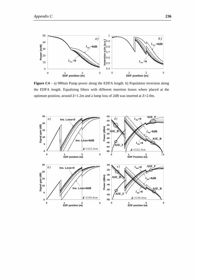
AppendixC 236
0
10
20
30
40
50
0 1 2 3EDFposition(m)
Po
wer
(m
W)
a)
l Ins =8dB
l Ins =0
0.4
0.5
0.6
0.7
0.8
0.9
1
0 1 2 3EDFposition(m)
Inve
rsio
nn
2/n
t(a.
u.) b)
l Ins =8dB
l Ins =0
FigureC4–a)980nmPumppoweralongtheEDFAlength.b)Populationinversionalong
the EDFA length. Equalising filters with different insertion losses where placed at the
optimumposition,aroundZ=1.2mandalumplossof2dBwasinsertedatZ=2.0m.
0
5
10
15
20
25
0 1 2 3EDFposition(m)
Sig
nalg
ain
(dB
)
a)
Ins.Loss=8dB
Ins.Loss=0
λλλλ=1532.3nm-55
-50
-45
-40
-35
-30
-25
-20
-15
0 1 2 3EDFPosition(m)
Pow
er(d
Bm
)
d)
l Ins=8dB
l Ins=0
λλλλ=1532.3nm
l Ins=0
ASE_F
ASE_B
ASE_B
ASE_F
0
5
10
15
20
25
0 1 2 3EDFposition(m)
Sig
nalg
ain
(dB
)
b)
Ins.Loss=8dB
Ins.Loss=0
λλλλ=1539.4nm-55
-50
-45
-40
-35
-30
-25
-20
0 1 2 3EDFposition(m)
Pow
er(d
Bm
)
e)
l Ins=8dB
l Ins=0
λλλλ=1539.4nm
l Ins=0
ASE_F
ASE_B
ASE_B
ASE_F
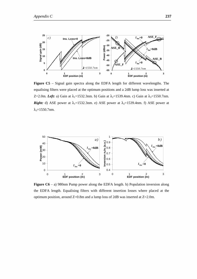
AppendixC 237
0
5
10
15
20
25
0 1 2 3EDFposition(m)
Sig
nalg
ain
(dB
)c)
Ins.Loss=8dB
Ins.Loss=0
λλλλ=1550.7nm-55
-50
-45
-40
-35
-30
-25
-20
0 1 2 3EDFposition(m)
Pow
er(d
Bm
)
f)
l Ins=8dB
l Ins=0
λλλλ=1550.7nm
l Ins=0
ASE_F
ASE_B
ASE_B
ASE_F
Figure C5 – Signal gain spectra along the EDFA length for different wavelengths. The
equalisingfilterswereplacedattheoptimumpositionsanda2dBlumplosswasinsertedat
Z=2.0m.Left:a)Gainatλ1=1532.3nm.b)Gainatλ2=1539.4nm.c)Gainatλ3=1550.7nm.
Right: d) ASE power at λ1=1532.3nm. e) ASE power at λ2=1539.4nm. f) ASE power at
λ3=1550.7nm.
0
10
20
30
40
50
0 1 2 3EDFposition(m)
Po
wer
(m
W)
a)
l Ins =8dB
l Ins =00.4
0.5
0.6
0.7
0.8
0.9
1
0 1 2 3EDFposition(m)
Inve
rsio
nn
2/n
t(a.
u.) b)
l Ins =8dB
l Ins =0
FigureC6–a)980nmPumppoweralongtheEDFAlength.b)Populationinversionalong
the EDFA length. Equalising filters with different insertion losses where placed at the
optimumposition,aroundZ=0.8mandalumplossof2dBwasinsertedatZ=2.0m.
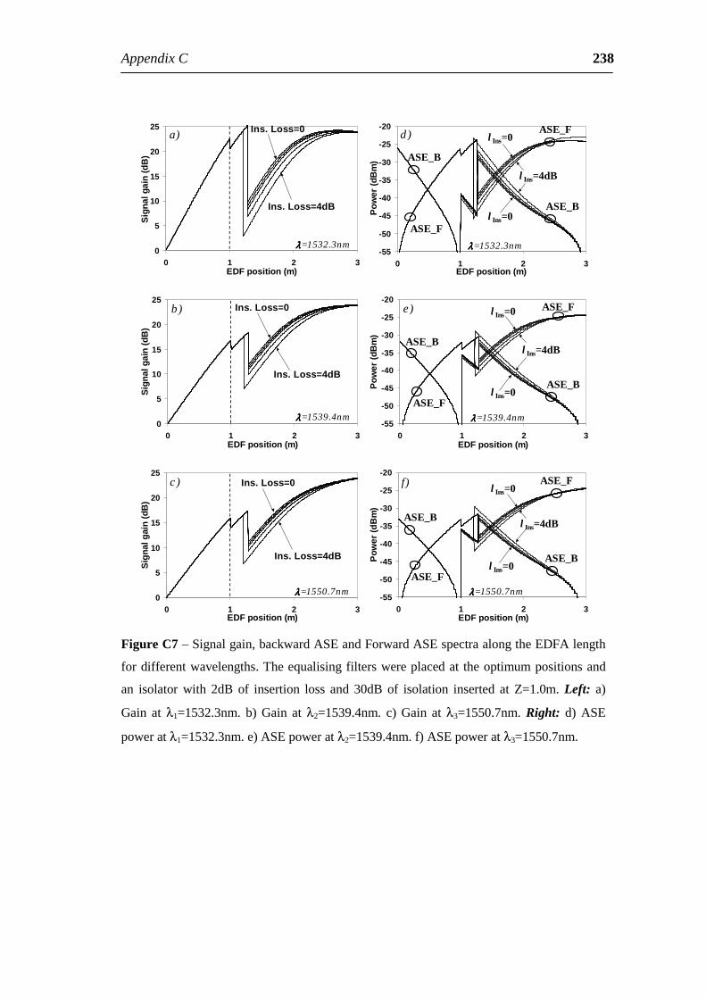
AppendixC 238
0
5
10
15
20
25
0 1 2 3EDFposition(m)
Sig
nalg
ain
(dB
)a)
Ins.Loss=4dB
Ins.Loss=0
λλλλ=1532.3nm-55
-50
-45
-40
-35
-30
-25
-20
0 1 2 3EDFposition(m)
Pow
er(d
Bm
)
d)
l Ins=4dB
l Ins=0
λλλλ=1532.3nm
l Ins=0
ASE_F
ASE_B
ASE_B
ASE_F
0
5
10
15
20
25
0 1 2 3EDFposition(m)
Sig
nalg
ain
(dB
)
b)
Ins.Loss=4dB
Ins.Loss=0
λλλλ=1539.4nm-55
-50
-45
-40
-35
-30
-25
-20
0 1 2 3EDFposition(m)
Pow
er(d
Bm
)
e)
l Ins=4dB
l Ins=0
λλλλ=1539.4nm
l Ins=0
ASE_F
ASE_B
ASE_B
ASE_F
0
5
10
15
20
25
0 1 2 3EDFposition(m)
Sig
nalg
ain
(dB
)
c)
Ins.Loss=4dB
Ins.Loss=0
λλλλ=1550.7nm-55
-50
-45
-40
-35
-30
-25
-20
0 1 2 3EDFposition(m)
Pow
er(d
Bm
)
f)
l Ins=4dB
l Ins=0
λλλλ=1550.7nm
l Ins=0
ASE_F
ASE_B
ASE_B
ASE_F
FigureC7–Signalgain,backwardASEandForwardASEspectraalongtheEDFAlength
fordifferentwavelengths.Theequalisingfilterswereplacedat theoptimumpositionsand
an isolator with 2dB of insertion loss and 30dB of isolation inserted at Z=1.0m. Left: a)
Gain at λ1=1532.3nm. b) Gain at λ2=1539.4nm. c) Gain at λ3=1550.7nm. Right: d) ASE
poweratλ1=1532.3nm.e)ASEpoweratλ2=1539.4nm.f)ASEpoweratλ3=1550.7nm.
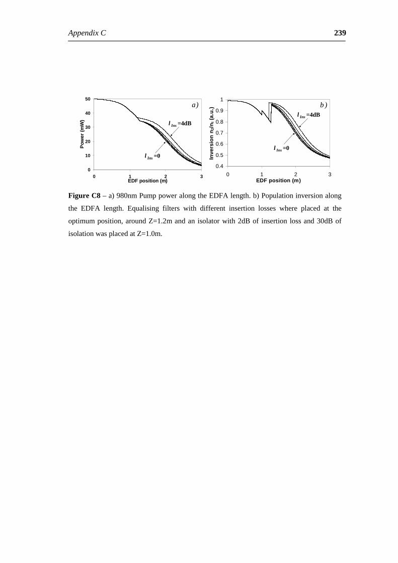
AppendixC 239
0
10
20
30
40
50
0 1 2 3EDFposition(m)
Pow
er(m
W)
a)
l Ins =4dB
l Ins =0
0.4
0.5
0.6
0.7
0.8
0.9
1
0 1 2 3EDFposition(m)
Inve
rsio
nn
2/n
t(a.
u.) b)
l Ins =4dB
l Ins =0
FigureC8–a)980nmPumppoweralongtheEDFAlength.b)Populationinversionalong
the EDFA length. Equalising filters with different insertion losses where placed at the
optimumposition,aroundZ=1.2mandan isolatorwith2dBof insertion lossand30dBof
isolationwasplacedatZ=1.0m.
AppendixD
Add-Dropsimulations
Thefiguresillustratedinthisappendixrefertochapter8.
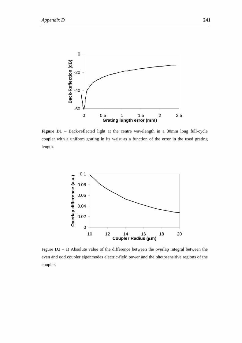
AppendixD 241
-60
-40
-20
0
0 0.5 1 1.5 2 2.5Gratinglengtherror(mm)
Bac
k-R
efle
ctio
n(d
B)
Figure D1 – Back-reflected light at the centre wavelength in a 30mm long full-cycle
coupler with a uniform grating in its waist as a function of the error in the used grating
length.
0
0.02
0.04
0.06
0.08
0.1
10 12 14 16 18 20CouplerRadius(µµµµm)
Ove
rlap
diff
eren
ce(a
.u.)
FigureD2–a)Absolutevalueofthedifferencebetween theoverlap integralbetween the
evenandoddcouplereigenmodeselectric-fieldpowerandthephotosensitiveregionsofthe
coupler.
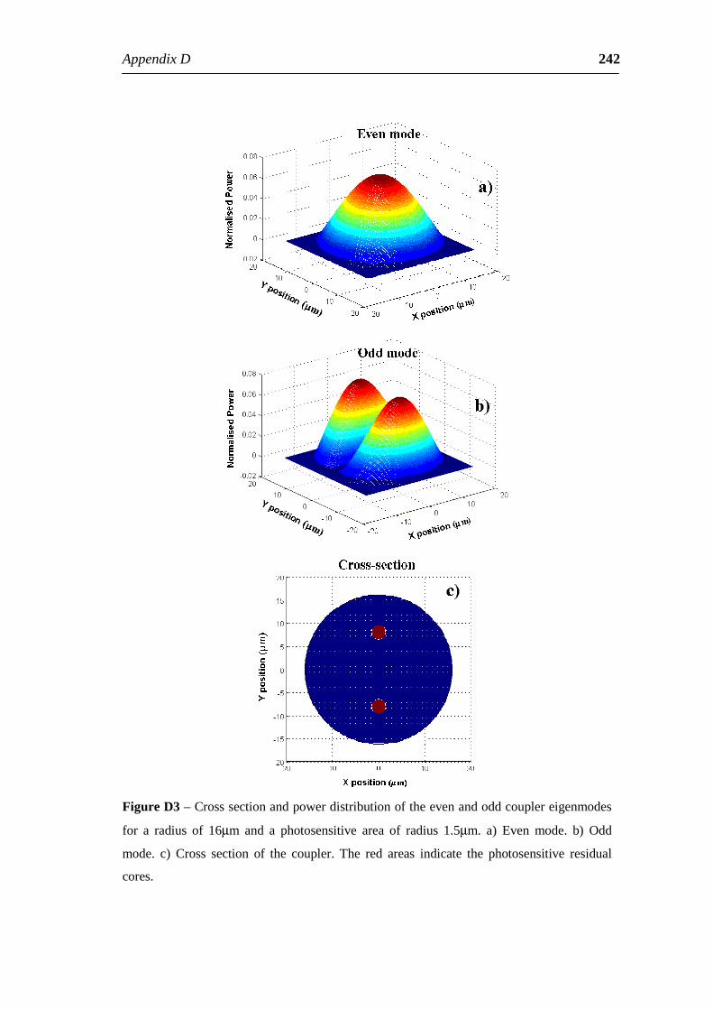
AppendixD 242
FigureD3–Crosssectionandpowerdistributionoftheevenandoddcouplereigenmodes
for a radius of 16µm and a photosensitive area of radius 1.5µm. a) Even mode. b) Odd
mode. c) Cross section of the coupler. The red areas indicate the photosensitive residual
cores.
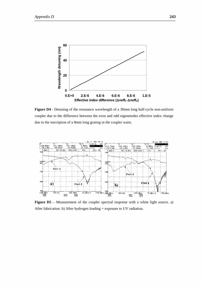
AppendixD 243
0
20
40
60
0.E+0 2.E-6 4.E-6 6.E-6 8.E-6 1.E-5Effectiveindexdifference(∆∆∆∆neffe-∆∆∆∆neffo)
Wav
elen
gth
detu
ning
(nm
)
FigureD4-Detuningoftheresonancewavelengthofa30mmlonghalf-cyclenon-uniform
couplerduetothedifferencebetweentheevenandoddeigenmodeseffectiveindexchange
duetotheinscriptionofa8mmlonggratinginthecouplerwaist.
Figure D5 – Measurement of the coupler spectral response with a white light source. a)
Afterfabrication.b)Afterhydrogenloading+exposuretoUVradiation.
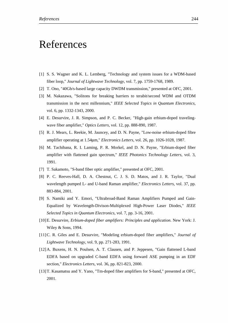
References 244
References
[1] S.S.Wagner andK.L.Lemberg, "Technologyand system issues foraWDM-based
fiberloop,"JournalofLightwaveTechnology,vol.7,pp.1759-1768,1989.
[2] T.Ono,"40Gb/s-basedlargecapacityDWDMtransmission,"presentedatOFC,2001.
[3] M. Nakazawa, "Solitons for breaking barriers to terabit/second WDM and OTDM
transmission in the next millennium," IEEE SelectedTopics in Quantum Electronics,
vol.6,pp.1332-1343,2000.
[4] E. Desurvire, J. R. Simpson, and P. C. Becker, "High-gain erbium-doped traveling-
wavefiberamplifier,"OpticsLetters,vol.12,pp.888-890,1987.
[5] R.J.Mears,L.Reekie,M.Jauncey,andD.N.Payne,"Low-noiseerbium-dopedfibre
amplifieroperatingat1.54µm,"ElectronicsLetters,vol.26,pp.1026-1028,1987.
[6] M. Tachibana, R. I. Laming, P. R. Morkel, and D. N. Payne, "Erbium-doped fiber
amplifier with flattened gain spectrum," IEEE Photonics Technology Letters, vol. 3,
1991.
[7] T.Sakamoto,"S-bandfiberopticamplifier,"presentedatOFC,2001.
[8] P. C. Reeves-Hall, D. A. Chestnut, C. J. S. D. Matos, and J. R. Taylor, "Dual
wavelengthpumpedL-andU-bandRamanamplifier,"ElectronicsLetters,vol.37,pp.
883-884,2001.
[9] S. Namiki and Y. Emori, "Ultrabroad-Band Raman Amplifiers Pumped and Gain-
Equalized by Wavelength-Divison-Multiplexed High-Power Laser Diodes," IEEE
SelectedTopicsinQuantumElectronics,vol.7,pp.3-16,2001.
[10]E.Desurvire,Erbium-dopedfiberamplifiers:Principlesandapplication.NewYork:J.
Wiley&Sons,1994.
[11]C. R. Giles and E. Desurvire, "Modeling erbium-doped fiber amplifiers," Journal of
LightwaveTechnology,vol.9,pp.271-283,1991.
[12]A. Buxens, H. N. Poulsen, A. T. Clausen, and P. Jeppesen, "Gain flattened L-band
EDFA based on upgraded C-band EDFA using forward ASE pumping in an EDF
section,"ElectronicsLetters,vol.36,pp.821-823,2000.
[13]T.KasamatsuandY.Yano,"Tm-dopedfiberamplifiersforS-band,"presentedatOFC,
2001.
References 245
[14]M. Yamada, T. Kanamori, Y. Terunuma, K. Oikawa, M. Shimizu, S. Sudo, and K.
Sagawa, "Fluoride-Based Erbium-Doped Fiber Amplifier with Inherently Flat Gain
Spectrum,"IEEEPhotonicsTechnologyLetters,vol.8,pp.882-884,1996.
[15]D.Bayart,B.Clesca,L.Hamon,andJ.L.Beylat,"Experimental Investigationof the
GainFlatnessCharacteristics for1.55mmErbium-DopedFluorideFiberAmplifiers,"
IEEEPhotonicsTechnologyLetters,vol.6,pp.613-615,1994.
[16]H.S.Kim,S.H.Yun,H.K.Kim,N.Park,andB.Y.Kim,"Dynamicgainequalization
oferbium-dopedfiberamplifierwithall-fiberacousto-optic tunablefilters,"presented
atOFCtechnicaldigest,1998.
[17]H. S. Kim, S. H. Yun, H. K. Park, and B. Y. Kim, "Actively gain-flattened erbium-
dopedfiberamplifierover35nmbyusingall-fiberacousto-optictunablefilters,"IEEE
PhotonicsTechnologyLetters,vol.10,pp.790-792,1998.
[18]R. Feced, C. Alegria, R. I. Laming, and M. N. Zervas, "Acoustooptic Attenuation
Filters Based on Tapered Optical Fibers," IEEE Selected Topics in Quantum
Electronics,vol.5,pp.1278-1288,1999.
[19]C.Alegria,R.Feced,M.N.Zervas,R. I.Laming,andS.G.Farwell,"Acousto-optic
filtersbasedonmulti-tapered fibre structures,"ElectronicsLetters,vol.35,pp.1006-
1007,1999.
[20]S.-K.LiawandY.-K.Chen,"PassiveGain-EqualisedWide-BandErbium-DopedFiber
AmplifierUsingSamarium-DopedFiber,"IEEEPhotonicsTechnologyLetters,vol.8,
pp.879-881,1996.
[21]P. D. Greene and H. N. Rourke, "Tailoring long period optical fibre gratings for
flatteningEDFAgainspectra,"ElectronicsLetters,vol.35,pp.1373-1374,1999.
[22]M.Rochette,M.Guy,S.Larochelle,J.Lauzon,andF.Trépanier,"Gainequalizationof
EDFA's with Bragg gratings," IEEE Photonics Technology Letters, vol. 11, pp. 536-
538,1999.
[23]P. F. Wysocki, J. B. Judkins, R. P. Espindola, M. Andrejco, and A. M. Vengsarkar,
"Broad-band erbium-doped fiber amplifier flattened beyond 40nm using long-period
gratingfilter,"IEEEPhotonicsTechnologyLetters,vol.9,pp.1343-1345,1997.
[24]J.E.FordandJ.A.Walker,"Dynamicspectralpowerequalizationusingmicro-opto-
mechanics,"IEEEPhotonicsTechnologyLetters,vol.10,pp.1440-1442,1998.
[25]P. M. Schiffer, C. R. Doerr, L. W. Stulz, M. A. Cappuzzo, E. J. Laskowski, A.
Paunescu,L.T.Gomez,andJ.V.Gates,"Smartdynamicwavelengthequalizerbased
References 246
onanintegratedplanaropticalcircuitforuseinthe1550-nmregion,"IEEEPhotonics
TechnologyLetters,vol.11,pp.1150-1152,1999.
[26]S. H. Yun, B. W. Lee, H. K. Kim, and B. Y. Kim, "Dynamic erbium-doped fiber
amplifierbasedonactivegainflatteningwithfiberacoustooptictunablefilters,"IEEE
PhotonicsTechnologyLetters,vol.11,pp.1229-1231,1999.
[27]S.K.Liaw,K.P.Ho,andS.Chi,"Dynamicpower-equalizedEDFAmodulebasedon
strain tunable fiberBragggratings," IEEEPhotonicsTechnologyLetters, vol. 11, pp.
797-799,1999.
[28]J.-M.Jouanno,D.Zauner,andM.Kristensen,"LowCrosstalkPlanarOpticalAdd-Drop
MultiplexerFabricatedwithUV-InducedBraggGratings,"ElectronicsLetters,vol.33,
pp.2120-2121,1997.
[29]J.Albert,F.Bilodeau,D.C.Johnson,K.O.Hill,K.Hattori,T.Kitagawa,Y.Hibino,
andM.Abe,"Low-LossPlanarLightwaveCircuitOADMwithHighIsolationandNo
Polarisation Dependence," IEEE Photonics Technology Letters, vol. 11, pp. 346-348,
1999.
[30]Y.Hibino,T.Kitagawa,K.O.Hill,F.Bilodeau,B.Malo,J.Albert,andD.C.Johnson,
"WavelengthDivisionMultiplexerwithPhotoinducedBraggGratingsFabricated in a
Planar-Lightwave-Circuit-Type Asymmetric Mach-Zehnder Interferometer on Si,"
IEEEPhotonicsTechnologyLetters,vol.8,pp.84-86,1996.
[31]T.Erdogan,T.A.Strasser,M.A.Milbrodt,E.J.Laskowski,C.H.Henry,andG.E.
Kohnke, "Integrated-opticalMach-Zehnderadd-drop filter fabricatedbya singleUV-
inducedgratingexposure,"AppliedOptics,vol.36,pp.7838-7845,1997.
[32]W.D.Zhong,S.Dods,J.P.R.Lacey,andR.S.Tucker,"Reconfigurablemultichannel
add-drop multiplexer with improved performance," Electronics Letters, vol. 32, pp.
1477-1478,1996.
[33]H. Takahashi, S. Susuki, K. Kato, and I. Nishi, "Arrayed-Waveguide Grating for
Wavelength Division Multi/Demultiplexer with Nanometre Resolution," Electronics
Letters,vol.26,pp.87-88,1990.
[34]K. Okamoto, M. Okuno, A. Himeno, and Y. Ohmori, "16-channel optical add/drop
multiplexer consisting of arrayed-waveguide gratings and double-gate switches,"
ElectronicsLetters,vol.32,pp.1471-1472,1996.
[35]C. R. Doerr, L. W. Stulz, J. Gates, M. Cappuzzo, E. Laskowski, L. Gomez, A.
Paunescu,A.White,andC.Narayanan,"ArrayedWaveguideLensWavelengthAdd-
DropinSilica,"IEEEPhotonicsTechnologyLetters,vol.11,pp.557-559,1999.
References 247
[36]C.R.Doerr,L.W.Stulz,M.Cappuzzo,E.Laskowski,A.Paunescu,L.Gomez,J.V.
Gates,S.Shunk,andA.E.White,"40-WavelengthAdd-DropFilter,"IEEEPhotonics
TechnologyLetters,vol.11,pp.1437-1439,1999.
[37]T. Mizuochi, T. Kitayama, K. Shimizu, and K. Ito, "Interferometric Crosstalk-Free
OpticalAdd/DropMultiplexerUsingMach-Zehnder-BasedFiberGratings,"Journalof
LightwaveTechnology,vol.16,pp.265-276,1998.
[38]L.Dong,P.Hua,T.A.Birks,L.Reekie,andP.S.J.Russell,"NovelAdd/DropFilters
for Wavelength-Division-Multiplexing Optical Fiber Systems Using a Bragg Grating
AssistedMismatchedCoupler,"IEEEPhotonicsTechnologyLetters,vol.8,pp.1656-
1658,1996.
[39]A.S.Kewitsch,G.A.Rakuljic,P.A.Willems,andA.Yariv,"All-fiberzero-insertion-
lossadd-dropfilterforwavelength-divisionmultiplexeing,"OpticsLetters,vol.23,pp.
106-108,1998.
[40]B.Ortega,L.Dong,andL.Reekie,"All-fiberopticaladd-dropmultiplexerbasedona
selectivefusedcouplerandasinglefiberBragggrating,"AppliedOptics,vol.37,pp.
7712-7717,1998.
[41]F. Bakhti, X. Daxhelet, P. Sansonetti, and S. Lacroix, "Influence of Bragg grating
locationinfused100%couplerforaddanddropmultiplexerrealization,"presentedat
OFC,1998.
[42]F.Bakhti,P.Sansonetti,C.Sinet,L.Gasca,L.Martineau,S.Lacroix,X.Daxhelet,and
F. Gonthier, "Optical add/drop multiplexer based on UV-written Bragg grating in a
fused100%coupler,"ElectronicsLetters,vol.33,pp.803-804,1997.
[43]S.Y.Kim,S.B.Lee,S.W.Kwon,S.S.Choi,andJ.Jeong,"Channel-switchingactive
add/dropmultiplexerwithtunablegratings,"ElectronicsLetters,vol.34,pp.104-105,
1998.
[44]J.T.Ahn,H.K.Lee,K.H.Kim,M.-Y.Jeon,D.S.Lim,andE.-H.Lee,"Astabilised
fibre-opticMach-Zehnder interferometer filterusingan independantstabilisation light
source,"OpticsCommunications,vol.157,pp.62-66,1998.
[45]S. Bethuys, L. Lablonde, L. Rivoallan, J. F. Bayon, L. Brilland, and E. Delavaque,
"Optical Add/Drop Multiplexer Based on UV-Written Bragg Gratings in Twincore
FibreMach-ZehnderInterferometer,"ElectronicsLetters,vol.34,pp.1250-1252,1998.
[46]S.Y.Kim,S.B.Lee,J.Chung,S.Y.Kim,I.J.Park,J.Jeong,andS.S.Choi,"Highly
Stable Optical Add/Drop Multiplexer Using Polarization Beam Splitters and Fiber
BraggGratings,"IEEEPhotonicsTechnologyLetters,vol.9,pp.1119-1121,1997.
References 248
[47]F.Bilodeau,D.C.Johnson,S.Thériault,B.Malo,J.Albert,andK.O.Hill,"AnAll-
Fiber Dense-Wavelength-Division Multiplexer/Demultiplexer Using Photoimprinted
BraggGratings,"IEEEPhotonicsTechnologyLetters,vol.7,pp.388-390,1995.
[48]R. Watanabe,K. Nosu, and Y. Fujii, "Optical Grating Multiplexer in the 1.1-1.5 µm
WavelengthRegion,"ElectronicsLetters,vol.16,pp.108-109,1980.
[49]J.SkaarandK.M.Risvik,"AGeneticAlgorithmfortheInverseProbleminSynthesis
ofFiberGratings,"JournalofLightwaveTechnology,vol.16,pp.1928-1932,1998.
[50]R.Feced,M.N.Zervas,andM.A.Muriel,"AnEfficientInverseScatteringAlgorithm
for the Design of Nonuniform Fiber Bragg Gratings," IEEE Journal of Quantum
Electronics,vol.35,pp.1105-1115,1999.
[51]T. Erdogan, "Optical add-drop multiplexer based on an asymmetric Bragg coupler,"
OpticsCommunications,vol.157,pp.249-264,1998.
[52]A. Iocco, H. G. Limberger, R. P. Salathé, L. A. Everall, K. E. Chisholm, J. A. R.
Williams,andI.Bennion,"BraggGratingFastTunableFilterforWavelengthDivision
Multiplexing,"JournalofLightwaveTechnology,vol.17,pp.1217-1221,1999.
[53]B.J.Eggleton,"RecentAdvancesofTunableFiberGratingTechnologies,"presentedat
BGPP,2001.
[54]C. R. Giles and M. Spector, "The Wavelength Add/Drop Multiplexer for Lightwave
Communication Networks," The Bell System Technical Journal, vol. January-March,
pp.207-229,1999.
[55]G. E. Keiser, "A Review of WDM technologies and applications," Optical Fiber
Technology,vol.5,pp.3-39,1999.
[56]D.Marcuse,Theoryofdielectricopticalwaveguides,2ndEditioned:AcademicPress,
1991.
[57]A.W.Snyder,"Polarisingbeamsplitterfromfused-tapercouplers,"ElectronicsLetters,
vol.21,pp.623-625,1985.
[58]A. Lord, I. J. Wilkinson, A. Ellis, D. Cleland, R. A. Garnham, and W. A. Stallard,
"Comparison of WDM coupler technologies for use in erbium-doped fibre amplifier
systems,"ElectronicsLetters,vol.26,pp.900-901,1990.
[59]S. G. Farwell, "Fused Tapered Fibre Optic Devices," in PhD Thesis, Universtity of
Southampton,1997.
[60]J. Bures, S. Lacroix, C. Veilleux, and J. Lapierre, "Some particular properties of
monomodefusedfibercouplers,"AppliedOptics,vol.23,pp.968-969,1984.
References 249
[61]T.E.Dimmick,G.Kakarantzas,T.A.Birks,andP.S.J.Russell,"Carbondioxidelaser
fabricationoffused-fibercouplersandtapers,"AppliedOptics,vol.38,pp.6845-6848,
1999.
[62]T. A. Birks, W. J. Wadsworth, and P. S. J. Russell, "Supercontinuum generation in
taperedfibers,"OpticsLetters,vol.25,pp.1415-1417,2000.
[63]J. D. Love, M. W. Henry, W. J. Stewart, R. J. Black, S. Lacroix, and F. Gonthier,
"Teperedsingle-modefibresanddevicesPart1:Adiabaticitycriteria,"IEEProceedings-
J,vol.138,pp.343-354,1991.
[64]T. A. Birks and Y. W. Li, "The Shape of Fiber Tapers," Journal of Lightwave
Technology,vol.10,pp.432-438,1992.
[65]W. K. Burns, M. Abebe, and C. A. Villarruel, "Parabolic model for shape of fiber
taper,"AppliedOptics,vol.24,pp.2753-2755,1985.
[66]R.P.Kenny,T.A.Birks,andK.P.Oakley,"ControlofOpticalFibreTaperShape,"
ElectronicsLetters,vol.27,pp.1654-1655,1991.
[67]S. Lacroix, F. Gonthier, and J. Bures, "Modeling of symmstric 2 x 2 fused-fiber
couplers,"AppliedOptics,vol.33,pp.8361-8369,1994.
[68]J. Bures, S. Lacroix, and J. Lapierre, "Analyse d'un coupleur bidirectionnel à fibres
optiquesmonomodesfusionnées,"AppliedOptics,vol.22,pp.1918-1922,1983.
[69]F. P. Payne, C. D. Hussey, and M. S. Yataki, "Modelling Fused Single-Mode-Fibre
Couplers,"ElectronicsLetters,vol.21,pp.461-462,1985.
[70]A.W.SnyderandX.-H.Zheng,"Opticalfibersofarbitrarycrosssections,"Journalof
theOpticalSocietyofAmericaA,vol.3,pp.600-609,1986.
[71]A. W. Snyder and X.-H. Zheng, "Fused Couplers of Arbitrary Cross-Section,"
ElectronicsLetters,vol.21,pp.1079-1080,1985.
[72]F. Gonthier, S. Lacroix, and J. Bures, "Numerical Calculations of Modes of Optical
Waveguides with Two-Dimensional Refractive Index Profiles by a Field Correction
Method,"OpticalandQuantumElectronics,vol.26,pp.S135-S149,1994.
[73]C.-C. Su, "A Surface Integral Equations Method Homogeneous Optical Fibers and
CoupledImageLinesofArbitraryCrossSections,"IEEETransactionsonMicrowave
TheoryanTechniques,vol.MTT-33,pp.1114-1119,1985.
[74]T.-L. Wu and H.-C. Chang, "Rigorous Analysis of Form Birefringence of Weakly
FusedFiber-OpticCouplers,"JournalofLightwaveTechnology,vol.13,pp.687-691,
1995.
References 250
[75]S.-W. Yang and H.-C. Chang, "Numerical Modeling of Weakly Fused Fiber-Optic
Polarization Beamsplitters-Part I: Accurate Calculation of Coupling Coefficients and
FormBirefringence,"JournalofLightwaveTechnology,vol.16,pp.685-690,1998.
[76]T.Erdogan,"Cladding-moderesonancesinshort-andlong-periodfibergratingfilters,"
JournaloftheOpticalSocietyofAmericaA,vol.14,pp.1760-1773,1997.
[77]C.R.Giles,"LightwaveApplicationsofFiberBraggGratings,"JournalofLightwave
Technology,vol.15,pp.1391-1404,1997.
[78]T. Erdogan, "Fiber Grating Spectra," Journal of Lightwave Technology, vol. 15, pp.
1277-1294,1997.
[79]H. Kogelnik, "Filter Response of Nonuniform Almost-Periodic Structures," The Bell
SystemTechnicalJournal,vol.55,pp.109-126,1976.
[80]A.YarivandP.Yeh,Opticalwavesincrystals:JohnWiley&SonsInc,1984.
[81]A.Yariv,"Coupled-ModeTheoryforGuided-WaveOptics,"IEEEJournalofQuantum
Electronics,vol.QE-9,pp.919-933,1973.
[82]M.Ibsen,R.Feced,P.Petropoulos,andM.N.Zervas,"99.9%Reflectivitydispersion-
lesssquare-filter fibreBragggratings forhighspeedDWDMnetworks,"presentedat
OFC,Baltimore,2000.
[83]J.Skaar,"SynthesisandCharacterizationofFibreBraggGratings,"PhDThesis,2000.
[84]P.J.Lemaire,R.M.Atkins,V.Mizrahi,andW.A.Reed,"HighPressureH2Loadingas
aTechnique forAchievingUltrahighUVPhotosensitivity andThermalSensitivity in
GeO2DopedOpticalFibres,"ElectronicsLetters,vol.29,pp.1191-1193,1993.
[85]F.Bilodeau,B.Malo,J.Albert,D.C.Johnson,K.O.Hill,Y.Hibino,M.Abe,andM.
Kawachi, "Photosensitization of Optical Fiber and Silica-on-Silicon/Silica
Waveguides,"OpticsLetters,vol.18,pp.953-955,1993.
[86]J. Stone, "Interactions of Hydrogen and Deuterium with Silica Optical Fibers: A
Review,"JournalofLightwaveTechnology,vol.LT-5,pp.712-733,1987.
[87]A. Iino,M.Kuwabara,andK.Kokura,"MechanismsofHydrogen-InducedLosses in
Silica-BasedOpticalFibers,"JournalofLightwaveTechnology,vol.8,pp.1675-1679,
1990.
[88]J.Canning,"PhotosensitizationandPhotostabilizationofLaser-InducedIndexChanges
inOpticalFibres,"OpticalFiberTechnology,vol.6,pp.275-289,2000.
[89]M. Berwick, C. N. Pannel, P. S. J. Russell, and D. A. Jackson, "Demonstration of
birefringent optical fibre frequency shifter employing torsional acoustic waves,"
ElectronicsLetters,vol.27,pp.713-715,1991.
References 251
[90]H. Sabert, L. Dong, and P. S. J. Russell, "Versatile acousto-optic flexural wave
modulator, filter and frequency shifter in dual-core fiber," International Journal of
Optoelectronics,vol.7,pp.189-194,1992.
[91]T.A.Birks,D.O.Culverhouse,S.G.Farwell,andP.S.J.Russell,"2X2Single-mode
fiberroutingswitch,"OpticsLetters,vol.21,pp.722-724,1996.
[92]T. A. Birks, S. G. Farwell, P. S. J. Russell, and C. N. Pannell, "Four-port fiber
frequency shifter with a null taper coupler," Optics Letters, vol. 19, pp. 1964-1966,
1994.
[93]T.A.Birks,P.S.J.Russell,andC.N.Pannell,"Lowpoweracousto-opticdevicebased
ona taperedsingle-modefiber,"IEEEPhotonicsTechnologyLetters,vol.6,pp.725-
727,1994.
[94]W.P.Risk,G.S.Kino,andH.J.Shaw,"Fiber-opticfrequencyshifterusingasurface
acousticwaveincidentatanobliqueangle,"OpticsLetters,vol.11,pp.115-117,1986.
[95]D.O.Culverhouse,S.G.Farwell,T.A.Birks,andP.S. J.Russell,"Four-port fused
taper acousto-optic devices using standard singlemode Telecomunications fibre,"
ElectronicsLetters,vol.31,pp.1279-1280,1995.
[96]S.G.Farwell,D.O.Culverhouse,T.A.Birks,andP.S.J.Russell,"Low-lossall-fibre
amplitudemodulatorat1.55mm,"ElectronicsLetters,vol.32,pp.577-578,1996.
[97]A.M.Vengsarkar,J.R.Pedrazzani,J.B.Judkins,P.J.Lemaire,N.S.Bergano,andC.
R.Davidson,"Long-periodfiber-grating-basedgainequalisers,"OpticsLetters,vol.21,
pp.336-338,1996.
[98]H.S.Kim,S.H.Yun, I.K.Kwang,andB.Y.Kim,"All-fiberacousto-optic tunable
notchfilterwithelectronicallycontrollablespectralprofile,"OpticsLetters,vol.22,pp.
1476-1478,1997.
[99]H. E. Engan, B. Y. Kim, J. N. Blake, and H. J. Shaw, "Propagation and optical
interactionofguidedacousticwavesintwo-modeopticalfibres,"JournalofLightwave
Technology,vol.6,pp.428-436,1988.
[100] T.A.Birks,P.S.J.Russell,andD.O.Culverhouse,"Theacousto-opticeffectin
single-modefibertapersandcouplers,"JournalofLightwaveTechnology,vol.14,pp.
2519-2529,1996.
[101] R.N.Thurston, "Elasticwaves in rodsandclad rods,"Journalof theAcoustical
SocietyofAmerica,vol.64,pp.1-37,1978.
References 252
[102] J. N. Blake, B. Y. Kim, H. E. Engan, and H. J. Shaw, "Analysis of intermodal
coupling in a two-mode fibre with periodic microbends," Optics Letters, vol. 12, pp.
281-283,1987.
[103] H. F. Taylor, "Bending Effects in Optical Fibers," Journal of Lightwave
Technology,vol.LT-2,pp.617-628,1984.
[104] H. Zech, "Theoretical investigation of the gain profile of erbium-doped fiber
amplifiers,"OpticalFiberTechnology,vol.1,pp.327-330,1995.
[105] H.Zech,"MeasurementTechniquefortheQuotientofCrossSectionsσe(λs)/σa(λs)
of Erbium-Doped Fibers," IEEE Photonics Technology Letters, vol. 7, pp. 986-988,
1995.
[106] W. L. Barnes, R. I. Laming, E. J. Tarbox, and P. R. Morkel, "Absorption and
Emission Cross Section of Er3+ Doped Silica Fibers," IEEE Journal of Quantum
Electronics,vol.27,pp.1004-1010,1991.
[107] R. E. Tench and M. Shimizu, "Fluorescence-Based Measurement of g*(l) for
Erbium-DopedFluorideFiberAmplifiers,"JournalofLightwaveTechnology,vol.15,
pp.1559-1564,1997.
[108] M. N. Zervas, R. I. Laming, and D. N. Payne, "Efficient Erbium-doped fiber
amplifiers incorporating an optical isolator," IEEE Journal of Quantum Electronics,
vol.11,pp.472-480,1995.
[109] J.H.Povlsen,A.Bjarklev,O.Lumholt,H.Vendeltorp-Pommer,K.Rottwitt,and
T.Rasmussen,"OptimizinggainandnoiseperformanceofEDFA'swithinsertionofa
filteroranisolator,"SPIEFiberLaserSourcesandAmplifiersIII,vol.1581,pp.107-
113,1991.
[110] C. Riziotis and M. N. Zervas, "Design Considerations in Optical Add/Drop
Multiplexers Based on Grating-Assited Null Couplers," Journal of Lightwave
Technology,vol.19,pp.92-104,2001.
[111] I.Baumann,J.Seifert,W.Nowak,andM.Sauer,"CompactAll-FiberAdd-Drop-
MultiplexerUsingFiberBraggGratings,"IEEEPhotonicsTechnologyLetters,vol.8,
pp.1331-1333,1996.
[112] C. Riziotis, P. G. R. Smith, and M. N. Zervas, "Performance characteristics of
interferrometric Bragg grating based OADMs in WDM transmission systems,"
presentedatBGPP,Stresa,Italy,2001.
[113] L.MartineauandS.Lacroix,"FabricationofHighlyGe-dopedFibreCouplersby
Fusing-TaperingTechnique,"ElectronicsLetters,vol.33,pp.798-800,1997.
References 253
[114] E.Marin,R.Ghosh,J.-P.Meunier,X.Daxhelet,andS.Lacroix,"BraggGratings
in 2 x 2 Symmetric Fused Fiber Couplers: Influence of the Tilt on the Wavelength
Response,"IEEEPhotonicsTechnologyLetters,vol.11,pp.1434-1436,1999.
[115] R.J.Orazi,S.D.Russell,T.T.Vu,andP.K.L.Yu,"UVfinetuningofnarrow
channel fused fibre wavelength division multiplexing couplers," Electronics Letters,
vol.33,pp.154-155,1997.
[116] S. J. Ashby, R. B. Charters, J. D. Love, F. Ladouceur, and M. C. Elias, "Large
wavelength shifts in UV-exposed 3dB and WDM fused taper fibre couplers,"
ElectronicsLetters,vol.33,pp.1696-1697,1997.
[117] H.Gnewuch,J.E.Roman,M.Hempstead,J.S.Wilkinson,andR.Ulrich,"Beat-
length measurement in directional couplers by thermo-optic modulation," Optics
Letters,vol.21,pp.1189-1191,1996.
[118] Y. Bourbin, A. Enard, M. Papuchon, and K. Thyagarajan, "The local absorption
thechnique: A straightforward characterisation method for many optical devices,"
JournalofLightwaveTechnology,vol.LT-5,pp.684-687,1987.
[119] N. Sahba and T. J. Rocket, "Infrared absorption coefficients of silica glasses,"
JournalAmericanCeramicSociety,vol.75,pp.209-212,1992.
[120] R.FecedandM.N.Zervas,"Efficientinversescatteringalgorithmforthedesignof
grating-assisted codirectional mode couplers," Journal of the Optical Society of
AmericaA,vol.17,pp.1573-1581,2000.
[121] A.SnyderandJ.D.Love,OpticalWaveguideTheory:ChapmanandHall,1983.
ListofPublications
ConferencePublications:
C Alegria, R Feced, M N Zervas and R I Laming, “ Acousto-optic effect in optical fibre
taperedstructuresforthedesignoffilters” ,IEEColloquium:Newdevelopmentsinoptical
amplifiers,London,November2nd1998.
C.Alegria,R.Feced,M.N.Zervas,R.I.Laming,“ Dynamicacousto-opticfiltersforgain
flattening of optical amplifiers” , Proc. II conferência de telecomunicações, Sesimbra-
Portugal,15-16April1999.
F.Ghiringhelli,C.Alegria,M.N.Zervas,“ Effectofphaseshiftperturbationsandcomplex
localtimedelayinfiberBragggratings” ,Proc.BGPP2001,StresaCongressCenter,Stresa-
Italy,4-6July2001.
C. Alegria, F. Ghiringhelli, M. N. Zervas, “ Non-Destructive Characterisation of Fibre
Couplers” , ECOC 2001, Rai Congress Center, Amsterdam-Holand, 30 September to 4
October2001.–Invitedpaper
C.Alegria,M.N.Zervas,R.Feced “ GratingAdd-DropMultiplexerbasedonaCompact
Non-UniformFusedFiberCoupler” ,acceptedtoOFC2002,Anaheim,USA.
JournalPublications:
R.Feced,C.Alegria,M.N.Zervas,R. I.Laming,"Acoustoopticattenuationfiltersbased
ontaperedopticalfibres",IEEEJournalofSelectedTopicsinQuantumElectronics,Vol.5,
No.5,pp.(1999).
C. Alegria, R. Feced, M. N. Zervas, R. I. Laming, S. G. Farwell, "Acousto-optic filters
basedonmulti-taperedfibrestructures",ElectronicsLetters,Vol.35,No.12,pp.(1999).
C. Alegria, M. N. Zervas, “ Non-destructive Coupler Characterisation Technique” ,
submittedtoJournalofLightwaveTechnology.
Patentapplications:
C. Alegria, M. N. Zervas, University of Southampton, “ Methods and apparatus for
analysingwaveguidecouplers” ,Filed14thSeptember2001.EuropeanPatentapplicationNo.
01306893.7-1236.