university of tartu - tuit.ut.ee angular velocity spin up to 360 deg/s.. . . . . . . . . . . . . . ....
TRANSCRIPT

University of Tartu
Faculty of Science and Technology
Institute of Technology
Ikechukwu Ofodile
Design and Comparison of Attitude Control
Modes for ESTCube-2
Master’s Thesis (30 ECTS)
(Robotics and Computer Engineering)
Supervisors:
Dr. Andris Slavinskis
Assoc. Prof. Gholamreza Anbarjafari
Tartu 2017

Contents
Contents i
List of Figures iv
List of Tables vi
Abbreviations vii
Symbols viii
1 Introduction 3
1.1 Motivation . . . . . . . . . . . . . . . . . . . . . . . . . . . . . . . . 3
1.2 Background and Literature Survey . . . . . . . . . . . . . . . . . . 4
1.3 Aim and Objectives . . . . . . . . . . . . . . . . . . . . . . . . . . . 6
1.4 Thesis Outline . . . . . . . . . . . . . . . . . . . . . . . . . . . . . . 6
2 Background to SpacecraftAttitude Control 8
2.1 Introduction . . . . . . . . . . . . . . . . . . . . . . . . . . . . . . . 8
2.2 Reference Frame . . . . . . . . . . . . . . . . . . . . . . . . . . . . 8
2.2.1 Earth-Centered Inertial Reference Frame (ECIF) . . . . . . 9
2.2.2 Earth-Centered Earth Fixed Reference frame (ECEF) . . . . 9
2.2.3 Local-Vertical Local-Horizontal Reference frame (LVLH) . . 9
2.2.4 Spacecraft Body Reference frame (SBRF) . . . . . . . . . . 9
2.3 Attitude Parameterization . . . . . . . . . . . . . . . . . . . . . . . 10
2.3.1 Direction Cosine Matrix (DCM) . . . . . . . . . . . . . . . . 10
2.3.2 Euler Angles . . . . . . . . . . . . . . . . . . . . . . . . . . . 10
2.3.3 Unit Quaternions . . . . . . . . . . . . . . . . . . . . . . . . 12
2.3.4 Quaternion Rotation . . . . . . . . . . . . . . . . . . . . . . 13
2.3.5 Error Quaternion . . . . . . . . . . . . . . . . . . . . . . . . 14
2.4 Sensors . . . . . . . . . . . . . . . . . . . . . . . . . . . . . . . . . . 15
2.4.1 Gyroscopes . . . . . . . . . . . . . . . . . . . . . . . . . . . 15
2.4.2 Accelerometers . . . . . . . . . . . . . . . . . . . . . . . . . 15
i

ii
2.4.3 Magnetometers . . . . . . . . . . . . . . . . . . . . . . . . . 16
2.4.4 Sun sensor . . . . . . . . . . . . . . . . . . . . . . . . . . . . 16
2.4.5 Star tracker . . . . . . . . . . . . . . . . . . . . . . . . . . . 16
2.5 Actuators . . . . . . . . . . . . . . . . . . . . . . . . . . . . . . . . 16
2.5.1 Reaction Wheels . . . . . . . . . . . . . . . . . . . . . . . . 16
2.5.2 Magnetic Coils . . . . . . . . . . . . . . . . . . . . . . . . . 17
2.5.3 Cold Gas Thruster . . . . . . . . . . . . . . . . . . . . . . . 18
3 Spacecraft Modeling 19
3.1 Kepler And Newton’s Laws . . . . . . . . . . . . . . . . . . . . . . 19
3.2 Inertia Matrix . . . . . . . . . . . . . . . . . . . . . . . . . . . . . . 20
3.3 Environmental Models . . . . . . . . . . . . . . . . . . . . . . . . . 21
3.3.1 Earth’s Geomagnetic Field . . . . . . . . . . . . . . . . . . . 21
3.3.2 Gravity-Gradient Torque . . . . . . . . . . . . . . . . . . . . 23
3.3.3 Aerodynamic Torque . . . . . . . . . . . . . . . . . . . . . . 24
3.3.4 Solar Radiation Torque . . . . . . . . . . . . . . . . . . . . . 25
3.3.5 Residual Magnetic Torque . . . . . . . . . . . . . . . . . . . 25
3.4 Dynamics . . . . . . . . . . . . . . . . . . . . . . . . . . . . . . . . 26
3.5 Kinematics . . . . . . . . . . . . . . . . . . . . . . . . . . . . . . . 27
3.6 Linearization . . . . . . . . . . . . . . . . . . . . . . . . . . . . . . 28
4 Attitude Control forESTCube-2 31
4.1 Description and Control Specifications for ESTCube-2 . . . . . . . . 31
4.2 Detumbling Controller Designs . . . . . . . . . . . . . . . . . . . . . 31
4.2.1 B-dot Controller Design . . . . . . . . . . . . . . . . . . . . 32
4.2.2 P Controller Designs . . . . . . . . . . . . . . . . . . . . . . 33
4.2.3 PD Controller Designs . . . . . . . . . . . . . . . . . . . . . 34
4.3 Pointing Controller Designs . . . . . . . . . . . . . . . . . . . . . . 34
4.3.1 PD Controller . . . . . . . . . . . . . . . . . . . . . . . . . . 35
4.3.2 Linear Quadratic Regulator Design . . . . . . . . . . . . . . 35
4.4 Cross Product Control Law . . . . . . . . . . . . . . . . . . . . . . 39
4.5 Spin-up Controller Designs . . . . . . . . . . . . . . . . . . . . . . . 39
5 Simulation Results and Controller Comparison 43
5.1 B-dot Controller Analysis . . . . . . . . . . . . . . . . . . . . . . . 43
5.2 PD Controller Analysis . . . . . . . . . . . . . . . . . . . . . . . . . 43
5.2.1 PD performance with Magnetorquers . . . . . . . . . . . . . 44
5.2.2 PD performance with saturated Reaction Wheels . . . . . . 48
5.2.3 PD performance with unsaturated wheels . . . . . . . . . . . 51
5.3 Cross Product Control Analysis . . . . . . . . . . . . . . . . . . . . 54
5.4 LQR Analysis . . . . . . . . . . . . . . . . . . . . . . . . . . . . . . 57
5.5 Spin-up Controller Analysis . . . . . . . . . . . . . . . . . . . . . . 62
6 Conclusion & Future Work 65

iii
6.1 Conclusion . . . . . . . . . . . . . . . . . . . . . . . . . . . . . . . . 65
6.2 Future Work . . . . . . . . . . . . . . . . . . . . . . . . . . . . . . . 66
A Controllability Analysis 71
B Linear Programming Code. 72
C Nadir Pointing Satellite Model With Reaction Wheels 75
C.1 Model with Reaction Wheels . . . . . . . . . . . . . . . . . . . . . . 75
C.2 Model with Magnetorquers . . . . . . . . . . . . . . . . . . . . . . . 76
D Abstracts Accepted for Oral Presentations 78
D.1 Abstract for 68th International Astronautical Congress 2017 - TetherDeployment Using High Spin Rate Control For Interplanetary Nanosatel-lite Missions . . . . . . . . . . . . . . . . . . . . . . . . . . . . . . . 78
D.2 Abstract for 6th iCubeSat Workshop 2017 - ESTCube-2 Nanosatel-lite Attitude Control for Interplanetary Missions . . . . . . . . . . . 79

List of Figures
1.1 ESTCube-2 exploded view [1]. . . . . . . . . . . . . . . . . . . . . . 5
3.1 Earth’s Magnetic Dipole [2]. . . . . . . . . . . . . . . . . . . . . . . 22
4.1 Attitude Control block diagram with feedback. . . . . . . . . . . . . 35
4.2 LQR design from linearization. . . . . . . . . . . . . . . . . . . . . 37
4.3 LQR controller on nonlinear spacecraft model. . . . . . . . . . . . . 37
4.4 LQR controller design algorithm. . . . . . . . . . . . . . . . . . . . 38
5.1 Detumbling of Satellite with Bdot Control . . . . . . . . . . . . . . 44
5.2 Quaternion Attitude during detumbling phase. . . . . . . . . . . . . 44
5.3 Magnetorquer Torque response during detumbling phase. . . . . . . 45
5.4 PD controller Angular velocity for Detumbling/Pointing with Mag-netorquer. . . . . . . . . . . . . . . . . . . . . . . . . . . . . . . . . 46
5.5 PD controller Quaternion Attitude for Detumbling/Pointing withMagnetorquer . . . . . . . . . . . . . . . . . . . . . . . . . . . . . . 46
5.6 Magnetorquer Torque response. . . . . . . . . . . . . . . . . . . . . 47
5.7 PD controller Angular velocity for Detumbling/Pointing with reac-tion wheels saturated . . . . . . . . . . . . . . . . . . . . . . . . . . 48
5.8 PD controller Quaternion Attitude for Detumbling/Pointing withreaction wheels saturated . . . . . . . . . . . . . . . . . . . . . . . . 49
5.9 Angular momentum showing reaction wheels saturated . . . . . . . 49
5.10 Reation Wheel saturated torque response . . . . . . . . . . . . . . . 50
5.11 PD controller Angular velocity for Detumbling/Pointing with reac-tion wheels . . . . . . . . . . . . . . . . . . . . . . . . . . . . . . . 51
5.12 PD controller Quaternion Attitude for Detumbling/Pointing withreaction wheels . . . . . . . . . . . . . . . . . . . . . . . . . . . . . 52
5.13 Angular momentum showing reaction wheels . . . . . . . . . . . . . 52
5.14 Reation Wheel torque response . . . . . . . . . . . . . . . . . . . . 53
5.15 Angular velocity response while unloading Reaction Wheels withmagnetorquers . . . . . . . . . . . . . . . . . . . . . . . . . . . . . . 54
5.16 Quaternion Attitude during Reaction Wheel unloading with Mag-netorquers . . . . . . . . . . . . . . . . . . . . . . . . . . . . . . . . 55
iv

List of Figures v
5.17 Reaction Wheels angular momentum saturated and unloading withmagnetorquers . . . . . . . . . . . . . . . . . . . . . . . . . . . . . . 55
5.18 Reaction Wheel torque response during unloading . . . . . . . . . . 56
5.19 Magnetorquer torque response with Reaction Wheel unloading . . . 56
5.20 Quaternion Step response (weighting matrices Q = diag[1,1,1,1,1,1], R = diag[1, 1, 1]) . . . . . . . . . . . . . . . . . . . . . . . . . . 58
5.21 Angular Velocity Step response (weighting matrices Q = diag[1,1,1,1,1,1], R = diag[1, 1, 1] ). . . . . . . . . . . . . . . . . . . . . . . . . . 58
5.22 Angular Velocity LQR controller performance with noise. . . . . . . 59
5.23 Quaternion Attitude LQR controller response with noise. . . . . . . 59
5.24 Angular Velocity LQR controller performance. . . . . . . . . . . . . 60
5.25 Angular Velocity LQR controller performance with Magnetorquers. 60
5.26 Quaternion Attitude LQR controller response with Magnetorquers. 61
5.27 Magnetorquer Torque response with LQR. . . . . . . . . . . . . . . 61
5.28 Angular Velocity Spin up to 110 deg/s. . . . . . . . . . . . . . . . . 63
5.29 Angular Velocity Spin up to 180 deg/s. . . . . . . . . . . . . . . . . 63
5.30 Angular Velocity Spin up to 360 deg/s. . . . . . . . . . . . . . . . . 64

List of Tables
5.1 PD Performance Overview. . . . . . . . . . . . . . . . . . . . . . . . 45
5.2 Satellite Parameters to obtain LQR controller gain. . . . . . . . . . 57
5.3 Spin rate simulation result. . . . . . . . . . . . . . . . . . . . . . . . 62
6.1 Overview of Designed Controllers. . . . . . . . . . . . . . . . . . . . 65
vi

Abbreviations
ADCS Attitude Determination and Control System
ACS Attitude Control System
COM Communication
EPS Electrical Power System
ECIF Earth Centered Inertial Reference Frame
LVLH Local Vertical Local Horizontal
SBRF Spacecraft Body Reference Frame
LEO Low Earth Orbit
GEO Geosynchronous Earth Orbit
MT Magnetorquer
RW Reaction Wheel
PID Proportional Integral Derivative
LQR Linear Quadratic Regulator
vii
Symbols
e axis directional unit vector
Ω() skew-symmetric cross-product matrix
a distance m
b Earth’s Magnetic Field vector T
µf Earth’s magnetic field’s dipole strength Wb ·m
h Angular momentum N ·m · s
he Angular momentum error N ·m · s
J Moment of Inertia matrix kg ·m2
m Magnetorquer dipole vector A ·m2
T Orbital period s
ωi Inertial Angular velocity rads−1
ωo Orbital Angular velocity rads−1
Tc Control Torque N ·m
Td Disturbance Torque N ·m
cp Centre of Pressure
cg Centre of Mass
viii

UNIVERSITY OF TARTU
Abstract
Faculty of Science and Technology
Institute of Technology
Master of Science
Design and Comparison of Attitude Control Modes for ESTCube-2
by Ikechukwu Ofodile
This thesis presents the attitude control problem of ESTCube-2. ESTCube-2 is a
3U CubeSat with a size of 10 x 10 x 30 cm and a weight of about 4 kg. It is the
second satellite to be developed by the ESTCube Team and will be equipped with
the E-Sail payload for the plasma break experiment, Earth observation camera, a
high speed communication system, and a cold gas propulsion module. The satellite
will make use of 3 electromagnetic coils, 3 reaction wheels and the cold gas thruster
as actuators.
The primary purpose of this work was to develop and compare control laws to fulfill
the attitude control requirements of the ESTCube-2 mission. To achieve this, the
spacecraft dynamics and environmental models are derived and analyzed. PD like
controllers and LQR optimal controls are designed to fulfill the pointing require-
ments of the satellite in addition to the B-dot detumbling control law. Angular
rate control law to spin up the satellite for tether deployment is also derived and
presented. Simulations of the different controllers shows the performance with dis-
turbances also added to the system. Finally recommendations and optimal control
situations are presented based on the results.
Keywords: CubeSat, ESTCube-2, Attitude Control, High spin rate, LQR.
CERCS: P170, T125, T320

Abstract 2
Abstract
ESTCube-2 asendi kontrolli reziimide disain ja vordlus
See too esitab ESTCube-2 asendi kontrolli probleemi. ESTCube-2 on 3U Cube-
Sat, mille suurus on 10x10x10 cm ning selle kaaluks on 4 kg. See on teine satelliit
valmistatud ESTCube meeskonna poolt ning selle pardal on erinevad kasulikud
lastid: plasma pidur, kaks maavaatluskaamerat, kommunikatsioonisusteem suurte-
mateks andmevahetuskiirusteks ning kulma gaasi toukur. Satelliit kasutab asendi
kontrollimiseks kolme elektromagnetmahist, kolme reaktsiooniratast ning kulma
gaasi toukurit.
Too peamine eesmark oli arendada ning vorrelda erinevaid asendi kontrolli algo-
ritme, mis taidaksid ESTCube-2 missiooni nouded. Selle saavutamiseks tuletati
ning analuusiti sateliidi dunaamika ning keskkonna mudeleid. B-dot poorlemise
vahendamiseks ning suunamise kontrolleriteks arendati PD-regulaatoril ning LQ-
regulaatoril pohinevaid kontrollereid. Tuletati ning esitati poorlemiskiiruse kon-
trollimise seadused, et satelliiti poorlema panna. Viidi labi simulatsioonid, mil-
lele on lisatud erinevad haired, iseloomustavad susteemi toimimist. Lopetuseks
antakse toos soovitused ning optimaalsed kontrolli olukorrad, mis pohinevad eel-
nevatel tulemustel
Keywords: CubeSat, ESTCube-2, Attitude Control, High spin rate, LQR.
CERCS: P170, T125, T320
1 Introduction
1.1 Motivation
Since it’s inception in 2008, the ESTCube project is a student project which is now
aimed at getting students involved in understanding the concepts of space tech-
nology and it emerging technologies with scientific and engineering impacts. The
ESTCube-1 student satellite project was launched on the 7 May 2013, and involved
students from the University of Tartu, Estonian Aviation Academy, Tallinn Uni-
versity of Technology and Estoninan University of Life Sciences as well as instruc-
tors and experts from different countries [3]. The main mission of the ESTCube-1
satellite was to test the Electric Solar wind sail (E-sail) developed by Pekka Jan-
hunen [4]. Students had the opportunity to write their Bachelors’ and Masters’
Thesis on various parts and subsystems of the satellite including the ADCS, EPS,
COM etc. As a student of the Robotics and Computer Engineering Master’s Pro-
gram of the University of Tartu, this thesis will show forth the knowledge I have
gained by participating in the ESTCube-2 project relating to spacecraft dynamics
and implementation using quaternions as well as controllers to be used on the
satellite for attitude control.
3

Chapter 1: Introduction 4
1.2 Background and Literature Survey
The increased research interests and innovations in space technology and explo-
ration, has driven a increase in development of nanosatellites (mass of 1-10kg) and
microsatellites. These satellites are mostly deployed in Low Earth Orbit (LEO) for
various mission objectives such as weather forcasting, telecommunications, earth
observation, environmental and scientific research purposes. The development of
CubeSat class of nanosatellites, began in 1999 in California [5]. A great success was
achieved in a collaborative effort between California Polytechnic State University
and Stanford university to develop an efficient and inexpensive satellite. CubeSats
have now recently being used as a great opportunity for researchers and universi-
ties to advance on the wide range of experimental and research opportunities in
space technology.
Satellites deployed for various missions have to be equipped with a reliable Atti-
tude Control System (ACS) to meet the requirements of the mission. Hence the
ADCS is regarded as an important subsystem of satellites. It is often expressed as
visual perspective or feeling of the satellites in space. The ACS performs several
operational modes and must maintain the attitude control even in the presence of
disturbance torques on the satellite.
Several works and university thesis reports have aimed to address varying attitude
determination and control design objectives and problems. While earlier works
are based on euler angle model, recent designs have discussed the design with
quaternion models [6–11]. Quaternion applications have been widely used in field
of computer science in areas of robotics, computer vision, motion planning, swarm
robotics. The use of quaternions in spacecraft model has significant advantage
over the Euler angle representation. The quaternion attitude representation, does
not depend on rotation sequence as in the case of Euler angle representation, and
does not have a singular point for any attitude. This advantages will be described
in this thesis work.
The application of Lyapunov based functions to design varying control laws have
Chapter 1: Introduction 5
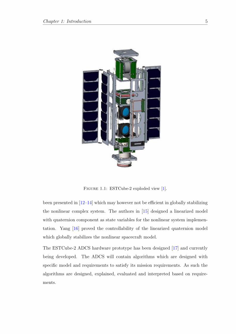
Figure 1.1: ESTCube-2 exploded view [1].
been presented in [12–14] which may however not be efficient in globally stabilizing
the nonlinear complex system. The authors in [15] designed a linearized model
with quaternion component as state variables for the nonlinear system implemen-
tation. Yang [16] proved the controllability of the linearized quaternion model
which globally stabilizes the nonlinear spacecraft model.
The ESTCube-2 ADCS hardware prototype has been designed [17] and currently
being developed. The ADCS will contain algorithms which are designed with
specific model and requirements to satisfy its mission requirements. As such the
algorithms are designed, explained, evaluated and interpreted based on require-
ments.

Chapter 1: Introduction 6
1.3 Aim and Objectives
The long term goal and objective of this current study is to give a comprehensive
review of ESTCube-2 project relating to spacecraft dynamics and implementation
using quaternions as well as controllers to be used on the satellite for attitude con-
trol. Spacecraft attitude control system is defined herein as consisting of sensors,
attitude actuators and processor which houses the controllers for effective attitude
maneuvers. This study will outline the following sub-objectives:
• An overview of the fundamentals in attitude determination and control
• Explain concepts of different reference frame sensors and actuators used
• To derive mathematically the kinematics and dynamics of the satellite
• Elucidate basic attitude control requirements.
The results gotten from this study will be of great significance to the industry
practitioners as well as other students involved in ESTCube project.
1.4 Thesis Outline
The rest of the thesis is described as follows
• Chapter 2 presents the background to spacecraft attitude control, dis-
cussing reference frames used in spacecraft attitude determination and con-
trol as well as discussing parameters used in attitude representation. Brief
discussion on the sensors and actuators used on ESTCube-2 is also presented
here.
• Chapter 3 presents the satellite model describing the satellite dynamics
and kinematics as well as its linearized model. Environmental disturbance
torques are also discussed as it affects the ESTCube-2 satellite.

Chapter 1: Introduction 7
• Chapter 4 describes in detail the attitude controllers designed based on the
attitude control modes and the set requirements
• Chapter 5 presents the simulation results of the controllers designed based
on specifications and provides analysis.
• Chapter 6 includes the conclusion of the thesis and future work to improve
the controllers designed.
• Appendix D Abstracts based on the work done in this thesis accepted for
oral presentation at 68th International Astronautical Congress to be held
from 25-29 September 2017 in Adelaide, Australia and at the 6th Interplan-
etary CubeSat Workshop to be held on 30-31 May 2017 at Cambridge, UK.

2 Background to Spacecraft
Attitude Control
2.1 Introduction
Spacecraft attitude control system typically consists of sensors, attitude actuators
and processor which houses the controllers for effective attitude maneuvers. In
this chapter, I will give an overview of the fundamentals in attitude determination
and control, thus explaining concepts as the different reference frames, sensors and
actuators used.
2.2 Reference Frame
In Aerospace related applications, many reference frames are used to represent
various rotations and concepts, however for the purpose of this report, I will give
a brief description of the most important reference frames used in the satellite
representations.
8

Chapter 2: Reference Frame 9
2.2.1 Earth-Centered Inertial Reference Frame (ECIF)
The Earth-Centered Inertial Reference Frame (ECIF) is centered in the Earth’s
center. It is a non rotating reference frame that employs the Newton’s laws of mo-
tion and gravity on the spacecraft. For inertial pointing spacecrafts, this reference
frame is quite important in for use. The x-axis points toward the point where the
plane of the Earth’s orbit toward Sun, crosses the Equator going from South to
North, z-axis points toward the North pole and y-axis completes the right hand
Cartesian coordinate system.
2.2.2 Earth-Centered Earth Fixed Reference frame (ECEF)
The Earth-Centered Earth Fixed Reference frame (ECEF) has its origin at the
center of the Earth. The x-axis is the direction axis pointing towards the inter-
section between the Greenwich Meridian and the Equator which is at 0o longitude
and 0o latitude. The z-axis is the direction from the center of the Earth pointing
to the north pole. The y-axis is the direction that completes the right handed
system.
2.2.3 Local-Vertical Local-Horizontal Reference frame (LVLH)
The Local-Vertical Local-Horizontal Reference frame or Orbit frame is most de-
sired for use by many satellites as the z-axis direction points towards the center
of the Earth which is a desired nadir pointing mode of satellites. The origin of
orbit frame coincides with the center of mass of the satellite. The x-axis is in the
direction of the spacecrafts’ motion and is perpendicular to the z-axis. The y-axis
completes the right handed system.
2.2.4 Spacecraft Body Reference frame (SBRF)
The Spacecraft Body Reference Frame has its origin from the centre of mass of
the satellite. In this reference frame, the x-axis is orthogonal to the z-axis and the

Chapter 2: Euler Angles 10
y-axis completes the right-handed orthogonal coordinate reference system.During
the nadir pointing phase of the satellite, the SBRF and the LVLH reference frames
are assumed to be aligned with each other without a rotation about the z-axis.
2.3 Attitude Parameterization
2.3.1 Direction Cosine Matrix (DCM)
The DCM represents the attitude in a 3×3 transformation matrix. This is de-
scribed by the vector dot product between two coordinate axes representing the
cosine of the deviation in angle.
A =
u · x u · y u · z
v · x v · y v · z
w · x w · y w · z
(2.1)
This DCM is not directly applicable in space missions in representations of attitude
as deviations between two coordinate systems is not directly visible or applied to
attitude calculations or representations. The Euler angle described next is more
applicable.
2.3.2 Euler Angles
The Euler angle representation describes one coordinate frame to another in three
successive rotations. This implies a multiplication of three rotation matrices ob-
tained from rotations about three fixed axes. These successive rotations are define
as roll, pitch and yaw, where the roll angle ρ is a rotation about the x-axis, the
pitch angle θ about the y-axis and the yaw angle ψ about the z-axis. The rotation
matrices are defined as follows
The rotation (axis transformation) matrices are given as:

Chapter 2: Quaternions 11
Rz =
cosψ sinψ 0
− sinψ cosψ 0
0 0 1
(2.2)
Ry =
cos θ 0 − sin θ
0 1 0
sin θ 0 cos θ
(2.3)
Rx =
1 0 0
0 cosφ sinφ
0 − sinφ cosφ
(2.4)
Rz is the transformation matrix for a fixed point about the z axis.
Ry is the transformation matrix for a fixed point about the y axis.
Rx is the transformation matrix for a fixed point about the x axis.
The resultant transformation matrix from inertial to body frame is given as
R = Rz.Ry.Rx
R =
cosψ sinψ 0
− sinψ cosψ 0
0 0 1
cos θ 0 sin θ
0 1 0
− sin θ 0 cos θ
1 0 0
0 cosφ − sinφ
0 sinφ cosφ
R =
Cθ.Cψ Cψ.Sθ.Sφ− Cφ.Sψ Cψ.Sθ.Cφ− Sφ.Sψ
Cθ.Sψ Sψ.Sθ.Sφ− Cφ.Cψ Sψ.Sθ.Cφ− Sφ.Cψ
−Sθ Cθ.Sφ Cφ.Cφ
(2.5)
The elements C() and S() are used as an abbreviation for the trignonmetric ex-
pression cos() and sin() respectively.

Chapter 2: Quaternions 12
2.3.3 Unit Quaternions
Quaternions are referred to as hyper complex numbers and was first introduced
by mathematician Rowan Hamilton in the early 19th century and over time have
been applied to mechanics solutions. Quaternions are used to express a rotation by
a rotational angle about an axis unlike Euler angles which represents rotations by
a series of rotations about x, y or z axes. The rotation performed by quaternions
are not explicitly about an x, y or z axes. Just like complex numbers, quaternions
have basis i, j, k satisfying the following expression
i2 = j2 = k2 = −1 = ijk (2.6)
Therefore we can define quaternions as follows representing an addition of both
scalar and vector component.
q = iq1 + jq2 + kq3 + q0 (2.7)
Thus quaternions contains four numbers and for simplicity in expressions, q0 is
the scalar part of the quaternions and the vector component is represented as
qv = iq1 + jq2 + kq3 (2.8)
The normalized quaternion is therefore represented as
q0 = cos(θ/2) (2.9)
qv = esin(θ/2) (2.10)
where
• e is the rotational axis,

Chapter 2: Quaternions 13
• θ is the angle of rotation.
The author in [18] defined and derived the multiplication of two quaternions in
order to obtain the quaternion rotation as follows
a⊗ b = a0b0 − avbv + a0bv + b0av + a× b (2.11)
In recall of complex conjugates, the quaternion complex conjugate can be repre-
sented as
q∗ = q0 − qv = q0 − iq1 − jq2 − kq3 (2.12)
Therefore the norm of a quaternion can then be defined easily as
‖q‖ =√q∗ ⊗ q (2.13)
‖q‖ =√q20 + q21 + q22 + q23 = 1 (2.14)
The inverse of a normalized quaternion satisfying the above equation is
q−1 = q∗ (2.15)
2.3.4 Quaternion Rotation
In order to obtain the quaternion rotation operator, we make use of the normalized
quaternion defined in Equations 2.9 and 2.10. Therefore we express the quaternion
as
q = q0 + qv = cos(θ
2) + esin(
θ
2) (2.16)
and perform quaternion products in order to obtain the rotations.
By defining two quaternions as p = cos(α2) + esin(α
2) and q = cos(β
2) + esin(β
2) we
obtain the quaternion product as follows.

Chapter 2: Quaternions 14
r = p⊗ q =
(cos(
α
2) + esin(
α
2)
)⊗(cos(
β
2) + esin(
β
2)
)(2.17)
r = cos(α + β
2
)+ esin
(α + β
2
)= cos(γ) + esin(γ) (2.18)
The product of two quaternions as seen above represents the two consecutive
rotations by α and β. Equation 2.19 represents the rotation of a quaternion and
a vector v
q ⊗ v = (q0 + qv)⊗ (0 + v) = −qv · +q0v + q × v (2.19)
However, multiplying this expression by the conjugate of the quaternion q∗ gives
the expression in Equation 2.20 which is a vector and expressed further in the
form of direction cosine matrix in Equation 2.21
w = q ⊗ v ⊗ q∗ =
(cos2
(α2
)− sin2
(α2
))v + 2(qv · v)qv + 2q0(qv × v) (2.20)
w1
w2
w3
=
2q0
2 − 1 + 2q12 2q1q2 − 2q0q3 2q1q3 + 2q0q2
2q1q2 + 2q0q3 2q22 − 1 + 2q0
2 2q2q3 − 2q0q1
2q1q3 − 2q0q2 2q2q3 − 2q0q1 2q32 − 1 + 2q0
2
v1
v2
v3
(2.21)
the DCM above can also be defined as a general rotational matrix
C = (2q02 − 1)v + 2(q.v)q + 2q0(q × v) (2.22)
2.3.5 Error Quaternion
The error quaternion is defined as the rotational quaternion between two rotations.
The error quaternion is obtained by quaternion product of the inverse quaternion

Chapter 2: Sensors 15
representing the desired quaternion of one point to another and the initial quater-
nion itself, given below
qe = q−1d ⊗ q (2.23)
qe =
qd0 qd1 −qd2 −qd3−qd1 qd0 qd3 −qd2qd2 −qd3 qd0 −qd1qd3 qd2 qd1 qd0
q0
q1
q2
q3
(2.24)
The quaternion error qe satisfies the unit quaternion constraint.
2.4 Sensors
The sensors used in the ADCS of ESTCube-2 include gyroscopic sensors, ac-
celerometers, magnetometers, Sun sensors, and star tracker [19]. These were se-
lected in order to be able to meet the pointing requirements and accurately obtain
the attitude beyond LEO.
2.4.1 Gyroscopes
The satellite will consist of 4 gyroscopic sensors which have been selected and
tested on a prototype sensor board.
2.4.2 Accelerometers
Two accelerometers will be used on the satellite mainly for closed loop control of
the cold gas thrusters.

Chapter 2: Actuators 16
2.4.3 Magnetometers
The satellite will contain two Magnetometers which will be used mainly for attitude
determination in LEO.
2.4.4 Sun sensor
On board the satellite will be 6 sun senors which are developed in house. Though
the sun sensors provide less accuracy than star tracker, they are required for more
frequent measurements.
2.4.5 Star tracker
The star tracker is a separate subsystem and will be used to obtain very accurate
and precise attitude information in combination with other sensors even during
the satellite spin up.
2.5 Actuators
2.5.1 Reaction Wheels
Reaction wheels are actuators that provide fine attitude control which results from
the acceleration of the flywheel. The rotational acceleration is as a result of an
electric motor which could output a varied rotation. The control Torque produced
is opposite to the rate of change of angular momentum of the wheel as given in
the Equation.
Tc = −J · w = −H (2.25)
where
• Tc is control torque generated.
Chapter 2: Actuators 17
• J is the moment of inertia.
• w is the angular velocity vector.
• H is the angular momentum of the wheel.
The reaction wheels cannot be used exclusivelsy as there is a build up in angular
momentum of the wheels which mskes it saturated. As such, the ACS also makes
use of the thrusters and magntic coils which will be used to generate external
torque to unsaturate the angular momentum in the wheels. The reaction wheels
used on ESTCube-2 has a momentum storage of 1.5mNms.
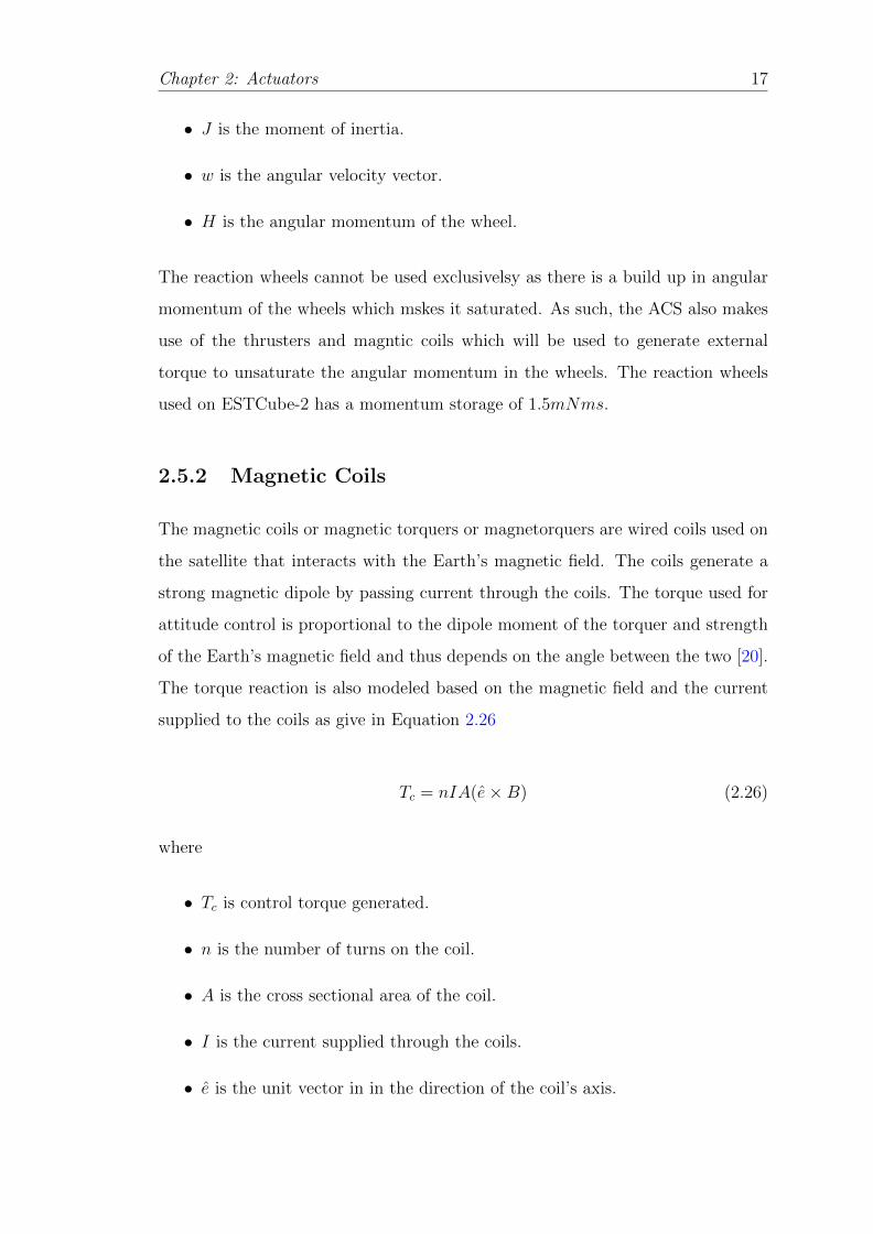
2.5.2 Magnetic Coils
The magnetic coils or magnetic torquers or magnetorquers are wired coils used on
the satellite that interacts with the Earth’s magnetic field. The coils generate a
strong magnetic dipole by passing current through the coils. The torque used for
attitude control is proportional to the dipole moment of the torquer and strength
of the Earth’s magnetic field and thus depends on the angle between the two [20].
The torque reaction is also modeled based on the magnetic field and the current
supplied to the coils as give in Equation 2.26
Tc = nIA(e×B) (2.26)
where
• Tc is control torque generated.
• n is the number of turns on the coil.
• A is the cross sectional area of the coil.
• I is the current supplied through the coils.
• e is the unit vector in in the direction of the coil’s axis.

Chapter 2: Actuators 18
The magnetorquers for ESTCube-2 are a similar design to those of ESTCube-1
[17]. For ESTCube-2, the area of the magnetoquers were increased based on the
size of the 3U satellite and the demand for a larger magnetic torque. The magnetic
moment of the magnetorquer is 0.5 A/m2 in the three axis.
2.5.3 Cold Gas Thruster
Thrusters are mostly used in spacecraft in higher altitudes outside the significant
influence of the Earth’s magnetic field. They are needed for large attitude maneu-
vers. The thruster to be used on ESTCube-2 is the cold gas thruster developed
by Nanospace AB and includes four thrust nozzles in the same -z axis direction.
The nominal thrust is 1mN and the torque created is a product of the thrust and
the distance to the centre of mass. More description on application of pulse width
modulation on thrusters with control laws is given in [21].

3 Spacecraft Modeling
In this Chapter, I will describe the satellite dynamics with mathematical models
and disturbances with view of obtaining an approximate linearized model for the
satellite for controller implementation.
3.1 Kepler And Newton’s Laws
The motion of celestial bodies have been studied and laws postulated by Johannes
Kepler based on works of Tycho Brahe [22] [21]. With respect to orbital evaluation
of two point masses, a model for a spacecraft orbiting a planet can be obtained
be considering equations of motions and Newton’s second law. Kepler postulated
the following laws which apply to satellite motion in Earth’s orbit
• The orbit of each planet is an ellipse, with the Sun at one focus.
• The radius vector drawn from the planet to the Sun sweeps out equal areas
in equal times.
• The square of the period of a planet is proportional to the cube of its mean
distance from the Sun.
These laws corresponds and also applies to spacecraft motion in Earth orbit, where
the Sun represents the Earth and the planet represent the spacecraft in orbit.
19
Chapter 3: Inertia Matrix 20
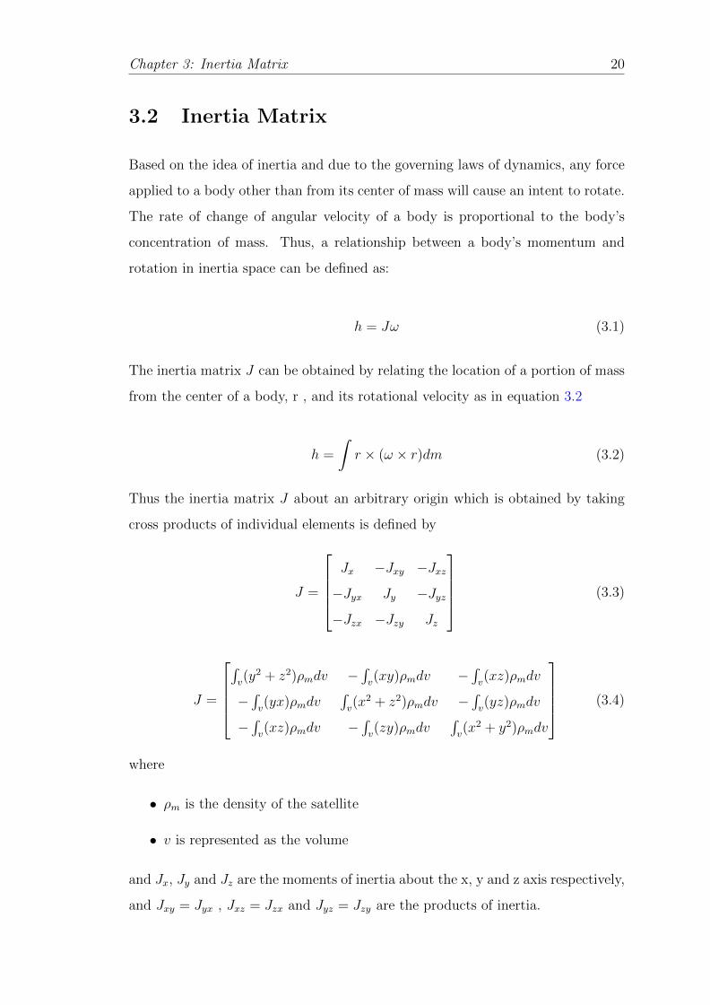
3.2 Inertia Matrix
Based on the idea of inertia and due to the governing laws of dynamics, any force
applied to a body other than from its center of mass will cause an intent to rotate.
The rate of change of angular velocity of a body is proportional to the body’s
concentration of mass. Thus, a relationship between a body’s momentum and
rotation in inertia space can be defined as:
h = Jω (3.1)
The inertia matrix J can be obtained by relating the location of a portion of mass
from the center of a body, r , and its rotational velocity as in equation 3.2
h =
∫r × (ω × r)dm (3.2)
Thus the inertia matrix J about an arbitrary origin which is obtained by taking
cross products of individual elements is defined by
J =
Jx −Jxy −Jxz−Jyx Jy −Jyz−Jzx −Jzy Jz
(3.3)
J =
∫v(y2 + z2)ρmdv −
∫v(xy)ρmdv −
∫v(xz)ρmdv
−∫v(yx)ρmdv
∫v(x2 + z2)ρmdv −
∫v(yz)ρmdv
−∫v(xz)ρmdv −
∫v(zy)ρmdv
∫v(x2 + y2)ρmdv
(3.4)
where
• ρm is the density of the satellite
• v is represented as the volume
and Jx, Jy and Jz are the moments of inertia about the x, y and z axis respectively,
and Jxy = Jyx , Jxz = Jzx and Jyz = Jzy are the products of inertia.

Chapter 3: Environmental Models 21
If the principal axes of inertia coincide with the axes of the body frame by being
symmetric with its axes Jxy = Jxz = Jyz = 0, the inertia matrix reduces to:
J =
Jx 0 0
0 Jy 0
0 0 Jz
(3.5)
3.3 Environmental Models
This section will discuss and examine the environmental torque models. Spacecraft
in orbit are subjected to a variety of environmental torques which affect its atti-
tude. These could be either internal disturbance torques caused by the spacecraft
or external environmental disturbances. The main disturbances to be evaluated
will be magnetic disturbance torque, solar radiation pressure torque, aerodynamic
torque and gravity-gradient torque and how much of influence they will have on
ESTCube-2 considering the satellite in LEO and GEO. A disturbance torque based
on the thruster axis misalignment will also be discussed and evaluated based on
some values of misalignment.
3.3.1 Earth’s Geomagnetic Field
Spacecrafts in LEO are greatly influenced by Earth’s magnetic field. Hence appli-
cation of magnetic control laws is dependent on the Earth’s magnetic field. The
geomagnetic field is extensively described in [23], a brief description of its model
and effect on spacecraft is discussed here. The geomagnetic field can be modeled
as a magnetic dipole which is tilted about 11.5 deg with the magnetic south near
the geographical north pole and the magnetic north, near the geographical south
pole as seen in Figure 3.1.
The geomagnetic field is much higher at altitudes closer to the Earth and decrease
with an increase in altitude. The magnetic field strength at the equator is approx-
imately 0.03mT [2] and as seen in Figure 3.1, lines are closer at the poles hence a

Chapter 3: Environmental Models 22
Figure 3.1: Earth’s Magnetic Dipole [2].
stronger magnetic force experienced at the poles approximately twice the strength
to that at the equator.
The International Geomagnetic Reference Field (IGRF) is a standard geomagnetic
model used to describe the Earth’s magnetic field. The IGRF models entails a lot
of computation, however estimates of the Earth’s magnetic field are done using a
dipole model. Controllers are also designed based on the dipole model as effective
designs can be made with regards errors in magnetic field measurements. The
dipole model which will be used later in this work in the design of linear quadratic
regulator is mathematically defined as [24]
b =
b1(t)
b2(t)
b3(t)
=µfa3
cosω0t sin θ
− cos θ
2 sinω0t sin θ
(3.6)
where θ is the inclination with respect to the geomagnetic equator, a is the orbit’s
semi major axis, ω0 is the orbit angular velocity and µf is the magnetic field’s

Chapter 3: Environmental Models 23
dipole strength in Wb ·m.
3.3.2 Gravity-Gradient Torque
Gravity-gradient disturbance is a torque felt by an Earth orbiting satellite due
to the gravitational force between the earth and the satellite. The Earth’s non-
uniform gravitational field which according to Newton is inversely proportional
to the square of the distance to the Earth causes this torque and also causes the
satellite to obey Kepler’s law of planetary motion as described in 3.1 The gravity-
gradient torque on a body is derived as
Tg =3µ
2Rs
3
|Rs × (J · Rs)| (3.7)
where
• µ is the gravitational constant of the earth.
• Rs is a vector representing the distance from the center of the earth to the
satellite.
• J is the moment of inertia tensor of the satellite as described in 3.2.
Equation 3.7 could be used to obtain a detail analysis and also obtain the torques
about each axis when the body frame is along the reference frame. However a
more simplified equation is presented in [25] is used in this report based on the
maximum gravity gradient disturbance torque.
Tg =3µ
2R3 s|Jz − Jy| sin(2θ) (3.8)
where Tg is the maximum gravity torque, Jz and Jy are the largest and smallest
moment of inertia, and θ is the maximum deviation from the local vertical.
Based on the formula given in 3.2 and a satellite mass of about 4kg, the moments
of inertia about the x, y and z axes are calculated to be 0.0333kg.m2, 0.0333kg.m2
and 0.0067kg.m2 respectively.
Chapter 3: Environmental Model 24
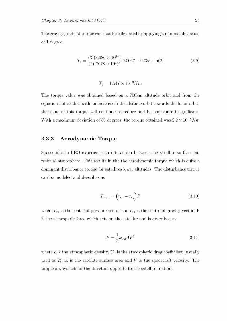
The gravity gradient torque can thus be calculated by applying a minimal deviation
of 1 degree:
Tg =(3)(3.986× 10¹⁴)
(2)(7078× 103)3|0.0067− 0.033| sin(2) (3.9)
Tg = 1.547× 10⁻⁹Nm
The torque value was obtained based on a 700km altitude orbit and from the
equation notice that with an increase in the altitude orbit towards the lunar orbit,
the value of this torque will continue to reduce and become quite insignificant.
With a maximum deviation of 30 degrees, the torque obtained was 2.2× 10⁻⁸Nm
3.3.3 Aerodynamic Torque
Spacecrafts in LEO experience an interaction between the satellite surface and
residual atmosphere. This results in the the aerodynamic torque which is quite a
dominant disturbance torque for satellites lower altitudes. The disturbance torque
can be modeled and describes as
Taero =(rcp − rcg
)F (3.10)
where rcp is the centre of pressure vector and rcg is the centre of gravity vector. F
is the atmosperic force which acts on the satellite and is described as
F =1
2ρCdAV
2 (3.11)
where ρ is the atmospheric density, Cd is the atmospheric drag coefficient (usually
used as 2), A is the satellite surface area and V is the spacecraft velocity. The
torque always acts in the direction opposite to the satellite motion.

Chapter 3: Dynamics 25
3.3.4 Solar Radiation Torque
The solar photons which impact on the surface of the satellite creates a force which
produces a torque about the centre of mass of the satellite. The force acting on
the satellite depends on if the incident radiation is absorbed or reflected. The
torque is independent of the altitude of the satellite. The solar radiation torque is
modeled as
Ts =(rcp − rcg
)F (3.12)
where F is
F =FscA(1 + q) cos i
Fs is the solar constant (1371W/m2), c is the speed of light (3× 10⁸m/s), A is the
surface area, q is the reflectant coefficient ranging between 0 and 1, i is the angle
of incidence of the sun.
3.3.5 Residual Magnetic Torque
As experienced by satellites in LEO as well as in ESTCube-1 [26], a magnetic field
is created in the satellite. While the satellite being controlled by the magnetic coils
interacts with Earth’s magnetic field, a magnetic field in the satellite is created
by electric components and other ferromagnetic materials. This magnetic field
is considered as a disturbance as it has an effect on the control of the satellite’s
attitude. The strength of this magnetic field and its direction cannot be easily
determined before launch of the satellite, however measuring and calculating this
residual magnetic torque is needed in other to augment for the disturbance in the
design of the magnetic control laws. The residual magnetic torque can also be
expressed the same way as the magnetorquers described in Section 2.5.2
τres = mres ×B (3.13)
In ESTCube-1, the residual magnetic moment was the dominant disturbance
torque in the satellite and it was estimated as 0.1Am2 [27]

Chapter 3: Dynamics 26
3.4 Dynamics
As mentioned earlier, the quaternion based model has advantages in space tech-
nology applications over the Euler angle representations. The spacecraft dynamics
model has been derived in several texts and here it is reviewed and simplified. In
order to derive the dynamic model of the satellite, the satellite is assumed to act
as a rigid body as well as a point mass in orbit. Hence Newton-Euler formulation
is used where the angular momentum relates to the applied torque.
By application of Newton’s second law to the spacecraft’s rotational motion
M = hi (3.14)
where
• h is the angular momentum
• M is the applied torque or external moment in inertial frame with reference
to body frame
in view of coriolis equation [28], (3.14) can be expressed as
M = h+ ωi × h (3.15)
therefore, the rate of angular momentum can be defined as
h = Jωi = −ωi × Jωi +M (3.16)
M can be expressed as addition of all disturbance torques and a control torque Tc
Jωi = Td + Tc − Ω(ωi)Jωi (3.17)
where

Chapter 3: Kinematics 27
• Ω(ωi) is the skew symmetric representation of the angular velocity in inertial
reference frame.
Ω(ωi) =
0 −ω1 −ω2 −ω3
ω1 0 ω3 −ω2
ω2 −ω3 0 ω1
ω3 ω2 −ω1 0
(3.18)
• Td is the sum of disturbance torques acting on the satellite
• Tc is the applied control input torque
The varying torques acting on the satellite changes with respect to the selection
of actuator for specific attitude operation.
3.5 Kinematics
The kinematic model describes the orientation of the satellite by integrating the
angular velocity. The kinematic differential equations represented in quaternions
as derived in [23]
q = −1
2ω × qv +
1
2qoω (3.19)
q0 = −1
2ωT qv (3.20)
The quaternion representation that rotates body frame in relation with the refer-
ence frame is
q =[qo, q
Tv
]T=[cos(α
2), eT sin(α
2)]T
(3.21)
where we define the rotational axis by a unit vector e and the angle of rotation
around that axis by α. The vector qe described by eT sin(α2) = [q1, q2, q3]
T and the

Chapter 3: Linearization 28
scalar component of the quaternion by qo = cos(α2). Thus from (3.19), we obtain
q0
q1
q2
q3
=1
2
0 −ω1 −ω2 −ω3
ω1 0 ω3 −ω2
ω2 −ω3 0 ω1
ω3 ω2 −ω1 0
q0
q1
q2
q3
=1
2
q0 −q1 −q2 −q3q1 q0 −q3 q2
q2 q3 q0 −q1q3 −q2 q1 q0
0
ω1
ω2
ω3
(3.22)
The vector component can be easily obtained from the property of quaternion
given in section 2.3 q0 =√
1− q21 − q22 − q23q1
q2
q3
=1
2
q0 −q3 q2
q3 q0 −q1−q2 q1 q0
ω1
ω2
ω3
(3.23)
3.6 Linearization
The satellite model equations as given in 3.17 and 3.23 represents the non linear
dynamics and kinematics models. In order to use these equations for an optimal
controller such as the Linear Quadratic Controller, these nonlinear equations have
to be linearized.
The linear form of the satellite attitude equations can be obtained by linearizing
the equations about an equilibrium or stationary point. The linearization points
based on a first order Taylor expansion about the stationary point are selected
and given as in 3.24
q =[1, 0]T
(3.24)
Equation 3.23 can be represented as a function
qv = g(q, ωi) (3.25)

Chapter 3: Linearization 29
therefore a partial derivative will be represented as
qv =∂g
∂q(q) +
∂g
∂ωi(ωi) (3.26)
linearizing with change around the equilibrium point e, assume at equilibrium we
have stationary point where q1 = q2 = q3 = 0 and ωi = 0.
qv − qe =∂g
∂q(q − qe) +
∂g
∂ωi(ωi − ωie) (3.27)
expanding equation 3.23 yields the following equations
q1 =1
2(q0ω1 − q3ω2 + q2ω3) (3.28)
q2 =1
2(q3ω1 + q0ω2 − q1ω3) (3.29)
q3 =1
2(−q2ω1 + q1ω2 + q0ω3) (3.30)
with respect to equation 3.27, the above equations 3.28, 3.29 and 3.30 becomes
q1 = 0− 0 + 0 +1
2(q0)− 0 + 0 (3.31)
q2 = 0 + 0− 0 + 0 +1
2(q0) + 0 (3.32)
q3 = −0 + 0 + 0− 0 + 0 +1
2(q0) (3.33)
Therefore the matrix representation is expressed as

Chapter 3: Linearization 30
q1
q2
q3
=
0 0 0 1
2(q0) 0 0
0 0 0 0 12(q0) 0
0 0 0 0 0 12(q0)
q1
q2
q3
ω1
ω2
ω3
(3.34)
qv =[03
12(I3)
]qvωi
(3.35)
where q0 = 1 at equilibrium.
Also by performing the expansion and linearization of 3.17 and assuming the
approximation with negligible disturbance torque.
Jωi ≈ Tc (3.36)
qvωi
=
0312(I3)
03 03
qvωi
+
03
J−1
(Tc) (3.37)
= Ax+Bu (3.38)
where u represents the control input Tc and
A =
0312(I3)
03 03
, x =
qvωi
, B =
03
J−1
(3.39)

4 Attitude Control for
ESTCube-2
4.1 Description and Control Specifications for
ESTCube-2
Based on the mission objectives for ESTCube-2, the centrifugal deployment of E-
sail Tether requires enough angular momentum, as such the control design should
spin up the satellite to one revolution per second (360 deg/s). For this purpose, the
satellite spin axis must be aligned with the Earth’s polar axis with pointing error
of less than 3 degrees [27]. Also for ground station pointing and Earth observation,
the pointing accuracy should be less that 0.1 degrees.
4.2 Detumbling Controller Designs
The purpose of the detumbling mode is to detumble or stabilize the angular rate of
the satellite after orbital insertion or release from the launch vehicle and to ensure
that the satellite can be in a controllable state. The controller designed for this
mode must be able to regain control of the satellite in situations where control of
the satellite has been lost. In general, the kinetic energy of the satellite is reduces,
thus causing a reduction in the angular velocity of the satellite for optimal control.
31

Chapter 4: Attitude Control Designs 32
The controller used in this mode is selected because the commanded magnetic
dipole moment can be obtained directly from the calculations and is used as an
input for the actuator. Also, the magnetometer measurement can always be read
and used for the control algorithm
4.2.1 B-dot Controller Design
The B-dot controller had been specifically chosen for detumbling of the satellite.
This is in view of the fact that it only requires the derivative of the magnetic field
as input making it the best choice in terms of efficiency even when other orbital
parameters could be missing.
The B-dot is derived by observing a decrease in the rotational energy during
detumbling. This basically means that the scalar product of the angular velocity
and the control torque must be negative
ωTi · τ < 0 (4.1)
where τ is represented as the control torque delivered by magnetic actuator and
is expressed as
τ = m×B (4.2)
where m is the commanded magnetic dipole moment and B is the geomagnetic
field vector. A seemingly accurate model of the geomagnetic field for LEO circular
orbit such as IGRF is being used as the model for the simulation.
the condition in equation 4.1 then becomes
ωTi · (m×B) < 0 (4.3)
Applying cross product rules given in section 2.3, the condition in 4.3 can be
rewritten as
Chapter 4: Attitude Control Designs 33
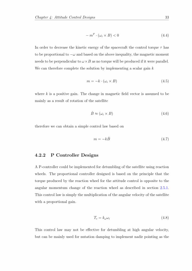
−mT · (ωi ×B) < 0 (4.4)
In order to decrease the kinetic energy of the spacecraft the control torque τ has
to be proportional to −ω and based on the above inequality, the magnetic moment
needs to be perpendicular to ω×B as no torque will be produced if it were parallel.
We can therefore complete the solution by implementing a scalar gain k
m = −k · (ωi ×B) (4.5)
where k is a positive gain. The change in magnetic field vector is assumed to be
mainly as a result of rotation of the satellite
B ≈ (ωi ×B) (4.6)
therefore we can obtain a simple control law based on
m = −kB (4.7)
4.2.2 P Controller Designs
A P-controller could be implemented for detumbling of the satellite using reaction
wheels. The proportional controller designed is based on the principle that the
torque produced by the reaction wheel for the attitude control is opposite to the
angular momentum change of the reaction wheel as described in section 2.5.1.
This control law is simply the multiplication of the angular velocity of the satellite
with a proportional gain.
Tc = kωωi (4.8)
This control law may not be effective for detumbling at high angular velocity,
but can be mainly used for nutation damping to implement nadir pointing as the

Chapter 4: Attitude Control Designs 34
maximum torque generated with the reaction wheel is 0.0001Nm and hence will
require unloading upon saturation of the reaction wheels.
4.2.3 PD Controller Designs
The PD controller designed is an implementation of the magnetic control law as
defined in equation 4.2. The control law makes use of the magnetic field vector and
the angular velocity and attitude of the satellite. The PD control implemented
here is a simple controller model used for both magnetic coils and reaction wheels.
While this control law attenuates the initial angular velocities, it also keeps the
quaternion attitude at zero for all three axes. This control law makes use of
calculated error vector to determine the most favourable magnetorquing moment
for use with the magnet torquers. This is then utilized directly as the required
torque vector. The error vector is composed of the quaternion error and the
angular velocity in the body axes.
~e = kω(ωi ×B) + kq(qe ×B) (4.9)
where B is the magnetic field vector. Kω and Kq are the controller gains which
are chosen based on the performance of several tests of the system. qe is the
quaternion error defined as
qe =
qd0 qd1 −qd2 −qd3−qd1 qd0 qd3 −qd2qd2 −qd3 qd0 −qd1qd3 qd2 qd1 qd0
q0
q1
q2
q3
(4.10)
4.3 Pointing Controller Designs
The controllers designed for the pointing mode of the satellite is aimed to satisfy
the requirements specified for pointing [29]. As such a simple PD controller for em-
ployed to both magnetic torquers and reaction wheels is described. Furthermore,
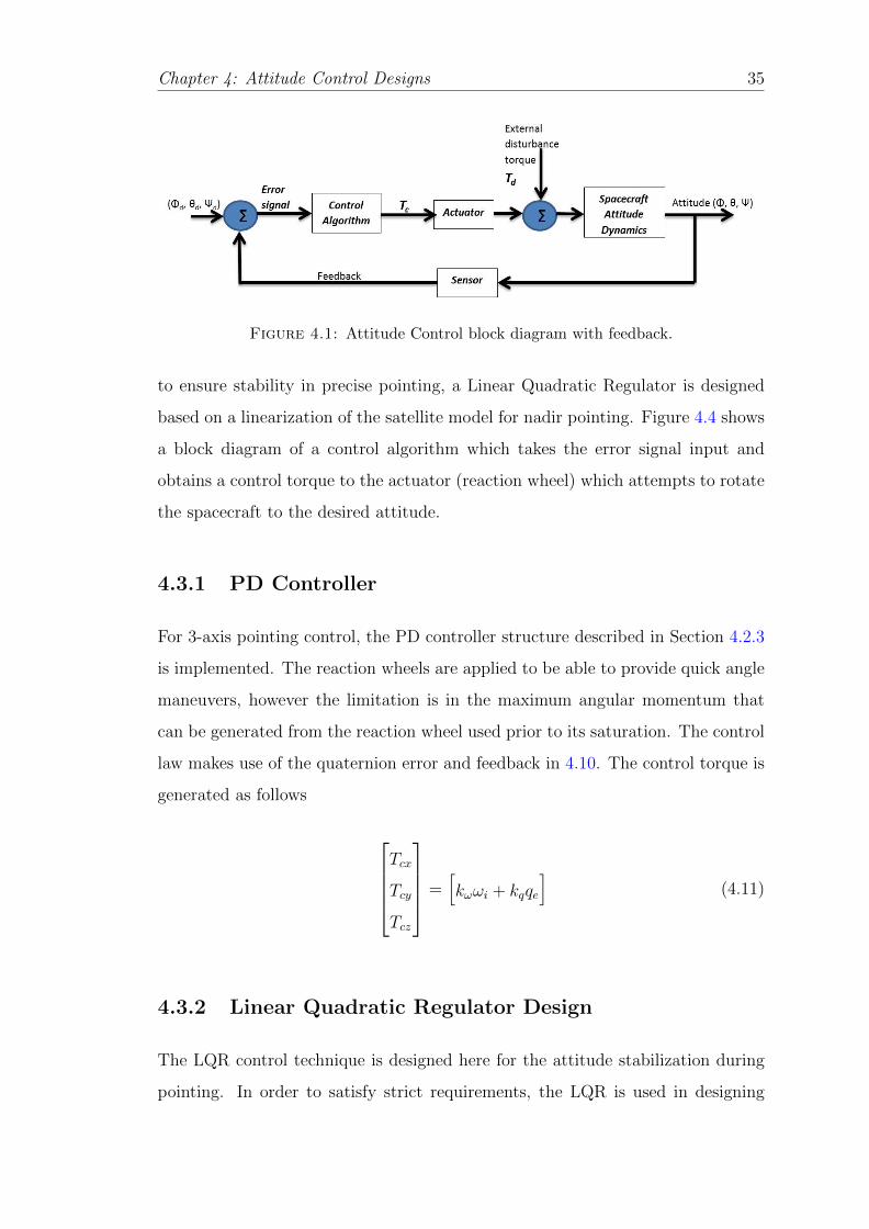
Chapter 4: Attitude Control Designs 35
Figure 4.1: Attitude Control block diagram with feedback.
to ensure stability in precise pointing, a Linear Quadratic Regulator is designed
based on a linearization of the satellite model for nadir pointing. Figure 4.4 shows
a block diagram of a control algorithm which takes the error signal input and
obtains a control torque to the actuator (reaction wheel) which attempts to rotate
the spacecraft to the desired attitude.
4.3.1 PD Controller
For 3-axis pointing control, the PD controller structure described in Section 4.2.3
is implemented. The reaction wheels are applied to be able to provide quick angle
maneuvers, however the limitation is in the maximum angular momentum that
can be generated from the reaction wheel used prior to its saturation. The control
law makes use of the quaternion error and feedback in 4.10. The control torque is
generated as follows
Tcx
Tcy
Tcz
=[kωωi + kqqe
](4.11)
4.3.2 Linear Quadratic Regulator Design
The LQR control technique is designed here for the attitude stabilization during
pointing. In order to satisfy strict requirements, the LQR is used in designing

Chapter 4: Attitude Control Designs 36
linear controllers for such complex non linear systems like the CubeSat. The
design aims to find a cost function and minimize this cost function.
x = Ax+Bu (4.12)
Based on the linearized satellite model designed for nadir pointing in C with state
space quaternion model given in Equation 4.12, the controller implements a basic
feedback control u for optimization,
u = −Kx (4.13)
where K is the feedback gain matrix calculated to minimize the Linear Quadratic
cost function
J =
∫ ∞0
[xTQx+ uTRu]dt (4.14)
where Q and R are positive definite matrices known as the state weight matrix and
control input weight matrix respectively, where Equation 4.13 is further expressed
as
u = −R−1BTPx (4.15)
where P is a symmetric positive semi-definite solution of the Algebraic Riccati
Equation (ARE) given below
0 = PA+ ATP +Q− PBR−1BP (4.16)
Based on the calculated value for the gain K, |A−BK| must be stable to obtain
a correct and optimal result. For stability it can be analysed that the eigenvalues
must have negative real parts. Hence Equation 4.16 is only solvable if and only if
input matrices A and B is controllable. For controllability analysis see Appendix
A.
The designed LQR controller convergently stabilizes the nonlinear satellite model
by attempting to bring the initial attitude and angular velocity to the minimal

Chapter 4: Attitude Control Designs 37
Figure 4.2: LQR design from linearization.
Figure 4.3: LQR controller on nonlinear spacecraft model.
equilibrium point. At this equilibruim point, the linearised model approximates
the non linear model as efficiently as possible.
The satellite state x is given as
x = [qe1 qe2 qe3 ω1 ω2 ω3]T (4.17)
where qe1 qe2 qe3 can be defined as the quaternion error to obtain the desired
attitude in quaternion for pointing which can be calculated from the quaternion
error defined in 2.3.5.

Chapter 4: Attitude Control Designs 38
Figure 4.4: LQR controller design algorithm.

Chapter 4: Spin-up Controller Designs 39
4.4 Cross Product Control Law
The controllability of the reaction wheels is limited by the saturation of the wheels
unlike the magnetorquers which are subject to the geomagnetic field. To solve this,
several approaches for wheel desaturation and unloading have been discussed and
developed [5, 30–32]. Here a very simple cross product law is implemented to per-
form the pointing of the satellite by constantly. This control algorithm is based on
the reaction wheel PD control law while constantly verifying the angular momen-
tum of the wheel as a feedback. The magnetorquer is enabled in the algorithm
when the angular momentum of the wheel approaches 1.5m.N.m.s as described in
the Equations below
Tcx
Tcy
Tcz
=[kωωi + kqqe
](4.18)
m = − k
(‖B‖)2[B × he] (4.19)
where Tc is the control torque from the reaction wheels, k, kω, kq are gains for the
algorithm, m is the magnetorquer dipole moment vector in SBRF and he is the
angular momentum error of the wheels.
4.5 Spin-up Controller Designs
The spin up control algorithm designed will aim to spin the satellite to achieve an
angular velocity of 360 deg/s. This high spin rate is based on mission requirement
of spinning the satellite to generate enough angular momentum for the centrifugal
deployment of tether for the plasma break experiment [19].
In order to control the spin motion of the satellite, three important control factors
needs to be simultaneously considered. These are spin control, precession control,
nutation control [33]. The spin rate controller designed here makes use of the

Chapter 4: Spin-up Controller Designs 40
magnetorquers based on the strong magnetic field in the LEO environment. As
the ESTCube-2 CubeSat would be used to test algorithms for the ESTCube-3
which is to be launched in Lunar orbit, a spin rate control based on reaction
wheels and cold gas thrusters will also be designed but not covered in the scope of
this thesis. The control law which is based on a Lyapunov like function satisfies
the spin rate and nutation control while aligning the spin axis with Earth’s polar
axis. This is obtained by considering the rate of angular momentum as defined in
Equation 3.17 to be
h = Tc − Ω(ωi)Jωi (4.20)
Here we consider the disturbance torque to be negligible and the angular momen-
tum error to be he = h−hd, therefore the rate of angular momentum error is given
as
he = Tc − Ω(ωi)he (4.21)
Since we desire a spin about the x-axis, we define the angular momentum error
he = 0, then hx = hd. We assume the principal axes of inertia coincide with the
axes of the body frame, therefore Equation 3.5 holds and the angular rates in the
transverse axes be controlled where w2 = w3 = 0. Then we assume Jy = Jz = Jt
and Equation 4.20 becomes
Jxω1
Jtω2
Jtω3
= Tc −
0 −ω3 ω2
ω3 0 −ω1
−ω2 ω1 0
Jxω1
Jtω2
Jtω3
(4.22)
where Jt is the transverse component of the inertia matrix of the satellite and
simplified further to Jxω1
Jtω2
Jtω3
= Tc +
0
(Jt − Jx)(ω1ω3)
(Jx − Jt)(ω1ω2)
(4.23)

Chapter 4: Spin-up Controller Designs 41
Therefore the rate of angular momentum about the spin axis is given as
h1 = Jxω1 = Tc
[1 0 0
](4.24)
and the error is then calculated to be he1 = h1 − hd and error rate therefore is
he1 = Tc
[1 0 0
](4.25)
The control law is then defined based on the time derivative of a Lyapunov function
V defined in [34]
V = (heT + k1he1
[1 0 0
]+ k2ω
TP )Tc (4.26)
and simplified further in the control equation given below for the required spin
rate of the satellite in the x-axis for tether deployment.
m = − k
(‖B‖)2[B × (he + k1he1
1
0
0
+ k2Sω)] (4.27)
where m is the magnetorquer dipole moment vector in SBRF and k, k1, k2 are
control law gains. S represents the axes selection matrix.
This control law and gains needs to be adjusted for the specific implementation
of the tether deployment and ran in an iterative loop sequence. In obtaining
preliminary results for the optimal performance of the controller, the following
points are noted:
• The B-dot algorithm described Section 4.2.1 for detumbling of the satellite
should first be used to reduce the angular momentum of the satellite in order
to improve the performance of the spin up algorithm.
• For the iterative loop in running the controller, the initial desired angular
velocity should be approximately 45 deg/s to ensure stability along the spin
axis.

Chapter 4: Spin-up Controller Designs 42
• The value of the control gains should be set as: k2 > 1, k1 < 1, k >> k1 to
augment the nutation damping process and avoid uncontrolled spinning of
the satellite about the transverse axis.

5 Simulation Results and Controller
Comparison
This section presents results of the controllers designed and their performances to
the system set with varying initial conditions. The attitude control system was
designed and simulated with MATLAB and SIMULINK.
5.1 B-dot Controller Analysis
The results of the control algorithm described in Section 4.2.1 are depicted in
Figures 5.1 to 5.3. The angular velocity components are seen to attain a steady
state with zero error. As evident with magnetic control, the response has a fast
transient and tends to converge at steady state with a very slow response. The
response shown is based on setting the frequency to 100Hz.
5.2 PD Controller Analysis
The PD controllers were tested with several cases while applying varying gains to
determine an optimum performance. The performance overview is presented in
Table 5.1 and result shown in Figures 5.4 to 5.14.
43

Chapter 5: Simulation Results 44
Figure 5.1: Detumbling of Satellite with Bdot Control
Figure 5.2: Quaternion Attitude during detumbling phase.
5.2.1 PD performance with Magnetorquers
The simulations with the magnetorquers were performed with an initial angular
velocity of (0.05, 0.05, 0.3)rad/s and demonstrate in Figure 5.4 that the proposed
control law achieves attenuating of the satellite angular velocity in approximately

Chapter 5: Simulation Results 45
Figure 5.3: Magnetorquer Torque response during detumbling phase.
Parameters Value UnitOrbit Period To 5400 Sec
Orbit Angular Velocity ωo = 2π/To Rads/sec
Parameters Reaction Wheels MagnetoquersKw 10−3 100Kq 10−2 20000
Initial Angular Velocity (0.1, 0.1, 0.3)rad/s (0.05, 0.05, 0.3)rad/sInitial Quaternion attitude (0, 0, 0, 1) (0, 0, 0, 1)
Table 5.1: PD Performance Overview.
1 orbit. Also the control law begins to maintain a stabilized attitude in approx-
imately 9 orbits in all axes towards nadir pointing. The torque produced is seen
to decline in about 1000secs as the oscillations of the angular velocity begins to
attenuate.
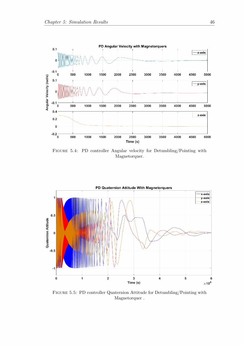
Chapter 5: Simulation Results 46
Figure 5.4: PD controller Angular velocity for Detumbling/Pointing withMagnetorquer.
Figure 5.5: PD controller Quaternion Attitude for Detumbling/Pointing withMagnetorquer .

Chapter 5: Simulation Results 47
Figure 5.6: Magnetorquer Torque response.
Chapter 5: Simulation Results 48
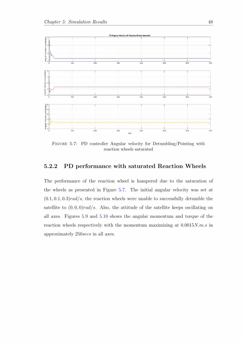
Figure 5.7: PD controller Angular velocity for Detumbling/Pointing withreaction wheels saturated
5.2.2 PD performance with saturated Reaction Wheels
The performance of the reaction wheel is hampered due to the saturation of
the wheels as presented in Figure 5.7. The initial angular velocity was set at
(0.1, 0.1, 0.3)rad/s, the reaction wheels were unable to successfully detumble the
satellite to (0, 0, 0)rad/s. Also, the attitude of the satellite keeps oscillating on
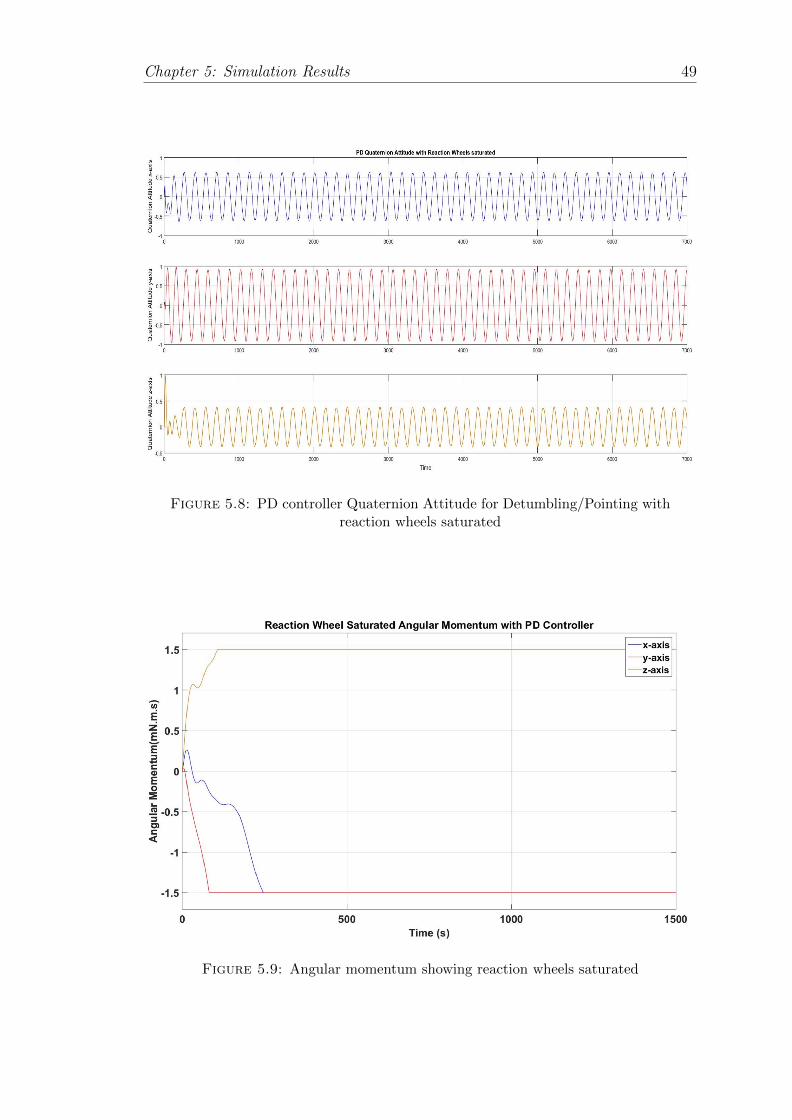
all axes. Figures 5.9 and 5.10 shows the angular momentum and torque of the
reaction wheels respectively with the momentum maximizing at 0.0015N.m.s in
approximately 250secs in all axes.
Chapter 5: Simulation Results 49
Figure 5.8: PD controller Quaternion Attitude for Detumbling/Pointing withreaction wheels saturated
Figure 5.9: Angular momentum showing reaction wheels saturated

Chapter 5: Simulation Results 50
Figure 5.10: Reation Wheel saturated torque response

Chapter 5: Simulation Results 51
Figure 5.11: PD controller Angular velocity for Detumbling/Pointing withreaction wheels
5.2.3 PD performance with unsaturated wheels
The PD control law simulations were tested with the reaction wheels at an initial
angular velocity lowered to (0.04, 0.04, 0.18)rad/s and can be seen that the reaction
wheel does not get saturated with this initial velocity. The satellite as seen in
Figure 5.11 stabilizes to 0 deg in all axes in about 750secs and also maintains
the desired nadir pointing mode in a similar time frame. The angular momentum
and reaction wheel torque response are presented in Figures 5.13 and 5.14with the
angular momentum maintaining a value with magnitude less than 0.0015N.m.s in
all axes.

Chapter 5: Simulation Results 52
Figure 5.12: PD controller Quaternion Attitude for Detumbling/Pointing withreaction wheels
Figure 5.13: Angular momentum showing reaction wheels
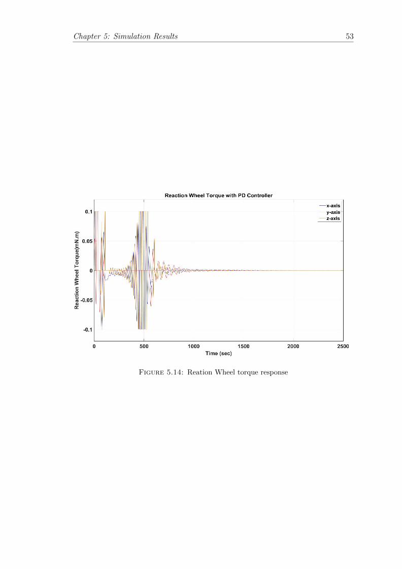
Chapter 5: Simulation Results 53
Figure 5.14: Reation Wheel torque response

Chapter 5: Simulation Results 54
Figure 5.15: Angular velocity response while unloading Reaction Wheels withmagnetorquers
5.3 Cross Product Control Analysis
The Cross product control law simulations were tested with the reaction wheels and
magnetorquers with an initial angular velocity of the satellite (0.1, 0.1, 0.3)rad/s.
The angular velocity of the satellite as seen in Figure 5.15 attenuates to 0 deg in
all axes in about 750secs. The quaternion attitude attempts to stabilize in about
4000secs to nadir pointing mode. The angular momentum of the reaction wheel
as seen in Figure 5.17 saturates in about 100secs and at the same time torque is
delivered by the magnetorquers as seen in Figure 5.19 which in turn desatrurates
the wheels and the performance is then regulated for effective pointing.

Chapter 5: Simulation Results 55
Figure 5.16: Quaternion Attitude during Reaction Wheel unloading withMagnetorquers
Figure 5.17: Reaction Wheels angular momentum saturated and unloadingwith magnetorquers

Chapter 5: Simulation Results 56
Figure 5.18: Reaction Wheel torque response during unloading
Figure 5.19: Magnetorquer torque response with Reaction Wheel unloading

Chapter 5: Simulation Results 57
Parameters Values UnitsSatellite mass 4 KgInertia Matrix Jx = 0.0331, Jy = 0.0331, Jz = 0.00678 Kg m2
Orbit Period To 5400 SecOrbit Angular Velocity ωo = 2π/To Rads/sec
Table 5.2: Satellite Parameters to obtain LQR controller gain.
5.4 LQR Analysis
The feedback control input defined in Equation 4.15 establishes the stability of
the linearized model in a closed loop system while minimizing the cost function
4.14. In order to obtain this control input, the inertia matrix J is calculated and
assumed to be diagonal as expressed in Equation 3.5. For further simplification
of the design process, the weight matrices Q and R are selected to be diagonal
with the number of states and number of actuator control as the lengths Q and R
respectively.
Q = diag[Q1, Q2, Q3, Q4, Q5, Q6]
R = diag[R1, R2, R3] (5.1)
Q and R matrices are selected by adjusting the values and comparing the perfor-
mances to the desired goal using code written in MATLAB where the feedback
gain K is also calculated using the function lqr in MATLAB
[K,P,E] = lqr(A,B,Q,R) (5.2)
where P is the solution of the ARE given in 4.16 and E is the closed loop eigen
values |A−BK| that must guarantee stability.
Figure 5.20 and 5.21 shows the step response of the system states with Q and R
matrices selected as Q = diag[1, 1, 1, 1, 1, 1] and R = diag[1, 1, 1]. The result of
the closed loop Eigen values and the controller gain K are

Chapter 5: Simulation Results 58
Figure 5.20: Quaternion Step response (weighting matrices Q = diag[1,1,1,1,1,1], R = diag[1, 1, 1]) .
Figure 5.21: Angular Velocity Step response (weighting matrices Q =diag[1,1,1,1,1, 1], R = diag[1, 1, 1] ).
E = −0.7070 + 0.0171i,−0.7070− 0.0171i,−0.7068 + 0.0171i,
− 0.7068− 0.0171i,−0.7071 + 0.0002i,−0.7071− 0.0002i
K =
0.9977 0.0000 0.0000 1.4134 0.0000 0.0000
0.0000 1.0000 −0.0000 0.0000 1.4142 −0.0000
−0.0000 −0.0000 0.9977 0.0000 −0.0000 1.4134
The result of the LQR controller with reaction wheels for the purpose of precise
pointing can be seen in Figures 5.22 to 5.24. The angular velocity of the satellite

Chapter 5: Simulation Results 59
Figure 5.22: Angular Velocity LQR controller performance with noise.
Figure 5.23: Quaternion Attitude LQR controller response with noise.
attenuates to zero within 100 seconds with little oscillations due to noise. The
pointing requirement is satisfied as seen with 100 seconds as well.
Figures 5.25 to 5.27 shows results of the LQR controller with magnetorquers. The
angular velocity of the satellite is seen to attain rest at 0 deg/s in all axes in about
1500 seconds. The controller gain was calculated with Q and R matrices selected
as Q = diag[140, 140, 140, 140, 140, 140] and R = diag[2480, 2480, 2480]. The state
space model for this simulation is described in Appendix C.2

Chapter 5: Simulation Results 60
Figure 5.24: Angular Velocity LQR controller performance.
Figure 5.25: Angular Velocity LQR controller performance with Magnetor-quers.

Chapter 5: Simulation Results 61
Figure 5.26: Quaternion Attitude LQR controller response with Magnetor-quers.
Figure 5.27: Magnetorquer Torque response with LQR.

Chapter 5: Simulation Results 62
Parameter ValueInitial Angular Velocity (0, 0, 0)deg/s
k 15000k1 0.01
Desired Angular Velocity k2 Gain57 deg/s 100115 deg/s 1000172 deg/s 1000230 deg/s 1000286 deg/s 5000360 deg/s 5000
Table 5.3: Spin rate simulation result.
5.5 Spin-up Controller Analysis
The Spin-up control simulation results are presented in this section with the desired
ultimate angular rate set to 360 deg/s in the x-axis. As described in Section 4.5
the controller gains were set as shown in Table 5.3.
Figure 5.28 shows the angular rate of the satellite in the x-axis to about 110
deg/s while experiencing a spontaneous nutation effect. Figure 5.29 shows the
angular rate spin up to about 180 deg/s, which is implemented in 2 phases to
avoid a frequent nutation about the traverse axis. Figure 5.30 presents the desired
angular rate which is performed in several phases and achieved in about 27 orbits
as enumerated in Table 5.3

Chapter 5: Simulation Results 63
Figure 5.28: Angular Velocity Spin up to 110 deg/s.
Figure 5.29: Angular Velocity Spin up to 180 deg/s.

Chapter 5: Simulation Results 64
Figure 5.30: Angular Velocity Spin up to 360 deg/s.

6 Conclusion & Future Work
6.1 Conclusion
This thesis presented various attitude controller designs for ESTCube-2 nanosatel-
lite. Table 6.1 gives an overview of the the various designed controllers and progress
made with testing and optimization as at the time of this thesis work. Further
work on these will continue to achieve specific desired requirements for the satellite
mission.
Much work was done on the design of LQR optimal controller for use with the
reaction wheels and magnetorquers. The LQR controller was seen to work well
even with the gravity gradient disturbance torque. However, due to the influence
of the Earth’s magnetic field, the response with magnetorquers was not much
Control Law Attitude Mode Status Future workBdot Detumbling(MT) Designed Gain OptimisationPD Detumbling(MT) DesignedP Detumbling(RW ) Designed
PD Pointing(MT) Designed Gain OptimisationPD Pointing(RW) Designed
Cross Product law Wheel unloading(MT/RW) DesignedLQR Pointing(MT) Designed Gain OptimisationLQR Pointing(RW) Designed
Angular rate control Spin-up(MT) Designed Gain OptimisationAngular rate control Spin-up(MT/RW) Theory Designed Design ControllerAngular rate control Spin-up(RW/Thruster) Theory Designed Design Controller
Table 6.1: Overview of Designed Controllers.
65

66
desirable in comparison with reaction wheels. In comparison with the PD-like
control laws, LQR optimal control gave better results to stabilize the system even
when realistic disturbances were added.
In order to reduce the effect of the residual dipole disturbance, ferromagnetic
materials could be avoided in building the satellite.
6.2 Future Work
The control methods presented were able to attain a certain level of attitude
stability based on the requirements. However much work still needs to be done
to account for all necessary attitude maneuver for the ESTCube-2 mission. To
attain a more efficient performance, controllers making use of the magnetorquers as
actuators would require optimization in controller gain and testing of time varying
gain approach. The angular rate controller for spin would also be designed for use
with reaction wheels and thrusters as actuators.
The controllers designed are presented implemented in MATLAB environment,
however these control algorithms would have to be written in c language and
tested in simulation in SIMULINK.

Bibliography
[1] I. Iakubivskyi, H. Ehrpais, H. Kuuste, I. Sunter, E. Ilbis, M.-L. Aru, E. Oro,
J. Kutta, P. Toivanen, P. Janhunen, and A. Slavinskis, “Estcube-2 plasma brake
payload for effective deorbiting,” 2017.
[2] K. Lang, “Nasa’s cosmos,” A space-science web site providing scientific achieve-
ments, historical background and visually appealing images. Located at the URL
http://ase. tufts. edu/cosmos, 2015.
[3] S. Latt, A. Slavinskis, E. Ilbis, U. Kvell, K. Voormansik, E. Kulu, M. Pajusalu,
H. Kuuste, I. Sunter, T. Eenmae, and others, “ESTCube-1 nanosatellite for electric
solar wind sail in-orbit technology demonstration,” Proceedings of the Estonian
Academy of Sciences, vol. 63, no. 2, p. 200, 2014.
[4] P. Janhunen, “Electric sail for spacecraft propulsion,” Journal of Propulsion and
Power, vol. 20, no. 4, pp. 763–764, 2004.
[5] J. Li, M. Post, T. Wright, and R. Lee, “Design of attitude control systems for
cubesat-class nanosatellite,” Journal of Control Science and Engineering, vol. 2013,
p. 4, 2013.
[6] S. Karatas, “Leo satellites: Dynamic modelling, simulations and some nonlinear
attitude control techniques,” Master’s thesis, MIDDLE EAST TECHNICAL UNI-
VERSITY, 2006.
67

68
[7] C. Kaplan, “Leo satellites: attitude determination and control components; some
linear attitude control techniques,” Master’s thesis, MIDDLE EAST TECHNICAL
UNIVERSITY, 2006.
[8] B. W. Young, “Design and specification of an attitude control system for the dande
mission,” Master’s thesis, University of Colorado at Boulder, 2008.
[9] G. Brathen, “Design of attitude control system of a double cubesat,” Master’s
thesis, Institutt for teknisk kybernetikk, 2013.
[10] F. G. Stray, “Attitude control of a nano satellite,” Master’s thesis, 2010.
[11] N. Jovanovic, “Aalto-2 satellite attitude control system,” 2014.
[12] J.-Y. Wen and K. Kreutz-Delgado, “The attitude control problem,” IEEE Trans-
actions on Automatic control, vol. 36, no. 10, pp. 1148–1162, 1991.
[13] J. D. Boskovic, S.-M. Li, and R. K. Mehra, “Robust adaptive variable structure
control of spacecraft under control input saturation,” Journal of Guidance, Control,
and Dynamics, vol. 24, no. 1, pp. 14–22, 2001.
[14] R. J. Wallsgrove and M. R. Akella, “Globally stabilizing saturated attitude control
in the presence of bounded unknown disturbances,” Journal of Guidance, Control,
and Dynamics, vol. 28, no. 5, pp. 957–963, 2005.
[15] Z. Zhou* and R. Colgren, “A non-linear spacecraft attitude tracking controller for
large non-constant rate commands,” International Journal of Control, vol. 78, no. 5,
pp. 311–325, 2005.
[16] Y. Yang, “Controllability of spacecraft using only magnetic torques,” IEEE Trans-
actions on Aerospace and Electronic Systems, vol. 52, no. 2, pp. 954–961, 2016.
[17] G. Olentsenko, “Prototype design of estcube-2 attitude and orbit control system,”
Master’s thesis, Tartu Ulikool, 2014.
[18] B. Wie, H. Weiss, and A. Arapostathis, “Quarternion feedback regulator for space-
craft eigenaxis rotations,” Journal of Guidance, Control, and Dynamics, vol. 12,
no. 3, pp. 375–380, 1989.

69
[19] I. Iakubivskyia, H. Ehrpaisa, J. Dalbinsa, E. Orob, E. Kulub, J. Kutta, P. Jan-
hunenc, A. Slavinskisa, E. Ilbisa, I. Plooma et al., “Estcube-2 mission analysis:
plasma brake experiment for deorbiting,” 2016.
[20] W. Ley, K. Wittmann, and W. Hallmann, Handbook of space technology. John
Wiley & Sons, 2009, vol. 22.
[21] A. H. d. Ruiter, C. Damaren, and J. R. Forbes, Spacecraft Dynamics and Control:
An Introduction. John Wiley & Sons, 2012, google-Books-ID: mGSYHJIlDxEC.
[22] W. J. Larson and J. R. Wertz, “Space mission analysis and design,” 1992.
[23] J. R. Wertz, Spacecraft attitude determination and control. Springer Science &
Business Media, vol. 73.
[24] M. L. Psiaki, “Magnetic torquer attitude control via asymptotic periodic linear
quadratic regulation,” Journal of Guidance, Control, and Dynamics, vol. 24, no. 2,
pp. 386–394, 2001.
[25] J. R. Wertz and W. J. Larson, “Space mission analysis and design,” 1999.
[26] A. Slavinskis, M. Pajusalu, H. Kuuste, E. Ilbis, T. Eenmae, I. Sunter, K. Laizans,
H. Ehrpais, P. Liias, E. Kulu et al., “Estcube-1 in-orbit experience and lessons
learned,” IEEE Aerospace and Electronic Systems Magazine, vol. 30, no. 8, pp.
12–22, 2015.
[27] H. Ehrpais, J. Kutt, I. Sunter, E. Kulu, A. Slavinskis, and M. Noorma, “Nanosatel-
lite spin-up using magnetic actuators: Estcube-1 flight results,” Acta Astronautica,
vol. 128, pp. 210–216, 2016.
[28] A. A. White and R. Bromley, “Dynamically consistent, quasi-hydrostatic equations
for global models with a complete representation of the coriolis force,” Quarterly
Journal of the Royal Meteorological Society, vol. 121, no. 522, pp. 399–418, 1995.
[29] H. Ehrpais, I. Sunter, E. Ilbis, J. Dalbins, I. Iakubivskyi, E. Kulu, I. Ploom, P. Jan-
hunen, J. Kuusk, J. Sate, and others, “ESTCube-2 mission and satellite design,”
in The 4S Symposium, 2016.

70
[30] J.-F. Tregouet, D. Arzelier, D. Peaucelle, C. Pittet, and L. Zaccarian, “Reaction
wheels desaturation using magnetorquers and static input allocation,” IEEE Trans-
actions on Control Systems Technology, vol. 23, no. 2, pp. 525–539, 2015.
[31] X. Chen, W. H. Steyn, S. Hodgart, and Y. Hashida, “Optimal combined reaction-
wheel momentum management for earth-pointing satellites,” Journal of guidance,
control, and dynamics, vol. 22, no. 4, pp. 543–550, 1999.
[32] B. Kim, H. Lee, and S. Choi, “Three-axis reaction wheel attitude control system
for kitsat-3 microsatellite,” Space Technology, vol. 5, no. 16, pp. 291–296, 1996.
[33] R. Reynolds and G. Creamer, “Global lyapunov control of spin stabilized space-
craft,” in 2001 Flight Mechanics Symposium, vol. 1, 2001.
[34] A. de Ruiter, “A fault-tolerant magnetic spin stabilizing controller for the jc2sat-ff
mission,” Acta Astronautica, vol. 68, no. 1, pp. 160–171, 2011.
[35] M. Blanke and M. B. Larsen, “Satellite dynamics and control in a quaternion for-
mulation,” Technical University of Denmark, Department of Electrical Engineering,
Tech. Rep., 2010.
[36] Y. Yang, “Quaternion based model for momentum biased nadir pointing space-
craft,” Aerospace Science and Technology, vol. 14, no. 3, pp. 199–202, 2010.

A Controllability Analysis
For a linear system given as
x(t) = Ax(t) +Bu(t) (A.1)
the system is said to be controllable if for all initial conditions x(t0), final conditions
x(tf ) and where tf > 0, there would exist a control input u(t), in the range 0 < t < tf
such that
x(t) = x(tf )
In other words, the Controllability propety is aimed to find u(t) such that the states
are forced to go from an initial state, x(t0) to a final desired state x(tf ) in a finite time
period.
The controllability condition states that the state and input matrix, A,B, satisfy that
Co =[B|AB|A2B| · · · |An−1B
](A.2)
where n is the dimension of A and the system is therefore controllable if and only if Co
has a full rank, rank(Co) = n. The controllability of the designed system is determined
by using Matlab controllability function ctrb().
71

B Linear Programming Code.
LQR Gain with Reaction Wheels
InertiaM =[0.0331, 0, 0; 0, 0.0331, 0; 0, 0, 0.00678];
T_o = 90*60; %sec
omega_o = 2*pi/T_o;
omega_o_sq = omega_o*omega_o;
%RW_h = [1;1;1];
f_41 = 8*(InertiaM(3,3) - InertiaM(2,2))*omega_o_sq - 2*omega_o;
f_46 = (-InertiaM(1,1) -InertiaM(3,3) + InertiaM(2,2))*omega_o ;
f_52 = 6*(InertiaM(3,3) - InertiaM(1,1))*omega_o_sq;
f_63 = 2*(InertiaM(1,1) - InertiaM(2,2))*omega_o_sq - 2*omega_o;
f_64 = -(f_46);
%qBI = (qBI(1:3));
%x = [qBI; RotVel_B];
Adr = zeros(3);
Adr(1,3) = f_46;
Adr(3,1) = f_64;
72

Appendix B. Linear Programming code 73
Adl = zeros(3);
Adl(1,1) = f_41; Adl(2,2) = f_52; Adl(3,3) = f_63;
Au = [zeros(3) eye(3)*0.5];
Ad = [Adl Adr];
A = [Au; Ad];
B = [zeros(3); eye(3)];
Q = diag([1,1,1,1,1,1]);
R = diag([1,1,1]);
%K = [31.066 0 0 0.7905 0 0;...
% 0 41.7118 0 0 0.7905 0;...
% 0 0 49.5115 0 0 0.7905];
[K,p,e] = lqr(A,B,Q,R)
LQR Gain with Magnetorquers
InertiaM =[0.0331, 0, 0; 0, 0.0331, 0; 0, 0, 0.00678];
T_o = 90*60; %sec
omega_o = 2*pi/T_o;
omega_o_sq = omega_o*omega_o;
f_41 = (8*(InertiaM(3,3) - InertiaM(2,2))*omega_o_sq)/InertiaM(1,1);
f_46 = ((-InertiaM(1,1) -InertiaM(3,3) + InertiaM(2,2))*omega_o)/InertiaM(1,1);
f_52 = (6*(InertiaM(3,3) - InertiaM(1,1))*omega_o_sq)/InertiaM(2,2);
f_63 = (2*(InertiaM(1,1) - InertiaM(2,2))*omega_o_sq)/InertiaM(3,3);
f_64 = ((InertiaM(1,1) +InertiaM(3,3) -InertiaM(2,2))*omega_o)/InertiaM(3,3);
%qBI = (qBI(1:3));
%x = [qBI; RotVel_B];

Appendix B. Linear Programming code 74
Adr = zeros(3);
Adr(1,3) = f_46;
Adr(3,1) = f_64;
Adl = zeros(3);
Adl(1,1) = f_41; Adl(2,2) = f_52; Adl(3,3) = f_63;
Au = [zeros(3) eye(3)*0.5];
Ad = [Adl Adr];
A = [Au; Ad];
B = [zeros(3); 0 0 (3.6838e-05)/InertiaM(1,1); 0 0 0;...
(-3.6838e-05)/InertiaM(3,3) 0 0];
Q = diag([140,140,140,140,140,140]);
R = diag([2480,2480,2480]);
%K = [31.066 0 0 0.7905 0 0;...
% 0 41.7118 0 0 0.7905 0;...
% 0 0 49.5115 0 0 0.7905];
[K,p,e] = lqr(A,B,Q,R)

C Nadir Pointing Satellite Model
With Reaction Wheels
C.1 Model with Reaction Wheels
The linearization of the satellite model was described in Section 3.6, here the satellite
model is described with respect to nadir pointing of the satellite with reaction wheels.
The dynamic model representing the satellite with reaction wheels is given below as
described in [35].
Jωi = Td + Tc − Ω(ωi)(Jωi +H) (C.1)
where H = [h1h2h3]T is the angular momentum of the wheel. Here, the Nadir pointing
Attitude is represented by the SBRF rotation to the orbit frame (LVLH). The transfor-
mation matrix representing the orbit frame to the SBRF is ABo . therefore the angular
velocity of the satellite in the inertial reference frame is given as
ωi = ω +ABo ωo = ω + ωBo (C.2)
ω is described as the angular velocity in the body frame with respect to the orbit frame.
The derivative is also obtained as give below with ωo regarded as small and negligible.
ωi = ω + ABo ωo +ABo ωo = ω − ω × ωBo (C.3)
75
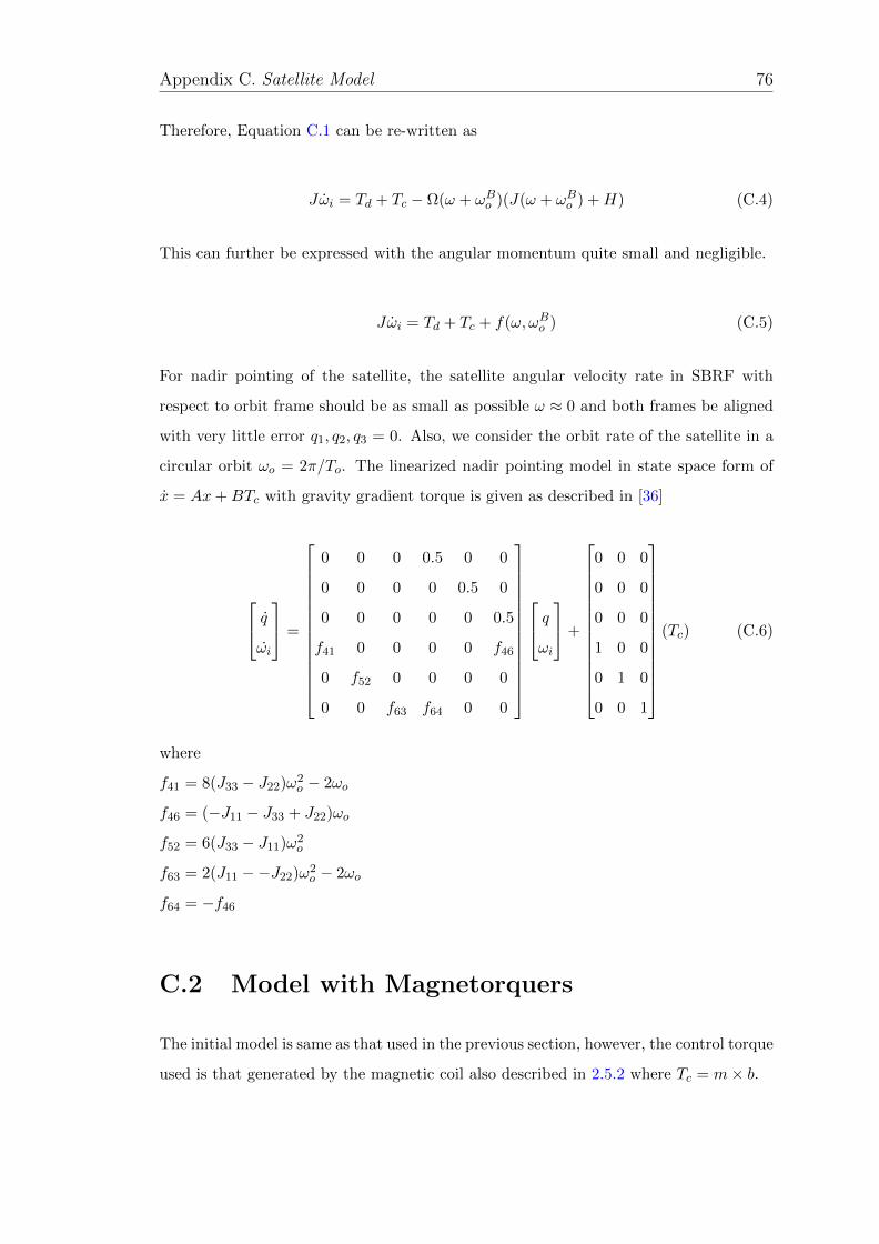
Appendix C. Satellite Model 76
Therefore, Equation C.1 can be re-written as
Jωi = Td + Tc − Ω(ω + ωBo )(J(ω + ωBo ) +H) (C.4)
This can further be expressed with the angular momentum quite small and negligible.
Jωi = Td + Tc + f(ω, ωBo ) (C.5)
For nadir pointing of the satellite, the satellite angular velocity rate in SBRF with
respect to orbit frame should be as small as possible ω ≈ 0 and both frames be aligned
with very little error q1, q2, q3 = 0. Also, we consider the orbit rate of the satellite in a
circular orbit ωo = 2π/To. The linearized nadir pointing model in state space form of
x = Ax+BTc with gravity gradient torque is given as described in [36]
qωi
=
0 0 0 0.5 0 0
0 0 0 0 0.5 0
0 0 0 0 0 0.5
f41 0 0 0 0 f46
0 f52 0 0 0 0
0 0 f63 f64 0 0
qωi
+
0 0 0
0 0 0
0 0 0
1 0 0
0 1 0
0 0 1
(Tc) (C.6)
where
f41 = 8(J33 − J22)ω2o − 2ωo
f46 = (−J11 − J33 + J22)ωo
f52 = 6(J33 − J11)ω2o
f63 = 2(J11 −−J22)ω2o − 2ωo
f64 = −f46
C.2 Model with Magnetorquers
The initial model is same as that used in the previous section, however, the control torque
used is that generated by the magnetic coil also described in 2.5.2 where Tc = m× b.

Appendix C. Satellite Model 77
The magnetic field b is also expressed based on the dipole model described in Section
3.3.1 as
b =
b1(t)
b2(t)
b3(t)
=µfa3
cosω0t sin θ
− cos θ
2 sinω0t sin θ
(C.7)
With the inclination of the spacecraft orbit and the magnetic equator θ = 0 the quater-
nion linear time invariant model is therefore reduced and given by [16]
qωi
=
0 0 0 0.5 0 0
0 0 0 0 0.5 0
0 0 0 0 0 0.5
f41 0 0 0 0 f46
0 f52 0 0 0 0
0 0 f63 f64 0 0
qωi
+
0 0 0
0 0 0
0 0 0
0 0 −b2/J11
0 0 0
−b2/J33 0 0
m1
m2
m3
(C.8)
where
f41 = 8 (J33−J22)J11
ω2o
f46 = (−J11−J33+J22)J11
ωo
f52 = 6 (J33−J11)J22
ω2o
f63 = 2 (J11−−J22)J33
ω2o
f64 = (J11+J33−J22)J33
ωo

D Abstracts Accepted for Oral Pre-
sentations
D.1 Abstract for 68th International Astronauti-
cal Congress 2017 - Tether Deployment Us-
ing High Spin Rate Control For Interplan-
etary Nanosatellite Missions
This paper presents a high spin rate control algorithm based on a Linear Quadratic
Regulator (LQR) used for tether deployment on the ESTCube-2 3U nanosatellite. The
300m long tether, consisting of 4 parallel 25µm diameter wires, will be deployed using
centrifugal force generated by spinning up the satellite. The deployed tether will be
used for a deorbiting experiment employing the plasma break technology. The attitude
control system of ESTCube-2 will use electromagnetic coils, reaction wheels and cold
gas thrusters as actuators. The LQR will be designed based on linearized satellite
dynamics. The aim of the controller is to spin up the satellite to 360 deg/s about the X-
axis (short axis) while simultaneously aligning the spin axis with the Earth’s polar axis.
The paper will also describe the design of an LQR optimal controller with controllability
and stability analysis to meet the strict pointing requirements of the ESTCube-2 Earth
observation camera and the high speed communication antenna. The simulation results
will be presented and analysed to improve controller performance. The attitude control
78

Appendix D. Conference Abstracts 79
algorithms will be flight tested on ESTCube-2 as a stepping stone for ESTCube-3 which
is planned to be launched to lunar orbit.
D.2 Abstract for 6th iCubeSat Workshop 2017 -
ESTCube-2 Nanosatellite Attitude Control
for Interplanetary Missions
This paper presents the design and study of attitude control algorithms for the ESTCube-
2/3 missions making use of electromagnetic coils, reaction wheels and cold gas thrusters
as actuators. The controllers designed are based on fulfilling the set requirements of
the ESTCube-2 mission. The 3U CubeSat is required to spin up for the centrifugal
tether deployment for the Plasma Brake experiment. The algorithm designed for this is
required to spin the satellite up to 360 deg/s about the X-axis while simultaneously en-
suring the alignment of the satellite with Earth’s polar axis. The attitude control system
is designed to also satisfy the strict pointing requirement of which a Linear Quadratic
Regulator controller (LQR) has been designed with controllability and stability analysis
based on linearized satellite dynamics and is being enhanced for tracking making use of
the reaction wheels of the satellite. In addition, we present attitude control methods to
be tested for the ESTCube-3 which is meant for the lunar orbit applying a combination
of reaction wheels and cold gas thrusters for attitude maneuvering. Results based on
simulations are therefore presented and analyzed for improved performance.
80
Non-exclusive licence to reproduce thesis and make thesis public.
I, Ikechukwu Ofodile (date of birth: 31.08.1993),
1. herewith grant the University of Tartu, Estonia a free permit (non-exclusive license)
to:
1.1. reproduce, for the purpose of preservation and making available to the public,
including for addition to the DSpace digital archives until expiry of the term of validity
of the copyright, and
1.2. make available to the public via the web environment of the University of Tartu,
including via the DSpace digital archives until expiry of the term of validity of the
copyright,
Design and Comparison of Attitude Control Modes for ESTCube-2
supervised by Dr. Andris Slavinskis and Assoc. Prof. Gholamreza Anbarjafari
2. I am aware of the fact that the author retains these rights.
3. I certify that granting the non-exclusive licence does not infringe the intellectual
property rights or rights arising from the Personal Data Protection Act.
Tartu 17.05.2017