university of vaasa faculty of technology electrical ...sgemfinalreport.fi/files/d2_3_15_part2_...
TRANSCRIPT

UNIVERSITY OF VAASA
FACULTY OF TECHNOLOGY
ELECTRICAL ENGINEERING
Elina Määttä S93545
SATE.3050 Sähkötekniikan erikoistyö
TESTING OF THE PERFORMANCE OF NOVEL ADMITTANCE CRITERION
FOR INTERMITTENT EARTH FAULT PROTECTION
Pages: 45
Submitted for evaluation: 20.5.2014
Supervisor Kimmo Kauhaniemi

1
TABLE OF CONTENTS
SYMBOLS AND ABBREVIATIONS 2
1 INTRODUCTION 3
2 INTERMITTENT EARTH FAULT 5
2.1 General 5 2.2 Fault initiation 6 2.3 Types of intermittent earth faults 7
3 PROTECTION METHODS 10 3.1 Conventional earth fault protection and related problems 10
3.2 Novel admittance criterion 11 3.3 Relay operation time settings and coordination with busbar protection 14
4 SIMULATIONS 16
4.1 Simulation model 16
4.2 Simulation parameters and constant values 19 4.3 Simulation results 20
4.3.1 Short time interval between spikes 21 4.3.2 Long time interval between spikes 30
5 CONCLUSIONS 40
REFERENCES 42
APPENDIX 44 Appendix 1. Matlab
® scripts 44

2
SYMBOLS AND ABBREVIATIONS
Symbols
f
3I0
I0Bg
I0Fd
I0
IL1, IL2, IL3
ECPS
Rf
U0
tend
tstart
Ua, Ub, Uc
Y0sum_CPS
Y0sum
Y01
Y0n
Frequency
Residual current
Zero sequence current of the background network
Zero sequence current of the protected feeder
Zero sequence current
Phase currents in phases 1,2, and 3
Cumulative phasor sum
Fault resistance
Zero sequence voltage
End time
Start time
Phase-to-earth voltages in phase a, b, and c
Cumulative phasor summing neutral admittance phasor
Fundamental frequency neutral admittance phasor
Neutral admittance phasor of the fundamental frequency
Neutral admittance phasor of the nth
harmonic frequency
Abbreviations
AC
BG
CPS
DFT
DNO
MV
Alternating Current
Background
Cumulative Phasor summing
Discrete Fourier Transform
Distribution Network Operator
Medium Voltage
OHL
PSCAD
UGC
Overhead Line
Power System Computer Aided Design, a simulation software
Underground Cabling
XLPE Cross-linked Polyethylene

3
1 INTRODUCTION
Nowadays, uninterruptable quality of electricity supply is very important. However, re-
cent storms, which have damaged medium voltage (MV) distribution networks and re-
lated long outages to customers, and new quality of supply regulations, have contributed
to build more reliable and weatherproof MV distribution networks. Therefore, distribu-
tion network operators (DNOs) have started to replace overhead lines (OHLs) by under-
ground cables also in rural areas. However, increased cabling is not a trouble-free solu-
tion. Problem with a special, very short and repetitive type of fault, an intermittent earth
fault is noticed. There have been existed intermittent earth faults in networks, but par-
ticularly recently they have risen in attention. (Mäkinen 2001:1–2; Altonen, Mäkinen,
Kauhaniemi & Persson 2003.)
During an intermittent earth fault, regular or irregular waveforms and spikes arise. Con-
ventional earth fault protection is incapable of detecting these kinds of faults. Relay may
not be able to trip the faulted feeder and situation can lead to false relay operation. In
the worst case a whole substation could be disconnected due to back-up protection,
which observes zero sequence voltage growth, i.e. neutral point displacement voltage
measured at the substation. Outages in wide area and related costs could be significant.
In normal conditions this zero sequence voltage, which is the voltage between earth and
system’s neutral point, is almost zero. (Altonen et al. 2003.) Consequently, intermittent
earth fault protection has to be implemented by other methods. Therefore, the aim of
this work was to study the performance of the novel admittance criterion for detecting
intermittent earth faults in MV distribution networks. (Wahlroos, Altonen, Uggla &
Wall 2013.)
The most important thing in intermittent earth fault protection is that the relay observes
only the fault in the faulted feeder (Arcteq 2014: 3). The novel admittance criterion for
detecting intermittent earth faults, which is based on cumulative phasor summing
(CPS), was studied more thoroughly in the simulations. The novel admittance criterion
is proven to give accurate measurement results despite the fault resistance and fault

4
type. (Wahlroos et al. 2013.) The simulation model for studying intermittent earth faults
with defined two fault scenarios was carried out by PSCAD network modelling tool.
The structure of this work consists of five chapters. After the introduction, Chapter 2
summarizes the basics of intermittent earth faults. Chapter 2 is based on my seminar
work Määttä (2014). Chapter 3 introduces the novel admittance criterion for intermittent
earth fault protection. Part of the Chapter 3 is also based on my earlier seminar work.
Chapter 4 presents the empirical part of this work, which is implemented by creating a
typical MV distribution network model by PSCAD network modelling tool with two
defined intermittent earth fault scenarios. Based on the simulation results, conclusions
are made, and which can be found in Chapter 5.

5
2 INTERMITTENT EARTH FAULT
2.1 General
An intermittent earth fault or restriking fault is special, low impedance, transient type of
earth fault, and repeated in very short time intervals, only a few milliseconds. The in-
termittent earth fault ignites and vanishes alternately. An intermittent fault is caused by
a series of cable insulation breakdowns or deterioration of insulation due to diminished
voltage withstand. Usually, insulation levels of cables, cable terminal boxes or joints are
damaged somehow as a result of cable ageing, material failure or mechanical stress situ-
ations in the long run. Also, moisture, dirt or unintentional accidents or human errors,
e.g. excavation work can lead to intermittent earth faults. At the fault place, where cable
insulation has become weaker, the phase-to-earth voltage arises and makes a spark.
Nonetheless, when current reaches its zero point for the first time, fault may experience
a self-extinguishment. (Altonen et al. 2003; Mäkinen 2001: 1–2.)
Intermittent fault is very typical fault in compensated systems consisting of under-
ground cables. Especially water treeing, which leads to intermittent earth fault situation
with XLPE-cables, is phenomenon due to, e.g. impurities in material, alternating current
(AC)-electric field and penetrating water. Moreover, rural area networks consisting both
OHLs and underground cables are relative susceptible for restriking faults. Thus, proba-
bility of earth fault density is greater due to overhead line parts. (Kumpulainen 2008;
Vamp 2009; Altonen et al. 2003.)
Fig. 1 shows a typical intermittent earth fault situation in a substation, where zero se-
quence current peaks and zero sequence voltage waveform at the faulted and healthy
feeders are illustrated. Residual current, i.e. zero sequence current, which is the sum of
three phase currents, can be measured by either each phase current via a separate current
transformer or directly by a cable current transformer, which is connected around all
three phases (Altonen et al. 2003; Mäkinen 2001: 1–2; Dlaboratory Sweden Ab. 2012.)
The amplitudes of the measured residual current spikes can be very high, several hun-

6
dred amperes. Intermittent earth fault is problematic both with healthy feeders and
faulted feeder. Relays are not able to detect fault reliably at the faulted feeder, where the
tripping should be executed. On the other hand, healthy feeders might trip falsely or
possibly the main supply might be disconnected, because zero sequence voltage stays in
high values long enough. (Wahlroos 2012.)
Figure 1. Residual currents of faulted and healthy feeders and zero sequence voltage
waveform in intermittent earth fault situation. (Wahlroos 2012.)
2.2 Fault initiation
During an intermittent earth fault, the phase-to-earth voltage reduces in the faulted
phase and the phase-to-earth voltages increase in the healthy phases. The capacitance-
to-earth of the faulted phase start to discharge i.e. produce discharge current transient
and the healthy feeder phase-to-earth capacitances start to charge, which produce charge
current transients. Charge transient frequency, f varies between 200 Hz and 1000 Hz.
Discharge transient frequency is 4–20 times bigger compared to charge transient fre-

7
quency. After succeeded extinguishment, phase-to-earth voltage of the faulted phase is
recovering and the residual voltage declines waiting for next breakdown, which can be
seen in Fig. 2. (Altonen et al. 2003.)
Figure 2. Recovery and residual voltages after an extinguishment of the fault. (Alto-
nen et al. 2003.)
2.3 Types of intermittent earth faults
Next, three different types of intermittent earth faults are presented. The examples were
recorded by a high performance fault recorder (130/20 kV) at the transformer station in
Sweden. Fig. 3 shows the first type of intermittent earth fault, where five spikes arise in
10 seconds. It is peculiar to this long fault duration between each spike, which means
that all quantities reach their zero value before next re-ignition. There is not overlapping
between spikes. Also, the zero sequence voltage reaches its zero value, and reset the
timers for zero sequence voltage relay. Therefore, malfunctions can be avoided. (Dla-
boratory Sweden Ab. 2012.)

8
Figure 3. Zero sequence voltage and sum of phase currents and close-ups in 10 sec-
onds time interval. (Dlaboratory Sweden Ab. 2012.)
The second intermittent earth fault type, which is illustrated in Fig. 4 with close-ups,
contains five spikes during less than one second. It is typical for this second intermittent
earth fault type very short time between spikes. Hence, voltage transient is reduced be-
fore the next spike, and it is overlapping. In this case, zero sequence voltage stays at the
high level, as long as the fault continues. In worst case, this type of intermittent fault
can lead to an unselective relay operation and disconnection of all feeders in the whole
substation. Zero sequence voltage does not reduce and particular time delay of the pro-
tection is reached, which leads to relay operation. In the third intermittent earth fault
type example, which is presented in Fig. 5, there exists multitude high frequency current
peaks during one second recording time. Typical for this kind of intermittent fault type
is the high frequency content in the residual current. This is because of very short dis-
tance between fault and recording place. (Dlaboratory Sweden Ab. 2012.)

9
Figure 4. Zero sequence voltage, residual current, and close-ups in 1 second time in-
terval. (Dlaboratory Sweden Ab. 2012.)
Figure 5. Zero sequence voltage and sum of phase currents and close-ups in 0.8 sec-
ond time interval. (Dlaboratory Sweden Ab. 2012.)

10
3 PROTECTION METHODS
3.1 Conventional earth fault protection and related problems
The purpose of the earth fault protection scheme is to be selective, reliable, sensitive,
and make sure that protection is valid during and after every earth fault situation. The
conventional earth fault protection is based on detecting permanent earth faults, which
follow almost fundamental frequency and sinusoidal waveforms of residual current and
zero sequence voltage. Because the behaviour of intermittent fault is rather different
compared to permanent earth fault behaviour, which can be seen in Fig. 6, detection of
it is very challenging. It has to be remembered that the precise fault mechanism of in-
termittent earth fault is not known, and some fault modes can occur in unexpected cir-
cumstances. (Kuisti et al. 1999; Lorenc, Musierowicz & Kwapisz 2003.)
Figure 6. Comparison of intermittent earth fault waveforms and permanent earth fault
waveforms. (Wahlroos et al. 2011.)
As can be seen in Fig. 6, very irregular current and voltage waveforms in case of inter-
mittent earth fault are noticed. Therefore, conventional earth fault protection relays are
incapable of detecting this kind of fault reliably and hence, more dedicated solutions for

11
detection and removing intermittent earth faults are needed. (Altonen et. al. 2003; Kuisti
et al. 1999.)
Intermittent earth faults can cause the disconnection of the substation and interrupt
power supply for a large amount of customers. This is caused by U0-back-up protection
relay tripping, because in compensated networks, where a compensation coil is connect-
ed to transformer’s neutral point either centrally or decentrally to cancel the capacitive
earth fault current almost entirely, U0 attenuates slowly between insulation breakdowns.
In compensated networks, there is also a parallel resistor connected to coil to increase
resistive earth fault current for selective relay operation. However, the parallel resistor
affects the probability of intermittent earth faults. The probability of an intermittent
earth fault is evident, when the resistance increases. Increased resistance decreases also
the magnitude of fault current. Alternatively, the higher resistance affects by the proba-
bility of intermittent earth fault by slowing the voltage rise at the faulted phase. There-
fore, the probability of the next breakdown after the previous one is decreased. (Altonen
et. al. 2003; Kuisti et al. 1999.)
3.2 Novel admittance criterion
Novel admittance based earth fault protection is a novel algorithm for earth fault protec-
tion in compensated MV distribution networks. There is combined “optimal transient
and steady-state performance into one function”. The method is based on multi-
frequency admittance measuring, where the direction of the accumulated fault phasor
points towards the fault direction. Especially, it is proven to give accurate measurement
results despite the fault resistance, and fault type. Moreover, the type of fault can be
permanent, transient or an intermittent earth fault; earth fault protection function none-
theless reliably. Because of this solution is proven to be very reliable and other protec-
tion functions for detecting, e.g. permanent earth faults, are not needed. (Wahlroos et al.
2013.)

12
The fundamental admittance frequency phasor, which ensures the sensitivity of protec-
tion, can be calculated as follows:
Y0sum = Re[Y01] + j∙Im[Y0
1 + ∑
], (3.1)
where
Y01 = 3I0
1/-U0
1 is the neutral admittance phasor of the fundamental frequency,
Y0n = 3I0
n/-U0
n is the neutral admittance phasor of the n
th harmonic frequency.
Harmonics, which are accounted for loads, transformers, compensation coils, and the
type of fault, improve the directional determination security of earth fault. Because the
harmonics are significant by earth fault protection point of view, they are utilized. Di-
rectional determination of earth fault is very simple; the protection is based on the sign
of the imaginary part of the operate quantity phasor. Operation characteristic can be
seen in Fig. 7, and it is valid for isolated and compensated networks. (Wahlroos et al.
2013.) According to Fig. 7, the left side of the operation characteristic represents the
non-operate area, and the right side of the operation characteristic represents the operate
area. The set correction angle, i.e. operation characteristic angle, separates these two
areas. The proper angle can be, e.g. 5°. (Wahlroos et al. 2013.)
Figure 7. Operation characteristic of admittance criterion. (Wahlroos et al. 2013.)

13
However, the origin of harmonics, harmonics share and amplitudes might have large
variation in time. Therefore, operation might be uncertain, and the calculation process
of threshold settings might turn out problematic. If attenuation of higher frequency
components due to fault resistance is occurred, the harmonic protection is reliable only
in case of very low-ohmic earth faults. (Wahlroos et al. 2013.)
Problems related to the traditional fundamental frequency, transients, and harmonic-
based methods for earth fault protection can be avoided by using Cumulative Phasor
Summing (CPS). It is a method, which utilizes discrete Fourier transform (DFT) calcu-
lation, but is still accurate in case of measured signals are temporary, distorted or are
containing other frequency components than fundamental or have non-periodic compo-
nents. CPS is a simple method, which is easy to implement and realize. (Wahlroos et al.
2013.)
The cumulative phasor schema is presented in Fig. 8. Into the result, values of measured
complex DFT phasors in phasor format from start time to end time are added. Cumula-
tive phasor sum can be calculated according to equation (Wahlroos et al. 2013.)
ECPS = ∑ end tstart
= ∑ e[ end tstart
+ j∙∑ Im[ end tstart
, (3.2)
where
Re[E(i)] = real part of phasor E, and
Im[E(i)] = imaginary part of phasor E.

14
Figure 8. CPS concept. (Wahlroos et al. 2013.)
ECPS phasor can be, e.g. current, power, impedance or admittance phasor. The sufficient
time interval between the phasor accumulation considering fault transients can be, e.g.
2.5 ms. And, when admittance measurement is used, CPS can be defined as follows:
Y0sum_CPS = ∑ e[
end
start +j∙∑ Im[
end
start + ∑
, (3.3)
This technique is very valid and reliable, because the accumulated phasor is pointing
towards the fault direction. CPS method also produces a sufficient amplitude estimation
of the operation quantity. This solution is valid in case of transient and intermittent
faults, when high distortions of residual quantity, non-fundamental frequencies or non-
periodic components are occurred. The method is already used in ABB REF615 IEDs,
where the first version of the algorithm is utilized. (Wahlroos et al 2013.)
3.3 Relay operation time settings and coordination with busbar protection
It is clear that in pursuance of setting the intermittent earth fault protection, zero se-
quence voltage protection of the busbar has to be coordinated in the right way. The
faulted feeder should be always disconnected before the operation of the busbar protec-

15
tion with sufficient margin. However, intermittent earth faults can cause stress for net-
work, and therefore the operation of the protection should be done relative fast. It is
recommended that the proper reset time of an intermittent earth fault stage would be
500 ms, calculated from the first occurred spike. The value should not be lower than
450 ms. In this case the operation requires at least two spikes to be noticed, which is a
typical situation in compensated networks, because in these networks spikes occur less
frequently. If the busbar protection is set to very fast, under 1 s, it should be revised.
The back-up protection should not be faster than intermittent earth fault operation time
with added circuit operate time and reset time of the zero sequence voltage protection.
(Arcteq 2014: 4–5.)

16
4 SIMULATIONS
Intermittent earth fault protection was studied by novel admittance criterion based on
CPS. The intermittent earth fault model was based on the calculation of the accumulated
phasor sum of DFTs at fundamental frequency. In this work, the purpose was to simu-
late the performance of the admittance criterion in case of intermittent earth faults in
two different situations. And also to find out how well the novel admittance criterion
can detect intermittent earth faults in compensated cabled MV distribution network,
when the time between spikes was short and long. In the first simulated situation in this
work, the time between spikes was shorter (50 ms) compared to the second case, where
the time between spikes was considerably longer (500 ms).
The simulations were created by PSCAD network modelling tool. The network model,
which was used, was created by Jaakkola (2012). The model was modified partly to
achieve the desired intermittent earth fault scenarios. The intermittent earth fault control
segment was added to model to simulate intermittent earth faults in network. The inter-
mittent earth fault model was created originally by Olavi Mäkinen, and it was also used
in his Licentiate thesis: Mäkinen (2001). The simulation results in case of defined fault
scenarios were created by a multi-run block and saved to separate files. The results were
transferred into Excel for essential calculations. Finally, the results were transferred into
Matlab®, where the protection graphs were created. In the next sections, the main parts
of the simulation model and the performance of the protection in each case using novel
admittance criterion for detecting intermittent earth faults are introduced.
4.1 Simulation model
Because intermittent earth faults occur mostly in compensated cabled networks, the pro-
tected feeder was totally cabled. The network model consisted of 110 kV main supply,
110/20 kV main transformer, parallel resistor, which was adjusted to produce 5 A resis-
tive current, centralized compensation coil, and a busbar, which consisted of four feed-
ers (2 OHLs and 2 cables) and their load, according to Fig. 9. The load in the back-

17
ground (BG) network was 8 MW and in the protected feeder, 2 MW or 2 MW per feed-
er.
Figure 9. Main supply, 110/20 kV main transformer, protected feeder, BG network
and the load of the BG network.
The central coil compensated 10 km from the beginning of each feeder, and the decen-
tralized coils compensated the rest of the feeders. The cable feeders were decentrally
compensated in every 5 km, and only one compensation coil compensated each OHL
feeder. The coils at the OHL feeders located in the middle of the OHL feeders.
Figure 10 shows the protected feeder and its load with decentrally installed compensa-
tion coils. Loads were continuously connected, and the resistances of loads were delta-
connected. The healthy state U0 was adjusted to be 2 % of the main voltage, which was
created by star-connected resistances referrering to shunt conductances. 2 % was an es-
timation of the typical asymmetry of a real network. The cable type AHXAMK-W

18
3∙ 85+35, and the OHL type aven 54/9 were used. The feeder sections were created
by pi-sections. The length of each trunk line pi-section was 5 km, and branch line
2.5 km. The total length of the network was 220 km.
Figure 10. Protected feeder and its load, decentrally installed compensation coils, and
intermittent earth fault section.
Intermittent earth fault phenomenon to network model was created, which can be seen
in Fig. 10 below the protected feeder. Figure 11 shows the control segment for intermit-
tent earth fault. It was possible to adjust ON and OFF delays of the intermittent earth
fault, fault resistance, insulation level, intermittent earth fault start time, and fault dura-
tion time. In both cases the fault duration time was 1 s, and the fault start time was set to
0.2 s. For the protection method based on the cumulative phasor sum of the admittances
from the protected feeder and BG network, multi-run block saved the instantaneous re-
sults at every 2.5 ms (Wahlroos et al 2013). The samples were taken during 1 s, i.e. be-
tween 0.2 s and 1.2 s. Some variation to the intermittent earth fault signal was created

19
by a random number generator, which modified the set insulation level. The random
number generator produced a new number, whenever the input timer signal changed.
However, the probability was adjusted to 1 %, which meant that the number was varied
only between 99 % and 100 %. It can be concluded that the variation of produced num-
ber was negligible. When the set insulation level was reached, the fault was switched
on. And after the set time delay, which was set to 20 ms, the fault was allowed to switch
off at the next zero crossing of the fault current.
Figure 11. The control segment for intermittent earth fault.
4.2 Simulation parameters and constant values
In this model, the cable and OHL parameters were constant and can be found in Table 1.
It was possible to adjust different factors, but only fault location, insulation level, and
OFF delay were varied. The fault locations were at the beginning and at the end of the
protected feeder, and also in the BG network. Compensation degree was kept at 0.95.
Ivika
TIME
Ulimit
Ulimit
Tf
Tf
*-1
*
Utaso
NEG. DIELECTRIC INSULATION LEVEL
Läpilyö...
jännitt...
laskenta
D+
F
+
Uvika_abs
Tka
tk
Vain
käynnistys-
hetken asetus
| X |Uvvika
1
Raja
A
B Compar-ator
POS. DIELECTRIC INSULATION LEVEL
Maasulku...
vaiheessa A
A
B
Ctrl
Ctrl = 1
Fault current
Vian
kestoaika
DURATION
TIME
INS. LEVEL
Eristys-
tason
asetus
RMSIFault_rms
CPanel
IFault_rms
Random
30 1
7.74
1.01
CPanel
20
0
INS. LEVEL
15
kV
INITIATE
0
TYPE
0
INT NORM10
0.1
KATKaloitus
0.2se
c
10
0.1
TIME
0.2
se
c2
0.001
DURATION
2
se
c
Td
D+
F
+
After the delay, current reaches zero
In this model, the delay was set to 20 ms
Delay
1
MaasulkuS Q
QR C
1
TIME 1
A
B
Ctrl
Ctrl = 00
20
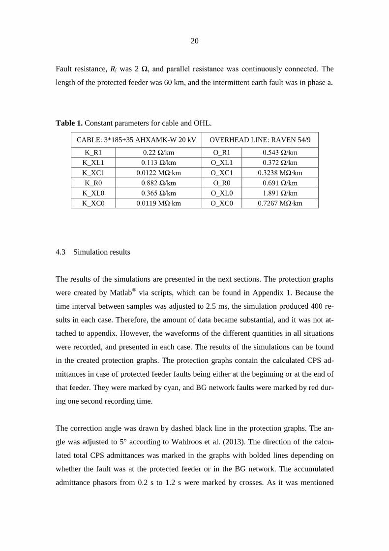
Fault resistance, Rf was 2 Ω, and parallel resistance was continuously connected. The
length of the protected feeder was 60 km, and the intermittent earth fault was in phase a.
Table 1. Constant parameters for cable and OHL.
CABLE: 3*185+35 AHXAMK-W 20 kV OVERHEAD LINE: RAVEN 54/9
K_R1 . Ω/km O_R1 .543 Ω/km
K_XL1 . 3 Ω/km O_XL1 .37 Ω/km
K_XC1 . MΩ∙km O_XC1 .3 38 MΩ∙km
K_R0 .88 Ω/km O_R0 0.691 Ω/km
K_XL0 .365 Ω/km O_XL0 .89 Ω/km
K_XC0 0.0119 MΩ∙km O_XC0 0.7267 MΩ∙km
4.3 Simulation results
The results of the simulations are presented in the next sections. The protection graphs
were created by Matlab® via scripts, which can be found in Appendix 1. Because the
time interval between samples was adjusted to 2.5 ms, the simulation produced 400 re-
sults in each case. Therefore, the amount of data became substantial, and it was not at-
tached to appendix. However, the waveforms of the different quantities in all situations
were recorded, and presented in each case. The results of the simulations can be found
in the created protection graphs. The protection graphs contain the calculated CPS ad-
mittances in case of protected feeder faults being either at the beginning or at the end of
that feeder. They were marked by cyan, and BG network faults were marked by red dur-
ing one second recording time.
The correction angle was drawn by dashed black line in the protection graphs. The an-
gle was adjusted to 5° according to Wahlroos et al. (2013). The direction of the calcu-
lated total CPS admittances was marked in the graphs with bolded lines depending on
whether the fault was at the protected feeder or in the BG network. The accumulated
admittance phasors from 0.2 s to 1.2 s were marked by crosses. As it was mentioned

21
earlier about the operation time of the relay, the adequate time could be 0.5 ms calculat-
ing from the first spike. In these simulations the first spike occurred at 0.2 s. Conse-
quently, relay should operate at 0.7 ms. Therefore, the accumulated admittance phasor
at 0.7 s was marked by black crosses in the graphs. This showed where the accumulated
admittance phasor was located at that time.
4.3.1 Short time interval between spikes
In this case the insulation level was 10 kV, Rf was 2 Ω, ON delay was 20 ms, and OFF
delay was 50 ms. The time between spikes was adjusted to be short, 50 ms.
Intermittent earth fault at the beginning of the protected feeder
Fig. 12 shows the typical waveforms of the phase-to-earth voltages Ua, Ub, Uc, zero se-
quence voltage U0, zero sequence currents of the protected feeder I0Fd, and healthy feed-
ers I0Bg measured at the substation, when the fault located at the beginning of the pro-
tected feeder. In this case the time between spikes was adjusted to be relative short
(50 ms), which can be seen in Fig. 12. Phase-to-earth voltage Ua in the faulted phase a,
reduced, and recovered between the short spikes due to fault. Respectively, healthy
phase-to-earth voltages increased during the fault. Zero sequence current at the protect-
ed feeder contained relative high current peaks. In this case, zero sequence voltage be-
haved almost in the same way as in case of permanent earth fault situation. This means
that, when spikes occur often enough, earth fault protection can detect the intermittent
earth faults easier, and the operation of the back-up protection can be avoided.

22
Figure 12. Waveforms of the Ua, Ub, Uc, U0, I0Fd and I0Bg in case of fault located at the
beginning of the protected feeder with short time interval between spikes.
Figure 13 shows the instantaneous admittances of the protected feeder and the BG net-
work, and Fig. 14 the performance of the novel admittance criterion using CPS in case
of intermittent earth fault at the beginning of the protected feeder. The left side in the
graphs represented the non-operate area and the right side represented the operate area.
The total CPS admittance of the BG network pointed to the non-operate area, even
though the most of the instantaneous admittances were located very near the boundary
line. Instantaneous admittances at the protected feeder were located more clearly in the
operating area. Calculated total CPS admittance of the protected feeder was clearly
pointing towards operating area, which meant that protection operated correctly in this
case, and there was a sufficient margin to boundary line. It referred that protection with
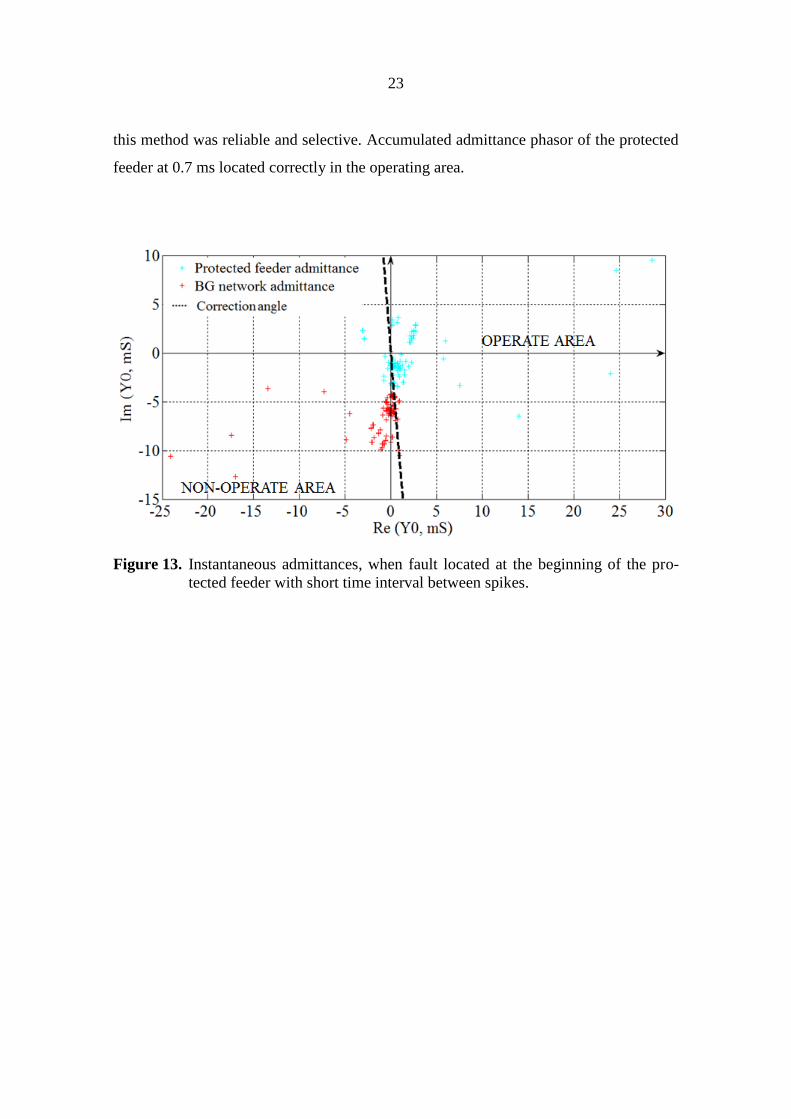
23
this method was reliable and selective. Accumulated admittance phasor of the protected
feeder at 0.7 ms located correctly in the operating area.
Figure 13. Instantaneous admittances, when fault located at the beginning of the pro-
tected feeder with short time interval between spikes.

24
Figure 14. Calculated CPS admittances in case of intermittent earth fault at the begin-
ning of the protected feeder with short time interval between spikes.
Intermittent earth fault at the end of the protected feeder
Fig. 15 shows the typical waveforms in this case. It can be seen in Fig. 15 that the wave-
forms did not change much compared to situation above, see Fig. 12. However, in the
faulted phase according to Fig. 15, it can be seen that the voltage between spikes varied
more compared to situation in Fig. 12.

25
Figure 15. Waveforms of the Ua, Ub, Uc, U0, I0Fd and I0Bg in case of fault located at the
end of the protected feeder with short time interval between spikes.
Fig 16 shows the instantaneous admittances and Fig. 17 the performance of the novel
admittance criterion using CPS in this case. The total CPS admittance of the BG net-
work was pointing correctly to the non-operating area. Most of the instantaneous admit-
tances at the protected feeder located correctly in the operating area. When calculating
the total CPS admittance of the protected feeder, it was pointing towards the operating
area. Accumulated admittance phasor at 0.7 ms guaranteed the correct functioning of
the protection.

26
Figure 16. Instantaneous admittances, when fault located at the end of the protected
feeder with short time interval between spikes.

27
Figure 17. Calculated CPS admittances in case of intermittent earth fault at the end of
the protected feeder with short time interval between spikes.
Intermittent earth fault in the BG network
Fig. 18 shows the waveforms of phase-to-earth voltages, zero sequence currents of the
protected feeder and the BG network, and zero sequence voltage. It can be seen that the
waveforms did not change much compared to situations, where fault was located at the
beginning and at the end of the protected feeder.

28
Figure 18. Waveforms of the Ua, Ub, Uc, U0, I0Fd and I0Bg in case of fault located in the
BG network with short time interval between spikes.
Fig. 19 shows the instantaneous admittances and Fig. 20 the accumulated admittance
phasors during the fault. In case of intermittent earth fault located in the BG network,
the most instantaneous admittances measured from the BG network located now in the
operating area according to Fig. 19. The direction of all CPS admittances of the BG
network located also in the operating area, including the accumulated admittance phasor
at 0.7 s. Respectively, the accumulated admittance phasors of the protected feeder were
pointing towards the non-operate area. Consequently, protection was selective also in
this case despite the fault located in the BG network.

29
Figure 19. Instantaneous admittances, when fault located in the BG network with short
time interval between spikes.
Figure 20. Calculated CPS admittances in case of intermittent earth fault in the BG
network with short time interval between spikes.

30
4.3.2 Long time interval between spikes
Because the simulated network was large, the proper time interval between spikes was
adjusted to be 500 ms in the second case. Therefore, the next simulations were created
by using this time interval, where the spikes occurred less frequently. The insulation
level in this case was 15 kV, Rf was 2 Ω, ON delay was 20 ms, and OFF delay was
500 ms, which was now longer compared to the previous simulation case.
Intermittent earth fault at the beginning of the protected feeder
In the second simulation case, the waveforms of phase-to-earth voltages, zero sequence
currents of the protected feeder and the BG network, and zero sequence voltage can be
found in Fig. 21. The waveforms of zero sequence voltage and zero sequence current to
test simulation case according to Arcteq (2014: 18) were compared. Network was in
close to resonance point, and fault was located 3 km from the substation. The network,
which was simulated according to Arcteq (2014: 18.), was large (~100 A). On the other
hand, the created network model in this work produced apprx. 400 A. Simulated zero
sequence voltage and current waveforms examples can be found in Fig. 22. It can be
seen that the waveforms correspond quite a lot to simulation case according to Figs. 21
and 22, even though the created network was larger, and compensation degree and fault
locations were a bit different.
During the simulation time according to Fig. 21, there existed two spikes. Voltage at the
faulted phase recovered, and the voltages at the healthy feeders increased, when fault
occurred, but started to decrease after that. Zero sequence voltage decreased after the
fault appeared, but it started to increase again, when the second spike occurred. Zero
sequence voltage did not have time to reach zero before the next spike. Two high spikes
in zero sequence currents were noticed.

31
Figure 21. Waveforms of the Ua, Ub, Uc, U0, I0Fd and I0Bg in case of long time interval
between spikes, and fault located at the beginning of the protected feeder.
Figure 22. U0 and I0 waveforms of the example simulation case, where the large net-
work was close to resonance point, and fault located 3 km from substation.
(Arcteq 2014: 18.)

32
Fig. 23 shows the instantaneous admittances and Fig. 24 the accumulated admittance
phasors of the protected feeder and BG network in case of fault located at the beginning
of the protected feeder. When the time between spikes was now longer, the most instan-
taneous admittances of the BG network located very near the boundary line according to
Fig. 23. However, the calculated total CPS admittance in this case located correctly in
the non-operating area. The total accumulated admittance phasor of the protected feeder
located very near the boundary line, but in the operating area. The accumulated admit-
tance phasor of the protected feeder at 0.7 ms, was also located in the right area. It
meant that the relay operation would operate correctly at that time. However, the margin
to the boundary line was clearly smaller compared to situation, when the time between
spikes was shorter. In this case, the probability of errors could impact on the operation
of the protection. Moreover, the correction angle was in all situations adjusted to 5°. If it
had been e.g. in this case 10°, malfunctions of protection would have probably occurred.
Therefore, the set correction angle (5°) was accurate.
Figure 23. Instantaneous admittances, when fault located at the beginning of the pro-
tected feeder with long time interval between spikes.

33
Figure 24. Calculated CPS admittances in case of intermittent earth fault at the begin-
ning of the protected feeder with long time interval between spikes.
Intermittent earth fault at the end of the protected feeder
When fault located at the end of the protected feeder, the waveforms recorded in this
case can be found in Fig. 25. The waveforms seem to be relative similar also in this case
compared to situation introduced in Figs. 21 and 22.

34
Figure 25. Waveforms of the Ua, Ub, Uc, U0, I0Fd and I0Bg in case of long time interval
between spikes, and fault located at the end of the protected feeder.
Fig. 26 shows the instantaneous admittances and Fig. 27 the accumulated admittance
phasors measured from the BG network and protected feeder in case of long time inter-
val between spikes, and fault located at the end of the protected feeder. The perfor-
mance of the protection did not change considerably compared to situation above ac-
cording to Fig. 27. The total CPS admittance of the protected feeder located in the same
way in the operating area, and the total CPS admittance of the BG network located in
the non-operating area. In this case, the margin to the boundary line was also small. If
the applied relay operation time was used, the protection would have operated correctly.

35
Figure 26. Instantaneous admittances, when fault located at the end of the protected
feeder in case of long time interval between spikes.

36
Figure 27. Calculated CPS admittances in case of intermittent earth fault at the end of
the protected feeder with long time interval between spikes.
Intermittent earth fault in the BG network
In case of intermittent earth fault located in the BG network, the recorded waveforms in
this case can be found in Fig. 28. Also in this case, the waveforms seemed to behave in
the same way, as in the previous cases, where the fault located at the beginning and at
the end of the protected feeder.

37
Figure 28. Waveforms of the Ua, Ub, Uc, U0, I0Fd and I0Bg in case of long time interval
between spikes, and fault located in the BG network.
Fig. 29 shows the instantaneous admittances and Fig. 30 the accumulated admittance
phasors during fault in case of fault located in the BG network. The total CPS admit-
tance and the accumulated admittance phasor at 0.7 s of the BG network located cor-
rectly now in the operating area, but the distance to set boundary line was very small.
This was accounted for the instantaneous admittances, most of which located very near
the boundary line and the non-operate area. In this case, errors of protection quantities
should be considered carefully. The total CPS admittance of the protected feeder located
in the non-operate area. Consequently, even though both CPS admittances located near
the boundary line, protection should operate correctly. In this case the effect of possible
errors in protection quantity measurements should be also considered.

38
Figure 29. Instantaneous admittances, when fault located in the BG network in case of
long time interval between spikes.

39
Figure 30. Calculated CPS admittances in case of intermittent earth fault in the BG
network with long time interval between spikes.

40
5 CONCLUSIONS
The aim of this work was to study the performance of the novel admittance criterion for
detecting intermittent earth faults in MV distribution networks. Intermittent fault is a
special type of fault, which is caused by series cable insulation breakdowns or deteriora-
tion due to diminished voltage withstand. There have been existed intermittent earth
faults in networks, but particularly recently they have risen in attention. This is because
of increased UGC and more demanded uninterruptable power supply. A problem with
intermittent earth faults is that traditional earth fault protection is incapable of detecting
such irregular and non-periodic waveforms. Therefore, earth fault protection against in-
termittent earth faults is rather challenging. In the worst case, the whole substation
might be interrupted. This would cause naturally long outages for customers and con-
siderable costs for DNOs. Consequently, earth fault protection from intermittent faults
in MV distribution networks has become very important, because it seems the general
trend is going towards increased UGC. Also in future, natural ageing of the existing ca-
bles will probably increase the amount of intermittent earth faults.
At the moment there exist few methods to protect MV distribution network from inter-
mittent earth faults. One of these methods is novel admittance criterion, which is based
on cumulative phasor summing (CPS). This method was studied more thoroughly in this
work. This novel criterion was studied in two different cases via PSCAD simulations.
The novel admittance criterion facilitates the protection considerably, because the ac-
cumulated admittance phasor points the fault direction clearly. Admittance criterion is
proven to give accurate measurement results despite the fault resistance and fault type.
Therefore, other protection functions for detecting, e.g. permanent earth faults, are not
needed, and intermittent earth faults can be detected reliably. However, relay operation
time settings should be done carefully, and make sure that the coordination with busbar
protection, i.e. zero sequence voltage setting, is done in the right way.
According to simulations in this work, the novel admittance criterion based on CPS de-
tected the intermittent earth faults in both cases. When the time interval between spikes
was shorter (50 ms), the admittance criterion was more reliable, because there existed

41
more margin to set boundary line. On the other hand, when the time between spikes was
longer (500 ms), the protection was capable of detecting the faults correctly, but now
the accumulated admittance phasors were located more near the boundary line. In this
case, the possible errors, which were not analysed in this work, should be also consid-
ered. The set correction angle seems to be accurate according to simulations. For exam-
ple, if it was set to 10°, the problems would have probably occured in case of long time
interval between spikes. It is also important to set accurate relay operation time. In these
simulations, it was assumed to be 0.5 s, which meant that relay should operate at 0.7 s
from the start of the simulation. The value seem to be accurate according to simulations
in both cases, but especially when the network is large, spikes arise less frequently.
Thus, the coordination with the busbar protection should be done in the right way. It is
recommended that the proper time should not be lower than 1 s.
Consequently, the simulations of this work proved that the novel admittance criterion is
very promising method for detecting intermittent earth faults in case of defined time in-
tervals between faults. However, the protection quantity calculations in the created
model were based on fundamental frequency signals. Therefore, the results may not be
as accurate as possible, because multi-frequency signals were not considered. In future,
these should be also considered and studied. In this work, only two different intermittent
earth fault cases were studied. Moreover, intermittent earth faults and this novel admit-
tance criterion are studied still fairly little. More field tests and simulations in different
network topologies in order to be completely sure that this method operates correctly
are needed. For example, in this work, the protected feeder was totally cabled, but in-
termittent earth faults occur also in networks, which consist of OHL feeders. Moreover,
variations of different compensation degrees and fault resistances should be studied.
When earth fault protection is reliable also in case of intermittent earth faults in MV dis-
tribution networks, longer operating life for network equipment and underground cables
will be achieved, and unnecessary supply interruptions can be avoided.

42
REFERENCES
Altonen, J., Mäkinen, O., Kauhaniemi, K., Persson, K. (2003). Intermittent earth faults -
need to improve the existing feeder earth fault protection schemes? CIRED 17th
In-
ternational Conference on Electricity Distribution, 3:48, 1–6. Barcelona, Spain
Arcteq (2014). Protection settings and secondary testing of intermittent earth fault func-
tion. Application note. 26 p. [online] [cited 12 May 2014] Available at: <URL:
http://www.arcteq.fi/products/product-by-application/intermittent-earth-fault-
protection>.
Dlaboratory Sweden Ab. (2012). A method for detecting earth faults. (Akke, M.) WO
Pat. Appl. 2012/171694 A1, publ. 20.12.2012. 55 p.
Jaakkola, J. (2012). Earth fault in compensated rural network. WP 2.3.12 Large scale
cabling. University of Vaasa. SGEM PSCAD Model Library. Unpublished. 27 p.
Kuisti, H., Altonen, J., Svensson, H., Isaksson, M. (1999). Intermittent earth faults chal-
lenge conventional protection schemes. International Conference on Electricity Dis-
tribution, 3:3. Nice, France.
Kumpulainen, L. (2008). A cost effective solution to intermittent transient earth fault
protection. Vamp/Vaasa Electronics Group. Presentation. Unpublished [cited Febru-
ary 27, 2014].
Lorenc, J., Musierowicz, K., Kwapisz, A. (2003). Detection of the intermittent earth
faults in compensated MV network. IEEE Conference on Power Tech Proceedings,
2,6. Bologna, Italy.
Mäkinen, O. (2001). Keskijänniteverkon katkeileva maasulku ja relesuojaus. (Intermit-
tent earth fault and relay protection in medium voltage network.) In Finnish. Licen-
tiate thesis. Tampere University of Technology. Tampere. 107 p.

43
Määttä, E. (2014). Intermittent earth fault protection. Seminar work. Faculty of Tech-
nology. University of Vaasa. Vaasa. 23 p.
Sauna-Aho, S. (2013). Intermittent transient earth faults. Vamp. Presentation. Un-
published. [cited March 11, 2014].
Vamp (2009). Intermittent transient earth fault protection. Application note. [online].
[cited March 11, 2014] Available at: URL: http://www-fi.vamp.fi/Technical%20
papers/Application%20notes/English/AN200.EN003%20Intermittent%20transient%
20 earth%20fault%20protection.pdf>.
Wahlroos, A., Altonen, J., Hakola, T., Kemppainen T. (2011). Practical application and
performance of novel admittance based earth fault protection in compensated MV
networks. CIRED 21st Internationl Conference on Electricity Distribution, 0793, 1–
4. Frankfurt, Germany.
Wahlroos, A., Altonen, J., Uggla, U., Wall, D. (2013). Application of novel cumulative
phasor sum measurement for earth fault protection in compensated MV networks.
CIRED 22nd
International Conference on Electricity Distribution, 607:1–4. Stock-
holm, Sweden.
Wahlroos, A. (2012). Admittanssimittaukseen pohjautuva maasulkusuojaus. (Earth fault
protection of admittance-based measuring). In Finnish. Presentation. ABB Oy. Dis-
tribution Automation, Finland. Unpublished.

44
APPENDIX
Appendix 1. Matlab®
scripts
Instantaneous admittances
I=A(:,1);
ang=A(:,2);
plot(I,ang,'c+');
hold on;
I=A(:,3);
ang=A(:,4);
plot(I,ang,'r+');
hold on;
lineLength = 30;
angle = (-85);
x(1) = cosd (-85);
y(1) = sind (-85);
x(2) = x(1) + lineLength * cosd(angle);
y(2) = y(1) + lineLength * sind(angle);
plot(x, y, 'k');
hold on;
lineLength = 30;
angle = (95);
x(1) = cosd (95);
y(1) = sind (95);
x(2) = -x(1)+ lineLength * cosd(angle);
y(2) = y(1) + lineLength * sind(angle);
plot(x, y, 'k');
hold on;
axis equal;
grid on;
CPS admittances
I=A(:,1); ang=A(:,2); plot(I,ang,'c+'); hold on;
I=A(:,3); ang=A(:,4); plot(I,ang,'r+'); hold on;
I=A(:,5);

45
ang=A(:,6); plot(I,ang,'c-'); hold on;
I=A(:,7); ang=A(:,8); plot(I,ang,'r-'); hold on;
I=A(:,9); ang=A(:,10); plot(I,ang,'k+'); hold on;
I=A(:,11); ang=A(:,12); plot(I,ang,'k+'); hold on;
lineLength = 30; angle = (-85); x(1) = cosd (-85); y(1) = sind (-85); x(2) = x(1) + lineLength * cosd(angle); y(2) = y(1) + lineLength * sind(angle); plot(x, y, 'k'); hold on;
lineLength = 30; angle = (95); x(1) = cosd (95); y(1) = sind (95); x(2) = -x(1)+ lineLength * cosd(angle); y(2) = y(1) + lineLength * sind(angle); plot(x, y, 'k');
axis equal; hold on;
grid on;