university of warwick institutional repository: in international finance bygino cenedese a thesis...
TRANSCRIPT

University of Warwick institutional repository: http://go.warwick.ac.uk/wrap
A Thesis Submitted for the Degree of PhD at the University of Warwick
http://go.warwick.ac.uk/wrap/49399
This thesis is made available online and is protected by original copyright.
Please scroll down to view the document itself.
Please refer to the repository record for this item for information to help you to cite it. Our policy information is available from the repository home page.

Essays in International Finance
by Gino Cenedese
A thesis submitted in partial fulfilment
of the requirements for the degree of
Doctor of Philosophy in Finance
Warwick Business School
The University of Warwick
September 2011
Contents
Overview 1
1 Average variance, average correlation and currency returns 13
1.1 Introduction . . . . . . . . . . . . . . . . . . . . . . . . . . . . . . . . . . 13
1.2 Measures of Return and Risk for the Carry Trade . . . . . . . . . . . . . 18
1.2.1 FX Data . . . . . . . . . . . . . . . . . . . . . . . . . . . . . . . . 18
1.2.2 The Carry Trade for Individual Currencies . . . . . . . . . . . . . 19
1.2.3 The Carry Trade for a Portfolio of Currencies . . . . . . . . . . . 20
1.2.4 FX Market Variance . . . . . . . . . . . . . . . . . . . . . . . . . 21
1.2.5 Average Variance and Average Correlation . . . . . . . . . . . . . 22
1.2.6 Systematic and Idiosyncratic Risk . . . . . . . . . . . . . . . . . . 23
1.3 Predictive Regressions . . . . . . . . . . . . . . . . . . . . . . . . . . . . 25
1.4 Empirical Results . . . . . . . . . . . . . . . . . . . . . . . . . . . . . . . 28
1.4.1 Descriptive Statistics . . . . . . . . . . . . . . . . . . . . . . . . . 28
1.4.2 The Decomposition of Market Variance . . . . . . . . . . . . . . . 29
1.4.3 Predictive Regressions . . . . . . . . . . . . . . . . . . . . . . . . 29
1.5 Robustness and Further Analysis . . . . . . . . . . . . . . . . . . . . . . 32
1.5.1 The Components of the Carry Trade . . . . . . . . . . . . . . . . 32
1.5.2 Additional Predictive Variables . . . . . . . . . . . . . . . . . . . 32
1.5.3 The Numeraire Effect . . . . . . . . . . . . . . . . . . . . . . . . . 33
1.5.4 VIX, VXY and Carry Trade Returns . . . . . . . . . . . . . . . . 34
1.5.5 Conditional Skewness . . . . . . . . . . . . . . . . . . . . . . . . . 36
i

Contents
1.6 Augmented Carry Trade Strategies . . . . . . . . . . . . . . . . . . . . . 37
1.6.1 The Strategies . . . . . . . . . . . . . . . . . . . . . . . . . . . . . 37
1.6.2 No Transaction Costs . . . . . . . . . . . . . . . . . . . . . . . . . 38
1.6.3 The Effect of Transaction Costs . . . . . . . . . . . . . . . . . . . 39
1.7 Conclusion . . . . . . . . . . . . . . . . . . . . . . . . . . . . . . . . . . . 41
1.A Notes on the bootstrap procedure . . . . . . . . . . . . . . . . . . . . . . 42
1.A.1 Bootstrap Standard Errors . . . . . . . . . . . . . . . . . . . . . . 42
1.A.2 Bootstrap Hypothesis Testing . . . . . . . . . . . . . . . . . . . . 43
2 On the evolution of the exchange rate response to fundamental shocks 65
2.1 Introduction . . . . . . . . . . . . . . . . . . . . . . . . . . . . . . . . . . 65
2.2 Foreign Exchange Excess Returns . . . . . . . . . . . . . . . . . . . . . . 68
2.3 Empirical Approach . . . . . . . . . . . . . . . . . . . . . . . . . . . . . . 70
2.3.1 Model . . . . . . . . . . . . . . . . . . . . . . . . . . . . . . . . . 70
2.3.2 Estimation . . . . . . . . . . . . . . . . . . . . . . . . . . . . . . . 73
2.4 Data and Stability Tests . . . . . . . . . . . . . . . . . . . . . . . . . . . 74
2.5 Empirical Results . . . . . . . . . . . . . . . . . . . . . . . . . . . . . . . 76
2.5.1 Volatilities . . . . . . . . . . . . . . . . . . . . . . . . . . . . . . . 76
2.5.2 Impulse Responses . . . . . . . . . . . . . . . . . . . . . . . . . . 77
2.6 Conclusion . . . . . . . . . . . . . . . . . . . . . . . . . . . . . . . . . . . 82
2.A Priors . . . . . . . . . . . . . . . . . . . . . . . . . . . . . . . . . . . . . 84
2.B Posteriors . . . . . . . . . . . . . . . . . . . . . . . . . . . . . . . . . . . 85
3 Currency fair value models 109
3.1 Introduction . . . . . . . . . . . . . . . . . . . . . . . . . . . . . . . . . . 109
3.2 Currency Fair Value in the Historical Context . . . . . . . . . . . . . . . 112
3.3 Characteristics of Fair Value Models . . . . . . . . . . . . . . . . . . . . 116
3.3.1 Horizon/Frequency . . . . . . . . . . . . . . . . . . . . . . . . . . 116
3.3.2 Direct econometric estimation versus “methods of calculation” . . 118
3.3.3 Treatment of External Imbalances . . . . . . . . . . . . . . . . . 119
ii
Contents
3.3.4 Real versus Nominal Exchange Rates . . . . . . . . . . . . . . . . 121
3.3.5 Bilateral versus Effective Exchange Rate . . . . . . . . . . . . . . 121
3.3.6 Time Series versus Cross-Section or Panel . . . . . . . . . . . . . 122
3.3.7 Model Maintenance . . . . . . . . . . . . . . . . . . . . . . . . . . 123
3.4 Models/Taxonomy . . . . . . . . . . . . . . . . . . . . . . . . . . . . . . 124
3.4.1 “Adjusted PPP”: Harrod-Balassa-Samuelson and Penn Effects . . 124
3.4.2 The Underlying Balance approach . . . . . . . . . . . . . . . . . . 125
3.4.3 The Behavioural Equilibrium Exchange Rate Family of Models . . 128
3.4.4 The natural real exchange rate (NATREX) . . . . . . . . . . . . . 131
3.4.5 The Indirect Fair Value . . . . . . . . . . . . . . . . . . . . . . . . 132
3.5 IMF CGER - Consultative Group on Exchange Rate Issues . . . . . . . . 135
3.5.1 The Macroeconomic Balance (MB) Approach . . . . . . . . . . . 137
3.5.2 The Equilibrium Real Exchange Rate (ERER) Approach . . . . . 139
3.5.3 The External Sustainability (ES) Approach . . . . . . . . . . . . 141
3.5.4 The Importance of Trade Elasticities . . . . . . . . . . . . . . . . 142
3.6 Goldman Sachs GSDEER . . . . . . . . . . . . . . . . . . . . . . . . . . 144
3.6.1 The Evolution of the GSDEER Model . . . . . . . . . . . . . . . 145
3.6.2 Level Adjustments Based on the Penn effect . . . . . . . . . . . . 146
3.6.3 Penn effects and the Size of Agricultural Sector . . . . . . . . . . 147
3.7 Conclusion . . . . . . . . . . . . . . . . . . . . . . . . . . . . . . . . . . . 148
4 Concluding Remarks 157
Bibliography 160
iii

List of Tables
1.1 Exchange Rates . . . . . . . . . . . . . . . . . . . . . . . . . . . . . . . . 45
1.2 Descriptive Statistics . . . . . . . . . . . . . . . . . . . . . . . . . . . . . 46
1.3 Market Variance Decomposition . . . . . . . . . . . . . . . . . . . . . . . 47
1.4 OLS Predictive Regressions . . . . . . . . . . . . . . . . . . . . . . . . . 48
1.5 Market Variance . . . . . . . . . . . . . . . . . . . . . . . . . . . . . . . 49
1.6 Average Variance and Average Correlation . . . . . . . . . . . . . . . . . 50
1.7 Additional Predictive Variables . . . . . . . . . . . . . . . . . . . . . . . 51
1.8 Weighted Average Variance and Weighted Average Correlation . . . . . . 52
1.9 VIX, VXY and FX Risk Measures . . . . . . . . . . . . . . . . . . . . . . 53
1.10 VIX and VXY . . . . . . . . . . . . . . . . . . . . . . . . . . . . . . . . . 54
1.11 Out-of-Sample Augmented Carry Trade Strategies . . . . . . . . . . . . . 55
2.1 Descriptive Statistics and Preliminary Tests . . . . . . . . . . . . . . . . 88
3.1 REER Adjustment for China, Sensitivity Analysis . . . . . . . . . . . . . 150
3.2 Penn effect adjustment in GSDEER, different sectors . . . . . . . . . . . 151
iv

List of Figures
1.1 Carry Trade Return, Average Variance and Average Correlation . . . . . 57
1.2 Market Variance . . . . . . . . . . . . . . . . . . . . . . . . . . . . . . . 58
1.3 Average Variance and Average Correlation . . . . . . . . . . . . . . . . . 59
1.4 The Exchange Rate and Interest Rate Components of the Carry Trade . 60
1.5 Additional Predictive Variables . . . . . . . . . . . . . . . . . . . . . . . 61
1.6 The Numeraire Effect . . . . . . . . . . . . . . . . . . . . . . . . . . . . . 62
1.7 VIX and VXY . . . . . . . . . . . . . . . . . . . . . . . . . . . . . . . . . 63
1.8 Conditional Skewness . . . . . . . . . . . . . . . . . . . . . . . . . . . . . 64
2.1 Standard deviations for GBP . . . . . . . . . . . . . . . . . . . . . . . . 89
2.2 Standard deviations for EUR . . . . . . . . . . . . . . . . . . . . . . . . 90
2.3 Standard deviations for CAD . . . . . . . . . . . . . . . . . . . . . . . . 91
2.4 Standard deviations for CHF . . . . . . . . . . . . . . . . . . . . . . . . . 92
2.5 Standard deviations for JPY . . . . . . . . . . . . . . . . . . . . . . . . . 93
2.6 GBP Impulse responses . . . . . . . . . . . . . . . . . . . . . . . . . . . . 94
2.7 EUR Impulse Responses . . . . . . . . . . . . . . . . . . . . . . . . . . . 95
2.8 CAD Impulse Responses . . . . . . . . . . . . . . . . . . . . . . . . . . . 96
2.9 CHF Impulse Responses . . . . . . . . . . . . . . . . . . . . . . . . . . . 97
2.10 JPY Impulse Responses . . . . . . . . . . . . . . . . . . . . . . . . . . . 98
2.11 Conditional UIP deviations, GBP . . . . . . . . . . . . . . . . . . . . . . 99
2.12 Conditional UIP deviations, EUR . . . . . . . . . . . . . . . . . . . . . . 100
2.13 Conditional UIP deviations, CAD . . . . . . . . . . . . . . . . . . . . . . 101
2.14 Conditional UIP deviations, CHF . . . . . . . . . . . . . . . . . . . . . . 102
v

List of Figures
2.15 Conditional UIP deviations, JPY . . . . . . . . . . . . . . . . . . . . . . 103
2.16 Uncertainty and Conditional UIP deviations, GBP . . . . . . . . . . . . 104
2.17 Uncertainty and Conditional UIP deviations, EUR . . . . . . . . . . . . . 105
2.18 Uncertainty and Conditional UIP deviations, CAD . . . . . . . . . . . . 106
2.19 Uncertainty and Conditional UIP deviations, CHF . . . . . . . . . . . . . 107
2.20 Uncertainty and Conditional UIP deviations, JPY . . . . . . . . . . . . . 108
3.1 Underlying Balance Approach . . . . . . . . . . . . . . . . . . . . . . . . 152
3.2 USD/CAD 3-month 25-Delta Risk reversals . . . . . . . . . . . . . . . . 153
3.3 Indirect Fair Value for USD/CAD . . . . . . . . . . . . . . . . . . . . . . 154
3.4 GSDEER Fair Values . . . . . . . . . . . . . . . . . . . . . . . . . . . . . 155
3.5 USD/CNY Misalignments for Different Penn Effect Specifications . . . . 156
vi

Acknowledgments
I am extremely indebted to my supervisors Lucio Sarno and Ilias Tsiaks. They have
been a continuous source of inspiration and support during the last four years. Their
guidance and mentorship have been invaluable. Also, Pasquale Della Corte deserves
a special mention for the countless hours of conversations and his generous advice on
many aspects of my research.
I am also deeply obliged to Thomas Stolper for providing unique insight on the foreign
exchange market. I am grateful to the Finance Group at Warwick Business School for
valuable comments and discussions. I also thank all my colleagues at Goldman Sachs for
having welcomed me for an extended period, and the Finance Faculty at Cass Business
School, where this thesis was partly written while I was a visiting scholar in the last
stage of my studies.
I am grateful to my parents Dina and Amelio, my sister Cristiana, and my brother
Marco for their unwavering support. Moreover, I would like to thank Lucia for her
patience and warm-hearted encouragement during the past four years.
I should like to thank for constructive comments Walter Distaso, Miguel Ferreira,
Alex Maynard, Lukas Menkhoff, Paolo Pasquariello, Pedro Santa-Clara, and Giorgio
Valente as well as seminar participants at the Bank of England, Warwick Business
School, the 2011 European Conference of the Financial Management Association in
Porto, the 2010 INFINITI Conference on International Finance at Trinity College Du-
blin, the 2010 Transatlantic Doctoral Conference at London Business School, and the
2010 Spring Doctoral Conference at the University of Cambridge.
I need to mention my friends at Warwick and Cass: a very incomplete list includes
Alessandro, Barbara, Chiara, Elvira, Eugenia, Giulia, Guillaume, and Nicola. A spe-
cial thank goes to my office-mates and friends Gabriele, Matteo, and Torben for their
constant help.
Finally, I gratefully acknowledge financial support from Warwick Business School,
University of Warwick.
vii

Declaration
I declare that any material contained in this thesis has not been submitted for a degree
to any other university. I further declare that one paper titled “Average Variance,
Average Correlation and Currency Returns”, drawn from Chapter One of this thesis, is
co-uthored with Lucio Sarno and Ilias Tsiakas. Also, the paper “Currency Fair Value
Models”, drawn from Chapter Three of this thesis and co-authored with Thomas Stolper,
is forthcoming in the Handbook of Exchange Rates, edited by Jessica James, Ian W.
Marsh, and Lucio Sarno.
Gino Cenedese
September 2011
viii

Abstract
This thesis consists of three essays in international finance, with a focus on the foreign
exchange market. The first chapter provides an empirical investigation of the predic-
tive ability of average variance and average correlation on the return to carry trades.
Using quantile regressions, we find that higher average variance is significantly related
to large future carry trade losses, whereas lower average correlation is significantly re-
lated to large gains. This is consistent with the carry trade unwinding in times of high
volatility and the good performance of the carry trade when asset correlations are low.
Finally, a new version of the carry trade that conditions on average variance and average
correlation generates considerable performance gains net of transaction costs.
In the second chapter I study the evolution over time of the response of exchange rates
to fundamental shocks. Using Bayesian time-varying-parameters VARs with stochastic
volatility, I provide empirical evidence that the transmission of these shocks has changed
over time. Specifically, currency excess returns tend to initially underreact to interest
rate differential shocks for the whole sample considered, undershooting the level implied
by uncovered interest rate parity and long-run purchasing power parity. In contrast, at
longer horizons the previously documented evidence of overshooting tends to disappear
in recent years in the case of the euro, the British pound and the Canadian dollar.
Instead, overreaction at long horizons is a persistent feature of the excess returns on the
Japanese yen and the Swiss franc throughout the whole sample.
In the third chapter we provide a comprehensive review of models that are used by
policymakers and international investors to assess exchange rate misalignments from
their fair value. We survey the literature and illustrate a number of models by means of
examples and by evaluating their strengths and weaknesses. We analyse the sensitivity
of underlying balance (UB) models with respect to estimated trade elasticities. We
also illustrate a fair value concept extensively used by financial markets practitioners
but not previously formalised in the academic literature, and dub it the indirect fair
value (IFV). As case studies, we analyse the models used by Goldman Sachs and by the
International Monetary Fund’s Consultative Group on Exchange Rate Issues (CGER).
ix

Overview
This thesis consists of three essays in international finance, with a focus on the foreign
exchange market. The first chapter provides an empirical investigation of the predictive
ability of average variance and average correlation on the return to carry trades. The
carry trade is a popular currency trading strategy that invests in high-interest currencies
by borrowing in low-interest currencies. This strategy is designed to exploit deviations
from uncovered interest parity (UIP). If UIP holds, the interest rate differential is on
average offset by a commensurate depreciation of the investment currency and the ex-
pected carry trade return is zero. There is extensive empirical evidence dating back
to Bilson (1981) and Fama (1984) that UIP is empirically rejected. In practice, it is
often the case that high-interest rate currencies appreciate rather than depreciate.1 As
a result, over the last 35 years, the carry trade has delivered sizeable excess returns and
a Sharpe ratio more than twice that of the US stock market (e.g., Burnside et al., 2011).
It is no surprise, therefore, that the carry trade has attracted enormous attention among
academics and practitioners.
An emerging literature argues that the high average return to the carry trade is no
free lunch in the sense that high carry trade payoffs compensate investors for bearing
risk. The risk measures used in this literature are specific to the foreign exchange (FX)
market as traditional risk factors used to price stock returns fail to explain the returns
to the carry trade (e.g., Burnside, 2010). In a cross-sectional study, Menkhoff et al.
(2011) find that the large average carry trade payoffs are compensation for exposure to
global FX volatility risk. In times of high unexpected volatility, high-interest currencies
1The empirical rejection of UIP leads to the well-known forward bias, which is the tendency of theforward exchange rate to be a biased predictor of the future spot exchange rate (e.g., Engel, 1996).
1

Overview
deliver low returns, whereas low-interest currencies perform well. This suggests that
investors should unwind their carry trade positions when future volatility risk increases.
Christiansen et al. (2011) further show that the risk exposure of carry trade returns
to the stock and bond markets depends on the level of FX volatility. Lustig et al.
(2011) identify a slope factor in the cross-section of FX portfolios based on the excess
return to the carry trade itself constructed in similar fashion to the Fama and French
(1993) “high-minus-low” factor. Burnside et al. (2011) propose that the high carry
trade payoffs reflect a peso problem, which is a low probability of large negative payoffs.
Although they do not find evidence of peso events in their sample, they argue that
investors still attach great importance to these events and require compensation for
them. Brunnermeier et al. (2009) suggest that carry trades are subject to crash risk
that is exacerbated by the sudden unwinding of carry trade positions when speculators
face funding liquidity constraints. Similar arguments based on crash risk and disaster
premia are put forth by Farhi et al. (2009) and Jurek (2009).
This chapter investigates the intertemporal tradeoff between FX risk and the return
to the carry trade. We contribute to the recent literature cited above by focusing on
four distinct objectives. First, we set up a predictive framework, which differentiates
this study from the majority of the recent literature that is primarily concerned with
the cross-sectional pricing of FX portfolios. We are particularly interested in whether
current market volatility can predict the future carry trade return. Second, we evaluate
the predictive ability of FX risk on the full distribution of carry trade returns using
quantile regressions, which are particularly suitable for this purpose. In other words, we
relate changes in FX risk with large future gains and losses to the carry trade located
in the tails of the return distribution. Predicting the full return distribution is useful
for the portfolio choice of investors (e.g., Cenesizoglu and Timmermann, 2010), and can
also shed light on whether we can predict currency crashes (Farhi et al., 2009; Jurek,
2009). Third, we define a set of FX risk measures that capture well the movements in
aggregate FX volatility and correlation. These measures have recently been studied in
the equities literature but are new to FX. Finally, we assess the economic gains of our
2

Overview
analysis by designing a new version of the carry trade strategy that conditions on these
FX risk measures.2
The empirical analysis is organized as follows. The first step is to form a carry
trade portfolio that is rebalanced monthly using up to 33 US dollar nominal exchange
rates. Our initial measure of FX risk is the market variance defined as the variance
of the returns to the FX market portfolio. We take a step further by decomposing
the market variance in two components: the cross-sectional average variance and the
cross-sectional average correlation, implementing the methodology applied by Pollet and
Wilson (2010) to predict equity returns. Then, using quantile regressions, we assess the
predictive ability of average variance and average correlation on the full distribution of
carry trade returns. Quantile regressions provide a natural way of assessing the effect
of higher risk on different parts (quantiles) of the carry return distribution.3 Finally,
we design an augmented carry trade strategy that conditions on average variance and
average correlation. This new version of the carry trade is implemented out of sample
and accounts for transaction costs.
We find that the product of average variance and average correlation captures more
than 90% of the time-variation in the FX market variance, suggesting that this decom-
position works very well empirically. More importantly, the decomposition of market
variance into average variance and average correlation is crucial for understanding the
risk-return tradeoff in FX. Average variance has a significant negative effect on the left
tail of future carry trade returns, whereas average correlation has a significant negative
effect on the right tail. This implies that: (i) higher average variance is significantly re-
lated to large losses in the future returns to the carry trade, potentially leading investors
to unwind their carry trade positions, and (ii) lower average correlation is significantly
2There is a well-established literature that relates exchange rate returns to volatility (e.g., Dieboldand Nerlove, 1989; and Bekaert, 1995). This literature differs from our study in that it focuses onindividual exchange rates and uses conventional measures of individual exchange rate volatility. Ingeneral, these papers cannot detect a meaningful link between volatility and exchange rate movements,and we provide evidence that this is partly due to the way risk is measured.
3Cenesizoglu and Timmermann (2010) estimate quantile regressions and relate them to the intertem-poral capital asset pricing model of Merton (1973, 1980). Their results show that predictive variables(such as average variance and average correlation) have their largest effect on the tails of the returndistribution.
3

Overview
related to large future carry trade returns by enhancing the gains of diversification. Mar-
ket variance is a weaker predictor than average variance and average correlation because,
by aggregating information about the latter two risk measures into one risk measure,
market variance is less informative than using average variance and average correlation
separately. Finally, the augmented carry trade strategy that conditions on average va-
riance and average correlation performs considerably better than the standard carry
trade, even accounting for transaction costs. Taken together, these results imply the
existence of a meaningful predictive relation between average variance, average correla-
tion and carry trade returns: average variance and average correlation predict currency
returns when it matters most, namely when returns are large (negative or positive),
whereas the relation may be non-existent in normal times.
In addition, we find that average variance is a significant predictor of the left tail
of the exchange rate component to the carry trade return. We then show that the
predictive ability of average variance and average correlation is robust to the inclusion
of additional predictive variables. It is also robust to changing the numeraire from the
US dollar to a composite numeraire that is based on the US dollar, the euro, the UK
pound and the Japanese yen. We further demonstrate that implied volatility indices,
such as the VIX for the equities market and the VXY for the FX market, are insignificant
predictors of future carry returns, and hence cannot replicate the predictive information
in average variance and average correlation. Finally, the predictive quantile regression
framework allows us to compute a robust measure of conditional skewness, which is
predominantly positive at the beginning of the sample and predominantly negative at
the end of the sample.
Our analysis is partly motivated by the intertemporal capital asset pricing model
(ICAPM) of Merton (1973, 1980), which implies a positive linear relation between the
expected excess return on the risky market portfolio and the conditional market va-
riance. The ICAPM may be applied to the FX market as it holds for any risky asset
in any market. In this model, the coefficient on the market variance reflects the inves-
tors’ risk aversion. As systematic risk increases, risk-averse investors require a higher
4

Overview
risk premium to hold aggregate wealth and the expected return must rise. There is an
extensive literature investigating the intertemporal risk-return tradeoff in equity mar-
kets, but the empirical evidence on the sign and statistical significance of the relation is
inconclusive. Often the relation between risk and return has been found insignificant,
and sometimes even negative.4
Our chapter is related to Bali and Yilmaz (2011), who estimate two types of pre-
dictive regressions based on the ICAPM: first, of individual FX returns on individual
variances for which they find a positive but statistically insignificant relation; and se-
cond, of individual FX returns on the covariance between individual exchange rates
and the FX market variance for which they find a positive and statistically significant
relation. Our analysis, however, substantially deviates from Bali and Yilmaz (2011) in
a number of ways: (i) we focus on the carry trade portfolio, not on individual exchange
rates; (ii) we analyze a larger number of currencies (33 versus 6 exchange rates) and
a longer sample (34 years versus 7 years); (iii) we decompose the market variance into
average variance and average correlation; (iv) we assess predictability across the full
distribution of carry trade returns using quantile regressions; and (v) we design a new
carry trade strategy that conditions on average variance and average correlation leading
to substantial gains over the standard carry trade.
The risk measures employed in our analysis have been the focus of recent intertem-
poral as well as cross-sectional studies of the equity market. The intertemporal role of
average variance is examined by Goyal and Santa-Clara (2003) and Bali et al. (2005).
These studies show that average variance reflects both systematic and idiosyncratic risk
and can be significantly positively related to future equity returns. The intertempo-
ral role of average correlation is examined by Pollet and Wilson (2010), who find that
average correlation is a significant positive predictor of future stock market returns.
If individual stocks share a common sensitivity to aggregate (market) shocks, then an
increase in average correlations reflects an increase in aggregate systematic risk and
4See, among others, French et al. (1987); Chan et al. (1992); Glosten et al. (1993); Goyal and Santa-Clara (2003); Ghysels et al. (2005); Bali (2008). In a recent study of the FX market, Christiansen(2011) finds a positive contemporaneous risk-return tradeoff in exchange rates but no evidence of apredictive risk-return tradeoff.
5

Overview
a corresponding increase in expected returns. In the cross-section of equity returns,
the negative price of risk associated with market variance is examined by Ang et al.
(2006, 2009). They find that stock portfolios with high sensitivities to innovations in
aggregate volatility have low average returns. Similarly, Krishnan et al. (2009) find a
negative price of risk for equity correlations. Finally, Chen and Petkova (2010) examine
the cross-sectional role of average variance and average correlation. They find that for
portfolios sorted by size and idiosyncratic volatility, average variance has a negative
price of risk, whereas average correlation is not priced.
In the second chapter I study the evolution over time of the response of exchange rates
to fundamental shocks. In a frictionless and risk-neutral economy, asset prices should
react instantaneously to fundamental shocks to ensure that expected excess returns are
zero. In the case of the foreign exchange market, this implies that a sudden increase
in interest rate differentials should lead to an impact appreciation of the high-interest
currency, followed by a depreciation so that uncovered interest rate parity (UIP) holds.
A carry trader, who invests in a high-interest currency (the investment currency) by
funding her position in a low-interest currency (the funding currency), would therefore
face only an impact positive excess return, but this would then become zero on average
as implied by UIP.
However, empirical evidence seems to be at odds with the exchange rate behaviour
outlined above. The “forward premium puzzle” implies that UIP is systematically viola-
ted as future currency excess returns are predictable (Fama, 1984; Bilson, 1981; Engel,
1996), and that carry trade strategies tend to be profitable (Della Corte et al. 2009,
Burnside et al. 2011). These results violate unconditional UIP—the response of the
exchange rate to all shocks on average. Moreover, UIP is also violated conditionally :
conditional on monetary policy shocks, cumulative excess returns on foreign exchange
tend to be sizable and persistent.5 This latter evidence has been studied in much of
the literature on the “delayed overshooting puzzle”: contractionary monetary policy
shocks lead to a persistent appreciation of the domestic currency before starting to
5In distinguishing between unconditional and conditional UIP violations, I follow Faust and Rogers(2003) and Scholl and Uhlig (2008).
6

Overview
depreciate (Eichenbaum and Evans, 1995; Scholl and Uhlig, 2008). These dynamics
stand in stark contrast with Dornbusch (1976) classical hypothesis of an immediate ap-
preciation and subsequent persistent depreciation following a monetary policy shock, a
hypothesis which follows from the assumption of UIP and long-run purchasing power
parity (PPP). Similarly, Brunnermeier et al. (2009) find that exchange rates initially
underreact to interest rate differential shocks: when the foreign interest rate increases
relative to the domestic interest rate, the investment currency appreciates sluggishly,
with cumulative excess returns reaching the level implied by UIP and PPP only after a
few quarters. At longer horizons, instead, they find evidence of possible overreaction of
the exchange rate to interest rate differential shocks.
This chapter re-examines these issues in light of the recent literature on nonlinea-
rities in the foreign exchange market. I do not consider UIP and PPP in general, but
conditional on interest rate differential shocks. Previous studies that document sizable
conditional excess returns (violating UIP) and a sluggish reaction of the exchange rate
do not generally consider the possibility that either or both the volatility of the shocks
and the transmission mechanism may have changed over time. Therefore, previous re-
sults may not reflect the current state of the economy but just an average over the past.
Given a simple present-value model for the currency excess return which assumes UIP
and long-run PPP,6 the research questions are therefore the following: how large the
deviations from the present value of future fundamentals7 should one expect following
an interest rate shock, given the current state of the economy? Do these conditional
deviations converge to the level implied by fundamentals, and, if so, how does this
behaviour evolve over time as the state of the economy changes?
A number of previous studies have already documented how nominal and real ex-
change rate dynamics may have changed over time. Moreover, these studies have shown
how allowing for nonlinearities may shed light, and possibly explain, apparent devia-
6The present-value approach adopted in this chapter is inspired by e.g. Froot and Ramadorai (2005),Brunnermeier et al. (2009), Engel (2010), and Engel and West (2010).
7In this chapter, I consider as fundamentals only those strictly implied by the assumptions of UIPand long-run PPP, i.e. real interest rate differentials, as discussed in Section 2.2. Therefore, I do notconsider other “classic” fundamentals such as relative money supplies and outputs, as in e.g. Engel andWest (2005).
7

Overview
tions from the parity relations which form the basis of much of the international finance
literature—namely, UIP and PPP. For example, Taylor et al. (2001) show that real
exchange rates (or equivalently, PPP deviations) are well characterized by a nonlinear
mean-reverting processes leading to time-varying half-lives in which larger shocks mean-
revert much faster than those previously reported for linear models, therefore potentially
explaining the PPP puzzle (Rogoff, 1996). Sarno et al. (2006) find that deviations from
UIP display significant nonlinearities, consistent with theories based on transaction costs
(e.g. Dumas, 1992) or limits to speculation (Lyons, 2001). This evidence leads them
to conclude that UIP deviations may be less indicative of major market inefficiencies
than previously thought. Christiansen et al. (2011) show that carry trade returns dis-
play time-varying risk exposure to the stock and bond markets depending on switching
regimes characterized by the level of foreign exchange volatility. Mumtaz and Sunder-
Plassmann (2010) find that the transmission of demand, supply and nominal shocks on
the real exchange rate displays significant time variation, with an increasing impact of
demand shocks over the years. However, none of these studies analyse the evolution of
conditional violations of UIP over time.
Therefore, the importance of analysing nonlinearities in exchange rate dynamics
seems to be undisputed. Similarly to the empirical studies above, I approximate non-
linearities by allowing for time variation in the parameters linking fundamentals to
exchange rates.8 In the context of this chapter, in which I analyse conditional violations
of UIP, this translates into estimating the time-varying impulse response functions of
the currency excess return to interest rate differential shocks. A natural framework to
estimate these impulse responses is to use a Bayesian time-varying-parameters vector-
autoregression (TVP-VAR) with stochastic volatility. Particularly, I adopt the metho-
dology from recent advances in the macroeconometric literature which has fruitfully
applied this technique in other contexts, see e.g. Cogley and Sargent (2005), Primiceri
8Bacchetta and van Wincoop (2004, 2010) provide a theory of exchange rate determination whichrationalizes parameter instability in empirical exchange rate models. They show that foreign exchangemarket participants can optimally choose to change the weight attached to different economic funda-mentals in the context of rational expectation models.
8

Overview
(2005), Benati (2008), and Mumtaz and Sunder-Plassmann (2010).9 Allowing for time
variation both in the VAR coefficients and the covariance matrix leaves it up to the data
to determine whether the time variation of the linear structure derives from changes in
the size of the shocks (impulse) or from changes in the propagation mechanism (res-
ponse).
I provide empirical evidence that the transmission of the interest rate differential
shocks has changed over time. However, even if to a varying degree over the years, some
of the puzzling results previously documented with linear models remain. I show that
currency excess returns tend to initially underreact to interest rate differential shocks
for the whole sample considered, undershooting the level implied by UIP and long-run
PPP. At longer horizons, the previously documented evidence of overshooting tends to
disappear in recent years in the case of the euro, the British pound and the Canadian
dollar. Instead, overreaction at long horizons is a persistent feature of the excess returns
on the Japanese yen and the Swiss franc throughout the whole sample.
These results suggest that previously documented conditional violations of UIP may
have secularly declined over time, at least for the euro, the British pound and the
Canadian dollar. However, the results for the Japanese yen and the Swiss franc—two
currencies which have been traditionally used for funding carry trade positions—may
hint that speculation in the foreign exchange market may constitute a destabilizing
force, driving exchange rates away from fundamentals.
In the third chapter we provide a comprehensive review of models that are used
by policymakers and international investors to assess exchange rate misalignments from
their fair value. Policymakers need to assess the possible misalignment of currencies for a
number of reasons. Exchange rates play a crucial role in a country’s external adjustment
process, particularly as economies become more and more integrated. At the time of
writing, advanced economies have faced some degree of exchange rate realignment since
the onset of the recent global financial crisis, whereas this realignment has been limited
for emerging market economies, creating tensions and constituting a threat to the global
9See also Koop and Korobilis (2010) for a recent survey of the methodologies used in this chapter.
9

Overview
recovery (IMF, 2011, Chapter 1). More generally, substantial misalignments can have
severe consequences, as exchange rates may abruptly adjust when the misalignment
becomes unsustainable, leading to currency crises generally associated with large output
contractions, especially in emerging markets (Dornbusch et al., 1995; Gupta et al., 2007;
Gourinchas and Obstfeld, 2011). In a theory paper, Engel (2011) shows that currency
misalignments are inefficient, lower world welfare, and should be targeted by monetary
policymakers in a model in which firms price to market and prices are sticky.
In Transition Economies, especially for countries of Central and Eastern Europe, the
apparent trend appreciation of the real exchange rates of some of these countries raised
the question of whether this appreciation reflected an adjustment to fair value or not
(Egert et al., 2006). De Broeck and Sløk (2006) show how real exchange rates were
generally misaligned at the onset of the transition and how most of the misalignment
was eliminated over a relatively short period. In developing countries an overvalued
currency can represent a major obstacle for a successful development strategy (Johnson
et al., 2007).
For currency unions it is critically important to get a sense of fair value to assess the
subsequent adjustment needs via relative inflation rates. And for heavily managed or
pegged exchange rates, a fair value estimate may help establish policy targets. However,
because exchange rates are a policy tool for the authorities of a country, and because
there is the potential to use the currencies value to gain an advantage over another
country, the political debate of fair value has always been contentious. The most recent
example are the attempts to determine fair value for the Chinese currency (e.g., Cline
and Williamson, 2008, 2011).
Investors and other agents engaging in international transactions, including trade,
are interested in estimating the fair value of the currency as an input in hedging and
investment strategies. For example, fair value models are useful to assess crash risks in
popular currency speculation strategies. Exchange rates may be pushed away from fun-
damentals by carry trades, occasionally reverting back abruptly and leading to sudden
losses (Brunnermeier et al., 2009; Plantin and Shin, 2011).
10

Overview
A number of investment strategies try to exploit long-run reversion to fair value
by taking a long position in undervalued currencies and a short position in overvalued
currencies. They typically provide lower risk-adjusted returns than carry strategies,
but they seem to be less prone to crash risk (Jorda and Taylor, 2009; Nozaki, 2010).
Major financial institutions recently introduced fully investable and tradable indices
that track the performance of such strategies, such as Goldman Sachs FX Valuation
Current (Goldman Sachs, 2009) and Deutsche Bank Valuation Index (Deutsche Bank,
2007).
Strategic Foreign Direct Investments (FDI) decisions with very long investment ho-
rizons may be affected by currency values. Variable real exchange rates may influence
the location of production facilities chosen by multinationals (see e.g. Goldberg and
Kolstad, 1995) and a fair value estimate may be useful as a long-term forecast.
Given the diverse use of currency fair value models highlighted above, it is important
to understand which models are more suitable for a given context. In this chapter we
analyse this issue in detail by surveying and critically assessing a number of fair value
models proposed in the literature.10 We intentionally avoid an extensive discussion of
PPP, as this literature is covered in detail in many surveys: see for example Sarno and
Taylor (2003, Chapter 3) and Taylor and Taylor (2004).
After providing a short history of fair value models in the literature, we discuss
the basic characteristics of fair value models with a particular focus on how implicit
or explicit design choices typically affect the results, the robustness and the general
usability of these models.
We provide an exposition of a number of fair value and equilibrium exchange rate
models that are widely used in practice. In particular, we focus on the two main fa-
milies of fair value models, namely the behavioural equilibrium exchange rate (BEER)
and the underlying balance (UB) models. As case studies we then discuss in more detail
the IMF framework, as well as Goldman Sachs Dynamic Equilibrium Exchange Rate
(GSDEER) model. In both cases we highlight how the estimates of fair value are af-
10As highlighted below, we focus on the practical implementation of these models. For their theore-tical foundations, see e.g. Chinn (2011).
11
Overview
fected by some typical implementation choices. We also illustrate a fair value concept
extensively used by financial markets practitioners but not previously formalised in the
academic literature. This model, which we dub Indirect Fair Value (IFV), relies on indi-
rect estimation of fair value of the currency by “removing” the speculative components
that drive exchange rates in the short run.
We argue that there is no explicit answer regarding which model delivers the cor-
rect fair value of a currency, because each model has its own individual strengths and
weaknesses. We illustrate this point by means of examples, focusing on the practical im-
plementation of the models. For instance, we discuss the sensitivity of UB models with
regard to variations in import and export elasticities, and show how the different speci-
fications of productivity can affect the results in “adjusted-PPP” models. Moreover, we
discuss how the treatment of external balance in different models appears responsible
for discrepancies between estimation results. Researchers are therefore left with a wide
range of estimates, and many use a set of models or a combination of these in order to
assess exchange rate misalignments.
12

Chapter 1
Average variance, average
correlation and currency returns
1.1 Introduction
The carry trade is a popular currency trading strategy that invests in high-interest cur-
rencies by borrowing in low-interest currencies. This strategy is designed to exploit
deviations from uncovered interest parity (UIP). If UIP holds, the interest rate differen-
tial is on average offset by a commensurate depreciation of the investment currency and
the expected carry trade return is zero. There is extensive empirical evidence dating
back to Bilson (1981) and Fama (1984) that UIP is empirically rejected. In practice, it
is often the case that high-interest rate currencies appreciate rather than depreciate.1
As a result, over the last 35 years, the carry trade has delivered sizeable excess returns
and a Sharpe ratio more than twice that of the US stock market (e.g., Burnside et al.,
2011). It is no surprise, therefore, that the carry trade has attracted enormous attention
among academics and practitioners.
An emerging literature argues that the high average return to the carry trade is no
free lunch in the sense that high carry trade payoffs compensate investors for bearing
risk. The risk measures used in this literature are specific to the foreign exchange (FX)
1The empirical rejection of UIP leads to the well-known forward bias, which is the tendency of theforward exchange rate to be a biased predictor of the future spot exchange rate (e.g., Engel, 1996).
13
1.1. Introduction
market as traditional risk factors used to price stock returns fail to explain the returns
to the carry trade (e.g., Burnside, 2010). In a cross-sectional study, Menkhoff et al.
(2011) find that the large average carry trade payoffs are compensation for exposure to
global FX volatility risk. In times of high unexpected volatility, high-interest currencies
deliver low returns, whereas low-interest currencies perform well. This suggests that
investors should unwind their carry trade positions when future volatility risk increases.
Christiansen et al. (2011) further show that the risk exposure of carry trade returns
to the stock and bond markets depends on the level of FX volatility. Lustig et al.
(2011) identify a slope factor in the cross-section of FX portfolios based on the excess
return to the carry trade itself constructed in similar fashion to the Fama and French
(1993) “high-minus-low” factor. Burnside et al. (2011) propose that the high carry
trade payoffs reflect a peso problem, which is a low probability of large negative payoffs.
Although they do not find evidence of peso events in their sample, they argue that
investors still attach great importance to these events and require compensation for
them. Brunnermeier et al. (2009) suggest that carry trades are subject to crash risk
that is exacerbated by the sudden unwinding of carry trade positions when speculators
face funding liquidity constraints. Similar arguments based on crash risk and disaster
premia are put forth by Farhi et al. (2009) and Jurek (2009).
This chapter investigates the intertemporal tradeoff between FX risk and the return
to the carry trade. We contribute to the recent literature cited above by focusing on
four distinct objectives. First, we set up a predictive framework, which differentiates
this study from the majority of the recent literature that is primarily concerned with
the cross-sectional pricing of FX portfolios. We are particularly interested in whether
current market volatility can predict the future carry trade return. Second, we evaluate
the predictive ability of FX risk on the full distribution of carry trade returns using
quantile regressions, which are particularly suitable for this purpose. In other words, we
relate changes in FX risk with large future gains and losses to the carry trade located
in the tails of the return distribution. Predicting the full return distribution is useful
for the portfolio choice of investors (e.g., Cenesizoglu and Timmermann, 2010), and can
14

1.1. Introduction
also shed light on whether we can predict currency crashes (Farhi et al., 2009; Jurek,
2009). Third, we define a set of FX risk measures that capture well the movements in
aggregate FX volatility and correlation. These measures have recently been studied in
the equities literature but are new to FX. Finally, we assess the economic gains of our
analysis by designing a new version of the carry trade strategy that conditions on these
FX risk measures.2
The empirical analysis is organized as follows. The first step is to form a carry
trade portfolio that is rebalanced monthly using up to 33 US dollar nominal exchange
rates. Our initial measure of FX risk is the market variance defined as the variance
of the returns to the FX market portfolio. We take a step further by decomposing
the market variance in two components: the cross-sectional average variance and the
cross-sectional average correlation, implementing the methodology applied by Pollet and
Wilson (2010) to predict equity returns. Then, using quantile regressions, we assess the
predictive ability of average variance and average correlation on the full distribution of
carry trade returns. Quantile regressions provide a natural way of assessing the effect
of higher risk on different parts (quantiles) of the carry return distribution.3 Finally,
we design an augmented carry trade strategy that conditions on average variance and
average correlation. This new version of the carry trade is implemented out of sample
and accounts for transaction costs.
We find that the product of average variance and average correlation captures more
than 90% of the time-variation in the FX market variance, suggesting that this decom-
position works very well empirically. More importantly, the decomposition of market
variance into average variance and average correlation is crucial for understanding the
risk-return tradeoff in FX. Average variance has a significant negative effect on the left
2There is a well-established literature that relates exchange rate returns to volatility (e.g., Dieboldand Nerlove, 1989; and Bekaert, 1995). This literature differs from our study in that it focuses onindividual exchange rates and uses conventional measures of individual exchange rate volatility. Ingeneral, these papers cannot detect a meaningful link between volatility and exchange rate movements,and we provide evidence that this is partly due to the way risk is measured.
3Cenesizoglu and Timmermann (2010) estimate quantile regressions and relate them to the intertem-poral capital asset pricing model of Merton (1973, 1980). Their results show that predictive variables(such as average variance and average correlation) have their largest effect on the tails of the returndistribution.
15

1.1. Introduction
tail of future carry trade returns, whereas average correlation has a significant negative
effect on the right tail. This implies that: (i) higher average variance is significantly re-
lated to large losses in the future returns to the carry trade, potentially leading investors
to unwind their carry trade positions, and (ii) lower average correlation is significantly
related to large future carry trade returns by enhancing the gains of diversification. Mar-
ket variance is a weaker predictor than average variance and average correlation because,
by aggregating information about the latter two risk measures into one risk measure,
market variance is less informative than using average variance and average correlation
separately. Finally, the augmented carry trade strategy that conditions on average va-
riance and average correlation performs considerably better than the standard carry
trade, even accounting for transaction costs. Taken together, these results imply the
existence of a meaningful predictive relation between average variance, average correla-
tion and carry trade returns: average variance and average correlation predict currency
returns when it matters most, namely when returns are large (negative or positive),
whereas the relation may be non-existent in normal times.
In addition, we find that average variance is a significant predictor of the left tail
of the exchange rate component to the carry trade return. We then show that the
predictive ability of average variance and average correlation is robust to the inclusion
of additional predictive variables. It is also robust to changing the numeraire from the
US dollar to a composite numeraire that is based on the US dollar, the euro, the UK
pound and the Japanese yen. We further demonstrate that implied volatility indices,
such as the VIX for the equities market and the VXY for the FX market, are insignificant
predictors of future carry returns, and hence cannot replicate the predictive information
in average variance and average correlation. Finally, the predictive quantile regression
framework allows us to compute a robust measure of conditional skewness, which is
predominantly positive at the beginning of the sample and predominantly negative at
the end of the sample.
Our analysis is partly motivated by the intertemporal capital asset pricing model
(ICAPM) of Merton (1973, 1980), which implies a positive linear relation between the
16
1.1. Introduction
expected excess return on the risky market portfolio and the conditional market va-
riance. The ICAPM may be applied to the FX market as it holds for any risky asset
in any market. In this model, the coefficient on the market variance reflects the inves-
tors’ risk aversion. As systematic risk increases, risk-averse investors require a higher
risk premium to hold aggregate wealth and the expected return must rise. There is an
extensive literature investigating the intertemporal risk-return tradeoff in equity mar-
kets, but the empirical evidence on the sign and statistical significance of the relation is
inconclusive. Often the relation between risk and return has been found insignificant,
and sometimes even negative.4
Our chapter is related to Bali and Yilmaz (2011), who estimate two types of pre-
dictive regressions based on the ICAPM: first, of individual FX returns on individual
variances for which they find a positive but statistically insignificant relation; and se-
cond, of individual FX returns on the covariance between individual exchange rates
and the FX market variance for which they find a positive and statistically significant
relation. Our analysis, however, substantially deviates from Bali and Yilmaz (2011) in
a number of ways: (i) we focus on the carry trade portfolio, not on individual exchange
rates; (ii) we analyze a larger number of currencies (33 versus 6 exchange rates) and
a longer sample (34 years versus 7 years); (iii) we decompose the market variance into
average variance and average correlation; (iv) we assess predictability across the full
distribution of carry trade returns using quantile regressions; and (v) we design a new
carry trade strategy that conditions on average variance and average correlation leading
to substantial gains over the standard carry trade.
The risk measures employed in our analysis have been the focus of recent intertem-
poral as well as cross-sectional studies of the equity market. The intertemporal role of
average variance is examined by Goyal and Santa-Clara (2003) and Bali et al. (2005).
These studies show that average variance reflects both systematic and idiosyncratic risk
and can be significantly positively related to future equity returns. The intertempo-
4See, among others, French et al. (1987); Chan et al. (1992); Glosten et al. (1993); Goyal and Santa-Clara (2003); Ghysels et al. (2005); Bali (2008). In a recent study of the FX market, Christiansen(2011) finds a positive contemporaneous risk-return tradeoff in exchange rates but no evidence of apredictive risk-return tradeoff.
17
1.2. Measures of Return and Risk for the Carry Trade
ral role of average correlation is examined by Pollet and Wilson (2010), who find that
average correlation is a significant positive predictor of future stock market returns.
If individual stocks share a common sensitivity to aggregate (market) shocks, then an
increase in average correlations reflects an increase in aggregate systematic risk and
a corresponding increase in expected returns. In the cross-section of equity returns,
the negative price of risk associated with market variance is examined by Ang et al.
(2006, 2009). They find that stock portfolios with high sensitivities to innovations in
aggregate volatility have low average returns. Similarly, Krishnan et al. (2009) find a
negative price of risk for equity correlations. Finally, Chen and Petkova (2010) examine
the cross-sectional role of average variance and average correlation. They find that for
portfolios sorted by size and idiosyncratic volatility, average variance has a negative
price of risk, whereas average correlation is not priced.
The remainder of the chapter is organized as follows. In the next section we describe
the FX data set and define the measures for risk and return on the carry trade. Section
1.3 presents the predictive quantile regressions and discusses statistical significance. In
Section 1.4, we report the empirical results, followed by robustness checks and further
analysis in Section 1.5. Section 1.6 discusses the augmented carry trade strategies and,
finally, Section 1.7 concludes.
1.2 Measures of Return and Risk for the Carry Trade
This section describes the FX data set and defines our measures for: (i) the excess
return to the carry trade for individual currencies, (ii) the excess return to the carry
trade for a portfolio of currencies, and (iii) three measures of risk: market variance,
average variance and average correlation.
1.2.1 FX Data
We use a cross-section of US dollar nominal spot and forward exchange rates by collec-
ting data on 33 currencies relative to the US dollar: Australia, Austria, Belgium, Ca-
18

1.2. Measures of Return and Risk for the Carry Trade
nada, Czech Republic, Denmark, Euro area, Finland, France, Germany, Greece, Hong
Kong, Hungary, India, Ireland, Italy, Japan, Mexico, Netherlands, New Zealand, Nor-
way, Philippines, Poland, Portugal, Saudi Arabia, Singapore, South Africa, South Ko-
rea, Spain, Sweden, Switzerland, Taiwan and United Kingdom. The sample period runs
from January 1976 to February 2009. Note that the number of exchange rates for which
there are available data varies over time; at the beginning of the sample we have data
for 15 exchange rates, whereas at the end we have data for 22. The data are collected by
WM/Reuters and Barclays and are available on Thomson Financial Datastream. The
exchange rates are listed in Table 1.1.5
1.2.2 The Carry Trade for Individual Currencies
An investor can implement a carry trade strategy for either individual currencies or,
more commonly, a portfolio of currencies. In practice, the carry trade strategy for
individual currencies can be implemented in one of two equivalent ways. First, the
investor may buy a forward contract now for exchanging the domestic currency into
foreign currency in the future. She may then convert the proceeds of the forward
contract into the domestic currency at the future spot exchange rate. The excess return
to this currency trading strategy for a one-period horizon is defined as:
rj,t+1 = sj,t+1 − fj,t, (1.1)
for j = 1, ..., Nt, where Nt is the number of exchange rates at time t, sj,t+1 is the log
of the nominal spot exchange rate defined as the domestic price of foreign currency j at
time t+1, and fj,t is the log of the one-period forward exchange rate j at time t, which
is the rate agreed at time t for an exchange of currencies at t+1. Note that an increase
in sj,t+1 implies a depreciation of the domestic currency, namely the US dollar.
Second, the investor may buy a foreign bond while at the same time selling a domestic
bond. The foreign bond yields a riskless return in the foreign currency but a risky return
5Note that our data includes no more than 33 currencies to avoid having exchange rate series withshort samples and non-floating regimes.
19
1.2. Measures of Return and Risk for the Carry Trade
in the domestic currency of the investor. Hence the investor who buys the foreign bond
is exposed to FX risk. In this strategy, the investor will earn an excess return that is
equal to:
rj,t+1 = i∗j,t − it + sj,t+1 − sj,t, (1.2)
where i∗j,t and it are the one-period foreign and domestic nominal interest rates respec-
tively. The carry trade return in Equation (1.2) has two components: the interest rate
differential i∗j,t − it, which is known at time t, and the exchange rate return sj,t+1 − sj,t,
which is the rate of depreciation of the domestic currency and will be known at time
t+ 1.
The returns to the two strategies are exactly equal due to the covered interest parity
(CIP) condition: fj,t − sj,t = it − i∗j,t that holds in the absence of riskless arbitrage. As
a result, there is an equivalence between trading currencies through spot and forward
contracts and trading international bonds.6 The return rj,t+1 defined in Equations (1.1)
and (1.2) is also known as the FX excess return.
If UIP holds, then the excess return in Equations (1.1) and (1.2) will on average be
equal to zero, and hence the carry trade will be unprofitable. In other words, under
UIP, the interest rate differential will on average be exactly offset by a commensurate
depreciation of the investment currency. However, it is extensively documented that UIP
is empirically rejected so that high-interest rate currencies tend to appreciate rather than
depreciate (e.g., Bilson, 1981; Fama, 1984). The empirical rejection of UIP implies that
the carry trade for either individual currencies or portfolios of currencies tends to be
highly profitable (e.g., Della Corte et al., 2009; Burnside et al., 2011).
1.2.3 The Carry Trade for a Portfolio of Currencies
There are many versions of the carry trade for a portfolio of currencies. In this chapter,
we implement one of the most popular versions. We form a portfolio by sorting at the
6There is ample empirical evidence that CIP holds in practice for the data frequency examinedin this chapter. For recent evidence, see Akram et al. (2008). The only exception in our sample isthe period following Lehman’s bankruptcy, when the CIP violation persisted for a few months (e.g.,Mancini-Griffoli and Ranaldo, 2011).
20

1.2. Measures of Return and Risk for the Carry Trade
beginning of each month all currencies according to the value of the forward premium
fj,t−sj,t. If CIP holds, sorting currencies from low to high forward premium is equivalent
to sorting from high to low interest rate differential. We then divide the total number
of currencies available in that month in five portfolios (quintiles), as in Menkhoff et al.
(2011). Portfolio 1 is the portfolio with the highest interest rate currencies, whereas
portfolio 5 has the lowest interest rate currencies. The monthly return to the carry
trade portfolio is the excess return of going long on portfolio 1 and short on portfolio
5. In other words, the carry trade portfolio borrows in low-interest rate currencies and
invests in high-interest rate currencies. We denote the monthly return to the carry trade
portfolio from time t to t+ 1 as rC,t+1.
1.2.4 FX Market Variance
Our first measure of risk is the FX market variance, which captures the aggregate
variance in FX. Note that this measure of market variance focuses exclusively on the
FX market, and hence it is not the same as the market variance used in equity studies
(e.g., Pollet and Wilson, 2010). Specifically, FX market variance is the variance of
the return to the FX market portfolio. We define the excess return to the FX market
portfolio as the equally weighted average of the excess returns of all exchange rates:7
rM,t+1 =1
Nt
Nt∑
j=1
rj,t+1. (1.3)
This can be thought of as the excess return to a naive 1/Nt currency trading strategy, or
an international bond diversification strategy that buys Nt foreign bonds by borrowing
domestically.8
7We use equal weights as it would be difficult to determine time-varying “value” weights on thebasis of monthly turnover for each currency over our long sample range. Menkhoff et al. (2011) weighthe volatility contribution of different currencies by their share in international currency reserves in agiven year and find no significant differences relative to equal weights.
8Note that the direction of trading does not affect the FX market variance. If instead the US investordecides to lend 1 US dollar by buying a domestic US bond and selling Nt foreign bonds with equalweights, the excess return to the portfolio would be r∗M,t+1 = −rM,t+1. However, the market variance
would remain unaffected: V(r∗M,t+1
)= V (−rM,t+1) = V (rM,t+1).
21

1.2. Measures of Return and Risk for the Carry Trade
We estimate the monthly FX market variance (MV) using a realized measure based
on daily excess returns:
MVt+1 =Dt∑
d=1
r2M,t+d/Dt+ 2
Dt∑
d=2
rM,t+d/DtrM,t+(d−1)/Dt
, (1.4)
where Dt is the number of trading days in month t, typically Dt = 21. Following French
et al. (1987), Goyal and Santa-Clara (2003), and Bali et al. (2005), among others, this
measure of market variance accounts for the autocorrelation in daily returns.9
1.2.5 Average Variance and Average Correlation
Our second set of risk measures relies on the Pollet and Wilson (2010) decomposition
of MV into the product of two terms, the cross-sectional average variance (AV) and the
cross-sectional average correlation (AC), as follows:
MVt+1 = AVt+1 × ACt+1. (1.5)
The decomposition would be exact if all exchange rates had equal individual va-
riances, but is actually approximate given that exchange rates display unequal variances.
Thus, the validity of the decomposition is very much an empirical matter. Pollet and
Wilson (2010) use this decomposition for a large number of stocks and find that the
approximation works very well. As we show later, this approximation works remarkably
well also for exchange rates.
We can assess the empirical validity of the decomposition by estimating the following
regression:
MVt+1 = α + β (AVt+1 × ACt+1) + ut+1, (1.6)
where E [ut+1 | AVt+1 × ACt+1] = 0. The coefficient β may not be equal to one because
exchange rates do not have the same individual variance and there may be measurement
9This is similar to the heteroskedasticity and autocorrelation consistent (HAC) measure of Bandiand Perron (2008), which uses linearly decreasing Bartlett weights on the realized autocovariances. Ourempirical results remain practically identical when using the HAC market variance, and hence we usethe simpler specification of Equation (1.4) for the rest of the analysis.
22

1.2. Measures of Return and Risk for the Carry Trade
error inMVt+1, AVt+1 and ACt+1. However, the R2 of this regression will give us a good
indication of how well the decomposition works empirically.
We estimate AV and AC as follows:
AVt+1 =1
Nt
Nt∑
j=1
Vj,t+1, (1.7)
ACt+1 =1
Nt(Nt − 1)
Nt∑
i=1
Nt∑
j 6=i
Cij,t+1, (1.8)
where Vj,t+1 is the realized variance of the excess return to exchange rate j at time t+1
computed as
Vj,t+1 =Dt∑
d=1
r2j,t+d/Dt+ 2
Dt∑
d=2
rj,t+d/Dtrj,t+(d−1)/Dt
, (1.9)
and Cij,t+1 is the realized correlation between the excess returns of exchange rates i and
j at time t+ 1 computed as
Cij,t+1 =Vij,t+1√
Vi,t+1
√Vj,t+1
, (1.10)
Vij,t+1 =Dt∑
d=1
ri,t+d/Dtrj,t+d/Dt
+ 2Dt∑
d=2
ri,t+d/Dtrj,t+(d−1)/Dt
. (1.11)
Note that we do not demean returns in calculating variances. This allows us to avoid
estimating mean returns and has very little impact on calculating variances (see, e.g.,
French et al., 1987).
1.2.6 Systematic and Idiosyncratic Risk
Define Vj,d as the variance of the excess return to exchange rate j on day d. In this
section only, for notational simplicity we suppress the monthly index t. Then, Vj,d is
a measure of total risk that contains both systematic and idiosyncratic components.
Following Goyal and Santa-Clara (2003), we can decompose these two parts of total risk
as follows. Suppose that the excess return rj,d is driven by a common factor µd and
an idiosyncratic zero-mean shock εj,d that is specific to exchange rate j. For simplicity,
further assume that the factor loading for each exchange rate is equal to one, the common
23

1.2. Measures of Return and Risk for the Carry Trade
and idiosyncratic factors are uncorrelated, and ignore the serial correlation adjustment
in Equation (1.9). Then, the data generating process for daily returns is:
rj,d = µd + εj,d, (1.12)
and the return to the FX market portfolio for day d in a given month t is:
rM,d =1
Nt
Nt∑
j=1
rj,d = µd +1
Nt
Nt∑
j=1
εj,d, (1.13)
where the second term becomes negligible for large Nt.
It is straightforward to show that in a given month t:
MV =Dt∑
d=1
r2M,d =Dt∑
d=1
µ2
d +2
Nt
µd
Nt∑
j=1
εj,d +
(1
Nt
Nt∑
j=1
εj,d
)2 , (1.14)
AV =Dt∑
d=1
[1
Nt
Nt∑
j=1
r2j,d
]=
Dt∑
d=1
[µ2d +
2
Nt
µd
Nt∑
j=1
εj,d +1
Nt
Nt∑
j=1
ε2j,d
]. (1.15)
The first two terms of MV and AV are identical and capture the systematic component of
total risk as they depend on the common factor. The third term that depends exclusively
on the idiosyncratic component is different for MV and AV. For a large cross-section
of exchange rates, this term is negligible for MV, and hence MV does not reflect any
idiosyncratic risk. For AV, however, the third term is not negligible and captures the
idiosyncratic component of total risk.
To get a better idea of the relative size of the systematic and idiosyncratic compo-
nents, consider the following example based on the descriptive statistics of Table 1.2.
In annualized terms, the expected monthly variances are:
E [MV ]× 103 = 5 =Systematic︸ ︷︷ ︸
5
+Idiosyncratic︸ ︷︷ ︸
0
, (1.16)
E [AV ]× 103 = 10 =Systematic︸ ︷︷ ︸
5
+Idiosyncratic︸ ︷︷ ︸
5
. (1.17)
24
1.3. Predictive Regressions
Therefore, half of the risk captured by AV in FX is systematic and the other half is
idiosyncratic, whereas all of the risk reflected in MV is systematic.
Similarly, the standard deviations are:
STD [MV ]× 103 = 2, (1.18)
STD [AV ]× 103 = 3. (1.19)
As a result, the t-ratio of mean divided by standard deviation is 2.5 for MV and 3.3 for
AV. In other words, AV is measured more precisely than MV, which can possibly make
AV a better predictor of FX excess returns.
1.3 Predictive Regressions
Our empirical analysis begins with ordinary least squares (OLS) estimation of two pre-
dictive regressions for a one-month ahead horizon. The first predictive regression pro-
vides a simple way for assessing the intertemporal risk-return tradeoff in FX as follows:
rC,t+1 = α + βMVt + εt+1, (1.20)
where rC,t+1 is the return to the carry trade portfolio from time t to t + 1, and MVt
is the market variance from time t − 1 to t. This regression will capture whether, on
average, the carry trade has low or negative returns in times of high market variance.
The second predictive regression assesses the risk-return tradeoff implied by the
variance decomposition of Pollet and Wilson (2010):
rC,t+1 = α + β1AVt + β2ACt + εt+1, (1.21)
where AVt and ACt are the average variance and average correlation from time t − 1
to t. For notational simplicity, we use the same symbol α for the constants in the
two regressions. The second regression separates the effect of AV and AC in order to
25

1.3. Predictive Regressions
determine whether the decomposition provides a more precise signal on future carry
returns.
The simple OLS regressions focus on the effect of the risk measures on the conditional
mean of future carry returns. We go further by also estimating two predictive quantile
regressions, which are designed to capture the conditional effect of either MV or AV and
AC on the full distribution of future carry trade returns. It is possible, for example,
that average variance is a poor predictor of the conditional mean return but predicts
well one or both tails of the return distribution. After all, higher variance implies a
change in the tails of the distribution and here we investigate whether this is true in
a predictive framework. Using quantile regressions provides a natural way of assessing
the effect of higher risk on different parts of the distribution of future carry returns. It
is also an effective way of dealing with outliers. For example, the median is a quantile
of particular importance that allows for direct comparison to the OLS regression that
focuses on the conditional mean. It is well known that outliers may have a much larger
effect on the mean of a distribution than the median. Hence the quantile regressions can
provide more robust results than OLS regressions even for the middle of the distribution.
In our analysis, we focus on deciles of the distribution of future carry returns.
The first predictive quantile regression estimates the conditional quantile function:
QrC,t+1(τ |MVt) = α (τ) + β (τ)MVt, (1.22)
where τ is the quantile of the cumulative distribution function of one-month ahead carry
returns.10
The second predictive quantile regression yields estimates of the conditional quantile
function:
QrC,t+1(τ | AVt, ACt) = α (τ) + β1 (τ)AVt + β2 (τ)ACt. (1.23)
10 We obtain estimates of the quantile regression coefficients α (τ) , β (τ) by solving the minimi-zation problem α (τ) , β (τ) = argmin
α,β
E [ρτ (rC,t+1 − α (τ)− β (τ)MVt)], using the asymmetric loss
function ρτ (rC,t+1) = rC,t+1 (τ − I (rC,t+1 < 0)). We formulate the optimization problem as a linearprogram and solve it by implementing the interior point method of Portnoy and Koenker (1997). Seealso Koenker (2005, Chapter 6).
26

1.3. Predictive Regressions
In addition to statistical reasons, there is an economic argument that makes the use
of quantile regressions appealing in this context. Cenesizoglu and Timmermann (2010)
provide the economic intuition based on the Merton (1973, 1980) ICAPM model applied
to equity markets, although the same intuition extends to FX markets. Suppose that
the return to the carry trade follows the process:
rC,t+1 = µ+ κσ2t+1 + εt+1, εt+1 ∼ N
(0, σ2
t+1
), (1.24)
σ2t+1 = ϕ0 + ϕ1AVt + ϕ2ACt. (1.25)
Then, the conditional quantile function has the form:
QrC,t+1(τ | AVt, ACt) = µ+ ϕ0
(κ+QN
τ
)+(κ+QN
τ
)ϕ1AVt +
(κ+QN
t
)ϕ2ACt
= α (τ) + β1 (τ)AVt + β2 (τ)ACt, (1.26)
where Equation (1.26) is the same as Equation (1.23), and QNτ is the τ -quantile of the
normal distribution, which has a large negative value deep in the left tail and a large
positive value deep in the right tail. If, as suggested by the Merton (1973, 1980) ICAPM
model, κ > 0 and also ϕ1, ϕ2 > 0, then we expect AV and AC to have a negative slope in
the left tail and positive in the right tail. This provides further justification for the use
of quantile regressions to separate the effect of AV and AC on different return quantiles.
The standard error of the quantile regression parameters is estimated using a mo-
ving block bootstrap (MBB) that provides inference robust to heteroskedasticity and
autocorrelation of unknown form (Fitzenberger, 1997). Specifically, we employ a cir-
cular MBB of the residuals as in Politis and Romano (1992). The optimal block size
is selected using the automatic procedure of Politis and White (2004), as amended by
Patton et al. (2009). The bootstrap algorithm is detailed in Appendix 1.A.
27

1.4. Empirical Results
1.4 Empirical Results
1.4.1 Descriptive Statistics
Table 1.2 reports descriptive statistics on the following variables: (i) the return to the
carry trade portfolio; (ii) the return to the exchange rate and interest rate components
of the carry trade return; (iii) the excess return to the FX market portfolio; (iv) the FX
market variance (MV); and (v) the FX average variance (AV) and average correlation
(AC). Assuming no transaction costs, the carry trade delivers an annualized mean return
of 8.6%, a standard deviation of 7.8% and a Sharpe ratio of 1.092.11 The carry trade
return is primarily due to the interest rate differential across countries, which delivers
an average return of 13.7%. The exchange rate depreciation component has a return of
−5.1%, indicating that on average high-interest rate currencies do not depreciate enough
to offset the interest rate differential. The carry trade return displays negative skewness
of −0.967 and kurtosis of 6.043. These statistics confirm the good historical performance
of the carry trade and are consistent with the literature (e.g., Burnside et al., 2011).
Finally, the average market return is low at 1.0% per year, and its standard deviation
is the same as that of the carry trade return at 7.8%.
Turning to the risk measures, the mean of MV is 0.005. The mean of AV is double
that of MV at 0.010, and the mean of AC is 0.471. MV and AV exhibit high positive
skewness and massive kurtosis. The time variation of AV and AC together with the
cumulative carry trade return are displayed in Figure 1.1.
Panel B of Table 1.2 shows the cross-correlations. The correlation between the excess
returns on the carry and the market portfolio is 9.1%. The three risk measures are highly
positively correlated with each other but are negatively correlated with the carry and
market returns. This is a first indication that there may be a negative risk-return
relation in the FX market at the one-month horizon.
11We fully account for the effect of transaction costs in a later section.
28

1.4. Empirical Results
1.4.2 The Decomposition of Market Variance into Average Va-
riance and Average Correlation
The three FX risk measures of MV, AV and AC are related by the approximate decom-
position of Equation (1.5). We evaluate the empirical validity of the decomposition by
presenting regression results in Table 1.3. The first regression is for MV on AV alone,
which delivers a slope coefficient of 0.493 for AV and R2= 76.8%. The second regres-
sion is for MV on AC alone, which delivers a slope of 0.015 for AC and R2= 23.5%.
The third regression is for MV on AV and AC (additively, not using their product),
which raises R2to 86.8%. Finally, the fourth regression is for MV on the product of AV
and AC, which is consistent with the multiplicative nature of the decomposition, and
delivers a slope coefficient of 0.939 and R2= 93.0%. In all cases, the coefficients are
highly statistically significant. In conclusion, therefore, the MV decomposition into AV
and AC captures almost all of the time variation in MV.
1.4.3 Predictive Regressions
We examine the intertemporal risk-return tradeoff for the carry trade by first discussing
the results of OLS predictive regressions, reported in Table 1.4. The first regression is
for the one-month ahead carry trade return on the lagged MV. The table shows that
overall there is a significant negative relation. In other words, high market variance is
related to low future carry trade returns. This clearly indicates a negative risk-return
tradeoff for the carry trade and suggests that in times of high volatility the carry trade
delivers low (or negative) returns. It is also consistent with the cross-sectional results
of Menkhoff et al. (2011), who find that there is a negative price of risk associated with
high FX volatility.12
We refine this result by estimating a second regression for the one-step ahead carry
trade return on AV and AC. We find that AV is also significantly negatively related
to future carry trade returns. AC has a negative but insignificant relation. The R2is
12It is important to emphasize, however, that our result is set up in a predictive framework, not ina cross-sectional contemporaneous framework.
29

1.4. Empirical Results
1.2% in the first regression and rises to 1.8% in the second regression. At first glance,
therefore, there is at best a slight improvement in using the decomposition of MV into
AV and AC in a predictive regression.
These results explore the risk-return tradeoff only for the mean of carry returns. It is
possible, however, that high market volatility has a different impact on different quantiles
of the carry return distribution. We explore this possibility by estimating predictive
quantile regressions. We begin with Figure 1.2 which plots the parameter estimates of
the predictive quantile regressions of the one-month ahead carry trade return on MV.
These results are shown in more detail in Table 1.5. MV has a consistently negative
relation to the future carry trade return but this relation is statistically significant only
for a few parts of the distribution. The significant quantiles are all in the left tail: 0.05,
0.3, 0.4 and 0.5. Also note that the constant is highly significant, being negative below
the 0.3 quantile and positive above it.
The results improve noticeably when we move to the second quantile regression of
the future carry trade return on AV and AC. As shown in Figure 1.3 and Table 1.6, AV
has a strong negative relation to the carry trade return, which is highly significant in all
left-tail quantiles. The lower the quantile, the more negative the value of the coefficient.
Above the median, the AV coefficient revolves around zero (positive or negative) and
is not significant. Furthermore, it is interesting to note that AC has a negative and
significant relation to the future carry trade return in the right tail of the distribution,
and especially for quantiles 0.7 and higher.
The pseudo-R2reported in Table 1.6 ranges from 0.1% for the quantile regressions
describing the 0.6-quantile, to 4.1% for the quantile regression describing the extreme
left tail of the return distribution.13 This result adds to the evidence that different
parts of the return distribution present different degrees of predictability. In most
cases, the pseudo-R2is below 2%, in line with the modest predictability of FX excess
returns typically found in the literature. However, we show in Section 6 how this
modest statistical predictability leads to significant economic gains by designing trading
13We compute the pseudo-R2as in Koenker and Machado (1999).
30

1.4. Empirical Results
strategies that condition on AV and AC.
These results lead to three important conclusions. First, it is very informative to
look at the full distribution of carry trade returns to better assess the impact of high
volatility and get a more precise signal. High MV has a significant negative impact only
in the left tail.
Second, the decomposition of MV into AV and AC is helpful in understanding the
risk-return tradeoff in FX. AV has a much stronger and significant negative impact than
MV on the left tail of the carry trade return. As shown in Figure 1.3, this establishes
clearly that high volatility in FX excess returns is strongly related to low future carry
returns in the left tail. This is a new result that is consistent with the large negative
returns to the carry trade in times of high volatility that typically lead investors to
unwind their carry trade positions. It is also consistent with the empirical result in
equity studies that idiosyncratic risk captured by (equally weighted) AV is significantly
negatively related to the conditional mean of future returns (Goyal and Santa-Clara,
2003).
Third, AC is significantly negatively related to the right tail of future carry returns.
This is also a new result. When FX return correlations are low, the carry trade is
expected to perform well over the next period. The lower the correlations on average,
the stronger the diversification effect arising from a given set of currencies, which tends
to produce high carry trade returns. This is consistent with Burnside et al. (2008),
who show that diversification (i.e., trading a larger set of currencies) can substantially
increase the Sharpe ratio of carry trade strategies. However, our result adds to previous
empirical evidence in that we show that this diversification benefit tends to have an
asymmetric effect on the return distribution: AC significantly affects the probability
of large gains on carry trades, but its relation to large losses is insignificant. We do
not have a theoretical explanation for this asymmetric effect, but believe that it is an
intriguing result that warrants further research.
31

1.5. Robustness and Further Analysis
1.5 Robustness and Further Analysis
1.5.1 The Components of the Carry Trade
The carry trade return has two components: (i) the exchange rate component, which
on average is slightly negative for our sample; and (ii) the interest rate component,
which on average is highly positive.14 Note that the exchange rate component is the
uncertain part of the carry trade return as it is not known at the time that the carry
trade portfolio is formed. In contrast, the interest rate component is known and actually
taken into account when the carry trade portfolio is formed. Therefore, predicting the
exchange rate component (i.e., whether high-interest currencies will depreciate and vice
versa) effectively allows us to predict the carry trade return.
Figure 1.4 illustrates that when AV is high, the returns of the left-tail exchange rate
component become lower. This negative relation is highly significant for the left tail
of the exchange rate component up to the median. This result is consistent with high-
interest currencies depreciating sharply (i.e., the forward bias diminishing) when AV is
high and we are in the left tail of the distribution.15 More importantly, it also implies
that to some extent exchange rates are predictable. In other words, this constitutes
evidence against the well-known result that exchange rates are unpredictable. In short,
our results establish that AV is a significant predictor of the large negative returns to
the exchange rate component of the carry trade.
1.5.2 Additional Predictive Variables
As a robustness test, we use two additional predictive variables to determine whether
they affect the significance of AV and AC. These are the average interest rate differential
(AID) and the lagged carry return (LCR). AID is equal to the average interest rate
differential of the quintile of currencies with the highest interest rates minus the average
14Recall the descriptive statistics in Table 1.2.15This case is also consistent with the hypothesis of flight to quality, safety (e.g., Ranaldo and
Soderlind, 2010) or liquidity that may explain why high-interest currencies depreciate and low-interestcurrencies appreciate in times of high volatility (Brunnermeier et al., 2009).
32

1.5. Robustness and Further Analysis
interest rate differential of the quintile of currencies with the lowest interest rates. All
interest rates are known at time t for prediction of the carry trade return at time t+ 1.
LCR is simply the carry trade return lagged by one month.
The predictive quantile regression results are in Figure 1.5 and Table 1.7, and can
be summarized in three findings: (i) AID has a significant positive effect on future carry
trade returns in the middle of the distribution;16 (ii) LCR has a significant positive effect
in the left tail; and, more importantly, (iii) the effect of AV and AC remains qualitatively
the same (although their significance diminishes slightly in the relevant parts of the
distribution). The R2now improves to 4.8% for the 0.05 quantile. Overall, the effect of
AV and AC remains significantly negative in the left and right tails, respectively, even
when we include other significant predictive variables.
1.5.3 The Numeraire Effect
A unique feature of the FX market is that investors trade currencies but all exchange
rates are quoted relative to a numeraire. Consistent with the vast majority of the
FX literature, we have used data on exchange rates relative to the US dollar. It is
interesting, however, to check whether using a different numeraire would meaningfully
affect the predictive ability of AV and AC. This is an important robustness check since
it is straightforward to show analytically that the carry trade returns and risk measures
are not invariant to the numeraire.17 In essence, the question we want to address is:
given that changing the numeraire also changes the carry returns and the risk measures,
does the relation between risk and return also change?
We answer this question by reporting predictive quantile regression results using
a composite numeraire that weighs the carry trade return, AV and AC across four
different currencies. The weights are based on the Special Drawing Rights (SDR) of
16This is consistent with Lustig et al. (2010), who find that the average forward discount is a goodpredictor of FX excess returns. In their study, the average forward discount is equal to the differencebetween the average interest of a basket of developed currencies and the US interest rate.
17For example, consider taking the point of view of a European investor and hence changing thenumeraire currency from the US dollar to the euro. Then, all previous bilateral exchange rates becomecross rates and Nt of the previous cross rates become bilateral. Furthermore, converting dollar excessreturns into euro excess returns replaces the US bond as the domestic asset by the European bond.
33

1.5. Robustness and Further Analysis
the International Monetary Fund (IMF) and are as follows: 41.9% on the US dollar-
denominated measures, 37.4% on the Euro-denominated measures, 11.3% on the UK
pound-denominated measures, and 9.4% on the Japanese yen-denominated measures.
The SDR is an international reserve asset created by the IMF in 1969 to supplement its
member countries’ official reserves that is based on a basket of these four key interna-
tional currencies. The IMF (and other international organizations) also use SDRs as a
unit of account and effectively that is what we do in this exercise.
The advantage of this approach is that: (i) we capture the numeraire effect in a single
regression as opposed to estimating multiple regressions for each individual numeraire;
(ii) it is popular among practitioners who often measure FX returns using a composite
numeraire across these four main currencies;18 (iii) it provides the interpretation of
generating a new weighted carry trade portfolio that is effectively a composite numeraire;
and (iv) the weighted AV and weighted AC are straightforward to compute.19
The results shown in Figure 1.6 and Table 1.8 confirm that this exercise does not
affect qualitatively our main result: the weighted AV still has a significant negative effect
on the future weighted carry trade return in the lower tail, and the weighted AC still has
a significant negative effect on the future weighted carry trade return in the upper tail.
This is clear evidence that there is a strong statistical link between average variance,
average correlation and future carry returns for certain parts of the distribution even
when we consider a broad basket of numeraire currencies.
1.5.4 VIX, VXY and Carry Trade Returns
Our analysis quantifies FX risk using realized monthly measures of market variance,
average variance and average correlation based on daily FX excess returns. An alter-
18Based on our experience, the typical weights adopted by practitioners in measuring returns relativeto a composite numeraire are: 40% on the US dollar, 30% on the euro, 20% on the Japanese yen and10% on the UK pound.
19The weighted carry trade return is computed as follows: rWC,t+1 =∑P
p=1 wprp,C,t+1, where
p = 1, ...P = 4 is the number of numeraires. The weighted average variance is: AV Wt+1 =∑P
p=1 wpAVp,t+1 = 1Nt
∑Nt
j=1
∑P
p=1 wpVp,j,t+1 for j currencies. The weighted average correlation is:
ACWt+1 =
∑P
p=1 wpACp,t+1 = 1Nt(Nt−1)
∑Nt
i=1
∑Nt
j 6=i
∑P
p=1 wpCp,ij,t+1 for i, j currencies.
34

1.5. Robustness and Further Analysis
native way of measuring risk is to use implied volatility (IV) indices based on the IVs
of traded options that can be thought of as the market’s expectation of future realized
volatility. As a further robustness check, we estimate predictive quantile regressions
using two IV indices: the VIX index, which is based on the 1-month model-free IV of
the S&P 500 equity index and is generally regarded as a measure of global risk appetite
(e.g., Brunnermeier et al., 2009); and the VXY index, which is based on the 3-month
IV of at-the-money forward options of the G-7 currencies. The sample period for the
VIX begins in January 1990 and for the VXY in January 1992, whereas for both it ends
in February 2009.
We begin with Table 1.9, which reports OLS results for simple contemporaneous
regressions of each of the two IV indices on MV, AV and AC. These results will help
us determine the extent to which the VIX and VXY are correlated with the FX risk
measures we use. We find that the VIX is significantly positively related to AV and
significantly negatively related to AC. Together AV and AC account for 37.6% of the
variation of VIX. The VXY is also significantly related to AV but the relation to AC is
low and insignificant. AV accounts for 54.5% of the variation in VXY.
The predictive quantile regression results for VIX and VXY, reported in Figure 1.7
and Table 1.10, suggest that neither the VIX nor the VXY are significantly related to
future carry trade returns for any part of the distribution. Although the coefficients are
predominantly negative, there is no evidence of statistical significance. Therefore, the
predictive ability of AV and AC is not captured by the two IV indices and further justifies
the choice of AV and AC as risk measures. The lack of predictive ability for the VIX in
one-month ahead predictive regressions is consistent with the results of Brunnermeier
et al. (2009), who find that the VIX has a strong contemporaneous impact on the carry
return but is an insignificant predictor.
35

1.5. Robustness and Further Analysis
1.5.5 Conditional Skewness
The carry trade return is well known to exhibit negative skewness due to large negative
outliers.20 This has led to an emerging literature that investigates whether the high
average carry trade returns: reflect a peso problem, which is the low probability of
large negative outliers (e.g., Burnside et al., 2011); and are compensation for crash risk
associated with the sudden unwinding of the carry trade (e.g., Brunnermeier et al.,
2009).
The predictive quantile regression approach has the advantage that it can be used
to compute a measure of conditional skewness that is robust to outliers. As in Kim and
White (2004), we use the Bowley (1920) coefficient of skewness that is based on the inter-
quartile range. Using quantile regression (1.23), we estimate skewness conditionally
period-by-period as follows:
SKt =Q0.75,t + Q0.25,t − 2Q0.5,t
Q0.75,t − Q0.25,t
, (1.27)
where Q0.75,t is the forecast of the third conditional quartile at time t for next period,
Q0.25,t is the forecast of the first conditional quartile at time t for next period, and Q0.5,t
is the forecast of the conditional median at time t for next period.
For any symmetric distribution, the Bowley coefficient is zero. This measure al-
lows us to explore whether an increase in total risk (e.g., a rise in average variance)
typically coincides with an increase in downside risk (e.g., lower conditional skewness).
For example, when the lower tail conditional quantiles decline more than the upper
tail conditional quantiles, this leads to negative conditional skewness and an increase in
downside risk.
Figure 1.8 plots the conditional skewness and illustrates that it tends to be positive
at the beginning of the sample and negative from the mid-nineties onwards. This is
indicative of higher crash risk in the last part of the sample.
20Indeed, it is often said in industry speak that the carry trade payoffs “go up the stairs and downthe elevator” or that the carry trade is like “picking up nickels in front of a steam roller.”
36

1.6. Augmented Carry Trade Strategies
1.6 Augmented Carry Trade Strategies
We further evaluate the predictive ability of average variance and average correlation
on future carry trade returns by assessing the economic gains of conditioning on ave-
rage variance and average correlation out of sample for three augmented carry trade
strategies. These strategies are then compared to the benchmark strategy, which is the
standard carry trade. Our discussion begins with a description of the strategies, and
then reports results with and without transaction costs.
1.6.1 The Strategies
The first augmented carry trade strategy conditions on AV only and implements the
following rule at each time period t: for the carry trade returns that are lower than
the τ -quantile of the distribution, if AV has increased from t − 1 to t, we close the
carry trade positions and thus receive an excess return of zero; otherwise we execute the
standard carry trade. This strategy is designed to exploit the negative relation between
current AV and the one-month ahead carry return. The focus of the AV strategy is the
left-tail quantiles of the carry trade return distribution, where the negative effect of AV
is the strongest.
The second strategy conditions on AC only and implements the following rule at
each time period t: for the carry trade returns that are higher than the 1− τ quantile,
if AC has decreased from t− 1 to t, we double the carry trade positions and thus receive
twice the carry return; otherwise we execute the standard carry trade. This strategy is
designed to exploit the negative relation between current AC and the one-month ahead
carry return. However, the focus of the AC strategy is the right-tail quantiles, where
the negative effect of AC is the strongest.
Third, the combined AV and AC strategy makes the following decision at each time
period t: for the carry trade returns that are lower than the τ -quantile, if AV has
increased from t− 1 to t, we close the carry trade positions and thus receive an excess
return of zero; and for the carry returns that are higher than the 1− τ quantile, if AC
has decreased from t− 1 to t, we double the carry trade positions and thus receive twice
37

1.6. Augmented Carry Trade Strategies
the carry trade return; otherwise we execute the standard carry trade. The combined
AV and AC strategy focuses at the same time on both the low and the high quantiles
of the carry trade return distribution. For example, this strategy is first applied to the
0.1 (for AV) and 0.9 (for AC) quantiles for the full sample, then to 0.2 and 0.8 quantiles
and so on.
It is important to note that all three strategies are implemented out of sample.
Specifically, all strategies move forward recursively starting 3 years after the beginning
of the sample.21 The strategies do not directly use the parameter estimates from the
quantile regressions but simply try to exploit the negative relation between future carry
returns and current AV and AC separately for low and high quantiles of the distribution.
The economic evaluation of the three strategies focuses on the Sharpe ratio. We
also report the mean and standard deviation of the augmented carry trade returns. All
these measures are reported in annualized units. We assess the practical applicability of
the strategies by computing the turnover ratio as the percentage of the currencies that
on average are traded every period. The turnover ratio provides us with a sense of how
much more trading and rebalancing is required to implement an augmented strategy
relative to the standard carry trade.
1.6.2 No Transaction Costs
Panel A of Table 1.11 reports the results for no transaction costs. The AV strategy
performs very well for most quantiles and, as expected, does increasingly better as we
move to the lower quantiles. For example, at the 0.1 quantile, the Sharpe ratio of the AV
strategy is 1.314 compared to 1.070 for the standard carry trade. These large economic
gains require only slightly higher trading as the turnover ratio rises from 17.1% in the
benchmark case to 20.8%. By design, the turnover ratio remains reasonably low for the
lowest quantiles where the conditioning on AV is implemented less often.
In contrast to the AV strategy that performs best in the lowest quantiles, the AC
21Note that as a result of excluding the first three years of data, the statistics of the standard carrytrade returns reported in Table 1.11 differ slightly from those in Table 1.2.
38

1.6. Augmented Carry Trade Strategies
strategy performs well across all quantiles. It appears, therefore, that low average
correlations are economically beneficial to the carry trade regardless of the quantile we
focus on. For example, at the 0.1 quantile the Sharpe ratio of the AC strategy is 1.208,
whereas at the 0.9 quantile it is 1.134 compared to 1.070 of the standard carry trade.
These economic gains require only slightly higher trading for the high quantiles as the
turnover ratio rises from 17.1% in the benchmark case to 21.4% at the 0.9 quantile. By
design, for the AC strategy the turnover ratio remains reasonably low for the highest
quantiles.
Finally, the combined AV and AC strategy performs better than the standard carry
trade for all quantiles. For example, at the highest and lowest quantiles (0.1 for AV
and 0.9 for AC) the Sharpe ratio is 1.224 and the turnover ratio is 0.257. In short,
therefore, there are sizeable economic gains in implementing augmented carry trade
strategies that condition on average variance and average correlation. In addition to
showing tangible out-of-sample economic gains, these results also highlight the negative
predictive relation of AV and AC to future carry trade returns across different quantiles
of the distribution.
1.6.3 The Effect of Transaction Costs
A realistic assessment of the profitability of the carry trade strategies needs to account
for transaction costs in trading spot and forward exchange rates. Every month that we
form a new carry trade portfolio, we take a position in one forward and one spot contract
for each currency that belongs to either portfolio 1 (highest interest rate currencies) or
portfolio 5 (lowest interest rate currencies). At the end of the month, the contracts
expire and new contracts are entered (on the same or different currencies). Define cSj,t
and cFj,t as the one-way proportional transaction cost at time t for trading at the spot
and forward exchange rate j, respectively. These values are equal to half of the spot and
forward proportional bid-ask spread.22 It is straightforward to show that the return to
22The proportional bid-ask spread is the ratio of the bid-ask spread to the mid rate.
39
1.6. Augmented Carry Trade Strategies
the carry trade for an individual currency j net of transaction costs is equal to:
rnetj,t+1 = sj,t+1 − fj,t − cSj,t+1 − cFj,t. (1.28)
Our analysis implements the carry trade strategies using the transaction costs listed
in Table 1.1. Due to data availability, we use the median transaction costs across time,
which are different for each currency.23 These are taken from Datastream and are
computed using the longest bid and ask times series available for each exchange rate
for the sample range of January 1976 to February 2009. The cross-currency average of
the median one-way transaction costs is 6.10 basis points for the spot rates, and 9.42
basis points for the forward rates. Our transaction costs are consistent with the values
discussed in Neely et al. (2009).
The performance of the carry trade strategies with transaction costs is shown in Panel
B of Table 1.11. As expected, when accounting for transaction costs the Sharpe ratios of
all strategies are lower. For example, the standard carry trade has a Sharpe ratio of 1.070
before transaction costs and 0.741 after transaction costs. More importantly, we find
that the augmented strategies still perform substantially better than the benchmark.
In particular, the AV strategy still dominates the standard carry trade in the left tail.
The AC as well as the combined AV and AC strategies outperform the benchmark in all
quantiles. For example, the AV strategy can deliver a Sharpe ratio net of transaction
costs as high as 0.983, the AC strategy as high as 0.971, and the the combined strategy
as high as 0.959, compared to 0.741 for the benchmark. We conclude, therefore, that the
improvement in the performance of the carry trade when conditioning on the movements
of AV and AC is robust to transaction costs.
23Using the median as opposed to the mean of transaction costs mitigates the effect of few largeoutliers in the time series of bid-ask spreads. The results remain largely unchanged when using theaverage proportional bid-ask spread. Note also that generally the effective spread is lower than thequoted spread, since trading will take place at the best price quoted at any point in time, suggestingthat the worse quotes will not attract trades (e.g., Mayhew, 2002). Although some studies considereffective transaction costs in the range of 50% to 100% of the quoted spread (e.g., Goyal and Saretto,2009), we use the full spread, which will likely underestimate the true returns.
40

1.7. Conclusion
1.7 Conclusion
The carry trade is a currency investment strategy designed to exploit deviations from
uncovered interest parity. Its profitability is based on the empirical observation that
the interest rate differential across countries is not, on average, offset by a depreciation
of the investment currency. Hence, investing in high-interest currencies by borrowing
from low-interest currencies tends to deliver large positive excess returns.
This chapter fills a gap in the literature by demonstrating empirically the existence of
an intertemporal risk-return tradeoff between the return to the carry trade and risk in a
predictive setting. We measure FX risk by the variance of the returns to the FX market
portfolio. We then take a step further by decomposing the market variance into the
cross-sectional average variance and the cross-sectional average correlation of exchange
rate returns. Our empirical analysis is based on predictive quantile regressions, which
provide a natural way of assessing the effect of higher risk on different quantiles of the
return distribution.
Our main finding is that average variance has a significant negative effect on the
left tail of the distribution of future carry trade returns, whereas average correlation
has a significant negative effect on the right tail. We take advantage of this finding by
forming a new version of the carry trade that conditions on average variance and average
correlation, and show that this strategy performs considerably better than the standard
carry trade. These results imply that to some extent exchange rates are predictable,
especially when it matters most: when the carry trade produces large gains or large
losses. In other words, if the carry trade is about “going up the stairs and down the
elevator,” then average variance and average correlation can tell us something valuable
about when the elevator is likely to go up or down. In the end, by focusing on the tails
of the return distribution of carry trades, we uncover a negative risk-return tradeoff in
foreign exchange.
41
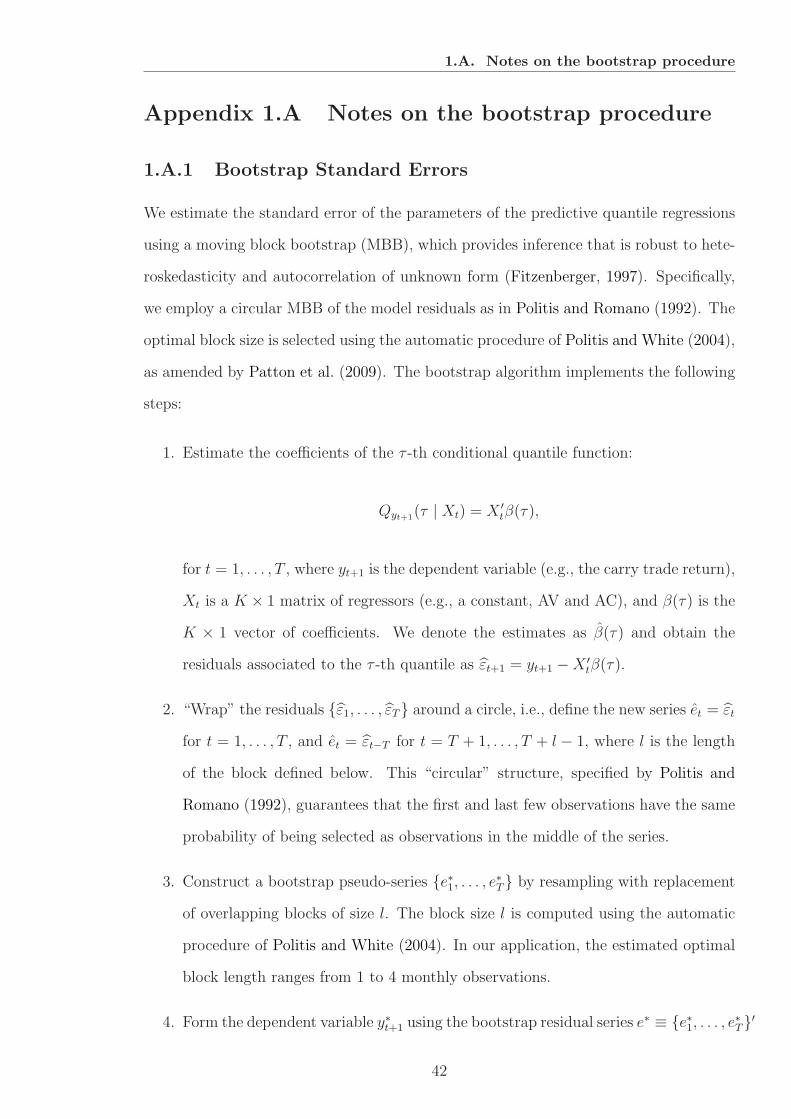
1.A. Notes on the bootstrap procedure
Appendix 1.A Notes on the bootstrap procedure
1.A.1 Bootstrap Standard Errors
We estimate the standard error of the parameters of the predictive quantile regressions
using a moving block bootstrap (MBB), which provides inference that is robust to hete-
roskedasticity and autocorrelation of unknown form (Fitzenberger, 1997). Specifically,
we employ a circular MBB of the model residuals as in Politis and Romano (1992). The
optimal block size is selected using the automatic procedure of Politis and White (2004),
as amended by Patton et al. (2009). The bootstrap algorithm implements the following
steps:
1. Estimate the coefficients of the τ -th conditional quantile function:
Qyt+1(τ | Xt) = X ′
tβ(τ),
for t = 1, . . . , T , where yt+1 is the dependent variable (e.g., the carry trade return),
Xt is a K × 1 matrix of regressors (e.g., a constant, AV and AC), and β(τ) is the
K × 1 vector of coefficients. We denote the estimates as β(τ) and obtain the
residuals associated to the τ -th quantile as εt+1 = yt+1 −X ′tβ(τ).
2. “Wrap” the residuals ε1, . . . , εT around a circle, i.e., define the new series et = εt
for t = 1, . . . , T , and et = εt−T for t = T + 1, . . . , T + l − 1, where l is the length
of the block defined below. This “circular” structure, specified by Politis and
Romano (1992), guarantees that the first and last few observations have the same
probability of being selected as observations in the middle of the series.
3. Construct a bootstrap pseudo-series e∗1, . . . , e∗T by resampling with replacement
of overlapping blocks of size l. The block size l is computed using the automatic
procedure of Politis and White (2004). In our application, the estimated optimal
block length ranges from 1 to 4 monthly observations.
4. Form the dependent variable y∗t+1 using the bootstrap residual series e∗ ≡ e∗1, . . . , e∗T
′
42

1.A. Notes on the bootstrap procedure
and the estimates β(τ) as follows:
y∗t+1 = X ′tβ(τ) + e∗t+1,
and then estimate the conditional quantile function Qy∗t+1(τ | Xt) = X ′
tβ(τ), ob-
taining the bootstrap estimate β∗(τ).
5. Repeat steps 3 and 4 for B = 10, 000 times. Denoting β∗j (τ) as the estimate of the
jth bootstrap, for j = 1, . . . , B, estimate the variance-covariance matrix of β(τ)
as follows:
Var(β(τ)
)=
1
B
B∑
j=1
(β∗j (τ)− β∗
j (τ))(β∗j (τ)− β∗
j (τ))′.
1.A.2 Bootstrap Hypothesis Testing
In order to test the null hypothesis of no predictability (i.e., β(τ) = 0), we perform a
double bootstrap to compute the bootstrap p-values (see, e.g., MacKinnon, 2007). The
procedure is as follows:
I. Obtain the estimate β(τ).
II. Obtain the estimate Var(β(τ)
)using the block bootstrap described above for
B2 = 500 bootstrap samples.
III. Compute the t-statistic for each coefficient βi(τ), i = 1, ..., K as follows:
ti =βi(τ)√
Var(βi(τ)
) .
IV. Generate B1 = 1, 000 bootstrap samples using the bootstrap DGP as in step 4
above, but this time imposing the null βi(τ) = 0. Use each of the new samples to
calculate β∗∗i,j(τ), j = 1, . . . , B1.
43

1.A. Notes on the bootstrap procedure
V. For each of the B1 bootstrap samples, perform steps II and III above in order to
generate B1 bootstrap test statistics t∗∗i,j.
VI. Calculate the bootstrap p-values for ti using
p∗i (ti) =1
B1
B1∑
j=1
I(|t∗∗i,j| > |ti|),
where I(·) denotes the indicator function, which is equal to 1 when its argument
is true and 0 otherwise.
44

1. Tables
Table 1.1. Exchange Rates
The table lists the 33 US dollar nominal exchange rates used to construct the FX market and carry
trade portfolios. The start date and end date of the data sample is shown for each exchange rate. The
transaction costs reported below are the median one-way proportional costs for the spot and forward
exchange rates, defined as half of the bid-ask spread divided by the mid rate, and are reported in basis
points. The transaction costs are computed using the longest bid and ask times series available for each
exchange rate for the sample range of January 1976 to February 2009.
Transaction Costs
Exchange Rate Start of Sample End of Sample Spot Forward
1 Australian Dollar December 1984 February 2009 5.42 7.31
2 Austrian Schilling January 1976 December 1998 7.64 11.08
3 Belgian Franc January 1976 December 1998 7.92 12.67
4 Canadian Dollar January 1976 February 2009 2.72 4.75
5 Czech Koruna January 1997 February 2009 5.97 6.75
6 Danish Krone January 1976 February 2009 4.16 7.03
7 Euro January 1999 February 2009 2.64 2.77
8 Finnish Markka January 1997 December 1998 6.52 5.28
9 French Franc January 1976 December 1998 4.98 7.56
10 German Mark January 1976 December 1998 8.09 15.55
11 Greek Drachma January 1997 December 2000 4.07 5.45
12 Hong Kong Dollar October 1983 February 2009 0.64 1.92
13 Hungarian Forint October 1997 February 2009 5.05 8.36
14 Indian Rupee October 1997 February 2009 3.13 4.39
15 Irish Punt January 1976 December 1998 4.70 9.00
16 Italian Lira January 1976 December 1998 3.16 8.54
17 Japanese Yen June 1978 February 2009 10.32 9.76
18 Mexican Peso January 1997 February 2009 4.35 5.25
19 Netherlands Guilder January 1976 December 1998 11.71 17.21
20 New Zealand Dollar December 1984 February 2009 8.14 10.44
21 Norwegian Krone January 1976 February 2009 4.65 7.29
22 Philippine Peso January 1997 February 2009 13.61 15.85
23 Polish Zloty February 2002 February 2009 6.52 7.41
24 Portuguese Escudo January 1976 December 1998 18.76 34.43
25 Saudi Arabian Riyal January 1997 February 2009 0.53 0.93
26 Singaporean Dollar December 1984 February 2009 3.14 6.94
27 South African Rand October 1983 February 2009 11.46 20.12
28 South Korean Won February 2002 February 2009 2.24 6.44
29 Spanish Peseta January 1976 December 1998 6.98 12.08
30 Swedish Krona January 1976 February 2009 4.85 7.76
31 Swiss Franc January 1976 February 2009 11.61 18.60
32 Taiwanese Dollar January 1997 February 2009 2.95 8.28
33 United Kingdom Pound January 1976 February 2009 2.67 3.54
45

1. Tables
Table 1.2. Descriptive Statistics
The table reports descriptive statistics for the monthly excess returns of two FX portfolios: the carry
trade and the market; for the two components of the carry trade: the exchange rate depreciation and
the interest rate differential; and for three monthly risk measures: market variance, average variance
and average correlation. The sample of 33 US dollar nominal exchange rates runs from January 1976
to February 2009. The return to the FX market portfolio is an equally weighted average of all exchange
rate excess returns. The carry trade portfolio is constructed every month by going long on the quintile
of currencies with the highest interest rates and going short on the bottom quintile. Market variance
is the variance of the monthly returns to the FX market portfolio. Average variance is the equally
weighted cross-sectional average of the monthly variances of all exchange rate excess returns. Average
correlation is the equally weighted cross-sectional average of the pairwise monthly correlations of all
exchange rate excess returns. The mean, standard deviation and the Sharpe ratio are annualized and
assume no transaction costs. AR(1) is the first order autocorrelation.
Panel A: Summary Statistics
Mean St. Dev. Sharpe Ratio Skewness Kurtosis AR(1)
Portfolio Returns
Carry Trade 0.086 0.078 1.092 −0.967 6.043 0.132
Market 0.010 0.078 0.131 −0.120 3.195 0.097
Carry Trade Components
Exchange Rate −0.051 0.079 −1.133 6.232 0.140
Interest Rate 0.137 0.023 2.506 15.578 0.655
Variances and Correlations
Market Variance 0.005 0.002 3.380 19.367 0.512
Average Variance 0.010 0.003 5.174 47.780 0.539
Average Correlation 0.477 0.182 0.028 2.241 0.796
Panel B: Cross-Correlations
Carry Market Market Average Average
Return Return Variance Variance Correlation
Portfolio Returns
Carry Trade Return 1.000
Market Return 0.091 1.000
Variances and Correlations
Market Variance −0.250 −0.145 1.000
Average Variance −0.371 −0.150 0.877 1.000
Average Correlation −0.048 −0.054 0.478 0.191 1.000
46

1. Tables
Table 1.3. Market Variance Decomposition
The table presents the ordinary least squares results for regressions on alternative decompositions of
the FX market variance. The dependent variable is the market variance defined as the variance of the
monthly returns to the FX market portfolio, which is an equally weighted average of the excess returns
of 33 US dollar nominal spot exchange rates. Average variance is the equally weighted cross-sectional
average of the variances of all exchange rate excess returns. Average correlation is the equally weighted
cross-sectional average of the pairwise correlations of all exchange rate excess returns. All variables
are contemporaneous and, with the exception of average correlation, they are annualized. Newey-West
(1987) t-statistics with five lags are reported in parentheses. The sample period runs from of January
1976 to February 2009.
Regressions for the Market Variance
(1) (2) (3) (4)Constant 0.000 −0.002 −0.004 0.000
(0.056) (−2.324) (−11.079) (1.473)
Average Variance 0.493 0.456(9.993) (13.883)
Average Correlation 0.015 0.010(8.960) (13.784)
(Average Variance)×(Average Correlation)
0.939(24.281)
R2(%) 76.8 23.5 86.8 93.0
47
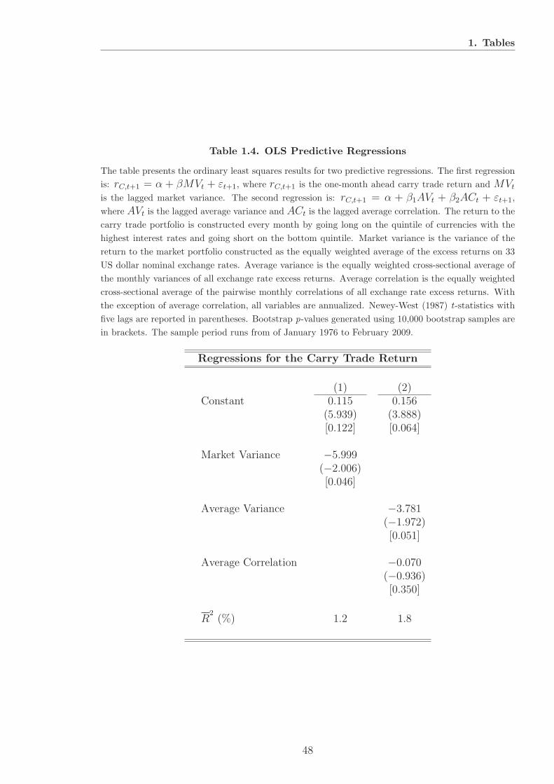
1. Tables
Table 1.4. OLS Predictive Regressions
The table presents the ordinary least squares results for two predictive regressions. The first regression
is: rC,t+1 = α + βMVt + εt+1, where rC,t+1 is the one-month ahead carry trade return and MVtis the lagged market variance. The second regression is: rC,t+1 = α + β1AVt + β2ACt + εt+1,
where AVt is the lagged average variance and ACt is the lagged average correlation. The return to the
carry trade portfolio is constructed every month by going long on the quintile of currencies with the
highest interest rates and going short on the bottom quintile. Market variance is the variance of the
return to the market portfolio constructed as the equally weighted average of the excess returns on 33
US dollar nominal exchange rates. Average variance is the equally weighted cross-sectional average of
the monthly variances of all exchange rate excess returns. Average correlation is the equally weighted
cross-sectional average of the pairwise monthly correlations of all exchange rate excess returns. With
the exception of average correlation, all variables are annualized. Newey-West (1987) t-statistics with
five lags are reported in parentheses. Bootstrap p-values generated using 10,000 bootstrap samples are
in brackets. The sample period runs from of January 1976 to February 2009.
Regressions for the Carry Trade Return
(1) (2)Constant 0.115 0.156
(5.939) (3.888)[0.122] [0.064]
Market Variance −5.999(−2.006)[0.046]
Average Variance −3.781(−1.972)[0.051]
Average Correlation −0.070(−0.936)[0.350]
R2(%) 1.2 1.8
48

1.Tables
Table 1.5. Market Variance
The table presents the regression results for the conditional quantile function: QrC,t+1(τ |MVt) = α (τ)+β (τ)MVt, where τ is a quantile of the one-month
ahead carry trade return rC,t+1 andMVt is the lagged market variance. The return to the carry trade portfolio is constructed every month by going long on the
quintile of currencies with the highest interest rates and going short on the bottom quintile. Market variance is the variance of the return to the market portfolio
constructed as the equally weighted average of the excess return on 33 US dollar nominal exchange rates. All variables are annualized. Bootstrap t-statistics
generated using 1,000 bootstrap samples are reported in parentheses. Bootstrap p-values using the double bootstrap are in brackets. The pseudo-R2is computed
as in Koenker and Machado (1999). The sample period runs from of January 1976 to February 2009.
Predictive Quantile Regressions for the Carry Trade Return
Quantile 0.05 0.1 0.2 0.3 0.4 0.5 0.6 0.7 0.8 0.9 0.95
Constant −0.024 −0.019 −0.005 0.003 0.007 0.011 0.015 0.020 0.025 0.034 0.044
(−6.227) (−4.742) (−2.100) (1.424) (4.711) (7.297) (8.886) (10.660) (17.106) (15.022) (15.569)
[0.000] [0.001] [0.058] [0.169] [0.001] [0.000] [0.000] [0.000] [0.000] [0.000] [0.000]
Market Variance −23.709 −4.473 −6.514 −6.691 −5.885 −5.358 −4.017 −3.206 −2.835 −5.588 −8.031
(−3.256) (−0.731) (−1.577) (−2.265) (−2.364) (−2.192) (−1.533) (−1.139) (−1.109) (−1.546) (−1.598)
[0.006] [0.495] [0.120] [0.042] [0.035] [0.039] [0.147] [0.296] [0.259] [0.132] [0.137]
R2(%) 0.9 0.4 0.4 0.8 1.1 0.5 −0.1 0.0 0.3 0.7 0.8
49
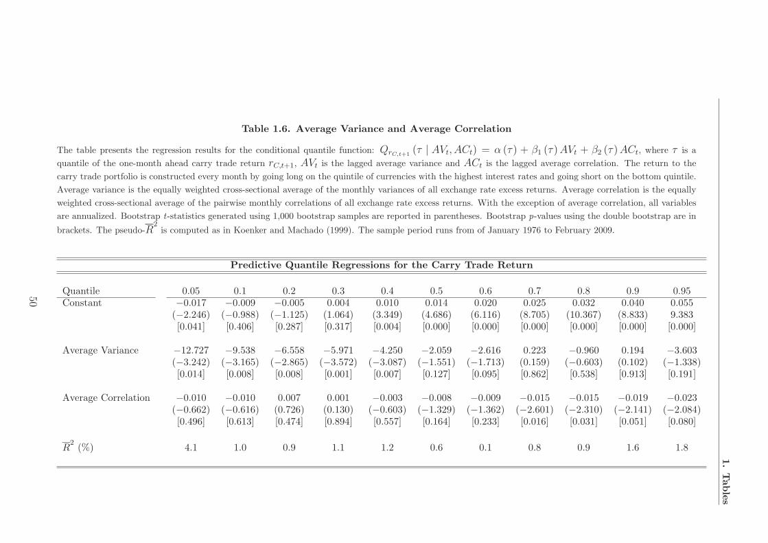
1.Tables
Table 1.6. Average Variance and Average Correlation
The table presents the regression results for the conditional quantile function: QrC,t+1(τ | AVt, ACt) = α (τ) + β1 (τ)AVt + β2 (τ)ACt, where τ is a
quantile of the one-month ahead carry trade return rC,t+1, AVt is the lagged average variance and ACt is the lagged average correlation. The return to the
carry trade portfolio is constructed every month by going long on the quintile of currencies with the highest interest rates and going short on the bottom quintile.
Average variance is the equally weighted cross-sectional average of the monthly variances of all exchange rate excess returns. Average correlation is the equally
weighted cross-sectional average of the pairwise monthly correlations of all exchange rate excess returns. With the exception of average correlation, all variables
are annualized. Bootstrap t-statistics generated using 1,000 bootstrap samples are reported in parentheses. Bootstrap p-values using the double bootstrap are in
brackets. The pseudo-R2is computed as in Koenker and Machado (1999). The sample period runs from of January 1976 to February 2009.
Predictive Quantile Regressions for the Carry Trade Return
Quantile 0.05 0.1 0.2 0.3 0.4 0.5 0.6 0.7 0.8 0.9 0.95Constant −0.017 −0.009 −0.005 0.004 0.010 0.014 0.020 0.025 0.032 0.040 0.055
(−2.246) (−0.988) (−1.125) (1.064) (3.349) (4.686) (6.116) (8.705) (10.367) (8.833) 9.383[0.041] [0.406] [0.287] [0.317] [0.004] [0.000] [0.000] [0.000] [0.000] [0.000] [0.000]
Average Variance −12.727 −9.538 −6.558 −5.971 −4.250 −2.059 −2.616 0.223 −0.960 0.194 −3.603(−3.242) (−3.165) (−2.865) (−3.572) (−3.087) (−1.551) (−1.713) (0.159) (−0.603) (0.102) (−1.338)[0.014] [0.008] [0.008] [0.001] [0.007] [0.127] [0.095] [0.862] [0.538] [0.913] [0.191]
Average Correlation −0.010 −0.010 0.007 0.001 −0.003 −0.008 −0.009 −0.015 −0.015 −0.019 −0.023(−0.662) (−0.616) (0.726) (0.130) (−0.603) (−1.329) (−1.362) (−2.601) (−2.310) (−2.141) (−2.084)[0.496] [0.613] [0.474] [0.894] [0.557] [0.164] [0.233] [0.016] [0.031] [0.051] [0.080]
R2(%) 4.1 1.0 0.9 1.1 1.2 0.6 0.1 0.8 0.9 1.6 1.8
50

1.Tables
Table 1.7. Additional Predictive Variables
The table presents the regression results for the conditional quantile function: QrC,t+1(τ | AVt, ACt, AIDt, rC,t) = α (τ) + β1 (τ)AVt + β2 (τ)ACt +
β3 (τ)AIDt + β4 (τ) rC,t, where τ is a quantile of the one-month ahead carry trade return rC,t+1, AVt is the lagged average variance, ACt is the lagged
average correlation, AIDt is the average interest rate differential and rC,t is the lagged carry trade return. The return to the carry trade portfolio is constructed
every month by going long on the quintile of currencies with the highest interest rates and going short on the bottom quintile. Average variance is the equally
weighted cross-sectional average of the monthly variances of all exchange rate excess returns. Average correlation is the equally weighted cross-sectional average
of the pairwise monthly correlations of all exchange rate excess returns. AID is the average interest rate differential of the quintile of currencies with the highest
interest rates minus the average interest rate differential of the quintile of currencies with the lowest interest rates. With the exception of average correlation,
all variables are annualized. Bootstrap t-statistics generated using 1,000 bootstrap samples are reported in parentheses. Bootstrap p-values using the double
bootstrap are in brackets. The pseudo-R2is computed as in Koenker and Machado (1999). The sample period runs from of January 1976 to February 2009.
Predictive Quantile Regressions for the Carry Trade Return
Quantile 0.05 0.1 0.2 0.3 0.4 0.5 0.6 0.7 0.8 0.9 0.95
Constant −0.013 −0.015 −0.009 −0.003 0.003 0.007 0.012 0.019 0.028 0.037 0.054
(−1.521) (−2.008) (−1.562) (−0.695) (1.075) (2.303) (3.176) (5.515) (7.979) (8.012) (7.882)
[0.162] [0.100] [0.185] [0.554] [0.252] [0.036] [0.007] [0.000] [0.000] [0.000] [0.000]
Average Variance −10.434 −5.689 −5.958 −5.457 −3.704 −4.086 −2.063 −2.720 −1.874 −0.735 −2.868
(−2.568) (−1.752) (−2.472) (−3.018) (−2.499) (−2.819) (−1.394) (−1.808) (−1.136) (−0.334) (−0.946)
[0.028] [0.090] [0.033] [0.007] [0.022] [0.010] [0.204] [0.079] [0.248] [0.736] [0.382]
Average Correlation −0.014 −0.012 −0.002 0.003 −0.004 −0.003 −0.006 −0.010 −0.016 −0.019 −0.026
(−0.972) (−0.961) (−0.181) (0.380) (−0.800) (−0.489) (−1.061) (−1.727) (−2.597) (−2.396) (−2.125)
[0.336] [0.428] [0.866] [0.722] [0.401] [0.611] [0.327] [0.102] [0.028] [0.039] [0.081]
Average Interest Differential −0.398 0.218 0.519 0.463 0.499 0.443 0.440 0.502 0.403 0.226 0.040
(−0.936) (0.583) (1.946) (2.372) (3.295) (2.978) (2.466) (3.032) (2.515) (0.956) (0.128)
[0.331] [0.622] [0.083] [0.042] [0.000] [0.007] [0.023] [0.004] [0.027] [0.339] [0.905]
Lagged Carry Return 0.255 0.296 0.154 0.101 0.089 0.067 0.035 0.015 −0.043 0.013 0.048
(1.892) (2.722) (2.002) (1.686) (1.953) (1.461) (0.663) (0.300) (−0.810) (0.193) (0.476)
[0.084] [0.021] [0.060] [0.128] [0.051] [0.153] [0.553] [0.749] [0.431] [0.853] [0.692]
R2(%) 4.8 3.1 2.1 2.4 2.9 2.0 1.1 1.6 1.1 1.6 1.4
51
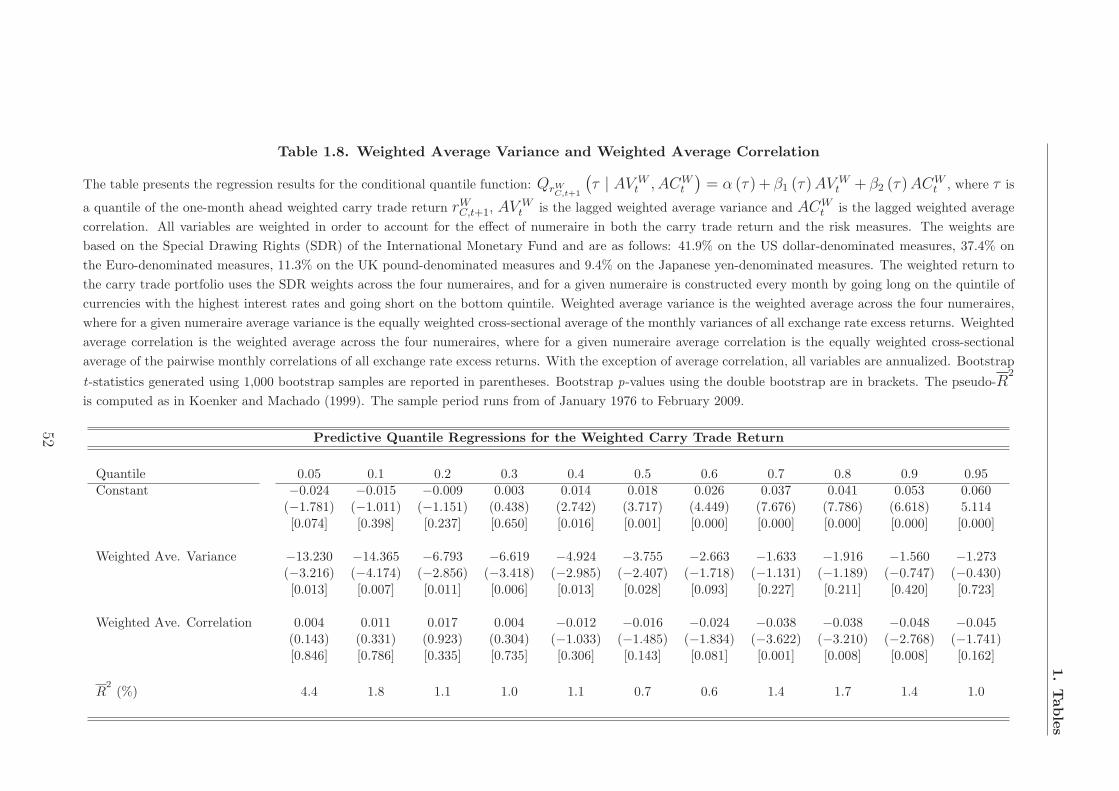
1.Tables
Table 1.8. Weighted Average Variance and Weighted Average Correlation
The table presents the regression results for the conditional quantile function: QrWC,t+1
(τ | AV W
t , ACWt
)= α (τ) + β1 (τ)AV
Wt + β2 (τ)AC
Wt , where τ is
a quantile of the one-month ahead weighted carry trade return rWC,t+1, AVWt is the lagged weighted average variance and ACW
t is the lagged weighted average
correlation. All variables are weighted in order to account for the effect of numeraire in both the carry trade return and the risk measures. The weights are
based on the Special Drawing Rights (SDR) of the International Monetary Fund and are as follows: 41.9% on the US dollar-denominated measures, 37.4% on
the Euro-denominated measures, 11.3% on the UK pound-denominated measures and 9.4% on the Japanese yen-denominated measures. The weighted return to
the carry trade portfolio uses the SDR weights across the four numeraires, and for a given numeraire is constructed every month by going long on the quintile of
currencies with the highest interest rates and going short on the bottom quintile. Weighted average variance is the weighted average across the four numeraires,
where for a given numeraire average variance is the equally weighted cross-sectional average of the monthly variances of all exchange rate excess returns. Weighted
average correlation is the weighted average across the four numeraires, where for a given numeraire average correlation is the equally weighted cross-sectional
average of the pairwise monthly correlations of all exchange rate excess returns. With the exception of average correlation, all variables are annualized. Bootstrap
t-statistics generated using 1,000 bootstrap samples are reported in parentheses. Bootstrap p-values using the double bootstrap are in brackets. The pseudo-R2
is computed as in Koenker and Machado (1999). The sample period runs from of January 1976 to February 2009.
Predictive Quantile Regressions for the Weighted Carry Trade Return
Quantile 0.05 0.1 0.2 0.3 0.4 0.5 0.6 0.7 0.8 0.9 0.95Constant −0.024 −0.015 −0.009 0.003 0.014 0.018 0.026 0.037 0.041 0.053 0.060
(−1.781) (−1.011) (−1.151) (0.438) (2.742) (3.717) (4.449) (7.676) (7.786) (6.618) 5.114[0.074] [0.398] [0.237] [0.650] [0.016] [0.001] [0.000] [0.000] [0.000] [0.000] [0.000]
Weighted Ave. Variance −13.230 −14.365 −6.793 −6.619 −4.924 −3.755 −2.663 −1.633 −1.916 −1.560 −1.273(−3.216) (−4.174) (−2.856) (−3.418) (−2.985) (−2.407) (−1.718) (−1.131) (−1.189) (−0.747) (−0.430)[0.013] [0.007] [0.011] [0.006] [0.013] [0.028] [0.093] [0.227] [0.211] [0.420] [0.723]
Weighted Ave. Correlation 0.004 0.011 0.017 0.004 −0.012 −0.016 −0.024 −0.038 −0.038 −0.048 −0.045(0.143) (0.331) (0.923) (0.304) (−1.033) (−1.485) (−1.834) (−3.622) (−3.210) (−2.768) (−1.741)[0.846] [0.786] [0.335] [0.735] [0.306] [0.143] [0.081] [0.001] [0.008] [0.008] [0.162]
R2(%) 4.4 1.8 1.1 1.0 1.1 0.7 0.6 1.4 1.7 1.4 1.0
52

1. Tables
Table 1.9. VIX, VXY and FX Risk Measures
The table presents ordinary least squares results for regressions of the VIX and VXY indices on monthly
FX risk measures. The VIX index is based on the 1-month model-free implied volatility of the S&P
500 equity index. The VXY index is based on the 3-month implied volatility of at-the-money-forward
options on the G-7 currencies. Market variance is the variance of the return to the market portfolio
constructed as the equally weighted average of the excess returns on 33 US dollar nominal exchange
rates. Average variance is the equally weighted cross-sectional average of the variances of exchange
rate excess returns. Average correlation is the equally weighted cross-sectional average of the pairwise
correlations of exchange rate excess returns. With the exception of average correlation, all variables
are annualized. Newey-West (1987) t-statistics with five lags are reported in parentheses. The sample
period for the VIX begins in January 1990 and for the VXY in January 1992. The sample period for
all indices ends in February 2009.
Panel A: Regressions for the VIX
(1) (2) (3) (4) (5)Constant 0.014 0.013 0.021 0.019 0.015
(13.962) (17.851) (16.058) (15.103) (15.302)
Market Variance 5.695(2.113)
Average Variance 3.556 4.003(6.559) (7.729)
Average Correlation −0.012 −0.016(−3.862) (−5.113)
(Average Variance)×(Average Correlation)
5.496(2.159)
R2(%) 13.5 24.7 6.9 37.6 12.4
Panel B: Regressions for the VXY
Constant 0.008 0.007 0.008 0.008 0.008(35.786) (30.391) (19.371) (19.868) (35.791)
Market Variance 3.305(10.540)
Average Variance 1.462 1.473(7.142) (6.869)
Average Correlation 0.001 −0.001(1.269) (−0.519)
(Average Variance)×(Average Correlation)
3.201(9.628)
R2(%) 53.0 54.5 0.5 54.4 49.6
53

1.Tables
Table 1.10. VIX and VXY
The table presents the regression results for two conditional quantile functions. The first one is: QrC,t+1(τ | V IXt) = α (τ) + β (τ)V IXt, where τ is a
quantile of the one-month ahead carry trade return rC,t+1 and V IXt is the lagged VIX index. The second one is: QrC,t+1(τ | V XYt) = α (τ)+β (τ)V XYt,
where V XYt is the lagged VXY index. The return to the carry trade portfolio is constructed every month by going long on the quintile of currencies with
the highest interest rates and going short on the bottom quintile. The VIX index is based on the 1-month model-free implied volatility of the S&P 500 equity
index. The VXY index is based on the 3-month implied volatility of at-the-money-forward options on the G-7 currencies. All variables are annualized. Bootstrap
t-statistics generated using 1,000 bootstrap samples are reported in parentheses. Bootstrap p-values using the double bootstrap are in brackets. The pseudo-R2
is computed as in Koenker and Machado (1999). The sample period runs from of January 1976 to February 2009.
Panel A: The Carry Trade Return on VIX
Quantile 0.05 0.1 0.2 0.3 0.4 0.5 0.6 0.7 0.8 0.9 0.95Constant −0.018 −0.021 −0.004 0.004 0.004 0.009 0.014 0.016 0.019 0.025 0.023
(−1.382) (−1.875) (−0.507) (0.686) (0.929) (2.013) (3.670) (3.576) (4.077) (3.972) (3.521)[0.195] [0.097] [0.621] [0.464] [0.359] [0.090] [0.003] [0.006] [0.003] [0.001] [0.006]
VIX −0.103 −0.027 −0.023 −0.018 0.006 0.008 −0.001 0.015 0.023 0.026 0.070(−1.620) (−0.511) (−0.580) (−0.605) (0.283) (0.379) (−0.029) (0.731) (1.057) (0.870) (1.988)[0.140] [0.605] [0.584] [0.511] [0.745] [0.699] [0.957] [0.520] [0.341] [0.444] [0.065]
R2(%) 0.8 −0.2 −0.2 −0.3 −0.4 −0.4 −0.4 −0.2 0.2 0.1 2.1
Panel B: The Carry Trade Return on VXY
Constant −0.051 −0.028 0.003 0.009 0.012 0.023 0.028 0.039 0.027 0.041 0.024(−1.646) (−1.660) (0.241) (0.953) (1.347) (2.379) (3.239) (4.258) (3.093) (4.029) (1.414)[0.150] [0.098] [0.795] [0.356] [0.199] [0.028] [0.004] [0.001] [0.010] [0.003] [0.173]
VXY 0.183 0.073 −0.096 −0.102 −0.082 −0.123 −0.140 −0.190 0.005 −0.081 0.160(0.628) (0.447) (−0.777) (−1.139) (−0.959) (−1.354) (−1.704) (−2.209) (0.061) (−0.828) (0.956)[0.591] [0.615] [0.439] [0.282] [0.355] [0.185] [0.105] [0.044] [0.916] [0.373] [0.352]
R2(%) −0.2 −0.2 0.1 0.1 0.4 1.0 1.0 0.4 −0.5 −0.3 1.2
54

1. Tables
Table 1.11. Out-of-Sample Augmented Carry Trade Strategies
The table presents the out-of-sample performance of augmented carry trade strategies that condition
on the movement of average variance and/or average correlation with and without transaction costs.
Panel A assumes no transaction costs, whereas Panel B implements the carry trade strategies using the
transaction costs listed in Table 1. Average variance is the equally weighted cross-sectional average of
the monthly variances of all exchange rate excess returns. The average variance strategy implements
the following rule at each time t : for the carry trade returns that are lower than the τ -quantile of the
distribution, if average variance has increased from t-1 to t, we close the carry trade positions and thus
receive a return of zero at t+1; otherwise we execute the standard carry trade. Average correlation is
the equally weighted cross-sectional average of the pairwise monthly correlations of all exchange rate
excess returns. The average correlation strategy implements the following rule at each time t : for
the carry trade returns that are higher than the 1−τ quantile, if average correlation has decreased
from t-1 to t, we double the carry trade positions and thus receive twice the carry return at t+1;
otherwise we execute the standard carry trade. The combined average variance and average correlation
strategy makes the following decision at each time t : for the carry trade returns that are lower than
the τ -quantile, if average variance has increased from t-1 to t, we close the carry trade positions and
thus receive a return of zero; and for the carry trade returns that are higher than the 1−τ quantile,
if average correlation has decreased from t-1 to t, we double the carry trade positions and thus receive
twice the carry return; otherwise we execute the standard carry trade. The mean, standard deviation
and Sharpe ratio are reported in annualized terms. The turnover ratio is equal to the percentage of
the currencies that on average are traded every month. The sample period runs from of January 1976
to February 2009. All strategies move forward recursively starting 3 years after the beginning of the
sample so that the first observation is for January 1979.
Panel A: No Transaction Costs
Carry Trade Average Variance Strategy
Quantile 0.1 0.2 0.3 0.4 0.5 0.6 0.7 0.8 0.9
Mean 0.084 0.094 0.091 0.085 0.079 0.073 0.069 0.066 0.059 0.054
St. Dev. 0.079 0.071 0.069 0.066 0.065 0.064 0.061 0.060 0.057 0.056
Sharpe ratio 1.070 1.314 1.326 1.279 1.213 1.142 1.120 1.098 1.022 0.968
Turnover 0.171 0.208 0.264 0.310 0.346 0.387 0.421 0.444 0.485 0.514
Average Correlation Strategy
Mean 0.084 0.146 0.147 0.139 0.130 0.122 0.118 0.114 0.107 0.097
St. Dev. 0.079 0.121 0.115 0.111 0.107 0.104 0.100 0.096 0.091 0.085
Sharpe ratio 1.070 1.208 1.284 1.262 1.212 1.174 1.186 1.186 1.182 1.134
Turnover 0.171 0.557 0.511 0.454 0.412 0.370 0.340 0.294 0.252 0.214
Combined Average Variance and Average Correlation Strategy
Mean 0.084 0.104 0.106 0.107 0.106 0.099
St. Dev. 0.079 0.095 0.092 0.088 0.084 0.081
Sharpe ratio 1.070 1.095 1.152 1.211 1.264 1.224
Turnover 0.171 0.589 0.522 0.440 0.352 0.257
(continued)
55

1. Tables
Panel B: With Transaction Costs
Carry Trade Average Variance Strategy
Quantile 0.1 0.2 0.3 0.4 0.5 0.6 0.7 0.8 0.9
Mean 0.058 0.070 0.068 0.062 0.058 0.055 0.053 0.050 0.043 0.040
St. Dev. 0.079 0.071 0.069 0.066 0.065 0.063 0.061 0.060 0.057 0.055
Sharpe ratio 0.741 0.977 0.983 0.941 0.892 0.866 0.869 0.836 0.761 0.729
Turnover 0.171 0.208 0.259 0.306 0.344 0.385 0.417 0.442 0.485 0.513
Average Correlation Strategy
Mean 0.058 0.109 0.109 0.107 0.097 0.091 0.090 0.085 0.079 0.070
St. Dev. 0.079 0.121 0.115 0.111 0.107 0.103 0.099 0.095 0.090 0.085
Sharpe ratio 0.741 0.903 0.949 0.971 0.913 0.881 0.904 0.891 0.876 0.823
Turnover 0.171 0.557 0.513 0.458 0.411 0.375 0.341 0.296 0.252 0.215
Combined Average Variance and Average Correlation Strategy
Mean 0.058 0.081 0.082 0.081 0.080 0.074
St. Dev. 0.079 0.094 0.091 0.088 0.084 0.081
Sharpe ratio 0.741 0.853 0.895 0.926 0.959 0.914
Turnover 0.171 0.594 0.521 0.438 0.347 0.259
56
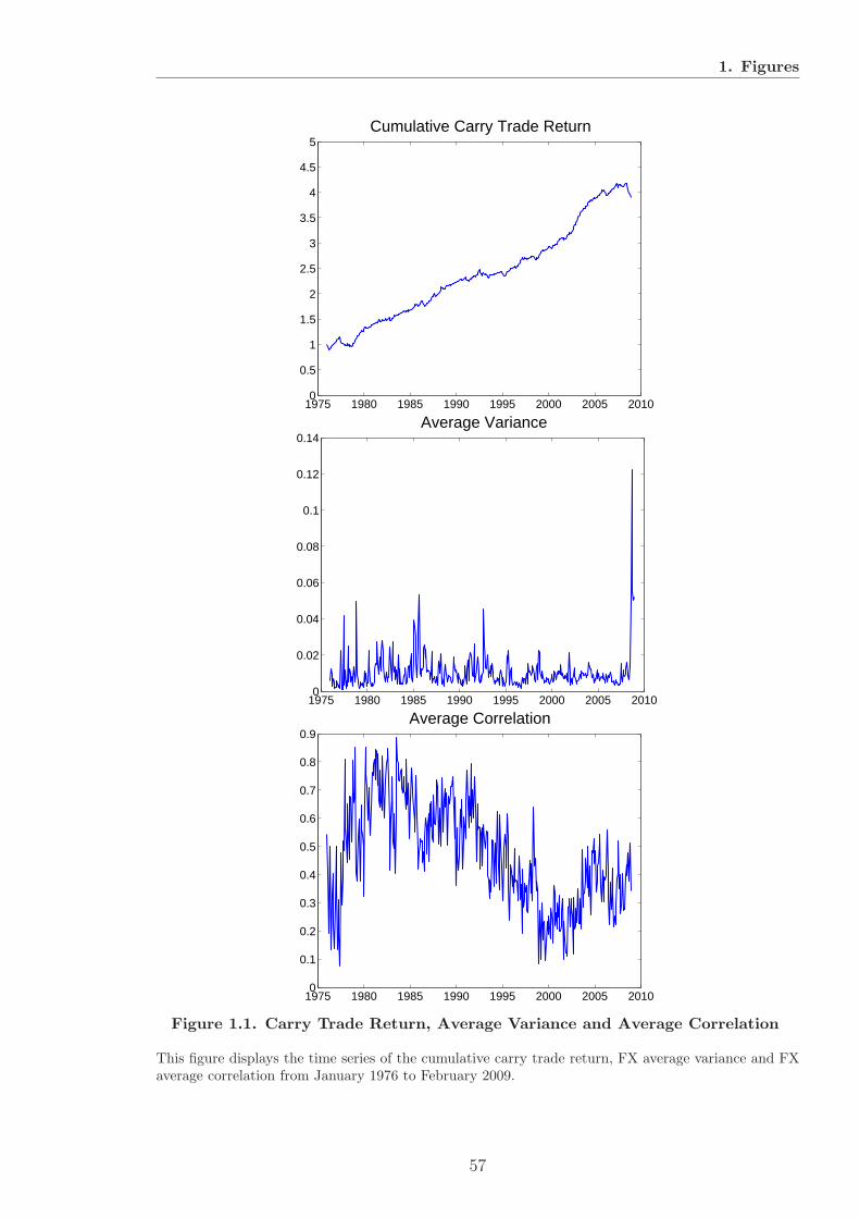
1. Figures
1975 1980 1985 1990 1995 2000 2005 20100
0.5
1
1.5
2
2.5
3
3.5
4
4.5
5Cumulative Carry Trade Return
1975 1980 1985 1990 1995 2000 2005 20100
0.02
0.04
0.06
0.08
0.1
0.12
0.14Average Variance
1975 1980 1985 1990 1995 2000 2005 20100
0.1
0.2
0.3
0.4
0.5
0.6
0.7
0.8
0.9Average Correlation
Figure 1.1. Carry Trade Return, Average Variance and Average Correlation
This figure displays the time series of the cumulative carry trade return, FX average variance and FXaverage correlation from January 1976 to February 2009.
57

1. Figures
0.050.1 0.2 0.3 0.4 0.5 0.6 0.7 0.8 0.90.95−0.04
−0.03
−0.02
−0.01
0
0.01
0.02
0.03
0.04
0.05Constant
Quantile
α
0.050.1 0.2 0.3 0.4 0.5 0.6 0.7 0.8 0.90.95−40
−35
−30
−25
−20
−15
−10
−5
0
5
10Market Variance
Quantile
β
Figure 1.2. Market Variance
This figure shows the parameter estimates of the predictive quantile regression of the one-month-aheadcarry trade return on the lagged market variance. The dashed lines indicate the 95% confidence intervalbased on bootstrap standard errors.
58

1. Figures
0.050.1 0.2 0.3 0.4 0.5 0.6 0.7 0.8 0.90.95−0.04
−0.02
0
0.02
0.04
0.06
0.08Constant
Quantile
α
0.050.1 0.2 0.3 0.4 0.5 0.6 0.7 0.8 0.90.95−25
−20
−15
−10
−5
0
5Average Variance
Quantile
β 1
0.050.1 0.2 0.3 0.4 0.5 0.6 0.7 0.8 0.90.95−0.05
−0.04
−0.03
−0.02
−0.01
0
0.01
0.02
0.03Average Correlation
Quantile
β 2
Figure 1.3. Average Variance and Average Correlation
This figure illustrates the parameter estimates of the predictive quantile regression of the one-month-ahead carry trade return on the lagged average variance and average correlation. The dashed linesindicate the 95% confidence interval based on bootstrap standard errors.
59
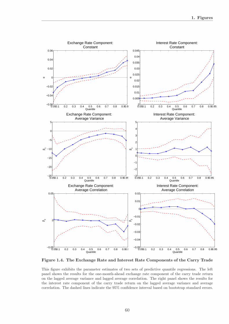
1. Figures
0.050.1 0.2 0.3 0.4 0.5 0.6 0.7 0.8 0.90.95−0.06
−0.04
−0.02
0
0.02
0.04
0.06
Exchange Rate Component:Constant
Quantile
α
0.050.1 0.2 0.3 0.4 0.5 0.6 0.7 0.8 0.90.95−25
−20
−15
−10
−5
0
5
Exchange Rate Component:Average Variance
Quantile
β 1
0.050.1 0.2 0.3 0.4 0.5 0.6 0.7 0.8 0.90.95−0.05
0
0.05
Exchange Rate Component:Average Correlation
Quantile
β 2
0.050.1 0.2 0.3 0.4 0.5 0.6 0.7 0.8 0.90.950
0.005
0.01
0.015
0.02
0.025
0.03
0.035
0.04
0.045
Interest Rate Component:Constant
Quantile
α
0.050.1 0.2 0.3 0.4 0.5 0.6 0.7 0.8 0.90.95−3
−2
−1
0
1
2
3
4
5
Interest Rate Component:Average Variance
Quantile
β 1
0.050.1 0.2 0.3 0.4 0.5 0.6 0.7 0.8 0.90.95−0.05
−0.04
−0.03
−0.02
−0.01
0
0.01
0.02
Interest Rate Component:Average Correlation
Quantile
β 2
Figure 1.4. The Exchange Rate and Interest Rate Components of the Carry Trade
This figure exhibits the parameter estimates of two sets of predictive quantile regressions. The leftpanel shows the results for the one-month-ahead exchange rate component of the carry trade returnon the lagged average variance and lagged average correlation. The right panel shows the results forthe interest rate component of the carry trade return on the lagged average variance and averagecorrelation. The dashed lines indicate the 95% confidence interval based on bootstrap standard errors.
60

1. Figures
0.050.1 0.2 0.3 0.4 0.5 0.6 0.7 0.8 0.90.95−0.04
−0.02
0
0.02
0.04
0.06
0.08Constant
Quantile
α
0.050.1 0.2 0.3 0.4 0.5 0.6 0.7 0.8 0.90.95−20
−15
−10
−5
0
5Average Variance
Quantile
β 1
0.050.1 0.2 0.3 0.4 0.5 0.6 0.7 0.8 0.90.95−0.05
−0.04
−0.03
−0.02
−0.01
0
0.01
0.02Average Correlation
Quantile
β 2
0.050.1 0.2 0.3 0.4 0.5 0.6 0.7 0.8 0.90.95−1.5
−1
−0.5
0
0.5
1
1.5Interest differential
Quantile
β 3
0.050.1 0.2 0.3 0.4 0.5 0.6 0.7 0.8 0.90.95−0.2
−0.1
0
0.1
0.2
0.3
0.4
0.5
0.6Lagged Carry Return
Quantile
β 4
Figure 1.5. Additional Predictive Variables
This figure illustrates the parameter estimates of the predictive quantile regression of the one-month-ahead carry trade return on the lagged average variance, lagged average correlation and two additionalpredictive variables: the interest rate differential and the lagged carry trade return. The dashed linesindicate the 95% confidence interval based on bootstrap standard errors.
61

1. Figures
0.050.1 0.2 0.3 0.4 0.5 0.6 0.7 0.8 0.90.95−0.06
−0.04
−0.02
0
0.02
0.04
0.06
0.08Constant
Quantile
α
0.050.1 0.2 0.3 0.4 0.5 0.6 0.7 0.8 0.90.95−25
−20
−15
−10
−5
0
5
10Weighted Average Variance
Quantile
β 1
0.050.1 0.2 0.3 0.4 0.5 0.6 0.7 0.8 0.90.95−0.1
−0.08
−0.06
−0.04
−0.02
0
0.02
0.04
0.06
0.08Weighted Average Correlation
Quantile
β 2
Figure 1.6. The Numeraire Effect
This figure displays the parameter estimates of the predictive quantile regression of the weighted one-month-ahead carry trade return on the lagged weighted average variance and lagged weighted averagecorrelation. The weighted variables account for the numeraire effect using the IMF weights for SpecialDrawing Rights: 41.9% on the US dollar, 37.4% on the Euro, 11.3% on the UK pound and 9.4% onthe Japanese yen. The dashed lines indicate the 95% confidence interval based on bootstrap standarderrors.
62

1. Figures
0.050.1 0.2 0.3 0.4 0.5 0.6 0.7 0.8 0.90.95−0.05
−0.04
−0.03
−0.02
−0.01
0
0.01
0.02
0.03
0.04Constant
Quantile
α
0.050.1 0.2 0.3 0.4 0.5 0.6 0.7 0.8 0.90.95−0.25
−0.2
−0.15
−0.1
−0.05
0
0.05
0.1
0.15VIX
Quantile
β
0.050.1 0.2 0.3 0.4 0.5 0.6 0.7 0.8 0.90.95−0.12
−0.1
−0.08
−0.06
−0.04
−0.02
0
0.02
0.04
0.06
0.08Constant
Quantile
α
0.050.1 0.2 0.3 0.4 0.5 0.6 0.7 0.8 0.90.95−0.6
−0.4
−0.2
0
0.2
0.4
0.6
0.8VXY
Quantile
β
Figure 1.7. VIX and VXY
This figure exhibits the parameter estimates of two sets of predictive quantile regressions. The leftpanel shows the results for the one-month-ahead carry trade return on the lagged VIX index. The rightpanel shows the results for the one-month-ahead carry trade return on the lagged VXY index. Thedashed lines indicate the 95% confidence interval based on bootstrap standard errors.
63

1. Figures
1975 1980 1985 1990 1995 2000 2005 2010−0.4
−0.3
−0.2
−0.1
0
0.1
0.2
0.3
Figure 1.8. Conditional Skewness
This figure shows the time-variation of the robust conditional skewness measure of Kim and White(2004) based on the predictive quantile regressions. The measure uses the inter-quartile range (a =0.25).
64

Chapter 2
On the evolution of the exchange
rate response to fundamental shocks
2.1 Introduction
In a frictionless and risk-neutral economy, asset prices should react instantaneously
to fundamental shocks to ensure that expected excess returns are zero. In the case
of the foreign exchange market, this implies that a sudden increase in interest rate
differentials should lead to an impact appreciation of the high-interest currency, followed
by a depreciation so that uncovered interest rate parity (UIP) holds. A carry trader, who
invests in a high-interest currency (the investment currency) by funding her position
in a low-interest currency (the funding currency), would therefore face only an impact
positive excess return, but this would then become zero on average as implied by UIP.
However, empirical evidence seems to be at odds with the exchange rate behaviour
outlined above. The “forward premium puzzle” implies that UIP is systematically viola-
ted as future currency excess returns are predictable (Fama, 1984; Bilson, 1981; Engel,
1996), and that carry trade strategies tend to be profitable (Della Corte et al. 2009,
Burnside et al. 2011). These results violate unconditional UIP—the response of the
exchange rate to all shocks on average. Moreover, UIP is also violated conditionally :
conditional on monetary policy shocks, cumulative excess returns on foreign exchange
65

2.1. Introduction
tend to be sizable and persistent.1 This latter evidence has been studied in much of
the literature on the “delayed overshooting puzzle”: contractionary monetary policy
shocks lead to a persistent appreciation of the domestic currency before starting to
depreciate (Eichenbaum and Evans, 1995; Scholl and Uhlig, 2008). These dynamics
stand in stark contrast with Dornbusch (1976) classical hypothesis of an immediate ap-
preciation and subsequent persistent depreciation following a monetary policy shock, a
hypothesis which follows from the assumption of UIP and long-run purchasing power
parity (PPP). Similarly, Brunnermeier et al. (2009) find that exchange rates initially
underreact to interest rate differential shocks: when the foreign interest rate increases
relative to the domestic interest rate, the investment currency appreciates sluggishly,
with cumulative excess returns reaching the level implied by UIP and PPP only after a
few quarters. At longer horizons, instead, they find evidence of possible overreaction of
the exchange rate to interest rate differential shocks.
This chapter re-examines these issues in light of the recent literature on nonlinea-
rities in the foreign exchange market. I do not consider UIP and PPP in general, but
conditional on interest rate differential shocks. Previous studies that document sizable
conditional excess returns (violating UIP) and a sluggish reaction of the exchange rate
do not generally consider the possibility that either or both the volatility of the shocks
and the transmission mechanism may have changed over time. Therefore, previous re-
sults may not reflect the current state of the economy but just an average over the past.
Given a simple present-value model for the currency excess return which assumes UIP
and long-run PPP,2 the research questions are therefore the following: how large the
deviations from the present value of future fundamentals3 should one expect following
an interest rate shock, given the current state of the economy? Do these conditional
deviations converge to the level implied by fundamentals, and, if so, how does this
1In distinguishing between unconditional and conditional UIP violations, I follow Faust and Rogers(2003) and Scholl and Uhlig (2008).
2The present-value approach adopted in this chapter is inspired by e.g. Froot and Ramadorai (2005),Brunnermeier et al. (2009), Engel (2010), and Engel and West (2010).
3In this chapter, I consider as fundamentals only those strictly implied by the assumptions of UIPand long-run PPP, i.e. real interest rate differentials, as discussed in Section 2.2. Therefore, I do notconsider other “classic” fundamentals such as relative money supplies and outputs, as in e.g. Engel andWest (2005).
66
2.1. Introduction
behaviour evolve over time as the state of the economy changes?
A number of previous studies have already documented how nominal and real ex-
change rate dynamics may have changed over time. Moreover, these studies have shown
how allowing for nonlinearities may shed light, and possibly explain, apparent devia-
tions from the parity relations which form the basis of much of the international finance
literature—namely, UIP and PPP. For example, Taylor et al. (2001) show that real
exchange rates (or equivalently, PPP deviations) are well characterized by a nonlinear
mean-reverting processes leading to time-varying half-lives in which larger shocks mean-
revert much faster than those previously reported for linear models, therefore potentially
explaining the PPP puzzle (Rogoff, 1996). Sarno et al. (2006) find that deviations from
UIP display significant nonlinearities, consistent with theories based on transaction costs
(e.g. Dumas, 1992) or limits to speculation (Lyons, 2001). This evidence leads them
to conclude that UIP deviations may be less indicative of major market inefficiencies
than previously thought. Christiansen et al. (2011) show that carry trade returns dis-
play time-varying risk exposure to the stock and bond markets depending on switching
regimes characterized by the level of foreign exchange volatility. Mumtaz and Sunder-
Plassmann (2010) find that the transmission of demand, supply and nominal shocks on
the real exchange rate displays significant time variation, with an increasing impact of
demand shocks over the years. However, none of these studies analyse the evolution of
conditional violations of UIP over time.
Therefore, the importance of analysing nonlinearities in exchange rate dynamics
seems to be undisputed. Similarly to the empirical studies above, I approximate non-
linearities by allowing for time variation in the parameters linking fundamentals to
exchange rates.4 In the context of this chapter, in which I analyse conditional violations
of UIP, this translates into estimating the time-varying impulse response functions of
the currency excess return to interest rate differential shocks. A natural framework to
estimate these impulse responses is to use a Bayesian time-varying-parameters vector-
4Bacchetta and van Wincoop (2004, 2010) provide a theory of exchange rate determination whichrationalizes parameter instability in empirical exchange rate models. They show that foreign exchangemarket participants can optimally choose to change the weight attached to different economic funda-mentals in the context of rational expectation models.
67
2.2. Foreign Exchange Excess Returns
autoregression (TVP-VAR) with stochastic volatility. Particularly, I adopt the metho-
dology from recent advances in the macroeconometric literature which has fruitfully
applied this technique in other contexts, see e.g. Cogley and Sargent (2005), Primiceri
(2005), Benati (2008), and Mumtaz and Sunder-Plassmann (2010).5 Allowing for time
variation both in the VAR coefficients and the covariance matrix leaves it up to the data
to determine whether the time variation of the linear structure derives from changes in
the size of the shocks (impulse) or from changes in the propagation mechanism (res-
ponse).
I provide empirical evidence that the transmission of the interest rate differential
shocks has changed over time. However, even if to a varying degree over the years, some
of the puzzling results previously documented with linear models remain. I show that
currency excess returns tend to initially underreact to interest rate differential shocks
for the whole sample considered, undershooting the level implied by UIP and long-run
PPP. At longer horizons, the previously documented evidence of overshooting tends to
disappear in recent years in the case of the euro, the British pound and the Canadian
dollar. Instead, overreaction at long horizons is a persistent feature of the excess returns
on the Japanese yen and the Swiss franc throughout the whole sample.
These results suggest that previously documented conditional violations of UIP may
have secularly declined over time, at least for the euro, the British pound and the
Canadian dollar. However, the results for the Japanese yen and the Swiss franc—two
currencies which have been traditionally used for funding carry trade positions—may
hint that speculation in the foreign exchange market may constitute a destabilizing
force, driving exchange rates away from fundamentals.
2.2 Foreign Exchange Excess Returns
The objective of this chapter is to study the evolution over time of conditional deviations
from UIP, i.e. the reaction of currency excess returns to an unexpected shock to interest
5See also Koop and Korobilis (2010) for a recent survey of the methodologies used in this chapter.
68

2.2. Foreign Exchange Excess Returns
rate differentials. Therefore, we first need to to compute the level of the unexpected
excess return that would be predicted under the assumption of UIP. By definition, the
log excess return on foreign exchange is equal to the interest rate differential plus the
appreciation rate of the foreign currency
zt = i∗t−1 − it−1 + (st − st−1), (2.1)
where st is the natural logarithm of the exchange rate (defined as the domestic price of
foreign currency, so that an increase in st denotes appreciation of the foreign currency),
and it and i∗t are the continuously compounded domestic and foreign riskless interest
rates, respectively. In terms of the log real exchange rate, defined as qt = st + p∗t − pt
where p∗t and pt are the logs of the foreign and domestic price levels, Equation (2.1) can
be rewritten as
zt+1 = (i∗t − π∗t+1)− (it − πt+1) + (qt+1 − qt), (2.2)
where π∗t+1 and πt+1 are the foreign and domestic inflation rates. Assuming UIP, the ex-
pected excess return for a risk-neutral investor should be equal to zero, i.e., Etzt+j = 0,
implying that an interest rate differential gain from borrowing abroad and lending do-
mestically should be offset by the expected appreciation rate of the foreign currency. As
in Froot and Ramadorai (2005) and Brunnermeier et al. (2009), I also make the relati-
vely milder assumption that long-run PPP holds in expectation, i.e. limj→∞Etqt+j = 0.
We can now solve Equation (2.2) forward and, by taking the expectation conditional on
time-t information, we have
qt =∞∑
i=1
Et[(i∗t+i−1 − π∗
t+i)− (it+i−1 − πt+i)]. (2.3)
Therefore, under UIP and long-run PPP, an increase in expected future real interest rate
differentials should be reflected in a real appreciation of the foreign currency. Following
a surprise increase in foreign interest rates relative to the domestic ones (i.e. i∗t+1−it+1−
Et[i∗t+1 − it+1] > 0), we can use Equation (2.3) together with the definition of excess
return in Equation (2.2) in order to express the unexpected one-period excess return as
69

2.3. Empirical Approach
the sum of all future innovations in expected future real interest differentials:
zt+1 − Etzt+1 =∞∑
i=1
[Et+1(i
∗t+i − it+i)− Et(i
∗t+i − it+i)
−(Et+1(π
∗t+i+1 − πt+i+1)− Et(π
∗t+i+1 − πt+i+1)
)]. (2.4)
Note also that, under UIP, Etzt+1 = 0, so that (zt+1 − Etzt+1) = zt+1. Therefore, UIP
predicts that a higher foreign interest rate leads to a jump in the excess return which
reflects the present value of changes in expectations of future fundamentals. At longer
horizons (i.e. after the unexpected shock) UIP also implies that the cumulative return
should remain flat, as the expected future interest rate differentials are exactly offset
by exchange rate depreciations. The present value in Equation (2.4) can be estimated
using standard results (see e.g. Campbell, 1991, and Hamilton, 1994) using the long-run
responses of a VAR which includes i∗t − it, π∗t − πt, and zt.
Comparing this present value to the actual cumulative response of the excess return
to interest rate differential shocks, Brunnermeier et al. (2009) find that exchange rates
initially underreact to the interest rate differential shock for all the currencies conside-
red: when the foreign interest rate increases relative to the domestic interest rate, the
investment currency appreciates sluggishly, with cumulative excess returns reaching the
level implied by UIP and PPP only after a few quarters.
2.3 Empirical Approach
2.3.1 Model
I analyse the evolution over time of the deviations from UIP conditional on interest rates
shocks as implied by the present-value relationship in Equation (2.4), and re-examine
the results obtained by the previous literature (especially Brunnermeier et al., 2009).
A natural way to do so is to allow for the parameters of the VAR used in the
estimation of Equation (2.4) to vary over time, and then compare the UIP-implied levels
of the unexpected excess return shock to the actual (time-varying) impulse responses.
70

2.3. Empirical Approach
However, as noted by Sims (2001) and Stock (2001), the possible presence of time-
varying covariance matrix in the dynamics of the variables considered may incorrectly
inflate the time-variation of the coefficients of a TVP-VAR which does not explicitly
take this into account.
Therefore, I use the TVP-VAR model proposed by Primiceri (2005), which allows
for time-variation both in the coefficients and in the covariance matrix of the VAR
innovations. As stressed by Primiceri (2005), this feature of the model leaves it up
to the data to determine whether the time variation of the linear structure derives
from changes in the size of the shocks (impulse) or from changes in the propagation
mechanism (response).
I specify a time-varying parameter VAR(p) with stochastic volatility as follows:
yt = B0,t +
p∑
j=1
Bj,tyt−j + ǫt, (2.5)
where
yt =
i∗t − it
π∗t − πt
zt
,
with i∗t −it being the interest rate differential, π∗t −πt being the inflation rate differential,
and zt being the excess return on foreign exchange as defined in Equation (2.1). The
vector ǫt includes heteroskedastic unobservable shocks with covariance matrix Ωt. Using
the Bayesian Information Criterion with quarterly data, I set the number of lags p equal
to 1. Following Cogley and Sargent (2001, 2005) and Benati (2008), I model the time-
varying parameters as driftless random walks subject to reflecting barriers to ensure
the stability of the VAR system. Let βt denote the vector stacking all right-hand-
side coefficients of Equation (2.5), and let βT = β′1, . . . , β
′T
′, then the joint prior
distribution of the VAR coefficients is
p(βT , Q) ∝ I(βT )f(Q)f(βT |β0, Q) = I(βT )f(Q)T∏
t=1
p(βt|βt−1, Q), (2.6)
71

2.3. Empirical Approach
where
βt+1|βt, Q ∼ N(βt, Q). (2.7)
The reflecting barrier I(βT ) =∏T
s=1 I(βs) ensures the stability of the system by using
the indicator function I(βs) which takes a value of zero when the roots of the associated
VAR polynomials are inside the unit circle, and it is equal to one otherwise.
Following Primiceri (2005), I model the conditional covariance matrix Ωt of the
reduced-form innovations in Equation (2.5) using the following decomposition:
AtΩtA′t = ΣtΣ
′t, (2.8)
where Σt is a diagonal matrix with diagonal elements σj,t, that is
Σt =
σ1,t 0 . . . . 0
0 σ2,t . . . . .
. . . . . . .
0 . . . . 0 σM,t
, (2.9)
and At is the lower triangular matrix
At =
1 0 . . . . 0
a21,t 1 . . . . .
. . . . . . .
. . . . . 1 0
aM1,t . . . . aM(M−1),t 1
, (2.10)
which captures the time variation of the simultaneous interactions among the M va-
riables in the VAR (in my application, M = 3). As discussed by Primiceri (2005), it
is important to allow for time variation of At because a constant At would imply that
the innovation to one variable has a time invariant contemporaneous effect on other
variables of the system.
Stacking the diagonal elements of Σt in the column vector σt and the off-diagonal
72

2.3. Empirical Approach
and non-zero elements of At (by rows) in the column vector αt, the dynamics of the
time-varying parameters of the model are specified as
βt = βt−1 + νt, (2.11)
αt = αt−1 + ξt, (2.12)
ln σt = ln σt−1 + ηt. (2.13)
For the sake of parsimony and to allow a structural interpretation of the innovations, all
the innovations of the model are jointly normal with block-diagonal covariance matrix
V = V ar
ut
νt
ξt
ηt
=
I3 0 0 0
0 Q 0 0
0 0 S 0
0 0 0 W
, (2.14)
where ut is such that ǫt = A−1t Σtut. In order to simplify inference and improve the
efficiency of the estimation algorithm, I assume S to have a block diagonal structure,
with blocks corresponding to parameters belonging to separate equations. That is, the
coefficients of the contemporaneous relations among variables are assumed to evolve
independently in each equation. In the present application with three equations in the
system, we have
S = V ar(ξt) =
S1 01×2
02×1 S2
, (2.15)
where S1 = V ar(ξ21,t) and S2 = V ar(ξ31,t, ξ32,t).
2.3.2 Estimation
I estimate the model via Bayesian methods, using the Gibbs sampling procedure deve-
loped by Primiceri (2005). Here I only sketch the Markov Chain Monte Carlo (MCMC)
algorithm used for the estimation of the model, whereas the priors and a more detailed
description of the algorithm are outlined in Appendix 2.A and 2.B, respectively.
73

2.4. Data and Stability Tests
The MCMC algorithm developed by Primiceri (2005) is a Gibbs sampling procedure
which sequentially draws from the full conditional distributions of the parameters of
interest in order to generate a sample from the joint distribution of (βT , AT , ΣT , V ),
where the superscript T denotes the whole history of the variable of interest. This means
that the Gibbs sampling draws sequentially the time varying coefficients of βT , the
simultaneous relations AT , the volatilities ΣT , and the hyperparameters V , conditional
on the observed data and the rest of the parameters.
Conditional on AT and, ΣT , the state space form of the model is linear and Gaussian,
so that we can draw from the conditional posterior of βT by using standard algorithms
such as the one developed by Carter and Kohn (1994). We can also draw AT in a similar
way, whereas drawing ΣT relies mostly on an adaptation of the method of Kim et al.
(1998), which transforms a nonlinear and non-Gaussian state space model in a linear and
approximately Gaussian form, so that one can still apply the algorithm of Carter and
Kohn (1994). Finally, conditional on the data, βT , AT , and ΣT the innovations of the
state equations—νt, ξt, and ηt—are observable so that we can draw the hyperparameters
contained in V from their respective distributions.
The MCMC algorithm therefore simulates the posterior distribution of the states
and the hyperparameters by iterating the steps outlined above. I use 200,000 iterations
from which I discard a burn-in period of 80,000 iterations in order to assure convergence
to the ergodic distribution.
2.4 Data and Stability Tests
I collect quarterly exchange rates against the US dollar and three-month LIBOR rates
for the following major currencies: Canadian dollar (CAD), Japanese yen (JPY), British
pound (GBP), euro (EUR), and Swiss franc (CHF). I also collect quarterly CPI data
from the IMF International Financial Statistics Database. The data span is from the
first quarter of 1975 to the third quarter of 2009, except for the JPY which starts in
the third quarter of 1978. For the euro before 1999, I use data for Germany and the
German mark, as is standard in the literature.
74
2.4. Data and Stability Tests
Table 2.1 shows summary statistics, unit-root and stability tests for the series. The
summary statistics present standard stylised facts in the international finance literature,
such as the much higher volatility of currency excess returns relative to fundamentals
(interest rate and inflation differentials in our case), and the positive skewness of the
excess returns on typical funding currencies such as the JPY and the CHF (which
translates in a negative skewness of the returns on a short position in the funding
currencies).
The Phillips-Perron test statistics reject the null hypothesis of a unit root for most
of the series at standard significance levels. Notable exceptions are the interest rate
differentials for the CHF and the EUR: the Phillips-Perron test does not reject the unit-
root hypothesis at any standard significance level for the CHF, and only at the 10% level
for the EUR. However, a reason for the test not to reject the unit-root hypothesis may
well be that interest rate differentials may follow an unstable process over the sample
considered, a possibility which is explicitly taken in to account in the time-varying
parameter model used in this chapter.
To test for the stability of the parameters of the model specified in Equation (2.5), I
run the qLL efficient test statistic of Elliott and Muller (2006) for each of the equations
of the VAR. The null hypothesis of a stable regression model, yt = X ′tγ + ǫt, is tested
against the unstable model yt = X ′tγt + ǫt in which, notably, the coefficient vector γt
is time-varying. Elliott and Muller (2006) show that the precise form of the breaking
process γt, which is generally unknown, is irrelevant for the asymptotic power of their
test. The qLL test is calculated using a six-step procedure, which involves running a
number of auxiliary OLS regressions using an appropriate transformation of the OLS
residuals of the stable model, see Elliott and Muller (2006). I report results of the test
in Table 2.1: with few exceptions, the null of stable parameters of the equations in
the VAR is rejected. This result corroborates my argument for explicitly allowing for
time-variation in the coefficients of the VAR in order to properly capture the evolution
of the propagation mechanism of the shocks in the model.
75

2.5. Empirical Results
2.5 Empirical Results
2.5.1 Volatilities
Figures 2.1 to 2.5 show the posterior mean of the standard deviations (i.e., the square
root of the diagonal elements of Ωt) of the VAR equations for all country pairs. The
estimates indicate that the time variation of the covariance matrix Ωt is an important
feature of the data. For some country pairs, particularly for the US relative to the
European block (UK, euro zone, and Switzerland), volatility patterns share some com-
mon features. The standard deviation of the UK-US interest rate differential displays
a clear downward pattern from the start of the sample in the early eighties, with a
temporary peak in the early nineties which coincides with the exit of the British pound
from the Exchange Rate Mechanism. Notably, the volatility reaches a new high during
the onset of financial crisis of the late 2000s. The standard deviation of the inflation
rate differential exhibits a similar pattern, but with the downward trend starting only
in the early nineties. These results are consistent with the “Great Moderation”, i.e. the
increased stability experienced by the US economy during the Volcker and Greenspan
chairmanships of the Federal Reserve (see e.g. Stock and Watson, 2002; Cogley and
Sargent, 2001, 2005) and by the UK economy after the start of the inflation targeting
regime in 1992 (see Benati, 2008).
A similar volatility pattern characterizes also the interest rate and inflation rate
differentials in the case of the euro zone-US and Switzerland-US country pairs. Interest
rate differential movements show a pattern of increasing stability in the early nineties,
but display significant peaks in volatility during the burst of the dot-com bubble and
the credit crisis. The inflation rate differential between the US and the euro zone also
experiences a period of stability in the early nineties, followed by an increase in volatility
in the 2000s.
As shown in Figures 2.1 and 2.2, the volatilities of the currency excess returns for
the British pound and the euro (relative to the US dollar) increase from the start of the
sample until a first peak in the early nineties, followed by a sharp drop and a stability
76

2.5. Empirical Results
period before a second and more significant peak during the financial markets turbulence
after the Lehman Brothers default in 2008. These results are broadly consistent with
those of Mumtaz and Sunder-Plassmann (2010) for the pound and the euro real exchange
rate volatility.6 The currency excess return on the third European currency, the Swiss
franc, does not show clear trends in volatility, but we can still distinguish periods of
sharp market instability during the recent crises.
Analysing the results for the US relative to the non-European countries (Canada
and Japan in Figures 2.3 and 2.5, respectively), I do not find evidence of downward
trends in the volatility of the interest and inflation rate differential as it was instead the
case for the European countries. It is worth noting that the interest rate and inflation
volatilities for the Japan-US pair, even though remarkably low and stable for much of
the sample considered, exhibit three distinct spikes at the peak of the Japanese asset
market bubble in 1989–1990, during the Asian financial crisis of 1997, and during the
credit crisis of the late 2000s.
Regarding the volatility of the excess returns on the non-European currencies, notice
that, consistent with the findings of Mumtaz and Sunder-Plassmann (2010), the vola-
tility of the Canadian dollar excess return remains almost flat for most of the sample
but increases sharply in 2000 and reaches its peak in recent quarters. The volatility of
the Japanese yen excess return is fairly stable, with notable peaks during the Asian and
2000s crises.
2.5.2 Impulse Responses
Figures 2.6 to 2.10 display the estimated accumulated time-varying impulse responses of
the currency excess return to a 1% shock to the interest rate differential (i∗− i). I use a
1% shock instead of the usual one-standard-deviation shock because the latter is time-
varying and would not allow to distinguish between the evolution of the transmission
mechanism of the shocks and the time variation of the shocks themselves.
6Note that the results of Mumtaz and Sunder-Plassmann (2010) are not directly comparable tothose of the present study, as they analyse the time variation of the unconditional volatility of the real
exchange rate change.
77

2.5. Empirical Results
The impulse response is usually interpreted as a difference in conditional expectations
such as
Et+1yt+h − Etyt+h, (2.16)
for any horizon h. In a nonlinear model such as the one used in this chapter, these
expectations can be calculated using simulation methods that produce what are called
generalised impulse responses (see e.g. Koop, 1996). However, this may be computa-
tionally demanding. Due to limitations in computer memory, I use the structural VAR
coefficients at each point in time and compute conventional impulse responses. As noted
by Koop et al. (2009), these can be interpreted as impulse response functions calculated
assuming all shocks to the model (including the shocks to the state equations) between
time t+ 1 and t+ h are simply set to their expected values of zero.
The shocks underlying the impulse responses are based on a Cholesky decomposition
with recursive ordering [i∗t − it, π∗t − πt, zt]. This decomposition has the potential limi-
tation of imposing that shocks to the interest rate differential cause contemporaneous
changes in the other two variables but shocks to the other variables do not affect the
innovations of the interest rate differential. Nevertheless, there are two main reasons
why I use this identification scheme. First, and more importantly, it permits a direct
comparability of my empirical results with those of Brunnermeier et al. (2009) who use
the same identification scheme, therefore letting me focus the analysis on the effects of
allowing for time variation of the dynamics of the system.
Second, previous literature has shown that the apparent conditional UIP deviations
are not likely to be due to identifying assumptions. For example, Faust and Rogers
(2003) show that conditional deviations of UIP are a robust finding even when one
suspends what they call “dubious” identifying assumptions.7 Moreover, Scholl and
Uhlig (2008), using an identification procedure that involves sign restrictions on the
impulse responses but which leaves the response of the exchange rate “agnostically
open”, find also strong evidence on conditional deviations from UIP (even when they
7In Faust and Rogers (2003), this is not the case instead for the delayed overshooting puzzle, whichthey find to be sensitive to dubious identifying assumptions.
78

2.5. Empirical Results
rule out delayed overshooting by construction).8
Impulse Responses for Selected Dates
Figures 2.6 to 2.10 display the time-varying impulse responses in four dates, i.e. at the
end of 1985, 1995, 2005, and 2008. This choice of dates is arbitrary and made only
for illustrative purposes. Together with the posterior median of the impulse responses,
I plot their 16th and 84th percentiles.9 The dashed horizontal line in each graph is
the estimated cumulative excess return implied by UIP (Equation 2.4), reflecting the
present value of all the future real interest rate differentials as predicted by the VAR.10
For the sake of clarity in the figure, I only plot the posterior median of the UIP-implied
present value. For the moment, I limit the analysis to the dates considered.
It is worth stressing that a cumulative excess return which is persistently different
from zero does not constitute per se evidence of conditional UIP deviations, as most of
the empirical literature on the delayed overshooting puzzle seem to infer (e.g., Eichen-
baum and Evans, 1995; Faust and Rogers, 2003; Scholl and Uhlig, 2008). I interpret the
results as evidence of conditional deviation from UIP only when the cumulative excess
return is different from the present value of all future fundamentals, as described in the
analysis of Section 2.2 and consistently with Brunnermeier et al. (2009). This approach
can also help to understand whether exchange rates underreact or overreact to interest
rate shocks.
As in Brunnermeier et al. (2009), Figures 2.6 to 2.10 seem to provide evidence that
exchange rates initially underreact to the interest rate differential shock for all the
currencies considered: when the foreign interest rate increases relative to the domestic
interest rate, the investment currency appreciates sluggishly, with cumulative excess
8It should be noted however that both Faust and Rogers (2003) and Scholl and Uhlig (2008) usea different VAR specification: they use a constant-parameters VAR and they analyse UIP deviationsconditional on monetary policy shocks rather than interest rate differential shocks as this chapter andBrunnermeier et al. (2009) do.
9Under normality, the 16-th and 84-th percentiles correspond to the bounds of a one-standard-deviation confidence interval.
10This present value is equal to the difference of the long-run response of the interest rate differentialand the long-run response of the inflation rate differential to a shock to the interest rate differential. Foreach quarter t and each iteration of the Gibbs sampler, we can use the draws of the VAR parametersto calculate the long-run responses using standard formulas, see e.g. Lutkepohl (2005), p. 56.
79

2.5. Empirical Results
returns reaching the level implied by UIP and PPP only after a few quarters. At longer
horizons, I find evidence of overreaction: the investment currency continues to appreciate
over the level implied by UIP, consistent with the “bubble” view (see e.g. Abreu and
Brunnermeier, 2003), pushing exchange rates away from fundamentals. However, when
considering parameter uncertainty, the overreactions of GBP, EUR and CAD seems not
to be statistically significant in most of the dates considered, given the wide posterior
distribution of their accumulated impulse responses; instead, the long-run overreactions
of CHF and JPY seem to be present at all the dates considered.
Evolution over Time
To investigate further whether these results—short-run underreaction and long-run
overreaction—are sample-specific, and to try to identify whether there are any trends or
significant patterns in the evolution of the responses of exchange rates to fundamental
shocks, consider Figures 2.11 to 2.15. In these figures, in order to focus on the evolu-
tion over time of the exchange rate responses, I only consider posterior medians and
will turn back to evaluate parameter uncertainty and statistical significance in the next
subsection.
Each figure displays, for each point in time,11 the conditional UIP deviations defined
as the difference between the UIP-implied response and the actual accumulated response
of the excess return, conditional on a 1% positive shock to the interest rate differentials.
The four lines represent the posterior medians of the simultaneous conditional UIP
deviations, and the posterior medians of the conditional UIP deviations after 4, 12 and
20 quarters. A positive conditional UIP deviation indicates that the exchange rate
undershoots the level implied by fundamentals, while a negative conditional deviation
indicates overshooting.
The responses for all five currencies (with the exception maybe of the JPY) exhibit
great variation over time, but they also show that exchange rates tend to consistently
underreact to interest-rate shocks at short horizons. Figure 2.11 shows that the long-
11I sample the results every four quarters because of computer memory limitations.
80

2.5. Empirical Results
horizon overreaction for the GBP displays a cyclical pattern but also evidence of a
somewhat secular declining trend in the size of the conditional UIP deviations. The
case of the EUR (Figure 2.12) is particularly interesting because it shows that the size
of the conditional UIP deviations decreased rapidly between the beginning of the sample
and the ERM crisis, but increased thereafter. The long-horizon deviations for the CAD
(Figure 2.13) display wide swings over time, whereas the CHF and the JPY (Figures
2.14 and 2.15, respectively) show relatively stable long-horizon overreaction over the
whole sample.
Parameter Uncertainty
To assess the statistical significance of the results described above, I take parameter un-
certainty explicitly into account in Figures 2.16 to 2.20. The four charts of each of these
figures represent, as a function of time, the posterior medians of the simultaneous condi-
tional UIP deviations, and the posterior medians of the the conditional UIP deviations
after 4, 12 and 20 quarters, together with the 16-th and 84-th percentiles.
In all five currencies, the simultaneous conditional UIP deviations tend to be si-
gnificantly positive across the whole sample considered, meaning that the short-term
underreaction of exchange rates to interest rate differential shocks is a pervasive feature
across currencies and time. The only case in which initial underreaction does not seem
to be statistically significant is for the CAD at the beginning of the sample in the early
1980s, but then it becomes significant and mostly increases during the whole period.
Focusing on longer horizons, I find evidence of greater parameter uncertainty. For the
GBP (Figure 2.16), the long-run deviations are mostly not significantly different from
zero. The long-run responses for the EUR (Figure 2.17) present an interesting pattern:
between the 1980s and the early 1990s, the responses show evidence of statistically
significant long-run overreaction (i.e. significantly negative deviations), but after the
ERM crisis in 1992 the actual long-run responses are hardly distinguishable from those
implied by UIP. Similarly, Figure 2.18 displays how the CAD shows also significant
long-run overreaction only in the first part of the sample before the nineties, but this
81

2.6. Conclusion
disappears more gradually than in the case of the EUR. The results for the CHF and JPY
in Figures 2.19 and 2.20, respectively, are also interesting: they stand in stark contrast
with the other currencies: significant overreactions at long horizons are statistically and
economically significant during the whole period.
Overall, these results seem to indicate that the short-run underreaction of exchange
rates to interest-rate is a robust finding even when allowing for nonlinearities in the
dynamics of the exchange rates. However, this conditional deviation does not seem to
persist for long, as cumulative excess returns at longer horizons are often not distin-
guishable from those implied by UIP and long-run PPP, at least for the case of GBP,
EUR, and CAD. Instead, in the case of JPY and CHF—two currencies which have
been traditionally used for funding carry trade positions—I find evidence of persistent
conditional violations of UIP at long horizons. Particularly, these violations take the
form of overreaction, in that exchange rates tend to overshoot the level implied by
fundamentals.
2.6 Conclusion
In this chapter, I analyse the reaction of exchange rates to interest rate shocks. Previous
literature has shown that exchange rates tend to react sluggishly to shocks, so that an
unexpectedly higher foreign interest rate generates a slow and persistent appreciation of
the foreign currency for several quarters. This finding implies a violation of a conditional
version of UIP and long-run PPP: the excess return on foreign exchange should react
instantaneously to an unexpected interest rate shock and jump to the level implied by
the present value of changes in expectations of future real interest rate differentials.
I argue that previous empirical findings, by mostly ignoring the role of nonlinearities
and the evolution of exchange rates dynamics over time, may have represented only an
average of the past, and not reflected the current state of the economy. Therefore, pre-
vious results may be biased and may not provide useful insights for a currency investor
betting on violations of UIP in a given point in time.
In order to re-examine the evidence of conditional violations of UIP, I employ a Baye-
82

2.6. Conclusion
sian time-varying-parameter VAR which allows for time-variation both in the transmis-
sion mechanism of the shocks and the volatility of the shocks themselves. This frame-
work allows me to estimate the time-varying responses of the excess returns on foreign
exchange and to compare them to those implied by UIP and long-run PPP, at the same
time explicitly taking into account parameter uncertainty.
I find that the transmission of the interest rate differential shocks has changed over
time. However, even if to a varying degree over the years, some of the puzzling results
previously documented with linear models remain. I show that currency excess returns
tend to initially underreact to interest rate differential shocks for the whole sample
considered, undershooting the level implied by fundamentals. At longer horizons, the
previously documented evidence of overshooting tends to disappear in recent years in
the case of the euro, the British pound and the Canadian dollar. Instead, overreaction
at long horizons is a persistent feature of the excess returns on the Japanese yen and
the Swiss franc throughout the whole sample.
These results suggest that previously documented conditional violations of UIP may
have secularly declined over time, at least for euro, the British pound and the Canadian
dollar. However, the results for the Japanese yen and the Swiss franc—two currencies
which have been traditionally used for funding carry trade positions—may hint that
speculation in the foreign exchange market may constitute a destabilizing force, driving
exchange rates away from fundamentals.
83

2.A. Priors
Appendix 2.A Priors
I follow Primiceri (2005) in setting the prior distributions for the parameters of the
model outlined in Section 2.3.1, the only difference being the length of the sample size
used to calibrate the prior distributions. I use the first six years of data (i.e. T0=24
observations) in order to calibrate the prior distributions of the initial states of the time
varying coefficients, the simultaneous relations and log standard errors—β0, α0, and
σ0—which are assumed to be normal and independent both from one another and from
the prior distributions of the hyperparameters.
For example, I set the mean of β0 equal to the OLS estimates of the coefficients of
a time-invariant VAR estimated using the 6-year subsample, βOLS, and the variance of
β0 equal to four times the variance of βOLS. The prior for A0 can calibrated in a similar
way, whereas the prior for log σ0 has mean equal to the logarithm of the OLS estimates
of the standard errors of the innovations of the time-invariant VAR. The covariance
matrix of log σ0 is arbitrarily set to be equal to four time the identity matrix. The
degrees of freedom and scale matrices for the inverse-Wishart prior distributions of the
hyperparameters are set to minimize the impact of the prior and maximize the influence
of sample information, with the only exception (as suggested by Primiceri (2005)) of a
slightly tighter prior on Q. The degrees of freedom of the latter are set equal to the size
of the initial subsample. Note that this choice is anyway less informative to the one of
Primiceri (2005) who uses a longer subsample of ten years. What follows summarizes
the choice of the priors:
B0 ∼ N(BOLS, 4V (BOLS)), (2.17)
A0 ∼ N(AOLS, 4V (AOLS)), (2.18)
log σ0 ∼ N(log σOLS, 4I3), (2.19)
Q ∼ IW (k2Q × T0 × V (BOLS, T0), (2.20)
W ∼ IW (k2W × 4× I3, 4), (2.21)
S1 ∼ IW (k2S × 2× I3, 9), (2.22)
84
2.B. Posteriors
S1 ∼ IW (k2S × 3× I3, 9), (2.23)
where kQ = 0.01, kS = 0.1, kW = 0.01, which are the standard values chosen in the
literature (see e.g. Primiceri, 2005, Cogley and Sargent, 2005, and Benati, 2008) so that
the priors are not flat, but diffuse and uninformative.
Appendix 2.B Posteriors
In order to estimate the model, I use the MCMC algorithm developed by Primiceri
(2005). This algorithm is a Gibbs sampling procedure which sequentially draws from
the full conditional distributions of the parameters of interest in order to generate a
sample from the joint distribution of (βT , AT , ΣT , V ), where the superscript T denotes
the whole history of the variable of interest. This means that the Gibbs sampling
draws sequentially the time varying coefficients of βT , the simultaneous relations AT ,
the volatilities ΣT , and the hyperparameters V , conditional on the observed data and
the rest of the parameters.
Model (2.5) can be rewritten as
yt[M×1]
= Zt[M×k]
βt[k×1]
+ ǫt[M×1]
(2.24)
where Zt = IM ⊗Xt, Xt = (1, y′t−1, . . . , y′t−p) is a 1×K vector of variables, K = 1+Mp,
k = KM . The vector ǫt contains heteroskedastic errors with covariance matrix Ωt such
that AtΩtA′t = ΣtΣ
′t as specified in section 2.3.1.
The draws from the full conditional posteriors are described in the following steps:
• Draw βT from p(βT | yT , AT ,ΣT , V ):
Conditional on AT , ΣT and V , (2.24) is the measurement equation of linear and
Gaussian state-space model, with state equation βt = βt−1+νt as in (2.11). There-
fore, we can draw βT by using standard Gibbs sampling algorithms for state-space
models. In my application I use the Carter and Kohn (1994) algorithm.
• Draw AT from p(AT | yT , βT ,ΣT , V ):
85

2.B. Posteriors
The system (2.24) can be rewritten as
At(yt − Ztβt) = Atyt = Σtut, (2.25)
where, given βt, yt is observable. The previous equation can be rewritten as
yt = Ctαt + Σtut. (2.26)
A general definition of Ct is given by Primiceri (2005). In the three-variables case
Ct is defined as
Ct =
0 0 0
−y1t 0 0
0 −y1t −y2t
. (2.27)
Conditional on yT ,βT ,ΣT , V , and together with (2.12), model (2.26) is in form
of a Normal linear state space model, and therefore we can draw At by using the
Carter and Kohn (1994) algorithm.
• Draw ΣT from p(ΣT | yT , AT , βT , V, sT ):
We can rewrite (2.24) as
y∗t = At(yt − Ztβt) = Atǫt,
so that var(y∗t ) = ΣtΣ′t. Let y∗∗j,t = ln [(y∗j,t)
2 + c] where y∗j,t denotes the j-th
element of y∗t and c = 0.001 is an offsetting constant. Denoting y∗∗t the vector
stacking all y∗∗j,t for j = 1, . . .M , we can write the state space form of the model
using the measurement equation
y∗∗t = 2 ln(σt) + et, (2.28)
and state equation (2.13). Since the innovations et are independent of one another
by construction and are distributed as lnχ2(1), we can use the results of Kim et al.
86
2.B. Posteriors
(1998) to draw the volatility states equation by equation. Kim et al. (1998) show
that a lnχ2(1) distribution is well approximated by a mixture of seven normal
distributions with component probabilities qj, means mj − 1.2704, and variances
v2j , for j = 1, . . . , 7, where the values of these constants are given in their Table 4.
Conditional on the component indicator variables sT , which select at each point
in time which member of the mixture of normals to be used, the model has an
approximately linear Gaussian state space form so that we can use the Carter and
Kohn (1994) to draw the volatility states.
• Draw sT from p(sT | yT , AT ,ΣT , V ):
As in Kim et al. (1998), the component indicator variables sT which used for
the mixture distribution can be independently sampled from the discrete density
defined by
Pr(si,t | y∗∗i,t , ln σi,t) ∝ qjfN(y
∗∗i,t | 2 ln σi,t +mj − 1.2704, v2j ), (2.29)
for j = 1, . . . , 7, i = 1, . . . ,M , and t = 1, . . . , T , and where qj,mj , and v2j are
given in Table 4 of Kim et al. (1998).
• Draw hyperparameters:
The diagonal blocks of V , i.e. Q, W , and S, all have an inverse-Wishart posterior
distribution when conditioning on βT , ΣT , AT , and yT . It is easy to draw from
these distributions, as they are independent of one another and the errors are
observable conditional on βT , ΣT , AT , and yT . For details on how to draw from
the inverse-Wishart posteriors, see e.g. Koop and Korobilis (2010).
The MCMC algorithm therefore simulates the posterior distribution of the states
and the hyperparameters by iterating the steps outlined above. I use 200,000 iterations
from which I discard a burn-in period of 80,000 iterations in order to assure convergence
to the ergodic distribution.
87
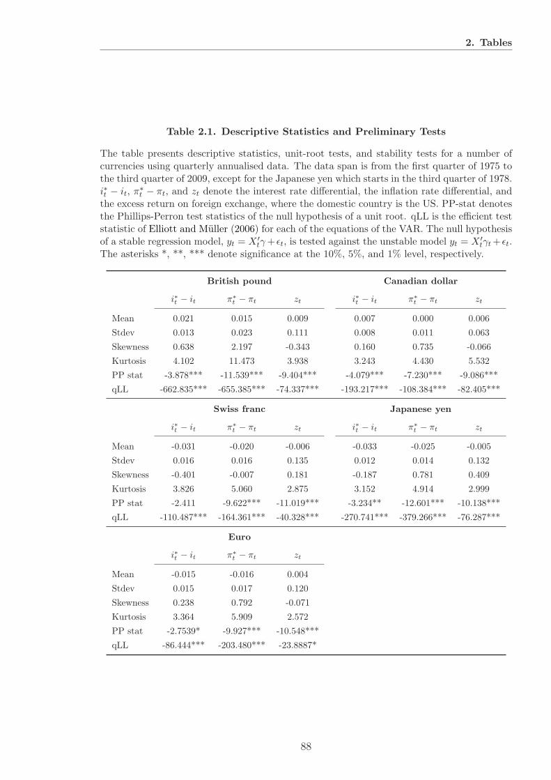
2. Tables
Table 2.1. Descriptive Statistics and Preliminary Tests
The table presents descriptive statistics, unit-root tests, and stability tests for a number ofcurrencies using quarterly annualised data. The data span is from the first quarter of 1975 tothe third quarter of 2009, except for the Japanese yen which starts in the third quarter of 1978.i∗t − it, π
∗t − πt, and zt denote the interest rate differential, the inflation rate differential, and
the excess return on foreign exchange, where the domestic country is the US. PP-stat denotesthe Phillips-Perron test statistics of the null hypothesis of a unit root. qLL is the efficient teststatistic of Elliott and Muller (2006) for each of the equations of the VAR. The null hypothesisof a stable regression model, yt = X ′
tγ+ ǫt, is tested against the unstable model yt = X ′tγt+ ǫt.
The asterisks *, **, *** denote significance at the 10%, 5%, and 1% level, respectively.
British pound Canadian dollar
i∗t − it π∗t − πt zt i∗t − it π∗
t − πt zt
Mean 0.021 0.015 0.009 0.007 0.000 0.006
Stdev 0.013 0.023 0.111 0.008 0.011 0.063
Skewness 0.638 2.197 -0.343 0.160 0.735 -0.066
Kurtosis 4.102 11.473 3.938 3.243 4.430 5.532
PP stat -3.878*** -11.539*** -9.404*** -4.079*** -7.230*** -9.086***
qLL -662.835*** -655.385*** -74.337*** -193.217*** -108.384*** -82.405***
Swiss franc Japanese yen
i∗t − it π∗t − πt zt i∗t − it π∗
t − πt zt
Mean -0.031 -0.020 -0.006 -0.033 -0.025 -0.005
Stdev 0.016 0.016 0.135 0.012 0.014 0.132
Skewness -0.401 -0.007 0.181 -0.187 0.781 0.409
Kurtosis 3.826 5.060 2.875 3.152 4.914 2.999
PP stat -2.411 -9.622*** -11.019*** -3.234** -12.601*** -10.138***
qLL -110.487*** -164.361*** -40.328*** -270.741*** -379.266*** -76.287***
Euro
i∗t − it π∗t − πt zt
Mean -0.015 -0.016 0.004
Stdev 0.015 0.017 0.120
Skewness 0.238 0.792 -0.071
Kurtosis 3.364 5.909 2.572
PP stat -2.7539* -9.927*** -10.548***
qLL -86.444*** -203.480*** -23.8887*
88

2. Figures
1985 1990 1995 2000 2005
0.1
0.2
0.3
0.4
0.5
GBP, interest rate differential
1985 1990 1995 2000 2005
0.6
0.8
1
1.2
1.4
1.6
GBP, inflation differential
1985 1990 1995 2000 2005
10
15
20
25
GBP, excess return
Figure 2.1. Standard deviations for GBP
Each chart displays the standard deviation of the innovation in the corresponding VAR equa-tion. The standard deviation is computed as square root of the corresponding diagonal elementof Ωt.
89

2. Figures
1986 1991 1996 2001 2006
0.1
0.15
0.2
0.25
0.3
0.35
EUR, interest rate differential
1986 1991 1996 2001 2006
0.5
1
1.5
EUR, inflation differential
1986 1991 1996 2001 2006
10
15
20
25
30
EUR, excess return
Figure 2.2. Standard deviations for EUR
Each chart displays the standard deviation of the innovation in the corresponding VAR equa-tion. The standard deviation is computed as square root of the corresponding diagonal elementof Ωt.
90

2. Figures
1985 1990 1995 2000 2005
0.1
0.15
0.2
0.25
0.3
CAD, interest rate differential
1985 1990 1995 2000 2005
0.4
0.6
0.8
1
CAD, inflation differential
1985 1990 1995 2000 2005
5
10
15
20
25CAD, excess return
Figure 2.3. Standard deviations for CAD
Each chart displays the standard deviation of the innovation in the corresponding VAR equa-tion. The standard deviation is computed as square root of the corresponding diagonal elementof Ωt.
91

2. Figures
1985 1990 1995 2000 2005
0.1
0.2
0.3
0.4
0.5
0.6
CHF, interest rate differential
1985 1990 1995 2000 2005
0.4
0.6
0.8
1
1.2
1.4CHF, inflation differential
1985 1990 1995 2000 2005
15
20
25
30
CHF, excess return
Figure 2.4. Standard deviations for CHF
Each chart displays the standard deviation of the innovation in the corresponding VAR equa-tion. The standard deviation is computed as square root of the corresponding diagonal elementof Ωt.
92
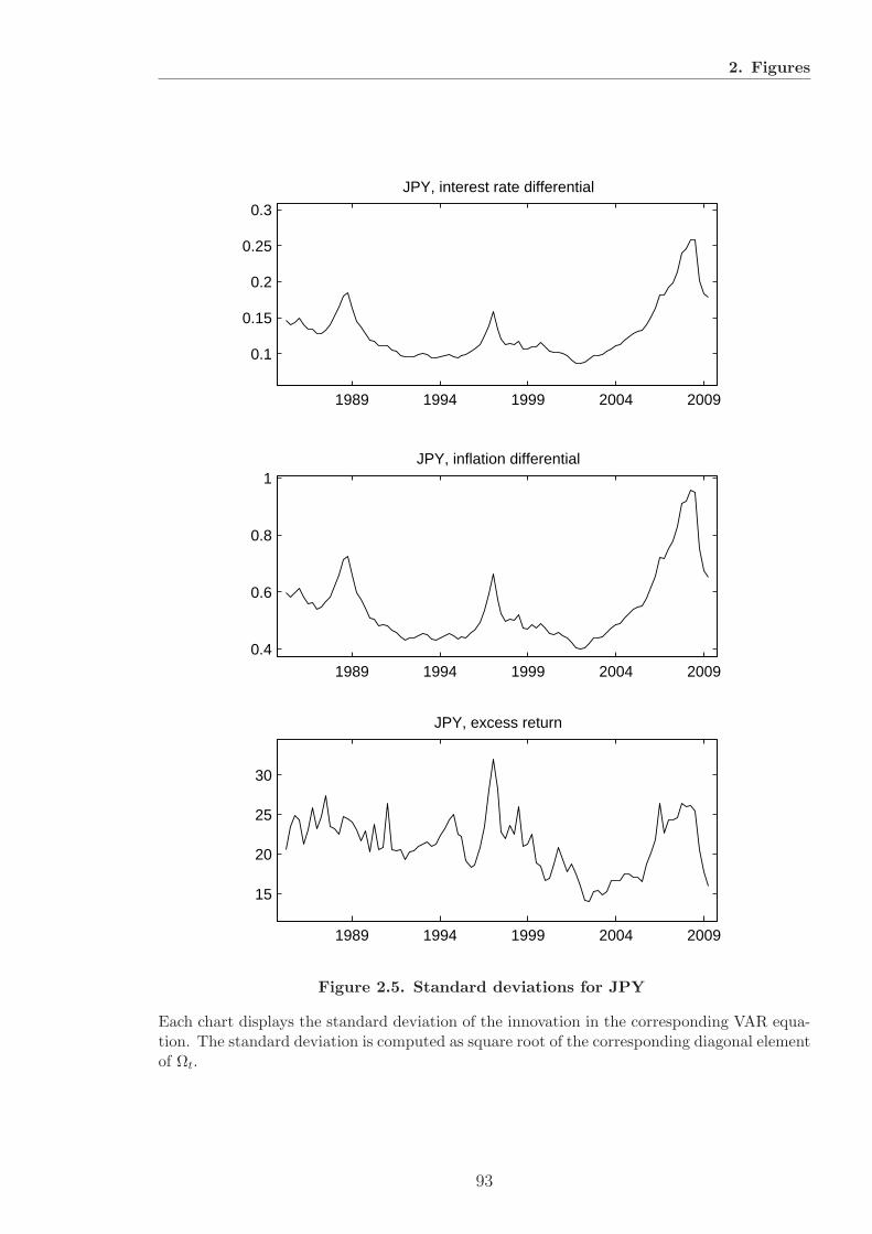
2. Figures
1989 1994 1999 2004 2009
0.1
0.15
0.2
0.25
0.3
JPY, interest rate differential
1989 1994 1999 2004 2009
0.4
0.6
0.8
1JPY, inflation differential
1989 1994 1999 2004 2009
15
20
25
30
JPY, excess return
Figure 2.5. Standard deviations for JPY
Each chart displays the standard deviation of the innovation in the corresponding VAR equa-tion. The standard deviation is computed as square root of the corresponding diagonal elementof Ωt.
93

2. Figures
3 6 9 12 15 18−5
0
5
10
15
20
25Cumulative excess return, 1985 Q4
3 6 9 12 15 18−5
0
5
10
15
20Cumulative excess return, 1995 Q4
3 6 9 12 15 18−10
−5
0
5
10
15
20Cumulative excess return, 2005 Q4
3 6 9 12 15 18−10
−5
0
5
10
15
20Cumulative excess return, 2008 Q4
Figure 2.6. GBP Impulse responses
The charts display the estimated accumulated time-varying impulse responses of the currencyexcess return to a 1% shock to the interest rate differential (i∗ − i). The bold line indicatesthe posterior median, whereas the dashed lines indicate the 16-th and 84-th percentiles. Thedashed horizontal line in each graph is the estimated cumulative excess return implied by UIP(Equation 2.4), reflecting the present value of all the future real interest rate differentials aspredicted by the VAR.
94
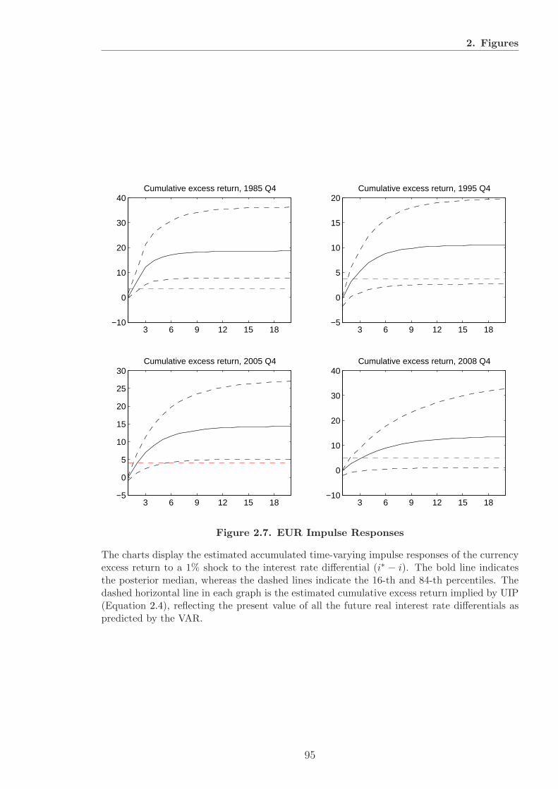
2. Figures
3 6 9 12 15 18−10
0
10
20
30
40Cumulative excess return, 1985 Q4
3 6 9 12 15 18−5
0
5
10
15
20Cumulative excess return, 1995 Q4
3 6 9 12 15 18−5
0
5
10
15
20
25
30Cumulative excess return, 2005 Q4
3 6 9 12 15 18−10
0
10
20
30
40Cumulative excess return, 2008 Q4
Figure 2.7. EUR Impulse Responses
The charts display the estimated accumulated time-varying impulse responses of the currencyexcess return to a 1% shock to the interest rate differential (i∗ − i). The bold line indicatesthe posterior median, whereas the dashed lines indicate the 16-th and 84-th percentiles. Thedashed horizontal line in each graph is the estimated cumulative excess return implied by UIP(Equation 2.4), reflecting the present value of all the future real interest rate differentials aspredicted by the VAR.
95

2. Figures
3 6 9 12 15 18−2
0
2
4
6
8
10
12Cumulative excess return, 1985 Q4
3 6 9 12 15 18−2
0
2
4
6
8
10
12Cumulative excess return, 1995 Q4
3 6 9 12 15 18−5
0
5
10
15Cumulative excess return, 2005 Q4
3 6 9 12 15 18−5
0
5
10
15Cumulative excess return, 2008 Q4
Figure 2.8. CAD Impulse Responses
The charts display the estimated accumulated time-varying impulse responses of the currencyexcess return to a 1% shock to the interest rate differential (i∗ − i). The bold line indicatesthe posterior median, whereas the dashed lines indicate the 16-th and 84-th percentiles. Thedashed horizontal line in each graph is the estimated cumulative excess return implied by UIP(Equation 2.4), reflecting the present value of all the future real interest rate differentials aspredicted by the VAR.
96

2. Figures
3 6 9 12 15 18−10
0
10
20
30
40Cumulative excess return, 1985 Q4
3 6 9 12 15 18−5
0
5
10
15
20
25
30Cumulative excess return, 1995 Q4
3 6 9 12 15 18−10
0
10
20
30
40Cumulative excess return, 2005 Q4
3 6 9 12 15 18−10
0
10
20
30
40
50Cumulative excess return, 2008 Q4
Figure 2.9. CHF Impulse Responses
The charts display the estimated accumulated time-varying impulse responses of the currencyexcess return to a 1% shock to the interest rate differential (i∗ − i). The bold line indicatesthe posterior median, whereas the dashed lines indicate the 16-th and 84-th percentiles. Thedashed horizontal line in each graph is the estimated cumulative excess return implied by UIP(Equation 2.4), reflecting the present value of all the future real interest rate differentials aspredicted by the VAR.
97

2. Figures
3 6 9 12 15 18−10
0
10
20
30
40
50Cumulative excess return, 1985 Q4
3 6 9 12 15 18−10
0
10
20
30
40Cumulative excess return, 1995 Q4
3 6 9 12 15 18−10
0
10
20
30
40Cumulative excess return, 2005 Q4
3 6 9 12 15 18−10
0
10
20
30
40
50Cumulative excess return, 2008 Q4
Figure 2.10. JPY Impulse Responses
The charts display the estimated accumulated time-varying impulse responses of the currencyexcess return to a 1% shock to the interest rate differential (i∗ − i). The bold line indicatesthe posterior median, whereas the dashed lines indicate the 16-th and 84-th percentiles. Thedashed horizontal line in each graph is the estimated cumulative excess return implied by UIP(Equation 2.4), reflecting the present value of all the future real interest rate differentials aspredicted by the VAR.
98

2. Figures
1980 1985 1990 1995 2000 2005 2010−10
−5
0
5Conditional UIP deviations, different horizons
Simultaneous4 qtrs8 qtrs20 qtrs
Figure 2.11. Conditional UIP deviations, GBP
The four lines represent the posterior medians of the simultaneous conditional UIP deviations,and the posterior medians of the conditional UIP deviations after 4, 12 and 20 quarters.A positive conditional UIP deviation indicates that the exchange rate undershoots the levelimplied by fundamentals, while a negative conditional deviation indicates overshooting.
99

2. Figures
1980 1985 1990 1995 2000 2005 2010−20
−15
−10
−5
0
5
10Conditional UIP deviations, different horizons
Simultaneous4 qtrs8 qtrs20 qtrs
Figure 2.12. Conditional UIP deviations, EUR
The four lines represent the posterior medians of the simultaneous conditional UIP deviations,and the posterior medians of the conditional UIP deviations after 4, 12 and 20 quarters.A positive conditional UIP deviation indicates that the exchange rate undershoots the levelimplied by fundamentals, while a negative conditional deviation indicates overshooting.
100

2. Figures
1980 1985 1990 1995 2000 2005 2010−6
−5
−4
−3
−2
−1
0
1
2
3
4Conditional UIP deviations, different horizons
Simultaneous4 qtrs8 qtrs20 qtrs
Figure 2.13. Conditional UIP deviations, CAD
The four lines represent the posterior medians of the simultaneous conditional UIP deviations,and the posterior medians of the conditional UIP deviations after 4, 12 and 20 quarters.A positive conditional UIP deviation indicates that the exchange rate undershoots the levelimplied by fundamentals, while a negative conditional deviation indicates overshooting.
101
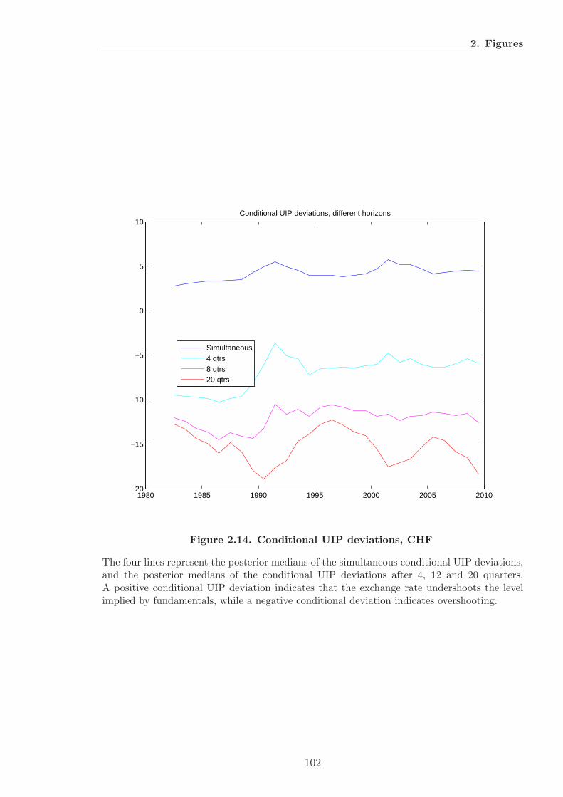
2. Figures
1980 1985 1990 1995 2000 2005 2010−20
−15
−10
−5
0
5
10Conditional UIP deviations, different horizons
Simultaneous4 qtrs8 qtrs20 qtrs
Figure 2.14. Conditional UIP deviations, CHF
The four lines represent the posterior medians of the simultaneous conditional UIP deviations,and the posterior medians of the conditional UIP deviations after 4, 12 and 20 quarters.A positive conditional UIP deviation indicates that the exchange rate undershoots the levelimplied by fundamentals, while a negative conditional deviation indicates overshooting.
102

2. Figures
1985 1990 1995 2000 2005 2010−20
−15
−10
−5
0
5Conditional UIP deviations, different horizons
Simultaneous4 qtrs8 qtrs20 qtrs
Figure 2.15. Conditional UIP deviations, JPY
The four lines represent the posterior medians of the simultaneous conditional UIP deviations,and the posterior medians of the conditional UIP deviations after 4, 12 and 20 quarters.A positive conditional UIP deviation indicates that the exchange rate undershoots the levelimplied by fundamentals, while a negative conditional deviation indicates overshooting.
103
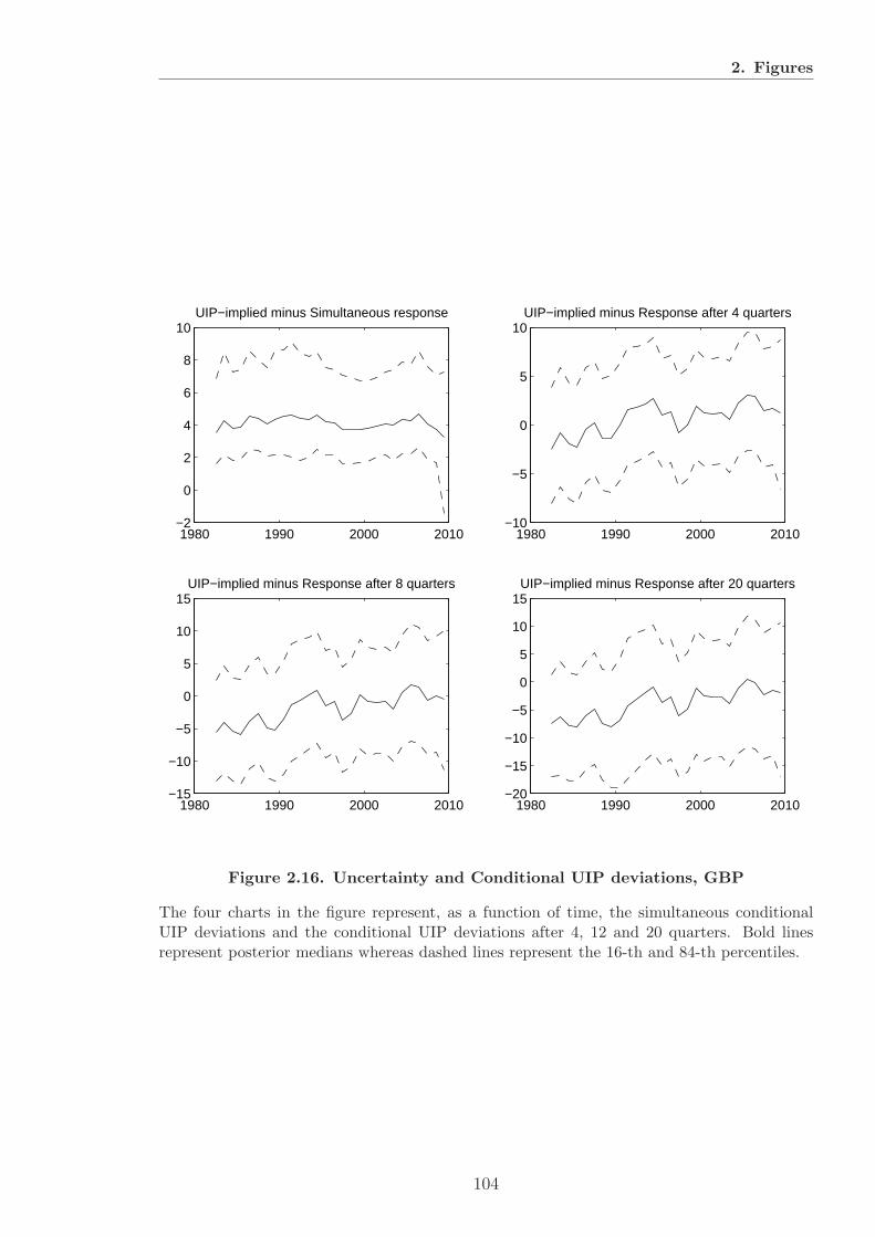
2. Figures
1980 1990 2000 2010−2
0
2
4
6
8
10UIP−implied minus Simultaneous response
1980 1990 2000 2010−10
−5
0
5
10UIP−implied minus Response after 4 quarters
1980 1990 2000 2010−15
−10
−5
0
5
10
15UIP−implied minus Response after 8 quarters
1980 1990 2000 2010−20
−15
−10
−5
0
5
10
15UIP−implied minus Response after 20 quarters
Figure 2.16. Uncertainty and Conditional UIP deviations, GBP
The four charts in the figure represent, as a function of time, the simultaneous conditionalUIP deviations and the conditional UIP deviations after 4, 12 and 20 quarters. Bold linesrepresent posterior medians whereas dashed lines represent the 16-th and 84-th percentiles.
104

2. Figures
1980 1990 2000 20100
5
10
15
20UIP−implied minus Simultaneous response
1980 1990 2000 2010−30
−20
−10
0
10
20UIP−implied minus Response after 4 quarters
1980 1990 2000 2010−40
−30
−20
−10
0
10UIP−implied minus Response after 8 quarters
1980 1990 2000 2010−40
−30
−20
−10
0
10UIP−implied minus Response after 20 quarters
Figure 2.17. Uncertainty and Conditional UIP deviations, EUR
The four charts in the figure represent, as a function of time, the simultaneous conditionalUIP deviations and the conditional UIP deviations after 4, 12 and 20 quarters. Bold linesrepresent posterior medians whereas dashed lines represent the 16-th and 84-th percentiles.
105

2. Figures
1980 1990 2000 2010−4
−2
0
2
4
6
8
10UIP−implied minus Simultaneous response
1980 1990 2000 2010−10
−5
0
5
10UIP−implied minus Response after 4 quarters
1980 1990 2000 2010−10
−5
0
5
10UIP−implied minus Response after 8 quarters
1980 1990 2000 2010−15
−10
−5
0
5
10UIP−implied minus Response after 20 quarters
Figure 2.18. Uncertainty and Conditional UIP deviations, CAD
The four charts in the figure represent, as a function of time, the simultaneous conditionalUIP deviations and the conditional UIP deviations after 4, 12 and 20 quarters. Bold linesrepresent posterior medians whereas dashed lines represent the 16-th and 84-th percentiles.
106

2. Figures
1980 1990 2000 20100
2
4
6
8
10
12UIP−implied minus Simultaneous response
1980 1990 2000 2010−20
−15
−10
−5
0
5UIP−implied minus Response after 4 quarters
1980 1990 2000 2010−25
−20
−15
−10
−5
0
5UIP−implied minus Response after 8 quarters
1980 1990 2000 2010−40
−30
−20
−10
0UIP−implied minus Response after 20 quarters
Figure 2.19. Uncertainty and Conditional UIP deviations, CHF
The four charts in the figure represent, as a function of time, the simultaneous conditionalUIP deviations and the conditional UIP deviations after 4, 12 and 20 quarters. Bold linesrepresent posterior medians whereas dashed lines represent the 16-th and 84-th percentiles.
107

2. Figures
1980 1990 2000 20100
2
4
6
8
10
12UIP−implied minus Simultaneous response
1980 1990 2000 2010−15
−10
−5
0
5UIP−implied minus Response after 4 quarters
1980 1990 2000 2010−25
−20
−15
−10
−5
0
5UIP−implied minus Response after 8 quarters
1980 1990 2000 2010−40
−30
−20
−10
0UIP−implied minus Response after 20 quarters
Figure 2.20. Uncertainty and Conditional UIP deviations, JPY
The four charts in the figure represent, as a function of time, the simultaneous conditionalUIP deviations and the conditional UIP deviations after 4, 12 and 20 quarters. Bold linesrepresent posterior medians whereas dashed lines represent the 16-th and 84-th percentiles.
108
Chapter 3
Currency fair value models
3.1 Introduction
What is the fair value of a currency? Policymakers and international investors have
always been asking this question, and economists have been trying to find answers,
proposing many different methodologies to estimate fair value. Simple measures have
ranged from relative national price indices (Cassel, 1918) to relative hamburger prices
(The Economist, 6 September 1986). More elaborate models take into consideration
economic factors, ranging from productivity differentials (Harrod, 1933; Balassa, 1964;
Samuelson, 1964) to men-women sex ratios (Du and Wei, 2011). In this chapter we pro-
vide a comprehensive review of models that are used by policymakers and international
investors in order to assess exchange rate misalignments from their fair value.
Policymakers need to assess the possible misalignment of currencies for a number of
reasons. Exchange rates play a crucial role in a country’s external adjustment process,
particularly as economies become more and more integrated. At the time of writing,
advanced economies have faced some degree of exchange rate realignment since the
onset of the recent global financial crisis, whereas this realignment has been limited for
emerging market economies, creating tensions and constituting a threat to the global
recovery (IMF, 2011, Chapter 1). More generally, substantial misalignments can have
severe consequences, as exchange rates may abruptly adjust when the misalignment
becomes unsustainable, leading to currency crises generally associated with large output
109

3.1. Introduction
contractions, especially in emerging markets (Dornbusch et al., 1995; Gupta et al., 2007;
Gourinchas and Obstfeld, 2011). In a theory paper, Engel (2011) shows that currency
misalignments are inefficient, lower world welfare, and should be targeted by monetary
policymakers in a model in which firms price to market and prices are sticky.
In Transition Economies, especially for countries of Central and Eastern Europe, the
apparent trend appreciation of the real exchange rates of some of these countries raised
the question of whether this appreciation reflected an adjustment to fair value or not
(Egert et al., 2006). De Broeck and Sløk (2006) show how real exchange rates were
generally misaligned at the onset of the transition and how most of the misalignment
was eliminated over a relatively short period. In developing countries an overvalued
currency can represent a major obstacle for a successful development strategy (Johnson
et al., 2007).
For currency unions it is critically important to get a sense of fair value to assess the
subsequent adjustment needs via relative inflation rates. And for heavily managed or
pegged exchange rates, a fair value estimate may help establish policy targets. However,
because exchange rates are a policy tool for the authorities of a country, and because
there is the potential to use the currencies value to gain an advantage over another
country, the political debate of fair value has always been contentious. The most recent
example are the attempts to determine fair value for the Chinese currency (e.g., Cline
and Williamson, 2008, 2011).
Investors and other agents engaging in international transactions, including trade,
are interested in estimating the fair value of the currency as an input in hedging and
investment strategies. For example, fair value models are useful to assess crash risks in
popular currency speculation strategies. Exchange rates may be pushed away from fun-
damentals by carry trades, occasionally reverting back abruptly and leading to sudden
losses (Brunnermeier et al., 2009; Plantin and Shin, 2011).
A number of investment strategies try to exploit long-run reversion to fair value
by taking a long position in undervalued currencies and a short position in overvalued
currencies. They typically provide lower risk-adjusted returns than carry strategies,
110
3.1. Introduction
but they seem to be less prone to crash risk (Jorda and Taylor, 2009; Nozaki, 2010).
Major financial institutions recently introduced fully investable and tradable indices
that track the performance of such strategies, such as Goldman Sachs FX Valuation
Current (Goldman Sachs, 2009) and Deutsche Bank Valuation Index (Deutsche Bank,
2007).
Strategic Foreign Direct Investments (FDI) decisions with very long investment ho-
rizons may be affected by currency values. Variable real exchange rates may influence
the location of production facilities chosen by multinationals (see e.g. Goldberg and
Kolstad, 1995) and a fair value estimate may be useful as a long-term forecast.
Given the diverse use of currency fair value models highlighted above, it is important
to understand which models are more suitable for a given context. In this chapter we
analyse this issue in detail by surveying and critically assessing a number of fair value
models proposed in the literature.1 We intentionally avoid an extensive discussion of
purchasing power parity (PPP), as this literature is covered in detail in many surveys:
see for example Sarno and Taylor (2003, Chapter 3) and Taylor and Taylor (2004).
We start by providing a short history of fair value models in the literature in the
next section. In Section 3.3, we discuss the basic characteristics of fair value models
with a particular focus on how implicit or explicit design choices typically affect the
results, the robustness and the general usability of these models.
Section 3.4 provides an exposition of a number of fair value and equilibrium exchange
rate models that are widely used in practice. In particular, we focus on the two main
families of fair value models, namely the behavioural equilibrium exchange rate (BEER)
and the underlying balance (UB) models. As case studies we then discuss in more detail
the IMF framework, as well as Goldman Sachs Dynamic Equilibrium Exchange Rate
(GSDEER) model. In both cases we highlight how the estimates of fair value are af-
fected by some typical implementation choices. We also illustrate a fair value concept
extensively used by financial markets practitioners but not previously formalised in the
academic literature. This model, which we dub Indirect Fair Value (IFV), relies on indi-
1As highlighted below, we focus on the practical implementation of these models. For their theore-tical foundations, see e.g. Chinn (2011).
111

3.2. Currency Fair Value in the Historical Context
rect estimation of fair value of the currency by “removing” the speculative components
that drive exchange rates in the short run.
We argue that there is no explicit answer regarding which model delivers the cor-
rect fair value of a currency, because each model has its own individual strengths and
weaknesses. We illustrate this point by means of examples, focusing on the practical im-
plementation of the models. For instance, we discuss the sensitivity of UB models with
regard to variations in import and export elasticities, and show how the different speci-
fications of productivity can affect the results in “adjusted-PPP” models. Moreover, we
discuss how the treatment of external balance in different models appears responsible
for discrepancies between estimation results. Researchers are therefore left with a wide
range of estimates, and many use a set of models or a combination of these in order to
assess exchange rate misalignments.
3.2 Currency Fair Value in the Historical Context
Modelling the fair value of a currency is a relatively young field of economics with the
bulk of the research published in the last 30 years. However, a “primitive” notion of a
fair currency value has probably been around for as long as currencies exist. Vaughan
(1675) makes the following observations in the context of governments reducing the
precious metal content of their currency:
There are two causes of the raising of Money: [. . . ] But the [. . . ] most
frequent cause hath been, an Art which States have used to rob one another
of their Money, by setting on higher prices upon it; so that some States
being induced, by an unjust device, to draw to themselves the Money of
their Neighbours, and others by a necessity to keep their own.
Vaughan continues with an example going back to ancient times:
But first to shew the Antiquity of the practice of raising of Monies we will
begin with the Romans. The As, which was originally coyned of a pound
112

3.2. Currency Fair Value in the Historical Context
weight, was, during the first Punick War for help of publick necessities,
brought to 2 ounces,[...]
This historic reference is particularly interesting because it links a notion of fairness to
a currency value qualifying the exchange rate as “an unjust device”. In fact, Vaughan
describes currencies, which are overvalued because their precious metal content has been
reduced relative to a previous norm, but unknowingly to the users of the currency. In
the same book, he also discusses the “intrinsical value” of money and describes a way
to “equalize the exchange”, which consists of comparing the precious metal content of
two coins.
A closely related “primitive” example of fair value model is Purchasing Power Parity
(PPP), dating back to the Salamanca School in 16th-century Spain (for a history of PPP,
see Officer, 2011). According to PPP, the fair value of an exchange rate between two
countries is determined by the two countries’ relative price levels (Cassel, 1918). In the
same context, early scholars of exchange rates also noted that the increase in money
supply tends to lead to an increase in the general price level.
All these “primitive” examples of fair value go back to the stylised fact that there
seem to be shared long-run trends between monetary fundamentals and the nominal
exchange rate (Frankel and Rose, 1995). In that respect, the basic monetary model of
the exchange rate can be seen as a modern formalised version of the “primitive” notions,
which have been around for centuries. Accumulated changes in money supply could give
valuable hints regarding the fair value of a currency.
Another important concept of fair value was linked to the balance of payment dyna-
mics and in particular to situations which led to a persistent drain of finite foreign ex-
change reserves. Again this analytical approach has to be seen in the historical context.
Governments and rulers had to respond to dwindling gold reserves and tinkering with
the exchange rates had always been one possible option. The related fair value concept of
foreign exchange reserve stability, or some broadly defined external balance, became vi-
sible in the open economy extensions of the IS-LM framework (see for example Mundell,
1963, or Fleming, 1962). Another example is the underlying balance (UB) approach,
113
3.2. Currency Fair Value in the Historical Context
which focuses on the requirements for achieving internal and external balance simulta-
neously (for an overview see for example Isard, 2007).
Interestingly, the collapse of Bretton Woods followed signs of misalignment on the
basis of most of these early fair value concepts. Starting in the 1950s it became increasin-
gly clear that the supply of US dollar grew substantially faster than the amount of gold
that backed the same currency. Triffin (1960) highlighted the linkages between monetary
policy and unsustainable external imbalances in the context of a reserve currency.
With the advent of flexible exchange rates in the post-Bretton Woods area, the
initial basic assumption was that balance of payment imbalances could no longer persist
on a permanent basis. The exchange rate was now able to freely adjust to fair value
without the explicit input from policymakers. Determining fair value was therefore
less of a policy priority. Indeed, the dollar initially weakened from overvalued Bretton
Woods levels and the US external balance improved. However, it became quickly clear
that nominal and in particular real exchange rates displayed far more volatility than
under the previous fixed regime (Mussa, 1986). Research focus shifted to exchange rate
determination, often using variations of the monetary model. However, the difficulty
of beating the Meese and Rogoff (1983) random walk yardstick not only undermined
the usefulness of these models, it also implicitly suggested that the concept of fair value
may be meaningless under floating exchange rates. A further blow to the concept of fair
value came from the lack of empirical support for the PPP hypothesis in the first years
of floating exchange rates (Frenkel, 1981, Taylor and Taylor, 2004).
The interest in being able to assess the fair value of currency started to re-emerge
from the late 1980s onwards. Three developments supported this trend. First, time
series covering the period of floating exchange became longer, which helped empirical
models to pick up long-run regularities (Mark, 1995). Second, advances in econometrics,
in particular the development of unit-root tests (Dickey and Fuller, 1979), cointegration
analysis (Engle and Granger, 1987) and panel data gradually led to the realisation
that the earlier rejection of the PPP hypothesis may have been pre-emptive. Third,
the US dollar appreciated rapidly in response to very tight monetary policy under the
114

3.2. Currency Fair Value in the Historical Context
Fed chairmanship of Paul Volcker, which in turn led to significant and rapid widening
of the US current account deficit. Policymakers quickly realised that exchange rates
misalignment once again started to have a severe impact on the economic situation. As
a result, the focus on the fair value of currencies increased in the run-up to the Plaza
Accord (Funabashi, 1988).
These three developments essentially prepared the ground for a completely new gene-
ration of fair value models, which were no longer focused on the precious metal content
of money. The last 20–30 years have seen a proliferation of models and tools—some
grounded on economic theory, others of largely statistical nature. With every specifica-
tion implicit choices are being made, which affect the usefulness for the potential user
of the fair value model. And not all potential issues can be overcome. It is therefore
increasingly becoming common practice to use a combination of fair value models, kno-
wing that each of them may have potential strengths and shortcomings in the context
of individual user’s needs (IEO, 2007).
Among the large number of different approaches, there are two dominating fami-
lies of currency fair values, which are widely used today. The first group are so-called
Behavioural Equilibrium Exchange Rate (BEER) models, which typically attempt to
directly estimate the reduced-form long-run relationships between a set of macroecono-
mic variables and the exchange rate. These models typically require long datasets, use
cointegration analysis and rely on the assumed stability of the underlying equilibrium
relations.
The second family of models retains as core feature the idea that external imbalances
are unsustainable in the long run and have to be seen as variations of the old Underlying
Balance (UB) models adopted for flexible exchange rates. The underlying approach of
these UB models can be summarised in a hypothetical question from a policymaker:
“By how much do I have to move the currency to bring my current account back to a
sustainable level assuming full employment?” Variants of UB models are widely used
by economists advising policymakers and were initially developed by the International
Monetary Fund (IMF) and by the Washington DC-based Peterson Institute of Inter-
115

3.3. Characteristics of Fair Value Models
national Economics (Williamson, 1983). Modern UB models typically derive a current
account target and then use trade elasticities to determine the necessary exchange rate
movement to reach that target.
3.3 Characteristics of Fair Value Models
In this section, we will try to highlight the most important generic characteristics of
different fair value models. Given the applied nature of this branch of economic research
it is useful to be explicit on how these chosen characteristics potentially affect the model
results. In later sections, it will also be easier to make reference to these characteristics
when discussing specific fair value models.
3.3.1 Horizon/Frequency
A major dimension of fair value models is the time horizon of the analysis. A number
of authors have implicitly or explicitly assumed that the observed exchange rate will
converge to different fair values depending on the horizon. The speed of convergence is
also one of the most important features for the applied use of fair value models.
Driver and Westaway (2004), in a framework similar to that of Clark and MacDo-
nald (1998), start from the following reduced-form relation which relates the observed
exchange rate to a number of explanatory variables:
et = β′Zt + θ′Tt + ǫt, (3.1)
where et is the exchange rate, broadly defined,2 Zt is a vector of medium and long-term
economic fundamentals, Tt is a vector of short-term, transitory factors, ǫt is a residual
term, and β and θ are coefficient vectors.
Driver and Westaway define short-run equilibrium as the exchange rate which would
pertain when its fundamentals are at their current (e.g. observed) values at time t,
2For illustrative purposes, we do not specify here if the exchange rate is defined in nominal or realterms, bilateral or effective.
116

3.3. Characteristics of Fair Value Models
abstracting from the influence of asset market bubbles. In a notation similar to Clark
and MacDonald, they define the short-term equilibrium as
et = β′Zt + θ′Tt. (3.2)
This is what Williamson (1983) and Clark and MacDonald (1998) call the current equi-
librium exchange rate. The half-life of misalignments in applied models containing ob-
served values of cyclical variables would likely be measured in weeks or months.
Industry practitioners often attempt to use direct measures of speculative positio-
ning to decompose the exchange rate into an “observed” speculative component and an
unobserved fair value. Fair value models of this kind tend to display half-lives that can
typically be measured in days or weeks, and therefore can be considered as an attempt
to identify the fair value of a currency for the very short term. We will discuss in more
detail these models in Section 3.4.5.
The medium-run fair value3 can be described by the following reduced-form equation,
et = β′Zt, (3.3)
where the hat indicates that the variables abstract from cyclical components. In most
empirical applications, this often translates in (i) excluding fundamentals which are
typically thought to characterize only cyclical deviations from the equilibrium level4
and in (ii) the fundamentals being set at their trend values. Though consistent with a
flow equilibrium, the medium-run fair value may still allow adjusting towards a long-run,
stock equilibrium. For example the net foreign asset position may still be changing.
Using the Driver and Westaway (2004) notation again, a long-term equilibrium is
3Driver and Westaway (2004) define the medium-run equilibrium as the exchange rate which iscompatible with the economy being at internal and external balance. For the concept of internal andexternal balance, see Sections 3.4.2 and 3.5.1.
4For example by excluding interest rate differentials from the analysis, as exchange rates tend toinherit the cyclical properties of interest rate differentials (see e.g. Lustig et al. 2010).
117

3.3. Characteristics of Fair Value Models
defined as the point where a stock equilibrium is achieved for all agents in the economy:
et = β′Zt, (3.4)
where the overbar denotes the long-run values of variables. Long-run fair values mo-
dels are therefore mostly used when studying structural sources of misalignment. For
example, a reserve currency will tend to be overvalued in the long run as its economy
will tend to run current account deficits, and therefore a depreciation will be needed
for restoring the long-run equilibrium. Other examples of structural misalignment are
commodity-exporting countries with growing sovereign wealth funds, or central banks
following a policy of deliberate undervaluation and systematic intervention.
Fair value estimates will therefore reflect the choice in the selection of fundamentals.
Particularly, models which try to directly estimate reduced form equations such as (3.2)
to (3.4) will be particularly affected: as they use the fitted value as an estimate of
fair value, they tend to inherit the statistical properties of the explanatory variables
used. This fact will in turn affect the estimated size and duration of exchange rate
misalignments.
3.3.2 Direct econometric estimation versus “methods of calcu-
lation”
One may attempt to compute currency’s fair value by directly estimating a reduced form
equation relating the level of the exchange rate to a set of fundamental variables. This
reduced form equation takes generally the form of a long-run cointegrating relationship,
whose short-run dynamics may be estimated using an Error Correction Model (ECM).
The BEER models discussed in Section 3.4 belong to this family.
These models are useful in order to characterise the time variation properties of
exchange rates, and therefore may provide some forecasting power. However, as these
models rely on the assumption of stable long-run relations, their estimation may be
plagued by the limited availability and poor quality of historical data. Especially in the
118

3.3. Characteristics of Fair Value Models
case of emerging markets and less developed economies, the presence of small samples,
systematically managed or pegged exchange rates, and data from unreliable sources may
severely bias the estimated coefficients.
Another approach, e.g. the one followed by the fundamental equilibrium exchange
rate (FEER) model (see Section 3.4.2) and by the IMF’s External Sustainability ap-
proach (see Section 3.5.3), is to start from a simple macroeconomic relationship bet-
ween the exchange rate and an economic policy objective (such as target capital flows
or current accounts). Then, calculate the implied exchange rate change (from prevailing
levels) that would be required in order to reach that objective. These models can be so
considered as a “method of calculation” (Wren-Lewis, 1992), since they require no (or
minimal) econometric estimation.
Among the advantages of this latter family of models are the fact that their simple
structure makes them less reliant on data availability issues, and that they take policy
objectives explicitly into consideration. In general, they also provide a useful reference
point that can be compared to exchange rate assessments obtained using more com-
plicated econometric models. On the other hand, they often rely on relatively strong
assumptions, making them less robust in empirical applications in which these assump-
tions are likely to be violated (see e.g. Section 3.5.4).
3.3.3 Treatment of External Imbalances
External imbalances are an implicit or explicit part of most fair value models and often
are the very core of the model. However, defining an external imbalance is in practice
more difficult than one may expect and there are a number of issues that have to be
considered when using external imbalances in fair value models. We discuss here some
of these issues:
• Defining which part of an external imbalance is of cyclical nature and which part is
of structural nature is not trivial. Policy choices can drive structural imbalances:
for example, the choice of pegged or managed exchange rate regimes, the exis-
tence of sovereign wealth funds or persistent fiscal policy differentials. Structural
119

3.3. Characteristics of Fair Value Models
imbalances can also be driven by the choice of reserve currency, or depend on the
natural endowment of commodities. These factors have implications for assessing
both the observed and the equilibrium levels of the current account, and therefore
have to be recognized explicitly when modelling currency fair values. Sub-optimal
modeling choices with regards to these issues could for example lead to foreign
exchange policy recommendations that would condemn a country to a state of
permanent Dutch disease as a result of commodity driven current account sur-
pluses. As we discuss in Sections 3.4 and 3.5, these choices are explicitly reflected
in many fair value models, while others simply assume that external imbalances
will correct themselves over time.
• Fair value models based on the idea of sustainable current account positions should
respect the “N-1” global consistency requirement (Faruqee, 1998), given that the
sum of global current account balances should add up to zero.
• Many models use trade elasticities to calculate the necessary exchange rate changes
needed to reach an external balance target. However, as we show in Section
3.5.4, this approach is highly sensitive to errors in the estimation of trade elastici-
ties. Even very small changes in estimated trade elasticities can create substantial
changes in fair value estimates. Moreover, the very idea of using exchange rates to
address external imbalances is based on the assumption that the Marshall-Lerner
condition holds, an assumption that should ideally be tested.
• When using measures of external imbalances in time-series-based fair values, the
estimated coefficients on the external variables often show the “wrong” (i.e., coun-
terintuitive) signs. For example, the estimates may show that the fair value ap-
preciates with growing current account deficits. Obviously, the idea of external
sustainability would suggest the opposite, namely that growing current account
deficits lead to a depreciated fair value estimate. A weaker currency in a fair value
sense would then help reduce the external imbalances. There could be several rea-
sons for this empirical problem. For example the Marshall-Lerner condition may
120

3.3. Characteristics of Fair Value Models
not hold as already discussed above. More likely, however, is a contamination
of the estimates by cyclical effects. Most models of exchange rate determination
would suggest that a small open economy facing a positive domestic demand shock
will likely experience an appreciating currency at the same time as a deterioration
of the current account balance. Fair value models with wrong signs may therefore
simply pick up these cyclical forces. Explicitly correcting for these cyclical fac-
tors may be one solution. Alternatively, dropping the external variable is a very
simple solution, which is based on the assumption that over the long run external
imbalances will mean-revert to equilibrium levels.
Therefore, in terms of modelling choices, the treatment of external imbalances tends
to have a notable impact on fair value estimates and careful consideration of the explicit
or implicit choices is important. As will be discussed more in subsequent sections,
estimates of fair value based on variants of the Underlying Balance (UB) model tend to
be far more sensitive to the extent of current account imbalances than those from most
BEER or adjusted-PPP models.
3.3.4 Real versus Nominal Exchange Rates
In most cases, it will be reasonably easy to map the results of a nominal fair value model
into real exchange rates and vice versa. But data limitations may play a role. There is a
wide variety of inflation data available but not necessarily comparable across countries.
Moreover, inflation data may be available at weekly, monthly or only quarterly intervals
and hence affect the underlying horizon/frequency of the model. The vast majority of
theory-driven models rely on real exchange rates.
3.3.5 Bilateral versus Effective Exchange Rate
The choice between bilateral and effective (i.e. multilateral) exchange rates is crucial
when assessing exchange rate misalignments empirically. Effective exchange rates have
the advantage that they allow making a fair value assessment for a single currency,
whereas a bilateral fair value calculation always depends on influences by two countries.
121

3.3. Characteristics of Fair Value Models
Bilateral fair value signals are often misinterpreted when the anchor currency itself is
misaligned on a broad basis—an issue frequently encountered in the last few years when
the US dollar has been undervalued according to many fair value models. In that case
assessing multilateral misalignment may be more useful but at the same time it may
suffer more from constraints on data availability, as this approach requires collecting
data from many countries.
Effective exchange rates also depend on the weighting scheme used to calculate the
basket. Many different trade-weighted baskets are used in practice, including some al-
ternative weighting schemes based on capital flows or even volatility. Weighting schemes
with static weights suffer from lack of representativeness after a period of changing trade
patterns in the global economy (see Chinn, 2006).
Bilateral fair value calculations are less demanding on data availability and less
influenced by the choice of weighting scheme.5 In particular for descriptive modelling
approaches, bilateral exchange rates have the conceptual advantage of being actually
observable in the markets.
In general, it is possible to transform bilateral exchange rate fair value estimates into
effective exchange rate estimates, simply by applying the trade weights and calculating
the geographic average. The reverse is also possible. Alberola et al. (1999) suggest a
procedure to extract bilateral misalignments from a vector of effective misalignments.
See also the approach used by Cline (2008).
3.3.6 Time Series versus Cross-Section or Panel
The choice of the estimation procedure is largely an econometric issue, which we will
not discuss here, but its seems worthwhile highlighting an important trade-off when
choosing between a single-equation estimate and a panel with homogeneous coefficients
for all cross-sectional units.
With many countries having different economic structures, it is possible that there
5Clearly, bilateral real exchange rates will still depend on the weighting scheme of the chosen priceindex.
122
3.3. Characteristics of Fair Value Models
are different relations between macro variables and the respective currencies. Imposing
the same coefficients across currencies in a panel may therefore not fully reflect the
country-specific characteristics. One possible solution is to break a panel into more
homogeneous sub-panels and ultimately to estimate fair values for individual currencies.
On the other hand, a panel allows assessing the potential influence on fair value of a
factor that has not been relevant for a currency in the past. For example, the discovery
of a previously unknown natural resource in a country may affect fair value, but it will
be impossible to quantify the impact in a single-equation approach because of the lack
of historical data. On the contrary, a panel estimate allows quantifying the impact if
other currencies in the panel have been affected by a similar discovery in the past.
One possible constraint for using a panel however is data availability. A comparable
dataset for each cross section unit is necessary and may seriously restrict the number
of possible explanatory variables and the size of the dataset. A frequently used panel
cointegration technique is the panel dynamic ordinary least squares (DOLS), see e.g.
Stock and Watson (1993) and Mark and Sul (2003).
3.3.7 Model Maintenance
As highlighted above, one interesting feature of fair value models is that they are often
an important input for policy decisions or investments. This creates special demands
on the timeliness of estimates, data availability, and data quality.
General model maintenance is an important aspect in applied work when more than
a point estimate is needed. The frequency of updates and re-estimation needs to be
determined. Validation procedures may need to be implemented to assess the impact of
data revisions on the fair value estimates. Fitted fair values may change when statistical
agencies change the frequency, base year or calculation of input data. The quality of
estimates may deteriorate as the sample increases over time. Additional cross sections
my be have to be included in a panel as more data becomes available. Cross-sectional
units may vanish as countries enter currency unions. All these events will likely have a
more or less severe impact on misalignment and hence need to be assessed carefully and
123

3.4. Models/Taxonomy
quickly, before policy or investment decisions start to be influenced by issues related to
model maintenance.
It is important not to underestimate this factor as complex models covering a large
number of countries may rely on thousands of data series from diverse sources. A simple
model that relies on a few standard input variables may prove more robust over time
than a state-of-the-art model with excessively complex and time consuming updating
procedures, which may then result in frequent maintenance errors.
This trade-off between complexity and robustness on the implementation side is an
important factor for any institution planning to use a fair value model on a regular
basis.
3.4 Models/Taxonomy
3.4.1 “Adjusted PPP”: Harrod-Balassa-Samuelson and Penn
Effects
Many studies have tried to measure exchange rate misalignment by exploiting the posi-
tive relation between real per capita income and relative prices across countries, that is,
the fact that rich countries tend to have higher price levels than poor countries. This
empirical relation is also known as the “Penn effect” after the Penn World Table of
Summers and Heston (1991), and has been explained usually by appealing to producti-
vity differentials between the tradeable and non-tradeable sectors—the Harrod-Balassa-
Samuelson effect (see e.g. Rogoff, 1996). This effect provides a structural interpretation
of long-run deviations from PPP (hence the “adjusted PPP” terminology used in many
studies) based on real factors that can be exploited for measuring exchange rate misa-
lignments. The exchange rate misalignment can therefore be measured as the residual
of a cross sectional regression such as
qi = a+ b ln(GDPi) + νi, (3.5)
124

3.4. Models/Taxonomy
where q is the log real exchange rate, a and b are coefficients, ν is the residual term, and
GDP is measured in per capita terms, usually relative to the United States and converted
using PPP-based exchange rates. Frankel (2006) uses this kind of regression in order
to evaluate the renminbi misalignment at two different time points, the years 1990
and 2000. De Broeck and Sløk (2006) adopt a similar methodology for measuring the
misalignment of the real exchange rates for a number of transition economies at the onset
of the transition period. Cheung et al. (2007, 2009) extend the cross-sectional approach
of Frankel (2006) by using panel data techniques for a number of specifications, e.g.
allowing for country fixed effects, random effects, and adding different control variables.
Rodrik (2008) builds an index of currency undervaluation by taking the residuals of an
estimated panel regression of real exchange rates on real per capita income allowing for
time fixed effects.
In Section 3.6 we show in a simple example that estimated fair values based on
the Penn effect can be quite sensitive to the exact specification of productivity in the
tradable goods sector.
3.4.2 The Underlying Balance approach
The underlying balance (UB) approach asserts that the fair value of a currency is the
level of the exchange rate which is consistent with a country’s internal and external
balance. Most applications of the underlying balance approach identify internal balance
as a country’s economic activity being at full potential output (i.e. zero output gap).
External balance can be broadly defined as country’s current account position being at
equilibrium or sustainable levels, but different interpretations of what “equilibrium” or
“sustainable” exactly mean have given rise to different implementations of this approach
in the literature. The underlying balance approach has it roots in the pioneering work
of Nurkse (1945), Metzler (1951), Meade (1951), and Swan (1963), in their attempts
to characterize the equilibrium in an open economy. More than most other fair value
models, the UB approach explicitly considers external imbalances to derive fair value
estimates. We discussed the implications of this important choice in section 3.3.3.
125

3.4. Models/Taxonomy
The underlying balance approach starts from the balance of payments identity which
expresses the current account (CA) in terms of either a change in net foreign assets
(∆NFA) or of the excess domestic savings (S) over domestic investment (I), i.e.
CA = ∆NFA = S − I. (3.6)
The equilibrium exchange rate is then found as the level of the exchange rate that closes
the gap between the current account set to prevail in the medium run when countries are
at internal balance—the underlying current account (UCUR)—and some equilibrium or
sustainable value of (S− I) or ∆NFA—the saving-investment/current account “norm”
or “target” net capital flows.
Figure 3.1 provides a summary of the approach. The UCUR line is downward sloping
because an appreciation of the real effective exchange rate (corresponding here to an
increase in its level) tends to be associated with a declining current account, for a
given level of output. The current account norm, instead, is generally assumed to be
independent of the level of the exchange rate, so that the line is vertical. The equilibrium
level of the real effective exchange rate is therefore associated with the intersection of
the two lines, REER∗.
The estimation of the underlying current account and the current account norm are
distinguishing features of the empirical applications of the underlying balance approach.
We will consider down here the two most prominent cases, i.e. the “fundamental equi-
librium exchange rate” in Section 3.4.2 and the IMF Macroeconomic Balance approach
in Section 3.5.1.
The Fundamental Equilibrium Exchange Rate (FEER)
The term “fundamental equilibrium exchange rate” (FEER) is often used as a syno-
nym for the exchange rate which is consistent with internal and external balance, and
therefore falls into the broad category of models which follow the underlying balance
approach discussed above.
However, here we will use the term FEER to indicate more narrowly the model first
126

3.4. Models/Taxonomy
developed by Williamson (1983, 1994), given its major influence in the development
of exchange rate fair value models. Williamson (1983) defines the FEER as the real
effective exchange rate “generating for every country a current-account surplus or deficit
equal to the underlying capital flow over the cycle, given that the country is pursing
internal balance as best it can and not restricting trade for balance of payments reasons”
(Chapter 2, p. 14).
The main distinguishing feature of FEER with respect to other underlying balance
models (especially, the CGER Macroeconomic Balance model discussed in Section 3.5.1)
is the definition of external balance in terms of “underlying” capital flows. The focus
here is on computing the real effective exchange rate which equates the underlying
current account to an equilibrium level of capital flows. This level is derived not through
estimation procedures but mostly by judgmental considerations, and is often assumed
to be a constant proportion of GDP (Williamson and Mahar, 1998). This is why Wren-
Lewis (1992) defines the FEER model as a “method of calculation” (as opposed to an
econometric estimation) of the equilibrium exchange rate.
Highlighting the normative content of the FEER approach, Bayoumi et al. (1994)
name the approach as “desired equilibrium exchange rate” (DEER). The DEER is the-
refore the exchange rate consistent with internal balance and a target current account
explicitly set (or “desired”) by policymakers. In their application, Bayoumi et al. (1994)
calculate the DEER for a number of countries in 1970 in order to analyse the break-up
of the Bretton-Woods system. They use a one-percent target current account surplus, as
this was the approximate stated objective of the US government during the discussions
that led to the Smithsonian Agreement in 1971 (in general, a one-percent target current
account surplus was also widely supported by the IMF for industrial countries in the
1960s, see also Polak, 1995, p. 749).
In a more recent example of judgmental current account targets, Cline and William-
son (2008, 2011) discuss the appropriate set of current account targets for a number of
developed and emerging economies. They start from the “presumption” that external
imbalances should not exceed 3 percent of GDP in the medium run for any country,
127
3.4. Models/Taxonomy
and then refine the current account target based on judgmental considerations for each
country.
By contrast, the CGER MB model discussed below focuses on the behaviour of the
current account balance as implied by its medium-run determinants, and relies on less
ad hoc assumptions (see the Section 3.5 on the CGER models).
As such, the FEER model is generally considered to be a method of assessment of
currency misalignment, rather than a model of exchange rate determination. However,
it implicitly assumes that the actual exchange rate will exhibit a tendency to revert to
its fair value, at least in the medium run.
3.4.3 The Behavioural Equilibrium Exchange Rate Family of
Models
Clark and MacDonald (1998) propose the estimation of a reduced-form equation in
order to explain the behaviour of the real effective exchange rate both in the short and
medium run—what they call the behavioural equilibrium exchange rate (BEER). As is
the case for the FEER model above, the acronym BEER is often used to indicate, by
extension, a whole family of models which follow similar methodologies.
The Standard BEER Model
The BEER model can be used to estimate what Clark and MacDonald (1998) call the
current misalignment and the total misalignment of a currency. The current misalign-
ment is defined as the difference between actual values of the exchange rate and the
estimated level of the fair value given the current values of the fundamentals. The to-
tal misalignment is instead the difference between actual values of the exchange rate
and the estimated level of the fair value given a measure of the sustainable or long-run
fundamentals.
The theoretical basis of the BEER model is the risk-adjusted uncovered interest
parity condition in real terms. By definition, the log excess return on foreign exchange
128

3.4. Models/Taxonomy
is equal to the interest rate differential plus the appreciation rate of the foreign currency
zt+k = i∗t − it + (st+k − st), (3.7)
where st is the natural logarithm of the exchange rate (defined as the domestic price of
foreign currency, so that an increase in st denotes appreciation of the foreign currency),
and it and i∗t are the continuously compounded k-period domestic and foreign riskless
interest rates, respectively. In terms of the log real exchange rate, defined as qt =
st + p∗t − pt, where p∗t and pt are the logs of the foreign and domestic price levels,
Equation (3.7) can be rewritten as
zt+k = r∗t+k − rt+k + qt+k − qt, (3.8)
where rt+k and r∗t+k denote domestic and foreign real interest rates, respectively. In
general, the expected excess return, Etzt+k, will be equal to a time-varying risk premium,
ρt, so that
qt = Et(qt+k) + Et(r∗t+k − rt+k)− ρt. (3.9)
That is, the equilibrium real exchange rate reflects expectations of future real exchange
rates, expectations of future real interest rate differentials, and a time-varying risk
premium.
To make their model empirically tractable, Clark and MacDonald make the further
assumption that the unobservable expectations of the exchange rate are a function of
long-run economic fundamentals, i.e. Et(qt+k) = β′Zt, where Zt denotes the vector
of fundamentals. They identify the latter as the terms of trade, the relative price of
nontraded to traded goods (proxying for Harrod-Balassa-Samuelson effects), and net
foreign assets. Moreover, they proxy the time-varying risk premium ρt with the relative
supply of domestic and foreign debt, arguing that an increase in the relative supply
of outstanding domestic debt relative to foreign debt will increase the domestic risk
premium, thereby requiring a depreciation of the current equilibrium exchange rate (see
e.g. Giorgianni, 1997).
129

3.4. Models/Taxonomy
Empirically, the BEER is generally estimated using the fitted values of a cointe-
gration relationship between the real effective exchange rate and a set of fundamentals
such as those estimated above. For example, Clark and MacDonald (1998) use the Jo-
hansen (1988) method which allows for the existence of multiple cointegrating vectors.
Extensions of the BEER approach are among the most popular fair value models among
policy institutions and in the financial industry. For example, see the IMF equilibrium
real exchange rate (ERER) approach and Goldman Sachs’s GSDEER model discussed
later in this chapter.
A related approach is the so-called capital enhanced equilibrium exchange rate
(CHEER), introduced by Johansen and Juselius (1992) and MacDonald and Marsh
(1997), and later extended by MacDonald and Marsh (2004). The starting point is
the view that nominal exchange rates may be misaligned form their PPP-implied level
because of non-zero interest rates differentials (what MacDonald and Marsh (1997) call
the “Casselian view” of PPP). A cointegration relation is therefore estimated between
nominal exchange rates, domestic and foreign price levels, and domestic and foreign
interest rates. In this approach, the estimated speed of convergence tends to be faster
than the typical PPP adjustment based on univariate models, and the inferred nominal
exchange rate forecasts have some degree of short-term predictive ability when compared
to the random walk benchmark.
The Permanent Equilibrium Exchange Rate (PEER)
Even though the BEER model explicitly recognises the distinction between current and
total misalignment (see above), most of the actual implementations of BEER models
generally focus only on the former. As the current values of fundamentals may de-
part substantially from sustainable or long-run levels, a number of researchers have
been investigating the fair value of the real exchange rate consistent with its long-run
fundamentals.
Huizinga (1987) and Cumby and Huizinga (1990) use respectively univariate and
multivariate Beveridge-Nelson decompositions in order to decompose the real exchange
130
3.4. Models/Taxonomy
rate into the sum of permanent and transitory components. The permanent component
is then considered to be the permanent equilibrium exchange rate.
More recently, the permanent equilibrium exchange rate (PEER) model of Clark
and MacDonald (2004) is a direct extension of the BEER models outlined above. Clark
and MacDonald use the method developed by Gonzalo and Granger (1995) in order
to decompose the fundamentals in permanent and transitory components, where the
former are used to identify the long-run value of the fundamentals necessary to estimate
the total misalignment defined above. The fundamentals are the same as in the BEER
approach, but the terms of trade and the government debts ratio are dropped in the
empirical analysis.
3.4.4 The natural real exchange rate (NATREX)
Stein (1994) defines the natural real exchange (NATREX) as “the exchange rate that
would prevail if speculative and cyclical factors could be removed while unemployment
is at its natural rate” (Stein, 1994, p. 135). As for the FEER model, the NATREX
model is based on the underlying balance approach.
The NATREX model explicitly recognizes different dynamics for medium and long-
run equilibrium exchange rates. Speculative and cyclical factors influence the exchange
rate at the short horizon, whereas at the medium term is dominated by the stock of
capital, the stock of foreign debt, and a number of fundamentals. The long-term equi-
librium exchange rate is determined solely by the fundamentals, as the stock of capital
and foreign debt are assumed to set at their long-run, steady state values. A number
of different fundamentals have been proposed in empirical work, the most important
of which are identified as domestic and foreign productivity, and domestic and private
propensity to save (the so-called “social thrift”), both at home and abroad.
In the empirical implementations, the NATREX is generally estimated similarly to
the BEER, that is, by identifying a cointegrating relation between the real exchange rate
and a number of fundamentals. Some of these fundamentals are not directly observable
and thus must be proxied. For example, Stein (1994) uses real GNP growth rates in
131

3.4. Models/Taxonomy
order to proxy the growth of capital stock at home and abroad. Moreover, the rate of
change of foreign debt is proxied using the current account to GNP ratio, and propensity
to save is proxied by private and public consumption as a ratio of GNP. The ratios are
used in order to abstract from cyclical factors, the same reason for which most of the
variables are taken as twelve-quarter moving averages. For a detailed exposition of the
NATREX approach, see also Stein (2006).
3.4.5 The Indirect Fair Value
In this section, we discuss an indirect approach to modelling fair value, which is fre-
quently used in financial markets. Relatively few macroeconomic assumptions are being
made with regard to the drivers of the fair value. Instead, the approach depends on
the assumption that speculative activity is the principal cause for misaligned exchange
rates. To our knowledge, this Indirect Fair Value (IFV) approach has not been pre-
viously formalised in the academic literature.
Market participants use this kind of model as a way to assess where the exchange
rate would be had speculative activity not pushed it away from a loosely defined fair
value concept. The idea that speculative activity can create these deviations is based on
two assumptions. First, speculative order flow has an impact on exchange rates (Lyons,
2001). Second, one has to assume that speculative order flow is mean reverting over the
medium term. The latter is a corollary of the definition of speculative activity, which is
based on the assumption that speculators will at some stage reverse their position and
realize either a profit or a loss.
Two measures of speculative positioning often employed in this approach are risk
reversals or International Money Market (IMM) positioning (Mogford and Pain, 2006).
The former is defined as the difference between the implied volatility between compa-
rable out-of-the-money call and put options. When the majority of speculative investors
expect appreciation, demand for call options will likely rise relative to the demand for
puts. As a result the relative price, and implied volatility, will increase for the call
options relative to the put options. The second measure is based on the weekly Com-
132
3.4. Models/Taxonomy
mitments of Traders (COT) Report, which contains information about the positioning
size of so-called non-commercial traders on the IMM futures exchange, part of the Chi-
cago Mercantile Exchange (CME).6 The report is restricted to data for the most liquid
exchange rates against the US dollar.
These measures of speculative positioning tend to be stationary and highly correlated
with spot exchange rates (Campa et al., 1998; Mogford and Pain, 2006). Moreover,
indicators of speculative positioning also tend to be strongly autocorrelated (Dunis and
Lequeux, 2001), which implies that periods of speculatively driven misalignments tend
to persist for a certain time, but typically not more than a few months.
Most measures of speculative positioning have a clearly defined neutral point. For
example risk reversals are equal to zero when the implied volatilities of equivalent out-
of-the-money call and put options are identical. A similar argument applies to the net
positions of non-commercial traders on the IMM. In practice, however, indicators of
speculative positioning tend to oscillate around a non-zero mean. Speculative investors
may on average perceive that the appreciation of a currency is more likely than the
depreciation, or vice versa. Moreover, these indicators can display structural breaks, or
trend stationarity.
In practice, these factors tend to affect the choice of sample size. On one hand
the sample has to be large enough to guarantee stationarity and the mean reverting
properties of the indicators of speculative positioning. On the other hand, longer samples
create the risk of having to deal with trends or structural breaks in the positioning
variable. Practitioners tend to look at daily or weekly data with sample sizes between 6
months and 3 years, which emphasizes the more trading-oriented concept of fair value
underlying this approach. This approach also highlights that the statistical properties
of the input variables play a far bigger role than in most other concepts of fair value.
More formally, we can express the relation between the level of the exchange rate
6See www.cftc.gov/marketreports/commitmentsoftraders/index.htm for details on the COTreports.
133
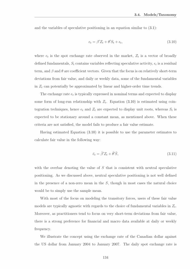
3.4. Models/Taxonomy
and the variables of speculative positioning in an equation similar to (3.1):
et = β′Zt + θ′St + ǫt, (3.10)
where et is the spot exchange rate observed in the market, Zt is a vector of broadly
defined fundamentals, St contains variables reflecting speculative activity, ǫt is a residual
term, and β and θ are coefficient vectors. Given that the focus is on relatively short-term
deviations from fair value, and daily or weekly data, some of the fundamental variables
in Zt can potentially be approximated by linear and higher-order time trends.
The exchange rate et is typically expressed in nominal terms and expected to display
some form of long-run relationship with Zt. Equation (3.10) is estimated using coin-
tegration techniques, hence et and Zt are expected to display unit roots, whereas St is
expected to be stationary around a constant mean, as mentioned above. When these
criteria are not satisfied, the model fails to produce a fair value estimate.
Having estimated Equation (3.10) it is possible to use the parameter estimates to
calculate fair value in the following way:
et = β′Zt + θ′S, (3.11)
with the overbar denoting the value of S that is consistent with neutral speculative
positioning. As we discussed above, neutral speculative positioning is not well defined
in the presence of a non-zero mean in the S, though in most cases the natural choice
would be to simply use the sample mean.
With most of the focus on modeling the transitory forces, users of these fair value
models are typically agnostic with regards to the choice of fundamental variables in Zt.
Moreover, as practitioners tend to focus on very short-term deviations from fair value,
there is a strong preference for financial and macro data available at daily or weekly
frequency.
We illustrate the concept using the exchange rate of the Canadian dollar against
the US dollar from January 2004 to January 2007. The daily spot exchange rate is
134

3.5. IMF CGER - Consultative Group on Exchange Rate Issues
regressed on the difference between US and Canadian 2-year swap rates, as well as
linear, quadratic, and cubic time trends. We use 3-month 25-delta risk reversals as a
measure of speculative positioning in the regression. We conducted several unit-root
tests to confirm that the exchange rate and interest rate differential likely display a unit
root over the sample, while risk reversals are likely stationary. Indeed, Figure 3.2 shows
that risk reversals behave as a stationary time series with a sample mean which is very
close but not equal to zero.
Figure 3.3 illustrates the results. The black line represents the observed daily ex-
change rate between the US and Canadian dollars. The light grey line displays the fitted
value of the regression using the observed values of all right hand variables. Finally, the
dark grey line represents the IFV, which describes where the exchange rate would have
been without the influence of speculative activity. This fair value is computed using
Equation (3.11), i.e. as the fitted exchange rate but using the sample mean of the risk
reversals instead of the observed values.
As Figure 3.3 shows, misalignment from the IFV of up to ten percent occurred in
the sample considered. Moreover, it seems that much of the short-term swings in the
exchange rate seem to be related to speculative positioning. However, as discussed earlier
in this section, the IFV concept does not shed light on the macroeconomic factors driving
medium and longer-term trends. Therefore, we have to rely on other fair value concepts
in order to understand the determinants of events such as the trend appreciation of the
Canadian dollar’s fair value estimate visible in the graph.
3.5 IMF CGER - Consultative Group on Exchange
Rate Issues
One of the most prominent responsibilities of the International Monetary Fund (IMF)
is that of exchange rate surveillance. Under Article IV of IMF’s Articles of Agreement
(“Obligations Regarding Exchange Arrangements”), member countries must adopt po-
licies that can ensure stability, both at country and systemic levels. Therefore, the
135

3.5. IMF CGER - Consultative Group on Exchange Rate Issues
surveillance role of the IMF has taken the form of both bilateral (single-country) and
multilateral (global, cross-country) surveillance. Particularly following the collapse of
the Bretton-Woods system of fixed exchange rates in the late 1970s, the IMF has put
much emphasis on the surveillance of its member countries’ exchange rate policies. In
this framework, the IMF constantly monitors the external sustainability7 of its member
countries by providing exchange rate assessments to understand to what extent currency
misalignments can constitute a matter of concern.
The IMF Consultative Group on Exchange Rate Issues (CGER), established in 1995
as an interdepartmental working group, has provided systematic exchange rate and
current account assessments for a number of countries since then, fostering discipline
and consistency in the IMF staff’s judgments about currency misalignments.
CGER methodologies for exchange rate assessments have evolved since they were
made first publicly available (see Isard and Faruqee, 1998, Isard et al., 2001, and Lee
et al., 2008), most notably in order to include more and more countries in the analysis
over the years. Particularly in 2006, the CGER has revised and extended its main
methodologies for exchange rate assessments covering not only advanced countries but
also emerging market countries, as illustrated in Lee et al. (2008).
At present, the CGER uses three complementary methodologies: the Macroeconomic
Balance (MB) approach, the Equilibrium Exchange Rate (ERER) approach, and the Ex-
ternal Sustainability (ES) approach. Even though the methodologies for exchange rate
assessment are publicly available (see the references above), the assessments themselves
are not. The assessments are indeed classified by the IMF as “Strictly Confidential”,
due to potential market (and, perhaps, political) sensitivity of IMF views on exchange
rate misalignments.
The three methodologies will, in general, give three different point estimates of
currency misalignment. If the average of these three estimates is within the zero to five
percent range, or if all the three estimates are less than ten percent in absolute value,
then the currency is assessed to be broadly at its equilibrium value (i.e. consistent with
7“External stability refers to a balance of payments position that does not, and is not likely to, giverise to disruptive exchange rate movements”, (IMF, 2007).
136
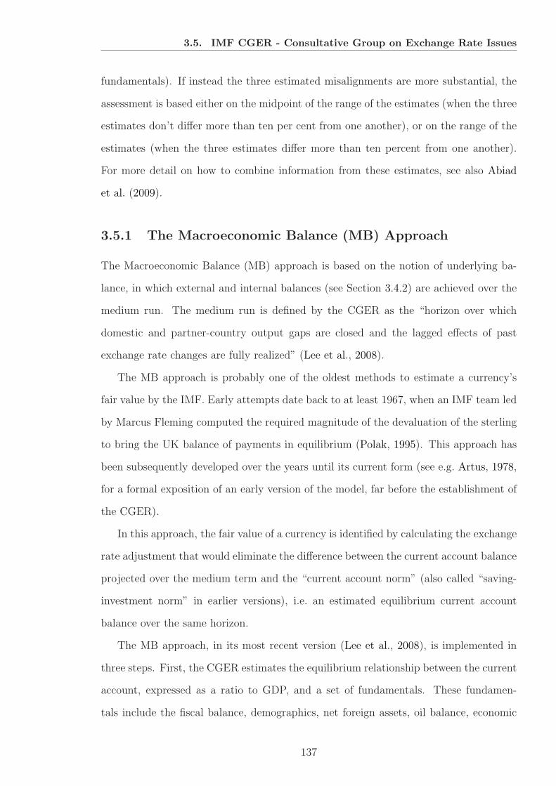
3.5. IMF CGER - Consultative Group on Exchange Rate Issues
fundamentals). If instead the three estimated misalignments are more substantial, the
assessment is based either on the midpoint of the range of the estimates (when the three
estimates don’t differ more than ten per cent from one another), or on the range of the
estimates (when the three estimates differ more than ten percent from one another).
For more detail on how to combine information from these estimates, see also Abiad
et al. (2009).
3.5.1 The Macroeconomic Balance (MB) Approach
The Macroeconomic Balance (MB) approach is based on the notion of underlying ba-
lance, in which external and internal balances (see Section 3.4.2) are achieved over the
medium run. The medium run is defined by the CGER as the “horizon over which
domestic and partner-country output gaps are closed and the lagged effects of past
exchange rate changes are fully realized” (Lee et al., 2008).
The MB approach is probably one of the oldest methods to estimate a currency’s
fair value by the IMF. Early attempts date back to at least 1967, when an IMF team led
by Marcus Fleming computed the required magnitude of the devaluation of the sterling
to bring the UK balance of payments in equilibrium (Polak, 1995). This approach has
been subsequently developed over the years until its current form (see e.g. Artus, 1978,
for a formal exposition of an early version of the model, far before the establishment of
the CGER).
In this approach, the fair value of a currency is identified by calculating the exchange
rate adjustment that would eliminate the difference between the current account balance
projected over the medium term and the “current account norm” (also called “saving-
investment norm” in earlier versions), i.e. an estimated equilibrium current account
balance over the same horizon.
The MB approach, in its most recent version (Lee et al., 2008), is implemented in
three steps. First, the CGER estimates the equilibrium relationship between the current
account, expressed as a ratio to GDP, and a set of fundamentals. These fundamen-
tals include the fiscal balance, demographics, net foreign assets, oil balance, economic
137

3.5. IMF CGER - Consultative Group on Exchange Rate Issues
growth, and dummies for economic crises and financial centers (for extensive studies of
the medium-term determinants of current accounts, see also Debelle and Faruqee, 1996,
and Chinn and Prasad, 2003). The medium-term equilibrium relationship is estimated
via panel data regressions, using four-year averages of the data.
The second step is to compute current account norms by applying the estimated
coefficients of the panel regression to the medium-term values of the regressors. These
medium-term values are mostly taken from the IMF’s World Economic Outlook (WEO)
database, and are generated by IMF’s country experts.
The third step involves computing the real exchange rate adjustment that would
close the gap between the current account norm (estimated in the first two steps) and
the underlying current account (UCUR) balance. In the CGER setting, the IMF WEO
medium-term projection of the level of the current account is taken as the estimate of the
underlying current account balance. This projection assumes that economies operate at
full potential output and the effect of lagged exchange rates has vanished. Projections
for different countries are based on different models, reflecting country-specific views
of IMF experts. Therefore, a drawback of this approach is that it may lack of global
consistency.
An alternative to the WEO projections would be to employ a standard trade model in
order to estimate the UCUR balance, as in previous versions of the MB approach (Isard
and Faruqee, 1998; Isard et al., 2001). Typically, such (multiple-equation) trade model
would specify imports as a function of domestic GDP and past real exchange rates, and
exports as a function of a trade-weighted average of foreign GDP and past real exchange
rates. Underlying exports and imports (and therefore the UCUR as measured as net
underlying exports) would then be calculated by applying the estimated coefficients to
the value of domestic and foreign activity at potential output levels, once the effect of
exchange rates has fully realised (see also Isard, 2007). Even though CGER assessments
rely now only on WEO projections in order to estimate the underlying current account
balance, a similar trade model is still used in order to estimate the trade elasticities
which are needed to calculate the exchange rate adjustment.
138
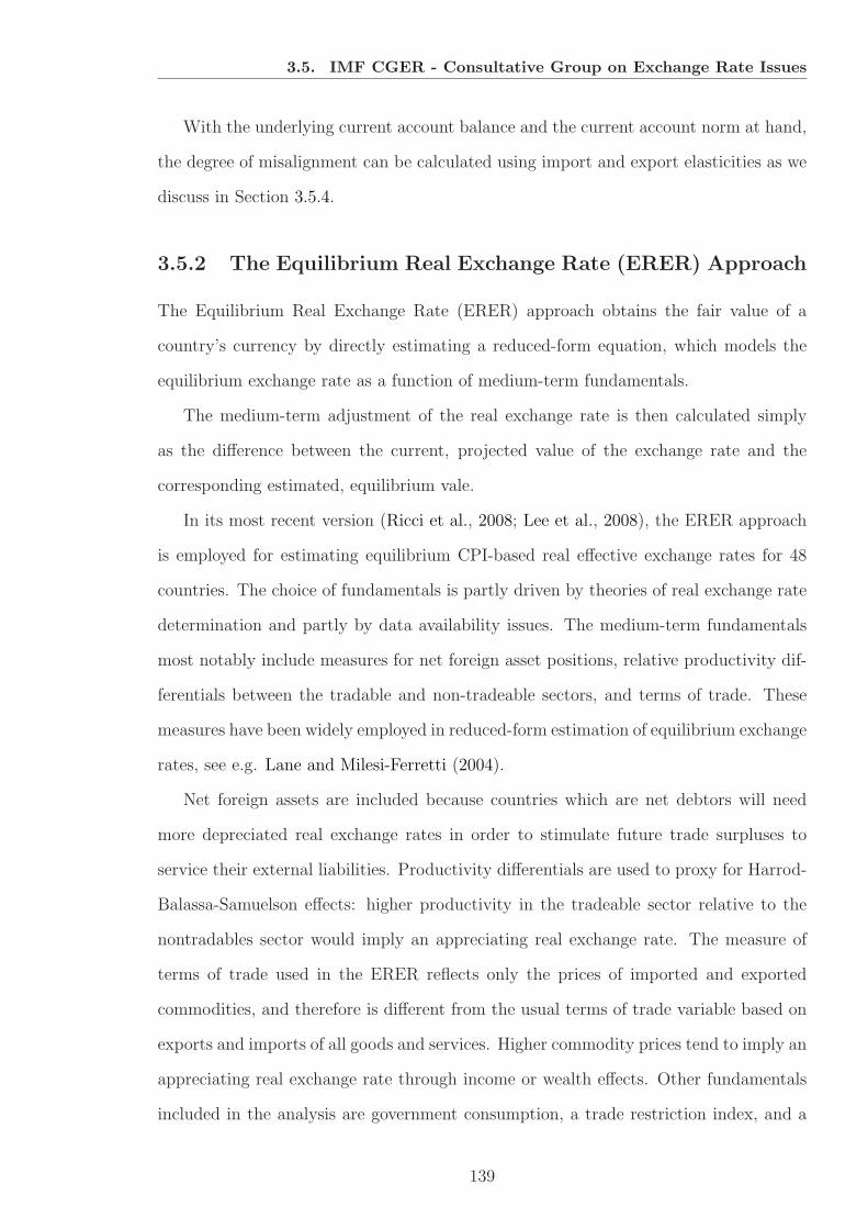
3.5. IMF CGER - Consultative Group on Exchange Rate Issues
With the underlying current account balance and the current account norm at hand,
the degree of misalignment can be calculated using import and export elasticities as we
discuss in Section 3.5.4.
3.5.2 The Equilibrium Real Exchange Rate (ERER) Approach
The Equilibrium Real Exchange Rate (ERER) approach obtains the fair value of a
country’s currency by directly estimating a reduced-form equation, which models the
equilibrium exchange rate as a function of medium-term fundamentals.
The medium-term adjustment of the real exchange rate is then calculated simply
as the difference between the current, projected value of the exchange rate and the
corresponding estimated, equilibrium vale.
In its most recent version (Ricci et al., 2008; Lee et al., 2008), the ERER approach
is employed for estimating equilibrium CPI-based real effective exchange rates for 48
countries. The choice of fundamentals is partly driven by theories of real exchange rate
determination and partly by data availability issues. The medium-term fundamentals
most notably include measures for net foreign asset positions, relative productivity dif-
ferentials between the tradable and non-tradeable sectors, and terms of trade. These
measures have been widely employed in reduced-form estimation of equilibrium exchange
rates, see e.g. Lane and Milesi-Ferretti (2004).
Net foreign assets are included because countries which are net debtors will need
more depreciated real exchange rates in order to stimulate future trade surpluses to
service their external liabilities. Productivity differentials are used to proxy for Harrod-
Balassa-Samuelson effects: higher productivity in the tradeable sector relative to the
nontradables sector would imply an appreciating real exchange rate. The measure of
terms of trade used in the ERER reflects only the prices of imported and exported
commodities, and therefore is different from the usual terms of trade variable based on
exports and imports of all goods and services. Higher commodity prices tend to imply an
appreciating real exchange rate through income or wealth effects. Other fundamentals
included in the analysis are government consumption, a trade restriction index, and a
139
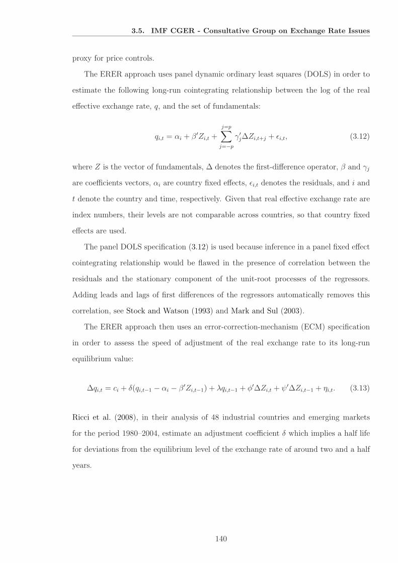
3.5. IMF CGER - Consultative Group on Exchange Rate Issues
proxy for price controls.
The ERER approach uses panel dynamic ordinary least squares (DOLS) in order to
estimate the following long-run cointegrating relationship between the log of the real
effective exchange rate, q, and the set of fundamentals:
qi,t = αi + β′Zi,t +
j=p∑
j=−p
γ′j∆Zi,t+j + ǫi,t, (3.12)
where Z is the vector of fundamentals, ∆ denotes the first-difference operator, β and γj
are coefficients vectors, αi are country fixed effects, ǫi,t denotes the residuals, and i and
t denote the country and time, respectively. Given that real effective exchange rate are
index numbers, their levels are not comparable across countries, so that country fixed
effects are used.
The panel DOLS specification (3.12) is used because inference in a panel fixed effect
cointegrating relationship would be flawed in the presence of correlation between the
residuals and the stationary component of the unit-root processes of the regressors.
Adding leads and lags of first differences of the regressors automatically removes this
correlation, see Stock and Watson (1993) and Mark and Sul (2003).
The ERER approach then uses an error-correction-mechanism (ECM) specification
in order to assess the speed of adjustment of the real exchange rate to its long-run
equilibrium value:
∆qi,t = ci + δ(qi,t−1 − αi − β′Zi,t−1) + λqi,t−1 + φ′∆Zi,t + ψ′∆Zi,t−1 + ηi,t. (3.13)
Ricci et al. (2008), in their analysis of 48 industrial countries and emerging markets
for the period 1980–2004, estimate an adjustment coefficient δ which implies a half life
for deviations from the equilibrium level of the exchange rate of around two and a half
years.
140

3.5. IMF CGER - Consultative Group on Exchange Rate Issues
3.5.3 The External Sustainability (ES) Approach
The CGER External Sustainability (ES) approach calculates the equilibrium real ex-
change rate that would bring the current account or trade balance from its projected
medium-term level to the level that would stabilise the net foreign assets position of
a country. Unlike the MB and ERER approaches, the ES approach requires only few
inputs (such as the prevailing growth and rates of return on external assets and liabi-
lities) to be implemented, without the need of any direct econometric estimations of
equilibrium relations.
The concept of external sustainability is analogous to the one of public debt sustaina-
bility, but with the object of the analysis being the whole economy instead of the public
sector alone. According to the IMF, external sustainability is reached when a country
meets its intertemporal budget constraint (see e.g. IMF, 2002, 2008), which implies that
the net present value (NPV) of future current account or trade surpluses balances must
be equal or greater than the NPV of that country’s external liabilities. This condition
is automatically met when the debt-to-GDP ratio is either stable or declining.
The intertemporal budget constraint is
Bt −Bt−1 = CAt +KGt + Et, (3.14)
where B denotes net foreign assets, CA is the current account, KG is the net capital
gain on the existing holding of foreign assets and liabilities, and E represents capital
account transfers and errors and omissions. Assuming that the latter two factors are
negligible and therefore setting them equal to zero, and denoting ratios to nominal GDP
with lower case letters, we can write Equation (3.14) as
bt − bt−1 = cat −gt + πt(1 + gt)
(1 + gt)(1 + πt)bt−1, (3.15)
where g is the growth rate or real GDP and π is the rate of change of the GDP deflator.
We can express current account cas which stabilises NFA positions to a predetermined
141

3.5. IMF CGER - Consultative Group on Exchange Rate Issues
level bs by setting bt − bt−1 to zero, so that from the previous equation
caS =g + π(1 + g)
(1 + g)(1 + π)bS. (3.16)
Analogously, we can apply the same approach to compute the NFA stabilising trade
balance. Denoting the gross real interest rates as (1 + r) = (i+i)(1+π)
, we can write the
NFA-stabilizing trade balance (inclusive of services and transfers) as
tbS = −r − g
1 + gbS. (3.17)
Therefore, given the assumed values for g, π, and r, the NFA-stabilizing current accounts
and trade balances can be readily computed without the econometric estimation of
any equilibrium relation. Clearly, a drawback of this approach is that the choice of
benchmark level of NFA, bS, will be to some extent arbitrary.
We can compare the NFA-stabilising values of CAS and TBS obtained using equa-
tions (3.16) and (3.17) to their actual values, and apply the same trade elasticities as for
the MB approach in order to calculate the required change in the real effective exchange
rate (see also Section 3.5.4).
Given their simplicity, equations (3.16) and (3.17) have straightforward implications.
For example, the NFA-stabilizing current account is proportional to the GDP growth
rate, so that a faster-growing economy can afford to run larger current account deficits.
Moreover, if the rate of return on external assets and liabilities is greater than the GDP
growth rate, an increase in the former implies, ceteris paribus, a larger trade surplus for
a debtor country whereas a creditor country can afford larger trade deficits (with this
relation being inversed if the rate of return is less than the growth rate).
3.5.4 The Importance of Trade Elasticities
The MB approach and the ES approach really only differ in the way they estimate—or
calculate—the current account target. In a second step, both models use an identical
procedure to calculate the needed exchange rate ajustment for the current account to
142
3.5. IMF CGER - Consultative Group on Exchange Rate Issues
reach this target.
Countries with high ratios of exports and imports to GDP (i.e. countries which are
more open to trade), will require smaller exchange rate adjustments in order to achieve
current accounts consistent with macroeconomic balance. This effect can be seen from
Figure 3.1: an increase in trade openness, other things being equal, will tend to flatten
the UCUR line, resulting in a smaller movement in the real effective exchange rate to
move from the current level REER1 to the equilibrium level REER∗. Aanalytically,
denoting the trade-balance-to-GDP ratio as tb, we have that
tb =PXX
GDP−PMM
GDP, (3.18)
where M and X are import and export volumes, and PM and PX are prices of imports
and exports in local currency.8 The total differential of tb with respect to the real
exchange rate Q is
∂tb
∂Q=∂X
∂Q
PX
GDP+∂PX
∂Q
X
GDP−∂M
∂Q
PM
GDP−∂PM
∂Q
M
GDP. (3.19)
Assuming that exports are priced in local currency (so that ∂PX
∂Q= 0) and that imports
are priced in foreign currency (so that they are unit elastic with respect to Q, ∂PM
∂Q=
−PM
Q), we have that Equation (3.19) can be rewritten as
∂tb
(∂Q)/Q= ηX
PXX
GDP− (ηM − 1)
PMM
GDP, (3.20)
where ηX = ∂X∂Q
QX
is the export elasticity and ηM = ∂M∂Q
QM
is the import elasticity, with
ηX < 0 and ηM > 0. This implies that, for given export and import elasticities, the
impact of a change in the exchange rate will be roughly proportional to trade openness.
This calculation tends to be sensitive with respect to the estimated trade elasticities—
a small error in the estimation of the trade elasticities can potentially lead to calculated
exchange rate adjustment which may differ significantly to the true value, or even have
8In what follows, we assume that the trade balance is the sole source of current account adjustments,consistently with the IMF approach.
143

3.6. Goldman Sachs GSDEER
a counterintuitive sign. This is a particularly important issue, as trade elasticities tend
to be difficult to estimate. For example, Cheung et al. (2010) report a wide range of
estimated exports and imports elasticities for China, based both on previous studies
and their own calculations.
Furthermore, the empirical evidence regarding the Marshall-Lerner condition is mixed.
Several studies find supporting evidence for selected countries over longer horizons, but
considerable doubts remain in particular with regard to shorter term dynamics (see e.g.
Rose, 1991; Hsing, 2010).
Table 3.1 illustrates the point and presents, for given trade elasticities, the percentage
change in the real effective exchange rate which is required to bring China’s underlying
current account in line with the current account target. The required change is computed
using formula (3.20). We use the current account projections for 2016 from the IMF
WEO of April 2011 as an estimate of the underlying current account balance. We
estimate the 2010 China’s exports/GDP and imports/GDP ratios as 29.8 and 25.9
percent, respectively. Data for these ratios are from China’s national statistics and the
IMF. For illustrative purposes, we do not estimate here the current account target (as
opposed to the CGER approach) but assume two different levels. Panel A shows the
results assuming a current account target of zero percent, whereas Panel B shows the
results assuming a current account target of three percent. The table clearly shows that
MB calculations are extremely sensitive with respect to the estimated trade elasticities,
in particular when they approach the region where the Marshall-Lerner condition is
no longer satisfied. In this simple example, the required exchange rate adjustments
can differ for figures as high as 2300 percent for only a 0.1 change in the estimated
elasticities.
3.6 Goldman Sachs GSDEER
Similar to the work of the IMF on exchange rates, Goldman Sachs has been using
a family of fair value models, which have followed different concepts and which have
changed over time. In this section, we first describe the models and then discuss in
144

3.6. Goldman Sachs GSDEER
more detail the specific adjustments applied to the latest generation of the GSDEER
model.
3.6.1 The Evolution of the GSDEER Model
The first version of GSDEER was introduced in the mid 1990s (Goldman Sachs, 1996)
and was a simple adjusted-PPP model allowing for Harrod-Balassa-Samuelson effects.
The coefficient on productivity was assumed to be unity. The model was not estimated
but in fact calculated by applying inflation and productivity differentials to an initial
reference period, at which the bilateral exchange rates were assumed to be in equili-
brium. The latter was determined by judgment with strong focus on the size of current
account imbalances. Calculated misalignment values where available for the currencies
of advanced economies.
At the same time, Goldman Sachs developed a second fair value model for Emerging
Market currencies,9 which was essentially a BEER model with a relatively large number
of model inputs reflecting external sustainability—a choice driven by the fact that EM
currency crises were frequent at the time. Specifically, the following variables were used:
terms of trade, the degree of openness to foreign trade, the share of long-term capital
inflows as a percentage of GDP, the amount and composition of government spending
and the level of international interest rates (Goldman Sachs, 1996).
These two models were merged into a unified BEER-style approach estimated with
panel DOLS cointegration techniques with country fixed effects (O’Neill et al., 2005).
More specifically, the real bilateral exchange rate was estimated as a function of terms
of trade differentials, productivity differentials and the relative net foreign asset position
between two countries. The real exchange rate was calculated using CPI indices. The
coefficient estimates were highly significant except for the net foreign asset position.
Given that the model is estimated in a panel for approximately 30 currencies, the
choice of variables is partly driven by the availability of data. To allow out-of-sample
9This model was called the Goldman Sachs Dynamic Equilibrium Emerging Markets Exchange Rate(GSDEEMER) model.
145

3.6. Goldman Sachs GSDEER
projections of fair value estimates, Goldman uses its in-house forecasts for the input
variables.
This generation of GSDEER model has been re-estimated about every two years
with some modifications at each iteration. Recently the net foreign asset variable has
been dropped as its significance dropped further and given that the signs flipped and be-
came counterintuitive, indicating that rising external liabilities were associated with an
appreciating fair value (Fuentes and Meechan, 2007). The authors faced the challenges
linked to external balance variables discussed in Section 3.3.3 and decided to drop the
variable altogether. As a result, the GSDEER fair value estimates now do not depend
on variables of external imbalances.
3.6.2 Level Adjustments Based on the Penn effect
Another major issue relates to what we discussed in Section 3.3.2: short samples for
some countries or a history of managed exchange rates for others may severely bias
the estimation of the intercept of reduced form fair value models. In turn, errors in the
estimation of the intercept will translate in a biased estimate of the fair value level of the
exchange rate. In the latest version of the GSDEER model, Goldman’s economists (see
Stolper et al., 2009) argue that most of the data problems leading to a biased estimate of
the intercept will also lead to the violation of the assumption of cointegration between
the exchange rates and the fundamentals. They test this assumption by testing the
stationarity of the cross-sectional residuals. Their results show that the hypothesis of a
unit root in the residuals is particular unlikely to get rejected for:
• currencies with a history of managed exchange rates, typically in developing Asia;
• currencies which have been subject to periods of hyperinflation and the related
data quality issues, typically in Latin America;
• currencies with short samples, in particular in Central and Eastern Europe.
For those cases in which the unit-root hypothesis cannot be rejected, Stolper et al.
(2009) adjust the country fixed effects of the GSDEER model by estimating a cross-
146

3.6. Goldman Sachs GSDEER
sectional model based on the Penn effect, as the one described in Section 3.4.1. Figure
3.4 shows time series of nominal GSDEER fair values (against the US dollar) for the
euro, the British pound, the Japanese yen, and the Chinese renminbi. Of these four fair
values, only the renminbi has been subject to a level correction based on the Penn effect
correction.
3.6.3 Penn effects and the Size of Agricultural Sector
When estimating the Penn effect, Stolper et al. (2009) make the explicit choice to
adjust the income-per-capita variable for non-agricultural sectors of the economy. This
adjustment is worth a more detailed explanation.
As discussed in Section 3.4.1, the Penn effect is based on productivity differentials
between the non-tradable and the tradable sectors. Assuming that productivity in the
non-tradable sector is comparable across countries, the deviations from PPP can be
shown to be a function of cross country differential in tradable sector productivity.
In typical empirical estimates of the Penn effect, it is assumed that GDP-per-capita
differentials are proportional to tradable sector productivity differentials. However, this
makes the implicit assumption that the tradable sector is of comparable size across
countries—an assumption that is frequently violated, in particular in countries with
large agricultural sectors.
To illustrate the importance of this adjustment in the GSDEER, we estimate the
Penn effect as in Equation (3.5), but calculating GDP-per-capita variable in three dif-
ferent ways: (i) unadjusted, (ii) adjusted for output and employment in primary and
secondary sector, i.e. excluding agriculture, and (iii) adjusted for the industrial sector
alone. To make the adjustment, we use World Bank data on the employment and output
shares of the individual sectors.
The three estimates are quite comparable in fit (see Table 3.2), but when calculating
fitted values for the currencies of countries with large agricultural sectors, substantial
differences arise. Figure 3.5 illustrates this point for the case of the Chinese renminbi,
and shows differences in estimated misalignments varying by up to nine percentage
147

3.7. Conclusion
points. The estimated undervaluation for the renminbi reached 15 percent in 2003
when using the adjusted measure of GDP-per-capita for the industrial sector. When
we consider instead the unadjusted measure, the estimates show at most six percent
undervaluation during the same period.
3.7 Conclusion
A primitive notion of currency misalignment linked to the precious metal content of
coins has probably been around since the antiquity. The notion that prices of tradable
goods are unlikely to diverge substantially across countries can be traced back several
centuries and remains a key building block of modern adjusted-PPP or BEER models.
Similarly, the link between currency valuation and external imbalances—in particular
the impact on foreign exchange reserves—has been observed in Roman times and remains
an important building block of the many variants of modern underlying balance models.
In this chapter we review the most important families of fair value models currently
in use. Most of these models have been developed over the last 20 years. Moreover,
we introduce the concept of Indirect Fair Value (IFV), a notion of fair value frequently
used by financial market participants for short-term investment decisions, but to our
knowledge not previously formalised in the academic literature.
Currency fair value modelling has always been a field of interest for policymakers
and investors and fair value estimates are frequently an input for important political
or financial decisions. As a result, it is important to highlight the implicit or explicit
modelling and implementation choices. Given important trade-offs when choosing a
fair value model, many practitioners now combine several models and approaches to
correct or compensate for individual weaknesses. Both our case studies, the IMF GER
framework and the Goldman Sachs GSDEER models, follow that path.
In the context of these case studies, we illustrate empirically how some of the model-
ling choices affect fair value estimates. Specifically, we show the sensitivity of underlying
balance models to import and export elasticities. Moreover, we estimate three variants
of a Penn-Effect model and show the sensitivity to implicit assumptions about the re-
148

3.7. Conclusion
lative size of the non-tradable sector in the economy.
149

3. Tables
Table 3.1. Real Effective Exchange Rate Adjustment for China, Sensitivity Ana-lysis
The table presents, for given trade elasticities, the percentage change in the real effectiveexchange rate which is required to bring China’s underlying current account in line with thecurrent account target. The required change is computed using Equation (3.20) in the maintext. We use the current account projections for 2016 from the IMF WEO of April 2011as an estimate of the underlying current account balance. We estimate the 2010 China’sexports/GDP and imports/GDP ratios as 29.8 and 25.9 percent, respectively. Data for theseratios are from China’s national statistics and the IMF. Panel A shows the results assuming acurrent account target of zero percent, whereas Panel B shows the results assuming a currentaccount target of 3 percent.
Panel A: 0% Current Account Target
Export Elasticities
-0.1 -0.2 -0.3 -0.4 -0.5 -0.6 -0.7 -0.8 -0.9 -1.0
Import
Elasticities
0.1 -38.4 -45.0 -54.3 -68.5 -92.7 -143.6 -318.4 1471.7 222.2 120.2
0.2 -44.0 -52.8 -66.2 -88.6 -134.0 -274.6 5571.4 250.0 127.9 85.9
0.3 -51.5 -64.1 -84.9 -125.6 -241.5 -3120.0 285.7 136.6 89.8 66.8
0.4 -62.1 -81.4 -118.2 -215.5 -1218.8 333.3 146.6 94.0 69.1 54.7
0.5 -78.2 -111.6 -194.5 -757.3 400.0 158.2 98.6 71.6 56.2 46.3
0.6 -105.7 -177.3 -549.3 500.0 171.8 103.7 74.3 57.9 47.4 40.1
0.7 -162.8 -430.9 666.7 188.0 109.4 77.2 59.6 48.5 40.9 35.4
0.8 -354.5 1000.0 207.4 115.7 80.2 61.4 49.7 41.8 36.0 31.7
0.9 2000.0 231.5 122.8 83.6 63.4 51.0 42.7 36.7 32.2 28.7
1.0 261.7 130.9 87.2 65.4 52.3 43.6 37.4 32.7 29.1 26.2
Panel B: 3% Current Account Target
Export Elasticities
-0.1 -0.2 -0.3 -0.4 -0.5 -0.6 -0.7 -0.8 -0.9 -1.0
Import
Elasticities
0.1 -23.6 -27.7 -33.4 -42.1 -57.1 -88.4 -195.9 905.7 136.8 74.0
0.2 -27.1 -32.5 -40.7 -54.5 -82.5 -169.0 3428.6 153.8 78.7 52.9
0.3 -31.7 -39.4 -52.2 -77.3 -148.6 -1920.0 175.8 84.1 55.2 41.1
0.4 -38.2 -50.1 -72.7 -132.6 -750.0 205.1 90.2 57.8 42.6 33.7
0.5 -48.1 -68.7 -119.7 -466.0 246.2 97.4 60.7 44.1 34.6 28.5
0.6 -65.0 -109.1 -338.0 307.7 105.7 63.8 45.7 35.6 29.2 24.7
0.7 -100.2 -265.2 410.3 115.7 67.3 47.5 36.7 29.9 25.2 21.8
0.8 -218.2 615.4 127.7 71.2 49.4 37.8 30.6 25.7 22.2 19.5
0.9 1230.8 142.4 75.6 51.4 39.0 31.4 26.3 22.6 19.8 17.6
1.0 161.1 80.5 53.7 40.3 32.2 26.8 23.0 20.1 17.9 16.1
150

3. Tables
Table 3.2. Penn effect adjustment in GSDEER, different sectors
The table presents the regression results for the Penn effect adjustment in the GSDEER forthe Chinese renminbi against the US dollar.
All sectors Industry Industry plus Services
Coefficient 0.343 0.428 0.421t-statistic 25.745 24.637 27.135R2 0.478 0.455 0.504
151

3. Figures
Current
Account
Real Effective
Exchange Rate
Underlying
Current Account
Balance
Current Account
Norm
0
REER1
REER*
UCUR1
SurplusDeficit
Figure 3.1. Underlying Balance Approach
The figure illustrates the Underlying Balance approach described in the main text.
152

3. Figures
2004 2005 2006 2007−0.6
−0.5
−0.4
−0.3
−0.2
−0.1
0
0.1
0.2
0.3
0.4
Year
Ris
k R
ever
sals
Figure 3.2. USD/CAD 3-month 25-Delta Risk reversals
Notes: The figure shows risk reversals for 3-month 25-Delta out-of-the-money options for theCanadian dollar against the US dollar.
153

3. Figures
2004 2005 2006 20071
1.05
1.1
1.15
1.2
1.25
1.3
1.35
1.4
Year
US
D/C
AD
Exc
hang
e R
ate
FittedRealisedFair Value
Figure 3.3. Indirect Fair Value for USD/CAD
The figure illustrates the Indirect Fair Value (IFV) for the daily nominal spot exchange rateof the Canadian dollar against the US dollar. The time span is between January 2004 andJanuary 2007. The black line displays the actual observed value of the exchange rate. Thelight grey line displays the fitted value of a regression of the spot exchange rate on: thedifference between US and Canadian 2-year swap rates; linear, quadratic, and cubic timetrends; and 3-month 25-Delta risk reversals. Finally, the dark grey line displays the IFV of theCanadian dollar, using the sample mean of the risk reversals as a proxy for neutral speculativepositioning.
154

3. Figures
1985 1990 1995 2000 2005 20100.4
0.6
0.8
1
1.2
1.4
1.6
1.8
Year
US
D/E
UR
ObservedGSDEER
USD/EUR
1975 1980 1985 1990 1995 2000 2005 20101
1.5
2
2.5
Year
US
D/G
BP
ObservedGSDEER
USD/GBP
1975 1980 1985 1990 1995 2000 2005 201050
100
150
200
250
300
350
Year
JPY
/US
D
ObservedGSDEER
JPY/USD
1990 1995 2000 2005 20104
4.5
5
5.5
6
6.5
7
7.5
8
8.5
9
Year
CN
Y/U
SD
ObservedGSDEER
CNY/USD
Figure 3.4. GSDEER Fair Values
The figure shows the observed nominal exchange rates and the GSDEER fair value estimatesfor a number of currencies.
155

3. Figures
1990 1992 1994 1996 1998 2000 2002 2004 2006 2008 2010−0.2
−0.1
0
0.1
0.2
0.3
0.4
0.5
Year
Mis
alig
nmen
t
All SectorsIndustry onlyIndustry and Services
Figure 3.5. USD/CNY Misalignments for Different Penn Effect Specifications
The figure illustrates the misalignment of the Chinese renminbi against the US dollar fordifferent Penn effect specifications as described in the main text. The solid line displays themisalignment considering all sectors; the dashed line exhibits the misalignment consideringonly the industrial sector; finally, the dash-dot line shows the misalignment considering theindustrial and services sectors together.
156

Chapter 4
Concluding Remarks
The carry trade is a currency investment strategy designed to exploit deviations from
uncovered interest parity. Its profitability is based on the empirical observation that
the interest rate differential across countries is not, on average, offset by a depreciation
of the investment currency. Hence, investing in high-interest currencies by borrowing
from low-interest currencies tends to deliver large positive excess returns.
The first chapter of this thesis fills a gap in the literature by demonstrating empi-
rically the existence of an intertemporal risk-return tradeoff between the return to the
carry trade and risk in a predictive setting. We measure FX risk by the variance of the
returns to the FX market portfolio. We then take a step further by decomposing the
market variance into the cross-sectional average variance and the cross-sectional ave-
rage correlation of exchange rate returns. Our empirical analysis is based on predictive
quantile regressions, which provide a natural way of assessing the effect of higher risk
on different quantiles of the return distribution.
Our main finding is that average variance has a significant negative effect on the
left tail of the distribution of future carry trade returns, whereas average correlation
has a significant negative effect on the right tail. We take advantage of this finding by
forming a new version of the carry trade that conditions on average variance and average
correlation, and show that this strategy performs considerably better than the standard
carry trade. These results imply that to some extent exchange rates are predictable,
especially when it matters most: when the carry trade produces large gains or large
157

Concluding Remarks
losses. In other words, if the carry trade is about “going up the stairs and down the
elevator,” then average variance and average correlation can tell us something valuable
about when the elevator is likely to go up or down. In the end, by focusing on the tails
of the return distribution of carry trades, we uncover a negative risk-return tradeoff in
foreign exchange.
In the second chapter, I analyse the reaction of exchange rates to interest rate diffe-
rentials shocks. Previous literature has shown that exchange rates tend to react sluggi-
shly to shocks, so that a an unexpectedly higher foreign interest rate generates a slow
and persistent appreciation of the foreign currency for several quarters. This finding
implies a violation of a conditional version of UIP and long-run PPP: excess return on
foreign exchange should react instantaneously to an unexpected interest rate shock and
jump to the level implied by the present value of changes in expectations of future real
interest rate differentials.
I argue that previous empirical findings, by mostly ignoring the role of nonlinearities
and the evolution of exchange rates dynamics over time, may have represented only an
average of the past, and not reflected the current state of the economy. Therefore, pre-
vious results may be biased and may not provide useful insights for a currency investor
betting on violations of UIP in a given point in time.
In order to re-examine the evidence of conditional violations of UIP, I employ a Baye-
sian time-varying-parameter VAR which allows for time-variation both in the transmis-
sion mechanism of the shocks and the volatility of the shocks themselves. This frame-
work allows me to estimate the time-varying responses of the excess retuns on foreign
exchange and to compare them to those implied by UIP and long-run PPP, at the same
time explicitly taking into account parameter uncertainty.
I find that the transmission of the interest rate differential shocks has changed over
time. However, even if to a varying degree over the years, some of the puzzling results
previously documented with linear models remain. I show that currency excess returns
tend to initially underreact to interest rate differential shocks for the whole sample
considered, undershooting the level implied by fundamentals. At longer horizons, the
158

Concluding Remarks
previously documented evidence of overshooting tends to disappear in recent years in
the case of the euro, the British pound and the Canadian dollar. Instead, overreaction
at long horizons is a persistent feature of the excess returns on the Japanese yen and
the Swiss franc throughout the whole sample.
These results suggest that previously documented conditional violations of UIP may
have secularly declined over time, at least for euro, the British pound and the Canadian
dollar. However, the results for the Japanese yen and the Swiss franc—two currencies
which have been traditionally used for funding carry trade positions—may hint that
speculation in the foreign exchange market may constitute a destabilizing force, driving
exchange rates away from fundamentals.
In the third chapter we review the most important families of fair value models
currently in use. Most of these models have been developed over the last 20 years.
Moreover, we introduce the concept of Indirect Fair Value (IFV), a notion of fair value
frequently used by financial market participants for short-term investment decisions,
but to our knowledge not previously formalised in the academic literature.
Currency fair value modelling has always been a field of interest for policymakers
and investors and fair value estimates are frequently an input for important political
or financial decisions. As a result, it is important to highlight the implicit or explicit
modelling and implementation choices. Given important tradeoffs when choosing a
fair value model, many practitioners now combine several models and approaches to
correct or compensate for individual weaknesses. Both our case studies, the IMF GER
framework and the Goldman Sachs GSDEER models, follow that path.
In the context of these case studies, we illustrate empirically how some of the model-
ling choices affect fair value estimates. Specifically, we show the sensitivity of underlying
balance models to import and export elasticities. Moreover, we estimate three variants
of a Penn-Effect model and show the sensitivity to implicit assumptions about the re-
lative size of the non-tradable sector in the economy.
159

Bibliography
Abiad, A., Kannan, P., Lee, J., 2009. Evaluating historical CGER assessments: How
well have they predicted subsequent exchange rate movements?, IMF Working Paper.
Abreu, D., Brunnermeier, M. K., 2003. Bubbles and crashes. Econometrica 71, 173–204.
Akram, Q. F., Rime, D., Sarno, L., 2008. Arbitrage in the foreign exchange market:
Turning on the microscope. Journal of International Economics 76, 237–253.
Alberola, E., Cervero, S. G., Lopez, H., Ubide, A., 1999. Global equilibrium exchange
rates: euro, dollar, “ins,” “outs”, and other major currencies in a panel cointegration
framework, IMF Working Paper.
Ang, A., Hodrick, R. J., Xing, Y., Zhang, X., 2006. The cross-section of volatility and
expected returns. Journal of Finance 61, 259–299.
Ang, A., Hodrick, R. J., Xing, Y., Zhang, X., 2009. High idiosyncratic volatility and
low returns: International and further U.S. evidence. Journal of Financial Economics
91, 1–23.
Artus, J. R., 1978. Methods of assessing the long-run equilibrium value of an exchange
rate. Journal of International Economics 8, 277 – 299.
Bacchetta, P., van Wincoop, E., 2004. A scapegoat model of exchange-rate fluctuations.
American Economic Review Papers and Proceedings 94, 114–118.
Bacchetta, P., van Wincoop, E., 2010. On the unstable relationship between exchange
rates and macroeconomic fundamentals, Working Paper.
160

Bibliography
Balassa, B., 1964. The purchasing-power parity doctrine: A reappraisal. Journal of
Political Economy 72, pp. 584–596.
Bali, T. G., 2008. The intertemporal relation between expected returns and risk. Journal
of Financial Economics 87, 101–131.
Bali, T. G., Cakici, N., Yan, X., Zhang, Z., 2005. Does idiosyncratic risk really matter?
Journal of Finance 60, 905–929.
Bali, T. G., Yilmaz, K., 2011. The intertemporal relation between expected return
and risk on currency. In: Lee, C.-F. (Ed.), Handbook of Financial Econometrics
(forthcoming). Springer, New York.
Bandi, F., Perron, B., 2008. Long-run risk-return trade-offs. Journal of Econometrics
143, 349–374.
Bayoumi, T., Clark, P., Symansky, S., Taylor, M., 1994. The robustness of equilibrium
exchange rate calculations to alternative assumptions and methodologies, IMF Wor-
king Paper.
Bekaert, G., 1995. The time variation of expected returns and volatility in foreign ex-
change markets. Journal of Business and Economic Statistics 13, 397–408.
Benati, L., 2008. The “Great Moderation” in the United Kingdom. Journal of Money,
Credit and Banking 40, 121–147.
Bilson, J., 1981. The speculative efficiency hypothesis. Journal of Business 54, 433–451.
Bowley, A., 1920. Elements of Statistics. Scribner’s, New York.
Brunnermeier, M., Nagel, S., Pedersen, L. H., 2009. Carry trades and currency crashes.
NBER Macroeconomics Annual 23, 313–347.
Burnside, C., 2010. Carry trades and risk. In: James, J., Sarno, L., Marsh, I. W. (Eds.),
Handbook of Exchange Rates (forthcoming). Wiley.
161

Bibliography
Burnside, C., Eichenbaum, M., Kleshchelski, I., Rebelo, S., 2011. Do peso problems
explain the returns to the carry trade? Review of Financial Studies 24, 853–891.
Burnside, C., Eichenbaum, M., Rebelo, S., 2008. Carry trade: The gains of diversifica-
tion. Journal of the European Economic Association 6, 581–588.
Campa, J. M., Chang, P. K., Reider, R. L., 1998. Implied exchange rate distributions:
Evidence from OTC option markets. Journal of International Money and Finance 17,
117–160.
Campbell, J. Y., 1991. A variance decomposition for stock returns. The Economic Jour-
nal 101, 157–179.
Carter, C. K., Kohn, R., 1994. On Gibbs sampling for state space models. Biometrika
81, 541–553.
Cassel, G., 1918. Abnormal deviations in international exchanges. The Economic Journal
28, 413–415.
Cenesizoglu, T., Timmermann, A., 2010. Do return prediction models add economic
value?, Working Paper, HEC Montreal.
Chan, K., Karolyi, G., Stulz, R., 1992. Global financial markets and the risk premium
on U.S. equity. Journal of Financial Economics 32, 137–167.
Chen, Z., Petkova, R., 2010. Does idiosyncratic volatility proxy for risk exposure?,
Working Paper, Texas A&M University.
Cheung, Y.-W., Chinn, M. D., Fujii, E., 2007. The overvaluation of renminbi underva-
luation. Journal of International Money and Finance 26, 762–785.
Cheung, Y.-W., Chinn, M. D., Fujii, E., 2009. Pitfalls in measuring exchange rate
misalignment: The yuan and other currencies. Open economies review 20, 183–206.
Cheung, Y.-W., Chinn, M. D., Fujii, E., 2010. China’s current account and exchange
rate. In: Feenstra, R. C., Wei, S.-J. (Eds.), China’s Growing Role in World Trade.
University of Chicago Press, pp. 231–271.
162

Bibliography
Chinn, M. D., 2006. A primer on real effective exchange rates: Determinants, overvalua-
tion, trade flows and competitive devaluation. Open economies review 17, 115–143.
Chinn, M. D., 2011. Macro approaches to foreign exchange determination. In: James, J.,
Sarno, L., Marsh, I. W. (Eds.), Handbook of Exchange Rates (forthcoming). Wiley.
Chinn, M. D., Prasad, E. S., 2003. Medium-term determinants of current accounts in
industrial and developing countries: an empirical exploration. Journal of International
Economics 59, 47–76.
Christiansen, C., 2011. Intertemporal risk-return trade-off in foreign exchange. Journal
of International Financial Markets, Institutions and Money (forthcoming).
Christiansen, C., Ranaldo, A., Soderlind, P., 2011. The time-varying systematic risk of
carry trade strategies. Journal of Financial and Quantitative Analysis (forthcoming).
Clark, P. B., MacDonald, R., 1998. Exchange rates and economic fundamentals: a
methodological comparison of BEERs and FEERs, IMF Working Paper.
Clark, P. B., MacDonald, R., 2004. Filtering the BEER: A permanent and transitory
decomposition. Global Finance Journal 15, 29–56.
Cline, W. R., 2008. Estimating consistent fundamental equilibrium exchange rates, Pe-
terson Institute for International Economics Workin Paper.
Cline, W. R., Williamson, J., 2008. New estimates of fundamental equilibrium exchange
rates, Peterson Institute for International Economics Policy Brief.
Cline, W. R., Williamson, J., 2011. Estimates of fundamental equilibrium exchange
rates, Peterson Institute for International Economics Policy Brief.
Cogley, T., Sargent, T. J., 2001. Evolving post-World War II inflation dynamics. NBER
Macroeconomic Annual 16, 331–373.
Cogley, T., Sargent, T. J., 2005. Drifts and volatilities: monetary policies and outcomes
in the post WWII US. Review of Economic Dynamics 8, 262–362.
163

Bibliography
Cumby, R. E., Huizinga, J., 1990. The predictability of real exchange rate changes in
the short run and the long run, NBER Working Paper No. 3468.
De Broeck, M., Sløk, T., 2006. Interpreting real exchange rate movements in transition
countries. Journal of International Economics 68, 368–383.
Debelle, G., Faruqee, H., 1996. What determines the current account? A cross-sectional
and panel approach, IMF Working Paper.
Della Corte, P., Sarno, L., Tsiakas, I., 2009. An economic evaluation of empirical ex-
change rate models. The Review of Financial Studies 22, 3491–3530.
Deutsche Bank, 2007. Deutsche Bank guide to currency indices.
Dickey, D. A., Fuller, W. A., 1979. Distribution of the estimators for autoregressive time
series with a unit root. Journal of the American Statistical Association 74, 427–431.
Diebold, F. X., Nerlove, M., 1989. The dynamics of exchange rate volatility: A multi-
variate latent factor ARCH model. Journal of Applied Econometrics 4, 1–21.
Dornbusch, R., 1976. Expectations and exchange rate dynamics. The Journal of Political
Economy 84, 1161–1176.
Dornbusch, R., Goldfajn, I., Valdes, R. O., 1995. Currency crises and collapses. Broo-
kings Papers on Economic Activity 26, 219–294.
Driver, R. L., Westaway, P. F., 2004. Concepts of equilibrium exchange rates, Bank of
England Working Paper no. 248.
Du, Q., Wei, S.-J., 2011. Sex ratios and exchange rates, NBER Working Paper No.
16788.
Dumas, B., 1992. Dynamic equilibrium and the real exchange rate in a spatially sepa-
rated world. The Review of Financial Studies 5, 153–180.
Dunis, C., Lequeux, P., 2001. The information content of risk reversals. Derivatives Use,
Trading & Regulation 2, 98–117.
164
Bibliography
Eichenbaum, M., Evans, C. L., 1995. Some empirical evidence on the effects of shocks
to monetary policy on exchange rates. The Quarterly Journal of Economics 110, 975–
1009.
Elliott, G., Muller, U. K., 2006. Efficient tests for general persistent time variation in
regression coefficients. Review of Economic Studies 73, 907–940.
Engel, C., 1996. The forward discount anomaly and the risk premium: A survey of
recent evidence. Journal of Empirical Finance 3, 123–192.
Engel, C., 2010. The real exchange rate, real interest rates, and the risk premium,
Working Paper.
Engel, C., 2011. Currency misalignments and optimal monetary policy: a reexamination.
American Economic Review (forthcoming).
Engel, C., West, K. D., 2005. Exchange rates and fundamentals. Journal of Political
Economy 113, 485–517.
Engel, C., West, K. D., 2010. Global interest rates, currency returns, and the real value
of the dollar. American Economic Review: Papers & Proceedings 100, 562–567.
Engle, R. F., Granger, C. W. J., 1987. Co-integration and error correction: representa-
tion, estimation and testing. Econometrica 55, 251–276.
Fama, E. F., 1984. Forward and spot exchange rates. Journal of Monetary Economics
14, 319–338.
Fama, E. F., French, K. R., 1993. Common risk factors in the returns on stocks and
bonds. Journal of Financial Economics 33, 3–56.
Farhi, E., Fraiberger, S., Gabaix, X., Ranciere, R., Verdelhan, A., 2009. Crash risk in
currency markets, Working Paper, Harvard University.
Faruqee, H., 1998. Methodology for calculating equilibrium exchange rates and question
of global consistency. In: Isard, P., Faruqee, H. (Eds.), Exchange Rate Assessment:
165

Bibliography
Extensions of the Macroeconomic Balance Approach. IMF Occasional Papers. Inter-
national Monetary Fund, Washington.
Faust, J., Rogers, J. H., 2003. Monetary policy’s role in exchange rate behavior. Journal
of Monetary Economics 50, 1403–1424.
Fitzenberger, B., 1997. The moving block bootstrap and robust inference for linear least
squares and quantile regressions. Journal of Econometrics 82, 235–287.
Fleming, J. M., 1962. Domestic financial policies under fixed and floating exchange
rates”. International Monetary Fund Staff Papers 9, 369–379.
Frankel, J., 2006. On the yuan: The choice between adjustment under a fixed exchange
rate and adjustment under a flexible rate. CESifo Economic Studies 52, 246–275.
Frankel, J. A., Rose, A. K., 1995. Empirical research on nominal exchange rates. In:
Grossman, G. M., Rogoff, K. (Eds.), Handbook of International Economics. Vol. 3.
Elsevier, Ch. 33, pp. 1689–1729.
French, K. R., Schewert, W., Satmbaugh, R. F., 1987. Expected stock returns and
volatility. Journal of Financial Economics 19, 3–29.
Frenkel, J. A., 1981. The collapse of purchasing power parities during the 1970’s. Euro-
pean Economic Review 16, 145–165.
Froot, K. A., Ramadorai, T., 2005. Currency returns, intrinsic value, and institutional-
investor flows. The Journal of Finance 60, 1535–1566.
Fuentes, M., Meechan, M., 2007. The evolving GSDEER currency model. Global view-
point, Goldman Sachs.
Funabashi, Y., 1988. Managing the Dollar: from the Plaza to the Louvre. Institute for
International Economics, Washington.
Egert, B., Halpern, L., MacDonald, R., 2006. Equilibrium exchange rates in transition
economies: Taking stock of the issues. Journal of Economic Surveys 20, 257–324.
166
Bibliography
Ghysels, E., Santa-Clara, P., Valkanov, R., 2005. There is a risk-return trade-off after
all. Journal of Financial Economics 76, 509–548.
Giorgianni, L., 1997. Foreign exchange risk premium: Does fiscal policy matter? Evi-
dence from Italian data, IMF Working Paper .
Glosten, L. R., Jagannathan, R., Runkle, D. E., 1993. On the relationship between the
expected value and the volatility of the nominal excess return on stocks. Journal of
Finance 48, 1779–1801.
Goldberg, L. S., Kolstad, C. D., 1995. Foreign direct investment, exchange rate varia-
bility and demand uncertainty. International Economic Review 36, 855–873.
Goldman Sachs, 1996. The foreign exchange market 1996.
Goldman Sachs, 2009. FX slices become new tradable FX currents, Global Viewpoint
09/12.
Gonzalo, J., Granger, C. W. J., 1995. Estimation of common long-memory components
in cointegrated systems. Journal of Business and Economic Statistics 13, 27–35.
Gourinchas, P.-O., Obstfeld, M., 2011. Stories of the twentieth century for the twenty-
first. American Economic Journal: Macroeconomics (forthcoming).
Goyal, A., Santa-Clara, P., 2003. Idiosyncratic risk matters! Journal of Finance 63,
975–1007.
Goyal, A., Saretto, A., 2009. Cross-section of option returns and volatility. Journal of
Financial Economics 94, 310–326.
Gupta, P., Mishra, D., Sahay, R., 2007. Behavior of output during currency crises.
Journal of International Economics 72, 428–450.
Hamilton, J. D., 1994. Time Series Analysis. Princeton University Press.
Harrod, R., 1933. International Economics. James Nisbet.
167
Bibliography
Hsing, Y., 2010. Test of the Marshall-Lerner condition for eight selected Asian countries
and policy implications. Global Economic Review 38, 205–214.
Huizinga, J., 1987. An empirical investigation of the long run behaviour of real exchange
rates. Carnegie-Rochester Conference Series on Public Policy 27, 149–214.
IEO, 2007. The equilibrium exchange rate: alternative concepts and their applications
in IMF surveillance. IMF exchange rate policy advice evaluation report, Independent
Evaluation Office of the International Monetary Fund.
IMF, 2002. Assessing sustainability. Tech. rep., Policy Development and Review De-
partment, International Monetary Fund.
IMF, 2007. Bilateral surveillance over members’ policies, International Monetary Fund
Executive Board Decision.
IMF, 2008. Staff guidance note on debt sustainability analysis for market access coun-
tries. Tech. rep., Policy Development and Review Department, International Mone-
tary Fund.
IMF, 2011. World Economic Outlook. April.
Isard, P., 2007. Equilibrium exchange rates: Assessment methodologies, IMF Working
Paper.
Isard, P., Faruqee, H., 1998. Exchange rate assessment: Extension of the macroeconomic
balance approach. IMF Occasional Papers, International Monetary Fund.
Isard, P., Faruqee, H., Kincaid, G. R., Fetherston, M., 2001. Methodology for current
account and exchange rate assessments. IMF Occasional Papers, International Mone-
tary Fund.
Johansen, S., 1988. Statistical analysis of cointegration vectors. Journal of Economic
Dynamics and Control 12, 231–254.
168

Bibliography
Johansen, S., Juselius, K., 1992. Testing structural hypotheses in a multivariate coin-
tegration analysis of the PPP and the UIP for UK. Journal of Econometrics 53,
211–244.
Johnson, S., Ostry, J. D., Subramanian, A., 2007. The prospects for sustained growth
in africa: Benchmarking the constraints, IMF Working Paper.
Jorda, O., Taylor, A. M., 2009. The carry trade and fundamentals: Nothing to fear but
FEER itself, NBER Working Paper 15518.
Jurek, J. W., 2009. Crash-neutral currency carry trades, Working Paper, Princeton
University.
Kim, S., Shephard, N., Chib, S., 1998. Stochastic volatility: Likelihood inference and
comparison with ARCH models. The Review of Economic Studies 65, 361–393.
Kim, T.-H., White, H., 2004. On more robust estimation of skewness and kurtosis.
Finance Research Letters 1, 56–73.
Koenker, R., 2005. Quantile Regression. Cambridge University Press, New York.
Koenker, R., Machado, J., 1999. Goodness of fit and related inference processes for
quantile regression. Journal of the American Statistical Association 94, 1296–1310.
Koop, G., 1996. Parameter uncertainty and impulse response analysis. Journal of Eco-
nometrics 72, 135–149.
Koop, G., Korobilis, D., 2010. Bayesian multivariate time series methods for empirical
macroeconomics. Foundations and Trends in Econometrics 3, 267–358.
Koop, G., Leon-Gonzalez, R., Strachan, R. W., 2009. On the evolution of monetary
policy transmission mechanism. Journal of Economic Dynamics and Control 33, 997–
1017.
Krishnan, C. N. V., Petkova, R., Ritchken, P., 2009. Correlation risk. Journal of Empi-
rical Finance 16, 353–367.
169

Bibliography
Lane, P. R., Milesi-Ferretti, G., 2004. The transfer problem revisited: Net foreign assets
and real exchange rates. The Review of Economics and Statistics 86, 841–857.
Lee, J., Milesi-Ferretti, G., Ostry, J., Prati, A., Ricci, L. A., 2008. Exchange rate
assessments: CGER methodologies. IMF Occasional Papers, International Monetary
Fund.
Lustig, H., Roussanov, N., Verdelhan, A., 2010. Countercyclical currency risk premia,
Working Paper, MIT.
Lustig, H., Roussanov, N., Verdelhan, A., 2011. Common risk factors in currency mar-
kets. Review of Financial Studies (forthcoming).
Lutkepohl, H., 2005. New Introduction to Multiple Time Series Analysis. Springer,
Berlin.
Lyons, R. K., 2001. The Microstructure Approach to Exchange Rates. MIT Press, Cam-
bridge and London.
MacDonald, R., Marsh, I. W., 1997. On fundamentals and exchange rates: A Casselian
perspective. The Review of Economics and Statistics 79, 655–664.
MacDonald, R., Marsh, I. W., 2004. Currency spillovers and tri-polarity: a simultaneous
model of the US dollar, German mark and Japanese yen. Journal of International
Money and Finance 23, 99–111.
MacKinnon, J., 2007. Bootstrap hypothesis testing, QED Working Paper No. 1127.
Mancini-Griffoli, T., Ranaldo, A., 2011. Limits to arbitrage during the crisis: Funding
liquidity constraints and covered interest parity, Swiss National Bank Working Paper.
Mark, N. C., 1995. Exchange rates and fundamentals: Evidence on long-horizon predic-
tability. American Economic Review 85, 201–218.
Mark, N. C., Sul, D., 2003. Cointegration vector estimation by panel DOLS and long-run
money demand. Oxford Bulletin of Economics and Statistics 65, 655–680.
170
Bibliography
Mayhew, S., 2002. Competition, market structure, and bid-ask spreads in stock option
markets. Journal of Finance 57, 931–958.
Meade, J. E., 1951. The Theory of International Economic Policy, Volume One: The
Balance of Payments. Oxford University Press, London.
Meese, R. A., Rogoff, K., 1983. Empirical exchange rate models of the seventies: Do
they fit out of sample? Journal of International Economics 14, 3–24.
Menkhoff, L., Sarno, L., Schmeling, M., Schrimpf, A., 2011. Carry trades and global
foreign exchange volatility. Journal of Finance (forthcoming).
Merton, R. C., 1973. An intertemporal capital asset pricing model. Econometrica 41,
867–887.
Merton, R. C., 1980. On estimating the expected return on the market: An exploratory
investigation. Journal of Financial Economics 8, 323–361.
Metzler, L. A., 1951. Wealth, saving and the rate of interest. Journal of Political Eco-
nomy 59, 930–946.
Mogford, C., Pain, D., 2006. The information content of aggregate data on financial
futures positions. Bank of England Quarterly Bulletin 46, 57–65.
Mumtaz, H., Sunder-Plassmann, L., 2010. Time-varying dynamics of the real exchange
rate. A structural VAR analysis, Bank of England Working Paper No. 382.
Mundell, R. A., 1963. Capital mobility and stabilization policy under fixed and flexible
exchange rates. Canadian Journal of Economic and Political Science 29, 475–485.
Mussa, M., 1986. Nominal exchange rate regimes and the behavior of real exchange
rates: Evidence and implications. Carnegie-Rochester Conference Series on Public
Policy 25, 117–213.
Neely, C. J., Weller, P., Ulrich, J. M., 2009. The adaptive markets hypothesis: Evidence
from the foreign exchange market. Journal of Financial and Quantitative Analysis 44,
467–488.
171

Bibliography
Nozaki, M., 2010. Do currency fundamentals matter for currency speculators?, IMF
Working Paper.
Nurkse, R., 1945. Conditions of international monetary equilibrium. In: Essays in In-
ternational Finance. Princeton University Press, Princeton, New Jersey.
Officer, L. H., 2011. Purchasing power parity in economic history. In: James, J., Sarno,
L., Marsh, I. W. (Eds.), Handbook of Exchange Rates (forthcoming). Wiley.
O’Neill, J., Ades, A., Choksy, H., Nordvig, J., Stolper, T., 2005. Merging GSDEER and
GSDEEMER: A global approach to equilibrium exchange rate modelling. Goldman
Sachs Global Economic Paper No:124.
Patton, A., Politis, D. N., White, H., 2009. Correction to “Automatic block-length
selection for the dependent bootstrap”. Econometric Reviews 28, 372–375.
Plantin, G., Shin, H. S., 2011. Carry trades, monetary policy and speculative dynamics,
Working Paper.
Polak, J. J., 1995. Fifty years of exchange rate research and policy at the International
Monetary Fund. IMF Staff Papers 42, 734–761.
Politis, D. N., Romano, J. P., 1992. A circular block-resampling procedure for stationary
data. In: LePage, R., Billard, L. (Eds.), Exploring the limits of bootstrap. John Wiley
& Sons.
Politis, D. N., White, H., 2004. Automatic block-length selection for the dependent
bootstrap. Econometric Reviews 23, 53–70.
Pollet, J., Wilson, M., 2010. Average correlation and stock market returns. Journal of
Financial Economics 96, 364–380.
Portnoy, S., Koenker, R., 1997. The Gaussian hare and the Laplacian tortoise: Compu-
tability of squared-error versus absolute-error estimators, with discussion. Statistical
Science 12, 279–300.
172

Bibliography
Primiceri, G. E., 2005. Time varying structural vector autoregressions and monetary
policy. Review of Economic Studies 72, 821–852.
Ranaldo, A., Soderlind, P., 2010. Safe haven currencies. Review of Finance 14, 385–407.
Ricci, L. A., Milesi-Ferretti, G., Lee, J., 2008. Real exchange rates and fundamentals:
A cross-country perspective, IMF Working Paper.
Rodrik, D., 2008. The real exchange rate and economic growth, Working Paper.
Rogoff, K., 1996. The purchasing power parity puzzle. Journal of Economic Literature
34, 647–668.
Rose, A. K., 1991. The role of exchange rates in a popular model of international trade:
Does the ‘Marshall-Lerner’ condition hold? Journal of International Economics 30,
301–316.
Samuelson, P. A., 1964. Theoretical notes on trade problems. The Review of Economics
and Statistics 46, 145–154.
Sarno, L., Taylor, M. P., 2003. The Economics of Exchange Rates. Cambridge University
Press.
Sarno, L., Valente, G., Leon, H., 2006. Nonlinearity in deviations from uncovered interest
parity: An explanation of the forward bias puzzle. Review of Finance 10, 443 – 482.
Scholl, A., Uhlig, H., 2008. New evidence on the puzzles: Results from agnostic inden-
tification on monetary policy and exchange rates. Journal of International Economics
76, 1–13.
Sims, C. A., 2001. Comment on Cogley and Sargent’s “Evolving post World War II US
inflation dynamics”. NBER Macroeconomics Annual 16, 373–379.
Stein, J. L., 1994. The natural real exchange rate of the US dollar and determinants
of capital flows. In: Wiliamson, J. (Ed.), Estimating equilibrium exchange rates.
Institute for International Economics, Washington DC.
173
Bibliography
Stein, J. L., 2006. Stochastic Optimal Control, International Finance, and Debt Crises.
Oxford University Press.
Stock, J. H., 2001. Comment on Cogley and Sargent’s “Evolving post World War II US
inflation dynamics”. NBER Macroeconomics Annual 16, 379–387.
Stock, J. H., Watson, M. W., 1993. A simple estimator of cointegrating vectors in higher
order integrated systems. Econometrica 61, 783–820.
Stock, J. H., Watson, M. W., 2002. Has the business cycle changed and why? NBER
Macroeconomics Annual 17, 159–218.
Stolper, T., Stupnitzka, A., Meechan, M., 2009. GSDEER—Re-estimation and test-
based adjustment. Goldman Sachs: The Foreign Exchange Market 2009.
Summers, R., Heston, A., 1991. The Penn World Table (Mark 5): An expanded set
of international comparisons, 1950–1988. The Quarterly Journal of Economics 106,
327–68.
Swan, T. W., 1963. Longer-run problems of the balance of payments. In: Arndt, H. W.,
Corden, W. M. (Eds.), The Australian Economy: A Volume of Readings. F. W.
Cheshire, Melbourne.
Taylor, A. M., Taylor, M. P., 2004. The purchasing power parity debate. Journal of
Economic Perspectives 18, 135–158.
Taylor, M. P., Peel, D. A., Sarno, L., 2001. Nonlinear mean-reversion in real exchange
rates: Toward a solution to the purchasing power parity puzzles. International Eco-
nomic Review 42, 1015–1042.
The Economist, 6 September 1986, Issue 7462, page 83.
Triffin, R., 1960. Gold and the Dollar Crisis: The Future of Convertibility. Yale Univer-
sity Press, New Haven.
174

Bibliography
Vaughan, R., 1675. A Discourse of Coin and Coinage. Printed by Th. Dawks, for Th.
Basset, at the George, near Cliffords-Inn, in Fleet Street, London.
Williamson, J., 1983. The exchange rate system, Institute for International Economics,
Washington DC.
Williamson, J., 1994. Estimates of FEERs. In: Wiliamson, J. (Ed.), Estimating equili-
brium exchange rates. Institute for International Economics.
Williamson, J., Mahar, M., 1998. Current account targets. In: Wren-Lewis, S., Driver,
R. (Eds.), Real Exchange Rates for the Year 2000. Policy Analyses in International
Economics. Institute for International Economics, Washington DC.
Wren-Lewis, S., 1992. On the analytical foundations of the fundamental equilibrium
exchange rate. In: Hargreaves, C. (Ed.), Macroeconomic modelling of the long run.
Edward Elgar, Aldershot.
175