Unobserved Heterogeneity and Reserve Prices inAuctions

James W. Roberts∗

June 28, 2013

Abstract

This article shows how reserve prices can be used to control for unobserved objectheterogeneity to identify and estimate the distribution of bidder values in auctions.Reserve prices are assumed to be monotonic in the realization of unobserved hetero-geneity, but not necessarily set optimally. The model is estimated using transactionprices from a used car auction platform to show that the platform enables sellers tocapture a large fraction of the potential value from selling their vehicle. Individualsellers benefit mostly from access to a large set of buyers, but the magnitude dependson accounting for unobserved heterogeneity.

JEL CODES: D44, L20, L62

Keywords: Auctions, Unobserved Heterogeneity, Mechanism Design

∗Department of Economics, Duke University and NBER. Contact: j.roberts@duke.edu.This article has benefited from helpful conversations with and insight from Robert Porter, Igal Hendel,Ali Hortacsu, Aviv Nevo, John Asker, Federico Bugni, Matthew Gentzkow, Phil Haile, Ben Handel, JoelHorowitz, Tom Hubbard, Rosa Matzkin, Ryan McDevitt, Kanishka Misra, Jason O’Connor, Mallesh Pai,Aaron Sojourner, Andrew Sweeting, Elie Tamer, Xun Tang, Glen Weyl and numerous seminar participants.Finally, I thank Joonsuk Lee for being so gracious in providing the data used in the article. Financial supportfrom Duke University and the Center for the Study of Industrial Organization at Northwestern Universityis greatly appreciated. Any errors are my own.

1 Introduction

A seller can benefit in several ways from utilizing an auction platform to sell an asset. The

seller may be able to reach a greater number of buyers, who now must compete against

one another for the asset, and if the seller can set a reserve price, he can retain some

bargaining power. Quantifying the relative importance of these channels in any particular

setting requires estimating buyers’ latent demand for the good in order to, for example,

measure the return to reaching an extra bidder or determine a seller’s optimal reserve price.

Estimating this type of model primitive is often a central goal of empirical auction research,

and in this way the field is similar to many other areas of applied economics. However, as it

has been recently noted (Einav and Nevo (2007) and Pakes (2008)), the field has not kept

pace with other empirical branches of economics in its treatment of unobserved auction-level

heterogeneity. Until recently, much of the empirical auction literature assumed that the

econometrician and auction participants have the same information about the items being

auctioned. This assumption is likely violated in many settings.

When the auction literature does control for unobserved heterogeneity, it only uses in-

formation from bidder behavior. This article presents an alternative approach based on

incorporating observed seller behavior. If bidders observe and respond to an object’s char-

acteristic that the econometrician cannot observe, it is likely that the seller, who as the

object’s owner is familiar with its intricacies, also observes this characteristic. I show how

to use the behavior of the seller, such as the realizations of one of his choice variables, to

recover information about what the econometrician does not observe. One of the seller’s

important choice variables, which is often observed in data, is the reserve price (the price

below which he will not sell the item). Different reserve prices for assets with the same

observable attributes suggest that the items differ in value in ways that are not directly

attributable to the observed characteristics. In this way, reserve prices can be an indication

of the unobserved quality of an asset.

To formalize this intuition, I present a model of reserve price setting and bidding behavior

2

for an item in which agents observe some characteristic of the object that the econometrician

does not. After showing that the model can be identified using information typically found

in standard data sets, I estimate the model with data on weekly used car auctions in South

Korea. In these auctions, used car owners bring their vehicles to an auction house that

sells the cars through English button auctions. Although studying used car auctions is

of independent interest due to their importance as an inventory sourcing mechanism for

dealers (e.g. in 2007 U.S. used car dealers filled over 30% of their inventory via auctions),

more relevant for this article is the fact that used cars likely differ in ways observable to

bidders at the auction, but unobservable to the econometrician, thus making them a natural

context in which to explore the impacts of controlling for unobserved heterogeneity.

There are several key identifying assumptions in the model. These include the assump-

tions that sellers and bidders both observe and respond to what the economist does not

observe and that sellers do not have private information about the cars’ qualities that buy-

ers value, but are not privy to. Several institutional features of the setting suggest that

these assumptions are reasonable. Buyers are used car dealers who resell the vehicles to

individuals after auction. Therefore it is unlikely that unobserved heterogeneity would affect

a seller’s, but not a buyer’s, value for a car. Additionally, given that buyers are themselves

dealers, they are trained in evaluating automobiles. Moreover, they are given ample time

to inspect each car prior to auction. Therefore it is unlikely that sellers have private infor-

mation valued by buyers. Nevertheless, before structurally estimating the model, I present

empirical evidence that the data clearly support these, and other, maintained assumptions.

After estimating the distribution of bidder values, I explore the benefits to sellers from

using the auction house as a platform to sell their vehicles. There are various channels

through which sellers benefit from using an auction relative to, say, approaching buyers

independently. First, at the auction house, buyers compete simultaneously for a vehicle.

This benefits the seller if otherwise he would have to approach potential buyers one-on-

one and engage in some costly bargaining process with them. Second, buyers are used car

3

dealers that must register with the auction house to attend its weekly auctions. In this

way the seller is able to engage a greater number of buyers than would be possible on his

own without bearing substantial costs. Access to a greater number of bidders is valuable

to sellers given the classic result of Bulow and Klemperer (1996): no amount of bargaining

power is worth as much to a seller as one extra bidder. Finally, reserve prices afford sellers

some amount of bargaining power at the auction house.

Using the structural estimates, I quantify the impact of each of these channels on seller

revenue. Relative to the first two channels, the third, reserve prices, has a relatively small

impact on revenues. This is important since a great deal of literature focuses on the ability of

sellers to set reserve prices.1 This literature is largely motivated by the fact that, for a fixed

set of bidders, setting the correct reserve price is essential for optimal mechanism design.

While this article lends quantitative support to the fact that setting an optimal reserve price

among a fixed set of bidders improves seller revenues, it also provides evidence that the gain

may be small relative to simply adding another bidder. It is natural to view auction houses,

such as the one studied in this article, as conduits through which a seller can interact with

a larger set of buyers than he could on his own.

I also explore the impact of controlling for unobserved heterogeneity when quantifying

the relative importance of these channels. First, an individual seller’s optimal reserve price

will tend to be overestimated when unobserved heterogeneity is ignored. This is sensible

since ignoring unobserved heterogeneity causes too much variation in bids to be attributed

to variation in values. Overestimating the dispersion in values tends to upward bias the

reserve price. Second, given that reserve prices are estimated to be more valuable to a seller

when unobserved heterogeneity is ignored, the value of adding another bidder relative to

setting an optimal reserve with the original set of bidders, is estimated to be comparatively

lower than when unobserved heterogeneity is controlled for. This implies that too much of

1See, for example, Mead, Schniepp, and Watson (1981), Mead, Schniepp, and Watson (1984), Paarsch(1997), Haile and Tamer (2003), Li and Perrigne (2003), Athey, Cramton, and Ingraham (2003) or Aradillas-Lopez, Gandhi, and Quint (2013).

4

the gains to sellers from using the auction house are credited to setting the right reserve

price, and too little is assigned to the larger pool of buyers. In this way the article is related

to a larger discussion (e.g. Klemperer (2002)) about the relative importance to sellers of

auction design (i.e. setting the correct reserve price) and more general economic forces (i.e.

the amount of competition for the item), since it shows that unobserved heterogeneity can

be important when quantifying these determinants of seller returns.

Related Literature

The often unstated assumption in the empirical auction literature is that the economists’

information set about the object being sold coincides perfectly with that of the bidders, aside

from their private signals, and therefore that any variation in bids across observably similar

objects derives solely from variation in bidder values. Recently there have been several

attempts to deal with this issue and I now discuss some of them as they relate to this article.

Krasnokutskaya (2011) cleverly applies deconvolution techniques, the roots of which can

be found in Li and Vuong (1998), and Li, Perrigne, and Vuong (2000) in the auction literature,

to address unobserved heterogeneity. Like this article, Krasnokutskaya’s semi-parametric

method, which has recently been applied by other researchers, such as in Asker (2010), al-

lows the unobserved heterogeneity to vary within auctions with the same number of bidders.

To allow for asymmetric bidders, data on multiple bids from the same auction is required.

If symmetry is imposed and one has access to reserve prices, this method can be used when

only the winning bid is observable. This, for example, is done in Decarolis (2009) when com-

paring different mechanisms used in Italian procurement auctions. A more flexible version

of Krasnokutskaya’s model is presented in Hu, McAdams, and Shum (2013), but the au-

thors require data on three bids in an auction. Krasnokutskaya’s approach is quite distinct

from what the current article proposes. First, her method assumes that a bidder’s value

(or cost since she is looking at procurement auctions, specifically, highway maintenance and

paving contracts) is the product of a bidder’s private cost and a common unobserved com-

5

ponent/cost. She also introduces a less restrictive form in which the mean and variance of

the cost distribution are affected by the common component in orthogonal ways by letting

there be a two-dimensional common component: one affecting average cost and one affect-

ing the individual cost deviations, though this requires the stronger assumption that both

components of the common shock are distributed independently from one another as well as

from the private signals. This article does not require specifying the functional relationship

between private and common signals. Second, Krasnokutskaya requires bidders’ signals to be

distributed independently from the common component, where as I allow signals to depend

on the unobserved common component.

Several authors have adopted a fully parametric approach to dealing with unobserved

heterogeneity in auctions. Athey, Levin, and Seira (2011), in their study of timber auctions,

assume a parametric form for the distribution of bids conditional on the unobserved hetero-

geneity. They then assume a distribution for this unobserved heterogeneity and form the

unconditional likelihood based on their parametric assumptions. They also assume, which

I do not, that the unobserved heterogeneity is orthogonal to the observable characteristics

of the item being auctioned. The authors readily admit that some of these assumptions are

strong, in particular that the realization of unobserved heterogeneity is orthogonal to the

observable item characteristics, but they defend such assumptions “in light of most empirical

work on auctions, which makes the even stronger assumption that there is no unobserved

heterogeneity at all.” Moreover, the authors provide substantial evidence that their param-

eterization is appropriate by comparing predicted and actual bid residuals.2

Roberts and Sweeting (forthcoming) provide another example of recent attempts to para-

metrically control for unobserved heterogeneity. In that article, the authors estimate the dis-

tribution of bidder values using simulated maximum likelihood with importance sampling.

This enables them to allow for unobserved heterogeneity in values, as well as in entry costs

2In another defense of the authors’ empirical work, their goal is to calibrate the distribution of biddervalues in what are likely to be competitive (sealed-bid) auctions to then make out-of-sample predictions toassess the competitiveness of other potentially collusive (open-outcry) auctions.

6

and the degree of selection in the entry process. This is important since their focus is on

a model of auction participation in which bidders with higher values may be more likely to

submit bids. However, to implement this approach, functional form assumptions about the

distribution of structural parameters must be made.

Evidenced by the aforementioned literature, the current attempts to deal with unobserved

auction heterogeneity use only bidder behavior. This article incorporates seller behavior to

extend the existing methodology, and in this way it is more tangentially related to the

analysis of eBay Motors in Lewis (2011). In his model the seller has private information,

which is signaled to the bidders, and the economist observes this signal. While my model

is more restrictive, since I do not allow the seller to have this private information, I provide

support for this presumption in the empirical application. Another important difference is

that the information bidders have about the automobiles varies in Lewis (2011), thereby

justifying a common values model, whereas in the application below there is no reason to

think that bidders’ information sets vary. I provide further justification for the private values

approach below.

The method’s details are explained below, but as motivation I now reference a figure

from a seminal article in the empirical auction literature: figure 3 from Laffont, Ossard, and

Vuong (1995), which can be found on p. 978 in their Appendix A. The article looks at Dutch

auctions of eggplants in France. The picture lists the auctions in chronological order and

plots for each one the winning bid and reserve price, which clearly move in tandem. While

in a Dutch auction, unlike the English auction studied below, changes in the winning bid

might be induced solely by exogenous variation in reserve price. If this were the case, one

would also expect variation in the fraction of items sold, which according to the authors does

not happen. Therefore, while the auctions may appear similar to the econometrician, they

likely differ in ways that are recognized and responded to by seller and bidder alike. This is

the central intuition of the current article.

The similarity between this article and existing work in structural industrial organization

7

should be noted. Using reserve prices to control for unobserved heterogeneity in the bidding

functions closely mirrors the conceptual framework of Olley and Pakes (1996) and was orig-

inally suggested to be of use in auctions by Athey and Haile (2006). Other related attempts

to use this approach in the structural econometric auction literature are Haile, Hong, and

Shum (2006) and Guerre, Perrigne, and Vuong (2009), which rely on monotonicity of the

unobserved heterogeneity in the number of bidders. One advantage of using reserve prices

instead of the number of bidders is that, in many data sets, the latter is unobservable, or at

the least, imperfectly observable.3

The article proceeds as follows. Section 2 introduces the modeling framework used for

estimation and addresses several questions of identification. Section 3 introduces the Korean

automobile auction data. Section 4 discusses estimation, illustrates its results and brings

these results to bear on the importance of controlling for unobserved heterogeneity when

evaluating the relative impact on seller revenues of setting an optimal reserve price and

increasing competition. Section 5 concludes. Propositions and their proofs are presented in

the appendix and all tables and figures appear at the end.

2 The Model

In this section I explain my strategy for using variation in reserve prices to account for

unobserved heterogeneity in auctions. To introduce notation, in any auction t, there are Nt

bidders with unit demands indexed by i. In the empirical section I consider used car auctions.

For each car there are some observed characteristics Zt ∈ RK and an unobserved (to the

econometrician) characteristic Ut ∈ R.4 Both the seller and the bidders observe Zt and Ut.

The econometrician only observes Zt. At each auction bidders learn their independent and

3In addition, the focuses of these two articles are quite different from the current article. Haile, Hong,and Shum (2006) focus on developing a test for private versus common values. Guerre, Perrigne, and Vuong(2009) consider the identification of the first price auction model with risk averse bidders.

4The assumption that unobserved heterogeneity is single valued is a restriction that will be maintainedthroughout the empirical portion of the article. However, in the conclusion I suggest how, in future work,one might relax this assumption and still identify the model, should the necessary data be available.

8

private values V ∼ FV (·), which can depend upon Zt and Ut, but not on Nt. I am assuming,

therefore, that bidders are symmetric in their value distribution. Let the auction format be

any one in which bidders submit bid B according to some function B = β(Z,U, V ).

Now, suppose that sellers set reserve prices R according to R = m(Z,U), where it

is assumed that m(·) is invariant across auctions and that N includes those bidders with

values potentially less than R. If different auctions in the data are held by distinct sellers,

this could be restrictive. However, the assumption could be relaxed should the data contain

the necessary information about the sellers or contemporaneous auctions to allow it. In the

empirical example below, I argue that the same function is used to set each vehicle’s reserve

price.

Due to data limitations, in the empirical portion of the article I will take a semi-

parametric approach to estimation in which I will assume that m(·) is a function known

up to parameters. Using variation in reserve prices across auctions, we can recover real-

izations of unobserved heterogeneity. This can then be treated as known when using the

bidding data to estimate the distribution of bidder values conditional on observables and

this realization of unobserved heterogeneity.

However, as an extension to this approach, in this section I establish that in an environ-

ment with sufficient data, a more general approach might be taken. I begin by making the

following assumption:

Assumption S1 For all values z of Z, m(Z,U) is strictly increasing in U .

Sellers are not required to optimally set reserve prices. Instead, I assume that a higher

realization of unobserved heterogeneity leads the seller to set a higher reserve price. This is

an intuitive restriction on the function m(·) when the unobserved heterogeneity is given its

normal interpretation as some index of unobserved quality. However, one way to gauge the

stringency of the assumption is to ask whether it holds when sellers optimally select reserve

prices. Proposition 1, below, establishes that Assumption S1 holds for a large class of bidder

value distributions when sellers are presumed to set optimal reserve prices.

9

Before presenting the proposition, recall that from the literature on optimal auctions

(e.g. Myerson (1981), Riley and Samuelson (1981)) the optimal reserve price, assuming that

FV (·) is strictly increasing and continuously differentiable, is given by

r∗ = v0 +1− FV (r∗)

fV (r∗)(1)

where v0 is the seller’s value of keeping the car if it failed to sell at auction. For any realization

of unobserved heterogeneity, U , if we define ψ(t, U) = t− 1−FV (t|U)fV (t|U)

, then the optimal reserve

price r∗ is the solution to ψ(r∗, U) = v0.

Proposition 1. If V and U are affiliated and ψ(t, U) is increasing in t for all U , then the

optimal reserve price is increasing in U .

Intuitively, affiliation implies that higher realizations of U make higher realizations of V more

likely. See Milgrom and Weber (1982) for the precise definition. Note that the regularity

condition on the function ψ(t, U) is the familiar one introduced in Myerson (1981). It is a

high-level, although commonly imposed (see Bagnoli and Bergstrom (2005) and Ewerhart

(2011) for references to its application in classic articles on labor economics, search theory,

voting, mechanism design, regulation, etc.5) assumption on model primitives that is satis-

fied for many parametric distributions often used in empirical work (e.g. uniform, normal,

logistic, and with some restrictions on parameters, many other distributions).

Despite the result of Proposition 1, I will continue to allow sellers to set non-optimal

reserve prices. This is because, provided that assumption S1 holds, the next proposition

shows that with normalization assumptions on the functions β(·) and m(·), and conditional

independence assumptions regarding the distributions of U and V , the distributions of both

unobserved heterogeneity and bidder signals are identified without assuming independence

between V and U . The result builds on the work of Matzkin (2003). For notation, decompose

the observable characteristics into two sets of variables: Z = (Z0, Z1).

5Some of these examples make the stronger assumption of a monotone hazard rate.

10

Proposition 2. Let Assumption S1 hold and assume (i) ∃ z1 such that ∀ U and ∀ z0,

m(z0, z1, u) = u and (ii) U is independent of Z1 conditional on Z0. Then FV |(Z,U)(·) is

identified from observations of the transaction price and the reserve price in first and second

price auctions.

Therefore, using only data on reserve prices and winning bids, the distribution of bidders’

private values, conditional on observable auction covariates and the realization of unobserved

heterogeneity, is identified.6 The proof of identification also suggests a two step estimation

procedure whereby the econometrician first estimates the distribution of unobserved hetero-

geneity and the reserve price function m(·). Then, the realization of the random variable

U can be inferred since with m(·) known, for any R and Z, there is a unique solution to

R = m(Z,U). Then, the distribution of V conditional on some auction covariates and the

realization of U , can be estimated using the distribution of winning bids for those auction

covariates and the realization of U .

In many applied settings, and indeed in the one studied below, implementing the fully

non-parametric estimation procedure may be impractical. However, to illustrate the proce-

dure, I provide a small simulation experiment in Appendix A.

3 Data Description

In this section I introduce the used car auction data. I will also show how the data support

the contention that both bidders and sellers observe what the econometrician does not and

justify the modeling assumptions made above.

Cars have been sold by auction for at least 60 years. The National Automobile Auction

Association (according to the NAAA 2007 survey) estimates that over 9.5 million cars, valued

at nearly $89 billion, were sold by auctions in the U.S. in 2007, a 2.2% increase over 2006

6One should note that the normalization required in the proposition is one that is implicitly assumed inmany functional forms. For example, if we let Z = Z1, both R = ZU and R = γZ+U satisfy the restrictionwhen z = 0.

11

and a 5% increase over 2005. The National Association of Automobile Dealers estimates

that dealers acquired 32% of their used car inventory via auctions, up from less than 6% in

1982 (see Taylor (2007) and Kontos (2006) for more details). While the importance of used

car auctions as an inventory sourcing mechanism makes their study of independent interest,

automobile auctions are ideal to study unobserved heterogeneity: buyers and sellers likely

are able to observe aspects of the cars, which affect their values, and thus their bids and

reserve prices, that cannot be observed in even a rather extensive data set provided to the

analyst. Examples of such unobserved qualities are rust, dents and tire quality.

Summary of Data

The used car auctions took place on a weekly basis at a particular auction house in Suwon,

South Korea, about an hour south of Seoul, between October 10th, 2001 and November 27th,

2002. At this wholesale used car auction, both dealers and individuals may sell cars, but

only dealers registered with the auction house may bid. During the 57 weeks covered, there

were over 380 members registered with the auction house and this group was stable over

the time period. Unlike the U.S., where it is common for dealers to sell both new and used

cars, the dealers in this data set specialize in used cars only and, according to sources, these

dealers are perceived to be sellers of high quality used cars. Also, car dealers in South Korea

tend to be much smaller than their counterparts in the U.S. The auction house was set up

by an affiliate of Daewoo, and its main competitor was a similar, but much smaller, auction

house (set up by Hyundai) an hour away. The auction house charges the seller $50 for any

car it auctions regardless of whether it sells and, in the event of sale, collects 2.2% of the

transaction price from both the buyer and seller. The individual seller of the car can choose

the reserve price, though in practice the auction house almost always provides guidance on

this matter. Registered members receive information three days ahead of time about cars

that are going to be auctioned. The information contains a description of the cars including

make, model, mileage, age, etc. If a dealer wishes to place a bid, he must send an agent to

12

the auction house to be present at the time of the auction.

On auction day, bidders show up three or more hours before the auction to inspect the

automobiles being auctioned that day. Once bidding begins, all bidders sit at tables in front

of the car being auctioned. A screen at the front of the room displays the current bid for the

car. The auction format used is a variant on the classic English button auction originally

described in Cassady (1967) and analyzed in Milgrom and Weber (1982). The price of the

item being auctioned rises continuously, and in order to remain in the auction a bidder

must keep his finger on a button beneath the table in front of him. Reentry of bidders

is allowed, and this simplifies the bidders’ strategies since they do not need to condition

on which bidders are currently “in” or “out” of the auction. The price for the car being

auctioned rises in $30 increments every three seconds, provided that at least two bidders

have their buttons depressed. Bidders cannot observe when their competitors have dropped

out of the auction. A bidder wins if he is the last bidder with his finger on the button and

he pays the current bid at this moment. The winning bidder is responsible for transporting

the automobile offsite.

Table 1 summarizes the data. While during the period of study there were 28,334 passen-

ger cars auctioned, I focus only on the 4,943 automatic transmission, five passenger sedans

that were not part of rental or government fleets prior to auction. I only observe the transac-

tion price and the identity of the winner and the second highest bidder. Variable definitions

appear below the table. There are three dominant makes sold at the auction house: Hyundai

(in 42% of auctions), Daewoo (39% of auctions) and Kia (18% of auctions). Cars tend to sell

for approximately $3,000. On average, more than five bidders place bids on a car. A person

is counted as a bidder if they ever have their button depressed once the price has begun to

rise.

Table 2 explores the factors affecting bids and the relationship between winning bids

and reserve prices. The estimated impacts of the cars’ attributes are sensible and robust to

different specifications. The last column of table 2 includes the log of the reserve price as

13

a covariate in an attempt to assess the co-movement of it and the winning bid, controlling

for all of the other likely determinants of price. There are several important observations to

make. First, the winning bid and reserve price are highly correlated (see specification 7 in

the table). Second, the overall fit of the model jumps from an R2 of 0.90 to 0.98 when reserve

prices are added in specification 6. Moreover, when only the reserve price is controlled for, as

in specification 7, the R2 is 0.97. This suggests that the reserve price does well in controlling

for unobserved variation in an item’s “quality”, subject to the caveat that the regressors are

now more collinear. Finally, the correlation of the residuals from regressions of the winning

bid and reserve price on the automobile covariates in specification 5 is 0.890, compared to a

raw correlation between the winning bid and reserve price of 0.983.

The empirical work in the article relies on auctions for which I have the winning bid

conditional on the reserve price being met. From these, co-movement between the winning

bid and the reserve price will be used to control for the unobserved heterogeneity. However,

it is important to know whether this is the case for auctions that fail to meet the reserve

price. For these auctions, it should also be the case that higher reserve prices tend to be

associated with higher maximum, though ultimately failing, bids since there is still likely

to be some unobserved characteristic affecting bidders’ bids and sellers’ reserve prices. To

this end, I was able to obtain data on the highest bid placed for an object that did not

sell (because the reserve price was not met) for a smaller time period: October 10th, 2001

to December 27th, 2001. During this time, 107 of the 1,117 cars failed to sell. I am able

to incorporate these auctions by using the second highest bid despite the fact it was less

than the reserve price. Table 3 gives regression results of both (logs of) highest bid and

average bid on the final three specifications in table 2 to show that bids and reserve prices

in auctions for cars that fail to sell respond in a similar manner to auction covariates as

they did in auctions ending in a sale. Also, the correlation in the residuals from regressions

of the highest bid and reserve prices on car characteristics in specification 1 in table 3 for

cars that failed to sell is 0.942, compared to a raw correlation between the highest bid and

14

reserve price of 0.985. The correlation in the residuals from regressions of the average bid

and reserve prices on car characteristics in specification 4 in table 3 for cars that failed to sell

is 0.943, compared to a raw correlation between the average bid and reserve price of 0.984.

The results continue to support the similar possession of, and response to, information by

bidders and sellers which is not available to the econometrician.

For external validity, we also might wonder if there is something different about the cars

that do not sell. To test this, I estimated a logit model of whether the car failed to sell as a

function of the cars’ characteristics and also the time of year. The only characteristic that

seems to matter is that older cars are more likely to fail to sell. The results appear in table

4 below.

Does the Model Fit the Data?

Before moving on to the estimation, it remains to be shown that the data fit the model

and its assumptions described so far. In order to validate the model, I will address whether

I can support the assumptions that (i) conditional on Z and U , bidders have independent

private values, (ii) the correlation in bids and reserve price residuals is not a mechanical

result, (iii) unobserved heterogeneity affects both the reserve price and the bids, (iv) bidders

are symmetric and (v) sellers use the same reserve price setting function m(·). While there

may be other concerns about the model, the verification of these assumptions should greatly

strengthen the confidence in the estimation results below.

There are two justifications for assuming independent private values (IPV) among the

bidders, conditional on a car’s characteristics. First, bidders are dealers, and each has its

own inventory, its own transportation cost and may cater to idiosyncratic local demands,

thereby ruling out a pure common value component of the cars. In fact, bidders are often sent

by a downstream purchaser to bid for a certain automobile on the downstream purchaser’s

behalf, which lends further support to the IPV assumption. The second justification is that

the information bidders have about a certain car is likely to be very similar. This auction

15

house was viewed as selling “high quality” used cars so that issues involving “Lemons” and

other bidders potentially having information pertinent to another bidder’s value are not as

relevant. As is well known, the assumption of IPV does not rule out correlation in bidders’

information or their values being commonly affected by characteristics of the item, provided

that bidders do not have private information about the characteristics. So, the assumption

that bidders all observe what the econometrician does not, and that this component affects

their valuations, does not violate the assumption of IPV since bidders do not have private

(from the other bidders) information about what the econometrician does not observe, in

the same way they do not have private information about observed auction heterogeneity.

This is in contrast to a market like eBay motors where buyers differ on many dimensions,

which are correlated with their information sets about the auctioned item. For example,

Lewis (2011) notes that a common value model is more appropriate for eBay motors because

bidders who live in close proximity to the automobile being auctioned may be better able to

inspect the car themselves than distant bidders.

In Section 3 I reported the correlation in residuals from regressions of the winning bid

and reserve price on automobile characteristics. This attempts to formalize the intuition un-

derlying the motivating picture from Laffont, Ossard, and Vuong (1995) that while auctions

may appear similar to the econometrician, they likely differ in ways that are recognized and

responded to by seller and bidder, via reserve prices and bids, alike. However, this replication

may have been a mechanical result if the winning bidder tended to be the only bidder bidding

above the reserve price. With a bid increment this would have guaranteed that the winning

bid and the reserve price moved in lockstep. However, this is not the case because while I

do not see any bids other than the winning bid, I do know the number of different bidders

bidding on each car and how many were above the reserve price. On average, just under five

bidders bid on each car and approximately four bid above the reserve price. Therefore, we

can be confident that the co-movement in winning bids and reserve prices isn’t mechanically

derived.

16

The identification and estimation of the model rely on the fact that there is nothing that

enters the reserve price equation that does not enter the bidding function. Importantly, this

rules out a seller’s private signal or the unobserved heterogeneity affecting only the seller’s

resale opportunities (or in general his outside option) should the car not sell at auction. In

regard to the private signal entering the reserve pricing function, as mentioned above, the

auction house usually sets the reserve price. This means that it is not the seller who is

setting it, and thus it is less likely that there is a private signal entering this function, which

varies from car to car. I return to this in greater detail below.

One might also worry that, contrary to my assumptions, in the actual data generating

process unobserved heterogeneity enters the reserve price function but not the bid function.

However, buyer resale likely mitigates this concern. That is, since the buyers are used car

dealers who will resell whatever vehicle they purchase at auction, if some characteristic of

the car leads a seller to value it more, and thus set a higher reserve price, it is reasonable to

believe that buyers too will bid more, since they eventually will sell the car to individuals

who are also likely to value this characteristic.

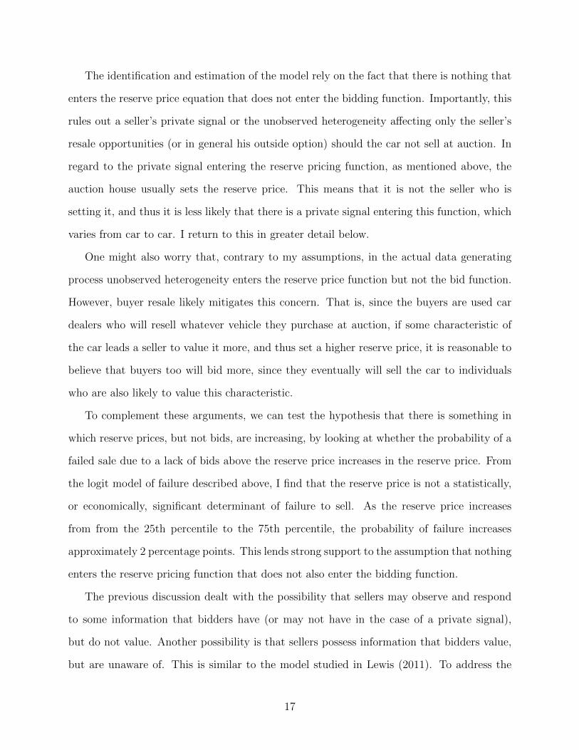
To complement these arguments, we can test the hypothesis that there is something in

which reserve prices, but not bids, are increasing, by looking at whether the probability of a

failed sale due to a lack of bids above the reserve price increases in the reserve price. From

the logit model of failure described above, I find that the reserve price is not a statistically,

or economically, significant determinant of failure to sell. As the reserve price increases

from from the 25th percentile to the 75th percentile, the probability of failure increases

approximately 2 percentage points. This lends strong support to the assumption that nothing

enters the reserve pricing function that does not also enter the bidding function.

The previous discussion dealt with the possibility that sellers may observe and respond

to some information that bidders have (or may not have in the case of a private signal),

but do not value. Another possibility is that sellers possess information that bidders value,

but are unaware of. This is similar to the model studied in Lewis (2011). To address the

17

possibility that sellers in these auctions have information that bidders would like to know,

one needs to consider how sellers behave in this informational environment. That is, how

should the possession of private information that is valuable to bidders affect seller behavior?

Cai, Riley, and Ye (2007) show that when bidders value a seller’s private information, it is

incentive compatible for sellers to use their reserve price as a signal of this information:

there is a separating equilibrium in which sellers with higher realizations of the private

information set higher reserve prices. Moreover, there is a testable implication of this model

in the data. Cai, Riley, and Ye (2007) also show that when reserve prices can be used as

signals, the optimal reserve price is increasing in the number of bidders. When the log of

reserve prices is regressed on automobile’s characteristics in specification 3 in table 2 and the

number of bidders, the effect of the number of bidders on reserve prices is small, negative and

statistically insignificant. This, along with the previous evidence that there is not a private

signal which affects reserve prices but not bids, provides support for modeling reserve prices

as functions of Z and U alone.

Another important assumption about bidders is that they are symmetric. Without this

assumption, and without data on bidder identities, we cannot recover the distribution of

bidder values using only the winning bid. The assumption of bidder symmetry is reasonable

in this context as the used car dealers in these data tend to be uniformly relatively small

and do not specialize in certain types of vehicles. However, it is possible that the sources of

bidder inventories may differ in a way that makes some bidders stronger competitors than

others at the auction. For example, if the auction house is the only source of cars for a

dealer, that dealer may wish to pay higher prices for the same vehicle than another with

multiple inventory sources would not. While there is some evidence that a few buyers tend

to buy more vehicles at the auction house than others, 75% of bidders purchase 17 or fewer

automobiles across 59 distinct auction days.

Finally, I have assumed throughout that all sellers use the same reserve pricing function

m(·). This is potentially problematic since individual sellers are the ones bringing the auto-

18

mobiles to be sold. However, the majority of the time the auction house provides guidance

on how to set the reserve price of the car (however, the data do not identify in which specific

instances this occurs). To the extent that the auction house is an “expert” on the auction

market, it then serves as a mechanism for translating car characteristics into reserve prices.

Moreover, as the analysis will bear out, reserve prices appear to move in consistent ways

across vehicles despite the fact that the identity of the sellers is changing. In general, if seller

characteristics were observed, the reserve pricing function could vary with these attributes

and thus differ across sellers.

4 Estimation

In this section I report estimates of the distribution of bidder values. As described in Section

2, I begin by specifying a flexible functional form for R = m(Z1, U). Z1 includes a car’s age

and mileage as I will condition the analysis on the make and model of each vehicle. I assume

that m(Z1, U) = g(X;α) +U , where g(·) is a known quadratic function, up to parameters α,

of covariates X that are a car’s age, mileage, age squared, mileage squared, the interaction

of age and mileage and a constant and I assume that E[UX] = 0 and E[XX ′] = 0.7

In the second stage, I consider all auctions with N potential bidders and characteristics

Z2. In practice, Z2 = Z1 when unobserved heterogeneity is ignored, and Z2 = [Z1 U ] when

it is not. To avoid repeating notation, when I condition on Z below it is understood to

stand for either Z1 or Z2 according to whether or not unobserved heterogeneity is controlled

for. Below I outline how I specify the number of potential bidders and smooth across cars

with differing characteristics. The distribution of winning bids for these auctions is related

to the distribution of values for these cars as follows. Let v(i:N) be the ith highest of N

draws from FV and denote its distribution by FV(i:N). By ignoring the auctions’ tiny bid

increments, we know that if FW |Z,N is the distribution of winning bids across auctions with

7Including other covariates, like a car’s color, or using a cubic instead of a quadratic did not materiallychange the results.

19

N potential bidders, then FW |Z,N = FV(2:N)|Z . Furthermore (see Athey and Haile (2002) and

more generally Arnold, Balakrishnan, and Nagaraja (1992)):

FV(i:N)|Z (v) = φ(FV |Z ;N) =N !

(N − i)!(i− 1)!

∫ FV |Z(v)

0

sN−i(1− s)i−1ds (2)

where φ(·) is a known and strictly monotonic function.

The estimation technique is a two step procedure. First FV(2:N)(v) must be obtained from

the distribution of winning bids, which I estimate using the non-parametric kernel estimator

for this distribution from Nadaraya (1964):

FW |Z=z(v) =

∑Tt=1 k1(

v−W t

h)k2(

z−Zt

h)∑T

t=1 k2(z−Zt

h)

(3)

where h is the bandwidth, k1 : R → R and k2 : RL → R are kernel functions, and k1 =∫ u∞ k1(s)ds. I smooth across covariates using a Gaussian kernel proportional to the standard

bandwidth suggested by Silverman (1986).

Once the distribution of winning bids is estimated, the estimate of FV |Z=z(v) is obtained

via the known inverse mapping φ(·)−1 from equation (2) above. Provided that we have a

consistent estimator of the distribution of winning bids, since φ(·) is a continuous function,

the continuous mapping theorem implies that the estimator of FV |Z2=z2(v) will be consistent.

Sufficient conditions (see, for example, Matzkin (2003)) for FW |Z=z(v) to be a consistent

estimator when Z contains an estimated covariate (i.e. Z = Z2) are that the kernel functions

in equation (3) are Lipschitz continuous, h2T√T/lnT →∞ and E|Z| <∞. These conditions

are met in estimation.

As the above discussion makes clear, the estimate of the distribution of values depends on

N . While some data sets include a natural measure of N , the set of potential bidders in these

car auctions is not obvious.8 One possibility is to assume that the number of observed bidders

8Song (2004) suggests a method for avoiding this assumption, but this requires having data on more thanone bid and being able to interpret all bids used in the estimation procedure as order statistics. Since I onlyhave data on the winning bid, I am forced to take a stand regarding the number of potential bidders in an

20

in any auction is the set of potential bidders for that auction. This is problematic if some

potential bidders do not bid. Therefore, I assume that the number of potential bidders is the

maximum of the number of bidders bidding in any one auction. To support this assumption,

I only pool across auction days if the number of bidders showing up at the auction house

is similar on these days. There is not much variation within any month, but there is some

variation across months. Therefore, I only pool across months with approximately the same

number of total unique bidders. All the results below consider months 10/2001, 11/2001,

12/2001, 1/2002, 5/2002, 7/2002, 8/2002, 9/2002 and 10/2002, across which the average

number of unique bidder is 62.6. I further restrict the set of cars to Hyundai Sonatas. To

avoid outliers, I drop all auctions with more than eight bidders, which leaves over 92% of the

auctions. I will thus assume N = 8. Table 5 presents summary statistics for this restricted

sample.

Compared to the full sample of cars summarized in table 1, cars in this restricted sample

tend to have moderately higher winning bids and mileage. Approximately the same number

of bidders submit bids for these cars. Importantly, as was the case in the full sample, in this

restricted sample there is a high degree of correlation in reserve prices and winning bids. If

we control for the (log of) reserve price in a regression of the (log of) winning bid on age,

mileage, color dummies and month dummies, the adjusted R2 jumps from 0.773 to 0.971. In

addition, the correlation in residuals from regressions of the winning bid and reserve price

on these same covariates is 0.9343, compared to 0.9835 in the raw data for this sample.

To illustrate the estimation results, figure 1 presents estimates of the distribution of val-

ues for a seven year old car with 100,000 KMs both ignoring unobserved heterogeneity and

assuming its realization of U is at the 10th, 50th and 90th percentiles for this type of car.

The solid distribution ignores unobserved heterogeneity. Clearly this increases the estimated

variance of the distribution of values. This is expected since more of the variation in bids is

attributed to variation in values. Focusing on the three distributions controlling for unob-

auction.

21

served heterogeneity, there is a clear ordering of the distributions. The value distributions

for cars with higher realizations of U maintain a first order stochastic dominance over those

with lower realizations. For example, the estimated mean [with bootstrapped 95% confi-

dence intervals based on 100 repetitions] of these distributions are, respectively, $1,919.61

[$1,904.37, $1,937.11], $2,426.20 [$2,406.88, $2,448.65] and $2,971.17 [$2,946.99, $2,999.08].

This is intuitive since whatever the econometrician is not observing, the more favorable is

this characteristic, the higher ought to be both the bids and the reserve prices.9,10

Optimal Reserve Price and Auction House Performance

Auction platforms, such as the auction house considered in this article, are often attractive to

individual sellers when it may be difficult to locate and negotiate with potential buyers. The

ability to access a centralized, formal auction environment attracting numerous potential

9To check the robustness of the estimates to my assumption regarding the number of bidders, I have alsoestimated value distributions assuming that N = 7 and N = 9. The results indicate that the estimateschange, as they must, but not by very much. Moreover, the changes are intuitive. For example, if we assumeN = 7 and estimate the distribution of values for seven year old automatic, five passenger, Hyundai Sonataswith 100,000 KMs, which are the basis for figure 1, the distributions are similar, but first order stochasticallydominated by those assuming N = 8. This is intuitive since the winning bids are interpreted to be the secondhighest value from a smaller sample of bidders, and so the distribution they are inferred to be drawn frommust contain higher values, on average. The opposite is true when it is assumed that N = 9. When it isassumed that N = 7, the means of the same value distributions are $2,168.82, $2,542.19, and $3,146.35,respectively. When it is assumed that N = 9, the means of the same value distributions are $1,871.81,$2,326.22, and $2,788.02, respectively.

10An alternative way to approach estimation is to specify functional forms for the distribution of valuesand the number of potential bidders and to estimate these distributions’ parameters via maximum likelihood.While the advantage to this approach is that it does not require specifying the number of bidders, it doesnecessitate specifying functional forms for the distribution of potential bidders as well as the distribution ofbidder values, which the current method avoids doing. Additionally, the identification of the parameters ofeach specified distribution is based purely off of functional form assumptions since the model will attempt toexplain the data (the distribution of winning bids) by a mixture of second order statistics, with weights deter-mined by the probability masses for different numbers of potential bidders. Nevertheless, I have attemptedto implement such an approach. Based on the distribution of the log of winning bids looking approximatelynormal, I assumed that FV = lognormal(Z2β, σ) and Pr[N = n] = Poisson(λ). I allow the number ofpotential bidders to range from 2 to 20 and estimate the model using maximum likelihood, integrating outover the number of potential bidders. I find that the estimated mean of the distribution of bidder valuesfor a seven year old Hyundai Sonata with 100,000 KMs is $1,758.45, $2,184.41 and $2,864.57, when therealization of unobserved heterogeneity is at its 10th, 50th and 90th percentile, respectively. The estimatedaverage number of potential bidders is 8.84. While this approach has its drawbacks, the fact that standardfunctional form choices for the distribution of values and the number of potential bidders produced estimatesof the distribution of values and a mean number of bidders that are similar to those in the benchmark caseabove lends support to the estimation approach used throughout the article.

22

buyers is one reason platforms such eBay, or well-known auction houses like Christie’s or

Sotheby’s, are so popular among individual sellers of art, wine and other miscellaneous

goods. When price discovery is important, these auctions allow a seller to avoid having to

set a (potentially uninformed) fixed price or negotiate with buyers. In this section, I evaluate

how well sellers do in capturing the value from selling their car at the auction house. I then

explore the channels through which the auction house improves an individual’s ability to sell

his automobile. There are at least three obvious ways by which a seller can benefit. The

first channel is the simultaneous competition among buyers that an auction house generates.

Related to this is a reduction in a seller’s cost of reaching buyers. The second channel is the

attraction of additional potential buyers. When these buyers must compete in an auction, as

they do at this platform, an additional bidder is worth more than any amount of negotiating

power the seller may have with the original set of bidders. Third, the auction house’s reserve

price enables the seller to retain some bargaining power with the set of bidders.

To begin, I estimate the fraction of the maximum potential value from selling their car

that sellers capture by using the auction house, assuming that they could hold the optimal

auction with the actual set of potential buyers from the auction house. It is well-known

that a seller’s optimal mechanism with a fixed set of buyers is an open outcry auction with

an optimal reserve price. However, in estimating the optimal reserve price, controlling for

unobserved heterogeneity is crucial. To see the impact of ignoring unobserved heterogeneity

on a common policy variable of interest11, I estimate how the optimal reserve price would

change based on whether the estimated distribution of values, which affects the optimal

reserve price, controls for unobserved heterogeneity. According to equation (1), the optimal

reserve price also depends on v0. As is often the case, the data provide no direct measures

for v0. Thus, I follow the literature12 and estimate the optimal reserve prices for a variety

11Reserve prices have figured centrally in the empirical auction literature as they were some of the originalpolicy variables of interest in such work as Paarsch (1997). Other examples of estimating optimal reserveprices include Mead, Schniepp, and Watson (1981), Mead, Schniepp, and Watson (1984), Paarsch (1997),Haile and Tamer (2003), Li and Perrigne (2003) and Aradillas-Lopez, Gandhi, and Quint (2013).

12A similar technique is used in Haile and Tamer (2003). As noted there, unlike the requirement inMyerson (1981) that the inverse hazard rate is strictly monotone in ρ, not U , this procedure only requires

23

of reasonable values for v0 and let these values vary with the value of the car by specifying

v0 = γR, for an assumed γ.

Table 6 presents comparisons of estimates of the optimal reserve prices controlling and

not controlling for unobserved heterogeneity for different values of γ. Let R∗C and R∗NC be

the optimal reserve prices when the distribution of values is estimated controlling and not

controlling for unobserved heterogeneity, respectively. For each value of γ, table 6 shows the

average of R∗C −R∗NC across all cars, and R∗C −R∗NC for cars with unobserved heterogeneity

within 0.5 standard deviations of the median realization of unobserved heterogeneity across

all cars. The results in table 6 are intuitive. Ignoring unobserved heterogeneity tends to

overstate the dispersion in values and this will tend to bias the optimal reserve price upward.13

Focusing on the second column, which is less subject to relatively high or low realizations

of unobserved heterogeneity than the first column, the difference in optimal reserve prices

tends to grow in v0. In general, a reserve price is more valuable to a seller the greater is

v0 since the cost of failing to sell the item is lower. This effect, combined with the upward

pressure that increased dispersion in values places on reserve prices, rationalizes the results

that the difference in optimal reserve prices tends to grow in v0.

The remaining columns in table 6 estimate the fraction of value the seller is able to

capture by selling his car at the auction house. Revenues are estimated via simulation

(using 10,000 simulations) with different reserve prices assuming that N = 8. In general,

the reserve price set by the auction house will not be the individual seller’s optimal reserve

price. This may occur for a variety of reasons including the fact that the auction house

sells multiple automobiles per day and faces at least some competition from other auction

that Π(ρ; v0, FV ) is strictly pseudo-concave on A ⊆ R which means that for all distinct a1 and a2 ∈ A, ifΠ′(a1)(a2 − a1) ≤ 0, then Π(a2)−Π(a1) < 0. See Avriel, Diewert, Schaible, and Zang (1988).

13Formally, a sufficient, but not necessary, condition for this result is that the estimated distribution ofvalues ignoring unobserved heterogeneity hazard rate dominates that controlling for unobserved heterogene-ity, provided the usual regularity condition (see Proposition 1) holds. To see this, let λC(·) and λNC(·) bethe hazard rates of the distribution of values controlling and not controlling for unobserved heterogeneity,respectively. The assumptions of hazard rate dominance gives λC(r) > λNC(r) for all r. Suppose thatr∗C = v0 + 1

λC(r∗C) . Then hazard rate dominance delivers that r∗C − 1λNC(r∗C) < v0. Regularity assures that for

a value r∗NC such that r∗NC = v0 + 1λNC(r∗NC) , it must be that r∗NC > r∗C .

24

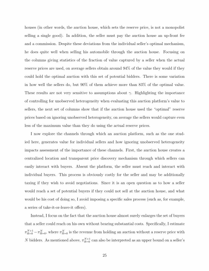
houses (in other words, the auction house, which sets the reserve price, is not a monopolist

selling a single good). In addition, the seller must pay the auction house an up-front fee

and a commission. Despite these deviations from the individual seller’s optimal mechanism,

he does quite well when selling his automobile through the auction house. Focusing on

the columns giving statistics of the fraction of value captured by a seller when the actual

reserve prices are used, on average sellers obtain around 94% of the value they would if they

could hold the optimal auction with this set of potential bidders. There is some variation

in how well the sellers do, but 90% of them achieve more than 83% of the optimal value.

These results are not very sensitive to assumptions about γ. Highlighting the importance

of controlling for unobserved heterogeneity when evaluating this auction platform’s value to

sellers, the next set of columns show that if the auction house used the “optimal” reserve

prices based on ignoring unobserved heterogeneity, on average the sellers would capture even

less of the maximum value than they do using the actual reserve prices.

I now explore the channels through which an auction platform, such as the one stud-

ied here, generates value for individual sellers and how ignoring unobserved heterogeneity

impacts assessment of the importance of these channels. First, the auction house creates a

centralized location and transparent price discovery mechanism through which sellers can

easily interact with buyers. Absent the platform, the seller must reach and interact with

individual buyers. This process is obviously costly for the seller and may be additionally

taxing if they wish to avoid negotiations. Since it is an open question as to how a seller

would reach a set of potential buyers if they could not sell at the auction house, and what

would be his cost of doing so, I avoid imposing a specific sales process (such as, for example,

a series of take-it-or-leave-it offers).

Instead, I focus on the fact that the auction house almost surely enlarges the set of buyers

that a seller could reach on his own without bearing substantial costs. Specifically, I estimate

πN+1R=0 −πNR=0, where πNR=0 is the revenue from holding an auction without a reserve price with

N bidders. As mentioned above, πN+1R=0 can also be interpreted as an upper bound on a seller’s

25

revenue from negotiating with N bidders on his own given that Bulow and Klemperer (1996)

show that no amount of bargaining power with N buyers is worth as much as adding one

more buyer and holding an auction with no reserve price.

Finally, in practice sellers can set reserve prices at the auction house. This transfers some

amount of the bargaining power, which the last channel assumed away, back to sellers. So

the third, and final, channel through which sellers benefit comes from the seller setting a

reserve price: πN+1R=R∗ − π

N+1R=0 .

Table 7 shows a breakdown of the importance of these channels, both when unobserved

heterogeneity is controlled for and when it is not, for various number of bidders, assuming

here that γ = 0. The first row in each panel displays the average increase in seller revenue,

based on 10,000 simulations, when an auction with N+1 bidders and an optimal reserve price

is used as compared to when the seller holds an auction with N buyers and no reserve price.

The next rows in each panel of the table display the fraction of this difference attributable

to adding another bidder and setting an optimal reserve price, respectively. Clearly the

advantage of the auction with an extra bidder and an optimal reserve price decreases in the

number of buyers, as should be expected. However, the fraction for which each channel is

responsible is not constant. As N increases, the first channel, the simultaneous competition

created by the auction house, becomes relatively more important, while the third, the ability

to set an optimal reserve price, becomes relatively inconsequential. Across N , the ability of

the auction house to attract additional bidders is valued by sellers, and by a much greater

amount than were they able to set an optimal reserve price. For example, when there are

five bidders, the value of adding an additional bidder is worth approximately 17.5 times on

average as much to the seller as being able to set an optimal reserve price with the original

set. In other words, the relative effect of adding another bidder, as compared to setting

an optimal reserve price, shows that the classic theoretical result of Bulow and Klemperer

(1996) is economically significant in a relevant empirical setting.

The second panel of table 7 shows the importance of each channel when unobserved

26

heterogeneity is ignored. The main difference centers on the importance of reserve prices.

Consistent with the findings in table 6, when unobserved heterogeneity is ignored, reserve

prices have a greater impact on seller revenues. Moreover, the relative importance of adding

another bidder as compared to setting a reserve price is also understated. Now, when there

are five bidders, the ability to add another bidder, even if no reserve price is set, is worth only

4.6 times as much as the ability to set an optimal reserve with the original set of bidders.

5 Conclusion

The existing empirical auction literature has improved our understanding of how a variety

of auctions operate in practice and has answered questions of practical importance such as

revenue maximizing design, the detection of collusion and the estimation of firm markups.

Much of this literature, however, ignores unobserved heterogeneity. While several recent

attempts have been made to address this empirical issue, the current article proposes a

new methodology that relies on using information from the behavior of individuals other

than bidders (who are the only auction participants currently used in efforts to control for

unobserved heterogeneity), namely sellers, to help control for what the researcher does not

observe in the data.

Oftentimes such seller behavior is available. The solution relies on a strict monotonicity

assumption in the seller behavior, which is intuitively plausible and, while not required in the

model, generally is the outcome of optimal seller behavior. Evidence from used car auctions

clearly shows the importance of controlling for unobserved heterogeneity. Estimates of the

optimal reserve price, which is a key tool of mechanism design and a frequently analyzed

object in the empirical auction literature, will depend on whether unobserved heterogeneity

is controlled for.

Given that the data come from individuals using an auction platform to sell their vehicles,

a natural question is to what extent sellers are able to capture the value from selling their

27

automobile in this environment. On the one hand, the auction house will not generally set

the same reserve price that the individual would set if he could hold an optimal auction. On

the other hand, sellers clearly benefit from the auction house’s formal bidding environment,

which allows them to avoid the pains of negotiating, and gives them access to a large set

of buyers, who may be costly to interact with absent the platform. One way to gauge the

performance of the platform from a seller’s perspective is to estimate a seller’s value of the

platform’s auction and compare this to the seller’s value of holding the optimal auction with

the same set of bidders. By this benchmark, the auction platform allows sellers to capture

a large fraction, on average over 90%, of this maximum potential value. However, this likely

understates the benefit of the auction platform to individual sellers since it is costly for

sellers to locate and interact with the same set of buyers on their own. To support the claim

that access to more bidders particularly benefits sellers, I show that increasing the number

of bidders substantially improves seller revenues even if they cannot set any reserve price. I

also show that the benefit of an additional bidder relative to setting an optimal reserve price

depends on whether unobserved heterogeneity is controlled for, and if it is not, I find that

the relative gain will be understated.

One path for future work is to incorporate multi-dimensional unobserved heterogeneity.

I speculate that the identification result above can be generalized to this setting. Suppose,

for example, that the signal U ∈ RL1, L1 > 1. One could require that there exist as many

policy variables (denoted by what is now a vector R) as there are dimensions of U , L1, and

that for each component of R ∈ RL2, L2 ≥ L1, say Rl, there exist functions Rl = ml(Z,Ul)

which are monotonic in Ul. Then, if we allow the bids to depend on the entire vector U ,

we can simply perform the “first part” of the above proof L1 times to each of the functions

m(·) in order to uncover all of the realizations of unobserved heterogeneity, but this remains

to be shown. One setting that is potentially appropriate for such a model is eBay, where

sellers can choose not only reserve prices, but also auction length, whether or not to display

pictures of the item, whether or not to have the object insured, shipping charges, etc.

28

References

Aradillas-Lopez, A., A. Gandhi, and D. Quint (2013): “Identification and Inference

in Ascending Auctions with Correlated Private Values,” Econometrica, 81(2), 489–534.

Arnold, B., N. Balakrishnan, and H. N. Nagaraja (1992): A First Course in Order

Statistics. Wiley & Sons, Inc., New York, NY.

Asker, J. (2010): “A Study of the Internal Organization of a Bidding Cartel,” American

Economic Review, 100(3), 724–762.

Athey, S., P. Cramton, and A. Ingraham (2003): “Upset Pricing in Auction Markets:

An Overview,” White Paper, Market Design, Inc., on behalf of British Columbia Ministry

of Forests.

Athey, S., and P. Haile (2006): Empirical Models of Auctions, vol. 2 of Advances in Eco-

nomics and Econometrics, Theory and Applications: Ninth World Congress. Cambridge

University Press.

Athey, S., and P. A. Haile (2002): “Identification of Standard Auction Models,” Econo-

metrica, 70(6), 2107–2140.

Athey, S., J. Levin, and E. Seira (2011): “Comparing Open and Sealed Bid Auctions:

Theory and Evidence from Timber Auctions,” Quarterly Journal of Economics, 126(1),

207–257.

Avriel, M., W. E. Diewert, S. Schaible, and I. Zang (1988): Generalized Concavity.

Plenum, New York, NY.

Bagnoli, M., and T. Bergstrom (2005): “Log-Concave Probability and its Applica-

tions,” Economic Theory, 26(2), 445–469.

Bulow, J., and P. Klemperer (1996): “Auctions Versus Negotiations,” American Eco-

nomic Review, 86(1), 180–194.

29

Cai, H., J. Riley, and L. Ye (2007): “Reserve Price Signaling,” Journal of Economic

Theory, 135, 253–268.

Cassady, R. (1967): Auctions and Auctioneering. University of California Press, Berkeley,

CA.

Decarolis, F. (2009): “When the Highest Bidder Loses the Auction: Theory and Evidence

from Public Procurement,” Working Paper.

Einav, L., and A. Nevo (2007): Empirical Models of Imperfect Competition: A Discus-

sion Advances in Economics and Econometrics: Theory and Applications: Ninth World

Congress.

Ewerhart, C. (2011): “Optimal Design and ρ-Concavity,” Working Paper.

Guerre, E., I. Perrigne, and Q. Vuong (2009): “Nonparametric Identification of

Risk Aversion in First-Price Auctions Under Exclusion Restrictions,” Econometrica, 77(4),

1193–1228.

Haile, P., H. Hong, and M. Shum (2006): “Nonparametric Tests for Common Values

In First-Price Sealed-Bid Auctions,” Working Paper.

Haile, P. A., and E. Tamer (2003): “Inference with an Incomplete Model of English

Auctions,” Journal of Political Economy, 111(1), 1–51.

Hu, Y., D. McAdams, and M. Shum (2013): “Identification of First-Price Auction Models

with Non-Separable Unobserved Heterogeneity,” Journal of Econometrics, 174(2), 186–

193.

Klemperer, P. (2002): “What Really Matters in Auction Design,” Journal of Economic

Perspectives, 16(1), 169–189.

Kontos, T. (2006): “Vehicle Remarketing and the Dealer,” Industry report, ADESA, Inc.

30

Krasnokutskaya, E. (2011): “Identification and Estimation in Highway Procurement

Auctions Under Unobserved Auction Heterogeneity,” Review of Economic Studies, 78(1),

293–327.

Laffont, J.-J., H. Ossard, and Q. Vuong (1995): “Econometrics of First Price Auc-

tions,” Econometrica, 63(4), 953–980.

Lewis, G. (2011): “Asymmetric Information, Adverse Selection and Seller Disclosure: The

Case of eBay Motors,” American Economic Review, 101(4), 1535–1546.

Li, T., and I. Perrigne (2003): “Timber Sale Auctions with Random Reserve Prices,”

Review of Economics and Statistics, 85(1), 189–200.

Li, T., I. Perrigne, and Q. Vuong (2000): “Conditionally Independent Private Infor-

mation in OCS Wildcat Auctions,” Journal of Econometrics, 98(1), 129–161.

Li, T., and Q. Vuong (1998): “Nonparametric Estimation of the Measurement Error

Model Using Multiple Indicators,” Journal of Multivariate Analysis, 65(2), 139–165.

Matzkin, R. (2003): “Nonparametric Estimation of Nonadditive Random Functions,”

Econometrica, 71(5), 1339–1375.

Mead, W. J., M. Schniepp, and R. Watson (1981): “The Effectiveness of Compe-

tition and Appraisals in the Auction Markets for National Forest Timber in the Pacific

Northwest,” Washington, DC: U.S. Department of Agriculture, Forest Service.

(1984): “Competitive Bidding for U.S. Forest Service Timber in the Pacific North-

west 1963-83,” Washington, DC: U.S. Department of Agriculture, Forest Service.

Milgrom, P., and R. Weber (1982): “A Theory of Auctions and Competitive Bidding,”

Econometrica, 50(5), 1089–1122.

Myerson, R. (1981): “Optimal Auction Design,” Mathematics of Operations Research,

6(1), 58–73.

31

Nadaraya, E. (1964): “Some New Estimates for Distribution Functions,” Theory of Prob-

ability and Its Applications, 15, 497–500.

Olley, S., and A. Pakes (1996): “The Dynamics of Productivity in the Telecommunica-

tions Equipment Industry,” Econometrica, 65(6), 1263–1297.

Paarsch, H. J. (1997): “Deriving an Estimate of the Optimal Reserve Price: An Applica-

tion to British Columbia Timber Sales,” Journal of Econometrics, 78, 333–357.

Pakes, A. (2008): “Theory and Empirical Work on Imperfectly Competitive Markets,”

Working Paper.

Riley, J., and W. Samuelson (1981): “Optimal Auctions,” American Economic Review,

71, 58–73.

Roberts, J., and A. Sweeting (forthcoming): “When Should Sellers Use Auctions?,”

American Economic Review.

Silverman, B. (1986): Density Estimation for Statistics and Data Analysis. Chapman Hall,

London.

Song, U. (2004): “Nonparametric Estimation of an eBay Auction Model with an Unknown

Number of Bidders,” Working Paper.

Taylor, P. (2007): “NADA Data 2007,” Annual Report, National Automobile Dealers

Association.

32

Tables and Figures

Variable Mean Std. Dev. 25th-tile Median 75th-tileWINNING BID (in $) 3661.83 2889.37 1450.00 3260.00 5150.00RESERVE PRICE (in $) 3361.26 2842.75 1200.00 3000.00 4800.00WINNING BID/RESERVE PRICE 1.20 0.44 1.03 1.09 1.20WINNING BID - RESERVE PRICE 300.57 294.89 90.00 240.00 450.00NUMBER OF UNIQUE BIDDERS 5.37 2.40 3.00 5.00 7.00AGE (in months) 73.60 28.79 56.00 76.00 95.00MILEAGE (in 100,000 km’s) 0.96 0.48 0.64 0.95 1.25

Table 1: Auction summary statistics. There are 4,943 observations of each variable andthe time period is 10/10/2001-11/27/2002. During the period of study there were 28,334passenger cars auctioned. The types of car auctioned were sedans, hatchbacks, jeeps, smallminivans, minibuses, small trucks and motorbikes. Unlike the U.S., SUVs were not prevalentin South Korea at this time. In an effort to maintain a homogenous data set, the samplesummarized in this table consists of 5 passenger sedans with automatic transmissions thathad been previously owned for “regular” individual purposes, as opposed to being part ofgovernment or rental company fleets. All variables are measured at the time of auction. HereAGE is the number of months since the car was originally manufactured and MILEAGE isthe reading on the odometer in 100,000s of kilometers.

33

(1)

(2)

(3)

(4)

(5)

(6)

(7)

AG

E-0

.026∗∗∗

-0.0

26∗∗∗

-0.0

23∗∗∗

-0.0

23∗∗∗

-0.0

23∗∗∗

-0.0

05∗∗∗

(0.0003)

(0.0003)

(0.0003)

(0.0003)

(0.0003)

(0.0002)

MIL

EA

GE

0.11

4∗∗∗

0.12

6∗∗∗

-0.0

32∗∗∗

-0.0

37∗∗

-0.0

30∗

-0.0

09(0.021)

(0.02)

(0.012)

(0.018)

(0.017)

(0.008)

NU

MB

ER

OF

BID

DE

RS

0.03

4∗∗∗

0.02

4∗∗∗

0.02

2∗∗∗

0.02

2∗∗∗

0.02

7∗∗∗

(0.003)

(0.002)

(0.002)

(0.002)

(0.0008)

LO

GR

ESE

RV

EP

RIC

E0.

711∗∗∗

0.87

1∗∗∗

(0.005)

(0.002)

MA

KE

DU

MM

IES

NO

NO

YE

SY

ES

YE

SY

ES

NO

MO

DE

LD

UM

MIE

SN

ON

OY

ES

YE

SY

ES

YE

SN

O

MA

KE

/MO

DE

LD

UM

MIE

SN

ON

OY

ES

YE

SY

ES

YE

SN

O

MA

KE

/MO

DE

LD

UM

MIE

S×

MIL

EA

GE

DU

MM

IES

NO

NO

NO

YE

SY

ES

YE

SN

O

CO

LO

RD

UM

MIE

SN

ON

ON

ON

OY

ES

YE

SN

O

MO

NT

HD

UM

MIE

SN

ON

ON

ON

OY

ES

YE

SN

OT

4,94

34,

943

4,94

34,

943

4,94

34,

943

4,94

3R

20.

623

0.63

30.

889

0.89

60.

903

0.97

90.

966

Tab

le2:

Win

nin

gbid

det

erm

inan

ts.

OL

SR

egre

ssio

ns

wher

eth

edep

enden

tva

riab

leis

the

log

ofth

ew

innin

gbid

inea

chau

ctio

n.

The

tim

ep

erio

dis

from

10/1

0/20

01-1

1/27

/200

2.M

AK

E/M

OD

EL

DU

MM

IES×

MIL

EA

GE

DU

MM

IES

mea

ns

that

indic

ator

sfo

rth

em

ake

and

model

ofth

eve

hic

lear

ein

tera

cted

wit

hin

dic

ator

sfo

rw

het

her

the

car’

sm

ilea

geis

bet

wee

nth

e25

than

d75

thp

erce

nti

leof

milea

ge(0

.64

and

1.25

,re

spec

tive

ly),

orgr

eate

rth

anth

e75

thp

erce

nti

leof

milea

ge.

Inte

ract

ing

the

mak

ean

dm

odel

dum

mie

sw

ith

afiner

par

sing

ofm

ilea

gedoes

not

mat

eria

lly

affec

tan

yof

the

resu

lts.∗ ,∗∗

,∗∗∗

imply

sign

ifica

nce

atth

e10

%,

5%an

d1%

leve

l,re

spec

tive

ly.

34

(1)

(2)

(3)

(4)

(5)

(6)

AG

E-0

.026∗∗∗

-0.0

05∗∗∗

-0.0

26∗∗∗

-0.0

05∗∗∗

(0.0007)

(0.0005)

(0.0007)

(0.0005)

MIL

EA

GE

-0.0

240.

013

-0.0

240.

013

(0.027)

(0.013)

(0.027)

(0.013)

NU

MB

ER

OF

BID

DE

RS

0.02

8∗∗∗

0.03

1∗∗∗

0.02

8∗∗∗

0.03

1∗∗∗

(0.004)

(0.002)

(0.004)

(0.002)

LO

GR

ESE

RV

EP

RIC

E0.

708∗∗∗

0.88

7∗∗∗

0.70

8∗∗∗

0.89

1∗∗∗

(0.012)

(0.005)

(0.012)

(0.006)

MA

KE

DU

MM

IES

YE

SY

ES

NO

YE

SY

ES

NO

MO

DE

LD

UM

MIE

SY

ES

YE

SN

OY

ES

YE

SN

O

MA

KE

/MO

DE

LD

UM

MIE

SY

ES

YE

SN

OY

ES

YE

SN

O

MA

KE

/MO

DE

LD

UM

MIE

S×

MIL

EA

GE

DU

MM

IES

YE

SY

ES

NO

YE

SY

ES

NO

CO

LO

RD

UM

MIE

SY

ES

YE

SN

OY

ES

YE

SN

O

MO

NT

HD

UM

MIE

SY

ES

YE

SN

OY

ES

YE

SN

O

T1,

117

1,11

71,

117

1,11

71,

117

1,11

7R

20.

910

0.98

00.

959

0.91

00.

980

0.95

4D

epen

den

tV

aria

ble

Max

Bid

Max

Bid

Max

Bid

Mea

nB

idM

ean

Bid

Mea

nB

id

Tab

le3:

Hig

hes

tbid

and

mea

nbid

det

erm

inan

ts.

OL

SR

egre

ssio

ns

ofth

ehig

hes

tbid

and

mea

nbid

subm

itte

din

auct

ions

bet

wee

n10

/10/

2001

-12/

27/2

001.

MA

KE

/MO

DE

LD

UM

MIE

S×

MIL

EA

GE

DU

MM

IES

mea

ns

that

indic

ator

sfo

rth

em

ake

and

model

ofth

eve

hic

lear

ein

tera

cted

wit

hin

dic

ator

sfo

rw

het

her

the

car’

sm

ilea

geis

bet

wee

nth

e25

than

d75

thp

erce

nti

leof

milea

ge(0

.64

and

1.25

,re

spec

tive

ly),

orgr

eate

rth

anth

e75

thp

erce

nti

leof

milea

ge.

Inte

ract

ing

the

mak

ean

dm

odel

dum

mie

sw

ith

afiner

par

sing

ofm

ilea

gedoes

not

mat

eria

lly

affec

tan

yof

the

resu

lts.∗ ,∗∗

,∗∗∗

imply

sign

ifica

nce

atth

e10

%,

5%an

d1%

leve

l,re

spec

tive

ly.

35

(1) (2) (3) (4)AGE 0.008∗ 0.005 -0.002 0.005

(0.005) (0.005) (0.006) (0.01)

MILEAGE -0.911∗∗∗ -0.859∗∗∗ -0.854∗∗∗ -0.841∗∗

(0.311) (0.322) (0.326) (0.328)

LOG RESERVE PRICE 0.232(0.263)

MAKE DUMMIES NO YES YES YES

MODEL DUMMIES NO YES YES YES

COLOR DUMMIES NO NO YES YES

MONTH DUMMIES NO NO YES YES

T 1,117 1,089 1,089 1,089Pseudo R2 0.0133 0.0348 0.0671 0.0682

Table 4: Failure to sell determinants. Logit model of failure to sell for automobiles auctionedbetween 10/10/2001-12/27/2001. 107 out of 1,117 cars failed to sell. Coefficient estimatesreported. ∗, ∗∗, ∗∗∗ imply significance at the 10%, 5% and 1% level, respectively.

Variable Mean Std. Dev. 25th-tile Median 75th-tileWINNING BID (in $) 3574.38 2244.73 2410.00 3230.00 4670.00RESERVE PRICE (in $) 3320.22 2227.41 2000.00 3000.00 4400.00WINNING BID/RESERVE PRICE 1.16 0.34 1.02 1.07 1.17WINNING BID - RESERVE PRICE 254.16 239.72 60.00 180.00 390.00NUMBER OF UNIQUE BIDS 4.83 1.89 3.00 5.00 6.00AGE (in months) 84.10 23.71 69.00 86.50 101.00MILEAGE (in 100,000 km’s) 1.13 0.46 0.85 1.10 1.41

Table 5: Auction summary statistics for five passenger Hyundai Sonatas with automatictransmissions that sold during the months cited in the text. There are 454 observations ofeach variable. All variables are measured at the time of auction. Here AGE is the number ofmonths since the car was originally manufactured, MILEAGE is the reading on the odometerin 100,000s of kilometers.

36

% of Value Captured withActual Reserves Sub-Optimal Reserves

Overall Median Percentiles Percentilesγ R∗C −R∗NC R∗C −R∗NC Mean 10th 50th 90th Mean 10th 50th 90th

0.00 $221.57 $77.21 88.42% 83.69% 89.18% 93.08% 85.53% 77.37% 94.08% 94.70%(25.36) (24.89) (0.19) (0.33) (0.18) (0.14) (0.13) (0.17) (0.03) (0.04)

0.25 258.52 90.20 90.66 86.69 91.69 93.53 86.58 74.62 94.10 94.70(23.16) (25.52) (0.18) (0.38) (0.13) (0.05) (0.11) (0.13) (0.03) (0.03)

0.50 239.72 98.45 92.23 86.98 93.69 94.25 87.60 74.05 94.05 94.70(21.35) (21.01) (0.20) (0.64) (0.04) (0.03) (0.08) (0.11) (0.03) (0.02)

0.75 236.03 123.57 91.81 85.84 93.45 94.51 88.93 80.42 94.04 94.71(21.79) (22.12) (0.20) (0.76) (0.07) (0.04) (0.07) (0.08) (0.03) (0.02)

Table 6: Comparisons of the optimal reserve prices when unobserved heterogeneity is con-trolled for and when it is not. γ is the assumed multiple to infer v0: γR =v0, where R is theobserved reserve price. The first column shows the average of the difference in the optimalreserve price ignoring unobserved heterogeneity and the optimal reserve price controlling forunobserved heterogeneity. The second column shows this average difference for cars withunobserved heterogeneity within 0.5 standard deviations of the median realization of unob-served heterogeneity across all cars. The remaining set of columns show statistics of thefraction of value captured by a seller when the actual or “optimal” reserve price ignoringunobserved heterogeneity is used. Standard errors, which for percentage estimates are inpercentage points, are based on 100 bootstrapped repetitions.

37

N 2 3 4 5 6 7

Controlling for Unobserved Heterogeneity

πN+1R=R∗ − πNR=0 $725.94 $435.5 $307.89 $233.09 $189.07 $160.59

(14.95) (8.98) (6.56) (5.13) (4.23) (3.49)

πN+1R=0−π

NR=0

πN+1R=R∗−π

NR=0

87.71% 91.91% 94.49% 96.31% 97.31% 97.97%

(0.41) (0.39) (0.34) (0.31) (0.31) (0.34)

πN+1R=R∗−π

N+1R=0

πN+1R=R∗−π

NR=0

12.29% 8.09% 5.51% 3.69% 2.69% 2.03%

(0.41) (0.39) (0.33) (0.30) (0.31) (0.34)

Not Controlling for Unobserved Heterogeneity

πN+1R=R∗ − πNR=0 $871.61 $578.62 $426.34 $333.26 $276.46 $229.27

(13.02) (7.97) (6.38) (5.33) (4.74) (4.03)

πN+1R=0−π

NR=0

πN+1R=R∗−π

NR=0

75.38% 79.11% 81.89% 83.68% 85.43% 86.46%

(0.92) (1.06) (1.15) (1.26) (1.28) (1.35)

πN+1R=R∗−π

N+1R=0

πN+1R=R∗−π

NR=0

24.62% 20.89% 18.11% 16.32% 14.57% 13.54%

(0.92) (1.07) (1.15) (1.25) (1.28) (1.36)

Table 7: Channels by which sellers benefit from the auction. The table shows a breakdownof a seller’s value from auctioning a car at the auction house. The revenues from holding anauction without a reserve price with the same set of buyers is πNR=0, and with an optimalreserve price is πNR=R∗ . Standard errors, which for percentage estimates are in percentagepoints, are based on 100 bootstrapped repetitions.

38

6 6.5 7 7.5 8 8.5 90

0.1

0.2

0.3

0.4

0.5

0.6

0.7

0.8

0.9

1

Bidder Values (in logs)

All Cars10th Percentile50th Percentile90th Percentile

Figure 1: Estimated value distributions, not controlling and controlling for unobserved het-erogeneity. Seven year old automatic, five passenger, Hyundai Sonatas with 100,000 KMs.The solid distribution is the estimated distribution of values ignoring unobserved hetero-geneity. The other four distributions control for unobserved heterogeneity at the givenpercentiles.

39

A Monte Carlo Study

In this section I provide a small simulation study of the non-parametric two step estimation

procedure. I generate reserve price and bidding data for T auctions and then repeat S times.

For the reserve price, I set R = m(Z0, Z1, U) = Z1(γ0Z0 +γ1Z1) +U , where (i) Z0 = zH0 with

probability p and Z0 = zL0 with probability 1− p, (ii) Z1 ∼ N(µHZ1, σZ1) when Z0 = zH0 and

Z1 ∼ N(µLZ1, σZ1) when Z0 = zL0 and (iii) U ∼ N(µHU , σU) when Z0 = zH0 and U ∼ N(µLU , σU)

when Z0 = zL0 . Given this specification for m(·), reserve prices are strictly increasing in

U and u = m(z0, 0, u) for all z0 and u. In addition, for this data generating process, U is

independent of Z1 conditional on Z0. For each auction t = 1, ..., T , I simulate an English

button auction by setting Nt = 4, drawing values such that Vt ∼ N(α0 + α1Ut, σV ) and

set the winning bid Wt equal to the second highest value. Given this specification, bids are

stochastically increasing in the realization of unobserved heterogeneity.

For each auction t, I assume that I only observe {Rt, Z0t, Z1t,Wt}. I experiment with

T = 250 and T = 500. For both cases, S = 100, p = 0.5, zL0 = −1, zL0 = 1, µHZ1= −2.5,

µHZ1= 2.5, σZ1 = 1, µLU = −4.5, µHU = 4.5, σU = 2.5, γ0 = 1, γ1 = 2, α0 = 100, α1 = 1 and

σV = 5. The results for estimates of m(·) and FU appear in table 8.

To investigate the performance of the estimator of the distribution of values, I consider

estimating the case where U = 0. I do this based on the first step estimates as well as

assuming that I observe the realizations of U for each auction, which generally is infeasible.

These cases are referred to as the “No Information” (NI) and “Full Information” (FI) cases,

respectively. In general, the NI case compares favorably to the generally infeasible full

information case. Additionally, increasing the sample size from 250 to 500 improves the

quality of the estimates.

40

T = 250 T = 500|Bias| Variance MSE |Bias| Variance MSE

m 0.4669 8.2817 8.6183 0.0502 5.5486 5.6057FU 0.0168 0.0150 0.0282 0.0031 0.0107 0.0223FV |U=0,“NI” 0.0225 0.0031 0.0078 0.0122 0.0022 0.0050FV |U=0,“FI” 0.0120 0.0002 0.0029 0.0105 0.0001 0.0020

Table 8: Simulation results. S = 100, p = 0.5, zL0 = −1, zL0 = 1, µHZ1= −2.5, µHZ1

= 2.5,σZ1 = 1, µLU = −4.5, µHU = 4.5, σU = 2.5, γ0 = 1, γ1 = 2, α0 = 100, α1 = 1 and σV = 5. Thesecond to last row presents estimates of the distribution of values assuming U = 0 based onthe first stage estimates. The last row assumes that the actual realizations of Ut are observedwhen estimating the distribution of values conditional on U = 0.

B Proofs

Proposition 1

Proof. Affiliation between V and U with joint density f provides that for all v1 < v2 and

u1 < u2:

f(v1, u2)f(v2, u1) < f(v1, u1)f(v2, u2)

Rearranging and making use of the corresponding conditional distributions:

f(v2|u1)f(u1)

f(v1|u1)f(u1)<f(v2|u2)f(u2)

f(v1|u2)f(u2)

and therefore by integrating with respect to v2 yields:

1− F (v1|u1)f(v1|u1)

<1− F (v1|u2)f(v1|u2)

Therefore, if r∗k is the solution when U = uk, k = 1, 2, we have1−F (r∗1 |u1)f(r∗1 |u1)

<1−F (r∗1 |u2)f(r∗1 |u2)

. Since

ψ(t, U) is increasing in t for all U , it must be that r∗1 < r∗2.

Q.E.D.

41

Proposition 2

Proof. Beginning with reserve prices, we can identify the conditional distribution of un-

observed heterogeneity as follows: FR|(Z0,Z1)=(z0,z1)(u) = Pr[R < u|(Z0, Z1) = (z0, z1)] =

Pr[m(Z0, Z1, U) < u|(Z0, Z1) = (z0, z1)] = Pr[U < u|(Z0, Z1) = (z0, z1)] = Pr[U < u|Z0 =

z0] = FU |Z0=z0(u), where the third equality comes from the normalization of m in assump-

tion (i), and the fourth comes from the conditional independence assumption (ii). Also,

we note that: FU |Z0=z0(u) = Pr[U < u|Z0 = z0] = Pr[U < u|(Z0, Z1) = (z0, z1)] =

Pr[m(Z0, Z1, U) < m(z0, z1, u)|(Z0, Z1) = (z0, z1)] = Pr[R < m(z0, z1, u)|(Z0, Z1) = (z0, z1)] =

FR|(Z0,Z1)=(z0,z1)(m(z0, z1, u)), where the second equality again uses independence and the

third uses the monotonicity of m(·, U). Therefore, the function m is identified since:

m(z0, z1, u) = F−1R|(Z0,Z1)=(z0,z1)(FR|(Z0,Z1)=(z0,z1)(u))

Now, with data on reserve prices, R, and item characteristics Z, due to the strict mono-

tonicity of m(·, U), for each (R,Z) pair there will be a unique realization of U satisfying

R = m(Z,U).

Let W0 = [Z,U ]. Using only transaction prices, we can identify F (V |W0) in a first price

and second price auction using the arguments of Theorems 6 and 1, respectively, in Athey

and Haile (2002). Q.E.D.

42