unscented kalman filter with gaussian process … kalman filter with gaussian process degradation...

Unscented Kalman Filter with Gaussian Process Degradation Modelfor Bearing Fault Prognosis

Christoph Anger B.Sc.1, Dipl.-Ing. Robert Schrader1, and Prof. Dr.-Ing. Uwe Klingauf1

1 Institute of Flight Systems and Automatic Control, Darmstadt, 64287, [email protected]

[email protected]@fsr.tu-darmstadt.de

ABSTRACT

The degradation of rolling-element bearings is mainlystochastic due to unforeseeable influences like short termoverstraining, which hampers the prediction of the remain-ing useful lifetime. This stochastic behaviour is hardly de-scribable with parametric degradation models, as it has beendone in the past. Therefore, the two prognostic concepts pre-sented and examined in this paper introduce a nonparametricapproach by the application of a dynamic Gaussian Process(GP). The GP offers the opportunity to reproduce a damagecourse according to a set of training data and thereby also esti-mates the uncertainties of this approach by means of the GP’scovariance. The training data is generated by a stochasticdegradation model that simulates the aforementioned highlystochastic degradation of a bearing fault. For prediction andstate estimation of the feature, the trained dynamic GP iscombined with the Unscented Kalman Filter (UKF) and eval-uated in the context of a case study. Since this prognostic ap-proach has shown drawbacks during the evaluation, a multi-ple model approach based on GP-UKF is introduced and eval-uated. It is shown that this combination offers an increasedprognostic performance for bearing fault prediction.

1. INTRODUCTION

Forecasting the remaining useful lifetime (RUL) of line-replaceable units (LRUs) with a high accuracy is one of themain issues in aviation to avoid unnecessary maintenance cy-cles and, therefore, to reduce aircraft life cycle costs. Onecomponent of those LRUs can be rolling-element bearings,whose RUL is of great interest and are therefore in the centreof this enquiry.Rolling-element bearings ensure the functionality of rotatingassembly parts in case of varying loading and frequency. Dur-ing their life cycle, bearings degrade in two different ways

Dipl.-Ing. Robert Schrader et.al. This is an open-access article distributedunder the terms of the Creative Commons Attribution 3.0 United States Li-cense, which permits unrestricted use, distribution, and reproduction in anymedium, provided the original author and source are credited.

according to the amount, duration and the nature of loadingand other influences. Those are e.g. contaminants or con-structive incertitudes that can affect the tribological systemof a bearing. Overstraining and solid friction caused by ahigh cyclic stress and a lack of lubricant, respectively, leadsto a rapid degradation of the bearing, as in case of calculatedstrains like wear and tear or fatigue, the course of damage in-creases continuously. A degradation process of a real bearingresults from both kinds of strains and, therefore, has a strongstochastic character (Sturm, 1986).To simulate this behaviour, several approaches of degrada-tion models (DMs) have been developed in the past. Mostof them base on the Paris-Erdogan law that describes a rela-tion between crack growth rate and effective stresses in theexamined material. By adjusting this law to existing test re-sults of real bearings, several enhancements were formulatedand evaluated, as Choi et al. did in (Choi & Liu, 2006b)and (Choi & Liu, 2006a), respectively. Other DMs are basedon the Lundberg-Palmgren model that describes the correla-tion between the probability of survival and among others themaximum shearing stress. Yu et al. refined this approach byadding a more precise geometrical description of the contactsurface in (Yu & Harris, 2001).All aforementioned models describe the degradation to de-pend on the application of external load difference, as a non-loaded bearing would not degrade at all. In reality, the degra-dation is also a function of the current degradation, since de-tached particles can lead to solid friction. The DM in thispaper that is applied to generate reliable degradation coursesconsiders both the degradation rate due to loading and due tothe state of degradation itself.Most of these DMs are used as prognostic models (PMs) incombination with state estimation. Usually particle filtersbased on the aforementioned Paris-Erdogan model are imple-mented, as done in (Orchard & Vachtsevanos, 2009). Otherprognostic concepts are based on the Archard wear equation.Daigle et al. presented a model-based prognostic approach byestimating the RUL of a pneumatic valve with a fixed-lag par-

1

European Conference of the Prognostics and Health Management Society, 2012

ticle filter (Daigle & Goebel, 2010). The appropriated modelrelates the current degradation to the wear of material basedon the Archard equation.Besides a DM that accounts for the current degradation state,Orsagh et al. presented a prognosis approach of a rolling-element bearing (Orsagh, Sheldon, & Klenke, 2003). Bymeasuring several features like e.g. the oil debris of the bear-ing or the vibration signal, they predicted the RUL dependingon the measured fused features by correlation with the currentstate of degradation. The RUL was then forecast according tothe applied PM.The prognostic concept at hand attempts another approach,as it is not based on a physical model. Therefore, a dynamicGaussian Process (GP) model is trained on a degradation pro-cess and combined with the Unscented Kalman Filter (UKF)for state estimation. Ko et al. analysed this dynamic prognos-tic model in (Ko, Klein, Fox, & Haehnel, 2007) by trackingan autonomous micro-blimp. Additionally, the expected ben-efits of the GP-UKF concept in combination with a multiplemodel approach is examined.This paper is divided into four parts. In Section 2 the ap-propriated DM of a rolling-element bearing is presented. Theprognostic approach with a short introduction in the two com-ponents UKF and GP and the multiple model approach aredescribed in Section 3 and in Section 4 the two concepts aretested and evaluated in the context of a case study.

2. BEARING FAULT DEGRADATION

As the objective of this paper is to forecast the degradationof a bearing, a feature has to be identified that directly corre-sponds to the current state of degradation. One variable is thesurface of pitting A, i.e. excavation of macroscopic particlescaused by material fatigue, either in rolling-elements or in theinner- or outer-race. As one pitting does not immediately leadto the failure of a bearing, its functionality remains. However,this fault produces single impacts due to the geometrical ir-regularity to the assembly group directly contacting the bear-ing. Depending on the location of the fault, these impactsappear with certain frequencies as a function of the rotationspeed Ω of the shaft, the number of rolling elements n and ge-ometric magnitudes, summarised by Antoni et al. in (Antoni,2007) and depicted in Table 1.

Inner-race fault n2 Ω(1 + d

D cos θ)Outer-race fault n

2 Ω(1− dD cos θ)

Rolling-element fault DΩd (1− ( dD cos θ)2)

Cage fault Ω2 (1− d

D cos θ)Inner-race modulation ΩCage modulation Ω

2 (1− dD cos θ)

Table 1. Ω = speed of shaft; d = bearing roller diameter;D = pitch circle diameter; n = number of rolling elements;θ = contact angle

These impacts produce a structure-borne noise and by usingan acoustic emission sensor, the frequency and the amplitudeof the impacts generated by the rotating fault can be detected.Herewith the location of the fault (according to the frequencyand Table 1) and the degree of degradation can be determinedas the acceleration amplitude is assumed to correlate withthe pitting surface and, therefore, the current condition of thebearing.The degradation of a real rolling-element bearing results fromtwo different courses of damage, as described in the introduc-tion: a continuously rising damage caused by material fatiguethat is interrupted by abrupt steps as a result of overstraining.Both effects can be mathematically described in the appropri-ated DM by the following differential equation of the degra-dation, i.e. pitting surface A

∆Ai = kA ·Ai−1 + ku ·∆ui−1, (1)

where ∆ui is the external loading difference of the bearingduring one cycle and kA ∼ W(λ′(Ai−1), k′(Ai−1)) is a fac-tor drawn from a Weibull distribution, whose scaling param-eter k′ and shape parameter λ′ are expected to be functionsof the previous degradation Ai−1. The product kA · A rep-resents the influence of the degradation on the transition rate.Analogously, ku ·∆u stands for the increased degradation ratecaused by loading, as ku ∼ E(µ(Ai−1)) is drawn from an ex-ponential distribution, whereas the mean µ is also a functionof Ai−1. Both coefficients kA and ku realise the stochasticcharacter of the degradation. Therefore, the current degrada-tion in cycle i can be calculated as

Ai = Ai−1 + ∆Ai. (2)

0 50 100 150 200 2500

20

40

60

cycle

pitti

ngsu

rfac

eA

/µm

2

(a)

0 50 100 150 200 2500

0.5

1

cycle

load

ing

u

(b)

Figure 1. (a) three different degradation courses as the resultof Equation (1), (b) applied normalised load spectrum

2


In Figure 1, three different damage courses generated by theDM and the applied normalised loading are depicted. Fig-ure 1a clearly shows the stochastic character of a real degra-dation, as the RUL of all courses differ strongly and themainly continuous course is interrupted by steps in case ofhigh strain. The correlation between the applied loading inFigure 1b and the degradation rate is obvious, as the load dif-ference between cycle 100 and 125 is zero and the degrada-tion in this range is quite flat. Thus, the applied DM is as-sumed to reproduce the damage course of a faulty bearing forthe use of this paper instead of real test rig measurements.

3. PROGNOSTIC APPROACH

The applied prognostic concepts are introduced in this sec-tion. The UKF is used for state estimation and prediction ofthe degradation. Instead of a parametric model, the UKF isfounded on a trained dynamic GP. The basics of both prog-nostic tools are presented in the following subsections. Sub-section 3.1 is based on (Ko et al., 2007), (Ko & Fox, 2011)and (Rasmussen & Williams, 2006). In Subsection 3.3, amultiple model approach that promises an increased prognos-tic performance is explained.

3.1. Dynamic Gaussian Process for Fault Degradation

The GP offers the feasibility of learning regression functionfrom sample data without any parametric model. Rasmussenet al. describe the GP in (Rasmussen & Williams, 2006) asdefining a Gaussian distribution over a function. In otherwords, the GP establishes a function f out of a given train-ing data set D = (x1, y1), (x2, y2), ...(xn, yn) according toa given noisy process

y = f(X) + ε, (3)

where X = [x1, x2, ..., xn] is a n × m input matrix with mthe number of inputs and n the length of the single input vec-tor xi. y is a n-dimensional vector of scalar outputs and εrepresents a noise term, which is drawn from a Gaussian dis-tribution N (0, σ2).A Gaussian distribution is basically defined by its mean µ andcovariance Σ. Therefore, the GP defines a zero-mean jointGaussian distribution over the given outputs y of the trainingdata D, as follows

p(y) = N (0; K(X,X) + σ2nI). (4)

The covariance of this joint distribution consists of the ker-nel matrix K(X,X) that represents the deviation of the in-puts among each other and the term σ2

nI for the Gaussiannoise caused by ε. The entries of K are the kernel functionsk(xi, xj), where the squared exponential

k(xi, xj) = σ2f exp(−1

2(xi − xj)W(xi − xj)T ). (5)

is a standard kernel function. Here, σ2f is the signal variance

and W is a diagonal matrix that contains the distance measure

of every input.To calculate the mean GPµ and the covariance GPΣ out of agiven test input x∗ and test output y∗ w.r.t. the training dataD, the following expression can be applied

GPµ(x∗, D) = kT∗ [K + σ2nI]−1y (6)

for the mean and

GPΣ(x∗, D) = k(x∗, x∗)− kT∗ [K + σ2nI]−1k∗ (7)

for the covariance. Here, the compact form K(X,X) = Kand k∗ the covariance function between the test input x∗ andthe training input vector X is used. Obviously, the meanprediction in Equation (6) is a linear combination of thetraining output y and the correlation between test and traininginput. The covariance is the difference of the covariancefunction w.r.t. the test inputs and the information from theobservation k(x∗, x∗).The GP possesses three so-called hyperparametersθ = [W σf σn] from the kernel function and the pro-cess noise. Optimal hyperparameters θ can be found bymaximising the log likelihood

θmax = arg maxθlog(p(y|X, θ)) . (8)

Considering a stochastic dynamic degradation process, Equa-tion (3) can be written as

rk+1 = rk + ∆rk + εk. (9)

Therefore, the state transition ∆rk is trained with the GP. Thegenerated training data set Dr = X,X ′ consists of the in-puts X = [(r1,∆u1), (r2,∆u2), ..., (rn,∆un)] and the statetransition X ′ = [∆r1,∆r2, ...,∆rn], which is calculated as

∆rk = rk − rk−1 (10)

or w.r.t. the mean of the dynamic GP of Equation (6)

rk = rk−1 +GPµ(uk−1, rk−1, Dr) (11)

and the covariance GPΣ(uk−1, rk−1, Dr), both fully de-scribe the Gaussian distribution of the GP. The additional ben-efit generated by this approach is the time invariance causedby the transition from a static to the dynamic system andthe ability to capture different kinds of degradation processeswithout physical knowledge of the actual process.

3.2. Combining GP and Unscented Kalman Filter

In case of a nonlinear dynamic system, the application of theUKF is the appropriate choice, because it estimates the stateof nonlinear systems by means of observation z and systeminputs u. As the presented prognostic approach intends toomit a physical degradation model, the Extended Kalman fil-ter is also inapplicable, since an analytic model is requireddue to the linearisation step.In general, a nonlinear dynamic system in kth time step canbe described as

xk = G(xk−1,uk−1) + εk (12)

3


with the state transition function G, the n-dimensionalstate vector x, the input vector u and an additive Gaussiannoise term ε drawn from a zero-mean Gaussian distributionε ∼ N (0, Qk) with the process noise Qk as covariance.An analogue description of the observation zk can be formu-lated as

zk = H(xk) + δk. (13)

Here, H relates the state to the observation and δ is also anadditive noise term δ ∼ N (0, Rk), where Rk is the measurenoise.Through the scaled unscented transformation by Julier et al.(Julier, 2002) sigma points χ[i] are defined according to thecovariance Σ and the mean µ of the previous time step

χ[0] = µχ[i] = µ+ (

√(n+ λ)Σ)i for i = 1, ..., n

χ[i] = µ− (√

(n+ λ)Σ)i−nfor i = n+ 1, ..., 2n,(14)

where λ is a scaling parameter that, in case of the scaled un-scented transformation, is defined as

λ = α′2(n+ κ)− n. (15)

Here, α′ and κ are further scaling parameters to determine thespread of the sigma points. These sigma points according tothe standard UKF are transformed depending on function Gto generate a new distribution with mean and covariance.As the applied UKF contains the dynamic GP, this state tran-sition functionG is replaced by the Gaussian predictive distri-bution of Equation (6) and thereby defines a new set of sigmapoints

χ[i]k = GPµ(χ[i], D). (16)

Similarly, the process noise QK is defined by Equation (7).With this information, a priori mean and covariance can begenerated by

µ =

2n∑i=0

w[i]m χ

[i]k

Σ =

2n∑i=0

w[i]c (χ

[i]k − µ′)(χ

[i]k − µ′)T+

+ GPΣ(x∗, D) (17)

with weights wm and wc set up in (Julier, 2002).The whole applied GP-UKF algorithm is depicted in Table 2.In comparison to Equation (16), the new sigma points in line3 are generated by χ[i]

k = χk−1 +GPµ(uk−1, χ[i]k−1, DG), as

the applied GP is trained according to Equation (9). The pre-diction of the mean and covariance in time step k describedin Equation (14) to (17) takes places from line 1 to 5. A prioriestimation is corrected according to the measured observationzk from line 7 to 13. This correction step proceeds similarlyto the prediction.In line 6 the transformed sigma points of line 3 χk are usedas observation Z [i]

k . Line 8 is comparable to line 5 and in line

1: Inputs µk−1, Σk−1, uk−1, zk, Rk2: χk−1 = (µk−1, µk−1 + γ

√Σk−1, µk−1 − γ

√Σk−1)

3: for i = 0, ..., 2n :

χ[i]k = χk−1 +GPµ(uk−1, χ

[i]k−1, Dg)

Qk = GPΣ(uk−1, µk−1, Dg)

4: µk =∑2ni=0 w

[i]m χ

[i]k

5: Σk =∑2ni=0 w

[i]c (χ

[i]k − µk−1)(χ

[i]k − µk)T +Qk

6: Z [i]k = χ

[i]k

7: zk =∑2ni=0 w

[i]m Z [i]

k

8: Sk =∑2ni=0 w

[i]c (Z [i]

k − zk)(Z [i]k − zk)T +Rk

9: Σx,zk =∑2ni=0 w

[i]c (χ

[i]k − µk)(Z [i]

k − zk)T

10: Kk = Σx,zk S−1k

11: µk = µk +Kk(zk − zk)

12: Σk = Σk −KkSkKTk

13: Outputs µk,Σk

Table 2. Applied GP-UKF Algorithm

9 the cross-covariance of prediction and observation is deter-mined. Depending on both, the Kalman gain Kk is generatedin line 10 and based on this, the new mean and covariance intime step k are defined in line 11 and 12, respectively.

3.3. Multiple Model Approach

Selecting one model to predict the RUL of bearing faults ig-nores the uncertainty due to the stochastic nature of the degra-dation process. To take the uncertainties into account, moreprognostic models (PMs) are needed to improve the predic-tion. A Bayesian formalism is used to combine the knowl-edge of a setM of PMs, by weighting each model to be thecorrect one, as demanded by Li et al. in (Li & Jilkov, 2003).Therefore, the Interacting Multiple Model (IMM) estimator,which bases on the Autonomous Multiple Model (AMM), isapplied. In contrary to latter, the IMM belongs to the groupof cooperating multiple model approaches, since every modelmi ∈ M interacts with the other. Thus, the multiple modelfilters are reinitialised during every time step k according toinformation of the previous time step.Consider Equations (12) and (13) with one PM. Then the ex-tension to the multiple model approach follows as

xk = G(xk−1,uk−1,mi) + εk

zk = H(xk,mi) + δk (18)

according to (Schaab, 2011).The first steps of the IMM algorithm consist of a reinitialis-ing step with a calculation of a mode probability of every ithmodel

µ(i)k|k−1 = P (m

(i)k |y1:k) for i = 1, ..., nz

=

nz∑j=1

hijµ(j)k−1 (19)

with the entries hij = Pmk = mj |mk−1 = mi

of the

transition matrix H according to Markov. The application of

4


the transition matrix H prevents the prognostic approach ofinsisting on one model, as it offers the possibility of a changefrom model i to j during every time step. Therefore, the tran-sition matrix H describes a Markov chain, whereas H is as-sumed to be time invariant.By using the information of the previous time step andµ

(i)k|k−1, a weighting factor according to

µj|ik−1 = P (m

(i)k−1|y1:k−1,m

(i)k )

=hj|iµ

(j)k−1

µ(i)k|k−1

(20)

is calculated. Herewith an individual reinitialising value forevery filter

x(i)k−1|k−1 = E[xk−1|y1:k−1,m

(i)k ]

=

nz∑j=1

x(j)k−1|k−1µ

j|ik−1 (21)

and similarly a covariance P (i)k−1|k−1 (s. Table 3) is computed.

After the reinitialising of the models, these initial values areprovided to the applied filters, which are in case of the appro-priated prognostic approach GP-UKFs with different PMs.According to the likelihood L

(i)k , which depends on the

residuum e(i)k = z

(i)k − zk

(i) and indicates the probabilitythat i is the correct model, the state probability of model i iscalculated as

µ(i)k =

µ(i)k|k−1L

(i)k∑nz

j=1 µ(j)k|k−1L

(j)k

. (22)

Finally, the results of the single i filters are fused to the statexk|k and covariance estimation Pk|k by means of the mini-mum mean squared error (MMSE) weighted with the stateprobability of Equation (22)

xk|k =

nz∑i=1

x(i)k|kµ

ik

Pk|k =

nz∑i=1

[P(i)k|k + (xk|k − x(i)

k|k)(xk|k − x(i)k|k)T ]µ

(i)k .(23)

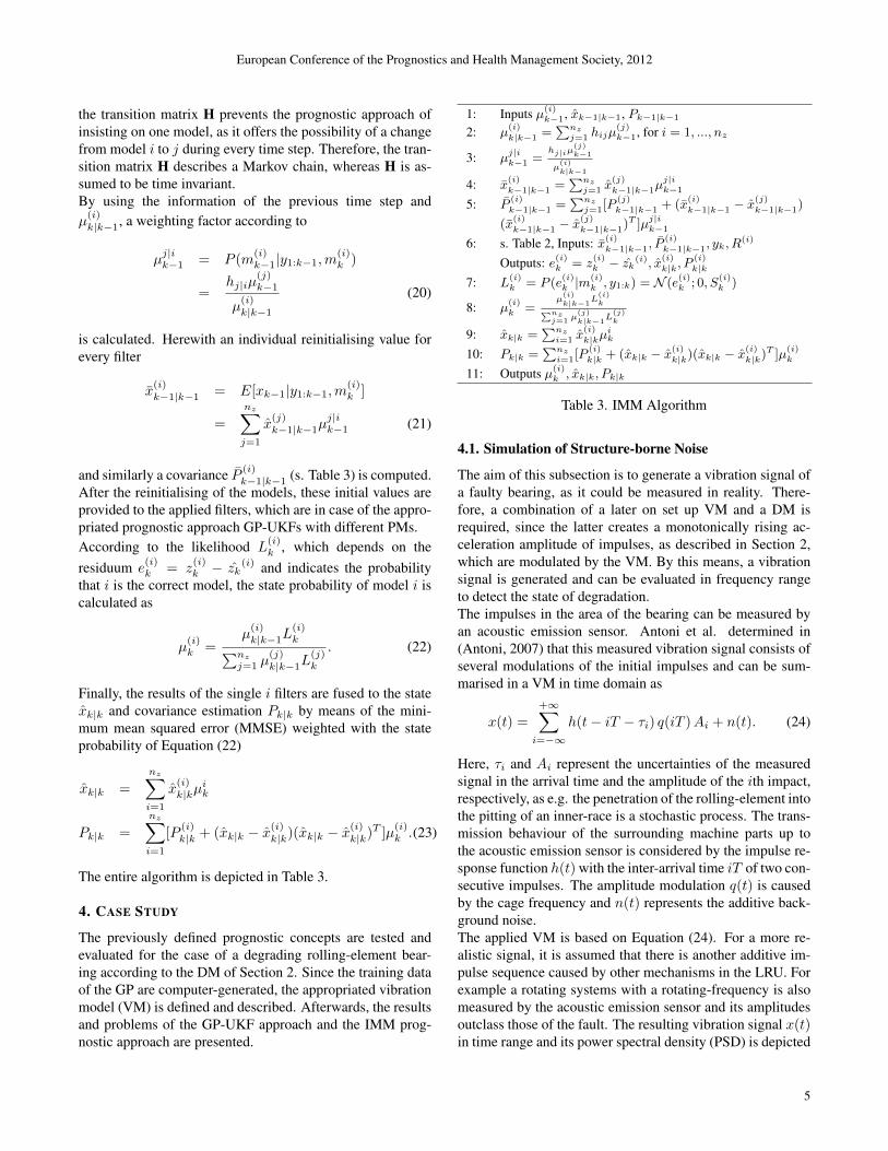
The entire algorithm is depicted in Table 3.

4. CASE STUDY

The previously defined prognostic concepts are tested andevaluated for the case of a degrading rolling-element bear-ing according to the DM of Section 2. Since the training dataof the GP are computer-generated, the appropriated vibrationmodel (VM) is defined and described. Afterwards, the resultsand problems of the GP-UKF approach and the IMM prog-nostic approach are presented.

1: Inputs µ(i)k−1, xk−1|k−1, Pk−1|k−1

2: µ(i)

k|k−1 =∑nzj=1 hijµ

(j)k−1, for i = 1, ..., nz

3: µj|ik−1 =

hj|iµ(j)k−1

µ(i)k|k−1

4: x(i)

k−1|k−1 =∑nzj=1 x

(j)

k−1|k−1µj|ik−1

5: P(i)

k−1|k−1 =∑nzj=1[P

(j)

k−1|k−1 + (x(i)

k−1|k−1 − x(j)

k−1|k−1)

(x(i)

k−1|k−1 − x(j)

k−1|k−1)T ]µj|ik−1

6: s. Table 2, Inputs: x(i)

k−1|k−1, P(i)

k−1|k−1, yk, R(i)

Outputs: e(i)k = z

(i)k − zk

(i), x(i)

k|k, P(i)

k|k

7: L(i)k = P (e

(i)k |m

(i)k , y1:k) = N (e

(i)k ; 0, S

(i)k )

8: µ(i)k =

µ(i)k|k−1

L(i)k∑nz

j=1 µ(j)k|k−1

L(j)k

9: xk|k =∑nzi=1 x

(i)

k|kµik

10: Pk|k =∑nzi=1[P

(i)

k|k + (xk|k − x(i)

k|k)(xk|k − x(i)

k|k)T ]µ(i)k

11: Outputs µ(i)k , xk|k, Pk|k

Table 3. IMM Algorithm

4.1. Simulation of Structure-borne Noise

The aim of this subsection is to generate a vibration signal ofa faulty bearing, as it could be measured in reality. There-fore, a combination of a later on set up VM and a DM isrequired, since the latter creates a monotonically rising ac-celeration amplitude of impulses, as described in Section 2,which are modulated by the VM. By this means, a vibrationsignal is generated and can be evaluated in frequency rangeto detect the state of degradation.The impulses in the area of the bearing can be measured byan acoustic emission sensor. Antoni et al. determined in(Antoni, 2007) that this measured vibration signal consists ofseveral modulations of the initial impulses and can be sum-marised in a VM in time domain as

x(t) =

+∞∑i=−∞

h(t− iT − τi) q(iT )Ai + n(t). (24)

Here, τi and Ai represent the uncertainties of the measuredsignal in the arrival time and the amplitude of the ith impact,respectively, as e.g. the penetration of the rolling-element intothe pitting of an inner-race is a stochastic process. The trans-mission behaviour of the surrounding machine parts up tothe acoustic emission sensor is considered by the impulse re-sponse function h(t) with the inter-arrival time iT of two con-secutive impulses. The amplitude modulation q(t) is causedby the cage frequency and n(t) represents the additive back-ground noise.The applied VM is based on Equation (24). For a more re-alistic signal, it is assumed that there is another additive im-pulse sequence caused by other mechanisms in the LRU. Forexample a rotating systems with a rotating-frequency is alsomeasured by the acoustic emission sensor and its amplitudesoutclass those of the fault. The resulting vibration signal x(t)in time range and its power spectral density (PSD) is depicted

5


0 4 · 10−2 8 · 10−2 0.14

−100

0

100

time t/s

x/10−

2m/s

2

(a)

102 102.5 103 103.50

5

10

frequency f/Hz

PSD

ofx

(b)

102 102.5 103 103.50

5

10

frequency f/Hz

PSD

ofxenv

(c)

Figure 2. (a) vibration signal x(t) in time range, (b) PSD ofx(t) with the marked fault frequency ff = 127Hz, (c) PSDof the envelope of x(t)

in Figures 2a and 2b, respectively. In Figure 2b, there is amark at the fault frequency ff = 127Hz, as a fault was as-sumed to be localised at the inner-race.The vibration signal in time range is dominated by the back-ground noise and the impact sequence of other mechanismswith a frequency of fo = 20Hz. In Figure 2b the as-sumed system behaviour of a second-order lag element withan eigenfrequency of fSB ≈ 1600Hz representing the pathbetween the bearing and the sensor is clearly visible in con-trast to the impulses caused by the fault, which are almostovershadowed by the background noise.By the application of an envelope xenv of the original vibra-tion signal, the influence of the system behaviour is reduced,as depicted in Figure 2c. Besides the impulse sequence and itsmodes, the amplitude of the fault frequency can be scanned.The amplitude of the PSD at the fault frequency is relatedto the amplitude given by the DM and therefore is an appro-priate feature for the prognostic process, as it determines thecurrent state of degradation. In addition the sidebands causedby the cage modulation q(t) at the frequency f = ff ± fcwith an expected cage frequency fc = 20Hz get visible.

0 50 100 150 2000

20

40

60

cycle

pitti

ngsu

rfac

eA

/µm

2

(a)

0 50 100 150 2000

10

20

cycle

feat

ure

(b)

Figure 3. simulated degradation of a rolling-element bearing(a) real degradation as the result of Equation (1), (b) measurednormed degradation of sampling the PSD generated by thepreviously set up VM at the fault frequency

The comparison of the real degradation of the applied DMin Equation (1) and the feature rfeat is depicted in Figure 3,whereas the applied loading is given in Figure 1b. The mea-sured degradation is quite noisy due to the background noisethat dominates the PSD of the vibration signal in lower fre-quency range. It indicates a different course compared tothe real degradation due to the frequency analysis, but as italso denotes the monotonically rising character, the measuredamplitude directly correlates with the pitting surface in Fig-ure 3a, i.e. the current degradation.The prognostic range is set within the normed feature bound-ary rfeat ∈ [0.001, 1], which is related to a pitting surfacerange of A ∈ [5µm2, 70µm2]. So this measured degradationcourse is applied for training and testing the GP-UKF prog-nostic concepts.

4.2. Applied Performance Metrics

To analyse the prognostic performance, several performancemetrics have to be applied. Those metrics can be one singleanalytical characteristic for the entire prediction or a graphi-cal depiction of every prediction step. Selected performancemetrics are summarised by Saxena et al. in (Saxena et al.,2008), whereas a few of these are used for evaluation of theappropriated prognostic concept in the following sections.Some notations of the metrics domain are given in the follow-ing glossary:

UUT Unit under testEOL End of life

6


EOP End of prediction - predicted failure featurecrossed threshold

i Time indexl Number of UUT indexP Time index of the first predictionL Total number of predictionsλ Normed time range of the entire predictionrl(i) Estimation of RUL at time step ti for the lth

UUTrl∗(i) Real RUL at time step ti

In the following subsections the applied performance metricsare defined.

4.2.1 Error

The error ∆l(i) indicates the difference between the predictedRUL and the true RUL in time step i

∆l(i) = rl∗(i)− rl(i) (25)

The error is one of the basic accuracy indicators and is, there-fore, included directly or indirectly in most of the selectedmetrics.

4.2.2 Average Bias

By averaging the error w.r.t. the entire prediction range, theaverage bias AB of lth UUT is defined as

ABl =

∑EOPi=P ∆l(i)

EOPl − Pl + 1(26)

Thus, the perfect score of ABl is zero.

4.2.3 Mean absolute percentage error

The Mean Absolute Percentage Error (MAPE) can be writtenas

MAPE(i) =1

L

L∑i=1

∣∣∣∣100∆l(i)

rl∗(i)

∣∣∣∣ . (27)

As it contains the error w.r.t. the actual RUL, derivations inearly states of prediction are not as weighted as those near theEOP.

4.2.4 Mean squared error

One most commonly used metric is the Mean Squared ErrorMSE, since it averages the squared error w.r.t. the numberof predictions L

MSE(i) =1

L

L∑i=1

∆l(i)2 (28)

An advantage in comparison to the average bias is that theMSE considers both negative and positive errors, as theaverage bias decreases at the appearance of positive andnegative derivations within one prediction.

4.2.5 Prognostic horizon

The Prognostic horizon PH describes the difference betweenthe EOP and the current time step i

PH(i) = EOP − i, (29)

whereas the PH can be dictated to fulfill certain specifica-tions. Those are e.g. to remain within a given constant errorbound depending on an accuracy value α, i.e.

[1− α] · rl∗ ≤ rl(t) ≤ [1 + α] · rl∗, (30)

comparable to the metrics in the following last subsection.Throughout the whole expectations the accuracy value is α =0.05.

4.2.6 α - λ Performance

Similarly to the PH, the α - λ Performance describes the timespan, when the predicted RUL remains within a given errorbound. In comparison to the PH, the bound decreases linearlyaccording to

[1− α] · rl∗(t) ≤ rl(t) ≤ [1 + α] · rl∗(t). (31)

Like the MAPE of Equation (27), this metric favours earlypredictions at λ ≈ 0 and tightens the demands for predictionsnear EOP (λ ≈ 1). Throughout the whole expectations theaccuracy value α of the α - λ accuracy is α = 0.20.

4.3. Prognostic Results of GP-UKF Approach

The aim of this section is to evaluate the GP-UKF approach.In Figure 4, four different test trials are depicted, whereas allcourses were generated by the DM in Equation (1). How-ever, the difference especially between trial 1 and 4 in termsof RUL at the beginning of the observation is obvious. There-fore, trial 2 has a similar course to trial 3 with nearly the samelife cycle.In Figure 4b, the corresponding features scanned at the faultfrequency ff = 127Hz in the PSD are given, which show aslightly different character in comparison to the real degrada-tion. The noise increases at higher degradation and is filteredby a low-pass filter with regard to the GP training. In Figure 5,the results of the GP training using trial 3 is shown, whereasthe estimated training and the real degradation is overlaid bythe estimated test degradation.The results of both the state estimation and the prediction ofdata set 2 and 3 using the UKF are presented in Figure 6.To compare the state estimation performance, the real featurecourse is also plotted. The first prediction started at cycle 2,whereas the following predictions began every 10 cycles later.The state estimation of data set 2 matches the real course rec-ognizably. But also the predictions show a high accuracy withan initial error ∆(2)(i = 2) ≈ 2 cycles. In sum, all predic-tions represent the behaviour of the damage course of trial 2.When the GP-UKF is trained and tested with data set 3, theprediction performance becomes slightly worse, as the error

7


0 100 200 3000

20

40

60

cycle

pitti

ngsu

rfac

eA

/µm

2

trial 1 trial 2 trial 3 trial 4

(a)

0 100 200 3000

10

20

cycle

feat

ure

trial 1 trial 2 trial 3 trial 4

(b)

Figure 4. four applied data sets, (a) real degradation, (b) fea-ture

of the forecast RUL of early predictions is about 20 cycleslower than the real RUL. However, later predictions (≈ 6th)match the real degradation with an accuracy allowing the pre-diction of the RUL.The same aforementioned behaviour is depicted in severalperformance metrics, summarised in Table 4. The two simi-lar metrics PH and α-λ accuracy are given as fractions of thenormed prediction range λ to indicate the time range, whenthe predictions fulfill the specifications until the EOP. Addi-tionally, the RUL is also normed to allow comparison of thefour trials with different RUL.In general, the predictions of all four trials show a high ac-

0 5 10 15 200

0.1

0.2

0.3

degradation r

deriv

atio

n∆r

real r est r tr est r test

Figure 5. training of the GP with data set 3

0 50 100 150 200 2500

0.5

1

cycle

feat

ure

state estimation real feature predictions

(a)

0 50 100 150 2000

0.5

1

cycle

feat

ure


(b)

Figure 6. the state estimation and prediction of (a) data set 2and (b) data set 3 in comparison to the real degradation course

Performance AB MSE MAPE α - λ PHMetric

Data Set 1 −0.21 21.79 19.52 1 0.86Data Set 2 0 10.87 13.11 1 1Data Set 3 −3.48 78.71 24.55 1 0.81Data Set 4 −2.28 56.44 23.86 1 0.84

Table 4. performance metrics of the four trials tested withthemselves

curacy, since every trial remains within the given α-λ errorbound during the entire prediction range and also satisfies thetighter specification of the PH after 20% of the normed pre-diction range λ, as displayed in Figure 7. Therefore, everytrial converges to the actual RUL with only slight deviationsat 0.3 λ. Additionally, all predictions indicate a rather conser-vative character, since the AB of all trials is mainly negative.In sum, the selected metrics correspond with the graphicalresults of Figure 6. The appropriated GP-UKF prognosticconcept offers a high accuracy for long turn prediction of arolling-element bearing, in case of the degradation followingthe model the filter is trained with.

4.4. Generalisation of the Prognostic Approach

Now the prognostic results of a GP-UKF that is tested witha degradation course, which differs from the training set, arediscussed as it occurs in real applications. Figure 8a and 8b

8


0 0.2 0.4 0.6 0.8 10

0.5

1

λ

RU

L

accuracy span pred. RUL Tr/Test 1pred. RUL Tr/Test 2 pred. RUL Tr/Test 3pred. RUL Tr/Test 4 real RUL

(a)

0 0.2 0.4 0.6 0.8 10

0.5

1

λ

RU

L

accuracy span pred. RUL Tr/Test 1pred. RUL Tr/Test 2 pred. RUL Tr/Test 3pred. RUL Tr/Test 4 real RUL

(b)

Figure 7. (a) prognostic horizon of the four given trials atα = 5%, (b) α-λ accuracy at α = 20%

show the results of the state estimation and prediction of trial1 and 4, respectively, when the prognostic model is trainedwith the data of trial 2. Additionally, the real degradationis plotted. The state estimation of both sets is satisfactory,since there are only slight deviations over the whole prognos-tic range. The predictions generally indicate the course ofthe training data set 2 with a progressive degradation at thebeginning and a flat degradation rate at the end of the life cy-cle, whereas both characteristics differ from the tested sets.Therefore, the forecast degradations are not as convincing asin comparison to Section 4.3, according to expectations.


Data Tr 2 Test 1 44.64 3522.93 242.65 0 0.07Data Tr 2 Test 4 8.64 544.8 116.60 0 0.04Data Tr 3 Test 1 22.79 1514.79 151.34 0 0.071Data Tr 3 Test 4 −28.12 1172.28 149.59 0 0.28

Table 5. performance metrics of different test data sets, whenGP is trained with data set 2

The performance is analysed again by means of the metricsin Table 5. Additionally, the prognosis performance in caseof training data set 3 is depicted. Compared to the results of

0 50 100 150 2000

0.5

1

cycle

feat

ure


(a)

0 100 200 3000

0.5

1

cycle

feat

ure


(b)

Figure 8. the state estimation and prediction of (a) data set 1and (b) data set 4 with the GP trained with data set 2

the previous section, all metrics increased considerably dueto both aforementioned causes of different degradation be-haviour of test and training sets and slightly inaccurate stateestimation. Hereby the predictions from cycle 60 to 90 (cor-responds to λ ≈ 0.5) of test data set 1 and at the end of dataset 4 are not able to predict the real damage course. These de-viations are also depicted in the graphical metrics in Figure 9,whereas neither the specifications of α-λ accuracy nor of thePH are fulfilled satisfactory.In comparison to training data set 3, the predictions with a dy-namic GP trained with data set 2 show beneficial prognosticresults in case of test data set 4 according to Table 5, whereasw.r.t. test data set 1 the third data set is advantageous. There-fore, a combination of both training data sets through a mul-tiple model approach is assumed to exhibit benefits in com-parison to the GP-UKF with only one set of training data.

4.5. Improvements by means of Multiple Model Approach

The prediction performance of an IMM approach with twodifferent GP-UKFs is discussed in this section. The two mod-els are the GP-UKF trained with trial 2 and 3, respectively, asthe combination of both is supposed to indicate the benefitsof the IMM approach.In Figure 10, the state estimation and prediction results oftest set 1 and 4 are depicted. The real degradation of bothtest cases is estimated very accurately with only a slight devi-

9


0 0.2 0.4 0.6 0.8 10

0.5

1

1.5

λ

RU

L

accuracy span pred. RUL Tr/Test 2/1pred. RUL Tr/Test 2/4 pred. RUL Tr/Test 3/1pred. RUL Tr/Test 3/4 real RUL

(a)

0 0.2 0.4 0.6 0.8 10

0.5

1

1.5

λ

RU

L

accuracy span pred. RUL Tr/Test 2/1pred. RUL Tr/Test 2/4 pred. RUL Tr/Test 3/1pred. RUL Tr/Test 3/4 real RUL

(b)

Figure 9. (a) prognostic horizon of the two tested data sets 3and 4 with training data set 2 (α = 5%), (b) α-λ accuracy atα = 20%

ation in Figure 10a between cycles 50 and 60. At first sight,the prediction results show a similar performance comparableto the GP-UKFs of Section 4.4. Especially the first predic-tions determine the RUL rather inaccurately, since the error|∆(i = 2)| amounts in both cases about 60 cycles. As de-scribed in the previous section, both test sets differ from theapplied training sets, which causes poor reproduction of thedamage course. The mode probability of trial 1 in Figure 10bindicates the same reason, since especially at the beginningof the prediction neither of both training sets replicate the realdegradation to satisfaction and therefore the model probabil-ities µ(1)

k and µ(2)k are about 0.5. In comparison to Figure 8a,

the later predictions of the MM approach in Figure 10a indi-cate a more accurate RUL estimation due to the dominationof training set 3 that reproduces the test set 1 more precisely.In Table 6, the performance metrics of the IMM approach areshown. Due to the inaccurate forecasts at the beginning of theprognosis, the metrics values are comparable to Table 5.To identify the advantages of the IMM approach, the net dia-grams in Figure 12 give an overview of the collected results.They show the metrics normalised to the major value withina test trial. Since most metrics describe an inaccurate RUL

0 50 100 150 200 2500

0.5

1

1.5

cycle

feat

ure


(a)

0 20 40 60 80 100 120 140

0

0.5

1

cycle

mod

epr

obab

ility

Tr 2 Tr 3

(b)

Figure 10. prediction results of training sets 2 and 3 testedwith (a) trial 1 and (b) mode probability of training sets 2 and3 during prediction of trial 1


Data Tr 2,3 Test 1 25 1841.14 160.54 0 0.07Data Tr 2,3 Test 4 −7 895.32 132.99 0.04 0.12

Table 6. performance metrics of IMM with training set 2 and3 testing set 1 and 4

estimation with large values, the time range, when the pre-dictions fulfill the specifications of the α-λ and the PH errorbound, is exchanged for the time range those specificationsare not met, i.e. PHnet = 1− PH .The diagrams show the advantage of the IMM approach, as allmeasured performance metrics lie between the metrics of theGP-UKFs trained with one data set. That means this approachincreases the robustness of a bearing’s RUL prediction, as itprovides the possibility of discarding inaccurate models de-pending on the mode probability.However, since the MM approach consists of the two PMs,which both differ from the test sets, the prognostic perfor-mance is still hardly able to outperform the results of bothGP-UKFs with reference to Table 5 and Table 6. Especiallythe α - λ accuracy and PH of trial 1 (Figure 12a) of bothGP-UKFs indicate the same behaviour and, thus, an IMMapproach based on those models is not able to increase thisperformance.The great benefit of the increased robustness is assumed to

10


0 50 100 150 200 250 3000

0.5

1

1.5

cycle

feat

ure


Figure 11. prediction results of training trials 2 and 3 testedwith trial 4

raise by including more models with different degradationcourses. Especially a progressive degradation rate at the be-ginning of the prediction range in case of forecasting test set1 is expected to be beneficial concerning the prognosis per-formance.

(a)

(b)

Figure 12. comparison of the single performance metrics of(a) test data 1 and (b) test data 4

5. CONCLUSION

Two prognostic concepts based on the GP-UKF approach topredict the RUL of a rolling-element bearing were examinedin the context of a case study. The results showed that a dy-namic GP in combination with an UKF estimates the RUL

of a bearing very accurately, when the applied training data isequal to the trial data. If the training data differs from the trialdata, the GP-UKF is not able to forecast the degradation pre-cisely, but mainly insists on the characteristics of the traineddamage course. To solve this problem, an IMM approachbased on two different GP-UKF models has been evaluated. Itwas assumed that the IMM algorithm, restoring several prog-nostic models, is more likely to forecast a damage course ofan unknown trial. The results proved these expectations, sincethe robustness of the predictions was highly increased by theapproach.By incorporating more prognostic models into the IMM ap-proach, which should mainly differ from the applied GP-UKFs, this approach is expected to even outperform the prog-nostic results of a single GP-UKF. This will be in the focusof further research.

NOMENCLATURE

Symbols

A Pitting surface∆Ai Increase of surface during cycle i∆ui Loading difference during cycle ikA, ku Coefficients of applied degradation modelλ′, k′ Shape/scaling parameter of Weibull

distributionµ′ Expected value of Exponential distributionD Data setxn Inputs of GPX Input matrixyn Outputs of GPy Output matrixε Noise termµ Mean of modelΣ Covariance of modelK Kernel matrixσn Noise termk(xi, xj) Kernel functionσf Signal variance of Kernel functionW Distance measure weighting matrixGPµ Mean of GPGPΣ Covariance of GPx∗ Test inputθ Hyperparameters of GPrk Degradation at kth time step∆rk Degradation rate at kth time stepX ′ Degradation rate matrixDr Training data setG Transition functionQk Process noiseH Observation functionzk Observation at kth time stepRk Measure noise

11


δk Noise Termχ[i] Sigma pointsα′, κ Scaling parameters of UKFµ, Σ A priori mean/covariancewm, wc Weights of mean/covarianceZ [i]k Observation

Kk Kalman gainM Prognostic model setmi Prognostic model iµ

(i)k|k−1 Mode probabilityhij Entries of transition matrix Hx

(i)k−1|k−1 Reinitialising state of IMM

P(i)k−1|k−1 Reinitialising covariance of IMM

L(i)k Likelihood of model i

e(i)k Residuumµ

(i)k State probability of model ix(t) Total vibration signalh(t) Impulse responseτi, Ai Uncertainties of arriving impulse responseq(t) Amplitude modulationn(t) Background noiseff Fault frequencyfo Frequency of other mechanismsfSB Eigenfrequency of system behaviourxenv Envelope of x(t)fc Cage frequencyrfeat Degradation of feature∆l(i) Error of RUL predictionABl Average Bias of lth UUTMAPE(i) Mean absolute percentage errorMSE(i) Mean squared errorPH(i) Prognostic horizonα Accuracy value

Shortcuts

RUL Remaining Useful LifetimeLRU Line-replaceable UnitDM Degradation ModelPM Prognostic ModelGP Gaussian ProcessUKF Unscented Kalman FilterIMM Interacting Multiple ModelVM Vibration ModelPSD Power Spectral DensityTr Training

(See also Glossary in Section 4.2)

REFERENCES

Antoni, J. (2007). Cyclic spectral analysis of rolling-elementbearing signals: Facts and fictions. Journal of Soundand vibration, 304(3-5), 497–529.

Choi, Y., & Liu, C. R. (2006a). Rolling contact fatigue lifeof finish hard machined surfaces - Part 1. Model devel-opment. Wear, 261(5-6), 485–491.

Choi, Y., & Liu, C. R. (2006b). Rolling contact fatigue lifeof finish hard machined surfaces - Part 2. Experimentalverification. Wear, 261(5-6), 492–499.

Daigle, M., & Goebel, K. (2010). Model-Based Prognosticsunder Limited Sensing.

Julier, S. (2002). The scaled unscented transformation. InAmerican Control Conference, 2002. Proceedings ofthe 2002 (Vol. 6, pp. 4555–4559).

Ko, J., & Fox, D. (2011). Learning GP-BayesFilters viaGaussian process latent variable models. AutonomousRobots, 30(1), 3–23.

Ko, J., Klein, D., Fox, D., & Haehnel, D. (2007). GP-UKF: Unscented Kalman filters with Gaussian pro-cess prediction and observation models. In IntelligentRobots and Systems, 2007. IROS 2007. IEEE/RSJ In-ternational Conference on (pp. 1901–1907).

Li, X., & Jilkov, V. (2003). A survey of maneuvering targettracking—Part V: Multiple-model methods. In Proc.SPIE Conf. on Signal and Data Processing of SmallTargets (pp. 559–581).

Orchard, M. E., & Vachtsevanos, G. J. (2009). A particle-filtering approach for on-line fault diagnosis and failureprognosis. Transactions of the Institute of Measure-ment and Control, 31(3-4), 221–246.

Orsagh, R., Sheldon, J., & Klenke, C. (2003). Prognos-tics/diagnostics for gas turbine engine bearings. In Pro-ceedings of IEEE Aerospace Conference.

Rasmussen, C. E., & Williams, C. K. I. (2006). GaussianProcesses for Machine Learning.

Saxena, A., Celaya, J., Balaban, E., Goebel, K., Saha, B.,Saha, S., et al. (2008). Metrics for evaluating perfor-mance of prognostic techniques. In Prognostics andHealth Management, 2008. PHM 2008. InternationalConference on (pp. 1–17).

Schaab, J. (2011). Trusted health assessment of dynamicsystems based on hybrid joint estimation (Als Ms. gedr.ed.). Dusseldorf: VDI-Verl.

Sturm, A. (1986). Walzlagerdiagnose an Maschinen undAnlagen. Koln: TUV Rheinland.

Yu, W. K., & Harris, T. A. (2001). A New Stress-Based Fa-tigue Life Model for Ball Bearings. Tribology Trans-actions, 44(1), 11–18.

12

unscented kalman filter with gaussian process … kalman filter with gaussian process degradation...

Documents