unsteady aerodynamics of deformable thin airfoils€¦ · unsteady aerodynamics of deformable thin...

Unsteady Aerodynamics of Deformable Thin Airfoils

William Paul Walker

Thesis submitted to the Faculty of the

Virginia Polytechnic Institute and State University

in partial fulfillment of the requirements for the degree of

Master of Science

in

Aerospace Engineering

Mayuresh J. Patil, Chair

William J. Devenport

Robert A. Canfield

August 5, 2009

Blacksburg, Virginia

Keywords: Unsteady Aerodynamics, Deformable Airfoils

Copyright 2009, William Paul Walker

Unsteady Aerodynamics of Deformable Thin Airfoils

William Paul Walker

(ABSTRACT)

Unsteady aerodynamic theories are essential in the analysis of bird and insect flight.

The study of these types of locomotion is vital in the development of flapping wing aircraft.

This paper uses potential flow aerodynamics to extend the unsteady aerodynamic theory of

Theodorsen and Garrick (which is restricted to rigid airfoil motion) to deformable thin airfoils.

Frequency-domain lift, pitching moment and thrust expressions are derived for an airfoil

undergoing harmonic oscillations and deformation in the form of Chebychev polynomials.

The results are validated against the time-domain unsteady aerodynamic theory of Peters.

A case study is presented which analyzes several combinations of airfoil motion at different

phases and identifies various possibilities for thrust generation using a deformable airfoil.

Contents

1 Introduction 1

2 Background and Objectives 2

2.1 Literature Survey . . . . . . . . . . . . . . . . . . . . . . . . . . . . . . . . . 2

2.2 Objectives . . . . . . . . . . . . . . . . . . . . . . . . . . . . . . . . . . . . . 7

3 Aerodynamic Theory 9

3.1 Lift and Pitching Moment Derivation . . . . . . . . . . . . . . . . . . . . . . 9

3.1.1 Mathematical Preliminaries . . . . . . . . . . . . . . . . . . . . . . . 10

3.1.2 Noncirculatory Flow . . . . . . . . . . . . . . . . . . . . . . . . . . . 13

3.1.3 Noncirculatory Pressure and Forces . . . . . . . . . . . . . . . . . . . 16

3.1.4 Circulatory Flow . . . . . . . . . . . . . . . . . . . . . . . . . . . . . 19

3.1.5 Theodorsen’s Function . . . . . . . . . . . . . . . . . . . . . . . . . . 24

3.1.6 Total Lift and Pitching Moment Expressions . . . . . . . . . . . . . . 26

3.2 Thrust Derivation . . . . . . . . . . . . . . . . . . . . . . . . . . . . . . . . . 29

3.2.1 Thrust due to Pressure . . . . . . . . . . . . . . . . . . . . . . . . . . 29

3.2.2 Thrust due to Leading Edge Suction . . . . . . . . . . . . . . . . . . 30

3.2.3 Total Thrust Force . . . . . . . . . . . . . . . . . . . . . . . . . . . . 32

4 Verification of Aerodynamic Theory 35

4.1 Peters’ Unsteady Airloads Theory . . . . . . . . . . . . . . . . . . . . . . . . 35

4.2 Application of Peters’ Theory to Current Problem . . . . . . . . . . . . . . . 38

iii

5 Case Study 40

5.1 Lift and Pitching Moment Results . . . . . . . . . . . . . . . . . . . . . . . . 40

5.1.1 Reduction to Steady Thin Airfoil Theory . . . . . . . . . . . . . . . . 42

5.2 Thrust Results . . . . . . . . . . . . . . . . . . . . . . . . . . . . . . . . . . 44

6 Conclusions and Future Work 55

6.1 Conclusions . . . . . . . . . . . . . . . . . . . . . . . . . . . . . . . . . . . . 55

6.2 Future Work . . . . . . . . . . . . . . . . . . . . . . . . . . . . . . . . . . . . 56

Bibliography 58

Appendix A 61

iv

List of Figures

3.1 Chebychev Polynomials . . . . . . . . . . . . . . . . . . . . . . . . . . . . . . 11

3.2 Joukowski mapping . . . . . . . . . . . . . . . . . . . . . . . . . . . . . . . . 14

3.3 Velocity due to generalized airfoil shape . . . . . . . . . . . . . . . . . . . . . 15

3.4 Vortex locations . . . . . . . . . . . . . . . . . . . . . . . . . . . . . . . . . . 20

3.5 Theodorsen’s function . . . . . . . . . . . . . . . . . . . . . . . . . . . . . . 27

3.6 Fluid flow around leading edge . . . . . . . . . . . . . . . . . . . . . . . . . . 31

5.1 Phase of lift relative to airfoil motion . . . . . . . . . . . . . . . . . . . . . . 42

5.2 Phase of pitching moment relative to airfoil motion . . . . . . . . . . . . . . 43

5.3 Thrust coefficient due to the first 5 airfoil shapes . . . . . . . . . . . . . . . 46

5.4 Thrust coefficient due to h and α . . . . . . . . . . . . . . . . . . . . . . . . 47

5.5 Thrust coefficient due to h and κ . . . . . . . . . . . . . . . . . . . . . . . . 47

5.6 Thrust coefficient due to h and κ2 . . . . . . . . . . . . . . . . . . . . . . . . 48

5.7 Thrust coefficient due to h and κ3 . . . . . . . . . . . . . . . . . . . . . . . . 48

5.8 Thrust coefficient due to α and κ . . . . . . . . . . . . . . . . . . . . . . . . 49

5.9 Thrust coefficient due to α and κ2 . . . . . . . . . . . . . . . . . . . . . . . . 50

5.10 Thrust coefficient due to α and κ3 . . . . . . . . . . . . . . . . . . . . . . . . 51

5.11 Thrust coefficient due to κ and κ2 . . . . . . . . . . . . . . . . . . . . . . . . 51

5.12 Thrust coefficient due to κ and κ3 . . . . . . . . . . . . . . . . . . . . . . . . 52

5.13 Thrust coefficient due to κ2 and κ3 . . . . . . . . . . . . . . . . . . . . . . . 52

5.14 Thrust coefficient due to h, κ2 and κ3 (φκ2 = −π/2) . . . . . . . . . . . . . . 53

5.15 Thrust coefficient due to h, κ2 and κ3 (φκ2 = 0) . . . . . . . . . . . . . . . . 53

v

5.16 Thrust coefficient due to h, κ2 and κ3 (φκ2 = π/2) . . . . . . . . . . . . . . . 54

5.17 Thrust coefficient due to h, κ2 and κ3 (φκ2 = π) . . . . . . . . . . . . . . . . 54

A.1 Functions F and G as a function of 1/k . . . . . . . . . . . . . . . . . . . . . 63

vi

List of Tables

3.1 Velocity potential functions . . . . . . . . . . . . . . . . . . . . . . . . . . . 16

3.2 Lift force components . . . . . . . . . . . . . . . . . . . . . . . . . . . . . . . 28

3.3 Pitching moment components . . . . . . . . . . . . . . . . . . . . . . . . . . 28

3.4 Leading edge suction velocities . . . . . . . . . . . . . . . . . . . . . . . . . . 31

3.5 Thrust force due to h and α . . . . . . . . . . . . . . . . . . . . . . . . . . . 32

3.6 Thrust force due to κ . . . . . . . . . . . . . . . . . . . . . . . . . . . . . . . 32

3.7 Thrust force due to κ2 . . . . . . . . . . . . . . . . . . . . . . . . . . . . . . 33

3.8 Thrust force due to κ3 . . . . . . . . . . . . . . . . . . . . . . . . . . . . . . 33

4.1 Lift force components . . . . . . . . . . . . . . . . . . . . . . . . . . . . . . . 39

4.2 Pitching moment components . . . . . . . . . . . . . . . . . . . . . . . . . . 39

5.1 Lift and pitching moment amplitude and phase terms . . . . . . . . . . . . . 41

vii

Nomenclature

An airfoil shape coefficient

a joukowski mapping circle radius

b semichord

C(k) Theodorsen’s function

F (k) real component of Theodorsen’s Function

G(k) imaginary component of Theodorsen’s function

Hn(k) Hankel function

h plunge variable

h plunge amplitude

i imaginary number

Jn(k) Bessel function of the first kind

k reduced frequency

L total lift

LC circulatory lift

LNC noncirculatory lift

M total Pitching moment

MC circulatory Pitching moment

MNC noncirculatory Pitching moment

p pressure

p0 total pressure

p∞ free stream pressure

viii

Q circulatory airfoil motion expression

S leading edge suction

t time

T total thrust

Tn Chebychev polynomials

TL thrust due to pressure

TLES thrust due to leading edge suction

u velocity in x direction

u′ disturbance velocity in x direction

v velocity in y direction

v′ disturbance velocity in y direction

X x location in unmapped plane

Y y location in unmapped plane

Yn(k) Bessel function of the second kind

x x location in mapped plane

y y location in mapped plane

Γ point vortex circulation

α pitch variable

α pitch amplitude

γw wake vorticity per unit length

ε source/sink strength

κ curvature variable

κ curvature amplitude

κn higher Order shape terms

φ velocity potential

ϕ phase angle

ρ density

ω frequency

ix

Chapter 1

Introduction

Micro Air Vehicles (MAVs) are a growing area of research. Flapping wing MAVs are similar to

birds and insects, and are highly maneuverable. The aerodynamics of flapping wing aircraft

is highly unsteady. Furthermore, during flight, bird and insect wings undergo significant

aeroelastic deformations in addition to the prescribed rigid-body kinematics. Understanding

the physics behind pitching, plunging and deforming airfoils will help in the design of flapping

wing MAVs.

Analytical, frequency-domain, unsteady aerodynamics theory, such as Theodorsen [1]

and Garrick [2] theory, has proven quite useful in understanding aeroelastic stability and

thrust generation. However, Theodorsen and Garrick only modeled thin airfoils undergoing

rigid body motion. Extending this unsteady aerodynamics theory to deformable airfoils will

help in further understanding the unsteady aerodynamics and aeroelastic response of bird

and insect flight, and help in improving the design of MAVs.

Inviscid potential flow theory may not accurately model flows at low Reynolds num-

bers or flows which have significant viscous effects, but it will help in increasing funda-

mental understanding of the unsteady aerodynamic flow and aeroelasticity of flapping wing

MAVs. Furthermore, potential flow theory can serve as a check for verifying other more

complex/computational codes and methods used in design.

1

Chapter 2

Background and Objectives

2.1 Literature Survey

Much research has been done in unsteady wing and airfoil theory. Theodorsen used two

dimensional elementary flows, solutions to Laplace’s equation, to develop the velocity po-

tential functions for a pitching and plunging flat plate with a flap[1]. The flow around a

flat plate was modeled using Joukowski transformation which mapped the flow around a

circle to flow around a flat plate. The source/sink and vortex flows were used to satisfy

boundary conditions and Bernoulli’s equation was used to obtain the unsteady airloads on a

thin oscillating airfoil with a flap. Theodorsen assumed small perturbations, which implies

a flat wake behind the airfoil extending to infinity. The airfoil motion was restricted to be

harmonic. This assumption allowed the vortex sheet extending from the trailing edge to

infinity to be integrated leading to a solution in the form of Bessel functions. Through this

solution, Theodorsen showed that the lift due to circulation was a function of the reduced

frequency. Theodorsen’s function is useful in describing the effect of the wake on the airloads

as a function of reduced frequency.

Garrick extended Theodorsen theory to develop the thrust force generated by a flat

plate in unsteady flow[2]. Garrick approached the problem in two different ways. First, the

problem was solved using the principle of conservation of energy. The energy of the structural

2

Chapter 2. Background and Objectives

motion, which is the energy required to maintain the oscillations must be equal to the energy

of the wake plus the energy of the propulsive force. This energy method involved calculating

the average work done by the structural motion and the average energy in the wake over one

period of oscillation. These average energies are used to solve for the average energy done by

the propulsive force which is given as the average propulsive force multiplied by the velocity.

However, this method yields only the average propulsive force over a period of oscillation.

In actuality, the propulsive force is changing with time in a harmonic manner just like the

lift and pitching moment. Garrick also calculated the propulsive force directly by calculating

the leading edge suction and the component of the pressure in the horizontal direction.

The leading edge suction on an airfoil results from the flow reaching the stagnation

point, and turning to go around the leading edge. von Karman and Burgers showed the

leading edge suction velocity on a flat plate by developing a function for the vorticity at the

leading edge and finding the limit as leading edge radius approaches zero[3]. The leading

edge suction force can be derived from the Blasius formula, as shown in Katz and Plotkin[4].

The second thrust component is the force from the pressure on the airfoil in the

horizontal direction. Garrick showed that harmonic plunging will always lead to a positive

propulsive force. This is a useful tool in the development of MAV’s and the study of bird

and insect flight.

The problem of an airfoil that is initially at rest and started abruptly was solved by

Wagner[5]. For an airfoil at constant angle of attack, the lift starts at 50% of the steady

lift and asymtotically approaches the steady lift. This is due to the shed vortex initially

after the airfoil starts moving. As the airfoil moves away from the initial location, the bound

circulation gradually approaches a value.

The problem of an airfoil entering a sharp edged gust was investigated by Kussner[7].

Kussner developed a function to show how the lift changes as a function of time as an airfoil

is entering a gust, which was similar to Wagner’s function. The airfoil entering a gust is

slightly different than an abrupt start of motion. This is because the effective change in

angle of attack as the airfoil suddenly enters the gust acts over only part of the airfoil until

3


the entire airfoil is inside the region being effected by the gust, while the abrupt start of an

airfoil acts over the entire airfoil.

The relationship between Wagner’s and Theodorsen’s function was investigated by

Garrick[6]. He also showed relationships between Theodorsen’s function and Kussner’s

function[7].

The unsteady aerodynamics of an airfoil in non-uniform motion was addressed by

von Karman and Sears[8]. This theory derived the formulae for lift and pitching moment

for general non-uniform motion, unlike theories by Theodorsen, Wagner, and Kussner which

addressed specific flow situations. The theory shows the lift and pitching moment each to be

a sum of three components, quasi-steady lift, apparent mass, and wake vorticity contribution.

The equations for lift and pitching moment were applied to specific flow situations and shown

to match theories by Theodorsen, Wagner, and Kussner. Sears later applied Heaviside’s

operators to obtain more convenient results of this general theory[9].

The work of Theodorsen and Garrick involves the unsteady aerodynamics of oscillat-

ing wings with a constant free-stream velocity. The problem of unsteady aerodynamics on

thin airfoils with a non constant free stream velocity has been investigated by a number of re-

searchers. Isaacs derived a solution for the lift on an airfoil in a non constant free-stream[10],

and investigated in particular the case of a rotary wing aircraft in forward flight[11]. The

rotary wing case applied only to an airfoil at constant angle of attack. This was done by

assuming the free-stream velocity to be a constant value plus a sinusoidal term. However,

Isaacs did not account for the wake moving downward due to the inflow of the rotor. This

wake shape would be a type of distorted helix shape.

The problem of the rotary wing was also investigated by Loewy[12]. Loewy solved

the problem of a rotary wing with no forward velocity, as in a helicopter in hover. Therefore,

for each spanwise location, the free stream velocity is constant in time. Loewy developed

a solution for this problem similar to Theodorsen theory. Along with the usual assumption

of small disturbances, Loewy assumed the chord, amplitude of oscillation in effective angle

of attack and relative airspeed vary slowly enough with span to say that the aerodynamics

4


at each blade radius are essentially the same on either side. Essentially this assumption

eliminated three dimensional effects. The solution by Loewy allows for all the unsteady

motion of Theodorsen theory. The difference between Theodorsen theory and Loewy’s theory

is the wake shape. The wake for a rotary wing in hover is a helix shape. Loewy modeled this

in two dimensions with a layered wake, where the distance between the layers depends on the

inflow velocity to the rotor, the number of blades in the rotor, and the period of oscillation

of the rotor. This wake model resulted in a function of frequency similar to Theodorsen

theory. Loewy showed that for the case of a rotary wing in hover, the aerodynamic forces

have the same form as that for non-rotating wings. Replacing Theodorsen’s function with

Loewy’s function changes the problem from that of a thin airfoil in harmonic motion to that

of a rotary wing, undergoing harmonic motion.

The non constant free-stream velocity problem was also addressed by Greenberg[13].

In his work, Greenberg developed an extension to Theodorsen theory to take into account the

non constant free-stream, unlike Isaacs however, Greenberg made an assumption that wake

was sinusoidal, such as the wake model used by Theodorsen. Therefore, the wake propagates

downstream with a constant velocity. This allowed Greenberg to obtain a solution to the

non constant free-stream problem for unsteady airfoil motions as well as just an airfoil at

constant angle of attack. Greenberg showed, via a numerical example, that the use of the

sinusoidal wake compared well to the model used by Isaacs.

There have been a number of investigations into relating the methods of Theodorsen,

Garrick, Loewy, Greenberg, and Isaacs to the aerodynamics of bird and insect wings. Zbi-

kowski[14] obtained a solution for unsteady flow in a form similar to von Karman and Sears

on a wing which is pitching, plunging, and can take into account non constant free-stream,

similar to Greenberg’s work. This solution was given in several different forms, including

time and frequency domains. However, the wake is integrated to a certain point, which is a

function of time, and not to infinity. This allows for a more general form of the solution to

the problem investigated by Wagner[5].

Other work in the application of unsteady flow of thin airfoils to bird and insect

5


flight was done by Azuma and Okamoto[15]. Insects such as dragonflies have corrugated

shaped wings, which pitch and plunge, while maintaining the airfoil shape. Their work was

an extension of Theodorsen theory to a combination of flat plate airfoils to give a corrugated

wing shape. The theory uses a set of flat plates attached end to end at various angles. This

allows for any number of airfoil shapes, and as the number of elements used increases, a

smooth airfoil, such as a curved plate, can be obtained.

Further study into the energy of the harmonic oscillating airfoil system, and it’s

relationship to aeroelastic systems, has been presented by Patil[16]. Using the methods

derived by Theodorsen and Garrick, Patil expanded the view of energy transfer in aeroelastic

analyses. The flow of energy was previously viewed as flowing between the structural motion

and the flow. However, the energy transfer to the flow has two destinations, the wake and

energy into propulsive force. This was also shown by Garrick in his energy approach to

deriving the propulsive force for a harmonic oscillating wing. Using the expressions for

energy, and conservation of energy, Patil showed that there are three possible energy transfer

modes, which depend on the direction of the energy flow. This led to the conclusion that,

for a flutter mode, the horizontal force must be a drag, and for a thrust producing mode,

the oscillations are damped, meaning the energy must come from the structure to maintain

oscillations. Also it is possible to have a damped mode, which also produces drag, in which

case all the energy transfers to the wake. This proves very helpful in the study of aeroelasticity

for thin airfoils in an unsteady flow.

Aerodynamics of deformable airfoils was investigated by Peters[17]. The theory de-

veloped by Peters is a general theory for the airloads on a deformable wing of arbitrary shape

with any form of free stream velocity. Peters’ theory is comprised of two parts, the airloads

theory and the wake model[18]. The airloads theory was developed for a arbitrary airfoil

shape in terms of the Chebychev polynomials. Combinations of these polynomial shapes can

lead to any possible shape desired because they are a complete set of functions. The wake

model can be any model desired depending on the type of flow considered. Peters shows by

using wake models from Theodorsen, Garrick, Wagner and others that these classical theories

6


for a rigid airfoil motion can be completely recovered with his theory.

The aerodynamics of deformable airfoils was also investigated by Johnston[19]. John-

ston applied the general unsteady airfoil theory of von Karman and Sears to a general deform-

ing camberline. Examples of different deformation shapes such as NACA 4-series camberlines

and curved leading and trailing edges (not hinged) were given.

There has been much more work in the field of unsteady flow on airfoils, including

work by Glegg and Devenport, which investigates the problem of unsteady loading on an

airfoil with thickness[20]. Their work uses conformal mapping to get any desired airfoil

shape, instead of just a flat plate such as Theodorsen. The forces were derived from the

Blasius theorem. Robert Jones investigated the unsteady aerodynamics of a wing with finite

span[21]. Jones’ work comprised of correcting the angle of attack for the downwash velocity

generated by three dimensional effects. Other work has been done investigating the problem

of unsteady compressible flows, including work by Hernandes and Soviero[22].

2.2 Objectives

The aim of the present research is to extend the unsteady aerodynamic theories of Theo-

dorsen[1] and Garrick[2] to deformable airfoils. Analytic expressions for lift, thrust and pitch-

ing moment of a thin airfoil undergoing harmonic motion (including harmonically changing

deformation) is developed in the frequency domain. To be able to represent a general de-

formable airfoil, the airfoil deformation can be represented in terms of an infinite series of

polynomials. For the present research, Chebychev polynomials are used in order to verify

with Peters’ theory[17]; the first two polynomials account for rigid body motion and the rest

account for the deformations.

The extended theory is verified by confirming that it converges to the solution for

the rigid body motion given by Theodorsen[1] and Garrick[2]and then compared to a time

domain solution developed by Peters[17] for deformable airfoils.

Results are presented for the aerodynamic load on an airfoil undergoing harmonic

7


motion/deformation corresponding to the first few deformation shapes. The lift and pitching

moment are calculated for harmonic oscillations corresponding to each individual polynomial

shape. The lift and pitching moment are linear and thus one can calculate the results for

oscillations made up of any combination of deformation shapes (with any relative magnitude

and phase) by superposition. The thrust is a nonlinear result and results are presented for

oscillation in just one shape as well as for various combinations of two deformation shapes

(with any relative magnitude and phase).

8

Chapter 3

Aerodynamic Theory

The deformable unsteady airloads theory presented in this research is based on earlier theories

developed by Theodorsen[1] and Garrick[2]. The theory is verified by the unsteady airloads

theory developed by Peters[18]. The derivation of the aerodynamic loads on a thin oscillating

deformable airfoil is presented in this chapter.

3.1 Lift and Pitching Moment Derivation

Theodorsen’s method for thin oscillating airfoils is based on ideal flow in two dimensions.

The elementary flows, which are solutions to Laplace’s equation, are combined to develop

the flow due to the disturbance of the airfoil in the flow, the flow due to circulation on the

airfoil, and the flow due to vortices in the wake. The sum of elementary flow solutions is

itself a solution to Laplace’s equation, because it is a linear differential equation. This allows

the superposition of flows, which allows for the separate development of the airloads due to

circulation and the airloads due to accelerations. Laplace’s equation is given as,

∇2φ = 0 (3.1)

where, φ is the velocity potential.

9

Chapter 3. Aerodynamic Theory

The airloads model is developed for a thin airfoil, essentially a flat plate. The method

in this derivation uses conformal mapping to develop the flow around the flat plate from the

flow around a circle in two dimensions. First, the noncirculatory flow is developed with a

source-sink pair sheet distributed along the chord. The strength of the sheet is derived from

the boundary condition of no flow through the surface of the airfoil. The circulatory flow is

derived by using a vortex sheet on the airfoil and in the wake, which extends to infinity. The

strength of this sheet is determined by the Kutta condition.

3.1.1 Mathematical Preliminaries

The Joukowski conformal mapping function, given below, is used to map the circle of radius,

b, centered at the origin to a flat plate of semichord, b. The mapping function maps all the

points outside of the circle to a location outside the the flat plate, points inside the circle to

a location outside the flat plate, but on a different Riemann surface, and the function maps

points on the circle directly to the flat plate[23].

x+ iy = X + iY +b2

X + iY(3.2)

The airfoil motion/deformation is represented by plunge, pitch, and different forms

of camber/deformation shapes. These shapes are defined by a set of complete orthogonal

polynomials so that one can represent any deformed shape by considering enough polynomials

in the solution. The orthogonal polynomials chosen for the present work are the Chebychev

polynomials. This was done to verify the results of this derivation with those of Peters. The

Chebychev polynomials are given as,

10


T0 (x) = 1

T1 (x) = x

Tn+1 (x) = 2xTn (x)− Tn−1 (x)

(3.3)

where, x is the non-dimensional variable along the chord varying from -1 at the leading

edge to 1 at the trailing edge. The first five polynomials, given below, and shown in Figure

3.1, are used in this derivation. However, this is a general derivation, and any number of

polynomials can be used to understand the unsteady aerodynamics of more complicated

deformation shapes.

T0 (x) = 1

T1 (x) = x

T2 (x) = 2x2 − 1

T3 (x) = 4x3 − 3x

T4 (x) = 8x4 − 8x2 + 1

(3.4)

−1 −0.5 0 0.5 1−1

−0.5

0

0.5

1

x

y

T0

T1

T2

T3

T4

Figure 3.1: Chebychev Polynomials

11


These polynomials are orthogonal on −1 ≤ x ≤ 1 with respect to a weight of

1/√

1− x2. There are other sets of functions which are directly orthogonal, such as the

Legendre polynomials. Chebychev are used because the results will be compared to Peters’

theory, which requires the use of Chebychev polynomials. The theory presented in this thesis

does not have this requirement and thus any complete set of orthogonal functions can be

used. The order of these polynomials determines the type of motion described by them. The

first Chebychev polynomial is a constant in space, which represents vertical displacement.

The time rate of change of vertical displacement is the plunge velocity. The second polyno-

mial is a linear function, which represents a flat plate at an angle to the flow, which is the

angle of attack. Likewise, the third polynomial is quadratic, which represents a quadratic

camber. This results in a generalized airfoil shape in terms of the Chebychev polynomials is

given as,

y(x) = A0T0(x) + A1T1(x) + A2T2(x) + ...+ AnTn(x) (3.5)

where, the An’s are the magnitude of each polynomial contributing to the complete airfoil

shape. This representation for a general airfoil shape is not very meaningful. The An’s can

be related to the classical airfoil shape variables, such as h for plunge and α for pitch. A0

is the plunge location, h/b. The second Chebychev polynomial is linear and corresponds to

the slope of the airfoil, and therefore A1 = α. The third Chebychev polynomial represents

curvature (or quadratic camber), but the second derivative of the polynomial is not one. To

give physical meaning to the shape, An’s are written in terms of the physically relevant defor-

mation variables by adding a scaling factor corresponding to the highest nonzero derivative.

Therefore it can be seen that the scaling factor multiplied by the Chebychev polynomials is

determined by the highest nonzero derivative. Therefore the airfoil deformation function is

given as,

12


y (x, t) =N∑n=0

AnTn

An =bn−1

∂nTn∂xn

∂nyn∂xn

y (x, t) =h

bT0 + αT1 +

bκ

4T2 +

b2κ2

24T3 +

b3κ3

192T4 + ...+ ANTN

(3.6)

3.1.2 Noncirculatory Flow

The noncirculatory part of the flow is solved using sources and sinks. The velocity potential

for the flow due to a source or a sink is given in as,

φsource/sink =ε

4πlog (X −X1)2 + (Y − Y1)2 (3.7)

where, ε is the strength of the source/sink, X and Y are non-dimensional spatial variables

in the unmapped domain, and X1 and Y1 are the location of the point source/sink.

Placing a double source of strength 2ε at a point (X1, Y1) and a double sink of strength

−2ε at (X1,−Y1), the source/sink pair velocity potential is found by summing the velocity

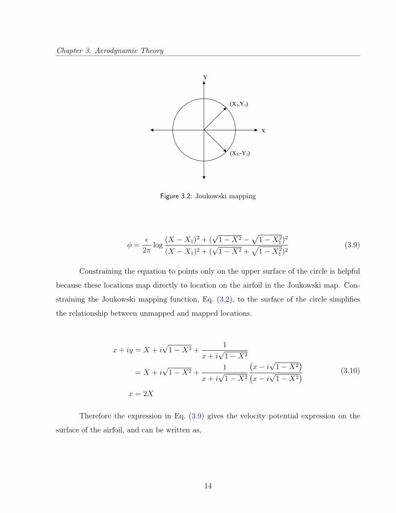
potential expressions. The conformal mapping representation of the wing in the unmapped

plane as a circle is shown in Figure 3.2. The velocity potential of the source/sink pair in the

unmapped plane is given as,

φsource/sink =ε

2πlog

(X −X1)2 + (Y − Y1)2

(X −X1)2 + (Y + Y1)2(3.8)

Y =√

1−X2 and Y1 =√

1−X21 for the upper surface of a circle. Thus, the velocity

potential can be written as,

13


(X1,-Y1)

(X1,Y1)

Y

X

Figure 3.2: Joukowski mapping

φ =ε

2πlog

(X −X1)2 + (√

1−X2 −√

1−X21 )2

(X −X1)2 + (√

1−X2 +√

1−X21 )2

(3.9)

Constraining the equation to points only on the upper surface of the circle is helpful

because these locations map directly to location on the airfoil in the Joukowski map. Con-

straining the Joukowski mapping function, Eq. (3.2), to the surface of the circle simplifies

the relationship between unmapped and mapped locations.

x+ iy = X + i√

1−X2 +1

x+ i√

1−X2

= X + i√

1−X2 +1

x+ i√

1−X2

(x− i

√1−X2

)(x− i

√1−X2

)x = 2X

(3.10)

Therefore the expression in Eq. (3.9) gives the velocity potential expression on the

surface of the airfoil, and can be written as,

14


φ =ε

2πlog

(x− x1)2 + (√

1− x2 −√

1− x21)2

(x− x1)2 + (√

1− x2 +√

1− x21)2

(3.11)

Integrating the expression for the source/sink pair along the chord gives a general

relationship for the velocity potential due to the source/sink pair sheet. This will be used to

describe all noncirculatory flows depending on the value of the strength, ε (x, t).

φ =b

2π

1∫−1

ε(x, t) log(x− x1)2 +

(√1− x2 −

√1− x2

1

)2

(x− x1)2 +(√

1− x2 +√

1− x21

)2dx1 (3.12)

The velocity generated by the source/sink pair must satisfy the no penetration bound-

ary condition. Thus, the velocity must be equal and opposite to the component of free stream

velocity minus the transverse velocity of motion of the airfoil at that point. Starting with

a general shape of the airfoil the disturbance flow needed to counteract the free stream flow

resembles Figure 3.3.

y(x,t)

y

x

u

u ∂y/∂x

є - ∂y/∂t

u

Figure 3.3: Velocity due to generalized airfoil shape

15


The strength of the source/sink sheet is determined by the boundary condition that

no flow penetrate the airfoil. Approaching the surface of the source/sink sheet, the velocity

must be perpendicular to the surface, and at this point the velocity of the fluid flowing out

of the source is the strength of the source[4]. Therefore, assuming small angles, the strength

of the source/sink sheet for a generalized airfoil shape, is given by,

ε(x, t) = u∂y

∂x+ b

∂y

∂t(3.13)

where, u is the free stream velocity.

The airfoil deformation expression, Eq. (3.6), can be substituted into the source/sink

strength equation given above, and this strength can be substituted into the velocity potential

equation, Eq. (3.12), leading to the potential for the noncirculatory flow as a function of x.

The velocity potential expressions for the first five airfoil shapes are shown in Table 3.1,

where the first two rows match Theodorsen[1]. These equations are functions of x only and

are valid for the upper surface of the airfoil. This is because the general equation for the

velocity potential, Eq. (3.12), was constrained to the upper surface of the circle. The pressure

on the airfoil due to these flows and the forces produced are derived in the following sections.

Table 3.1: Velocity potential functions

φh = 0 φh = hb√

1− x2

φα = uαb√

1− x2 φα = αb2

2x√

1− x2

φκ = ub2κ2x√

1− x2 φκ = − b3κ6

(1− x2)3/2

φκ2 = −ub3κ2

24(1− 4x2)

√1− x2 φκ2 = − b4κ2

24x (1− x2)

3/2

φκ3 = −ub4κ3

48x (1− 2x2)

√1− x2 φκ3 = b5κ3

720(1 + 6x2) (1− x2)

3/2

3.1.3 Noncirculatory Pressure and Forces

The desired result is ultimately the lift force and pitching moment, which requires the pres-

sure. Bernoulli’s equation gives the pressure using the velocity potential equations previously

16


developed. Bernoulli’s equation can be written as,

p0 = p+1

2ρV 2 + ρ

∂φ

∂t(3.14)

Solving this equation in the free-stream flow, the total pressure is given as,

p0 = p∞ +1

2ρu2 (3.15)

where, u is the free stream velocity. The Bernoulli equation is linearized for small disturbances

by assuming that the disturbance velocities in the x and y directions, u′ and v′, are small.

V = (u+ u′)i+ v′j → V 2 = (u2 + 2uu′) (3.16)

The linearized Bernoulli equation is given as,

p− p∞ = −ρ(u

b

∂φ

∂x+∂φ

∂t

)(3.17)

The difference in the velocity potential between two locations in space is the integral

of the velocity along the surface between these two locations,

φ2 − φ1 =

x2∫x1

u′dx (3.18)

where, x1 and x2 are locations in space and φ1 and φ2 are the velocity potential at those

locations respectively. Considering only the disturbance potential, the disturbance flow at

17


equal X locations on the circle, but opposite Y locations, must be the same. The integral of

the velocity from some X location on the upper side of the circle to the leading edge, and

the integral from the leading edge to the same X location on the lower half of the circle must

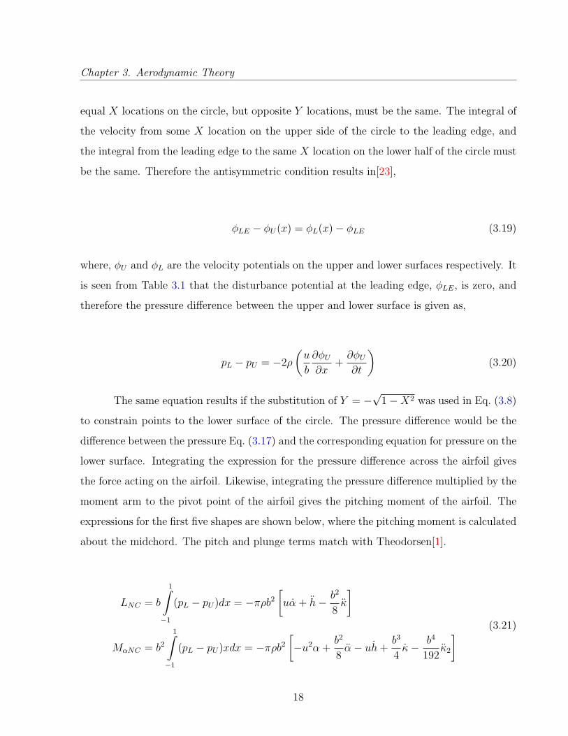
be the same. Therefore the antisymmetric condition results in[23],

φLE − φU(x) = φL(x)− φLE (3.19)

where, φU and φL are the velocity potentials on the upper and lower surfaces respectively. It

is seen from Table 3.1 that the disturbance potential at the leading edge, φLE, is zero, and

therefore the pressure difference between the upper and lower surface is given as,

pL − pU = −2ρ

(u

b

∂φU∂x

+∂φU∂t

)(3.20)

The same equation results if the substitution of Y = −√

1−X2 was used in Eq. (3.8)

to constrain points to the lower surface of the circle. The pressure difference would be the

difference between the pressure Eq. (3.17) and the corresponding equation for pressure on the

lower surface. Integrating the expression for the pressure difference across the airfoil gives

the force acting on the airfoil. Likewise, integrating the pressure difference multiplied by the

moment arm to the pivot point of the airfoil gives the pitching moment of the airfoil. The

expressions for the first five shapes are shown below, where the pitching moment is calculated

about the midchord. The pitch and plunge terms match with Theodorsen[1].

LNC = b

1∫−1

(pL − pU)dx = −πρb2

[uα + h− b2

8κ

]

MαNC = b2

1∫−1

(pL − pU)xdx = −πρb2

[−u2α +

b2

8α− uh+

b3

4κ− b4

192κ2

] (3.21)

18


The above equations give the airloads due to accelerations only. These equations are

derived assuming small disturbances relative to the free stream and the boundary condition

that no flow penetrate the surface of the airfoil.

3.1.4 Circulatory Flow

Thus far the model for the noncirculatory flow about a flat plate airfoil has been developed for

unsteady motions in the shape of Chebychev polynomials. The model satisfies the boundary

condition of no flow through the surface and yields a lift force and pitching moment. The

noncirculatory flow model however, does not satisfy the Kutta condition. This is seen by

evaluating the pressure difference equation for the noncirculatory flow at the trailing edge,

x = 1. This pressure difference should be zero to satisfy the Kutta condition. Therefore

there needs to be another flow included to account for this and assure that the flow will leave

the trailing edge in a smooth fashion.

The circulatory flow is developed by using a sheet of vortices on the body as well as

a sheet in the wake. The velocity potential for a point vortex is given as[4].

φvortex =Γ

2πtan−1 Y − Y1

X −X1

(3.22)

where, Γ is the strength of the vortex.

The wake vortex sheet moves downstream, along the x-axis, at the free stream velocity.

For a truly correct solution the wake vortex locations are a function of the airfoil motion; but

for small disturbances, a flat wake approximation will lead to negligible error. The magnitude

of the total shed wake circulation will be equal and opposite to the circulation on the airfoil,

and according the Kelvin’s circulation theorem, the combined magnitude of the airfoil and

wake circulation will be constant for all time[4].

The velocity potential for a pair of point vortices, one outside the circle in the wake

at X0 and the other of opposite strength at the image position inside the circle, 1/X0 is given

19


as,

φΓ0 =Γ

2π

[tan−1

(Y − Y0

X −X0

)− tan−1

(Y − Y0

X − 1X0

)](3.23)

where, Γ is the strength of each point vortex, and the variables X and Y are spatial variables

in the unmapped plane. The velocity perpendicular to the circle due to this vortex pair will

be zero when the vortices have the same strength. The equal and opposite strength vortices

secures the condition that the total circulation is zero in the domain and the no penetration

boundary condition is maintained. Note that these vortices will map to the same location in

the mapped plane, but on different Riemann surfaces. Figure 3.4 shows a conformal mapping

representation of the vortex pair.

1/X0 X0

Y

X

Figure 3.4: Vortex locations

Recalling the Joukowski mapping function, Eq. (3.2), points on the real axis map to

another location on the real axis. Therefore the vortex sheet in the mapped plane will be on

the real axis as in the unmapped plane. Using properties of tangents, Eq. (3.23) becomes,

20


φΓ0 =Γ

2πtan−1

(X − 1

X0

)Y

X2 −(X + 1

X0

)X + Y 2 + 1

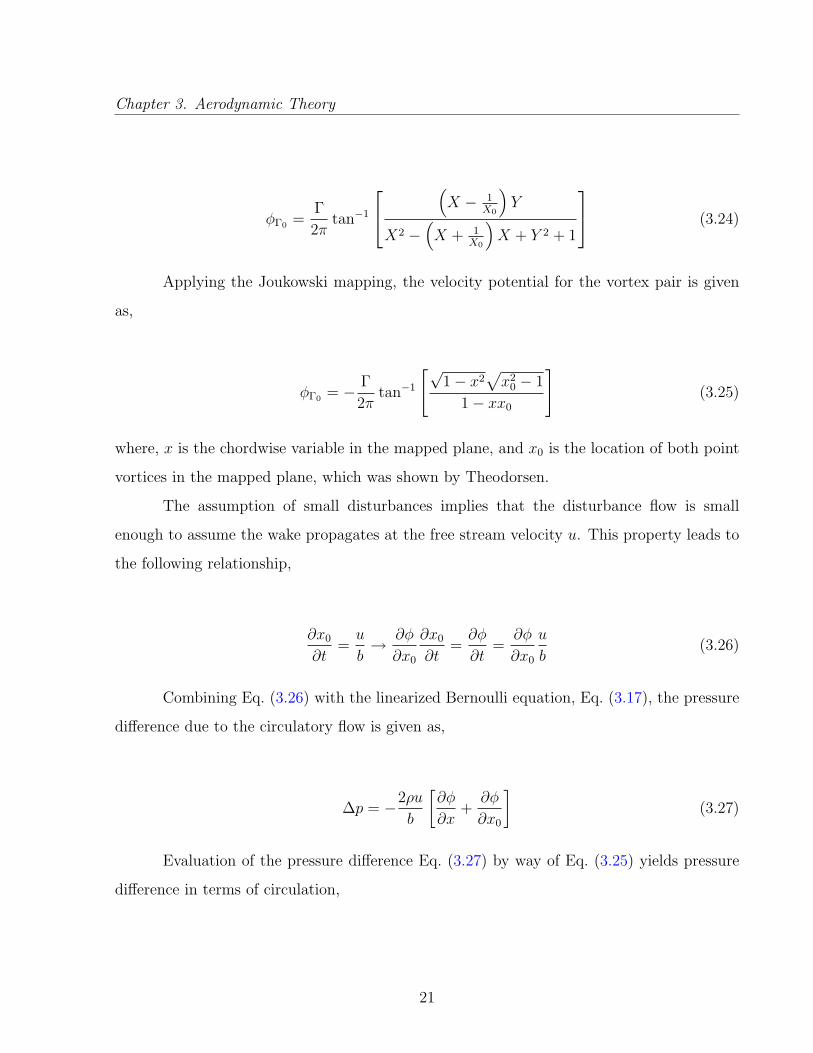
(3.24)

Applying the Joukowski mapping, the velocity potential for the vortex pair is given

as,

φΓ0 = − Γ

2πtan−1

[√1− x2

√x2

0 − 1

1− xx0

](3.25)

where, x is the chordwise variable in the mapped plane, and x0 is the location of both point

vortices in the mapped plane, which was shown by Theodorsen.

The assumption of small disturbances implies that the disturbance flow is small

enough to assume the wake propagates at the free stream velocity u. This property leads to

the following relationship,

∂x0

∂t=u

b→ ∂φ

∂x0

∂x0

∂t=∂φ

∂t=

∂φ

∂x0

u

b(3.26)

Combining Eq. (3.26) with the linearized Bernoulli equation, Eq. (3.17), the pressure

difference due to the circulatory flow is given as,

∆p = −2ρu

b

[∂φ

∂x+∂φ

∂x0

](3.27)

Evaluation of the pressure difference Eq. (3.27) by way of Eq. (3.25) yields pressure

difference in terms of circulation,

21


∆p = −ρubΓπ

[x0 + x

√1− x2

√x2

0 − 1

](3.28)

The lift on the airfoil due to the vortex pair comes from integrating the pressure

expression along the chord, and is given as,

LC = −ρuΓ

π

1∫−1

x0 + x√

1− x2√x2

0 − 1dx

LC = −ρuΓx0√x2

0 − 1

(3.29)

This is a continuous model; therefore the strength of the circulation shed into the

wake stretched along the x-axis is expressed as,

Γ = bγw (x0, t) dx0 (3.30)

where, γw (x0, t) is the circulation per unit length. Using this substitution, and integrating

the wake vortex sheet from the trailing edge to infinity, yields the circulatory lift,

LC = −ρub∞∫

1

x0√x2

0 − 1γw (x0, t) dx0 (3.31)

The velocity potential for the vortex sheet is given as,

φΓ = − b

2π

∞∫1

tan−1

[√1− x2

√x2

0 − 1

1− xx0

]γw (x0, t) dx0 (3.32)

22


The expression for the pitching moment is derived in the same fashion.

MC = −ρub2Γ

π

1∫−1

x0 + x√

1− x2√x2

0 − 1xdx

MC = −ρub2

2

∞∫1

{√x0 + 1

x0 − 1− x0√

x20 − 1

}γw (x0, t) dx0

(3.33)

The magnitude of the circulation, γw (x0, t), is determined by the Kutta condition.

The Kutta condition states that the flow must leave the trailing edge smoothly[4]. One way

to enforce this is to say that the pressure on the upper surface and lower surface at the

trailing edge are equal. Another way is to enforce that there be no infinite velocities at the

trailing edge, x = 1.

∂

∂x(φΓ + φα + φh + φα + φκ + φκ + ...+ φκN + φκN ) 6=∞ (3.34)

The terms in this equation are the disturbance velocities due to each deformation

shape and the circulation. The equations for the velocity potentials of each deformation

shape and the circulation are differentiated and evaluated at x = 1, the trailing edge. Stating

that the velocity be finite at the trailing edge results in a very useful equation for the first

five deformation shape.

1

2π

∞∫1

√x0 + 1

x0 − 1γw (x0, t) dx0 = uα + h+

b

2α +

ub

2κ

+ub2

8κ2 +

ub3

48κ3 = Q

(3.35)

This result is quite useful because the integral on the right hand side is shown to be

equal to a function of the airfoil motion, denoted as Q[1]. Eq. (3.35) is the exact same result

23


obtained by Theodorsen for the pitch and plunge terms. However, the deformation terms

are an extension to Theodorsen theory. Multiplying Eq. (3.31) by Q and dividing by the

integral on the right hand side of Eq. (3.35), the circulatory lift becomes,

LC = −2πρubQ

∫∞1

x0√x20−1

γw (x0, t) dx0∫∞1

√x0+1x0−1

γw (x0, t) dx0

(3.36)

which was shown by Theodorsen. The significance of the ratio of integrals is discussed in

detail further in the following section. The circulatory pitching moment is derived in the

same fashion as shown by Theodorsen[1].

MC = −πρub2Q

∫∞1 x0√x20−1

γw (x0, t) dx0∫∞1

√x0+1x0−1

γw (x0, t) dx0

− 1

(3.37)

The circulatory lift and pitching moment equations are the exact same as Theodorsen

derived. The only thing which makes this different is the airfoil motion term, Q, which

contains camber terms which Theodorsen did not have.

3.1.5 Theodorsen’s Function

Thus far there has been no mention of the time dependence of the motion other than it must

fit into a small disturbances assumption. Restricting the motion to be harmonic allows for

a solution to the ratio of integrals in Eqs. (3.36) and (3.37). The motion is written as a

function of frequency of oscillation by restricting the flow to simple harmonic motion in the

following form.

24


α (x, t) = αei(ωt+ϕα)

h (x, t) = hei(ωt+ϕh)

κ (x, t) = κei(ωt+ϕκ)

(3.38)

where, α, h and κ are magnitudes of oscillation. The terms ϕα, ϕh and ϕκ are the phase’s of

the motion. The frequency is denoted as ω.

The wake vortex sheet strength is also oscillatory, and is written in terms of the

reduced frequency, k = ωbu

.

γw (x, t) = γweiω(t− bxu ) = γwe

i(ωt−kx) (3.39)

where, γw is the magnitude of oscillation of the circulation.

The ratio of integrals in the circulatory loading expressions is denoted C, which was

shown by Theodorsen to be purely a function of the reduced frequency, k.

C =

∫∞1

x0√x20−1

γw (x0, t) dx0∫∞1

√x0+1x0−1

γw (x0, t) dx0

=γwe

iωtb∫∞

1x0√x20−1

e−ikx0dx0

γweiωtb∫∞

1

√x0+1x0−1

e−ikx0dx0

=

∫∞1

x0√x20−1

e−ikx0dx0∫∞1

√x0+1x0−1

e−ikx0dx0

= C (k)

(3.40)

This ratio of integrals over x0 is only a function of the reduced frequency, and take

the form of Hankel functions[23].

C (k) = F (k) + iG (k) =H

(2)1 (k)

H(2)1 (k) + iH

(2)0 (k)

(3.41)

25


where the Hankel functions in Eq. (3.41) are defined by a complex combination of Bessel

functions of the first and second kind in the form of,

H(2)n (k) = Jn (k)− iYn (k) (3.42)

Details of the solution to Theodorsen’s function are given in Appendix A.

A complex plot of Theodorsen’s function from reduced frequency values of zero to

infinity is shown in Figure 3.5. The function is 1 when the reduced frequency is zero and 0.5

when the reduced frequency is infinity. It reduces the amplitude of the circulatory lift with

increasing reduced frequency of oscillation. It also shifts the phase of the lift relative to the

motion.

Figure 3.5 gives much insight into the meaning of Theodorsen’s function. Essentially,

C(k) is a lift reduction factor as a function of the frequency of oscillation. Perhaps a very

important note is that this plot shows a value of reduced frequency where it could be sufficient

to assume a quasi-steady flow and ignore the effect of the wake and the higher order terms.

For values of 0 < k < 0.025, the flow could be assumed quasi-steady. Theodorsen’s function

being only a function of the reduced frequency in itself is a significant piece of information.

This shows that the reduced frequency is essentially the measure of the unsteadiness in the

flow, and therefore a flow with equal unsteadiness can be achieved with different combinations

of the frequency, chord length and free-stream velocity, as long as these combine to the same

value of reduced frequency.

3.1.6 Total Lift and Pitching Moment Expressions

The complete lift and pitching moment expressions are simply the addition of the circulatory

and noncirculatory components. The final lift expression is complex where the amplitude of

the complex number is the amplitude of oscillation, and the phase is the phase of the force

and moment relative to the phase of the motion. Using the harmonic motion of Eq. (3.38),

26


0 0.2 0.4 0.6 0.8 1−0.5

−0.4

−0.3

−0.2

−0.1

0

0.1

F(k)

G(k

)

Theodorsen’s Function

k=1

k=0.7

k=0.5k=0.3 k=0.18

k=0.1

k=0.05

k=0k=∞

C(k)

Figure 3.5: Theodorsen’s function

the different airfoil motions can have different phases relative to each other.

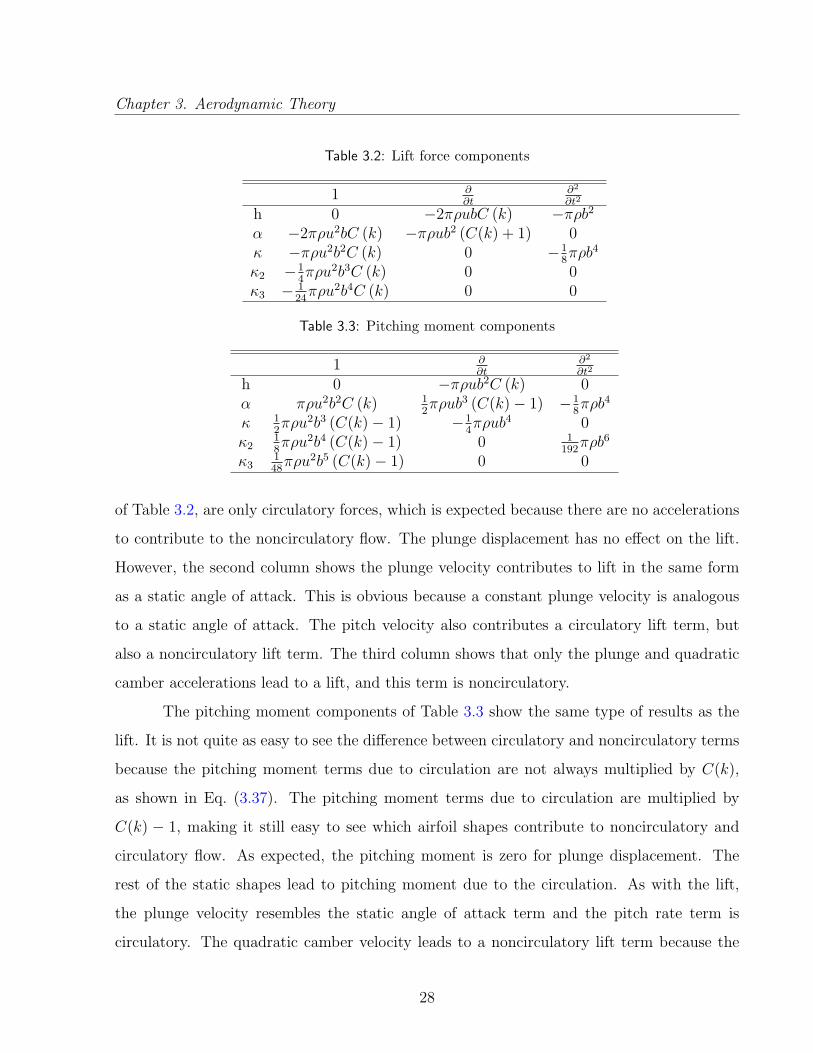
Tables 3.2 and 3.3 represent the lift and pitching moment contributions from each

shape. These tables give the airloads due to each deformation shape, corresponding velocities

and corresponding acceleration. The first two rows of each table match Theodorsen. The

top line represents the time derivative of the terms in the left column. The terms in the

table are multiplied by the respective derivative of the respective deformation variable. The

lift force components of Table 3.2 easily show which airfoil motion shapes contribute to the

lift. Moreover, the existence of Theodorsen’s function in the terms describes whether the lift

force is due to circulatory or noncirculatory flow. The static airfoil shapes, the first column

27


Table 3.2: Lift force components

1 ∂∂t

∂2

∂t2

h 0 −2πρubC (k) −πρb2

α −2πρu2bC (k) −πρub2 (C(k) + 1) 0κ −πρu2b2C (k) 0 −1

8πρb4

κ2 −14πρu2b3C (k) 0 0

κ3 − 124πρu2b4C (k) 0 0

Table 3.3: Pitching moment components

1 ∂∂t

∂2

∂t2

h 0 −πρub2C (k) 0α πρu2b2C (k) 1

2πρub3 (C(k)− 1) −1

8πρb4

κ 12πρu2b3 (C(k)− 1) −1

4πρub4 0

κ218πρu2b4 (C(k)− 1) 0 1

192πρb6

κ3148πρu2b5 (C(k)− 1) 0 0

of Table 3.2, are only circulatory forces, which is expected because there are no accelerations

to contribute to the noncirculatory flow. The plunge displacement has no effect on the lift.

However, the second column shows the plunge velocity contributes to lift in the same form

as a static angle of attack. This is obvious because a constant plunge velocity is analogous

to a static angle of attack. The pitch velocity also contributes a circulatory lift term, but

also a noncirculatory lift term. The third column shows that only the plunge and quadratic

camber accelerations lead to a lift, and this term is noncirculatory.

The pitching moment components of Table 3.3 show the same type of results as the

lift. It is not quite as easy to see the difference between circulatory and noncirculatory terms

because the pitching moment terms due to circulation are not always multiplied by C(k),

as shown in Eq. (3.37). The pitching moment terms due to circulation are multiplied by

C(k) − 1, making it still easy to see which airfoil shapes contribute to noncirculatory and

circulatory flow. As expected, the pitching moment is zero for plunge displacement. The

rest of the static shapes lead to pitching moment due to the circulation. As with the lift,

the plunge velocity resembles the static angle of attack term and the pitch rate term is

circulatory. The quadratic camber velocity leads to a noncirculatory lift term because the

28


changing shape results in local accelerations. Finally, the acceleration of the shapes leads to

noncirculatory terms.

There are almost no dynamic terms for the deformations. Most of the unsteady terms

come from the rigid body motion. The results of this derivation use Chebychev polynomials,

however, if a different set of orthogonal functions was used, these results would be different,

perhaps including more dynamic terms for the deformations.

3.2 Thrust Derivation

Force in ideal flow involves only nonviscous components, which for steady flow results in only

a lift force perpendicular to the direction of flow. Unsteady flows however can have force in

the horizontal direction parallel to the direction of flow. Depending on the airfoil motion,

this force can be either positive, which is a thrust, or negative, which is a drag. The following

derivation extends the method used by Garrick[2] to calculate the horizontal force for the

unsteady motion described by Eq. (3.6).

The force in the horizontal direction consists of two components, the component of

the pressure which acts in the direction of the flow, and the force due to leading edge suction.

The force due to leading edge suction will always be positive, as will be shown in this section,

and the component of the pressure in the flow direction can be either sign. The derivation

will be done assuming positive force in the negative x direction, which is the direction of

positive thrust.

3.2.1 Thrust due to Pressure

The component of the thrust due to the lift force is simply the net force multiplied by the

local slope. This expression is integrated along the chord to yield the thrust force due to a

general airfoil shape.

29


TL = b

1∫−1

∆p∂y

∂xdx (3.43)

3.2.2 Thrust due to Leading Edge Suction

The leading edge suction velocity comes from the vorticity at the leading edge. Referring

to Eq. (3.34), the velocity at the trailing edge x = 1 becomes finite. The leading edge

suction velocity is derived from the same equation, but at the leading edge, where x = −1.

Upon evaluating this equation at the leading edge, the velocity becomes infinite. This is

mathematically correct, but of course not physically possible. This airloads theory assumes

a thin airfoil, which is a flat plate. A true airfoil would have thickness associated with it,

and when the airfoil is at some angle of attack the stagnation point moves away from the

leading edge, x = −1 to some other location, as shown in Figure 3.6. The flow stops at the

stagnation point and must travel around the airfoil’s leading edge toward the other surface

and continue on. As the airfoil thickness decreases to zero, the leading edge radius also

approaches zero requiring the flow to turn exactly 180◦ at the exact point in the leading

edge, x = −1. This turn requires an infinite acceleration, and therefore an infinite velocity.

The true leading edge suction can be found by knowing the order of the infinity.

The leading edge suction goes to infinity in a functional form given by 1/√

1 + x as

shown by von Karman and Burgers[3]. Using this, the vorticity expression for the leading

edge is expressed as a function of the leading edge suction velocity.

2∂

∂x(φΓ + φα + φh + φα + ...+ φκN + φκN )x=−1 =

2S√1 + x

(3.44)

where S is the leading edge suction as shown by Garrick[2].

The derivative of the circulatory velocity potential term has an integral to infinity in

it which is the denominator of Theodorsen’s function. Using this and Theodorsen’s function,

30


V∞

V∞

Figure 3.6: Fluid flow around leading edge

along with Eq. (3.35), an expression for S is derived,

S =

√2

2(2C(k)Q−Q) +

[∂

∂x(φα + φh + φα + ...+ φκN + φκN )

√1 + x

b

]x=−1

(3.45)

The resulting leading edge suction velocity due to the first five airfoil displacement

/deformation modes are given in Table 3.4. The force due to this velocity is simply πρbS2[4].

The leading edge suction velocities for the pitch and plunge terms match Garrick[2].

Table 3.4: Leading edge suction velocities

1 ∂∂t

∂2

∂t2

h 0√

2C(k) 0

α√

2C(k)u√

22b (C(k)− 1) 0

κ√

22bu (C(k)− 1) 0 0

κ2

√2

8b2uC(k) 0 0

κ3

√2

48b3u (C(k)− 1) 0 0

31


3.2.3 Total Thrust Force

The thrust force due to both the lift component and the leading edge suction component

combine to result in Eq. (3.46). The squared term shows that drag will contain many

squared and cross coupling terms; and therefore the Tables following show each component

of the thrust up through the first five airfoil deformations. These tables are interpreted by

multiplying the terms in the table by the corresponding terms in the top row and left column.

T = TLES + TL = πρbS2 + b

1∫−1

∆p∂y

∂xdx (3.46)

Table 3.5: Thrust force due to h and α

h h α α

h 2πρbC(k)2 0 2πρub (2C(k)2 − C(k)) 2πρb2 (C(k)2 − C(k))

h - 0 −πρb2 0α - - 2πρu2b (C(k)2 − C(k)) πρub2 (2C(k)2 − 3C(k)− 1)α - - - 1

2πρb3 (C(k)2 − 2C(k)− 1)

The resulting expressions in Table 3.5 match the solution of Garrick [2]. There are no

thrust terms with plunge displacement in them, which is expected because a static flat plate

at no angle of attack will not produce any forces. The thrust force for pitching and plunging

motions is almost entirely dependent on circulatory terms. The plunge acceleration at an

Table 3.6: Thrust force due to κ

κ κ κ

h πρb2 (C(k)2 − C(k)) 0 0

h 0 0 0α 2πρu2b2 (C(k)2 − C(k)) 0 1

8πρb4

α 12πρb3 (2C(k)2 − C(k) + 1) 0 0

α −18πρb4 0 0

κ 12πρu2b3 (C(k)2 − C(k)) −1

4πρvb4 0

κ - 0 0κ - - 0

32


Table 3.7: Thrust force due to κ2

κ2 κ2 κ2

h 14πρub3 (2C(k)2 − C(k)) 0 0

h 0 0 0α 1

2πρu2b3 (C(k)2 − C(k)) 0 0

α 18πρub4 (2C(k)2 − 3C(k) + 1) 0 0

α 0 0 0κ 1

4πρu2b4 (C(k)2 − C(k)) 1

192πρb6 0

κ 0 0 0κ − 1

192πρb6 0 0

κ2132πρu2b5 (C(k)2 − C(k)) − 1

96πρub6 0

κ2 - 0 0κ2 - - 0

Table 3.8: Thrust force due to κ3

κ3 κ3 κ3

h 124πρub4 (2C(k)2 − C(k)) 0 0

h 0 0 0α 1

12πρu2b4 (C(k)2 − C(k)) 0 0

α 0 0 0α 1

48πρub5 (2C(k)2 − 3C(k)− 1) 0 0

κ 124πρu2b5 (C(k)2 − C(k)) 0 0

κ 0 0 0κ 0 0 0κ2

196πρu2b6 (C(k)2 − C(k)) 0 1

9216πρb8

κ2 0 0 0κ2 − 1

9216πρb8 0 0

κ31

1152πρu2b7 (C(k)2 − C(k)) − 1

4608πρub8 0

κ3 - 0 0κ3 - - 0

33


angle of attack results in a thrust term which is noncirculatory.

The camber terms of Tables 3.6 through 3.8 result in thrust terms, but mostly only

with the static shape multiplied by plunge and pitch terms. There are several terms including

camber rate and camber acceleration for the three different camber shapes listed, and they

are noncirculatory.

34

Chapter 4

Verification of Aerodynamic Theory

The theory developed in the previous chapter is an extension of unsteady aerodynamics

theories developed by Theodorsen and Garrick. This theory is based upon the solution

to Laplace’s equation for simple flows, the velocity potential approach, the no penetration

boundary condition on the airfoil surface, and the Kutta condition. This solution assumes

that the unsteady motion is harmonic. The lift, pitching moment, and thrust derived in

Chapter 3 match the solutions of Theodorsen and Garrick exactly for the rigid body motion

terms. However, the theory in Chapter 3 is not the only deformable airloads theory; a similar

theory has been developed by Peters. Peters’ theory is a general theory for any arbitrary

motion that requires the use of Chebychev polynomials to define the deformation shapes[17].

Peters has shown for the pitch and plunge cases, assuming the motion to be harmonic and

the wake to be flat, that Theodorsen theory can be recovered from his formulation. It follows

Peter’s theory will reduce to the extension to Theodorsen and Garrick theory derived in this

work.

4.1 Peters’ Unsteady Airloads Theory

The unsteady airloads theory developed by Peters is described briefly in this section in order

to show the equations which will be used in comparison to the theory in this work. Peters

35

Chapter 4. Verification of Aerodynamic Theory

expresses the no penetration boundary condition as,

w = v + λ

= u0∂h

∂x+∂h

∂t+ v0 + v1

x

b

(4.1)

where w is the total induced velocity, v is the velocity due to the bound vorticity, and

λ is the velocity due to the wake vorticity. The total induced velocity is a function of the

airfoil shape and motion, as shown in the second half of the equation. The airfoil shape is

given by h(x, t), and so the derivatives ∂h/∂x and ∂h/∂t are the local slope of the airfoil and

local vertical velocity of the airfoil as a function of the chordwise location x. The horizontal

and vertical free stream velocities are u0 and v0 respectively. The term v1 is the velocity

gradient and b is the semichord.

The velocity v is expressed as the distribution of vortices on the airfoil is given by

γb (ξ, t)[17].

v = − 1

2π

b∫−b

γb (ξ, t)

x− ξdξ (4.2)

The pressure difference across the airfoil is expressed for the body[17],

∆P = ρu0γb + ρ

x∫−b

∂γb∂t

dξ (−b < x < b) (4.3)

as well as for the wake[17],

0 = u0γw +∂Γ

∂t+ ρ

x∫b

∂γw∂t

dξ (b < x) (4.4)

36


Therefore applying the boundary condition of no penetration results in,

∂λ

∂t+ u0

∂λ

∂x=

1

2π

dΓdt

b− x(4.5)

where Γ is circulation[17].

These equations are solved using the Glauert change variable x = b cosϕ. The ex-

pressions for v, h and λ become,

v =∞∑n=0

γn cos(nϕ)

λ =∞∑n=0

λn cos(nϕ)

h(x) =∞∑n=0

hn cos(nϕ)

(4.6)

Using Eq. (4.6), the pressure difference is integrated along the chord yield the lift[17].

L = −2πρu0b (w0 − λ0)− πρu0bw1 − πρb2

(w0 −

1

2w2

)(4.7)

The pitching moment is found by integrating the pressure difference multiplied by the

moment arm x[17].

M = πρu0b (w0 − λ0)− 1

2πρu0bw2 −

1

8πρb2 (w1 − w3) (4.8)

Finally, the drag expression is given as[17],

37


D = −2πρb(h0 − λ0

)[(h0 − λ0

)+ u0

∞∑n=1

nhnb

]

+ 2πρ∞∑n=1

hn

[b

4

(hn−1 − hn+1

)+ nu0hn

]+ πρ

b

2h1h0

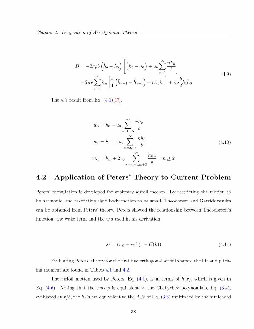
(4.9)

The w’s result from Eq. (4.1)[17],

w0 = h0 + u0

∞∑n=1,3,5

nhnb

w1 = h1 + 2u0

∞∑n=2,4,6

nhnb

wm = hm + 2u0

∞∑n=m+1,m+3

nhnb

m ≥ 2

(4.10)

4.2 Application of Peters’ Theory to Current Problem

Peters’ formulation is developed for arbitrary airfoil motion. By restricting the motion to

be harmonic, and restricting rigid body motion to be small, Theodorsen and Garrick results

can be obtained from Peters’ theory. Peters showed the relationship between Theodorsen’s

function, the wake term and the w’s used in his derivation.

λ0 = (w0 + w1) (1− C(k)) (4.11)

Evaluating Peters’ theory for the first five orthogonal airfoil shapes, the lift and pitch-

ing moment are found in Tables 4.1 and 4.2.

The airfoil motion used by Peters, Eq. (4.1), is in terms of h(x), which is given in

Eq. (4.6). Noting that the cosnϕ is equivalent to the Chebychev polynomials, Eq. (3.4),

evaluated at x/b, the hn’s are equivalent to the An’s of Eq. (3.6) multiplied by the semichord

38


Table 4.1: Lift force components

1 ∂∂t

∂2

∂t2

h0 0 −2πρu0bC (k) −πρb2

h1 −2πρu20C (k) −πρu0b (C(k) + 1) 0

h2 −4πρu20C (k) 0 −1

2πρb2

h3 −6πρu20C (k) 0 0

h4 −8πρu20C (k) 0 0

Table 4.2: Pitching moment components

1 ∂∂t

∂2

∂t2

h0 0 −πρu0b2C (k) 0

h1 πρu20bC (k) 1

2πρu0b

2 (C(k)− 1) −18πρb3

h2 2πρu20b (C(k)− 1) −πρu0b

2 0h3 3πρu2

0b (C(k)− 1) 0 18πρb3

h4 4πρu20b (C(k)− 1) 0 0

b. The free stream velocity u is u0 in Peters’ theory. Upon inspecting Tables 4.1 and 4.2, and

comparing to Tables 3.2 and 3.3, it is seen that both the formulations yield the same result.

The drag results have the same outcome except for the sign. This is because Peters’ sign

convention is for the positive force to be in the drag direction, while the extended Garrick

theory assumes the force positive in the thrust direction.

The solution for Peters’ theory relies on the use of the Glauert change variable, which

are the Chebychev polynomials at x/b. This is the reason these polynomials were chosen. The

results developed in this thesis are essentially Peters’ theory for an flat wake with harmonic

motion. However, the extended Theodorsen and Garrick theory derived can be formulated

for any set of orthogonal functions, such as the Legendre polynomials. This allows many

different shapes to be used instead of just Chebychev polynomials.

39

Chapter 5

Case Study

This chapter is focused on presenting various case studies based on the results of the airloads

derivation. Expressions for the amplitude of oscillation and phase of lift and pitching moment

relative to the motion is derived. A detailed study into the thrust and how the pressure and

leading edge suction components contribute to the thrust for each case, and combinations of

them is shown.

5.1 Lift and Pitching Moment Results

The lift and pitching moment, Tables 3.2 and 3.3, can easily be made a function of the reduced

frequency using the substitution of Eq. (3.38). Using this substitution, the expressions for

the lift and pitching moment will be expressed as,

L = Lei(ωt+ϕL) = LeiωteiϕL

M = Mei(ωt+ϕM ) = MeiωteiϕM(5.1)

where, L and M are the magnitudes of oscillation of the lift and pitching moment respectively;

and the ϕL and ϕM are the phase relative to the motion for lift and pitching moment

respectively. The time dependent term easily cancels from both sides of the equations.

40

Chapter 5. Case Study

Therefore the result yields an equation for the lift and pitching moment amplitudes and

phases relative to the airfoil motion. The coefficient expressions for the lift and pitching

moment amplitude and phase are given in Table 5.1. The lift and pitching moment terms

due to each shape can be found by multiplying the term by the left column.

Table 5.1: Lift and pitching moment amplitude and phase terms

LeiϕL MeiϕM

heiϕh πρu2 (k2 − i2kC(k)) iπρu2kC(k)

αeiϕα −πρu2b (2C(k) + ik + ikC(k)) πρu2b2(C(k)− ik + ik

2+ k2

8

)κeiϕκ −πρu2b2

(C(k) + k2

8

)12πρu2b3

(C(k)− 1− ik

2

)κ2e

iϕκ2 −14πρu2b3C(k) 1

8πρu2b4

(C(k)− 1− k2

24

)κ3e

iϕκ3 − 124πρu2b4C(k) 1

8πρu2b5 (C(k)− 1)

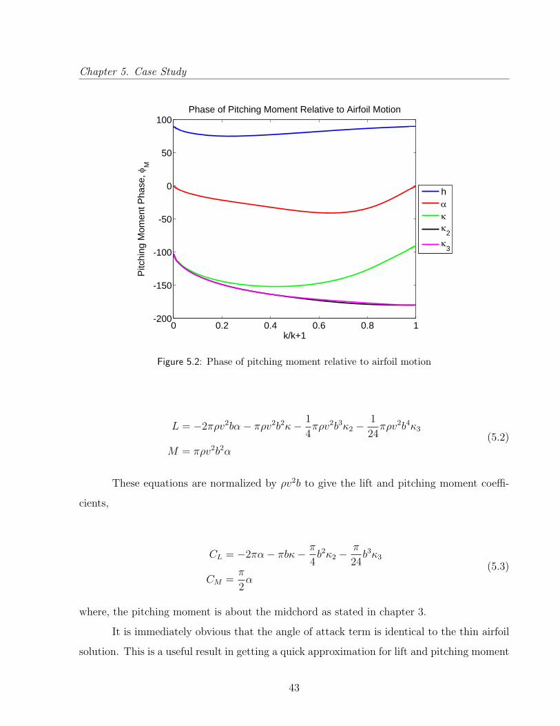
It can be seen that the magnitude of the lift and pitching moment terms will grow to

be very large as a function of reduced frequency. However, the phase angles of the lift and

pitching moment relative to the airfoil motion change due to the value of C(k). The phase

also changes due to the quasi-steady parts as reduced frequency grows large. Theodorsen’s

function changes the lift and pitching moment phase as reduced frequency increases. At the

point when reduced frequency reaches k ≈ 0.18, the phase shift reaches a maximum and as

reduced frequency continues to increase, the phase shift approaches it’s value when reduced

frequency is zero (see Figure 3.5). This phase shift effects only the circulatory lift. The phase

of the noncirculatory lift changes as reduced frequency grows large due to the quasi-steady

part of the lift and pitching moment. Figures 5.1 and 5.2 below show the phase of lift and

pitching moment, respectively, for each of the first five airfoil shapes alone as a function of

reduced frequency. In order to observe the entire range of reduced frequency, k/(k + 1) is

used instead of k. Therefore when this value is zero, k is zero, when it is 0.5, k is 1, and

when it is 1, k is infinity.

The plunge and pitch motion very easily show the effect Theodorsen’s function has

on the phase shift. The phase of the lift lags 90◦ with the plunge motion initially and at low

reduced frequencies the phase lags back even further as reduced frequency increases. For large

41


0 0.2 0.4 0.6 0.8 1-200

-150

-100

-50

0

50

100

150

200

k/k+1

Lift

Pha

se, φ

L

Phase of Lift Relative to Airfoil Motion

hακκ2κ3

Figure 5.1: Phase of lift relative to airfoil motion

k, the terms with the highest order in k in the lift expression become more prominent, while

other terms become more insignificant. For the plunge case, the imaginary part of the lift

expression becomes insignificant and the lift becomes in phase with the plunge motion. All

the airfoil motion types considered show similar trends, which is due to the non-circulatory

terms getting very large at high reduced frequency. This is because at high frequencies,

the motion is dominated more by accelerations than circulation. The κ2 term in Figure 5.1

directly coincides with the κ3 curve and cannot be seen.

5.1.1 Reduction to Steady Thin Airfoil Theory

This theory is developed on the basis of small disturbances. Classical steady thin airfoil

theory assumes the same. The lift and pitching moment results should easily reduce to

steady thin airfoil theory when the frequency is zero. Therefore the lift terms in Table 5.1

reduce to the following lift and pitching moment expressions when the reduced frequency is

zero. The value of C(k) is 1 when k = 0 and also ϕ will be zero for each case.

42


0 0.2 0.4 0.6 0.8 1-200

-150

-100

-50

0

50

100

k/k+1

Pitc

hing

Mom

ent P

hase

, φM

Phase of Pitching Moment Relative to Airfoil Motion

hακκ2κ3

Figure 5.2: Phase of pitching moment relative to airfoil motion

L = −2πρv2bα− πρv2b2κ− 1

4πρv2b3κ2 −

1

24πρv2b4κ3

M = πρv2b2α

(5.2)

These equations are normalized by ρv2b to give the lift and pitching moment coeffi-

cients,

CL = −2πα− πbκ− π

4b2κ2 −

π

24b3κ3

CM =π

2α

(5.3)

where, the pitching moment is about the midchord as stated in chapter 3.

It is immediately obvious that the angle of attack term is identical to the thin airfoil

solution. This is a useful result in getting a quick approximation for lift and pitching moment

43


for any polynomial camberline shape desired. Due to the use of the Chebychev polynomials,

the airfoil shape resulting in angle of attack results in a positive α being nose down. Therefore,

since lift is positive up, when a negative α is used, which would be nose up, the lift is positive.

The pitching moment is positive nose down. Therefore when a negative α is used, which is

nose up, the pitching moment is negative, as is should be from thin airfoil theory. The plunge

location, h, is positive up and κ is concave up.

5.2 Thrust Results

The thrust, like the lift and pitching moment is also an oscillatory term. However, the value

oscillates about an average value, and therefore the average thrust can be calculated for each

type of motion, and combinations of each type of motion. The thrust is a quadratic function

of the various motion types. This leads to cross coupling terms, as seen in Tables 3.5 through

3.8.

The average thrust can be obtained by integrating the thrust over one time period,

since the motion is harmonic. Harmonic motion takes the form sin(ωt+ϕ). When employing

the complex form of the airfoil motion, Eq. (3.38), the motion is specified as cos(ωt + ϕ) +

i sin(ωt+ ϕ). Only the sin or cos term is needed to specify the harmonic motion. Therefore

either the real or imaginary part of the lift and pitching moment equations can be used to

calculate the average thrust. Referring back to the equation for the thrust force, Eq. (3.46),

the imaginary part of each component is used to derive the average expressions below. Keep

in mind the real component would give the same result.

Taverage = πρbω

2π

2πω∫

0

Im[S]2dt+bω

2π

2πω∫

0

1∫−1

Im [∆p] Im

[∂y

∂x

]dxdt (5.4)

The final expression for the average thrust is lengthy and therefore not displayed.

However, the expressions for the individual airfoil motion types are much shorter due to the

44


absence of coupled terms. The thrust due to the first five airfoil motion types individually

are given as,

Th = h2k2πρu2

b

(F 2 +G2

)Tα = α2πρu

2b

4

((k2 + 4

)F 2 − 2

(k2 + 2

)F + k2 − 2Gk +G2

(k2 + 4

))Tκ = κ2πρu

2b3

4

(F 2 − F +G2

)Tκ2 = κ2

2

πρu2b5

64

(F 2 − F +G2

)Tκ2 = κ2

3

πρu2b7

2304

(F 2 − F +G2

)(5.5)

where, C(k) = F + iG.

The values of F and G are a complex combination of Bessel function which vary based

on frequency. The derivation of these is given in Appendix A. For the plunge only case, the

thrust is always positive[2]. The four airfoil shapes following may be positive or negative

based on the reduced frequency. The thrust due to κ, κ2 and κ3 are indirectly functions of

reduced frequency through F and G. Therefore, these thrust values will approach a value

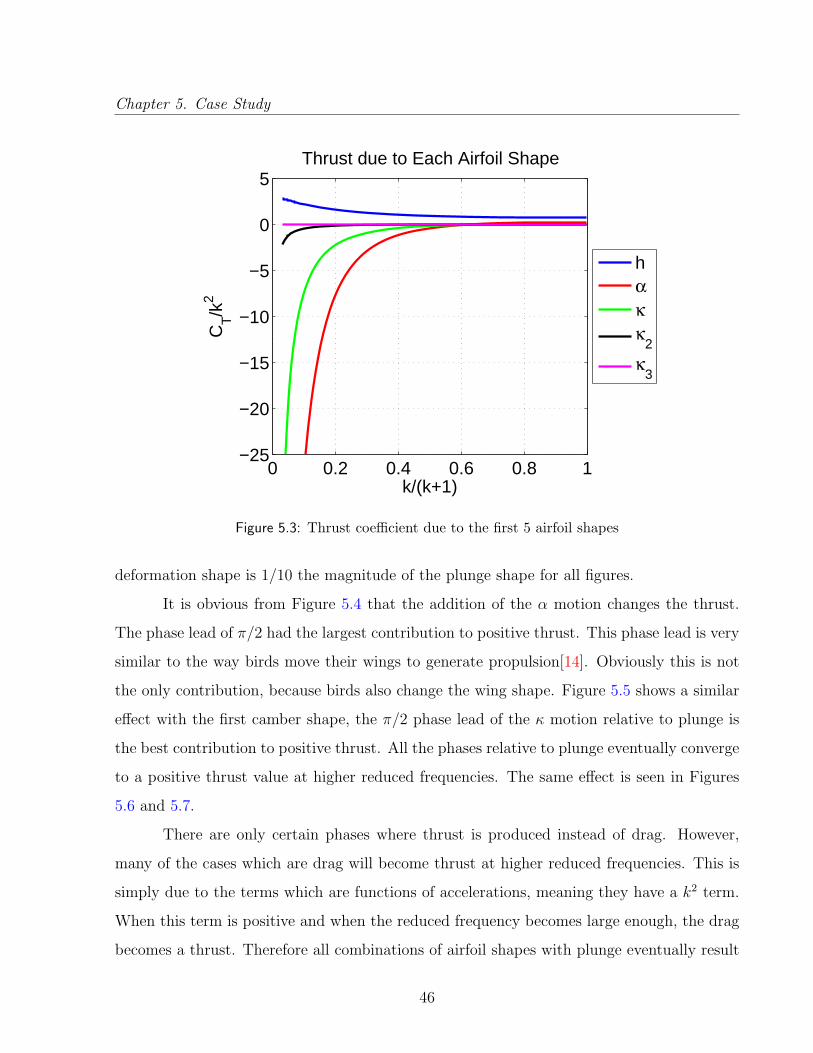
rather than go to infinity as k grows large. Figure 5.3 shows the thrust force coefficient for unit

non-dimensional displacement/deformation due to each of the first five shapes individually.

The thrust is a function of the square of the reduced frequency, and therefore the thrust

coefficient is divided by k2. The x-axis is k/(k + 1) so that values of reduced frequency

between 0 and infinity can easily be seen. The amplitude of oscillation, h, α... are set equal

to 1.

Figure 5.3 shows that the plunge shape is the only motion with significant thrust, as

shown by Garrick[2]. However, this shape along with the other shapes have cross coupling

terms which can lead to added thrust depending on the phase of the motion relative to the

plunge motion. The following four figures show combinations of plunge and the latter airfoil

shapes at different phases to show how the thrust varies. The magnitude of the additional

45


0 0.2 0.4 0.6 0.8 1−25

−20

−15

−10

−5

0

5

k/(k+1)

CT/k

2

Thrust due to Each Airfoil Shape

hακκ

2

κ3

Figure 5.3: Thrust coefficient due to the first 5 airfoil shapes

deformation shape is 1/10 the magnitude of the plunge shape for all figures.

It is obvious from Figure 5.4 that the addition of the α motion changes the thrust.

The phase lead of π/2 had the largest contribution to positive thrust. This phase lead is very

similar to the way birds move their wings to generate propulsion[14]. Obviously this is not

the only contribution, because birds also change the wing shape. Figure 5.5 shows a similar

effect with the first camber shape, the π/2 phase lead of the κ motion relative to plunge is

the best contribution to positive thrust. All the phases relative to plunge eventually converge

to a positive thrust value at higher reduced frequencies. The same effect is seen in Figures

5.6 and 5.7.

There are only certain phases where thrust is produced instead of drag. However,

many of the cases which are drag will become thrust at higher reduced frequencies. This is

simply due to the terms which are functions of accelerations, meaning they have a k2 term.

When this term is positive and when the reduced frequency becomes large enough, the drag

becomes a thrust. Therefore all combinations of airfoil shapes with plunge eventually result

46


0 0.2 0.4 0.6 0.8 1−10

−5

0

5

10

k/(k+1)

CT/k

2

Thrust Coefficient Due to h and α

hφ

α=−π/2

φα=0

φα=π/2

φα=π

Figure 5.4: Thrust coefficient due to h and α

0 0.2 0.4 0.6 0.8 1−15

−10

−5

0

5

10

15

20

k/(k+1)

CT/k

2

Thrust Coefficient Due to h and κ

hφ

κ=−π/2

φκ=0

φκ=π/2

φκ=π

Figure 5.5: Thrust coefficient due to h and κ

47


0 0.2 0.4 0.6 0.8 1−1

0

1

2

3

4

5

6

7

k/(k+1)

CT/k

2

Thrust Coefficient Due to h and κ2

hφ

κ2=−π/2

φκ2

=0

φκ2

=π/2

φκ2

=π

Figure 5.6: Thrust coefficient due to h and κ2

0 0.2 0.4 0.6 0.8 10.5

1

1.5

2

2.5

3

3.5

4

k/(k+1)

CT/k

2

Thrust Coefficient Due to h and κ3

hφ

κ3=−π/2

φκ3

=0

φκ3

=π/2

φκ3

=π

Figure 5.7: Thrust coefficient due to h and κ3

48


in thrust.

Combinations of airfoil shapes without plunge included are given in Figures 5.8

through 5.13. These airfoil shape combinations result in drag at low frequencies for every

case, and for the shape combinations without α, result in drag at all frequencies. However,

as with the flows including plunge, the combinations with α becomes positive after some

reduced frequency.

0 0.2 0.4 0.6 0.8 1−35

−30

−25

−20

−15

−10

−5

0

k/(k+1)

CT/k

2

Thrust Coefficient Due to α and κ

αφ

κ=−π/2

φκ=0

φκ=π/2

φκ=π

Figure 5.8: Thrust coefficient due to α and κ

Figures 5.8 through 5.13 show that every combination of the first five airfoil shapes

without plunge will result in a drag rather than thrust at low reduced frequency. However,

take for instance the flow consisting of h, κ2, and κ3. The combinations of h and κ2, and

h and κ3 are both large, but the combination of κ2 and κ3 is a drag which is quite small.

Therefore the combination of h, κ2 and κ3 may result in more thrust than h and κ2, and

h and κ3 alone. There is much to be done in analyzing this; these results only take into

account the magnitude of 1/10 the plunge magnitude. Figures 5.14 through 5.17 show the

combination of h, κ2 and κ3. These plots each have a constant κ2 phase relative to plunge

49


0 0.2 0.4 0.6 0.8 1−35

−30

−25

−20

−15

−10

−5

0

k/(k+1)

CT/k

2

Thrust Coefficient Due to α and κ2

αφ

κ2=−π/2

φκ2

=0

φκ2

=π/2

φκ2

=π

Figure 5.9: Thrust coefficient due to α and κ2

and varying κ3 phase.

Nearly every phase combination for the three deformations of Figures 5.14 through

5.17 results in thrust. There are several cases which did not result in thrust at very low

frequencies. Take, for instance Figure 5.14; every curve results in drag rather than thrust

at low frequencies, but becomes thrust at higher frequencies. Just like the curves for only

one more shape and plunge, the effect of the positive k2 takes over after a certain value of

k and the thrust force becomes positive. The value of reduced frequency this occurs at is

dependent on the phase angle. It makes sense that there is no curve for this case which is

always thrust because the phase of κ2 is −π/2. Figure 5.6 shows this phase angle to produce

drag at low frequencies instead of thrust.

As seen with the combinations of h and every other shape, the phase of the second

motion relative to h of π/2 always produces thrust, and it follows that the combinations of

h, κ2, and κ3 with this phase should be similar. Figure 5.16 shows this; every curve always

produces thrust when φκ2 = π/2.

50


0 0.2 0.4 0.6 0.8 1−35

−30

−25

−20

−15

−10

−5

0

k/(k+1)

CT/k

2

Thrust Coefficient Due to α and κ3

αφ

κ3=−π/2

φκ3

=0

φκ3

=π/2

φκ3

=π

Figure 5.10: Thrust coefficient due to α and κ3

0 0.2 0.4 0.6 0.8 1−10

−8

−6

−4

−2

0

k/(k+1)

CT/k

2

Thrust Coefficient Due to κ and κ2

κφ

κ2=−π/2

φκ2

=0

φκ2

=π/2

φκ2

=π

Figure 5.11: Thrust coefficient due to κ and κ2

51


0 0.2 0.4 0.6 0.8 1−10

−8

−6

−4

−2

0

k/(k+1)

CT/k

2

Thrust Coefficient Due to κ and κ2

κφ

κ2=−π/2

φκ2

=0

φκ2

=π/2

φκ2

=π

Figure 5.12: Thrust coefficient due to κ and κ3

0 0.2 0.4 0.6 0.8 1

−0.5

−0.4

−0.3

−0.2

−0.1

0

0.1

k/(k+1)

CT/k

2

Thrust Coefficient Due to κ2 and κ

3

κ2

φκ3

=−π/2

φκ3

=0

φκ3

=π/2

φκ3

=π

Figure 5.13: Thrust coefficient due to κ2 and κ3

52


0 0.2 0.4 0.6 0.8 1−2

−1

0

1

2

3

k/(k+1)

CT/k

2

Thrust Coefficient Due to h, κ2 and κ

3 (φ

κ2=−π/2)

h and κ2

φκ3

=−π/2

φκ3

=0

φκ3

=π/2

φκ3

=π

Figure 5.14: Thrust coefficient due to h, κ2 and κ3 (φκ2 = −π/2)

0 0.2 0.4 0.6 0.8 10.5

1

1.5

2

2.5

3

3.5

k/(k+1)

CT/k

2


3 (φ

κ2=0)

h and κ2

φκ3

=−π/2

φκ3

=0

φκ3

=π/2

φκ3

=π

Figure 5.15: Thrust coefficient due to h, κ2 and κ3 (φκ2 = 0)

53


0 0.2 0.4 0.6 0.8 10

2

4

6

8

k/(k+1)

CT/k

2


3 (φ

κ2=π/2)

h and κ2

φκ3

=−π/2

φκ3

=0

φκ3

=π/2

φκ3

=π

Figure 5.16: Thrust coefficient due to h, κ2 and κ3 (φκ2 = π/2)

0 0.2 0.4 0.6 0.8 10.5

1

1.5

2

2.5

3

3.5

4

k/(k+1)

CT/k

2


3 (φ

κ2=π)

h and κ2

φκ3

=−π/2

φκ3

=0

φκ3

=π/2

φκ3

=π

Figure 5.17: Thrust coefficient due to h, κ2 and κ3 (φκ2 = π)

54

Chapter 6

Conclusions and Future Work

6.1 Conclusions

The unsteady aerodynamics of deformable airfoils was addressed in this thesis. The defor-

mation of the airfoil is represented by a series of Chebychev polynomials. The aerodynamics

model was developed using potential flow aerodynamics. The model consisted of a sheet

of sources/sinks stretched along a circle. The Joukowski conformal mapping technique was

used to map the flow around the circle to the flow around a flat plate. The strength of

the sheet was determined by the no penetration boundary condition. The circulation was

modeled as a sheet of vortices extending to infinity in the wake, and a sheet on the body for

the bound circulation. The strength of the sheet was determined by the Kutta condition.

These boundary conditions were used to derive the lift, pitching moment and thrust on a

flat plate which can pitch, plunge, and deform in any shape. The key conclusions based on

a case study investigating the resulting equations are as follows.

• Theodorsen’s function reduces the magnitude of the lift due to circulation as reduced

frequency increases.

• Theodorsen’s function shifts the phase of the circulatory lift with respect to the motion

for all airfoil deformation. The magnitude of the phase shift is dependent on the reduced

55

Chapter 6. Conclusions and Future Work

frequency.

• As shown by Garrick, plunging of a flat plate always leads to thrust.

• Combinations of plunging with other displacement/deformation shapes leads to changes

in the thrust as compared to pure plunging. When the deformation leads the plunge

by π/2 there is an increase in the magnitude of the thrust as compared to plunging

only.

• The magnitude of the pitching and deformation motion relative to the plunge magni-

tude affects the thrust.

6.2 Future Work

The method derived in this thesis yields the lift force, pitching moment, and thrust for an

airfoil deforming harmonically. The derived theory is an inviscid, two dimensional theory.

Many flapping wing MAV’s will have motion outside the regime of small disturbances, and

likely have significant three dimensional effects. However, steady aerodynamics has shown

the use of thin airfoil theory to be quite helpful in conceptual design of aircraft. Therefore

it is expected that the theory developed in this thesis will be helpful in preliminary design

of flapping wing aircraft. Further, the theory will be helpful in understanding how birds and

insects generate lift and propulsion. The present theory can be used as the foundation to

develop a more advanced theory. There are numerous possibilities for other work to be done

in conjunction with this work and as extensions to this work. Several paths for future work

include the following.

• Derive the lift, thrust and pitching moment for a different set of orthogonal functions.

• Investigate the effect of mean camber and thickness by changing the location of the

Joukowski circle being mapped to a location other than the origin.

• Investigate the effect of dynamically moving the circle being mapped vertically.

56

Chapter 6. Conclusions and Future Work

• Develop methodology for optimizing the deformation shape for thrust generation (mag-

nitude and efficiency).

• Couple the unsteady aerodynamic model with membrane structural model to develop

a methodology for aeroelastic analysis of MAV wings.

• Investigate the lift, thrust and pitching moment during transient motion.

57

References

[1] Theodorsen, T., “General Theory of Aerodynamic Instability and the Mechanism of

Flutter,” NACA TR No. 496, May 1934.

[2] Garrick, I. E., “Propulsion of a Flapping and Oscillating Airfoil,” NACA TR No. 567,

May 1936.

[3] von Karman, T. and Burgers, J. M., General Aerodynamic Theory-Perfect Fluids ,

Vol. II, Julius Springer, Berlin, 1935.

[4] Katz, J. and Plotkin, A., Low-Speed Aerodynamics , Cambridge University Press, 2002.

[5] Wagner, H., “Uber die Entstehung des dynamischen Auftriebes von Tragflugeln,” Febru-

ary 1925, pp. 17–35.

[6] Garrick, I. E., “On Some Reciprical Relations in the Theory of Nonstationary Flows,”

NACA TR No. 629, March 1938.

[7] Kussner, H. G., “Zusammenfassender Bericht uber den instationaren Auftrieb von

Flugeln,” December 1936, pp. 410–424.

[8] von Karman and Sears, “Airfoil Theory for Non-Uniform Motion,” Journal of the Aero-

nautical Sciences , Vol. 5, No. 10, 1938, pp. 379–390.

[9] Sears, W. R., “Operational Methods in the Theory of Airfoils in Non-Uniform Motion,”

Journal of the Franklin Institute, Vol. 230, July 1940, pp. 95–111.

58

REFERENCES

[10] Isaacs, R., “Airfoil Theory for Flows of Variable Velocity,” Journal of the Aeronautical

Sciences , Vol. 12, No. 1, 1945, pp. 113–117.

[11] Isaacs, R., “Airfoil Theory for Rotary Wing Aircraft,” Journal of the Aeronautical Sci-

ences , Vol. 13, No. 4, 1946, pp. 218–220.

[12] Loewy, R., “A Two-Dimensional Approximation to the Unsteady Aerodynamics of Ro-

tary Wings,” Journal of the Aeronautical Sciences , Vol. 24, No. 2, February 1957, pp. 81–

92.

[13] Greenberg, J. M., “Airfoil in Sinusoidal Motion in a Pulsating Stream,” NACA TN No.

1326, June 1947.

[14] Zbikowski, R., “On aerodynamic modelling of an insect-like flapping wing in hover for

micro air vehicles,” Philosophical Transactions of the Royal Society London, Series A

(Mathematical, Physical and Engineering Sciences), Vol. 360, No. 1791, 2002/02/15,

pp. 273 – 90.

[15] Azuma, A. and Okamoto, M., “Theoretical Study of the Two-dimensional Aerodynamic

Charecteristics of Unsteady Wings,” Journal of Theoretical Biology , November 2004.

[16] Patil, M. J., “From fluttering wings to flapping flight: The energy connection,” Journal

of Aircraft , Vol. 40, No. 2, 2003, pp. 270 – 276.

[17] Peters, D. A., Hsieh, M.-C. A., and Torrero, A., “A state-space airloads theory for

flexible airfoils,” Annual Forum Proceedings - AHS International , Vol. III, Phoenix,

AZ, United states, 2006, pp. 1806 – 1823.

[18] Peters, D., “Two-dimensional incompressible unsteady airfoil theory-An overview,”

Journal of Fluids and Structures , Vol. 24, No. 3, 2008, pp. 295 – 312.

[19] Johnston, C., “Review, Extension, and Application of Unsteady Thin Airfoil Theory,”

CIMSS Report No. 04-101, Center for Intelligent Material Systems and Structures, Vir-

ginia Polytechnic Institute and State Univeristy, Blacksburg, VA, August 2004.

59

REFERENCES

[20] Glegg, S. and Devenport, W., “Unsteady loading on an airfoil of arbitrary thickness,”

Journal of Sound and Vibration, Vol. 319, No. 3-5, 2009, pp. 1252 – 70.

[21] Jones, R. T., “The Unsteady Lift of a Wing of Finite Aspect Ratio,” NACA TR No.

681, June 1939.

[22] Hernandes, F. and Soviero, P. A. D. O., “A numerical model for thin airfoils in unsteady

compressible arbitrary motion,” Journal of the Brazilian Society of Mechanical Sciences

and Engineering , Vol. 29, No. 3, 2007, pp. 253 – 261.

[23] Bisplinghoff, R., A. H. and Halfman, R., Aeroelasticity , Addison-Wesley, 1955.

60

Appendix A: Theodorsen’s Function

The complete derivation of Theodorsen’s function is given in reference [1]. This section

intends to highlight some of the aspects of the derivation and show the real and imaginary

parts used in the calculation of the average thrust force in the case study of chapter 5.

Integral forms of Bessel functions J0, J1, Y0, and Y1 derived by Theodorsen are given below

in Eq. (A.1).

−π2Y0(k) =

∞∫1

cos kx0√x2

0 − 1dx0

π

2J0(k) =

∞∫1

sin kx0√x2

0 − 1dx0

−π2Y1(k) =

∞∫1

x0 sin kx0√x2

0 − 1dx0

−π2J1(k) =

∞∫1

x0 cos kx0√x2

0 − 1dx0

(A.1)

Theodorsen’s function is rewritten in Eq. (A.2) below.

C (k) =

∫∞1

x0√x20−1

e−ikx0dx0∫∞1

x0√x20−1

e−ikx0dx0 +∫∞

11√x20−1

e−ikx0dx0

(A.2)

61

REFERENCES

Using Euler’s equation, the exponential is written in the trigonometric form.

C (k) =

∫∞1

x0 cos kx0√x20−1

dx0 − i∫∞

1x0 sin kx0√

x20−1

dx0∫∞1

x0 cos kx0√x20−1

dx0 − i∫∞

1x0 sin kx0√

x20−1

dx0 +∫∞

1cos kx0√x20−1

dx0 − i∫∞

1sin kx0√x20−1

dx0

(A.3)

Combining Eqs. (A.1) and (A.3) Theodorsen’s function is written in terms of Bessel

functions.

C (k) =−π

2J1(k) + iπ

2Y1(k)

−π2J1(k) + iπ

2Y1(k)− π

2Y0(k)− iπ

2J0(k)

=−J1(k) + iY1(k)

−(J1(k) + Y0(k)) + i(Y1(k)− J0(k))

(A.4)

Eq. (A.4) is split up into real and imaginary parts in Eq. (A.5).

C (k) = F (k) + iG(k)

F (k) =J1(k)(J1(k) + Y0(k)) + Y1(k)(Y1(k)− J0(k))

(J1(k) + Y0(k))2 + (Y1(k)− J0(k))2

G(k) = − Y1(k)Y0(k) + J1(k)J0(k)

(J1(k) + Y0(k))2 + (Y1(k)− J0(k))2

(A.5)

This form of Theodorsen’s function much more easily shows it’s effect on reducing the

circulatory lift magnitude and shifting the phase of the circulatory lift relative to the motion.

Recalling Eq. (3.42), the relationship for Theodorsen’s function can be written in terms of

Hankel functions. The numerator and first two terms of the denominator of Eq. (A.4) become

−H(2)1 (k). The last two terms of the denominator are −iH(2)

0 (k). Therefore the alternate for

of Theodorsen’s function is written as Eq. (A.6).

62

REFERENCES

C (k) =H

(2)1 (k)

H(2)1 (k) + iH

(2)0 (k)

(A.6)

Figure A.1 below shows a plot of the real and imaginary parts of Theodorsen’s function

as a function of reduced frequency.

0 10 20 30 40 500

0.1

0.2

0.3

0.4

0.5

0.6

0.7

0.8

0.9

1

1/k

Theodorsen’s Function

F(k)−G(k)

Figure A.1: Functions F and G as a function of 1/k

63

unsteady aerodynamics of deformable thin airfoils€¦ · unsteady aerodynamics of deformable thin...

Documents