unsupervised learning of object landmarks by factorized...
TRANSCRIPT

Unsupervised learning of object landmarks by factorized spatial embeddings
James Thewlis
University of Oxford
Hakan Bilen
University of Oxford
University of Edinburgh
Andrea Vedaldi
University of Oxford
Abstract
Learning automatically the structure of object categories
remains an important open problem in computer vision. In
this paper, we propose a novel unsupervised approach that
can discover and learn landmarks in object categories, thus
characterizing their structure. Our approach is based on
factorizing image deformations, as induced by a viewpoint
change or an object deformation, by learning a deep neu-
ral network that detects landmarks consistently with such
visual effects. Furthermore, we show that the learned land-
marks establish meaningful correspondences between dif-
ferent object instances in a category without having to im-
pose this requirement explicitly. We assess the method qual-
itatively on a variety of object types, natural and man-made.
We also show that our unsupervised landmarks are highly
predictive of manually-annotated landmarks in face bench-
mark datasets, and can be used to regress these with a high
degree of accuracy.
1. Introduction
The appearance of objects in images depends strongly
not only on their intrinsic properties such as shape and ma-
terial, but also on accidental factors such as viewpoint and
illumination. Thus, learning from images about objects as
intrinsic physical entities is extremely difficult, particularly
if no supervision is provided.
Despite these difficulties, the performance of object de-
tection algorithms has been rising steadily, and deep neural
networks now achieve excellent results on benchmarks such
as PASCAL VOC [17] and Microsoft COCO [39]. Still,
it is unclear whether these models conceptualise objects as
intrinsic entities. Early object detectors such as HOG [13]
and DPMs [18] were based on 2D templates applied in a
translation and scale invariant manner to images. Recent
detectors such as SSD [42] make this even more extreme
and learn different templates (filters) for different scales and
even different aspect ratios of objects. Hence, these mod-
els are likely to capture objects as image-based phenomena,
representing them as a collection of weakly-related 2D pat-
Unlabelled images
Viewpoint factorization
Learned landmarks
Figure 1. We present a novel method that can learn viewpoint in-
variant landmarks without any supervision. The method uses
a process of viewpoint factorization which learns a deep landmark
detector compatible with image deformations. It can be applied to
rigid and deformable objects and object categories.
terns.
Achieving a deeper understanding of objects requires
modeling their intrinsic viewpoint-independent structure.
Often this structure is defined manually by specifying en-
tities such as landmarks, parts, and skeletons. Given suffi-
cient manual annotations, it is possible to teach deep neural
networks and other models to recognize such structures in
images. However, the problem of learning such structures
without manual supervision remains largely open.
In this paper, we contribute a new approach to learn
viewpoint-independent representations of objects from im-
ages without manual supervision (fig. 1). We formulate this
task as a factorization problem, where the effects of image
deformations, for example arising from a viewpoint change,
are explained by the motion of a reference frame attached
to the object and independent of the viewpoint.
After describing the general principle (sec. 3.1), we in-
15916

vestigate a particular instantiation of it. In this model, the
structure of an object is expressed as a set of landmark
points (sec. 3.2) detected by a neural network. Differently
from traditional keypoint detectors, however, the network
is learned without manual supervision. Learning considers
pairs of images related by a warp and requires the detector’s
output to be equivariant with the transformation (sec. 3.3).
Transformations could be induced by real-world viewpoint
changes or object deformations, but we show that meaning-
ful landmarks can be learned even by considering random
perturbations only.
We show that this method works for individual rigid and
deformable object instances (sec. 3.1.1) as well as for object
categories (sec. 3.1.2). This only requires learning a sin-
gle neural network to detect the same set of landmarks for
images containing different object instances of a category.
While there is no explicit constraint that forces landmarks
for different instances to align, we show that, in practice,
this tends to occur automatically.
The method is tested qualitatively on a variety of differ-
ent object types, including shoes, animals, and human faces
(sec. 4). We also show that the unsupervised landmarks are
highly predictive of manually-annotated landmarks, and as
such can be used to detect these with a high degree of ac-
curacy. In this manner, our method can also be used for
unsupervised pretraining of semantic landmark detectors.
2. Related work
Flow. Matching images up to a motion-induced deforma-
tion links back to the work of Horn and Schunck [26] on
optical flow and to deep learning approaches for its compu-
tation [21, 57, 28]. Flow can also be defined semantically
rather than geometrically [40, 32, 46, 77, 76]. While our
method also establishes geometric and (indirectly) seman-
tic correspondences, it goes beyond that by learning a single
set of viewpoint independent landmarks which are valid for
all images at once.
Parts. A traditional method to describe the structure of
objects is to decompose them into their constituent parts.
Several unsupervised methods to learn parts exist, from the
constellation approach used in [19, 9, 62] to the Deformable
Parts Model (DPM) [18] and many others. More recently,
AnchorNet [48] successfully learns parts that match differ-
ent object instances as well as different object categories
using only image-level supervision; furthermore, they pro-
pose a part orthogonality constraint similar to our own.
While the concepts of landmarks and parts are similar, our
training method differs substantially from these approaches:
rather than learning parts as a byproduct of learning a (de-
formable) discriminator, our landmark points are trained to
fit geometric deformations directly.
Deformation-prediction networks. WarpNet [30] learns a
neural network that, given two images, predicts a Thin Plate
Spline (TPS [6]) that aligns them. While our landmarks
can also be seen as a representation of transformations (as
matching them between image pairs induces one), learning
such landmarks is unique to our method. The Deep De-
formation Network of [69] predicts image transformations
to refine landmarks using a “Point Transformer Network”,
but their landmarks are learned using full manual supervi-
sion, whereas our method is fully unsupervised. Very re-
cently [53] learn a neural network that also aligns two im-
ages by estimating the transformation between them, im-
plicitly learning feature extractors that could be similar to
keypoints; however, our work explicitly trains a network
to output keypoints that are equivariant to such transforma-
tions.
Landmark detection. There is an extensive literature
on landmark detectors, particularly for faces. Exam-
ples include Active Appearance Models [11], along with
subsequent improvements [44, 12] and others using tem-
plates [51] or parts [80]. Other approaches directly regress
the landmark coordinates [59, 14, 10, 52]. Deep learning
methods use cascaded CNNs [56], coarse-to-fine autoen-
coders [70], auxiliary attribute prediction [73, 74], learned
deformations [69] and LSTMs [64]. Beyond faces, there is
work on humans [65, 58], birds [55, 41, 69] and furniture
[63]. More general pose estimation including the case of
landmarks is explored in [16]. Our method can build on any
such detector architecture and can be used as a pretraining
strategy to learn landmarks with less or no supervision.
Equivariance constraint. A variant of the equivariance
constraint used by our method was proposed by [37] to learn
feature point detectors for image matching. We build on a
similar principle, but use it to learn intrinsic landmarks for
object categories instead of generic SIFT-like features with
a robust learning objective and learn to detect a set of com-
plementary landmarks rather than a single one at a time.
Unsupervised pretraining. Unsupervised pretraining has
received significant interest with the popularization of data-
hungry deep networks [5, 24, 23]. Unsupervised learn-
ing is based on training a network to solve auxiliary tasks,
for which supervision can be obtained without manual an-
notations. The most common of such tasks is to gener-
ate the data (autoencoders [7, 4, 25]); or one can remove
some information in images and train a network to recon-
struct it (denoising [60], ordering patches [15, 47], inpaint-
ing [50], analyzing motion [1, 49, 61, 20, 45], and coloriz-
ing [71, 35]). Our method can be seen in this light as trying
to undo a synthetic deformation applied to an image.
Our method is also related to unsupervised learning for
faces, such as alignment based on a face model [78], learn-
ing meaningful descriptors [67, 22], and learning a part
model [38]. Huang et al. [27] learn joint alignment of faces
using deep features, and Jaiswal et al. [29] use clustering
to discover head modes in order to refine manually-defined
landmarks in an unsupervised manner, both using genera-
5917

Figure 2. Modelling the structure of objects. Points r in the
reference space S0 (conceptually a sphere) index corresponding
points in different object instances. Given an image x, the map
Φ(r;x) detects the location q of the reference point r. The map
must be compatible with warps g of the objects. For different
views of the same (deformable) object instance, the warp g is de-
fined geometrically, whereas for object categories (as shown) it is
defined semantically.
tive principles. None of these methods learns landmarks
from scratch.
3. Method
Sec. 3.1 introduces the method of viewpoint factoriza-
tion for learning an intrinsic reference frame for object in-
stances and categories. Then, sec. 3.2 applies it to learn
object landmarks and sec. 3.3 discusses the details of the
learning formulation.
3.1. Structure from viewpoint factorization
Let S ⊂ R3 be the surface of a physical object, say a
bird, and let x : Λ → R be an image of the object, where
Λ ⊂ R2 is the image domain (fig. 2). The surface S is an in-
trinsic property of the object, independent of the particular
image x and of the corresponding viewpoint. We consider
the problem of learning a function q = ΦS(p;x) that maps
object points p ∈ S to the corresponding pixels q ∈ Λ in
the image.
We propose a new method to learn ΦS automatically
through a process of viewpoint factorization. To this end,
consider a second image x′ of the object seen from a differ-
ent viewpoint. Occlusion not withstanding, one can write
x′ ≈ x ◦ g where g : R2 → R
2 is the image warp induced
by the viewpoint change. Using the map ΦS , the warp g can
be factorised as follows:
g = ΦS(·;x′) ◦ ΦS(·;x)
−1. (1)
In other words, we can decompose the warp g : q 7→ q′ as
first finding the intrinsic object point p = Φ−1S (q;x) corre-
sponding to pixel q in image x and then finding the corre-
sponding pixel q′ = ΦS(p;x′) in image x
′.
The factorization eq. (1) is more conveniently expressed
as the following equivariance constraint:
∀p ∈ S : ΦS(p;x ◦ g) = g(ΦS(p;x)). (2)
This constraint simply states that the points p must be de-
tected in a manner which is consistent with a viewpoint
change.
In order to learn the map ΦS , we express the latter as a
deep neural network and train it to satisfy constraint (2) in
a Siamese configuration, supplying triplets (x,x′, g) to the
learning process. Note that, if we are given two views x
and x′ of the same object, the viewpoint transformation g
is often unknown. Instead of trying to recover g, inspired
by [30], we propose to synthesize transformations g at ran-
dom and use them to generate x′ from x. While this ap-
proach only uses unannotated images of the object, it can
still learn meaningful landmarks (sec. 4).1
Discussion. While learning only considers deformations of
the same image, the model still learns to bridge automat-
ically across moderately different viewpoints (see fig. 5).
However we leave very large out-of-plane rotations, which
would require to handle partial occlusions of the landmarks,
to future work.
3.1.1 Deformable objects
The method developed above extends essentially with no
modification to deformable objects. Suppose that the sur-
face S deforms between images according to isomorphisms
w : R3 → R3. We tie the shape variants wS = {w(p) :
p ∈ S} together by introducing a common reference space
S0, which we call an object frame. Barring topological
changes, we can establish isomorphisms πS mapping ref-
erence points r ∈ S0 to fixed surface points πS(r) ∈ S, in
the sense that ∀w : w(πS(r)) = πwS(r). Then, by using
the substitution Φ(r;x) = ΦS(πS(r);x), we can rewrite
the equivariance constraint (2) as
∀r ∈ S0 : Φ(r;x ◦ g) = g(Φ(r;x)). (3)
This simply states that one expects surface points to be de-
tected equivariantly with viewpoint-induced deformations
as well as with deformations of the object surface.
3.1.2 Object categories
In addition to deformable objects, our formulation can eas-
ily account for shape variations between object instances in
the same category. To do this, one simply makes the as-
sumption that all object surfaces S are isomorphic to the
same reference shape S0 (fig. 2).
Differently from the case of deformable objects, geome-
try alone does not force the mappings πS for different object
1If x and x′ are given but g is unknown, one can rewrite eq. (2) by
expressing the warp g as a function of the predicted landmarks (as the
solution of the equation ∀p : ΦS(p;x′) = gΦS(p;x)), and then by mea-
suring the alignment quality in appearance space as ‖x′−x◦g‖. However,
this approach provides a weaker supervisory signal and is somewhat more
complex to implement.
5918

instances S to be related. Nevertheless, we would like to
choose such mappings to be semantically consistent; for ex-
ample, if πS(r) is the right eye of face S, then we would like
πS′(r) to be the right eye of face S′. An important contri-
bution of this work is to show that semantically-meaningful
correspondences emerge automatically by simply sharing
the same learned mapping Φ between all object instances
in a given category. The idea is that, by learning a sin-
gle rule that detects object points consistently with defor-
mations, these points tend to align between different object
instances as this is the smoothest solution.
3.2. Landmark detection networks
In this section we instantiate concretely the method
of sec. 3.1. First, one needs to decide how to represent
the maps Φ(·;x) : S0 → Λ as the output of a neural net-
work or other computational model. Our approach is to
sample this function at a set of K discrete reference loca-
tions Φ(x) = (Φ(r1;x), . . . ,Φ(rK ;x)). In this manner, the
function Φ(x) can be thought of as detecting the location
pk = Φ(rk;x) of K object landmarks. We do not attach
particular constraints to the set of landmarks, which can be
thought of as an index set rk = k, k = 1, 2, . . . ,K.
If Φ is implemented as a neural network, one can use
any of the existing architectures for keypoint detection
(sec. 2). Most such architectures are based on estimating
score maps Ψ(x) ∈ RH×W×K , associating a score Ψ(x)uk
to each landmark rk and image location u ∈ {1, . . . , H} ×{1, . . . ,W} ⊂ R
2. The score maps can be transformed into
probability maps by using the softmax operator σ:
p(u|x, r) = σ[Ψ(x)]ur =eΨ(x)ur
∑
v eΨ(x)vr
.
Following [66], it is then possible to extract a landmark lo-
cation by using the soft argmax operator, which computes
the expected value of this density:
u∗
r = σarg[Ψ(x)]r =∑
u
u p(u|x, r) =
∑
u ueΨ(x)ur
∑
v eΨ(x)vr
.
The overall network, computing the location of the K land-
marks, can then be expressed as
Φ(x) = σarg[Ψ(x)]. (4)
Discussion. An alternative approach for representing the
maps S0 → Λ is to predict the parameters of a parametric
transformation t. Assuming that the reference set S0 ⊂ R2
is a space of continuous coordinates, the transformation t
could be an affine one [37] or a thin plate spline (TPS) [30].
This has the advantage of capturing in one step a dense set
of object points and can be used to impose smoothness on
the map.
However, using discrete landmarks is more robust and
general. For example, individual landmarks may be un-
detectable when occluded, and this model can handle this
case more easily without disrupting the estimate of the vis-
ible landmarks. Furthermore, one does not need to make
assumptions on the family of allowable transformations,
which could be difficult in general.
3.3. Learning formulation
In this section, we show how the equivariance con-
straint (3) can be used to learn Φ from examples. The idea
is to setup the learning problem as a Siamese configuration,
in which the output of Φ on two images x and x′ is assessed
for compatibility with respect to the deformation g and the
equivariance constraint (3). We can express this condition
as the loss term:
Lalign =1
K
K∑
r=1
‖Φ(x ◦ g)r − g(Φ(x)r)‖2. (5)
In the rest of the section, we discuss two extensions
to eq. (5) that allow the system to train better landmarks:
formulating the loss directly in terms of the keypoint prob-
abilities and adding a diversity term.
Probability maps loss. Equation (5) uses the soft argmax
operator in order to localise and then compare landmarks.
We show here that one can skip this step by writing a loss
directly in terms of the probability maps, which provides a
more direct and stable gradient signal. The idea is to re-
place eq. (5) with the loss term
L′
align =1
K
K∑
r=1
∑
uv
‖u− g(v)‖2p(u|x, r)p(v|x′, r) (6)
where p(u|x, r) = σ[Ψ(x)]ur and p(v|x′, r) = σ[Ψ(x′)]vrare the landmark probability maps extracted from images x
and x′.
Minimizing loss (6) has two desirable effects. First, it
encourages the two probability maps to overlap and, second,
it encourages them to be highly concentrated. In fact, the
loss is zero if, and only if, both p and q are delta functions
and if the corresponding landmark locations match up to g.
While a naive implementation of (6) requires to visit all
pairs of pixels u and v in both images, with a quadratic com-
plexity, a linear-time implementation is possible by decom-
posing the loss as:
∑
u
‖u‖2p(u|x, r) +∑
v
‖g(v)‖2p(v|x′, r)
− 2
(
∑
u
u p(u|x, r)
)⊤
·
(
∑
v
g(v)p(v|x′, r)
)
.
5919

Diversity loss. The equivariance constraint eq. (3) and its
corresponding losses eqs. (5) and (6) ensure that the net-
work learns at least one landmark aligned with image defor-
mations. However, there is nothing to prevent the network
from learning K identical copies of the same landmark.
In order to avoid this degenerate solution, we add a di-
versity loss that requires probability maps of different land-
marks to fire in different parts of the image. The most ob-
vious approach is to penalize the mutual overlap between
maps for different landmarks r and r′:
Ldiv(x) =1
K2
K∑
r=1
K∑
r′=1
∑
u
p(u|x, r)p(u|x, r′). (7)
This term is zero only if, and only if, the support of the
different probability maps is disjoint.
The disadvantage of this approach is that it is quadratic
in the number of landmarks. An alternative and more effi-
cient diversity loss is:
L′
div(x) =∑
u
(
K∑
r=1
p(u|x, r)− maxr=1,...,K
p(u|x, r)
)
.
(8)
Just like eq. (7), this loss is zero only if the support of the
distributions is disjoint. In fact the sum of probability values
at a given point u is always greater than the max unless all
but one probability are zero. Note that we can rewrite (8)
more compactly as:
L′
div(x) = K −∑
u
maxr=1,...,K
p(u|x, r).
In practice, we found it beneficial to apply the diversity loss
after downsampling (by m×m sum pooling) the probability
maps as this encourages landmarks to be extracted farther
apart. Thus we consider:
L′′
div(x) = K −∑
u
maxr=1,...,K
∑
δu
p(mu+ δu|x, r).
where δu ∈ {0, . . . ,m− 1}2.
Learning objective. The learning objective considers
triplets (xi,x′
i, gi) of images xi and x′
i related by a view-
point warp gi and optimizes:
minΨ
λR(Ψ) +1
N
N∑
i=1
(
L′
align(xi,x′
i, gi; Ψ)+
γL′′
div(xi; Ψ) + γL′′
div(x′
i; Ψ))
, (9)
where R is a regulariser (weight shrinkage for a neural net-
work). As noted before, if triplets are not available, they
can be synthesized by applying a random transformation gito an image xi to obtain x
′
i = xi ◦ g. Note that all functions
are easily differentiable for backpropagation.
4. Experiments
In this section, we first describe the implementation de-
tails (sec. 4.1) and then report both qualitative (sec. 4.2) and
quantitative (sec. 4.3) results demonstrating the power of
our unsupervised landmark learning method.
4.1. Implementation details
In all the experiments, the detector Φ contains six con-
volutional layers with 20, 48, 64, 80, 256, K filters respec-
tively, where K is the number of object landmarks. Each
convolutional layer is followed by a batch normalization
and a ReLU layer. This network is proposed in [74] for
supervised facial keypoint estimation. Differently, instead
of downsampling the feature map after each convolutional
layer, we use only one 2 × 2 max pooling layer with a
stride of 2 after the first convolutional layer (conv1). Thus,
given an input size of H ×W × 3, the network outputs anH2 × W
2 ×K feature map. We apply a spatial softmax op-
erator to the output of the last convolutional layer to obtain
K probability maps, one for each landmark.
During training, we supply a set of triplets of (xi,x′i, gi)
as input to the network. In order to generate them, given an
example image I, one can naively sample a random TPS
and warp the image accordingly. However, as the input
images are typically centered and at most very slightly ro-
tated, the learned weights can be biased towards such a set-
ting. Instead, we randomly sample two TPS transformations
(g1, g2) and consecutively warp the given image to generate
an image pair i.e. x = I ◦ g1 and x′ = x ◦ g2 (computed us-
ing inverse image warping as x ◦ (g2 ◦ g1)). The TPS warps
are parametrized as in [6] which can be decomposed into
affine and deformation parts. To render realistic and diverse
warps, we randomly sample scale, rotation angle and trans-
lation parameters within the pre-determined ranges. Exam-
ples of the transformations are shown in figs. 3 to 5.
We initialize the weights of convolutions with random
gaussian noise and optimize the objective function (eq. (9))
(weight decay λ = 5 · 10−4, γ = 500) by using Adam [33]
with an initial learning rate 10−4 until convergence, then
reduce it by one tenth until no further improvement is seen.
4.2. Qualitative results
We train our unsupervised landmarks from scratch on
three different domains: shoes (fig. 3), cat faces (fig. 4),
and faces (fig. 5), and assess them qualitatively. We train
landmark detectors on 49525 shoes from the UT Zappos50k
dataset of [68] and 8609 images from the cat heads dataset
of [72] and keep the rest for validation. Facial landmarks
are learned on the CelebA dataset [43] which contains more
than 200k celebrity images for 10k identities with 5 anno-
tated landmarks. We use the provided cropped face images,
which are roughly centered and scaled to the same size.
We train an 8 or 10 landmark network for each of the
tasks to allow for clearer visualization. In addition, we show
5920

Figure 3. Unsupervised landmarks on shoes (8 landmark network). Top: synthetic TPS deformations (original image leftmost). Bottom:
different instances. Note that landmarks are consistently detected despite the significant variation in pose, shape, materials, etc.
Figure 4. Unsupervised landmarks on cat faces (10 landmark network). Top-left quintuple: synthetic deformations (original image leftmost)
transformed by rotation (images 2,3) and TPS warps (images 4,5). Remaining examples: different instances.
n landmarks Regressor training Mean error
10 MAFL 7.95
30 MAFL 7.15
50 MAFL 6.67
10 CelebA 6.32
30 CelebA 5.76
50 CelebA 5.33Table 1. Results on MAFL test set in terms of the inter-ocular dis-
tance as in [74, 52]. For each setting, n unsupervised landmarks,
that is learned on the CelebA training set, are regressed into 5
manually-defined landmarks. The regressor is learnt on CelebA
or MAFL training set.
examples of a 30-landmark network for faces in fig. 6. In
all cases we observe that: i) landmarks are detected con-
sistently up to synthetic warps (affine or TPS) of the corre-
sponding images and that ii) as a byproduct of learning to
be consistent with such transformations, landmarks are very
consistent across different object instances as well.
4.3. Quantitative results
In this section we evaluate the performance of our unsu-
pervised landmarks quantitatively by testing how well they
Method Mean Error
TCDCN [74] 7.95
Cascaded CNN [56] 9.73
CFAN [70] 15.84
Our Method (50 points) 6.67Table 2. Comparison to state-of-the-art supervised landmark de-
tectors on MAFL.
Method Mean Error
RCPR [8] 11.6
Cascaded CNN [56] 8.97
CFAN [70] 10.94
TCDCN [74] 7.65
RAR [64] 7.23
Our Method (51 points) 10.53Table 3. Comparison to state-of-the-art supervised landmark de-
tectors on AFLW (5 pts) in terms of inter-ocular distance.
correlate with and predict manually-labelled landmarks. To
do this, we consider standard facial landmark benchmarks
containing manual annotations for semantic landmarks (e.g.
eyes, corner of the mouth, etc). We first learn a detector for
K landmarks without supervision, freeze its weights, and
5921

Figure 5. Unsupervised landmarks on CelebA faces (10 landmarks network). Top: synthetic rigid and TPS deformations (original image
leftmost). Bottom: different instances. We observe landmarks highly aligned with facial features such as the mouth corners and eyes. Note
that, being unsupervised, it needn’t prefer the centers of the eyes, but consistently localizes points on the eye boundary.
Figure 6. Regression of supervised landmarks form 30 unsupervised ones (left in each pair) on MAFL. The green dot is the predicted
annotation and a small blue dot marks the ground-truth. A failure case is shown to the right.
Supervised training images Mean Error
All (19,000) 7.15
20 8.06
10 8.49
5 9.25
1 10.82Table 4. Localization results for different number of training im-
ages from MAFL used for supervised training.
Method Mean Error (68 pts)
DRMF [2] 9.22
CFAN [70] 7.69
ESR [10] 7.58
ERT [31] 6.40
LBF [52] 6.32
CFSS [79] 5.76
cGPRT [36] 5.71
DDN [69] 5.65
TCDCN [74] 5.54
RAR [64] 4.94
Ours (50 landmarks) 9.30
Ours (50 landmarks, finetune) 7.97Table 5. Comparison to state-of-the-art supervised landmark de-
tectors on 300-W.
then use the supervised training data in the benchmark to
learn a linear regressor mapping the unsupervised landmark
to the manually defined ones. The regressor takes as input
the 2K coordinates of the unsupervised landmarks, stacks
them in a vector x ∈ R2K , and maps the latter to the corre-
sponding coordinates of the manually-defined landmarks as
y = Wx. Learning W can be seen as a fully connected
layer with no bias, and is trained similarly to the unsu-
pervised network, using our warps as data augmentation.
Note that there is no backpropagation to the unsupervised
weights, which remain fixed. W is visualized in fig. 7.
Benchmark data. We first report results on the MAFL
dataset [74], a subset of CelebA with 19k training images
and 1k test images annotated with 5 facial landmarks (cor-
ners of mouth, eyes and nose). We follow the standard eval-
uation procedure in [74] and report errors in inter-ocular
distance (IOD) in table 1. Since the MAFL test set and the
CelebA training set overlap partially, we remove the MAFL
test images from CelebA when the latter is used for training.
We also consider the more challenging 300-W
dataset [54] containing 68 landmarks, obtained by merging
and re-annotating other benchmarks. We follow [52] and
use 3148 images from AFW [80], LFPW-train [3] and
Helen-train [75] as training set, and 689 images from
IBUG, LFPW-test and Helen-test as test set.
Finally we use the AFLW [34] dataset, which contains
5922
24,386 faces from Flickr. Although it contains up to 21 an-
notated landmarks, we follow [74, 64] in only evaluating
five and testing on the same 2995 faces cropped and dis-
tributed in the MTFL set of [73]. For training we use 10,122
faces that have all five points labelled and whose images are
not in the test set.
MAFL results. First, we train the unsupervised landmarks
on the CelebA training set and learn a corresponding regres-
sor on the MAFL training set. The accuracy of the regressor
on the MAFL test data is reported in table 1 and qualitative
results are shown in fig. 6.
Regressing from K = 10, 30, 50 unsupervised land-
marks improves the results. This can be explained by
the fact that more unsupervised landmarks means a higher
chance of finding some highly correlated with the five
manually-labelled ones and thus a more robust mapping
(fig. 7). This can also increase accuracy since our land-
marks are detected with a resolution of two pixels (due to
the downsampling in the network). Table 2 compares these
results to state-of-the-art fully supervised landmark local-
ization methods. Encouragingly, our best regressor outper-
forms the supervised methods (6.67 error rate vs 7.95 of
TCDCN [74]). This shows that our unsupervised training
method is indeed able to find meaningful landmarks.
Next, in Table 4 we assess how many manual landmark
annotations are required to learn the regressor. We consider
the problem of regressing from K = 30 unsupervised land-
marks and we observe that the regressor performs well even
if only 10 or 20 images are considered (errors 8.5 and 8.06).
By comparison, using all 19,000 training samples reduces
the error to 7.15, which shows that most of the required in-
formation is contained in the unsupervised landmarks from
the outset. This indicates that our method is very effec-
tive for unsupervised pretraining of manually annotated
landmarks as well, and can be used to learn good semantic
landmarks with few annotations.
300-W results. We use our best performing model, the 50
point network, trained unsupervised on CelebA, and report
results in table 5 for two settings. In the first one, the un-
supervised landmarks are learned on CelebA and only the
regressor is learned on the 300-W training set; we obtain an
error of 9.30. In the second setting, the unsupervised de-
tector is fine-tuned (also without supervision) on the 300-W
data to adapt the features to the target dataset. The fine-
tuning lowers the error to 7.97 and yields a comparable
result with the state-of-the-art supervised methods. This
shows another strength of our method: our unsupervised
learner can be used to adapt an existing network to new
datasets, also without using labels.
AFLW results. Due to tighter face crops, we adapt our 50-
landmark CelebA network, fine-tuning it first on similarly
cropped CelebA images and then on the AFLW training
set. The adapted network has 51 landmarks. We compare
against other methods in table 3. Once more, landmarks
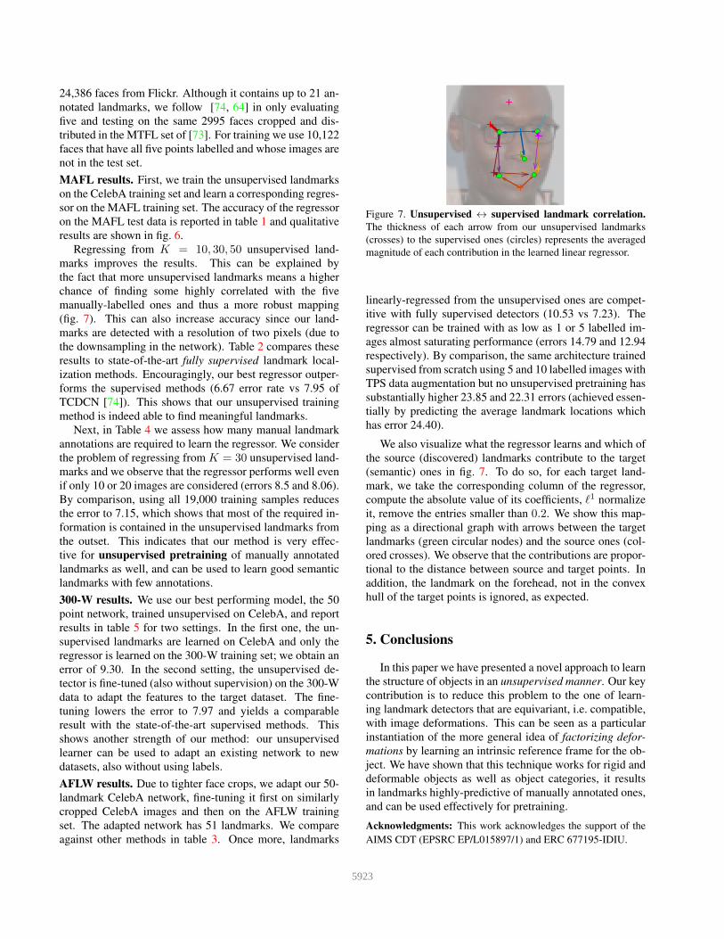
Figure 7. Unsupervised ↔ supervised landmark correlation.
The thickness of each arrow from our unsupervised landmarks
(crosses) to the supervised ones (circles) represents the averaged
magnitude of each contribution in the learned linear regressor.
linearly-regressed from the unsupervised ones are compet-
itive with fully supervised detectors (10.53 vs 7.23). The
regressor can be trained with as low as 1 or 5 labelled im-
ages almost saturating performance (errors 14.79 and 12.94
respectively). By comparison, the same architecture trained
supervised from scratch using 5 and 10 labelled images with
TPS data augmentation but no unsupervised pretraining has
substantially higher 23.85 and 22.31 errors (achieved essen-
tially by predicting the average landmark locations which
has error 24.40).
We also visualize what the regressor learns and which of
the source (discovered) landmarks contribute to the target
(semantic) ones in fig. 7. To do so, for each target land-
mark, we take the corresponding column of the regressor,
compute the absolute value of its coefficients, ℓ1 normalize
it, remove the entries smaller than 0.2. We show this map-
ping as a directional graph with arrows between the target
landmarks (green circular nodes) and the source ones (col-
ored crosses). We observe that the contributions are propor-
tional to the distance between source and target points. In
addition, the landmark on the forehead, not in the convex
hull of the target points is ignored, as expected.
5. Conclusions
In this paper we have presented a novel approach to learn
the structure of objects in an unsupervised manner. Our key
contribution is to reduce this problem to the one of learn-
ing landmark detectors that are equivariant, i.e. compatible,
with image deformations. This can be seen as a particular
instantiation of the more general idea of factorizing defor-
mations by learning an intrinsic reference frame for the ob-
ject. We have shown that this technique works for rigid and
deformable objects as well as object categories, it results
in landmarks highly-predictive of manually annotated ones,
and can be used effectively for pretraining.
Acknowledgments: This work acknowledges the support of the
AIMS CDT (EPSRC EP/L015897/1) and ERC 677195-IDIU.
5923

References
[1] P. Agrawal, J. Carreira, and J. Malik. Learning to see by
moving. In Proc. ICCV, 2015. 2
[2] A. Asthana, S. Zafeiriou, S. Cheng, and M. Pantic. Robust
discriminative response map fitting with constrained local
models. In Proc. CVPR, 2013. 7
[3] P. N. Belhumeur, D. W. Jacobs, D. J. Kriegman, and N. Ku-
mar. Localizing parts of faces using a consensus of exem-
plars. PAMI, 2013. 7
[4] Y. Bengio. Learning deep architectures for AI. Foundations
and trends in Machine Learning, 2009. 2
[5] Y. Bengio, A. Courville, and P. Vincent. Representation
learning: A review and new perspectives. In PAMI, 2013.
2
[6] F. L. Bookstein. Principal Warps: Thin-Plate Splines and the
Decomposition of Deformations. PAMI, 1989. 2, 5
[7] H. Bourlard and Y. Kamp. Auto-Association by Multilayer
Perceptrons and Singular Value Decomposition. Biological
Cybernetics, 1988. 2
[8] X. P. Burgos-Artizzu, P. Perona, and P. Dollar. Robust face
landmark estimation under occlusion-supp. mat. In Proc.
ICCV, 2013. 6
[9] M. C. Burl, M. Weber, and P. Perona. A probabilistic
approach to object recognition using local photometry and
global geometry. In Proc. ECCV, 1998. 2
[10] X. Cao, Y. Wei, F. Wen, and J. Sun. Face Alignment by
Explicit Shape Regression. IJCV, 2014. 2, 7
[11] T. Cootes, G. Edwards, and C. Taylor. Active Appearance
Models. Proc. ICCV, 1998. 2
[12] D. Cristinacce and T. Cootes. Automatic feature localisation
with constrained local models. Pattern Recognition, 2008. 2
[13] N. Dalal and B. Triggs. Histograms of Oriented Gradients
for Human Detection. In Proc. CVPR, 2005. 1
[14] M. Dantone, J. Gall, G. Fanelli, and L. Van Gool. Real-time
facial feature detection using conditional regression forests.
In Proc. CVPR, 2012. 2
[15] C. Doersch, A. Gupta, and A. A. Efros. Unsupervised Vi-
sual Representation Learning by Context Prediction. In Proc.
ICCV, 2015. 2
[16] P. Dollar, P. Welinder, and P. Perona. Cascaded pose regres-
sion. In Proc. CVPR, 2010. 2
[17] M. Everingham, L. Van Gool, C. K. Williams, J. Winn, and
A. Zisserman. The Pascal Visual Object Classes (VOC)
Challenge. IJCV, 88(2), 2010. 1
[18] P. F. Felzenszwalb, R. B. Girshick, D. McAllester, and D. Ra-
manan. Object Detection with Discriminatively Trained Part
Based Models. PAMI, 2010. 1, 2
[19] R. Fergus, P. Perona, and A. Zisserman. Object class recog-
nition by unsupervised scale-invariant learning. In Proc.
CVPR, 2003. 2
[20] B. Fernando, H. Bilen, E. Gavves, and S. Gould. Self-
supervised video representation learning with odd-one-out
networks. In Proc. CVPR, 2017. 2
[21] P. Fischer, A. Dosovitskiy, E. Ilg, P. Hausser, C. Hazrba,
V. Golkov, P. van der Smagt, D. Cremers, and T. Brox.
FlowNet: Learning Optical Flow with Convolutional Net-
works. In Proc. ICCV, 2015. 2
[22] M. K. Fleming and G. W. Cottrell. Categorization of faces
using unsupervised feature extraction. In International Joint
Conference on Neural Networks, 1990. 2
[23] I. Goodfellow, Y. Bengio, and A. Courville. Deep Learning.
MIT Press, 2016. http://www.deeplearningbook.
org. 2
[24] G. E. Hinton, S. Osindero, and Y. W. Teh. A fast learning
algorithm for deep belief nets. Neural computation, 2006. 2
[25] G. E. Hinton and R. R. Salakhutdinov. Reducing the Dimen-
sionality of Data with Neural Networks. Science, 2006. 2
[26] B. K. Horn and B. G. Schunck. Determining optical flow.
Artificial Intelligence, 1981. 2
[27] G. Huang, M. Mattar, H. Lee, and E. G. Learned-Miller.
Learning to align from scratch. In Proc. NIPS, 2012. 2
[28] E. Ilg, N. Mayer, T. Saikia, M. Keuper, A. Dosovitskiy, and
T. Brox. FlowNet 2.0: Evolution of Optical Flow Estimation
with Deep Networks. In Proc. CVPR, 2017. 2
[29] S. Jaiswal, T. R. Almaev, and M. F. Valstar. Guided unsu-
pervised learning of mode specific models for facial point
detection in the wild. In ICCV Workshops, 2013. 2
[30] A. Kanazawa, D. W. Jacobs, and M. Chandraker. WarpNet:
Weakly supervised matching for single-view reconstruction.
In Proc. CVPR, 2016. 2, 3, 4
[31] V. Kazemi and J. Sullivan. One Millisecond Face Alignment
with an Ensemble of Regression Trees. In Proc. CVPR, 2014.
7
[32] I. Kemelmacher-Shlizerman and S. M. Seitz. Collection
flow. In Proc. CVPR, 2012. 2
[33] D. Kingma and J. Ba. Adam: A method for stochastic opti-
mization. In Proc. ICLR, 2015. 5
[34] M. Koestinger, P. Wohlhart, P. M. Roth, and H. Bischof. An-
notated facial landmarks in the wild: A large-scale, real-
world database for facial landmark localization. In First
IEEE International Workshop on Benchmarking Facial Im-
age Analysis Technologies, 2011. 7
[35] G. Larsson, M. Maire, and G. Shakhnarovich. Learning
representations for automatic colorization. In Proc. ECCV,
2016. 2
[36] D. Lee, H. Park, and C. D. Yoo. Face alignment using cas-
cade Gaussian process regression trees. In Proc. CVPR,
2015. 7
[37] K. Lenc and A. Vedaldi. Learning covariant feature detec-
tors. In ECCV Workshop on Geometry Meets Deep Learning,
2016. 2, 4
[38] H. Li, G. Hua, Z. Lin, J. Brandt, and J. Yang. Probabilistic
elastic part model for unsupervised face detector adaptation.
In Proc. ICCV, 2013. 2
[39] T.-Y. Lin, M. Maire, S. Belongie, J. Hays, P. Perona, D. Ra-
manan, P. Dollar, and C. L. Zitnick. Microsoft coco: Com-
mon objects in context. In Proc. ECCV, 2014. 1
[40] C. Liu, J. Yuen, and A. Torralba. SIFT Flow: Dense corre-
spondence across scenes and its applications. PAMI, 2011.
2
[41] J. Liu and P. N. Belhumeur. Bird part localization using
exemplar-based models with enforced pose and subcategory
consistency. Proc. ICCV, 2013. 2
[42] W. Liu, D. Anguelov, D. Erhan, C. Szegedy, S. Reed, C.-Y.
Fu, and A. C. Berg. SSD: Single shot multibox detector. In
Proc. ECCV, 2016. 1
5924

[43] Z. Liu, P. Luo, X. Wang, and X. Tang. Deep learning face
attributes in the wild. In Proc. ICCV, 2015. 5
[44] I. Matthews and S. Baker. Active Appearance Models Revis-
ited. IJCV, 2004. 2
[45] I. Misra, C. L. Zitnick, and M. Hebert. Shuffle and learn:
unsupervised learning using temporal order verification. In
Proc. ECCV, 2016. 2
[46] H. Mobahi, C. Liu, and W. T. Freeman. A Composi-
tional Model for Low-Dimensional Image Set Representa-
tion. Proc. CVPR, 2014. 2
[47] M. Noroozi and P. Favaro. Unsupervised learning of visual
representations by solving jigsaw puzzles. In Proc. ECCV,
2016. 2
[48] D. Novotny, D. Larlus, and A. Vedaldi. Anchornet: A weakly
supervised network to learn geometry-sensitive features for
semantic matching. In Proc. CVPR, 2017. 2
[49] D. Pathak, R. Girshick, P. Dollar, T. Darrell, and B. Hariha-
ran. Learning Features by Watching Objects Move. In Proc.
CVPR, 2017. 2
[50] D. Pathak, P. Krahenbuhl, J. Donahue, T. Darrell, and A. A.
Efros. Context Encoders: Feature Learning by Inpainting. In
Proc. CVPR, 2016. 2
[51] M. Pedersoli, T. Tuytelaars, and L. Van Gool. Using a de-
formation field model for localizing faces and facial points
under weak supervision. In Proc. CVPR, 2014. 2
[52] S. Ren, X. Cao, Y. Wei, and J. Sun. Face alignment at 3000
FPS via regressing local binary features. In Proc. CVPR,
2014. 2, 6, 7
[53] I. Rocco, R. Arandjelovic, and J. Sivic. Convolutional neu-
ral network architecture for geometric matching. In Proc.
CVPR, 2017. 2
[54] C. Sagonas, E. Antonakos, G. Tzimiropoulos, S. Zafeiriou,
and M. Pantic. 300 faces in-the-wild challenge: Database
and results. Image and Vision Computing, 47, 2016. 7
[55] K. J. Shih, A. Mallya, S. Singh, and D. Hoiem. Part Lo-
calization using Multi-Proposal Consensus for Fine-Grained
Categorization. In Proc. BMVC, 2015. 2
[56] Y. Sun, X. Wang, and X. Tang. Deep convolutional network
cascade for facial point detection. In Proc. CVPR, 2013. 2,
6
[57] J. Thewlis, S. Zheng, P. H. S. Torr, and A. Vedaldi. Fully-
Trainable Deep Matching. In Proc. BMVC, 2016. 2
[58] A. Toshev and C. Szegedy. DeepPose: Human pose estima-
tion via deep neural networks. Proc. CVPR, 2014. 2
[59] M. Valstar, B. Martinez, X. Binefa, and M. Pantic. Facial
point detection using boosted regression and graph models.
In Proc. CVPR, 2010. 2
[60] P. Vincent, H. Larochelle, Y. Bengio, and P.-A. Manzagol.
Extracting and composing robust features with denoising au-
toencoders. In Proc. ICML, 2008. 2
[61] X. Wang and A. Gupta. Unsupervised Learning of Visual
Representations Using Videos. Proc. ICCV, 2015. 2
[62] M. Weber, M. Welling, and P. Perona. Towards automatic
discovery of object categories. In Proc. CVPR, 2000. 2
[63] J. Wu, T. Xue, J. J. Lim, Y. Tian, J. B. Tenenbaum, A. Tor-
ralba, and W. T. Freeman. Single Image 3D Interpreter Net-
work. In Proc. ECCV, 2016. 2
[64] S. Xiao, J. Feng, J. Xing, H. Lai, S. Yan, and A. Kassim.
Robust Facial Landmark Detection via Recurrent Attentive-
Refinement Networks. In Proc. ECCV, 2016. 2, 6, 7, 8
[65] Y. Yang and D. Ramanan. Articulated pose estimation with
flexible mixtures-of-parts. Proc. CVPR, 2011. 2
[66] K. M. Yi, E. Trulls, V. Lepetit, and P. Fua. LIFT: Learned
invariant feature transform. Proc. ECCV, 2016. 4
[67] J. Ylioinas, J. Kannala, A. Hadid, and M. Pietikainen. Unsu-
pervised learning of overcomplete face descriptors. In CVPR
Workshops, 2015. 2
[68] A. Yu and K. Grauman. Fine-Grained Visual Comparisons
with Local Learning. In Proc. CVPR, 2014. 5
[69] X. Yu, F. Zhou, and M. Chandraker. Deep Deformation
Network for Object Landmark Localization. In B. Leibe,
J. Matas, N. Sebe, and M. Welling, editors, Proc. ECCV,
Cham, 2016. 2, 7
[70] J. Zhang, S. Shan, M. Kan, and X. Chen. Coarse-to-fine
auto-encoder networks (cfan) for real-time face alignment.
In Proc. ECCV, 2014. 2, 6, 7
[71] R. Zhang, P. Isola, and A. A. Efros. Colorful Image Col-
orization. In Proc. ECCV, 2016. 2
[72] W. Zhang, J. Sun, and X. Tang. Cat head detection - How
to effectively exploit shape and texture features. In Proc.
ECCV, 2008. 5
[73] Z. Zhang, P. Luo, C. C. Loy, and X. Tang. Facial landmark
detection by deep multi-task learning. In Proc. ECCV, 2014.
2, 8
[74] Z. Zhang, P. Luo, C. C. Loy, and X. Tang. Learning
Deep Representation for Face Alignment with Auxiliary At-
tributes. PAMI, 2016. 2, 5, 6, 7, 8
[75] E. Zhou, H. Fan, Z. Cao, Y. Jiang, and Q. Yin. Extensive fa-
cial landmark localization with coarse-to-fine convolutional
network cascade. In ICCV Workshops, 2013. 7
[76] T. Zhou, P. Krahenbuhl, M. Aubry, Q. Huang, and A. A.
Efros. Learning Dense Correspondences via 3D-guided Cy-
cle Consistency. In Proc. CVPR, 2016. 2
[77] T. Zhou, Y. J. Lee, S. X. Yu, and A. A. Efros. FlowWeb:
Joint image set alignment by weaving consistent, pixel-wise
correspondences. In Proc. CVPR, 2015. 2
[78] J. Zhu, L. Van Gool, and S. C. Hoi. Unsupervised face align-
ment by robust nonrigid mapping. In Proc. ICCV, 2009. 2
[79] S. Zhu, C. Li, C. C. Loy, and X. Tang. Face alignment by
coarse-to-fine shape searching. In Proc. CVPR, 2015. 7
[80] X. Zhu and D. Ramanan. Face detection, pose estimation,
and landmark localization in the wild. In Proc. CVPR, 2012.
2, 7
5925