Cracking clay soils Shallow water table

High rainfall

Low rainfall Coarse, sandy soils

Low rainfall Soils contain hardpan

Update of the California Vulnerability Soil Analysis forMovement of Pesticides to Ground Water: October 14, 1999

ByJohn Troiano, Frank Spurlock, and Joe Marade

STATE OF CALIFORNIAEnvironmental Protection Agency

Department of Pesticide RegulationEnvironmental Monitoring and Assessment Program

Environmental Hazards Assessment Program830 K Street, Room 200, Sacramento, Ca 95814 -3510

EH 00-05

i

Abstract

The CALVUL approach to determining spatial vulnerability to ground watercontamination has been previously described (Troiano et al., 1994; Troiano et al. 1997;Troiano et al., 1999). CALVUL is an empirical approach because it attempts to i dentifysimilar geographic features amongst sections of land where pesticide residues have beenfound in ground water. Two unique features of this approach are: 1) that no a prioridetermination is made regarding the pathway for pesticide movement to ground water; and2) that no relative scale of vulnerability is derived between land areas. This report describesa revision in the clustering analysis of soil data. The revision was conducted because thenumber of sections with pesticide detections had appr oximately doubled since the initialdevelopment of the CALVUL approach. All of the sections used for this revisionoriginated from DPR investigations which assured that sampled wells had met all aspectsof a non-point source determination, especially with respect to visual inspection of wellsites. In addition, the soil data tables originally obtained from the National ResourceConservation Service (NRCS) had been updated. The results of this analysis were verysimilar to the initial clustering analysis. Variables that were important in discriminatingclusters were permeability, shrink -swell potential, presence of a hardpan soil layer, andpresence of an annual water table. Soil texture in the initial analysis was reflected invalues for the No 200 sieve. In this revision, soil texture was indicated by thecombination of permeability and shrink -swell potential. Coarse soils were characterizedby high permeability values and no shrink -swell potential whereas clayey soils werecharacterized by very low permeability values and high shrink -swell potential. Theseobservations were compared to the No200 sieve sizes to validate this observation.Although this revision indicated a greater number of clusters, there was bettercorrespondence to general soil map s. The addition of water table as a cluster variableprovided greater separation primarily between clayey soils. Presence of a water tablecould be an important variable in the development of mitigation measures and it is one ofthe observations that require further investiation.

ii

Acknowledgements

We gratefully acknowledge all the hard work that forms the foundation of this currentstudy, and we thank all the personal in the Environmental Hazards and AssessmentProgram of the California Depa rtment of Pesticide Regulation who have worked on themany studies upon which these data are drawn.

iii

Table of Contents

Abstract ……………….……….………………………………………….. I

Acknowldgements ………………………………………………………… ii

Table of contents …………………………………………………………. iii

List of Tables ………….…………………………………………………. iv

List of Figures …………….………………………………………………. v

Introduction ……………………………………………………………….. 1Description of Statistical Methodology …………..………………….. 3Incorporation of Additional Geographical Information ……… ……. 5Testing an Application of the Vulnerability Classification ……….… 5Revision of the soil Classification and Further Application ………... 5

Materials and Methods ……………………………………………………. 6Determination of Known Contaminated Sections ………..………….. 6Statistical Analysis ………….………………………………………….. 8

Data Preparation ………..…………………………………………. 8Cluster Analysis ……………………………………………………. 10Profiling Algorithm ………………………………………………… 10

Results and Discussion ………….…………………………………………. 11Stepwise Clustering of Soil Variables ………………………………… 11

Step 1 ………….…………………………………………………….. 14Step 2 …………………….………………………………………….. 14Step 3 ……………………………….……………………………….. 14Setp 4 ………………………………………….…………………….. 20

Profiling Algorithm ……………………………………………………. 20Comparison of CALVUL Sectional Estimates withDigitized Soil Data …………..………………………………………….. 22Application of the CALVUL Approach to California’sGround Water Protection Program ……….………………………….. 27

Summary …………….……………………………………………………... 29

References …………………………..……………………………………… 31

Appendix A -Computer Programs ………….……………………………. A-1

Appendix B - Statistical Results …………...………….………………….. B-1(Appendix A and B available upon request)

iv

List of Tables

Table 1. Active ingredients detected in California w ell sampling investigations anddetermined to be derived from non -point source applications. ………………… 7

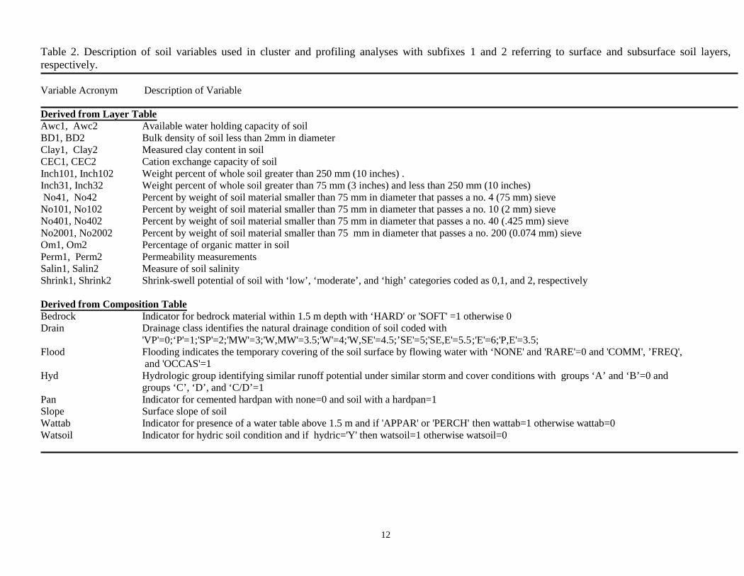
Table 2. Description of soil variables used in cluster and profiling analyses withsubfixes 1 and 2 referring to surface and subsurface soil layers, res pectively. … 12

Table 3. Correlation matrix for soil variables. At n=465, a Pearson correlationcoeffiecient of 0.13 is significant at p=0.01 so coefficients of 0.75 or greater areunderlined to illustrate trends in data. Acronyms are defined in Table 1 . ….... 13

Table 4. Significant stepwise results for clustering of soil variables. ……..…… 15

Table 5. Statistics for results of clustering analysis at each step. ……………… 16 -17

Table 6. Descriptive comparision of cluster formation between Average andCentroid clustering results at the 19 cluster solution. ………….……………… 21

v

List of Figures

Figure 1. Areas where pesticide residues have been detected in California due tonon-point source applications. ………………………………………………… 4

Figure 2. a) Plot of sectional estimates for permeability (Perm1) vs No 200 sieve(No2001) of the surface layer; b) sections estimates for shrink -swell potential(Shrink1) vs No2001. ……….………………………………………………….. 18

Figure 3. a) Plot of sectional estimates for permeability (Perm1) vs clay content(Clay1) of the surface layer; b) sections estimates for shrink -swell potential(Shrink1) vs Clay1. ……………………………………………… ……………. 19

Figure 4. Plot of the first 2 canonical variates obtained from a CanonicalDiscriminant Analysis of the output from step4 clustering by the average method.Numbers in circles are clusters as indicated in Table 6. …………………….. 23

Figure 5. Map of all CALVUL clusters characterized in Fresno and TulareCounties. ………………………………………………………………………. 24

Figure 6. Overlay of CALVUL Model estimates for sections characterized as runoffon NRCS Central Tulare County Soil Series 660 with pan soils. ………….. 25

Figure 7. Estimates of percentage of hardpan soils in a section compared betweenCALVUL and digitized NRCS soil data. S olid line is trend line and dashed line isthe the 1:1 fit. ……………………………………………………….………….. 26

Figure 8. Sections in Fresno and Tulare Counties characterized as having pan orcoarse soils, a depth to ground water of 70 feet or less from the surface, andpesticide detections. ………………………………………………….………….. 28

Figure 9. Map of all CALVUL clusters characterized in Glenn County. …… 30

1

Update of the California Vulnerability Soil Analysis forMovement of Pesticides to Ground Water

October 14, 1999

John Troiano, Frank Spurlock, and Joey Marade

Environmental Monitoring and Pest Management BranchCalifornia Department of Pesticide Regulation

830 K Street, Room 200Sacramento, CA., 95814-3510

*Corresponding author (jtroiano@cdpr.ca.gov)

Introduction

The reasons for developing a model that identifies areas of land that are vulnerable toground water contamination are:

1. To increase the efficiency of well monitoring studies . One mandated goal of wellstudies conducted by the Department of Pesticide Regulation (D PR) is to detectresidues for active ingredients that have not yet been detected in California’s groundwater (Connelly, 1986). Identification of areas with a higher probability of detectionshould focus monitoring activities and expedite the detection of new residues.

2. To delineate areas where mitigation measures should be implemented . A strength ofusing a Geographical Information System (GIS) approach is the production of mapsthat identify areas of land with similar geographic features. If geographic featurescan be related to higher probabilities of pesticide detection in well water, thenmitigation measures could be implemented within delineated areas.

3. To aid in the design and development of mitigation measures . One further steptaken in a GIS approach is to relate geographic features to the processes by whichpesticide residues move from sites of application to ground water. Practicalsignificance can then be assigned to important geographic features becausemanagement practices could be tailored to the delineated areas. Conversely, studiescould be designed to determine processes of ground water contamination in areaswhere further study is needed to describe pathways for movement of residues intoground water.

4. To fulfill programmatic mandates. The U.S. EPA is developing a process forincreased regulation of pesticides that have contaminated ground water. States willbe required to develop Pesticide Management Plans (PMPs) for pesticides ofconcern. One prong of the plan is the development of statewide vulnerabilityassessments. The California Vulnerability approach (CALVUL) is proposed tofulfill this requirement.

The CALVUL approach to determining spatial vulnerability to ground watercontamination has been previously described (Troiano et al., 1994; Troiano et al. 1997;Troiano et al., 1999). CALVUL is an empirical approach because it attempts to identifysimilar geographic features amongst sections of land where pesticide residues have been

2

found in ground water. Two unique features of this approach are: 1) that no a prioridetermination is made regarding the pathway for pesticide movement to ground water; and2) that no relative scale of vulnerability is derived between land areas. Most other methodsfocus on delineating land areas where pesticides would leach to groundwater as a resultof simple percolation of water from the land surface (National Research Council, 1993).Well sampling studies have been conducted to test spatial indices of vulnerability derivedfrom models based solely on leaching potential (U.S. Environmental Protection Agency,1992; Balu and Paulsen, 1991; Holden et al., 1992, Kalinski et al., 1994; Roux et al.,1991). Pesticide residues in these studies were detected in wells located in areasidentified as relatively invulnerable. This result reinforced our observation thatmovement of pesticide residues to ground water occurred by multiple pathways,depending on soil, climatic and agronomic factors. In California, pesticide residues hadbeen detected in coarse-textured soil areas on the eastern side of Southern San JoaquinValley and inland in Southern California (Figure 1.). Leaching with simple percolation isa likely mechanism for pesticide movement to ground water in this area. In contrast,residues have also been detected in areas where leaching was less likely such as in thefine-textured clay soils in the Sacramento Valley. Climatic conditions in areas withdetections also vary from relatively dry areas at less than 10 inches annual rainfall togreater than 60 inches of annual rainfall (Figure 1).

In addition to leaching, other potential pathways include: movement of surface water intoagricultural drainage wells (Braun and Hawkins, 1991; Roux et al., 1991); movement ofwater into Karst formations (Hallberg, 1989); or movement of water through cracks inclay soils (Graham et al. , 1992). Recently, measurement and modeling the movement ofresidues in macropore flow has gained more attention (Bergstrom et al., 1991; Chen etal., 1993).

Owing to the uncertainty in determining the exact process of pesticide movement toground water, we decided to use an empirical approach for the spatial identification ofareas that are vulnerable to ground water contamination. The first step in the CALVULmodeling approach was to identify sections of land where pesticide residues had beendetected in ground water as a result of non -point source agricultural applications. Datafor contaminated wells were obtained from the Well Inventory Data Base that ismaintained by DPR (Maes et al., 1992). Sections of land were designated as knowncontaminated (KC) sections where residues had been detected and attributed to non -pointsource agricultural applications. Sections are one -square-mile areas of land as described bythe USGS Public Land Survey (Davis and Foote, 1966). A section was chosen as thesmallest geographical unit because it was also the smallest geographical reference for otherdatabases supported at that time by the DPR such as pesticide use reporting and the WellInventory Data Base.

A non-point source determination for detection of a pesticide residue in well water is madewhen 3 conditions are fulfilled.1. Observation of well construction and pesticide storage and handling around a well rules

out potential point sources,2. Non-point source use of the pesticide in the area near the well is indicated,

3

3. Residues are measured in more than 1 well within a 1 square -mile area surrounding theoriginal detection.

Although most non-point source determinations had been conducted by DPR staff, datareported by the California Department of Health Services (DHS) were from municipalsources, as compared to predominantly domestic, rural wells sampled in DPR studies. Also,many DHS data are for pesticides no longer registere d for use in California, i.e. DBCP, 1,2-D, and EDB. Many wells sampled by DHS were determined as non -point source withoutinspection because municipal wells have a high construction standard, use of many reportedpesticides were previously suspended and c onsequently no longer regulated by DPR, andthe integrity of the chemical analysis was high because of regulatory consequences.

Description of Statistical MethodologyBased on the smallest spatial scale as possible, s tatistical clustering methods were used toidentify groups of KC sections using predominant climatic and edaphic features (Troianoet al., 1994). The following discussion focuses on the use of soil variables in the clusteranalysis. A forward stepwise cluster selection procedure was develo ped as based on asuggestion by Fowlkes et al., (1988). In the first step, a cluster analysis was conductedfor each separate variable and the single best variable that formed clusters was identified.In the second step, the single best variable was test ed in combination with the rest of thevariables and the best clustering pair of variables identified. Variables that were highlycorrelated, at a Pearson Correlation Coefficient 75%, with chosen variables wereeliminated from subsequent steps because h igh correlation between variables tends toinflate statistical measures used to test the performance of the cluster analysis(Aldenderfer and Blashfield, 1984). The stepwise process was repeated until there wasno improvement in the statistical criteria u sed to assess the clustering solution. Statisticsused to assess cluster formation were the Cubic Clustering Criterion (CCC), the Pseudo -Fand Pseudo-t2 statistics. Comparison of the absolute value of the CCC both within andbetween steps was used as the primary indicator for improvement in cluster identificationin subsequent steps (SAS Institute Inc., 1983; SAS Institute Inc., 1988).

The geographical significance of the statistical clusters was investigated by plotting thelocation of the sections that formed each cluster. The clusters did indeed distinguish landareas, providing a statistical reflection of the soil distribution described in Figure 1. Inorder to apply the results to other geographic areas, a classification algorithm wasdeveloped based on the results of the clustering procedure (Troiano et al., 1994). Thealgorithm was used to classify other sections that lacked pesticide detection or wellsampling data into one of the five KC soil clusters or, alternatively, into a not -classifiedcategory. At first, the algorithm was based on a Principal Components Analysis (PCA)applied to the results of the clustering analysis. The ability of the classification procedureto determine sections with higher probability of detection was tested in a well samplingstudy conducted in Fresno and Tulare Counties (Troiano et al., 1997). Wells weresampled in sections of land that had not been previously sampled but that were identifiedas a member of one of the prevalent vulnerable soil clusters. The ra te of pesticidedetection in those sections was 43%. This rate was considered successful when

4

5

compared to results from other surveys that used a similar sampling design of one wellper targeted area. This result, however, was dependent on the method used to generatethe profiles, whereby a classification algorithm based on Canonical DiscriminateAnalysis (CDA) appeared more accurate in determining cluster membership than thePCA based algorithm. CDA analysis was suggested by Professor Dallas Johnson(personal communication, Statistics Department, University of Kansas) who is also aninstructor for a mulitivariate statistics course given through the Institute for ProfessionalEducation, Arlington Virginia. Since the PCA -based algorithm had been develo ped adhoc, the CDA methodology was chosen because it was a statistically proven method.

Incorporation of Additional Geographic InformationAnother feature of the CALVUL approach is that new information can be incorporatedinto the vulnerability analysi s. Statewide data for depth-to-groundwater (DGW) were notavailable when the project was first initiated, but data were available for Fresno andTulare Counties. When data from the well study were stratified according to DGW, theprobability for detection was approximately 60% in sections with estimated DGW at 50feet or less, as compared to approximately 10% in sections with DGW estimates deeperthan 50 feet Subsequently, a DGW data base has been developed statewide, whereavailable, and it has been inc luded as a geographical data layer to indicate areas with agreater potential for detection of pesticide residue (Troiano et al., 1999).

Testing an Application of the Vulnerability ClassificationsThe utility of the CALVUL approach was further evaluated i n a study designed todetermine the presence of norflurazon residues in California’s ground water (Troiano etal., 1999). One of the regulatory objectives of DPR’s ground water program is to conductretrospective well sampling studies to determine the pre sence of new active ingredients inCalifornia’s ground water. Norflurazon was chosen as a candidate active ingredientbecause it is a pre-emergence herbicide that is a potential substitute for simazine andbromacil. Simazine and bromacil are both commonl y detected in well studies, especiallyin sampling conducted in Fresno and Tulare Counties. Norflurazon is a pre -emergenceherbicide that exhibits physical -chemical properties similar to simazine and bromacil.Norflurazon is persistent in soil with an ae robic soil half-life of approximately 90 days, isnot strongly sorbed to soil with a Koc of approximately 600, and is soluble in water at 28ppm. These values are within the range in values for physical -chemical properties ofother known ground water contaminants. The ranges are 8-1,000 days for aerobic soil -half life, 6-7,100 for Koc, and 0.6-780,000 ppb for water solubility (Johnson, 1991).

In the retrospective well study for norflurazon, residues were detected in 8 of 32 wellssampled in Fresno County. This result was significant because residues had not beendetected in ground water studies for 18 other pesticides conducted under a protocol thatincluded toxicity in prioritizing candidate pesticides. The success in detection ofnorflurazon was attributed to; 1) use of the new protocol placing greater emphasis onmobility and persistence of the candidate pesticide, and 2) use of the CALVUL modelresults to focus sampling in areas with a higher probability of pesticide movement toground water.

6

Revision of the Soil Classification and Further ApplicationThe DPR is proposing to implement the CALVUL model through regulations that willincrease the preventative aspects of our program. This report describes:1. An update of the clustering and profilin g analyses for the soil variable portion of

CALVUL;2. Comparison of CALVUL results to digitized soil data for Tulare County;3. The application of the CALVUL model results statewide. The model will be used to

determine where permits will be required for ag ricultural use of pesticides listed as6800 (a) active ingredients according to the Pesticide Contamination Prevention Act(PCPA) (Connelly, 1996). Pesticide active ingredients listed in section 6800 (a) ofthe Department of Food and Agriculture code are regulated because they have beendetected in ground water due to non -point source agricultural use.

The revision in the clustering analysis has been conducted because the number ofsections with pesticide detection has increased in the Well Inventory Dat a Base and thesoil data tables originally obtained from the National Resource Conservation Service(NRCS) have been updated. Also, all of the sections used for this analysis originate fromDPR investigations which assures that sampled wells have met all aspects of a non-pointsource determination, especially with respect to visual inspection of well sites.

Materials and Methods

Determination of Known Contaminated SectionsData for pesticide detections in well water were obtained from the Well Inve ntory DataBase maintained since 1985 by the California Department of Pesticide Regulation (DPR)(Maes et al., 1992). The Pesticide Prevention Contamination Act (Connelly, 1986)requires the DPR to determine whether or not reported detections are due to l egalagricultural use. Subsequently, a Known Contaminate (KC) section was defined as asection where pesticide residues had been found in well water due to legal agriculturaluse (Appendix A, SQL program #1 page A -1). The pesticide active ingredients andbreakdown products detected in well water in KC sections are listed in Table 1. DBCPdetections, though numerous, were omitted from the study. Use of DBCP was banned in1979. Since then, a large number of detections in well water have been reported,primarily from sampling conducted by the California Department of Health Services(Brown et al., 1986). Detection could have resulted from movement of contaminatedground water between sections during the time span between cessation of use andsampling of well water. Although this problem may exist with other detected pesticides,DBCP represented an extreme in terms of spreading in ground water aquifers due to thewidespread high rates of application, high mobility of volatile fumigants such as DBCP,and the extraordinarily long half -life of DBCP, which is estimated at greater than 100years (Burlinson et al., 1982). The less extensive, lower rates of application and shorterhalf-lives for the other pesticide ground water contaminants provide some assurance thatdetection of these pesticides are more reflective of local use.

7

Table 1. Active ingredients detected in California well sampling investigations and determinedto be derived from non-point source applications.

Number of SectionsCommon Name Action with Detection

Atrazine Pre-emergence Herbicide 59

Bentazon Pre-emergence Herbicide 48

Bromacil Pre-emergence Herbicide 132

Deethylatrazine Atrazine Breakdown Product 16

Deisopropylatrazine/deethylsimazine Atrazine and Simazine Common Breakdown Product 84

Didealkylated Triazine Atrazine and Simazine Common Breakdown Product 5

Diuron Pre-emergence Herbicide 220

Norfluazon Pre-emergence Herbicide 3

Prometon Pre-emergence Herbicide 20

Simazine Pre-emergence Herbicide 314

2,3,5,6-tetrachloroterephthalic Acid Breakdown Product of Chlorthal-Dimethyl 15which is a Pre-emergence Herbicide

8

Soil DataData for physical and chemical properties of soil were obtained at the level of soilmapping unit as delineated in the county soil surveys of t he Natural ResourcesConservation Service (formerly the USDA Soil Conservation Service) (Soil ConservationService, 1983; Soil Survey Staff, 1997). The type of mapping unit used in this study wasprimarily surface texture phases of consociations of soil s eries. Since digital data for soilmapping units were not available, a data base was developed that catalogued all soilmapping units by Township/Range/Section (T/R/S) for all published soil surveys. Thisdata set was named the California State Mapping U nit Identification (CSMUID) and itwas developed through contract with Tom Rice at Cal Poly, San Luis Obispo initiated byBob Teso (personal communication, formerly with DPR at the University of Riverside,Riverside, CA). The data set was augmented with p reliminary data from soil surveys notyet published such as Glenn County, the Western Part of Tulare County, and KernCounty. Soil mapping units in the augmented CSMUID data set were matched to the KCsections extracted from the Well Inventory Data Base. After soil mapping units wereassigned to KC sections, data for the physical and chemical properties for each mappingunit were extracted from the National Map Unit Interpretations Record (MUIR) Databaseprovided by the USDA-NRCS Soil Survey Division. The matching of CSMUID data toKC sections and assignment of MUIR data was executed in a single SQL program(Appendix A, SQL program #2 page A -2). The MUIR data was contained in twodatabases, one named the COMP for composition and the other named LAYER. Th esedatabases contain estimates for chemical, textural, and observational data. Data in theCOMP table are related to the entire soil column whereas data in the LAYER table arerelated by soil layer down to the 1.5 meter depth for each soil mapping unit. Both areavailable through the Internet at http://www.statlab.iastate.edu/cgi -bin/dmuir.cgi and theywere downloaded on April 22, 1999.

One other step that was included in this revised an alysis was to weight the valuesaccording to the percent composition of MUID soil components. This suggestion wasmade during discussion of the previous results with Dr. Minghua Zhang, UC Davis.Some soils are a complex with a percentage of each specifie d in the COMP table. Forexample, the Cometa-San Joaquin sandy loam MUID (CzcB) is composed of 60%Cometa series and 35% San Joaquin series with the remaining 5% a mixture of non -defined soils. Data for this MUID was weighted according to the percentages indicatedfor the Cometa and San Joaquin soil series.

Statistical Analysis

Data PreparationMany of the variables are descriptive in nature such as classification for shrink -swellpotential as low, moderate, or high. These ordinal variables in the M UIR database weretransformed to a numeric scale (Appendix A, SAS program #3a page A -7 and program3b page A-10). For numeric variables, high and low values were reported for eachvariable so mid-points were calculated for this study. In the initial anal ysis reported in1994 (Troiano et al., 1994), descriptive variables for soil texture in the MUIR database

9

were transformed to a numeric scale by assigning values for sand and clay from thecentroid of corresponding textural classes in the Soil Triangle (So il Conservation Service,1975). Owing to the high correlation between the derived texture variables and data forsieve sizes, derived texture data from descriptive variables were considered highlyredundant and they were not included in this analysis (see Table V in Troiano et al.,1994).

Variables were derived to partition the soil layer data between surface and subsurfaceconditions. For the surface soil layer, variables were calculated to represent a sectionalvalue by averaging data from the first so il layer over all soil mapping units within asection. The depth of the soil layer is dependent on the soil horizon and is not consistentfor all soil MUIDs. For the subsurface soil layer, variables representative of a sectionwere derived by averaging data for all soil layers below the first layer within a mappingunit with each value weighted according to the depth of each layer. The weightedaverages were then averaged across all mapping units within the section. The number ofsections with sufficient data for use in the statistical analysis was 465. Although therewere 519 KC sections, contemporary soil survey data was lacking for some KC sectionsin Del Norte, Humbolt, Los Angeles, Orange, and San Bernardino Counties.

One other rule used in the analysis was the exclusion of mapping units with slope greaterthan or equal to 15% for the high value (Troiano et al., 1994). The exclusion of thesedata was based on a previous observation that slopes with these values did not representagricultural areas where contamination had occurred. Within a section, agriculturalcropping patterns that could contribute to ground water contamination abutted thesesloped areas. Averaging the data for these two conditions would produce estimates thatwere not representative of the soil used for agricultural purposes.

As a measure of the accuracy of the model estimates, a comparison was made betweenthe CALVUL estimates and digitized soil data for Central Tulare County (Soil Survey#660). This level of data is denot ed as the SSURGO set of data, which indicates that thebase maps for individual soil surveys have been digitized. Only a few have beendigitized. The data were downloaded from the internet address athttp://www.ftw.nrcs.usda.gov/stssaid.html and processed using ArcView 3.1Geographical Information Systems software Environmental Systems Research System(ESRI, Redlands, CA). Two themes were created where a Public Land Survey Section(T/R/S) theme was presented over the NRCS Soil Series CA660 (Central Tulare County)theme. Both themes were in Albers projection units. The Tabulate Area Function in theESRI Spatial Analyst extension version 1.1 software was used to perform a crosstabulation of the area between the NRCS digitized soil layer and the T/R/S section layertheme. These areas were exported in DBF 4.0 format and then imported into MicrosoftExcel 5.0. A summary table was derived that contained the percentage of each soilMUID found within each T/R/S in the Central Tulare County soil survey.

10

Cluster AnalysisThe forward stepwise cluster method has been previously described (Troiano et al.,1994). It was based on a forward selection technique suggested by Fowlkes et al. (1988).Prior to analysis, variables were standardized to mean 0 and standard deviation 1 toremove effects of scale. In the first step, the single best clustering variable was identifiedusing statistical criteria. In the second step, the single best variable was tested i ncombination with the rest of the variables and the best clustering pair of variablesidentified. As previously described, variables that were highly correlated with chosenvariables were not included in subsequent steps because correlation between varia blestends to inflate statistical measures used to test the performance of the cluster analysis(Aldenderfer and Blashfield, 1984). The number of KC sections was large enough toproduce statistical significance at low values of the correlation coefficient , so variableswith Pearson correlation coefficients 0.75 were considered highly correlated (AppendixA, SAS program #4 page A-13). The stepwise process was repeated until there was no oronly marginal improvement in the statistic al criteria used to assess the clustering solution(Appendix A, SAS programs #5 page A -14). The data used for the analysis is reported inAppendix A page A-45.

Three statistical measures were used to determine the number of clusters; the CubicClustering Criterion (CCC), the Pseudo-F and Pseudo-t2 statistics (SAS Institute Inc.,1983; SAS Institute Inc., 1988). As suggested in the SAS publication, CCC values above3.0 were considered indicative of cluster formation in step 1. An increase in the CCCvalue was used as the indication for cluster building in subsequent steps. Peaks in thePsuedo-F and valleys in the Psuedo-t2 statistics are indicative of cluster formation. Twoclustering methods were used: Average linkage and Centroid. In the Average me thod,distance between two clusters is computed as the average distance between pairs ofobservations, one in each cluster. In the Centroid method, distance between two clustersis computed as the squared Euclidean distance between their centroids. The a ppropriatenumber of clusters at each step was determined as the best level of agreement betweenstatistical criteria and between methods.

Profiling AlgorithmThe classification method was based on Canonical Discriminant Analysis (CDA) and itwas described in Troiano et al., (1997). A CDA analysis was conducted on the dataoutput from the final clustering step. This data set contained the T/R/S identifier, thecluster identification number assigned to each section, and the corresponding raw data foreach of the variables identified in the final step. In the CDA analysis, the variableidentifying the cluster was designated as the class variable and the soil variables weredesignated as the explanatory variables (Appendix A, SAS program #6a page A -62). TheCDA produces Canonical Variates (CVs) that identify the location of the clusters incanonical space (SAS Institute Inc., 1988).

The classification algorithm was defined as the CV coefficients produced from the CDAthat can be applied to raw data (Appen dix A, SAS program #6b page A -63, SAS program#6c page A-64, and SAS program #6d page A-66). A section was classified as a memberor non-member of a soil cluster by calculating the Euclidean distance between the

11

canonical variate coordinates developed for each section and the centroid mean of eachKC soil cluster. This value was compared to the Euclidean distance calculated for theradius of the 95% population tolerance interval constructed around the centroid of eachcluster (personal communication, Prof essor Dallas Johnson, Department of Statistics,Kansas State University). For 2 CVs, the interval was defined as a circular populationtolerance interval that was constructed around the centroid means for each of the KC soilclusters. The radius was determined as (χ2

0.05/n) with χ2 = the number of CVs and n=1.For 2 CVs the value was (5.99/1)=2.447. In the previous report (Troiano et al., 1997), 2CVs were adequate. In this revision, 3 CVs were also tested. For 3 CVs, sphericalpopulation tolerance intervals were constructed around each cluster's centroid with theradius determined as (7.81/1)=2.795. In the case of multiple cluster membership, thesection was considered a member of the cluster with the smallest Euclidean distance tothe cluster centroid. This procedure retained the possibility of producing not -classifiedsections because the coordinates for a candidate section could fall outside the canonicalspace defined all of the cluster centroids and their tolerance intervals. An error rate w asdetermined by comparing cluster assignments between a reclassification of the originalKC data according to the profile algorithm and the cluster analysis.

Results and Discussion

Stepwise Clustering of Soil VariablesThe acronyms and brief descript ion of soil variables used in the statistical analyses arereported in Table 2 (Soil Survey Staff, 1997). Results for the correlation analysis werevery similar to the previous study (Table 3 in this report compared to Table 2 in Troianoet al., 1994). There was a group of variables derived from the LAYER table that were

highly correlated (R2 0.75) and where soil texture measurements had been conductedon soil material less than 75 mm in diameter. These variables were sieve sizes 40 and200, clay content, shrink-swell potential, permeability, bulk density, and cation exchangecapacity. In most cases there was a high correlation between the values derived for thesurface and subsurface variables. It is interesting that available water holding capacity ofthe surface layer (AWC1) appeared correlated with some of the texture variables whereasthe subsurface values (AWC2) were relatively uncorrelated with all other variables.Variables for coarser sieve sizes, No 4 and 10, were not correlated with the texturevariables but they were related to one another. The remaining variables, except forhydrologic group, were not highly correlated. These variables had been primarily derivedfrom the Composition (COMP) table with the exception of the indicators for rockfragments, organic matter content, and soil salinity. Lastly, data for hydrologic group(HYD) was highly correlated with some of the texture variables.

The distribution of a few of the variables indicated that they might not be useful in thecluster analysis (Appendix B1, Univariate Analysis page B -1). For example, thedistribution of percent rock fragments in soil was very skewed, as indicated by theInch101 variable, which had only 12 observations greater than zero and with t he positivevalues relatively evenly distributed from each other. Variables with problematicdistributions were Inch31, Inch32, Inch101, Inch102, and Bedrock.

12

Table 2. Description of soil variables used in cluster and profiling analyses with subfixes 1 and 2 referring to surface and subsurface soil layers,respectively.

Variable Acronym Description of Variable

Derived from Layer TableAwc1, Awc2 Available water holding capacity of soilBD1, BD2 Bulk density of soil less than 2mm in diameterClay1, Clay2 Measured clay content in soilCEC1, CEC2 Cation exchange capacity of soilInch101, Inch102 Weight percent of whole soil greater than 250 mm (10 inches) .Inch31, Inch32 Weight percent of whole soil greater than 75 mm (3 inches) and less than 250 mm (10 inches) No41, No42 Percent by weight of soil material smaller than 75 mm in diameter that passes a no. 4 (75 mm) sieveNo101, No102 Percent by weight of soil material smaller than 75 mm in diameter that passes a no. 10 (2 mm) sieveNo401, No402 Percent by weight of soil material smaller than 75 mm in diameter that passes a no. 40 (.425 mm) sieveNo2001, No2002 Percent by weight of soil material smaller than 75 mm in diameter that passes a no. 200 (0.074 mm) sieveOm1, Om2 Percentage of organic matter in soilPerm1, Perm2 Permeability measurementsSalin1, Salin2 Measure of soil salinityShrink1, Shrink2 Shrink-swell potential of soil with ‘low’, ‘moderate’, and ‘high’ categories coded as 0,1, and 2, respectively

Derived from Composition TableBedrock Indicator for bedrock material within 1.5 m depth with ‘HARD' or 'SOFT' =1 otherwise 0Drain Drainage class identifies the natural drainage condition of soil coded with

'VP'=0;‘P'=1;'SP'=2;'MW'=3;'W,MW'=3.5;'W'=4;'W,SE'=4.5;’SE'=5;'SE,E'=5.5;'E'=6;'P,E'=3.5;Flood Flooding indicates the temporary covering of the soil surface by flowing water with ‘NONE' and 'RARE'=0 and 'COMM', ’FREQ',

and 'OCCAS'=1Hyd Hydrologic group identifying similar runoff potential under similar storm and cover conditions with groups ‘A’ and ‘B’=0 and

groups ‘C’, ‘D’, and ‘C/D’=1Pan Indicator for cemented hardpan with none=0 and soil with a hardpan=1Slope Surface slope of soilWattab Indicator for presence of a water table above 1.5 m and if 'APPAR' or 'PERCH' then wattab=1 otherwise wattab=0Watsoil Indicator for hydric soil condition and if hydric='Y' then watsoil=1 otherwise watsoil=0

13

Table 3. Correlation matrix for soil variables. At n=465, a Pearson correlation coeffiecient of 0.13 is significant at p=0.01 so coefficients of 0.75 or greaterare underlined to illustrate trends in data. Acronyms are defined in Table I.

CORRELATED WITH CORRELATED WITH SOIL TEXTURE SOIL COARSENESS NOT HIGHLY CORRELATED

-------------------------------------------------------------------------------------------------------------------------- Pearson Correlation Coefficient (n=465) -------------------------------------------------------------------------------------------------------------------------------------

Clay1 1 0.94 0.87 0.94 -0.78 -0.92 0.97 0.94 0.89 0.83 0.94 -0.77 -0.83 0.94 0.66 0.44 0.05 0.16 0.07 0.17 -0.10 0.19 -0.09 -0.03 0.56 0.22 0.41 0.51 0.13 0.03 0.38 0.17 -0.58 0.72 -0.02 0.01No2001 1.00 0.95 0.85 -0.84 -0.90 0.93 0.90 0.94 0.86 0.92 -0.80 -0.81 0.93 0.79 0.56 0.13 0.24 0.07 0.16 -0.10 0.02 -0.09 -0.12 0.57 0.25 0.43 0.53 0.07 0.08 0.44 0.18 -0.67 0.75 0.03 -0.11No401 1.00 0.77 -0.79 -0.83 0.86 0.83 0.88 0.86 0.87 -0.77 -0.74 0.87 0.80 0.54 0.27 0.37 0.15 0.23 -0.14 -0.08 -0.12 -0.24 0.57 0.32 0.40 0.50 0.06 0.15 0.42 0.19 -0.68 0.77 0.04 -0.14Shrink1 1.00 -0.57 -0.85 0.94 0.88 0.84 0.79 0.87 -0.60 -0.78 0.90 0.51 0.37 0.10 0.24 0.16 0.27 -0.08 0.20 -0.08 -0.01 0.48 0.12 0.41 0.52 0.14 -0.16 0.43 0.19 -0.47 0.58 0.04 0.02Perm1 1.00 0.82 -0.73 -0.77 -0.74 -0.65 -0.76 0.93 0.71 -0.75 -0.83 -0.45 0.03 0.03 0.13 0.10 0.13 -0.06 0.10 0.10 -0.49 -0.33 -0.26 -0.35 -0.09 -0.37 -0.17 -0.04 0.61 -0.76 0.11 0.05BD1 1.00 -0.90 -0.86 -0.83 -0.74 -0.88 0.78 0.86 -0.87 -0.70 -0.45 0.00 -0.10 0.03 -0.06 0.11 -0.18 0.07 0.02 -0.54 -0.25 -0.42 -0.51 -0.17 -0.07 -0.35 -0.17 0.57 -0.71 0.00 0.02CEC1 1.00 0.93 0.89 0.84 0.93 -0.74 -0.79 0.96 0.63 0.43 0.07 0.19 0.12 0.22 -0.09 0.19 -0.08 -0.01 0.60 0.23 0.43 0.54 0.11 -0.04 0.46 0.21 -0.61 0.70 0.04 -0.01Clay2 1.00 0.93 0.89 0.95 -0.81 -0.80 0.97 0.64 0.43 0.04 0.14 0.14 0.23 -0.11 0.17 -0.10 -0.02 0.53 0.19 0.33 0.45 0.14 -0.06 0.41 0.17 -0.56 0.72 0.04 0.06No2002 1.00 0.93 0.92 -0.76 -0.75 0.93 0.68 0.62 0.15 0.29 0.21 0.31 -0.11 0.04 -0.09 -0.12 0.51 0.15 0.40 0.52 0.05 -0.10 0.50 0.20 -0.63 0.67 0.09 -0.12No402 1.00 0.86 -0.73 -0.66 0.88 0.61 0.55 0.29 0.42 0.43 0.53 -0.16 0.00 -0.15 -0.24 0.53 0.22 0.35 0.47 0.06 -0.13 0.49 0.25 -0.59 0.64 0.09 -0.07Shrink2 1.00 -0.77 -0.80 0.96 0.67 0.46 0.05 0.16 0.06 0.15 -0.13 0.14 -0.11 -0.04 0.50 0.20 0.36 0.46 0.14 0.03 0.38 0.13 -0.58 0.79 0.05 0.02Perm2 1.00 0.69 -0.77 -0.77 -0.43 0.03 0.00 0.03 -0.02 0.15 -0.08 0.13 0.09 -0.46 -0.32 -0.27 -0.35 -0.11 -0.27 -0.21 -0.08 0.58 -0.74 0.07 0.00BD2 1.00 -0.79 -0.61 -0.44 -0.01 -0.09 0.11 0.01 0.11 -0.14 0.08 0.05 -0.41 -0.21 -0.40 -0.47 -0.12 -0.09 -0.28 -0.09 0.50 -0.64 0.01 0.02CEC2 1.00 0.65 0.44 0.09 0.21 0.14 0.24 -0.11 0.14 -0.10 -0.05 0.52 0.21 0.38 0.49 0.10 -0.02 0.44 0.16 -0.60 0.75 0.06 -0.03AWC1 1.00 0.57 0.04 0.06 -0.10 -0.07 -0.09 -0.04 -0.06 -0.13 0.48 0.33 0.06 0.14 0.04 0.31 0.11 -0.09 -0.47 0.65 -0.07 -0.13AWC2 1.00 0.08 0.19 0.05 0.13 -0.07 -0.06 -0.03 -0.09 0.42 0.28 0.21 0.28 -0.08 -0.16 0.28 0.05 -0.42 0.29 0.00 -0.20

No41 1.00 0.92 0.75 0.70 -0.20 -0.50 -0.22 -0.65 0.02 -0.03 0.19 0.21 -0.01 0.09 0.14 0.13 -0.26 0.07 -0.01 -0.19No101 1.00 0.75 0.78 -0.19 -0.49 -0.22 -0.60 0.06 -0.08 0.31 0.34 -0.01 -0.11 0.28 0.22 -0.31 0.06 0.04 -0.25No42 1.00 0.97 -0.18 -0.27 -0.21 -0.53 0.12 0.00 0.04 0.12 -0.01 -0.24 0.20 0.20 -0.11 -0.05 0.06 -0.04No102 1.00 -0.19 -0.23 -0.21 -0.49 0.15 -0.02 0.11 0.20 -0.01 -0.35 0.28 0.25 -0.16 -0.03 0.08 -0.04

Inch101 1.00 0.23 0.86 0.40 0.06 -0.08 -0.06 -0.07 -0.05 -0.13 0.09 0.20 0.04 -0.19 0.24 -0.02Inch31 1.00 0.21 0.65 0.12 0.04 -0.12 -0.11 0.16 -0.14 -0.06 -0.02 0.13 0.05 0.05 0.28Inch102 1.00 0.35 0.12 -0.08 -0.07 -0.07 -0.02 -0.15 0.06 0.17 0.05 -0.19 0.22 0.05Inch32 1.00 0.08 -0.08 -0.08 -0.11 0.12 -0.23 0.00 0.04 0.19 -0.14 0.16 0.22OM1 1.00 0.51 0.17 0.27 0.04 -0.14 0.33 0.27 -0.48 0.33 0.09 0.07OM2 1.00 -0.06 0.00 -0.05 0.18 -0.05 -0.10 -0.14 0.27 -0.04 0.01Salin1 1.00 0.94 -0.07 -0.07 0.51 0.47 -0.60 0.25 0.07 -0.23Salin2 1.00 -0.08 -0.11 0.58 0.45 -0.64 0.32 0.09 -0.22Bedrock 1.00 -0.08 -0.08 -0.01 0.05 0.15 -0.04 0.54Pan 1.00 -0.30 -0.29 -0.18 0.43 -0.28 -0.12Wattab 1.00 0.62 -0.69 0.29 0.50 -0.21Watsoil 1.00 -0.49 0.09 0.42 -0.10Drain 1.00 -0.62 -0.20 0.26Hyd 1.00 -0.05 0.03Flood 1.00 -0.06Slope 1.00

14

Step 1All variables were entered individually in the first step to test for each variable'spotential to form clusters (Appendix B2, Cluster Analysis, page B -39). Table 4contains the variables with CCC values over 3 and indicates the level of agreementbetween the Average and Centroid methods. Some variables formed a relatively highnumber of clusters but many of the clusters contained one to a few members.Bedrock for example formed seven clusters but four of the clusters had 1, 2, 4, and 6,members. Although this stratification could contain useful information, manyclusters with low membership would not have been useful in the subsequent CDAclassification procedure. The Shrink1 variable, which formed 3 clusters, was chosenas the variable to include in the second step because of the consistency in resultsbetween clustering methods and be cause the number of clusters and CCC value hadpotential for growth.

Step 2In step 2, Wattab was chosen as the next variable to include due to close agreementbetween the two cluster methods and again because the number of clusters and CCCvalue could be enlarged in the next step (Appendix B page B -75). The addition ofWATTAB did not increase the number of clusters, but it did provide furtherdiscrimination between fine-textured clusters (Table 5, Step 1 vs Step 2). Thevariable Inch101 did have an exa ct match between statistics but, again, clusterscontained very few members and would not have been useful in the CDAclassification procedure. The problem with few members was consistent throughoutthe analysis for the inch10, inch3 and bedrock variables so they were not consideredin subsequent steps.

Step 3For step 3, both clustering methods indicated that Perm1 was the next significantvariable to include (Appendix B page B -101). When compared to the mean valuesfor the clusters identified in step 2, Perm1 broadened the texture clusters with respectto coarse soil conditions (Table 5). Data in Table 5 are ordered according toincreasing values of the No2001 variable. The mean for the No2001 variable isintended as an aid in interpretation of t he combination of permeability and shrink -swell data as related to soil texture. The No2001 variable was a clustering variable inthe original analysis. It was reflective of ranges in soil texture with low percentagescorresponding to coarse-textured, sandy soil and higher percentages to finer -textured,clay soil (Troiano et al., 1994). A plot of the No2001 and Perm1 variables iscurvilinear in nature and indicates greater discrimination between coarse soils aspermeability increases (Figure 2a). In cont rast, the plot between No2001 and Shrink1indicates a censored relationship where most of the coarse -textured soils between 20and 40% for No2001 have shrink -swell values of zero and above 40% the shrink -swell values are positively related to No2001 values (Figure 2b). Plots based onmeasures of clay content (Clay1) indicate the same result (Figures 3a and 3b).

15

Table 4. Significant stepwise results for clustering of soil variables.

Step, and Level ofStatistical Agreement Number ofand Variable(s) Entered CCC Vaue Clusters Comments

Step 1. Each variable tested.I. Exact Agreement between Average and Centroid Method

Shrink1 3.72 3Pan 9.85 6 Psuedo-F not at peak valueWatttab 9.62 7Om2 3.13 2 Psuedo-T statistic not exact matchBedrock 6.65 7 Many small clusters

II. Close Agreement at Same Cluster NumberHyd Average-3.94 6 Psuedo-t not at Valley

Centroid-4.22 6III. Close Agreement

Flood Average-6.31 7Centroid-6.22 8

Step 2. Shrink1 included in all testsI. Exact Agreement between Average and Centroid Method

inch101 15.25 5 Only small clusters identifiedII. Close Agreement at Same Cluster Number

Wattab Average-3.62 3Centroid-3.92 3

Perm1 Average-7.12 12Centroid-9.99 12

Bedrock Average-6.95 12 Many small clustersCentroid-5.96 12

Hyd Average-4.58 13Centroid-2.87 13

III. Close AgreementPerm2 Average-6.97 3

Centroid-8.88 4Step 3 Shrink1 and Wattab included in all tests

I. Exact Agreement between Average and Centroid Method - No exact matchII. Close Agreement at Same Cluster Number

Perm1 Average-4.09 7 Agreement also at 15 clustersCentroid-3.62 7

Perm2 Average-4.43 13Centroid-4.68 13

III. Close AgreementOM2 Average-4.31 17 Peak in Psuedo-F statistic at 16

Centrois-4.55 16Bedrock Average-7.75 17

Centroid-3.40 16Step 4 Shrink1, Wattab, and Perm1 included

I. Exact Agreement between Average and Centroid Method - No exact matchII. Close Agreement at Same Cluster Number

Pan Average-8.17 19Centroid-3.08 19

Flood Average-5.66 19 Mimicked Wattab data with onlyCentroid-3.10 19 1 observation forming a unique cluster

Watsoil Average-6.29 14 Mimicked Wattb data with onlyCentroid-3.05 14 3 sections forming a unique cluster

OM2 Average-6.20 10 Psuedo-F not a PeakCentroid-5.10 10 Psuedo-F not a Peak

16

Table 5. Statistics for results of clustering analysis at each step.

Step, Cluster Method Number of No2001 Shrink1 Wattab Perm1 Panand Cluster Number Members Mean SD Mean SD Mean SD Mean SD Mean SD

Step 1, Average Method3 324 44 10 0.06 0.121 84 64 11 0.74 0.192 57 80 7 1.41 0.22

Step 1, Centroid Method3 324 44 10 0.06 0.121 84 64 11 0.74 0.192 57 80 7 1.41 0.22

Step 2, Average Method2 370 46 10 0.13 0.22 0.05 0.111 31 79 10 1.05 0.19 0.87 0.123 64 76 8 1.26 0.12 0.16 0.20

Step 2, Centroid Method2 370 46 10 0.13 0.22 0.05 0.111 31 79 10 1.05 0.19 0.87 0.123 64 76 8 1.26 0.12 0.16 0.20

Step 3, Average Method6 1 17 - 0.00 - 0.00 - 13.0 -7 1 26 - 0.00 - 0.73 - 10.4 -2 87 33 4 0.01 0.04 0.07 0.08 7.8 1.45 16 41 8 0.05 0.12 0.42 0.12 5.0 1.11 267 51 8 0.18 0.25 0.03 0.06 2.6 1.24 51 76 8 1.29 0.27 0.09 0.13 0.6 0.33 42 79 9 1.08 0.40 0.77 0.19 0.8 0.6

Step 3, Centroid Method6 1 17 - 0.00 - 0.00 - 13.0 -7 1 26 - 0.00 - 0.73 - 10.4 -2 86 33 4 0.01 0.02 0.07 0.08 7.8 1.45 16 41 8 0.05 0.12 0.42 0.12 5.0 1.11 269 51 8 0.18 0.26 0.03 0.06 2.6 1.34 50 76 8 1.30 0.27 0.08 0.13 0.6 0.33 42 79 9 1.08 0.40 0.77 0.19 0.8 0.6

Table 5 continued on next page

17

Table 5. Continued

Step, Cluster Method Number of No2001 Shrink1 Wattab Perm1 Panand Cluster Number Members Mean SD Mean SD Mean SD Mean SD Mean SD

Step 4, Average Method17 1 17 - 0.00 - 0.00 - 13.0 - 0.00 -19 1 26 - 0.00 - 0.73 - 10.4 - 0.00 -

1 83 33 4 0.01 0.04 0.07 0.08 7.8 1.4 0.05 0.099 4 33 3 0.00 0.00 0.00 0.00 8.4 1.5 0.48 0.05

12 15 41 8 0.06 0.13 0.43 0.12 5.1 1.1 0.04 0.0816 1 46 - 0.00 - 1.00 - 3.1 - 0.00 -

4 123 49 7 0.17 0.23 0.02 0.05 2.9 1.2 0.41 0.103 71 49 9 0.24 0.28 0.04 0.08 3.1 1.3 0.06 0.09

15 1 52 - 0.00 - 0.33 - 1.3 - 0.67 -5 58 53 6 0.02 0.08 0.00 0.00 1.7 0.5 0.84 0.158 15 62 7 0.65 0.16 0.03 0.08 1.3 0.9 0.80 0.167 18 66 5 1.08 0.19 0.00 0.02 0.8 0.3 0.45 0.14

18 1 71 - 1.00 - 0.50 - 0.7 - 1.00 -6 4 74 2 1.35 0.13 0.05 0.10 0.5 0.1 0.95 0.10

11 11 76 10 0.71 0.24 0.89 0.11 1.2 0.6 0.01 0.032 12 79 7 1.16 0.24 0.54 0.09 0.6 0.2 0.05 0.12

14 8 81 5 1.16 0.22 0.88 0.11 0.5 0.2 0.46 0.1710 29 81 6 1.41 0.27 0.13 0.14 0.5 0.3 0.00 0.0213 9 85 4 1.49 0.27 0.86 0.12 0.5 0.4 0.00 0.00

Step 4, Centroid Method18 1 17 - 0.00 - 0.00 - 13.0 - 0.00 -19 1 26 - 0.00 - 0.73 - 10.4 - 0.00 -

1 104 34 2 0.00 0.02 0.06 0.08 7.2 1.9 0.08 0.1211 16 42 8 0.07 0.14 0.42 0.12 5.0 1.1 0.05 0.0817 1 46 - 0.00 - 1.00 - 3.1 - 0.00 -

4 157 49 7 0.13 0.21 0.02 0.06 2.7 1.1 0.47 0.153 43 50 7 0.25 0.23 0.05 0.07 2.9 1.3 0.03 0.075 27 56 4 0.04 0.09 0.00 0.00 1.3 0.1 1.00 0.008 15 63 7 0.65 0.16 0.03 0.08 1.3 0.9 0.80 0.167 20 65 5 1.05 0.20 0.00 0.02 0.8 0.4 0.44 0.13

16 1 71 - 1.00 - 0.50 - 0.7 - 1.00 -15 1 72 - 2.00 - 0.00 - 0.1 - 0.00 -

6 4 75 2 1.35 0.13 0.05 0.10 0.5 0.1 0.95 0.1010 11 76 10 0.71 0.24 0.89 0.11 1.2 0.5 0.01 0.03

9 34 79 9 1.28 0.33 0.13 0.14 0.7 0.6 0.00 0.022 12 79 7 1.16 0.24 0.54 0.09 0.6 0.2 0.05 0.12

14 2 80 6 1.36 0.20 1.00 0.00 0.5 0.1 0.73 0.0813 6 80 6 1.09 0.19 0.84 0.10 0.5 0.2 0.38 0.0712 9 85 4 1.49 0.27 0.86 0.12 0.5 0.4 0.00 0.00

18

19

20

An interesting aspect of the distribution of sections between clusters formed with thecombination of Shrink1, Wattab, and Perm1 is that only approximately 20 percent of thesections were partitioned into a coarse -textured cluster (Table 5). Thus, potentially 80% ofthe detections occurred under soil conditions where leaching with simp le percolation may nothave been the predominant pathway for movement to ground water.

Step 4In the fourth step, no exact results were indicated between methods, but the results forinclusion of the Pan variable indicated a similar number of clusters formed at 19 (AppendixB page B-126). The CCC values for this four -variable combination were above 3.0, and apeak in the Psuedo-F and valley in the Psuedo-t2 statistics were observed for both clusteringmethod (Tables 4 and 5). A descriptive comparison of the mean values for the clustersindicated similar cluster formation (Table 6). The shaded cells in Table 6 are clusters thatwere an exact match between methods, which tended to be clusters with lesser members.Although there was general agreement in the distribution of the other clusters, the exactpartitioning of members between other clusters differed. The Average method tended toprovide greater discrimination between coarser -textured soils whereas the Centroid methodtended to provide greater discrimination between the finer-textured soils.

Owing to the greater degree of divergence creeping into the analysis and the increasingdifficulty in interpretation, the usefulness of results at further steps was questioned and theprocess ceased at four variables.

Profiling AlgorithmThe result from the Average clustering method was used in the CDA profiling analysis. TheAverage method was chosen based on the original study results (Troiano et al. 1997) and onthe increasing value observed in the CCC val ue with each succeeding step in the clusteranalysis. The CDA analysis was conducted on 12 of the 19 clusters which was 452 of the465 KC sections; those with 4 or fewer members were not included (Table 5). In theprevious analysis reported in 1997 (Troi ano et al., 1997), the first 2 CVs accounted for 98%of the variation in the original 254 KC sections and they were sufficient in defining thelocation of the clusters. For this revised analysis, the first 2 CVs accounted for 79% of thetotal variation and 3 CVs accounted for 95% of the total variation (Appendix 3a, CDAAnalysis Results page B-149). With respect to the classification algorithm, a section wasconsidered a member of a KC soil cluster if the Euclidean distance between the observationand the cluster centroid was less than or equal to the radius of either the circular or spherical95% population tolerance interval (Appendix 3b, CV means for raw data page B -157).

Results for CDA classification algorithm of the KC sections were compared betweenalgorithms based on 2 and then 3 CVs. For 2 CVs, 82 of the 452 sections were not classifiedinto the cluster that was previously determined by the Average cluster analysis (Appendix 3cpage B-158). Of the 82 sections, only 3 sections did not fall within the circular populationtolerance interval for any of the soil clusters. The remaining 79 sections were

21

Table 6. Descriptive comparision of cluster formation between Average and Centroid clusteringresults at the 19 cluster solution.

Average Method Centroid MethodCluster Number of Cluster Number of

Predominant Cluster Characteristics Designation Members Designation Members

A. Very Coarse-Textured 17 1 18 1B. Very Coarse-Textured + Water Table 19 1 19 1C. Coase-Textured 1 83 1 104D. Coarse-Textured + Pan 9 4 - -E. Medium-Coarse-Textured + Water Table 12 15 11 16F. Medium-Coarse-Textured + Water Table 16 1 17 1G. Medium-Coarse-Textured + Pan 4 123 4 157H. Medium-Coarse-Textured 3 71 3 43I. Medium-Textured + Pan + Water Table 15 1 - -J. Medium-Textured + Pan 5 58 5 27K. Medium-Fine-Textured + Pan 8 15 8 15L. Medium-Fine-Textured + Pan 7 18 7 20M. Medium-Fine-Textured + Pan + Water Table 18 1 16 1N. Medium-Fine-Textured + Extreme Shrink1 Value - - 15 1O. Fine-Textured + Pan 6 4 6 4P. Fine-Textured + Water Table 11 11 11 11Q. Fine-Textured 10 29 9 34R. Fine-Textured + Water Table 2 12 2 12S. Fine-Textured + Water Table + Pan 14 8 14 2T. Fine-Textured + Water Table + Pan - - 13 6U. Very Fine-Textured 13 9 13 12

22

miss-classified between soil clusters. For 3 CVs, 44 sections were not classified into thecluster that was previously determined by cluster analysis (Appendix 3d page B -167). Ofthe 44 sections, fifteen sections did not fall within the spherical population toleranceinterval for any of the soil clusters. The overall error rate for misclassification decreasedfrom 17.6% to 9.5% for 2 to 3 CVs, respectively, but the proportion of sections notclassified into a soil cluster increased from 0.6 to 3.2%, respectively. Apparently, the 3 rd

CV provided greater graphical separation of the clusters, as indicated by the reduction inthe overall rate of misclassification. Owing to the large number of clusters formed, somemisclassification between clusters would be expected, especially between those locatedbetween the extremes of the axes. Potential overlap of clusters is illustrat ed in a plot ofthe 2-dimensional circular tolerance intervals for CV1 and CV2 (Figure 4). It isinteresting that the percentage of sections not classified into any of the soil clusters, wasat 3.2%, which was within the 5% spherical population tolerance interval.

Comparison of CALVUL Sectional Estimates with Digitized Soil DataThe 3-CV profiling algorithm was applied to soil data developed for Fresno and TulareCounties (Figure 5). The geographic pattern mimicked the general soil description forthese soil survey areas. A test of the accuracy of the sectional CALVUL estimates wasconducted for the hardpan soil condition whereby they were compared to sectionalestimates derived from digitized data for the Central Tulare County Soil Survey. Thisdata is one of the few digitized soil surveys now available through the NRCS. SoilMUIDS with a hardpan indicator were numbered 660124, 660125, 660145, 660154,660155, and 660159 in the Central Tulare Survey. For CALVUL estimates, sectionsdefined as containing a hardpan were from soil clusters 4, 5, 7, and 8 in Table 5, whichwere used in the CDA profile algorithm (Table 5, Step 4 - Average method).

In Figure 6, the surface areas covered by soil MUIDs with hardpan are indicated in solidblue upon the gray background. The CALVUL estimates for sections containing hardpansoil are illustrated as the dark blue outlined squares. Good spatial correlation is indicatedby the overlap of these two data sets. Some lack of correspondence between the data setswas measured when the sectional CALVUL hardpan values were regressed and plottedagainst the values determined from the digitized soil database (Figure 7). Sections withsoils containing values of the Slopeh variable > 15% were removed from this analysis inorder to minimize bias in the CALVUL estimates, which had excluded these MUIDS. Inevaluating the regression, a few sections at digitized values of 0% had an indication ofhardpan in the CALVUL estimate and conversely, at digitized values of 100 a fewCALVUL sections had indication of soils other than hardpan. Please note that data at 0,0and 1,1 co-ordinates are represented by a single point, whereas there were many points atthese co-ordinates. A source of error in the digitized NRCS data set was observed w henthe digitized maps were compared to the hard copy maps; some digitized polygons weremislabeled. For example, a digitized section might indicate no soil with a hardpan when,in actuality, a small polygon was present on the hard copy. Even with this s ource oferror, a comparison of the scatter plot to the 1:1 line indicated that the CALVUL modelvalues overestimated the values at the low end of the scale and underestimated the valuesat the high end. Overestimation by the CALVUL estimates at the low e nd indicate aconservative effect where vulnerable acreage would be overestimated, an effect caused

23

24

25

26

27

by the averaging procedure used to produce sectional values. This limitation will berecognized during implementation of the model results by stressing that the CALVULresults are estimates and that, when in doubt, they should be used in conjunction witheither published maps or digitized data.

Application of the CALVUL Approach to California's Ground W ater ProtectionProgramThe cluster assignment for any section of land only represents a potential for that landarea to be associated with a vulnerable condition. The next step is to link the vulnerablesoil condition with a pathway or pathways for pest icide movement to ground water. Thisdata has been developed for two of the vulnerable soil conditions. For the coarse soilcondition, leaching with simple percolation from the site of application has beenidentified as the predominant pathway for moveme nt of residues to ground water(Troiano et al., 1993). Consequently, effective irrigation management has been identifiedas the method to mitigate movement of residues. Coarse soil areas are predominantlylocated in Fresno County and they are shaded in y ellow (Figure 5).

Movement of pesticide residues in runoff water has been identified as a pathway forpesticide movement to ground water in hardpan soils. Sections with hardpan soil aredenoted in the various shades of blue in Figure 5. Hardpan soils ar e predominant inTulare County but they are also present in Fresno County, primarily along the easternside of the Central Valley. Investigations conducted in this hardpan soil area havedemonstrated widespread contamination of ground water caused by movem ent of winterrain runoff water that contains pre -emergence herbicide residue into dry wells or intoareas with high infiltration rates (Troiano and Segawa, 1987; Braun and Hawkins, 1991).Runoff-prone soils have a low infiltration rate so mitigation measu res are different thanfor leaching-prone soils. Pre-emergence herbicides are usually broadcast onto the soilsurface and rainfall is suggested as the method to incorporate the broadcast residues intothe soil matrix. But for runoff -prone soils, rainfall should not be a suggested method ofincorporation. Instead, residues should be mixed or moved into the soil prior to exposureto winter rainfall by some other method of incorporation such as mechanicalincorporation. Mechanical incorporation has been sh own to greatly reduce the mass ofsimazine carried off the field in simulated -rain runoff applied to citrus row middles(Troiano and Garretson, 1998).

A large portion of each county would be classified as vulnerable if the vulnerabilityanalysis relied solely upon soil data. Soil data, however, is not the only piece ofgeographic information that will be used to identify vulnerable areas. Based on datadeveloped for the norflurazon retrospective well study, depth -to-ground water data havebeen developed as another layer used to identify areas with higher pollution potential.The procedure used to determine a sectional average depth of 70 feet or shallower as thecut-off for areas with higher potentials for ground water contamination was described inTroiano et al., (1999). Sections in Fresno and Tulare Counties with spring average DGWless than 70 feet are indicated as the lined areas in Figure 8. The intersection of DGWdata overlain with the sectional data for coarse or hardpan sections provides the

28

29

geographical identification for sections of land with a high probability for pesticidemovement and subsequent detection in ground water (Figure 8). These areas will bedesignated as Ground Water Protection Areas (GWPAs) and they are areas whereprocesses of movement to ground water have been identified and investigations intomitigation measures have been conducted. The dark outlined squares (sections) in Figure8 are the KC sections where pesticides have been detected in well water. A greatmajority of the KC sections are contained within the area described as highly vulnerable.The KC sections that fall out of the GWPAs will require further investigation but theywill also be regulated by assignment into the leaching or runoff category.

For comparative purposes, the 3-CV profiling algorithm was also applied to datadeveloped for Glenn County (Figure 9). Glenn County contains mostly soils in themedium (red) and fine-textured (green) soil clusters. Inclusion of the indicator for aseasonal water table provides an interesting division between the finer -textured clay soils.Residues have been detected in fine -texture soil with and without a high water tableduring the winter months. But, detection of bentazon residue in this area has beenconfined to fine-textured soil with a seasonal water table, which are sections outlined ingold in Figure 9. Since bentazon detection was associated only with rice production, isthe association with this soil condition merely due to the location of rice paddys?Alternatively, does the seasonal water table have an effect that exacerbates the movementof bentazon to ground water as compared to the area with fine -textured soil that does nothave a seasonal water table? These questions exemplify how the CALVUL model canaid in the investigation of local processes by which pesticides move to ground water. Ifthe seasonal water table soil feature provides some insight into pesticide movement inthis area, it may also prove to be an important factor in the development of appropriatemitigation measures.

Summary

We are proposing to use the geographical identification of highly vulnerable areas,denoted as Ground Water Protection Areas (GWPAs), as the basis for proposedregulations where mitigation measures will be implemented to prevent further movementto ground water. Currently, GWPAs are identified as sections in coarse or hardpan soilclusters that have sectional estimates of DGW at 70 feet or less. As indicated in Figure 8,this is an area where numerous wells have been shown to contain pesticide residues. Theregulations will also apply in areas where residues have not yet been detected in wellwater but where soil and DGW indicate a similar potential for contamination. Theapplication of the CALVUL resu lts will enable DPR to focus resources on furtherdemonstration and implementation of mitigation measures in these areas. In addition, theCALVUL model results will also be used in investigations into processes ofcontamination in other vulnerable soil co nditions, such as the clay soil conditions notedin Glenn County (Figure 9).

30

31

References

Aldenderfer, M.S. and Blashfield, R.K.: 1984, Cluster Analysis. Sage University Paperseries no. 07-044. Sage Publications, Inc., Berverly Hills, CA.

Bergstrom, L., A. McGibbon, S. Day, and M. Snel. 1991. Leaching potential anddecomposition of clopyralid in Swedish soils under field conditions. Environ. Toxicol.and Chem. 10:563-571.

Braun, A.L., and L.S. Hawkins. 1991. Presence of Bromacil, Diuron, and Simazi ne inSurface Water Runoff from Agricultural Fields and Non -crop Sites in Tulare County,California, Environmental Monitoring and Pest Management Branch, Department ofFood and Agriculture, Sacramento, CA. PM 91 -1.

Burlinson, N.E., L.A. Lee, and D.H. Rose nblatt. 1982. Kinetics and products ofhydrolysis of 1,2-dibromo-3-chloropropane. Environ. Sci. Technol. 16:627 -632.

Chen, C., D.M. Thomas, R.E. Green, and R.J. Wagenet 1993. Two -domain estimation ofhydraulic properties in macropore soils. Soil Sci. Soc. Am. J. 57:680-686.

Connelly, L. 1986. AB2021-Pesticide Contamination Prevention Act. Article 15, Chapter2, Revision 7, Food and Agricultural Code, California.

Davis, R.E., and F.F. Foote. 1966. 'Chapter 23', Surveying theory and practice. Fifthedition, New York, N.Y.

Fowkles, E.B, Gnanadesikan, R. and Kettenring, J.R.: 1988, 'Variable Selection inClustering', J. of Classification, 5, 205-228.

Graham, R.C., A.L. Ulery, R.H. Neal, and R.R. Teso. 1992. Herbicide residuedistributions in relation to soi l morphology in two California vertisols. Soil Science153:115-121.

Hallberg, G.R. 1989. Pesticide pollution of groundwater in the humid United States.Agriculture, Ecosystems and Environment 26:299 -367.

Holden, L.R., J.A. Graham, R.W. Whitmore, W.J. Ale xander, R.W. Pratt, S.K. Liddle,and L.L. Piper. 1992. Results of the national alachlor well water survey. Environ. Sci.and Technol. 26:935-943.

Johnson, B. 1991. Setting Revised Specific Numerical Values. April, 1991 Pursuant tothe Pesticide Contamination Prevention Act. Environmental Hazards AssessmentProgram, California Department of Pesticide Regulation, Sacramento, CA. EH 91 -6.

32

Kalinski, R.J., W.W. Kelly, I. Bogardi, R.L. Ehrman, and P.D. Yamamoto. 1994.Correlation between drastic vulnerabiliti es and incidents of VOC contamination ofmunicipal wells in Nebraska. Ground Water 32:31 -34.

Maes, C. M., Pepple, M., Troiano, J.,Weaver, D., Kimaru, W., and SWRCB Staff. 1992.Sampling for Pesticide Residues in California Well Water: 1992 Well Inventory DataBase, Cumulative Report 1986-1992,. Environmental Hazards Assessment Program,California Department of Pesticide Regulation, Sacramento, CA. EH 93 -02.

National Research Council. 1993, Groundwater Vulnerability Assessment: PredictingRelative Contamination Potential Under Conditions of Uncertainty. Water Science andTechnology Board, National Research Council, National Academy Press, WashingtonD.C.

Roux, P.H., R.L. Hall, and R.H. Ross Jr. 1991. Small -Scale retrospective groundwatermonitoring study for simazine in different hydrogeological settings. Groundwater Monit.Rev. XI: 173-181.

SAS Institute Inc: 1983, Cubic Clustering Criterion . SAS*Technical Report A-108, SASInstitute Inc., Cary, NC.

SAS Institute Inc.: 1988, SAS/STAT User's Guide, Release 6.03 Edition. SAS InstituteInc., Cary, N.C.

Soil Conservation Service. 1975. Soil taxonomy: a basic system of soil classification formaking and interpreting soil surveys. Soil Conservation Service, U.S. Department ofAgriculture, U.S. Govt. Print. Of f., Washington D.C.

Soil Conservation Service. 1983. National soils handbook. Soil Conservation Service,U.S. Department of Agriculture, U.S. Govt. Print. Off., Washington D.C.

Soil Survey Staff. 1997. Title 430 National Soil Survey Handbook, Revision Is suedDecember, 1997. National Resources Conservation Service, Washington D.C., U.S.Government Printing Office, December 1997.

Troiano, J., and R.T. Segawa. 1987. Survey for Herbicides in Well Water in TulareCounty, January 1987. Environmental Hazards A ssessment Program, CaliforniaDepartment of Pesticide Regulation, Sacramento, CA. EH 87 -01.

Troiano, J., and C. Garretson. 1998. Movement of simazine in runoff water from citrusorchard row middles as affected by mechanical incorporation. Journal of Envir onmentalQuality. 28:488-494.

Troiano, J., J. Marade, and F. Spurlock. 1999. Empirical modeling of spatial vulnerabilityapplied to a norflurazon retrospective well study in California. Journal of EnvironmentalQuality 28:397-403.

33

Troiano, J., Johnson, B.R., Powell, S. and S. Schoenig. 1994, Use of cluster and principalcomponent analyses to profile areas in California where ground water has beencontaminated by Pesticides. Environmental Monitoring and Assessment 32:269 -288.

Troiano, J., C. Nordmark, T. Barry, and B. Johnson. 1997. Profiling areas of groundwater contamination by pesticides in California: Phase II - evaluation and modification ofa statistical model. Environmental Monitoring and Assessment 45:301 -318.

Troiano, J, C. Garretson, C. Krauter , J. Brownell, and J. Hutson. 1993. Influence ofamount and method of irrigation water application on leaching of atrazine. Journal ofEnvironmental Quality, 22:290-298.

U.S. Environmental Protection Agency. 1992. ANOTHER LOOK: National PesticideSurvey Phase II Report, EPA 570/9-91-020, Jan., 1992. Office of Water, USEPAWashington D.C.