CHAPTER 3 Update on Polar Ozone: Past, Present, and Future

Lead Authors: M. Dameris

S. Godin-Beekmann

Coauthors: S. Alexander P. Braesicke

M. Chipperfield A.T.J. de Laat

Y. Orsolini M. Rex

M.L. Santee

Contributors: R. van der A

I. Cionni S. Dhomse

S. Diaz I. Engel

P. von der Gathen J.-U. Grooß

B. Hassler L. Horowitz

K. Kreher M. Kunze

U. Langematz G.L. Manney

R. Müller G. Pitari M. Pitts L. Poole

R. Schofield S. Tilmes M. Weber

Chapter Editors:

S. Bekki J. Perlwitz

 

[Formatted for double-sided printing.] From: WMO (World Meteorological Organization), Scientific Assessment of Ozone Depletion: 2014, Global Ozone Research and Monitoring Project – Report No. 55, 416 pp., Geneva, Switzerland, 2014. This chapter should be cited as: Dameris, M., and S. Godin-Beekmann (Lead Authors), S. Alexander, P. Braesicke, M. Chipperfield, A.T.J. de Laat, Y. Orsolini, M. Rex, and M.L. Santee, Update on Polar ozone: Past, present, and future, Chapter 3 in Scientific Assessment of Ozone Depletion: 2014, Global Ozone Research and Monitoring Project – Report No. 55, World Meteorological Organization, Geneva, Switzerland, 2014.

 

CHAPTER 3

UPDATE ON POLAR OZONE: PAST, PRESENT, AND FUTURE

Contents

SCIENTIFIC SUMMARY ........................................................................................................................... 1

3.1 INTRODUCTION .............................................................................................................................. 3 3.1.1 State of Science in 2010 ......................................................................................................... 3 3.1.2 Scope of Chapter .................................................................................................................... 4

3.2 RECENT POLAR OZONE CHANGES ............................................................................................ 4 3.2.1 Measurements of Ozone and Related Constituents ................................................................ 4 3.2.2 Recent Evolution of Polar Temperatures and Vortex Characteristics ................................... 5

3.2.2.1 Polar Temperatures ................................................................................................... 5 3.2.2.2 Polar Vortex Breakup Dates ..................................................................................... 6 3.2.2.3 Long-Term Evolution of PSC Volume ..................................................................... 7

3.2.3 Ozone Depletion in Recent Arctic Winters ............................................................................ 8 3.2.3.1 Ozone Depletion in the Arctic Winters of 2009/2010, 2011/2012, and 2012/2013 ......................................................................................................... 10 3.2.3.2 Ozone Depletion in the Arctic Winter 2010/2011 .................................................. 11 3.2.3.3 Two Arctic Springs with Very Low Total Ozone: 1997 and 2011 ......................... 14

3.2.4 Recent Antarctic Winters ..................................................................................................... 15

3.3 UNDERSTANDING OF POLAR OZONE PROCESSES .............................................................. 16 3.3.1 Polar Stratospheric Clouds ................................................................................................... 16

3.3.1.1 Recent Observations ............................................................................................... 17 3.3.1.2 Revised Heterogeneous NAT and Ice Nucleation Scheme ..................................... 18 3.3.1.3 Improved Understanding of PSC Composition ...................................................... 19 3.3.1.4 PSC Forcing Mechanisms ....................................................................................... 20

3.3.2 Polar Chemistry .................................................................................................................... 21 3.3.2.1 Heterogeneous Chemistry ....................................................................................... 21 3.3.2.2 Gas-Phase Chemistry .............................................................................................. 22 3.3.2.3 Ozone Loss Processes ............................................................................................. 23

3.3.3 Polar Dynamical Processes .................................................................................................. 25 3.3.3.1 Relation Between Wave Driving and Polar Ozone ................................................. 25 3.3.3.2 The Role of Leading Modes of Dynamical Variability .......................................... 26 3.3.3.3 Meridional Mixing .................................................................................................. 27

3.4 RECOVERY OF POLAR OZONE .................................................................................................. 27 3.4.1 Polar Ozone Recovery in Previous Assessments ................................................................. 27 3.4.2 Long-Term Antarctic Ozone Trends .................................................................................... 28

3.4.2.1 Vertically Resolved Ozone ..................................................................................... 28 3.4.2.2 Springtime Total Ozone .......................................................................................... 29

3.4.3 Long-Term Ozone Trend in the Arctic ................................................................................ 31

3.5 FUTURE CHANGES IN POLAR OZONE ..................................................................................... 31 3.5.1 Factors Controlling Polar Ozone Amounts .......................................................................... 32 3.5.2 Long-Term Projection of Polar Ozone Amounts ................................................................. 33 3.5.3 Uncertainties of Future Polar Ozone Changes ..................................................................... 36

3.5.3.1 Internal Variability and Model Uncertainty .......................................................... 36

 

3.5.3.2 Scenario Uncertainty ............................................................................................... 37

3.6 KEY MESSAGES OF CHAPTER 3 FOR THE DECISION-MAKING COMMUNITY ............... 39 3.6.1 Recent Polar Ozone Changes ............................................................................................... 39 3.6.2 Understanding of Polar Ozone Processes ............................................................................ 41 3.6.3 Recovery of Polar Ozone ..................................................................................................... 41 3.6.4 Future Changes in Polar Ozone ............................................................................................ 42

REFERENCES ............................................................................................................................................ 43

APPENDIX 3A: Satellite Measurements Useful for Polar Studies ........................................................... 60

Polar Ozone

  3.1

SCIENTIFIC SUMMARY

Polar Ozone Changes

As stated in the previous Assessments, ozone-depleting substance (ODS) levels reached a maximum in the polar regions around the beginning of this century and have been slowly decreasing since then, consistent with the expectations based on compliance with the Montreal Protocol and its Amendments and adjustments. Considering the current elevated levels of ODSs, and their slow rate of decrease, changes in the size and depth of the Antarctic ozone hole and in the magnitude of the Arctic ozone depletion since 2000 have been mainly controlled by variations in temperature and dynamical processes.

• Over the 2010–2013 period, the Antarctic ozone hole continued to appear each spring. The continued occurrence of an Antarctic ozone hole is expected because ODS levels have declined by only about 10% from the peak values reached at the beginning of this century.

• Larger year-to-year variability of Antarctic springtime total ozone was observed over the last decade compared to the 1990s. The main driver of this pronounced variability has been variations in meteorological processes, notably the occurrence of dynamically induced disturbances of the Antarctic polar vortex.

• A small increase of about 10–25 Dobson units (DU) in springtime Antarctic total ozone since 2000 can be derived by subtracting an estimate of the natural variability from the total ozone time series. However, uncertainties in this estimate and in the total ozone measurements preclude definitive attribution of this increase to the reduction of ODSs over this period.

• Exceptionally low ozone abundances in the Arctic were observed in spring of 2011. These low ozone levels were due to anomalously persistent low temperatures and a strong, isolated polar vortex in the lower stratosphere that led to a large extent of halogen-induced chemical ozone depletion, and also to atypically weak transport of ozone-rich air into the vortex from lower latitudes. State-of-the-art chemical transport models (CTMs), which use observed winds and temperatures in the stratosphere together with known chemical processes, successfully reproduce the observed ozone concentrations.

Understanding of Polar Ozone Processes

Since the last Assessment, new laboratory measurements have strengthened our knowledge of polar ozone loss processes. Simulations using updated and improved models have been tested using the wealth of currently available measurements from satellites, ground-based networks, and dedicated campaigns.

• CTMs are generally able to reproduce the observed polar chlorine activation by stratospheric particles and the rate of the resulting photochemical ozone loss. Since the last Assessment, better constraint of a key photochemical parameter based on recent laboratory measurements, i.e., the ClOOCl (ClO dimer) photolysis cross section, has increased confidence in our ability to quantitatively model polar ozone loss processes in CTMs.

• Chemistry-climate models (CCMs), which calculate their own temperature and wind fields, do not fully reproduce the range of polar ozone variability. Most CCMs have limitations in simulating the temperature variability in polar regions in winter and spring, as well as the temporal and spatial variation of the polar vortex.

Chapter 3

 3.2

Future Changes in Polar Ozone

Projections of future ozone levels in this Assessment are mainly based on the CCM simulations used in the last Assessment. Individual studies using results from climate models provide new insights into the effects of carbon dioxide (CO2), nitrous oxide (N2O), and methane (CH4) on future polar ozone levels by the end of this century.

• Arctic and Antarctic ozone abundances are predicted to increase as a result of the expected reduction of ODSs. A return to values of ozone in high latitudes similar to those of the 1980s is likely during this century, with polar ozone predicted by CCMs to recover about 20 years earlier in the Arctic (2025–2035) than in the Antarctic (2045–2060). Updated ODS lifetimes have no significant effect on these estimated return dates to 1980 values.

• During the next few decades, while stratospheric halogens remain elevated, large Arctic ozone loss events similar to that observed in spring 2011 would occur again under similar long-lasting cold stratospheric conditions. CCM simulations indicate that dynamic variability will lead to occasional cold Arctic winters in the stratosphere but show no indication for enhanced frequency of their occurrence.

• Climate change will be an especially important driver for polar ozone change in the second half of the 21st century. Increases in CO2 concentrations will lead to a cooling of the stratosphere and increases in all greenhouse gases are projected to strengthen the transport of ozone-rich air to higher latitudes. Under conditions of low halogen loading both of these changes are anticipated to increase polar ozone amounts. The changes are expected to have a larger impact on ozone in the Arctic than in the Antarctic due to a larger sensitivity of dynamical processes in the Northern Hemisphere to climate change. Polar ozone levels at the end of the century might be affected by changing concentrations of N2O and CH4 through their direct impact on atmospheric chemistry. The atmospheric concentrations of both of these gases are projected to increase in most future scenarios, but these projections are very uncertain.

• Substantial polar ozone depletion could result from enhancements of sulfuric aerosols in the stratosphere during the next few decades when stratospheric halogen levels remain high. Such enhancements could result from major volcanic eruptions in the tropics or deliberate “geoengineering” efforts. The surface area and number density of aerosol in polar regions are important parameters for heterogeneous chemistry and chlorine activation. The impact of sulfur dioxide (SO2) injection of either natural or anthropogenic origin on polar ozone depends on the halogen loading. In the next several decades, enhanced amounts of sulfuric acid aerosols would increase polar ozone depletion.  

Polar Ozone

  3.3

3.1 INTRODUCTION

This chapter presents and assesses the latest results from the peer-reviewed literature about our knowledge and understanding of the past, present, and future of polar ozone, i.e., in the stratospheric region defined from 60° to 90° in both hemispheres. In the last WMO Scientific Assessment of Ozone Depletion: 2010 (WMO, 2011), information about polar ozone was distributed in both Chapter 2 (Stratospheric Ozone and Surface Ultraviolet Radiation) and Chapter 3 (Future Ozone and its Impact on Surface UV). The chapter begins with a brief compilation of the main conclusions from the previous Assessment and a description of the aims and content of the chapter.

3.1.1 State of Science in 2010

As reported in WMO (2011), the Antarctic ozone hole had continued to appear each spring, in spite of a moderate decrease of ozone-depleting substances (ODSs) between 2005 and 2010 (WMO, 2011). Since 1997 both the depth and magnitude of the Antarctic ozone hole were controlled primarily by variations in stratospheric temperature and dynamical processes. In comparison, ozone loss in the Arctic winter and spring remained highly variable but in a range comparable to values that have been determined since the early 1990s.

WMO (2011) reaffirmed the important role of halogen chemistry in polar ozone depletion. Some recent laboratory measurements of the chlorine monoxide dimer (ClOOCl) dissociation cross sections, together with analyses of chlorine partitioning from aircraft and satellite observations, had in part questioned the fundamental understanding of polar springtime ozone depletion. After further study, the earlier measurements of ClOOCl absorption cross section were confirmed and the then more recent study (Pope et al., 2007) was shown to be incorrect. The dominant role of the catalytic ozone destruction cycle in polar springtime ozone depletion, initiated by the ClO + ClO reaction, coupled with a significant contribution from the catalytic destruction cycle initiated by the reaction BrO + ClO, was confirmed. The climatology of polar stratospheric clouds (PSCs) in both polar regions was revisited, based on measurements from a new class of satellite instruments that provide daily vortex-wide information on PSC formation. The new climatology showed that PSCs over Antarctica occur more frequently in early June and less frequently in September than expected based on the previous PSC satellite climatology, which was developed from solar occultation instruments.

It was pointed out that numerical calculations constrained to match observed temperatures and halogen levels (e.g., with chemical transport models, CTMs) produced Antarctic ozone losses that were close to those derived from measured data. Free-running chemistry-climate models (CCMs) simulated many aspects of the Antarctic ozone hole quite well. However, they did not uniformly reproduce the necessary very low temperatures at high southern latitudes, the isolation of polar air masses from middle latitudes, the dynamically isolated vortex characterized by strong vertical descent, and high amounts of halogens inside the polar vortex. Furthermore, most CCMs underestimated the mean Arctic ozone loss that had been derived from observations primarily because the simulated mean northern winter vortices were too dynamically disturbed, implying warmer conditions and larger mixing with lower-latitude air masses.

CCM simulations predicted that Antarctic total column ozone values during spring would return to pre-1980 levels after the mid-21st century. This was later than estimated in any other region of the stratosphere, yet it was earlier than the expected return of stratospheric halogen loading to 1980 values. The latter finding was explained by the global middle and upper stratospheric cooling due to enhanced greenhouse gas (GHG) concentrations (mainly due to carbon dioxide (CO2) increases). This cooling induces a slowing down of ozone-destroying gas-phase reactions and an increase in the rate of the production of ozone from the pressure-dependent reaction of oxygen atoms with oxygen molecules at

Chapter 3

 3.4

these stratospheric altitudes. Moreover, in most CCMs, GHG-induced changes (including corresponding changes of sea surface temperatures) accelerate the stratospheric meridional circulation (the so-called Brewer-Dobson circulation, BDC), resulting in a faster decrease in stratospheric halogen loading. Nevertheless, it was stated that Antarctic ozone holes could persist up to the end of the 21st century. Overall the confidence in the accuracy of our understanding of changes in Antarctic ozone was higher than that for other stratospheric regions.

Arctic total column ozone values during spring (March) were projected to return to pre-1980 levels two to three decades before polar halogen loading returns to 1980 levels. Most CCMs did not capture the extreme low stratospheric temperatures observed in some winters and, on average, underestimated Arctic ozone loss. In summary it was considered possible that this return date was biased early. In addition, a strengthening of the BDC through the 21st century leads to increases in springtime Arctic column ozone. As a consequence, by 2100, Arctic ozone was projected by models to lie well above 1980 levels.

3.1.2 Scope of Chapter

This chapter updates the state of our knowledge about ozone in both polar regions from measurements and model studies. It focuses on the recent evolution of stratospheric ozone in the winter and springtime, compared to changes that occurred in the preceding decades. As about 10–15 years have passed since the peak of stratospheric content of ODSs in the polar regions, one important issue is whether a decrease of polar ozone depletion has been detected that can unambiguously be attributed to the decrease of ODSs in the stratosphere. Recent evolution in polar temperatures and PSC formation are discussed, together with improvements in our understanding of chemical and dynamical processes influencing polar ozone, especially in the winter and springtime. The most recent projections of stratospheric ozone in the polar regions are compiled from global model simulations, based on the Chemistry-Climate Model Validation-2 (CCMVal2) exercise (SPARC CCMVal, 2010) and some Coupled Model Intercomparison Project Phase 5 (CMIP5) investigations for the Fifth Assessment Report (AR5) of the Intergovernmental Panel on Climate Change (IPCC, 2013). The chapter closes with a discussion of uncertainties in future polar ozone due to climate change and potential effects of eruptions of large volcanoes as well as possible geoengineering activities.

3.2 RECENT POLAR OZONE CHANGES

3.2.1 Measurements of Ozone and Related Constituents

Over the last three decades, an array of instruments on a number of satellite platforms has provided an expansive suite of measurements crucial for understanding the chemical and dynamical processes controlling ozone in the polar stratosphere. The last decade in particular was unique in its wealth of measurements of many atmospheric constituents of importance in studies of polar processes. Table 3A-1 in Appendix 3A summarizes the main satellite data sets of ozone, related trace gases, aerosols, and clouds of particular relevance for the polar regions.

It is worth noting that many of the instruments listed here are no longer operational, and others have exceeded their planned mission lifetimes. Table 3A-1 focuses exclusively on satellite measurements that have been or can be useful in polar studies; information about other available space-based ozone data sets can be found in Chapter 2 of this Assessment. Chapter 2 also includes discussion of long-term merged and/or homogenized ozone data records and climatologies, which are not covered here. General overviews of satellite ozone profile measurements are also given by Tegtmeier et al. (2013) and Hassler et al. (2013).

In addition to the satellite observing systems listed in Table 3A-1, several ground-based networks and other stations provide measurements of ozone and related constituents in the polar regions.

Polar Ozone

  3.5

Information on NDACC (Network for Detection of Atmospheric Composition Change, http:// www.ndsc.ncep.noaa.gov/) measurements and other data sets archived at the World Ozone and Ultraviolet Data Centre (WOUDC) is provided in Chapter 2.

3.2.2 Recent Evolution of Polar Temperatures and Vortex Characteristics

3.2.2.1 POLAR TEMPERATURES

The annual climatological cycle (1979–2012) of 50 hPa polar minimum temperature is illustrated for the Arctic and Antarctic in Figure 3-1. The 50 hPa polar minimum temperatures during recent winters are highlighted by the colored lines in Figure 3-1, along with the Arctic 1996–97 polar minimum temperature.

Arctic minimum temperatures show considerable year-to-year variations. Recent Arctic winter variability has included new minimum temperatures during spring 2011, a time during which significant ozone depletion occurred (Manney et al., 2011; Pommereau et al., 2013). These low temperatures were

associated with a small and strong polar vortex, low planetary wave activity, and weak meridional transport to high latitudes, as well as a relatively late final warming date (Hurwitz et al., 2011; Isaksen et al., 2012; Strahan et al., 2013). High stratospheric temper-atures during some Arctic winters are due to the occurrence of sudden stratospheric warm-ings (SSWs), which are characterized by the reversal of the meridional temperature gradient.

Figure 3-1. The annual cycle and variability at 50 hPa of minimum temperature for the North-ern Hemisphere (50°N–90°N, top) and the Southern Hemisphere (50°S–90°S, bottom) from MERRA reanalysis data (Rienecker et al., 2011). The thick black line shows the clima-tological mean annual cycle; the light and dark gray shading indicate the 30–70% and 10–90% probabilities, respectively; and the thin black lines indicate the record maximum and minimum values, all for the period 1978/79–2012/13 (Northern Hemisphere) and 1979–2012 (Southern Hemisphere). The thresholds for chlorine activation (see Section 3.3, Box 3-1) and ice PSC formation are indicated by the green lines. Recent winters are highlighted by the colored lines, along with Northern Hemi-sphere winter 1996–97. Updated from Figure 4-1 in WMO (2007) with MERRA data sourced from ozonewatch.gsfc.nasa.gov.

Chapter 3

 3.6

For major SSWs, the 10 hPa zonal mean zonal wind at 60°N changes from westerly to easterly (Labitzke and Naujokat, 2000). Section 3.2.3.2 describes in detail the meteorological and chemical conditions leading to the severe ozone loss in the Arctic in 2011.

Recent 50 hPa Antarctic polar minimum temperatures have been lower than the climatological mean (1979–2012) during winter and September (Figure 3-1). In October and November 2012, the minimum temperatures at 50 hPa were higher than during other recent years. As emphasized in Section 3.2.4, the 2012 ozone hole was significantly weaker than the 1990–2011 average due to the strong springtime planetary-wave forcing that year, which raised the polar mean temperature (Newman et al., 2013). In contrast, 50 hPa minimum temperatures in 2011 were lower as a result of relatively weak winter and spring planetary wave forcing (Newman et al., 2012). Planetary wave activity also adiabatically warmed the stratosphere in July and September 2010 (Newman et al., 2011; de Laat and van Weele, 2011; Klekociuk et al., 2011).

3.2.2.2 POLAR VORTEX BREAKUP DATES

The polar vortex decays and then finally breaks up during spring due to the warming of the polar stratosphere by the returning sun and forcing by planetary waves, which decelerate the winds in the jet and further warm the polar stratosphere. The date on which the vortex breaks up is calculated from a wind average along the vortex edge (Nash et al., 1996). The first decade of the 21st century was characterized by major stratospheric sudden warmings during several Arctic winters (Manney et al., 2005; WMO, 2007; Manney et al., 2009; Ayarzagüena et al., 2011) and the date of final Arctic warming exhibited larger interannual variability in the 2000s than in the 1990s (Figure 3-2). Since the last Ozone Assessment in 2010, the Antarctic vortex has continued to break up in November and December. The presence of the

Antarctic ozone hole has resulted in a delay in the breakup date in recent decades, consistent with a vortex intensification following additional springtime radiative cooling (e.g., Waugh et al., 1999; Langematz and Kunze, 2006). However, interannual variability in the date of the Antarctic breakup is visible in Figure 3-2; for example, the 2012 vortex broke up several weeks earlier than in other recent years. The variability in the Antarctic breakup date is most likely due to meteorological variability rather than being a sign of a trend.

 

 

 

 

Figure 3-2. The Arctic (top) and Antarctic (bottom) vortex breakup dates on the 500 K isentropic surface following Nash et al. (1996). NCEP (Kalnay et al., 1996); MERRA (Rienecker et al., 2011) and ERA-Interim (Dee et al., 2011) reanalyses are used to calculate these dates. Updated from Figure 4-4 in WMO (2007).

Polar Ozone

  3.7

3.2.2.3 LONG-TERM EVOLUTION OF PSC VOLUME

The volume of air inside the vortex at temperatures below the nitric acid trihydrate (NAT) polar stratospheric cloud (PSC) formation threshold, referred to as VPSC, is a commonly used diagnostic for multidecadal polar ozone depletion studies. This NAT PSC formation threshold is defined using a standard, non-denitrified profile of nitric acid (HNO3) (Rex et al., 2003). Thus VPSC is a temperature threshold (dependent on altitude) rather than a PSC threshold. The volume of air with temperature below this threshold, VPSC, is a proxy for ozone loss (Rex et al., 2003). VPSC is calculated using radiosonde data as well as reanalyses, thus investigation of the long-term evolution of Arctic PSC volumes must account for changes in the data sources with time. Radiosondes provide the longest data record, however, the use of their data for analyzing long-term evolution requires a careful account of the non-homogenized nature of the radiosondes. Non-homogenized radiosonde data overestimate stratospheric cooling trends when compared with homogenized data and furthermore there are large uncertainties between different homogenization approaches (Randel et al., 2009). Besides, the observational coverage of radiosondes has changed with time. The Freie University (FU-Berlin) analyses are based solely on radiosonde measurements over the period 1967–2001, although they are not objectively homogenized with respect to the station network. Radiosondes are more likely to capture temperature extremes than satellite radiometers due to the coarse vertical integration of the latter (e.g., Pawson et al., 1999). In the satellite era (post 1979), reanalyses incorporate observations in the lower stratosphere from the Microwave Sounding Unit (MSU), which make them more reliable in the stratosphere. There is some long-term drift of stratospheric temperatures in reanalyses but it is less severe in more recent reanalyses. Due to differences in data assimilation, individual reanalysis should not be combined with each other or with other observational data sets, in order to avoid inconsistencies in the records used for variability analysis.

Using both FU-Berlin soundings and European Centre for Medium-Range Forecasts (ECMWF) analyses, Rex et al. (2004, 2006) found that during the time period since 1965, recent decades showed larger extreme values of VPSC than earlier decades, i.e., cold Arctic stratospheric winters have become colder. Cold winters were defined by Rex et al. (2004) as the coldest winter in each 5-year interval. This trend result was statistically significant at the 99% level. For the shorter period since 1979, Rieder and Polvani (2013) used three reanalyses (MERRA, NCEP, ERA-Interim) to calculate VPSC and demonstrated the high correlation among the three reanalysis. Using a different definition of extreme VPSC, they found that in these reanalyses, increases in maximum values of VPSC are not statistically significant at the 95% confidence level; however, they are significant at the 80–93% level (varying for each reanalysis). Using ERA-Interim data, Pommereau et al. (2013) reported high variability but no trend in total sunlit VPSC (i.e., PSC volume in sunlight) between 1994 and 2012. Thus, recent research has made conclusions of larger extreme VPSC values in the coldest Arctic winters in recent decades less certain than it was stated in the previous Assessment (WMO, 2011). Individual winters clearly exhibit extremely cold conditions, leading to large values of VPSC. This interannual variability is illustrated clearly in Figure 3-3, which combines results from several published time series of both Arctic VPSC and VPSC divided by the volume of the polar vortex, calculated using MERRA, NCEP, ERA-Interim reanalyses and FU-Berlin radiosondes (update from Rex et al., 2006, based on new reanalysis products). VPSC is an absolute measure of the area affected by polar ozone loss and thus related to the absolute amount of ozone destruction. The fraction of the vortex area below the VPSC temperature threshold, VPSC/Vvortex, is a proxy for chemical processing in the polar vortex, and thus particularly important for the Arctic, where a large interannual variability of the vortex is observed (Tilmes et al., 2006). Cold extreme conditions in the Arctic are likely related to the absence of sudden stratospheric warmings in some winters and are likely to continue to occur in the future. Whether there is a long-term trend in extreme values of the derived VPSC time series depends upon the specific definition of an extreme and, given the short observational record, further extreme-value analysis is warranted.

Chapter 3

 3.8

Figure 3-3. Arctic VPSC (top) and VPSC divided by the volume of the polar vortex (bottom), based on different meteorological reanalyses: ECMWF ERA-Interim (orange line), MERRA (green line), NCEP (black line), and FU-Berlin (red line). Update from Rex et al. (2006) based on new reanalysis products.

3.2.3 Ozone Depletion in Recent Arctic Winters

The recent evolution of polar ozone is shown in Figure 3-4, which represents the springtime average of total ozone poleward of 63° geographic latitude in the Arctic and Antarctic, derived from satellite measurements. The gray shading in the figure highlights the difference between the average total ozone values computed over the period 1970–1982 (represented by the horizontal black lines) and the ozone abundances observed in individual years. Such a figure has been featured in the last several WMO/UNEP Ozone Assessments. However, because the size, shape, position, and breakup date of the Arctic vortex are highly variable, the March polar-cap averages depicted in Figure 3-4 reflect differing amounts of extravortex air (which may have higher or lower total ozone abundances than those inside the vortex in any given year, depending primarily on the relationship between the vortex and the cold region, which are often not concentric). Alternatively, Figure 3-5 shows the minimum of the daily average total ozone within the 63° contour of equivalent latitude, which more closely follows the position of the polar vortex. Arctic winters with early final warmings, for which March mean total ozone values convey little information about ozone loss, are excluded from the time series (as indicated by the dotted segments of the line in the top panel of the figure). As for Figure 3-4, interpretation of Figure 3-5 is complicated by the fact that dynamically induced low total ozone abundances are strongly spatially correlated with the cold region in the lower stratosphere and not necessarily with the vortex (e.g., Petzoldt, 1999); thus in the Arctic, because dynamical effects almost always dominate over chemical destruction, both high and low column values are included in the means in Figures 3-4 and 3-5. Moreover, Figure 3-5 only partially alleviates the issue of mixing vortex and extravortex air, because the area encompassed within the 63° contour of equivalent latitude is a constant, whereas the size of the vortex varies over the course of the month and from year to year. The very low total ozone in the Arctic spring of 2011 stands out in both figures. However, as column ozone is strongly influenced by both chemical destruction and transport effects (e.g., Tegtmeier et al., 2008), it is not possible to diagnose the degree of chemical loss from inspection of the total ozone values in Figure 3-4 or Figure 3-5 alone. That the Arctic vortex was smaller than usual in March 2011 (Manney et al., 2011) further complicates interpretation of that average polar

Polar Ozone

  3.9

Figure 3-4. Total ozone average (Dobson units) over 63°-90° latitude in March (Northern Hemisphere, NH) and October (Southern Hemisphere, SH). Symbols indicate the satellite data that have been used in different years. The horizontal gray lines represent the average total ozone for the years prior to 1983 in March for the NH and in October for the SH. Updated from Figure 2-8, WMO (2011).

Figure 3-5. Time series of the minimum of the daily average column ozone (Dobson units) within the 63° contour of equivalent latitude (Φe) in March in the Arctic and October in the Antarctic. Arctic winters in which the polar vortex broke up before March (1987, 1999, 2001, 2006, 2009, and 2013) are shown by open symbols; dotted lines connect sur-rounding years. Figure adapted from Müller et al. (2008) and WMO (2011), updated using the Bodeker Scientific combined total column ozone database (version 2.8; circles) through the Arctic winter of 2012, and Aura OMI measurements thereafter (diamonds). cap total ozone value relative to those in other cold years. Ozone loss in the 2010/2011 Arctic winter/spring is discussed in detail in Section 3.2.3.2.

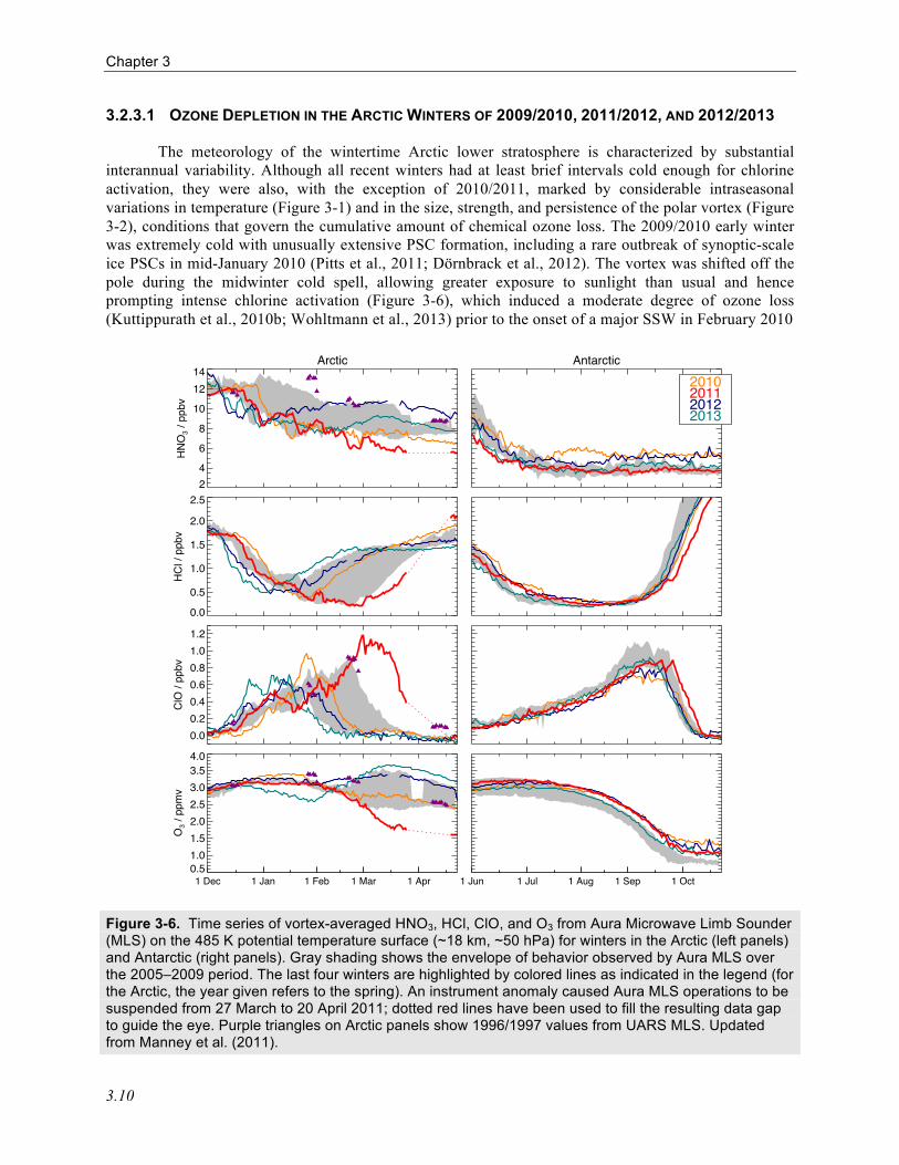
With the present availability of satellite stratospheric measurements, the extent of polar ozone destruction processes during the winter can be evaluated from the evolution of key species involved in those processes, such as hydrogen chloride (HCl), chlorine monoxide (ClO), and nitric acid (HNO3), in addition to ozone. Decreases in gas-phase HNO3 are indicative of the formation of PSCs, while decreases in HCl and increases in ClO signify the occurrence of chlorine activation through heterogeneous reactions on PSC particles and/or cold binary aerosols (see Section 3.3.1). Figure 3-6 (discussed in more detail below) shows the vortex-averaged evolution of these key constituents at a representative level in the lower stratosphere during the last four Arctic winters, as measured by the Microwave Limb Sounder (MLS) instrument onboard NASA’s Aura satellite. The envelope of behavior over the 2005–2009 period is also shown for comparison.

Chapter 3

 3.10

3.2.3.1 OZONE DEPLETION IN THE ARCTIC WINTERS OF 2009/2010, 2011/2012, AND 2012/2013

The meteorology of the wintertime Arctic lower stratosphere is characterized by substantial interannual variability. Although all recent winters had at least brief intervals cold enough for chlorine activation, they were also, with the exception of 2010/2011, marked by considerable intraseasonal variations in temperature (Figure 3-1) and in the size, strength, and persistence of the polar vortex (Figure 3-2), conditions that govern the cumulative amount of chemical ozone loss. The 2009/2010 early winter was extremely cold with unusually extensive PSC formation, including a rare outbreak of synoptic-scale ice PSCs in mid-January 2010 (Pitts et al., 2011; Dörnbrack et al., 2012). The vortex was shifted off the pole during the midwinter cold spell, allowing greater exposure to sunlight than usual and hence prompting intense chlorine activation (Figure 3-6), which induced a moderate degree of ozone loss (Kuttippurath et al., 2010b; Wohltmann et al., 2013) prior to the onset of a major SSW in February 2010

Figure 3-6. Time series of vortex-averaged HNO3, HCl, ClO, and O3 from Aura Microwave Limb Sounder (MLS) on the 485 K potential temperature surface (~18 km, ~50 hPa) for winters in the Arctic (left panels) and Antarctic (right panels). Gray shading shows the envelope of behavior observed by Aura MLS over the 2005–2009 period. The last four winters are highlighted by colored lines as indicated in the legend (for the Arctic, the year given refers to the spring). An instrument anomaly caused Aura MLS operations to be suspended from 27 March to 20 April 2011; dotted red lines have been used to fill the resulting data gap to guide the eye. Purple triangles on Arctic panels show 1996/1997 values from UARS MLS. Updated from Manney et al. (2011).

Arctic

24

6

8

10

1214

HN

O3 /

ppb

v

0.0

0.5

1.0

1.5

2.0

2.5

HC

l / p

pbv

0.00.20.40.60.81.01.2

ClO

/ pp

bv

0.51.01.52.02.53.03.54.0

O3 /

ppm

v

1 Dec 1 Jan 1 Feb 1 Mar 1 Apr

Antarctic

2010201120122013

1 Jun 1 Jul 1 Aug 1 Sep 1 Oct

Polar Ozone

 3.11

(Kuttippurath and Nikulin, 2012). Similarly, the 2011/2012 and 2012/2013 winters were characterized by low minimum temperatures in December that triggered PSC formation and chlorine activation. In late January 2012, a strong SSW (Chandran et al., 2013) halted further chemical processing. In December 2012 and January 2013, the vortex was again substantially shifted off the pole, ClO was strongly enhanced, and ozone abundances dropped (Figure 3-6). However, temperatures rose abruptly to near-record values in early January as a very strong and prolonged SSW began (Goncharenko et al., 2013). As a result, chlorine deactivation by early February 2013 precluded the exceptional loss that can occur when low temperatures persist into spring.

3.2.3.2 OZONE DEPLETION IN THE ARCTIC WINTER 2010/2011

The Arctic winter/spring of 2010/2011 has been widely studied. It was characterized by an unprecedented degree of chemical ozone loss, coupled with atypically weak transport of ozone to the lower stratospheric polar vortex, which led to exceptionally low values of springtime total ozone (Figures 3-4, 3-5, and 3-8). It must be emphasized, however, that the occurrence of this extreme event has not challenged our fundamental understanding of the processes controlling polar ozone. Unusual (for the Arctic) meteorological conditions in 2010/2011 resulted in record-low ozone through known chemical and dynamical mechanisms. If similar conditions were to arise again in the Arctic while stratospheric chlorine loading remains high, similarly severe chemical ozone loss would take place. Uncertainties in current climate models preclude confident quantification of the likelihood of repeated episodes of extensive Arctic ozone depletion in the present or future climate (e.g., Charlton-Perez et al., 2010; Garcia, 2011), as discussed in Section 3.5.

In spring 2011, the transport barrier at the edge of the lower stratospheric polar vortex was the strongest (in either hemisphere) in the previous 32 years (Manney et al., 2011). Unusually weak tropospheric planetary wave driving allowed the vortex to remain strong, stable, and cold for an extended period, with its mid-April breakup date one of the latest in the satellite era. The mechanisms responsible for the weak wave activity in 2011 have not been definitively determined but may be related to high sea surface temperatures in the North Pacific (Hurwitz et al., 2011; Section 3.3.3.2). Recent analyses suggest that the atypically high frequency of extreme total negative eddy heat flux events and the absence of extreme positive events at 50 hPa during spring 2011 may have contributed to weakened downward transport, cooling, and strengthening of the Arctic lower stratospheric vortex, and a delayed final warming (Shaw and Perlwitz, 2014). Daily minimum temperatures were only moderately low (i.e., rarely below ice PSC formation thresholds), but the cold region was uncommonly long lasting and vertically extensive, leading to a winter-mean vortex fractional volume of air with the potential for PSC formation that was the largest ever observed in the Arctic (Manney et al., 2011), and a March Arctic polar cap temperature at 50 hPa more than two standard deviations below the climatological mean (Hurwitz et al., 2011). The persistence of a strong, cold vortex for more than three months (from December through the end of March) is typical in the Antarctic but unique in the observational record in the Arctic (Manney et al., 2011).

Consistent with the temperature distribution, ice PSCs were rare, but other PSCs types (see Box 3-1, p. 3.17) were abundant until mid-March (Arnone et al., 2012; Lindenmaier et al., 2012). CALIPSO data show that not only were PSCs present far later in 2011 than is typical in the Arctic, but they also spanned a vertical range comparable to that in the Antarctic (Manney et al., 2011). Widespread and persistent PSCs led to severely depleted gas-phase HNO3 (Figure 3-6). That HNO3 mixing ratios remained much lower than observed in any previous Arctic winter well after the last PSCs had dissipated is evidence for the occurrence of considerable denitrification (Sinnhuber et al., 2011; Kuttippurath et al., 2012).

The persistent low temperatures supported extensive chlorine activation on the surfaces of PSC particles and/or cold binary aerosols. Although some chlorine activation has occurred in all recent Arctic winters, it has never been as prolonged or as intense as that in 2011, when vortex-averaged ClO values exceeded the range previously observed in the Arctic from late February through March (Manney et al.,

Chapter 3

 3.12

2011). In addition, very low values of chlorine nitrate (ClONO2) (Sinnhuber et al., 2011; Arnone et al., 2012; Lindenmaier et al., 2012) and HCl (Figure 3-6) were observed in the vortex in March. In contrast to previous cold Arctic winters, when chlorine deactivation had already been completed by mid-March, in 2011 ClO began decreasing rapidly only about a week earlier than is typical in the corresponding season in the Antarctic (Figure 3-6). For the ozone and odd nitrogen abundances normally found in the Arctic, the primary chlorine deactivation mechanism is the reformation of ClONO2, whereas under the severely denitrified and ozone-depleted conditions characteristic of the Antarctic ozone hole, production of ClONO2 is suppressed and that of HCl favored. Figure 3-6 shows that chlorine was initially repartitioned into HCl to a greater (more Antarctic-like) extent than typical in the Arctic, suggesting that denitrification and low ozone abundances may have inhibited ClONO2 reformation to some extent (Manney et al., 2011; Arnone et al., 2012; Lindenmaier et al., 2012). Nevertheless, the steep rise in ClONO2 associated with the decline in ClO after mid-March indicates that deactivation did occur predominantly into that reservoir even in 2011 (Sinnhuber et al., 2011; Arnone et al., 2012).

The meteorological conditions (persistent low temperatures inside a strong, isolated polar vortex), consequent chlorine activation, and denitrification in the 2011 Arctic vortex led to severe chemical ozone destruction between 16 and 22 km altitude (Figure 3-7), with 60–80% of the vortex ozone at ~18–20 km removed by early April (Manney et al., 2011; Sinnhuber et al., 2011). Because of the delayed chlorine deactivation, lower stratospheric ozone loss rates in March 2011 reached over 4 parts per billion by volume (ppbv) per sunlit hour (Kuttippurath et al., 2012) or 0.7%/d (Pommereau et al., 2013), larger than previously observed in mid-March in the Arctic and similar to those routinely seen in September in the Antarctic. Peak chemical ozone loss had been as large in some previous cold Arctic winters (e.g., the winters of 2000 and 2005; Manney et al., 2011), but significant loss extended over a much broader altitude region in 2011 (Manney et al., 2011). In addition to chemical ozone destruction, unusually weak diabatic descent and wave-driven horizontal transport also played major roles in 2011, with the late final warming delaying influx of ozone-rich air into the polar lower stratosphere (Hurwitz et al., 2011; Isaksen et al., 2012; Strahan et al., 2013). Although CTM studies consistently show that the exceptionally low

Figure 3-7. Profiles of observed vortex-average chemical ozone loss from the cold Arctic winter/spring periods of 1997 and 2011 derived from ozonesondes. Note that significant differences (up to ~0.4 parts per million by volume (ppmv) at the end of March 2011) in ozone loss estimates for a given year derived from various methods and data sets imply some uncertainty in the chemical loss determination. However, year-to-year differences in the amount of ozone loss obtained from any given method/data set combination are very similar, indicating a high degree of precision in the relative amount of calculated loss between different years and hemispheres. Also shown is an indicative range of ozone loss for typical Antarctic winter/spring periods, illustrated by the loss that has been derived from ozone observations for a relatively weak early Antarctic ozone hole (1985, upper limit of the gray shading) and the loss in a strong Antarctic ozone hole (2003, lower limit of the gray shading). Error bars show uncertainty estimates of the derived ozone losses based on a methodology described in Harris et al. (2002). Figure adapted from Manney et al. (2011).

Polar Ozone

 3.13

ozone abundances in spring 2011 were brought about by both extreme chemical loss and weak dynamical resupply, they disagree on the relative contributions of the two factors, with Isaksen et al. (2012) attributing roughly 25% of the observed ozone column anomaly to chemistry and the rest to transport effects, whereas Strahan et al. (2013) found chemical and transport effects to contribute equally.

Together, the anomalous chemical and meteorological conditions induced record-low ozone in March 2011, as characterized by a variety of metrics. Sinnhuber et al. (2011) reported Michelson Interferometer for Passive Atmospheric Sounding (MIPAS) measurements showing that vortex-averaged ozone at 475 K decreased from ~3 parts per million by volume (ppmv) in early December to ~1.5 ppmv in early April, in good agreement with the MLS measurements shown at 485 K in Figure 3-6. Using Ozone Monitoring Instrument (OMI) data, Manney et al. (2011) calculated that the fraction of the Arctic vortex in March with total ozone less than 275 Dobson units (DU), typically near zero, reached nearly 45% in 2011 (see also Figure 3-8); minimum vortex total ozone values were continuously below 250 DU for 27 days. Integrated over the column, the 2011 Arctic ozone “deficit” (the difference between the daily total ozone amount from OMI and a reference value minimally affected by chemical ozone loss) was comparable to that in the Antarctic vortex core in recent years (Figure 3-8; Manney et al., 2011). Similarly, column ozone measurements from UV-visible spectrometers located in eight Systèmes d’Analyse par Observation Zénithale (SAOZ)/NDACC stations distributed around the Arctic indicate a reduction in total ozone of ~38% (170 DU) by late March 2011, the largest in the SAOZ record dating back to 1994 and comparable to that in the 2002 Antarctic winter (Pommereau et al., 2013). Ground-based measurements at the Polar Environment Atmospheric Research Laboratory (PEARL) at Eureka, Canada, also registered the lowest ozone columns in their 11-year record, 237–247 DU, when the vortex was overhead in mid-March (Adams et al., 2012). On the basis of the long-term total ozone data set updated from Stolarski and Frith (2006), in 2011 March total ozone averaged over the 60–80°N region was the lowest of the satellite era (Hurwitz et al., 2011; see also Figure 3-4). Similarly, record-low zonal mean (60–90°N) column ozone values, reaching as low as ~310 DU in mid-March, were seen in Global Ozone Monitoring Experiment 2 (GOME-2) data (Balis et al., 2011; Isaksen et al., 2012).

It is important to emphasize that because downward transport in the winter polar vortex is stronger in the Arctic, background ozone levels are ~100 DU higher there than in the Antarctic (e.g., Tegtmeier et al., 2008). As a result, although the evolution of Arctic ozone and related constituents in spring 2011 more closely followed that characteristic of the Antarctic than ever before, the springtime total ozone values remained considerably higher than those reached in a typical year in the Antarctic (Figures 3-4, 3-5, and 3-8). Moreover, ozone loss in cold and prolonged Antarctic winters is substantially greater throughout the profile (Figure 3-7). Finally, because the areal extent of the 2011 Arctic vortex was only ~60% the size of a typical Antarctic vortex, the low-ozone region was more spatially confined (Figure 3-8).

Figure 3-8. Maps of total column ozone from Aura Ozone Monitoring Instrument (OMI) (top row) and ozone “deficit” (bottom row) for the Arctic (left) and Antarctic (right). Total ozone deficit is defined as the difference between daily values and a reference total ozone field minimally affected by chemical loss. Overlaid black contours mark the size and shape of the polar vortex on the 460 K potential temperature surface. Adapted from Manney et al. (2011).  

 

26 Mar 2011 26 Sep 2010

280 320 360 400 440

Col

umn

O3 (

DU

)

26 Mar 2011 26 Sep 2010

-110 -70 -30 10 50

Col

umn

Def

icit

(DU

)

Chapter 3

 3.14

3.2.3.3 TWO ARCTIC SPRINGS WITH VERY LOW TOTAL OZONE: 1997 AND 2011

Figure 3-4 shows that March polar-cap average total ozone abundances were comparably low in 1997 and 2011, and much lower than those in any other year in the satellite record. Similarly, Figure 3-5 shows that the minimum daily mean ozone column amount reached in March was very low in both 1997 and 2011, although in this view 2000 was also an exceptional year, and the 1997 value is not as striking. As discussed in Section 3.2.3.2, an unprecedented degree of chemical ozone loss took place in 2011, whereas only moderate chemical ozone loss occurred in 1997 (Manney et al., 1997; Tegtmeier et al., 2008). In fact, chemical loss also was more severe in the Arctic springs of 1996 and 2005 than in 1997 (WMO, 2007; Manney et al., 2011; Pommereau et al., 2013), yet those years show larger March average total ozone in both Figures 3-4 and 3-5. That the March total ozone values in these two years are so similar reflects how strongly Arctic column ozone is influenced by dynamical effects (e.g., Petzoldt, 1999; Tegtmeier et al., 2008). Here, the chemical and dynamical conditions in the two years are compared and contrasted to underline the fact that total ozone abundances cannot by themselves be used as a proxy for quantifying chemical loss in the lower stratosphere. Similarities between 1997 and 2011: • The polar stratospheric chlorine burden peaked in the period 2000–2002 and has been declining

slowly since then (WMO, 2011; see also Chapter 1); thus the amount of total inorganic chlorine available was approximately the same in the two years.

• Lower stratospheric temperatures below the threshold associated with chlorine activation on PSC particles and/or cold binary aerosols (see Section 3.3.1) persisted through March in both years (Coy et al., 1997; Manney et al., 2011; Figure 3-1), prolonging the potential for heterogeneous processing into a period of greater exposure to sunlight than in more typical years.

• The lower stratospheric vortices were unusually persistent into the spring, consistent with abnormal patterns of total eddy heat fluxes at 50 hPa (Shaw and Perlwitz, 2014); as a result, vortex breakup dates in both years were among the latest on record, delaying dynamical resupply of ozone to northern high latitudes and keeping March total ozone abundances anomalously low (Hurwitz et al., 2011; Isaksen et al., 2012; Strahan et al., 2013).

Differences between 1997 and 2011: • The transport barrier at the edge of the 2011 Arctic vortex was unusually strong throughout the winter

(the strongest on record during February and March), whereas the 1997 vortex was among the weakest until February, and near average strength thereafter (Manney et al., 2011).

• Lower stratospheric minimum temperatures were continuously below the threshold for chlorine activation (through heterogeneous reactions on PSC particles and/or cold binary aerosol; see Section 3.3.1) from mid-December through March in 2011 (Manney et al., 2011), whereas they did not drop significantly below that threshold until mid-January in 1997 (Coy et al., 1997; Figure 3-1)

• Temperatures persistently (for more than 100 days) below the chlorine activation threshold covered a larger vertical domain in 2011 than in 1997 (15–23 km vs. 20–23 km), with a consequently broader range of ClO enhancement as well as larger maximum ClO abundances, especially at lower altitudes (Manney et al., 2011).

• Early-winter cold conditions and chlorine activation prompted ozone destruction, resulting in ~0.7–0.8 ppmv less O3 at lower stratospheric levels by March in 2011 than in 1997 (Figure 3-6).

• The persistent cold in 2011 led to extensive PSC formation and severe denitrification (Sinnhuber et al., 2011; Arnone et al., 2012; Lindenmaier et al., 2012), with ~4 ppbv less HNO3 at lower stratospheric levels by March in 2011 than in 1997 (Figure 3-6).

• Denitrification delayed chlorine deactivation in 2011, when ClO started to decline rapidly only in mid-March (Figure 3-6), compared to late February in 1997 (Santee et al., 1997); the late onset of chlorine deactivation allowed ozone loss rates in March 2011 to reach values typical in the Antarctic

Polar Ozone

 3.15

at an equivalent time but not observed previously in the Arctic at this period of time (Kuttippurath et al., 2012; Pommereau et al., 2013).

• Photochemical box model results suggest that by prolonging the period of rapid springtime ozone destruction, denitrification caused an additional 0.6 ppmv of loss in March and April 2011 (Manney et al., 2011).

• Together, the early-winter loss and greater springtime loss induced by denitrification roughly account for the ~1.5 ppmv lower ozone observed in the lower stratosphere in 2011 than in 1997 (Manney et al., 2011).

In summary, anomalous meteorological conditions played a large role in bringing about low total

ozone in the Arctic springs of both 1997 and 2011. Chlorine-catalyzed ozone destruction was much greater in 2011 than in 1997. Although a cold polar vortex persisted into April in both years, chemical loss as severe as that in 2011 requires additional conditions that did not occur in 1997, namely: temperatures low enough to trigger chlorine activation early in winter, and cold regions extensive enough to allow widespread denitrification before March. Even in 2011, however, denitrification was not so severe and vertically extensive as to allow ozone destruction on the scale typically seen in Antarctica over a large altitude range (e.g., Manney et al., 2011; Arnone et al., 2012; Solomon et al., 2014).

3.2.4 Recent Antarctic Winters

The Antarctic winters of 2010, 2012, and 2013 were on average characterized by larger ozone columns than has been typical for the Antarctic stratosphere since the early 1990s (Figure 3-4). The ozone mass deficits (OMD) during those years were approximately one-third smaller than during most years of the 2000s, and losses were close to half of the maximum recorded OMD in 2006 (based on the Multi Sensor Reanalysis (MSR) total ozone data set, following de Laat and van Weele, 2011). In contrast, in 2011 the reduction of springtime Antarctic ozone columns was more typical of that observed in the 2000s.

The 2010 Antarctic vortex was characterized by a midwinter (mid-July) minor SSW, which increased the descending motion within the polar vortex (a minor SSW is a warming not accompanied by a 10 hPa zonal wind reversal around 65ºS). Correspondingly, VPSC, the potential NAT volume (see Section 3.2.2.3) based on MERRA reanalysis data remained well below the 1979–2012 average and less denitrification than typical occurred during the Antarctic winter of 2010. The SSW penetrated down to 50 hPa. The average temperature between 60º-90ºS around 30 hPa rose by approximately 5–10 K from 190 K to 195–200 K and thus above the threshold temperature for efficient heterogeneous chlorine activation. As a result, in 2010 photochemical springtime ozone destruction around 30 hPa became less effective. Combined with a late onset of ozone depletion around 30 hPa within the vortex which occurred two to four weeks later than typical during the last decade (de Laat and van Weele, 2011; Klekociuk et al., 2011) ozone columns throughout the 2010 Antarctic spring remained larger than what has been typical for the 2000s. Note that, as midlatitude wave activity remained weak during the rest of the winter and spring, the vortex remained stable into December.

The occurrence of an Antarctic ozone hole with much less ozone loss is not without precedent. Other years that have shown less than typical (for the period) Antarctic ozone loss are 1986, 1988, 2002, and 2004. It has long been established that the much lower ozone loss during these years compared to previous years is related to above-average wave activity (e.g., Schoeberl et al., 1989; Kanzawa and Kawaguchi, 1990; WMO, 2007). Furthermore, it is well documented that this reduction occurred at altitudes between approximately 20 and 25 km (Hofmann et al., 1997; Hoppel et al., 2005), above the 15–20 km layer typically associated with complete ozone destruction.

Using trace gas measurements from Aura MLS, de Laat and van Weele (2011) showed that the primary cause of the smaller ozone loss in 2004 and 2010 was a change in chemistry triggered by vortex dynamics. Enhanced midlatitude wave activity induced SSWs during the Antarctic winter (July–August). Although the amplitude of these minor warmings is small in an absolute sense—only a few degrees

Chapter 3

 3.16

Kelvin at maximum and not comparable to the magnitude of sudden warmings seen in the Arctic—they nevertheless strongly inhibit the formation of PSCs at altitudes between 20 and 25 km where temperatures are close to PSC formation thresholds. The reduced PSC formation limits denitrification and dehydration as seen in water vapor and nitric acid measurements from MLS. Due to this pre-conditioning, once sunlight returns to the Antarctic stratosphere from mid-August onward, reduced availability of active halogen lessens the efficiency of catalytic ozone destruction.

In 2011, stratospheric temperatures during Austral winter and spring remained persistently lower than the long-term mean and on average close to the lowest stratospheric temperatures seen since 1979 throughout, with only a single small warming period during midwinter. Estimates of the potential NAT volume in 2011 were well above its climatological mean, and ozone destruction was not reduced.

In 2012, meteorological conditions to some extent mimicked those in 2010, i.e., in early winter (late June) a minor SSW occurred, which reduced the potential NAT volume and preconditioned the Antarctic lower stratosphere for less ozone depletion. However, the 2012 winter SSW was not as pronounced as that in 2010. On the other hand, in contrast to 2010, springtime 2012 was characterized by several minor SSWs. As a result, stratospheric temperatures between 10 to 50 hPa remained above the long-term climatological mean. These minor warmings were indicative of a less stable vortex, which led to an early dissipation of the Antarctic vortex halfway through October (Kramarova et al., 2014). This explains the relatively large total ozone column values in October 2012 in Figures 3-4 and 3-5.

In 2013, no midwinter warming events occurred. Yet, from mid-August onward, the Antarctic vortex was disrupted by several minor SSWs, mimicking the year 2012 with stratospheric temperatures between 10 to 50 hPa remaining above the long-term climatological mean, and similar to 2013, an early dissipation of the vortex.

Note that detailed analyses of the 2012 and 2013 Antarctic ozone hole seasons have not been performed at the time of this Assessment. Hence, it is not known to what degree modified chemistry and changes in vortex dynamics and transport processes have contributed to the smaller than typical OMDs in 2012 and 2013.

In summary, the Antarctic ozone hole has seen very different amounts of ozone loss over the period 2010–2013 due to variations in polar vortex dynamics. In particular, minor SSWs, as well as reduced vortex stability, have led to significantly reduced Antarctic springtime ozone depletion during several years.

3.3 UNDERSTANDING OF POLAR OZONE PROCESSES

Overall, there have been no major changes in our understanding of polar ozone loss processes since WMO (2011). Our knowledge of polar chemical and dynamical processes was already based on a large body of research, and models could reproduce observed chemical polar ozone depletion and its variability well (e.g., Chipperfield et al., 2005; Frieler et al., 2006). Recent work has improved our detailed understanding of polar ozone processes, such as the formation mechanism of nitric acid trihydrate (NAT) particles; validated previous assumptions; and reduced uncertainty. For example, uncertainty in the photolysis rate of the ClO dimer (Cl2O2 or ClOOCl), a key parameter in polar chemical ozone loss, has been reduced by a factor of three (see Section 3.3.2.2). The very cold winter of 2010/11 increased the range of meteorological variability seen in the Arctic over the past few decades and provided a new extreme test case for models.

3.3.1 Polar Stratospheric Clouds

Polar stratospheric clouds (PSCs) play two major roles in stratospheric ozone depletion (Solomon, 1999). First, heterogeneous chemical reactions that convert chlorine from HCl and ClONO2 reservoirs to active, ozone-destroying species are catalyzed by PSC particles (primarily supercooled ternary solution (STS) droplets; see Box 3-1), as well as by cold binary aerosols (Portmann et al., 1996;

Polar Ozone

 3.17

Drdla and Müller, 2012). Second, the gravitational sedimentation of large nitric acid trihydrate (NAT) PSC particles irreversibly removes gaseous odd nitrogen (denitrification) (Salawitch et al., 1989), thereby slowing the reformation of the benign chlorine reservoirs and extending the ozone depletion process.

3.3.1.1 RECENT OBSERVATIONS

An extensive set of PSC observations was produced by the RECONCILE field campaign conducted in the Arctic during January–March 2010 (von Hobe et al., 2013). These include observations from in-situ particle probes, a HNO3 content probe, in situ backscatter probe, infrared limb-sounding instrumentation, and upward- and downward-looking lidar onboard the high-altitude M55-Geophysica aircraft; from ground-based lidars; and from the balloon-borne Compact Optical Backscatter and AerosoL Detector (COBALD) aerosol backscatter sondes. In addition, the spaceborne lidar (Cloud-Aerosol Lidar with Orthogonal Polarization, CALIOP) on the Cloud-Aerosol Lidar and Infrared Pathfinder Satellite Observation (CALIPSO) satellite provided a view of PSC properties on nearly vortex-wide spatial scales and spanning the entire winter, complementing the more localized campaign measurements. Significant findings related to PSC processes include:  

1) Extensive regions of NAT PSCs were observed by CALIOP during 15–30 December 2009 prior to the occurrence of ice PSCs (Pitts et al., 2011). This is the first time NAT PSCs have been observed on vortex-wide scales prior to the occurrence of ice PSCs and corroborates the conclusions of Pagan et al. (2004) and Voigt et al. (2005) that ice nuclei are not a prerequisite for NAT formation. A non-ice NAT nucleation mechanism operating on vortex-wide scales has important implications for denitrification and potential enhancement of ozone depletion.

Box 3-1. Stratospheric Particles and Their Roles in Ozone Depletion

• Stratospheric aerosols – liquid sulfuric acid/water (H2SO4/H2O) droplets: They are present at all latitudes in the lower stratosphere; typical mean radius ≈ 0.05–0.1 µm. Their background abundance can be greatly enhanced by volcanic eruptions that reach the stratosphere. These aerosols cause the conversion of gaseous nitrogen oxides (NOx: NO + NO2) species to nitric acid (HNO3) and can initiate chlorine activation at low temperatures (≈ 195 K).

• Supercooled ternary solution (STS) polar stratospheric clouds (PSCs) – liquid nitric acid/sulfuric acid/water (HNO3/H2SO4/H2O) droplets: They grow from stratospheric aerosols at low temperatures (≈195 K) without a phase change; maximum radius ≈0.3–0.5 µm. They are responsible for reversible removal of HNO3 by condensation and play a major role in chlorine activation.

• Solid nitric acid trihydrate (NAT) PSCs – HNO3•3 H2O particles: They can form at temperatures below the NAT existence temperature, typically around 195 K, but require significant super-cooling to form readily from the gas or liquid phase. They are responsible for irreversible removal of HNO3 (denitrification) when they sediment and can play a role in chlorine activation, though their effect is likely masked by activation on STS particles. NAT particles have a typical radius of 1 µm, but can grow to 10 µm radius or larger. These larger particles have been referred to as “NAT-rocks.”

• Solid water ice PSCs – H2O particles: They can exist only at temperatures below the frost point, typically around 188 K; typical radii range from ~1 µm for mountain wave-induced ice PSCs to 5–10 µm for synoptic-scale ice PSCs. They are responsible for irreversible removal of H2O (dehydration) but play a minor role in chlorine activation.

Chapter 3

 3.18

2) Unusually large PSC particles (“NAT-rocks”) were detected during the 2010 winter and again in the winter of 2011 when synoptic scale PSCs formed in the Arctic (von Hobe et al., 2013). Visual evidence for particles with diameters as large as 35 µm was provided by shadow-cast images. However, if the particles are assumed to be NAT spheres, the total mass of all optically detected particles with diameters greater than 2 µm exceeds the available total reactive nitrogen (NOy) (as measured and also reconstructed from model calculations) beyond the measurement uncertainties. Thus, new theoretical concepts, e.g., that the particles are highly aspherical or consist mostly of ice with a NAT coating, must be explored.

3) In situ measurements of submicron background aerosols showed that up to 75% of the particles larger than 10 nm in diameter were non-volatile or contained non-volatile cores and thus could not consist solely of sulfuric acid (H2SO4) and H2O (von Hobe et al., 2013). This high refractory particle fraction was consistently found within the Arctic polar vortex during three measurement campaigns in 2003, 2010, and 2011, with the largest amount of refractory material occurring at the lowest nitrous oxide (N2O) mixing ratios. Thus, subsiding air masses in the vortices transported non-volatile particulate matter—possibly of meteoric origin—from the upper stratosphere and lower mesosphere into the upper troposphere/lower stratosphere (UT/LS) region. Especially in times of relative volcanic quiescence or low stratospheric background (H2SO4/H2O) aerosol, such particles may be involved in heterogeneous PSC nucleation (e.g., Hoyle et al., 2013; Engel et al., 2013).

4) A rare outbreak of synoptic-scale Arctic ice PSCs was observed by CALIOP from 15–21 January 2010. During this same period, unprecedented evidence of water redistribution and irreversible dehydration in the Arctic stratosphere was obtained (Engel et al., 2014). Simultaneous balloon-borne measurements of water vapor and aerosol backscatter on 17 January provided a unique high-resolution snapshot of repartitioning of water vapor into ice particles. For the first time, signatures of rehydration could be measured in the Arctic and attributed to the observed dehydration. The movement of the dehydrated air masses around the polar vortex was seen in the Aura MLS water vapor data. A modeling study by Engel et al. (2014) showed that the observed redistribution of water cannot be explained by homogeneous ice nucleation alone. A selective, heterogeneous nucleation mechanism is required that allows the ice particles to grow to larger sizes compared to homogeneously nucleated ice particles, which remain too small to cause the significant dehydration in the observed case.

3.3.1.2 REVISED HETEROGENEOUS NAT AND ICE NUCLEATION SCHEME

The formation of NAT PSCs is a prerequisite for denitrification by sedimenting particles, which prolongs seasonal ozone loss. The extensive and deep denitrification in the Antarctic vortex helps to drive the almost complete O3 loss inside the Southern Hemisphere polar vortex (Solomon et al., 2014). In contrast, denitrification in the Arctic is smaller and more variable from year to year. A more accurate representation of NAT PSC nucleation and particle characteristics leads to better model simulations of denitrification and hence ozone loss. For example, a Single-Layer Isentropic Model of Chemisty and Transport (SLIMCAT) chemical transport model (CTM) simulation of the 2004/2005 Arctic winter using the microphysics-based Denitrification by Lagrangian Particle Sedimentation (DLAPSE) denitrification scheme showed much better agreement with observed HNO3 and column O3 loss than a simulation using the standard thermodynamic equilibrium PSC approach (Feng et al., 2011).

CALIOP observations of widespread NAT PSCs and synoptic-scale ice PSCs in the Arctic during the 2009/2010 winter (Pitts et al., 2011) have stimulated new microphysical modeling studies (Hoyle et al., 2013; Engel et al., 2013). PSC optical parameters computed using Mie and T-Matrix scattering codes were compared to selected CALIPSO PSC observations made in December 2009 and January 2010. The best agreement between model and observations was achieved by (1) allowing for NAT and ice to

Polar Ozone

 3.19

nucleate heterogeneously on pre-existing solid particles and (2) superimposing small-scale temperature fluctuations onto synoptic-scale parcel trajectories as suggested by Murphy and Gary (1995). The nucleation properties of NAT and ice can be approximated the same way as heterogeneous ice nucleation on Arizona test dust in the immersion mode as demonstrated in previous laboratory experiments (Marcolli et al., 2007). Whereas artificially produced Arizona test dust is composed of various mineral species with a composition similar to that of dust originating from desert, non-volatile solid inclusions were observed in 67% of the stratospheric background aerosols by Curtius et al. (2005) and up to 75% of the submicron aerosol measurements during the 2010 RECONCILE campaign (von Hobe et al., 2013). Coagulated meteoritic smoke particles or micrometeorites may be suitable nuclei for heterogeneous NAT and ice formation as speculated by the above mentioned authors and have also been used in early laboratory experiments by Biermann et al. (1996). It now appears that the upper limits of measured NAT nucleation rate coefficients on foreign material by Biermann et al. (1996) might be sufficient to explain the CALIPSO PSC observations of low number density NAT PSCs from December 2009.

The newly introduced heterogeneous nucleation pathways of NAT and ice are allowed to compete with the conventional accepted pathways of PSC formation, namely, the growth of liquid particles into supercooled ternary solution (STS) droplets due to uptake of HNO3 and H2O (Carslaw et al., 1995), the homogeneous ice nucleation at around 3 K below the ice frost point (Koop et al., 2000), and the subsequent nucleation of NAT on ice upon warming, which typically occurs in mountain-wave-driven localized cold pools (Carslaw et al., 1998).

Grooß et al. (2014) implemented a new saturation-dependent NAT nucleation parameterization into the Chemical Lagrangian Model of the Stratosphere (CLaMS) model based on the theory described in Hoyle et al. (2013) and found that the model reproduces the locations and extent of NAT PSCs observed by CALIOP somewhat better than when a constant nucleation rate is assumed (Grooß et al., 2005).

3.3.1.3 IMPROVED UNDERSTANDING OF PSC COMPOSITION

Recent studies by Lambert et al. (2012) and Pitts et al. (2013) demonstrated the usefulness of combining nearly coincident data from the CALIOP lidar on CALIPSO and MLS on Aura to study the temperature-dependent uptake of HNO3 in PSCs; this procedure is very similar to the method of Spang and Remedios (2003), who combined Cryogenic Infrared Spectrometers and Telescopes for the Atmosphere (CRISTA) measurements of HNO3 and particle properties for a PSC type classification in the Southern Hemisphere. Comparing observations with theoretical HNO3 uptake for STS (Carslaw et al., 1995) and NAT (Hanson and Mauersberger, 1988) allows one to judge how well PSCs can be assigned to the various composition classes by CALIOP and also offers insight into PSC growth kinetics. Pitts et al. (2013) showed that CALIOP PSCs in the STS, liquid-NAT mixture (external mixtures of NAT and stratospheric aerosols or STS), and ice classes conform well to their expected temperature existence regimes, providing more confidence in our understanding of PSC particle composition. Pitts et al. (2013) also found that liquid-NAT mixture PSCs exhibit two preferred modes of HNO3 uptake, one that is closely aligned with the theoretical HNO3 uptake curve for STS, and a second that is more closely aligned with the theoretical HNO3 uptake curve for NAT as shown in Figure 3-9a.

Analysis of temperature histories along parcel trajectories (Figure 3-9b) show that liquid-NAT mixture PSCs with HNO3 uptake more like that of STS had been below the NAT existence temperature TNAT for only short periods of time. Since the growth of large, low-number-density NAT particles is kinetically limited, HNO3 uptake in these mixtures of PSCs is dominated by STS droplets. On the other hand, liquid-NAT mixture PSCs with HNO3 uptake more like that of NAT had been below TNAT for much longer periods of time, allowing the thermodynamically favored NAT particles to approach equilibrium (Figure 3-9b). Wegner et al. (2013) showed that allowing the formation of non-equilibrium NAT mixtures in the Whole Atmosphere Community Climate Model (WACCM) global 3-D model significantly improves the agreement of the model with gas-phase HNO3 observations.

Chapter 3

 3.20

Figure 3-9. (a) Uptake of nitric acid as a function of T − Tice for CALIOP Arctic NAT mixture PSC observations during 1 December 2009–31 January 2010. (b) Temperature histories along air parcel trajectories for CALIOP Arctic NAT mixture PSC observations during 1 December 2009–31 January 2010. The color scale for panel (b) indicates the average number of hours each air parcel associated with the NAT mixture observations falling within each bin was exposed to temperatures below TNAT. Black lines are reference equilibrium uptake curves for STS and NAT assuming 16 ppbv HNO3 and 5 ppbv H2O. The histogram bin size is 0.25 ppbv × 0.25 K. Adapted from Pitts et al. (2013).

3.3.1.4 PSC FORCING MECHANISMS

PSCs can form in the winter polar stratosphere once the synoptic-scale temperature drops below the NAT and ice PSC existence temperatures, but the formation of NAT particles requires significant supercooling below the NAT equilibrium temperature. Small-scale orographic gravity waves provide an additional forcing mechanism for PSC formation when synoptic-scale temperatures are close to the PSC formation thresholds (Godin et al., 1994; Carslaw et al., 1999). The PSCs formed by orographic gravity waves can cause the conversion of a large fraction of inactive chlorine species to reactive chlorine species (Carslaw et al., 1998), despite the limited spatial and temporal scales of the waves. Early-season PSC formation in the Antarctic winter has been linked to orographic wave forcing (Höpfner et al., 2006; Eckermann et al., 2009), with quantifiable changes in the abundance of trace gas species (Lambert et al., 2012). PSC formation due to orographic wave forcing occurs throughout winter near the polar vortex edge, where synoptic-scale temperatures remain close to the frost-point temperature (Alexander et al., 2011; Kohma and Sato, 2011). Recent satellite data sets indicate the occurrence of midwinter PSCs linked to orographic wave forcing in both the Arctic and the Antarctic (Khosrawi et al., 2011; Noel and Pitts, 2012; Alexander et al., 2013). Analyses of satellite observations indicate that the location and occurrence of resolved orographic gravity waves are well reproduced by meteorological analyses such as ECMWF, but the amplitudes can be significantly underestimated (e.g., Schroeder et al., 2009). Kohma and Sato (2013) demonstrated that the simultaneous occurrence of upper tropospheric clouds and PSCs is preferentially promoted by tropospheric blocking linked to high-pressure systems.

Polar Ozone

 3.21

3.3.2 Polar Chemistry

3.3.2.1 HETEROGENEOUS CHEMISTRY

During polar winter, heterogeneous reactions can convert reservoir chlorine species (HCl and ClONO2) into more reactive species, together termed ClOx, that destroy ozone (Solomon et al., 1986). The seasonal evolution of the balance between the heterogeneous chlorine activation rates and mostly gas-phase chlorine deactivation rates (i.e., the reformation of HCl and/or ClONO2) largely controls the amount of ozone loss in a given polar winter.

Chlorine activation reactions occur on a variety of surface types such as liquid binary aerosol, STS, and NAT (Box 3-1), although with rates that, at a given temperature, vary with the surface type and increase substantially with decreasing temperature. All of these particles are included in typical models used to simulate stratospheric ozone. Drdla and Müller (2012) proposed that the temperature threshold for the onset of polar chlorine activation is controlled by the reactivity of liquid aerosols. They further report that different assumptions about the types of PSC and rates of heterogeneous reactions have only a minor impact on simulated polar chlorine activation rates, at least for the range of conditions studied (the Arctic winter 1999/2000 and the Antarctic winter 2000). Fast chlorine activation on liquid particles means that these particles control the onset of polar chlorine activation at temperatures just higher than TNAT, and Drdla and Müller (2012) argue they are sufficient to reproduce the morphology of chlorine activation and the evolution of ClOx levels throughout winter. They suggest that this is the case even for cold binary (H2SO4/H2O) stratospheric aerosols. In reality, these particles will take up HNO3 as temperatures decrease, turning them into STS and further increasing their reactivity. Wohltmann et al. (2013) found that the difference in simulated column ozone loss over the winter 2009/2010 caused by a variety of assumptions about heterogeneous activation rates is less than 10%. For other winters it remains to be studied how sensitive ozone loss calculations are to these assumptions. When temperatures remain low until later during the season compared to 2009/2010, these sensitivities can potentially be larger.

Vortex-averaged satellite observations by the MLS instrument for the Arctic winters 2004/2005 to 2010/2011 (Figure 3-10) show that the initial removal of HCl and HNO3 from the gas-phase in December/January are not correlated (Wegner et al., 2012) and therefore there is no definite connection between the PSC particles that lead to chlorine activation and those that deplete gas-phase HNO3. HNO3 loss exhibits large interannual variability depending on prevailing temperatures while HCl loss is continuous through December with small inter- or intra-annual variability. Hence, the occurrence of HNO3-containing PSC particles does not seem to have a significant effect on the rate of initial chlorine activation on a vortex-wide scale.

Figure 3-10. HCl and HNO3 observations by MLS for the Arctic winters 2004/2005 to 2010/2011 on 500 K potential temperature in the vortex core (equivalent latitude >75°N). Adapted from Wegner et al. (2012).

Chapter 3

 3.22

Overall the body of work presented above corrobates the view that chlorine activation rates are mainly controlled by temperature (e.g., Kawa et al., 1997), with a limited dependence on the different particle types. Nonetheless, the formation of STS and NAT particles is important as these particles significantly alter gas-phase chemistry through the uptake of HNO3. Further, the formation of NAT particles is important as sedimentation and thus denitrification can only occur if large NAT particles form in the stratosphere (see Section 3.3.1).

Antarctic observations have shown that extremely low ozone mixing ratios below about 0.5 ppmv are reached (e.g., Solomon, 2005). The lower limit of these low ozone values has been investigated by Grooß et al. (2011), extending earlier work by Douglass et al. (1995). Grooß et al. showed that continuous rapid heterogeneous reactions on polar stratospheric clouds were required to produce the extreme low ozone values observed in the Antarctic. They show that under such low ozone conditions with continued PSC existence a balance is maintained by gas-phase production of both HCl and hypochlorous acid (HOCl) followed by heterogeneous reaction between these two compounds, which inhibits deactivation of chlorine via the formation of HCl and therefore allows the ozone loss to continue. Thereafter, a very rapid, irreversible chlorine deactivation into HCl occurs, either when ozone drops to values low enough for gas-phase HCl production to exceed chlorine activation processes or when temperatures increase above the polar stratospheric cloud formation threshold.

3.3.2.2 GAS-PHASE CHEMISTRY

Recent observational studies and laboratory investigations have largely confirmed our understanding of how chlorine and bromine compounds drive polar ozone losses. The major cause of gas-phase chemical springtime polar ozone loss is due to the ClO + ClO and ClO + BrO cycles, for example:

ClO + ClO + M ↔ ClOOCl + M (R1) ClOOCl + hν → Cl + ClOO (R2a) ClOO + M → Cl + O2 + M (R3) 2{Cl + O3 → ClO + O2}

Net: 2 O3 → 3 O2

The efficiency of ozone loss via this cycle largely depends on the rate of ClOOCl photolysis (R2a). Pope et al. (2007) reported very low values for the ClOOCl photolysis cross section, but these are now attributed to an overcorrection of the molecular chlorine (Cl2) interference (von Hobe et al., 2009). Following Pope et al. (2007) a large number of new laboratory studies of the ClOOCl photolysis cross sections and quantum yields were carried out. This additional body of work led to a comprehensive re-evaluation of the absorption spectra (WMO, 2011) and to a new recommendation for the cross sections given in the Jet Propulsion Laboratory (JPL) 2011 report (Sander et al., 2011), which is now based on the study of Papanastasiou et al. (2009). These are larger than previously recommended values. At the same time the uncertainty range in the recommendation has been reduced compared to earlier JPL recommendations, based on the considerable amount of new laboratory data that was published after Pope et al. (2007). Recent experiments by Young et al. (2014) are consistent with the current JPL recommendation but their measurements extend to longer wavelengths and also directly quantify the Cl2 interference, further confirming our understanding of this photolysis process. The higher ClOOCl photolysis cross section in JPL 2011 (Sander et al., 2011), which is based only on laboratory measurements, is now also consistent with previous studies of the ClO dimer reaction that are based on atmospheric observations (e.g., Stimpfle et al., 2004; Frieler et al., 2006) and with more recent evaluations based on ClO observations from ground-based microwave measurements in the Antarctic (Kremser et al., 2011), and in situ (Sumińska-Ebersoldt et al., 2012) and remote-sensing (Kleinböhl et al., 2014) aircraft observations in the Arctic.

The products of ClOOCl photolysis in (R2a) have been questioned by Huang et al. (2011). They argue that ClOOCl photolyzes directly into 2 Cl + O2. Under stratospheric conditions this mechanism would be slightly more rapid than the thermal decomposition of ClOO in (R3) but otherwise it has a

Polar Ozone

 3.23

limited impact on modeling the ozone loss process. More important, Huang et al. (2011) also support the findings of Moore et al. (1999) on the existence of a minor channel for (R2) that produces ClO via photolysis with a yield of 19%, compared to a value of 10 ± 10% in Moore et al. (1999), while previous JPL recommendations do not mention this channel. This minor channel has now been adopted in the JPL 2011 recommendation (Sander et al., 2011). Plenge et al. (2005) estimated that the impact of a 10% yield decreases the ozone loss due to the dimer cycle by 5%.

Progress has also been made in understanding the forward (i.e., formation of ClOOCl) and backward (i.e., thermal decomposition of ClOOCl) reactions that determine the equilibrium described by process (R1). Recent atmospheric observations of nighttime ClO (Sumińska-Ebersoldt et al., 2012) are consistent with the Plenge et al. (2005) laboratory measurements of the thermal equilibrium constant given by (R1), which is considerably smaller than JPL 2006 recommendations (Sander et al., 2006). This agrees with previous atmospheric observations, which also support a thermal equilibrium constant smaller than laboratory-based recommendations (see WMO, 2011). The JPL 2011 recommendation, while smaller than the JPL 2006 recommendation, is still 2.5–3 times larger than the value derived by Plenge et al. (2005) for stratospherically relevant temperatures of 190–210K. While a quantitative understanding of the equilibrium constant is important for understanding the budget between ClO and ClOOCl in particular during night and twilight conditions, it does not significantly affect our understanding of ozone loss rates, which, in a chemical model, are not very sensitive to assumptions about this particular kinetic parameter.

The ClO + BrO catalytic cycles are responsible for about 50% of the ozone loss in the polar lower stratosphere, with the contribution being slightly larger in the Arctic where the overall ozone depletion is smaller (e.g., Frieler et al., 2006). Chapter 1 discusses recent work that has better quantified the contribution from very short-lived substances (VSLS) to the stratospheric bromine budget. Overall the result of Chapter 1 is that VSLS increase the stratospheric bromine burden to some extent, compared to what it would be in the absence of VSLS transport into the stratosphere. Considering the VSLS contribution to stratospheric bromine leads to larger ozone loss in chemical models and this VSLS contribution is necessary for models to reproduce observed ozone loss rate.

Atmospheric balloon observations of bromine monoxide (BrO) and ClO (Kreycy et al., 2013) support a larger photolysis rate for bromine nitrate (BrONO2) and a smaller reaction rate of BrO + NO2 affecting the BrO and NO2 cycles. This reduces the amount of total inorganic bromine (Bry) required to reconcile stratospheric BrO measurements with models, and reduces the inferred contribution of VSLS (see Chapter 1). The overall effect on stratospheric ozone of such changes in the photolysis and reaction rates is small to negligible (<1% ozone change everywhere), due to canceling effects of overestimating Bry (ozone loss suppressing) and underestimating BrO/Bry (ozone loss enhancing).

3.3.2.3 OZONE LOSS PROCESSES

We now discuss the effect of the progress presented in Section 3.3.2.2 on our ability to calculate ozone loss rates with chemical models. Figure 3-11 illustrates the progress in our quantitative understanding of chemical ozone loss rates since the last Assessment (WMO, 2011). It compares observed ClOx in the cold Arctic winter of 1999/2000 with chemical box model calculations, which are based on ozone loss rates that were diagnosed with the Match approach (Rex et al., 2002) from ozonesonde observations. With the updates in ClOOCl cross sections described in Section 3.3.2.2, and including a contribution from stratospheric Bry from VSLS (see Chapter 1 of this Assessment), the model reproduces observed ClOx much better than based on WMO (2011) assumptions, and uncertainties of the model calculations are largely reduced compared to the status in WMO (2011).

Since WMO (2011) a number of studies have quantified chemical ozone loss rates as vortex averages or at a single location and confirmed our understanding. Moreover, the cold Arctic winter of 2010/11 provided a new, more extreme test case for ozone loss models. Kuttippurath et al. (2010a and 2010b) examined the UV-visible SAOZ spectrometer network, Hassler et al. (2011b) examined ozonesondes

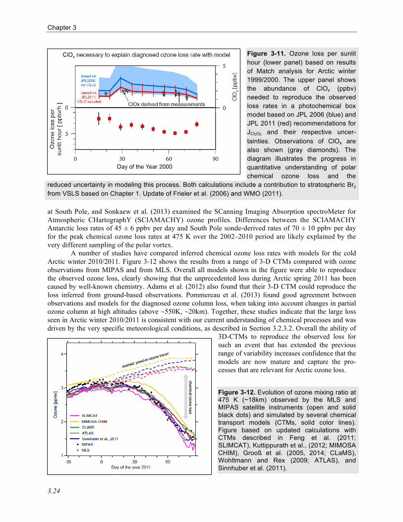
Chapter 3

 3.24

Figure 3-11. Ozone loss per sunlit hour (lower panel) based on results of Match analysis for Arctic winter 1999/2000. The upper panel shows the abundance of ClOx (ppbv) needed to reproduce the observed loss rates in a photochemical box model based on JPL 2006 (blue) and JPL 2011 (red) recommendations for JCl2O2 and their respective uncer-tainties. Observations of ClOx are also shown (gray diamonds). The diagram illustrates the progress in quantitative understanding of polar chemical ozone loss and the

reduced uncertainty in modeling this process. Both calculations include a contribution to stratospheric Bry from VSLS based on Chapter 1. Update of Frieler et al. (2006) and WMO (2011).

at South Pole, and Sonkaew et al. (2013) examined the SCanning Imaging Absorption spectroMeter for Atmospheric CHartographY (SCIAMACHY) ozone profiles. Differences between the SCIAMACHY Antarctic loss rates of 45 ± 6 ppbv per day and South Pole sonde-derived rates of 70 ± 10 ppbv per day for the peak chemical ozone loss rates at 475 K over the 2002–2010 period are likely explained by the very different sampling of the polar vortex.

A number of studies have compared inferred chemical ozone loss rates with models for the cold Arctic winter 2010/2011. Figure 3-12 shows the results from a range of 3-D CTMs compared with ozone observations from MIPAS and from MLS. Overall all models shown in the figure were able to reproduce the observed ozone loss, clearly showing that the unprecedented loss during Arctic spring 2011 has been caused by well-known chemistry. Adams et al. (2012) also found that their 3-D CTM could reproduce the loss inferred from ground-based observations. Pommereau et al. (2013) found good agreement between observations and models for the diagnosed ozone column loss, when taking into account changes in partial ozone column at high altitudes (above ~550K, ~20km). Together, these studies indicate that the large loss seen in Arctic winter 2010/2011 is consistent with our current understanding of chemical processes and was driven by the very specific meteorological conditions, as described in Section 3.2.3.2. Overall the ability of

3D-CTMs to reproduce the observed loss for such an event that has extended the previous range of variability increases confidence that the models are now mature and capture the pro-cesses that are relevant for Arctic ozone loss.

Figure 3-12. Evolution of ozone mixing ratio at 475 K (~18km) observed by the MLS and MIPAS satellite instruments (open and solid black dots) and simulated by several chemical transport models (CTMs, solid color lines). Figure based on updated calculations with CTMs described in Feng et al. (2011; SLIMCAT), Kuttippurath et al., (2012; MIMOSA CHIM), Grooß et al. (2005, 2014; CLaMS), Wohltmann and Rex (2009; ATLAS), and Sinnhuber et al. (2011).

Polar Ozone

 3.25

3.3.3 Polar Dynamical Processes

3.3.3.1 RELATION BETWEEN WAVE DRIVING AND POLAR OZONE

Ozone inside the polar vortex and in the collar region surrounding the polar vortex experiences large year-to-year variations (WMO, 2011). The main driver for this variability is variations in atmospheric dynamics (Fusco and Salby, 1999; Randel et al., 2002; Weber et al., 2003, 2011; Hood and Soukharev, 2005; Salby, 2008). Variability in the planetary wave activity driving the winter Brewer-Dobson circulation modulates both dynamical and chemical processes affecting polar ozone (e.g., Tegtmeier et al., 2008). The links between planetary waves and polar ozone losses results from the temperature modulation (e.g., Newman et al., 2001). Mass circulations associated with momentum deposition by the planetary waves leads to adiabatic compression of polar air masses (and immediate warming, e.g., SSWs (Ayarzaguëna et al., 2011)) and expansion in the tropical lower stratosphere (cooling). The return toward radiative equilibrium (slow diabatic cooling) in the polar region then results in enhanced transport into the polar vortex and subsidence inside the vortex area. The combination of enhanced transport and warmer polar temperatures in a given winter is then responsible for higher polar ozone levels, reduced polar ozone losses, and leads to higher spring total ozone (e.g., Chipperfield and Jones, 1999; de Laat and van Weele, 2011; Kuttipurath et al., 2010b; Kuttipurrath and Nikulin, 2012; Kramarova et al., 2014). Our understanding of the mechanisms that determine the degree of wave driving of the polar stratosphere is still incomplete, but some progress has been made.

Weber et al. (2011) showed a compact relationship between the mean winter eddy heat flux at 100 hPa, a measure for the planetary wave activity and BDC strength, and spring-to-fall polar ozone ratio combining data from both hemispheres (Figure 3-13). The planetary wave activity is much lower in the Southern Hemisphere and, therefore, results in spring-to-fall ozone ratios smaller than 1 (polar ozone loss outweighs ozone transport). In the Northern Hemisphere this ratio is always above 1 (ozone transport outweighs polar ozone loss). The various extreme events like the split of the Antarctic vortex in 2002 (with an

ozone ratio above 1), the record Antarctic ozone hole in 2006, the cold Arctic winters in 1996, 1997, and 2011 (e.g., Manney et al., 2011), and high Arctic ozone in 2010 (Steinbrecht et al., 2011) follow this compact linear relationship.

Figure 3-13. Spring-to-fall ratio of observed polar cap total ozone (>50°) as a function of the absolute extra-tropical winter mean eddy heat flux (September to March in the Northern Hemi-sphere and March to September in the Southern Hemisphere) derived from ECMWF ERA-Interim data. Data from the Southern Hemisphere are shown as triangles (September over March ozone ratios) and from the Northern Hemisphere as solid circles (March over September ratios). Selected polar total ozone distributions for selected years are shown at the top. Updated from Weber et al. (2011).

Chapter 3

 3.26

This linear relationship between eddy heat flux and polar cap ozone was also found in two CCMs, indicating that current models realistically describe the variability in stratospheric circulation and its effect on total ozone (Weber et al., 2011). Both models show a positive trend in the winter mean eddy heat flux (and winter BDC strength) in both hemispheres until year 2050, however, the interannual variability (peak-to-peak) is two to three times larger than the change in the decadal means between 1960 and 2050 (Weber et al., 2011). Substantial polar ozone losses could occur in the case of particularly cold winters in the coming decades despite the ongoing decrease of ODS levels in the stratosphere.

3.3.3.2 THE ROLE OF LEADING MODES OF DYNAMICAL VARIABILITY

The respective influences of natural variability and anthropogenic climate change on polar stratospheric temperatures are difficult to disentangle given the short observational record in the satellite era. Using reanalyses and radiosonde data, Bohlinger et al. (2014) showed a wintertime positive trend in Arctic temperatures at 50 hPa over the past three decades, and a corresponding increase in planetary wave activity diagnosed as the meridional eddy heat fluxes at 100 hPa. In addition, they have identified a residual radiative cooling trend of about −0.5 K/decade. Nevertheless, the processes in the troposphere that govern the large interannual variability and the trend in these temperatures remain to be fully understood. It is particularly important to understand the origin of very strong vortex events that drive the ozone loss, either short-duration intense cooling episodes as observed in January 2010 (Dörnbrack et al., 2012), or else prolonged coolings like that observed during the late winter and spring 2011 (Manney et al., 2011). Several recent observational studies have shown that tropospheric highs (e.g., blockings) can lead to either warming or cooling of the Northern Hemisphere polar stratosphere, depending upon their geographical location (Nishii et al., 2011; Woollings et al., 2010; Castanheira and Barriopedro, 2010). This dual effect arises from the potential interaction of transient waves with climatological planetary waves, thereby increasing or lowering the wave activity flux into the stratosphere. North Pacific blockings distinctly lead to polar stratospheric coolings (Nishii et al., 2010), and brief vortex cooling episodes observed during the 2009/10 (Dörnbrack et al., 2012). Also the 2010/2011 winter, described in Section 3.2.3.2, was clearly associated with North Pacific highs and a precursory enhanced Western Pacific teleconnection pattern (Orsolini et al., 2009). The exact cause of the prolonged cold stratosphere in March and April 2011, which led to the record ozone loss, remains unclear, but may involve complex dynamical positive feedbacks between a small intense polar vortex and equatorward-deflected planetary waves. Recent observational and modeling studies emphasize the role of a warm anomaly in North Pacific sea surface temperatures in leading to the cold vortex in 2011 (Hurwitz et al., 2011, 2012). Hence, a better understanding of the variability of the coupled ocean-atmosphere circulation not only in the North Atlantic but also in the key Eastern Eurasia/North Pacific region where wave activity fluxes into the stratosphere are climatologically the strongest, may lead to a better understanding of polar stratospheric temperature variability.

Kiesewetter et al. (2010) showed that the stratospheric Northern Annular Mode (NAM) index is strongly correlated with Arctic ozone anomalies. The different phases of the NAM are driven by the variability in planetary wave driving. Extreme phases of the NAM index (strong and weak vortex events) are associated with negative and positive ozone anomalies that descend from the uppermost stratosphere and then rapidly cover the upper and middle stratosphere, from where they then slowly descend into the lowermost stratosphere within 5 months.

Another important factor in modulating the strength of the polar vortices is the equatorial quasi-biennal oscillation (QBO). The QBO influences the propagation of waves, e.g., during QBO easterlies the waves are more directed toward the polar region, decelerating the polar night jet and perturbing the polar vortex (Holton and Tan, 1980; Baldwin et al., 2001; Naoe and Shibata, 2010; Anstey and Shepherd, 2014; Watson et al., 2014). There is a close link between the QBO and the occurrence of SSWs and the date of the final warming (Thiéblemont et al., 2011). Similarly, planetary wave activity tends to be stronger during warm phases of the El Niño-Southern Oscillation (ENSO) (e.g., Garfinkel and Hartmann, 2008).

Polar Ozone

 3.27

Trends and changes in the amplitude of Southern Hemisphere stationary waves in reanalyses are associated with polar ozone depletion and changes in the strength of the subtropical jets driven by sea surface temperature (SST) forcing (Wang et al., 2013; Agosta and Canziani, 2011). Sonkaew et al. (2013) showed that the variable Arctic ozone loss as determined from SCIAMACHY limb ozone profiles during 2002–2009 correlate with the QBO phase, meaning larger ozone losses were generally observed during QBO west phases, although the studied period is relatively short. Hurwitz et al. (2011) showed that the dynamical conditions prevailing during Arctic winter 2011 were characterized as expected by a QBO westerly phase and a concurrent La Niña phase. However, these features alone cannot explain the persistence of the low temperature anomaly into March 2011. As mentioned above, they identified the positive North Pacific SST anomaly as a potential driver for the cold Arctic vortex in late winter 2011.

3.3.3.3 MERIDIONAL MIXING

Blessmann et al. (2012a) showed that a larger fraction of ozone from lower latitudes is mixed into the Arctic vortex in early winter when the wave activity in late fall has been high. In the contrasting case of low wave activity, a larger fraction of early winter polar vortex ozone has subsided from the upper stratosphere during fall. The amount and variability (10%) of early winter Arctic ozone below 750 K (~30 km) are largely determined by dynamical processes in the early vortex formation period (Blessmann et al., 2012b).

Using ozone observations above Antarctica in combination with a CTM model, Roscoe et al. (2012) confirmed earlier studies that the polar ozone depletion starts earlier for stations that are closer to the vortex edge than those in the core region. They also showed from dynamical considerations that air parcels from the core region and the vortex edge region mix only weakly. As the vortex edge region is more strongly exposed to sunlight and is generally warmer, a cooling trend in the stratosphere could extend the region where PSC formation is possible, potentially delaying ozone recovery. This contrasts to the core region where the formation of PSCs is saturated and is less impacted by additional cooling.

3.4 RECOVERY OF POLAR OZONE

Detection of polar ozone recovery is an important milestone in assessing the effectiveness of the Montreal Protocol. As indicated in Chapter 1 of this assessment, the stratospheric chlorine and bromine burden as expressed by the Equivalent Effective Stratospheric Chlorine (EESC) has decreased by about 10% in the polar regions from its peak level reached in the beginning of this century. This section assesses whether an increase in ozone is observed in the polar regions that can be attributed to the decrease in ODSs. Recent changes in understanding of polar ozone trends are discussed in the context of what has been discussed in previous assessments. The focus is on observed polar ozone changes. Future polar ozone evolution is discussed in detail in Section 3.5.

3.4.1 Polar Ozone Recovery in Previous Assessments

The WMO/UNEP 2006 Ozone Assessment Report (WMO, 2007; see Section 6.2.2) outlined in detail the different stages of current and future ozone: slowdown of ozone decline, turn around and onset of ozone increases, and full recovery from ODSs. The latter will be discussed in the context of future polar ozone in Section 3.5. WMO (2007) established that slowing and cessation of ozone decline had already occurred and that 1997 was the most likely turnaround year. That report also included predictions of a slow recovery of Antarctic column ozone, with an increase in springtime ozone of 5–10% between 2000 and 2020, or 0.25–0.5%/year over that period.

The WMO/UNEP 2010 Ozone Assessment Report (WMO, 2011) firmly established that for detection of the second stage of ozone recovery—the occurrence of statistically significant increases in ozone above previous minimum values due to declining EESC—it is required to separate dynamical from

Chapter 3

 3.28

chemical influences on ozone (Newman et al., 2006; Yang et al., 2008). A standard approach for detection that was discussed in WMO (2011, see Section 2.1.2; Box 3-2) is to use a multivariate regression model that quantifies the relation between ozone and different dependent variables that simultaneously describe natural and anthropogenic forcings. The long-term trend can either be described by fitting a piece-wise linear trend function (PWLT) or the EESC. For the PWLT, the turning point is typically defined at the EESC maximum. Alternatively, the turning point can also be derived from a break-point analysis of the ozone record (Yang et al., 2005, 2008; Chehade et al., 2014).

WMO (2011) also discussed the available regression studies, which at that time had focused on tropical and midlatitude ozone. However, analyzing polar ozone for long-term trends and signs of onset of ozone increases had not been performed before WMO (2011), as it is more complicated due to the need to include polar vortex dynamics, which results in larger year-to-year variability in polar regions than at midlatitudes and in the tropics. In WMO (2011), Antarctic trends were only briefly discussed, as essentially only one regression study was available at the time (Yang et al., 2008). Furthermore, that study only considered temperature as a dependent variable and focused on the first stage of ozone recovery, the leveling off of Antarctic ozone loss and reversal of the EESC trend from increasing during the 1980s and 1990s to a decrease after 2000. It was concluded that the leveling off of Antarctic ozone since the late 1990s could be attributed to changes in Antarctic stratospheric halogen loading.

In addition, WMO (2011) noted based on model studies that increases in greenhouse gas (GHG) concentrations do not have a significant direct effect (due to radiative processes) on springtime Antarctic polar temperatures and ozone for the period up to 2100. Indirect effects of GHG on ozone via changes in vortex dynamics were not reported in WMO (2011). Furthermore, there are large uncertainties associated with the ozone recovery path, and model uncertainties rather than those of GHG scenarios dominate uncertainties in ozone recovery. Hence, it is unlikely that recent Antarctic stratospheric ozone changes were affected by increases in GHGs. See further Section 3.5 on the impact of GHGs on future Antarctic ozone recovery.

For the Arctic, WMO (2007) already noted that compared to the Antarctic, the Arctic shows larger interannual variability in springtime ozone and smaller ozone depletion. As a result, detection of changes in ozone due to decreases in EESC will likely take longer than in the Antarctic. For the Arctic, no slowing of a decline in ozone had been found. WMO (2011) reported little progress in assessing Arctic ozone recovery since WMO (2007).

3.4.2 Long-Term Antarctic Ozone Trends

3.4.2.1 VERTICALLY RESOLVED OZONE

Hassler et al. (2011a) assessed 25 years of ozonesonde measurements made at the South Pole station and presented an update and expansion of earlier South Pole ozonesonde studies (Hofmann et al., 1997; Solomon et al., 2005; Hofmann et al., 2009). The study analyzed the height dependence of ozone loss rates throughout Antarctic spring (late August to late September) for five-year periods, which reduces the effect of year-to-year variability in ozone (Figure 3-14). The study concluded that ozone loss rates changed little over the period 1996–2010, although a small but statistically insignificant reduction in ozone loss rates after 2000 was identified. The lack of clear reduction in ozone loss rates (Figure 3-14) could be partly related to saturation of loss at certain pressure levels which results in the near-complete ozone destruction at pressure levels around 70 hPa (typically 50–100 hPa; see also Yang et al. (2008)). It thus may take some time for air masses at certain pressure levels to become “desaturated” with regard to ozone loss. Furthermore, the decrease in EESC during the period 2000–2010 is approximately 5–10%, depending on the choice of age of air (Newman et al., 2007), suggesting that no large decrease in ozone destruction can be expected to have occurred yet. Assuming a future linear relation between the reduction in EESC and ozone loss rates and assuming that future dynamical variability of the Antarctic stratosphere will remain similar to the variability observed during the last two decades as well as assuming that no

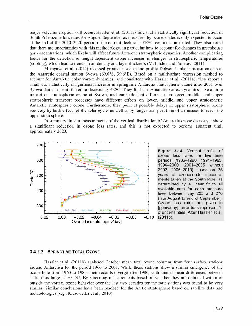
Polar Ozone

 3.29

major volcanic eruption will occur, Hassler et al. (2011a) find that a statistically significant reduction in South Pole ozone loss rates for August–September as measured by ozonesondes is only expected to occur at the end of the 2010–2020 period if the current decline in EESC continues unabated. They also noted that there are uncertainties with this methodology, in particular how to account for changes in greenhouse gas concentrations, which likely will affect future Antarctic stratospheric dynamics. Another complicating factor for the detection of height-dependent ozone increases is changes in stratospheric temperatures (cooling), which lead to trends in air density and layer thickness (McLinden and Fioletov, 2011).

Miyagawa et al. (2014) assessed ground-based ozone profile Dobson Umkehr measurements at the Antarctic coastal station Syowa (69.0°S, 39.6°E). Based on a multivariate regression method to account for Antarctic polar vortex dynamics, and consistent with Hassler et al. (2011a), they report a small but statistically insignificant increase in springtime Antarctic stratospheric ozone after 2001 over Syowa that can be attributed to decreasing EESC. They find that Antarctic vortex dynamics have a large impact on stratospheric ozone at Syowa, and conclude that differences in lower, middle, and upper stratospheric transport processes have different effects on lower, middle, and upper stratospheric Antarctic stratospheric ozone. Furthermore, they point at possible delays in upper stratospheric ozone recovery by both effects of the solar cycle, as well as by longer transport time of air masses to reach the upper stratosphere.

In summary, in situ measurements of the vertical distribution of Antarctic ozone do not yet show a significant reduction in ozone loss rates, and this is not expected to become apparent until approximately 2020.

Figure 3-14. Vertical profile of ozone loss rates for five time periods (1986–1990, 1991–1995, 1996–2000, 2001–2005 without 2002, 2006–2010) based on 25 years of ozonesonde measure-ments taken at the South Pole, as determined by a linear fit to all available data for each pressure level between day 235 and 270 (late August to end of September). Ozone loss rates are given in [ppmv/day], error bars represent 1-σ uncertainties. After Hassler et al. (2011b).

3.4.2.2 SPRINGTIME TOTAL OZONE

Hassler et al. (2011b) analyzed October mean total ozone columns from four surface stations around Antarctica for the period 1966 to 2008. While these stations show a similar emergence of the ozone hole from 1960 to 1980, their records diverge after 1980, with annual mean differences between stations as large as 50 DU. By screening measurements based on whether they are obtained within or outside the vortex, ozone behavior over the last two decades for the four stations was found to be very similar. Similar conclusions have been reached for the Arctic stratosphere based on satellite data and methodologies (e.g., Kiesewetter et al., 2010).

Chapter 3

 3.30

Salby et al. (2011, 2012) presented the first claim of detection of the second phase of recovery of Antarctic ozone, i.e., a statistically significant increase in ozone due to declining EESC. They applied a two-parameter regression model to analyze annual springtime (September–November) Total Ozone Mapping Spectrometer (TOMS)/OMI total ozone over Antarctica poleward of 70°S (vortex core). Total ozone measurements were regressed against the upward Eliassen-Palm (EP) flux at 70 hPa, averaged poleward of 40°S during the period August–September, and the QBO, represented by tropical 30 hPa winds. Salby et al. (2011) reported a correlation (R2) of springtime vortex core total ozone variations by their two-parameter regression model of 0.96. By applying these regressions, dynamical processes that determine year-to-year variability in Antarctic vortex strength and ozone destruction can be removed from the total ozone record, leaving an ozone residual that can be probed for the presence of trends. A positive linear trend for the period 1996–2008 was reported with a statistical significance of 99.5% using a two-tailed t-test. Note that the results from Salby et al. (2011, 2012) cannot directly be compared to those of Hassler et al. (2011a), in part because they look at different springtime periods, and also because Salby et al. (2011, 2012) investigate a vortex-average total ozone amount, whereas Hassler et al. (2011a) investigate ozone profiles taken at one specific location.

Kuttippurath et al. (2013) presented more extensive multivariate regression analyses of Antarctic polar vortex total ozone for the period 1979–2010. They analyzed two different satellite total ozone data sets (TOMS/OMI and MSR), as well as averaged ground-based Antarctic measurements of total ozone. They further applied the multivariate regression to three total ozone time series based on three different Antarctic ozone records: average total ozone inside the vortex and the vortex core, both based on passive tracer transport model simulations, as well as average total ozone for equivalent latitudes between 65° and 90°S. Finally, they applied two different trend estimates to the total ozone time series: either the EESC or PWLT were used as fit parameters in the multivariate regression. Trends were calculated for the periods both before and after 2000. The multivariate regression model includes effects of the solar flux, QBO, stratospheric aerosols, the heat flux (or Eliassen-Palm flux), and the Antarctic oscillation (or Southern Annular Mode). Taking these effects into account, the three types of measurements, the three vortex definitions, and the two linear trend methods all show a statistically significant positive trend in Antarctic total ozone for the period 2000–2010. The recovery rates based on the PWLT trend estimates are approximately 25 DU/decade or 8%/decade, while the EESC fit provides an estimate of approximately 10 DU/decade or 3%/decade. Both trend estimates are significant at the 95% confidence level. Differences between PWLT and EESC trend estimates indicate that vortex dynamics are important and should be considered, consistent with findings from Kiesewetter et al. (2010) and Hassler et al. (2011a).

The correlation of the multivariate regression in Kuttipurrath et al. (2013) does not exceed 0.90 (R2), which appears inconsistent with the 0.96 (R2) correlation found by Salby et al. (2011), despite the latter study being based on only two dependent variables. The cause of this discrepancy is currently unclear, but it should be kept in mind that although both studies include the same dependent variables (QBO and heat flux), they use different underlying base data (40 hPa tropical wind speed QBO and ECMWF ERA Interim heat flux in Kuttippurath et al. (2013); 30 hPa wind speed QBO and NCEP heat flux in Salby et al. (2011, 2012)). The time period over which total ozone data are averaged is also different (between September and November in the former case, over October in the latter case), as well as the length of the period under consideration (1996–2008 for Salby et al. (2011, 2012), and 2000–2010 for Kuttippurath et al. (2013)). In addition, these studies do not address several other sources of uncertainty, like regression parameter choices, regressor errors, and sensitivity to the time period over which the regressors are taken.

In summary, although findings of multivariate regression studies of springtime Antarctic total ozone are consistent with a beginning of ozone recovery, i.e., they report increases in ozone after 2000, uncertainties in measurements and regressors as well as uncertainties in statistical analyses preclude the definitive conclusion that Antarctic stratospheric ozone is increasing due to declining ODSs.

Polar Ozone

 3.31

3.4.3 Long-Term Ozone Trend in the Arctic

Previous WMO/UNEP Ozone Assessments have noted that the large degree of interannual variability in meteorological conditions, and the strong dependence on the start and end dates used for the analysis render robust determination of ozone trends in the Arctic extremely problematic. The picture remains largely unchanged for this Assessment. Although several studies have placed the exceptional 2011 Arctic spring ozone values in context through comparisons with multiyear (in some cases multidecade) ozone data sets (Manney et al., 2011; Balis et al., 2011; Hurwitz et al., 2011; Arnone et al., 2012; Adams et al., 2012; Kuttippurath et al., 2012; Lindemaier et al., 2012; Isaksen et al., 2012; Pommereau et al., 2013; Strahan et al., 2013), few have specifically quantified long-term changes in Arctic lower stratospheric ozone. It is thus not possible to make a definitive statement about Arctic ozone trends at this time.

3.5 FUTURE CHANGES IN POLAR OZONE

Future changes in ozone can be assessed with models of varying complexity (parametric, two- and three-dimensional models). In recent years the state-of-the-art for assessing stratospheric ozone changes in a climate context has moved to comprehensive three-dimensional chemistry-climate models (CCMs). A major milestone for the CCM community was the CCMVal-2 model intercomparison report (SPARC CCMVal, 2010) that preceded the WMO/UNEP 2010 Ozone Assessment (WMO, 2011) and informed the conclusions therein. Progress with CCMs since has been continuous and new studies have either consolidated or added details to results from CCMVal-2. No recent study has challenged our fundamental understanding of how ozone will develop in the future, based on decreasing ODSs and continued evaluation of climate change sensitivities.

No intercomparison on the scale of CCMVal-2 has been carried out in time for this Ozone Assessment. The SPARC lifetime assessment (SPARC, 2013) has reassessed lifetimes of a number of ODSs using observations and models. The CCMs that contributed to the modeling part of the lifetime assessment have been updated since CCMVal-2 and will be used for future integrations and collaborative efforts, including the Chemistry-Climate Model Initiative (CCMI). Even though the modeling part of the lifetime assessment is extremely valuable for attributing past ozone changes by providing additional model integrations covering the recent past, it is investigating time-slice experiments for the future (Chipperfield et al., 2014), which are not directly comparable to the transient integrations projecting 2100 ozone levels in CCMVal-2. However, changed lifetimes of ODSs can be used in an indicative way and in updated model integrations. If key lifetimes are significantly increased, projected ozone recovery will be delayed. Table 6.1 in SPARC (2013) summarizes the new lifetimes for CFC-11 and CFC-12, among others. The recommended lifetimes increased from 45 to 52 years for CFC-11 and from 100 to 102 years for CFC-12. This lifetime adjustment does not suggest a major change of return and recovery dates reported in WMO (2011). Commonly the lifetime information of a species is used in conjunction with the assumed surface fluxes to calculate surface mixing ratios. The time-dependent surface mixing ratios are subsequently used as boundary conditions for CCM integrations. Four CCMs used in CCMVal-2 (SPARC CCMVal, 2010) and subsequently presented in WMO (2011), i.e., CMAM, GEOSCCM, UMSLIMCAT, and WACCM, compared the impact of changing from the WMO (2011) mixing ratio time series of ODSs to the SPARC (2013) recommendations (Figure 3-15). In Figure 3-15 the thick black line is the multi-model mean (MMM) polar total ozone from the four CCMs as contributed to WMO (2011) using Special Report on Emissions Scenarios (SRES) A1B scenario for well-mixed GHG and the WMO (2011) recommended ODS concentrations. The thin colored lines are pairwise differences added to the MMM for each of the four models. The models used Representative Concentration Pathway (RCP) 6.0 (GEOSCCM, WACCM, and CMAM) or RCP 4.5 (UMSLIMCAT) scenarios for well-mixed GHG in the updated runs. The turquoise shading is the one standard deviation interannual variability for March or October respectively added/subtracted to the MMM. Note that the differences are small and that they lie

Chapter 3

 3.32

     

Figure 3-15. The thick black line is showing multi-model mean (MMM) polar total ozone (60°-90°; left: Northern Hemisphere March, right: Southern Hemisphere October) from four CCMs (see legend) that contributed to WMO (2011) using SRES A1B for well-mixed GHG and the WMO (2011) recommended ODS concentrations. The thin colored lines are pairwise differences (“old-new” ODS scenarios; “old”: WMO, 2011; “new”: SPARC, 2013) added to the MMM for each of the four models. The “new” integrations used RCP 6.0 (CMAM, GEOSCCM, and WACCM) or RCP 4.5 (UMSLIMCAT) for well-mixed GHG. The turquoise shading is the one standard deviation interannual variability for March (left) and October (right) from GEOSCCM added/subtracted to the MMM. Horizontal dashed lines are 1980 values. largely within the one standard deviation range, thus suggesting that the ODS lifetime change had no significant impact on the polar ozone recovery in either the Northern or Southern Hemisphere. However it should be noted that this “by chance ensemble” provides a MMM that is returning late to 1980s ozone values in the Southern Hemisphere, compared to the full WMO (2011) MMM.

3.5.1 Factors Controlling Polar Ozone Amounts

Section 3.3 describes our level of understanding of processes influencing polar ozone changes. CCMs are an attempt to utilize this process understanding to simulate (in a comprehensive way) chemistry-climate interactions, allowing us to make projections into the future. Such models are of increasing complexity (e.g., consider more and more Earth system components with higher complexity). Like all models, CCMs have to compromise in terms of complexity and resolution, to provide the length of integrations required to evaluate interactions between composition and climate on longer timescales. Continuous validation of the model performance for the recent past is a key to our judgment of model projections, even though good model performance for the past does not necessarily guarantee reliable predictions.

Two main factors determine future ozone amounts: How fast are the stratospheric chlorine and bromine amounts changing, and what is the impact of increasing GHGs on ozone? Box 3-2 summarizes many important aspects relating to this issue. To illustrate the success of the Montreal Protocol, it is useful to consider so-called “world avoided” simulations. Since the last Assessment, Garcia et al. (2012) used an updated version of the Whole Atmosphere Community Climate Model (WACCM) model, illustrating the expected strong impact of heterogeneous chemistry on the ozone budget and quantifying the ozone loss avoided by the Montreal Protocol. Their results are in good agreement with earlier studies that have been reported in WMO (2011).

For tracing the success of the Montreal Protocol, previous WMO/UNEP ozone assessments have introduced the concepts of ozone recovery and return. As emphasized in Section 3.4, ozone recovery relates to the physical effects ODSs have on stratospheric ozone. When ODSs no longer significantly

Polar Ozone

 3.33

affect ozone chemistry, full ozone recovery has been achieved. For this consideration, transport effects, e.g., the removal of chlorine-containing species from the stratosphere, are most important (indicated with a downward pointing arrow in Box 3-2).

Return relates to the achievement of a threshold ozone amount that was observed in the past. When ODS abundances decline in the stratosphere, ozone will increase. In addition ozone will increase due to a cooling of the upper stratosphere that is caused by increasing GHGs (Box 3-2). Simultaneously, changes in meridional transport would modify the high-latitude ozone budget, with current CCMs indicating a strengthening of the BDC for GHG increases. This has been extensively discussed in WMO (2011) and it was concluded that, “A stronger BDC would decrease the abundance of tropical lower stratospheric ozone, increase poleward transport of ozone, and could reduce the atmospheric lifetimes of long-lived ODSs and other trace gases.” A detailed discussion of the recent findings regarding the evolution of the BDC is presented in Chapter 4 of the present Assessment.

Baumgaertner et al. (2010) add a nuance to the general picture by pointing out that upper stratospheric NOx enhancement due to a stronger BDC would cause additional ozone loss, but that the ozone loss would be more or less canceled by more poleward ozone transport. The added effects of decreasing ODSs, increasing GHGs, and changing meridional transport will lead to polar ozone return dates that are earlier than the recovery dates. Arguably the evolution of return dates, in particular in total ozone, is more straightforward and easier to measure than the exact timing of recovery.

Even though two important factors determining future ozone are well understood, namely, the ozone change due to decreasing ODSs and the stratospheric cooling due to GHGs, many mechanisms exist that are uncertain in their future development. One of the uncertainties lies with the PSCs (Box 3-2). How will they develop under climate change? Will there be more PSCs due to radiatively controlled cooling, or less due to dynamically induced warming? Hurwitz and Newman (2010) looked at the development of the PSC area in projections using the Goddard Chemistry-Climate Model (GEOSCCM). In their model, future trends in the PSC area in October over Antarctica were negative, thus “helping” ozone return. In addition, Deushi and Shibata (2011) investigated the impact of GHGs on ozone recovery. In their model, resolved wave forcing is decreased in spring over Antarctica, due to an earlier breakdown of the polar vortex in the future. If this is a verifiable result, it would indicate a potential mechanism for earlier ozone return dates. More examples are discussed in Sections 3.3.3 and in 3.5.3.1.

3.5.2 Long-Term Projection of Polar Ozone Amounts

A multi-model mean (MMM) total ozone time series relative to a particular year is a relatively robust representation of an “average” behavior for the future. An uncertainty range can be described by the inter-model standard deviation that is usually large. The large standard deviations arise because the models are potentially biased and their meteorology will differ in the same nominal year. However each individual model ozone time series is referenced to its own climatological base period. Therefore a large spread does not mean that models disagree on the general temporal development of ozone. The spread is merely highlighting that the models differ.

Following considerations in Austin et al. (2010a) and WMO (2011), Figure 3-16 presents a MMM anomaly total ozone time series. In Figure 3-16, 1980 ozone values are indicated with a dashed line. The thick red line indicates the MMM total ozone anomaly for the Arctic in March (Figure 3-16, top) and for Antarctica in October (Figure 3-16, bottom). The spread is indicated by a two standard deviation interval (gray shading). The MMM time series indicate an earlier return date with respect to 1980 values for the Arctic (near 2030) than for the Antarctic (near 2050). Note that the CCMVal-2 integrations have been performed with a particular Special Report on Emission Scenario (SRES) climate changes scenario (A1B). For the recent IPCC report (AR5; IPCC, 2013), SRES scenarios have been superseded by Representative Concentration Pathways (RCP) scenarios (van Vuuren et al., 2011). Both SRES and RCP are descriptions of the possible evolution of climate forcings that depend on assumptions, e.g., how energy consumption will develop in the future, and a range of possibilities is considered. This scenario

Chapter 3

 3.34

Box 3-2. Factors Determining Future Polar Ozone Ozone-depleting substances (ODSs) are the drivers of polar ozone loss. Due to the Montreal Protocol and

its Amendments, ODS amounts are decreasing and ozone will recover. Here, we discuss factors that influence details of the recovery process. Factors influencing future ozone amounts in high latitudes at different heights are: changes in meridional transport (indicated by bold open arrows), temperature changes from increased long-lived GHGs (indicated by blue or red shaded areas), and chemical effects (the future potential to form PSCs that can activate available halogens, e.g., chlorine and to a lesser extent bromine, and changes in temperature-dependent reaction rates). Each effect is changing ozone at certain heights. A combination of all effects is manifested in the total ozone, the vertically integrated amount of ozone.

The sketch below shows polar latitudes (with the North or South Pole to the left) versus altitude. The altitude scale is roughly indicated by the position of the polar tropopause (black dashed line). Stratospheric cooling and tropospheric warming are indicated with color-shaded areas. Poleward transport and generally descending motion, as well as air exchange between the stratosphere and the troposphere, are indicated with bold open arrows. The blue half ellipse shows the region where PSCs occur when temperatures are low enough. The green half ellipse denotes the ozone maximum in partial pressure or number density.

Changes in transport under climate change: Models predict a strengthening of the Brewer-Dobson circulation (BDC) for increased long-lived GHG concentrations. Increased poleward transport would provide a gain in polar ozone. Increased downward transport and more efficient air exchange between the stratosphere and the troposphere would provide a more efficient removal mechanism for halogen-containing species, the main driver of ozone destruction.

Changes in temperature under climate change: The increase of long-lived GHGs has led to a warming in the troposphere and cooling in the stratosphere. Many processes and reactions that change ozone are temperature dependent. In colder conditions more PSCs could be formed, thus providing a greater potential for halogen activation and ozone destruction. Furthermore, PSC formation depends on the availability of water vapor; future trends in water vapor are uncertain.

Chemical effects: They are closely coupled to the transport and temperature changes. In the lower stratosphere they depend on the availability of halogen-containing species and the occurrence, amount, and timing of PSCs. In the upper stratosphere, chlorine chemistry also plays a role. However, lower temperatures there slow down the gas-phase destruction of ozone, thus resulting in more ozone. In addition, changes in N2O and CH4 concentrations could affect ozone chemistry as well.

Because all effects above contribute to changes in polar total ozone, it is more difficult to monitor total ozone recovery than return. Total ozone recovery relies on the concept that ozone amounts are no longer significantly affected by halogen chemistry and full recovery would imply that halogens of anthropogenic origin no longer play a role in determining ozone amounts. Total ozone return is a simpler milestone to monitor, answering the question “When do we reach a level of ozone that we had in the past?”

Altitud

e  

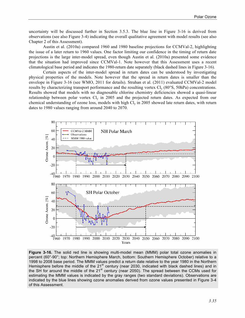
Polar Ozone

 3.35

uncertainty will be discussed further in Section 3.5.3. The blue line in Figure 3-16 is derived from observations (see also Figure 3-4) indicating the overall qualitative agreement with model results (see also Chapter 2 of this Assessment).

Austin et al. (2010a) compared 1960 and 1980 baseline projections for CCMVal-2, highlighting the issue of a later return to 1960 values. One factor limiting our confidence in the timing of return date projections is the large inter-model spread, even though Austin et al. (2010a) presented some evidence that the situation had improved since CCMVal-1. Note however that this Assessment uses a recent climatological base period and indicates the 1980-return date separately (black dashed lines in Figure 3-16).

Certain aspects of the inter-model spread in return dates can be understood by investigating physical properties of the models. Note however that the spread in return dates is smaller than the envelope in Figure 3-16 (see WMO, 2011 for details). Strahan et al. (2011) evaluated CCMVal-2 model results by characterizing transport performance and the resulting vortex Cly (80°S, 50hPa) concentrations. Results showed that models with no diagnosable chlorine chemistry deficiencies showed a quasi-linear relationship between polar vortex Cly in 2005 and the projected return dates. As expected from our chemical understanding of ozone loss, models with high Cly in 2005 showed late return dates, with return dates to 1980 values ranging from around 2040 to 2070.

Figure 3-16. The solid red line is showing multi-model mean (MMM) polar total ozone anomalies in percent (60°-90°; top: Northern Hemisphere March, bottom: Southern Hemisphere October) relative to a 1998 to 2008 base period. The MMM values predict a return date relative to the year 1980 in the Northern Hemisphere before the middle of the 21st century (near 2030, indicated with black dashed lines) and in the SH for around the middle of the 21st century (near 2050). The spread between the CCMs used for estimating the MMM values is indicated by the gray ranges (two standard deviations). Observations are indicated by the blue lines showing ozone anomalies derived from ozone values presented in Figure 3-4 of this Assessment.

Observations

Chapter 3

 3.36

3.5.3 Uncertainties of Future Polar Ozone Changes

We can distinguish three different contributors to uncertainty: internal variability of the atmosphere, model uncertainty, and scenario uncertainty. Depending on the quantity, internal variability can be a small or large source of uncertainty. In contrast model uncertainty is commonly significant. Scenario uncertainty is less problematic in the near future (e.g., for the next twenty years), because different RCPs diverge more for the far future than for the near future. Consequently scenario uncertainty increases rapidly for the later decades, because we do not know which path will be chosen in the far future.

Charlton-Perez et al. (2010) estimated uncertainty contributions in multi-model mean projections of annual and global mean total ozone. They use global and annual mean data to keep the contribution of internal variability small. The spatial and temporal averaging mitigates the magnitude of internal variability that would be far more dominant for, e.g., seasonal or monthly mean data. Indications are that scenario uncertainties are increased in the late 21st century with RCP (used in Coupled Model Intercomparison Project Phase 5, CMIP5) compared to SRES A1B (used in Coupled Model Inter-comparison Project Phase 3 (CMIP3) and WMO, 2011) scenarios. In the following subsections, we will discuss aspects of internal variability/model uncertainty and scenario uncertainty in more detail.

3.5.3.1 INTERNAL VARIABILITY AND MODEL UNCERTAINTY

Stratospheric cooling from increasing carbon dioxide levels will likely alter the forcing from upward-propagating tropospheric waves, which affect cold and warm winters, and thus internal variability itself, in different ways. Overall increasing wave activity in the stratosphere, as predicted by some climate models, would make dynamically quiet periods less frequent. However, as already mentioned in Section 3.3.3.2, amplified tropospheric wave activity does not necessarily imply enhanced wave fluxes into the stratosphere. Consequently the evolution of polar stratospheric temperatures over the next hundred years has a number of uncertainties.

Chemistry-climate models (CCMs) do not reproduce the derived long-term changes in Arctic VPSC (Hitchcock et al., 2009). VPSC is an integrated measure of polar temperatures (see Section 3.2.2). Although there is a suggestion that multidecadal variability in VPSC extremes can happen through internal variability (Rieder and Polvani, 2013), the question remains open as to whether more extremely cold Arctic winters are projected in the future (e.g., Hitchcock et al., 2009). Langematz et al. (2014) analyzed future VPSC in transient and timeslice simulations, finding an increase in VPSC until the middle of the 21st century and a drop afterwards.

One of the uncertainties in modeling polar ozone amounts arises from ongoing changes in the Northern Hemisphere land or ocean cryospheres, which might impact the high-latitude stratosphere. Both the Eurasian snow cover and the Arctic sea ice loss have the potential to modulate the upward propagation of planetary waves. Increased Eurasian snow cover during autumn amplifies wave trains propagating upward into the polar stratosphere (e.g., Fletcher et al., 2009; Orsolini and Kvamstø, 2009; Smith et al., 2010). Arctic sea ice loss first leads to a strong warming of the lower troposphere in autumn, when ocean heat loss is strong, but ultimately changes synoptic and global circulation patterns. An observational study contrasting recent decades with low or high sea ice extent (Jaiser et al., 2012) and a case study with a high-resolution coupled ocean-atmosphere model for the year 2007 characterized by a very large summer sea ice loss (Orsolini et al., 2012), have shown enhanced stratospheric planetary waves in early winter. The springtime response to observed or projected sea ice decrease was also investigated using models of various complexity, i.e., a coupled atmosphere-ocean model in Screen et al. (2013), a CCM in Cai et al. (2012), and a CCM coupled to an ocean in Scinocca et al. (2009), the three studies qualitatively agreeing on a springtime stratospheric cooling.

Given the small number of studies with models of various complexity, the high internal atmospheric variability in winter, the different sea ice decrease scenarios, and the potential seasonality of

Polar Ozone

 3.37

the response, further studies are needed to determine whether there exists a real multi-model consensus on the impact on stratospheric variability.

Model biases pose an ongoing challenge for modelers and influence the estimate of model uncertainty. Biases can have far reaching consequences for model performance. For example a temperature bias will impact the formation of PSCs and thus influence chemical ozone destruction significantly. WMO (2011) and in more detail Austin et al. (2010b) showed that many models participating in CCMVal-2 underestimated the present-day ozone hole area in the projection runs and that the future development of the ozone hole area differed significantly between models. In a case study, Brakebusch et al. (2013) showed an improvement in modeled ozone in their nudged CCM for the winter 2004–2005 when temperatures for heterogeneous chemistry reactions were reduced by 1.5 K, indicating, for instance, less chlorine activation in the model under observed conditions. This indicates that underlying climate model biases affect the performance of a CCM regarding the simulation of future polar ozone.

3.5.3.2 SCENARIO UNCERTAINTY

As discussed in WMO (2011) and detailed in Eyring et al. (2010), the relative contributions of ODSs and GHGs on projected ozone changes can be estimated with CCM experiments in which different forcings are fixed, for example an integration from 1960 to 2100 with fixed ODSs. For instance, the role of increasing GHGs in speeding up ozone return was investigated by Oman et al. (2010). Using CCMVal-2 model results, they showed that decreasing halogens and declining upper atmospheric temperatures (due to GHGs), contribute almost equally to increases in modeled upper stratospheric ozone (Box 3-2 and accompanying description). A similar conclusion is reached by Plummer et al. (2010) studying sensitivities in one particular model that is included in Oman et al. (2010).

The recent CMIP5 exercise focused on broader climate change issues in support of the IPCC AR5 (IPCC, 2013). Models with and without interactive chemistry participated. Models without interactive chemistry had the option of using an ozone climatology derived from observations, CCMVal-2 data, and complementary data (Cionni et al., 2011). Eyring et al. (2013) compared the ozone evolution in CMIP5 models with interactive ozone to the climatology constructed for non-interactive models (Cionni et al., 2011), thus achieving some insight in the scenario uncertainty due to different climate change scenarios (Figure 3-17). For the Northern Hemisphere (NH) polar region in March, the total ozone column for all RCP scenarios agrees well until ~2025. After the year 2025 ozone modeled with RCP6.0 agrees well with the CCMVal-2 data. This is expected, because RCP6.0 is close to the SRES A1B forcing used in CCMVal-2.

Figure 3-17. The 1980 baseline-adjusted total ozone column time series from 1960 to 2100 for the CMIP5 CHEM multi-model mean (colored lines) and CCMVal-2 multi-model mean ozone database (black line) for Northern Hemisphere (left) and Southern Hemisphere (right) spring polar regions. All time series by construction go through 0 in 1980. The RCP 2.6, RCP 4.5, RCP6.0, and RCP 8.5 are shown in blue, light blue, orange, and red,

respectively. The corresponding color-coded stippled areas show the 95% confidence interval of the CHEM multi-model mean simulations. Derived from Figure 6 in Eyring et al. (2013).

Chapter 3

 3.38

For RCP8.5, ozone increases fastest and rises significantly above the 1980 amounts. For RCP2.6, ozone increases slower after ~2040 compared to RCP6.0 and the ozone enhancement relative to 1980 amounts is smaller. The situation is less clear in the Southern Hemisphere (SH). The RCP-driven models show higher ozone values compared to the CCMVal-2 multi-model mean during October in the SH polar region. All ozone trajectories stay close together until ~2030. After ~2040, distinct scenario differences are apparent, with RCP8.5 showing the largest ozone amounts in later years. Note that there are some clear differences between the different scenarios with respect to SRES A1B. Obviously many aspects influence scenario uncertainty. Revell et al. (2012) evaluated the ozone response to different nitrous oxide (N2O) and methane (CH4) scenarios in a number of model sensitivity studies. Large N2O concentrations were associated with smaller ozone increases, whereas larger CH4 concentrations were associated with larger ozone increases. All this highlights the importance of the chosen concentration pathway for the discussion of recovery dates.

In addition, scenario uncertainty includes events we cannot foresee and that can potentially affect stratospheric ozone: for example a major volcanic eruption or the decision to use stratospheric aerosol for solar radiation management (i.e., “geoengineering”). Details about possible geoengineering activities and the issue of potential impact to global stratospheric ozone and climate are also discussed in Chapters 2, 4, and 5 of this Assessment.

Austin et al. (2013) discuss how past volcanic eruptions have changed ozone in the stratosphere using a version of the GFDL CCM. The more recent eruptions (El Chichón and Mt. Pinatubo) resulted in a globally averaged total ozone decrease (Figure 3-18, top) caused by severe ozone depletion in the lower stratosphere (confirmed by many earlier studies as well, including the CCMVal-2 Report). The earlier eruptions (Krakatau, Santa Maria, and Agung) resulted in globally averaged total ozone increases (Figure 3-18, top). The difference in ozone response is caused by the changed chemistry due to the increased availability of chlorine. However, changes in polar latitudes are more complex and depend on the meteorology as well (Figure 3-18, middle and bottom). Past volcanic aerosol episodes (only two events are well described based on a wealth of measurements) can be used as templates for assessing possible future impacts, highlighting that the impact on ozone at global scale will depend on stratospheric halogen loading and on many other factors in polar latitudes.

Figure 3-18. Simulated total ozone anomalies for the global mean (top), the Arctic mean (middle), and the Antarctic mean (bottom) within two years of each of the five major volcanic eruptions since 1860. The results are plotted relative to the mean for the two-year period prior to the date that the aerosol surface area density significantly exceeded the background value at the 63-hPa level. The mean annual cycle has been subtracted from the results. The error bars denote twice the standard deviation of the monthly values for the two-year pre-volcanic period. Extension of Figure 11 in Austin et al. (2013).

Polar Ozone

 3.39

Tilmes et al. (2008, 2009) investigated the relationship between ozone depletion and chlorine activation to estimate how sulfuric acid aerosol might affect polar ozone. In their model, an injection of sulphur large enough to compensate surface warming caused by the doubling of atmospheric CO2 would strongly enhance Arctic ozone depletion during the present century for cold winters and would cause a considerable delay in Antarctic ozone recovery. Pitari et al. (2014) presented results from two general circulation models (GCMs) and two CCMs. On average, the models simulate a decrease in globally averaged ozone up to about 2 DU during the middle of the century (2040–2049) due to an increase in sulfate aerosol surface area density similar to conditions a year after the Mt. Pinatubo eruption. Enhanced heterogeneous chemistry on sulfate aerosols leads to an ozone increase in low and middle latitudes, whereas enhanced heterogeneous reactions in polar regions and increased tropical upwelling lead to a reduction of stratospheric ozone.

A further uncertainty for polar ozone amounts is the change in natural halogen-containing source gases levels, and in particular in very short-lived substances (VSLS). Considerations include the characterization of VSLS sources in models (Hossaini et al., 2013) and how the sources will change under climate change, how VSLS and their breakdown products will be transported (Hossaini et al., 2012), and how efficient the brominated species originating from VSLS will be in depleting ozone (Tilmes et al., 2012; Braesicke et al., 2013; Oman and Douglass, 2014). For example, Braesicke et al. (2013) diagnose in their model a possible sensitivity of total ozone to an increase in VSLS, with up to 20 DU ozone loss in the Southern Hemisphere polar region. Of course this sensitivity depends on the chlorine loading and will change in the future as well.

In summary, while we have a sound understanding of processes determining future polar ozone (Box 3-2), there are significant uncertainties in determining recovery and return dates. Part of the uncertainty can be understood through physical considerations (for example transport and chemical lifetimes), and are expected to be reduced in the future. Other uncertainties, in particular in the scenarios, are beyond our direct control and we can only gauge possibilities.

3.6 KEY MESSAGES OF CHAPTER 3 FOR THE DECISION-MAKING COMMUNITY

3.6.1 Recent Polar Ozone Changes

An Antarctic ozone hole has continued to form each year during the period 2010–2013. The continued occurrence of an Antarctic ozone hole was expected because the amount of ozone-depleting substances in polar regions has decreased only moderately (by about 10%) over the last decade. The period was also characterized by enhanced variability in Antarctic polar vortex dynamics that had an impact on the year-to-year variations of vortex-averaged total ozone during the springtime.

In the Arctic, exceptionally low ozone abundances were observed within the vortex during the spring of 2011. These low ozone values were due to an unprecedented degree of chemical ozone loss, coupled with very weak transport of ozone to the lower stratospheric polar vortex. This exceptional event was caused by unusual meteorological conditions in the Arctic during the winter 2010/2011, characterized by persistent low temperatures and a strong isolated polar vortex. With the present availability of stratospheric satellite measurements, the extent of polar ozone destruction processes throughout the winter could be evaluated from the evolution of key species involved in chemical ozone depletion, such as hydrogen chloride (HCl), chlorine monoxide (ClO), and nitric acid (HNO3). The persistence of low temperatures led to the formation of widespread and vertically extensive polar stratospheric clouds, which induced strong chlorine activation and denitrification in the 2011 Arctic vortex. These mechanisms led to severe chemical ozone destruction between 16 and 22 km altitude, with 60–80% of the vortex ozone at ~18–20 km removed by early April (Figure 3-19).

State-of-the-art chemical transport models (CTMs) reproduce the observed ozone values during spring 2011 well, confirming that the extremely low ozone values resulted from known processes, not

Chapter 3

 3.40

unusual or unexpected chemistry. The occurrence of this extreme event has thus not challenged our fundamental understanding of the processes controlling polar ozone.

The derived ozone loss in the Arctic spring 2011 was comparable to ozone losses observed in Antarctica in the 1980s (Figure 3-19). Because transport from low to high latitudes is more prominent in the Northern Hemisphere (NH) than in the Southern Hemisphere (SH), background ozone levels in the Arctic are ~100 DU higher than in the Antarctic. As a result, although the evolution of Arctic ozone and related constituents in spring 2011 more closely followed that characteristic of the Antarctic than ever before, the springtime total ozone values remained considerably higher than those reached in a typical year in the Antarctic. In addition, the areal extent of the 2011 Arctic vortex was only ~60% the size of a typical Antarctic vortex, thus the low-ozone region was more spatially confined (Figure 3-19).

Figure 3-19. Left: Representative spring profiles of observed vortex-average chemical ozone loss (in parts per million by volume, ppmv). The light gray curves indicate the results for individual Arctic spring periods (1992–2010). The red curve indicates the result in Arctic spring 2011. Also shown is an indicative range of ozone loss for typical Antarctic spring periods, illustrated by the loss that has been derived from ozone observations for a relatively weak early Antarctic ozone hole (1985, upper limit of the gray shading) and the loss in a strong Antarctic ozone hole (2003, lower limit of the gray shading). Right: Maps of total column ozone from the Aura satellite’s Ozone Monitoring Instrument (OMI) for the Antarctic (top; ozone hole situation 2010) and Arctic (bottom; strong ozone column reduction in March 2011). Overlaid black contours mark the size and shape of the polar vortex on the 460 K potential temperature surface. Different charts are adapted from Manney et al. (2011). The figure shows that the degree of chemical ozone loss in the Arctic in spring 2011 was in the range of observations from weak Antarctic ozone holes (within uncertainties; left panel), but that the abundance of ozone above the Arctic was still substantially larger than in Antarctic ozone holes, mainly because the undisturbed ozone layer is thicker in the Arctic compared to the Antarctic, due to natural differences in transport between the two hemispheres.

Polar Ozone

 3.41

If similar conditions were to arise again in the Arctic while stratospheric chlorine loading remains high, similarly severe chemical ozone loss would take place. Uncertainties in current climate models preclude confident quantification of the likelihood of repeated episodes of extensive Arctic ozone depletion in the present or future climate (a point also made in Section 3.5).

3.6.2 Understanding of Polar Ozone Processes

Generally, there have been no major changes in our understanding of polar ozone loss processes since WMO (2011). The scientific knowledge of polar chemical and dynamical processes was already based on a large body of research. As mentioned, numerical model studies of the atmosphere using CTMs reproduce observed chemical polar ozone depletion and its variability well.

Recent work has improved the detailed understanding of polar ozone processes (such as the formation mechanism of polar stratospheric clouds (PSCs), in particular nitric acid trihydrate (NAT) particles), validated previous assumptions, and reduced uncertainty. The formation of NAT PSCs is a prerequisite for denitrification by sedimenting particles, which prolongs seasonal ozone loss. A more accurate representation of NAT PSC nucleation and particle characteristics leads to better model simulations of denitrification and hence ozone loss.

The uncertainty range in the photolysis rate of dichlorine peroxide (ClOOCl, the ClO dimer), a key parameter in polar chemical ozone loss, has been reduced significantly, providing a better constraint for the simulation of polar ozone in late winter and spring. The overall understanding of chemical processes involved in polar ozone loss is well developed and remains unchanged.

It is now clear that the ClO + BrO catalytic cycles are responsible for about 50% of the ozone loss in the polar lower stratosphere, with the contribution being slightly larger in the Arctic, where the overall depletion is less. Recent work has better quantified the contribution from very short-lived substances (VSLS) to the overall stratospheric bromine budget. In the photochemically aged air masses of the polar lower stratosphere, both long-lived and short-lived brominated species will have decomposed to inorganic bromine. Therefore, the source of bromine is not important, but any contribution of VSLS to bromine will translate into a contribution to polar ozone loss, which is proportional to the fraction of overall bromine that comes from the breakdown of VSLS.

Regarding polar stratospheric dynamics, the very cold Northern Hemisphere winter of 2010/2011 expanded the range of stratospheric dynamical variability seen in the Arctic over the past decades and provided a new extreme test case for models (i.e., CTMs as well as chemistry-climate models, CCMs).

The current understanding of the mechanisms that determine planetary wave driving (or the lack of it) of the polar stratosphere is still incomplete, but some progress has been made. It is particularly important to understand the origin of very strong polar vortex events that drive the ozone loss, either short-duration intense cooling episodes as observed in January 2010, or prolonged cooling like that observed during the late winter and spring 2011. Several recent observational studies have shown that tropospheric highs (e.g., blockings) can lead to either warming or cooling of the Northern Hemisphere polar stratosphere, depending upon their geographical location.

3.6.3 Recovery of Polar Ozone

Recent WMO/UNEP ozone assessments (WMO, 2007, 2011) have firmly established that intensification of Antarctic springtime ozone depletion is no longer occurring. The stabilization of Antarctic polar ozone loss occurred most likely after 1997. The previous ozone assessment (WMO, 2011) concluded that it was not yet possible to confidently state that there had been increases in Antarctic springtime stratospheric ozone, nor that these could be attributed to decreasing ozone-depleting substances (ODSs).

Chapter 3

 3.42

Current investigations indicate a small increase of 10–25 DU (3–8%) after 2000 in springtime Antarctic ozone observations, after taking year-to-year variability into account. This slight rise in Antarctic springtime ozone content is consistent with expectations considering the decrease in ODSs.

However, uncertainties in separating chemical from dynamical effects on Antarctic springtime ozone, combined with only a slow decline in ODSs and the strong dependence of results on the start and end dates used for the analyses, prevent—for now—unambiguously attributing the decrease in ozone depletion to decreasing ODSs.

The expected continued slow decline in ODSs will make attribution of decreasing Antarctic springtime ozone depletion to decreasing ODSs possible as time progresses.

3.6.4 Future Changes in Polar Ozone

A major milestone for the CCM community was the CCMVal-2 model intercomparison report (SPARC CCMVal, 2010) that preceded the WMO/UNEP 2010 assessment (WMO, 2011) and informed the conclusions therein. Progress with CCMs since has been continuous and new studies have either consolidated or added details to results from CCMVal-2. No recent study has challenged our fundamental understanding of how ozone will develop in the future, based on decreasing ODSs and continued evaluation of climate change sensitivities.

Arctic and Antarctic ozone is predicted to increase as a result of the expected reduction of ODSs due to regulations of the Montreal Protocol. A return to values of ozone in high latitudes similar to those of the 1980s is likely during this century, with Northern Hemisphere (NH) polar ozone predicted to recover earlier as compared to the Southern Hemisphere (SH) polar ozone (Figure 3-16). Uncertainties in the assessed return dates result in particular from incomplete knowledge of future greenhouse gas (GHG) levels and corresponding climate change consequences (Figure 3-17), and incomplete description of processes and their feedbacks in numerical prediction tools, including CCMs.

Updated ODS lifetimes (SPARC, 2013) have only a minor effect on previously estimated dates of ozone return to 1980 values. Lifetimes of ODSs have been reassessed and some lifetimes have changed since the last Assessment. Our physical understanding and first CCM studies do not indicate any significant changes for ozone return dates due to the changed ODS lifetimes.

Climate change is an important driver for polar ozone amounts late this century. Due to a larger sensitivity of NH dynamical processes, climate change is expected to have a larger impact on ozone in the Arctic than in the Antarctic. However, we do not know how climate change forcings will develop in detail. The possibilities have been gauged by using four different “Representative Concentration Pathways (RCPs)” adopted by IPCC (5th Assessment Report, 2013) in climate model studies (Coupled Model Intercomparison Project Phase 5, CMIP5) (Figure 3-17). Conversely, it is now evident that considering ozone in a comprehensive way is important for climate projections.

Another driver for the development of ozone are VSLS emissions, especially brominated species. There are large uncertainties about current-day VSLS emissions and the sensitivity of polar ozone loss to changes in Bry requires further characterization. Nevertheless, some model studies indicate a sensitivity of total ozone sensitivity to increased VSLS emissions, with up to 20 DU ozone loss in the Southern Hemisphere polar region. How VSLS sources will change in a changing climate is yet unknown.

Major volcanic eruptions can perturb stratospheric ozone. Volcanic effects on stratospheric ozone have been simulated by several CCMs. Observations and model simulations show that recent major eruptions (e.g., El Chichón in 1982 and Mt. Pinatubo in 1991) resulted in globally averaged total ozone decreases caused by severe ozone destruction in the lower stratosphere. In contrast, model results suggest that earlier eruptions (e.g., Krakatau in 1883, Santa Maria in 1902, and Agung in 1963) resulted in globally averaged total ozone increases. The difference in the response of ozone to the earlier and later volcanos is attributable to catalytic ozone destruction enabled by the increased availability of stratospheric chlorine. Hence, in the next few decades while stratospheric chlorine content remains high, ozone depletion could worsen in the event of large volcanic eruptions.

Polar Ozone

 3.43

REFERENCES

Adams, C., K. Strong, X. Zhao, M.R. Bassford, M.P. Chipperfield, W. Daffer, J.R. Drummond, E.E. Farahani, W. Feng, A. Fraser, F. Goutail, G. Manney, C.A. McLinden, A. Pazmino, M. Rex, and K.A. Walker, Severe 2011 ozone depletion assessed with 11 years of ozone, NO2, and OClO measurements at 80°N, Geophys. Res. Lett., 39 (5), L05806, doi: 10.1029/2011GL050478, 2012.

Agosta, E.A., and P.O. Canziani, Austral spring stratospheric and tropospheric circulation interannual variability, J. Clim., 24 (11), 2629-2647, doi: 10.1175/2010JCLI3418.1, 2011.

Alexander, S.P., A.R. Klekociuk, M.C. Pitts, A.J. McDonald, and A. Arevalo-Torres, The effect of orographic gravity waves on Antarctic polar stratospheric cloud occurrence and composition, J. Geophys. Res., 116 (D6), D06109, doi: 10.1029/2010JD015184, 2011.

Alexander, S.P., A.R. Klekociuk, A.J. McDonald, and M.C. Pitts, Quantifying the role of orographic gravity waves on polar stratospheric cloud occurrence in the Antarctic and the Arctic, J. Geophys. Res., 118 (20), 11493-11507, doi: 10.1002/2013JD020122, 2013.

Anstey, J.A., and T.G. Shepherd, High-latitude influence of the quasi-biennial oscillation, Quart. J. Roy. Meteorol. Soc., 140 (678), 1-21, doi: 10.1002/qj.2132, 2014.

Arnone, E., E. Castelli, E. Papandrea, M. Carlotti, and B.M. Dinelli, Extreme ozone depletion in the 2010–2011 Arctic winter stratosphere as observed by MIPAS/ENVISAT using a 2-D tomographic approach, Atmos. Chem. Phys., 12 (19), 9149-9165, doi: 10.5194/acp-12-9149-2012, 2012.

August, T., D. Klaes, P. Schlüssel, T. Hultberg, M. Crapeau, A. Arriaga, A. O'Carroll, D. Coppens, R. Munro, and X. Calbet, IASI on Metop-A: Operational Level 2 retrievals after five years in orbit, J. Quant. Spectrosc. Radiat. Transfer, 113 (11), 1340-1371, doi: 10.1016/j.jqsrt.2012.02.028, 2012.

Austin, J., J. Scinocca, D. Plummer, L. Oman, D. Waugh, H. Akiyoshi, S. Bekki, P. Braesicke, N. Butchart, M. Chipperfield, D. Cugnet, M. Dameris, S. Dhomse, V. Eyring, S. Frith, R.R. Garcia, H. Garny, A. Gettelman, S.C. Hardiman, D. Kinnison, J.F. Lamarque, E. Mancini, M. Marchand, M. Michou, O. Morgenstern, T. Nakamura, S. Pawson, G. Pitari, J. Pyle, E. Rozanov, T.G. Shepherd, K. Shibata, H. Teyssèdre, R.J. Wilson, and Y. Yamashita, Decline and recovery of total column ozone using a multimodel time series analysis, J. Geophys. Res., 115 (D3), D00M10, doi: 10.1029/2010JD013857, 2010a.

Austin, J., H. Struthers, J. Scinocca, D.A. Plummer, H. Akiyoshi, A.J.G. Baumgaertner, S. Bekki, G.E. Bodeker, P. Braesicke, C. Brühl, N. Butchart, M.P. Chipperfield, D. Cugnet, M. Dameris, S. Dhomse, S. Frith, H. Garny, A. Gettelman, S.C. Hardiman, P. Jöckel, D. Kinnison, A. Kubin, J.F. Lamarque, U. Langematz, E. Mancini, M. Marchand, M. Michou, O. Morgenstern, T. Nakamura, J.E. Nielsen, G. Pitari, J. Pyle, E. Rozanov, T.G. Shepherd, K. Shibata, D. Smale, H. Teyssèdre, and Y.Yamashita, Chemistry-climate model simulations of spring Antarctic ozone, J. Geophys. Res., 115, D00M11, doi: 10.1029/2009JD013577, 2010b.

Austin, J., L.W. Horowitz, M.D. Schwarzkopf, R.J. Wilson, and H. Levy II, Stratospheric ozone and temperature simulated from the preindustrial era to the present day, J. Clim., 26 (11), 3528-3543, doi: 10.1175/JCLI-D-12-00162.1, 2013.

Ayarzagüena, B., U. Langematz, and E. Serrano, Tropospheric forcing of the stratosphere: A comparative study of the two different major stratospheric warmings in 2009 and 2010, J. Geophys. Res., 116 (D18), D18114, doi: 10.1029/2010JD015023, 2011.

Bai, K., C. Liu, R. Shi, Y. Zhang, and W. Gao, Global validation of FY-3A total ozone unit (TOU) total ozone columns using ground-based Brewer and Dobson measurements, Int. J. Remote Sens., 34 (14), 5228-5242, doi: 10.1080/01431161.2013.788264, 2013.

Baldwin, M.P., L.J. Gray, T.J. Dunkerton, K. Hamilton, P.H. Haynes, W.J. Randel, J.R. Holton, M.J. Alexander, I. Hirota, T. Horinouchi, D.B.A. Jones, J.S. Kinnersley, C. Marquardt, K. Sato, and M. Takahashi, The quasi-biennial oscillation, Rev. Geophys., 39 (2), 179-229, doi: 10.1029/1999RG000073, 2001.

Balis, D., I.S.A. Isaksen, C. Zerefos, I. Zyrichidou, K. Eleftheratos, K. Tourpali, R. Bojkov, B. Rognerud, F. Stordal, O.A. Søvde, and Y. Orsolini, Observed and modelled record ozone decline over the Arctic during winter/spring 2011, Geophys. Res. Lett., 38 (23), L23801, doi: 10.1029/2011GL049259, 2011.

Barath, F.T., M.C. Chavez, R.E. Cofield, D.A. Flower, M.A. Frerking, M.B. Gram, W.M. Harris, J.R. Holden, R.F. Jarnot, W.G. Kloezeman, G.J. Klose, G.K. Lau, M.S. Loo, B.J. Maddison, R.J. Mattauch, R.P. McKinney, G.E. Peckham, H.M. Pickett, G. Siebes, F.S. Soltis, R.A. Suttie, J.A. Tarsala, J.W. Waters, and W.J. Wilson, The Upper Atmosphere Research Satellite microwave limb sounder instrument, J. Geophys. Res., 98 (D6), 10751-10762, doi: 10.1029/93JD00798, 1993.

Barret, B., P. Ricaud, M. Santee, J.-L. Attié, J. Urban, E. Le Flochmoën, G. Berthet, D.P. Murtagh, P. Eriksson, A. Jones, J. de la Noë, E. Dupuy, L. Froidevaux, N.J. Livesey, J.W. Waters, and M.J. Filipiak, Intercomparisons of

Chapter 3

 3.44

trace gases profiles from the Odin/SMR and Aura/MLS limb sounders, J. Geophys. Res., 111 (D21), D21302, doi: 10.1029/2006JD007305, 2006.

Baumgaertner, A.J.G., P. Jöckel, M. Dameris, and P.J. Crutzen, Will climate change increase ozone depletion from low-energy-electron precipitation?, Atmos. Chem. Phys., 10 (19), 9647-9656, doi: 10.5194/acp-10-9647-2010, 2010.

Beer, R., TES on the Aura mission: Scientific objectives, measurements, and analysis overview, IEEE Trans. Geosci. Rem. Sens., 44 (5), 1102-1105, doi: 10.1109/TGRS.2005.863716, 2006.

Bernath, P.F., C.T. McElroy, M.C. Abrams, C.D. Boone, M. Butler, C. Camy-Peyret, M. Carleer, C. Clerbaux, P.-F. Coheur, R. Colin, P. DeCola, M. DeMaziere, J.R. Drummond, D. Dufour, W.F.J. Evans, H. Fast, D. Fussen, K. Gilbert, D.E. Jennings, E.J. Llewellyn, R.P. Lowe, E. Mahieu, J.C. McConnell, M. McHugh, S.D. McLeod, R. Michaud, C. Midwinter, R. Nassar, F. Nichitiu, C. Nowlan, C.P. Rinsland, Y.J. Rochon, N. Rowlands, K. Semeniuk, P.Simon, R. Skelton, J.J Sloan, M.-A. Soucy, K. Strong, P. Tremblay, D. Turnbull, K.A. Walker, I. Walkty, D.A. Wardle, V. Wehrle, R. Zander, and J. Zou, Atmospheric Chemistry Experiment (ACE): Mission overview, Geophys. Res. Lett., 32 (15), L15S01, doi: 10.1029/2005GL022386, 2005.

Bertaux, J. L., E. Kyrölä, D. Fussen, A. Hauchecorne, F. Dalaudier, V. Sofieva, J. Tamminen, F. Vanhellemont, O. Fantond’Andon, G. Barrot, A. Mangin, L. Blanot, J.C. Lebrun, K. Pérot, T. Fehr, L. Saavedra, G.W. Leppelmeier, and R. Fraisse, Global ozone monitoring by occultation of stars: An overview of GOMOS measurements on ENVISAT, Atmos. Chem. Phys., 10 (24), 12091-12148, doi: 10.5194/acp-10-12091-2010, 2010.

Bevilacqua, R.M., C.P. Aellig, D.J. Debrestian, M.D. Fromm, K. Hoppel, J.D. Lumpe, E.P. Shettle, J.S. Hornstein, C.E. Randall, D.W. Rusch, and J.E. Rosenfield, POAM II ozone observations in the Antarctic ozone hole in 1994, 1995, and 1996, J. Geophys. Res., 102 (D19), 23643-23657, doi: 10.1029/97JD01623, 1997.

Bhartia, P.K., and C. Wellemeyer, TOMS-V8 total O3 algorithm, in OMI Algorithm Theoretical Basis Document, Vol. II, OMI Ozone Products, ATBD-OMI-02, edited by P. K. Bhartia, pp. 15-31, NASA Goddard Space Flight Center, Greenbelt, MD, (Available: at http://eospso.gsfc.nasa.gov/eos_homepage/for_scientists/atbd/index.php), 2002.

Bhartia, P.K., R.D. McPeters, L.E. Flynn, S. Taylor, N.A. Kramarova, S. Frith, B. Fisher, and M. DeLand, Solar Backscatter UV (SBUV) total ozone and profile algorithm, Atmos. Meas. Tech., 6 (10), 2533-2548, doi: 10.5194/amt-6-2533-2013, 2013.

Biermann, U.M., T. Presper, T. Koop, J. Möβinger, P.J. Crutzen, and Th. Peter, The unsuitability of meteoritic and other nuclei for polar stratospheric cloud freezing, Geophys. Res. Lett., 23 (13), 1693-1696, doi: 10.1029/96GL 01577, 1996.

Blessmann, D., I. Wohltmann, and M. Rex, Influence of transport and mixing in autumn on stratospheric ozone variability over the Arctic in early winter, Atmos. Chem. Phys., 12 (17), 7921-7930, doi: 10.5194/acp-12-7921-2012, 2012a.

Blessmann, D., I. Wohltmann, R. Lehmann, and M. Rex, Persistence of ozone anomalies in the Arctic stratospheric vortex in autumn, Atmos. Chem. Phys., 12 (11), 4817-4823, doi: 10.5194/acp-12-4817-2012, 2012b.

Bodeker, G.E., J.C. Scott, K. Kreher, and R.L. McKenzie, Global ozone trends in potential vorticity coordinates using TOMS and GOME intercompared against the Dobson network: 1978–1998, J. Geophys. Res., 106 (D19), 23029-23042, doi: 10.1029/2001JD900220, 2001.

Bohlinger, P., B.-M. Sinnhuber, R. Ruhnke, and O. Kirner, Radiative and dynamical contributions to past and future Arctic stratospheric temperature trends, Atmos. Chem. Phys., 14 (3), 1679-1688, doi: 10.5194/acp-14-1679-2014, 2014.

Boone, C.D., R. Nassar, K.A. Walker, Y. Rochon, S.D. McLeod, C.P. Rinsland, and P.F. Bernath, Retrievals for the atmospheric chemistry experiment Fourier-transform spectrometer, Appl. Opt., 44 (33), 7218-7231, doi: 10.1364/AO.44.007218, 2005.

Bovensmann, H., J.P. Burrows, M. Buchwitz, J. Frerick, S. Noël, V.V. Rozanov, K.V. Chance, and A.H.P. Goede, SCIAMACHY: Mission objectives and measurement modes, J. Atmos. Sci., 56 (2), 127-150, 1999.

Bowman, K.W., S.S. Kulawik, J. Worden, E. Sarkissian, G. Osterman, M. Lou, A. Eldering, H. Worden, M. Gunson, R. Beer, C.D. Rodgers, T. Steck, M. Shephard, S. Clough, M. Lampel, P. Brown, and C. Rinsland, Tropospheric Emission Spectrometer: Retrieval method and error analysis, IEEE Trans. Geosci. Remote Sens., 44 (5), 1297-1306, 2006.

Braesicke, P., J. Keeble, X. Yang, G. Stiller, S. Kellmann, N.L. Abraham, A. Archibald, P. Telford, and J.A. Pyle, Circulation anomalies in the Southern Hemisphere and ozone changes, Atmos. Chem. Phys., 13 (21), 10677-10688, doi: 10.5194/acp-13-10677-2013, 2013.

Polar Ozone

 3.45

Brakebusch, M., C.E. Randall, D.E. Kinnison, S. Tilmes, M.L. Santee, and G.L. Manney, Evaluation of Whole Atmosphere Community Climate Model simulations of ozone during Arctic winter 2004-2005, J. Geophys. Res., 118 (6), 2673-2688, doi: 10.1002/jgrd.50226, 2013.

Brohede, S.M., C.S. Haley, C.A. McLinden, C.E. Sioris, D.P. Murtagh, S.V. Petelina, E.J. Llewellyn, A. Bazureau, F. Goutail, C.E. Randall, J.D. Lumpe, G. Taha, L.W. Thomasson, and L.L. Gordley, Validation of Odin/OSIRIS stratospheric NO2 profiles, J. Geophys. Res., 112 (D7), D07310, doi: 10.1029/2006JD007586, 2007.

Cai, D., M. Dameris, H. Garny, and T. Runde, Implications of all season Arctic sea-ice anomalies on the stratosphere, Atmos. Chem. Phys., 12 (24), 11819-11831, doi: 10.5194/acp-12-11819-2012, 2012.

Carslaw, K.S., B.P. Luo, and T. Peter, An analytic expression for the composition of aqueous HNO3-H2SO4 stratospheric aerosols including gas phase removal of HNO3, Geophys. Res. Lett., 22 (14), 1877-1880, doi: 10.1029/95GL01668, 1995.

Carslaw, K.S., M. Wirth, A. Tsias, B.P. Luo, A. Dörnbrack, M. Leutbecher, H. Volkert, W. Renger, J.T. Bacmeister, E. Reimer, and Th. Peter, Increased stratospheric ozone depletion due to mountain-induced atmospheric waves, Nature, 391, 675-678, doi: 10.1038/35589, 1998.

Carslaw, K.S., T. Peter, J.T. Bacmeister, and S.D. Eckermann, Widespread solid particle formation by mountain waves in the Arctic stratosphere, J. Geophys. Res., 104 (D1), 1827-1836, doi: 10.1029/1998JD100033, 1999.

Castanheira, J.M., and D. Barriopedro, Dynamical connection between tropospheric blockings and stratospheric polar vortex, Geophys. Res. Lett., 37 (13), L13809, doi: 10.1029/2010GL043819, 2010.

Chandran, A., R.R. Garcia, R.L. Collins, and L.C. Chang, Secondary planetary waves in the middle and upper atmosphere following the stratospheric sudden warming event of January 2012, Geophys. Res. Lett., 40 (9), 1861-1867, doi: 10.1002/grl.50373, 2013.

Charlton-Perez, A.J., E. Hawkins, V. Eyring, I. Cionni, G.E. Bodeker, D.E. Kinnison, H. Akiyoshi, S.M. Frith, R. Garcia, A. Gettelman, J.F. Lamarque, T. Nakamura, S. Pawson, Y. Yamashita, S. Bekki, P. Braesicke, M.P. Chipperfield, S. Dhomse, M. Marchand, E. Mancini, O. Morgenstern, G. Pitari, D. Plummer, J.A. Pyle, E. Rozanov, J. Scinocca, K. Shibata, T.G. Shepherd, W. Tian, and D.W. Waugh, The potential to narrow uncertainty in projections of stratospheric ozone over the 21st century, Atmos. Chem. Phys., 10, 9473-9486, doi: 10.5194/acp-10-9473-2010, 2010.

Chehade, W., M. Weber, and J.P. Burrows, Total ozone trends and variability during 1979–2012 from merged data sets of various satellites, Atmos. Chem. Phys., 14, 7059-7074, doi: 10.5194/acp-14-7059-2014, 2014.

Chipperfield, M.P., and R.L. Jones, Relative influences of atmospheric chemistry and transport on Arctic ozone trends, Nature, 400, 551-554, doi: 10.1038/22999, 1999.

Chipperfield, M., W. Feng, and M. Rex, Arctic ozone loss and climate sensitivity: Updated three-dimensional model study, Geophys. Res. Lett., 32, L11813, doi: 10.1029/2005GL022674, 2005.

Chipperfield, M.P., Q. Liang, S.E. Strahan, O. Morgenstern, S.S. Dhomse, N.L. Abraham, A.T. Archibald, S. Bekki, P. Braesicke, G. Di Genova, E.L. Fleming, S.C. Hardiman, D. Iachetti, C.H. Jackman, D.E. Kinnison, M. Marchand, G. Pitari, J.A. Pyle, E. Rozanov, A. Stenke, and F. Tummon, Multimodel estimates of atmospheric lifetimes of long-lived ozone-depleting substances: Present and future, J. Geophys. Res., 119 (5), 2555-2573, doi: 10.1002/2013JD021097, 2014.

Cionni, I., V. Eyring, J.F. Lamarque, W.J. Randel, D.S. Stevenson, F. Wu, G.E. Bodeker, T.G. Shepherd, D.T. Shindell, and D.W. Waugh, Ozone database in support of CMIP5 simulations: Results and corresponding radiative forcing, Atmos. Chem. Phys., 11 (21), 11267-11292, doi: 10.5194/acp-11-11267-2011, 2011.

Coheur, P.-F., B. Barret, S. Turquety, D. Hurtmans, J. Hadji-Lazaro, and C. Clerbaux, Retrieval and characterization of ozone vertical profiles from a thermal infrared nadir sounder, J. Geophys. Res., 110 (D24), D24303, doi: 10.1029/2005JD005845, 2005.

Coy, L., E.R. Nash, and P.A. Newman, Meteorology of the polar vortex: Spring 1997, Geophys. Res. Lett., 24 (22), 2693-2696, doi: 10.1029/97GL52832, 1997.

Cunnold, D.M., W.P. Chu, R.A. Barnes, M.P. McCormick, and R.E. Veiga, Validation of SAGE II ozone measurements, J. Geophys. Res., 94 (D6), 8447-8460, doi: 10.1029/JD094iD06p08447, 1989.

Curtius, J., R. Weigel, H.-J. Vössing, H. Wernli, A. Werner, C.-M. Volk, P. Konopka, M. Krebsbach, C. Schiller, A. Roiger, H. Schlager, V. Dreiling, and S. Borrmann, Observations of meteoric material and implications for aerosol nucleation in the winter Arctic lower stratosphere derived from in situ particle measurements, Atmos. Chem. Phys., 5 (11), 3053-3069, doi: 10.5194/acp-5-3053-2005, 2005.

Damadeo, R.P., J.M. Zawodny, L.W. Thomason, and N. Iyer, SAGE version 7.0 algorithm: Application to SAGE II, Atmos. Meas. Tech., 6 (12), 3539-3561, doi: 10.5194/amt-6-3539-2013, 2013.

de Laat, A.T.J., and M. van Weele, The 2010 Antarctic ozone hole: Observed reduction in ozone destruction by minor sudden stratospheric warmings, Sci. Rep., 1, doi: 10.1038/srep00038, 2011.

Chapter 3

 3.46

Dee, D.P., S.M. Uppala, A.J. Simmons, P. Berrisford, P. Poli, S. Kobayashi, U. Andrae, M.A. Balmaseda, G. Balsamo, P. Bauer, P. Bechtold, A.C.M. Beljaars, L. van de Berg, J. Bidlot, N. Bormann, C. Delsol, R. Dragani, M. Fuentes, A.J. Geer, L. Haimberger, S.B. Healy, H. Hersbach, E.V. Hólm, L. Isaksen, P. Kållberg, M. Köhler, M. Matricardi, A.P. McNally, B.M. Monge-Sanz, J.-J. Morcrette, B.-K. Park, C. Peubey, P. de Rosnay, C. Tavolato, J.-N. Thépaut, and F. Vitart, The ERA-Interim reanalysis: Configuration and performance of the data assimilation system, Quart. J. Roy. Meteorol. Soc., 137 (656), 553-597, doi: 10.1002/qj.828, 2011.

Deushi, M., and K. Shibata, Impacts of increases in greenhouse gases and ozone recovery on lower stratospheric circulation and the age of air: Chemistry-climate model simulations up to 2100, J. Geophys. Res., 116 (D7), D07107, doi: 10.1029/2010JD015024, 2011.

Divakarla, M., C. Barnet, M. Goldberg, E. Maddy, F. Irion, M. Newchurch, X. Liu, W. Wolf, L. Flynn, G. Labow, X. Xiong, J. Wei, and L. Zhou, Evaluation of Atmospheric Infrared Sounder ozone profiles and total ozone retrievals with matched ozonesonde measurements, ECMWF ozone data, and Ozone Monitoring Instrument retrievals, J. Geophys. Res., 113 (D15), D15308, doi: 10.1029/2007JD009317, 2008.

Dong, C., J. Yang, Z. Yang, N. Lu, J. Shi, P. Zhang, Y. Liu, B. Cai, and W. Zhang, An overview of a new Chinese weather satellite FY-3A, Bull. Amer. Meteorol. Soc., 90 (10), 1531-1544, doi: 10.1175/2009BAMS2798.1, 2009.

Douglass A.R., M.R. Schoeberl, R.S. Stolarski, J.W. Waters, J.M. Russell III, A.E. Roche, and S.T. Massie, Interhemispheric differences in springtime production of HCl and ClONO2 in the polar vortices, J. Geophys. Res., 100 (D7), 13967-13978, doi: 10.1029/95JD00698, 1995.

Dörnbrack, A., M.C. Pitts, L.R. Poole, Y.J. Orsolini, K. Nishii, and H. Nakamura, The 2009–2010 Arctic stratospheric winter – general evolution, mountain waves and predictability of an operational weather forecast model, Atmos. Chem. Phys., 12 (8), 3659-3675, doi: 10.5194/acp-12-3659-2012, 2012.

Drdla, K., and R. Müller, Temperature thresholds for chlorine activation and ozone loss in the polar stratosphere, Ann. Geophys., 30 (7), 1055-1073, doi: 10.5194/angeo-30-1055-2012, 2012.

Eckermann, S.D., L. Hoffmann, M. Höpfner, D.L. Wu, and M.J. Alexander, Antarctic NAT PSC belt of June 2003: Observational validation of the mountain wave seeding hypothesis, Geophys. Res. Lett., 36, L02807, doi: 10.1029/2008GL036629, 2009.

Engel, I., B.P. Luo, M.C. Pitts, L.R. Poole, C.R. Hoyle, J.-U. Grooß, A. Dörnbrack, and T. Peter, Heterogeneous formation of polar stratospheric clouds – Part 2: Nucleation of ice on synoptic scales, Atmos. Chem. Phys., 13 (21), 10769-10785, doi: 10.5194/acp-13-10769-2013, 2013.

Engel, I., B.P. Luo, S.M. Khaykin, F.G. Wienhold, H. Vömel, R. Kivi, C.R. Hoyle, J.-U. Grooβ, M.C. Pitts, and T. Peter, Arctic stratospheric dehydration - Part 2: Microphysical modeling, Atmos. Chem.Phys., 14 (7), 3231-3246, doi: 10.5194/acp-14-3231-2014, 2014.

Eyring, V., I. Cionni, G.E. Bodeker, A.J. Charlton-Perez, D.E. Kinnison, J.F. Scinocca, D.W. Waugh, H. Akiyoshi, S. Bekki, M.P. Chipperfield, M. Dameris, S. Dhomse, S.M. Frith, H. Garny, A. Gettelman, A. Kubin, U. Langematz, E. Mancini, M. Marchand, T. Nakamura, L.D. Oman, S. Pawson, G. Pitari, D.A. Plummer, E. Rozanov, T.G. Shepherd, K. Shibata, W. Tian, P. Braesicke, S.C. Hardiman, J.F. Lamarque, O. Morgenstern, J.A. Pyle, D. Smale, and Y. Yamashita, Multi-model assessment of stratospheric ozone return dates and ozone recovery in CCMVal-2 models, Atmos. Chem. Phys., 10, 9451-9472, doi: 10.5194/acp-10-9451-2010, 2010.

Eyring, V., J.M. Arblaster, I. Cionni, J. Sedláček, J. Perlwitz, P.J. Young, S. Bekki, D. Bergmann, P. Cameron-Smith, W.J. Collins, G. Faluvegi, K.-D. Gottschaldt, L.W. Horowitz, D.E. Kinnison, J.-F. Lamarque, D.R. Marsh, D. Saint-Martin, D.T. Shindell, K. Sudo, S. Szopa, and S. Watanabe, Long-term ozone changes and associated climate impacts in CMIP5 simulations, J. Geophys. Res., 118 (10), 5029-5060, doi: 10.1002/jgrd.50316, 2013.

Feng W., M.P. Chipperfield, S. Davies, G.W. Mann, K.S. Carslaw, S. Dhomse, L. Harvey, C. Randall, and M.L. Santee, Modelling the effect of denitrification on polar ozone depletion for Arctic winter 2004/2005, Atmos. Chem. Phys., 11 (13), 6559-6573, doi: 10.5194/acp-11-6559-2011, 2011.

Fischer, H., M. Birk, C. Blom, B. Carli, M. Carlotti, T. von Clarmann, L. Delbouille, A. Dudhia, D. Ehhalt, M. Endemann, J.M. Flaud, R. Gessner, A. Kleinert, R. Koopman, J. Langen, M. López-Puertas, P. Mosner, H. Nett, H. Oelhaf, G. Perron, J. Remedios, M. Ridolfi, G. Stiller, and R. Zander, MIPAS: An instrument for atmospheric and climate research, Atmos. Chem. Phys., 8 (8), 2151-2188, doi: 10.5194/acp-8-2151-2008, 2008.

Fletcher, C.G., S.C. Hardiman, P.J. Kushner, and J. Cohen, The dynamical response to snow cover perturbations in a large ensemble of atmospheric GCM integrations, J. Clim., 22 (5), 1208-1222, doi: 10.1175/2008JCLI2505.1, 2009.

Polar Ozone

 3.47

Frieler, K., M. Rex, R.J. Salawitch, T. Canty, M. Streibel, R.M. Stimpfle, K. Pfeilsticker, M. Dorf, D.K. Weisenstein, and S. Godin-Beekmann, Toward a better quantitative understanding of polar stratospheric ozone loss, Geophys. Res. Lett., 33, L10812, doi: 10.1029/2005GL025466, 2006.

Froidevaux, L., Y.B. Jiang, A. Lambert, N.J. Livesey, W.G. Read, J.W. Waters, R.A. Fuller, T.P. Marcy, P.J. Popp, R.S. Gao, D.W. Fahey, K.W. Jucks, R.A. Stachnik, G.C. Toon, L.E. Christensen, C.R. Webster, P.F. Bernath, C.D. Boone, K.A. Walker, H.C. Pumphrey, R.S. Harwood, G.L. Manney, M.J. Schwartz, W.H. Daffer, B.J. Drouin, R.E. Cofield, D.T. Cuddy, R.F. Jarnot, B.W. Knosp, V.S. Perun, W.V. Snyder, P.C. Stek, R.P. Thurstans, and P.A. Wagner, Validation of Aura Microwave Limb Sounder HCl measurements, J. Geophys. Res., 113, D15S25, doi: 10.1029/2007JD009025, 2008.

Fromm, M., J. Alfred, and M. Pitts, A unified, long-term, high-latitude stratospheric aerosol and cloud database using SAM II, SAGE II, and POAM II/III data: Algorithm description, database definition, and climatology, J. Geophys. Res., 108 (D12), 4366, doi: 10.1029/2002JD002772, 2003.

Fusco, A.C., and M.L. Salby, Interannual variations of total ozone and their relationship to variations of planetary wave activity, J. Clim., 12 (6), 1619-1629, 1999.

Garcia, R.R., Atmospheric science: An Arctic ozone hole?, Nature, 478 (7370), 462-463, doi: 10.1038/478462a, 2011.

Garcia, R.R., D.E. Kinnison, and D.R. Marsh, “World avoided” simulations with the Whole Atmosphere Community Climate Model, J. Geophys. Res., 117 (D23), D23303, doi: 10.1029/2012JD018430, 2012.

Garfinkel, C.I., and D.L. Hartmann, Different ENSO teleconnections and their effects on the stratospheric polar vortex, J. Geophys. Res., 113 (D18), D18114, doi: 10.1029/2008JD009920, 2008.

Gille, J.C., and J.M. Russell III, The Limb Infrared Monitor of the Stratosphere: Experiment description, performance, and results, J. Geophys. Res., 89 (D4), 5125-5140, doi: 10.1029/JD089iD04p05125, 1984.

Gille, J., J. Barnett, P. Arter, M. Barker, P. Bernath, C. Boone, C. Cavanaugh, J. Chow, M. Coffey, J. Craft, C. Craig, M. Dials, V. Dean, T. Eden, D.P. Edwards, G. Francis, C. Halvorson, L. Harvey, C. Hepplewhite, R. Khosravi, D. Kinnison, C. Krinsky, A. Lambert, H. Lee, L. Lyjak, J. Loh, W. Mankin, S. Massie, J. McInerney, J. Moorhouse, B. Nardi, D. Packman, C. Randall, J. Reburn, W. Rudolf, M. Schwartz, J. Serafin, K. Stone, B. Torpy, K. Walker, A. Waterfall, R. Watkins, J. Whitney, D. Woodard, and G. Young, High Resolution Dynamics Limb Sounder: Experiment overview, recovery and validation of initial temperature data, J. Geophys. Res., 113 (D16), D16S43, doi: 10.1029/2007JD008824, 2008.

Girard, A., and N. Louisnard, Stratospheric water vapor, nitrogen dioxide, nitric acid and ozone measurements deduced from spectroscopic observations, J. Geophys. Res., 89 (D4), 5109-5114, doi: 10.1029/JD089i D04p05109, 1984.

Glaccum, W., R.L. Lucke, R.M. Bevilacqua, E.P. Shettle, J.S. Hornstein, D.T. Chen, J.D. Lumpe, S.S. Krigman, D.J. Debrestian, M.D. Fromm, F. Dalaudier, E. Chassefière, C. Deniel, C.E. Randall, D.W. Rusch, J.J. Olivero, C. Brogniez, J. Lenoble, and R. Kremer, The Polar Ozone and Aerosol Measurement instrument, J. Geophys. Res., 101 (D9), 14479-14487, doi: 10.1029/96JD00576, 1996.

Godin, S., G.  Mégie, C. David, D. Haner, C. Flesia, and Y. Emery, Airborne lidar observation of mountain-wave-induced polar stratospheric clouds during EASOE, Geophy. Res. Lett., 21 (13), 1335-1338, doi: 10.1029/93GL 02894, 1994.

Goncharenko, L., J.L. Chau, P. Condor, A. Coster, and L. Benkevitch, Ionospheric effects of sudden stratospheric warming during moderate-to-high solar activity: Case study of January 2013, Geophys. Res. Lett., 40 (19), 4982-4986, doi: 10.1002/grl.50980, 2013.

Grooß, J.-U., G. Günther, R. Müller, P. Konopka, S. Bausch, H. Schlager, C. Voigt, C.M. Volk, and G.C. Toon, Simulation of denitrification and ozone loss for the Arctic winter 2002/2003, Atmos. Chem. Phys., 5 (6), 1437-1448, doi: 10.5194/acp-5-1437-2005, 2005.

Grooß, J.-U., K. Brautzsch, R. Pommrich, S. Solomon, and R. Müller, Stratospheric ozone chemistry in the Antarctic: What determines the lowest ozone values reached and their recovery?, Atmos. Chem. Phys., 11 (23), 12217-12226, doi: 10.5194/acp-11-12217-2011, 2011.

Grooß, J.-U., I. Engel, S. Borrmann, W. Frey, G. Günther, C.R. Hoyle, R. Kivi, B.P. Luo, S. Molleker, T. Peter, M.C. Pitts, H. Schlager, G. Stiller, H. Vömel, K.A. Walker, and R. Müller, Nitric acid trihydrate nucleation and denitrification in the Arctic stratosphere, Atmos. Chem. Phys.,14, doi: 10.5194/acp-14-1055-2014, 1055-1073, 2014.

Hanson, D., and K. Mauersberger, Laboratory studies of the nitric acid trihydrate: Implications for the south polar stratosphere, Geophys. Res. Lett., 15 (8), 855-858, doi: 10.1029/GL015i008p00855, 1988.

Chapter 3

 3.48

Harris, N.R.P., M. Rex, F. Goutail, B.M. Knudsen, G.L. Manney, R. Müller, and P. von der Gathen, Comparison of empirically derived ozone loss rates in the Arctic vortex, J. Geophys. Res., 107 (D20), SOL 7-1-SOL 7-11, doi: 10.1029/2001JD000482, 2002.

Hassler, B., G.E. Bodeker, S. Solomon, and P.J. Young, Changes in the polar vortex: Effects on Antarctic total ozone observations at various stations, Geophys. Res. Lett., 38 (1), L01805, doi: 10.1029/2010GL045542, 2011a.

Hassler, B., J.S. Daniel, B.J. Johnson, S. Solomon, and S.J. Oltmans, An assessment of changing ozone loss rates at South Pole: Twenty-five years of ozonesonde measurements, J. Geophys. Res., 116 (D22), D22301, doi: 10.1029/2011JD016353, 2011b.

Hassler, B., I. Petropavlovskikh, J. Staehelin, T. August, P.K. Bhartia, C. Clerbaux, D. Degenstein, M. De Mazière, B.M. Dinelli, A. Dudhia, G. Dufour, S.M. Frith, L. Froidevaux, S. Godin-Beekmann, J. Granville, N.R.P. Harris, K. Hoppel, D. Hubert, Y. Kasai, M.J. Kurylo, E. Kyrölä, J.-C. Lambert, P.F. Levelt, C.T. McElroy, R.D. McPeters, R. Munro, H. Nakajima, A. Parrish, P. Raspollini, E.E. Remsberg, K.H. Rosenlof, A. Rozanov, T. Sano, Y. Sasano, M. Shiotani, H.G.J. Smit, G. Stiller, J. Tamminen, D.W. Tarasick, J. Urban, R.J. van der A, J.P. Veefkind, C. Vigouroux, T. von Clarmann, C. von Savigny, K.A. Walker, M. Weber, J. Wild, and J. Zawodny, SI2N overview paper: Ozone profile measurements: Techniques, uncertainties and availability, Atmos. Meas. Tech. Discuss., 6 (6), 9857-9938, doi: 10.5194/amtd-6-9857-2013, 2013.

Herman, J.R., R. McPeters, R. Stolarski, D. Larko, and R. Hudson, Global average ozone change from November 1978 to May 1990, J. Geophys. Res., 96 (D9), 17279-17305, doi: 10.1029/91JD01553, 1991.

Hervig, M.E., K.S. Carslaw, T. Peter, T. Deshler, L.L. Gordley, G. Redaelli, U. Biermann, and J.M. Russell III, Polar stratospheric clouds due to vapor enhancement: HALOE observations of the Antarctic vortex in 1993, J. Geophys. Res., 102 (D23), 28185-28193, doi: 10.1029/97JD02464, 1997.

Hitchcock, P., T.G. Shepherd, and C. McLandress, Past and future conditions for polar stratospheric cloud formation simulated by the Canadian middle atmosphere model, Atmos. Chem. Phys., 9 (2), 483-495, doi: 10.5194/acp-9-483-2009, 2009.

Hofmann, D.J., S.J. Oltmans, J.M. Harris, B.J. Johnson, and J.A. Lathrop, Ten years of ozonesonde measurements at the south pole: Implications for recovery of springtime Antarctic ozone. J. Geophys. Res., 102 (D7), 8931-8943, doi: 10.1029/96JD03749, 1997.

Hofmann, D.J., B.J. Johnson, and S.J. Oltmans, Twenty-two years of ozonesonde measurements at the South Pole, Int. J. Remote Sens., 30 (15-16), 3995-4008, doi: 10.1080/01431160902821932, 2009.

Holton, J.R., and H.-C. Tan, The influence of the equatorial quasi-biennial oscillation on the global circulation at 50 mb, J. Atmos. Sci., 37 (10), 2200-2208, doi: 10.1175/1520-0469(1980)037<2200:TIOTEQ>2.0.CO;2, 1980.

Höpfner, M., N. Larsen, R. Spang, B.P. Luo, J. Ma, S.H. Svendsen, S.D. Eckermann, B. Knudsen, P. Massoli, F. Cairo, G. Stiller, T. v. Clarmann, and H. Fischer, MIPAS detects Antarctic stratospheric belt of NAT PSCs caused by mountain waves, Atmos. Chem. Phys., 6 (5), 1221-1230, doi: 10.5194/acp-6-1221-2006, 2006.

Hood, L.L., and B.E. Soukharev, Interannual variations of total ozone at northern midlatitudes correlated with stratospheric EP flux and potential vorticity, J. Atmos. Sci., 62 (10), 3724-3740, doi: 10.1175/JAS3559.1, 2005.

Hoppel, K., G. Nedoluha, M. Fromm, D. Allen, R. Bevilacqua, J. Alfred, B. Johnson, and G. König-Langlo, Reduced ozone loss at the upper edge of the Antarctic Ozone Hole during 2001–2004, Geophys. Res. Lett., 32 (20), L20816, doi: 10.1029/2005GL023968, 2005.

Hossaini, R., M.P. Chipperfield, S. Dhomse, C. Ordóñez, A. Saiz-Lopez, N.L. Abraham, A. Archibalid, P. Braesicke, P. Telford, N. Warwick, X. Yang, and J. Pyle, Modelling future changes to the stratospheric source gas injection of biogenic bromocarbons, Geophys. Res. Lett., 39 (20), L20813, doi: 10.1029/2012GL053401, 2012.

Hossaini, R., H. Mantle, M.P. Chipperfield, S.A. Montzka, P. Hamer, F. Ziska, B. Quack, K. Krüger, S. Tegtmeier, E. Atlas, S. Sala, A. Engel, H. Bönisch, T. Keber, D. Oram, G. Mills, C. Ordóñez, A. Saiz-Lopez, N. Warwick, Q. Liang, W. Feng, F. Moore, B.R. Miller, V. Marécal, N.A.D. Richards, M. Dorf, and K. Pfeilsticker, Evaluating global emission inventories of biogenic bromocarbons, Atmos. Chem. Phys., 13 (23), 11819-11838, doi: 10.5194/acp-13-11819-2013, 2013.

Hoyle, C.R., I. Engel, B.P. Luo, M.C. Pitts, L.R. Poole, J.-U. Grooß, and T. Peter, Heterogeneous formation of polar stratospheric clouds – Part 1: Nucleation of nitric acid trihydrate (NAT), Atmos. Chem. Phys., 13 (18), 9577-9595, doi: 10.5194/acp-13-9577-2013, 2013.

Huang, W.-T., A.F. Chen, I.-C. Chen, C.-H. Tsai, and J.J.-M. Lin, Photodissociation dynamics of ClOOCl at 248.4 and 308.4 nm, Phys. Chem. Chem. Phys., 13 (18), 8195-8203, doi: 10.1039/c0cp02453h, 2011.

Polar Ozone

 3.49

Hurwitz, M.M., and P.A. Newman, 21st century trends in Antarctic temperature and polar stratospheric cloud (PSC) area in the GEOS chemistry-climate model, J. Geophys. Res., 115 (D19), D19109, doi: 10.1029/2009JD013397, 2010.

Hurwitz, M.M., P.A. Newman, and C.I. Garfinkel, The Arctic vortex in March 2011: A dynamical perspective, Atmos. Chem. Phys., 11 (22), 11447-11453, doi: 10.5194/acp-11-11447-2011, 2011.

Hurwitz, M.M., P.A. Newman, and C.I. Garfinkel, On the influence of North Pacific sea surface temperature on the Arctic winter climate, J. Geophys. Res., 117 (D19), D19110, doi: 10.1029/2012JD017819, 2012.

IPCC (Intergovernmental Panel on Climate Change), Climate Change 2013: The Physical Science Basis: Contribution of Working Group I to the Fifth Assessment Report of the Intergovernmental Panel on Climate Change, edited by T.F. Stocker, D. Qin, G.-K. Plattner, M. Tignor, S.K. Allen, J. Boschung, A. Nauels, Y. Xia, V. Bex, and P.M. Midgley, 1535 pp., Cambridge University Press, Cambridge, UK, and New York, NY, USA, 2013.

Irie, H., T. Sugita, H. Nakajima, T. Yokota, H. Oelhaf, G. Wetzel, G.C. Toon, B. Sen, M.L. Santee, Y. Terao, N. Saitoh, M.K. Ejiri, T. Tanaka, Y. Kondo, H. Kanzawa, H. Kobayashi, and Y. Sasano, Validation of stratospheric nitric acid profiles observed by Improved Limb Atmospheric Sectrometer (ILAS)-II, J. Geophys. Res., 111 (D11), D11S03, doi: 10.1029/2005JD006115, 2006.

Isaksen, I.S.A., C. Zerefos, W.-C. Wang, D. Balis, K. Eleftheratos, B. Rognerud, F. Stordal, T.K. Berntsen, J.H. LaCasce, O.A. Søvde, D. Olivié, Y.J. Orsolini, I. Zyrichidou, M. Prather, and O.N.E. Tuinder, Attribution of the Arctic ozone column deficit in March 2011, Geophys.Res. Lett., 39 (24), L24810, doi: 10.1029/2012GL053876, 2012.

Jaiser, R., K. Dethloff, D. Handorf, A. Rinke, and J. Cohen, Impact of sea ice cover changes on the Northern Hemisphere atmospheric winter circulation, Tellus A., 64, 11595, doi: 10.3402/tellusa.v64i0.11595, 2012.

Jones, A., K.A. Walker, J.J. Jin, J.R. Taylor, C.D. Boone, P.F. Bernath, S. Brohede, G.L. Manney, S. McLeod, R. Hughes, and W. H. Daffer, Technical Note: A trace gas climatology derived from the Atmospheric Chemistry Experiment Fourier Transform Spectrometer (ACE-FTS) data set, Atmos. Chem. Phys., 12 (11), 5207-5220, doi: 10.5194/acp-12-5207-2012, 2012.

Jucks, K.W., D.G. Johnson, K.V. Chance, W.A. Traub, J.M. Margitan, R. Stachnik, Y. Sasano, T. Yokota, H. Kanzawa, K. Shibasaki, M. Suzuki, and T. Ogawa, Validation of ILAS v5.2 data with FIRS-2 balloon observations, J. Geophys. Res., 107 (D24) doi: 10.1029/2001JD000578, 2002.

Kalnay, E., M. Kanamitsu, R. Kistler, W. Collins, D. Deaven, L. Gandin, M. Iredell, S. Saha, G. White, J. Woollen, Y. Zhu, M. Chelliah, W. Ebisuzaki, W. Higgins, J. Janowiak, K.C. Mo, C. Ropelewski, J. Wang, A. Leetmaa, R. Reynolds, R. Jenne, and D. Joseph, The NCEP/NCAR 40-year reanalysis project, Bull. Amer. Meteorol. Soc., 77 (3), 437-471, doi: 10.1175/1520-0477(1996)077<0437:TNYRP>2.0.CO;2, 1996.

Kanzawa, H., and S. Kawaguchi, Large stratospheric sudden warming in the Antarctic late winter and shallow ozone hole in 1988, Geophys. Res. Lett., 17 (1), 77-80, doi: 10.1029/GL017i001p00077, 1990.

Kawa, S.R., P.A. Newman, L.R. Lait, M.R. Schoeberl, R.M. Stimpfle, D.W. Kohn, C.R. Webster, R.D. May, D. Baumgardner, J.E. Dye, J.C. Wilson, K.R. Chan, and M. Loewenstein, Activation of chlorine in sulfate aerosol as inferred from aircraft observations, J. Geophys. Res., 102, 3921-3933, 1997.

Kent, G.S., and M.P. McCormick, SAGE and SAM II measurements of global stratospheric aerosol optical depth and mass loading, J. Geophys. Res., 89 (D4), 5303-5314, doi: 10.1029/JD089iD04p05303, 1984.

Khosrawi, F., J. Urban, M.C. Pitts, P. Voelger, P. Achtert, M. Kaphlanov, M.L. Santee, G.L. Manney, D. Murtagh, and K.-H. Fricke, Denitrification and polar stratospheric cloud formation during the Arctic winter 2009/2010, Atmos. Chem. Phys., 11 (16), 8471-8487, doi: 10.5194/acp-11-8471-2011, 2011.

Kiesewetter, G., B.-M. Sinnhuber, M. Weber, and J.P. Burrows, Attribution of stratospheric ozone trends to chemistry and transport: A modelling study, Atmos. Chem. Phys., 10 (24), 12073-12089, doi: 10.5194/acp-10-12073-2010, 2010.

Kinnison, D.E., J. Gille, J. Barnett, C. Randall, V.L. Harvey, A. Lambert, R. Khosravi, M.J. Alexander, P.F. Bernath, C.D. Boone, C. Cavanaugh, M. Coffey, C. Craig, V.C. Dean, T. Eden, D. Ellis, D.W. Fahey, G. Francis, C. Halvorson, J. Hannigan, C. Hartsough, C. Hepplewhite, C. Krinsky, H. Lee, B. Mankin, T.P. Marcy, S. Massie, B. Nardi, D. Packman, P.J. Popp, M.L. Santee, V. Yudin, and K.A. Walker, Global observations of HNO3 from the High Resolution Dynamics Limb Sounder (HIRDLS): First results, J. Geophys. Res., 113 (D16), D16S44, doi: 10.1029/2007JD008814, 2008.

Kleinböhl, A., M. Khosravi, J. Urban, T. Canty, R.J. Salawitch, G.C. Toon, H. Küllmann, and J. Notholt, Constraints for the photolysis rate and the equilibrium constant of ClO-dimer from airborne and balloon-borne measurements of chlorine compounds, J. Geophys. Res., 119 (11), 6916-6937, doi: 10.1002/2013JD021433, 2014.

Chapter 3

 3.50

Klekociuk, A.R., M.B. Tully, S.P. Alexander, R.J. Dargaville, L.L. Deschamps, P.J. Fraser, H.P. Gies, S.I. Henderson, J. Javorniczky, P.B. Krummel, S.V. Petelina, J.D. Shanklin, J.M. Siddaway, and K.A. Stone, The Antarctic ozone during 2010, Aust. Meteorol. Oceanographic J., 61, 253-267, 2011.

Kohma, M., and K. Satao, The effects of atmospheric waves on the amounts of polar stratospheric clouds, Atmos. Chem. Phys., 11 (22), 11535-11552, doi: 10.5194/acp-11-11535-2011, 2011.

Kohma, M., and K. Sato, Simultaneous occurrence of polar stratospheric clouds and upper-tropospheric clouds caused by blocking anticyclones in the Southern Hemisphere, Atmos. Chem. Phys., 13 (7), 3849-3864, doi: 10.5194/acp-13-3849-2013, 2013.

Koop, T., B. Luo, A. Tsias, and T. Peter, Water activity as the determinant for homogeneous ice nucleation in aqueous solutions, Nature, 406, 611-614, doi: 10.1038/35020537, 2000.

Kramarova, N.A., E.R. Nash, P.A. Newman, P.K. Bhartia, R.D. McPeters, D.F. Rault, C.J. Seftor, P.Q. Xu, and G.J. Labow, Measuring the Antarctic ozone hole with the new Ozone Mapping and Profiler Suite (OMPS), Atmos. Chem. Phys., 14 (5), 2353-2361, doi: 10.5194/acp-14-2353-2014, 2014.

Kremser, S., R. Schofield, G.E. Bodeker, B.J. Connor, M. Rex, J. Barret, T. Mooney, R.J. Salawitch, T. Canty, K. Frieler, M.P. Chipperfield, U. Langematz, and W. Feng, Retrievals of chlorine chemistry kinetic parameters from Antarctic ClO microwave radiometer measurements, Atmos. Chem. Phys., 11 (11), 5183-5193, doi: 10.5194/acp-11-5183-2011, 2011.

Kreycy, S., C. Camy-Peyret, M.P. Chipperfield, M. Dorf, W. Feng, R. Hossaini, L. Kritten, B. Werner, and K. Pfeilsticker, Atmospheric test of the J(BrONO2)/kBrO+NO2 ratio: Implications for total stratospheric Bry and bromine-mediated ozone loss, Atmos. Chem. Phys., 13 (13), 6263-6274, doi: 10.5194/acp-13-6263-2013, 2013.

Kroon, M., J.F. de Haan, J.P. Veefkind, L. Froidevaux, R. Wang, R. Kivi, and J.J. Hakkarainen, Validation of operational ozone profiles from the Ozone Monitoring Instrument, J. Geophys. Res., 116 (D18), D18305, doi: 10.1029/2010JD015100, 2011.

Kumer, J.B., J.L. Mergenthaler, A.E. Roche, R.W. Nightingale, G.A. Ely, W.G. Uplinger, J.C. Gille, S.T. Massie, P.L. Bailey, M.R. Gunson, M.C. Abrams, G.C. Toon, B. Sen, J.-F. Blavier, R.A. Stachnik, C.R. Webster, R.D. May, D.G. Murcray, F.J. Murcray, A. Goldman, W.A. Traub, K.W. Jucks, and D.G. Johnson, Comparison of correlative data with HNO3 version 7 from the CLAES instrument deployed on the NASA Upper Atmosphere Research Satellite, J. Geophys. Res., 101 (D6), 9621-9656, doi: 10.1029/95JD03759, 1996.

Kuttippurath, J., and G. Nikulin, A comparative study of the major sudden stratospheric warmings in the Arctic winters 2003/2004–2009/2010, Atmos. Chem. Phys., 12 (17), 8115-8129, doi: 10.5194/acp-12-8115-2012, 2012.

Kuttippurath, J., F. Goutail, J.-P. Pommereau, F. Lefèvre, H.K. Roscoe, A. Pazmiño, W. Feng, M.P. Chipperfield, and S. Godin-Beekmann, Estimation of Antarctic ozone loss from ground-based total column measurements, Atmos. Chem. Phys., 10 (14), 6569-6581, doi: 10.5194/acp-10-6569-2010, 2010a.

Kuttippurath, J., S. Godin-Beekmann, F. Lefèvre, and F. Goutail, Spatial, temporal, and vertical variability of polar stratospheric ozone loss in the Arctic winters 2004/2005–2009/2010, Atmos. Chem. Phys., 10 (20), 9915-9930, doi: 10.5194/acp-10-9915-2010, 2010b.

Kuttippurath, J., S. Godin-Beekmann, F. Lefèvre, G. Nikulin, M.L. Santee, and L. Froidevaux, Record-breaking ozone loss in the Arctic winter 2010/2011: Comparison with 1996/1997, Atmos. Chem. Phys., 12 (15), 7073-7085, doi: 10.5194/acp-12-7073-2012, 2012.

Kuttippurath, J., F. Lefèvre, J.-P. Pommereau, H.K. Roscoe, F. Goutail, A. Pazmiño, and J.D. Shanklin, Antarctic ozone loss in 1979–2010: First sign of ozone recovery, Atmos. Chem. Phys., 13 (3), 1625-1635, doi: 10.5194/ acp-13-1625-2013, 2013.

Kyrölä, E., J. Tamminen, G.W. Leppelmeier, V. Sofieva, S. Hassinen, J.L. Bertaux, A. Hauchecorne, F. Dalaudier, C. Cot, O. Korablev, O. Fanton d’Andon, G. Barrot, A. Mangin, B. Théodore, M. Guirlet, F. Etanchaud, P. Snoeij, R. Koopman, L. Saavedra, R. Fraisse, D. Fussen, and F. Vanhellemont, GOMOS on Envisat: An overview, Adv. Space Res., 33 (7), 1020-1028, doi: 10.1016/S0273-1177(03)00590-8, 2004.

Labitzke, K., and B. Naujokat, The lower arctic stratosphere in winter since 1952, SPARC Newsletter No.15, 11-14, 2000.

Lambert, A., M.L. Santee, D.L. Wu, and J.H. Chae, A-train CALIOP and MLS observations of early winter Antarctic polar stratospheric clouds and nitric acid in 2008, Atmos. Chem. Phys., 12 (6), 2899-2931, doi: 10.5194/acp-12-2899-2012, 2012.

Langematz, U., and M. Kunze, An update on dynamical changes in the Arctic and Antarctic stratospheric polar vortices, Clim. Dyn., 27, 647-660, doi: 10.1007/s00382-006-0156-2, 2006.

Langematz, U., S. Meul, K. Grunow, E. Romanowsky, S. Oberländer, J. Abalichin, and A. Kubin, Future Arctic temperature and ozone: The role of stratospheric composition changes, J. Geophys. Res., 119 (5), 2092-2112, doi: 10.1002/2013JD021100, 2014.

Polar Ozone

 3.51

Lindenmaier, R., K. Strong, R.L. Batchelor, M.P. Chipperfield, W.H. Daffer, J.R. Drummond, T.J. Duck, H. Fast, W. Feng, P.F. Fogal, F. Kolonjari, G.L. Manney, A. Manson, C. Meek, R.L. Mittermeier, G.J. Nott, C. Perro, and K.A. Walker, Unusually low ozone, HCl, and HNO3 column measurements at Eureka, Canada during winter/spring 2011, Atmos. Chem. Phys., 12 (8), 3821-3835, doi: 10.5194/acp-12-3821-2012, 2012.

Liu, X., P.K. Bhartia, K. Chance, R.J.D. Spurr, and T.P. Kurosu, Ozone profile retrievals from the Ozone Monitoring Instrument, Atmos. Chem. Phys., 10 (5), 2521-2537, doi: 10.5194/acp-10-2521-2010, 2010.

Livesey, N.J., W.G. Read, L. Froidevaux, J.W. Waters, H.C. Pumphrey, D.L. Wu, Z. Shippony, and R.F. Jarnot, The UARS Microwave Limb Sounder version 5 dataset: Theory, characterization, and validation, J. Geophys. Res., 108 (D13), 4378, doi: 10.1029/2002JD002273, 2003.

Livesey, N.J., W. Van Snyder, W.G. Read, and P.A. Wagner, Retrieval algorithms for the EOS Microwave Limb Sounder (MLS) instrument, IEEE Trans. Geosci. Remote Sens., 44 (5), 1144-1155, doi: 10.1109/TGRS.2006. 872327, 2006.

Llewellyn, E.J., N.D. Lloyd, D.A. Degenstein, R.L. Gattinger, S.V. Petelina, A.E. Bourassa, J.T. Wiensz, E.V. Ivanov, I.C. McDade, B.H. Solheim, J.C. McConnell, C.S. Haley, C. von Savigny, C.E. Sioris, C.A. McLinden, E. Griffioen, J. Kaminski, W.F.J. Evans, E. Puckrin, K. Strong, V. Wehrle, R.H. Hum, D.J.W. Kendall, J. Matsushita, D.P. Murtagh, S. Brohede, J. Stegman, G. Witt, G. Barnes, W.F. Payne, L. Piché, K. Smith, G. Warshaw, D.-L. Deslauniers, P. Marchand, E.H. Richardson, R.A. King, I. Wevers, W. McCreath, E. Kyrölä, L. Oikarinen, G.W. Leppelmeier, H. Auvinen, G. Mégie, A. Hauchecorne, F. Lefèvre, J. de La Nöe, P. Ricaud, U. Frisk, F. Sjoberg, F. von Schéele, and L. Nordh, The OSIRIS instrument on the Odin Spacecraft, Can. J. Phys., 82, 411-422, doi: 10.1139/P04-005, 2004.

Lucke, R.L., D.R. Korwan, R.M. Bevilacqua, J.S. Hornstein, E.P. Shettle, D.T. Chen, M. Daehler, J.D. Lumpe, M.D. Fromm, D. Debrestian, B. Neff, M. Squire, G. König-Langlo, and J. Davies, The Polar Ozone and Aerosol Measurement (POAM) III instrument and early validation results, J. Geophys. Res., 104 (D15), 18785-18799, doi: 10.1029/1999JD900235, 1999.

Lumpe, J.D., R.M. Bevilacqua, K.W. Hoppel, S.S. Krigman, D.L. Kriebel, C.E. Randall, D.W. Rusch, C. Brogniez, R. Ramananahérosa, E.P. Shettle, J.J. Olivero, J. Lenoble, and P. Pruvost, POAM II retrieval algorithm and error analysis, J. Geophys. Res., 102 (D19), 23593-23614, doi: 10.1029/97JD00906, 1997.

Lumpe, J.D., R.M. Bevilacqua, K.W. Hoppel, and C.E. Randall, POAM III retrieval algorithm and error analysis, J. Geophys. Res., 107 (D21), 4575, doi: 10.1029/2002JD002137, 2002.

Manney, G.L., L. Froidevaux, M.L. Santee, R.W. Zurek, and J.W. Waters, MLS observations of Arctic ozone loss in 1996-97, Geophys. Res. Lett., 24 (22), 2967-2700, doi: 10.1029/97GL52827, 1997.

Manney, G.L., K. Krüger, J.L. Sabutis, S.A. Sena, and S. Pawson, The remarkable 2003–2004 winter and other recent warm winters in the Arctic stratosphere since the late 1990s, J. Geophys. Res., 110 (D4), D04107, doi: 10.1029/2004JD005367, 2005.

Manney, G.L., M.J. Schwartz, K. Krüger, M.L. Santee, S. Pawson, J.N. Lee, W.H. Daffer, R.A. Fuller, and N.J. Livesey, Aura Microwave Limb Sounder observations of dynamics and transport during the record-breaking 2009 Arctic stratospheric major warming, Geophys. Res. Lett., 36 (12), L12815, doi: 10.1029/2009GL038586, 2009.

Manney, G.L., M.L. Santee, M. Rex, N.J. Livesey, M.C. Pitts, P. Veefkind, E.R. Nash, I. Wohltmann, R. Lehmann, L. Froidevaux, L.R. Poole, M.R. Schoeberl, D.P. Haffner, J. Davies, V. Dorokhov, H. Gernandt, B. Johnson, R. Kivi, E. Kyrö, N. Larsen, P.F. Levelt, A. Makshtas, C.T. McElroy, H. Nakajima, M.C. Parrondo, D.W. Tarasick, P. von der Gathen, K.A.Walker, and N.S. Zinoviev, Unprecedented Arctic ozone loss in 2011, Nature, 478 (7370), 469-475, doi: 10.1038/nature10556, 2011.

Marcolli, C., S. Gedamke, T. Peter, and B. Zobrist, Efficiency of immersion mode ice nucleation on surrogates of mineral dust, Atmos. Chem. Phys., 7 (19), 5081-5091, doi: 10.5194/acp-7-5081-2007, 2007.

Massie, S.T., J.C. Gille, D.P. Edwards, P.L. Bailey, L.V. Lyjak, C.A. Craig, C.P. Cavanaugh, J.L. Mergenthaler, A.E. Roche, J.B. Kumer, A. Lambert, R.G. Grainger, C.D. Rodgers, F.W. Taylor, J.M. Russell III, J.H. Park, T. Deshler, M.E. Hervig, E.F. Fishbein, J.W. Waters, and W.A. Lahoz, Validation studies using multiwavelength Cryogenic Limb Array Etalon Spectrometer (CLAES) observations of stratospheric aerosol, J. Geophys. Res., 101, 9757-9773, doi: 10.1029/95JD03225, 1996.

McCormick, M.P., and C.R. Trepte, SAM II Measurements of Antarctic PSC's and Aerosols, Geophys. Res. Lett., 13 (12), 1276-1279, doi: 10.1029/GL013i012p01276, 1986.

McCormick, M.P., W.P Chu, G.W. Grams, P. Hamill, B.M. Herman, L.R. McMaster, T.J. Pepin, P.B. Russell, H.M. Steele, and T.J. Swissler, High-latitude stratospheric aerosols measured by the SAM-II satellite system in 1978 and 1979, Science, 214 (4518), 328-331, doi: 10.1126/science.214.4518.328, 1981.

Chapter 3

 3.52

McCormick, M.P., T.J. Swissler, E. Hilsenrath, A.J. Krueger, and M.T. Osborn, Satellite and correlative measurements of stratospheric ozone: Comparison of measurements made by SAGE, ECC balloons, chemiluminescent, and optical rocketsondes, J. Geophys. Res., 89 (D4), 5315-5320, doi: 10.1029/JD089i D04p05315, 1984.

McCormick, M.P., J.M. Zawodny, R.E. Veiga, J.C. Larsen, and P.H. Wang, An overview of SAGE I and SAGE II ozone measurements, Planet. Space Sci., 37 (12), 1567-1586, doi: 10.1016/0032-0633(89)90146-3, 1989.

McElroy, C.T., C.R. Nowlan, J.R. Drummond, P.F. Bernath, D.V. Barton, D.G. Dufour, C. Midwinter, R.B. Hall, A. Ogyu, A. Ullberg, D.I. Wardle, J. Kar, J. Zou, F. Nichitiu, C.D. Boone, K.A. Walker, and N. Rowlands, The ACE-MAESTRO instrument on SCISAT: Description, performance, and preliminary results, Appl. Opt., 46 (20), 4341-4356, doi: 10.1364/AO.46.004341, 2007.

McLinden, C.A., and V. Fioletov, Quantifying stratospheric ozone trends: Complications due to stratospheric cooling, Geophys. Res. Lett., 38 (3), L03808, doi: 10.1029/2010GL046012, 2011.

McLinden, C.A., V.E. Fioletov, C.S. Haley, N. Lloyd, C. Roth, D. Degenstein, A. Bourassa, C.T. McElroy, and E.J. Lewellyn, An evaluation of Odin/OSIRIS limb pointing and stratospheric ozone through comparisons with ozonesondes, Can. J. Phys., 85 (11), 1125-1141, doi: 10.1139/p07-112, 2007.

McPeters, R.D., P.K. Bhartia, D. Haffner, G.J. Labow, and L. Flynn, The version 8.6 SBUV ozone data record: An overview, J. Geophys. Res., 118 (14), 8032-8039, doi: 10.1002/jgrd.50597, 2013.

Miyagawa, K., I. Petropavlovskikh, R.D. Evans, C. Long, J. Wild, G.L. Manney, and W.H. Daffer, Long-term changes in the upper stratospheric ozone at Syowa, Antarctica, Atmos. Chem. Phys., 14 (8), 3945-3968, doi: 10.5194/acp-14-3945-2014, 2014.

Moore, T.A., M. Okumura, J.W. Seale, and T.K. Minton, UV photolysis of ClOOCl, J. Phys. Chem. A, 103 (12), 1691-1695, 1999.

Müller, R., J.-U. Grooß, C. Lemmen, D. Heinze, M. Dameris, and G. Bodeker, Simple measures of ozone depletion in the polar stratosphere, Atmos. Chem. Phys., 8 (2), 251-264, doi: 10.5194/acp-8-251-2008, 2008.

Murphy, D.M., and B.L. Gary, Mesoscale temperature fluctuations and polar stratospheric clouds, J. Atmos. Sci., 52, 1753-1760, doi: 10.1175/1520-0469(1995)0522.0.CO;2, 1995.

Nakajima, H., M. Suzuki, A. Matsuzaki, T. Ishigaki, K. Waragai, Y. Mogi, N. Kimura, N. Araki, T. Yokota, H. Kanzawa, T. Sugita, and Y. Sasano, Characteristics and performance of the Improved Limb Atmospheric Spectrometer (ILAS) in orbit, J. Geophys. Res., 107 (D24), 8213, doi: 10.1029/2001JD001439, 2002.

Naoe, H., and K. Shibata, Equatorial quasi-biennial oscillation influence on the northern winter extratropical circulation, J. Geophys. Res., 115 (D19), D19102, doi: 10.1029/2009JD012952, 2010.

Nardi, B., J.C. Gille, J.J. Barnett, C.E. Randall, V.L. Harvey, A. Waterfall, W.J. Reburn, T. Leblanc, T.J. McGee, L.W. Twigg, A.M. Thompson, S. Godin-Beekmann, P.F. Bernath, B.R. Bojkov, C.D. Boone, C. Cavanaugh, M.T. Coffey, J. Craft, C. Craig, V. Dean, T.D. Eden, G. Francis, L. Froidevaux, C. Halvorson, J.W. Hannigan, C.L. Hepplewhite, D.E. Kinnison, R. Khosravi, C. Krinsky, A. Lambert, H. Lee, J. Loh, S.T. Massie, I.S. McDermid, D. Packman, B. Torpy, J. Valverde-Canossa, K.A. Walker, D. Whiteman, J.C. Witte, and G. Young, Initial validation of ozone measurements from the High Resolution Dynamics Limb Sounder, J. Geophys. Res., 113 (D16), D16S36, doi: 10.1029/2007JD008837, 2008.

Nash, E.R., P.A. Newman, J.E. Rosenfield, and M.R. Schoeberl, An objective determination of the polar vortex using Ertel’s potential vorticity, J. Geophys. Res., 101 (D5), 9471-9478, doi: 10.1029/96JD00066, 1996.

Nassar, R., J.A. Logan, H.M. Worden, I.A. Megretskaia, K.W. Bowman, G.B. Osterman, A.M. Thompson, D.W. Tarasick, S. Austin, H. Claude, M.K. Dubey, W.K. Hocking, B.J. Johnson, E. Joseph, J. Merrill, G.A. Morris, M. Newchurch, S.J. Oltmans, F. Posny, F.J. Schmidlin, H. Vömel, D.N. Whiteman, and J.C. Witte, Validation of Tropospheric Emission Spectrometer (TES) nadir ozone profiles using ozonesonde measurements. J. Geophys. Res., 113 (D15), D15S17, doi: 10.1029/2007JD008819, 2008.

Newman, P.A., R. Stolarski, M. Schoeberl, R. McPeters, and A. Krueger, The 1990 Antarctic Ozone Hole as observed by TOMS, Geophys. Res. Lett., 18 (4), 661-664, doi: 10.1029/91GL00546, 1991.

Newman, P.A., J.F. Gleason, R.D. McPeters, and R.S. Stolarski, Anomalously low ozone over the Arctic, Geophys. Res. Lett., 24 (22), 2689-2692, doi: 10.1029/97GL52831, 1997.

Newman, P.A., E.R. Nash, and J.E. Rosenfield, What controls the temperature of the Arctic stratosphere during the spring?, J. Geophys. Res., 106 (D17), 19999-20010, doi: 10.1029/2000JD000061, 2001.

Newman, P.A., E.R. Nash, S.R. Kawa, S.A. Montzka, and S.M. Schauffler, When will the Antarctic ozone hole recover?, Geophys. Res. Lett., 33, L12814, doi: 10.1029/2005GL025232, 2006.

Newman, P.A., J.S. Daniel, D.W. Waugh, and E.R. Nash, A new formulation of equivalent effective stratospheric chlorine (EESC), Atmos. Chem. Phys., 7 (17), 4537-4522, doi: 10.5194/acp-7-4537-2007, 2007.

Polar Ozone

 3.53

Newman, P.A., E.R. Nash, C.S. Long, M.C. Pitts, B. Johnson, M.L. Santee, and J. Burrows, [Antarctic] Ozone depletion, in State of the Climate in 2010, edited by J. Blunden, D.S. Arndt, and M.O. Baringer, Special Supplement to the Bull. Amer. Meteorol. Soc., 92 (6), S170-S171, 2011.

Newman, P.A., E.R. Nash, C.S. Long, M.C. Pitts, B. Johnson, M.L. Santee, J. Burrows, and G.O. Braathen, [Antarctic] Ozone depletion, in State of the Climate in 2011, Special Supplement to the Bull. Amer. Meteorol. Soc., 93 (7), S159-S161, 2012.

Newman, P.A., N. Kramarova, E.R. Nash, C.S. Long, M.C. Pitts, B. Johnson, M.L. Santee, J. Burrows, and G.O. Braathen, [Antarctic] Ozone depletion, in State of the Climate in 2012, Special Supplement to the Bull. Amer. Meteorol. Soc., 94 (8), S142-146, 2013.

Nishii, K., H. Nakamura, and Y.J. Orsolini, Cooling of the wintertime Arctic stratosphere induced by the Western Pacific teleconnection pattern, Geophys. Res. Lett., 37 (13), L13805, doi: 10.1029/2010GL043551, 2010.

Nishii, K., H. Nakamura, and Y.J. Orsolini, Geographical dependence observed in blocking high influence on the stratospheric variability through enhancement and suppression of upward planetary-wave propagation, J. Clim., 24 (24), 6408-6423, doi: 10.1175/JCLI-D-10-05021.1, 2011.

Noel, V., and M. Pitts, Gravity wave events from mesoscale simulations, compared to polar stratospheric clouds observed from spaceborne lidar over the Antarctic Peninsula, J. Geophys. Res., 117 (D11), D11207, doi: 10.1029/2011JD017318, 2012.

Nowlan, C.R., C.T. McElroy, and J.R. Drummond, Measurements of the O2A- and B-bands for determining temperature and pressure profiles from ACE-MAESTRO: Forward model and retrieval algorithm, J. Quant. Spectrosc. Radiat. Transfer, 108 (3), 371-388, doi: 10.1016/j.jqsrt.2007.06.006, 2007.

Ohyama, H., S. Kawakami, K. Shiomi, and K. Miyagawa, Retrievals of total and tropospheric ozone from GOSAT thermal infrared spectral radiances, IEEE Trans. Geosci. Remote Sens., 50 (5), 1770-1784, doi: 10.1109/ TGRS.2011.2170178, 2012.

Oman, L.D., and A.R. Douglass, Improvements in total column ozone in GEOSCCM and comparisons with a new ozone-depleting substances scenario, J. Geophys. Res., 119 (9), 5613-5624, doi: 10.1002/2014JD021590, 2014.

Oman, L.D., D.A. Plummer, D.W. Waugh, J. Austin, J.F. Scinocca, A.R. Douglass, R.J. Salawitch, T. Canty, H. Akiyoshi, S. Bekki, P. Braesicke, N. Butchart, M.P. Chipperfield, D. Cugnet, S. Dhomse, V. Eyring, S. Frith, S.C. Hardiman, D.E. Kinnison, J.-F. Lamarque, E. Mancini, M. Marchand, M. Michou, O. Morgenstern, T. Nakamura, J.E. Nielsen, D. Olivié, G. Pitari, J. Pyle, E. Rozanov, T.G. Shepherd, K. Shibata, R.S. Stolarski, H. Teyssèdre, W. Tian, Y. Yamashita, and J.R. Ziemke, Multimodel assessment of the factors driving stratospheric ozone evolution over the 21st century, J. Geophys. Res., 115 (D24), D24306, doi: 10.1029/2010JD014362, 2010.

Orsolini, Y.J., and N.G. Kvamstø, Role of Eurasian snow cover in wintertime circulation: Decadal simulations forced with satellite observations, J. Geophys. Res., 114 (D19), D19108, doi: 10.1029/2009JD012253, 2009.

Orsolini, Y.J., A.Y. Karpechko, and G. Nikulin, Variability of the Northern Hemisphere polar stratospheric cloud potential: The role of North Pacific disturbances, Quart. J. Roy. Meteorol. Soc., 135 (641), 1020-1029, doi: 10.1002/qj.409, 2009.

Orsolini, Y.J., R. Senan, R.E. Benestad, A. Melsom, Autumn atmospheric response to the 2007 low Arctic sea ice extent in coupled ocean-atmosphere hindcasts, Clim. Dyn., 38 (11-12), 2437-2448, doi: 10.1007/s00382-011-1169-z, 2012.

Pagan, K.L., A. Tabazadeh, K. Drdla, M.E. Hervig, S.D. Eckermann, E.V. Browell, M.J. Legg, and P.G. Foschi, Observational evidence against mountain-wave generation of ice nuclei as a prerequisite for the formation of three solid nitric acid polar stratospheric clouds observed in the Arctic in early December 1999, J. Geophys. Res., 109 (D4), D04312, doi: 10.1029/2003JD003846, 2004.

Papanastasiou, D.K., V.C. Papadimitriou, D.W. Fahey, and J.B. Burkholder, UV absorption spectrum of the ClO dimer (Cl2O2) between 200 and 420 nm, J. Phys. Chem. A, 113 (49), 13711-13726, doi: 10.1021/jp9065345, 2009.

Pawson, S., K. Krüger, R. Swinbank, M. Bailey, and A. O'Neill, Intercomparison of two stratospheric analyses: Temperatures relevant to polar stratospheric cloud formation, J. Geophys. Res., 104 (D2), 2041-2050, doi: 10.1029/98JD02279, 1999.

Petzoldt, K., The role of dynamics in total ozone deviations from their long-term mean over the Northern Hemisphere, Ann. Geophys., 17, 231-241, doi: 10.1007/s00585-999-0231-1, 1999.

Pitari, G., V. Aquila, B. Kravitz, A. Robock, S. Watanabe, I. Cionni, N. De Luca, G. Di Genova, E. Mancini, and S. Tilmes, Stratospheric ozone response to sulfate geoengineering: Results from the Geoengineering Model Intercomparison Project (GeoMIP), J. Geophys. Res., 119 (5), 2629-2653, doi: 10.1002/2013JD020566, 2014.

Chapter 3

 3.54

Piters, A.J.M., K. Bramstedt, J.-C. Lambert, and B. Kirchhoff, Overview of SCIAMACHY validation: 2002–2004, Atmos. Chem. Phys., 6 (1), 127-148, doi: 10.5194/acp-6-127-2006, 2006.

Pitts, M.C., L.R. Poole, and L.W. Thomason, CALIPSO polar stratospheric cloud observations: Second-generation detection algorithm and composition discrimination, Atmos. Chem. Phys., 9 (19), 7577-7589, doi: 10.5194/acp-9-7577-2009, 2009.

Pitts, M.C., L.R. Poole, A. Dörnbrack, and L.W. Thomason, The 2009–2010 Arctic polar stratospheric cloud season: A CALIPSO perspective, Atmos. Chem. Phys., 11 (5), 2161-2177, doi: 10.5194/acp-11-2161-2011, 2011.

Pitts, M.C., L.R. Poole, A. Lambert, and L.W. Thomason, An assessment of CALIOP polar stratospheric cloud composition classification, Atmos. Chem. Phys., 13 (6), 2975-2988, doi: 10.5194/acp-13-2975-2013, 2013.

Plenge, J., S. Kühl, B. Vogel, R. Müller, F. Stroh, M. von Hobe, R. Flesch, and E. Rühl, Bond strength of chlorine peroxide, J. Phys. Chem. A, 109 (30), 6730-6734, doi: 10.1021/jp044142h, 2005.

Plummer, D.A., J. F. Scinocca, T.G. Shepherd, M.C. Reader, and A.I. Jonsson, Quantifying the contributions to stratospheric ozone changes from ozone depleting substances and greenhouse gases, Atmos. Chem. Phys., 10 (18), 8803-8820, doi: 10.5194/acp-10-8803-2010, 2010.

Pommereau, J.-P., F. Goutail, F. Lefèvre, A. Pazmino, C. Adams, V. Dorokhov, P. Eriksen, R. Kivi, K. Stebel, X. Zhao, and M. van Roozendael, Why unprecedented ozone loss in the Arctic in 2011? Is it related to climate change?, Atmos. Chem. Phys., 13 (10), 5299-5308, doi: 10.5194/acp-13-5299-2013, 2013.

Pope, F.D., J.C. Hansen, K.D. Bayes, R.R. Friedl, and S.P. Sander, Ultraviolet absorption spectrum of chlorine peroxide, ClOOCl, J. Phys. Chem., 111, 4322-4332, 2007.

Portmann, R.W., S. Solomon, R.R. Garcia, L.W. Thomason, L.R. Poole, and M.P. McCormick, Role of aerosol variations in anthropogenic ozone depletion in the polar regions, J. Geophys. Res., 101 (D17), 22991-23006, 1996.

Randel, W., F. Wu, and R. Stolarski, Changes in column ozone correlated with the stratospheric EP flux, J. Meteorol. Soc. Japan, 80, 849-862, doi: 10.2151/jmsj.80.849, 2002.

Randel, W.J., K.P. Shine, J. Austin, J. Barnett, C. Claud, N.P. Gillett, P. Keckhut, U. Langematz, R. Lin, C. Long, C. Mears, A. Miller, J. Nash, D.J. Seidel, D.W.J. Thompson, F. Wu, and S. Yoden, An update of observed stratospheric temperature trends, J. Geophys. Res., 114, D02107, doi: 10.1029/2008JD01042, 2009.

Rault, D.F., and R.P. Loughman, The OMPS Limb Profiler environmental data record algorithm theoretical basis document and expected performance, IEEE Trans. Geosci. Remote Sens., 51 (5), 2505-2527, doi: 10.1109/ TGRS.2012.2213093, 2013.

Remsberg, E., G. Lingenfelser, M. Natarajan, L. Gordley, B.T. Marshall, and E. Thompson, On the quality of the Nimbus 7 LIMS version 6 ozone for studies of the middle atmosphere, J. Quant. Spectrosc. Radiat. Transfer, 105 (3), 492-518, doi: 10.1016/j.jqsrt.2006.12.005, 2007.

Remsberg, E., M. Natarajan, B.T., Marshall, L.L. Gordley, R.E. Thompson, and G. Lingenfelser, Improvements in the profiles and distributions of nitric acid and nitrogen dioxide with the LIMS version 6 dataset, Atmos. Chem. Phys., 10 (10), 4741-4756, doi: 10.5194/acp-10-4741-2010, 2010.

Revell, L.E., G.E. Bodeker, P.E. Huck, B.E. Williamson, and E. Rozanov, The sensitivity of stratospheric ozone changes through the 21st century to N2O and CH4, Atmos. Chem. Phys., 12 (23), 11309-11317, doi: 10.5194/ acp-12-11309-2012, 2012.

Rex, M., R.J. Salawitch, N,R.P. Harris, P. von der Gathen, G.O. Braathen, A. Schulz, H. Deckelmann, M. Chipperfield, B.-M. Sinnhuber, E. Reimer, R. Alfier, R. Bevilacqua, K. Hoppel, M. Fromm, J. Lumpe, H. Küllmann, A. Kleinböhl, H. Bremer, M. von König, K. Künzi, D. Toohey, H. Vömel, E. Richard, K. Aikin, H. Jost, J.B. Greenblatt, M. Loewenstein, J.R. Podolske, C.R. Webster, G.J. Flesch, D.C. Scott, R.L. Herman, J.W. Elkins, E.A. Ray, F.L. Moore, D.F. Hurst, P. Romashkin, G.C. Toon, B. Sen, J.J. Margitan, P. Wennberg, R. Neuber, M. Allart, B.R. Bojkov, H. Claude, J. Davies, W. Davies, H. De Backer, H. Dier, V. Dorokhov, H. Fast, Y. Kondo, E. Kyrö, Z. Litynska, I.S. Mikkelsen, M.J. Molyneux, E. Moran, T. Nagai, H. Nakane, C. Parrondo, F. Ravegnani, P. Skrivankova, P. Viatte, and V. Yushkov, Chemical depletion of Arctic ozone in winter 1999/2000, J. Geophys. Res., 107 (D20), 8276, doi: 10.1029/2001JD000533, 2002.

Rex, M., R.J. Salawitch, M.L. Santee, J.W. Waters, K. Hoppel, and R. Bevilacqua, On the unexplained stratospheric ozone losses during cold Arctic Januaries, Geophys. Res. Lett., 30 (1), 1008, doi: 10.1029/2002GL016008, 2003.

Rex, M., R.J. Salawitch, P. von der Gathen, N.R.P. Harris, M.P. Chipperfield, and B. Naujokat, Arctic ozone loss and climate change, Geophys. Res. Lett., 31, L04116, doi: 10.1029/2003GL018844, 2004.

Rex, M., R.J. Salawitch, H. Deckelmann, P. von der Gathen, N.R.P. Harris, M.P. Chipperfield, B. Naujokat, E. Reimer, M. Allaart, S.B. Andersen, R. Bevilacqua, G.O. Braathen, H. Claude, J. Davies, H. De Backer, H. Dier, V. Dorokhov, H. Fast, M. Gerding, S. Godin-Beekmann, K. Hoppel, B. Johnson, E. Kyrö, Z. Litynska, D.

Polar Ozone

 3.55

Moore, H. Nakane, M.C. Parrondo, A.D. Risley Jr., P. Skrivankova, R. Stübi, P. Viatte, V. Yushkov, and C. Zerefos, Arctic winter 2005: Implications for stratospheric ozone loss and climate change, Geophys. Res. Lett., 33, L23808, doi: 10.1029/2006GL026731, 2006.

Rieder, H.E., and L.M. Polvani, Are recent Arctic ozone losses caused by increasing greenhouse gases?, Geophys. Res. Lett., 40 (16), 4437-4441, doi: 10.1002/grl.50835, 2013.

Rienecker, M.M., M.J. Suarez, R. Gelaro, R. Todling, J. Bacmeister, E. Liu, M.G. Bosilovich, S.D. Schubert, L. Takacs, G.-K. Kim, S. Bloom, J. Chen, D. Collins, A. Conaty, A. da Silva, W. Gu, J. Joiner, R.D. Koster, R. Lucchesi, A. Molod, T. Owens, S. Pawson, P. Pegion, C.R. Redder, R. Reichle, F.R. Robertson, A.G. Ruddick, M. Sienkiewicz, and J. Woollen, MERRA: NASA's Modern-Era Retrospective Analysis for Research and Applications, J. Clim., 24 (14), 3624-3648, doi: 10.1175/JCLI-D-11-00015.1, 2011.

Roche, A.E., J.B. Kumer, J.L. Mergenthaler, G.A. Ely, W.G. Uplinger, J.F. Potter, T.C. James, and L.W. Sterrit, The cryogenic limb array etalon spectrometer (CLAES) on UARS: Experiment description and performance, J. Geophys. Res., 98 (D6), 10763-10775, doi: 10.1029/93JD00800, 1993.

Roscoe, H.K., W. Feng, M.P. Chipperfield, M. Trainic, and E.F. Shuckburgh, The existence of the edge region of the Antarctic stratospheric vortex, J. Geophys. Res., 117, D04301, doi: 10.1029/2011JD015940, 2012.

Russell III, J.M., L.L. Gordley, J.H. Park, S.R. Drayson, W.D. Hesketh, R.J. Cicerone, A.F. Tuck, J.E. Frederick, J.E. Harries, and P.J. Crutzen, The halogen occultation experiment, J. Geophys. Res., 98 (D6), 10777-10797, doi: 10.1029/93JD00799, 1993.

Salawitch, R.J., G.P. Gobbi, S.C. Wofsy, and M.B. McElroy, Denitrification in the Antarctic stratosphere, Nature, 339, 525-527, doi: 10.1038/33952a0, 1989.

Salby, M.L., Involvement of the Brewer–Dobson circulation in changes of stratospheric temperature and ozone, Dynam. Atmos. Oceans, 44 (3-4), 143-164, doi: 10.1016/j.dynatmoce.2006.11.002, 2008.

Salby, M., E. Titova, and L. Deschamps, Rebound of Antarctic ozone, Geophys. Res. Lett., 38 (9), L09702, doi: 10.1029/2011GL047266, 2011.

Salby, M.L., E.A. Titova, and L. Deschamps, Changes of the Antarctic ozone hole: Controlling mechanisms, seasonal predictability, and evolution, J. Geophys. Res., 117 (D10), D10111, doi: 10.1029/2011JD016285, 2012.

Sander, S.P., R.R. Friedl, D.M. Golden, M.J. Kurylo, G.K. Moortgat, H. Keller-Rudek, P.H. Wine, A.R. Ravishankara, C.E. Kolb, M.J. Molina, B.J. Finlayson-Pitts, R.E. Huie, and V.L. Orkin, Chemical Kinetics and Photochemical Data for Use in Atmospheric Studies, Evaluation Number 15, JPL Publication 06-02, Jet Propulsion Laboratory, Pasadena, Calif., 2006.

Sander, S.P., J. Abbatt, J.R. Barker, J.B. Burkholder, R.R. Friedl, D.M. Golden, R.E. Huie, C.E. Kolb, M.J. Kurylo, G.K. Moortgat, V.L. Orkin, and P.H. Wine, Chemical Kinetics and Photochemical Data for Use in Atmospheric Studies, Evaluation Number 17, JPL Publication 10-6, Jet Propulsion Laboratory, Pasadena, Calif., available: http://jpldataeval.jpl.nasa.gov/, 2011.

Santee, M.L., G.L. Manney, L. Froidevaux, R.W. Zurek, and J.W. Waters, MLS observations of ClO and HNO3 in the 1996–97 Arctic Polar Vortex, Geophys. Res. Lett., 24 (22), 2713-2716, doi: 10.1029/97GL52830, 1997.

Santee, M.L., A. Lambert, W.G. Read, N.J. Livesey, G.L. Manney, R.E. Cofield, D.T. Cuddy, W.H. Daffer, B.J. Drouin, L. Froidevaux, R.A. Fuller, R.F. Jarnot, B.W. Knosp, V.S. Perun, W.V. Snyder, P.C. Stek, R.P. Thurstans, P.A. Wagner, J.W. Waters, B. Connor, J. Urban, D. Murtagh, P. Ricaud, B. Barrett, A. Kleinböehl, J. Kuttippurath, H. Küllmann, M. von Hobe, G.C. Toon, and R.A. Stachnik, Validation of the Aura Microwave Limb Sounder ClO measurements, J. Geophys. Res., 113 (D15), D15S22, doi: 10.1029/2007JD008762, 2008.

Schoeberl, M.R., R.S. Stolarksi, and A.J. Krueger, The 1988 Antarctic ozone depletion: Comparison with previous year depletions, Geophys. Res. Lett., 16 (5), 377-380, doi: 10.1029/GL016i005p00377, 1989.

Schoeberl, M.R., M. Luo, and J.E. Rosenfield, An analysis of the Antarctic Halogen Occultation Experiment trace gas observations, J. Geophys. Res., 100 (D3), 5159-5172, doi: 10.1029/94JD02749, 1995.

Schroeder, S., P. Preusse, M. Ern, and M. Riese, Gravity waves resolved in ECMWF and measured by SABER, Geophys. Res. Lett., 36 (10), L10805, doi: 10.1029/2008GL037054, 2009.

Scinocca, J.F., M.C. Reader, D.A. Plummer, M. Sigmond, P.J. Kushner, T.G. Shepherd, and A.R. Ravishankara, Impact of sudden Arctic sea-ice loss on stratospheric polar ozone recovery, Geophys. Res. Lett., 36, L24701, doi: 10.1029/2009GL041239, 2009.

Screen, J.A., I. Simmonds, C. Deser, and R. Thomas, The atmospheric response to three decades of observed Arctic sea ice loss, J. Clim., 26 (4), 1230-1248, doi: 10.1175/JCLI-D-12-00063.1, 2013.

Seftor, C.J., G. Jaross, M. Kowitt, M. Haken, J. Li, and L.E. Flynn, Postlaunch performance of the Suomi National Polar-orbiting Partnership Ozone Mapping and Profiler Suite (OMPS) nadir sensors, J. Geophys. Res., 119 (7), 4413-4428, doi: 10.1002/2013JD020472, 2014.

Chapter 3

 3.56

Shaw, T.A., and J. Perlwitz, On the control of the residual circulation and stratospheric temperatures in the Arctic by planetary wave coupling, J. Atmos. Sci., 71 (1), 195-206,  doi: 10.1175/JAS-D-13-0138.1, 2014.

Sinnhuber, B.-M., G. Stiller, R. Ruhnke, T. von Clarmann, S. Kellmann, and J. Aschmann, Arctic winter 2010/2011 at the brink of an ozone hole, Geophys. Res. Lett., 38 (24), L24814, doi: 10.1029/2011GL049784, 2011.

Smith, K.L., C.G. Fletcher, and P.J. Kushner, The role of linear interference in the annular mode response to extratropical surface forcing, J. Clim., 23, 6036-6050, doi: 10.1175/2010JCLI3606.1, 2010.

Solomon, S., Stratospheric ozone depletion: A review of concepts and history, Rev. Geophys., 37 (3), 275-316, doi: 10.1029/1999RG900008, 1999.

Solomon, S., R.R. Garcia, F.S. Rowland, and D.J. Wuebbles, On the depletion of Antarctic ozone, Nature, 321, 755-758, doi: 10.1038/321755a0, 1986.

Solomon, S., R.W. Portmann, T. Sasaki, D.J. Hofmann, and D.W.J. Thompson, Four decades of ozonesonde measurements over Antarctica, J. Geophys. Res., 110 (D21), D21311, doi: 10.1029/2005JD005917, 2005.

Solomon, S., J. Haskins, D.J. Ivy, and F. Min, Fundamental differences between Arctic and Antarctic ozone depletion, Proc. Natl. Acad. Sci., 111 (17), 6220-6225, doi: 10.1073/pnas.1319307111, 2014.

Sonkaew, T., C. von Savigny, K.-U. Eichmann, M. Weber, A. Rozanov, H. Bovensmann, J.P. Burrows, and J.-U. Grooß, Chemical ozone losses in Arctic and Antarctic polar winter/spring season derived from SCIAMACHY limb measurements 2002–2009, Atmos. Chem. Phys., 13 (4), 1809-1835, doi: 10.5194/acp-13-1809-2013, 2013.

Spang, R., and J.J. Remedios, Observations of a distinctive infra-red spectral feature in the atmospheric spectra of polar stratospheric clouds measured by the CRISTA instrument, Geophys. Res. Lett., 30 (16), 1875, doi: 10.1029/2003GL017231, 2003.

SPARC CCMVal (Stratosphere-troposphere Processes And their Role in Climate), SPARC Report on the Evaluation of Chemistry-Climate Models, edited by V. Eyring, T.G. Shepherd, and D.W. Waugh, SPARC Report No. 5, WCRP-132, WMO/TD-No. 1526, 478 pp., available: http://www.atmosp.physics.utoronto.ca/SPARC/ccmval_ final/index.php, 2010.

SPARC (Stratosphere-troposphere Processes And their Role in Climate), SPARC Report on the Lifetimes of Stratospheric Ozone-Depleting Substances, Their Replacements, and Related Species, edited by M. Ko, P. Newman, S. Reimann, and S. Strahan, SPARC Report No. 6, WCRP-15/2013, 2013.

Steinbrecht, W., U. Köhler, H. Claude, M. Weber, J.P. Burrows, and R.J. van der A, Very high ozone columns at northern mid-latitudes in 2010, Geophys. Res. Lett., 38 (6), L06803, doi: 10.1029/2010GL046634, 2011.

Stimpfle, R., D.M. Wilmouth, R.J. Salawitch, and J.G. Anderson, First measurements of ClOOCl in the stratosphere: The coupling of ClOOCl and ClO in the Arctic polar vortex, J. Geophys. Res., 109, D03301, doi: 10.1029/2003JD003811, 2004.

Stolarski, R.S., and S.M. Frith, Search for evidence of trend slow-down in the long-term TOMS/SBUV total ozone data record: The importance of instrument drift uncertainty, Atmos. Chem. Phys., 6, 4057-4065, 2006.

Stolarski, R.S., P. Bloomfield, R.D. McPeters, and J.R. Herman, Total Ozone trends deduced from Nimbus-7 TOMS data, Geophys. Res. Lett., 18 (6), 1015-1018, doi: 10.1029/91GL01302, 1991.

Strahan, S.E., A.R. Douglass, R.S. Stolarski, H. Akiyoshi, S. Bekki, P. Braesicke, N. Butchart, M.P. Chipperfield, D. Cugnet, S. Dhomse, S.M. Frith, A. Gettelman, S.C. Hardiman, D.E. Kinnison, J.-F. Lamarque, E. Mancini, M. Marchand, M. Michou, O. Morgenstern, T. Nakamura, D. Olivié, S. Pawson, G. Pitari, D.A. Plummer, J.A. Pyle, J.F. Scinocca, T.G. Shepherd, K. Shibata, D. Smale, H. Teyssèdre, W. Tian, and Y. Yamashita, Using transport diagnostics to understand chemistry climate model ozone simulations, J. Geophys. Res., 116 (D17), D17302, doi: 10.1029/2010JD015360, 2011.

Strahan, S.E., A.R. Douglass, and P.A. Newman, The contributions of chemistry and transport to low arctic ozone in March 2011 derived from Aura MLS observations, J. Geophys. Res., 118 (3), 1563-1576, doi: 10.1002/jgrd. 50181, 2013.

Sugita, T., T. Yokota, H. Nakajima, H. Kanzawa, H. Nakane, H. Gernandt, V. Yushkov, K. Shibasaki, T. Deshler, Y. Kondo, S. Godin, F. Goutail, J.-P. Pommereau, C. Camy-Peyret, S. Payan, P. Jeseck, J.-B. Renard, H. Bösch, R. Fitzenberger, K. Pfeilsticker,M. von König, H. Bremer, H. Küllmann, H. Schlager, J.J. Margitan, B. Stachnik, G.C. Toon, K. Jucks, W.A. Traub, D.G. Johnson, I. Murata, H. Fukunishi, and Y. Sasano, Validation of ozone measurements from the Improved Limb Atmospheric Spectrometer, J. Geophys. Res., 107 (D24), 8212, doi: 10.1029/2001JD000602, 2002.

Sugita, T., H. Nakajima, T. Yokota, H. Kanzawa, H. Gernandt, A. Herber, P. von der Gathen, G. König-Langlo, K. Sato, V. Dorokhov, V.A. Yushkov, Y. Murayama, M. Yamamori, S. Godin-Beekmann, F. Goutail, H.K. Roscoe, T. Deshler, M. Yela, P. Taalas, E. Kyrö, S.J. Oltmans, B.J. Johnson, M. Allaart, Z. Litynska, A. Klekociuk, S.B. Andersen, G.O. Braathen, H. De Backer, C.E. Randall, R.M. Bevilacqua, G. Taha, L.W. Thomason, H. Irie, M.K. Ejiri, N. Saitoh, T. Tanaka, Y. Terao, H. Kobayashi, and Y. Sasano, Ozone profiles in

Polar Ozone

 3.57

the high-latitude stratosphere and lower mesosphere measured by the Improved Limb Atmospheric Spectrometer (ILAS)-II: Comparison with other satellite sensors and ozonesondes, J. Geophys. Res., 111 (D11), D11S02, doi: 10.1029/2005JD006439, 2006.

Sumińska-Ebersoldt, O., R. Lehmann, T. Wegner, J.-U. Grooβ, E. Hösen, R. Weigel, W. Frey, S. Griessbach, V. Mitev, C. Emde, C.M. Volk, S. Borrmann, M. Rex, F. Stroh, and M. von Hobe, ClOOCl photolysis at high solar zenith angles: Analysis of the RECONCILE self-match flight, Atmos. Chem. Phys., 12 (3), 1353-1365, doi: 10.5194/acp-12-1353-2012, 2012.

Tegtmeier, S., M. Rex, I. Wohltmann, and K. Krüger, Relative importance of dynamical and chemical contributions to Arctic wintertime ozone, Geophys. Res. Lett., 35, L17801, doi: 10.1029/ 2008GL034250, 2008.

Tegtmeier, S., M.I. Hegglin, J. Anderson, A. Bourassa, S. Brohede, D. Degenstein, L. Froidevaux, R. Fuller, B. Funke, J. Gille, A. Jones, Y. Kasai, K. Kru�ger, E. Kyrölä, G. Lingenfelser, J. Lumpe, B. Nardi, J. Neu, D. Pendlebury, E. Remsberg, A. Rozanov, L. Smith, M. Toohey, J. Urban, T. von Clarmann, K.A. Walker, and R.H.J. Wang, SPARC Data Initiative: A comparison of ozone climatologies from international satellite limb sounders, J. Geophys. Res., 118 (21), 12229-12247, doi: 10.1002/2013JD019877, 2013.

Thiéblemont, R., N. Huret, Y.J. Orsolini, A. Hauchecorne, and M.-A. Drouin, Frozen-in anticyclones occurring in polar Northern Hemisphere during springtime: Characterization, occurrence and link with quasi-biennial oscillation, J. Geophys. Res., 116 (D20), D20110, doi: 10.1029/2011JD016042, 2011.

Tilmes, S., R. Müller, A. Engel, M. Rex, and J. M. Russell, Chemical ozone loss in the Arctic and Antarctic stratosphere between 1992 and 2005, Geophys. Res. Lett., 33, L20812, doi: 10.1029/ 2006GL026925, 2006.

Tilmes, S., R. Müller, and R. Salawitch, The sensitivity of polar ozone depletion to proposed geoengineering schemes, Science, 320, 1201-1204, 2008.

Tilmes, S., R.R. Garcia, D.E. Kinnison, A. Gettelman, and P.J. Rasch, Impact of geoengineered aerosols on the troposphere and stratosphere, J. Geophys. Res., 114, D12305, doi: 10.1029/2008JD011420, 2009.

Tilmes, S., D.E. Kinnison, R.R. Garcia, R. Salawitch, T. Canty, J. Lee-Taylor, S. Madronich, and K. Chance, Impact of very short-lived halogens on stratospheric ozone abundance and UV radiation in a geo-engineered atmosphere, Atmos. Chem. Phys., 12 (22), 10945-10955, doi: 10.5194/acp-12-10945-2012, 2012.

Urban, J., N. Lautié, E. Le Flochmoën, C. Jimènez, P. Eriksson, J. de La Noë, E. Dupuy, M. Ekström, L. El Amraoui, U. Frisk, D. Murtagh, M. Olberg, and P. Ricaud, Odin/SMR limb observations of stratospheric trace gases: Level-2 processing of ClO, N2O, HNO3, and O3, J. Geophys. Res., 110 (D14), D14307, doi: 10.1029/ 2004JD005741, 2005.

van Peet, J.C.A., R.J. van der A, O.N.E. Tuinder, E. Wolfram, J. Salvador, P.F. Levelt, and H.M. Kelder, Ozone ProfilE Retrieval Algorithm (OPERA) for nadir-looking satellite instruments in the UV-VIS, Atmos. Meas. Tech., 7 (3), 859-876, doi: 10.5194/amt-7-859-2014, 2014.

van Roozendael, M., R. Spurr, D. Loyola, C. Lerot, D. Balis, J.-C. Lambert, W. Zimmer, J. van Gent, J. van Geffen, M. Koukouli, J. Granville, A. Doicu, C. Fayt, and C. Zehner, Sixteen years of GOME/ERS-2 total ozone data: The new direct-fitting GOME Data Processor (GDP) version 5 - Algorithm description, J. Geophys. Res., 117 (D3), D03305, doi: 10.1029/2011JD016471, 2012.

van Vuuren, D.P., J. Edmonds, M. Kainuma, K. Riahi, A. Thomson, K. Hibbard, G.C. Hurtt, T. Kram, V. Krey, J.-F. Lamarque, T. Masui, M. Meinshausen, N. Nakicenovic, S.J. Smith, and S.K. Rose, The representative concentration pathways: An overview, Climatic Change, 109 (1-2), 5-31, doi: 10.1007/s10584-011-0148-z, 2011.

Veefkind, J.P., J.F. de Haan, E.J. Brinksma, M. Kroon, and P.F. Levelt, Total ozone from the Ozone Monitoring Instrument (OMI) using the DOAS technique, IEEE Trans. Geosci. Rem. Sens., 44 (5), 1239-1244, doi: 10.1109/TGRS.2006.871204, 2006.

Voigt, C., H. Schlager, B.P. Luo, A. Dörnbrack, A. Roiger, P. Stock, J. Curtius, H. Vössing, S. Borrmann, S. Davies, P. Konopka, C. Schiller, G. Shur, and T. Peter, Nitric Acid Trihydrate (NAT) formation at low NAT supersaturation in Polar Stratospheric Clouds (PSCs), Atmos. Chem. Phys., 5, 1371-1380, doi: 10.5194/acp-5-1371-2005, 2005.

von Clarmann, T., M. Höpfner, S. Kellmann, A. Linden, S. Chauhan, B. Funke, U. Grabowski, N. Glatthor, M. Kiefer, T. Schieferdecker, G.P. Stiller, and S. Versick, Retrieval of temperature, H2O, O3, HNO3, CH4, N2O, ClONO2 and ClO from MIPAS reduced resolution nominal mode limb emission measurements, Atmos. Meas. Tech., 2 (1), 159-175, doi: 10.5194/amt-2-159-2009, 2009.

von Hobe, M., F. Stroh, H. Beckers, T. Benter, and H. Willner, The UV/Vis absorption spectrum of matrix-isolated dichlorine peroxide, ClOOCl, Phys. Chem. Chem. Phys., 11, 1571-1580, doi: 10.1039/b814373k, 2009.

von Hobe, M., S. Bekki, S. Borrmann, F. Cairo, F. D'Amato, G. Di Donfrancesco, A. Dörnbrack, A. Ebersoldt, M. Ebert, C. Emde, I. Engel, M. Ern, W. Frey, S. Genco, S. Griessbach, J.-U. Grooß, T. Gulde, G. Günther, E.

Chapter 3

 3.58

Hösen, L. Hoffmann, V. Homonnai, C.R. Hoyle, I.S.A. Isaksen, D.R. Jackson, I.M. Jánosi, K. Kandler, C. Kalicinsky, A. Keil, S.M. Khaykin, F. Khosrawi, R. Kivi, J. Kuttippurath, J.C. Laube, F. Lefèvre, R. Lehmann, S. Ludmann, B.P. Luo, M. Marchand, J. Meyer, V. Mitev, S. Molleker, R. Müller, H. Oelhaf, F. Olschewski, Y. Orsolini, T. Peter, K. Pfeilsticker, C. Piesch, M.C. Pitts, L.R. Poole, F.D. Pope, F. Ravegnani, M. Rex, M. Riese, T. Röckmann, B. Rognerud, A. Roiger, C. Rolf, M.L. Santee, M. Scheibe, C. Schiller, H. Schlager, M. Siciliani de Cumis, N. Sitnikov, O.A. Søvde, R. Spang, N. Spelten, F. Stordal, O. Sumińska-Ebersoldt, A. Ulanovski, J. Ungermann, S. Viciani, C.M. Volk, M. vom Scheidt, P. von der Gathen, K. Walker, T. Wegner, R. Weigel, S. Weinbuch, G. Wetzel, F.G. Wienhold, J. Wintel, I. Wohltmann, W. Woiwode, I.A.K. Young, V. Yushkov, B. Zobrist, and F. Stroh, Reconciliation of essential process parameters for an enhanced predictability of Arctic stratospheric ozone loss and its climate interactions (RECONCILE): Activities and results, Atmos. Chem. Phys., 13 (18), 9233-9268, doi: 10.5194/acp-13-9233-2013, 2013.

Wang, H.-J., D.M. Cunnold, C. Trepte, L.W. Thomason, and J.M. Zawodny, SAGE III solar ozone measurements: Initial results, Geophys. Res. Lett., 33, L03805, doi: 10.1029/2005GL025099, 2006.

Wang, L., P.J. Kushner, and D.W. Waugh, Southern hemisphere stationary wave response to changes of ozone and greenhouse gases, J. Clim., 26 (24), 10205-10217, doi: 10.1175/JCLI-D-13-00160.1, 2013.

Waters, J.W., L. Froidevaux, W.G. Read, G.L. Manney, L.S. Elson, D.A. Flower, R.F. Jarnot, and R.S. Harwood, Stratospheric ClO and ozone from the Microwave Limb Sounder on the Upper Atmosphere Research Satellite, Nature, 362 (6421), 597-602, doi: 10.1038/362597a0, 1993.

Waters, J.W., L. Froidevaux, R.S. Harwood, R.F. Jarnot, H.M. Pickett, W.G. Read, P.H. Siegel, R.E. Cofield, M.J. Filipiak, D.A. Flower, J.R. Holden, G.K. Lau, N.J. Livesey, G.L. Manney, H.C. Pumphrey, M.L. Santee, D.L. Wu, D.T. Cuddy, R.R. Lay, M.S. Loo, V.S. Perun, M.J. Schwartz, P.C. Stek, R.P. Thurstans, M.A. Boyles, K.M. Chandra, M.C. Chavez, G.-S. Chen, B.V. Chudasama, R. Dodge, R.A. Fuller, M.A. Girard, J.H. Jiang, Y. Jiang, B.W. Knosp, R.C. LaBelle, J.C. Lam, K.A. Lee, D. Miller, J.E. Oswald, N.C. Patel, D.M. Pukala, O. Quintero, D.M. Scaff, W. Van Snyder, M.C. Tope, P.A. Wagner, and M.J. Walch, The Earth Observing System Microwave Limb Sounder (EOS MLS) on the Aura satellite, IEEE Trans. Geosci. Rem. Sens., 44 (5), 1075-1092, doi: 10.1109/TGRS.2006.873771, 2006.

Watson, P.A.G., and L.J. Gray, How does the quasi-biennial oscillation affect the stratospheric polar vortex?, J. Atmos. Sci., 71 (1), 391-409, doi: 10.1175/JAS-D-13-096.1, 2014.

Waugh, D., W. Randel, S. Pawson, P. Newman, and E. Nash, Persistence of the lower stratospheric polar vortices, J. Geophys. Res., 104 (D22), 27191-27201, 1999.

Weber, M., S. Dhomse, F. Wittrock, A. Richter, B.-M. Sinnhuber, and J.P. Burrows, Dynamical control of NH and SH winter/spring total ozone from GOME observations in 1995-2002, Geophys. Res. Lett., 30 (11), 1583, doi: 10.1029/2002GL016799, 2003.

Weber, M., S. Dikty, J.P. Burrows, H. Garny, M. Dameris, A. Kubin, J. Abalichin, and U. Langematz, The Brewer-Dobson circulation and total ozone from seasonal to decadal time scales, Atmos. Chem. Phys., 11 (21), 11221-11235, doi: 10.5194/acp-11-11221-2011, 2011.

Wegner, T., J.-U. Grooß, M. von Hobe, F. Stroh, O. Sumińska-Ebersoldt, C.M. Volk, E. Hösen, V. Mitev, G. Shur, and R. Müller, Heterogeneous chlorine activation on stratospheric aerosols and clouds in the Arctic polar vortex, Atmos. Chem. Phys., 12 (22), 11095-11106, doi: 10.5194/acp-12-11095-2012, 2012.

Wegner, T., D.E. Kinnison, R.R. Garcia, and S. Solomon, Simulation of polar stratospheric clouds in the specified dynamics version of the whole atmosphere community climate model, J. Geophys. Res., 118 (10), 4991-5002, doi: 10.1002/jgrd.50415, 2013.

Wespes, C., D. Hurtmans, C. Clerbaux, M.L. Santee, R.V. Martin, and P.F. Coheur, Global distributions of nitric acid from IASI/MetOP measurements, Atmos. Chem. Phys., 9 (20), 7949-7962, doi: 10.5194/acp-9-7949-2009, 2009.

Winker, D.M., M.A. Vaughan, A. Omar, Y. Hu, and K.A. Powell, Overview of the CALIPSO mission and CALIOP data processing algorithms, J. Atmos. Oceanic Technol., 26 (11), 2310-2323, doi: 10.1175/2009JTECHA 1281.1, 2009.

WMO (World Meteorological Organization), Scientific Assessment of Ozone Depletion: 2006, Global Ozone Research and Monitoring Project–Report No. 50, 572 pp., Geneva, Switzerland, 2007.

WMO (World Meteorological Organization), Scientific Assessment of Ozone Depletion: 2010, Global Ozone Research and Monitoring Project–Report No. 52, Geneva, Switzerland, 2011.

Wohltmann, I., and M. Rex, The Lagrangian chemistry and transport model ATLAS: Validation of advective transport and mixing, Geosci. Model Dev., 2 (2), 153-173, doi: 10.5194/gmd-2-153-2009, 2009.

Wohltmann, I., T. Wegner, R. Müller, R. Lehmann, M. Rex, G.L. Manney, M. Santee, P. Bernath, O. Sumińska-Ebersoldt, F. Stroh, M. von Hobe, C.M. Volk, E. Hösen, F. Ravegnani, A. Ulanovsky, and V. Yushkov,

Polar Ozone

 3.59

Uncertainties in modeling heterogeneous chemistry and Arctic ozone depletion in the winter 2009/2010, Atmos. Chem. Phys., 13 (8), 3909-3929, doi: 10.5194/acp-13-3909-2013, 2013.

Woollings, T., A. Charlton-Perez, S. Ineson, A.G. Marshall, and G. Masato, Associations between stratospheric variability and tropospheric blocking, J. Geophys. Res., 115 (D6), D06108, doi: 10.1029/2009JD012742, 2010.

Yang, E.-S., D.M. Cunnold, M.J. Newchurch, and R.J. Salawitch, Change in ozone trends at southern high latitudes, Geophys. Res. Lett., 32, L12812, doi: 10.1029/2004GL022296, 2005.

Yang, E.-S., D.M. Cunnold, M.J. Newchurch, R.J. Salawitch, M.P. McCormick, J.M. Russell, J.M. Zawodny, and S.J. Oltmans, First stage of Antarctic ozone recovery, J. Geophys. Res., 113, D20308, doi: 10.1029/2007 JD009675, 2008.

Yokota, T., H. Nakajima, T. Sugita, H. Tsubaki, Y. Itou, M. Kaji, M. Suzuki, H. Kanzawa, J.H. Park, and Y. Sasano, Improved Limb Atmospheric Spectrometer (ILAS) data retrieval algorithm for Version 5.20 gas profile products, J. Geophys. Res., 107 (D24), 8216, doi: 10.1029/2001JD000628, 2002.

Young, I.A.K., R.L. Jones, and F.D. Pope, The UV and visible spectra of chlorine peroxide: Constraining the atmospheric photolysis rate, Geophys. Res. Lett., 41 (5), 1781-1788, doi: 10.1002/2013GL058626, 2014.

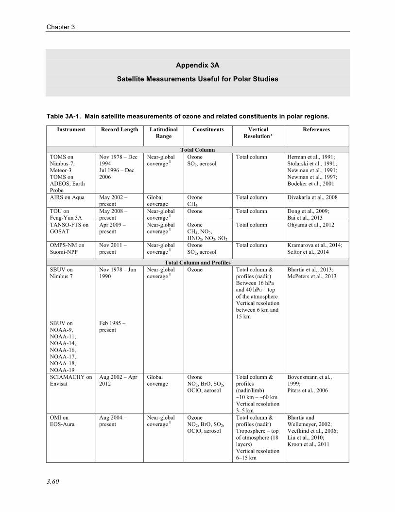
Chapter 3

 3.60

Appendix 3A

Satellite Measurements Useful for Polar Studies

Table 3A-1. Main satellite measurements of ozone and related constituents in polar regions.

Instrument Record Length Latitudinal Range

Constituents Vertical Resolution*

References

Total Column TOMS on Nimbus-7, Meteor-3 TOMS on ADEOS, Earth Probe

Nov 1978 – Dec 1994 Jul 1996 – Dec 2006

Near-global coverage 1

Ozone SO2, aerosol

Total column Herman et al., 1991; Stolarski et al., 1991; Newman et al., 1991; Newman et al., 1997; Bodeker et al., 2001

AIRS on Aqua May 2002 – present

Global coverage

Ozone CH4

Total column Divakarla et al., 2008

TOU on Feng-Yun 3A

May 2008 – present

Near-global coverage 1

Ozone

Total column Dong et al., 2009; Bai et al., 2013

TANSO-FTS on GOSAT

Apr 2009 – present

Near-global coverage 1

Ozone CH4, NO2, HNO3, NO2, SO2

Total column Ohyama et al., 2012

OMPS-NM on Suomi-NPP

Nov 2011 – present

Near-global coverage 1

Ozone SO2, aerosol

Total column Kramarova et al., 2014; Seftor et al., 2014

Total Column and Profiles SBUV on Nimbus 7 SBUV on NOAA-9, NOAA-11, NOAA-14, NOAA-16, NOAA-17, NOAA-18, NOAA-19

Nov 1978 – Jun 1990 Feb 1985 – present

Near-global coverage 1

Ozone Total column & profiles (nadir) Between 16 hPa and 40 hPa – top of the atmosphere Vertical resolution between 6 km and 15 km

Bhartia et al., 2013; McPeters et al., 2013

SCIAMACHY on Envisat

Aug 2002 – Apr 2012

Global coverage

Ozone NO2, BrO, SO2, OClO, aerosol

Total column & profiles (nadir/limb) ~10 km – ~60 km Vertical resolution 3–5 km

Bovensmann et al., 1999; Piters et al., 2006

OMI on EOS-Aura

Aug 2004 – present

Near-global coverage 1

Ozone NO2, BrO, SO2, OClO, aerosol

Total column & profiles (nadir) Troposphere – top of atmosphere (18 layers) Vertical resolution 6–15 km

Bhartia and Wellemeyer, 2002; Veefkind et al., 2006; Liu et al., 2010; Kroon et al., 2011

Polar Ozone

 3.61

TES on EOS-Aura

Aug 2004 – present

Global coverage

Ozone CH4, HNO3

Total column & profiles (nadir/limb) 0 km – 33 km Vertical resolution ~6–7 km

Beer, 2006; Bowman et al., 2006; Nassar et al., 2008

IASI on Metop-A IASI on Metop-B

Nov 2006 – present Nov 2012 – present

Global coverage

Ozone CH4, HNO3

Total column & profiles (nadir) Tropospheric layer – top of atmosphere Vertical resolution ~7 km

Coheur et al., 2005; Wespes et al., 2009; August et al., 2012

GOME-2 on Metop-A GOME-2 on Metop-B

Jan 2007 – present Dec 2012 – present

Near-global coverage 1

Ozone NO2, BrO, SO2, OClO, aerosol

Total column & profiles (nadir) Surface – top of atmosphere Vertical resolution ~7–15 km

van Roozendael et al., 2012; van Peet et al., 2014

OMPS-NP on Suomi-NPP

Nov 2011 – present

Near-global coverage 1

Ozone SO2, aerosol

Total column & profiles (nadir) Between 16 hPa and 40 hPa – top of the atmosphere Vertical resolution 6−15 km

Seftor et al., 2014

Profiles LIMS on Nimbus 7

Nov 1978 – May 1979

64°S – 84°N Ozone H2O, HNO3, NO2

Profiles (limb) Cloud top – ~0.01 hPa Vertical resolution ~3.7 km

Gille and Russell, 1984; Girard and Louisnard, 1984; Remsberg et al., 2007; Remsberg et al., 2010

SAM II on Nimbus 7

Nov 1978 – Dec 1993

64°S – 80°S and 64°N – 80°N

2 (coverage changed over the lifetime of the instrument)

PSCs, aerosol Profiles (solar occultation) Surface – ~160 km Vertical resolution ~0.5 km

Kent and McCormick, 1984; McCormick et al., 1981; McCormick and Trepte, 1986

SAGE I on AEM-B

Feb 1979 – Nov 1981

79°S – 79°N 2 Ozone NO2, aerosol

Profiles (solar occultation) Tropopause – ~55 km Vertical resolution 1 km

McCormick et al., 1984; Kent and McCormick, 1984; McCormick et al., 1989

SAGE II on ERBS

Oct 1984 – Jul 2005

80°S – 80°N 2 Ozone NO2, H2O, aerosol

Profiles (solar occultation) Tropopause – ~55 km Vertical resolution 1 km

Cunnold et al., 1989; McCormick et al., 1989; Damadeo et al., 2013

MLS on UARS Sep 1991 – Mar 2000

From 34° on one side of the equator to 80° on the other side – alternating every ~36 days

Ozone ClO, HNO3, H2O

Profiles (limb) 100 hPa – 0.22 hPa; Vertical resolution 3.5–5 km in the stratosphere, 5–8 km in the mesosphere

Barath et al., 1993; Waters et al., 1993; Livesey et al., 2003

Chapter 3

 3.62

CLAES on UARS

Oct 1991 – Apr 1993

From 34° on one side of the equator to 80° on the other –alternating every ~36 days

Ozone N2O, CFC-11, CFC-12, CH4, H2O, NO, NO2, HNO3, ClONO2, HCl, N2O5, PSCs, aerosol

Profiles (limb) 10 km – 60 km Vertical resolution ~2.5 km

Roche et al., 1993; Kumer et al., 1996; Massie et al., 1996

HALOE on UARS

Oct 1991 – Nov 2005

80°S – 80°N 2 Ozone NO2, H2O, NO, CH4, HCl, HF, PSCs, aerosol

Profiles (solar occultation) Cloud top – ~0.005 hPa Vertical resolution ~2.3 km

Russell et al., 1993; Schoeberl et al., 1995; Hervig et al., 1997

POAM II on SPOT-3

Sep 1993 – Nov 1996

55°N – 73°N, 63°S – 88°S 2

Ozone NO2, H2O, PSCs, aerosol

Profiles (solar occultation) ~5 km – ~60 km Vertical resolution ~1.5 km

Glaccum et al., 1996; Lumpe et al., 1997 ; Bevilacqua et al., 1997 ; Fromm et al., 2003

ILAS on ADEOS Oct 1996 – Jun 1997

57°N – 71°N, 64°S – 88°S 2

Ozone HNO3, NO2, N2O, CH4, H2O, PSCs, aerosol

Profiles (solar occultation) ~10 km – top of atmosphere Vertical resolution ~2 km

Sugita et al., 2002; Jucks et al., 2002; Nakajima et al., 2002; Yokota et al., 2002

POAM III on SPOT-4

Mar 1998 – Dec 2005

55°N – 73°N, 63°S – 88°S 2

Ozone NO2, H2O, PSCs, aerosol

Profiles (solar occultation) ~5km – ~60km Vertical resolution ~1.5 km

Lucke et al., 1999; Lumpe et al., 2002; Fromm et al., 2003

OSIRIS on Odin Nov 2001 – present

Near-global coverage 1

Ozone NO2, BrO, aerosol

Profiles (limb) Cloud tops – 55 km Vertical resolution 1.5 km in UTLS, 2 km higher up

Llewellyn et al., 2004; Brohede et al., 2007; McLinden et al., 2007

SMR on Odin Nov 2001 – present

~83°S – ~83°N

Ozone N2O, HNO3, H2O, ClO, NO, NOy

Profiles (limb) Vertical resolution 2.5–3.5 km

Urban et al., 2005; Barret et al., 2006

SAGE III on Meteor-3M 3

Feb 2002 – Dec 2005

50°S – 30°S, 50°N – 80°N

2

Ozone, NO2, H2O, OClO, aerosol

Profiles (solar occultation) Tropopause – ~55 km Vertical resolution 1 km

Wang et al., 2006

MIPAS on Envisat

Jun 2002 – Apr 2012

Global coverage

Ozone N2O, NO, NO2, HNO3, N2O5, ClONO2, CFCs, HOCl, ClO, H2O, H2O2, CH4, CO

Profiles (limb) ~8 km (20/40 km; middle/upper atmosphere mode) – 72 km (100 km; middle/upper atmosphere mode) Vertical resolution from ~2 km to ~8 km (depending on altitude)

Fischer et al., 2008; von Clarmann et al., 2009

GOMOS on Envisat

Aug 2002 – Apr 2012

Global coverage

Ozone NO2, H2O, PSCs, aerosol

Profiles (stellar occultation) ~15 km – ~100 km Vertical resolution 2–3 km

Kyrölä et al., 2004; Bertaux et al., 2010

Polar Ozone

 3.63

ILAS II on ADEOS II

Apr 2003 – Oct 2003

57°N – 71°N and 64°S – 88°S 2

Ozone HNO3, NO2, N2O, CH4, H2O, ClONO2, N2O5, CFC-11, CFC-12, PSCs, aerosol

Profiles (solar occultation) ~10 km – top of atmosphere Vertical resolution ~1.5 km

Sugita et al., 2006; Irie et al., 2006

ACE-MAESTRO on SCISAT

Feb 2004 – present

Near-global coverage 2

Ozone NO2, PSCs, aerosol

Profiles (solar occultation) 5 km – 35 km Vertical resolution ~1.2 km

McElroy et al., 2007; Nowlan et al., 2007

ACE-FTS on SCISAT

Feb 2004 – present

Near-global coverage 2

Ozone H2O, CH4, N2O, NO2, NO, NO3, HCl, HF, CO, CFC-11, CFC-12, N2O5, ClONO2, CH3Cl, SF6, H2O2, CCl4, HCFCs, ClO, HOCl

Profiles (solar occultation) ~5 km – 95 km Vertical resolution 3–4 km

Bernath et al., 2005; Boone et al., 2005; Jones et al., 2012

MLS on EOS-Aura

Aug 2004 – present

82°S – 82°N Ozone BrO, CH3Cl, ClO, CO, H2O, HCl, HNO3, HO2, OH, OCl, N2O, SO2

Profiles (limb) 215 hPa – 0.02 hPa Vertical resolution ~3 km in stratosphere, degrading to 4–6 km for pressures of 0.1 hPa or less

Waters et al., 2006; Livesey et al., 2006; Froidevaux et al., 2008; Santee et al., 2008

HIRDLS on EOS-Aura

Jan 2005 – Mar 2008

63°S – 80°N Ozone HNO3, CFC-11, CFC-12, NO2, N2O5, H2O, N2O, NO2, ClONO2, aerosol

Profiles (limb) 10 km – 55 km Vertical resolution ~1 km

Gille et al., 2008; Kinnison et al., 2008; Nardi et al., 2008

CALIOP on CALIPSO

Apr 2005 – present

82°S – 82°N PSCs, aerosol Profiles (nadir) Surface – 40km Vertical resolution 30–60 m

Winker et al., 2009; Pitts et al., 2009

OMPS-LP on Suomi-NPP

Nov 2011 – present

Near-global coverage 1

Ozone

Profiles (limb) 10 km – 60 km Vertical resolution 2 km

Rault and Loughman, 2013

* Vertical resolution only applies to ozone. 1 Apart from polar night latitudes. 2 Because of their particular viewing geometry and measurement technique, solar occultation instruments do not provide global

coverage on a daily basis. 3 A replica of the SAGE III Meteor-3M instrument is scheduled to be deployed on the International Space Station (ISS) in 2015.

Although SAGE-III/ISS will measure ozone, water vapor, and a few other atmospheric constituents (NO2, NO3, and OClO, as well as aerosols and clouds), its coverage will be focused on middle and low latitudes.