Upstream competitionand buyer mergersand buyer mergers

Stéphane CapriceToulouse School of Economics

GREMAQ-INRAGREMAQ INRA

1

Buyer firms often merge in order to obtain lower prices from suppliersobtain lower prices from suppliers

What is the contribution of this paper?Explain in which circonstances merging buyers may obtain lowermerging buyers may obtain lower prices in negotiation with suppliers

2

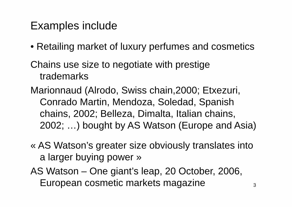
Examples include

• Retailing market of luxury perfumes and cosmetics

Chains use size to negotiate with prestige trademarks

Marionnaud (Alrodo, Swiss chain,2000; Etxezuri, Conrado Martin Mendoza Soledad SpanishConrado Martin, Mendoza, Soledad, Spanish chains, 2002; Belleza, Dimalta, Italian chains, 2002; ) bought by AS Watson (Europe and Asia)2002; …) bought by AS Watson (Europe and Asia)

« AS Watson’s greater size obviously translates into g ya larger buying power »

AS Watson – One giant’s leap, 20 October, 2006,3

AS Watson One giant s leap, 20 October, 2006, European cosmetic markets magazine

• Home improvement retail sector

Kingfisher currently expanding in 11 European and Asian marketsAsian markets

Size enables it to negotiate better with big i t ti l liinternational suppliers

• Grocery retail market Grocery retail market

European cross-border buying alliancesEMD, AMS, Intercoop/NAF INT, Eurogroup, SED,

Europartners, BIGSp ,Around two-fifths of the total EU market

4

SchemaA B A B

1 2 1 2

Size matters

Merging buyers continue to buy from both sellersA d b di ti

5And buyer merger causes no disruption

Related literature

Chipty and Snyder, 1999 (RES)Raskovich, 2003 (JIE)

6

A simple Framework: the bargainingA simple Framework: the bargaining interface model with a monopoly supplier

A ( ) ( )

h

i ii

T x C X

X

−∑

∑where ii

X x=∑

( )

1 2 ( ) N

(…)

( ) ( )1 1 1R x T x−

1 2 (…) N

( ) ( )N N NR x T x−( ) ( )1 1 1

N i d d l k

( ) ( )2 2 2R x T x−( ) ( )N N N

7N independent outlets or markets

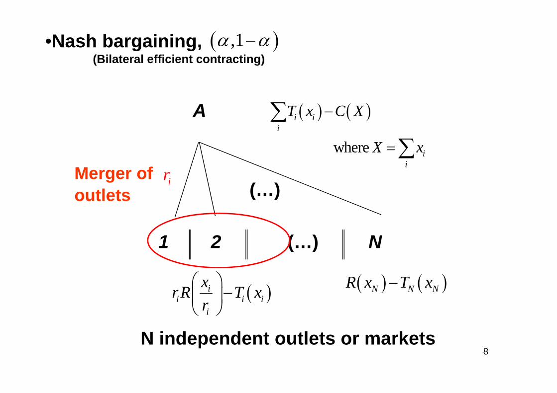
( ),1α α−•Nash bargaining,(Bilateral efficient contracting)

( ) ( )T C X∑A

(Bilateral efficient contracting)

( ) ( )

where

i ii

i

T x C X

X x

−

=

∑

∑

A

where ii

X x∑ir (…)

Merger ofoutlets

1 2 ( ) N

( )outlets

( )ix⎛ ⎞ ( ) ( )N N NR x T x−

1 2 (…) N

( )ii i i

i

xrR T xr

⎛ ⎞−⎜ ⎟

⎝ ⎠

( ) ( )N N NR x T x

8N independent outlets or markets

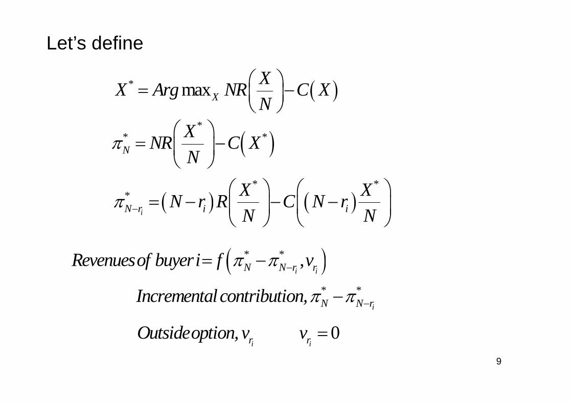
Let’s define

( )* maxXXX Arg NR C XN

⎛ ⎞= −⎜ ⎟⎝ ⎠⎝ ⎠

( )*

* *N

XNR C XN

π⎛ ⎞

= −⎜ ⎟⎝ ⎠

( )N⎝ ⎠

( ) ( )* *

* X XN r R C N rπ⎛ ⎞ ⎛ ⎞

= − − −⎜ ⎟ ⎜ ⎟( ) ( )iN r i iN r R C N r

N Nπ − = − − −⎜ ⎟ ⎜ ⎟

⎝ ⎠ ⎝ ⎠

( )* * ,i iN N r rRevenuesof buyeri f vπ π −= −

* *Incrementalcontribution π πiN N rIncrementalcontribution,π π −−

0r rOutsideoption, v v =9

i ir rp ,

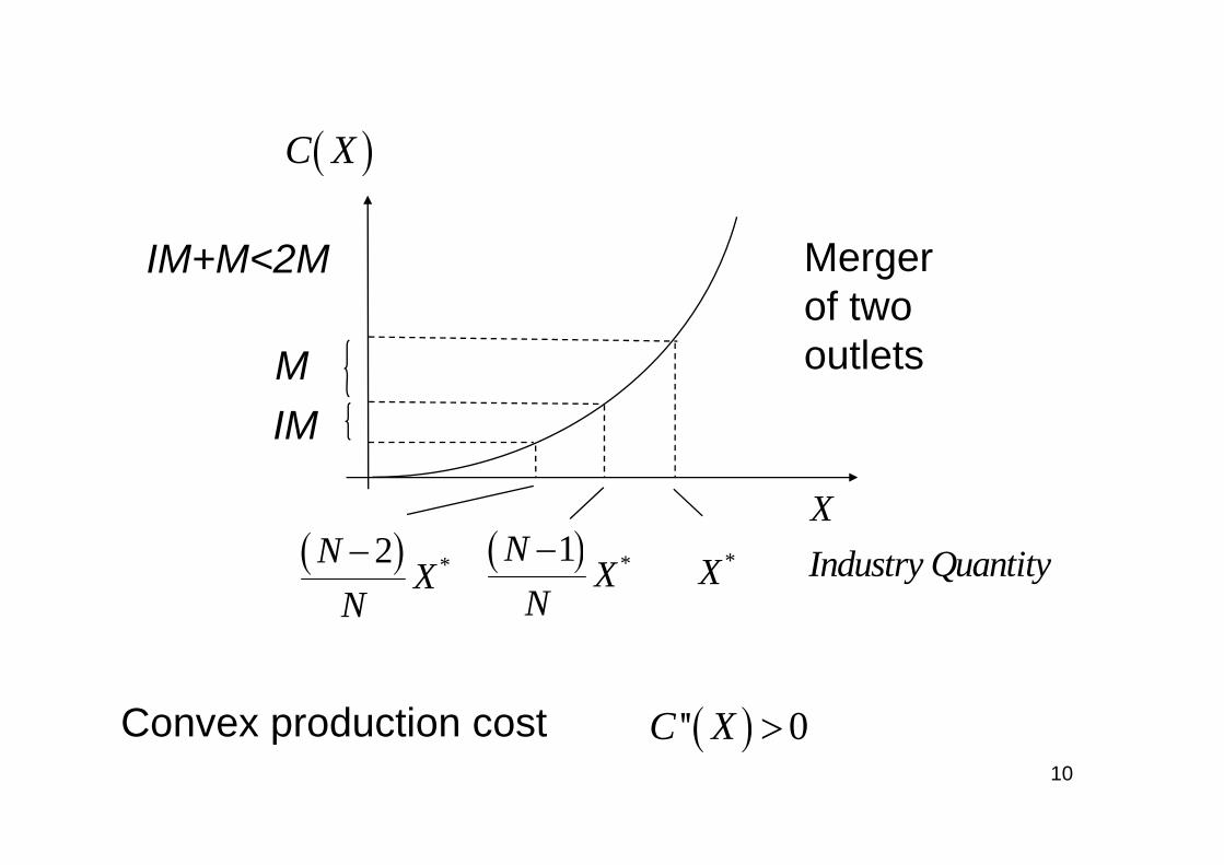
( )C X( )C X

IM+M<2M Mergerof two

IMM outlets

X( )

IM

Industry Quantity*X( ) *1NX

N−( ) *2N

XN−

Convex production cost ( )'' 0C X >10

Convex production cost ( ) 0C X >

*π

MMergerof two

xπ

IMM of two

outlets

IM+M>2M

xN1N −2N −Outlets

Industry Surplus *xπ

11

* *iN N rπ π −−

ir21Number of outletscontrolled by a buyer i

21

Incremental contribution * *iN N rπ π −−

y y

12

i

• The merging of buyers account for a larger fraction of the supplier’s total sales andfraction of the supplier s total sales and thus negotiate less well at the margin

• Supplier’s increasing marginal productionSupplier s increasing marginal production costs (concave industry surplus)

i t l t dincremental cost decreases more steeply than in proportion with buyer size

large buyers pay a lower price per unit

13

• Our frameworkWhat is new?Upstream competition to supply imperfect

substitutessubstitutes

• Focus on buyer powerDirect bargaining effect (1)Direct bargaining effect (1)

See the model with a monopoly supplierIndirect bargaining effect (2)

Related to increasing the buyer’s outside option14

g y p

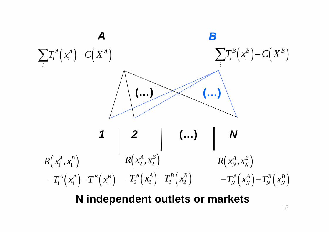
A BA

( ) ( )A A Ai iT x C X−∑

B( ) ( )B B B

i ii

T x C X−∑i

( ) ( )

i

(…) (…)

1 2 (…) N

( )1 1,A BR x x ( )2 2,A BR x x ( ),A BN NR x x

N i d d t tl t k t( ) ( )1 1 1 1

A A B BT x T x− − ( ) ( )2 2 2 2A A B BT x T x− − ( ) ( )A A B B

N N N NT x T x− −

15N independent outlets or markets

A BA

( ) ( )A A Ai iT x C X−∑

B( ) ( )B B B

i ii

T x C X−∑i

( ) ( )

i

M f (…) (…)Merger ofoutlets

ir

1 2 (…) N

( ) ( )A B

A A B Bi ix xrR T x T x⎛ ⎞⎜ ⎟

( ),A BN NR x x

( ) ( ),i i i i ii i

rR T x T xr r

− −⎜ ⎟⎝ ⎠ ( ) ( )A A B B

N N N NT x T x− −

16N independent outlets or markets

The bargaining protocolA simple Framework:Bilateral negotiations sufficiently complex to rule g y pout problems of double marginalization

Bil t l ffi i t t ti• Bilateral efficient contracting, At equilibrium, bilateral supplies maximize total

industry profits.• Off equilibrium,qIf bargaining breaks down between one buyer and

one supplier k, we allow for renegotiation betweenone supplier k, we allow for renegotiation between the buyer and the other supplier -k.

( ),1α α−17

( )

Let’s define

( ) ( ),* ,*, arg max ,A B

A BA B A B

A BX X

X XX X NR C X C XN N

⎛ ⎞= − −⎜ ⎟

⎝ ⎠( ) ( ), A BX X N N⎜ ⎟

⎝ ⎠Bilateral efficient contracting, At ilib i bil t l li i i t t l i d tAt equilibrium, bilateral supplies maximize total industry

profits.

( ) ,*arg max 0,ki

k k k kii i i k ix

N rx r R x C X xN−

− − − −−

−⎛ ⎞= − +⎜ ⎟⎝ ⎠

%N⎝ ⎠

Following a breakdown between one buyer and the li ksupplier k

Off equilibrium, renegotiation between the buyer and the other li th li k

18supplier, the supplier -k.

* *A B⎛ ⎞ ( ) ( ),* ,*

* ,* ,*,A B

A BN A B

X XNR C X C XN N

π⎛ ⎞

= − −⎜ ⎟⎝ ⎠

( ),* ,* ,*

,* , 0,A B k

kN r i i

X X XN r R r Rπ−⎛ ⎞ ⎛ ⎞

= − +⎜ ⎟ ⎜ ⎟( )

( ) ( ),*

,*

, ,iN r i i

kk

N N N

XC N C X

−

−

⎜ ⎟ ⎜ ⎟⎝ ⎠ ⎝ ⎠⎛ ⎞⎜ ⎟( ) ( ),k

k i kC N r C XN −− − −⎜ ⎟

⎝ ⎠* * kA B ⎛ ⎞⎛ ⎞ %( ),* ,*

,~ , 0,i

kA Bk iN r i i

i

xX XN r R r RN N r

π−

−

⎛ ⎞⎛ ⎞= − + ⎜ ⎟⎜ ⎟

⎝ ⎠ ⎝ ⎠

%

( ) ( ),* ,*k k

kk i k i i

X XC N r C N r xN N

−−

−

⎛ ⎞ ⎛ ⎞− − − − +⎜ ⎟ ⎜ ⎟

⎝ ⎠ ⎝ ⎠%

19

⎝ ⎠ ⎝ ⎠

Revenuesof buyeri ( )( )* ,* ,~ ,*,i i i i

k k kN N r r N r N r

Revenuesof buyerif v

in negotiation with kπ π π π− − −= − −

* ,*kN NIncrementalcontribution, π π−

iN N rIncrementalcontribution, π π −

( ),~ ,*k kOutsideoption v π π−( )i i ir N r N rOutsideoption, v π π− −

20

For an illustration,

Consider the bargaining game of the merging buyers(merger of two outlets) with respect to supplier A

Suppliers A and B, convex production costs2 * ,*kπ π⎡ ⎤∂ ⎣ ⎦

Di t b i i ff t (+)2 0iN N r

irπ π −⎡ ⎤∂ −⎣ ⎦ >∂

Direct bargaining effect: (+),~ ,*k k

N Nπ π⎡ ⎤∂ −⎣ ⎦2 0i iN r N r

irπ π− −⎡ ⎤∂⎣ ⎦ <

∂I di t b i i ff t ( )

21Indirect bargaining effect: (-)

( )AC X

( )'' 0AC XIM M 2M

( )AAC X

( )'' 0AAC X >IM+M<2M

IMM

AX( )1N( )2N −

IM

Industry Quantity,*AX( ) ,*1 AN

XN−( ) ,*2 AN

XN

22

* ,*i

AN N rπ π −−

irb f l21 Number of outlets

controlled by a buyer i

21

Incremental contribution * ,*i

AN N rπ π −−

23Direct bargaining effect: (+)

( )BC X( )BC X

( )'' 0BBC X >IM

M

IM+M>2M BXIndustry Quantity

,*BX ( ) ,*1

1 B BNX x

N−

+ % ( ) ,*1 2

2 B BNX x

N +

−+ %

N N

24

,~ ,*k kN Nπ π−

i iN r N rπ π− −

irNumber of outlets1 2 Number of outletscontrolled by a buyer i

( )*k kOutside option ( ),~ ,*i i i

k kr N r N rv π π− −−

25Indirect bargaining effect: (-)

More generally,

Average profit by outlet of buyer i:

,* ,*,* ,* A BA Bi it tX XRφ

⎛ ⎞= ⎜ ⎟,i

i i

RN N r r

φ = − −⎜ ⎟⎝ ⎠

Size discountSize discount whenever:

,* ,*1 k kt tφ ⎡ ⎤∂ ∂, ,

,

1 0k k

i i i

k A Bi i i i

t tr r r rφ

=

⎡ ⎤∂ ∂= − >⎢ ⎥∂ ∂⎣ ⎦

∑

⇔ 0k ki i

k A BDE IE

=

+ >∑26

,k A B=

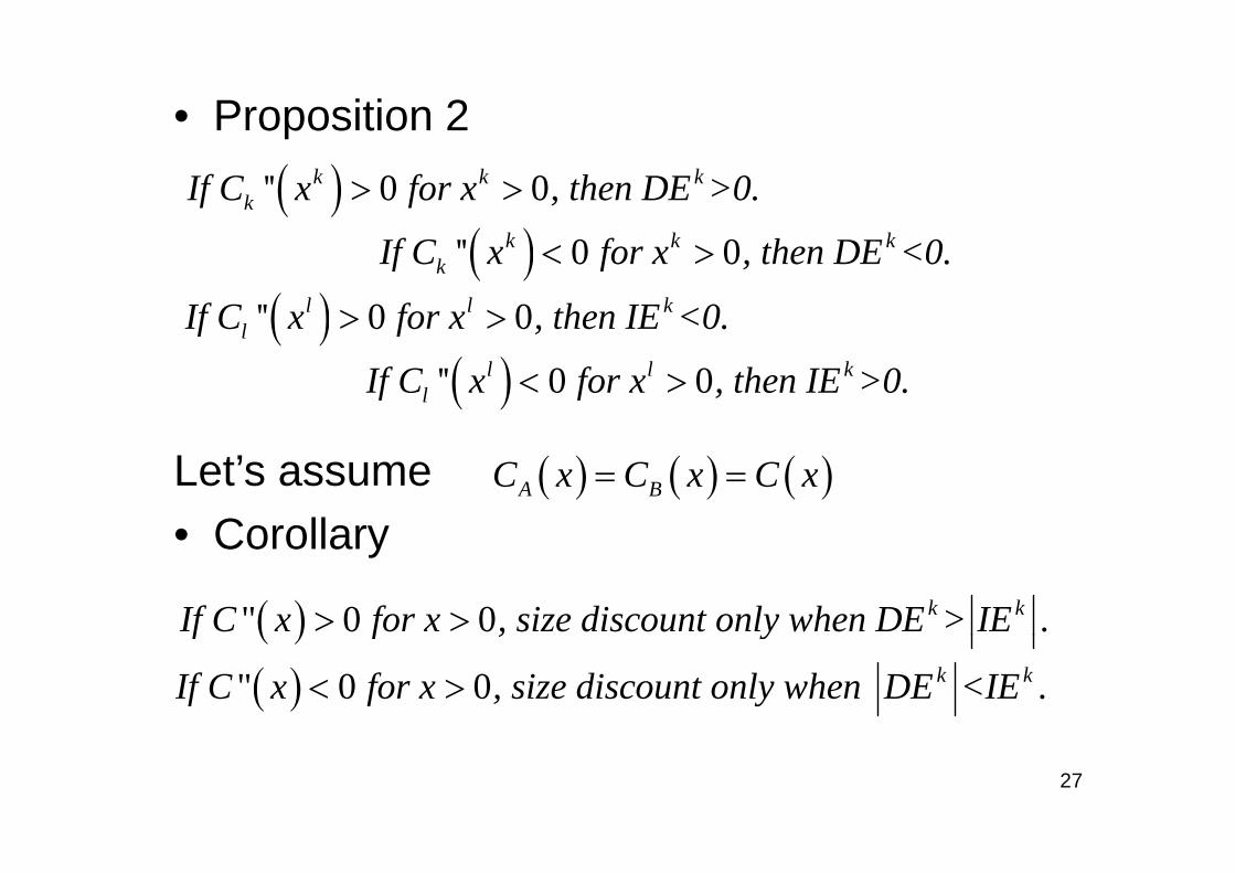
• Proposition 2

( )'' 0 0k k kkIf C x for x , then DE >0.> >

( )k k kf f h( )'' 0 0k k kkIf C x for x , then DE <0.< >

( )'' 0 0l l klIf C x for x , then IE <0.> >( )l

( )'' 0 0l l klIf C x for x , then IE >0.< >

Let’s assume • Corollary

( ) ( ) ( )A BC x C x C x= =

• Corollary

( )" 0 0 k kIf C x for x , size discount only when DE > IE .> >( )f f , y

( )" 0 0 k kIf C x for x , size discount only when DE <IE .< >

27

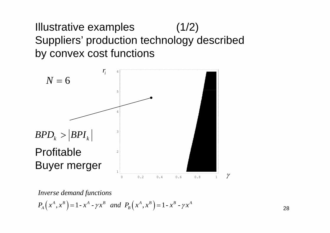
Illustrative examples (1/2)S li ’ d ti t h l d ib dSuppliers’ production technology describedby convex cost functions

6N =6ir

4

5

k kBPD BPI> 3

2ProfitableBuyer merger

0 0.2 0.4 0.6 0.8 1

1

Inverse demand functions

γy g

28( ) ( ), 1- - , 1- -A B A B A B B AA B

f

P x x x x and P x x x xγ γ= =

In the first example, any increase in upstreamcompetitiveness impairs the level of mergingbuyers’ outside option, increasing the relative importance of the negative indirect bargainingeffect.

29

Illustrative examples (2/2)Suppliers’ production technology describedSuppliers production technology describedby concave cost functions

5

6

BPD BPI<6N =

ir

4

5k kBPD BPI<

Profitable3

ProfitableBuyer merger

0 0 2 0 4 0 6 0 8 1

1

2

0 0.2 0.4 0.6 0.8 1

Inverse demand functions

γ

30( ) ( ), 1- - , 1- -A B A B A B B AA B

f

P x x x x and P x x x xγ γ= =

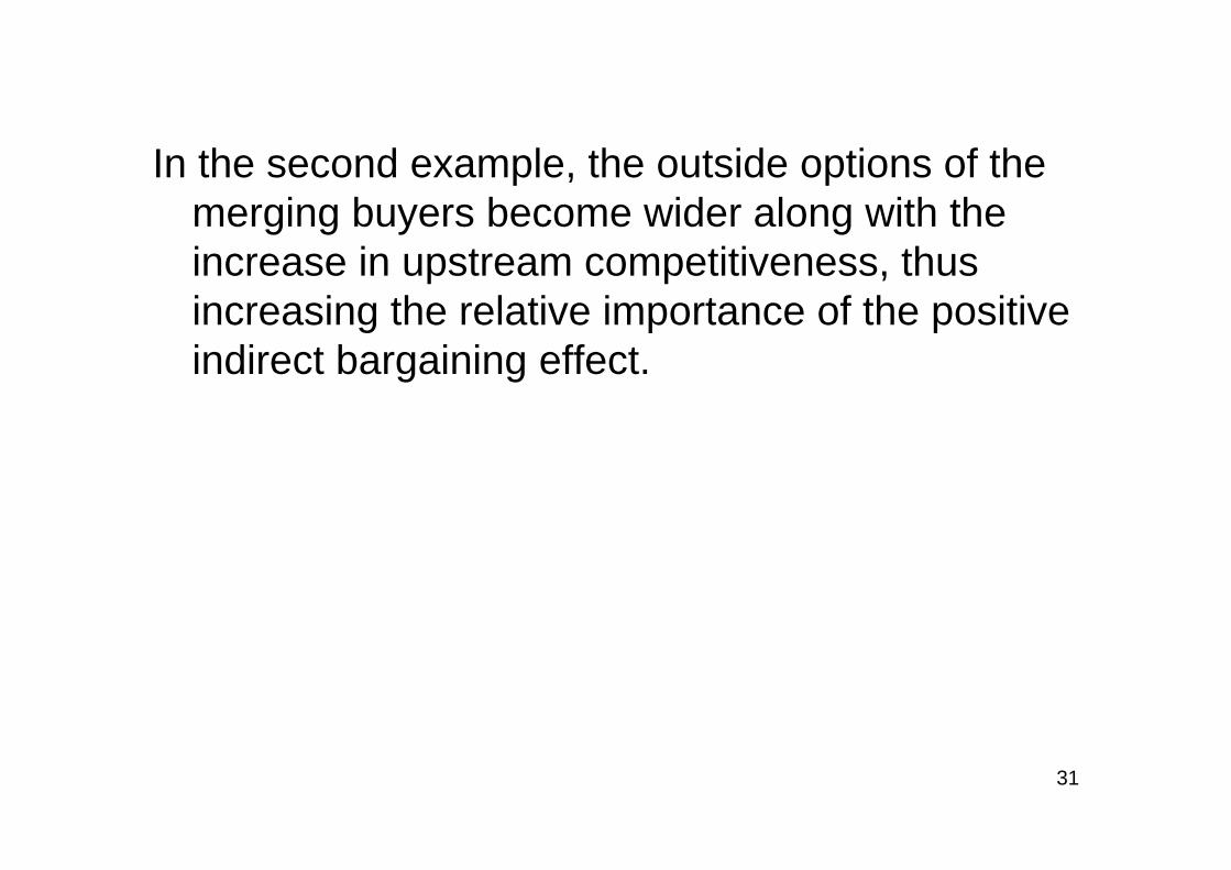
In the second example, the outside options of the merging buyers become wider along with the increase in upstream competitiveness, thus increasing the relative importance of the positive indirect bargaining effect.

31

Concluding remarks

• Focus on buyer power, two sourcesDirect bargaining effect (1)Direct bargaining effect (1) Indirect bargaining effect (2) (Related to increasing the buyer’s outside option)

• Chipty and Snyder (1999) concludes in the cable-television industry that merger should worsen than y genhance the buyers’ bargaining position since the upstream production cost function was concave.

New insight since buyer merger now may beprofitable even if production cost functions are concave

32

profitable even if production cost functions are concave.

• Bilateral efficient contracting, equilibrium quantities are unchanged in buyer mergers.Dobson and Waterson (1997)≠

• The framework can be used to analyze the potential adverse long term consequences ofpotential adverse long-term consequences of buyer power on suppliers’ economic viability and their incentives to invest and innovatetheir incentives to invest and innovate

Inderst and Wey (2003, 2006), Inderst and Shaffer (2006)

33

• Dana (2007); Inderst and Shaffer (2007)Wh b i fi it t b≠

Where buyer group or merging firms commit to buy exclusively from a single seller.

• Inderst (2006), Smith and Thanassoulis (2006)≠Imperfect substitutes (More general insight, concave

costs, …), )

34