upwind 1a2 metrology. final report - dtu orbitorbit.dtu.dk/files/5615242/upwind 1a2...
TRANSCRIPT

General rights Copyright and moral rights for the publications made accessible in the public portal are retained by the authors and/or other copyright owners and it is a condition of accessing publications that users recognise and abide by the legal requirements associated with these rights.
• Users may download and print one copy of any publication from the public portal for the purpose of private study or research. • You may not further distribute the material or use it for any profit-making activity or commercial gain • You may freely distribute the URL identifying the publication in the public portal
If you believe that this document breaches copyright please contact us providing details, and we will remove access to the work immediately and investigate your claim.
Downloaded from orbit.dtu.dk on: Jun 04, 2018
UPWIND 1A2 Metrology. Final Report
Eecen, P.J.; Wagenaar, J.W.; Stefanatos, N.; Friis Pedersen, Troels; Wagner, Rozenn; Hansen, KurtSchaldemose
Publication date:2011
Document VersionPublisher's PDF, also known as Version of record
Link back to DTU Orbit
Citation (APA):Eecen, P. J., Wagenaar, J. W., Stefanatos, N., Friis Pedersen, T., Wagner, R., & Hansen, K. S. (2011). UPWIND1A2 Metrology. Final Report. Energy Research Centre of the Netherlands (ECN). (ECN-E-11-013).

FINAL REPORT UPWIND 1A2 METROLOGY
P.J. Eecen, J.W. Wagenaar (ECN)
N. Stefanatos (CRES)
T.F. Pedersen, R. Wagner (Riso-DTU)
K.S. Hansen (DTU-MEK)
ECN-E--11-013 FEBRUARI 2011

2 Confidential ECN-E--11-013
Acknowledgement/Preface The work described in this report is carried out within the framework of the European UPWIND research project under contract with the European Commission. CE Contract Number: 019945 (SES6) ECN Project number: 7.9466 Abstract The UpWind project is a European research project that focuses on the necessary up-scaling of wind energy in 2020. Among the problems that hinder the development of wind energy are measurement problems. For example: to experimentally confirm a theoretical improvement in energy production of a few percent of a new design by field experiments is very hard to almost impossible. As long as convincing field tests have not confirmed the actual improvement, the industry will not invest much to change the turbine design. This is an example that clarifies why the development of wind energy is hindered by metrology problems (measurement problems). Other examples are in the fields of:
• Warranty performance measurements • Improvement of aerodynamic codes • Assessment of wind resources
In general terms the uncertainties of the testing techniques and methods are typically much higher than the requirements. Since this problem covers many areas of wind energy, the work package is defined as a crosscutting activity. The objectives of the metrology work package are to develop metrology tools in wind energy to significantly enhance the quality of measurement and testing techniques. The first deliverable was to perform a state of the art assessment to identify all relevant measurands. The required accuracies and required sampling frequencies have been identified from the perspective of the users of the data (the other work packages in UpWind). This work led to the definition of the Metrology Database, which is a valuable tool for the further assessment and interest has been shown from other work packages, such as Training. This report describes the activities that have been carried out in the Work Package 1A2 Metrol-ogy of the UpWind project. Activities from Risø are described in a separate report: T.F. Peder-sen and R. Wagner, ‘Advancements in Wind Energy Metrology UPWIND 1A2.3’, Risø-R-1752.

ECN-E--11-013 Confidential 3
Contents
1. Introduction 7 1.1 Work Package 1A2 Metrology 8 1.2 References 8
2. Deliverable D 1A2.1: List of Measurement Parameters 9 2.1 Other areas of investigation 11
2.1.1 Air Foil data 11 2.1.2 Traceability in measurements 12
2.2 Integration with other work packages in UpWind 13 2.3 Discussion and Conclusions 19 2.4 References 19
3. The Metrology Database 21 3.1 Introduction 21 3.2 Database structure 21 3.3 Access to the database 23 3.4 Discussion and Conclusions 25 3.5 References 25
4. Turbulence normalization combined with the equivalent wind speed method 27 4.1 Introduction 27 4.2 Effect of the turbulence intensity 27 4.3 Equivalent wind speed and turbulence 28 4.4 Description of Albers' method 28 4.5 Combination with the equivalent wind speed 29 4.6 Conclusions 30 4.7 References 30
5. Improvements in power performance measurement techniques 31 5.1 EWTW and Data taking 31
5.1.1 Site description 31 5.1.2 IEC Standards and data selection 32
5.2 Atmospheric conditions 34 5.2.1 Air density 34 5.2.2 Stability 35 5.2.3 Turbulence 38 5.2.4 Vertical wind shear 40 5.2.5 Cross correlations 44
5.3 Power Curve Corrections 46 5.3.1 Air density 46 5.3.2 Turbulence 47 5.3.3 Vertical wind shear: Wind speed corrections 49 5.3.4 Vertical wind shear: Power corrections 53
5.4 Conclusions 57 5.5 References 58
6. Power performance measurement 59 6.1 Influence of shear - Introduction 59 6.2 Shear and turbine aerodynamics 59 6.3 Equivalent wind speed 60 6.4 Experimental validation of the method 61 6.5 Conclusions 62 6.6 References 62
7. Influence of offshore wakes on power performance at large distances 63

4 Confidential ECN-E--11-013
7.1 Introduction 63 7.2 Data selection 64 7.3 Null measurements 64 7.4 Single Wakes 65
7.4.1 Turbulence intensity: Wind speed dependency 65 7.4.2 Added turbulence 66
7.5 Multiple wakes 69 7.6 Conclusions 72 7.7 References 72
8. Guideline to wind farm wake analysis 73 8.1 Introduction 73
8.1.1 Purpose 73 8.1.2 Signals 73 8.1.3 Definitions 74
8.2 Data preparation 75 8.3 Signals, organization and synchronization 75
8.3.1 Wind farm layout 76 8.3.2 Data qualification 78 8.3.3 Derived parameters 80 8.3.4 Identifications of descriptors and flow cases 82 8.3.5 Data filtering 84
8.4 Data query and wake analysis 85 8.5 Conclusion 90 8.6 Acknowledgement 90 8.7 References 90
9. Recommendation to IEC61400-12-2 Wake sector analysis 91 9.1 Introduction and background 91
9.1.1 Additional analysis turbulence dependency 94
10. Classification of atmospheric stability for offshore wind farms 95 10.1 Introduction 95
10.1.1 Instrumentation 95 10.2 Determination of atmospheric stability. 97
10.2.1 Gradient method. 97 10.2.2 Sonic measurements 98 10.2.3 Bulk-Richardson number 99
10.3 Site classification 103 10.3.1 Turbulence intensity correlated to atmospheric stability. 104
10.4 Wake analysis 105 10.4.1 Power deficits for 7D spacing. 105 10.4.2 Power deficit for 9.4D spacing. 106 10.4.3 Power deficit for 10.4D spacing. 107
10.5 Conclusion 107 10.6 Acknowledgement 107 10.7 References 108
11. Quantification of Linear Torque Characteristics of Cup Anemometers with Step Responses 109 11.1 Introduction 109 11.2 Basic torque characteristics of cup anemometers 109 11.3 Linearized torque characteristics of a typical cup anemometer 110 11.4 Classification of cup anemometers with linear torque 110 11.5 Step response measurement procedures 111 11.6 Step response measurements – an example 112 11.7 Conclusions 114

ECN-E--11-013 Confidential 5
11.8 References 114
12. Generics of nacelle anemometry 115 12.1 Introduction 115 12.2 Review of nacelle anemometry 115 12.3 Specific background 115 12.4 Flow induction at rotor 116
12.4.1 Betz and nacelle anemometry 116 12.5 Conclusions 120 12.6 References 121
13. Spinner anemometry as an alternative to nacelle anemometry 123 13.1 Introduction 123 13.2 Wind measurement in front of the rotor 123 13.3 Free field comparison to 3D sonic anemometer 125 13.4 Calibration of the spinner anemometer 126 13.5 Tests of spinner anemometers on wind turbines 126 13.6 Conclusions 127 13.7 References 127
14. Long term stability of cup anemometer operational characteristics 129 14.1 Identification of the problem 129 14.2 Method of approach 129
14.2.1 Results 130 14.2.2 Discussion 131
14.3 Applicability of current power performance measurement recommended practices in various types of terrains. 132 14.3.1 Identification of the problem 132 14.3.2 Method of approach 132 14.3.3 Results and discussion 132
14.4 Definition of reference wind speed for power curve measurements of large wind turbines (>2.0 MW). 133 14.4.1 Identification of the problem 133 14.4.2 Method of approach 133 14.4.3 Results and discussion 134
14.5 Actions taken – improvements –response of wind energy community: 136 14.6 References 136
Appendix A Aerodynamics & Aero-elastics, Rotor structures Materials, and Turbine Foundations 137
Appendix B Control systems and Condition Monitoring 140
Appendix C Transmission and conversion and Electrical Grid 143
Appendix D Flow and Remote Sensing 145
Appendix E Power Performance analysis (IEC 61400-12-1) 146
Appendix F Noise Measurements (IEC 61400-11) 147

6 Confidential ECN-E--11-013

ECN-E--11-013 Confidential 7
1. Introduction
The UpWind project UpWind is a European project funded under the EU's Sixth Framework Programme (FP6). The project looks towards the wind power of tomorrow, more precisely towards the design of very large wind turbines (8-10MW), both onshore and offshore. Furthermore, the research also fo-cuses on the requirements to the wind energy technology of 20MW wind turbines. The challenges inherent to the creation of wind farms of several hundred MW request the high-est possible standards in design, complete understanding of external design conditions, the de-sign of materials with extreme strength to mass ratios and advanced control and measuring sys-tems geared towards the highest degree of reliability, and critically, reduced overall turbine mass. The wind turbines of the future necessitate the re-evaluation of the turbine itself for its re-conception to cope with future challenges. The aim of the project is to develop accurate, verified tools and component concepts that the industry needs to design and manufacture this new type of turbine. UpWind focuses on design tools for the complete range of turbine components. It addresses the aerodynamic, aero-elastic, structural and material design of rotors. Critical analy-ses of drive train components will be carried out in the search for breakthrough solutions. The UpWind consortium, composed of over 40 partners, brings together the most advanced Euro-pean specialists of the wind industry. Expected results In the UpWind project research will lead to accurate, verified tools and some essential compo-nent concepts the industry needs to design and manufacture the new breed of very large wind turbines. Among others, UpWind will address the aerodynamic, aero-elastic, structural and ma-terial design aspects of rotors. Future wind turbine rotors may have diameters of over 150 me-ters. These dimensions are such that the flow in the rotor plane is non-uniform as a result of which the inflow may vary considerably over the rotor blade. Full blade pitch control would no longer be sufficient. That is why UpWind will investigate local flow control along the blades, for instance by varying the local profile shape. New control strategies and new control elements must be developed and critical analyses of drive train components must be carried out in the search for breakthrough solutions. Furthermore, wind turbines are highly non-linear, reactive machines operating under stochastic external conditions. Extreme conditions may have an impact a thousand times more demanding on, for instance, the mechanical loading than average conditions require. Understanding pro-foundly these external conditions is of the utmost importance in the design of a wind turbine structure with safety margins as small as possible in order to realise maximum cost reductions. A similar argument applies to the response of the structure to external excitations. In order to make significant progress in this field, more accurate, linearly responding measuring sensors and associated software are needed. Preferably, the sensors should remain stable and accurate during a considerable part of the operational lifetime of a wind turbine. UpWind will explore measuring methods and will look more in detail into new remote sensing techniques for measur-ing wind velocities. The validation and verification of the analyses, tools and techniques depend on reliable and appropriate measurements. The task of the work package ‘Metrology’ is to iden-tify the critical issues in measurement techniques and to find solutions for the most critical ones. More information on the UpWind project is found on the website: www.upwind.eu

8 Confidential ECN-E--11-013
1.1 Work Package 1A2 Metrology As the project includes many scientific disciplines which need to be integrated in order to arrive at specific design methods, new materials, components and concepts, the project's organisation structure is based on work packages which variously deal with scientific research, the integra-tion of scientific results, and their integration into technical solutions. Since the measurement problems are related to several areas in the wind energy, the work package Metrology is defined as an integrating work package. The metrology problems to develop wind turbine technology are the focus of this work package since the development of wind energy is hindered by measurement problems. In particular the fluctuating wind speed introduces large uncertainties and these fluctuations in the wind are ex-perienced throughout the entire wind turbine. An example of a problem through measurement uncertainties is that it is almost impossible to confirm anticipated small performance improve-ments resulting from design modifications by means of field tests. As long as convincing field tests have not confirmed the actual improvement, the industry will be hesitant in investing in turbine design improvements. Furthermore, the developments within the UpWind project will require validation that is based on reliable and appropriate measurements. The objective of the metrology work package is to develop metrology tools in wind energy to significantly enhance the quality of measurement and testing techniques. The first deliverable has been published being the first step to reach this objective and the list of parameters that should be measured in wind energy. The list has been developed in close collaboration with the other UpWind project work packages. The second deliverable is to find theoretical solutions for the identified metrology problems. Based on the deliverable 1 [1], the list of measurement prob-lems, it has been analysed what the precise consequences of the identified problems are and in which directions possible solutions can be found. This has been reported [2] and a database structure has been designed to make the detailed information available to the other work pack-ages.
1.2 References [1] P.J. Eecen, N. Stafanatos, S.M. Petersen, K.S. Hansen, UpWind METROLOGY Deliv-
erable D1A2.1: List of Measurement Parameters, ECN-E--07-015 [2] P.J. Eecen, N. Stefanatos, T.F. Pedersen, K.S. Hansen, UpWind METROLOGY. Deliv-
erable D 1A2.2; Metrology Database - Definition ECN-E--08-079

ECN-E--11-013 Confidential 9
2. Deliverable D 1A2.1: List of Measurement Parameters
The development of metrology tools to significantly enhance the quality of measurement and testing techniques in wind energy is carried out in three steps. These steps are described in the work programme and are defined as deliverables. The three steps (deliverables) are
1. Problem identification: determination of the parameters that must be measured for the various problems encountered in wind energy and the required accuracies.
2. Available techniques and theoretical solutions: for the identified parameters the state-of-the-art measurement techniques are described, the problems that may be encountered are described and possible theoretical solutions are presented.
3. The practical value of the proposed solutions is demonstrated. After finishing the second step where the theoretical solutions are presented, a work programme for the demonstration phase is defined. This report presents lists of parameters that should be measured for the various subjects in wind energy. Since the work packages in the UpWind project are divided along these subjects, the lists are specified for the different work packages. The lists have the intention not only to in-clude the present-day techniques, but rather describe required or desired measurement tech-niques for the future 20MW wind turbines. The list has been made after interaction with the work packages in the UpWind project. All members of these work packages did have the oppor-tunity to comment on the list or add further required measurements. When setting up the lists of parameters, it was found that the most valuable list limits itself to the following columns
Parameter / Signal Unit Desired
accuracy Traceable
(Y/N) Sampling frequency
range [Hz] Required / Optional
Measurement position
Where the columns are:
• Parameter / Signal: The name of the parameter or signal that must be measured. • Unit: The unit in which the parameter should be measured. • Desired accuracy: The desired accuracy with which the parameter should be deter-
mined for the specific task. This means that a single parameter could have quite differ-ent requirements for the different applications (work packages).
• Traceability: Whether or not the parameter should have a traceable value. In general all values that are measured should be traceable, otherwise you will have a 'floating' value. Although almost all values should be traceable, it is still included in the list to remind the experimenters and users of experimental data of the importance of traceability. Fur-ther information on traceability is presented in section 2.1.2.
• Sampling frequency range: The required frequency range for the specific purpose. For many parameters a minimum sampling frequency is provided. For some of the more general parameters, the reader is reminded that the sampling frequency should be eight times larger than the highest frequency to be studied.
• Required or Optional: indicate whether the parameter is required for the purpose or can be optional. Optional is also indicated when we expect that it will be required for future techniques but at the moment it is (only) optional. It must be noted that in many cases the optional measurements can improve the final accuracy and reliability of the measurements.
• Measurement position: the location where the parameter should be measured.

10 Confidential ECN-E--11-013
There are some remarks: 1. Measurands could be used for various applications. For the different applications, usually
there are different requirements with respect to accuracy, sampling frequency or reliability. 2. For each measurand is indicated whether or not it is required. One should keep in mind that
what is optional today might be required in the future because of for example advance-ments in turbine control or measurement techniques.
3. The measurement position does not include the mounting, since this is specific for each in-strument and measurement technique. The mounting will be included in the list of meas-urement devices (deliverable D 1A2.2). In the list presented in this report is indicted the lo-cation in the turbine, or around the turbine where the measurement should be performed.
4. For offshore wind farms, it should be noted that the relative importance of certain parame-ters may differ from the onshore cases. For example, under low-turbulence ambient condi-tions, wake effects within wind farms are more pronounced. In addition, not only the single parameters are of relevance, but also the correlation with other parameters e.g. the correla-tion of wind and wave parameters. Another example is the description of the vertical wind speed profile. Thermal stratification of the atmosphere as well as the surface roughness has a major impact on the profile. While the surface roughness strongly depends on the actual sea state the thermal stratification is influenced by a number of conditions such as the am-bient air and water temperature and the location of the site under consideration. This might require other methods to determine the vertical wind speed profile.
5. In the case of voltage measurements and current measurements, it is tempting to put the required class 0.5 (or other class) as desired accuracy. This is not done here: the total accu-racy is indicated here, including the mounting, sampling etc., which is similar to the other measurands.
6. Controller signals may be measured in different ways. In some cases, a voltage signal rep-resenting the controller signal is measured. This should be traceable. In other cases, where the digital signal is ‘measured’ or obtained directly, this is considered traceable.
7. The accuracies of the derived parameters are not stated in the lists. The accuracies of the derived parameters are fully determined from the input parameters.
8. The time scale is an important parameter when analyzing and validating flow structures in-side wind farms because of large transportation time and bad correlation.
This report describes the measured parameters and the required accuracies and required fre-quency range for measurements on wind turbines. The areas that are investigated are covered by the various other work packages in the UpWind project. It is advantageous to combine the lists of parameters for some of the other work packages. The following subdivision is used through-out this report. Work Packages Parameter list WP2 Aerodynamics & Aero elastics WP3 Rotor structure and materi-als WP4 Parameters Foundations
Table A.1 Table A.1 Table A.1
WP5 Control systems WP7 Condition Monitoring
Table B.1 Table B.1
WP1B2 Transmission and conver-sion WP9 Electrical Grid
Table C.1 Table C.1
WP8 Flow WP6 Remote Sensing
Table D.1 Table D.1

ECN-E--11-013 Confidential 11
From the many IEC documents, three have been selected to be included in the lists of parame-ters. These are: IEC Documents Parameter list Noise Measurements IEC 61400-11 Table F.1 Power Performance Measurements IEC 61400-12-
1 Table E.1
Power Quality Measurements IEC 61400-21 Table C.1 For reference, the following IEC documents are indicated. The selection is quite arbitrary. Design requirements IEC 61400-1 Measurement of mechanical loads IEC 61400-13 Wind turbine certification IEC 61400-22 Full scale blade testing IEC 61400-23 Lightning protection IEC 61400-24 Communications for monitoring and control of wind power plants
IEC 61400-25
The tables in the Appendices of the lists of measurands also indicate a column with 'parameter number'. This parameter number is added for further analyses on the data. The parameter num-bers indicate the following:
Parameter number Indication 1 Structural parameters 2 Operational and control parameters 3 Meteorological parameters 4 Hydrological parameters 5 Geotechnical parameters 6 Acoustic parameters
2.1 Other areas of investigation Other areas of investigation that are not included in the analyses of the Metrology work package are:
1. Wind tunnel measurements. Although for some measurands wind tunnel measure-ments could be a tool for the further improvement, the accuracies and measurement techniques connected to wind tunnel measurements is not included in the scope of this report.
2. Material coupon testing. The work package WP3 Rotor structures and Materials was one of the first work packages to send us the information required to build the lists of measurands. Despite the useful list, the UpWind work package leader meeting decided that coupon testing is not considered in the scope of WP1A2 Metrology.
3. Blade testing (although there is a common standard covering this subject) and require-ments to the testing might need a revision, as the size of blades increases. Right now the increasing problems are subject for a discussion among the testing laboratories (outside the scope of UpWind WP1A2 Metrology).
2.1.1 Air Foil data From the interaction with other work packages, the issue of air-foils did come up. The determi-nation of the exact shape of the air foils is an issue not completely covered. The questions that did arise are:
• How to determine the outer shape of the blade • How to determine the weight distribution in the blade

12 Confidential ECN-E--11-013
• How to determine the structural characteristics of the blade Required accuracies should come from the aerodynamics work package (WP2).
2.1.2 Traceability in measurements The definition of traceability as it appears in the ISO/IEC Guide 43-1:1997 is [VIM:1993, 6.10]: “Traceability is the property of the results of the measurement or the value of a standard whereby it can be related to stated references, usually national or international standards through an unbroken chain of comparisons , all having stated uncertainties” This report includes a brief working analysis of this definition in this section. More details can be found in [1]. “Traceability is the property of the results of a measurement ...
Whereby it can be related to stated references ...”
ANY measurement result MUST BE TRACEABLE, in order to be comparable with values measured at different locations or different times. “it can be related to stated references, usually national or international standards …” Traceability is assured by comparing the output of a “measurement system” to a globally ac-cepted value and establishing a correction function (= calibration coefficients of the measure-ment system) connecting the measurement system output to the “real globally accepted value” of the measurand. “ ….related to stated references, ….., through an unbroken chain of comparisons …” It is not necessary to compare our measurement system (say a load cell) directly to the Interna-tional Standard (for Mass) stored in Geneva. We can compare it to our reference load cell (Step 1) which was compared to the reference load cell of a calibration laboratory (Step 2) which was compared to the National Standard (Step 3) for Mass, which was compared to the International Standard (Step 4) in Geneva. In theory, unlimited number of in-between comparisons are ac-cepted, provided that there is a continuous (unbroken) chain leading up to global values. How-ever, the following comment should be taken into account: “… all having stated uncertainties …” For each comparison step made in the chain, an uncertainty factor should be included to the “calibration uncertainty” for our measurement system. This uncertainty relates to the limited ac-curacy of the “reference value” and to other uncertainty factors related to the comparison proce-dure (effect of ambient conditions, effects of mounting etc). In other words, the more steps in

ECN-E--11-013 Confidential 13
the comparison of our system to the globally recognised values, the greater the calibration un-certainty. The calibration certificate issued by the calibration laboratory must include an evalua-tion of the total uncertainty in the calibration step performed. It is assumed that the calibration uncertainties of all previous steps up to the Globally Accepted Value (International Standard) are included in the uncertainty evaluation of the calibration. Important Note: The calibration uncertainty is only ONE of the uncertainty parameters that must be included in the measurement uncertainty analysis. Other factors like - limited resolution of the instrument, - long term deviation, - ambient conditions (e.g. temperature, humidity ) effects, - mounting, - and signal conditioning and transmission just to name a few, should always be evaluated in the uncertainty analysis. “A traceable calibration assures a globally accepted value for the results of the measure-ment but it cannot reduce uncertainty related to other factors”
2.2 Integration with other work packages in UpWind In this Chapter the work packages are indicated for which lists of measured parameters are gen-erated. Each section includes a short description of the work package and includes the relevance of Metrology for that work package. The lists of measured parameters are combined for several work packages. WP2 Aerodynamics & Aero-elastics, WP3 Rotor structures and WP4 Turbine Founda-tions The list of parameters for these work packages has been combined. The list is indicated in Ap-pendix A. The four applications of the measured parameters in this list are
1. WP2 and WP3 Turbine Monitoring: measurements of a single turbine mainly intended for the verification of simulation codes
2. Farm Monitoring: Measurements to characterise the conditions within and around the wind farm
3. WP4 Design code verification: design code verification for offshore foundations 4. WP4 Advanced Control strategies: development of advances control strategies of single
offshore wind turbines to reduce the loads on the structure (including foundations). WP2 Aerodynamics & Aero-elastics The objective of the work package “Aerodynamics & Aero-elastics” is to develop a basis for aerodynamic and aero-elastic design of large multi-MW turbines in order to ensure that the wind turbine industry will not be limited by insufficient models and tools in their future design of new turbines, including possible new and innovative concepts. The specific objectives are:
• Development of structural dynamic models for the complete wind turbine or subcompo-nents that can handle highly non-linear effects e.g. from flexible blades with complex laminated composite and/ or composite sandwich skins and webs, spanning from micro-mechanics to structural scale.
• Development and application of advanced models on rotor and blade aerodynamics, cover-ing full 3D CFD rotor models, free wake models and improved BEM type models.

14 Confidential ECN-E--11-013
• Aerodynamic and aero-elastic modelling of aerodynamic control features and devices. This represents the theoretical background for the smart rotor blades.
• Development of methods and models for analysis of aero-elastic stability and total damp-ing including hydro-elastic interaction.
• Development of models for computation of aerodynamic noise in order to design new air-foils and rotors with less noise emission.
Relevance of Metrology: The verification of the simulation codes requires measurements that are reliable and accurate. The measurements should fit the requirements from the simulation codes verification process. WP3 Rotor structures and materials The objectives of the work package “Rotor structures and materials”: For larger wind turbines, the potential power yields scales with the square of the rotor diameter, but the blade mass scales to the third power of rotor diameter (square-cube law). With the gravity load induced by the dead weight of the blades, this increase of blade mass can even prevent successful and economi-cal employment of larger wind turbines. In order to meet this challenge and allow for the next generation of larger wind turbines, higher demands are placed on materials and structures. This requires more thorough knowledge of materials and safety factors, as well as further investiga-tion into new materials. Furthermore, a change in the whole concept of structural safety of the blade is required. The specific objectives are: • Improvement of both empirical and fundamental understanding of materials and extension
of material database. • Study on effective blade details. • Establishment of tolerant design concepts and probabilistic strength analysis. • Establishment of a material testing procedure and design recommendations. Relevance of Metrology: The verification of the simulation codes requires measurements that are reliable and accurate. The measurements should fit the requirements from the simulation codes verification process. Coupon testing of materials is another issue, where measurement problems can be identified. Unless input was received from the work package regarding the re-quirements and problems encountered in measurement techniques, the subject of coupon testing is not included in this report (see also section 2.1). WP4 Offshore Foundations and Support Structures The objective of WP 4 “Offshore Foundations and Support Structures” is to develop innovative, cost-efficient wind turbine support structures to enable the large-scale implementation of off-shore wind farms across Europe, from sheltered Baltic sites to deep-water Atlantic and Mediter-ranean locations, as well as other emerging markets worldwide. The work package will achieve this by seeking solutions which integrate the designs of the foundation, support structure and turbine machinery in order to optimise the structure as a whole. Particular emphasis will be placed on large wind turbines, deep water solutions and designs which are insensitive to site conditions, allowing cost-reduction through series production. Relevance of Metrology to the work package Foundations is the determination and measure-ment of parameters that are relevant for offshore wind energy application in general and such that are directly related to future work of WP4. In this context the parameters are intended for a variety of purposes. These are:
• Design basis, site specific design of offshore wind farms. • Advanced control & load mitigation concepts.
In addition, condition monitoring is important for the WP4 'Foundations'. This is taken into ac-count when describing the list for WP7 “Condition Monitoring”. Another important aspect re-

ECN-E--11-013 Confidential 15
lates to the verification and further development of existing state-of-the-art simulation tools. Es-pecially the measurement of the structural parameters becomes necessary as well as the envi-ronmental parameters and operational parameters. Due to the offshore specific environment, the hydrological and geological parameters are essential. Here we elaborate a little on the geotechnical parameters. The range of demanded geotechni-cal parameters strongly depends on the actual foundation type and furthermore strongly depends on the modelling approach. Typically, the geotechnical investigations of a specific site comprise determination of the soil strata and their corresponding physical and engineering properties by in-situ tests and sample tests in the laboratory. Not only the initial values for these parameters are required, but also their variation over the lifetime due to the presence of the wind turbine. However, the sampling rate will not be high and these measurements will in most cases be per-formed by companies specialised in these geotechnical measurements. WP5 Control systems and WP7 Condition Monitoring The list of parameters for these work packages has been combined. The list is indicated in Ap-pendix B. The applications of the measured parameters in this list are
1. WP5 Operational Control Systems; measurements needed for day-to-day control of the turbine. Main requirement is reliability.
2. WP5 Development of Control strategies; measurements needed for optimisation of con-trol of the turbine and measurements to validate developments. Accuracy could be of more importance than reliability.
3. WP7 Condition Monitoring; measurements for condition monitoring. The condition monitoring is treated to focus primarily on the drive train. Main requirement is reliabil-ity.
WP5 Control systems Further improvements in the cost-effectiveness of wind turbines drive designers towards larger, lighter, more flexible structures, in which more ‘intelligent’ control systems plays an important part in actively reducing the applied structural loads. This strategy of “brain over brawn” will therefore avoid the need for wind turbines to simply withstand the full force of the applied loads through the use of stronger, heavier and therefore more expensive structures. To reach this point it is necessary to demonstrate these load reductions in full-scale field tests on a well-instrumented turbine. The objective of WP5 “Control Systems” is to develop new control techniques can then be used with more confidence in the design of new, larger and innovative turbines.
As the penetration of wind energy increases, real issues are already arising relating to the con-trol of the electrical network and its interaction with wind farms. These issues must be resolved before the penetration of wind power can increase further.
The specific objectives of this work package are:
• Further development of control algorithms for wind turbine load reduction, of the sensors and actuators which are required for the algorithms to be effective, of efficient methods of adjusting and testing controllers, and the application of these techniques to new larger and innovative turbines.
• Investigation and evaluation of different load estimation algorithms, using various sets of available sensor signals. Incorporation of promising structures to load reducing controller algorithms. Identification of potential problems to overcome when taking into account fault prediction information in controller dynamics.
• Field tests to demonstrate that the load reductions and estimated loads can be achieved re-liably, so that future designs can take advantage of the implied reduction in capital costs.
Development of wind turbine and wind farm control techniques aimed at increasing the accept-able penetration of wind energy, by allowing wind turbines to ride through network distur-

16 Confidential ECN-E--11-013
bances, and to contribute to voltage and frequency stability and overall reliability of the net-work. Relevance of Metrology to the work package “Control Systems” extends to two applications. The first application requires measurements for day-to-day control of the turbine. Apart from the accuracy of the measurements, the reliability shall be equally important. These measure-ments should extend at least 20 years. The second application requires measurement techniques to facilitate the development of new control strategies. These measurements are needed for op-timisation of control of the turbine and measurements to validate new developments. WP7 Condition Monitoring The objective of work package “Condition Monitoring” is to support the integration of new ap-proaches for condition monitoring, fault prediction and operation & maintenance (O&M) strate-gies into the next generation of wind turbines for offshore wind farms. Main aspects for these items are the cost effectiveness of the required condition monitoring hardware equipment, the introduction of optimised signal processing routines and the adaptation of fault prediction algo-rithms or O&M strategies. The results will be used in the educational part of the UpWind pro-ject and will have impact into the work packages dealing with material research and rotor blade sensor integration. Relevance of Metrology to the work package “Condition Monitoring” are measurement tech-niques to measure during long periods the condition of the turbine, for example the drive train, and the analyses techniques required to obtain the required information from the large amount of vibration data. From the work package it is stipulated that for condition monitoring purposes, most of the measured quantities are not evaluated according to their absolute values, but according to the deviation from a defined level (“base line”) as a trend analysis. This base line level can be de-rived, for example, from a measurement taken under a fault free condition of the component to be monitored. It can also be a component manufacturer’s recommendation. For the trend analy-sis, the absolute accuracy of the measured values is not that important. What is important for condition monitoring is the long term stability of the measured values to allow a reliable trend analysis. WP1B2 Transmission and conversion and WP9 Electrical Grid The list of parameters for these work packages has been combined. The list is indicated in Ap-pendix C. The applications of the measured parameters in this list are
1. WP9 Electrical Grid, measurements needed for the work package electrical grid. Only a limited number of parameters could be identified. The assumption is that the work package limits itself to the components after the generator.
2. WP1B2 Transmission; measurements needed for the work package transmission and conversion. The parameters identified include the forces on the main shaft etc. There-fore also the bending moments on the blade root are the input for this work package.
The issue of Power Quality measurements (IEC 61400-21) is included in this table. WP1B2 Transmission and conversion This work package covers the entire drive train including mechanical and electrical components. The overall purpose is to develop the technology necessary to overcome the present limitations in turbine size, power, and effectiveness and to increase predictability and reliability. The work package is divided in three: Mechanical Transmission, Generators and Power Electronics. The interaction of Metrology primarily is with the Mechanical Transmission.
Objectives – Mechanical Transmission. In terms of reliability the drive train today is the most critical component of modern wind tur-bines. Nowadays the typical design of the drive train of modern wind turbines consists of an in-tegrated serial approach where the single components, such as rotor shaft, main bearing, gear-

ECN-E--11-013 Confidential 17
box and generator are as much closed together as possible with the aim of compactness and mass reduction. Field experiences throughout the entire wind industry show that this construc-tion approach results in many types of failures (especially gearbox failures) of drive train com-ponents, although the components are well designed according to contemporary design methods and all known loads. It is assumed that the basic problem of all these unexpected failures is based on a principal misunderstanding of the dynamic behaviour of the complete system “wind turbine” due to the lack of an integral approach ready to use which at the same time integrates the structural nonlinear elastic behaviour with the coupled dynamic behaviour of multi body systems together with the properties of electrical components. Beneath of the principal understanding of the actual loads within the gearboxes the turbine manufacturers increasingly request for a test to prove the reliability of the gearboxes. As the lifetime should be up to 20 years, the test has to be performed in a significantly reduced period of time. But within such test procedures the product needs to be stressed in the same way as if it has endured the designed lifetime. It is not sufficient to simply raise the load, but an intelligent combination of load cycles and speed is necessary. The theory for the layout of such accelerated lifetime tests up to now is still unclear and not state of the art. Within this work package three main issues for the construction of future large scale wind tur-bines are addressed: 1st the in-depth and realistic simulation of the complete system behaviour for the design of reliable and cost effective components and 2nd the systematically analysis and test of gearboxes to ensure and verify a desired lifetime and at the same time reduce noise exci-tation. 3rd to verify common load assumptions for drive train design through long-term meas-urement technique and development of low-cost down counting technique of remaining drive train life-time due to actual measured stresses. Relevance of Metrology to this work package is development of a measurement list required for the validation of models and the characterisation of the mechanical transmission. WP9 Electrical Grid The objective of work package “Electrical Grid” is to investigate the requirements to wind tur-bine design due to the need for reliability of wind farms in power systems, and to study possible solutions that can improve the reliability. The task is particularly important for large offshore wind farms because failure of a large wind farm will have significant influence on the power balance in the power system and because offshore wind farms are normally more difficult to ac-cess than land-sited wind farms. The reliability of the power production from a wind farm depends on the wind turbine, the col-lecting grid of the wind farm including transformers, the power grid, and also the wind farm monitoring system can have an influence. However, critical situations are where the complete wind farm trips thus the influence of the grid is the most important, because grid abnormalities normally affect all the wind turbines in a large wind farm simultaneously. The consequences of grid abnormalities such as voltage dips, outages and unbalance, depend on the “ride-through” capability of the wind turbines. Finally, extreme wind conditions are important if all wind tur-bines are affected, i.e. if cut-out wind speed is reached or when the wind speed drops after a front passage. The work package will investigate operational as well as statistical aspects of wind farm reli-ability. Investigating grid code requirements, extreme wind conditions and specific wind farm control options to cope with these requirements will cover the operational aspects. The statisti-cal aspects will be covered by the development of a database and by statistical modelling of the reliability of wind energy. The list of measurands for the work package “Electrical Grid” limits itself to the measurement of the electrical properties of the power evacuation system, some temperatures to monitor the system and the wind speed at the nacelle. Meteorological aspects are treated in connection to other work packages. WP6 Remote Sensing and WP8 Flow The list of parameters for these work packages has been combined. The list is indicated in Ap-pendix D. The applications of the measured parameters in this list are

18 Confidential ECN-E--11-013
1. WP6 Remote Sensing. This is a specific work package where measurement techniques are being developed. The parameters to be determined from remote sensing devices are the wind speed and direction in the rotor plane including turbulence parameters with sufficiently high frequency.
2. WP8 Flow; Characterisation of the flow field within and around wind farm. For this work package, the wind conditions within and around the wind farm are important. Waves etc. are not included. Wake effects and validation of wakes is included, so that some turbine parameters are necessary to include.
WP6 Remote Sensing The modern wind turbines are getting larger, requiring larger measuring heights. The instru-mented mast installations of comparable height to these turbines are already more expensive than intelligent remote-sensing alternatives. Two such alternatives are Sodar (an acoustic ver-sion of a RADAR) and Lidar (an optical version of a RADAR). The Sodar obtains reflections from atmospheric fluctuations and measures the mean horizontal speed of the turbulence. The Lidar obtains reflections from atmospheric particles and measures their mean horizontal speed. The potential for remote sensing methods has been demonstrated, however, further research is required in a number of key areas. Recently new Lidar technologies have arisen which are tar-geted toward wind measurements over a distance range appropriate to turbines, and which do not require the expense and logistic overheads of liquid nitrogen cooling or very stable optical platforms. The objectives of WP6 “Remote Sensing” is to concentrate the research on Lidars, the monostatic Sodars and the bistatic Sodars. There exist already examples of work on these in-struments showing their capabilities (power curves using Sodars and Lidars, site assessment and comparisons to cup anemometer measurements). It is the intention of this work package to ma-ture the work, which has already taken place, on the Lidar and the monostatic Sodar techniques, through a coordinated effort. By the end of this work the remote sensing methods will be intro-duced into the existing standards (the relevant IEC and MEASNET documents) as valid alterna-tives to the existing methods for wind speed and direction measurements which use mast-mounted instruments. For the bistatic Sodar the intention is to investigate further this technique, since the theory shows that it possesses large potential. Relevance of Metrology to the work package “Remote Sensing” is the validation of the new remote sensing techniques against existing techniques. The differences mainly exist in the heights that could be measured and in the principle difference between point measurement of the wind speed and a volume measurement of the wind speed. Apart from measurement tech-niques, this will require analyses techniques and further refinement of standards and guidelines to include these techniques in the day-to-day operation of wind energy. WP8 Flow The objective of WP8 “Flow” is to provide input on free stream and wake (within wind farm) wind (shear) and turbulence. The research focuses on the interaction between wind turbines and the boundary-layer – including both the impact of the boundary layer on downwind wake propagation (affecting downwind turbines) and the impact of wakes on the boundary-layer af-fecting downwind free stream conditions. Each wind turbine generates a wake and a neighbour-ing wind turbine in that wake will be exposed to a lower wind speed and a higher turbulence than the unobstructed wind turbine and thus yield less energy but experience higher loads. In ideal circumstances, wind and turbulence on a fine mesh (horizontal and vertical) for the whole wind farm would be predicted. However, there is a gap between engineering solutions and CFD models and a bridge is needed for this prediction in order to provide more detailed information for modelling power losses, for better wind farm and turbine design, for more sophisticated con-trol strategies and for load calculation. Work package “Flow” focuses on individual wake model performance in the offshore environ-ment and complex terrain and in further developing a whole wind farm model that can be used to evaluate impacts downwind for siting of multiple wind farm clusters. In large wind farms,

ECN-E--11-013 Confidential 19
other than accurate resource prediction, the largest impact on power output is losses through wind turbine wakes. Emphasis is placed on optimal performance of the wind farm as a unit through reduced wakes. Hence an additional task is to evaluate whether wake losses and turbu-lence can be minimized by close crosswind spacing, by better characterisation of the wake-induced loading, by controls on the turbines or by using turbine yawing to create enhanced farm level circulation. The specific objectives are:
• Further development of large wind farm models for offshore also incorporating down-stream flow.
• Better prediction of flow and wakes in wind farms in complex terrain, taking into ac-count flow turning and wind rose narrowing.
• Collection and dissemination of data sets (wind speed and power output, mainly for wake studies).
• Investigation of reduction of wake losses and turbulence by close crosswind spacing, by controls on the turbines or by using turbine yawing to create enhanced farm level circu-lation.
• Demonstration of the value of load-optimal layout design and wind farm operation in overall cost-effectiveness.
Relevance of Metrology to the work package Flow is the study of existing measurement tech-niques and analyses techniques. The integration will give better insight in the main uncertain-ties, their origin and if and how they can be reduced or removed. Furthermore, emphasis could be placed on the spatial and temporal correlation of the wind field across large offshore wind farms.
2.3 Discussion and Conclusions The UpWind consortium research covers a wide area of expertise in wind energy. The required measurement and analysis techniques covering this wide range are identified after successful and extensive interaction between the various work packages of the UpWind project. The lists of measurands for a number of applications are added to the report. With this report the deliver-able D 1A2.1 is presented. Further work within the work package 1A2 Metrology will concen-trate on the further analyses and demonstration of the measurement techniques and analysis techniques.
2.4 References [1] EAL-G12: Traceability of Measuring and Test Equipment to National Standards.
European cooperation for Accreditation of Laboratories, Ed. 1, November 1995 See in http://www.european-accreditation.org/

20 Confidential ECN-E--11-013

ECN-E--11-013 Confidential 21
3. The Metrology Database
The Metrology Database is defined to structuring all topics relating to metrology. The imple-mented dedicated database consists of a number of inter-related tables. This Chapter describes the tables and their interrelation together with a small tutorial on how to open the database.
3.1 Introduction A dedicated database has been designed to substitute the large number of MS-Excel sheets used during the initial project definition period. The database has been designed in OpenSource soft-ware package, named MySQL®, which is compatible with MS-Windows and Linux computers. The metrology database consists of a number of individual tables, which are linked together through a number of variables. The applications, defined in the other UpWind Work Packages during the integration process, have been defined as key parameters and the tables contains a registration of methods, problems, references, measurands, techniques, sensors and commercial sensors. It has been of great importance to use the cross references defined in database between applica-tions, methods, parameters and sensors during the process of identifying problems between the state-of-art-analysis-technique and the state-of-art-technique.
3.2 Database structure The metrology database consists of 11 tables, where the structure and contents of each table is defined in the sections below. The main tables are connected as shown on Figure 1, the remain-ing tables contain additional information. The database structure and the contents of the tables represent three different aspects: 1) Application types. 2) State-of-art-analysis-techniques, derived problems and documentation. 3) Identification of measurands and the state-of-art-technology. The database furthermore includes tables with sensor types, available sensors and links to sensor information.

22 Confidential ECN-E--11-013
Table=commercial_sensorsCID, SID, Param No
Commercial sensors
Table=sensor_typesSID, Param No
Sensors
Table=params_techTID, PID
Parameter-Technique
Table=parametersPID, AID, Param No
ParametersTable=techniqueTID, Param no
State-of-art-technique
Table= problems PRID, MID
ProblemsTable= references
RID, MID
References
Table= methodsMID,AID
State-of-Art-Analysis-Technique
Table=indicationParam No
Indication
Table=applicationsAID
Applications
Table=sensor_applicationsPID, SID
Sensor applications
Metrology database structure
Version 11-11-2008/ksh
Figure 3.1 Structure of the metrology database.
Table 3.1 Summary of ID parameters used in the metrology database. Parameters Definitions
AID Definition of application ID CID Commercial sensor ID
CRID Commercial sensor reference ID MID State-of-art-analysis-technique ID
Param No Indication of parameter location ID PID Parameter ID, referring to a physical parameter
PRID Problem ID, referring to a method RID Reference ID, referring to method description SID Sensor type ID, referring to a principle TID State-of-art-technique ID
Detailed definitions of each table structure are listed in [1].
ECN-E--11-013 Confidential 23
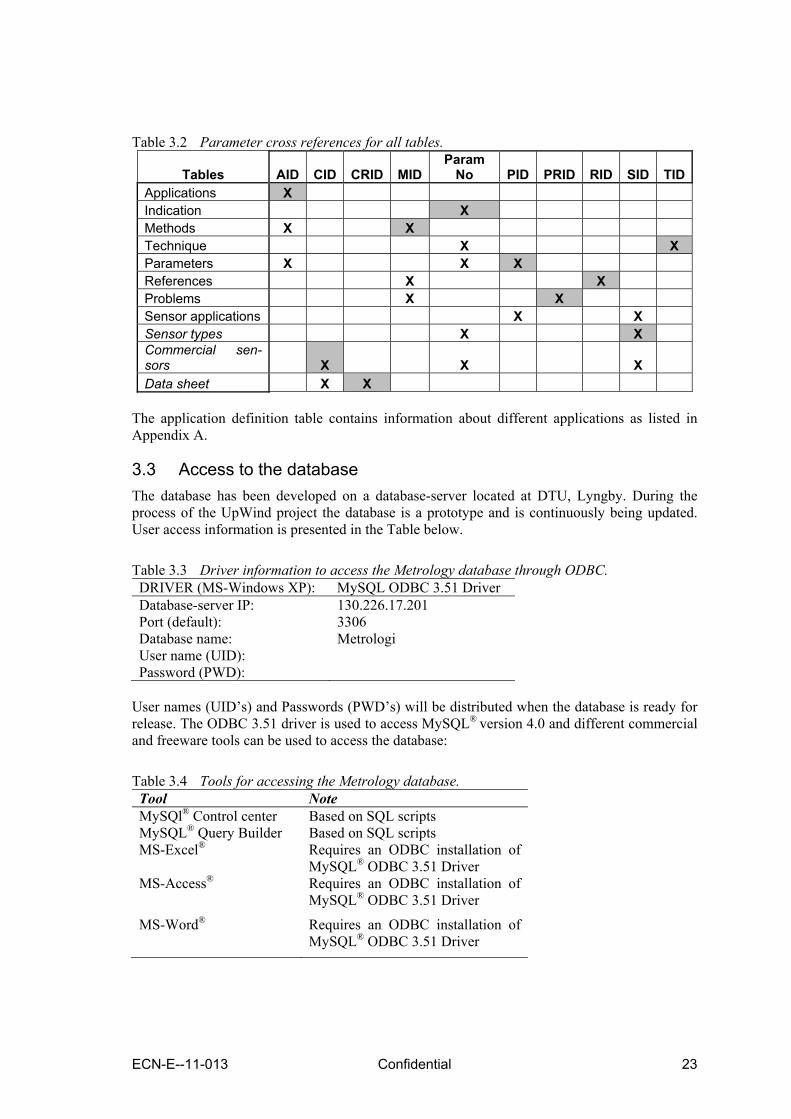
Table 3.2 Parameter cross references for all tables.
Tables AID CID CRID MIDParam
No PID PRID RID SID TIDApplications X Indication X Methods X X Technique X X Parameters X X X References X X Problems X X Sensor applications X X Sensor types X X Commercial sen-sors X X X Data sheet X X
The application definition table contains information about different applications as listed in Appendix A.
3.3 Access to the database The database has been developed on a database-server located at DTU, Lyngby. During the process of the UpWind project the database is a prototype and is continuously being updated. User access information is presented in the Table below.
Table 3.3 Driver information to access the Metrology database through ODBC. DRIVER (MS-Windows XP): MySQL ODBC 3.51 Driver Database-server IP: 130.226.17.201 Port (default): 3306 Database name: Metrologi User name (UID): Password (PWD):
User names (UID’s) and Passwords (PWD’s) will be distributed when the database is ready for release. The ODBC 3.51 driver is used to access MySQL® version 4.0 and different commercial and freeware tools can be used to access the database:
Table 3.4 Tools for accessing the Metrology database. Tool Note MySQl® Control center Based on SQL scripts MySQL® Query Builder Based on SQL scripts MS-Excel® Requires an ODBC installation of
MySQL® ODBC 3.51 Driver MS-Access® Requires an ODBC installation of
MySQL® ODBC 3.51 Driver
MS-Word® Requires an ODBC installation of MySQL® ODBC 3.51 Driver

24 Confidential ECN-E--11-013
Using MS-Access with linked MySQL® tables enables the user to work in a MS-Access envi-ronment but requires access to the Internet. MS-Access® includes all necessary tools for query-ing and reporting the contents of the database. A MS-Excel link enables import of table(s) or queries to a MS-spreadsheet.
Figure 3.2 List of linked tables in MS-Access from the Metrology database.
Figure 3.3 List of predefined, dedicated reports based on linked tables.
ECN-E--11-013 Confidential 25
3.4 Discussion and Conclusions The UpWind consortium research covers a wide area of expertise in wind energy. The required measurement and analysis techniques covering this wide range are identified after successful and extensive interaction between the various work packages of the UpWind project. The second deliverable is to find theoretical solutions for the identified metrology problems. Based on the deliverable 1, the list of measurement problems, it has been analysed what the pre-cise consequences are of the identified problems and in which directions possible solutions can be found. In order to process the large amounts of data, and especially the many relations, a database structure has been designed. A dedicated database is designed to systematically organise the in-formation that has been generated. First of all, the identified measurement problems are in-cluded, the state-of-the-art measurement techniques, including lists of sensors applied to meas-ure the various measurands. Furthermore, a list of commercially available sensors is included. The database has been developed in MySQL, which can be installed on both Linux and MS-Windows personal computers. The metrology database consists of a number of individual ta-bles, which are linked together through a number of variables. The applications from the differ-ent UpWind Work Packages have been used as key parameters and the other tables contain the derived and necessary methods, measurands, techniques, etc. Further work within the work package 1A2 Metrology will concentrate on the further analyses and demonstration of the measurement techniques and analysis techniques.
3.5 References [1] P.J. Eecen, N. Stefanatos, T.F. Pedersen, K.S. Hansen, UpWind METROLOGY. Deliv-
erable D 1A2.2; Metrology Database – Definition, ECN-E--08-079

26 Confidential ECN-E--11-013

ECN-E--11-013 Confidential 27
4. Turbulence normalization combined with the equivalent wind speed method
Rozenn Wagner and Julia Gottschall
4.1 Introduction The power performance of a wind turbine has to be measured according to the IEC 61400-12-1 standard [1]. The power curve is obtained with 10 minute mean power output from the turbine plotted against simultaneous 10 minute average wind speeds. The standard only requires the wind speed the wind speed at hub height and the air density (derived from temperature and pres-sure measurement). However it has been shown that other characteristics of the wind field influ-ence the power performance measurement too. These parameters are the wind shear (see chapter 5 and 6) and the turbulence intensity [1, 2]. Turbulence intensity (TI) is defined as the ratio be-tween 10-minute standard deviation and mean wind speed.
4.2 Effect of the turbulence intensity When the wind speed fluctuates around the rated wind speed, the power extracted is limited to the rated power. Therefore only “negative fluctuations'” (i.e. the instantaneous wind speeds be-low rated speed) of the wind are transformed into power fluctuations. Consequently, 10 minute mean power obtained with a given turbulence intensity is generally smaller than the power that would be obtained with the same mean wind speed and a laminar flow (TI=0%), and the mean power decreases as the turbulence intensity increases, see Figure 4.1. In the same way, as the wind speed fluctuates around the cut-in wind speed, only the positive fluctuations are trans-formed in power fluctuations. Therefore, near the cut-in wind speed, the mean power is ex-pected to increase with the turbulence intensity. Between the cut-in and rated speeds, the turbine is expected to respond to any wind speed fluctuations (positive or negative). Within the wind speed range where the CP is nearly constant, the turbine power increases with the turbulence in-tensity as the power is then proportional to the cube of the wind speed. Moreover, according to BEM simulations (with HAWC2Aero), the scatter increases around the mean power curve with the turbulence intensity.
Figure 4.1 Mean power curves for various turbulence intensities
The effect of the turbulence intensity on the power curve can be seen as the combination of one effect on the mean power curve that varies with the turbulence intensity (especially around rated speed) and one effect on the scatter that increases with the turbulence intensity. The scatter in the power curve results from both effects as it usually results from a distribution of various tur-bulence intensities.

28 Confidential ECN-E--11-013
4.3 Equivalent wind speed and turbulence The effects of turbulence intensity on the power curve cannot be taken into account with a sim-ple definition of equivalent wind speed similar to the one used to account for the shear [2]. Al-bers suggested a method aiming at representing the non linear relation between the 10 minute mean power and the 10 minute mean wind speed [1]. This method is based on the fact that the 10 minute average of the power is not linearly related to the mean wind speed but to the wind speed distribution during the considered 10 minute and the shape of the power curve.
4.4 Description of Albers' method The model is based on the assumption that the wind turbine follows the same power curve at each instant. This power curve is the curve that should be theoretically obtained with 0% turbu-lence intensity. According to this assumption, the power output of the turbine for any turbulence intensity can be simulated by:
sim 0%v=0P (v,TI)= P (v) f(v) dv
∞
∫ (4.1)
where P0%(v) is the power given by the 0%-TI power curve for the wind speed v, and f(v) is the wind speed distribution within the 10 minutes. This distribution is assumed to be Gaussian, de-noted by 2( ) ( , )f v v σ= Ν , it only depends on the 10 minute wind speed average, v, and va-riance, 2σ . The variance here is given by 2 2 2v TIσ = × . Albers' method therefore consists of 2 steps: The estimation of the 0%-TI power curve; The simulation of the power curve for a chosen turbulence intensity: TItarget. Step1: definition of the 0%TI power curve The 0%-TI power curve is derived from a few parameters characteristic of the turbine: the rated power, the cut-in wind speed and the maximum CP [1]. The values taken for these parameters are tuned with an iterative process in order to minimize the error between the simulated mean power curve and the measured mean power curve. The simulated mean power curve is the pow-er curve obtained by applying (4.1) to each wind speed bin (i.e. the wind speed bins used to av-erage the power curve as described in the IEC 61400-12-1 standard) statistics: sim i iP (v ,TI ) where vi is the bin-averaged speed and TIi is the bin-averaged turbulence intensity in the ith bin.
Step2: Simulation of the power output with TItarget Once the 0%-TI power curve has been determined, each 10 minute measured power output is corrected for the TItarget by applying the formula: target
(10) (10) (10) (10) (10) (10) (10)TI meas sim meas target meas sim meas measP (v )=P (v , TI ) + P - P (v , TI ) (4.2)
where (10)
measP and (10)measv are the simultaneous measured 10 minute mean power and wind speed
and (10)measTI is the 10 minute measured TI. (10) (10) (10)( , )sim meas meansP v TI is the power output expected if the
assumption that the turbine follows the 0% TI power curve at each instant was true. But there is actually a difference between the actual power output and the simulated power output as the power curve is influenced by other parameters than the turbulence intensity such as the speed shear for example. Albers' method can only reduce the scatter due to the distribution of the tur-bulence intensity during the power curve measurement. Figure 4.2 shows the measured power curve scatter plot, the simulated power curve for arg 10%t etTI = and the predicted power curve
scatter plot for arg 10%t etTI =

ECN-E--11-013 Confidential 29
Figure 4.2 Measured power curve scatter plot ( (10)
measP ), simulated power output for
target 10%TI = ( (10) (10)sim meas target( , )P v TI ), resulting simulated power curve scatter plot
(arg
(10)t etTIP ).
4.5 Combination with the equivalent wind speed Albers’ method was designed to normalize the standard power curve to a chosen TI: targetTI . On the other hand, the equivalent wind speed method “normalizes” the power curve for the effect of shear, the combination of these two methods would result in a power curve less sensitive to the wind characteristics, and therefore less dependent on the site and season. The turbulence normalisation changes the power value whereas the equivalent wind speed method changes the wind speed. It is therefore quite simple to combine both method in order to obtain a power curve less sensitive to shear and turbulence intensity. Albers' method was initially designed to normalize the standard power curve, i.e. based on wind speed measurements at hub height, for the turbulence intensity. In order to compare the results to those obtained by combining Albers' method with the equivalent wind speed, the turbulence normalisation was applied to both power curves: with hub height wind speed and with equiva-lent wind speed. Therefore for a given targetTI value, four results can be compared:
Measured power Normalized power
uhub Standard power curve Alber’s method
Ueq Equivalent wind speed power curve
Combined method
Figure 4.3 Mean power curve and scatter in the power curve obtained with wind speed
measurements at hub height and equivalent wind speed, both with and without turbulence normalization using Albers' method

30 Confidential ECN-E--11-013
The power curve obtained by combining both the equivalent wind speed and Alber’s turbulence normalization presents both a modification of the shape of the mean power curve (due to the dif-ferent TI) and a reduction of the scatter around the mean power curve (scatter due to the shear).
4.6 Conclusions The equivalent wind speed method reduces scatter due to shear also when the power has been normalized for the turbulence intensity according to Albers' method for turbulence normaliza-tion, except near rated speed where the mean power curve slope is significantly changed. The mean power curve obtained with the combination of both methods is less sensitive to shear and is representative for a given TI. Such a power curve can give a better representation of the power curve that would be obtained at another site, with different wind shears and turbulence intensities from the power curve measurement site. In this sense, it is transferable from one site to another. Therefore it would give a better Annual Energy Production (AEP) estimation.
4.7 References [1] Kaiser K, Hohlen H, Langreder W, Turbulence correction for power curves, EWEC 2008
[2] Albers A, Turbulence normalisation of wind turbine power curve data, EWEC 2010
[3] Wagner R, Accounting for the speed shear in wind turbine power performance measure-ment, PhD thesis (chapters 4 and 9), 2010.

ECN-E--11-013 Confidential 31
5. Improvements in power performance measurement techniques
Jan Willem Wagenaar and Peter Eecen This part of the report focuses on the analyses of the largest sources of uncertainties in power performance testing. The work is directly relevant for work being performed in the context of the IEC61400-12-1 and MEASNET [1]. It is known that the power performance of a wind tur-bine depends on atmospheric conditions as for instance the air density. The IEC regulations for power performance [2] already include an air density correction. Besides that it is also known that other atmospheric conditions play a role as well, such as turbulence and wind shear, which was already noticed in [3]. Other authors notice this dependence as well, such as for instance [4] [5] [6] [7]. Corrections for turbulence and wind shear have been suggested and have been shown to be effective. We examine the power performance of a 2.5MW ECN research turbine on the ECN test field on those atmospheric conditions. A site description is give together with a description of necessary data selection. The dependence of the power performance on the air density, stability, turbu-lence and vertical wind shear is examined in subsequent sections.
5.1 EWTW and Data taking ECN has made available the ‘ECN Wind Turbine test station Wieringermeer’ (EWTW) since the end of 2002. A site description is given in section 5.1.1. Data selection and correction pro-cedures are described in section 5.1.2.
5.1.1 Site description The EWTW is located in the North East of the province North Holland, 3 km North of the town Medemblik and 35 km East of ECN Petten. It consists of research turbines, prototype turbines and scaled wind turbines, all accompanied with meteorological masts. For this work the re-search turbines (green squares) and the nearby meteorological mast (meteo mast 3) are of inter-est and are indicated in Figure 5.1.
-1000
0
1000
2000
-2000 -1000 0 1000 2000
Meteo mast 3
Meteo mast 2 Meteo mast 1
Figure 5.1 Map of EWTW

32 Confidential ECN-E--11-013
The surroundings of the test site are characterized by flat terrain, consisting of mainly agricul-tural area, with single farmhouses and rows of trees. The lake “IJsselmeer” is located at a dis-tance of 1 to 2 km East. For more details see [8]. The 5 research turbines, named T5 – T9 (West to East), are 2.5MW ECN research turbines with a rotor diameter (D) of 80m, a hub height (H) of 80m and a rated power of 2.5MW. The nearby meteorological mast measures, among others, the wind speed and direction at 52m, 80m and 108m, pressure, temperature and temperature difference. A detailed description of the mast can be found in [8]. From now on, if not mentioned differently, the wind speed and direction always refers to the wind speed and direction at 80m. All data taken from the turbines and the meteorological mast are stored in the “Long Term Vali-dation Measurements” (LTVM) database [9] of the Wind Data Management System (WDMS) [10]. This database structure ensures high quality data. Data has been taken from September 2004 until April 2010, which makes it possible to analyse a large amount of data.
5.1.2 IEC Standards and data selection To perform power performance measurements the IEC 61400-12-1 regulations [2] have been followed, where possible. The distance of turbines T5 and T6 to the meteorological mast is such (3.5D and 2.5D, respectively) that these turbines only are close enough to the meteorological mast for power performance measurements. In this work T6 is considered. An undisturbed wind sector is identified by choosing wind directions between 347° - 354°, 126° - 133° and 212° - 244°. Besides the wind direction selection, other obviously erroneous data points are neglected as well. For the entire period of about 6 years of data taking, the power curve of turbine T6 is con-structed and depicted in the upper plot of Figure 5.2. Here, the scatter data as well as the binned values are shown. The lower plot shows the AEP against the reference wind speed. We note that the scatter plot in Figure 5.2 has 3 tails (15-20 m/s), which influences the standard deviation of the “method of bins”. In the remainder different (sub) data sets will be considered and the dis-tribution of the data points for wind speeds above 15m/s over the three ‘tails’ may be different from one situation to another. This influences the power and the standard deviation of the power. Therefore, when comparing the power or the standard deviations of the power, wind speeds above 15m/s are not considered in this chapter.

ECN-E--11-013 Confidential 33
Figure 5.2 Scatter plot (blue) and IEC “method of bins” (red) of power against normalized
wind speed (upper plot). The lower plot contains the AEP as function of the reference wind speed.

34 Confidential ECN-E--11-013
5.2 Atmospheric conditions In this section the dependence of the power curve on atmospheric conditions as air density, tem-perature, stability, turbulence and wind shear is examined. Possible cross correlations are also studied.
5.2.1 Air density The power that a turbine can extract from a volume of wind is [11]
3
21 UAcP p ⋅⋅⋅⋅= ρ , ( 5.1 )
where U is the horizontal wind speed, A is the rotor swept area, ρ is the air density and cp is the power coefficient. P is the power. Clearly, the power depends on the air density and therefore also the power curve. In this section we want to see to what extend the power curve depends on the air density. Before studying this effect of air density Figure 5.3 shows the distribution of the encountered air density values1. It is noticed that most values lay between 1.20 kg/m3 and 1.27 kg/m3. The mean value is 1.237 kg/m3.
Figure 5.3 Distribution of the air density.
1 The air density distribution is extracted from the same data set as used for the power performance. This will also be valid for the distributions of other atmospheric quantities.

ECN-E--11-013 Confidential 35
Figure 5.4 Power as function of the (not normalized) wind speed for various values of the air density (upper plot). Difference between the power for all values of the air density and the power for various values of the air density as function of the (not normalized) wind speed (lower plot).
Power curves for various values of the air density are shown in the upper plot of Figure 5.4. They can clearly be distinguished. The lower plot shows the difference between the power for all values of the air density and the power for various values of the air density. The maximum difference occurs for the power curve for ρ=1.205 kg/m3. This difference is at most 4% for (not normalized) wind speeds above 5m/s. Also for different values of temperature power curves can be distinguished. However, because the air density is calculated from temperature (and pressure) measurements, it is obvious that the two are related. This is also reflected in the power curves.
5.2.2 Stability The stability of the atmosphere is determined by means of the environmental lapse rate: -dT/dh < 6K/km = stable atmospheric conditions 6K/km < -dT/dh < 10K/km = conditionally unstable atmospheric conditions -dT/dh > 10K/km = unstable atmospheric conditions, where T is the temperature and h is the height. Here, the lapse rate is determined using the tem-perature difference instrument, which measures the temperature difference between a height of 37m and 10m. The distribution of the stability is exposed in Figure 5.5. It is clearly seen that unstable conditions happen the most during daytime and during summer. For stable conditions the opposite is valid.

36 Confidential ECN-E--11-013
Figure 5.5 Normalized frequency of occurrence of different stability conditions as function of the hour of the day (upper plot) and as function of the month of the year (lower plot).
Within the considered period stable conditions occur the most: the number of data points with stable conditions is about 7 times higher than the number of data points with conditionally sta-ble or unstable conditions. The power curves for stable, unstable and all atmospheric conditions are given in Figure 5.6, as are the relative differences and the relative differences in the standard deviation. For wind speeds above, say, 6m/s the difference between the power for all atmospheric conditions and stable conditions and the between the power curve all atmospheric conditions and unstable con-ditions is lower than about 4%. More interesting are the differences in the standard deviation of the power. Again we consider the wind speed range 4m/s – 13m/s. We see that the standard deviation for unstable conditions is up to 50% larger than the standard deviation for all conditions. Furthermore the standard deviation for stable conditions is smaller (~10%) than the standard deviation for all conditions.

ECN-E--11-013 Confidential 37
Figure 5.6 Power curve (upper plot) for different stability conditions. Relative difference in
power (lower left plot) between all and stable conditions (blue) and between all and unstable conditions (red). Relative difference in standard deviation (lower right plot) between all and stable conditions (blue) and between all and unstable conditions (red).

38 Confidential ECN-E--11-013
5.2.3 Turbulence The turbulence intensity is defined as [3]
UTI Uσ= , ( 5.2 )
where σU is the standard deviation of the wind speed. We note here that occasionally the turbu-lence intensity is exposed as a percentage. In that case (5.2) is multiplied with 100. In Figure 5.7 the distribution of the turbulence intensity (in percentage) is given. It is seen that most values are between 2% and 12% and the mean is 8.1%. It is also seen that the TI is some-what higher during daytime.
Figure 5.7 Normalized frequency of occurrence of the turbulence intensity (upper plot).
Normalized frequency of occurrence of the turbulence intensity as function of the hour of the day (middle plot). Normalized frequency of occurrence of the turbulence intensity as function of the month of the year (lower plot).
The power curve for different turbulence intensity classes is given in Figure 5.8, as are the rela-tive differences and the relative differences in the standard deviation. As noticed before [12] we see that for low wind speeds (4m/s-10m/s) high TI classes yield the most power and for high wind (12m/s-14m/s) speeds low TI classes yield the most power. Also, differences in the stan-dard deviations of the power are clearly seen. In the wind speed range 6m/s – 13m/s we see that the standard deviation of certain turbulence intensity classes (4%-6% and 12%-14%) differ up to about 50% with the standard deviation for all turbulence intensities. Furthermore, it is noticed that the standard deviation of the power for high turbulence intensities is larger than the stan-dard deviation of the power for all turbulence intensities up to wind speeds of 10m/s. For low turbulence intensities the opposite is valid.

ECN-E--11-013 Confidential 39
Figure 5.8 Power curve (upper plot) for different turbulence intensity classes. Relative differences in power (lower left plot) between all and various TI classes. Relative difference in standard deviation (lower right plot) between all and various TI classes.
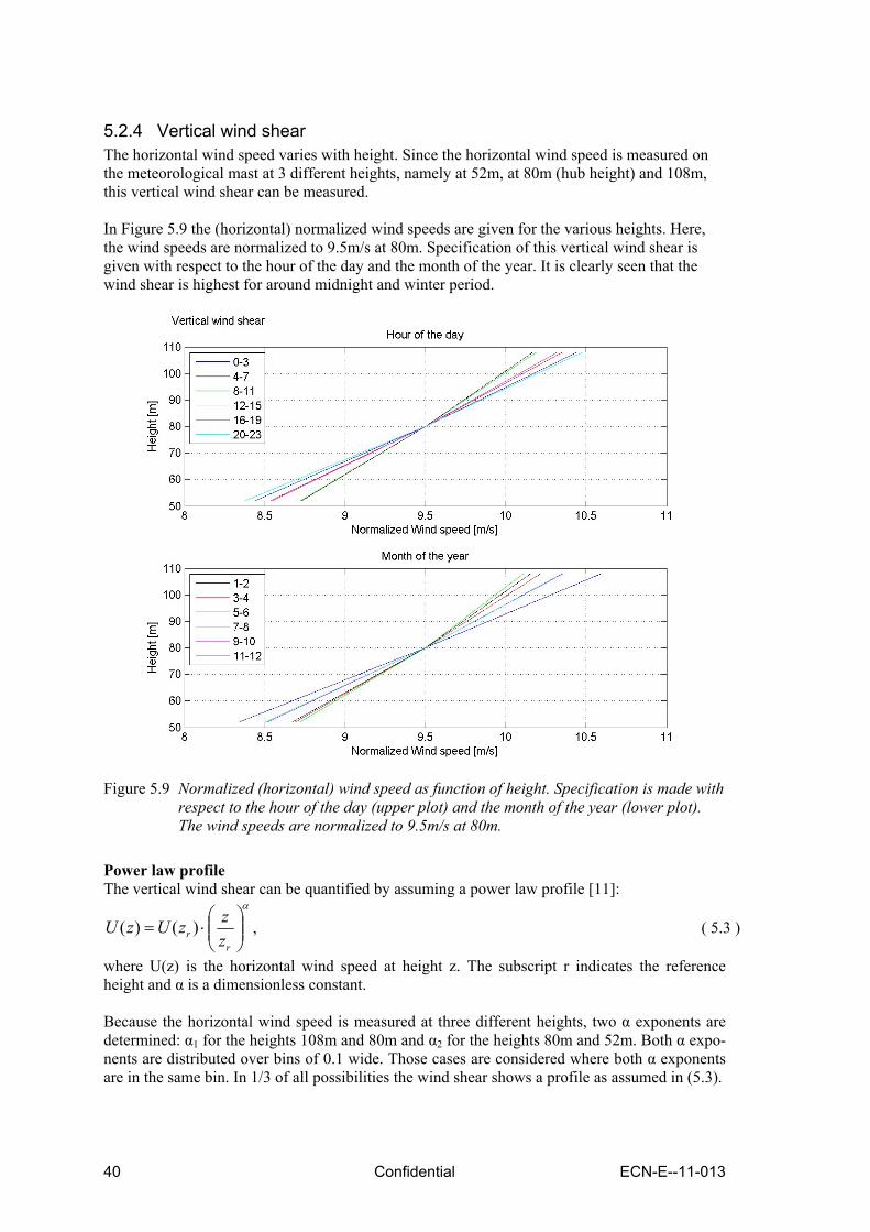
40 Confidential ECN-E--11-013
5.2.4 Vertical wind shear The horizontal wind speed varies with height. Since the horizontal wind speed is measured on the meteorological mast at 3 different heights, namely at 52m, at 80m (hub height) and 108m, this vertical wind shear can be measured. In Figure 5.9 the (horizontal) normalized wind speeds are given for the various heights. Here, the wind speeds are normalized to 9.5m/s at 80m. Specification of this vertical wind shear is given with respect to the hour of the day and the month of the year. It is clearly seen that the wind shear is highest for around midnight and winter period.
Figure 5.9 Normalized (horizontal) wind speed as function of height. Specification is made with
respect to the hour of the day (upper plot) and the month of the year (lower plot). The wind speeds are normalized to 9.5m/s at 80m.
Power law profile The vertical wind shear can be quantified by assuming a power law profile [11]:
α
⎟⎟⎠
⎞⎜⎜⎝
⎛⋅=
rr z
zzUzU )()( , ( 5.3 )
where U(z) is the horizontal wind speed at height z. The subscript r indicates the reference height and α is a dimensionless constant. Because the horizontal wind speed is measured at three different heights, two α exponents are determined: α1 for the heights 108m and 80m and α2 for the heights 80m and 52m. Both α expo-nents are distributed over bins of 0.1 wide. Those cases are considered where both α exponents are in the same bin. In 1/3 of all possibilities the wind shear shows a profile as assumed in (5.3).
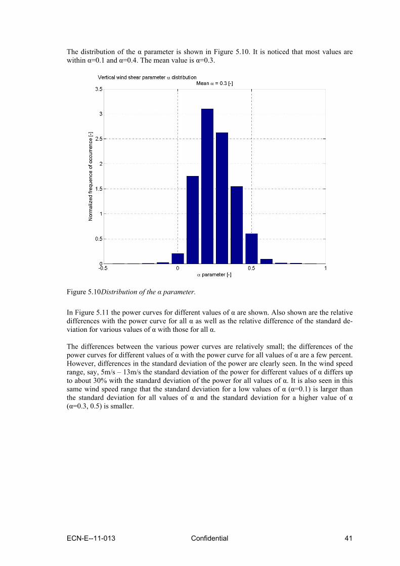
ECN-E--11-013 Confidential 41
The distribution of the α parameter is shown in Figure 5.10. It is noticed that most values are within α=0.1 and α=0.4. The mean value is α=0.3.
Figure 5.10 Distribution of the α parameter.
In Figure 5.11 the power curves for different values of α are shown. Also shown are the relative differences with the power curve for all α as well as the relative difference of the standard de-viation for various values of α with those for all α. The differences between the various power curves are relatively small; the differences of the power curves for different values of α with the power curve for all values of α are a few percent. However, differences in the standard deviation of the power are clearly seen. In the wind speed range, say, 5m/s – 13m/s the standard deviation of the power for different values of α differs up to about 30% with the standard deviation of the power for all values of α. It is also seen in this same wind speed range that the standard deviation for a low values of α (α=0.1) is larger than the standard deviation for all values of α and the standard deviation for a higher value of α (α=0.3, 0.5) is smaller.

42 Confidential ECN-E--11-013
Figure 5.11 Power for different values of α (upper plot), relative difference in power (lower left
plot) between all and various values of α and relative difference in σ of power (lower right plot) between all and various values of α as function of the normalized wind speed.
Linear profile Here, the vertical wind shear is quantified by assuming a linear profile:
RzzzUzU r
r−
⋅+= β)()( , ( 5.4 )
Where β is the coefficient determining the steepness of the linear profile. All other symbols are as before. The inclusion of the rotor radius R is to make the parameter β have the same dimen-sion as the wind speed (m/s). Again, two β coefficients can be determined based on measurements at three different heights. Both β coefficients are distributed over bins of 0.1 wide. Those cases are considered where both coefficients are in the same bin. In 40% of all possibilities the wind shear shows a profile as as-sumed in (5.4). The distribution of the β coefficient is shown in Figure 5.12. It is noticed that most values are within β=0.5m/s and β=2m/s. The mean value is β=1.25m/s.

ECN-E--11-013 Confidential 43
Figure 5.12 Distribution of the β parameter.
In Figure 5.13 the power curves and the standard deviation of the power for different values of β are shown. Also shown are the relative differences with the power curve for all β as well as the relative difference of the standard deviation for various values of β with those for all β. It is seen that the power for β values of 1m/s-2m/s is at most about 10% larger at a wind speed of 5m/s with respect to the power for all values of β. Furthermore, it is seen that the standard deviation of the power for lower values of β (0.5m/s-1m/s) is up to 50% higher than the stan-dard deviation for all values of β. For higher values of β the standard deviation is lower than the standard deviation for all values of β.

44 Confidential ECN-E--11-013
Figure 5.13 Power (upper left plot) and σ of power (upper right plot) for different values of β,
relative difference in power (lower left plot) between all and various values of β and relative difference in σ of power (lower right plot) between all and various values of β as function of the normalized wind speed.
5.2.5 Cross correlations Although stability, turbulence and vertical wind shear are treated separately in the foregoing, it may be expected that these phenomena are correlated. Therefore, Figure 5.14 shows the distri-bution of the α parameter for different stability conditions and for different TI classes. Also shown are the vertical wind speed profiles for different stability conditions and for different TI classes. The β parameter is not considered in this analysis of correlation. From the distribution of α for different stability conditions it is clearly seen that the value of α that occurs the most for unstable conditions is α=0.1. For stable conditions this is α=0.3. It is also seen that the distribution of α for unstable conditions is sharper then for stable conditions. From the distribution of α for different turbulence intensities a sharp distribution of α is seen for high TI, centred around α=0.1. The value of the α parameter that occurs the most for low TI is α=0.4. These phenomena are explained by the fact that for unstable conditions and high turbu-lence different layers of air mix, which increases the correlation of the horizontal wind speeds at different heights. This decreases the value of α and broadens the distribution. For a value of α=0 all horizontal wind speeds at different heights are the same. This mixing of air layers is also reflected in the vertical wind shear profiles (lower plots of Fig-ure 5.14), where a low wind shears are seen for unstable conditions and high turbulence.

ECN-E--11-013 Confidential 45
Figure 5.14 Distribution of α for different stability conditions (upper left plot) and different TI
(upper right plot). Wind shear profiles for different stability conditions (lower left plot) and different TI (lower right plot).

46 Confidential ECN-E--11-013
5.3 Power Curve Corrections In the previous section we have shown that the power curve depends on different atmospheric conditions as stability, turbulence and wind shear. In this section we study correction of these effects on the power curve. We have not found a correction with respect to stability, however, as we have shown, stability is correlated to turbulence and wind shear. Therefore we study correc-tion with respect to turbulence and wind shear, only.
5.3.1 Air density Because the turbine is a pitch-regulated machine an air density correction is performed on the wind speed
3/1
0⎟⎟⎠
⎞⎜⎜⎝
⎛⋅=ρρUU norm . ( 5.5 )
Here, U is the measured wind speed. ρ is the air density, derived from pressure and temperature measurements ([2]) and ρ0 is the reference air density. The effect of the normalization is depicted in Figure 5.15. The upper plots show power curves for different values of the air density, where the left plots is before and the right plot is after cor-rection. From the upper left plot clear differences in the power curves are seen for different val-ues of the air density. It is also clear from the upper right plot that the corrected power curves for different values of the air density are closer together. The wind speed range 9m/s – 14m/s is shown, because in this range the effect is best seen. It is concluded that the dependence of the power curve on the air density is reduced by using (5.5). This point is further illustrated in the lower plots of Figure 5.15. The left plot shows the relative difference in normalized and unnormalized power. The difference is at most 2% -3%. More im-portantly the lower right plot shows the relative difference in the standard deviation of the power. It is clearly seen that the standard deviation is reduced by means of the correction (5.5) in the wind speed range 4m/s – 13m/s. In this range the cubic dependence of the power on the wind speed is most pronounced and (5.5) is here most effective. A reduction of the standard de-viation of about 9% is seen.

ECN-E--11-013 Confidential 47
Figure 5.15 Power curves for different values of the air density before (upper left plot) and
after (upper right plot) air density correction. Relative difference in normalized and unnormalized power as function of the normalized wind speed (lower left plot). Relative difference in normalized and unnormalized standard deviation of the power as function of the normalized wind speed (lower right plot).
As mentioned before temperature and air density are correlated. Therefore air density correction is implicitly also temperature correction. It is indeed observed that the air density correction is also effective for reducing the dependence of the power curve on the temperature. Nevertheless, a small influence of the temperature on the power curve remains, as is the case for the air den-sity.
5.3.2 Turbulence 1D Turbulence In (2) it is shown that the power depends cubically on the wind speed. Implicitly, the third power of the averaged wind speed was considered. However, the average of the power depends on the average of the cubed wind speed. It can be shown [6] that in this way a correction factor is added or, equivalently, a corrected wind speed is defined
3/12
31 ⎟⎟⎠
⎞⎜⎜⎝
⎛⎟⎠⎞
⎜⎝⎛⋅+⋅=
UUU U
normcorrσ
. ( 5.6 )
Here, σU/U is the TI (5.2). The turbulence corrected power is shown in Figure 5.16 for different values of TI. Also shown is the uncorrected power for different values of TI (as in Figure 5.8) for comparison. The vari-ous curves are in the corrected case somewhat closer together with respect to the uncorrected case. This is made more quantitative in the relative difference in the standard deviation of the power before and after the correction. Here, the standard deviation of the corrected power is for almost all wind speeds in the range up to 12m/s lower than the standard deviation of the uncor-

48 Confidential ECN-E--11-013
rected power. A reduction up to 9% is seen. The correction (5.6) is based on the cubical depend-ence of the power on the wind speed. This behaviour is most pronounced in the mentioned wind speed range. Therefore, it is concluded that the turbulence correction (5.6) is effective. A difference in power is seen up to 7%; above 6m/s this is at most 2%. For almost all wind speeds the corrected power is lower than the uncorrected power. This is caused by the fact that the corrected wind speed is always larger that the uncorrected wind speed.
Figure 5.16 Power for different values of TI as function of the normalized wind speed (upper left
plot) and the TI corrected wind speed (upper right plot). Relative difference in power (lower left plot) before and after TI correction. Relative difference in σ of power (lower right plot) before and after TI correction.
3D Turbulence Taking 3D turbulence into account, it can be shown [4] that a 3D turbulence corrected wind speed is defined as follows
3/12
51 ⎟⎟⎠
⎞⎜⎜⎝
⎛⎟⎠⎞
⎜⎝⎛⋅+⋅=
UUU U
normcorrσ
. ( 1.7 )
Here, isotropic turbulence is assumed and yaw misaligned and vertical inflow is neglected. The relative change in the standard deviation of the power as a result of the correction in (5.7) is shown in Figure 5.17. Below 10m/s a decrease in the standard deviation of the power is seen; an even stronger decrease than was seen in the 1D case. At 4m/s the decrease is 10%. Above 10m/s we see an increase in standard deviation. This increase is even stronger than in the 1D case. It is mentioned that the correction (5.7) is based on the cubic dependence of the power curve on the wind speed. This is in any case not valid above 12m/s.

ECN-E--11-013 Confidential 49
The relative change in power is at most about 9% and for all cases the corrected power is smaller than the uncorrected power, as was the case in the 1D case. However, in this case the difference is larger, i.e. we see a larger deviation from the uncorrected situation. For wind speeds above 6m/s the change in power is at most 3-4%.
Figure 5.17 Relative difference in standard deviation of power before and after TI correction (6).
5.3.3 Vertical wind shear: Wind speed corrections To correct for the wind shear various approaches are considered. The first approach is to di-rectly use the measurements at multiple heights in a redefinition of the wind speed. Other ap-proaches are to determine vertical wind shear profile based on these measurements and to cor-rect the wind speeds according to these profiles. A power law and a linear profile is considered. Multiple measurements The measurements at the various heights are used in a redefinition of the wind speed: the so-called rotor averaged wind speed
( )108108808052521 UAUAUAA
U averagedrotor ⋅+⋅+⋅=− , ( 5.8 )
Here, Ui (i=52, 80 and 108) is the wind speed at height i. A is the entire rotor swept area and A52, A80 and A108 are different sections of this area defined by height x
2RA π=
42arcsin2
222
80xRx
RxRA −⋅+⎟⎠⎞
⎜⎝⎛⋅⋅= , ( 5.9 )
280
10852AA
AA−
==

50 Confidential ECN-E--11-013
where R=D/2=40m. The meaning of these entities becomes clear when looking at Figure 5.18.
Figure 5.18 Rotor swept area divided in three sections.
We notice that for x=80m the rotor averaged wind speed is equal to the wind speed at hub height. So, no correction takes place. The rotor averaged wind speed corrected power is shown in Figure 5.19 for different values of x. Also shown are the relative difference between the corrected (x dependent) and the uncor-rected power (x=80m) as well as the relative difference in the standard deviation of the cor-rected and uncorrected power. The different corrected power curves differ only up to 4% for wind speeds above 4m/s from the uncorrected power curve. In practically all cases (all x-values and wind speeds) the corrected power is larger than the uncorrected power. Based on Figure 5.19, only for x=60m the standard deviation of the power shows for most wind speeds a decrease about 3%. In practice, for values of x above 50m the standard deviation of the power is decreased of about a few percent. There-fore, this correction is only effective for these values of x, although the effect is relative small.

ECN-E--11-013 Confidential 51
Figure 5.19 Power curve for various values of x (upper plot). Relative difference in power with
respect to the power at x=80m as function of the rotor averaged wind speed for various values of x (lower left plot). Relative difference in standard deviation of power with respect to the standard deviation at x=80m as function of the rotor averaged wind speed for various values of x (lower right plot).
Power law profile Further attempts to correct for vertical wind shear are sought in the assumption of a power law profile of the wind shear. Here, we first average the (horizontal) wind speed vertically
⎟⎟⎠
⎞⎜⎜⎝
⎛⎟⎠⎞
⎜⎝⎛−⎟
⎠⎞
⎜⎝⎛⋅
+⋅==
+++
−∫
11
, 21
23
11)()(
21 αα
α αHUdzzU
RU
RH
RHvertical , ( 5.10 )
where U(z) is defined in (5.3) and zr = H. Furthermore, it has been used that H=2R. From (5.10) it is obvious that the hub height wind speed U(H) is α corrected based on the profile it is experi-encing. These corrections are in the range 0.989 - 1.0353 for the α values in the range -0.5 to 1. A second possibility is to average the wind speed over the rotor plane [5]. Again, a power law wind profile is assumed (5.3)
dyyyHUdAzUA
URH
RHrotor
α
α π⎟⎠⎞
⎜⎝⎛ +⋅−⋅⋅== ∫∫
−
+
−
12
12)()(1 1
1
2, , ( 5.11 )
where y is a dummy integration variable. Also in this case the hub height wind speed is α cor-rected based on the profile it is experiencing. Now, the corrections are in the range 0.9918 - 1.0259 for the same α range as before. The results of this vertically averaging and rotor averaging of the wind speed are shown in Fig-ure 5.20. Here, the relative difference between the corrected and the uncorrected power is

52 Confidential ECN-E--11-013
shown as well as the relative difference in the standard deviation of the corrected and uncor-rected power. Both corrections have more are less the same effect. The corrected power differs 12% from the uncorrected power at 4m/s. At higher wind speeds (>6m/s) the difference is at most 4% percent. In all cases the corrected power is larger than the uncorrected power. For most wind speeds a decrease of the standard deviation of at most 10% is seen as a result of the α correction. However, for some wind speeds in this regime an increase is seen.
Figure 5.20 Relative difference in power (upper plot) before and after vertical averaged wind
speed correction (blue) and rotor averaged wind speed correction (red). Relative difference in standard deviation of power (lower plot) before and vertical averaged wind speed correction (blue) and rotor averaged wind speed correction (red).
Linear profile Averaging the wind speed vertically or over the rotor plane assuming a linear wind shear profile (5.4) does not yield a correction factor to the hub height wind speed
)()(21
, HUdzzUR
URH
RHvertical == ∫
+
−β , ( 5.22 )
)()(1, HUdAzU
AU
RH
RHrotor == ∫
+
−β . ( 5.33 )
Therefore, with this set-up no corrected power curves can be obtained. However, we will come back to the point of linear profiles in the next subsection.

ECN-E--11-013 Confidential 53
5.3.4 Vertical wind shear: Power corrections In the previous subsection the focus for correcting for wind shear has been on the wind speed itself. However, here we want the focus to be on the power that can be extracted from that wind, which is
∫⋅⋅⋅= dAzUcP p )(21 3ρ , ( 5.44 )
where the infinitesimal surface element dA is also a function of the height z. With this approach we are going to consider multiple measurements and wind shear profiles, again. Multiple measurements Based on (5.14) it is shown that multiple measurements are used to correct the cube of the wind speed. A redefinition is obtained as follows
3/13108108
38080
35252
,
3,
33
21
21)(
21
⎟⎟⎠
⎞⎜⎜⎝
⎛ ⋅+
⋅+
⋅=
⋅⋅⋅⋅≡
⋅⋅⋅=⋅⋅⋅=
−
−
∑∫
AUA
AUA
AUA
U
UAcP
UAcdAzUcP
cubeaveragedrotor
cubeaveragedrotorp
ii
ipp
ρ
ρρ
. ( 5.55 )
The results of this redefinition are shown in Figure 5.21. It is seen that for the x values shown the power is decreased up to about 7% at 4m/s; for wind speeds above 6m/s this is less than 1%. For almost all wind speeds up to 15 m/s the corrected standard deviation is decreased for x val-ues above 40m. This decrease is at most 5%, which is of the same order, but a bit more as in the linear case (section 5.3.3). So, the correction based on (5.15) (cubically) is a bit more effective than the correction based on (5.8) (linearly).

54 Confidential ECN-E--11-013
Figure 5.21 Relative difference in power with respect to the power at x=80m as function of the
rotor averaged wind speed for various values of x (upper plot). Relative difference in standard deviation of power with respect to the standard deviation at x=80m as function of the rotor averaged wind speed for various values of x (lower plot).
Power law profile The approach started in (5.14) can be applied assuming a power law profile, for which an α cor-rected wind speed is defined
3/131
1
2
3/1
3, 1
212)()()(1
⎟⎟⎠
⎞⎜⎜⎝
⎛⎟⎠⎞
⎜⎝⎛ +⋅−⋅=⎟⎟
⎠
⎞⎜⎜⎝
⎛= ∫∫
−
+
−
dyyyHUzdAzUA
URH
RHcube
α
α π. ( 5.66 )
Again, we see that the hub height wind speed is α corrected. In Figure 5.22 these corrections are shown as function of the wind shear parameter α. Also shown are the corrections obtained in section 5.3.3, equations (5.11), for comparison. The blue line indicates the correction due to the linearly averaging the wind speed over the rotor plane (5.11) and the red line is the correction due to cubically averaging the wind speed over the rotor plane (5.16). As can be seen from Fig-ure 5.10 most values of α are within 0 and 0.5. In this range the corrections differ only a few percent.

ECN-E--11-013 Confidential 55
Figure 5.22 Correction factors to the hub height wind speed as a result of the wind shear
correction based on a power law profile. Distinction is made between the linear wind speed (blue) and the cube of the wind speed (red).
The result of the wind shear correction (5.16) to the power (upper plot) and the standard devia-tion of the power (lower plot) are shown in Figure 5.23. Also shown is the correction due to (5.11). As indicated the blue lines are the corrections as a result of averaging the wind linearly and the red lines are the corrections as a result of averaging of the cube of the wind speed. Regarding the standard deviation of the power we see that the difference between linear averag-ing or cubically averaging the wind speed is small, i.e. the effect of cubically correcting the wind speed is the same as linearly correcting the wind speed. Therefore, with respect to the standard deviation of the power, the same conclusions can be drawn for the effect of the wind shear correction based on a power law profile as in section 5.3.3. A clear difference with respect to the change in power is seen between linearly averaging the wind speed and cubically averaging the wind speed. In the latter case we see that the corrected power generally is about 1% smaller than the uncorrected power for wind speeds above 4m/s. The linear averaged wind speed correction causes the power to be larger with respect to the un-corrected case.
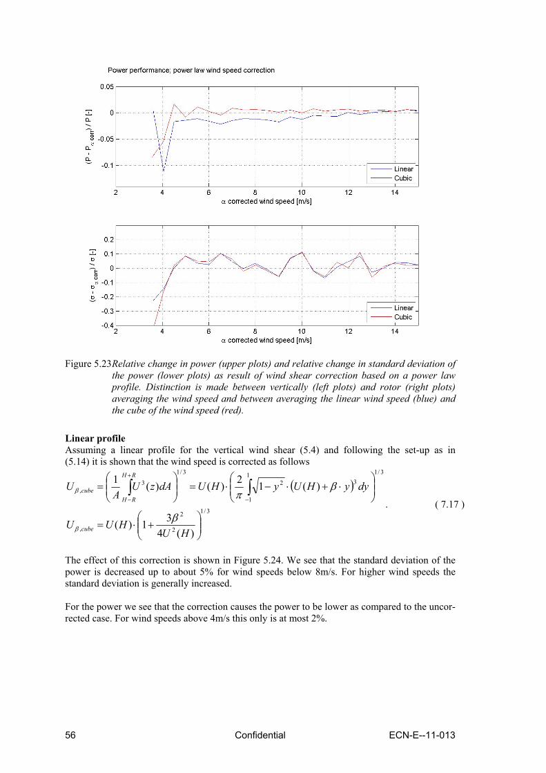
56 Confidential ECN-E--11-013
Figure 5.23 Relative change in power (upper plots) and relative change in standard deviation of
the power (lower plots) as result of wind shear correction based on a power law profile. Distinction is made between vertically (left plots) and rotor (right plots) averaging the wind speed and between averaging the linear wind speed (blue) and the cube of the wind speed (red).
Linear profile Assuming a linear profile for the vertical wind shear (5.4) and following the set-up as in (5.14) it is shown that the wind speed is corrected as follows
( )
3/1
2
2
,
3/13
1
1
2
3/1
3,
)(431)(
)(12)()(1
⎟⎟⎠
⎞⎜⎜⎝
⎛+⋅=
⎟⎟⎠
⎞⎜⎜⎝
⎛⋅+⋅−⋅=⎟⎟
⎠
⎞⎜⎜⎝
⎛= ∫∫
−
+
−
HUHUU
dyyHUyHUdAzUA
U
cube
RH
RHcube
β
βπ
β
β
. ( 7.17 )
The effect of this correction is shown in Figure 5.24. We see that the standard deviation of the power is decreased up to about 5% for wind speeds below 8m/s. For higher wind speeds the standard deviation is generally increased. For the power we see that the correction causes the power to be lower as compared to the uncor-rected case. For wind speeds above 4m/s this only is at most 2%.

ECN-E--11-013 Confidential 57
Figure 5.24 Relative change in power (upper plot) and relative change in standard deviation of
the power (lower plot) as result of wind shear correction based on a linear profile.
5.4 Conclusions All atmospheric conditions that have been considered, i.e. air density, temperature, turbulence and vertical wind shear, have been shown to have effect on either the power curves themselves or on the standard deviation of the power. Corrections with respect to air density, as prescribed by [1], turbulence and vertical wind shear are examined. Corrections with respect to temperature and stability are not considered. This be-cause temperature is correlated to air density and stability is correlated to turbulence and wind shear, as we have seen. Correction with respect to air density and turbulence (1D and 3D) have been shown to be effec-tive for (most) wind speeds in the range where the cubic dependence of the power on the wind speed is most pronounced, say 4m/s - 12m/s. In case of the air density the standard deviation is reduced up to about 8% and in case of the turbulence a reduction up to about 9% (1D) and 10% (3D) is seen. For the 3D turbulence correction the standard deviation of the power is increased above 10m/s. The air density correction and the 1D and 3D turbulence corrections cause the power to be lower than the uncorrected power. For the air density correction and the 1D turbu-lence correction these differences are at most 2% above 6m/s. For the 3D turbulence correction these are at most 3-4% above 6m/s. In case of the rotor averaged wind speed correction, only for x values above 50m an improve-ment in the standard deviation is seen of about 3% in the linear case. In the cubic case the stan-dard deviation is decreased up to 5% for x>40m. The effect of the corrections are considered to be small. In practically all cases (all x-values and wind speeds) the corrected power is larger than the uncorrected power. The difference is at most 4% above 4m/s in the linear case and less

58 Confidential ECN-E--11-013
than 1% above 6m/s in the cubic case. The corrections in the cubic case are slightly better as compared to the linear case. Both (linear) vertical wind shear corrections based on the α parameter basically show the same result. In the most interesting wind speed regime the standard deviations are in most cases re-duced up to about 10%, but for some wind speeds an increase of the standard deviation is seen. The increase in power is at most 4% for wind speeds above 6m/s. Also considered is the vertical wind shear correction based on cubically averaging the wind speed over the rotor plane assum-ing a power law profile. The effect of this correction on the standard deviation is basically the same as for linear averaging over the rotor plane. The change in power is however much less, this is at most (+/-) 1% for wind speeds above 5m/s. The last vertical wind shear correction is to average the wind speed (cubically) over the rotor plane assuming a linear profile. The effect of this correction on the standard deviation of the power is that it is decreased up to about 5% for wind speeds below 8m/s. For higher wind speeds the standard deviation is generally increased. For the power we see that the correction causes the power to be lower as compared to the uncorrected case. For wind speeds above 4m/s this is at most 2%.
5.5 References [1] MEASNET - International Network for Harmonised and Recognised Measurements in
Wind Energy. [2] “IEC 61400-12-1:2005(e): Wind turbines - Part 12-1: Power performance measurements
of electricity producing wind turbines,” 2005. [3] Elliott and Cadogan, “Effects of wind shear and turbulence on wind turbine power
curves,” Proceedings European Community Wind Energy Conference, 1990. [4] Pedersen, Gjerding, Ingham, Enevoldsen, Hansen, and Jorgensen, “Wind turbine power
performance verification in complex terrain and wind farms,” Riso Report, April 2002. Riso-R-1330(EN).
[5] Sumner and Masson, “Influence of atmospheric stability on wind turbine power per-formance curves,” Journal of Solar Energy Engineering, vol. 128, 2006.
[6] Antoniou, Wagner, Pedersen, Paulsen, Madsen, Jorgensen, Thomsen, Enevoldsen, and Thesbjerg, “Influence of wind characteristics on turbine performance,” Proceedings EWEC, 2007.
[7] Rareshide, Tindal, Johnson, Graves, Simpson, Bleeg, Harris, and Schoborg, “Effects of complex wind regimes on turbine performance,” Proceedings AWEA Windpower, 2009.
[8] P. J. Eecen and J. P. Verhoef, “EWTW Meteorological database. Description June 2003 - May 2007,” ECN Report, June 2007. ECN-E–07-041.
[9] Eecen, Machielse, Braam, and Verhoef, “LTVM statistics database,” ECN Report, 2005. [10] D. H. van Dok, Wind Data Management System, Reference Manual. ECN TS&C, re-
lease 3, version 99, k.3718-gr 05/05 ed., 2005. [11] Manwell, McGowan, and Rogers, Wind Energy Explained; Theory, Design and Applica-
tion. Wiley, 2002. [12] Kaiser, Hohlen, and Langreder, “Turbulence correction for power curves,” Proceedings
EWEC, 2003.

ECN-E--11-013 Confidential 59
6. Power performance measurement
Rozenn Wagner
6.1 Influence of shear - Introduction Power performance measurement is central to the wind industry since it forms the basis for the power production warranty of the wind turbine. The power curve measurement has to be rea-lized according to the IEC 61400-12-1 standard [1]. The power curve is obtained with 10 mi-nutes mean power output from the turbine plotted against simultaneous 10 minutes average wind speeds. The standard requires the wind speed to be measured by a cup anemometer mounted on top of a mast having the same height as the turbine hub and located at a distance equivalent to 2.5 rotor diameters from the turbine.
Such a plot usually shows a significant spread of values and not a uniquely defined function. The origin of the scatter can mainly be grouped to four categories: the wind turbine operation and maintenance, lack of correlation due to mast distance, sensor uncertainties and the wind characteristics. Within the last group, the current standard only requires the wind speed at hub height and the air density measurement. However, other wind characteristics can influence the power production like the variation of the wind speed with altitude (i.e. wind speed shear). The influence of wind speed shear on the power performance was shown in several studies: some based on aerodynamic simulations [2] others based on measurements [3],[4]. A major issue is to experimentally evaluate the wind speed shear. The wind speed profile is usually assumed to follow one of the standard models such as the logarithmic or power law pro-files. However, these models are true for some particular meteorological conditions, and there-fore they cannot represent all the profiles that can be experienced by a wind turbine. Measure-ments are then a better option but are also challenging. Indeed characterizing the speed profile in front of the rotor of a multi-megawatt wind turbine requires measurements of wind speed at several heights, including some above hub height, i.e. typically above 100m. Remote sensing instrument such as Lidar or Sodar then appear as a very attractive solution. This chapter starts with a description of the influence of the speed shear on the power perfor-mance of a multi-megawatt turbine. The challenge of describing the speed profile is then dis-cussed followed by a description of an experiment using a Lidar to characterize the speed pro-file. This is followed by the introduction of the definition of an equivalent wind speed taking the wind shear into account resulting in an improvement of the power performance measurement. Finally, some recommendations about remote sensing instruments are given to successfully ap-ply this method.
6.2 Shear and turbine aerodynamics When the flow is axial and homogeneous, i.e. the wind speed is the same at any point, the wind speed seen from a given point on one of the wind turbine blades is the same for any azimuth po-sition. The angle of attack and the relative wind speed are therefore independent on the blade azimuth position (the nacelle tilt is ignored for simplification here), and so is the resulting tan-gential force. On the contrary, if the flow in front of the turbine presents a shear (vertical varia-tion of the horizontal wind speed), the wind speed seen by a given point on a rotating blade va-ries with the azimuth position of the blade, so does the tangential force on all blades which af-fects the resulting torque, see Figure 6.1.
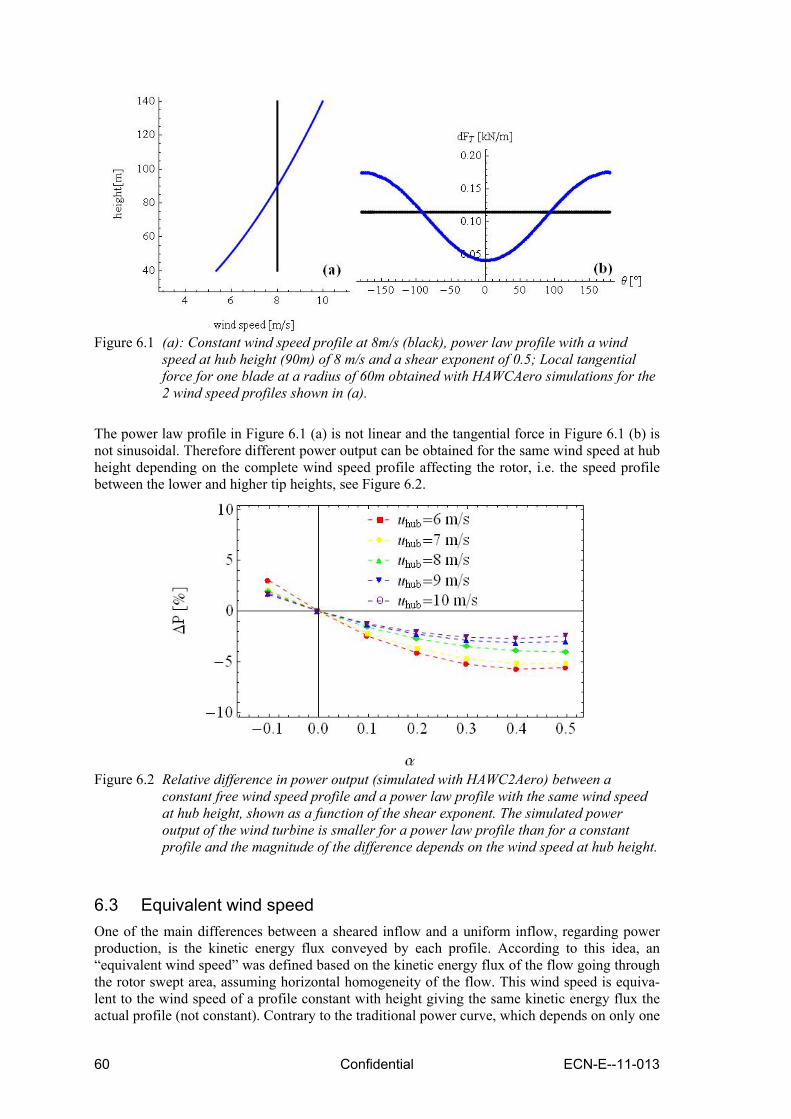
60 Confidential ECN-E--11-013
Figure 6.1 (a): Constant wind speed profile at 8m/s (black), power law profile with a wind
speed at hub height (90m) of 8 m/s and a shear exponent of 0.5; Local tangential force for one blade at a radius of 60m obtained with HAWCAero simulations for the 2 wind speed profiles shown in (a).
The power law profile in Figure 6.1 (a) is not linear and the tangential force in Figure 6.1 (b) is not sinusoidal. Therefore different power output can be obtained for the same wind speed at hub height depending on the complete wind speed profile affecting the rotor, i.e. the speed profile between the lower and higher tip heights, see Figure 6.2.
Figure 6.2 Relative difference in power output (simulated with HAWC2Aero) between a
constant free wind speed profile and a power law profile with the same wind speed at hub height, shown as a function of the shear exponent. The simulated power output of the wind turbine is smaller for a power law profile than for a constant profile and the magnitude of the difference depends on the wind speed at hub height.
6.3 Equivalent wind speed One of the main differences between a sheared inflow and a uniform inflow, regarding power production, is the kinetic energy flux conveyed by each profile. According to this idea, an “equivalent wind speed” was defined based on the kinetic energy flux of the flow going through the rotor swept area, assuming horizontal homogeneity of the flow. This wind speed is equiva-lent to the wind speed of a profile constant with height giving the same kinetic energy flux the actual profile (not constant). Contrary to the traditional power curve, which depends on only one

ECN-E--11-013 Confidential 61
wind speed (at hub height), the use of this equivalent wind speed results in a power curve ac-counting for the influence of shear.
This method was first tested with aerodynamic (BEM) simulations of a MW wind turbine sub-jected to various shears [2]. The use of the equivalent wind speed was found to reduce the scat-ter due to vertical shear in the power curve.
6.4 Experimental validation of the method The major challenge in the experimental application of the equivalent wind speed method is to characterize the speed profile in front of the wind turbine. As Lidars measure the wind speed at several heights, it enables us to measure the horizontal wind speed profile in front of the wind turbine rotor. Better than a hub height mast, with a Lidar, measurements can be taken up to the highest tip height, i.e. nor assumptions neither extrapolation are needed above hub height. A good approximation of the kinetic energy flux can thus be obtained.
A Lidar was installed in front of a MW wind turbine in order to measure the upcoming wind speed profile. The power curves scatter plot obtained with the equivalent wind speed derived directly from the Lidar measurements presented less scatter than the traditional power curve ob-tained with measurements at hub height only, see Figure 6.3. This method therefore results in a power curve which is less dependent on the shear than the current standard power curve. It is to be noted though that it is not completely independent of the shear as the power performance of the turbine does not depend only on the kinetic energy flux but also on the response of the tur-bine to various shear conditions.
Figure 6.3 Scatter (quantified as the normalized residuals) in the power curves obtained with
the wind speed at hub height only and the equivalent wind speed (derived from Lidar wind speed profile measurement). The use of the equivalent wind speed reduce decreases the scatter due to shear in the power curve.

62 Confidential ECN-E--11-013
6.5 Conclusions As it is less dependent of the shear, this power curve is more repeatable, i.e. nearly identical power curve can be obtained for various shear conditions, e.g. various seasons and/or various locations. Such a power curve not only facilitates the comparison of the performance of various turbines, but also improves the AEP prediction. Indeed the AEP prediction at a site potentially selected to build a wind farm is usually based on a power curve measured prior to the installa-tion of the turbines at another site.
Furthermore, the reduction of scatter in the power curve results in the decrease of the category uncertainty in power curve measurement (according to IEC 61400-12-1 definitions). However the combined uncertainty in power curve measurement was not reduced because the reduction in category A uncertainty was counterbalanced by an increase in the category B wind speed measurement uncertainty. This is due to the fact that the wind speed was measured by a Lidar, of which, as an instrument recently introduced to wind energy, the measurement uncertainty was defined relative to the uncertainty of cup anemometers, and also that the category B uncer-tainty due to wind shear in IEC 61400-12-1 is not taken into account.
6.6 References
[1] IEC 61400-12-1 Power performance measurements of electricity producing wind turbines, Ed.2 , 2005
[2] Wagner R., Antoniou I., Pedersen S.M., Courtney M.S. and H.E. Jørgensen, 2009: The in-fluence of the wind speed profile on wind turbine performance measurements, Wind Ener-gy, 12:348-362.
[3] Elliott DL and Cadogan JB, Effect of wind shear and turbulence on wind turbines power curve, EWEC 1990
[4] Sumner J and Masson M, Influence of atmospheric stability on wind turbine power per-formance curves, Journal of solar energy engineering, 128:531—538,2006

ECN-E--11-013 Confidential 63
7. Influence of offshore wakes on power performance at large distances
Jan Willem Wagenaar
7.1 Introduction The issue of turbulence intensity or rather added turbulence intensity due to offshore wind tur-bines is addressed. The turbulence intensity is measured in the wake of the turbine. By making proper wind direction selections, various turbines can be addressed and therefore the turbulence intensity can be measured at various distances from a wind turbine. These turbulence intensities are not only considered in single wakes, but also in multiple wakes. Studying increased turbu-lence intensity levels is done by considering data where turbines are on or off. The relevance to power performance is that the standard IEC 61400-12-1 [1] states that objects are considered to be disturbing up to 20 diameters (20D). By measuring and analysing the turbu-lence intensity it can be studied to which distances added turbulence is still present. The pres-ence of added turbulence of one turbine to another influences the power performance of the lat-ter turbine. The wind farm under consideration is the OWEZ wind farm. It consists of 36 Vestas V90 tur-bines, having a rotor diameter (D) of 90m and a rated power of 3MW, and a meteo mast meas-uring the wind speed and direction at least at hub height. More details can be found in [2]. A lay-out of the farm is given in Figure 7.1. The coloured lines indicate single and multiple wake directions as seen from the meteo mast.
Figure 7.1 OWEZ lay-out with wake indication.

64 Confidential ECN-E--11-013
7.2 Data selection The meteo mast was installed in the summer of 2005 [3] and the turbines were erected in the last part of 2006. For the latter activities the possible influence on the wind measurements are exam-ined in [4]. Those measurement points that were found to be effected are removed from the dataset. In the same period, i.e. the last half year of 2006 test runs of the turbines took place. Because those dates could not be retrieved, all data points that were taken in that period and for which the wind was from the disturbing sector are left out. All other obviously wrong data points are removed from the set as well. For all three heights at the meteo mast a wind speed and a wind direction has been defined for which the mast influences are minimised (see [5]). Those are called the “true” wind speed and “true” wind direction, respectively. In the remainder of this document the wind speed refers to the “true” wind speed at 70m (hub height) and the wind direction refers to the “true” wind direc-tion at 70m as measured by the meteo mast. The turbulence intensity is defined as
70
70
UTI Uσ= , ( 7.8 )
Where U70 is the 10 minute mean value of the (true) wind speed and σU70 is the standard devia-tion. For most analyses wind speeds are selected above 4m/s; these selections are however ex-plicitly mentioned. In the remainder of this chapter data will be selected based on turbines being “on” or “off”; a turbine is “on” when it is producing power below rated (0<P<3000 kW) and “off” when it is not producing power. For all other turbines, i.e. for those turbines that are not explicitly mentioned in the text regarding data selection, it is not know whether these turbines are producing power or not. For some data points these unmentioned turbines are on, for others they are off. Those data selections that are used, but are not listed above, are explicitly mentioned in text.
7.3 Null measurements Before investigating the turbulence in the wake of the turbines, it is interesting to see what the turbulence level is, when there are no power producing turbines. This can be considered as a null measurement. Figure 7.2 shows the turbulence intensity as function of the wind direction. The data considered are data points taken before the turbines became active, i.e. before the 1st of January 2007. The upper plot shows scatter data and the lower plot shows the binned values. Here, a bin size of 2.5 degrees is chosen and wind speeds above 4m/s are considered. The uncertainty bars are the standard uncertainty of each bin mean. The turbulence intensity is lowest around 150 degrees with a value of about 5%. The highest values are found around 350 degrees, which are about 7.5%. Similar figures are presented in [5] where the half-yearly data are presented.

ECN-E--11-013 Confidential 65
Figure 7.2 Turbulence intensity as function of wind direction when there are no power
producing turbines.
7.4 Single Wakes
7.4.1 Turbulence intensity: Wind speed dependency To see to what extend the turbulence intensity depends on the wind speed, turbine T9 is consid-ered. This turbine is located at a distance of 916m (=10.2D) from the meteo mast and at an angle of 340 degrees. A wind direction window of 5 degrees is chosen. With respect to the meteo mast T9 produces a single wake, when it is active. Figure 7.3 shows the turbulence intensity as function of the wind speed, where wind speed re-fers to the wind speed in the wake. The upper plot shows the scatter data and the lower plot the binned values, where a bin size of 1m/s is chosen. Distinction is made whether turbines are on or off. For the scatter data no wind speed selection is made, however a few extreme data points are not shown, i.e. are not within the shown window of TI and wind speed. For the binned val-ues in the lower plot, only wind speeds between 4m/s and 16m/s are considered. The uncertainty bars are the standard uncertainty of the bin mean. When the turbines are on, it is seen in the lower plot of Figure 7.3 that the turbulence intensity decreases with increasing wind speed. From about 9.5m/s to 15.5m/s the turbulence intensity drops from about 11.5% to 8.5%.
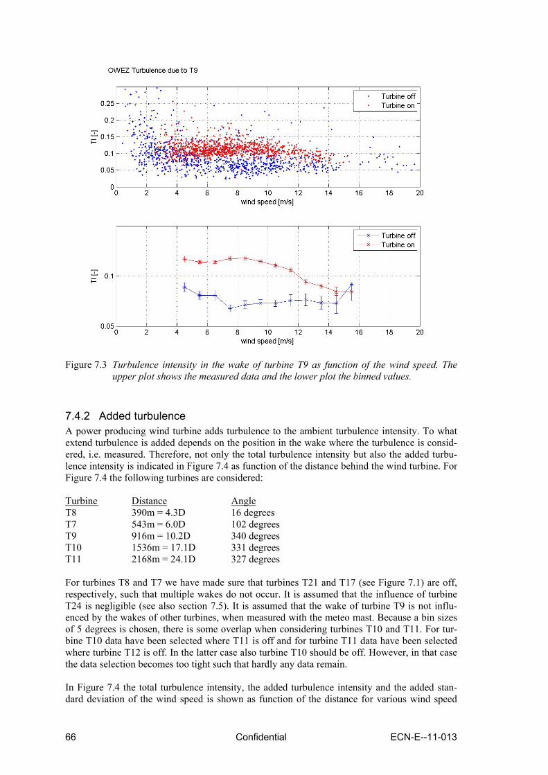
66 Confidential ECN-E--11-013
Figure 7.3 Turbulence intensity in the wake of turbine T9 as function of the wind speed. The
upper plot shows the measured data and the lower plot the binned values.
7.4.2 Added turbulence A power producing wind turbine adds turbulence to the ambient turbulence intensity. To what extend turbulence is added depends on the position in the wake where the turbulence is consid-ered, i.e. measured. Therefore, not only the total turbulence intensity but also the added turbu-lence intensity is indicated in Figure 7.4 as function of the distance behind the wind turbine. For Figure 7.4 the following turbines are considered: Turbine Distance Angle T8 390m = 4.3D 16 degrees T7 543m = 6.0D 102 degrees T9 916m = 10.2D 340 degrees T10 1536m = 17.1D 331 degrees T11 2168m = 24.1D 327 degrees For turbines T8 and T7 we have made sure that turbines T21 and T17 (see Figure 7.1) are off, respectively, such that multiple wakes do not occur. It is assumed that the influence of turbine T24 is negligible (see also section 7.5). It is assumed that the wake of turbine T9 is not influ-enced by the wakes of other turbines, when measured with the meteo mast. Because a bin sizes of 5 degrees is chosen, there is some overlap when considering turbines T10 and T11. For tur-bine T10 data have been selected where T11 is off and for turbine T11 data have been selected where turbine T12 is off. In the latter case also turbine T10 should be off. However, in that case the data selection becomes too tight such that hardly any data remain. In Figure 7.4 the total turbulence intensity, the added turbulence intensity and the added stan-dard deviation of the wind speed is shown as function of the distance for various wind speed

ECN-E--11-013 Confidential 67
classes (and all wind speeds). Here, a wind speed bin of 1m/s is chosen and a wind direction window of 5 degrees. The following definitions are used:
022
0
σσσ −=
−=
totaladded
totaladded TITITI, ( 9.2 )
where TIadded, TItotal and TI0 indicate the added, the total and the ambient turbulence intensity. This also applies for the standard deviation of the wind speed σ. It is clearly seen that the added turbulence intensity and added standard deviation of the wind speed in a single wake decreases with increasing distance. The level of turbulence intensity de-pends on the wind speed. More importantly, we see that the presence of added turbulence intensity at and beyond 20D. It has vanished at about 25D (=2250m).

68 Confidential ECN-E--11-013
Figure 7.4 Total and added turbulence intensity (upper and middle plot) as function of
distance. The lower plot shows the added standard deviation of the wind speed as function of distance. The blue, red, green and black curves indicate wind speeds of 8m/s, 10m/s, 12m/s and all wind speeds, respectively.
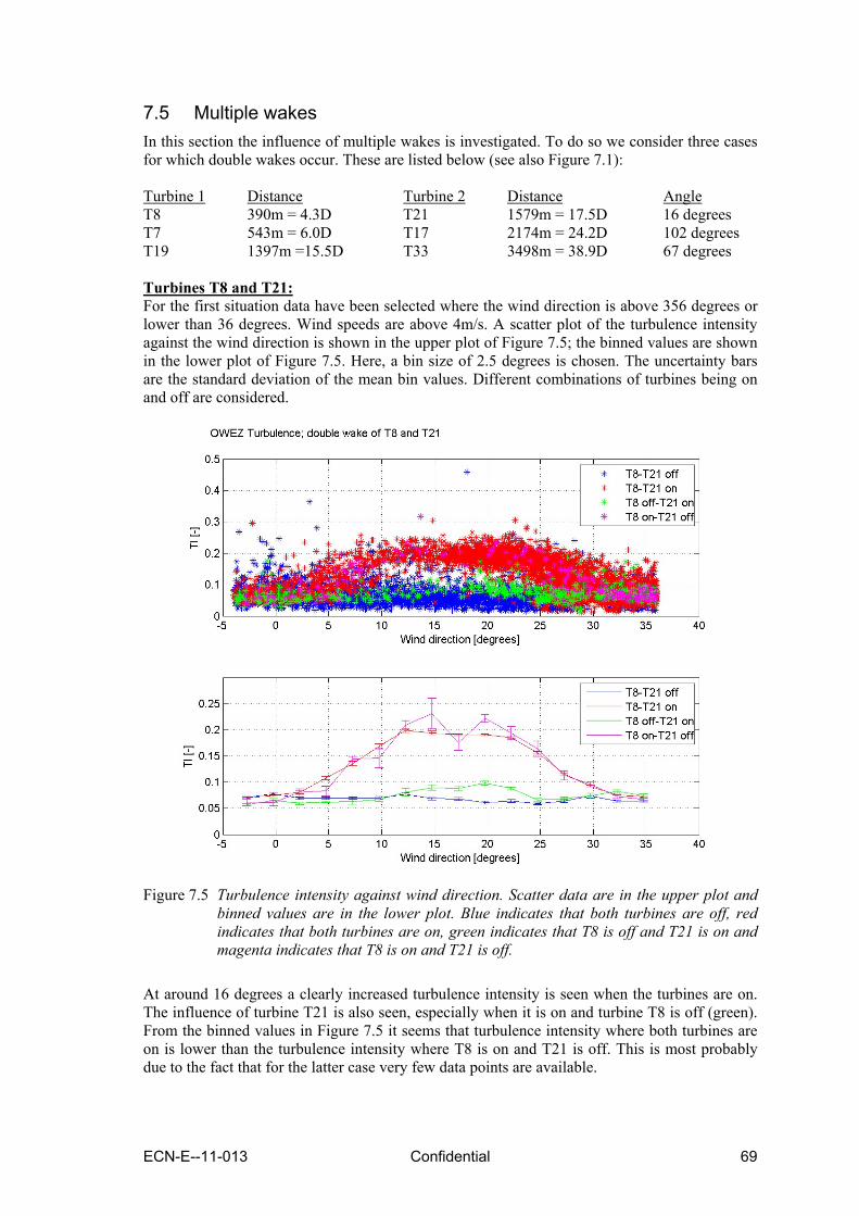
ECN-E--11-013 Confidential 69
7.5 Multiple wakes In this section the influence of multiple wakes is investigated. To do so we consider three cases for which double wakes occur. These are listed below (see also Figure 7.1): Turbine 1 Distance Turbine 2 Distance Angle T8 390m = 4.3D T21 1579m = 17.5D 16 degrees T7 543m = 6.0D T17 2174m = 24.2D 102 degrees T19 1397m =15.5D T33 3498m = 38.9D 67 degrees Turbines T8 and T21: For the first situation data have been selected where the wind direction is above 356 degrees or lower than 36 degrees. Wind speeds are above 4m/s. A scatter plot of the turbulence intensity against the wind direction is shown in the upper plot of Figure 7.5; the binned values are shown in the lower plot of Figure 7.5. Here, a bin size of 2.5 degrees is chosen. The uncertainty bars are the standard deviation of the mean bin values. Different combinations of turbines being on and off are considered.
Figure 7.5 Turbulence intensity against wind direction. Scatter data are in the upper plot and
binned values are in the lower plot. Blue indicates that both turbines are off, red indicates that both turbines are on, green indicates that T8 is off and T21 is on and magenta indicates that T8 is on and T21 is off.
At around 16 degrees a clearly increased turbulence intensity is seen when the turbines are on. The influence of turbine T21 is also seen, especially when it is on and turbine T8 is off (green). From the binned values in Figure 7.5 it seems that turbulence intensity where both turbines are on is lower than the turbulence intensity where T8 is on and T21 is off. This is most probably due to the fact that for the latter case very few data points are available.

70 Confidential ECN-E--11-013
Furthermore, we note that wind speed dependency is present, but it does not influence the pre-sented results significantly. Turbines T7 and T17: For turbines T7 and T17 a similar situation applies. Here, data have been chosen where the wind direction is between 92 degrees and 112 degrees and wind speeds above 4m/s. The upper plot of Figure 7.6 shows the scatter data and the lower plot the binned values where a bin size of 2.5 degrees is chosen. The uncertainty bars are the standard deviation of the mean bin values. The different colours stand for different combinations of turbines being on and off.
Figure 7.6 Turbulence intensity against wind direction. Scatter data are in the upper plot and
binned values are in the lower plot. Blue indicates that both turbines are off, red indicates that both turbines are on, green indicates that T7 is off and T17 is on and magenta indicates that T7 is on and T17 is off.
An increased turbulence intensity is present when the turbines are on. Furthermore, the influ-ence of turbine T17 on the turbulence intensity measured at the meteo mast is clearly seen, both when turbine T7 is on and off. When turbine T7 is off we see an increase of turbulence intensity when T17 is turned on and vice versa when turbine T7 is on an decrease in turbulence intensity is seen when turbine T17 is turned off. According to IEC 61400-12-1 [1] a turbine at a distance further than 20D is not considered as a disturbance to the wind measurements. From Figure 7.6 it is clearly seen that turbine T17, being at a distance of 24.2D, is influencing the wind measurements in the sense that the turbulence in-tensity is affected.

ECN-E--11-013 Confidential 71
Turbines T19 and T33: To further investigate this point, the turbines T19 (15.5D) and T33 (38.9D) are considered. Wind directions are chosen between 55 and 57, where binning is applied with a bin size of 2.5 degrees. Wind speeds are all above 4m/s. For these conditions the turbulence intensity is given in Figure 7.7 as function of the wind direction. The upper plot shows the scatter data and the lower plot the binned values, where the uncertainty bars are the standard deviation of the mean bin values.
Figure 7.7 Turbulence intensity against wind direction. Scatter data are in the upper plot and
binned values are in the lower plot. Blue indicates that both turbines are off, red indicates that both turbines are on, green indicates that T19 is off and T33 is on and magenta indicates that T19 is on and T33 is off.
As in the previous examples (Figure 7.5 and Figure 7.6) an increased turbulence intensity is seen when the turbines are on. The influence of the second turbine, i.e. the turbine in line that is furthest away, in this case turbine T33, is not as clear as in the previous examples. This is ex-pected because the distance of this second turbine is very large (38.9D). The effect of turbine T33 is best seen when it is on and turbine T19 is off (green). The lower plot shows an increase of at most 1% when turbine T33 is turned on. Triple wakes: As can be seen from Figure 7.1 a triple wake situation can be identified. It involves the turbines T7, T17 and T24. Here, turbine T24 is at a distance of 3638m or 40.4D. Unfortunately, too few data points are available to make a proper analysis.

72 Confidential ECN-E--11-013
7.6 Conclusions The main conclusions are summarized as follows:
• The total turbulence intensity in a single wake decreases with increasing wind speed. From about 9.5m/s to 15.5m/s it drops from about 11.5% to 8.5%.
• It is clearly seen that the added turbulence intensity and added standard deviation of the wind speed in a single wake decreases with increasing distance. The level of turbulence intensity depends on the wind speed. More importantly, added turbulence intensity is present at and beyond 20D. It has vanished at about 25D (=2250m).
• In double wake measurements including T7 and T17 the effect of the second turbine (T17), being at a distance of 24.2D, on the turbulence intensity is clearly seen.
• In double wake measurements including T19 and T33 the effect of the second turbine (T33, distance is 38.9D) is not as clear as in the previous example. When turbine T33 is on and turbine T19 is off the increase in turbulence intensity is at most 1%.
7.7 References [1] IEC 61400-12-1:2005(E), Power performance measurements of electricity producing
wind turbines [2] H.J. Kouwenhoven, User manual data files meteorological mast NoordzeeWind, NZW-
16-S-4-R03, October 2007 [3] J.W. Wagenaar, P.J. Eecen, Measurements of Wind, Wave and Currents at the Offshore
Wind Farm Egmond aan Zee, ECN-E--09-015 [4] A. Curvers, P.A. van der Werff, OWEZ WIND FARM EFFICIENCY, ECN-E--08-092 [5] P.J. Eecen, L.A.H. Machielse and A.P.W.M. Curvers, Meteorological Measurements
OWEZ, Half year report 01-07-2005 – 31-12-2005, ECN-E--07-073
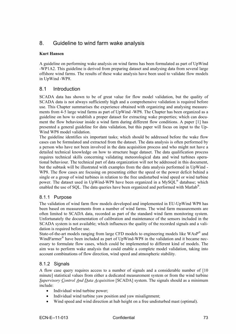
ECN-E--11-013 Confidential 73
8. Guideline to wind farm wake analysis
Kurt Hansen A guideline on performing wake analysis on wind farms has been formulated as part of UpWind -WP1A2. This guideline is derived from preparing dataset and analysing data from several large offshore wind farms. The results of these wake analysis have been used to validate flow models in UpWind -WP8.
8.1 Introduction SCADA data has shown to be of great value for flow model validation, but the quality of SCADA data is not always sufficiently high and a comprehensive validation is required before use. This Chapter summarises the experience obtained with organizing and analysing measure-ments from 4-5 large wind farms as part of UpWind -WP8. The Chapter has been organized as a guideline on how to establish a proper dataset for extracting wake properties; which can docu-ment the flow behaviour inside a wind farm during different flow conditions. A paper [1] has presented a general guideline for data validation, but this paper will focus on input to the Up-Wind WP8 model validation. The guideline identifies six important tasks; which should be addressed before the wake flow cases can be formulated and extracted from the dataset. The data analysis is often performed by a person who have not been involved in the data acquisition process and who might not have a detailed technical knowledge on how to structure huge dataset. The data qualification process requires technical skills concerning validating meteorological data and wind turbines opera-tional behaviour. The technical part of data organization will not be addressed in this document, but the subtask will be illustrated with examples from the data analysis performed in UpWind -WP8. The flow cases are focusing on presenting either the speed or the power deficit behind a single or a group of wind turbines in relation to the free undisturbed wind speed or wind turbine power. The dataset used in UpWind-WP8 have been organized in a MySQL® database; which enabled the use of SQL. The data queries have been organized and performed with Matlab®.
8.1.1 Purpose The validation of wind farm flow models developed and implemented in EU-UpWind WP8 has been based on measurements from a number of wind farms. The wind farm measurements are often limited to SCADA data, recorded as part of the standard wind farm monitoring system. Unfortunately the documentation of calibration and maintenance of the sensors included in the SCADA system is not available; which influences the quality of the recorded signals and a vali-dation is required before use. State-of-the-art models ranging from large CFD models to engineering models like WAsP® and WindFarmer® have been included as part of UpWind-WP8 in the validation and it became nec-essary to formulate flow cases, which could be implemented to different kind of models. The aim was to perform wake analysis that could enable a complete model validation, taking into account combinations of flow direction, wind speed and atmospheric stability.
8.1.2 Signals A flow case query requires access to a number of signals and a considerable number of [10 minute] statistical values from either a dedicated measurement system or from the wind turbine Supervisory Control And Data Acquisition [SCADA] system. The signals should as a minimum include:
• Individual wind turbine power; • Individual wind turbine yaw position and yaw misalignment; • Wind speed and wind direction at hub height on a free undisturbed mast (optimal).

74 Confidential ECN-E--11-013
All statistical values should be screened to: • Identify records with turbines of line; • Identify records with reduced power settings; • Identify wind farm offline situations; • Identify site specific deviations e.g. turbine size, hub height, regulation type and terrain.
8.1.3 Definitions Some basic definitions have been adapted during the flow validation procedure. When analysing flows inside wind farms, the input refers to wind speed or [wind turbine] power and the output is expressed as the ratio between output and input values or as a deficit. The following defini-tions have been used:
Speed ratio: ηs = Ufree / Uwake Power ratio: ηp = Powerfree / Powerwake Speed deficit: ηsd = 1-Ufree / Uwake Power deficit: ηpd = 1-Powerfree / Powerwake Turbine spacing, unit= [Rotor] diameter
The deficit is presented according to the [ambient] flow conditions as function of distance be-tween the [wake] object wind turbine and the wake generating turbine as function of flow direc-tion. The power deficit distribution is illustrated in 2 different presentations below: Figure 8.1; illustrates the power deficit distribution - as function of the normalized inflow direc-tion where each circle represents the mean power deficit for a five degree flow sector between two turbines. The distribution is fitted with a Gaussian expression and reveals a mean wake ex-pansion of 28°. The deficit distribution represents all atmospheric conditions in the wind speed interval 7 – 9 m/s for 7D spacing in the Horns Rev wind farm.
Figure 8.1: Example of power deficit as function of normalized wind direction between two
turbines with 7D spacing.

ECN-E--11-013 Confidential 75
Figure 8.2; shows the mean power deficit downstream, along rows of turbines with 7D spacing for 8 m/s wind speed and a 5 degree flow sector. The figure illustrates how the main part of deficit 30-40% occurs between the 1th and the 2th turbine. Adding some additional turbines to the row, only increases the power deficit with 10% - with reference to the first turbine. The power deficit level and shape highly depends on the wind speed, flow direction and the atmospheric stability.
Figure 8.2: Averaged deficit along 6 rows of turbines with reference to wt07 for a 5 degree flow
sector.
8.2 Data preparation Before a wake analysis can be performed it is necessary to establish a high quality dataset to give confidence to the results. The recommended number of reliable observations is at least 30-60 minutes of good measurements for each flow case, which can be difficult to obtain after the data filtering. This requires a large number of “raw” observations corresponding to at least 1- 2 years of wind farm operation. The necessary subtasks for qualifying a dataset to wake analysis are:
1. Data organization and synchronization; 2. Data qualification; 3. Wind farm layout; 4. Calculation of derived parameters; 5. Identification of descriptors and flow cases; 6. Define data filter criteria;
It is important to address all the tasks listed above; otherwise the data query will suffer from large scatter or a lack of observations.
8.3 Signals, organization and synchronization The required data for wake flow analysis should include both primary signals like individual power values, wind speed and wind direction at hub height. Furthermore a lot of secondary sig-nals e.g. individual values for yaw position, nacelle wind speed, pitch angle and rotor speed. The secondary values are important for validating the quality of the primary signal quality and also for validating the operational behaviour of the wind turbine. The signal statistics should in-clude mean, standard deviation, minimum and maximum values both for primary and secondary signals.

76 Confidential ECN-E--11-013
Table 8.1: Required SCADA signals, used to
qualify the wake flow properties in a wind farm Number Signal Importance 1 Electric Power from all wind turbines High 2 Wind speed from undisturbed mast(s) 2 High 3 Wind direction at hub height High 4 Yaw position from all individual turbines3 High 5 Nacelle wind speed from all wind turbines Medium 6 Rotor speed from all turbines4 Medium 7 Pitch angle from all turbines Medium 8 Temperatures Medium
The data organization should be appropriate to avoid additional scaling or calibration during queries. Furthermore it should be possible to perform queries with a number of constraints. The data transfers include many GB of data, stored in huge compressed [ASCII] files and a data conversion to a robust format is required. Such format can be a database or a software dedicated format. A database solution enables the use of efficient tools based on Structured Query Lan-guage [SQL]. The wind farm statistics are available from different sources as the Supervisory Control And Data Acquisition [SCADA] system or stand-alone [meteorological] logger systems. It is ex-tremely important to facilitate a robust synchronization of the different sources of measure-ments, because system clocks can be unstable for stand-alone systems. The quality of the syn-chronization should be within 1 minute; which has to be checked throughout the whole measur-ing period.
8.3.1 Wind farm layout The exact knowledge of the wind farm layout is essential, both during the data qualification and for the wake analysis. The wind turbine coordinates are available as geographical coordinates, but often it is more appropriate to use the rotor diameter as plotting unit demonstrated in Figure 8.3. This figure presents the layout of an [offshore] wind farm with 80 turbines and the position of three masts. It is important to identify free inflow sectors both for the masts observations and for wind turbines. Figure 8.4 identifies the three principal flow directions corresponding to 7D, 9.4D and 10.4 D spacing at the NW corner of the wind farm. This information is essential when validating the signal quality. The wind turbine coordinates are used to identify the wake gener-ating turbines, according to the inflow sector. Wind farms located in complex terrain are often installed in irregular shapes optimized to the landscape or dominants flow sectors. It can be difficult to determine a unique inflow reference due to the complexity of the terrain and the lack of undisturbed masts. This is shown in Figure 8.5, where the masts are located inside the wind farm or behind the wind farms compared to the dominant flow direction.
2 This will require several masts, but in case such signal is not available, it is necessary to use the power values to determine the inflow conditions. 3 This signal is equal to nacelle position, and can be a substitute to the wind direction signal. 4 The rotor speed is important for validating the operational behavior of dual or variable speed turbines.

ECN-E--11-013 Confidential 77
Figure 8.3: Layout of the Horns rev wind farm, unit=rotor diameter (=80m).
Figure 8.4: Main flow directions and principal spacing distances at Horns Rev wind farm.

78 Confidential ECN-E--11-013
Figure 8.5: Example of a wind farm installed in a complex terrain with a dominant flow
direction.
8.3.2 Data qualification Before use, all data need to be quality checked while the data has been moved to another media using a transfer protocol. Furthermore data is not necessarily checked during the operational phase due to lack of time or skilled personnel. It is important to identify and exclude erroneous observations instead of using modified observations and exclusion might be implemented using a quality number as defined in [2]. Below is a list of potential error sources related to the signals in Table 8.1, which need to be verified. Power signals can: • include outliers, which can influence the analysis; • include periods where the turbine is in transition mode like start, stop or emergency stop se-
quence; • be limited due to power de-regulation. The main part of deviating power observations can be identified through scatter plot of the power as function of nacelle wind speed. It can even be necessary to establish a correlation be-tween the official power curve and the mean power curve based on the nacelle wind speed as shown in Figure 8.6. A scatter plot of the power value as function of the nacelle wind speed can be used to identify outliers if there is a lack of undisturbed wind speed observations, especially for wind turbines located in a wind farm. A qualifying scatter plot is shown in Figure 8.7 including a disqualifica-tion line and circle. The level of the disqualification line depend a.o. on the wind turbine control and the local turbulence intensity variation.

ECN-E--11-013 Confidential 79
Figure 8.6: Official power and thrust coefficient curve for VESTAS V80.
Figure 8.7: Example of qualification of power values, all observations below the red line and
inside the red circle are marked as outliers and disqualified.

80 Confidential ECN-E--11-013
If the power values contain a high degree of scatter it is necessary to include an “acceptance” band for each wind speed interval with reference to the standard deviation of the power. Wind speed at hub height • could be checked for correlation with other heights; • Could be checked for occurrence of stationarity, spikes and drop-outs through scatter plots. The signal correlation is a robust method to identify data outliers and scatter plots of turbulence can be used but to identify signal stationarity. Unfortunately it is impossible to verify the in-strument calibration due to lack of documentation. Wind direction at hub height • could be checked for correlation with other heights; • Could be checked for occurrence of stationarity through scatter plots. Yaw position of wind turbine The wind turbine yaw position offset is often not correct or calibrated and it is necessary to per-form a data analysis to determine this offset. A correlation against the wind speed direction is sufficient for a free wind sector; otherwise the signal could be verified in sectors with an ex-pected power deficit along a line of turbines, as shown in Figure 8.8. It is sufficient to validate the yaw position for 3 – 4 reference turbines; which can represent the flows from different direc-tion into the wind farm, if the number of masts is limited. The yaw position offset can change during the measuring period and this also need to be verified.
Figure 8.8: Determination of yaw position offset from Horns rev, wt02.
Each observation in Figure 8.8 is determined with a moving average technique using a window of 5 degrees. The moving window technique reduces the deficit scatter and is a robust technique to extract information from small datasets.
8.3.3 Derived parameters The wind farm dataset does not always include the sufficient signals for wake analysis. This section identifies important signals, which should be included as constraints in the wake analy-sis. Free wind direction The wind direction signal is extremely important, while the flow deficit highly depends on the flow direction (Figure 8.8) and the spacing between the wind turbines. With a lack of direction measurements it is necessary to establish an artificial wind direction based yaw positions from 2-4 wind turbines to cover the whole wind rose. NOTE: The artificial signal is only valid for grid connected wind turbines, while the wind turbine yaw position could misbehave when the turbine is idling or stopped.

ECN-E--11-013 Confidential 81
Monin-Obukhov length, L. The M-O length can be derived either from sonic measurements or from a combination of the temperature and the wind speed gradient. To determine a robust M-O lengths in onshore and complex terrain sites, it is important to select proper observation heights and it is recommended to consult the literature on this topic. Atmospheric stability classification The offshore stability classification can be based on the Monin-Obukhov length L, as listed in Table 8.2
Table 8.2: Definition of stability classes based on length, L (m). Class Obukhov length [m] Atmosperic stability classcL=-3 -100 ≤ L ≤ -50 Very unstable (vu)cL=-2 -200 ≤ L ≤ -100 Unstable (u)cL=-1 -500 ≤ L ≤ -200 Near unstable (nu)cL=0 |L|>500 Neutral (n)cL=1 200 ≤ L ≤ 500 Near stable (ns)cL=2 50 ≤ L ≤ 200 Stable (s)cL=3 10 ≤ L ≤ 50 Very stable (vs)
The stability classification for Horns Rev has been based on the Bulk-Ri number with success - as demonstrated in [3,4]. The speed measurements from 15 m amsl (recorded below tip-bottom height) seem to be applicable in combination with the temperature difference between air and water. The robustness of this classification has been documented in [4] and an example from Horns Rev has been demonstrated in Figure 8.9.
Figure 8.9: Example of averaged turbulence intensity for different
stability classifications, measured at Horns Rev offshore wind farm, Denmark.

82 Confidential ECN-E--11-013
8.3.4 Identifications of descriptors and flow cases The two most important descriptors for analysing the flow inside a wind farm is 1) the undis-turbed wind speed and 2) wind direction at hub height measured outside the wind farm. Unfor-tunately such observations are not always available and another option is to use recordings from a upwind turbine, e.g. power values and yaw position as indicated in Figure 8.11. The power range is selected according to the official power curve, Figure 8.6, for a given wind speed interval, but this method requires a signal validation as described in section 4.3 before the analysis can be performed. The inflow sector is limited with reference to the [upwind] free wind turbine yaw position as illustrated in Figure 8.12. Using the wind turbine yaw position increases the directional uncer-tainty, while the wind turbine yaw misalignment averaging procedure is not documented, but a |yaw misalignment| > 0 can be expected5. Many observations are required to reduce the scatter in the measurements compared to wind vane signals. Other descriptors can be the ambient turbulence intensity and/or the stability classification as listed in the section 4.4. The flow case is defined together with the users who are validating flow models; which is could either be the code developers or the end-users who need the flow model performance. The flow cases are defined in steps; ranging from simple [flow] cases to very complicate [flow] cases and a list with increasing complexity is given in Figure 8.10:
Figure 8.10: Definition of flow cases with increasing complexity. i) Flow within a limited sector, along a line of wind turbine; ii) Flow within a limited sector, along a line of wind turbines and a limited wind speed in-
terval; iii) Flow within a limited sector, along a line of wind turbines, a limited wind speed interval
and a stability class. The simple flow case i) is applicable for a limited number of observations and depends only on the selected sector size. Increasing complexity requires much more observations and flow cases from class iii) can only be fulfilled with a limited number of combinations of wind speed, flow sectors and stability classes. The number of flow cases derived from class iii) could include 18 flow sectors x 12 wind speeds interval x 7 stability classes – in total 1512 flow cases6. Such amount of cases requires a proper verification and planning before the queries can be performed. The size of the flow sector should be applicable for the flow model verification and may vary between 5 and 30 degrees.
5 Caused by a hysteresis, in the yaw misalignment. 6 Many flow cases can be eliminated due to symmetry, depending on the wind farm layout and inflow complexity.

ECN-E--11-013 Confidential 83
Figure 8.11: Wind farm inflow conditions
Figure 8.12: Definition of 30 degrees flow sector along a row of turbines.
I
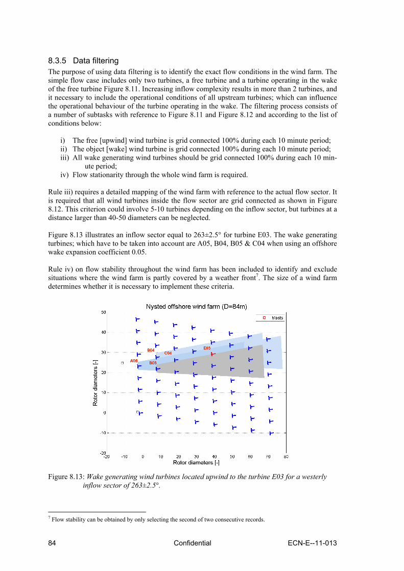
84 Confidential ECN-E--11-013
8.3.5 Data filtering The purpose of using data filtering is to identify the exact flow conditions in the wind farm. The simple flow case includes only two turbines, a free turbine and a turbine operating in the wake of the free turbine Figure 8.11. Increasing inflow complexity results in more than 2 turbines, and it necessary to include the operational conditions of all upstream turbines; which can influence the operational behaviour of the turbine operating in the wake. The filtering process consists of a number of subtasks with reference to Figure 8.11 and Figure 8.12 and according to the list of conditions below:
i) The free [upwind] wind turbine is grid connected 100% during each 10 minute period; ii) The object [wake] wind turbine is grid connected 100% during each 10 minute period; iii) All wake generating wind turbines should be grid connected 100% during each 10 min-
ute period; iv) Flow stationarity through the whole wind farm is required.
Rule iii) requires a detailed mapping of the wind farm with reference to the actual flow sector. It is required that all wind turbines inside the flow sector are grid connected as shown in Figure 8.12. This criterion could involve 5-10 turbines depending on the inflow sector, but turbines at a distance larger than 40-50 diameters can be neglected. Figure 8.13 illustrates an inflow sector equal to 263±2.5° for turbine E03. The wake generating turbines; which have to be taken into account are A05, B04, B05 & C04 when using an offshore wake expansion coefficient 0.05. Rule iv) on flow stability throughout the wind farm has been included to identify and exclude situations where the wind farm is partly covered by a weather front7. The size of a wind farm determines whether it is necessary to implement these criteria.
Figure 8.13: Wake generating wind turbines located upwind to the turbine E03 for a westerly
inflow sector of 263±2.5°.
7 Flow stability can be obtained by only selecting the second of two consecutive records.

ECN-E--11-013 Confidential 85
8.4 Data query and wake analysis The complexity of data query depends on the amount of available turbines ranging from 1) small wind farms with 10 - 40 turbines distributed in irregular patterns (complex terrain and complex inflow conditions) and low availability; to 2) large wind farms consisting of 30 – 100 wind turbines and requires more than 1 complete year of operation distributed in regular pat-terns (offshore and regular inflow conditions). Both types of wind farms or a combination can be analysed; but wind farms situated in a complex terrain is a big challenge due to the complex inflow conditions and even varying hub heights caused by the topography. Such analysis re-quires more than 1 year of observations to establish a robust estimate of the power deficit distri-butions. The wake analysis can be formulated according to the complexity of the flow conditions and the purpose: i) Deficit for pairs of turbines as function of wind direction; ii) Deficit for pairs of turbines with different spacing; iii) Maximum deficit as function of turbulence intensity and spacing; iv) Deficit along rows of turbines; v) Deficit for partly covered turbines as function of flow direction; vi) Deficit variations at different atmospheric conditions; vii) Park efficiency. These analyses require a well-organized and quality controlled dataset according to the guide-lines given in the previous section.
i) Deficit for a pair of turbines. This basic query requires a pair of [identical] turbines with spacing between 2-10D. The pur-pose of this analysis is to determine the deficit distribution a function of wind direction - as il-lustrated in Figure 8.1. Refined analysis can reveal the dependence due to wind speed level, ro-tor speed, pitch angle or turbulence intensity, because the angular deficit distribution depends on the actual operational turbine condition. ii) Deficit for a pair of turbines with different spacing. The deficit distribution for some distinct spacing can be derived from a group of turbines lo-cated in a wind farm. With turbines arranged in an ordinary grid; this enables at a number of spacing to be validated when taking into account the diagonals directions. Figure 8.4 defines three distinct spacing 7D, 9.4D and 10.4D for the Horns Rev wind farm. iii) Maximum deficit as function of turbulence intensity and spacing. The maximum deficit is determined for a narrow flow sector as function of turbulence intensity and spacing as shown in Figure 8.14. The flow sector size depends on the number of available observations, but increasing the flow sector decreases the maximum deficit value. Figure 8.14 illustrates a clear correlation between deficit, turbulence intensity and spacing. This query can furthermore be applied for more than two turbines and will then result in a multiple wake defi-cits estimate.
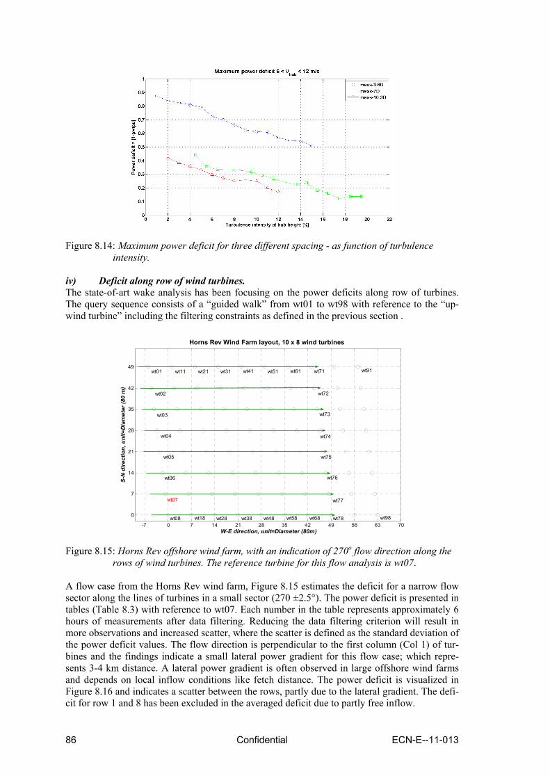
86 Confidential ECN-E--11-013
Figure 8.14: Maximum power deficit for three different spacing - as function of turbulence
intensity. iv) Deficit along row of wind turbines. The state-of-art wake analysis has been focusing on the power deficits along row of turbines. The query sequence consists of a “guided walk” from wt01 to wt98 with reference to the “up-wind turbine” including the filtering constraints as defined in the previous section .
-7 0 7 14 21 28 35 42 49 56 63 70
0
7
14
21
28
35
42
49
W-E direction, unit=Diameter (80m)
S-N
dire
ctio
n, u
nit=
Dia
met
er (8
0 m
)
Horns Rev Wind Farm layout, 10 x 8 wind turbines
wt03
wt04
wt02
wt05
wt78
wt07
wt98
wt11 wt21 wt31 wt41 wt51 wt61 wt71wt01 wt91
wt18
wt76wt06
wt75
wt74
wt73
wt72
wt77
wt28 wt38 wt48 wt58 wt68wt08
Figure 8.15: Horns Rev offshore wind farm, with an indication of 270o flow direction along the
rows of wind turbines. The reference turbine for this flow analysis is wt07.
A flow case from the Horns Rev wind farm, Figure 8.15 estimates the deficit for a narrow flow sector along the lines of turbines in a small sector (270 ±2.5°). The power deficit is presented in tables (Table 8.3) with reference to wt07. Each number in the table represents approximately 6 hours of measurements after data filtering. Reducing the data filtering criterion will result in more observations and increased scatter, where the scatter is defined as the standard deviation of the power deficit values. The flow direction is perpendicular to the first column (Col 1) of tur-bines and the findings indicate a small lateral power gradient for this flow case; which repre-sents 3-4 km distance. A lateral power gradient is often observed in large offshore wind farms and depends on local inflow conditions like fetch distance. The power deficit is visualized in Figure 8.16 and indicates a scatter between the rows, partly due to the lateral gradient. The defi-cit for row 1 and 8 has been excluded in the averaged deficit due to partly free inflow.

ECN-E--11-013 Confidential 87
Table 8.3: Mean power deficit at Horn Rev for flow direction = 270±2.5° and Vhub=8±0.5m/s
Col 1 Col 2 Col 3 Col 4 Col 5 Col 6 Col 7 Col 8 Col 9 Col 10row 1 1.02 0.74 0.73 0.71 0.72 0.68 0.65 0.63 0.61 0.59row 2 1.01 0.72 0.71 0.69 0.65 0.65 0.63 0.58 0.57 0.57row 3 1.02 0.69 0.69 0.64 0.63 0.61 0.61 0.58 0.57 0.56row 4 1.02 0.69 0.67 0.65 0.63 0.61 0.57 0.59 0.58 0.57row 5 0.99 0.67 0.67 0.62 0.62 0.60 0.60 0.59 0.59 0.55row 6 1.01 0.64 0.64 0.60 0.60 0.59 0.58 0.58 0.55 0.54row 7 1.00 0.63 0.62 0.58 0.56 0.55 0.55 0.53 0.52 0.51row 8 0.99 0.64 0.63 0.61 0.60 0.58 0.60 0.61 0.63 0.62
Flow case 8: Power deficit [filters: wake & stationarity ]
The park efficiency is calculated with reference to wt07 to 66%. The inflow condition for this number is an inflow sector: 270±2.5° and a wind speed, Vhub = 8±0.5 m/s and the number has been calculated as the average of all individual wind turbine deficit numbers from in Table 8.3.
Figure 8.16: Horns Rev Flow Case 8, power deficit along wind turbine rows. v) Deficit of turbines operating partly in wakes. When the flow direction deviates from the line of turbines the turbines are operating partly in wake and a query process identical to case iv) can be used. The results are organized in tables’ analogue to the example given in Table 8.3. Figure 8.17 defines the inflow sector with turbines, operating partly in wake, divided in 5 degree sectors. The averaged power deficit curves are shown for in Figure 8.18 for 7 different sectors ranging from sector 255, 265, .., 285° and the curves clearly illustrates how the power deficit depends of the wake coverage. When the flow direction deviates from the turbine row direction a speed-up effect is visible on the outer row, because this row is partly facing the wind. This is illustrated in Figure 8.19 for an inflow deviation of 15°, compared to the direction of the row, and the power deficit is reduced considerably.

88 Confidential ECN-E--11-013
Figure 8.17: Example of wind farm flow sector analysis for Horns Rev wind farm.
Figure 8.18: Mean deficit for turbines operating partly in wake.
Figure 8.19: Power deficit at Horns Rev wind farm for Vhub=8 m/s, WDIR=285±2.5°.

ECN-E--11-013 Confidential 89
vi) Deficit sensitivity due to stability. Adding an additional constraint in terms of stability in the data query, reduces the number of available observations but reveals an important correlation between the deficit and the stability classification. To obtain a recent amount of data for this query, both the wind speed interval and flow sector has been increased considerably. The previous 1 m/s wind speed interval combined with 5 degree flow sectors requires a huge amount of data when including the stability con-straint. Large wind speed intervals results in averaged wind turbine operational conditions; which are difficult to interpret and evaluate afterwards. The power deficits distributed according to the classification are shown in Figure 8.20 and indicates a distinct correlation to the atmos-pheric stability.
Figure 8.20: Power deficit along rows of wind turbines for different atmospheric stability
conditions.
vii) Wind farm efficiency. The efficiency of the wind farm deviates from an isolated wind turbine due to the wake deficit as determined above. The determination of the wind farm efficiency requires access to a free, undisturbed reference wind speed for all flow directions; which can be difficult - at least for off-shore wind farms. If there is a lack of free, undisturbed inflow signals, one or two validated [corner] turbines can be used as reference in the problematic flow sectors. This method has been used with limited success to validate park model with the Dutch Egmond aan Zee wind farm park production. The layout of the wind farm is visualized in Figure 8.21 and illustrates the lack of free wind and instead two corner turbines have been included as reference.
Figure 8.21: Layout of the Egmond aan Zee(NoordZeeWind) wind farm including an indication
of 7D and 11.1D spacing directions.
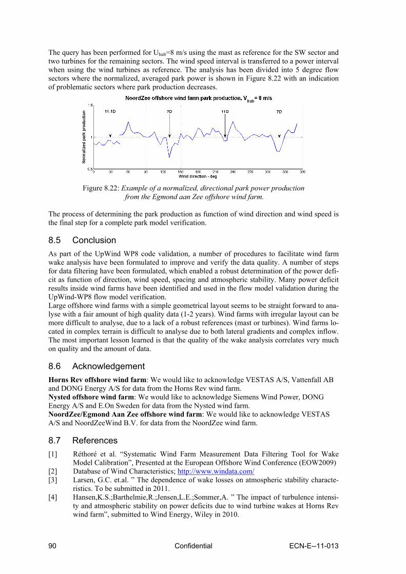
90 Confidential ECN-E--11-013
The query has been performed for Uhub=8 m/s using the mast as reference for the SW sector and two turbines for the remaining sectors. The wind speed interval is transferred to a power interval when using the wind turbines as reference. The analysis has been divided into 5 degree flow sectors where the normalized, averaged park power is shown in Figure 8.22 with an indication of problematic sectors where park production decreases.
Figure 8.22: Example of a normalized, directional park power production
from the Egmond aan Zee offshore wind farm. The process of determining the park production as function of wind direction and wind speed is the final step for a complete park model verification.
8.5 Conclusion As part of the UpWind WP8 code validation, a number of procedures to facilitate wind farm wake analysis have been formulated to improve and verify the data quality. A number of steps for data filtering have been formulated, which enabled a robust determination of the power defi-cit as function of direction, wind speed, spacing and atmospheric stability. Many power deficit results inside wind farms have been identified and used in the flow model validation during the UpWind-WP8 flow model verification. Large offshore wind farms with a simple geometrical layout seems to be straight forward to ana-lyse with a fair amount of high quality data (1-2 years). Wind farms with irregular layout can be more difficult to analyse, due to a lack of a robust references (mast or turbines). Wind farms lo-cated in complex terrain is difficult to analyse due to both lateral gradients and complex inflow. The most important lesson learned is that the quality of the wake analysis correlates very much on quality and the amount of data.
8.6 Acknowledgement Horns Rev offshore wind farm: We would like to acknowledge VESTAS A/S, Vattenfall AB and DONG Energy A/S for data from the Horns Rev wind farm. Nysted offshore wind farm: We would like to acknowledge Siemens Wind Power, DONG Energy A/S and E.On Sweden for data from the Nysted wind farm. NoordZee/Egmond Aan Zee offshore wind farm: We would like to acknowledge VESTAS A/S and NoordZeeWind B.V. for data from the NoordZee wind farm.
8.7 References [1] Réthoré et al. “Systematic Wind Farm Measurement Data Filtering Tool for Wake
Model Calibration”, Presented at the European Offshore Wind Conference (EOW2009) [2] Database of Wind Characteristics; http://www.windata.com/ [3] Larsen, G.C. et.al. ” The dependence of wake losses on atmospheric stability characte-
ristics. To be submitted in 2011. [4] Hansen,K.S.;Barthelmie,R.;Jensen,L.E.;Sommer,A. ” The impact of turbulence intensi-
ty and atmospheric stability on power deficits due to wind turbine wakes at Horns Rev wind farm”, submitted to Wind Energy, Wiley in 2010.

ECN-E--11-013 Confidential 91
9. Recommendation to IEC61400-12-2 Wake sector analysis
May 18th 2006. To the members of the IEC 61400-12-2 expert working group From P.J. Eecen
9.1 Introduction and background Data from the ECN 2.5MW research turbines have been analysed in order to characterise the effect of wakes on nacelle anemometer power performance verification. The ECN Wind turbine Test site Wieringermeer (EWTW) is located in the Netherlands, 35 km East of ECN, Petten. The test site consists of:
• 4 locations with a 100m and a 108m high meteorological mast for testing of prototype wind turbines up to 6MW,
• a wind farm of five research 2.5MW wind turbines equipped for experimental research with another 108m high meteorological mast (MM3),
• and a measurement pavilion with offices and computer center for the measurements. Several ECN research projects are carried out at the EWTW. The collected data comprise:
• Meteorological data measured in the 108m masts • SCADA data (134 signals, ten-minute statistics) from each of the five research turbines,
obtained from Nordex by e-mail on a daily basis • Measured SCADA data (8 signals, 25Hz) from each of the five research turbines • Measured condition monitoring data from five research turbines • Measured loads from one research turbine • Maintenance reports of the research turbines
Data from the research turbines and the meteorological mast MM3 at EWTW are collected and are stored in the Wind Data Management System (WDMS) since September 2004. The Wind Data Management System is a database developed by ECN for storage of data at the signal de-pendent sample rates together with 10-minute statistic values (average, minimum, maximum and standard deviation). For the analysis shown here, 1-minute statistic values have been created. The test site and its surroundings are characterised by flat terrain, consisting of mainly agricultural area, with single farmhouses and rows of trees. The lake IJsselmeer is located at a distance of 2 km east of meteorological masts 1 and 3.
ECN Petten
EWTW

92 Confidential ECN-E--11-013
Research Turbines
Prototype Turbines
Pavilion
Meteo Masts
Research Turbines
Prototype Turbines
Pavilion
Meteo Masts
Figure 9.1 The research turbines are installed in a line which has an angle with respect to
North of 95 degree. The distance between successive turbines is 305m. In the present analysis, turbine 6 is investigated, which is in the wake of the undisturbed turbine 5. The research turbines have hub height of 80m, rotor diameter of 80m and nominal power of 2500 kW.
One-minute averaged data are made and selections are made for the wind direction between 200 and 320 degrees (from the West) and for 'normal' operational modes of the turbine. At these wind directions, turbine 5 is operating in undisturbed wind conditions, while turbine 6 is operat-ing in the wake of turbine 5. For sectors of 2 degrees wide data are selected and with this data nacelle power performance is calculated. The power curves are quite similar and the largest dif-ferences are found in the power coefficient. The largest differences in the power coefficient in-side and outside the wake are found at nacelle wind speeds of 6 to 8m/s. The wind direction reference is chosen to be the nacelle direction of turbine 6, which is in the wake of turbine 5. The nacelle direction of turbine 6 would also be used when nacelle power performance verification would have been applied. To show the effect of the wake of turbine 5 on the produced power by turbine 6 the power deficit is indicated in Figure 9.2: the ratios of the power produced by turbine 5 (free) and turbine 6 (in the wake) are plotted in wind direction bins of 2 degree where turbine 5 produced between 1000 and 2000 kW. From the power deficit, it is clear that the wake is centred around 270 degrees. (from geometry the wake should be at 275 degrees). The (normalized) average power coefficient between 6 and 8m/s based on nacelle power per-formance is also indicated as function of nacelle direction. This is done both for turbine 5 as turbine 6, where turbine 5 indicates the accuracy of the applied method, since there should be minimal effect of wind direction. The normalized power coefficient correlates with the wake of turbine 5. This analysis clearly shows that the power performance analysis is influenced by nearby turbines in a wind direction sector ±15 degrees with respect to the direction of the dis-turbing turbine. Note 1: discussions at the Glasgow meeting expected a hat-like behaviour of the nacelle power performance analysis inside a wake. This behaviour cannot be found in the data analysed of the research turbines.
T-5 T-6

ECN-E--11-013 Confidential 93
Note 2: similar results are obtained using 10-minute averages. Note 3: according IEC 61400-12 the following numbers apply for the sector to be excluded due to wakes of neighbouring and operating wind turbines: (Ln = 305m, Dn = 80m, Ln / Dn = 3.8) and disturbed sector is 60 degrees. The disturbed sector described in IEC 61400-12 is roughly two times larger than we can derive from our analyses.
Figure 9.2. In the upper figure the power deficit of turbine 6 due to the wake of turbine 5 is
indicated (green) together with the (normalized) power coefficient for turbine 5 averaged over 6 to 8m/s (blue). The power deficit is depicted to indicate the angles at which power is influenced by the wake. For turbine 5 the (normalized) power coefficient should be independent of wind direction. In the lower figure the power deficit of turbine 6 due to the wake of turbine 5 is indicated (green) together with the (normalized) power coefficient for turbine 6 averaged over 6 to 8m/s (blue). The (normalized) power coefficient is clearly different within the wake.

94 Confidential ECN-E--11-013
9.1.1 Additional analysis turbulence dependency For the analysis above it would be interesting to know whether the effect of increased cp is dominated by added turbulence due to the wake or due to the nacelle anemometer method. Therefore, the same data of the above analysis (10-minute averaged) have been used to deter-mine the dependency on turbulence. We disregarded the data within the wake. We calculated a normalized cp averaged over 6 to 8m/s and plotted the results. The (normalized) power coeffi-cient increases with increasing turbulence. However, the effect of the wake on the nacelle power performance analysis is significantly larger.
Figure 9.3. This figure illustrates the (normalized) power coefficient for turbine 5 averaged over
6 to 8m/s. The (normalized) power coefficient increases slightly with increasing turbulence.

ECN-E--11-013 Confidential 95
10. Classification of atmospheric stability for offshore wind farms
Kurt S. Hansen, Department of Mechanical Engineering, DTU Validation of power deficit and structural wind turbine fatigue loads on turbines in wind farms requires knowledge of the stability conditions. As part of the wake analysis performed on the Horns Rev offshore wind farm, a robust classification of the atmospheric stability has been es-tablished, based on the Bulk Richardson number.
10.1 Introduction Determination of power deficit and structural wind turbine fatigue loads on turbines operating in wind farms requires knowledge of the stability conditions. As part of the wake analysis at Horns Rev offshore wind farm, it has been necessary to develop, implement and verify a classification method for the atmospheric stability. The Horns Rev Wind farm consists of 80 wind turbines, arranged in a regular shape together with three offshore masts as shown in Figure 10.1. The wind farm includes one mast NW to the wind farm and two masts E east to the wind farm. The wind farm operation has been recorded during 4 years (2005 – 2008) and the wake analysis has been performed on a merger of wind turbine SCADA data and meteorological data.
10.1.1 Instrumentation The Horns Rev wind farm includes three masts M2, M6 and M7. M2 was erected prior to the wind farm installation and has been used to determine the offshore wind resources and wind conditions, which was [partly] used to establish the wind farm design specification. Mast M2 is located approximately 2 km NW of the wind farm and is measuring free, undisturbed wind speeds more than 75% of the time. The instrumentation includes cups, vanes, thermometers and a sonic anemometer, as sketched in Figure 10.2. All measurements from these masts have been stored as 10-minute statistics in terms of mean, standard deviation, minimum and maximum values. M2 has been operational in the period 1999-2006 [1], but unfortunately there has only been one year overlap between mast and wind farm operation. Furthermore the instrumentation was not maintained well during 2005, which resulted in a lack of quality data. M6 & M7 were installed in 2003, as part of the offshore wake measurement program and are located 2 and 6 km east of the wind farm as indicated in Figure 10.1. The mast instrumentation is identical and is located between 20 to 70 m above mean sea level - as indicated in Figure 10.2. The mast setup and the measurements representing the first period of operation have been reported in [2]. The purpose was to measure the wake properties and the masts are located in-side the wind farm wake more than 60% of time. M2 was equipped with a sonic anemometer, 50 m above sea level and a huge amount of time series has been stored in a wind repository [3]. Unfortunately the sonic anemometer was mounted on a boom pointing towards SW; which reduced the free, undisturbed inflow sector considerably 225±45°.

96 Confidential ECN-E--11-013
Figure 10.1: Layout of Horns rev wind farm, including 3 offshore masts.
Figure 10.2: Horns Rev offshore wind farm mast instrumentation.

ECN-E--11-013 Confidential 97
10.2 Determination of atmospheric stability. The atmospheric stability can be expressed with the stability parameter z’/L where L is the Mo-nin-Obukov length L and z’ is a reference height. Previously the stability parameter has been determined as part of several research project mainly focusing on onshore locations with suc-cess. The wake analysis in UpWind WP8 required a stability classification and during this project three different methods have been evaluated with respect to the available signals from the Horns Rev site. Different solutions have been presented during the recent years to establish a classification and the most promising is based on the temperature gradient [4, 5]. A short de-scription is given below, including a short summery of the main findings and problems. The problems were caused by the limited data coverage, poor data quality and the wake conditions.
10.2.1 Gradient method. The atmospheric stability parameter z’/L has been calculated according to the gradient method applied on year 2005 measurements and was based on either the difference between 1) water and air or 2) air and air temperatures, from the wake mast M7; which had a very good signal quality and a high availability. The Richardson number (Ri) is calculated with (eq. 1):
( ) ( )( ) ( )( )70 209.81 / 273.15 / / /u u l T VRi t t t h sqr U U h= + × − Δ − Δ ( 10.1 ) The signals from M7, used in the stability calculation are listed in Table 10.1, but situations with reduced wind speed at hub height caused by the wind farm wake were not been eliminated.
Table 10.1: Sensors used to determine the atmospheric stability parameter. Sensor Air/water Air/air tu - degC h = 64 m (asl) h = 64 m tl - degC h = -3 m (bsl) h = 64 m U70 h = 70 m h = 70 mU20 h = 20 m h = 20 mz’ 31 m 37.5 m
The stability parameter z’/L has been derived from the Ri number according to (10.2), (10.3) and (10.4):
z’/L=Ri; for Ri≤0; ( 10.2 ) z’/L=Ri/(1-5Ri); for 0<Ri<0.2 ( 10.3 ) z’/L=2×z’×Ri; for Ri≥0.2; ( 10.4 ) The relation between speed ratio and the stability parameter are plotted in Figure 10.3 and de-monstrates a clear correlation for negative stability parameters, while positive stability results in a large scatter.
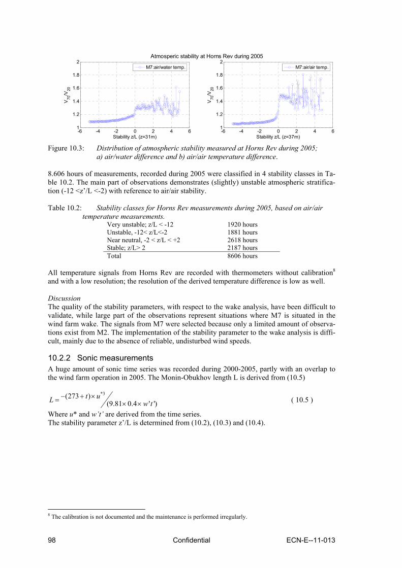
98 Confidential ECN-E--11-013
-6 -4 -2 0 2 4 61
1.2
1.4
1.6
1.8
2
Stability z/L (z=31m)
V70
/V20
-6 -4 -2 0 2 4 61
1.2
1.4
1.6
1.8
2
Stability z/L (z=37m)
V70
/V20
M7:air/air temp.M7:air/water temp.
Atmosperic stability at Horns Rev during 2005
Figure 10.3: Distribution of atmospheric stability measured at Horns Rev during 2005;
a) air/water difference and b) air/air temperature difference. 8.606 hours of measurements, recorded during 2005 were classified in 4 stability classes in Ta-ble 10.2. The main part of observations demonstrates (slightly) unstable atmospheric stratifica-tion (-12 <z’/L <-2) with reference to air/air stability. Table 10.2: Stability classes for Horns Rev measurements during 2005, based on air/air
temperature measurements. Very unstable; z/L < -12 1920 hours Unstable, -12< z/L<-2 1881 hours Near neutral, -2 < z/L < +2 2618 hours Stable; z/L> 2 2187 hours Total 8606 hours
All temperature signals from Horns Rev are recorded with thermometers without calibration8 and with a low resolution; the resolution of the derived temperature difference is low as well. Discussion The quality of the stability parameters, with respect to the wake analysis, have been difficult to validate, while large part of the observations represent situations where M7 is situated in the wind farm wake. The signals from M7 were selected because only a limited amount of observa-tions exist from M2. The implementation of the stability parameter to the wake analysis is diffi-cult, mainly due to the absence of reliable, undisturbed wind speeds.
10.2.2 Sonic measurements A huge amount of sonic time series was recorded during 2000-2005, partly with an overlap to the wind farm operation in 2005. The Monin-Obukhov length L is derived from (10.5)
*3(273 )(9.81 0.4 ' ')
t uL w t− + ×= × × ( 10.5 )
Where u* and w’t’ are derived from the time series. The stability parameter z’/L is determined from (10.2), (10.3) and (10.4).
8 The calibration is not documented and the maintenance is performed irregularly.

ECN-E--11-013 Confidential 99
Atmosperic stability distribution at Horn Rev, h=50based on 11000 hours sonic measurements.
0%
5%
10%
15%
20%
25%
30%
-3 -2 -1 0 1 2 3cL
NESW
Figure 10.4: Stability classification based on sonic measurements. The huge amount of stability parameters have been classified according to the classification scheme in Table 10.3 and the classification distribution for the 4 main directions (N, E, S & W) are shown in Figure 10.4. Discussion The quality of the calculated stability parameters seems to be fine and the distribution seems to be applicable. Unfortunately a very limited overlap between sonic measurements and the wind farm operation exist and this is not sufficient for a proper validation of this method. It needs to be verified whether the sonic height of 50 m is applicable for offshore locations or a lower off-shore measuring height should be recommended.
10.2.3 Bulk-Richardson number The flow conditions, expressed in terms of atmospheric stability classes, have been established with reference to a Bulk-Richardson approach evaluated in [4, 5, 6]. The Rib number is derived from a single wind speed observation (Uh), measured at 15 - 20 m height above mean sea level combined9 with the air and water temperature difference (Δt) from (10. 6). The Obukhov length, L is derived from the Rib number (10.7) and (10.8) as described in [6] including the classifica-tion of the atmospheric stability.
29.81 ( / 0.01) / ( ( / ) )b hRi t h T U h= − × Δ Δ − × ( 10.6 )
'/ 10 bz L Ri= × for unstable stratification ( 10.7 )
10'/1 5
b
b
Riz LRi
×=
− × for stable stratification ( 10.8 )
The stability parameter has been derived for all available measurement (M2, M6 and M7); which were recorded before, during and after the wind farm installation. The wind speed signal at the lowest available height has been selected10 to minimize the wake reducing effect from the wind farm. 9 A zero wind speed at sea level is assumed. 10 The lowest blade-tip position is 10-14 m above the measuring height but still the wake expansion could influence the recorded wind signal.

100 Confidential ECN-E--11-013
The stability classification has been adapted from a previous onshore classification [7] with ref-erence to the Obukhov length L and is listed in Table 10.3. Table 10.3: Classification of atmospheric stability at Horns Rev, based on Obukhov length L.
Class Obukhov length [m] Atmosperic stability classcL=-3 -100 ≤ L ≤ -50 Very unstable (vu)cL=-2 -200 ≤ L ≤ -100 Unstable (u)cL=-1 -500 ≤ L ≤ -200 Near unstable (nu)cL=0 |L|>500 Neutral (n)cL=1 200 ≤ L ≤ 500 Near stable (ns)cL=2 50 ≤ L ≤ 200 Stable (s)cL=3 10 ≤ L ≤ 50 Very stable (vs)
The use of the air-water temperature difference to define stability classes tends to limit the number of observations in the near-neutral class. A further issue at Horns Rev is that tempera-tures are measured to a precision of 0.1 ºC. At moderate temperatures and at moderate/high wind speeds this inaccuracy will lead to minor differences (e.g. observations being placed in the very stable class rather than the stable class). However when temperature differences are small, the measurement precision could lead to erroneous classification. Hence the neutral and near-neutral classes (cL=-1, 0, 1) should be seen as a broad grouping. The classification has been va-lidated for four flow directions and Table 10.4 lists the amount of available hours. The valida-tion is performed for a wind speed interval of 5.5 – 10.5 m/s at hub height (70m); which was used in the wake analysis, performed in UpWind WP8. Table 10.4: Number of hours representing wind speeds interval of 6 - 10 m/s, representing a
60° inflow sectors. 5.5 - 10.5 m/s M2 M6 M7
hours hours hoursN (partly free) 1829 1773 6821
E (wake) 1701 1604 6811S (partly free) 2458 2149 7881
W (wake) 2548 2254 8053 Validation for northern wind direction The free M2 wind speed measurements, recorded 15m above mean sea level, have been used to classify the stability. A northern flow direction 0±30° has been validated according to the rec-orded number of hours in Table 10.4, with an operating wind farms.
HR-M6; sector: <=30 & >330 deg; 5.5 < V70 <= 10.5 m/s
0%
5%
10%
15%
20%
25%
30%
35%
40%
-3 -2 -1 0 1 2 3
cL
M2M6M7
Figure 10.5: Comparison of classification results, based on measurements from M2, M6 & M7
at Horns Rev recorded in the northern sector.
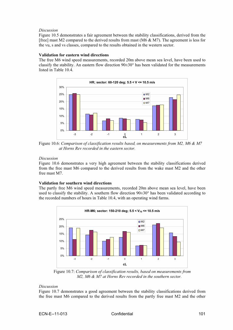
ECN-E--11-013 Confidential 101
Discussion Figure 10.5 demonstrates a fair agreement between the stability classifications, derived from the [free] mast M2 compared to the derived results from mast (M6 & M7). The agreement is less for the vu, s and vs classes, compared to the results obtained in the western sector. Validation for eastern wind directions The free M6 wind speed measurements, recorded 20m above mean sea level, have been used to classify the stability. An eastern flow direction 90±30° has been validated for the measurements listed in Table 10.4.
HR; sector: 60-120 deg; 5.5 < V <= 10.5 m/s
0%
5%
10%
15%
20%
25%
30%
-3 -2 -1 0 1 2 3cL
M2M6M7
Figure 10.6: Comparison of classification results based, on measurements from M2, M6 & M7
at Horns Rev recorded in the eastern sector. Discussion Figure 10.6 demonstrates a very high agreement between the stability classifications derived from the free mast M6 compared to the derived results from the wake mast M2 and the other free mast M7. Validation for southern wind directions The partly free M6 wind speed measurements, recorded 20m above mean sea level, have been used to classify the stability. A southern flow direction 90±30° has been validated according to the recorded numbers of hours in Table 10.4, with an operating wind farms.
HR-M6; sector: 150-210 deg; 5.5 < V70 <= 10.5 m/s
0%
5%
10%
15%
20%
25%
-3 -2 -1 0 1 2 3
cL
M2M6M7
Figure 10.7: Comparison of classification results, based on measurements from
M2, M6 & M7 at Horns Rev recorded in the southern sector.
Discussion Figure 10.7 demonstrates a good agreement between the stability classifications derived from the free mast M6 compared to the derived results from the partly free mast M2 and the other

102 Confidential ECN-E--11-013
free mast M7 for a southern flow sector. The agreement is less for the vu and vs classes, com-pared to the other sectors. Validation for western wind directions The free M2 wind speed measurements, recorded 15m above mean sea level, have been used to classify the stability. A westerly flow direction of 270±30° has been validated according to the recorded numbers of hours in Table 10.4, with an operating wind farms.
HR; sector: 240-300 deg; 5.5 < V <= 10.5 m/s
0%
5%
10%
15%
20%
25%
30%
35%
40%
-3 -2 -1 0 1 2 3
cL
M2M6M7
Figure 10.8: Comparison of classification results, based on measurements from
M2, M6 & M7 at Horns Rev recorded in the western sector. Discussion Figure 10.8 demonstrates an very good agreement between the stability classifications derived from the free mast M2 compared the derived results from the wake masts (M6 & M7) for a western flow sector. This is the most important flow sector for the wake analysis and the devia-tions related the stable and very stable classes complement each other. Conclusion: The validation reveals a high level of confidence between the different atmospheric stability classifications when using measurements recorded at low heights. The main difference is proba-bly related to the quality of the measurements and seems to be isolated within the stable or the unstable classes. This enables us to use the most appropriate measurements, when categorizing the flow deficits near wind farms. A sector-wise validation of the stability classification shows no large discrepancy between “wake” and “no-wake” situation.
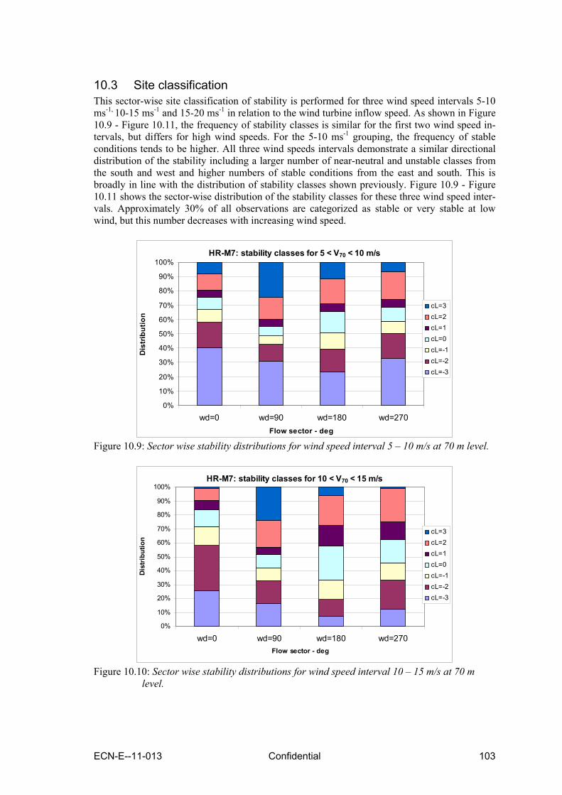
ECN-E--11-013 Confidential 103
10.3 Site classification This sector-wise site classification of stability is performed for three wind speed intervals 5-10 ms-1, 10-15 ms-1 and 15-20 ms-1 in relation to the wind turbine inflow speed. As shown in Figure 10.9 - Figure 10.11, the frequency of stability classes is similar for the first two wind speed in-tervals, but differs for high wind speeds. For the 5-10 ms-1 grouping, the frequency of stable conditions tends to be higher. All three wind speeds intervals demonstrate a similar directional distribution of the stability including a larger number of near-neutral and unstable classes from the south and west and higher numbers of stable conditions from the east and south. This is broadly in line with the distribution of stability classes shown previously. Figure 10.9 - Figure 10.11 shows the sector-wise distribution of the stability classes for these three wind speed inter-vals. Approximately 30% of all observations are categorized as stable or very stable at low wind, but this number decreases with increasing wind speed.
HR-M7: stability classes for 5 < V70 < 10 m/s
0%
10%
20%
30%
40%
50%
60%
70%
80%
90%
100%
wd=0 wd=90 wd=180 wd=270Flow sector - deg
Dis
trib
utio
n
cL=3cL=2cL=1cL=0cL=-1cL=-2cL=-3
Figure 10.9: Sector wise stability distributions for wind speed interval 5 – 10 m/s at 70 m level.
HR-M7: stability classes for 10 < V70 < 15 m/s
0%
10%
20%
30%
40%
50%
60%
70%
80%
90%
100%
wd=0 wd=90 wd=180 wd=270Flow sector - deg
Dist
ribut
ion
cL=3cL=2cL=1cL=0cL=-1cL=-2cL=-3
Figure 10.10: Sector wise stability distributions for wind speed interval 10 – 15 m/s at 70 m
level.
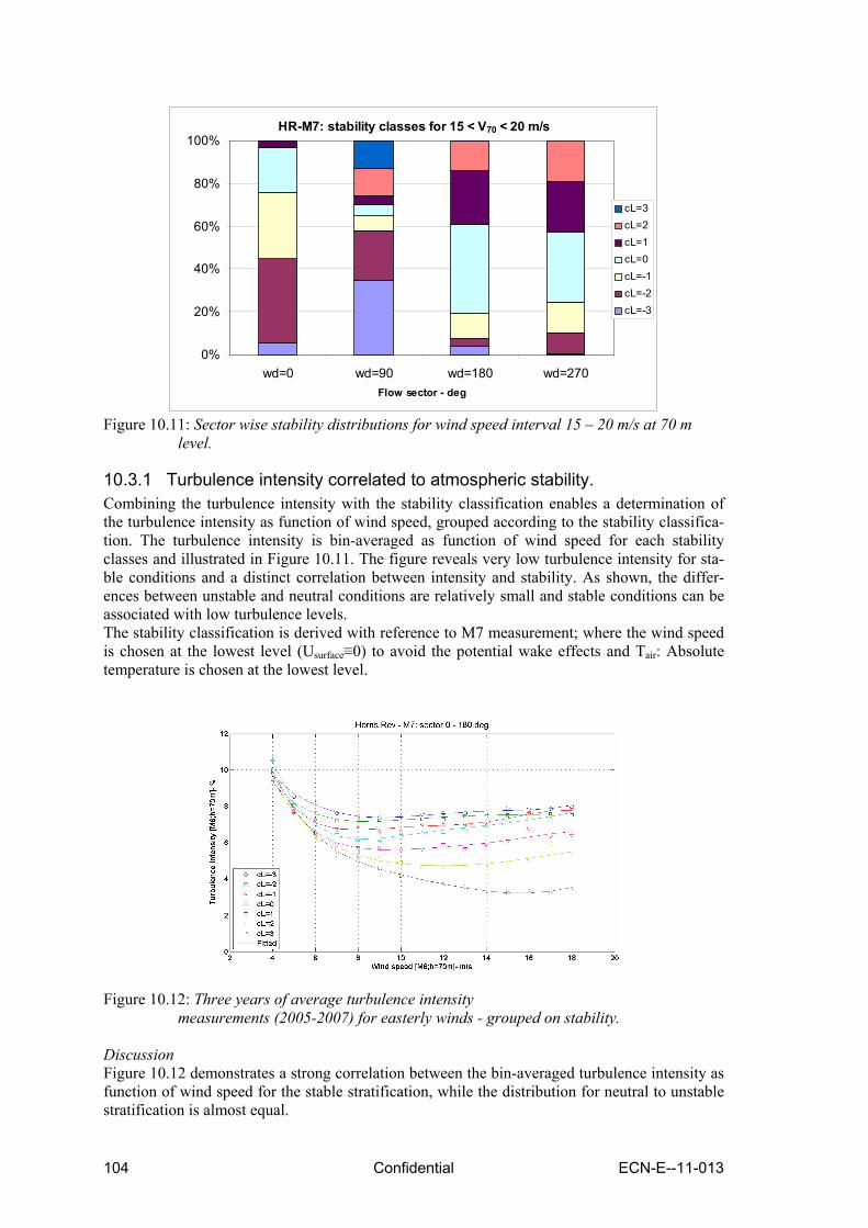
104 Confidential ECN-E--11-013
HR-M7: stability classes for 15 < V70 < 20 m/s
0%
20%
40%
60%
80%
100%
wd=0 wd=90 wd=180 wd=270Flow sector - deg
cL=3cL=2cL=1cL=0cL=-1cL=-2cL=-3
Figure 10.11: Sector wise stability distributions for wind speed interval 15 – 20 m/s at 70 m
level.
10.3.1 Turbulence intensity correlated to atmospheric stability. Combining the turbulence intensity with the stability classification enables a determination of the turbulence intensity as function of wind speed, grouped according to the stability classifica-tion. The turbulence intensity is bin-averaged as function of wind speed for each stability classes and illustrated in Figure 10.11. The figure reveals very low turbulence intensity for sta-ble conditions and a distinct correlation between intensity and stability. As shown, the differ-ences between unstable and neutral conditions are relatively small and stable conditions can be associated with low turbulence levels. The stability classification is derived with reference to M7 measurement; where the wind speed is chosen at the lowest level (Usurface≡0) to avoid the potential wake effects and Tair: Absolute temperature is chosen at the lowest level.
Figure 10.12: Three years of average turbulence intensity
measurements (2005-2007) for easterly winds - grouped on stability.
Discussion Figure 10.12 demonstrates a strong correlation between the bin-averaged turbulence intensity as function of wind speed for the stable stratification, while the distribution for neutral to unstable stratification is almost equal.
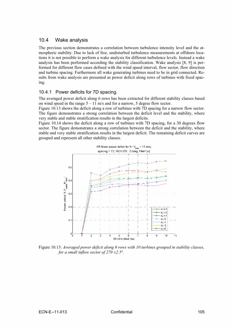
ECN-E--11-013 Confidential 105
10.4 Wake analysis The previous section demonstrates a correlation between turbulence intensity level and the at-mospheric stability. Due to lack of free, undisturbed turbulence measurements at offshore loca-tions it is not possible to perform a wake analysis for different turbulence levels. Instead a wake analysis has been performed according the stability classification. Wake analysis [8, 9] is per-formed for different flow cases defined with the wind speed interval, flow sector, flow direction and turbine spacing. Furthermore all wake generating turbines need to be in grid connected. Re-sults from wake analysis are presented as power deficit along rows of turbines with fixed spac-ing.
10.4.1 Power deficits for 7D spacing. The averaged power deficit along 6 rows has been extracted for different stability classes based on wind speed in the range 5 – 11 m/s and for a narrow, 5 degree flow sector. Figure 10.13 shows the deficit along a row of turbines with 7D spacing for a narrow flow sector. The figure demonstrates a strong correlation between the deficit level and the stability, where very stable and stable stratification results in the largest deficits. Figure 10.14 shows the deficit along a row of turbines with 7D spacing, for a 30 degrees flow sector. The figure demonstrates a strong correlation between the deficit and the stability, where stable and very stable stratification results in the largest deficit. The remaining deficit curves are grouped and represent all other stability classes.
Figure 10.13: Averaged power deficit along 6 rows with 10 turbines grouped in stability classes,
for a small inflow sector of 270 ±2.5°.
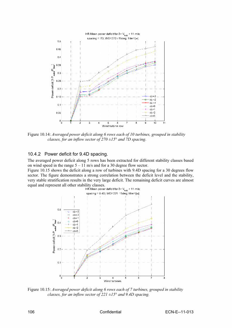
106 Confidential ECN-E--11-013
Figure 10.14: Averaged power deficit along 6 rows each of 10 turbines, grouped in stability
classes, for an inflow sector of 270 ±15° and 7D spacing.
10.4.2 Power deficit for 9.4D spacing. The averaged power deficit along 5 rows has been extracted for different stability classes based on wind speed in the range 5 – 11 m/s and for a 30 degree flow sector. Figure 10.15 shows the deficit along a row of turbines with 9.4D spacing for a 30 degrees flow sector. The figure demonstrates a strong correlation between the deficit level and the stability, very stable stratification results in the very large deficit. The remaining deficit curves are almost equal and represent all other stability classes.
Figure 10.15: Averaged power deficit along 6 rows each of 7 turbines, grouped in stability
classes, for an inflow sector of 221 ±15° and 9.4D spacing.
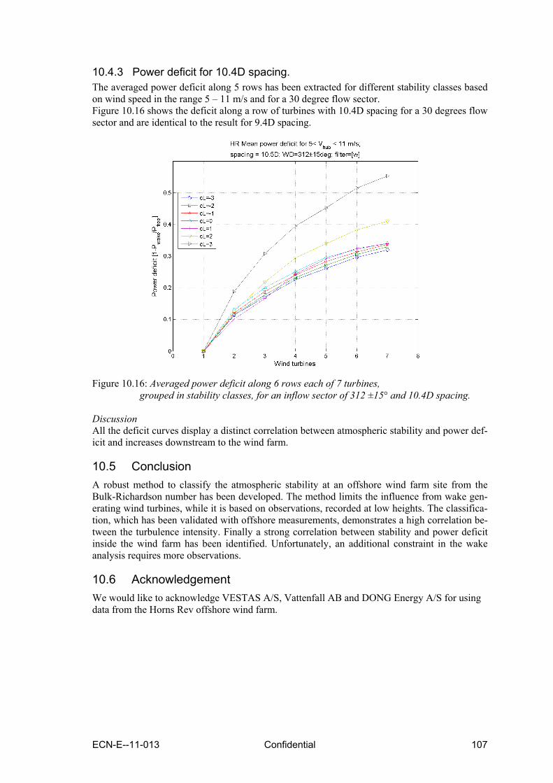
ECN-E--11-013 Confidential 107
10.4.3 Power deficit for 10.4D spacing. The averaged power deficit along 5 rows has been extracted for different stability classes based on wind speed in the range 5 – 11 m/s and for a 30 degree flow sector. Figure 10.16 shows the deficit along a row of turbines with 10.4D spacing for a 30 degrees flow sector and are identical to the result for 9.4D spacing.
Figure 10.16: Averaged power deficit along 6 rows each of 7 turbines,
grouped in stability classes, for an inflow sector of 312 ±15° and 10.4D spacing. Discussion All the deficit curves display a distinct correlation between atmospheric stability and power def-icit and increases downstream to the wind farm.
10.5 Conclusion A robust method to classify the atmospheric stability at an offshore wind farm site from the Bulk-Richardson number has been developed. The method limits the influence from wake gen-erating wind turbines, while it is based on observations, recorded at low heights. The classifica-tion, which has been validated with offshore measurements, demonstrates a high correlation be-tween the turbulence intensity. Finally a strong correlation between stability and power deficit inside the wind farm has been identified. Unfortunately, an additional constraint in the wake analysis requires more observations.
10.6 Acknowledgement We would like to acknowledge VESTAS A/S, Vattenfall AB and DONG Energy A/S for using data from the Horns Rev offshore wind farm.

108 Confidential ECN-E--11-013
10.7 References [1] Sommer,A.;Hansen,K.S. “Wind Resources at Horns Rev. 2002”, Techwise:Eltra PSO-
2000 Proj. nr. EG-05 3248. DK-7000 Fredericia. [2] Sørensen,P.B.;Hansen K.S. “Wake effect east of the Horns Rev offshore wind farm.”
2002, Elkraft System:PSO-F&U 2002/FU 2103. DK-7000 Fredericia. [3] Database of Wind Characteristics; http://www.windata.com/ [4] Lange, B. et.al. "Modelling the vertical wind speed and turbulence intensity profiles at
prospective offshore wind farm sites" In: Proceedings CD-ROM. 2002 global wind-power conference and exhibition, Paris (FR), 2-5 Apr 2002
[5] Jens Tambke et.al. "Offshore Meteorology for Multi-Mega-Watt Turbines" presented at EWEC 2006
[6] Larsen, G.C. et.al. ” The dependence of wake losses on atmospheric stability characte-ristics. To be submitted in 2011.
[7] Penã, A.,et.al. "Extending the wind profile much higher than the surface layer", pre-sented at EWEC2009 in Marseille, FR 16-19 March 2009.
[8] Hansen,K.S.;Barthelmie,R.;Jensen,L.E.;Sommer,A. ” The impact of turbulence intensi-ty and atmospheric stability on power deficits due to wind turbine wakes at Horns Rev wind farm”, submitted to Wind Energy, Wiley in 2010.
[9] Barthelmie,R. et.al. "Flow and wakes in large wind farms:Final report; Appendix 6: Guideline to wind farm wake analysis"; Report number Risø-R-1765(EN), January 2011
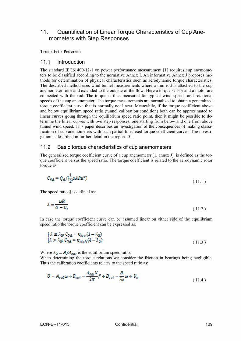
ECN-E--11-013 Confidential 109
11. Quantification of Linear Torque Characteristics of Cup Ane-mometers with Step Responses
Troels Friis Pedersen
11.1 Introduction The standard IEC61400-12-1 on power performance measurement [1] requires cup anemome-ters to be classified according to the normative Annex I. An informative Annex J proposes me-thods for determination of physical characteristics such as aerodynamic torque characteristics. The described method uses wind tunnel measurements where a thin rod is attached to the cup anemometer rotor and extended to the outside of the flow. Here a torque sensor and a motor are connected with the rod. The torque is then measured for typical wind speeds and rotational speeds of the cup anemometer. The torque measurements are normalized to obtain a generalized torque coefficient curve that is normally not linear. Meanwhile, if the torque coefficient above and below equilibrium speed ratio (tunnel calibration condition) both can be approximated to linear curves going through the equilibrium speed ratio point, then it might be possible to de-termine the linear curves with two step responses, one starting from below and one from above tunnel wind speed. This paper describes an investigation of the consequences of making classi-fication of cup anemometers with such partial linearised torque coefficient curves. The investi-gation is described in further detail in the report [5].
11.2 Basic torque characteristics of cup anemometers The generalised torque coefficient curve of a cup anemometer [1, annex J] is defined as the tor-que coefficient versus the speed ratio. The torque coefficient is related to the aerodynamic rotor torque as:
( 11.1 )
The speed ratio is defined as:
( 11.2 )
In case the torque coefficient curve can be assumed linear on either side of the equilibrium speed ratio the torque coefficient can be expressed as:
( 11.3 )
Where is the equilibrium speed ratio. When determining the torque relations we consider the friction in bearings being negligible. Thus the calibration coefficients relates to the speed ratio as:
( 11.4 )

110 Confidential ECN-E--11-013
11.3 Linearized torque characteristics of a typical cup anemometer The analysis is based on measurements of torque coefficients made in the FOI wind tunnel by Jan-Åke Dahlberg in the ACCUWIND project [2]. The cup anemometers that were considered are shown in Table 11.1 with some details.
Table 11.1 Main data of cup anemometers analysed in ACCUWIND project [2] NRG RISØ THIES-FC VAISALA VECTOR Cup diameter (mm) 51 70 80 54 51 Projected cup area A (mm2) 2000 3850 5030 2290 2040 Rotor diameter (mm) 191 186 240 184 155 Radius to cup centre R (mm)
70 58 80 65 52
Pulses/rev 2 2 37 14 25 Rotor inertia I (kg m2) 1.01·10-4 0.992·10-4 2.8888·10-4 0.6141·10-4 0.441·10-4 The torque coefficient curves from [2] were linearized on either side of the equilibrium speed ratio, forced through the point of equilibrium speed ratio. The linearized torque coefficient data are shown in Table 11.2 together with derived time constants from inertia in table 1 and with a standard air density of 1.23kg/m3.
Table 11.2 Linearized torque coefficient data from linearization of Main data of cup anemometers analysed in ACCUWIND project [2]
NRG RISØ THIES-FC VAISALA VECTOR Equilibrium speed ratio 0.28461 0.29653 0.28022 0.28964 0.26177 Slope at low speed ratios -6.5282 -4.9590 -4.6520 -4.8867 -6.6914 Slope at high speed ratios
-6.3595 -6.2140 -5.6901 -4.7652 -6.3128
Ratio 1.0265 0.7980 0.8176 1.0255 1.0600
11.4 Classification of cup anemometers with linear torque The torque coefficient curves from the ACCUWIND project [2] were applied for classification according to the standard IEC61400-12-1 [1]. The results with the full torque coefficient curves and tilt response data measured in the FOI wind tunnel were compared with the results using the linear torque coefficient data from Table 11.2. The results are shown in Table 11.3.
Table 11.3 Classification of Risø P2546a using Cm curves or two linearized curves Class A Class A
linearized Class B Class B
linearized Risø P2546 1.39628 1.39404 (-0.16%) 5.09301 5.0887 (-
0.09%) Thies First Class 1.78074 1.76010 (-1.17%) 3.87461 3.89775
(+0.59%) Vector 1.82939 1.84430
(+0.81%) 4.48396 4.26761 (-
5.07%) Vaisala 2.22558 2.14491 (-3.63%) 11.9380 11.8207 (-
0.98%) NRG Max40 2.41664 2.52689
(+4.36%) 8.28358 7.98579 (-
3.73%)

ECN-E--11-013 Confidential 111
The comparison of classification results from Table 11.3 shows very good results. The largest deviation is 5.07% on the classification value. Considering that other uncertainties are signifi-cant in the whole classification process, this is an indication that linearized torque coefficient curves can be considered sufficient for classification.
11.5 Step response measurement procedures There are two standards that consider step response measurements. The recommended practice document IEA-11 [3] considers step response measurements in or-der to determine the time constant and the distant constant. The step response model used in the IEA-11 document is described as:
( 11.5 )
In IEA-11 a linear fitting of a conversion of the step response function is proposed:
( 11.6 )
The standard ISO 17713-1 [4] on wind tunnel test methods for rotating anemometer perfor-mance describes step response measurements in order to determine the distance constant. The model used is described as:
( 11.7 )
And the distance constant is determined from:
( 11.8 ) The standard requires 10 step response measurements made at 5m/s and 10m/s. The time con-stant is determined from data measured between 30% and 74% of the tunnel wind speed, and the distance constant is determined by multiplying the tunnel wind speed with the time constant. When we want to determine torque coefficient characteristics from step response measurements we have to find an appropriate method for determination of the slopes of the torque coefficient curves below and above the equilibrium speed ratio. Theoretical considerations documents and derive such a procedure [6]. The result is that the slopes can be derived as:
( 11.9 )

112 Confidential ECN-E--11-013
11.6 Step response measurements – an example
An example of a step-up response made by WindGuard is shown in Figure 11.1. The cup ane-mometer is a Risø P2546 and the tunnel wind speed is 5m/s. Using the IEA-11 fitting procedure we get the logarithmic expression as function of time as shown in Figure 11.2.
-20%
0%
20%
40%
60%
80%
100%
120%
0,0 0,5 1,0 1,5 2,0 2,5 3,0 3,5 4,0
rela
tive
spee
d
Time t (s)
Step-up response Risø anemometer at 5 m/s
Figure 11.1 Step-up response of Risø P2546 cup anemometer at 5m/s tunnel wind speed.
y = -1,4982x + 1,5649
-7
-6
-5
-4
-3
-2
-1
0
0,0 0,5 1,0 1,5 2,0 2,5 3,0 3,5 4,0
ln(e
xpre
ssio
n)
Time t (s)
ln(expression) in IEA-11 step response fitting, 50-98% of data
Figure 2
Figure 11.2 ln-expression from IEA-11 step response fitting procedure using 50-98% of step-up data

ECN-E--11-013 Confidential 113
Figure 11.3 shows a speed-down response of the same Risø cup anemometer, first speeded up to 200%, and Figure 11.4 shows the ln-expression for a relative speed range of 150-102%, which seems to cover quite well the essential part of the step response.
60%
80%
100%
120%
140%
160%
180%
200%
220%
240%
0,0 0,5 1,0 1,5 2,0 2,5 3,0 3,5 4,0 4,5 5,0
rel.
spee
d
time / m/s
Step-down response Risoe anemometer at 5 m/s
Figure 11.3 Step-down response of Risø P2546 cup anemometer at 5m/s tunnel wind speed.
y = -1,5969x + 2,4083
-4,5
-4,0
-3,5
-3,0
-2,5
-2,0
-1,5
-1,0
-0,5
0,0
0,0 0,5 1,0 1,5 2,0 2,5 3,0 3,5 4,0 4,5 5,0
ln(e
xpre
ssio
n)
Time t (s)
ln(expression) in IEA-11 step response fitting, 150-102%
Figure 11.4 ln-expression from IEA-11 step response fitting procedure using 150-102% of step-
down data.
The step responses were performed more than once. Table 11.4 shows the results, where they are compared with the values from linearization of the torque curves from the ACCUWIND project.

114 Confidential ECN-E--11-013
Table 11.4 Slopes of linear torque coefficient curves for Risø P2546 cup anemometer de-termined with torque measurements according to [2] and with step responses Risø torque coefficient slopes
Torque measurements ACCUWIND linearised
Torque measurements step responses
Ratio step/ACCUW
Equlibrium speed ratio 0.29653 Slope at low speed ratios
-4.9590 -3.493 0.704
Slope at high speed ratios
-6.2140 -4.088 0.658
Ratio 0.7980 0.8545 1.071 From Table 11.4 it is seen that the step response method gives about 30% lower torque coeffi-cient slopes than the linearized torque from the measurements in the ACCUWIND project. The torque coefficient slope values are proportional to the rotor inertia and the slopes of the ln-expressions, but reverse proportional to the time constants. The reason for the difference might be due to additional inertia in the rotating test equipment during the tests, but the cause has not been identified. The deviation is slope ratios is only 7%. It can be shown that the maximum overspeeding (at high frequencies) is only dependent on the ratio between the slopes of the tor-que coefficient curves. In this case it might be satisfactory for the classification only to know the ratio with a good accuracy.
11.7 Conclusions The step response model of the IEA-11 document intrinsically leads to linear torque coefficient curves for step responses from low or high speed ratios. The slopes of the linear torque coeffi-cient curves can thus be determined from the step response time constants. The intercept of the linear torque coefficient curves, which is the equilibrium speed ratio, is determined from the normal wind tunnel calibration gain value. The standard ISO 17713-1 recommends step re-sponse data in the speed ratio range 30-75% to be used. This seems to be in a range that is out-side of the usual range being used in classification according to IEC61400-12-1. In practice, a range closer to equilibrium speed ratios should be used; 50-98% for speed-up step responses and 150-102% for speed-down step responses. The step response measurements can satisfactorily determine linear torque coefficient characteristics of cup anemometers with the only assumption that the friction in bearings is negligible with respect to determination of aerodynamic torque characteristics. Meanwhile, slope values were found to be about 30% too low. The step response method may be improved by adding more inertia to the rotor to extend the data and to reduce torque ripples due to the cups, and by determining the rotor inertia with high accuracy.
11.8 References
[1] IEC 61400-12-1, 2005 Wind turbines – Part 12-1: Power performance measurements of electricity producing wind turbines
[2] Pedersen TF, Dahlberg J-Å, Busche P, “ACCUWIND – Classification of Five Cup Ane-mometers According to IEC61400-12-1”, Risø-R-1556(EN), May 2006
[3] IEA-11 Wind Speed Measurement and Use of Cup Anemometry, Recommended Practices for Wind Turbine Testing and Evaluation, 1999
[4] ISO 17713-1, 2007 Meteorology – Wind Measurements – Part 1: Wind tunnel test me-thods for rotating anemometer performance
[5] Pedersen TF, “Quantification of Linear Torque Characteristics of Cup Anemometers with Step Responses”, Risø-I-3131(EN), February 2011

ECN-E--11-013 Confidential 115
12. Generics of nacelle anemometry
Troels F. Pedersen
12.1 Introduction The generic influence of the flow induction on nacelle anemometry was studied lately by Sten Frandsen. He published a paper at the EWEC conference 2009 in Marseille [1] with five co-authors, including the author of this article. The paper was the last work of Sten Frandsen on nacelle anemometry, which was a dedicated topic in his large variety of research. He sadly passed away autumn 2010. This article is an extract from his paper. Nacelle anemometry is the state of the art wind measurement method for turbine regulation and performance verification. The option of using the nacelle anemometer when determining the power curve of a wind turbine is attractive since it is much cheaper than erecting a separate me-teorological mast and simpler since all data signals are already recorded in the wind turbine’s control and data recording system. In particular, the consequences of the effect of rotor flow in-duction must be dealt with, but also the local flow distortion over the nacelle where nacelle anemometry is positioned is necessary to consider in turbine regulation and performance verifi-cation. Thus, if the power changes it must a priori be expected that the rotor flow speed changes, even if the free wind speed is unchanged. In that case the calibration of the nacelle anemometer is changed, effectively introducing an error to the test. In the paper of Sten Frandsen [1], previ-ous investigations of nacelle anemometry is reviewed, the relevance of Betz theory is investi-gated by means of CFD computations, and the generic errors caused by the rotor flow induction is evaluated, estimated and exemplified.
12.2 Review of nacelle anemometry Nacelle anemometry as an option for power performance verification was identified in the be-ginning of the 1990'ies, where some developers and manufacturers started to apply nacelle anemometry in the context of commercial contracts. The method included the calibration of the nacelle anemometer, already installed on the top of the nacelle of the wind turbine, against an unobstructed met mast at a reasonably flat location in the wind farm. The method was first men-tioned in 1994 [2], which deals with trends in power performance measurement techniques and recommendations with respect to positioning of the wind sensor on the nacelle is presented. In the mid 1990'ies the concept was assessed in several European research projects. Antoniou [3,4] investigated nacelle anemometry on a 1MW wind turbine by positioning the nacelle anemome-ter at different height above the nacelle and he made conclusions on the technique when the anemometer was in the wake of the blade root and behind the profiled blade. Another investiga-tion [5,6,7] considered basic problems with nacelle anemometry and stipulated the uncertainty of the method. Yet another project [8] considered measurements on several different turbines throughout All assessments of the method have so far concluded that the method was acceptable when carefully addressing all aspects of the procedure. In 2007 an alternative wind measure-ment concept to nacelle-mounted anemometry, the spinner anemometer, was proposed, [9], the concept taking advantage of the less complicated flow field in front of the rotor. The interna-tional standardization organisation International Electrotechnical Commission decided in 2006 that the nacelle anemometry method was ripe and the decision resulted in a draft in 2008 [10], where past experience are condensed and the procedure to apply is given in detail. Following international review and revisions the standard is expected to be issued ultimo 2009.
12.3 Specific background By convention, the power curve is the electric power plotted against the wind speed at hub height, measured at a location undisturbed by the wind turbine itself. Partly also by convention data are pre-averaged over 600 sec. The mentioned upcoming IEC standard [10] gives detailed directions for the procedure to employ, including specifications on how to calibrate the nacelle
116 Confidential ECN-E--11-013
anemometer so that the free flow speed can be deduced from the reading of the nacelle ane-mometer. Obviously, the nacelle anemometer is mounted on top of the nacelle at some vertical distance from the nacelle and some distance from the wind turbine rotor. In short, the calibration of the nacelle based-anemometer is made by correlating the reading from the nacelle anemome-ter in fairly flat, non-complex terrain with the free-flow wind speed measured in a met mast 2-3 rotor diameters upwind of the wind turbine. However, the effect rotor induced flow is a priori correlated to the effect we want to estimate, namely rotor power. According to simple Betz theory [11] the speed of the flow passing through the rotor is the average of the free wind speed and the wind speed in the wake some distance downwind of the rotor. And further, the rotor flow speed is linked closely to the power output. Therefore, if the power changes it must a priori be expected that the rotor flow speed changes, even if the free wind speed is unchanged. In that case the calibration of the nacelle anemometer is not the same as it were beforehand. In the following we try to shed light on the generic effect rotor induction.
12.4 Flow induction at rotor Most often, the end product of the performance test is the annual energy output of the wind tur-bine, conditioned on specific characteristics of the wind speed climate,
mAEP PE ⋅= 8760 where ∫∞
=0
)()( duufupPm ( 12.1 )
where )(uf is the frequency distribution of wind speed at hub height at the specific wind turbine site. The number 8760 is the number of hours per year.
The purpose of the field test of the power curve by means of nacelle anemometry is to iden-tify and quantify possible deviations relative to the warranted power curve,
)()()( upupu warrantedp −=δ . However, when determining pδ , the principle itself of nacelle ane-
mometry affects the result so that the deviation has an error attached to it, errorppp ,* δδδ += . In
the following, we quantify the error in the deviation, errorp,δ , introduced by nacelle anemometry.
12.4.1 Betz and nacelle anemometry In the formulation of the theory for an ideal, infinitely fast rotating propeller, Betz (1920) finds that the wind speed in the wake of the rotor is ua)21( − and in the rotor plane
uav )1( −= ( 12.2 )
where u is the undisturbed free wind speed and a is a quantity denominated induction factor. Thus, v is the mean of upwind and downwind wake wind speed.

ECN-E--11-013 Confidential 117
v=(1-a)u u
(1-2a)u
Figure 12.1 Stream tube of wind turbine rotor.
Further, Betz deduces that the power curve and power coefficient of the rotor is related to the undisturbed wind speed and induction factor by
2)1(4 aaCP −= ( 12.3 )
23 )1(4½ aaAup R −= ρ ( 12.4 )
Consider now the scenarios outlined in the following. A specimen of a wind turbine series is tested in terrain complying with the appropriate standard, and the reference power )(0 up , cor-responding to the free wind speed u , and the corresponding nacelle anemometer wind speed v are measured and an induction factor a is determined,
uvauav −=⇒−= 1)1(
( 12.5 )
Next, another specimen of the wind turbine series is sold and installed at a field site. In order to check its productive capacity relative to the reference turbine, a met tower is erected to measure the free wind speed and together with measured power and nacelle wind speed, these determine a power curve point and an induction factor:
⎟⎟⎠
⎞⎜⎜⎝
⎛+=+=
ppupup p
pδ
δ 1)()( 00 ( 12.6 )
( )
uvaauav aa
111 1)(1 −=+=⇒+−= δδ
( 12.7 )
where u is the free wind speed (same as in the reference case), pδ is the increase in power rela-tive to the reference case, 1v is the wind speed in the rotor plane and aδ is the change in the in-duction factor relative to the reference case. With fixed free wind speed u, the change in power may be related to the change in induction factor:
,0 aap a
pup
ap δδδ ⋅
∂∂
=⋅∂∂
+⋅∂∂
≈ ( 12.8 )
where
118 Confidential ECN-E--11-013
)1)((6 3
13 aaAuap
R −−=∂∂ ρ
.
Thus, the change of the power curve relative to the reference power curve is
aRp aaAu δρδ )1)((6 313 −−≈ . ( 12.9 )
Now, assume that during the field test the wind speed is determined only by means of the na-celle anemometer. The reading of the nacelle anemometer is still 1v and with no new informa-tion available on the calibration of the nacelle anemometer, the induction factor is assumed to be the one deduced previously from the reference test. Thus, the free wind speed will be estimated as
avu−
=1
11
( 12.10 )
The estimate of power output is unchanged, )( 0 pp δ+ , and therefore the PC estimate at wind speed 1u is
ppup δ+= 011 )( . ( 12.11 )
In order to compare directly with the field test result, where a met mast was available, the im-mediate result must be extrapolated from the presumed free wind speed 1u to the actual free wind speed u ,
errorpperrorp pupup ,0,111 )()( δδδ ++=+= ( 12.12 )
By differentiating for fixed nacelle wind speed v and by assuming the change in induction “small”, the extrapolation distance uuu −= 1δ is found:
aau a
uau δδδ
−−=
∂∂
≈1 since ( 12.13 )
au
av
av
aau
−−=
−−=⎟
⎠⎞
⎜⎝⎛−∂
∂=
∂∂
1)1(1 2
For a specific wind turbine the test assumption is that power is solely a function of hub height free wind speed, and therefore also the induction factor is a function of wind speed only,
)(uaa = . Therefore, the error introduced by the nacelle anemometry technique may be estimated as
dudp
uerrorp δδ ≈,, ( 12.14 )
where
( )
⎥⎦⎤
⎢⎣⎡ −−+−=
−=
dudauaaaaAu
aaAudud
dudp
R
R
)1)(()1(6
)1(4½
3122
23
ρ
ρ
( 12.15 )

ECN-E--11-013 Confidential 119
The derivative duda can in principle only be estimated from the measured complete power curve.
However, it appears from a typical power curve, that the second term in the hard bracket of (12.15) is insignificant compared to the first term. Therefore,
22 )1(6 aaAu
dudp
R −≈ ρ. ( 12.16 )
Thus, combining eqs. (12.13), (12.14) and (12.16) we get
aR
aRerrorp
aaAua
uaaAu
δρ
δρδ
)1(61
)1(6
3
22,
−=−
−≈
( 12.17 )
It seems appropriate to relate the error to the real deviation pδ of the field power curve from the reference power curve:
⇒
−−−
≈=aR
aR
p
errorperrorp aaAu
aaAurδρ
δρδ
δ
)1)((6)1(6
313
3,
,
aar errorp −
≈31,
. ( 12.18 )
Thus, if by means of the nacelle anemometry technique a deviation from the reference power curve is measured, then the technique itself exaggerates the deviation by %100
31 a
a−
⋅ . The ex-
aggeration increases dramatically when the induction factor approaches its optimal value 31 .
The consequences of this result are illustrated in Figure 12.2.
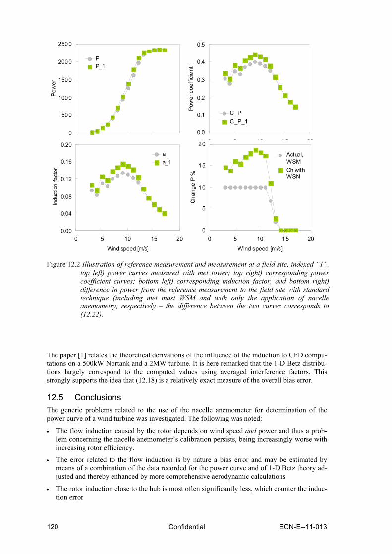
120 Confidential ECN-E--11-013
The paper [1] relates the theoretical derivations of the influence of the induction to CFD compu-tations on a 500kW Nortank and a 2MW turbine. It is here remarked that the 1-D Betz distribu-tions largely correspond to the computed values using averaged interference factors. This strongly supports the idea that (12.18) is a relatively exact measure of the overall bias error.
12.5 Conclusions The generic problems related to the use of the nacelle anemometer for determination of the power curve of a wind turbine was investigated. The following was noted:
• The flow induction caused by the rotor depends on wind speed and power and thus a prob-lem concerning the nacelle anemometer’s calibration persists, being increasingly worse with increasing rotor efficiency.
• The error related to the flow induction is by nature a bias error and may be estimated by means of a combination of the data recorded for the power curve and of 1-D Betz theory ad-justed and thereby enhanced by more comprehensive aerodynamic calculations
• The rotor induction close to the hub is most often significantly less, which counter the induc-tion error
0
500
1000
1500
2000
2500
0 5 10 15 20Wind speed [m/s]
Pow
erPP_1
0.00
0.04
0.08
0.12
0.16
0.20
0 5 10 15 20
Wind speed [m/s]
Indu
ction
facto
r
aa_1
0.0
0.1
0.2
0.3
0.4
0.5
0 5 10 15 20
Wind speed [m/s]
Pow
er c
oeffi
cien
t
C_PC_P_1
0
5
10
15
20
0 5 10 15 20
Wind speed [m/s]
Cha
nge
P %
Actual,WSMCh withWSN
Figure 12.2 Illustration of reference measurement and measurement at a field site, indexed “1”.
top left) power curves measured with met tower; top right) corresponding power coefficient curves; bottom left) corresponding induction factor, and bottom right) difference in power from the reference measurement to the field site with standard technique (including met mast WSM and with only the application of nacelle anemometry, respectively – the difference between the two curves corresponds to (12.22).

ECN-E--11-013 Confidential 121
• The radial transient in induction factor close to the hub – and therefore potentially close to the position of the nacelle anemometer – is high and may make it difficult to determine the error to be compensated for.
• In all, it is believed that nacelle anemometry is a viable option, given that careful investiga-tion of and correction for the error caused by induction is made in addition to the directions made in the present draft of the standard for nacelle anemometry power curve measurements.
12.6 References [1] Frandsen S, “The Generics of Wind Turbine Nacelle Anemometry”, EWEC2009 Mar-
seille
[2] Pedersen TF, "Trends in power performance measurement standards", AWEA'94
[3] Antoniou I, Pedersen TF, "Nacelle Anemometry on a 1MW Wind Turbine: Comparing the power performance results by use of the nacelle or mast anemometer", Risø-R-941(EN), August 1997
[4] Frandsen, S. (ed.); Antoniou, I.; Chaviaropoulos, T.; Dahlberg, J.A.; Derrick, A.; Douvi-kas, D.; Dunbabin, P.; Hansen, J.C.; Hunter, R.; Kanellopoulos, D.; Kapsalis, G.; Kristen-sen, L.; Aagaard Madsen, H.; Mortensen, N.G.; Ruffle, R., “Power performance assess-ment. Final report”. (Risø National Laboratory, Roskilde, 1999) 205 p
[5] Dahlberg, J.-A.; Frandsen, S.; Aagaard Madsen, H.; Antoniou, I.; Pedersen, T.F.; Hunter, R.; Klug, H., “Is the nacelle mounted anemometer an acceptable option in performance testing?”. In: Wind energy for the next millennium. Proceedings. 1999 European wind energy conference (EWEC '99), Nice (FR), 1-5 Mar 1999. Petersen, E.L.; Hjuler Jensen, P.; Rave, K.; Helm, P.; Ehmann, H. (eds.), (James and James Science Publishers, London, 1999) p. 624-627
[6] Dahlberg, J.-A.; Frandsen, S.; Aagaard Madsen, H.; Antoniou, I.; Pedersen, T.F.; Hunter, R.; Klug, H., “Is the nacelle mounted anemometer an acceptable option in performance testing?”. In: Wind energy for the next millennium. Proceedings. 1999 European wind energy conference (EWEC '99), Nice (FR), 1-5 Mar 1999. Petersen, E.L.; Hjuler Jensen, P.; Rave, K.; Helm, P.; Ehmann, H. (eds.), (James and James Science Publishers, London, 1999) p. 624-627
[7] Frandsen, S.; Antoniou, I.; Hansen, C.J.; Kristensen, L.; Aagaard Madsen, H.; Chaviaro-poulos, B.; Douvikas, D.; Dahlberg, J.A.; Derrick, A.; Dunbabin, P.; Hunter, R.; Ruffle, R.; Kanellopoulos, D.; Kapsalis, G., "Redefinition power curve for more accurate perfor-mance assessment of wind farms", Wind Energy (2000) 3 , 81-111
[8] Frandsen, S.; Antoniou, I.; Hansen, C.J.; Kristensen, L.; Aagaard Madsen, H.; Chavia-ropoulos, B.; Douvikas, D.; Dahlberg, J.A.; Derrick, A.; Dunbabin, P.; Hunter, R.; Ruffle, R.;
[9] Albers A, Klug H, Westermann D, "Power Performance Verification", EWEC'99
[10] Pedersen TF, et.al. "Spinner Anemometry - An Innovative Wind Measurement Concept", EWEC2007 Milan
[11] IEC CD 61400-12-2 “WIND TURBINES – Part 12-2: Power performance of electricity producing wind turbines based on nacelle anemometry”, 88/325/CD, 2008-07-18
[12] Betz, A. „Der Maximum der theoretisch möglichen Ausnützung des Windes durch Windmotoren“, 1920, Zeitschrift für das gesamte Turbinenwesen, Heft 26, Sept. 26, pp. 307-309

122 Confidential ECN-E--11-013

ECN-E--11-013 Confidential 123
13. Spinner anemometry as an alternative to nacelle anemometry
Troels Friis Pedersen
13.1 Introduction The state of the art of measuring wind on wind turbines is based on nacelle anemometry. In na-celle anemometry wind speed and wind direction are measured with sensors mounted on the up-per side of the nacelle behind the rotor. Typically the sensors comprise a redundant pair of cup anemometers and wind vanes or a couple of 2D sonic sensors, see Figure 13.1. Nacelle anemo-metry provides input to the control system for yaw control, for start up and shut down, and is also used for power performance verification. Meanwhile, nacelle anemometry is hampered by the fact that it is positioned behind the rotor [1]. Nacelle anemometry measures wind that is in-fluenced by: the wakes of the blade roots, the blade root vortices, the boundary layer over the nacelle, and the mounting arrangement of the nacelle anemometry. These effects can be cali-brated for to a certain extent, but nacelle anemometry is also dependent on accurate adjustment at mounting. If the effect is significant, as indicated in Figure 13.2, it leads to losses in electric power and increased loads.
Figure 13.1 Arrangement of nacelle anemometry on the back of the nacelle of modern wind turbines. The instruments are typically mounted on a reasonably solid support structure with lightning protection covering the instruments and with redundant mounting of instruments
Figure 13.2 Often seen in the landscape: wind turbines that deviate significantly in yawing direction
13.2 Wind measurement in front of the rotor With the so-called “spinner anemometer” the wind is measured on the wind turbine spinner in front of the rotor. Measurement of wind in front of the rotor avoids most of the flow distortion effects that is inherent in nacelle anemometry. Due to the rotation, the flow angle wind mea-
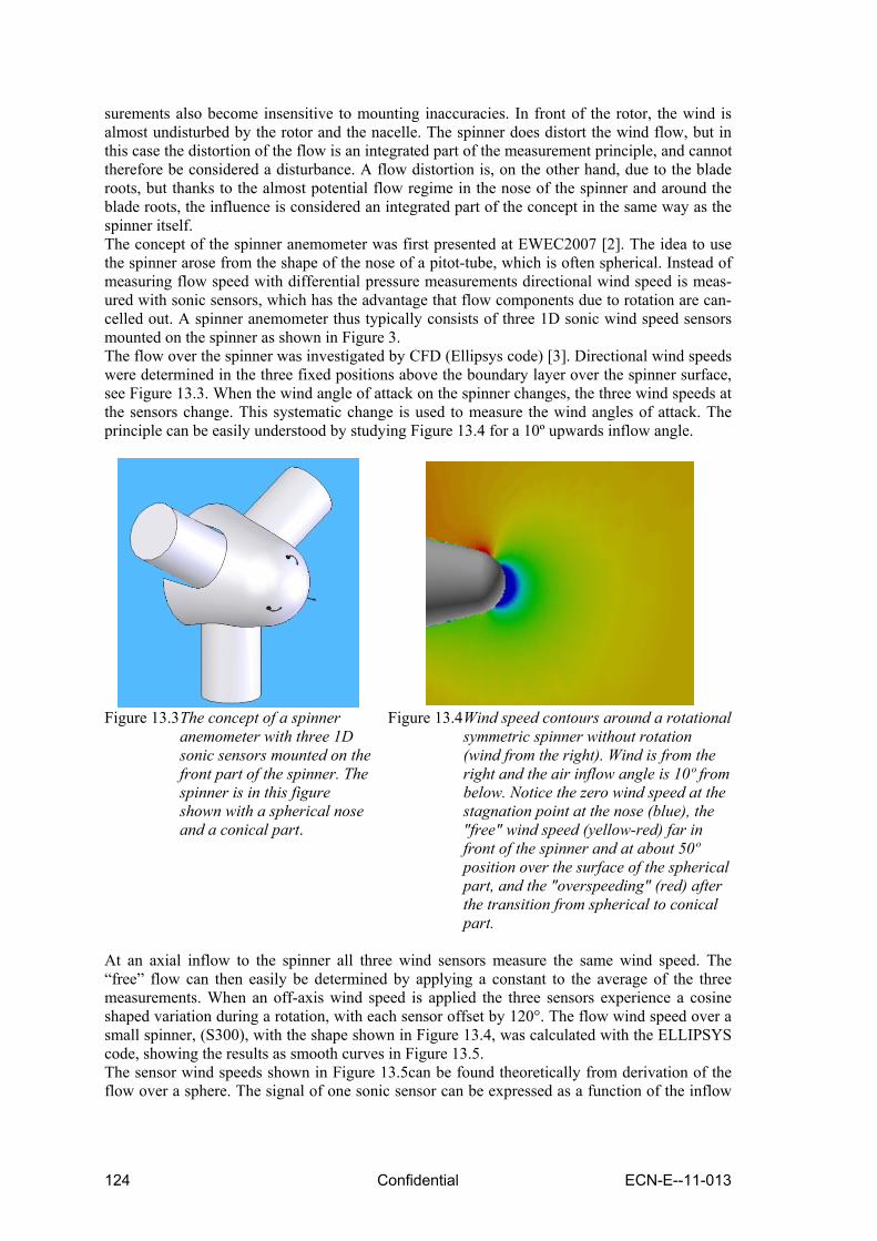
124 Confidential ECN-E--11-013
surements also become insensitive to mounting inaccuracies. In front of the rotor, the wind is almost undisturbed by the rotor and the nacelle. The spinner does distort the wind flow, but in this case the distortion of the flow is an integrated part of the measurement principle, and cannot therefore be considered a disturbance. A flow distortion is, on the other hand, due to the blade roots, but thanks to the almost potential flow regime in the nose of the spinner and around the blade roots, the influence is considered an integrated part of the concept in the same way as the spinner itself. The concept of the spinner anemometer was first presented at EWEC2007 [2]. The idea to use the spinner arose from the shape of the nose of a pitot-tube, which is often spherical. Instead of measuring flow speed with differential pressure measurements directional wind speed is meas-ured with sonic sensors, which has the advantage that flow components due to rotation are can-celled out. A spinner anemometer thus typically consists of three 1D sonic wind speed sensors mounted on the spinner as shown in Figure 3. The flow over the spinner was investigated by CFD (Ellipsys code) [3]. Directional wind speeds were determined in the three fixed positions above the boundary layer over the spinner surface, see Figure 13.3. When the wind angle of attack on the spinner changes, the three wind speeds at the sensors change. This systematic change is used to measure the wind angles of attack. The principle can be easily understood by studying Figure 13.4 for a 10º upwards inflow angle.
Figure 13.3 The concept of a spinner
anemometer with three 1D sonic sensors mounted on the front part of the spinner. The spinner is in this figure shown with a spherical nose and a conical part.
Figure 13.4 Wind speed contours around a rotational symmetric spinner without rotation (wind from the right). Wind is from the right and the air inflow angle is 10º from below. Notice the zero wind speed at the stagnation point at the nose (blue), the "free" wind speed (yellow-red) far in front of the spinner and at about 50º position over the surface of the spherical part, and the "overspeeding" (red) after the transition from spherical to conical part.
At an axial inflow to the spinner all three wind sensors measure the same wind speed. The “free” flow can then easily be determined by applying a constant to the average of the three measurements. When an off-axis wind speed is applied the three sensors experience a cosine shaped variation during a rotation, with each sensor offset by 120°. The flow wind speed over a small spinner, (S300), with the shape shown in Figure 13.4, was calculated with the ELLIPSYS code, showing the results as smooth curves in Figure 13.5. The sensor wind speeds shown in Figure 13.5can be found theoretically from derivation of the flow over a sphere. The signal of one sonic sensor can be expressed as a function of the inflow

ECN-E--11-013 Confidential 125
angle α and the inflow azimuth position φ at the location of the stagnation point on the spinner and the free wind speed U and two constants K1 and K2:
1 2( cos sin cos )SV U K Kα α ϕ= + ( 13.1 )
As seen in Figure 13.5, the average sensor wind speed over one rotation decreases with increas-ing inflow angle while the amplitude increases. In fact the average sensor wind speed is reduced with the cosine to the yaw setting angle while the amplitude increases with the sine. The ELLIPSYS calculated curves (smooth) in Figure 13.5 correspond very precisely to the theo-retical curves (open dots) up to inflow angles at 60°. Only at 80° there is a significant deviation. In fact the analysis shows that the deviations decrease with the inflow angle. This is a character-istic that is in line with the purpose of the instrument; the smaller the yaw error, the more accu-rate the yaw error measurement.
Sensor wind speeds S300 CFD
-6-4-202468
1012
0 60 120 180 240 300 360Azimuth (deg)
Sen
sor w
ind
spee
d (m
/s)
010203040608010(pot)20(pot)30(pot)40(pot)60(pot)80(pot)
aoa (deg)
Figure 13.5 ELLIPSYS computed velocity distribution around the S300 spinner for 10m/s off-
axis inflow at 0º, 10º, 20º, 30º, 40º, 60º, and 80º, smooth curves. Open dots represents theoretical values from formula 1.
With the expression in formula (13.1) for one sensor an expression can be found for each of the three sensors positioned at equidistant angles on the spherical nose. The inverse solution, to find the wind values from the sensor path air speeds, can then easily be derived. The yaw error and the flow inclination angle can be determined with only two instrument constants K1 and K2. K1 is mostly connected to determination of the wind speed and K2 is mostly connected to the flow angles. This makes calibration of the instrument just as simple as the gain and offset of a cup anemometer.
13.3 Free field comparison to 3D sonic anemometer The S300 spinner anemometer was tested under field conditions at the Risø test site using the simple spinner anemometer algorithm with two constants, and with a rotational speed of 15rpm. A 3D Gill Windmaster sonic anemometer was mounted at same height and about three meters to the side of the spinner anemometer. The spinner anemometer and the sonic anemometer are shown in Figure 13.6. Figure 13.7 to Figure 13.9 show 100 seconds of time traces of the two wind sensors. The two sensors signals show quite comparable results.

126 Confidential ECN-E--11-013
S300 with "new" sensors - Wind Speed
0
2
4
6
8
10
12
7000 7500 8000 8500 9000 9500 10000 10500Samples (35Hz)
U (m
/s)
SonicSpinner
Figure 13.6 Arrangement of the S300 spinner anemometer with "new" sensors in comparison with the sonic anemometer at Risø test site
Figure 13.7 Comparison of measured wind speed at 35Hz sampling rate (100sec of data) of spinner anemometer and 3D sonic anemometer
S300 with "new" sensors - Wind direction
-50-40-30-20-10
01020304050
7000 7500 8000 8500 9000 9500 10000 10500Samples (35Hz)
Wdr
(deg
)
SonicSpinner
S300 with "new" sensors - Flow inclination angle
-50-40-30-20-10
01020304050
7000 7500 8000 8500 9000 9500 10000 10500Samples (35Hz)
Incl
inat
ion
angl
e (d
eg) Sonic
Spinner
Figure 13.8 Comparison of measured horizontal inflow angle at 35Hz sampling rate
Figure 13.9 Comparison of measured vertical inflow angle at 35Hz sampling rate
13.4 Calibration of the spinner anemometer There have been developed calibration procedures for the spinner anemometer. The key calibra-tion factors of the spinner anemometer are the K1 and K2 factors, which are calibrated with a stopped rotor without rotor induction. The calibration can be made by CFD calculations or by field measurements. This calibration can be supplemented with an accredited traceable wind tunnel calibration and an internal spinner anemometer calibration to compensate for geometry deviations of the spinner and for sensor mounting.
13.5 Tests of spinner anemometers on wind turbines The spinner anemometer has been tested on a 3,6MW wind turbine [4, 5], see Figure 13.10. Yaw error measurements are shown in Figure 13.11. In this case the level of yaw error might lead to power losses in the order of 2%. The spinner anemometer has also been tested on tur-bines of different sizes.

ECN-E--11-013 Confidential 127
Yaw error versus wind speed (all sonic sensors)
-5
0
5
10
15
20
25
0 5 10 15 20 25Spinner anemometer wind speed (m/s)
Yaw
err
or (3
D) (
deg)
Figure 13.10 The three 1D sonic wind sensors mounted on the 3,6MW wind turbine spinner at Risø DTU Høvsøre test site.
Figure 13.11 Yaw error of 3,6MW wind turbine (10min averages).
Further work The spinner anemometer can be used for yawing of wind turbines, power performance verifica-tion, and for flow inclination measurements in complex terrain. A new project (EUDP Spinner-farm) has been started in 2009 which has the purpose to study yaw statistics of offshore wind turbines, to determine potential power losses due to yaw errors, and to verify power perfor-mance by nacelle/spinner anemometry.
13.6 Conclusions The idea of using the spinner of a wind turbine for wind measurements has been investigated theoretically and experimentally. A spinner anemometer with a small spinner has been investi-gated in detail by wind tunnel tests and CFD, and the investigations confirm the ideas of the wind measurement concept. Spinner anemometers were tested on a 3,6MW wind turbine, and on a number of other wind turbines of different size, and the tests confirm that yaw errors can be measured accurately, and that wind turbine yawing can be improved.
13.7 References [1] Frandsen S, Sørensen JN, Mikkelsen R, Pedersen TF, Antoniou I, Hansen K, 2009: The
generics of wind turbine nacelle anemometry, EWEC2008 Marseille
[2] Pedersen TF, Madsen HA, Møller R, Courtney M, 2007: Spinner anemometry – an inno-vative wind measurement concept, EWEC2007 Milan
[3] Pedersen TF, Sørensen NN, Enevoldsen P, 2008: Aerodynamics and characteristics of a spinner anemometer, The Science of Making Torque from Wind
[4] Pedersen TF, Vita L, Sørensen NN, Enevoldsen P, 2008: Operational experiences with a spinner anemometer on a MW size wind turbine, EWEC2008 Marseille

128 Confidential ECN-E--11-013

ECN-E--11-013 Confidential 129
14. Long term stability of cup anemometer operational character-istics
14.1 Identification of the problem Anemometer calibration is of fundamental importance for every wind energy related measure-ment activity. For this reason, international standardization bodies, apart from the usual metro-logical confirmation methodologies used in all measurement equipment (traceable calibration, proper maintenance, documented life long history) require additional measures for anemometers used in wind energy applications. The aim is to assure that any possible degradation of the op-erational characteristics of anemometers during their operational period is kept within known limits, to allow for a reliable estimation of the measurement uncertainty. Recalibration of the primary anemometers is proposed as the preferred method, while in-situ comparison is ac-cepted as a second solution. Detailed presentation of method used to approach the above problem and results obtained are given in [1] (recalibration) and [2] (insitu comparison). In the following main features from both studies are briefly presented.
14.2 Method of approach Recalibration The Laboratory for Wind Turbine Testing of CRES applies as a standard procedure the recali-bration of cup anemometers after operation in the field, a common practice among Testing Laboratories. A large data base of recalibrations of cup anemometers has evolved through the Laboratory’s operation in the last years. In the present work, statistical analysis of the differ-ences seen in the response characteristics of cup anemometers before and after their use is made. The differences were compared to the overall uncertainty of the calibration procedure, and the effect of operation duration was examined. The statistical analysis aims at providing a sound base for the decisions related to the determination of the recalibration interval of cup anemometers. To get a measurable value for the effect of usage on the operational characteristics, the differ-ence in wind velocity (DV) corresponding to the same frequency output as estimated from the calibration characteristics before (a1, b1) and after the use (a2, b2) is calculated, as in the fol-lowing equations
21 VVDV −= where
111 * bfaV +=
222 * bfaV += f selected frequency
α1, b1, response characteristics as defined by the calibration before use
α2, b2, response characteristics as defined by the calibration after use
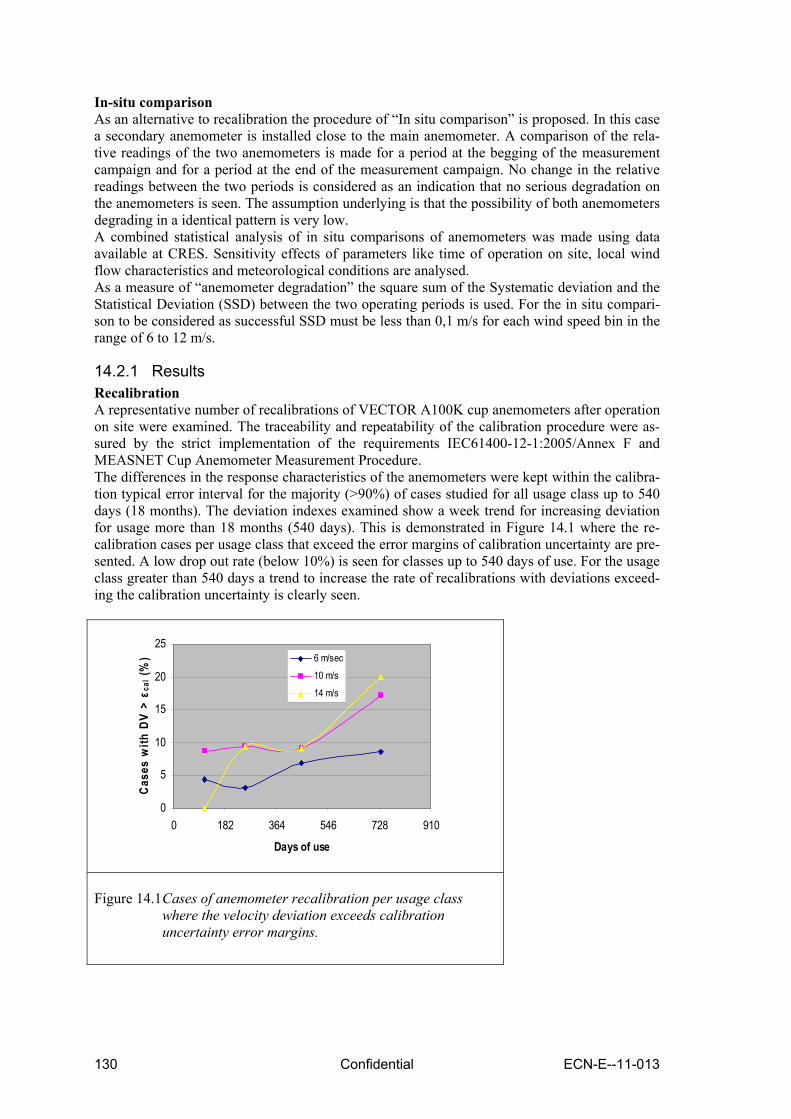
130 Confidential ECN-E--11-013
In-situ comparison As an alternative to recalibration the procedure of “In situ comparison” is proposed. In this case a secondary anemometer is installed close to the main anemometer. A comparison of the rela-tive readings of the two anemometers is made for a period at the begging of the measurement campaign and for a period at the end of the measurement campaign. No change in the relative readings between the two periods is considered as an indication that no serious degradation on the anemometers is seen. The assumption underlying is that the possibility of both anemometers degrading in a identical pattern is very low. A combined statistical analysis of in situ comparisons of anemometers was made using data available at CRES. Sensitivity effects of parameters like time of operation on site, local wind flow characteristics and meteorological conditions are analysed. As a measure of “anemometer degradation” the square sum of the Systematic deviation and the Statistical Deviation (SSD) between the two operating periods is used. For the in situ compari-son to be considered as successful SSD must be less than 0,1 m/s for each wind speed bin in the range of 6 to 12 m/s.
14.2.1 Results Recalibration A representative number of recalibrations of VECTOR A100K cup anemometers after operation on site were examined. The traceability and repeatability of the calibration procedure were as-sured by the strict implementation of the requirements IEC61400-12-1:2005/Annex F and MEASNET Cup Anemometer Measurement Procedure. The differences in the response characteristics of the anemometers were kept within the calibra-tion typical error interval for the majority (>90%) of cases studied for all usage class up to 540 days (18 months). The deviation indexes examined show a week trend for increasing deviation for usage more than 18 months (540 days). This is demonstrated in Figure 14.1 where the re-calibration cases per usage class that exceed the error margins of calibration uncertainty are pre-sented. A low drop out rate (below 10%) is seen for classes up to 540 days of use. For the usage class greater than 540 days a trend to increase the rate of recalibrations with deviations exceed-ing the calibration uncertainty is clearly seen.
0
5
10
15
20
25
0 182 364 546 728 910
Days of use
Case
s w
ith D
V >
εca
l (%
) 6 m/sec
10 m/s
14 m/s
Figure 14.1 Cases of anemometer recalibration per usage class
where the velocity deviation exceeds calibration uncertainty error margins.

ECN-E--11-013 Confidential 131
In-situ comparison A sensitivity analysis of the In situ comparison results, using as an index the SSD values esti-mated by the procedure was made. The operation time on site, the annual mean wind speed, the mean turbulence intensity and the annual mean temperature where examined.
00.02
0.040.06
0.080.1
0.12
0.140.16
0 200 400 600 800Days of use
SSD
(m/s
ec)
02
468
1012
1416
Sam
ples
per
bin
6 to 79 to 1011 to 12IEC61400-12-1Mean SSDSamples per bin
Figure 14.2 : Binned SSD values as a function of operation time on site (only cases with Vector A100 series ane-mometers) A weak dependence of averaged SSD values to operation time was seen (see Figure 14.2), as should be expected, since increased operation time on site may increase anemometer bearing wear. No obvious effect on SSD from site annual mean wind speed, mean turbulence intensity, and mean air temperature were detected for the range of the parameters covered. In situ comparison was successful for 90% of cases examined. Acceptable results where found even for anemometers operating more than 18 month on site. Where available, recalibrations of anemometers in the wind tunnel after the end of the measurement campaign, were in full accor-dance with in situ results.
14.2.2 Discussion The differences in the response characteristics of the anemometers are kept within the calibra-tion typical error interval for the majority (>90%) of cases studied for all usage class up to one year, while, of the limited data available in higher usage classes (up to 18 months) similar trend is observed. The above is confirmed by both methods applied (recalibration of anemometers af-ter use and in-situ comparison). The above results suggest that, at least for the type of instruments mainly examined in the pre-sent study ( VECTOR A100K series anemometers) the calibration interval could be increased up to 18 months with out affecting the reliability or the uncertainty of the measurements. Additionally, the good agreement in the results of both recalibration and in-situ comparisons support the position that the “in situ comparison” as described in IEC 61400-12-1:2005 provides a reliable tool for the verification of anemometer calibration integrity. Further work on the effect of anemometer type, and operating conditions – temperature range, air salinity, and dust etc- could provide important information to the manufacturers and users of cup anemometers that could help in improve the reliability of wind speed measurements.

132 Confidential ECN-E--11-013
14.3 Applicability of current power performance measurement recom-mended practices in various types of terrains.
14.3.1 Identification of the problem During the first years of the wind power expansion in Europe, the easily accessible flat terrain sites with good wind potential were the first to be developed in the wind pioneering countries such as Denmark, Holland, and Northern states of Germany. Wind turbines today can be seen operating all over the world in various terrain types. Since the power performance verification is considered a vital tool in the development of an efficient wind farm, an intense discussion is un-der way, considering how reliable power performance verification measurements are in complex terrain sites are. Spatial variations in wind speed (terrain induced distortion in the flow field, wind shear), flow inclination relative to the wind turbine rotor, and large differences in air den-sity are some of the parameters that are pointed out as having an effect on the power perform-ance of a wind turbine operating in complex terrain sites. Considerable efforts by both the scientific community and the industry have been made to as-sess the above issues, but the actual physical problem is not yet addressed in full. Furthermore the urgent need to have workable tools to make power performance verification in complex ter-rain sites, have led standardization organizations and expertise networks (namely IEA, IEC and MEASNET) to include in their recommendations special guidelines aiming at reducing uncer-tainties associated to complex terrain sites.
14.3.2 Method of approach Some sample cases of power curve verification of passive and active power control wind tur-bines w/t operating in various terrains (from semi-flat to very complex) were examined. It should be note that the machine examined were in the low to medium range with nominal power 500 kW to 1.5 MW) and with rotor diameters from 50 to 70 m. The difference between the Annual Energy Production (AEP) measured in the actual sites com-pared to the guaranteed AEP (∆AEP) was used as a measure of terrain dependency of the power performance of a wind turbine and therefore as an index for the suitability of the recommended procedures in various terrains. A sensitivity analysis, using the ∆AEP as an index, was made for some of the parameters ex-pected to influence the power performance (magnitude of site calibration correction factors, tur-bulence intensity, distance of reference mast, air density, etc). Detailed presentations of the analysis, methods and results were presented in [3].
14.3.3 Results and discussion The available results from the comparison of the power performance characteristics measured in complex terrain compared to flat terrain, in general supports the suitability of the methods pro-posed for medium sized wind turbines, and also underlines the influence of both terrain and ma-chine related parameters in the uncertainty of the measurement results. Deviations from the warranted power curve were within the typical error of measurement, and comparable to overall statistical scatter seen in the AEP of wind turbines operating in flat terrain.. Possible correlations between parameters characterizing the flow field in complex terrain sites and the deviations from the warranted AEP were subsequently investigated. The effect of the terrain on the evolution of the wind flow around the wind turbines was evident in all cases, as quantified by the impact of altitude difference between the reference mast and WT on the site calibration correction factors, by wide variations in shear profiles, as well as the differences in the site mean air density. A sensitivity analysis, using the ∆AEP as an index, showed small de-pendence of ∆AEP to increasing site calibration correction factors, as also to increasing direc-tional sensitivity of the site calibration factors and turbulence levels. No effect was observed for other parameters such as terrain inclination, distance of reference mast from the WT, air density difference, sector width etc. Considering this, the differences in ∆ΑΕP are smaller than the es-timated measurement error, hence it can be concluded that the application of the current proce-
ECN-E--11-013 Confidential 133
dures successfully reduced the influence of complex terrain parameters on the results for both pitch and stall regulated medium sized wind turbines. Some weaknesses of the site calibration procedure proposed, especially in very complex terrain are revealed. Current standards propose the use of a unified correction factor for a very wide wind speed range (4-16m/s). As it is proved in the present work [3], this procedure works very well in most cases, but can lead to additional errors in extreme cases, since in very complex ter-rain sites, the flow field strongly depends on the wind speed magnitude. The above further stresses the importance of a thorough verification of site calibration results. Shear profiles were also examined in some of the sample cases. The analysis of the shear pro-files revealed a wide variation of profiles among the cases studied, while strong direction de-pendence was also seen in some of the cases. More detailed parametric analysis of shear effect on the power curve is necessary. As the above approach showed, for medium, sized wind turbines, the application of the current recommended procedures, the power performance of WTs in various terrains can be success-fully evaluated and produce coherent and accurate results.
14.4 Definition of reference wind speed for power curve measurements of large wind turbines (>2.0 MW).
14.4.1 Identification of the problem Modern wind-industry history has shown a constant trend towards the development of signifi-cantly larger, not only in hub height (Hhub), but also in rotor diameter, Multi-MW Wind Tur-bines (WTs). At the same time, power performance tests are being implemented by measuring the wind speed at Hhub assuming that the wind speed is uniform over the rotor area. This is a fair assumption as far as small scale WTs are concerned, while being by far simplistic for the large scale ones. Wind speed, turbulence and wind direction do vary with height, in respect to the me-teorological regime and / or the terrain morphology. Consequently, the uncertainty related to the representative wind speed is increased, affecting the reliability of power performance and load predictions. The evaluation of the wind speed in over the whole rotor area is an issue open since a long time.
14.4.2 Method of approach Sample power curve measurement campaigns, meeting the IEC 614000-12-1:2005 requirements are examined involving wind turbines with nominal power output in the range of 800 - 1500 kW and operating in a variety of terrain types, from semi flat terrain to highly complex terrain. Ad-ditionally to the current standard requirements, wind speed was measured at heights below hub height also, allowing the wind shear to be estimated. On two of the cases studied, power curve data were analysed applying a new definition for the reference wind speed as proposed by An-toniou et all in [5]. The swept area of the rotor is divided to eight horizontal zones, assuming constant wind speed along each zone and the energy flux through each “constant speed zone” is calculated. The “equivalent wind speed” is defined as the wind speed giving the same total energy flux, as the sum of the energy fluxes by each “constant speed zone”, as detailed in Equation (14.1), where
iU is the wind speed along i-th “constant speed zone” and Ai the area of the i-th “constant speed zone” and A the rotor’s swept area.
iieqM AUA
U ⋅⋅= ∑11 ( 14.1 )

134 Confidential ECN-E--11-013
If turbulence is taken into account then the equation giving the equivalent wind speed 1eqTU be-
comes,
iieqT AUA
U ⋅⋅= ∑ 3 31
1 ( 14.2 )
where, 3iU is the average energy flux defined as,
( )23
2
233 3131 TIUU
UU +⋅=⎟⎟⎠
⎞⎜⎜⎝
⎛+⋅=
σ ( 14.3 )
where σ is the standard deviation and IT is turbulence intensity.
Differently, the equivalent wind speed can be expressed as the wind speed which results in the same energy flux through the rotor area as the varying wind speed over the integration period.
( )3 33
1 ∑ ⋅⋅= iieqT AUA
U ( 14.4 )
Direct measurement of wind speed at the complete rotor area requires either a mast high enough to reach upper blade tip position or a lower mast in combination with remote sensing systems (Lidar or Sodar). Both configurations are well in excess of the budget of a typical commercial power curve verification campaign. As a less expensive alternative, conventional masts used for site calibration and power curve campaigns were equipped with additional anemometers at two to four levels below hub. This configuration gives instantaneous velocity measurements at vari-ous heights up to Hhub allowing the estimation of shear profiles. Thereupon, the wind speed along the rotor surface can be estimated, based on the assumption that the shear profile in the upper half of the rotor is same as the one below. This assumption is definitely a drawback of this approach, since discontinuity in the shear profiles has been observed in various cases. On the other hand, such an approach allows the use of data from conventional measurement cam-paigns in complex terrain with the view to investigating alternative methods for the definition of the reference wind speed. For the estimated wind shear profile, total energy flux through the rotor is calculated, and an equivalent uniform wind speed value is defined. The measured power curves derived when us-ing the “hub-height wind speed” and the “equivalent wind speed” are compared to the warranted power curves, with the aim of evaluating whether this approach improves measurement reliabil-ity. Additionally on one of the cases, short term wind speed shear measurements were being ob-tained using a Lidar system and were compared with these of an adjacent met mast equipped with cup anemometers. Detailed description of the approach followed and of the results obtained were presented in [4].
14.4.3 Results and discussion Data from sample cases involving commercial power performance measurements in complex terrain sites were analysed. Alternative method for the definition of the reference wind speed involving an “equivalent rotor averaged wind speed” as described above was applied. The wind

ECN-E--11-013 Confidential 135
speed shear along the rotor disk was estimated using cup anemometer measurements corre-sponding to heights at the lower part of the rotor. In the following graphs (Figure 14.3), results from one of the cases studied are presented. Differences in the power curve and AEP when using different definitions for the reference wind speed are given. Small differences between conventional Hhub wind speed and “rotor averaged wind speed” were observed. Assuming the local wind speed at each rotor “constant speed zone” to be proportional to the area of the zone, the zones close to hub were over- weighted (having larger area due to the fragments’ width) relative to the outer zones. On the outer constant speed zones, the torque increment for a given wind speed is larger than for an inner segment (closer to hub) due to the larger torque arm (distance of zone to the axis of rotor rotation. This effect is not weighted in the approach followed.
Power Curves ComparisonCase 2
-0.2
0
0.2
0.4
0.6
0.8
1
1.2
0 0.25 0.5 0.75 1 1.25 1.5U/Unom
P/P n
om WARRANTEDIEC31400-12-1UeqM1UeqT1UeqT3
(a)
Power Estimation Difference From Warranted Comparison / Case 2
-0.100-0.075-0.050-0.0250.0000.0250.0500.0750.100
0 0.2 0.4 0.6 0.8 1 1.2 1.4
U/Unom
ΔP/
Pno
mIEC61400-12-1UeqM1UeqT1UeqT3
(b)
Uncertainty A ComparisonCase 2
0.000
0.002
0.004
0.006
0.008
0.010
-0.1 0 0.1 0.2 0.3 0.4 0.5 0.6 0.7P/Pnom
s/P n
om
IEC31400-12-1UeqM1UeqT1UeqT3
(c)
AEP COMPARISONCase 2
0.8
0.9
1
1.1
0 0.25 0.5 0.75 1Umean/Unom
AEP
-E/A
EP-E
WA
RR
AN
TED
IEC61400-12-1UeqM1UeqT1UeqT3
(d)
Figure 14.3 CASE 2: Effect of Reference Wind Speed Definition on Power Curve
(a) P-U Curves (b) Difference from Warranted (c) Type A Uncertainty (d) AEP comparison
Still the differences between the Hhub wind speed and rotor averaged wind speed are small either seen as average power output or as Type A uncertainty in the binning procedure or as differ-ences in the AEP. Therefore, in the cases studied which correspond to small to medium sized wind turbines (hub height 45 to 70m) and operating in areas with smooth and predictable shear profiles (low exponent coefficients), the conventional definition of reference wind speed (hub height point measured) fits well with the rotor averaged definition for UeqM1, without turbu-lence. In all cases studied, the inclusion of turbulence term in the definition of the “rotor aver-aged wind speed”, gives small but non-negligible difference to the IEC calculations and war-ranted. The above demonstrates the fact that, due to rotor size not all turbulent fluctuations sensed by a cup anemometer, can be converted to useful energy by a wind turbine rotor.

136 Confidential ECN-E--11-013
The cases studied in the present work are limited compared to the variety of operating condi-tions found in complex terrain sites. Additional cases should be analysed covering a wider range of operating conditions, focusing in sites with steep wind shear, i.e. where the IT is rather low and wind speed stratification is noteworthy. However, provided the findings of the present analysis are verified at other cases as well, this could support the use of a test configuration with hub height mast and shear measuring anemometers for power performance measurements using alternative definition of the reference wind speed. This could serve as a less expensive alterna-tive to “blade tip tall towers” or remote sensing systems (such as Lidars) for short to medium wind turbines. A combination of short term operation of remote sensing systems with hub-height masts equipped with shear measuring anemometers could also be used for taller wind turbines, in combination with better monitoring of boundary layer stability conditions (temperature stratifi-cation etc).
14.5 Actions taken – improvements –response of wind energy commu-nity:
Anemometer recalibration interval
The Greek Accreditation organization, responsible for the accreditation of testing and meas-urements Laboratories (ESYD S.A ), confirmed the acceptance of 18 months as recalibration interval for anemometers used in wind energy applications (http://www.esyd.gr/pweb/s/20/files/kanonismoi/kritiriaOdigies/KO_AIOLIKO.pdf, in Greek) . Power performance measurements MEASNET Network issued a new recommendation for Power performance Measurements (MEASNET Procedure “Power performance measurements “, Ver 5,2009, http://www.measnet.com/power5.pdf). In this procedure, it is recommended to include wind shear data in the documentation of each power curve measurement campaign.
14.6 References [1]. Stefanatos N., Papadopoulos P., Binopoulos E., Kostakos A., Spyridakis G., "Effects of
long term operation on the performance characteristics of cup anemometers” Proc. Of EWEC 2007, Milan
[2]. Stefanatos N., Papadopoulos P., “Verification of anemometer calibrations“, Proc. of EWEC 2010, Warsaw
[3]. Stefanatos N., Mouzakis F., Binopoulos E., Kokkalidis F., Papadopoulos P. "Verification of power performance of active power control wind turbines in complex terrain” Proc. Of EWEC 2006, Athens
[4]. Stefanatos N., Zigras D., Foussekis D., Kokkalidis F., Papadopoulos P., Binopoulos E., "Revising reference wind speed definition for power performance measurements of multi-mw wind turbines” Proc. of EWEC 2008, Brussels.
[5]. Ioannis Antoniou et al. “Influence of Wind Characteristics on Turbine Performance” EWEC2007, Milan, Italy

ECN-E--11-013 Confidential 137
Appendix A Aerodynamics & Aero-elastics, Rotor structures Materials, and Turbine Foundations
Table A.1 List of parameters for WP2 Aerodynamics & Aero-elastics, WP3 Rotor structures and materials and WP4 Turbine Foundations
Param No
Parameter / Sig-nal Unit
Desired Ac-curacy (Un-certainty)
Trace-able (Y/N)
Sampling frequency range [Hz] (1)
Required / Optional Measurement position
WP2
and
WP3
Tur
bine
M
onito
ring
Farm
Mon
itorin
g
WP4
Des
ign
code
ver
i-fic
atio
n
WP4
Adv
ance
d C
ontr
ol
stra
tegi
es
1 Displacements (2) m To be deter-mined Y
It should be 8 times larger than the highest frequency to be studied
O
Blade, hub, tower, na-celle, substructure, foundation and individ-ual components
X X X X
1 Velocities (3) m/s To be deter-mined Y
It should be 8 times larger than the highest frequency to be studied
O
Blade, hub, tower, na-celle, substructure, foundation and individ-ual components
X X X X
1 Accelerations (4) m/s2 To be deter-mined Y
It should be 8 times larger than the highest frequency to be studied
O
Blade, hub, tower, na-celle, substructure, foundation and individ-ual components
X X X X
1 Nacelle accelera-tion in three direc-tions (5)
m/s2 0.05 m/s2 Y It should be 8 times
larger than the highest frequency to be studied
R
Nacelle, measurement in more locations to capture all degrees of freedom
X X X
1
Tower bending moment on differ-ent height levels (fore-aft, side-side and torsional)
kNm 3% Y It should be 8 times
larger than the highest frequency to be studied
R Tower X X X
1
Tower acceleration in three directions on different height levels
m/s2 0.05 m/s2 Y It should be 8 times
larger than the highest frequency to be studied
R Tower X X X
1
Substructure (mo-nopile, tripod, floating) bending moment on differ-ent height levels above and below mudline (fore-aft, side-side and tor-sional if relevant)
kNm 3% Y It should be 8 times
larger than the highest frequency to be studied
R Substructure X X X
1 Yaw moment kNm Target 3% Y It should be 8 times
larger than the highest frequency to be studied
R
Nacelle, it could be measured from the ro-tating structure, or from the fixed structure.
X X X
1 Tilt moment kNm 3% Y It should be 8 times
larger than the highest frequency to be studied
R
Nacelle, it could be measured from the ro-tating structure, or from the fixed structure.
X X X
1 Main shaft bending (0° 90°) kNm 3% Y
It should be 8 times larger than the highest frequency to be studied
R Main shaft X X X
1 Main shaft torsion kNm 3% Y It should be 8 times
larger than the highest frequency to be studied
R Main shaft X X X
1
Strain distribution to determine local stress distributions and for instance shear (anywhere)
kN 3% Y It should be 8 times
larger than the highest frequency to be studied
R
Blade, hub, tower, na-celle, substructure, foundation and individ-ual components
X
1
Blade bending moment along the blade length (flap-wise and edge-wise)
kNm 3% Y It should be 8 times
larger than the highest frequency to be studied
R Blade X X
1 Blade root bending moment (in-plane and out-of-plane)
kNm
Derived from blade bend-ing moments and pitch an-
gles
- - - X X X X
1 Blade torsional moment along the blade
kNm 3% Y It should be 8 times
larger than the highest frequency to be studied
R Blade X X
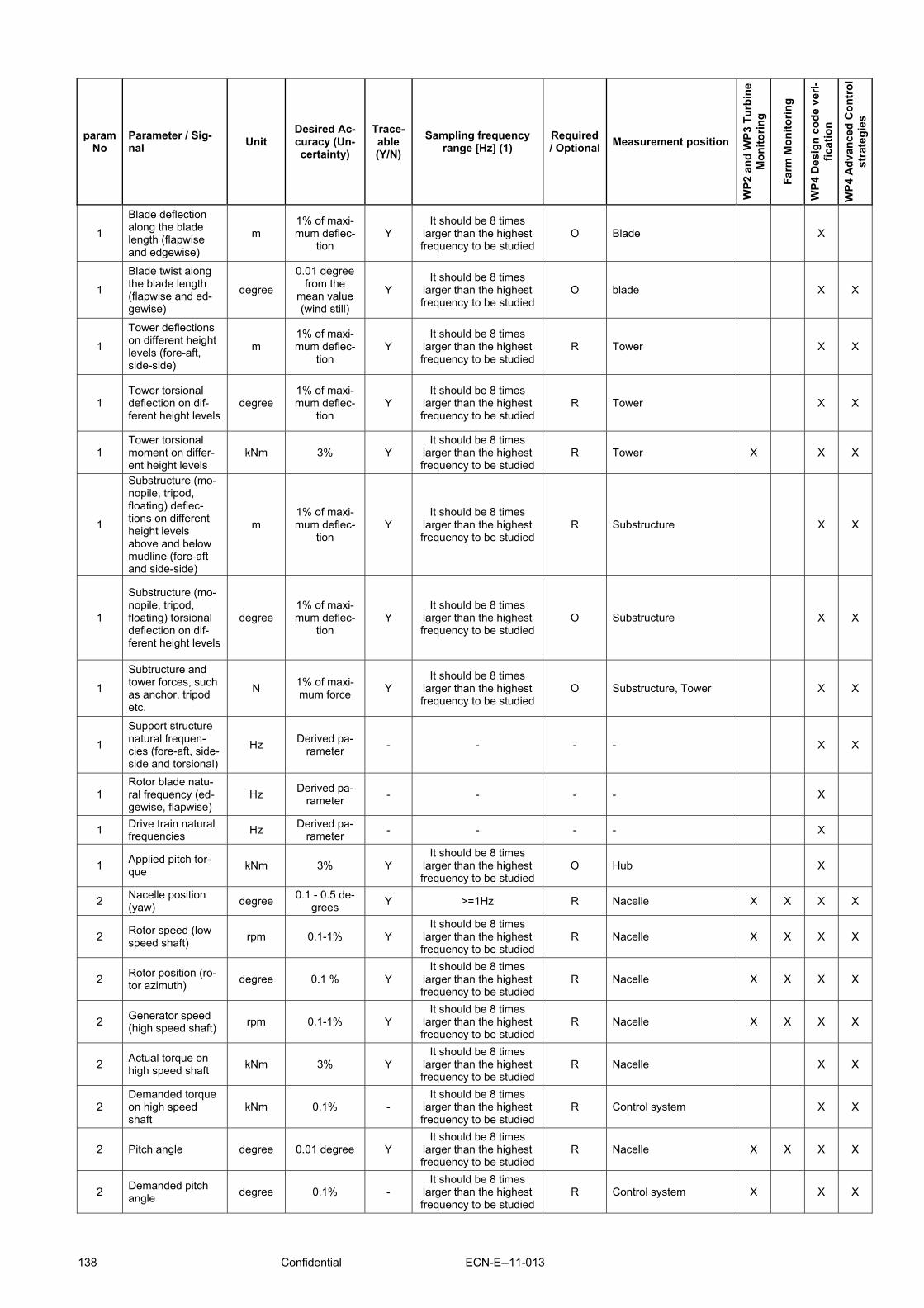
138 Confidential ECN-E--11-013
param No
Parameter / Sig-nal Unit
Desired Ac-curacy (Un-certainty)
Trace-able (Y/N)
Sampling frequency range [Hz] (1)
Required / Optional Measurement position
WP2
and
WP3
Tur
bine
M
onito
ring
Farm
Mon
itorin
g
WP4
Des
ign
code
ver
i-fic
atio
n
WP4
Adv
ance
d C
ontr
ol
stra
tegi
es
1
Blade deflection along the blade length (flapwise and edgewise)
m 1% of maxi-mum deflec-
tion Y
It should be 8 times larger than the highest frequency to be studied
O Blade X
1
Blade twist along the blade length (flapwise and ed-gewise)
degree
0.01 degree from the
mean value (wind still)
Y It should be 8 times
larger than the highest frequency to be studied
O blade X X
1
Tower deflections on different height levels (fore-aft, side-side)
m 1% of maxi-mum deflec-
tion Y
It should be 8 times larger than the highest frequency to be studied
R Tower X X
1 Tower torsional deflection on dif-ferent height levels
degree 1% of maxi-mum deflec-
tion Y
It should be 8 times larger than the highest frequency to be studied
R Tower X X
1 Tower torsional moment on differ-ent height levels
kNm 3% Y It should be 8 times
larger than the highest frequency to be studied
R Tower X X X
1
Substructure (mo-nopile, tripod, floating) deflec-tions on different height levels above and below mudline (fore-aft and side-side)
m 1% of maxi-mum deflec-
tion Y
It should be 8 times larger than the highest frequency to be studied
R Substructure X X
1
Substructure (mo-nopile, tripod, floating) torsional deflection on dif-ferent height levels
degree 1% of maxi-mum deflec-
tion Y
It should be 8 times larger than the highest frequency to be studied
O Substructure X X
1
Subtructure and tower forces, such as anchor, tripod etc.
N 1% of maxi-mum force Y
It should be 8 times larger than the highest frequency to be studied
O Substructure, Tower X X
1
Support structure natural frequen-cies (fore-aft, side-side and torsional)
Hz Derived pa-rameter - - - - X X
1 Rotor blade natu-ral frequency (ed-gewise, flapwise)
Hz Derived pa-rameter - - - - X
1 Drive train natural frequencies Hz Derived pa-
rameter - - - - X
1 Applied pitch tor-que kNm 3% Y
It should be 8 times larger than the highest frequency to be studied
O Hub X
2 Nacelle position (yaw) degree 0.1 - 0.5 de-
grees Y >=1Hz R Nacelle X X X X
2 Rotor speed (low speed shaft) rpm 0.1-1% Y
It should be 8 times larger than the highest frequency to be studied
R Nacelle X X X X
2 Rotor position (ro-tor azimuth) degree 0.1 % Y
It should be 8 times larger than the highest frequency to be studied
R Nacelle X X X X
2 Generator speed (high speed shaft) rpm 0.1-1% Y
It should be 8 times larger than the highest frequency to be studied
R Nacelle X X X X
2 Actual torque on high speed shaft kNm 3% Y
It should be 8 times larger than the highest frequency to be studied
R Nacelle X X
2 Demanded torque on high speed shaft
kNm 0.1% - It should be 8 times
larger than the highest frequency to be studied
R Control system X X
2 Pitch angle degree 0.01 degree Y It should be 8 times
larger than the highest frequency to be studied
R Nacelle X X X X
2 Demanded pitch angle degree 0.1% -
It should be 8 times larger than the highest frequency to be studied
R Control system X X X

ECN-E--11-013 Confidential 139
Param No
Parameter / Sig-nal Unit
Desired Ac-curacy (Un-certainty)
Trace-able (Y/N)
Sampling frequency range [Hz] (1)
Required / Optional Measurement position
WP2
and
WP3
Tur
bine
M
onito
ring
Farm
Mon
itorin
g
WP4
Des
ign
code
ver
i-fic
atio
n
WP4
Adv
ance
d C
ontr
ol
stra
tegi
es
2 Pitch rate degree/s Derived sig-nal X X X
2 Active electrical power kW 0.5% Y
It should be 8 times larger than the highest frequency to be studied
R
Between wind turbine and electrical connec-tion; It could be at dif-ferent locations, such as stator, rotor etc.
X X X X
2 Reactive electrical power kW 0.5% Y
It should be 8 times larger than the highest frequency to be studied
O
Between wind turbine and electrical connec-tion; It could be at dif-ferent locations, such as stator, rotor etc.
X X X X
2 Controller mode - Derived from controller Y
It should be 8 times larger than the highest frequency to be studied
R Control system X X X X
2 Availability - Derived from controller Y
It should be 8 times larger than the highest frequency to be studied
O X X X X
2 Failure - Derived from controller Y
It should be 8 times larger than the highest frequency to be studied
O X X X
2 Status - Derived from controller Y
It should be 8 times larger than the highest frequency to be studied
R Control system X X X
2 Wind speed measured at na-celle
m/s 0.1 m/s Y >=1Hz R Nacelle X X X X
2 Wind direction measured at na-celle
degree 1 degree Y >=1Hz R Nacelle X X X X
3
Wind speed at dif-ferent positions in the rotor plane (longitudinal, later-al and vertical)
m/s 0.1 - 0.25 m/s at 10 m/s Y >=1Hz R Rotor plane, free sector X X X X
3 Wind direction at different positions in the rotor plane
degree 2-5 deg Y >=1Hz R Rotor plane, free sector X X
3 Air Temperature oC 0.5-3 oC Y >=1Hz R Hub height X
3 Atmospheric pres-sure hPa 5 hPa Y >=1Hz R Hub height X
4 Sea surface eleva-tion m 0.1 m Y >=1Hz R Sea level X
4 Wave direction degree 5 degree Y >=1Hz R Sea level X
4 Current speed pro-file m/s 0.1 m/s Y >= 0.1Hz R From mudline til sea
level X
4 Current direction degree 5 degree Y >= 0.1Hz R From mudline til sea level X
4 Ice parameters (thickness) m 0.01m Y daily, hourly values O Sea level X X
4 Water temperature (6)
oC 0.3 degree C Y >=1Hz R Surface temperature X
5 Soil strata - Soil description as function of depth
- - Y once, or larger than 1/year R Soil X X
5 Internal friction angle of soil degree 5 degree Y once, or larger than
1/year R Soil X X
5 Cohesive strength kN/m2 ? Y once, or larger than 1/year ? Soil X X
5 Unit weight kN/m3 ? Y once, or larger than 1/year ? Soil X X
5 Scour ? ? Y once, or larger than 1/year ? Soil X X
5 Sea bed move-ment ? ? Y > 8 times the highest
frequency to be studied ? Soil X X
(1) For many parameters, it is noted that the sample frequency should be 8 times larger than the highest frequency to be studied. This is most practical, since the parameters could be used for more purposes with own requirements.
(2) Displacements. Examples are gearbox displacements, angular displacements of flexible coupling, etc (3) Velocities. Examples are pitch piston velocities, main shaft velocities etc. (4) Acceleration. Examples are accelerations in subcomponents etc. (5) The accelerometer should be applicable also for the lower frequencies encountered in larger wind turbines (6) Water temperature is included for stability of the atmospheric boundary layer In the future, the calibration by means of adding force on the turbine can be impossible, so new calibration methods should be defined

140 Confidential ECN-E--11-013
Appendix B Control systems and Condition Monitoring
Table B.1 List of parameters for WP5 Control systems and WP7 Condition Monitoring
Param No
Parameter / Sig-nal Unit
Desired Ac-curacy (Un-certainty)
Trace-able (Y/N)
Sampling frequency range [Hz] (1)
Required / Optional
Measurement posi-tion
WP5
Ope
ratio
nal
Con
trol
Sys
tem
s
WP5
Dev
elop
men
t of
Con
trol
str
ateg
ies
WP7
Con
ditio
n M
onito
ring
1 Displacements (2) m To be deter-mined Y
It should be 8 times larger than the highest frequency to be studied
O
Blade, hub, tower, na-celle, substructure, foundation and indi-vidual components. (8)
X X X
1 Velocities (3) m/s To be deter-mined Y
It should be 8 times larger than the highest frequency to be studied
O
Blade, hub, tower, na-celle, substructure, foundation and indi-vidual components
X X X
1 Accelerations (4) m/s2 To be deter-mined Y
It should be 8 times larger than the highest frequency to be studied
O
Blade, hub, tower, na-celle, substructure, foundation and indi-vidual components (9)
X X X (7)
1 Temperatures C To be deter-mined Y
It should be 8 times larger than the highest frequency to be studied
O Individual components X X X
1 Pressure Pa To be deter-mined Y
It should be 8 times larger than the highest frequency to be studied
O Individual components X X X
1 Liquid levels m To be deter-mined Y
It should be 8 times larger than the highest frequency to be studied
O Individual components X X X
1 Strain microstrain To be deter-mined Y
It should be 8 times larger than the highest frequency to be studied
O Individual components X X
1 Nacelle accelera-tion in three direc-tions
m/s2 0.05 m/s2 Y It should be 8 times
larger than the highest frequency to be studied
R
Nacelle, measurement in more locations to capture all degrees of freedom
X X X
1
Tower accelera-tion in three direc-tions on different height levels
m/s2 0.05 m/s2 Y It should be 8 times
larger than the highest frequency to be studied
R Tower X X X
1 Yaw moment kNm Target 3% Y It should be 8 times
larger than the highest frequency to be studied
O
Nacelle, it could be measured from the rotating structure, or from the fixed struc-ture.
X X X
1 Tilt moment kNm 3% Y It should be 8 times
larger than the highest frequency to be studied
O
Nacelle, it could be measured from the rotating structure, or from the fixed struc-ture.
X X X
1 Main shaft bend-ing (0° 90°) kNm 3% Y
It should be 8 times larger than the highest frequency to be studied
O Main shaft X X X
1 Main shaft torsion kNm 3% Y It should be 8 times
larger than the highest frequency to be studied
O Main shaft X X X
1
Blade bending moment along the blade length (flapwise and ed-gewise)
kNm 3% Y It should be 8 times
larger than the highest frequency to be studied
O Blade X X X
1
Blade root bend-ing moment (in-plane and out-of-plane)
kNm
Derived from blade bend-ing moments and pitch an-
gles
- - - - X X X
1 Blade torsional moment along the blade
kNm 3% Y It should be 8 times
larger than the highest frequency to be studied
O Blade X X
1
Blade deflection along the blade length (flapwise and edgewise)
m 1% of maxi-mum deflec-
tion Y
It should be 8 times larger than the highest frequency to be studied
O Blade X X

ECN-E--11-013 Confidential 141
param No
Parameter / Sig-nal Unit
Desired Ac-curacy (Un-certainty)
Trace-able (Y/N)
Sampling frequency range [Hz] (1)
Required / Optional
Measurement posi-tion
WP5
Ope
ratio
nal
Con
trol
Sys
tem
s
WP5
Dev
elop
men
t of
Con
trol
str
ateg
ies
WP7
Con
ditio
n M
onito
ring
1
Blade twist along the blade length (flapwise and ed-gewise)
degree
0.01 degree from the
mean value (wind still)
Y It should be 8 times
larger than the highest frequency to be studied
O Blade X X
1
Tower deflections on different height levels (fore-aft, side-side)
m 1% of maxi-mum deflec-
tion Y
It should be 8 times larger than the highest frequency to be studied
O Tower X X
1
Tower torsional deflection on dif-ferent height le-vels
degree 1% of maxi-mum deflec-
tion Y
It should be 8 times larger than the highest frequency to be studied
O Tower X X
1 Tower-top accele-rations (horizon-tal)
m/s2 to be deter-mined Y
It should be 8 times larger than the highest frequency to be studied
O Tower X X
1
Substructure and tower forces, such as anchor, tripod etc.
N 1% of maxi-mum force Y
It should be 8 times larger than the highest frequency to be studied
O Substructure, Tower X X
1
Support structure natural frequen-cies (fore-aft, side-side and tor-sional)
Hz Derived pa-rameter - - O - X X X
1 Rotor blade natu-ral frequency (ed-gewise, flapwise)
Hz Derived pa-rameter - - O - X X X
1 Drive train natural frequencies Hz Derived pa-
rameter - - O - X X X
2 Oil particle num-ber No. 10% Y <1Hz R Nacelle X
2 Oil conductivity and pH value S and PH 10% Y <1Hz R Nacelle X
2 Nacelle position (yaw) degree 0.1 - 0.5 de-
grees Y >=1Hz R Nacelle X X X
2 Rotor speed (low speed shaft) rpm 0.1-1% Y
It should be 8 times larger than the highest frequency to be studied
R Nacelle X X
2 Rotor position (ro-tor azimuth) degree 0.1 % Y
It should be 8 times larger than the highest frequency to be studied
R Nacelle X X X
2 Generator speed (high speed shaft) rpm 0.1-1% Y
It should be 8 times larger than the highest frequency to be studied
R Nacelle X X X
2 Actual torque on high speed shaft kNm 3% Y
It should be 8 times larger than the highest frequency to be studied
O Nacelle X X X
2 Demanded torque on high speed shaft
kNm derived from controller Y
It should be 8 times larger than the highest frequency to be studied
O Control system X X
2 Pitch angle degree 0.01 degree Y It should be 8 times
larger than the highest frequency to be studied
R nacelle X X X
2 Demanded pitch angle degree derived from
controller Y It should be 8 times
larger than the highest frequency to be studied
R Control system X X
2 Pitch rate degree/s Derived sig-nal - - O - X X X
2 Voltage V 0.5% Y It should be 8 times
larger than the highest frequency to be studied
R
At several locations; before and after the converter, at stator, etc. Also in case of DC-lines, several loca-tions might be re-quired
X X X
2 Current A 0.5% Y It should be 8 times
larger than the highest frequency to be studied
R
At several locations; before and after the converter, at stator, etc. Also in case of DC-lines, several loca-tions might be re-quired
X X X
2 Active electrical power kW Derived pa-
rameter - - - - X X X (10)
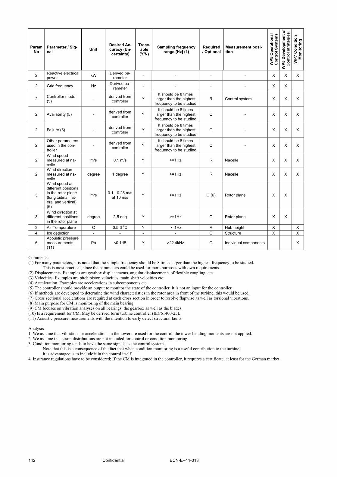
142 Confidential ECN-E--11-013
Param No
Parameter / Sig-nal Unit
Desired Ac-curacy (Un-certainty)
Trace-able (Y/N)
Sampling frequency range [Hz] (1)
Required / Optional
Measurement posi-tion
WP5
Ope
ratio
nal
Con
trol
Sys
tem
s
WP5
Dev
elop
men
t of
Con
trol
str
ateg
ies
WP7
Con
ditio
n M
onito
ring
2 Reactive electrical power kW Derived pa-
rameter - - - - X X X
2 Grid frequency Hz Derived pa-rameter - - - - X X
2 Controller mode (5) - derived from
controller Y It should be 8 times
larger than the highest frequency to be studied
R Control system X X X
2 Availability (5) - derived from controller Y
It should be 8 times larger than the highest frequency to be studied
O - X X X
2 Failure (5) - derived from controller Y
It should be 8 times larger than the highest frequency to be studied
O - X X X
2 Other parameters used in the con-troller
- derived from controller Y
It should be 8 times larger than the highest frequency to be studied
O - X X X
2 Wind speed measured at na-celle
m/s 0.1 m/s Y >=1Hz R Nacelle X X X
2 Wind direction measured at na-celle
degree 1 degree Y >=1Hz R Nacelle X X X
3
Wind speed at different positions in the rotor plane (longitudinal, lat-eral and vertical) (6)
m/s 0.1 - 0.25 m/s at 10 m/s Y >=1Hz O (6) Rotor plane X X
3 Wind direction at different positions in the rotor plane
degree 2-5 deg Y >=1Hz O Rotor plane X X
3 Air Temperature C 0.5-3 oC Y >=1Hz R Hub height X X 4 Ice detection - - - - O Structure X X
6 Acoustic pressure measurements (11)
Pa <0.1dB Y >22.4kHz O Individual components X
Comments: (1) For many parameters, it is noted that the sample frequency should be 8 times larger than the highest frequency to be studied. This is most practical, since the parameters could be used for more purposes with own requirements. (2) Displacements. Examples are gearbox displacements, angular displacements of flexible coupling, etc. (3) Velocities. Examples are pitch piston velocities, main shaft velocities etc. (4) Acceleration. Examples are accelerations in subcomponents etc. (5) The controller should provide an output to monitor the state of the controller. It is not an input for the controller. (6) If methods are developed to determine the wind characteristics in the rotor area in front of the turbine, this would be used. (7) Cross sectional accelerations are required at each cross section in order to resolve flapwise as well as torsional vibrations. (8) Main purpose for CM is monitoring of the main bearing. (9) CM focuses on vibration analyses on all bearings, the gearbox as well as the blades. (10) Is a requirement for CM. May be derived form turbine controller (IEC61400-25). (11) Acoustic pressure measurements with the intention to early detect structural faults. Analysis 1. We assume that vibrations or accelerations in the tower are used for the control, the tower bending moments are not applied. 2. We assume that strain distributions are not included for control or condition monitoring. 3. Condition monitoring tends to have the same signals as the control system. Note that this is a consequence of the fact that when condition monitoring is a useful contribution to the turbine, it is advantageous to include it in the control itself. 4. Insurance regulations have to be considered; If the CM is integrated in the controller, it requires a certificate, at least for the German market.
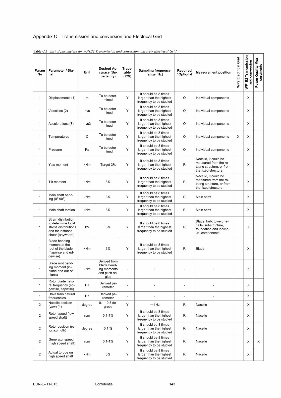
ECN-E--11-013 Confidential 143
Appendix C Transmission and conversion and Electrical Grid
Table C.1 List of parameters for WP1B2 Transmission and conversion and WP9 Electrical Grid
Param No
Parameter / Sig-nal Unit
Desired Ac-curacy (Un-certainty)
Trace-able (Y/N)
Sampling frequency range [Hz]
Required / Optional Measurement position
WP9
Ele
ctric
al G
rid
WP1
B2
Tran
smis
sion
an
d co
nver
sion
Pow
er Q
ualit
y M
ea-
sure
men
ts
1 Displacements (1) m To be deter-mined Y
It should be 8 times larger than the highest frequency to be studied
O Individual components X
1 Velocities (2) m/s To be deter-mined Y
It should be 8 times larger than the highest frequency to be studied
O Individual components X
1 Accelerations (3) m/s2 To be deter-mined Y
It should be 8 times larger than the highest frequency to be studied
O Individual components X
1 Temperatures C To be deter-mined Y
It should be 8 times larger than the highest frequency to be studied
O Individual components X X
1 Pressure Pa To be deter-mined Y
It should be 8 times larger than the highest frequency to be studied
O Individual components X
1 Yaw moment kNm Target 3% Y It should be 8 times
larger than the highest frequency to be studied
R
Nacelle, it could be measured from the ro-tating structure, or from the fixed structure.
X
1 Tilt moment kNm 3% Y It should be 8 times
larger than the highest frequency to be studied
R
Nacelle, it could be measured from the ro-tating structure, or from the fixed structure.
X
1 Main shaft bend-ing (0° 90°) kNm 3% Y
It should be 8 times larger than the highest frequency to be studied
R Main shaft X
1 Main shaft torsion kNm 3% Y It should be 8 times
larger than the highest frequency to be studied
R Main shaft X
1
Strain distribution to determine local stress distributions and for instance shear (anywhere)
kN 3% Y It should be 8 times
larger than the highest frequency to be studied
R
Blade, hub, tower, na-celle, substructure, foundation and individ-ual components
X
1
Blade bending moment at the root of the blade (flapwise and ed-gewise)
kNm 3% Y It should be 8 times
larger than the highest frequency to be studied
R Blade X
1
Blade root bend-ing moment (in-plane and out-of-plane)
kNm
Derived from blade bend-ing moments and pitch an-
gles
- - - - X
1 Rotor blade natu-ral frequency (ed-gewise, flapwise)
Hz Derived pa-rameter - - - - X
1 Drive train natural frequencies Hz Derived pa-
rameter - - - - X
2 Nacelle position (yaw) (4) degree 0.1 - 0.5 de-
grees Y >=1Hz R Nacelle X
2 Rotor speed (low speed shaft) rpm 0.1-1% Y
It should be 8 times larger than the highest frequency to be studied
R Nacelle X
2 Rotor position (ro-tor azimuth) degree 0.1 % Y
It should be 8 times larger than the highest frequency to be studied
R Nacelle X
2 Generator speed (high speed shaft) rpm 0.1-1% Y
It should be 8 times larger than the highest frequency to be studied
R Nacelle X X
2 Actual torque on high speed shaft kNm 3% Y
It should be 8 times larger than the highest frequency to be studied
R Nacelle X
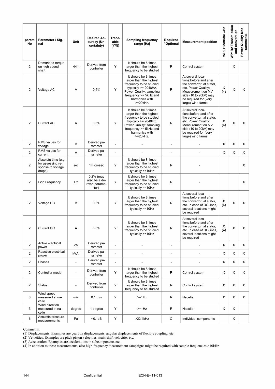
144 Confidential ECN-E--11-013
param No
Parameter / Sig-nal Unit
Desired Ac-curacy (Un-certainty)
Trace-able (Y/N)
Sampling frequency range [Hz]
Required / Optional Measurement position
WP9
Ele
ctric
al G
rid
WP1
B2
Tran
smis
sion
an
d co
nver
sion
Pow
er Q
ualit
y M
ea-
sure
men
ts
2 Demanded torque on high speed shaft
kNm Derived from controller Y
It should be 8 times larger than the highest frequency to be studied
R Control system X
2 Voltage AC V 0.5% Y
It should be 8 times larger than the highest
frequency to be studied, typically >= 2048Hz.
Power Quality: sampling frequency >= 5kHz and
harmonics with >=20kHz.
R
At several loca-tions;before and after the convertor, at stator, etc. Power Quality: Measurement on MV side (10 to 20kV) may be required for (very large) wind farms.
X (4) X X
2 Current AC A 0.5% Y
It should be 8 times larger than the highest
frequency to be studied, typically >= 2048Hz.
Power Quality: sampling frequency >= 5kHz and
harmonics with >=20kHz.
R
At several loca-tions;before and after the convertor, at stator, etc. Power Quality: Measurement on MV side (10 to 20kV) may be required for (very large) wind farms.
X (4) X X
2 RMS values for voltage V Derived pa-
rameter - - - - X X X
2 RMS values for current A Derived pa-
rameter - - - - X X X
2
Absolute time (e.g. for assessing re-sponse to voltage drops)
sec 1microsec Y
It should be 8 times larger than the highest
frequency to be studied, typically >=10Hz
R - X
2 Grid Frequency Hz
0.2% (may also be a de-rived parame-
ter)
Y
It should be 8 times larger than the highest
frequency to be studied, typically >=10Hz
R - X
2 Voltage DC V 0.5% Y
It should be 8 times larger than the highest
frequency to be studied, typically >=10Hz
R
At several loca-tions;before and after the convertor, at stator, etc. In case of DC-lines, several locations might be required
X (4) X X
2 Current DC A 0.5% Y
It should be 8 times larger than the highest
frequency to be studied, typically >=10Hz
R
At several loca-tions;before and after the convertor, at stator, etc. In case of DC-lines, several locations might be required
X (4) X X
2 Active electrical power kW Derived pa-
rameter - - - - X X X
2 Reactive electrical power kVAr Derived pa-
rameter - - - - X X X
2 Phases - Derived pa-rameter - - - - X X X
2 Controller mode - Derived from controller Y
It should be 8 times larger than the highest frequency to be studied
R Control system X X X
2 Status - Derived from controller Y
It should be 8 times larger than the highest frequency to be studied
R Control system X X X
3 Wind speed measured at na-celle
m/s 0.1 m/s Y >=1Hz R Nacelle X X X
3 Wind direction measured at na-celle
degree 1 degree Y >=1Hz R Nacelle X X
6 Acoustic pressure measurements Pa <0.1dB Y >22.4kHz O Individual components X
Comments: (1) Displacements. Examples are gearbox displacements, angular displacements of flexible coupling, etc (2) Velocities. Examples are pitch piston velocities, main shaft velocities etc. (3) Acceleration. Examples are accelerations in subcomponents etc. (4) In addition to these measurements, also high-frequency measurement campaigns might be required with sample frequencies >10kHz

ECN-E--11-013 Confidential 145
Appendix D Flow and Remote Sensing
Table D.1 List of parameters for WP8 Flow and WP6 Remote Sensing
Param No
Parameter / Sig-nal Unit
Desired Ac-curacy (Un-certainty)
Trace-able (Y/N)
Sampling frequency range [Hz]
Required / Optional Measurement position
WP6
Rem
ote
Sens
ing
WP8
Flo
w C
hara
cter
isat
ion
with
in a
nd a
roun
d w
ind
farm
3
Wind speed (longi-tudinal, lateral and vertical) covering the rotor plane, below and above
m/s 0.1m/s Y >=1Hz R
From 10m to one and a half times tip height; at several distances be-fore and behind the tur-bine
X X
3
Wind direction (longitudinal, lat-eral and vertical) covering the rotor plane, below and above
degree 1 degree Y >=1Hz R
From 10m to one and a half times tip height; at several distances be-fore and behind the tur-bine
X X
3
Turbulence in the wind %
derived pa-rameter from
horizontal wind speed
- - O Rotor plane, free sector X X
3 Air Temperature oC 0.5-3 oC Y >=1Hz R Hub height, ground lev-el X X
3
Temperature dif-ference
oC 0.01-0.1 oC Y >=1Hz O
Rotor plane; offshore the difference between air temperature and sea water temperature may be dominating
X X
3 Air relative humidi-ty % 3% Y >=1Hz O Hub height, ground lev-
el X X
3 Atmospheric pres-sure hPa 5 hPa Y >=1Hz R Hub height, ground lev-
el X X
2 WT status signal - derived from
controller Y >=1Hz R Control system X
2 WT Grid Con-nected signal - derived from
controller Y >=1Hz O Control system X
2 Blade condition - icing, dust, insects - - - - O Blades X
2 Rotor speed (low speed shaft) RPM 0.1-1% Y 1-10Hz O - X
2 Pitch angle degree 0.1-0.5 de-gree Y 1-10Hz R - X
2 Control Settings - derived from
controller Y >=1Hz O - X
2 Nacelle position (yaw) degree 0.1-0.5 de-
gree Y >=1Hz R Nacelle X
2 Nacelle anemo-meter m/s 0.1m/s Y >=1Hz R Nacelle X
2 Active electrical power kW 0.5% Y >=1Hz R
Between wind turbine and electrical connec-tion
X
Comments: Remote sensing is performed from the ground, or could be performed from the wind turbine or mast. Remote sensing from the nacelle could be
1. pointed to the front (inflow wind field), 2. pointed to the back (wake), pointed up (flow above wind farm).
Remote sensing from a mast could for instance assist the (complex terrain) power performance analysis.

146 Confidential ECN-E--11-013
Appendix E Power Performance analysis (IEC 61400-12-1)
Table E.1 List of parameters for Power Performance analysis according IEC 61400-12-1.
Param No
Parameter / Signal Unit
Desired Accu-racy (Uncer-
tainty)
Trace-able (Y/N)
Sampling frequency range [Hz]
Required / Optional Measurement position
Pow
er P
erfo
r-m
ance
Site
Cal
ibra
tion
2 Active electrical power kW 0.5% Y >=1Hz R Between wind turbine and
electrical connection X
2 Reactive elec-trical Power kVAr 0.5% Y >=1Hz O Between wind turbine and
electrical connection X
2 WT Availability Status signal - derived from
controller Y >=1Hz R Control system X
2 WT Grid Con-nected signal - derived from
controller Y >=1Hz O Control system X
2 Blade condition - icing, dust, in-sects
(1) - - - O Blades X
2 Rotor speed (low speed shaft)
rpm 0.1-1% Y >=1Hz O - X
2 Pitch angle degree 0.1-0.5 degree Y >=1Hz O - X
2 Control Settings - derived from controller Y >=1Hz O Control system X
2 Nacelle position (yaw) degree 0.1-0.5 degree Y >=1Hz O - X
2 Yaw misalign-ment degree
Derived parame-ter from nacelle
position and wind direction
- - O - X
3 Wind speed, ho-rizontal compo-nent
m/s 0.1 - 0.25 m/s at 10 m/s Y >=1Hz R Hub height, free sector X X
3 Wind speed, ho-rizontal compo-nent
m/s 0.1 - 0.25 m/s at 10 m/s Y >=1Hz R Hub height on a mast at
the turbine location X
3 Wind speed measured at other heights
m/s 0.1-0.25 m/s at 10 m/s Y >=1Hz O Rotor plane, free sector X X
3 Wind speed, vertical compo-nent
m/s 0.1 - 0.25 m/s Y >=1Hz O Rotor plane, free sector X X
3 Turbulence in the wind %
Derived parame-ter from horizon-tal wind speed
- - O Rotor plane, free sector X X
3 Wind direction degree 2-5 deg Y >=1Hz R Rotor plane, free sector X X
3 Air Temperature oC 0.5-3 oC Y >=1Hz Power perfor-mance: R Site calibration: O
Hub height X X
3 Temperature difference
oC 0.01-0.1 oC Y >=1Hz O Rotor plane X X
3 Air relative hu-midity % 3% Y >=1Hz O Hub height X X
3 Atmospheric pressure hPa 5 hPa Y >=1Hz
Power perfor-mance: R Site calibration: O
Hub height X X
3 Atmospheric Stability [-]
Derived from wind speed
measurements in the rotor plane and temperature
difference
- - O - X X

ECN-E--11-013 Confidential 147
Appendix F Noise Measurements (IEC 61400-11)
Table F.1 List of parameters for Noise measurements according IEC 61400-11.
Param No
Parameter / Signal Unit
Desired Accu-racy (Uncer-
tainty)
Trace-able (Y/N)
Sampling frequency range [Hz]
Required / Optional Measurement position
Noi
se M
ea-
sure
men
ts
2 Active electrical power kW 0.5% Y >=1Hz R Between wind turbine and
electrical connection X
2 Rotor speed (low speed shaft)
rpm 0.1-1% Y >=1Hz R - X
2 Pitch angle deg 0.1-0.5 degree Y >=1Hz R - X
2 Control Settings - Derived from controller Y >=1Hz R Control system X
3 Wind speed ho-rizontal m/s 0.1 - 0.25 m/s at
10 m/s Y >=1Hz R Rotor plane, free sector X
3 Wind speed ho-rizontal m/s 0.1 - 0.25 m/s at
10 m/s Y >=1Hz R Nacelle wind speed X
3 Turbulence in the wind %
Derived parame-ter from horizon-tal wind speed
R Rotor plane, free sector X
3 Wind direction deg 2-5 deg Y >=1Hz O Rotor plane, free sector X 3 Air Temperature oC 0.5-3 oC Y >=1Hz R Hub height X
3 Air relative hu-midity % 3% Y >=1Hz O Hub height X
3 Atmospheric pressure hPa 5 hPa Y >=1Hz R Hub height X
3 Atmospheric Stability [-]
Derived from wind speed
measurements in the rotor plane and temperature
difference
O - X
6 Acoustic pres-sure Pa
<0.1dB Y >22.4kHz R
On a ground plate behind the turbine X