urbanization, health and inequality in the developing world van de poel phd.pdf · urbanization,...
TRANSCRIPT

Urbanization, Health and Inequality in the Developing World
Ellen Van de Poel

Copyright cover: © Werner Bischof / Magnum Photos / www.wernerbischof.comLayout and printing: Optima Grafische Communicatie, Rotterdam, The Netherlands

Urbanization, Health and Inequality in the Developing World
Urbanisatie, gezondheid en ongelijkheid in ontwikkelingslanden
Thesis to obtain the degree of Doctor from the Erasmus University Rotterdam
by command of the rector magnificus
Prof.dr. H.G. Schmidt
and in accordance with the decision of the Doctorate Board
The public defense shall be held onThursday the 24th of September 2009 at 15.30 o’clock
by Ellen Van de Poel
born in Geel, Belgium

Doctoral Committee
Promotor: Prof.dr. E.K.A. Van DoorslaerCo-promotor: dr. O.A. O’Donnell
Other members: Prof.dr. M. Grimm Prof.dr. J.P. Mackenbach Prof.dr. M.P. Pradhan

Table of contents
Publications and working papers 7
Chapter 1: Introduction 9
Chapter 2: Socioeconomic inequality in malnutrition in developing countries 19
Chapter 3: Malnutrition and the disproportional burden on the poor: the case of Ghana
33
Chapter 4: Are urban children really healthier? Evidence from 47 developing countries
51
Chapter 5: What explains the rural-urban gap in infant mortality —household or community characteristics?
73
Chapter 6: Urbanization and the spread of diseases of affluence in China 99
Chapter 7: The health penalty of China’s rapid urbanization 131
Chapter 8: Conclusion and policy recommendations 157
References 165
Samenvatting (Summary in Dutch) 177
Curriculum vitae 183
Acknowledgements 185


Publications and working papers
Chapters 2 to 7 are based on the following articles:
Chapter 2Socioeconomic inequality in malnutrition in developing countriesVan de Poel E, Hosseinpoor A, Speybroeck N, Van Ourti T, Vega J. Socioeconomic inequality in malnutrition in developing countries. Bulletin of the World Health Organization 2008, 84(4): 282-291.
Chapter 3Malnutrition and the disproportional burden on the poor: the case of GhanaVan de Poel E, Hosseinpoor A, Jehu-Appiah C, Vega J, Speybroeck N. Malnutrition and the disproportional burden on the poor: The case of Ghana. International Journal for Equity in Health 2007, 6: 21.
Chapter 4Are urban children really healthier? Evidence from 47 developing countriesVan de Poel E, O’Donnell O, van Doorslaer E. Are urban children really healthier? Evidence from 47 developing countries. Social Science and Medicine 2007, 65: 1986-2003.
Chapter 5What explains the rural-urban gap in infant mortality – household or community charac-teristics?Van de Poel E, O’Donnell O, van Doorslaer E. What explains the urban-rural gap in infant mortality – household or community characteristics? Demography, forthcoming.
Chapter 6Urbanization and the spread of diseases of affluence in ChinaVan de Poel E, O’Donnell O, van Doorslaer E. Urbanization and the spread of diseases of affluence in China. Economics and Human Biology 2009, 7: 200-216.
Chapter 7The health penalty of China’s rapid urbanizationVan de Poel E, O’Donnell O, van Doorslaer E. The health penalty of China’s rapid urbanization. Tinbergen Discussion Paper 2009 09-016/3.


1Introduction
10 Chapter 1
Urbanization, development and health
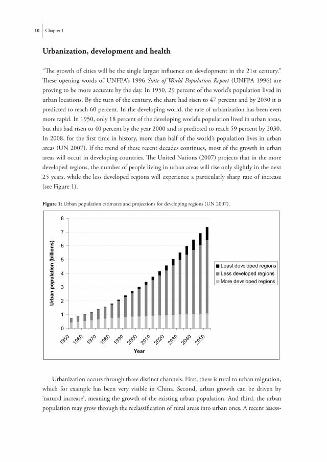
“The growth of cities will be the single largest influence on development in the 21st century.” These opening words of UNFPA’s 1996 State of World Population Report (UNFPA 1996) are proving to be more accurate by the day. In 1950, 29 percent of the world’s population lived in urban locations. By the turn of the century, the share had risen to 47 percent and by 2030 it is predicted to reach 60 percent. In the developing world, the rate of urbanization has been even more rapid. In 1950, only 18 percent of the developing world’s population lived in urban areas, but this had risen to 40 percent by the year 2000 and is predicted to reach 59 percent by 2030. In 2008, for the first time in history, more than half of the world’s population lives in urban areas (UN 2007). If the trend of these recent decades continues, most of the growth in urban areas will occur in developing countries. The United Nations (2007) projects that in the more developed regions, the number of people living in urban areas will rise only slightly in the next 25 years, while the less developed regions will experience a particularly sharp rate of increase (see Figure 1).
Figure 1: Urban population estimates and projections for developing regions (UN 2007). Figure 1: Urban population estimates and projections for developing regions (UN 2007).
0
1
2
3
4
5
6
7
8
1950
1960
1970
1980
1990
2000
2010
2020
2030
2040
2050
Year
Urb
an p
opul
atio
n (b
illio
ns)
Least developed regionsLess developed regionsMore developed regions
Figure 2: Urban slum population estimates and projections for developing regions (UN HABITAT 2001).
0
0.2
0.4
0.6
0.8
1
1.2
1.4
1.6
1990 2001 2005 2010 2015 2020
Year
Urb
an s
lum
pop
ulat
ion
(bill
ions
)
AsiaLatin America and CarribeanSub-Saharan AfricaNorthern AfricaDeveloped regions
Urbanization occurs through three distinct channels. First, there is rural to urban migration, which for example has been very visible in China. Second, urban growth can be driven by ‘natural increase’, meaning the growth of the existing urban population. And third, the urban population may grow through the reclassification of rural areas into urban ones. A recent assess-

Introduction 11
ment of the components of urban growth between 1961 and 2001 found that the share of urban growth attributable to urban natural increase ranged from 51% to about 65% (UNFPA 2007).
To some extent, contemporary development goes hand in hand with urbanization. The urbanization process has played an important positive role in overall global poverty reduction (Ravallion, Chen and Sangraula 2007). National income and level of human development are strongly and positively correlated with the level of urbanization (Bloom & Khanna 2007). However, while the urban population is growing rapidly, so is the problem of urban poverty. Even though urbanization may increase average incomes, at the same time it also increases the number of urban poor and this at a faster rate than the increase in the urban population (Bloom & Khanna 2007). Poor urban populations often resort to urban slums where living conditions are inadequate and employment opportunities limited. UN-HABITAT (2001) estimates that the number of slum dwellers passed 1 billion in 2005, and could reach almost 1.5 billion in 2020, although there are large variations across regions (see Figure 2).
Figure 2: Urban slum population estimates and projections for developing regions (UN HABITAT 2001).
Figure 1: Urban population estimates and projections for developing regions (UN 2007).
0
1
2
3
4
5
6
7
8
1950
1960
1970
1980
1990
2000
2010
2020
2030
2040
2050
Year
Urb
an p
opul
atio
n (b
illio
ns)
Least developed regionsLess developed regionsMore developed regions
Figure 2: Urban slum population estimates and projections for developing regions (UN HABITAT 2001).
0
0.2
0.4
0.6
0.8
1
1.2
1.4
1.6
1990 2001 2005 2010 2015 2020
Year
Urb
an s
lum
pop
ulat
ion
(bill
ions
)
AsiaLatin America and CarribeanSub-Saharan AfricaNorthern AfricaDeveloped regions
What urbanization has in store for the health of populations in the developing world is therefore not clear. Generally, urban populations are found to have better average health than their rural counterparts. But given these large (and increasing) numbers of urban slum dwellers, these averages may mask huge disparities within urban areas. Urban populations can benefit from better access to health services, information and education, and have higher cash incomes and more economic opportunities (Smith et al 2005). But these benefits are often not within reach for the growing urban slum populations who are exposed to living conditions that are

12 Chapter 1
detrimental to health. Further, the pollution problems, increased danger of traffic accidents and social detachment that are prevalent in cities will penalize population health. The rapid environmental, economic and social changes that follow urbanization increase the prevalence of major risk factors for chronic disease, such as obesity and hypertension (Popkin 2001). And rapid -unplanned- urban growth can lead to population demands that outstrip environmental capacity in terms of drinking water, waste disposal and sanitation (Moore et al 2003).
Even though there is much we can say about the immense urbanization process and its health effects in the developing world, there are still many questions to be answered. How large are poor-rich and urban-rural disparities in health? Which are the most important factors driving these inequalities? Are urban populations really better off in terms of health outcomes, or is it just a lucky few that benefit from the urban health advantage? What is happening to these inequalities across time? And, perhaps most importantly, how will the process of urbanization affect population health? This thesis aims at providing answers to these questions and in doing so the intention is to shed light on the complex interlinkages between urbanization, develop-ment and inequalities in population health in the developing world.
The first part of the thesis (Chapter 2 and 3) looks at socioeconomic inequalities in health. Here there is less focus on urbanization and health. Chapters 4 to 6 focus more explicitly on health inequalities across areas at different stages of the urbanization process. Chapter 7 quanti-fies the causal health effects of the urbanization process. Finally, Chapter 8 provides a discussion of the thesis’ main research findings and the way in which these are relevant for development policy purposes. In the remainder of this Introduction we elaborate on the specific research questions asked within each of the chapters.
Figure 3: Gini coefficients of income distributions across the world (UNDP 2008).
Figure 3: Gini coefficients of income distributions across the world (UNDP 2008).
Gini coefficient
0.30-0.340.35-0.390.40-0.440.45-0.490.50-0.540.55-0.59>0.60no data

Introduction 13
Socioeconomic inequalities in health
The average income growth that comes with increasing development and urbanization is not equally divided within (or across) countries. Especially in developing countries, income in-equalities tend to be very large (see Figure 3).
Countries with large income inequalities are likely to have substantial socioeconomic in-equalities in health outcomes as well. While some degree of income inequality may be considered justified, health is considered a universal right to everyone, irrespective of socioeconomic status (WHO 1978). Equity in access to health care is also one of the tenets of the Universal Declara-tion of Human Rights. Therefore, the concept and principles of equity feature in the health policies of most countries and socioeconomic inequalities in health are generally considered undesirable by policy makers.
A first question addressed in this thesis is how large these socioeconomic inequalities in health outcomes are in the developing world. Are they similar across different health indicators? Do some regions have larger inequalities than others? And is there a relationship between aver-age prevalence rates of ill-health conditions and socioeconomic inequalities in ill-health? Given the focus of international development targets, such as the Millenium Development Goals (UN 2006), on average rates of ill-health, it is of interest to establish how countries compare on average rates and inequalities in ill-health outcomes. Chapter 2 provides some answers to these questions by studying socioeconomic inequalities in childhood malnutrition outcomes across a large set of 47 developing countries. Child health outcomes have the advantage of being very sensitive to conditions that affect general population health, being quite easy to collect and available for a very large set of developing countries through the Demographic and Health Surveys (DHS). Socioeconomic inequalities in childhood malnutrition are quantified by means of an adjusted concentration index (Wagstaff et al 1991; Erreygers 2008). This index measures the extent to which malnutrition is concentrated among poor or rich children and has some useful characteristics: (i) negative values imply that malnutrition is more concentrated among poorer children and vice versa, (ii) if all children, irrespective of their socioeconomic status, would equally suffer from malnutrition, the index would equal zero, and (iii) transferring malnutrition from a richer to a poorer individual reduces socioeconomic inequality. In addition to quantifying the degree of socioeconomic inequality by a single index, we also illustrate the different patterns of the distribution of malnutrition across socioeconomic groups. The results in Chapter 2 illustrate that large socioeconomic inequalities in malnutrition are present in the developing world, and that these are not systematically related to average rates of malnutrition.
Clearly, the large socioeconomic inequalities in health outcomes in the developing world are related to the inequalities in the income distribution. However, this does not necessarily mean that to reduce socioeconomic inequality in health, policy makers should only strive to reduce income inequality. Other mechanisms, such as ensuring free access to health care or education might be very efficient in raising the health status of poorer population groups and
14 Chapter 1
therefore reduce socioeconomic inequalities in health. Also targeting policies towards specific areas within a country can be an efficient way to reduce socioeconomic inequalities in health. As discussed before, development and urbanization usually go hand in hand, both across and within countries. Therefore, socioeconomic inequalities in health outcomes might to a large extent reflect urban-rural inequalities in health. If this is indeed the case, it would be efficient to target policy to rural areas as these are usually much easier to identify than poor population groups. The third Chapter of this thesis investigates which factors are mostly responsible for socioeconomic inequalities in childhood malnutrition, hereby providing some indication of which policy initiatives would be most successful in reducing these inequalities. The analysis uses DHS data from Ghana, which is characterized by large socioeconomic and regional in-equalities. In response to the deteriorating child health indicators, the Ghanaian government adopted in 2006 an approach that addressed the broader determinants of health, which has thus generated interest in socio-economic inequalities in health and malnutrition and therefore makes the study very relevant for policy purposes (Ghana Ministry of Health 2006). To explain socioeconomic inequalities in child malnutrition, we use the decomposition framework that was proposed by Wagstaff, van Doorslaer et al (2003). This framework allows decomposing socioeconomic inequalities in childhood malnutrition, in terms of a concentration index, into inequalities in the determinants of malnutrition. For a determinant, say e.g. parents’ educa-tion, to contribute to socioeconomic inequalities in malnutrition, it needs to be sufficiently associated with the malnutrition outcome and unequally distributed across income groups. The results of the analysis in Chapter 3 indicate that socioeconomic inequalities in malnutrition in Ghana are indeed related to many factors, including poverty, health care use and regional inequalities. However, socioeconomic inequalities in malnutrition do not seem to closely follow the urban-rural divide. After controlling for a broad set of household characteristics, we do not find a significant relationship between the urban-rural dichotomy and child malnutrition. Does this mean that urban-rural health disparities are just attributable to different population characteristics at these various locations? In Chapter 4 we shift the focus of the thesis more explicitly to studying the magnitude and causes of urban-rural inequalities in health outcomes across the developing world.
Urban-rural and urbanicity related inequalities in health
There is quite some evidence that urban areas have better average health outcomes than rural ones (see Chapter 4, Table 1). But how large are these urban-rural health inequalities across the developing world? Do they vary across different regions or different health indicators? Can they easily be explained by socio-demographic population characteristics, as suggested by the case study of Ghana in Chapter 3? Chapter 4 provides an answer to these questions by investigating urban-rural inequalities in childhood malnutrition and mortality in the same set of 47 develop-

Introduction 15
ing countries as studied in Chapter 2. After documenting the magnitude of crude urban-rural inequalities, the disparities that remain after controlling for differences in households’ socio-economic status, living conditions and bio-demographic factors are identified. Thereafter, the study takes a closer look at socioeconomic inequalities in health within urban and rural areas. As discussed before, there is a strong relationship between urbanization and economic develop-ment, with higher average incomes in urban areas. However, in developing countries, some urban locations are growing rapidly through the expansion of slum areas. These often pose severe threats to population health in the form of overcrowding, lack of sanitation and clean drinking water, violence and limited access to health services. Is there still an urban advantage in child health outcomes between the poorest population groups in urban and rural locations? Chapter 4 investigates this by studying urban-rural inequalities within the poorest and richest population groups, and by comparing within urban and within rural socioeconomic inequalities.
The results of the analysis indicate that urban-rural differences in childhood malnutri-tion and mortality are very much related to urban-rural differences in socioeconomic status and less to differences in other socio-demographic factors. However in more than a third of the countries studied, the rural-urban disparity is still significant after controlling for a very broad set of all household characteristics. This might suggest that either insufficient control had been made for household characteristics, or that other factors on the community level are also playing an important role. The importance of community characteristics in explaining urban-rural inequalities has not previously been thoroughly investigated, mostly because survey data including both household and community level information are not often easily available in developing countries. The distinction is nonetheless important since it is helps determine the most appropriate level for policy intervention.
Chapter 5 uses DHS data for a set of six sub-Saharan African countries that do contain both household and community level characteristics to investigate the urban-rural gap in infant mortality. To allow for unobserved heterogeneity at both the household and community level, a three-level random intercept probit model is used to model infant mortality (Gibbons & Hedeker 1997). To get an idea of the relative importance of both observed and unobserved household and community level factors in explaining urban-rural inequalities in infant mortal-ity, we extend an Oaxaca-type decomposition (Oaxaca 1973) for non-linear models suggested by Fairlie (2005) to take account of unobserved household and community level heterogeneity. It is important to control for this heterogeneity as there could be many factors common to households or communities affecting infant mortality rates without being explicitly measured in the data, such as e.g. cross-infection rates, customs and traditions and climate and soil fertility. The decomposition reveals that higher infant mortality rates in rural areas mainly derive from the rural disadvantage in household environmental characteristics such as safe source of drink-ing water, electricity and quality of housing materials.

16 Chapter 1
After having studied urban-rural disparities in health in Chapter 4 and 5, it is found that the urban-rural dichotomy is likely to be an oversimplification of reality. Urban areas are not homo-geneous with respect to their degree of urbanization (McDade & Adair 2001). Within urban or rural areas, communities will differ in terms of population densities, density and integration of transportation systems, economic activity, public infrastructure, access to markets etc. When defining the degree of urbanization in terms of such characteristics, there may be urbanized pockets within wider areas categorized as rural or even vice versa. The larger the heterogeneity in population characteristics and in the degree of urbanization within urban and rural areas, the less meaningful is the urban-rural dichotomy, and the greater the need to move to more sensitive measures of communities’ degrees of urbanization. Chapter 6 develops such a measure of urbanicity1 using longitudinal community data from the China Health and Nutrition Survey (CHNS).
China’s urbanization is unprecedented in human history, both in scale and in speed. The proportion of the Chinese population living in urban areas has rapidly increased from 20% in 1980, to 27% in 1990, and 43% in 2005 (National Bureau of Statistics 2006; World Bank 2006). China will complete in just a few decades the urbanization process which took western developed countries hundreds of years. What does this urbanization process mean in terms of health outcomes? While child mortality and malnutrition rates are relatively low, prevalence rates of ‘diseases of affluence’ such as obesity and hypertension are rising remarkably fast in China (Popkin 2001). Urban areas are shifting to diets dominated by more processed foods and a higher fat content, while the acquisition of new technology and transitions away from a mostly agricultural economy are leading to more sedentary occupations (Popkin & Du 2003; Monda, Gordon-Larsen et al 2007).
Increasing urbanization and development is likely to drastically change the geographical dis-tribution of non-communicable diseases. Chapter 6 investigates how obesity and hypertension rates vary across areas at different stages of urbanization, and how and why this distribution is changing over time. In order to target public health interventions appropriately, it is important to establish whether these disease risk factors are spreading to less urban areas, or whether they are merely rising in the most urban ones. The urbanicity index enables identification of communities at various stages of the urbanization process, and allows tracking the changes in communities’ degrees of urbanicity over time. The index is used to rank communities according to their degree of urbanicity and to apply a concentration index type measure to quantify urba-nicity related inequalities in obesity and hypertension. Similar to the concentration indices used in Chapters 2 and 3, this index of urbanicity related inequality measures the extent to which
1 The term ‘‘urbanization’’ is used to describe the process by which communities become increasingly urban and the term ‘‘urbanicity’’ to describe the degree to which a community has the characteristics of an urban environment. Urbanization is a process, whereas urbanicity is a state at any point in time in that process.

Introduction 17
obesity and hypertension are concentrated in more urban or more rural areas. The longitudinal data allow tracking of changes in this inequality over time.
Building on the decomposition framework that is applied in Chapter 3, we develop a methodology that decomposes urbanicity related inequalities in obesity and hypertension into inequalities in the determinants of these conditions. This takes into account that for a determinant, e.g. fat intake, to contribute to urbanicity related inequalities in obesity or hy-pertension, it needs to be significantly associated with these ill-health outcomes and unevenly distributed across areas with various degrees of urbanicity. The results in Chapter 6 reveal that while prevalence rates of obesity and hypertension almost doubled over the period 1991-2004, the risk factors became less concentrated in more urbanized areas. It appears that, as develop-ment and urbanization are spreading within the Eastern and Central provinces of China, so are the diseases of affluence.
The health effects of urbanization
Chapters 2 to 6 of this thesis have focused on measuring and explaining health inequalities across income groups and geographic areas at different stages of the urbanization process. While decomposing these inequalities at different points in time, which is done in Chapter 6, does provide some insight into the associations between health and urbanization, it does not really get at the causal health effects of urbanization. What really happens to individuals’ health when they are exposed to the urbanization process? While average health is better in urban areas, this does not mean that the process of urbanization necessarily causes an improvement in health. The urbanization process clearly brings about positive, as well as negative health effects. Closer proximity to health care facilities, particularly hospitals, is an obvious advantage of living in towns and cities. Especially in China, urban-rural differences in access to health care, and in health insurance cover, have been marked and widening in recent decades (Liu et al 1999). Access to schools and to health education initiatives confer a strong advantage on urban areas in the field of preventive health care. Urban populations can also experience health benefits from the higher incomes and economic opportunities in urban areas. But, as discussed before, there are also many negative health consequences to urbanization, such as environmental and social degradation, expanding slum areas, traffic accidents, overcrowding, inadequate sanitation systems and increasing risk factors for non-communicable diseases.
Chapter 7 of the thesis presents estimates of the causal net health effect of urbanization in China. This net health effects captures both the negative and positive health effects discussed before and gives some insight into the overall impact of urbanization on the health of the Chi-nese. This is done using the same longitudinal CHNS data and the urbanicity index as used in Chapter 6. Communities that move sufficiently across the distribution of the index are defined as becoming urbanized and difference-in-differences (DID) estimators are used to estimate the

18 Chapter 1
treatment effect of this rapid urbanization (Blundell et al 2004; Puhani 2008). The difficulty with estimating a causal health effect of urbanization, is that we do not know the counterfactual, that is what would have happened to the health of individuals should they not have been exposed to the urbanization process. The idea behind DID techniques is to create a counterfactual from other communities that have not experienced urbanization but are similar in other (observable) characteristics. Then, the comparison of health changes (difference-in-differences) between this control group and the people actually having experienced urbanization provides evidence on the causal health effect of urbanization. As the data are from a panel, the estimates can be made robust to unobserved individual time-invariant heterogeneity. A clear distinction is made between differences in the average health status of people living in more urban versus more rural communities, and the actual health effect of increasing urbanization. The main health outcome in Chapter 7 is a measure of self-assessed health (SAH). Respondents are asked to rate their health on an ordinal scale from excellent to poor. As this measure could be affected by reporting bias, in the sense that individuals change their health expectations and therefore their reporting behavior after experiencing urbanization, it is complemented with other more objective -but also more specific- adult health indicators such as mortality, obesity, hypertension, functional limitations, and symptoms of illnesses. The analysis in Chapter 7 indicates that while more urban populations are indeed in better average health, the actual process of urbanization has a net negative health effect. This makes it unclear whether and for how long the urban health advantage in the Chinese population will remain.

2Socioeconomic inequality in malnutrition in developing countries
The objectives of this study are to report socioeconomic inequalities in child-hood malnutrition in the developing world, to provide evidence on the as-sociation between socioeconomic inequality and average malnutrition, and
to draw attention to the different patterns of socioeconomic inequality in malnutrition. Both stunting and wasting were measured using the new WHO child growth standards. Socioeconomic status was estimated through principal component analysis using a set of household assets and living conditions. Socioeconomic inequality was measured in terms of an alternative concentration index that avoids problems with mean dependence. Within almost all countries in this study, stunting and wasting disproportionably af-fected the poor, although socioeconomic inequalities in wasting were much smaller and insignificant in about one third of the countries. When correcting for mean dependence of the concentration index, there appeared no clear association between average stunting and socioeconomic inequality. The latter showed different patterns that were labelled as mass deprivation, queuing and exclusion. Although average levels of malnutrition were higher when using the new WHO reference standards, estimates of socioeconomic in-equality were fairly robust to this change in growth standards. Socioeconomic inequali-ties in childhood malnutrition were present in the entire developing world, and were not evidently related to average rates of malnutrition. Failure to tackle these inequalities is a cause of social injustice and a reduction of these inequalities does not seem to arrive as a windfall profit from reducing the overall rate of malnutrition. Therefore policies should take into account the entire distribution of childhood malnutrition across socio-economic groups.

20 Chapter 2
Introduction
Epidemiological evidence points to a small set of primary causes of child mortality – pneumo-nia, diarrhea, low birth weight, asphyxia and, in some parts of the world, HIV and malaria – as the main killers of children under five years. Malnutrition is the underlying cause of every one out of two such deaths (Murray & Lopez 1997, Bryce et al 2005). The evidence also shows that child deaths and malnutrition are not equally distributed throughout the world. They cluster in Sub-Saharan Africa and South Asia, and in poor communities within these regions (de Onis & Blossner 2003; de Onis et al 2000). Poor-rich disparities in health outcomes are increasingly drawing the attention of researchers and policy makers, hereby fostering a substantial growth in the health-equity related literature (Gwatkin 2000; Wagstaff 2000; Gwatkin 2001; Braveman & Tarimo 2002). Socioeconomic inequality in malnutrition refers to the degree to which child-hood malnutrition rates differ between more and less socially and economically advantaged groups. This is different from pure inequalities which take into account all variation in childhood malnutrition. The available literature that documents socioeconomic inequality in malnutrition is mainly focused on one specific country or region (Larrea & Freire 2002; Zere & McIntyre 2002; Thang et al 2003; Van Doorslaer and Watanabe 2003; Fotso & Kuate-Defo 2005; Hong 2006). On a more global level, Wagstaff & Watanabe (2000) provided evidence on the socioeco-nomic inequalities in malnutrition across 20 developing countries. Other relevant cross-country studies include those of Pradhan et al (2003) and Smith et al (2005), respectively describing total inequalities and inequalities between urban and rural populations. The latter two studies however provide no evidence on socioeconomic inequalities within developing countries.
This paper contributes to the literature in several ways. First, it updates and enlarges the evidence base on average malnutrition and socioeconomic inequalities in malnutrition, using the most recent Demographic Health Survey data from 47 developing countries. The use of such a large number of countries allows getting insight into the regional clustering of poor-rich malnutrition disparities in the developing world and into the association between average levels of malnutrition and socioeconomic inequality. Given the focus in international development targets on average rates of malnutrition, it is of interest to establish how countries compare on average rates of malnutrition and inequalities in malnutrition. In addition to quantifying the degree of socioeconomic inequality by a single index, the different patterns of the distribution of malnutrition across socioeconomic groups are also illustrated.
Second, this paper measures childhood malnutrition using the new growth standards that have been recently released by the WHO (2006). The new standards are based on children from Brazil, Ghana, India, Norway, Oman and the US and adopt a fundamentally prescriptive approach designed to describe how all children should grow rather than merely describing how children grew in a single reference population at a specified time (Garza & de Onis 2004). For example, the new reference population only includes children from study sites where at least

Socioeconomic inequality in malnutritionin developing countries 21
20% of women are willing to follow breastfeeding recommendations. To our knowledge this is the first study presenting estimates of malnutrition in a large set of countries based upon these new standards. To check sensitivity of the results to this change in reference group, the analysis is also done using the older US National Center for Health Statistics (NCHS) reference population (WHO 1995).
Finally, this paper measures socioeconomic inequality in malnutrition by means of the concentration index, which takes into account inequality across the entire socioeconomic dis-tribution. Applied to binary indicators, such as mortality and stunting, the concentration index depends upon the mean of the indicator. This would impede cross country comparisons due to substantial differences in means across locations. To avoid this problem, we use an alternative but related index recently introduced by Erreygers (2008).
Methods
Data
Data was used from all 47 Demographic Health Surveys (DHS) that contain information on the nutritional status of children aged up to five years. The data represents countries from four regions: 26 countries in sub-Saharan Africa, 7 in the Near East, 5 in South-South East Asia and 9 in Latin America and the Caribbean region. Table 1 shows the countries and datasets used.
Analysis
Anthropometric data on the height-for-age and the weight-for-height of children were used to measure chronic and acute malnutrition respectively. Low height-for-age reflects slowing in skeletal growth, and is considered to be a reliable indicator of long-standing malnutrition in childhood. Low weight-for-height on the other hand indicates a deficit in tissue and fat mass and is more sensitive to temporary food shortages and episodes of illness. Low weight-for-age is also used in the literature, but not used here as it does not discriminate well between temporary and more permanent malnutrition (WHO 1986, 1995; Zere & McIntyre 2003). A child was considered stunted/wasted if its height-for-age/weight-for-height was below minus two standard deviations from the median of the reference population (Zere & McIntyre 2003; Pradhan et al 2003) We used these crude binary indicators of stunting/wasting as their averages are much easier to intuitively interpret – compared to the continuous height-for-age/weight-for-age z-scores – and therefore facilitate the comparison of stunting/wasting rates across socioeconomic groups and across countries.

22 Chapter 2
This paper used the new WHO child growth standards that were released by the World Health Organization in April 2006 (WHO 2006). Robustness of the results against this change from the NCHS growth standards (WHO 1995) was also checked. An indicator of socioeco-nomic status was developed using principal component analysis (Filmer & Pritchett 2001). The indicator combined information on a set of household assets and living conditions: the ownership of a car, phone, TV, radio, fridge, bike and motorcycle; the availability of electricity,
Table 1: Description of DHS datasets.
country country
codeyear of survey
sample size
country country
codeyear of survey
Sample size
Sub-Saharan Africa (SSA) Near East (NE)
Benin BJ 2001 3842 Armenia AM 2000 1517
Burkina Faso BF 2003 8142 Egypt EG 2000 10296
Cameroon CM 2004 3168 Morocco MA 2003/04 5356
Central African Rep* CF 1994/95 2297 Turkey TR 1998 2782
Chad TD 2004 4414 Kazakhstan KZ 1999 566
Comoros* KM 1996 921 Kyrgyzstan Rep* KG 1997 971
Cote d’Ivoire CI 1998/99 1477 Uzbekistan UZ 1996 954
Ethiopia ET 2000 2833 South & Southeast Asia (SSEA)
Gabon GA 2000 3482 Bangladesh BD 2004 5911
Ghana GH 2003 3094 Cambodia KH 2000 3522
Guinea GN 1999 2961 India* IN 1998/99 24989
Kenya KE 2003 4719 Nepal NP 2001 6163
Madagascar MG 2003/04 2908 Pakistan PK 1990/91 4079
Malawi MW 2000 9162 Latin America & Caribbean (LAC)
Mali ML 2001 9382 Bolivia BO 2003 9134
Mauritania MR 2000/01 3306 Brazil BR 1996 4056
Mozambique MZ 2003 3808 Colombia CO 2005 12393
Namibia NA 2000 2925 Dominican Rep DO 2002 9288
Niger* NE 1998 3914 Guatemala GT 1998/99 3879
Nigeria NG 2003 4293 Haiti HT 2000 5510
Rwanda RW 2000 6038 Nicaragua NI 2001 5875
Tanzania TZ 2004 7132 Paraguay PY 1990 3614
Togo* TG 1998 3443 Peru PE 2000 11585
Uganda UG 2000/01 5145
Zambia ZM 2001/02 1932
Zimbabwe ZW 1999 2632
Note: Data marked with * corresponds to births in three years preceding survey instead of five

Socioeconomic inequality in malnutritionin developing countries 23
clean water and a toilet; and the material used to construct the wall, roof and floor of the household dwelling. Socioeconomic inequality in stunting and wasting was calculated by means of a recently proposed generalisation – introduced by Erreygers (2008) (see also Van de Poel et al (2007) for an application) – of the traditional concentration index (C) which was proposed by Wagstaff et al (1991). The generalisation preserves the main characteristics of the traditional concentration index – (i) negative values imply that malnutrition is more concentrated among poorer children and vice versa, (ii) if all children, irrespective of their socioeconomic status, would equally suffer from malnutrition, the C would equal zero, and (iii) transferring malnutri-tion from a richer to a poorer individual reduces socioeconomic inequality – but overcomes several of its methodological shortcomings. In particular for this paper, it is worth mentioning that the generalisation avoids dependence upon the mean of the binary indicator (Wagstaff (2005) discussed a related issue for the bounds of the concentration index). Not correcting for mean dependence would impede cross country comparisons due to substantial differences in means across locations. In addition it would predetermine the association between average levels of malnutrition and socioeconomic inequality.
Since DHS rely on multi-stage sampling procedures, all estimates take account of sampling weights and statistical inference is adjusted for clustering on the level of the primary sampling unit. The statistical inference for the index recently proposed by Erreygers was based on an adapted ver-sion of the convenient regression approach (Wagstaff & Van Doorslaer 2000; O’Donnell et al 2008).
Results
Table 2 shows the socioeconomic inequalities in stunting. In almost all countries, stunting was disproportionably affecting the poor. Concentration indices (based upon the WHO child growth standards and calculated as suggested by Erreygers (2008)) were significant in all coun-tries, except in Madagascar, and ranged from -0.0005 in Madagascar to -0.42 in Guatemala. Socioeconomic inequality in stunting appeared largest in the Latin American and Caribbean (LAC) region, where the median C equaled -0.22.
The results with respect to wasting are presented in Table 3. Wasting was generally more concentrated among the poor, but the socioeconomic inequality was much smaller as compared to stunting. For about one third of the countries socioeconomic inequalities were insignificant. The median concentration index (calculated as suggested by Erreygers (2008)) was largest in South Southeast Asia (SSEA) (-0.05 based upon WHO child growth standards).
Table 2 and Table 3 also show average stunting and wasting rates based upon the new WHO child growth standards and the NCHS growth standards. For both malnutrition indicators, average rates were higher using the new WHO reference standards. However, socioeconomic inequalities were fairly similar across the different growth standards; therefore the following discussion is mainly based upon the WHO child growth standards.

24 Chapter 2
Table 2: Estimated stunting rates in under-five children by quintiles of socioeconomic status, average stunting rates and concentration indices (C) based upon WHO and NCHS growth standards.
CountryPrevalence of stunting by wealth quintiles
based upon MGRSAverage stunting
Average stunting
C C
Q1 Q2 Q3 Q4 Q5 MGRS NCHS MGRS NCHS
Benin 43.78 45.38 39.98 34.96 27.35 38.61 30.37 -0.15 -0.13
Burkina Faso 48.44 46.96 46.49 40.20 27.45 42.98 38.56 -0.15 -0.15
Cameroon 44.19 43.42 38.85 31.25 19.20 36.49 31.68 -0.21 -0.21
CAR 47.26 41.80 39.89 42.03 33.22 39.84 33.65 -0.11 -0.12
Chad 48.62 44.84 46.07 39.43 33.92 44.16 40.95 -0.09 -0.09
Comoros 46.11 47.08 41.45 37.97 26.47 40.53 33.77 -0.15 -0.19
Cote d’Ivoire 38.66 29.41 31.07 26.10 19.28 31.26 25.17 -0.17 -0.17
Ethiopia 60.94 55.04 58.23 54.07 42.27 56.91 51.22 -0.09 -0.10
Gabon 43.46 35.53 26.44 18.17 18.17 26.03 20.65 -0.22 -0.20
Ghana 45.11 38.27 40.42 30.42 20.01 35.62 29.43 -0.19 -0.19
Guinea 39.08 38.87 35.50 32.42 24.95 34.44 26.07 -0.13 -0.11
Kenya 43.18 39.34 35.48 27.98 22.87 35.90 30.56 -0.17 -0.16
Madagascar 53.90 54.72 59.96 58.15 50.51 56.06 48.34 0.00 -0.01
Malawi 60.64 59.59 52.80 57.79 39.32 54.08 49.02 -0.14 -0.14
Mali 48.79 49.60 45.10 42.40 28.43 41.78 37.57 -0.17 -0.17
Mauritania 45.05 41.47 40.69 32.80 31.65 39.25 34.50 -0.14 -0.16
Mozambique 55.79 53.08 53.84 43.45 34.70 51.50 46.16 -0.11 -0.14
Namibia 33.10 31.68 23.87 18.45 25.00 28.07 22.64 -0.13 -0.09
Niger 50.81 49.09 46.26 49.30 36.53 47.05 41.08 -0.08 -0.09
Nigeria 54.30 50.13 49.55 36.33 25.20 43.19 38.41 -0.25 -0.25
Rwanda 52.34 51.60 51.52 47.00 31.88 47.21 42.37 -0.14 -0.15
Tanzania 48.17 48.22 46.44 44.22 23.91 43.63 37.05 -0.15 -0.16
Togo 37.45 34.25 30.05 25.88 19.03 30.37 21.72 -0.16 -0.14
Uganda 45.84 46.75 49.46 42.79 29.00 44.50 38.61 -0.07 -0.08
Zambia 59.53 58.41 58.33 49.88 40.59 53.21 46.15 -0.17 -0.18
Zimbabwe 37.37 34.65 32.33 29.87 23.45 31.48 26.45 -0.11 -0.12
median 46.69 46.06 43.28 38.70 27.40 41.15 35.77 -0.14 -0.15
Bangladesh 58.19 55.89 53.32 43.03 30.26 49.85 43.02 -0.20 -0.20
Cambodia 54.32 52.78 48.60 43.51 39.86 48.47 44.29 -0.15 -0.16
India 56.43 53.35 49.02 45.54 41.56 49.68 43.75 -0.13 -0.13
Nepal 63.76 63.40 58.92 47.08 42.01 56.46 50.51 -0.19 -0.18
Pakistan 61.91 62.94 53.58 49.13 35.98 54.12 49.59 -0.20 -0.24
median 58.19 55.89 53.32 45.54 39.86 49.85 44.29 -0.19 -0.16

Socioeconomic inequality in malnutritionin developing countries 25
Figure 1 plots the average level of stunting against socioeconomic inequality in stunting. For illustrative purposes, the negative of the concentration index (calculated as suggested by Erreygers (2008)) is shown in these figures such that higher values on the y-axes indicate higher socioeconomic inequality in favour of the rich. There was no clear association between average stunting and socioeconomic inequality in stunting (Spearman coefficient=0.20, p-value=0.17). If attention was restricted to socioeconomic inequalities in the LAC region, higher average stunt-ing levels were associated with higher socioeconomic inequalities in stunting. Figure 2 shows the same association for wasting and clearly illustrates the much smaller socioeconomic inequalities in wasting as compared to stunting. There appeared a negative association between average wast-ing and the concentration index of wasting (Spearman coefficient=-0.60, p-value<0.001), mean-ing that countries with higher average wasting tended to have higher socioeconomic inequalities. However, Figure 2 shows that the magnitude of the association was low at best. The low values of the socioeconomic inequalities, combined with the finding that the relative variability in average wasting levels across countries (coefficient of variation=0.68) was higher than that in average
CountryPrevalence of stunting by wealth quintiles
based upon MGRSAverage stunting
Average stunting
C C
Q1 Q2 Q3 Q4 Q5 MGRS NCHS MGRS NCHS
Armenia 25.08 26.01 14.88 14.01 12.45 18.36 13.00 -0.12 -0.09
Egypt 31.80 26.41 22.69 19.23 15.18 24.00 18.66 -0.13 -0.12
Kazakhstan 17.81 14.91 9.29 9.40 6.32 13.93 9.75 -0.10 -0.10
Kyrgyzstan 41.40 37.66 24.36 28.64 18.88 32.89 24.84 -0.18 -0.17
Morocco 34.87 26.06 20.07 16.68 16.02 23.28 18.18 -0.18 -0.17
Turkey 34.25 23.52 17.48 9.50 5.01 19.04 16.01 -0.24 -0.22
Uzbekistan 41.12 38.35 32.21 33.77 36.00 37.46 31.28 -0.07 -0.09
median 34.25 26.06 20.07 16.68 15.18 23.28 18.18 -0.13 -0.13
Bolivia 48.50 39.71 29.68 22.87 14.29 32.43 26.38 -0.31 -0.29
Brazil 29.46 13.25 7.61 5.41 5.42 13.42 10.46 -0.22 -0.19
Colombia 25.14 17.19 13.89 10.59 6.39 15.70 11.52 -0.15 -0.13
Dominican 21.11 13.51 12.44 8.28 7.45 11.76 8.85 -0.12 -0.10
Guatemala 68.45 67.75 64.23 43.06 25.46 52.80 46.37 -0.42 -0.42
Haiti 38.01 33.83 29.97 21.65 11.74 27.10 21.93 -0.22 -0.19
Nicaragua 42.16 31.73 22.14 12.05 9.46 24.67 20.13 -0.30 -0.27
Paraguay 28.52 24.60 20.84 11.00 7.17 18.20 13.92 -0.20 -0.18
Peru 54.91 43.00 24.91 17.00 14.36 31.29 25.42 -0.41 -0.38
median 38.01 31.73 22.14 12.05 9.46 24.67 20.13 -0.22 -0.23
Note: Underscored averages and C indicate insignificance at the 10% level. Concentration indices are calculated as suggested by Erreygers (2008).

26 Chapter 2
stunting levels (coefficient of variation=0.35), suggest that one should not focus too much on the significance of the association between average wasting and socioeconomic inequality in wasting.
When using the traditional concentration index (or the one suggested by Wagstaff (2005)), different results for the association were found, i.e. there appeared a strong positive association
Table 3: Estimated wasting rates in under-five children by quintiles of socioeconomic status, average wasting rates, and concentration indices (C) based upon WHO and NCHS growth standards.
Country Prevalence of wasting by wealth quintiles (%)Average wasting
Average wasting
Odds-ratio
Q1 Q2 Q3 Q4 Q5 MGRS NCHS
SSA
Benin 12.09 12.06 8.42 7.94 5.76 9.33 7.55 2.25
Burkina Faso 22.01 23.04 23.22 21.27 15.50 21.48 18.72 1.54
Cameroon 8.24 8.46 5.86 4.00 2.93 6.23 5.28 2.98
CAR 10.64 10.79 10.53 8.55 7.44 9.25 7.18 1.48
Chad 17.69 14.89 15.90 16.77 15.88 16.09 13.53 1.14
Comoros 15.52 13.78 10.36 5.91 8.43 11.00 8.40 1.99
Cote d’Ivoire 7.80 8.25 5.66 5.06 4.25 6.85 7.80 1.91
Ethiopia 13.11 13.51 13.52 12.19 7.10 12.70 10.71 1.97
Gabon 4.35 3.02 5.33 5.17 3.27 4.26 2.83 1.34
Ghana 8.57 7.90 8.67 10.20 8.15 8.70 7.12 1.06
Guinea 12.38 10.02 10.48 8.34 8.27 9.92 9.17 1.57
Kenya 8.70 5.35 4.80 3.65 7.59 6.23 5.62 1.16
Madagascar 11.83 11.40 9.17 8.95 7.19 10.04 7.75 1.73
Malawi 8.71 7.32 6.92 6.62 5.76 7.02 5.52 1.56
Mali 12.68 15.49 14.24 13.26 9.49 12.91 10.65 1.39
Mauritania 18.25 16.26 15.20 12.04 12.38 15.27 13.40 1.58
Mozambique 8.44 5.88 5.99 5.39 4.70 6.55 4.60 1.87
Namibia 13.76 8.61 7.71 6.53 9.14 9.85 8.91 1.59
Niger 30.78 27.24 27.02 25.25 14.98 25.66 20.63 2.52
Nigeria 12.41 13.76 9.98 10.98 9.11 11.34 9.48 1.41
Rwanda 9.11 10.52 8.69 8.14 7.66 8.88 6.85 1.21
Tanzania 4.62 4.00 3.50 2.93 3.09 3.68 3.12 1.52
Togo 13.86 19.59 13.48 12.17 8.57 13.98 12.42 1.72
Uganda 5.37 5.15 5.99 4.60 3.50 5.11 4.04 1.56
Zambia 5.83 4.70 7.79 5.84 6.39 6.11 4.88 0.91
Zimbabwe 9.87 12.26 9.72 6.38 4.99 8.64 6.44 2.08
median 11.24 10.66 8.93 8.04 7.51 9.29 7.65 1.57

Socioeconomic inequality in malnutritionin developing countries 27
between average stunting and socioeconomic inequality in stunting (Spearman coefficient=0.78, p-value<0.001), whereas the association between average wasting and socioeconomic inequality in wasting was insignificant (Spearman coefficient=0.14, p-value=0.35). This confirms the importance of correction for mean dependence.
Table 2 and Table 3 also show the distribution of stunting and wasting across quintiles of socioeconomic status. These distributions can take different patterns, which are illustrated for three selected countries in Figure 3 (WHO 2003). In Rwanda, socioeconomic inequality in stunting could be characterized as mass deprivation – stunting is highly prevalent within the
Country Prevalence of wasting by wealth quintiles (%)Average wasting
Average wasting
Odds-ratio
Q1 Q2 Q3 Q4 Q5 MGRS NCHS
SSEA
Bangladesh 16.51 16.48 14.62 12.84 11.51 14.72 12.90 1.52
Cambodia 17.33 17.49 13.68 17.93 18.37 16.89 15.01 0.93
India 22.88 21.82 19.22 16.96 17.13 19.82 15.61 1.44
Nepal 12.26 14.51 11.91 9.36 7.53 11.46 9.69 1.72
Pakistan 18.97 12.47 9.16 12.03 7.88 12.56 9.21 2.74
median 17.33 16.48 13.68 12.84 11.51 14.72 12.90 1.52
NE
Armenia 2.19 2.76 2.32 3.27 2.03 2.53 1.97 1.08
Egypt 3.33 3.41 3.20 2.89 2.82 3.17 2.52 1.19
Kazakhstan 3.04 3.09 1.69 0.86 1.76 2.51 1.82 1.75
Kyrgyzstan 3.21 3.43 4.11 3.16 1.06 3.28 3.44 3.09
Morocco 14.22 9.34 9.87 9.19 10.52 10.74 9.31 1.41
Turkey 4.00 3.73 2.27 1.98 2.67 3.01 1.90 1.52
Uzbekistan 19.44 7.41 12.10 13.53 10.26 13.74 11.63 2.11
median 3.33 3.43 3.20 3.16 2.67 3.17 2.52 1.52
LAC
Bolivia 1.77 1.40 2.01 1.79 1.55 1.70 1.24 1.14
Brazil 4.41 2.48 2.24 1.41 2.64 2.75 2.34 1.70
Colombia 1.74 1.69 1.68 1.27 1.12 1.54 1.29 1.56
Dominican 3.16 1.90 2.77 1.88 1.44 2.15 1.70 2.23
Guatemala 2.76 3.86 4.21 1.10 2.71 2.91 2.52 1.02
Haiti 8.09 5.40 5.91 4.05 5.52 5.81 4.61 1.51
Nicaragua 3.86 2.23 2.78 0.87 1.66 2.37 2.07 2.37
Paraguay 0.73 0.56 0.47 0.67 0.39 0.56 0.33 1.89
Peru 2.16 1.02 1.03 0.72 0.71 1.15 0.94 3.09
median 2.96 2.07 2.51 1.34 1.61 2.26 1.88 1.63
Note: Underscored averages and C indicate insignificance at the 10% level. Concentration indices are calculated as suggested by Erreygers (2008).

28 Chapter 2
majority of the population while a small privileged class is much better off. A second pattern, as was seen in Ghana, could be described as queuing – average stunting is lower than in the previous pattern, but richer population groups are better off while the poor had to wait for a
Figure 1: Average stunting versus (-) concentration index.
BJ BF
CM
CFTD
KMCI
ET
GA
GH
GNKE
MG
MW
ML
MRMZ
NA
NE
NG
RWTZ
TG
UG
ZM
ZW
BD
KH
IN
NPPK
AM EG
KZ
KGMA
TR
UZ
BO
BR
CO
DO
GT
HT
NI
PY
PE
0.0
0.1
0.2
0.3
0.4
0.5
0 10 20 30 40 50 60
Average stunting (%)
(-) C
of s
tunt
ing
SSA SSEA EM LAC median C median stunting
Figure 1: Average stunting versus (-) concentration index. Stunting rates based upon WHO growth standards. Concentration indices are calculated as suggested by Erreygers (2008).
0.0
0.1
0.2
0.3
0.4
0.5
0 10 20 30 40 50 60
Average wasting (%)
(-) C
of w
astin
g
SSA SSEA EM LAC median C median wasting
Figure 2: Average wasting versus (-) concentration index. Stunting rates based upon WHO growth standards. Concentration indices are calculated as suggested by Erreygers (2008).
Note: Stunting rates based upon WHO growth standards. Concentration indices are calculated as suggested by Erreygers (2008).
Figure 2: Average wasting versus (-) concentration index.
BJ BF
CM
CFTD
KMCI
ET
GA
GH
GNKE
MG
MW
ML
MRMZ
NA
NE
NG
RWTZ
TG
UG
ZM
ZW
BD
KH
IN
NPPK
AM EG
KZ
KGMA
TR
UZ
BO
BR
CO
DO
GT
HT
NI
PY
PE
0.0
0.1
0.2
0.3
0.4
0.5
0 10 20 30 40 50 60
Average stunting (%)
(-) C
of s
tunt
ing
SSA SSEA EM LAC median C median stunting
Figure 1: Average stunting versus (-) concentration index. Stunting rates based upon WHO growth standards. Concentration indices are calculated as suggested by Erreygers (2008).
0.0
0.1
0.2
0.3
0.4
0.5
0 10 20 30 40 50 60
Average wasting (%)
(-) C
of w
astin
g
SSA SSEA EM LAC median C median wasting
Figure 2: Average wasting versus (-) concentration index. Stunting rates based upon WHO growth standards. Concentration indices are calculated as suggested by Erreygers (2008). Note: Wasting rates based upon WHO growth standards. Concentration indices are calculated as suggested by Erreygers (2008).

Socioeconomic inequality in malnutritionin developing countries 29
“trickle-down” effect. Third, socioeconomic inequality in stunting in Brazil was in the form of exclusion whereby stunting prevalence is relatively low within the majority of the population, but where a poor minority of the population was deprived.
Discussion
This study illustrates the existence of socioeconomic inequality in malnutrition across the devel-oping world. The results show that malnutrition favours the better-off and that this inequality is much more pronounced for stunting than for wasting. This could be expected as previous evidence has suggested that socioeconomic status has a smaller effect on the stochastic condi-tions that precipitate wasting (e.g. unforeseen environmental factors and diseases) than it has on long-term malnourishment (Wagstaff & Watanabe 2000; Zere & McIntyre 2003). Socioeco-nomic inequalities in stunting were largest in the Latin American and Caribbean region, with Guatemala being an outlier, which is also in line with previous findings (Wagstaff & Watanabe 2000; Larrea & Freire 2002; Larrea et al 2005) .
Average wasting and stunting rates based upon the WHO child growth standards were larger than those based upon the NCHS reference population. This has also been found by de Onis et al (2006) for Bangladesh, Dominican Republic and a pooled sample of North American and European children. However, estimates of socioeconomic inequalities in both stunting and wasting were similar across the different growth standards, as were the associations between socioeconomic inequalities and averages.
Figure 3: Distribution of stunting across quintiles of socioeconomic status for three selected countries.
0
10
20
30
40
50
60
Q1 Q2 Q3 Q4 Q5
% o
f chi
ldre
n stu
nted
Rwanda Ghana Brazil
Figure 3: Distribution of stunting across quintiles of socioeconomic status for three selected countries. Stunting rates based upon WHO growth standards.Note: Stunting rates based upon WHO growth standards.

30 Chapter 2
When studying the association between average malnutrition and socioeconomic inequality in malnutrition, the choice of the inequality index does matter. Using Erreygers’ index (2008), there appeared no clear association between average stunting and socioeconomic inequality in stunting (and some evidence of a limited association for wasting was presented), while the traditional concentration index (or the one suggested by Wagstaff (2005)) gave rather opposite findings. It is worth noting that Wagstaff & Watanabe (2000) found evidence of an inverse relationship between underweight and socioeconomic inequality using the traditional concen-tration index. Applying Erreygers’ index to the data in their paper reversed this finding, which illustrates Erreygers’ point about the need to be careful when comparing concentration indices across countries with highly differing stunting levels.
Socioeconomic inequality was found in different patterns that varied between mass depri-vation, queuing and exclusion. The manner in which systems based on primary health care develop will vary across these differing contexts. In the case of exclusion, programs targeted at specific population groups, i.e. the poorest, are urgently needed to achieve pro-equity outcomes while in other instances, such as mass deprivation, broad strengthening of the whole system or a combination of the two approaches is required (WHO 2003). In this respect, the distribution of malnutrition across socioeconomic groups, as shown in Table 2 and Table 3, can provide a useful tool for health policy makers as it can easily be used to classify countries according to the above mentioned patterns.
There are some limitations to this study. First, it has to be noted that for 6 out of the 47 countries (Central African Republic, Comoros, Niger, Togo, Kyrgyzstan Republic and India) data was only available for children aged 0-3 years instead of 0-5. Since anthropometric deficits accumulate over time, the average malnutrition rates for these countries are underestimated as compared to the other countries. However, as already discussed by Wagstaff & Watanabe (2000), changes in the age limit do not systematically produce an upward or downward bias in socioeconomic inequality. Furthermore, the results were found to be robust to the exclusion of these countries.
Second, the use of an asset index to capture socioeconomic status has its shortcomings. Houweling et al (2003) have shown that the choice of the assets can influence the observed magnitude of health inequalities, but also conclude that in the absence of reliable information on income or expenditure, the use of such an asset index is generally a good alternative to distinguish socioeconomic layers within a population (see also Wagstaff & Watanabe (2003)).
With respect to this study, it is important to note that a separate asset index is constructed for each country. Therefore it is allowed that the correlation between assets and socioeconomic status varies across countries.
Third, this study only investigates socioeconomic inequalities in childhood malnutrition across the developing world and the extent to which these relate to average malnutrition rates. Clearly, this is only a first step in a broader research agenda that analyzes the determinants of socioeconomic inequalities in childhood malnutrition within and across developing countries.

Socioeconomic inequality in malnutritionin developing countries 31
The next step should consist of combining the literature on both socioeconomic and proximate determinants of malnutrition, such as feeding practices, health care seeking behavior and mother’s nutritional status (see e.g. Mosley & Chen 1984; Ruel, Levin et al 1999; Smith et al 2005) with decomposition approaches such as the one proposed by Wagstaff, van Doorslaer et al 2003).
Conclusion
The findings of this study are relevant from both a methodological and policy point of view. Regarding the methodological contribution, this paper is the first to study socioeconomic inequalities in childhood malnutrition in the developing world using the recently introduced WHO child growth standards. It is found that although average malnutrition is higher when us-ing this reference population, estimates of socioeconomic inequality are fairly similar compared to the ones based upon the NCHS reference population. Second, the analysis demonstrates that when studying the association between average malnutrition and the concentration index, it is important to account for mean dependence of the latter index. When doing so, no clear relationship was found between average malnutrition and socioeconomic inequality.
The lack of any relationship between average malnutrition and socioeconomic inequality is also important from a health policy perspective. It suggests that countries with lower average malnutrition levels did not perform fundamentally different in terms of socioeconomic inequali-ties compared to countries with much higher average malnutrition levels. While it is not clear from this study whether this is due to a deliberate policy focus on average malnutrition levels, it shows policy makers should realize that there do not seem to be obvious windfall profits result-ing from focussing on a reduction of average malnutrition levels. Nevertheless, the main goals and targets of large scale development programs such as the Millennium Development Goals continue to be couched in terms of improving population averages (United Nations 2008).
The results of this study also indicate that not only the degree, but also the pattern of socioeconomic inequalities in malnutrition should be a concern in setting health policies. To reduce malnutrition in e.g. many Latin American countries, policies should be targeted to the poor. In contrast, in a lot of Sub-Saharan African countries, next to targeting the poor, there also is a great scope for progress by simply focussing on the general population.


3Malnutrition and the disproportional burden on the poor: the case of Ghana
Malnutrition is a major public health and development concern in the devel-oping world and in poor communities within these regions. Understanding the nature and determinants of socioeconomic inequality in malnutrition
is essential in contemplating the health of populations in developing countries and in targeting resources appropriately to raise the health of the poor and most vulnerable groups. This paper uses a concentration index to summarize inequality in children’s height-for-age z-scores in Ghana across the entire socioeconomic distribution and decomposes this inequality into different contributing factors. Data is used from the Ghana 2003 Demographic and Health Survey. The results show that malnutrition is related to poverty, maternal education, health care and family planning and regional characteristics. Socioeconomic inequality in malnutrition is mainly associated with poverty, health care use and regional disparities. Although average malnutrition is higher using the new growth standards recently released by the World Health Organization, socioeconomic inequality and the associated factors are robust to the change of reference population. Child malnutrition in Ghana is a multisectoral problem. The factors associ-ated with average malnutrition rates are not necessarily the same as those associated with socioeconomic inequality in malnutrition.
34 Chapter 3
Background
In the developing world, an estimated 230 million (39%) children under the age of five are chronically malnourished and about 54% of deaths among children younger than 5 are associ-ated with malnutrition (UNICEF 2000). Malnutrition is a major public health and develop-ment concern with important health and socioeconomic consequences. In Sub-Saharan Africa, the prevalence of malnutrition among the group of under-fives is estimated at 41% (UNICEF 2000). It is the only region in the world where the number of child deaths is increasing and in which food insecurity and absolute poverty are expected to increase (Smith et al 2000; Smith & Haddad 2000). Malnutrition in early childhood is associated with significant functional impairment in adult life, reduced work capacity and decreasing economic productivity (Vella et al 1992; Pelletier et al 1993; Schroeder & Brown 1994; Pelletier & Frongillo 1995; Mendez & Adair 1999; Delpeuch et al 2000). Children who are malnourished not only tend to have increased morbidity and mortality but are also more prone to suffer from delayed mental devel-opment, poor school performance and reduced intellectual achievement (Pelletier et al 1993; Schroeder & Brown 1994; Pelletier & Frongillo 1995).
Chronic malnutrition is usually measured in terms of growth retardation. It is widely ac-cepted that children across the world have much the same growth potential, at least to seven years of age. Environmental factors, diseases, inadequate diet, and the handicaps of poverty appear to be far more important than genetic predisposition in producing deviations from the reference. These conditions, in turn, are closely linked to overall standards of living and the ability of populations to meet their basic needs. Therefore, the assessment of growth not only serves as one of the best global indicators of children’s nutritional status, but also provides an indirect measurement of the quality of life of an entire population (Martorell et al 1992; Lavy et al 1996; de Onis et al 2000).
Large scale development programs such as the Millennium Development Goals (MDGs) have also emphasized the importance of the under-fives’ nutritional status as indicators for eval-uating progress (UN 2006). When aiming at reducing childhood malnutrition, it is important not only to consider averages, which can obscure large inequalities across socioeconomic groups. Failure to tackle these inequalities may act as a brake on making progress towards achieving the MDGs and is a cause of social injustice (UNDP 2005; Nolen et al 2005).
Ghana
Against this background, Ghana provides an interesting case study. The country experienced remarkable gains in health from the immediate post independence era. Life expectancy im-proved over the years and the prevention of a range of communicable diseases improved child survival and development. However in the last decade despite increasing investments in health,
Malnutrition and the disproportional burden on the poor: the case of Ghana 35
Ghana has not achieved target health outcomes. There has been no significant change in Ghana’s under-five and infant mortality rates between 1993 and 2003. In the last couple of years, under-five mortality was actually slightly increasing. Life expectancy has also fallen from 57 years in 2000 to 56 years in 2005 (GSS 2003). Ghana’s Human Development Index (HDI), a measure combing life expectancy, literacy, education and standard of living, has been worsening too; after improving from 0.444 in 1975 to 0.563 in 2001, the HDI dropped to 0.520 in 2005 (UNDP 2005). Since 1988, there has been no definite trend in malnutrition (in terms of height-for-age). Apparent gains between 1988 and 1998 were reversed in 2003 (ORC Macro 2005). Although the 2003 Ghana Demographic Health Survey (DHS) final report (GSS 2003) recommends caution when using data from the various DHS to assess the trend in the nutritional status, it is noted that there was a trend over the past five years of increased stunting compared to a decrease of wasting and underweight. Further, there has been a trend of continued high values of stunting in the North compared to the South (GSS 2003; Shepherd et al 2004).
Malnutrition in Ghana has been most prevalent under the form of Protein Energy Malnutri-tion (PEM), which causes growth retardation and underweight. About 54% of all deaths beyond early infancy were associated with PEM, making this the single greatest cause of child mortality in Ghana (Ghana Health Service 2005a).
A paradigm shift in Ghanaian health policy has been taking place in 2006. The theme for the new health policy in Ghana was ‘Creating Wealth through Health”. One of the fundamental hy-potheses of this policy was that improving health and nutritional status of the population would lead to improved productivity, economic development and wealth creation (Ghana Ministry of Health 2006). Since this policy adopted an approach that addressed the broader determinants of health, it has thus generated interest in socio-economic inequalities in health and malnutrition. It was further recognised that not paying attention to malnutrition inequalities during the early years of life is likely to perpetuate inequality and ill health in future generations and thus defeat the aims of the new health policy.
From the existing evidence it is clear that childhood malnutrition is associated with a num-ber of socioeconomic and environmental characteristics such as poverty, parents’ education/oc-cupation, sanitation, rural/urban residence and access to health care services. Also demographic factors such as the child’s age and sex, birth interval and mother’s age at birth have been linked with malnutrition (Brakohiapa et al 1988; Vella et al 1992; Alderman 1999; Ruel, Levin et al 1999; Tharakan & Suchindran 1999; Smith & Haddad 2000; Ukuwuani & Suchindran 2003). Previous studies have also drawn attention to the disproportional burden of malnutrition among children from poor households (Wagstaff & Watanabe 2000; Thang & Popkin 2003; Zere & McIntyre 2003; Fotso & Kuate-Defo 2005; Hong 2006). However, much less is known on which factors lie behind this disproportional burden. It is important to note that the most im-portant determinants of malnutrition are not necessarily also the most important determinants of socioeconomic inequality in malnutrition. Hong (2006) shows that the poorest-to-richest odds-ratio of stunting is almost halved by controlling for household and child characteristics

36 Chapter 3
using Ghanaian data. However, it is not clear how much each of these characteristics is contribut-ing to this reduction. Understanding the nature and determinants of socioeconomic inequality in malnutrition is essential in contemplating the health of populations in developing countries and in targeting resources appropriately to raise the health of the poor and most vulnerable groups. This paper employs a concentration index to summarize inequality across the entire socioeconomic distribution rather than simply comparing extremes as in ratio measures. The concentration index is decomposed using the framework suggested by Wagstaff, Van Doorslaer et al (2003), allowing to identify the factors that are associated with socioeconomic inequality in malnutrition. This decomposition takes into account that both the association of a determinant with malnutrition as well as its distribution across socioeconomic groups play a role in the extent to which it is contributing to socioeconomic inequality in malnutrition. The usefulness of this approach has already been demonstrated on European data, but has known limited applications on developing countries.
Further, this paper contributes to the literature by delivering evidence on the determinants of malnutrition and socioeconomic inequality in Ghana using the new child growth standards population that has recently been released by the World Health Organization (WHO 2006). This reference population includes children from Brazil, Ghana, India, Norway, Oman and the US. The new standards adopt a fundamentally prescriptive approach designed to describe how all children should grow rather than merely describing how children grew in a single reference population at a specified time (Garza & de Onis 2004). For example, the new reference popula-tion includes only children from study sites where at least 20% of women are willing to follow breastfeeding recommendations. To our knowledge this is the first study presenting estimates of malnutrition in Ghana based upon these new standards. To check sensitivity of the results to this change in reference group, the analysis is also done using the US National Center for Health Statistics (NCHS) reference population (WHO 1995).
The results are useful from a policy perspective as they can be used in setting policies to re-duce malnutrition and the excessive burden on the poor. The results of this study are particularly relevant for Ghanaian policy makers, but can also be generalized to other settings in the sense that they show that malnutrition is associated with a broad range of factors and that the factors related to average malnutrition are not necessarily the same as those related to socioeconomic inequality in malnutrition.
Methods
Measuring malnutrition
Nutritional status was measured by height-for-age z-scores. An overview of other nutritional indices and why height-for-age is the most suited for this kind of analysis is provided in Pradhan

Malnutrition and the disproportional burden on the poor: the case of Ghana 37
et al (2003). A height-for-age z-score is the difference between the height of a child and the me-dian height of a child of the same age and sex in a well-nourished reference population divided by the standard deviation in the reference population. The new WHO child growth population is used as reference population (WHO 2006). To construct height-for-age z-scores based upon these standards, we used the software available on the WHO website (WHO 2007). To check sensitivity of the results to this change in reference group, the analysis is also done by using the US National Center for Health Statistics (NCHS) reference population (WHO 1995).
Generally, children whose height-for-age z-score is below minus two standard deviations of the median of the reference population are considered chronically malnourished or stunted. In the regression models, the negative of the z-score is used as dependent variable (y). This facilitates interpretation since it has a positive mean and is increasing in malnutrition (Wagstaff, van Doorslaer et al 2003). For the purpose of our analysis, using the z-score instead of a binary or ordinal variable indicating whether the child is (moderately/severely) stunted is preferred as it facilitates the interpretation of coefficients and the decomposition of socioeconomic inequality. However, binary indicators of stunting are also used in the descriptive analysis and to position Ghana within a set of other Sub-Saharan African countries.
The concentration index as a measure of socioeconomic inequality
Assume yi is the negative of the height-for-age z-score of child i. The concentration index (C) of y results from a concentration curve, which plots the cumulative proportion of children, ranked by socioeconomic status, against the cumulative proportion of y. The concentration curve lies above the diagonal if y is larger among the poorer children and vice versa. The further the curve lies from the diagonal, the higher the socioeconomic inequality in nutritional status. A concentration index is a measure of this inequality and is defined as twice the area between the concentration curve and the diagonal. If children with low socioeconomic status suffer more malnutrition than their better off peers the concentration index will be negative (Wagstaff et al 1991). It should be noted that the concentration index is not bounded within the range of [-1,1] if the health variable of interest takes negative, as well as positive values. Since children with a negative y are better off than children in the reference population, they cannot be considered malnourished. Therefore their z-score is changed into zero, such that the z-scores are restricted to positive values with zero indicating no malnutrition and higher z-scores indicating more severe malnutrition.
Further, the bounds of the concentration index depend upon the mean of the indicator when applied to binary indicators, such as stunting (Wagstaff 2005). This would impede cross-country comparisons due to substantial differences in means across countries. To avoid this problem, we used an alternative but related concentration index that was recently introduced by Erreygers (2008) and does not suffer from mean dependence, when comparing Ghana with other Sub-Saharan African countries.
38 Chapter 3
Decomposition of socioeconomic inequality
More formally, a concentration index of y can be written as (Wagstaff et al 1991):
35
cross-country comparisons due to substantial differences in means across countries. To
avoid this problem, we used an alternative but related concentration index that was
recently introduced by Erreygers (2008) and does not suffer from mean dependence,
when comparing Ghana with other Sub-Saharan African countries.
Decomposition of socioeconomic inequality
More formally, a concentration index of y can be written as (Wagstaff et al 1991):
12
1
1
n
ii
n
iii
y
RyC (1)
where iy refers to the height-for-age of the i -th individual and iR is its respective
fractional rank in the socioeconomic distribution. As will be discussed further in the
following section, the present paper uses a continuous wealth variable, developed by
principal component analysis, as a measure of socioeconomic status (see e.g. Van de Poel
et al 2007). If iy is linearly modelled
K
kiikki xy
1 (2)
, Wagstaff, van Doorslaer et al (2003) showed that the concentration index of height-for-
age can be decomposed into inequality in the determinants of height-for-age as follows:
GC
Cx
C k
K
k
kk
1 (3)
where is the mean of y , kx is the mean of kx , kC is the concentration index of kx
(with respect to socioeconomic status) and GC is the generalized concentration index of
(1)where yi refers to the height-for-age of the i-th individual and Ri is its respective fractional rank in the socioeconomic distribution. As will be discussed further in the following section, the present paper uses a continuous wealth variable, developed by principal component analysis, as a measure of socioeconomic status (see e.g. Van de Poel et al 2007). If yi is linearly modelled
35
cross-country comparisons due to substantial differences in means across countries. To
avoid this problem, we used an alternative but related concentration index that was
recently introduced by Erreygers (2008) and does not suffer from mean dependence,
when comparing Ghana with other Sub-Saharan African countries.
Decomposition of socioeconomic inequality
More formally, a concentration index of y can be written as (Wagstaff et al 1991):
12
1
1
n
ii
n
iii
y
RyC (1)
where iy refers to the height-for-age of the i -th individual and iR is its respective
fractional rank in the socioeconomic distribution. As will be discussed further in the
following section, the present paper uses a continuous wealth variable, developed by
principal component analysis, as a measure of socioeconomic status (see e.g. Van de Poel
et al 2007). If iy is linearly modelled
K
kiikki xy
1 (2)
, Wagstaff, van Doorslaer et al (2003) showed that the concentration index of height-for-
age can be decomposed into inequality in the determinants of height-for-age as follows:
GC
Cx
C k
K
k
kk
1 (3)
where is the mean of y , kx is the mean of kx , kC is the concentration index of kx
(with respect to socioeconomic status) and GC is the generalized concentration index of
(2)Wagstaff, van Doorslaer et al (2003) showed that the concentration index of height-for-age can be decomposed into inequality in the determinants of height-for-age as follows:
35
cross-country comparisons due to substantial differences in means across countries. To
avoid this problem, we used an alternative but related concentration index that was
recently introduced by Erreygers (2008) and does not suffer from mean dependence,
when comparing Ghana with other Sub-Saharan African countries.
Decomposition of socioeconomic inequality
More formally, a concentration index of y can be written as (Wagstaff et al 1991):
12
1
1
n
ii
n
iii
y
RyC (1)
where iy refers to the height-for-age of the i -th individual and iR is its respective
fractional rank in the socioeconomic distribution. As will be discussed further in the
following section, the present paper uses a continuous wealth variable, developed by
principal component analysis, as a measure of socioeconomic status (see e.g. Van de Poel
et al 2007). If iy is linearly modelled
K
kiikki xy
1 (2)
, Wagstaff, van Doorslaer et al (2003) showed that the concentration index of height-for-
age can be decomposed into inequality in the determinants of height-for-age as follows:
GC
Cx
C k
K
k
kk
1 (3)
where is the mean of y , kx is the mean of kx , kC is the concentration index of kx
(with respect to socioeconomic status) and GC is the generalized concentration index of
(3)where μ is the mean of y, xk is the mean of xk, Ck
is the concentration index of xk (with respect to socioeconomic status) and GCε is the generalized concentration index of the residuals. The latter term reflects the socioeconomic inequality in height-for-age that is left unexplained by the model and is calculated as
36
the residuals. The latter term reflects the socioeconomic inequality in height-for-age that
is left unexplained by the model and is calculated as
n
iii Rn
GC1
2 .
As the DHS data have a hierarchical structure, with children nested in households
and households nested within communities, we have also considered using multilevel
models to estimate the associations of variables with childhood malnutrition (see e.g.
Fotso (2007). Allowing for random effects on the household and/or community level
yielded coefficients that were similar to the ones from OLS regression corrected for
clustering. Because of this similarity and because the use of multilevel models would
complicate the decomposition of socioeconomic inequality in malnutrition, the remainder
is based on results from linear regression corrected for clustering on the community level.
All estimation takes account of sample weights (provided with the DHS data). Statistical
inference on the decomposition results is obtained through bootstrapping with 3000
replications. The bootstrap procedure takes into account the dependence of observations
within clusters.
Data
Data is used from the 2003 Ghana Demographic Health Survey (DHS) and are
restricted to children under the age of 5. Anthropometric measures are missing for 12.3%
of children in this age group. The final sample contains information on 3061 children. We
did examine possible selection problems due to the high proportion of missing
observations. A logit model explaining the selection in the sample and a Heckman sample
selection model (using different exclusion restrictions) were used to check for this
(4)
As the DHS data have a hierarchical structure, with children nested in households and house-holds nested within communities, we have also considered using multilevel models to estimate the associations of variables with childhood malnutrition (see e.g. Fotso (2007). Allowing for random effects on the household and/or community level yielded coefficients that were similar to the ones from OLS regression corrected for clustering. Because of this similarity and because the use of multilevel models would complicate the decomposition of socioeconomic inequality in malnutrition, the remainder is based on results from linear regression corrected for clustering on the community level.
All estimation takes account of sample weights (provided with the DHS data). Statistical in-ference on the decomposition results is obtained through bootstrapping with 3000 replications. The bootstrap procedure takes into account the dependence of observations within clusters.

Malnutrition and the disproportional burden on the poor: the case of Ghana 39
Data
Data is used from the 2003 Ghana Demographic Health Survey (DHS) and are restricted to children under the age of 5. Anthropometric measures are missing for 12.3% of children in this age group. The final sample contains information on 3061 children. We did examine possible selection problems due to the high proportion of missing observations. A logit model explaining the selection in the sample and a Heckman sample selection model (using different exclusion restrictions) were used to check for this (Wooldridge 2002). Both tests did not reveal large sample selection problems, and coefficients in the Heckman model were very similar to those in the model presented here.
The nutritional status of a child is specified to be a linear function of child-level character-istics such as age, sex, duration of breastfeeding, size at birth; maternal characteristics such as education, mother’s age at birth, birth interval, marital status, use of health services, occupation and finally household-level characteristics such as wealth, type of toilet facility, access to safe water, number of under-five children in the household, region and urbanization. We preferred not to include information on the type of toilet and water source into the wealth indicator, as these variables can be expected to have a direct relation with children’s growth apart from being correlated with household socioeconomic status (Houweling et al 2003).
The explanatory variables are described in the last column of Table 1. All have well docu-mented relevance in the literature (Brakohiapa et al 1988; Vella et al 1992; Alderman 1999; Ruel, Levin et al 1999; Tharakan & Suchindran 1999; Ukuwuani & Suchindran 2003; Hong 2006; Wagstaff, van Doorslaer et al 2003; Larrea & Kawachi 2005; Smith et al 2005).
No information on mother’s nutritional status was included in the set of explanatory variables. Since about 10% of women in the dataset were pregnant at the time of interview, their BMI did not provide an accurate measure of their nutritional status. Furthermore, BMI reflects current nutritional status and may not be relevant for children born 5 years prior to the interview. Inclusion of mother’s height-for-age had no significant effect on results.
Results
Summary statistics
In the 2003 DHS data for Ghana, 36% of children under the age of 5 are stunted. Stunting is defined as height-for-age being below minus 2 SD from the median of the reference population. The concentration index for stunting in children under the age of 5 was -0.12 (SD=0.016). This negative value implies that poor children had a higher probability of being stunted than their better off peers. Using the older NCHS reference study showed a lower prevalence of stunting (29%) and slightly higher socioeconomic inequality (C=-0.15, SD=0.019).

40 Chapter 3
Table 1: Mean, standard deviation and description of all variables.
Variable Mean SD Description
stunting (WHO) 0.36 0.48 height-for-age z-score<-2SD of WHO population (1-0)
z-score (WHO) 1.58 1.27 height for age z-score (based upon WHO)
stunting (NCHS) 0.29 0.45 height-for-age z-score<-2SD of NCHS population (1-0)
z-score (NCHS) 1.41 1.17 height for age z-score (based upon NCHS)
breastfeeding 16.98 8.34 duration of breastfeeding (in months)
age of child
age of child split into 3 categories: ≤6 months; 6-12 months, >12 months
≤6 months 0.12 0.33
6-12 months 0.12 0.32
> 12 months 0.76 0.43
size of child
size of child at birth in 4 categories: very large, large, normal, small, very small
size large 0.41 0.49
size normal 0.41 0.49
size small 0.12 0.32
size very small 0.06 0.24
sex of child 0.50 0.50 sex of child: male(1), female (0)
region
region of residence: Upper (Upper East and Upper West), Middle (Ashanti and Brong Ahafo), South (Western, Central, Volta and Eastern), Accra, Northern [55]
Upper 0.09 0.29
Middle 0.30 0.46
South 0.36 0.48
Accra 0.11 0.31
Northern 0.14 0.34
urban 0.33 0.47 urban location (1), rural location (0)
wealth wealth groups (poor) based upon principal component analysis. The wealth indicator is estimated on household level and combines the following assets: electricity, radio, TV, fridge, bike, motor, car, phone and the type of the flooring material [61].
poor 0.39 0.49
middle 0.32 0.47
rich 0.29 0.45
toilet0.70 0.46
having a toilet (flush toilet, traditional pit toilet, ventilated improved pit latrine) (1-0)
water
0.61 0.49
whether the household has access to safe water available (1-0). The following sources of water supply were regarded as safe water: piped water (piped into dwelling, piped into yard, plot, or public tap); water from protected well
twoplus 0.59 0.49 whether there are more than two under-fives in the household (1-0)
riskintb0.10 0.30
whether there were less than 24 months between the child’s birth and the birth of the previous child (1-0)
married 0.91 0.29 whether the child’s mother is married or living together (1-0)

Malnutrition and the disproportional burden on the poor: the case of Ghana 41
Figure 1 illustrates the strong socioeconomic inequality in childhood stunting. The stunting rate among the poorest 60 percent was more than twice the rate of children in the richest 20 percent. Figure 2 shows a comparative picture of stunting and socioeconomic inequality in stunting across the Sub-Saharan African region. Stunting and socioeconomic variables are calculated for each country on DHS data in exactly the same way as is described for the Ghana DHS. Summary statistics of all variables are shown in Table 1.
Determinants of malnutrition
The regression coefficients and their significance are shown in the first column of Table 2. Note that the dependent variable is increasing in malnutrition, such that a negative coefficient should be interpreted as lowering malnutrition.
Malnutrition increased with the child’s age in a non-linear way. Children who were very small at birth had a higher probability to be stunted than children with normal size. Male
mother’s education
mother’s education level split into 3 categories: no or incomplete primary, primary and incomplete secondary, secondary and higher
no or incomplete 0.56 0.50
primary 0.40 0.49
secondary and higher 0.04 0.20
health services index use of health services (low, moderate, high) estimated by principal component analysis. The indicator combines skilled birth attendance, antenatal care and proportion of recommended vaccinations [44]. The age schedule from the Expanded Program on Immunization set by the WHO was used: BCG at birth, DPT and Polio at 2, 3 and 4 months and measles at 9 months.
healthlow 0.33 0.47
healthmod 0.32 0.46
healthhigh 0.31 0.46
mother’s age at birth
mother’s age at birth in years split into 3 categories: <20, 20-39, >39 <20 0.11 0.31
20-39 0.81 0.39
>39 0.08 0.27
mother’s occupation
professional, technical, managerial, clerical, sales, services; agriculture; manual; not working
prof, tech, man, cler, sales, service 0.32 0.47
agriculture 0.44 0.50
manual 0.14 0.35
not working 0.10 0.30
Observations 3061
Note: Reference categories for categorical variables used in the regression model are in bold.

42 Chapter 3
children were more prone to malnutrition than their female peers. Long duration of breastfeed-ing is associated with higher malnutrition.
With respect to maternal characteristics, the existence of a short birth interval was signifi-cantly increasing malnutrition. Children of women that accessed health services more frequently were less prone to being malnourished. Maternal occupation showed no clear effect. Maternal education and household wealth showed a significant association with childhood malnutrition. The presence of two or more under-five children in the household was negatively associated
Figure 1: Distribution of stunting across wealth quintiles.
Note: The dependent variable in the regression is the (negative) height-for-age z-score (based upon the WHO reference population). Number of observations= 3061, C of dependent variable=-0.079. Bold numbers indicate significance at the 10% level (based upon bootstrapped standard errors). The last column shows the grouped contribution from the categorical variables.
0
10
20
30
40
50
Q1
Q2
Q3
Q4
Q5
% o
f stu
nted
chi
ldre
ns tunting rates based upon WHO stunting rates based upon NCHS
Figure 1: Distribution of stunting across wealth quintiles.
Togo Tanzania
Zimbabwe
Zambia
Uganda
Rwanda
Nigeria
Niger
Namibia
Mozambique
Mauritania
Mali Malawi
Madagascar
Kenya
Guinea
GhanaGabon
Ethiopia
Cote d'Ivoire Comoros
ChadCAR
Benin
-0.3
-0.25
-0.2
-0.15
-0.1
-0.05
00 0.1 0.2 0.3 0.4 0.5 0.6
average stunting
C o
f stu
ntin
g
Figure 2: Average stunting versus socioeconomic inequality in stunting in under-five children in Sub-Saharan Africa. Note: Data from recent Demographic Health surveys. Stunting is measured using the WHO child growth standards. Concentration index as suggested by Erreygers (2008) is used since it is invariant to the mean of the binary variable.
Figure 2: Average stunting versus socioeconomic inequality in stunting in under-five children in Sub-Saharan Africa.
Note: The dependent variable in the regression is the (negative) height-for-age z-score (based upon the WHO reference population). Number of observations= 3061, C of dependent variable=-0.079. Bold numbers indicate significance at the 10% level (based upon bootstrapped standard errors). The last column shows the grouped contribution from the categorical variables.
0
10
20
30
40
50
Q1
Q2
Q3
Q4
Q5
% o
f stu
nted
chi
ldre
n
s tunting rates based upon WHO stunting rates based upon NCHS
Figure 1: Distribution of stunting across wealth quintiles.
Togo Tanzania
Zimbabwe
Zambia
Uganda
Rwanda
Nigeria
Niger
Namibia
Mozambique
Mauritania
Mali Malawi
Madagascar
Kenya
Guinea
GhanaGabon
Ethiopia
Cote d'Ivoire Comoros
ChadCAR
Benin
-0.3
-0.25
-0.2
-0.15
-0.1
-0.05
00 0.1 0.2 0.3 0.4 0.5 0.6
average stunting
C o
f stu
ntin
g
Figure 2: Average stunting versus socioeconomic inequality in stunting in under-five children in Sub-Saharan Africa. Note: Data from recent Demographic Health surveys. Stunting is measured using the WHO child growth standards. Concentration index as suggested by Erreygers (2008) is used since it is invariant to the mean of the binary variable.
Note: Data from recent Demographic Health surveys. Stunting is measured using the WHO child growth standards. Concentration index as suggested by Erreygers (2008) is used since it is invariant to the mean of the binary variable.

Malnutrition and the disproportional burden on the poor: the case of Ghana 43
with the child’s nutritional status. Sanitation variables however had no significant association on malnutrition. As compared to the Northern region all regions were associated with lower mal-nutrition, especially the Accra region. The high regional disparities in malnutrition are further illustrated in Figure 3. The four most deprived regions in Ghana (Northern, Central, Upper East and Western regions) exhibited the greatest burden of malnutrition.
Decomposition of socioeconomic inequality in malnutrition
Table 2 also shows the concentration index and the relative contributions of each determinant to socioeconomic inequality in childhood malnutrition. For the ease of interpretation, the last column shows the grouped contribution from the categorical variables. A negative contribution
Figure 3: Inequality in stunting by regions (A) and grouped regions (B) (as in Bosu et al 2000).
0
10
20
30
40
50
60
Nor
ther
n
W
este
rn
C
entra
l
A
ccra
V
olta
E
aste
rn
A
shan
ti
A
hafo
U
pper
Wes
t
U
pper
Eas
t
% o
f stu
nted
chi
ldre
nstunting rates based upon WHO stunting rates based upon NCHS
0
10
20
30
40
50
Nor
ther
n
Mid
dle
Sout
hern
Acc
ra
% o
f stu
nted
chi
ldre
n
stunting rates based upon WHO stunting rates based upon NCHS
Figure 3: Inequality in stunting by regions (A) and grouped regions (B) (as in Bosu et al 2000).

44 Chapter 3
Table 2: Regression and decomposition results: coefficient, concentration index (C) and proportional contribution.
Variablescoefficient
concentration index contribution (%) contribution (%)
breastfeeding 0.01 -0.0042 0.54 0.54
age of child -8.14
6-12 months 0.22 0.0049 -0.10
> 12 months 0.86 0.0154 -8.04
size of child 2.01
size large -0.12 0.0170 0.65
size small 0.18 -0.0500 0.82
size very small 0.26 -0.0401 0.54
sex of child 0.23 -0.0101 0.92 0.92
region 23.07
Upper -0.59 -0.2123 -8.29
Middle -0.38 0.1169 10.34
South -0.52 -0.0425 -6.68
Accra -0.73 0.4390 27.70
urban -0.11 0.3153 8.95 8.95
wealth 30.85
middle -0.04 0.1055 1.13
rich -0.18 0.7120 29.71
toilet -0.10 0.1159 6.71 6.71
water 0.02 0.0690 -0.72 -0.72
twoplus 0.11 -0.0469 2.41 2.41
riskintb 0.19 0.0440 -0.66 -0.66
married -0.03 0.0180 0.35 0.35
mother’s education 5.51
no or incomplete 0.33 -0.1578 22.99
primary 0.36 0.1549 -17.48
health services index 18.32
healthmod -0.02 -0.0525 -0.20
healthhigh -0.32 0.2204 18.52
mother’s age at birth 1.29
<20 0.13 -0.1133 1.26
>39 0.00 -0.1035 0.03

Malnutrition and the disproportional burden on the poor: the case of Ghana 45
to socioeconomic inequality implies that the respective variable is lowering socioeconomic inequality and vice versa. A variable can contribute to socioeconomic inequality in malnutri-tion both through its association with malnutrition and through its unequal distribution across wealth groups. The extent to which each of the explanatory variables is unequally distributed across wealth is reflected by its C value. A negative C means that the determinant is more prevalent among poorer households.
Wealth accounted for the major part (31%) of socioeconomic inequality. This part of socioeconomic inequality reflects the direct contribution of wealth. The remainder is the wealth-related inequality in malnutrition through other factors. Important contributors were regional variables (23%) and the use of health care services (18%). The age of the child was contributing negatively to socioeconomic inequality (-8%). This means that the combined ef-fect of its coefficient and its distribution by wealth was lowering socioeconomic inequality in malnutrition. Older children were more likely to be stunted and were more prevalent in higher wealth quintiles. The latter is reflected by the positive and significant C of the variable age>12 months. The contribution of the error term only amounted to about 6%, meaning that the decomposition model functioned well in explaining socioeconomic inequality in malnutrition.
Using the older NCHS reference population gave very similar regression and decomposition results are therefore not discussed (results are available upon request.).
Discussion
Relative to other Sub-Saharan countries, Ghana appeared to have a rather low level of average stunting, combined with relatively high socioeconomic inequality in stunting. The use of the new WHO child growth standards yielded a higher average stunting rate as compared to the older NCHS reference group. De Onis et al (2006) found the same for Bangladesh, Domini-can Republic and a pooled sample of North American and European children. However, the
mother’s occupation 2.90
prof, tech, man, cler, sales, service -0.13 0.2194 7.40
agriculture -0.07 -0.1884 -4.90
manual -0.07 0.0505 0.40
constant 1.03
error -0.0045 5.70 5.70
Total 100.00 100.00
Note: The dependent variable in the regression is the (negative) height-for-age z-score (based upon the WHO reference population). Number of observations= 3061, C of dependent variable=-0.079. Bold numbers indicate significance at the 10% level (based upon bootstrapped standard errors). The last column shows the grouped contribution from the categorical variables.

46 Chapter 3
variables associated with malnutrition and socioeconomic inequalities were very robust to the change of the reference population.
Determinants of malnutrition
Malnutrition in Ghanaian children rises with the age of the child, which is confirmed by other studies (Vella et al 1992; Tharakan & Suchindran 1999; Wagstaff, van Doorslaer et al 2003). The higher prevalence of malnutrition among boys as compared to girls, and the negative association of long breastfeeding have also been established in the literature (Brakohiapa et al 1988; Vella et al 1992; Wagstaff, van Doorslaer et al 2003; Larrea & Kawachi 2005). Long duration of breastfeeding may be associated with higher malnutrition because it reflects lack of resources to provide children with adequate nutrition (Hong 2006). It is also possible that children who are breastfed for a long time are more reluctant to eat other foods, as was found by Brakohiapa et al (1988) in their study on a cohort of Ghanaian children. Short birth intervals and the presence of two or more under-five children in the household, affected childhood growth negatively by placing a heavy burden on the mother’s reproductive and nutritional resources, and by increas-ing competition for the scarce resources within the household (Brakohiapa et al 1988). Children of younger mothers could be more prone to malnutrition because of physiological immaturity and social and psychological stress that come with child bearing at young age (Heaton et al 2005). Maternal education was significantly lowering childhood malnutrition. This may reflect education generating the necessary income to purchase food. However, although education is often suggested to be a measure of social status, the coefficient stayed significant after control-ling for household wealth and living conditions. A high level of maternal education could also lower childhood malnutrition through other pathways such as increased awareness of healthy behaviour, sanitation practices and a more equitable sharing of household resources in favour of the children (Caldwell 1979; Vella et al 1992; Smith & Haddad 2000). Sanitation in terms of having a toilet and access to safe water did not significantly affect malnutrition. Ukuwuani & Suchindran (2003) also reported this result, but they did find a significant association between sanitation and wasting (which reflects current nutritional status). This might suggest that good sanitation can avoid episodes of diarrhoea and hereby affect current nutritional status, while it may not be sufficient for long term child growth. The higher levels of malnutrition of the population living in the northern regions of Ghana have already been observed more than a decade ago (see e.g. Alderman 1999). This regional pattern reflects ecological constraints, worse general living conditions and access to public facilities in the Northern regions. In addition, the persistence of this regional inequality can point to an intergenerational effect of malnutrition. Since women who were malnourished as children are more likely to give birth to low-birth-weight children, past prevalence of child malnutrition is likely to have an effect on current prevalence.

Malnutrition and the disproportional burden on the poor: the case of Ghana 47
Decomposition of socioeconomic inequality in malnutrition
The high socioeconomic inequality in childhood malnutrition is -apart from wealth itself-mainly associated with regional characteristics and use of health care services. Wealth was responsible for about one third of the socioeconomic inequality in malnutrition. This means that poorer children were more likely to be malnourished, mainly because of their poverty. The regional contribution results from the fact that poorer children are more likely to live in regions with disadvantageous characteristics. Given the strong regional associations with malnutrition, after controlling for a broad range of socioeconomic and demographic covariates, there must be other important regional aspects. The regional inequality in Ghana originates from both geographical and historical reasons. Much of the North is characterized by lower rainfall, savan-nah vegetation, periods of severe drought and remote and inaccessible location. Further, the colonial dispensation ensured that northern Ghana was a labor reserve for the southern mines and forest economy and the post-colonial failed to break the established pattern (Shepherd et al 2004). Health services use was also responsible for a substantial proportion of socioeconomic inequality in malnutrition. This derives from the combined effect of the positive associations between health services use and childhood growth and the unequal use across socioeconomic groups. The reason for the lower health care use amongst the poor may be due to several barriers including the cost of care, cost of transportation and lower awareness on health promoting behavior (Lindstrom & Munoz-Franco 2000). User fees were introduced in Ghana in 1985 as a cost-sharing mechanism at all public health facilities. To ensure access to health care services for the poor and vulnerable the government introduced fee exemptions. Then again in 2003, a new policy for exempting deliveries from user fees in the four most deprived regions of the country, namely Central, Northern, Upper East and Upper West regions were introduced. To further bridge the inequality a key recommendation of the Ghana Poverty Reduction Strategy (GPRSI 2003) was to allocate 40% of the non-wage recurrent budget to the deprived regions. However, experience to date indicates that Ghana has not been able to implement an efficient exemption mechanism or commit to the 40% budgetary allocation to achieve the principal purpose. In addition to these financial hurdles, poorer people are often also located further from health centers. The ratios of population to nurses and doctors are the highest in the poorest regions of Ghana. For example the ratio of population to doctors in the northern region is 1:81338 compared to the national average of 1:17733. Trends show that since 1995 the Northern region has had the lowest average number of outpatient visits per capita in the country (Ghana Health Service 2005b). Also partly related to the use of health services is the contribution of the number of under-fives in the household. Poor women are more likely to have more children and these, in turn, are therefore more likely to be malnourished. The higher parity among poorer women may be related to difficult access to or knowledge on family planning services. The much lower use and knowledge of modern contraception among poor women is documented in the Ghana DHS 2003 final report (GSS 2003).The negative contribution of age comes from the combined

48 Chapter 3
facts that older children are more likely to be malnourished and at the same time more prevalent in the richer wealth quintiles. The latter could be related to higher child and infant mortality rates amongst poorer households that cause the proportion of older children to be lower among poor households as compared to richer households.
Combining the results from the analysis on the determinants of malnutrition and socioeco-nomic inequality demonstrates that variables that are associated with average malnutrition are not necessarily also related to socioeconomic inequality. Although bio-demographic variables such as a risky birth interval, size at birth, duration of breastfeeding and the sex of the child are quite strongly associated with a child’s nutritional status, they do not contribute to socioeconomic inequality in malnutrition. This is because of their relatively equal distribution across socioeco-nomic groups. Other variables such as urban/rural location, having a toilet, access to clean water and maternal occupation are very unequally distributed across socioeconomic groups, but still do not contribute to socioeconomic inequality in malnutrition because they are not significantly associated with malnutrition. A third group of variables such as regions, health care use and wealth are both very strongly related to average and socioeconomic inequality in malnutrition.
Considerations and limitations
There exist some limitations of this study. First, DHS only collects information on the recent food consumption of the youngest child under three years of age living with the mother. Re-stricting the sample to these children would substantially reduce the number of observations. However, the analysis was also conducted on this sub sample, using food consumption as one of the determinants of malnutrition (indices were created similar to Ruel, Levin et al 1999; Larrea & Kawachi 2005). Since the regression and decomposition results did not differ much, these are not presented in this paper (but are available from the authors upon request). Second, one has to bear in mind that, although commonly used, the construction of an asset index to capture socioeconomic status has its shortcomings and e.g. is sensitive to the assets included (Houweling et al 2003). However, in the absence of reliable information on income or expenditure, the use of such an asset index is generally a good alternative to distinguish socioeconomic layers within a population (Wagstaff & Watanabe 2003). Finally, it is important to note that this paper is showing the factors that are associated with malnutrition and socioeconomic inequality in mal-nutrition and the magnitude of these associations. These results are subject to the usual caveats regarding the causal interpretation of cross-sectional results. Focusing on child health avoids much of the direct feedback of income and health that is usually present in microeconomic studies. To gain some insight into the severity of endogeneity problems we also did the analysis excluding possible endogenous variables such as birth interval, breastfeeding, the number of children in the household and use of health care services. Again, wealth and regional character-istics were contributing most to socioeconomic inequality, followed by maternal education. To

Malnutrition and the disproportional burden on the poor: the case of Ghana 49
avoid endogeneity of health care use, it would be better to use data on proximity/availability of care. However, no such data were available in the 2003 Ghana DHS. Another option would be to predict health care use, but we were not able to find strong predictors for health care.
Conclusions and policy implications
The regression results show that malnutrition is associated with a broad range of factors. How-ever in Ghana it often falls through the cracks since it has no institutional home. Tackling malnutrition therefore calls for a shared vision and should be viewed and addressed in a broader context (World Bank 2004). Therefore special attention needs to be given to policies aimed at reducing malnutrition based on the magnitude and nature of determinants of malnutrition, such as poverty, education, health care and family planning services and regional characteristics. Currently in Ghana, various interventions are being implemented to reduce both PEM and micro nutrient deficiencies. These include the Infant and Young Child Feeding Strategy (IYCF) and Community Based Nutrition and Food Security project among others. Notwithstanding the positive effects of these programs, they address only the symptoms of malnutrition and therefore are most likely not sufficient to have a sustained impact in the long term as they do not deal with a lot of the root causes of malnutrition.
The results also suggest that factors strongly associated with average malnutrition are not nec-essarily also contributing to socioeconomic inequality in malnutrition. The distinction between these groups of variables can be quite important, as it suggests that policies trying to reduce aver-age malnutrition rates can be different from those aiming at lowering socioeconomic inequality in malnutrition. If equity goals are to be achieved, health policies in Ghana should further be directed at strategies/interventions to reduce poverty and to improve the use of health care and family planning services among the poorer population groups. Furthermore, regional disparities should further be tackled to narrow the gap in malnutrition between the poor and the rich. A starting point could be for policy makers to include under-five malnutrition differentials to set criteria to guide resource allocation to regions. Moreover, the strong regional contributions to socioeconomic inequality, even after controlling for other factors such as household wealth and education, bring forward the issue of geographical targeting. Further targeting public programs towards the central and northern regions would substantially reduce socioeconomic inequality in malnutrition and is administratively easier than targeting the poor. The latter argument is relevant for Ghana, where pro-poor policies (redistribution schemes and exemption policies) are not having the aimed effect because of problems in identifying the poor (Bosu et al 2000; Bosu et al 2004). Geographic targeting reduces leakage of program benefits to the non-needy compared to untargeted programs, although under coverage of the truly needy can increase. “Fine-tuning” the targeting by basing it on smaller geographic units increases efficiency, but in some circumstances may be costly and politically unacceptable (Baker & Grosh 1994).

50 Chapter 3
With respect to Ghana, regional averages should be interpreted with caution as there is large heterogeneity between districts in each region and indeed among socio-economic groups within districts. In this case, polices aimed at reducing child malnutrition based on regional averages may lead to under coverage of those in need. Morris et al (1999) exposes some important limitations of geographic targeting if used to place poverty-alleviation or nutrition interventions within cities. Using data from Abidjan (Cote d’Ivoire) and Accra (Ghana), they found significant clustering in housing conditions; however they did not find any sign of geographic clustering of nutritional status in either city. This implies that geographic targeting of nutrition interventions in these and similar cities has important limitations. Geographic targeting would probably lead to a significant under coverage of the truly needy and, unless accompanied by additional target-ing mechanisms, would also result in significant leakage to non-needy populations. Nonetheless, there is a need for additional research to further decompose regional malnutrition inequalities to generate valuable information for policy making decisions. The Ghana Growth and Poverty Reduction Strategy for 2006 – 2009 (GPRSII 2005) states that one of the strategies to be implemented is developing and implementing high impact yielding strategies for malnutrition. This would mean targeting areas at the greatest risks of malnutrition, replicate best practices and expand coverage. This then should result in decreasing malnutrition rates among children particularly in rural areas and northern Ghana.

4Are urban children really healthier? Evidence from 47 developing countries
On average, child health outcomes are better in urban than in rural areas of developing countries. Understanding the nature and the causes of this rural-urban disparity is essential in contemplating the health consequences
of the rapid urbanization taking place throughout the developing world and in targeting resources appropriately to raise population health. We use micro data on child health taken from the most recent Demographic and Health Surveys for 47 developing countries. The purpose of this paper is threefold. First, we document the magnitude of rural-urban disparities in child nutritional status and under-five mortality across all 47 developing countries. Second, we adjust these disparities for differences in population characteris-tics across urban and rural settings. Third, we examine rural-urban differences in the degree of socioeconomic inequality in these health outcomes. The results demonstrate that there are considerable rural-urban differences in mean child health outcomes in the entire developing world. The rural-urban gap in stunting does not entirely mirror the gap in under-five mortality. The most striking difference between the two is in the Latin American and Caribbean region, where the gap in stunting is more than 1.5 times higher than that in mortality. On average, the rural-urban risk ratios of stunting and under-five mortality fall by respectively 53% and 59% after controlling for household wealth. Controlling thereafter for socio-demographic factors reduces the risk ratios by another 22% and 25%. We confirm earlier findings of higher socioeconomic inequality in stunting in urban areas and demonstrate that this also holds for under-five mortality. In a considerable number of countries, the urban poor actually have higher rates of stunting and mortality than their rural counterparts. The findings imply that there is a need for programs that target the urban poor, and that this is becoming more necessary as the size of the urban population grows.

52 Chapter 4
Introduction
On average, child health outcomes are better in urban than in rural areas of developing countries. Understanding the nature and the causes of this rural-urban disparity is essential in contemplat-ing the health consequences of the rapid urbanization taking place throughout the developing world and in targeting resources appropriately to raise population health. Comparison of mean levels of health is not sufficient for these purposes. It ignores variation in health with popula-tion characteristics, such as income, that are not necessarily invariant to urbanization and can potentially be used to target resources more effectively than is possible with a simple rural-urban distinction. One objective of this paper is not only to document the magnitude of rural-urban disparities in child nutritional status and mortality across 47 developing countries but also to determine the extent to which these disparities are explained by differences in population characteristics across urban and rural settings. Even if population characteristics were to explain all of the rural-urban difference in child health, targeting health resources on the basis of rural-urban location would still be efficient if there were homogeneity in these characteristics within rural and urban sectors. But the greater is within sector population heterogeneity, the stronger is the argument for allocating resources in relation to characteristics besides rural-urban loca-tion. Living standards, for example, obviously do vary within urban settings. In fact, income inequality is typically greater in urban areas than it is in rural areas (Deaton & Drèze 2002; Kuznets 1965). Health programs that target the rural population overlook the urban poor who may enjoy little or no health advantage over their rural counterparts. The second objective of the paper is to compare health outcomes for poor urban and rural children and to examine rural-urban differences in the degree of socioeconomic inequality in these outcomes. This will contribute to appraisal of the case for paying greater attention to poor urban populations in the prioritization of health programs.
There is a considerable body of literature documenting the rural-urban disparity in child health outcomes in the developing world. Most of the literature focuses on discrepancies in measures of child nutritional status. This clearly demonstrates that, on average, urban children are better nourished; they are less likely to suffer chronic malnourishment (stunting) and to be severely underweight (von Braun et al 1993; Ruel, Haddad et al 1998; Menon et al 2000; Sahn & Stifel 2003; Smith et al 2005; Fotso 2006; Fotso 2007). In the recent literature, less attention has been given to rural-urban differences in child mortality but that which does exist, shows that urban children face a lower risk of dying before their first, or fifth, birthday (Cleland et al 1992; Brockerhoff 1995; Sastry 1997a Gould 1998; Wang 2003; Cai & Chongsuvivatwong 2006). Table 1 provides a summary of the recent cross-country evidence on the rural-urban gap in child health outcomes in the developing world.
Rural-urban differences in mean outcomes do not reveal the considerable variation in health experiences of children within rural and urban settings. Sahn & Stifel (2003) find that the contribution of the rural-urban gap to total variation in child nutritional status is quite small in

Are urban children really healthier? Evidence from 47 developing countries 53
Tabl
e 1:
Lite
ratu
re o
n cr
oss-
coun
try
com
paris
ons o
f rur
al-u
rban
disp
arity
in c
hild
hea
lth o
utco
mes
in d
evel
opin
g co
untr
ies.
Aut
hors
Year
Dat
aH
ealt
h ou
tcom
eR
ural
-urb
an d
ispa
rity
Soci
oeco
nom
ic in
equa
lity
Fotso
2006
Dem
ogra
phic
and
Hea
lth
Surv
eys (
DH
S) fr
om
15 S
ub-S
ahar
an A
frica
n co
untr
ies
stunt
ing
(hei
ght-f
or-
age
z-sc
ore<
-2)
med
ian
of ru
ral-u
rban
odd
s rat
io=1
.6
-with
in-u
rban
OR
of
poor
est t
o ric
hest
quin
tile:
2.
3-w
ithin
-rur
al O
R o
f poo
rest
to ri
ches
t qui
ntile
: 1.
7
Smith
et a
l 20
05D
HS
from
36
coun
trie
she
ight
-for-
age
z-sc
ores
m
ean
z-sc
ores
sign
ifica
ntly
hig
her i
n ur
ban
area
s
Sahn
& S
tiffel
2003
DH
S fro
m 1
4 Su
b-Sa
hara
n Af
rican
cou
ntrie
she
ight
-for-
age
z-sc
ores
m
edia
n ab
solu
te d
iffer
ence
in st
untin
g ra
te
betw
een
urba
n an
d ru
ral a
reas
=11.
5%
Men
on et
al
2000
DH
S fro
m 1
0 co
untr
ies
stunt
ing
med
ian
rura
l-urb
an O
R=2
.2-w
ithin
-urb
an O
R o
f poo
rest
to ri
ches
t qui
ntile
: 4 -w
ithin
-rur
al O
R o
f poo
rest
to ri
ches
t qui
ntile
: 1.
8
Ruel
et a
l19
99D
HS
from
11
coun
trie
spr
eval
ence
of d
iarr
hea
med
ian
rura
l-urb
an ra
tio=1
.06
(<1
in B
angl
ades
h, P
akist
an, T
anza
nia)
-med
ian
low
to h
igh
SES
ratio
with
in
urba
n=2.
07-m
edia
n lo
w to
hig
h SE
S ra
tio w
ithin
rura
l=1.
2-th
e pr
eval
ence
of d
iarr
hea
amon
g th
e ur
ban
low
SE
S gr
oup
was
gre
ater
than
am
ong
the
rura
l low
SE
S gr
oup
in 7
of t
he 1
1 co
untr
ies s
tudi
ed.
Von
Brau
n et
al
1993
UN
ICEF
dat
a fro
m 3
1 co
untr
ies
stunt
ing,
und
erw
eigh
t an
d w
astin
gm
edia
n ru
ral-u
rban
odd
s rat
io in
stu
ntin
g=1.
4; in
und
erw
eigh
t=1.
4, in
w
astin
g=1.
2
Wan
g 20
03D
HS
from
41
deve
lopi
ng
coun
trie
s C
ount
ries c
ombi
ned
with
W
orld
Dev
elop
men
t In
dica
tors
child
mor
talit
y-e
arly
90s
: ave
rage
rur
al-u
rban
ratio
in IM
R
is 1.
3 an
d 1.
36 in
U5M
R
-end
90s
: ave
rage
rura
l-urb
an ra
tio in
IMR
is
1
.33
and
1.41
in U
5MR
Not
e: O
nly
pape
rs u
sing
data
afte
r 199
0 ar
e in
clud
ed in
this
revi
ew. F
otso
(200
7) u
ses t
he sa
me
data
as F
otso
(200
6) a
nd is
ther
efor
e no
t inc
lude
d in
this
Tabl
e.

54 Chapter 4
14 Sub-Saharan African countries. Total inequality in children’s height-for-age in Sub-Saharan Africa appears to be mainly a matter of inequality within urban and rural areas. So, although the rural-urban disparity is large, it is not the primary source of variation in child health. Clearly, populations are not homogenous within rural-urban sectors and one has to take care not just to compare their means.
A difference in mean outcomes certainly does not imply that an urban child can expect to enjoy better health than her otherwise identical counterpart in a rural setting. The disparity may largely derive from differences in population characteristics, such as levels of income and education. The literature suggests that population and community characteristics are important in explaining the rural-urban disparity in child health outcomes (Fotso 2007; Sastry 1997a). Smith et al (2005) report significant rural-urban differences in the levels of household proximal and socioeconomic determinants of child nutritional status using Demographic and Household Survey (DHS) data from 36 developing countries. They find very few significant differences across urban and rural settings in the effects of determinants on child nutrition. From this it is concluded that the urban advantage is due to the superior conditions, including behavioral factors such as nurturing practices, rather than differences in the effects of conditions on nutri-tion. But the authors do not quantify the share of the rural-urban disparity that is explained by differences in conditions.
Despite better average health outcomes in urban areas, there is some evidence of little or no differences in health between rural and urban poor children (Cameron et al 1992; WHO 1993; WRI, UNEP, UNDP & WB 1996). The higher mean in urban areas may be simply due to a lower proportion of poor children but it might also be that there is a higher socioeconomic gradient in child health in urban areas (Bitran et al 2005). Menon et al (2000) have shown that the socioeconomic gradient in childhood stunting is indeed higher in urban areas of 10 developing countries and Fotso & Kuate-Defo (2005) finds the same for Sub-Saharan African countries. Ruel, Haddad et al (1999) present a similar finding regarding prevalence of diar-rhea in Latin-America. The last column of Table 1 provides a summary of evidence comparing socioeconomic inequality in child health indicators across urban and rural areas.
From the existing evidence it is clear that there is a rural-urban gap in mean child nutritional outcomes but a few studies suggest that this is at least partly explained by differences in levels of proximal and socioeconomic determinants of nutrition. There is also some evidence that while mean child nutritional status is higher in urban areas, socioeconomic inequality is also higher.
This paper presents a comprehensive and consistent analysis of the magnitude and expla-nation of rural-urban disparities in child health throughout the developing world. It adds to the existing literature by using the most recent data from 47 countries to estimate the size of rural-urban relative risks for both child stunting and mortality and to determine the extent to which these disparities can be accounted for by rural-urban differences in socioeconomic and demographic factors. By also comparing the degree of socioeconomic inequality in child health across rural and urban settings, the paper develops a cohesive argument concerning the

Are urban children really healthier? Evidence from 47 developing countries 55
nature and the implications of rural-urban differences in the distribution of child health. More specifically, this paper extends the existing literature in five respects. First, it looks at the rural-urban gap in both childhood mortality and stunting. While there is considerable evidence that malnutrition is an informative health indicator in developing countries and a good predictor of mortality (Pelletier et al 1993; Schroeder & Brown 1994), the magnitude and the explanation of the rural-urban disparities in the two indicators may differ. Harttgen & Misselhorn (2006) show that access to health care has a greater impact on child mortality than on malnutrition. Since rural areas are usually more deprived of health care facilities, this could cause rural-urban mortality differentials to be greater than those in malnutrition. In fact, from a cross-country analysis, Fay et al (2005) find that, after controlling for socioeconomic factors, stunting is negatively associated with the urbanization rate whereas the opposite is true of infant and child mortality. Besides environmental hazards and pollution, a possible explanation could be the higher prevalence of HIV/AIDS in urban, densely populated areas (Dyson 2003). Differences between urban and rural areas in food supply, including its diversity and security, should reflect more strongly in nutritional indicators than in mortality. Further, urban areas are characterized by a greater dependence on cash income, weaker informal safety nets and greater labor force participation of women (Ruel, Levin et al 1999), which may all impact differently on child malnutrition than mortality.
Second, this paper paints a broad picture of rural-urban disparities in child malnutrition and mortality by using data on 47 developing countries. Malnutrition is measured using the new growth standards that were released by the World Health Organization in April 2006 (WHO 2006). The new standards adopt a fundamentally prescriptive approach designed to describe how all children should grow rather than merely describing how children grew in a single refer-ence population at a specified time (Garza & de Onis 2004). For example, the new reference population includes only children from study sites where at least 20% of women are willing to follow breastfeeding recommendations. Use of this new reference population could affect estimates of rural-urban disparities since some of the factors used in predicting potential growth, such as breastfeeding, differ in prevalence between urban and rural locations. This is one of the first studies presenting estimates of nutritional status based upon these new standards.
The third contribution of this paper is to quantify the extent to which the rural-urban gaps in child malnutrition and mortality are explained by differences in population characteristics. Fourth, the paper extends the evidence on socioeconomic inequality within urban and rural areas to a broader set of countries and health indicators and employs concentration indices to summarize inequality across the entire distribution rather than simply comparing extremes as in ratio measures. Finally, this paper pays attention to both relative and absolute rural-urban inequality. As recently demonstrated by Lynch et al (2006), relative and absolute inequality are not necessarily explained by the same factors. Whereas most economic and epidemiological research has focused on relative inequalities, policy makers may be most interested in absolute inequality.
56 Chapter 4
Data and methods
Data are from the most recent Demographic Health Surveys (DHS) of all 47 countries for which anthropometric data are available. Table 2 lists all the countries, years of survey and sample sizes. Nutritional status is measured by a binary indicator of chronic malnourishment, or stunting. A child is considered stunted if its height falls two standard deviations below the median height of children of the same age and gender in a ‘healthy’ reference population. The new Multicentre Growth Reference Study (MGRS) population which includes children from Brazil, Ghana, India, Norway, Oman and the USA is used as the reference group (WHO 2006). To our knowledge, this is the first study on a large set of developing countries using this new reference population. To check sensitivity of the results to this change in reference group, the analysis is also done by using the US National Center for Health Statistics (NCHS) reference population (WHO, 1995). DHS contain anthropometric data for children aged 0-5 years at the time of survey. However, for 6 of the countries (Central African Republic, Comoros, Niger, Togo, Kyrgyzstan Republic and India) data were only available for children aged 0-3 years.1
Under-five mortality is measured by an indicator of whether the child died before or at 60 months that is constructed from a full fertility history of each woman in the survey. For the pur-pose of this analysis, under-five mortality is preferred to infant mortality since it covers the same age range as the stunting measure and allows for longer exposure to environmental conditions that are likely to be important determinants of rural-urban disparities. Children were included in the sample if they were born between 15 and 5 years before the survey. This long time span provides sufficient observations on under-five mortality, but admittedly has the disadvantage that living conditions at time of survey do not necessarily reflect circumstances during the first 5 years of life.2 Using under-five mortality also implies that there is no distinction between deaths of newborn babies and deaths of older children despite the fact that they may have quite different causes. To check robustness of the results, we also conducted the entire analysis using infant instead of under-five mortality, for which we only used data on children that were born up to and including 60 months before the survey. The results were qualitatively similar to those for under-five mortality and are therefore not discussed in detail.
Next to simple rural-urban disparities in the two health indicators, we also present the disparities that remain after controlling for differences in household wealth, parents’ education, availability of (any) toilet and safe drinking water, maternal age at birth, sex of child, short birth
1 Since anthropometric deficits accumulate over time, the average malnutrition rates for these countries will be biased downwards compared to those of the other countries.
2 This is also true for the urban-rural classification. Households that are living in an urban area at the time of survey may have been living in a rural area at the time the child was born, either because they have moved or because their community has become urbanized. In the developing world the percentage of the population that is urbanized has increased by about 5 points over the time period 1980-2000 (UNDP 2005).

Are urban children really healthier? Evidence from 47 developing countries 57
Tabl
e 2:
Des
crip
tion
of D
HS
data
sets.
coun
try
(reg
ion)
year
of s
urve
yn
stun
ting
n m
orta
lity
coun
try
(reg
ion)
year
of s
urve
yn
stun
ting
N m
orta
lity
Sub-
Saha
ran
Afr
ica
N
ear
East
Be
nin
2001
4465
6619
Arm
enia
2000
1533
1054
Burk
ina
Faso
20
0385
2114
264
Egyp
t20
0010
560
1181
5C
amer
oon
2004
3258
8762
Kaz
akhs
tan
1999
579
976
Cen
tral
Afri
can
Repu
blic
1994
/95
2395
4120
Kyr
gyzs
tan
Repu
blic
1997
984
1074
Cha
d 20
0445
5272
23M
oroc
co
2003
/04
5573
6696
Com
oros
1996
987
1849
Turk
ey19
9828
3030
91C
ote
d’Iv
oire
19
98/9
915
6823
15U
zbek
istan
1996
1026
1039
Ethi
opia
2000
8867
1379
7So
uth
& S
outh
east
Asi
a
Gab
on20
0035
4347
04Ba
ngla
desh
20
0460
0367
17G
hana
2003
3154
4615
Cam
bodi
a20
0036
7811
950
Gui
nea
1999
4500
7962
Indi
a 19
98/9
930
594
7214
Ken
ya20
0348
0461
53N
epal
2001
6214
7352
Mad
agas
car
2003
/04
3063
5285
Paki
stan
1990
/91
4426
9179
Mal
awi
2000
9407
1101
9La
tin
Am
eric
a &
Car
ibbe
an
Mal
i 20
0196
1817
855
Boliv
ia20
0392
4011
518
Mau
ritan
ia20
00/0
138
7457
56Br
azil
1996
4146
4065
Moz
ambi
que
2003
3893
6012
Col
ombi
a20
0512
460
1101
2N
amib
ia20
0030
0138
39D
omin
ican
Rep
ublic
2002
9397
8923
Nig
er19
9839
9686
75G
uate
mal
a19
98/9
939
7254
95N
iger
ia20
0345
5470
98H
aiti
2000
5593
8047
Rw
anda
2000
6240
8911
Nic
arag
ua20
0160
1472
33Ta
nzan
ia20
0472
3197
66Pa
ragu
ay19
9036
6146
01To
go19
9837
2370
77Pe
ru20
0011
721
1472
2U
gand
a20
00/0
152
0679
37
Za
mbi
a20
01/0
219
4426
00
Zi
mba
bwe
1999
2746
3572

58 Chapter 4
interval, and birth order.3 All of these variables have well documented relevance in explaining children’s health status (see e.g. Sastry 1997a; Smith et al 2005).4 Rural areas are characterized by lower educational achievement, poorer living standards and lower awareness of healthy behavior (Smith et al 2005, Table 6) and these differences could be confounding raw rural-urban dispari-ties. Birth order and maternal age at birth are included in quadratic form to allow for non-linear effects. The educational level of each parent is captured by a binary variable indicating whether the mother/father had no education.5 To control for a short birth interval, a dummy variable is used for births that are closer than 24 months to the preceding birth (Sastry 1997a). Drinking water is considered safe when coming from a tap, covered well, (hand) pump, covered borehole, tanker truck or vendor and bottles (Victora et al 2005).
As is quite common practice with DHS data, a wealth variable is derived using principal component analysis (Filmer & Pritchett 2001). This wealth index is constructed from informa-tion on housing conditions (electricity supply, the number of persons per room, the type of floor, wall and roof material), possession of assets (car, motor, bicycle, radio, television, and fridge) and age and sex of the household head. 6 Since the quality of sanitation and drinking water can be expected to have a direct impact on child health, we decided not to include these in the principal component analysis. Except in the regression analysis of the pooled (urban and rural) data, the wealth indices used are estimated separately for the urban and rural samples
3 As the data are retrospective, there are fewer observations for children born earlier in time. Moreover, the thinning of the data does not occur randomly, but is a function of maternal age at birth. Conditioning on maternal age at birth (and birth order) should address this problem.
4 We could not include information on breastfeeding practices because DHS only contain the relevant data for the 5 lastborn children. To preserve consistency in the set of covariates, we also excluded breastfeeding from the stunting analysis. Breastfeeding may be considered endogenous in stunting/mortality regressions.
5 Caldwell (1979) argued that the protective effect of education manifests at junior high school level. It is not possible to use an education dummy defined at this level since no, or very few, rural women reach it in many countries. We did conduct the analysis using a binary variable that equals 1 if the mother had no or incomplete primary education. This gave comparable results: controlling for other covariates (after wealth) reduced the urban-rural RR’s of stunting and mortality by 28% and 23%. We chose to distinguish between no and any education because in a lot of countries – especially in Sub-Saharan Africa – almost no rural women had finished primary school. The education variable is not used in Armenia and Kazakhstan because all women had at least incomplete primary education.
6 Also other assets like microwave, mobile phone, etc. were used if available. Age and sex of the household head is included since it can be expected to be correlated with socioeconomic status (see Ferguson et al (2003)). The weights of these assets and living conditions are provided through principal component analysis. Deriving a wealth index for both urban and rural areas from a common set of assets may understate the wealth of rural households because the DHS generally contain more information on assets that are more common to urban areas (eg, fridge, television). Households in rural areas may have a range of resources that are often not recorded in DHS, like land, rights to fishing, gathering or grazing, or the space and resources to keep animals.

Are urban children really healthier? Evidence from 47 developing countries 59
within each country. This allows the proxy variables to have different relationships with wealth in urban and rural settings.7
Rural-urban relative risk ratios are estimated using Poisson regression, which facilitates control for confounding factors (Zou 2004; Barrington et al 2006; Kaye et al 2006). Absolute inequality is measured by the rural-urban difference in the probability of a child being stunted/dying. This is estimated by the partial effect of a rural dummy in a probit regression of stunting/mortality evaluated at the sample means of the other independent variables.
Socioeconomic inequality in stunting and under-five-mortality is measured using the concentration index, which indicates the degree to which stunting/mortality is disproportion-ately concentrated among the poor (Wagstaff et al 1991). Applied to binary indicators, such as stunting and mortality, the bounds of the concentration index depend upon the mean of the indicator (Wagstaff 2005). This would impede rural-urban comparison due to substantial differences in means across locations. To avoid this problem, we use an alternative but related concentration index that was recently introduced by Erreygers (2008) and does not suffer from mean dependence.
All estimation takes account of sample weights (provided with the DHS data) and standard errors are corrected for clustering at the community level.
Results
Rural-urban disparity
The proportion of children that are stunted and that died before the age of five in rural and urban areas as well as the rural-urban ratios in these proportions are given in Table 3. Figure 1 illustrates the rural-urban relative risks of stunting and under-five mortality for all 47 developing countries grouped by region. There are significant differences in the rural-urban stunting rates in all but 4 countries (Comoros, Madagascar, Namibia and Uzbekistan).8 The median rural-urban ratio in stunting is 1.4. It is largest in Latin America and the Caribbean (LAC), where the median is 1.92 and smallest in South and South-East Asia (SSEA), where the median is 1.24. It is well known that malnutrition rates relative to child mortality are higher in South Asia than in Sub-Saharan Africa (SSA) (Harttgen & Misselhorn, 2006). But it appears that the rural-urban disparities in malnutrition are more marked in Sub-Saharan Africa.
7 Although Menon et al (2000) find no clear evidence of assets having different relationships with wealth across urban and rural areas.
8 For Comoros and Uzbekistan, this could be related to the small sample size (see Table 2 for sample sizes). The small sample size of Comoros is partly due to the fact that there is only data for children aged 0 to 3 years.

60 Chapter 4
Tabl
e 3:
Und
er-fi
ve m
orta
lity
and
stunt
ing:
urb
an/r
ural
pro
port
ions
, rur
al-u
rban
abs
olut
e di
ffere
nce,
rura
l-urb
an re
lativ
e ris
k an
d ur
ban/
rura
l con
cent
ratio
n in
dice
s.
Reg
ion
Cou
ntry
UN
DER
-FIV
E ST
UN
TIN
GU
ND
ER-F
IVE
MO
RTA
LIT
Y
prop
orti
on o
f stu
nted
un
der-
5 ch
ildre
nab
solu
te
diffe
renc
ere
lati
ve
risk
conc
entr
atio
n in
dex
prop
orti
on o
f chi
ldre
n th
at d
ied
befo
re a
ge 5
abso
lute
di
ffere
nce
rela
tive
ri
skco
ncen
trat
ion
inde
x
urba
n (1
)ru
ral (
2)(2
)-(1
)(2
)/(1
)ur
ban
rura
lur
ban
(1)
rura
l (2)
(2)-
(1)
(2)/
(1)
urba
nru
ral
SSA
Beni
n0.
320.
420.
101.
330.
200.
070.
170.
190.
011.
070.
160.
03
Burk
ina
Faso
0.24
0.46
0.21
1.87
0.17
0.06
0.16
0.22
0.06
1.35
0.04
0.02
Cam
eroo
n0.
280.
430.
151.
550.
190.
090.
130.
180.
051.
430.
090.
06
CAR
0.35
0.44
0.09
1.26
0.12
0.03
0.12
0.18
0.06
1.48
0.08
0.03
Cha
d0.
350.
460.
111.
310.
150.
000.
190.
210.
031.
130.
030.
05
Com
oros
0.38
0.41
0.03
1.08
0.23
0.10
0.09
0.14
0.04
1.45
0.03
0.01
Cot
e d’
Ivoi
re0.
240.
350.
101.
410.
110.
130.
130.
170.
051.
360.
060.
06
Ethi
opia
0.47
0.58
0.11
1.23
0.24
0.03
0.13
0.19
0.06
1.44
0.11
-0.0
1G
abon
0.22
0.37
0.15
1.67
0.14
0.16
0.09
0.09
0.01
1.09
0.04
-0.0
3G
hana
0.25
0.41
0.16
1.65
0.17
0.09
0.10
0.12
0.03
1.27
0.05
-0.0
2G
uine
a0.
250.
380.
131.
530.
120.
070.
170.
230.
061.
360.
080.
04
Ken
ya0.
300.
370.
071.
240.
250.
130.
110.
120.
021.
150.
030.
04
Mad
agas
car
0.53
0.57
0.03
1.06
0.18
-0.0
10.
150.
190.
041.
290.
060.
07
Mal
awi
0.41
0.56
0.15
1.38
0.23
0.12
0.07
0.10
0.03
1.37
0.00
0.02
Mal
i0.
280.
460.
171.
620.
170.
070.
200.
270.
071.
370.
120.
03
Mau
ritan
ia0.
340.
430.
081.
250.
180.
010.
040.
030.
000.
890.
030.
01M
ozam
biqu
e0.
430.
540.
111.
260.
160.
050.
180.
240.
071.
370.
10-0
.02
Nam
ibia
0.25
0.29
0.04
1.15
0.13
0.14
0.06
0.06
-0.0
10.
900.
060.
01N
iger
0.38
0.49
0.11
1.28
0.18
0.03
0.20
0.37
0.16
1.80
0.11
0.01
Nig
eria
0.34
0.48
0.14
1.40
0.21
0.20
0.17
0.26
0.09
1.56
0.18
0.08
Rw
anda
0.33
0.50
0.16
1.49
0.23
0.07
0.13
0.21
0.08
1.60
0.05
0.03
Tanz
ania
0.34
0.46
0.12
1.35
0.32
0.10
0.10
0.16
0.06
1.65
0.07
0.02
Togo
0.21
0.33
0.12
1.54
0.17
0.10
0.12
0.18
0.05
1.44
0.04
0.03
Uga
nda
0.33
0.46
0.13
1.40
0.18
0.03
0.11
0.17
0.06
1.50
0.06
0.04

Are urban children really healthier? Evidence from 47 developing countries 61
Zam
bia
0.42
0.57
0.16
1.37
0.11
0.05
0.15
0.17
0.02
1.15
0.13
0.05
Zim
babw
e0.
260.
340.
081.
310.
070.
060.
050.
090.
041.
780.
040.
01M
edia
n0.
330.
450.
111.
360.
170.
070.
130.
180.
051.
370.
060.
03
SSEA
Bang
lade
sh0.
440.
510.
071.
160.
320.
180.
120.
140.
021.
150.
080.
03
Cam
bodi
a0.
400.
500.
101.
240.
240.
110.
100.
140.
031.
300.
070.
05
Indi
a0.
450.
520.
071.
150.
110.
110.
070.
070.
011.
100.
010.
01N
epal
0.43
0.57
0.15
1.35
0.23
0.17
0.11
0.16
0.06
1.53
0.14
0.03
Paki
stan
0.45
0.59
0.13
1.29
0.23
0.12
0.10
0.15
0.05
1.49
0.06
0.00
Med
ian
0.44
0.52
0.10
1.24
0.23
0.12
0.10
0.14
0.03
1.30
0.07
0.03
NE
Arm
enia
0.15
0.22
0.07
1.45
0.06
0.04
0.06
0.09
0.03
1.48
0.00
-0.0
1Eg
ypt
0.18
0.28
0.09
1.49
0.07
0.11
0.08
0.11
0.04
1.50
0.02
0.04
Kaz
akhs
tan
0.09
0.17
0.07
1.80
0.00
0.06
0.08
0.12
0.04
1.45
0.08
0.01
Kyr
gyzs
tan
0.26
0.35
0.09
1.36
0.18
0.14
0.09
0.12
0.03
1.30
0.10
0.07
Mor
occo
0.18
0.29
0.12
1.66
0.08
0.15
0.06
0.09
0.03
1.57
0.03
0.03
Turk
ey0.
150.
260.
111.
750.
190.
240.
080.
110.
041.
460.
030.
02U
zbek
istan
0.38
0.37
0.00
1.00
0.01
0.07
0.08
0.06
-0.0
20.
720.
060.
01M
edia
n0.
180.
280.
091.
490.
070.
110.
080.
110.
031.
460.
030.
02
LAC
Boliv
ia0.
240.
430.
191.
770.
230.
130.
110.
150.
041.
340.
09-0
.02
Braz
il0.
100.
230.
132.
290.
140.
280.
080.
110.
031.
320.
040.
08
Col
ombi
a0.
120.
230.
101.
830.
100.
140.
040.
040.
001.
130.
020.
02
Dom
inic
an0.
110.
140.
031.
330.
100.
140.
060.
060.
011.
120.
030.
05
Gua
tem
ala
0.38
0.61
0.23
1.60
0.44
0.27
0.07
0.09
0.02
1.24
0.01
0.03
Hai
ti0.
160.
320.
162.
050.
130.
160.
150.
180.
031.
190.
000.
02N
icar
agua
0.15
0.35
0.20
2.40
0.18
0.19
0.06
0.07
0.01
1.26
0.03
0.02
Para
guay
0.12
0.23
0.11
1.92
0.16
0.14
0.06
0.06
0.00
0.92
0.07
0.03
Peru
0.18
0.47
0.29
2.60
0.20
0.25
0.07
0.12
0.05
1.66
0.04
0.03
Med
ian
0.15
0.32
0.16
1.92
0.16
0.16
0.07
0.09
0.02
1.24
0.03
0.03
TO
TAL
Med
ian
0.28
0.43
0.11
1.40
0.17
0.11
0.10
0.14
0.03
1.36
0.06
0.03
Not
es: Th
e C
I’s a
re c
alcu
late
d as
sugg
este
d by
Err
eyge
rs (2
008)
. Fig
ures
in b
old
are
signi
fican
tly d
iffer
ent f
rom
0 (f
rom
1 in
the
case
of r
isk ra
tios)
at t
he 1
0% le
vel

62 Chapter 4
Population stunting rates based upon the older NCHS reference population are consistently lower than those based upon new MGRS reference.9 de Onis et al (2006) find the same for Ban-gladesh, Dominican Republic and a pooled sample of North American and European children. Estimates of rural-urban disparities tend to be slightly larger using the old NCHS reference, with the median rural-urban ratio being 1.55 rather than 1.4 with the new reference. Rural-urban relative risks in under-five mortality are also presented in Figure 1. In most cases the rural-urban differences are again significantly different from 1 but there are 15 countries in which this is not the case. In relative terms, urban-rural disparities in the two indicators are generally similar, with the striking exception of LAC. The median rural-urban relative risk of under-five mortality across all countries is 1.36, compared with 1.40 for stunting. The mortality relative risk is largest in Near East (NE) (1.46), although there are 6 countries in SSA where the ratio is 1.5 or more, and smallest in LAC (1.24). Results are similar for infant mortality. The median rural-urban relative risk ratio is 1.43 and the differences are significantly different in all but 12 countries.
Table 3 also shows absolute rural-urban inequality in stunting and under-five mortality. That is, the difference in the probability of being stunted/dying between rural and urban. We im-mediately see that absolute inequality in mortality is much smaller than that in stunting, which follows from the lower prevalence. Regional patterns in absolute inequality are not exactly the same as those for relative inequality. The absolute rural-urban gap in stunting is highest in LAC and smallest in the NE, whereas relative inequality was highest in the latter region. Absolute inequality in mortality is highest in SSA, and similar across all other regions.
There is little or no correlation in the ranking of countries by rural-urban relative disparities in stunting and in child mortality. The Spearman correlation coefficient is small (0.14) and insignificant (p-value=0.35).10 But this is largely due to the remarkably higher rural-urban rela-
9 Figures are available on request.
10 There is closer association between stunting and infant mortality in the relative ranking of countries, with the Spearman correlation coefficient being 0.36 (p-value=0.013).
Figure 1: Rural-urban relative risk-ratio of stunting and under-five mortality. Estimated by Poisson regression taking into account clustering and population weights. Figure 1: Rural-urban relative risk-ratio of stunting and under-five mortality. Estimated by Poisson regression taking into account clustering and population weights.
Rural/urban ratio in stunting and under-five mortality
0
1
2
3
Beni
nBu
rkin
aFa
soC
amer
oon
CAR
Cha
dC
omor
osC
ote
d’Iv
oire
Ethi
opia
Gab
onG
hana
Gui
nea
Keny
aM
adag
asca
rM
alaw
iM
ali
Mau
ritan
iaM
ozam
biqu
eN
amib
iaN
iger
Nig
eria
Rw
anda
Tanz
ania
Togo
Uga
nda
Zam
bia
Zim
babw
e
Bang
lade
shC
ambo
dia
Indi
aN
epal
Paki
stan
Arm
enia
Egyp
tKa
zakh
stan
Kyrg
yzst
anM
oroc
coTu
rkey
Uzb
ekis
tan
Boliv
iaBr
azil
Col
ombi
aD
omin
ican
Rep
Gua
tem
ala
Hai
tiN
icar
agua
Para
guay
Peru
rura
l/urb
an ra
tio
stunting under-five-mortality
Note: Striped bars indicates ratio is not significantly different from 1 at the 10% level. Note: Striped bars indicates ratio is not significantly different from 1 at the 10% level.

Are urban children really healthier? Evidence from 47 developing countries 63
tive risks of stunting in LAC compared both with other regions and with mortality disparities in LAC. After leaving out the LAC countries, the Spearman correlation coefficient equals 0.31 and is significant (p-value=0.06). The correlation between rankings of countries by rural-urban absolute inequality in stunting and in mortality is larger than for relative inequality (Spearman coefficient is 0.32 (p-value=0.029) and 0.45 (p-value=0.004) without LAC).
The very large rural-urban disparities in stunting in LAC have been found in other studies (Smith et al 2005; Ruel 2000) but there does not appear to have been any research into the causes of this interesting phenomenon, neither as to why the disparity is not so large in under-five mortality. At this stage, one can only speculate on possible explanations, which may include the high economic inequality typical of LAC countries. For example, obesity is increasingly recognized as a substantial problem in Latin America’s developed cities (Uauy et al 2001; Filozof et al 2001) while under nutrition continues to prevail in the underdeveloped rural hinterland. Another factor may be the high altitude at which rural populations in some LAC countries live (e.g. Andean populations in Peru and Bolivia). Living at high altitude can cause oxygen shortages (hypoxia), which in turn can lead to growth retardation in children (Greksa 1986; de Meer et al 1993; Toselli et al 2001). Further, high altitude environments can be characterized by food production (and consumption) constraints that might affect nutritional status of these populations (Berti & Leonard 1998).
What is left of the gap after controlling for wealth and other factors?
Figure 2 shows the rural-urban risk ratios for childhood stunting before and after controlling for differences in household wealth and other characteristics. The adjusted risk ratios are calculated from country specific Poisson regressions of a binary indicator of stunting on a rural dummy and the household characteristics.11 For each country, the first bar represents the uncontrolled relative risk (which is exactly the same as in Figure 1) and the second gives the risk-ratio after controlling for household wealth only, which is represented by dummy variables indicating the wealth quintile in which the household falls. For each country, a wealth index is calculated from the full sample and so urban and rural households in the same wealth quintile are comparable. The third bar represents the risk ratio after controlling for not only wealth but also the house-hold, mother and child covariates described in the data and methods section: parents’ education, availability of a toilet and safe drinking water, maternal age at birth, sex of child, short birth interval, and birth order.
Using regression to estimate rural-urban disparities in stunting controlling for confounding factors may be problematic if there is insufficient overlap in the distribution of these factors
11 We also did the analysis using odds-ratios estimated by logistic regression. Results were generally the same and therefore not discussed.

64 Chapter 4
across urban and rural areas, such that the data do not permit comparison between urban and rural children similar in all observable characteristics. If necessary, sufficient overlap can be imposed on the data by excluding non-comparable observations and the robustness of the results to this exclusion checked. We did this by first running a logistic regression to model the probability of being urban using the same covariates as before. We then used this model to predict the probability of being urban for every child. Thereafter we excluded any urban child for whom this predicted probability was larger than the 90th percentile probability of being urban predicted for any rural child. The fourth bar in Figure 2 shows the same rural-urban risk ratio as the third bar, but calculated on this restricted sample. 12
In general, rural-urban risk ratios for stunting are larger than 1 and become closer to 1 after controlling for wealth. Adding thereafter other covariates reduces the risk ratios to a smaller extent. In Namibia, the rural-urban disparity is reversed after controlling for wealth. In SSA,
12 To give an idea of the overlap in the wealth distribution: for 5 countries, there were less than 100 urban children in the poorest wealth quintile; and for 4 countries there were less than 100 rural children in the richest wealth quintile.
Figure 2: Rural-urban relative risk-ratio of stunting. Estimated by Poisson regression taking into account clustering and population weights. Figure 2: Rural-urban relative risk-ratio of stunting. Estimated by Poisson regression taking into account clustering and population weights.
Sub-Saharan Africa
0.0
0.5
1.0
1.5
2.0
Beni
nBu
rkin
aFa
soC
amer
oon
CAR
Cha
dC
omor
osC
ote
d’Iv
oire
Ethi
opia
Gab
on
Gha
na
Gui
nea
Keny
aM
adag
asca
r
Mal
awi
Mal
iM
aurit
ania
Moz
ambi
que
Nam
ibia
Nig
er
Nig
eria
Rw
anda
Tanz
ania
Togo
Uga
nda
Zam
bia
Zim
babw
e
risk-ratiorisk-ratio after correcting for wealthrisk-ratio after correcting for wealth, education, maternal age at birth, birth order, maternal age at birth, risky birth interval, toilet and water facilitiesrisk-ratio after correction
Southeast Asia Near East Latin America & Carribean
0.0
0.5
1.0
1.5
2.0
2.5
3.0
Bang
lade
sh
Cam
bodi
a
Indi
a
Nep
al
Paki
stan
Arm
enia
Egyp
tKa
zakh
stan
Kyrg
yzst
an
Mor
occo
Turk
ey
Uzb
ekis
tan
Boliv
ia
Braz
il
Col
ombi
aD
omin
ican
Rep
Gua
tem
ala
Hai
t i
Nic
arag
ua
Para
guay
Peru
Note: Striped bars indicates ratio is not significantly different from 1 at the 10% level. Note: Striped bars indicates ratio is not significantly different from 1 at the 10% level.

Are urban children really healthier? Evidence from 47 developing countries 65
controlling for wealth causes the rural-urban disparity to disappear in 6 of the 26 countries (Cote d‘Ivoire, Ethiopia, Kenya, Nigeria, Tanzania, and Zimbabwe). In SSEA, controlling for wealth makes the disparity no longer significant in any country, except in Bangladesh where it is actually reversed. For NE, controlling for wealth again reduces the rural-urban disparity substantially but it remains significant in 3 out of the 7 countries. In LAC, the rural-urban disparity remains after controlling for wealth, except in the Dominican Republic and Paraguay, but its magnitude decreases substantially. After controlling for all covariates, the rural-urban disparity in stunting has disappeared in 29 of the 47 countries. While the wealth adjustment has the largest effect, other adjustments are not always small. In SSA in particular, there are 8 countries in which the other household and child characteristics accounted for the rural-urban risk ratio.
Figure 3 shows the same risk ratios for under-five mortality. Controlling for wealth accounts for the rural-urban risk ratio in a further 21 countries. We do see again that wealth is causing the risk ratio to be insignificant in the entire SSEA region. After controlling for wealth, the rural-urban gap in under-five-mortality is reversed in Namibia and Paraguay. Having controlled for wealth, adjusting for the other covariates causes the disparity to disappear in only a further
Figure 3: Rural-urban relative risk-ratio of under-five-mortality. Estimated by Poisson regression taking into account clustering and population weights. Figure 3: Rural-urban relative risk-ratio of under-five-mortality. Estimated by Poisson regression taking into account clustering and population weights.
Sub-Saharan Africa
0.0
0.5
1.0
1.5
2.0
Beni
nBu
rkina
Faso
Cam
eroo
n
CAR
Chad
Com
oros
Cote
d’Ivo
ireEt
hiop
ia
Gab
on
Gha
na
Guin
ea
Keny
aM
adag
asca
r
Mala
wi
Mali
Mau
ritan
iaM
ozam
biqu
e
Nam
ibia
Nige
r
Nige
ria
Rwan
daTa
nzan
ia
Togo
Ugan
da
Zam
bia
Zim
babw
e
risk-ratiorisk-ratio after correcting for wealthrisk-ratio after correcting for wealth, education, maternal age at birth, birth order, maternal age at birth, risky birth interval, toilet and water facilitiesrisk-ratio after correction
Southeast Asia Near East Latin America & Carribean
0.0
0.5
1.0
1.5
2.0
Bang
lade
shCa
mbo
dia
India
Nepa
l
Pakis
tan
Arm
enia
Egyp
tKa
zakh
stan
Kyrg
yzst
an
Mor
occo
Turk
eyUz
bekis
tan
Boliv
ia
Braz
il
Colo
mbi
aDo
mini
can
Rep
Gua
tem
ala
Haiti
Nica
ragu
a
Para
guay
Peru
Note: Striped bars indicate ratio is not significantly different from 1 at the 10% level. Note: Striped bars indicate ratio is not significantly different from 1 at the 10% level.

66 Chapter 4
two countries, leaving a significant difference in only 17 of the 47 countries. As compared to stunting, it seems that the other socio-demographic covariates have a smaller effect on the rural-urban disparity in mortality. Harttgen & Misselhorn (2006) also found that household characteristics, such as education and wealth, are more important in explaining malnutrition as compared to mortality, which is more related to health care use. Especially in the LAC region, we see that controlling for wealth causes a large decrease in the magnitude of the rural-urban risk ratio of stunting, but less so for mortality.
The fourth bars in Figure 2 and Figure 3 show the corrected risk ratios that take into account the potential problem of lack of sufficient overlap in the covariates across urban-rural areas. In general these risk ratios are not that different from the uncorrected ones (third bars): the correction reduces the median rural-urban risk ratio from 1.08 to 1.04 for stunting, and from 1.07 to 1.06 for mortality. However, in 9 (10) countries, the rural-urban risk ratio for stunting (mortality) is no longer significant after the correction.
Estimates of the contribution of confounding factors to the explanation of absolute rural-urban differences in mortality and stunting were very similar to those for relative inequality, and so are not presented or discussed in detail.13 This suggests that there are large rural-urban dif-ferences in important determinants of these child health outcomes (Lynch et al 2006). In sum, controlling for all covariates accounts for the rural-urban risk ratio in stunting and in under-five mortality in 27 and 20 countries respectively. The median risk-ratio is reduced by about 80% (from 1.40 to 1.09 for stunting and from 1.36 to 1.07 for mortality). The correction for wealth differences alone causes a reduction of 53 % and 59% for stunting and mortality respectively.14
Rural-urban differences in socioeconomic inequality in health
As seen in the previous section, in many countries the mean rural-urban disparity in child stunting and mortality is not significant after controlling for household wealth. It is possible that the disparity varies with economic status. To test for such an interaction effect, we present in Figure 4 rural-urban risk ratios of stunting and mortality for children in the poorest and the richest wealth quintiles using a common wealth index for both rural and urban populations. It shows that the rural-urban disparity in stunting is in general much larger in the richest wealth quintile, as compared to the poorest. For more than half of the countries (28), there is no significant difference in stunting between the urban and rural poor. In the richest quintile, there
13 Results are available on request.
14 To check sensitivity to the order in which covariates are controlled for, we did the same analysis including first the set of socio-demographic covariates and thereafter adding wealth. If included first, the contribution of the set of socio-demographic covariates is generally larger but the contribution of wealth remains large and significant.

Are urban children really healthier? Evidence from 47 developing countries 67
Figu
re 4
Rur
al-u
rban
rela
tive
risk
of st
untin
g an
d un
der-
five
mor
talit
y in
poo
rest
(Q1)
and
rich
est (
Q5)
wea
lth q
uint
iles.
Figu
re 4
Rur
al-u
rban
rela
tive
risk
of s
tunt
ing
and
unde
r-fi
ve m
orta
lity
in p
oore
st (Q
1) a
nd ri
ches
t (Q
5) w
ealth
qui
ntile
s.
0123
Benin BurkinaFaso CameroonCARChad Comoros Coted’Ivoire
EthiopiaGabonGhanaGuineaKenya MadagascarMalawi
Mali Mauritania MozambiqueNamibia
NigerNigeria
Rwanda TanzaniaTogo
Uganda Zambia Zimbabwe
Bangladesh CambodiaIndia
Nepal Pakistan
ArmeniaEgypt Kazakhstan Kyrgyzstan Morocco
Turkey Uzbekistan
rura
l/urb
an ra
tio o
f stu
ntin
g in
Q1
rura
l/urb
an ra
tio o
f stu
ntin
g in
Q5
0123456
BoliviaBrazil
Colombia DominicanRepGuatemala
HaitiNicaraguaParaguay
Peru
0123
Benin BurkinaFaso CameroonCARChad Comoros Coted’Ivoire
EthiopiaGabonGhanaGuineaKenya MadagascarMalawi
Mali Mauritania MozambiqueNamibia
NigerNigeria
Rwanda TanzaniaTogo
UgandaZambia Zimbabwe
Bangladesh CambodiaIndia
Nepal Pakistan
ArmeniaEgypt Kazakhstan Kyrgyzstan Morocco
Turkey Uzbekistan
rura
l/urb
an ra
tio o
f U5M
in Q
1ru
ral/u
rban
ratio
of U
5M in
Q5
01234
BoliviaBrazil
Colombia DominicanRep GuatemalaHaiti
NicaraguaParaguay
Peru
N
otes
: Str
iped
bar
s in
dica
te th
at th
ere
is n
o si
gnifi
cant
dif
fere
nce
in ru
ral-u
rban
pro
port
ions
at t
he 1
0% le
vel.
Fo
r Com
oros
, Eth
iopi
a, N
epal
, Zam
bia
and
Zim
babw
e th
ere
are
less
than
100
urb
an c
hild
ren
in th
e po
ores
t qui
ntile
. For
Cot
e d’
Ivoi
re, K
azak
hsta
n,
Kyr
gyzs
tan
and
Tur
key
ther
e ar
e le
ss th
an 1
00 ru
ral c
hild
ren
in th
e hi
ghes
t qui
ntile
. Zim
babw
e is
not
sho
wn,
bec
ause
of 0
% s
tunt
ing
and
unde
r-fiv
e m
orta
lity
amon
g ur
ban
child
ren
in th
e lo
wes
t wea
lth q
uint
ile.
Not
es: S
trip
ed b
ars i
ndic
ate
that
ther
e is
no si
gnifi
cant
diff
eren
ce in
rura
l-urb
an p
ropo
rtio
ns a
t the
10%
leve
l. Fo
r Com
oros
, Eth
iopi
a, N
epal
, Zam
bia
and
Zim
babw
e th
ere
are
less t
han
100
urba
n ch
ildre
n in
the
poor
est q
uint
ile. F
or C
ote
d’Iv
oire
, Kaz
akhs
tan,
Kyr
gyzs
tan
and
Turk
ey th
ere
are
less t
han
100
rura
l chi
ldre
n in
the
high
est q
uint
ile. Z
imba
bwe
is no
t sho
wn,
bec
ause
of 0
% st
untin
g an
d un
der-
five
mor
talit
y am
ong
urba
n ch
ildre
n in
the
low
est w
ealth
qui
ntile
.

68 Chapter 4
is no significant difference in only 13 countries. While rural-urban ratios of mortality are also generally larger in the highest wealth quintile, this is not the case in 11 countries, with the most notable examples in Sub-Saharan Africa. Under-five mortality is actually significantly higher among the urban poor than it is among the rural poor in 9 countries. The differences revealed in rural-urban disparities by wealth suggest that economic inequality in stunting and child mortality differ between urban and rural areas. Figure 5 plots rural against urban concentration indices for stunting and mortality.15 By convention, a negative index indicates concentration on the poor but in Figure 5 we present the negative of the index such that a positive value indicates stunting/mortality is higher amongst the poor. A value of zero is consistent with no inequality. Most countries are positioned above the diagonal indicating that socioeconomic inequality in
15 Actual values of the rural and urban concentration indices are give in Table 3.
Figure 5: Socioeconomic inequality in under-five mortality and stunting: rural versus urban.
-0.1
0.0
0.1
0.2
0.3
0.4
0.5
-0.2 -0.1 0.0 0.1 0.2 0.3 0.4 0.5
(-) CI of stunting in rural areas
(-) C
I of s
tunt
ing
in u
rban
are
as
Sub-Saharan AfricaSouth-Southeast AsiaNear EastLatin America & Carribeandiagonal
-0.1
0.0
0.1
0.2
0.3
-0.1 0.0 0.1 0.2 0.3
(-) CI of U5M in rural areas
(-) C
I of U
5M in
urb
an a
reas
Sub-Saharan AfricaSouth-Southeast AsiaNear EastLatin America & Carribeandiagonal
Figure 5: Socioeconomic inequality in under-five mortality and stunting: rural versus urban. Note: Erreygers (2008) concentration index is used since it is invariant to the mean of the binary variable (see Data and Methods section). For presentational purposes both graphs do not have the same scaling.
Notes: Erreygers (2008) concentration index is used since it is invariant to the mean of the binary variable (see Data and Methods section). For presentational purposes both graphs do not have the same scaling.

Are urban children really healthier? Evidence from 47 developing countries 69
urban areas is generally larger than that in rural areas. Socioeconomic inequality in stunting is generally greater than that in mortality. Rural-urban differences in socioeconomic inequality in stunting are not very pronounced in the Near East, whereas they are in Sub-Saharan Africa. The median urban concentration index of stunting equals -0.17, whereas the median rural con-centration index equals -0.11. The median under-five mortality concentration index for urban areas is about two times larger in absolute value than its median in rural areas (-0.06 versus -0.03).16 The few negative values shown in the figure (positive actual values) are not statistically significantly different from zero (see Table 3).
Conclusion and discussion
There are considerable rural-urban differences in average child health outcomes in the entire de-veloping world. The median rural-urban relative risk is 1.4 for both stunting and child mortality but rural-urban disparities in the two indicators are not strongly correlated across countries and regions. The most striking difference between the two is in the LAC region, where the rural-urban relative risk for stunting is more than 1.5 times greater than that for mortality. The magnitude of the rural-urban gap in child health outcomes reflects, to a large extent, differences in wealth. On average, the rural-urban risk ratios of stunting and under-five mortality fall by 53% and 59% after controlling for household wealth. In 15 countries, the relative rural-urban risk of stunting becomes insignificant after controlling for wealth. For mortality, this is the case in 19 countries. In SSEA, the lower rates of stunting and mortality in urban areas are entirely explained by higher levels of wealth. In LAC, we see the largest drop in the magnitude of the rural-urban risk ratio after controlling for wealth; however the rural-urban disparity generally remains significant. In Bangladesh and Namibia, stunting rates are actually higher in urban areas after controlling for wealth. For mortality, this is the case in Namibia and Paraguay. This suggests that conditional upon socioeconomic status, the rural environment is healthier than the urban one in these countries, possibly because of pollution and overcrowding (see also Fay et al 2005).
Relative to controlling for wealth, differences in socio-demographic factors explain less of the rural-urban disparities in stunting and mortality. Controlling for these other factors reduces the relative risk ratio on average by an additional 25% for stunting and 22% for mortality. After controlling for wealth and other covariates, the rural-urban disparity is still significant in 18 countries for stunting and 17 for mortality. Community-level characteristics and the availability of health care in particular, presumably account for a large part of the residual rural-urban disparities in child health outcomes.
16 Here we give the actual and not the absolute values of the indices that are given in the figure. Regarding infant mortality, we also found that socioeconomic inequality is greater in urban areas.

70 Chapter 4
We confirm and substantially extend earlier findings of higher socioeconomic inequality in stunting in urban compared with rural areas and demonstrate that this also holds for under-five mortality. In a considerable number of countries (9 out of 47), the urban poor actually have higher mortality than their rural counterparts. For stunting, we do not see this reverse in the rural-urban disparity, but in more than half of the countries (28) there is no significant differ-ence in stunting between the urban and rural poor. Greater socioeconomic gradients in child health outcomes in urban areas might be a reflection of the greater economic inequality that tends to prevail in urban settings, which was recognized by Kuznets as early as1965.
The answer to the question posed in the title of this paper is that on average urban children are healthier than rural children but in most countries this is simply a reflection of the advanta-geous household level conditions, particularly the greater wealth, experienced in urban settings. For given household level characteristics, there is an urban child health advantage in a little more than one-third of the countries studied. It is important to stress that we have controlled only for urban-rural differences in household level characteristics and not in community level and infrastructure characteristics that are more integral to the intrinsic differences between urban and rural environments.
We have used geographic groupings of countries for presentational purposes and because one might expect greater homogeneity within than across regions in the magnitude and explana-tion of rural-urban disparities in child health outcomes. Region dummy variables are indeed significant in explaining cross-country differences in the unadjusted rural-urban relative risks of stunting but this is not the case for mortality (see Table 4). The rural-urban disparity in stunt-ing is largest in LAC and the reduction in the disparity after controlling for wealth and other factors is also greatest in this region. In part, the latter result is caused by the large unadjusted risk-ratio for LAC but the wealth effect remains largest in LAC even when control is made for the unadjusted risk ratio. Region differences explain 50% of the cross-country variation in rural-urban relative risks of stunting and 57% of the variation in the extent to which these disparities are accounted for by wealth and other factors. This is mainly due to the differences between LAC and the other regions. The remainder of the cross-country variation reflects the heterogeneity—economic, political, social and geographic—within each region. This within region heterogeneity is much more pronounced for mortality. Regional differences explain only 4% of the cross-country differences in the unadjusted rural-urban relative risk of mortality. Most of the variation in the magnitude, and the explanation, of rural-urban disparities in child mortality is within and not across regions.
The results were found to be quite robust. Stunting rates based upon the old NCHS growth reference are lower than those based upon new MGRS reference, but rural-urban disparities tend to be slightly larger using the old NCHS reference. Using infant instead of under-five mortality yielded qualitatively the same results as those discussed above. Because of the lower average mortality (as compared to stunting), the absolute rural-urban gap in stunting is much larger than that in mortality. However, both wealth and other socio-bio-demographic factors

Are urban children really healthier? Evidence from 47 developing countries 71
were equally important in explaining absolute and relative inequality, which is likely to originate from the relatively high inequality in the distribution of the determinants across urban and rural areas.
Given that average stunting and under-five mortality rates are higher in rural areas and that, on average, around three-quarters of the stunting/mortality occurs in those areas, there is a strong efficiency case for giving priority to rural based programs.17 However, the analysis in this paper shows the importance of within sector variation. The urban poor are often as disadvantaged as the rural poor with respect to nutrition and mortality. This suggests that the urban poor are living in conditions that are equally bad (or even worse) as those in rural areas in terms of the impact on child health. Income constraints, price barriers and a lack of health insur-ance cover may deprive the urban poor from access to health care despite their close proximity of health care facilities. Financial barriers may also limit the advantage the poor can reap from the better food supply in urban areas, while the rural poor can benefit from their own food production and support networks. The fact that the urban rich can benefit from these food and health care advantages available in urban areas, while the rural rich cannot, can explain the larger rural-urban disparity in the highest wealth quintile and the greater socioeconomic inequality in child health outcomes in urban areas.
17 The median percentage of rural stunted/dead children (out of the total stunted/dead) in our data is about 75%, although there is variation both within and across regions. In 7 countries, including e.g. Brazil and Turkey, the rural population accounts for less than half of all cases of stunting and child deaths.
Table 4: Cross-country regressions. The dependent variable is respectively the urban-rural risk ratio (1), the absolute reduction in the urban-rural risk ratio by controlling for wealth (2), the absolute reduction in the rural-urban risk ratio by controlling for all covariates (3).
STUNTING MORTALITY
Model 1 Model 2 Model 3 Model 1 Model 2 Model 3
dependent variable rural-urban RR
∆ rural-urban RR by wealth
∆ rural-urban RR by all covariates
rural-urban RR
∆ rural-urban RR by wealth
∆ rural-urban RR by all covariates
Sub-Saharan Africa -0.591*** -0.478*** -0.546*** 0.113 -0.034 -0.071
South-South East Asia -0.739*** -0.489*** -0.603*** 0.072 -0.056 -0.062
Near East -0.474*** -0.399*** -0.429*** 0.111 -0.035 -0.057
Constant 1.975*** 0.687*** 0.830*** 1.243*** 0.225*** 0.318***
Observations 47 47 47 47 47 47
R-squared 0.500 0.570 0.570 0.040 0.020 0.040
Note: All models only use region dummies and a constant as regressors, with the Latin American & Caribbean region as reference category.

72 Chapter 4
Urban poverty and malnutrition have been increasing, both in absolute and in relative terms. Haddad et al (1999) have shown that both the number of underweight preschoolers and the share of urban preschoolers in overall numbers of underweight children have been increasing in the past 10–15 years. Gould (1998) and Fotso (2007) also argue that the rural-urban gap has declined over the last decades because of a worsening of urban health levels. This implies that there is a need for programs that target the urban poor, and that this is becoming more necessary as the size of the urban population grows. However, policy actions that improve poor children’s health status in urban areas may be distinctively different from those that address the needs of their rural counterparts. Whereas technological changes in agriculture and expansion of the rural infrastructure go a long way toward mitigating rural health problems, in urban areas greater attention needs to be given to the generation of employment, the creation of social safety nets, providing safe drinking water and public hygiene in slum dwellings and securing access to health care for the children of informal sector workers (Von Braun et al 1993).

5What explains the rural-urban gap in infant mortality —household or community
characteristics?
The rural-urban gap in infant mortality rates is explained using a new decom-position method that permits identification of the contribution of unobserved heterogeneity at the household and the community level. Using Demographic
and Health Survey data for six Francophone countries in Central and Western Sub-Saharan Africa, we find that differences in the distributions of factors that determine mortality – not differences in their effects – explain almost the entire gap. Higher infant mortality rates in rural areas mainly derive from the rural disadvantage in household characteristics, both observed and unobserved, which explain two-thirds of the gap. Among the observed characteristics, environmental factors – safe source of drinking water, electricity and quality of housing materials – are the most important contributors. Community characteristics explain less than a quarter of the gap, with about two-thirds of this coming from community unobserved heterogeneity and one third from the existence of a health facility within the community. The effect of disadvantageous envi-ronmental conditions – such as limited electricity and water supply – derives both from a lack of community level infrastructure and from the inability of some households to exploit it when available. Policy needs to operate at both the community and household levels to correct such deficiencies.

74 Chapter 5
Introduction
Rural children face higher mortality rates than their urban counterparts (Cleland et al 1992; Knobel et al 1994; Brockerhoff 1995; Lalou & LeGrand 1997; Sastry 1997a; Gould 1998; Wang 2003; Cai & Chongsuvivatwong 2006). While the rural disadvantage in average child survival in developing countries is firmly established, its explanation is less clear. This paper seeks to redress the paucity of information on the causes of the rural-urban gap in infant mortal-ity rates by using a new decomposition method that permits quantification of the contribution of unobserved heterogeneity at the household and the community level. Because of the limited availability of community level data, few studies of child survival have been able to focus on the relative roles of community and household characteristics (Sastry 1996). The distinction is none-theless important since it is helps determine the most appropriate level for policy intervention. This paper exploits community level data on health facilities and public infrastructure but also identifies the contribution of unobservable community level characteristics. The decomposition is applied to data from six Francophone countries in Central and West Sub-Saharan Africa, a region that is relatively understudied despite having infant mortality rates that are amongst the highest in the world (World Bank 2006).
Household level factors appear to be important in explaining rural-urban differences in child mortality. Van de Poel et al (2007) found that controlling for differences in household wealth reduces the median rural-urban risk ratio in under-five mortality in a set of 47 develop-ing countries by 59 %. After controlling for a broad range of household socioeconomic and demographic factors, the urban advantage in child mortality remains significant in about one third of the countries. However, this study does not exploit any information on community characteristics, such as availability of health care services, which are integral to the differential conditions experienced in urban and rural locations and are potentially important contributors to the rural-urban disparity in infant mortality. Sastry (1996, 1997a) highlights the importance of community level factors in explaining the rural-urban infant mortality differential in Brazil. Lalou & LeGrand (1997) and Heaton & Forste (2003) provide evidence suggesting that the limited availability of health care is partly responsible for the lower survival chances of children born in the rural Sahel and rural Bolivia respectively.
The present paper uses Demographic and Health Survey (DHS) data for Sub-Saharan Af-rican countries for which the latest round also had a community survey providing information on the availability of health care services and other community infrastructure. We explicitly distinguish between characteristics that vary at the community and household levels and fur-ther categorize the latter into proximate and socioeconomic determinants of child mortality (Mosley & Chen 1984). Besides these observed determinants of child survival, there are many household and community factors that might affect infant mortality but are not measured in the data. At the household level, these include biological and genetic factors, as well as cross-infection rates and health related behavior. At the community level, infant mortality might be

What explains the rural-urban gap in infant mortality —household or community characteristics? 75
influenced by specific cultures and customs, by geographical aspects such as climate and soil fertility and by the quantity and quality of infrastructure. To take account of these unobservable determinants of infant mortality at both the household and the community level, we use a three-level random intercept probit model (Gibbons & Hedeker 1997; Sastry 1997b; Bolstad & Manda 2001) extended to allow for correlation between the observable and unobservable determinants (Mundlak 1978; Chamberlain 1980). Thereafter we explain the rural-urban gap in infant mortality by applying an Oaxaca-type decomposition for non-linear models as suggested by Fairlie (2005), that we extend to take account of the unobserved household and community level heterogeneity.
Data are from six Sub-Saharan African countries (Benin, Central African Republic, Chad, Guinea, Mali and Niger). With an average of 96 out of 1000 children dying before the age of one, Sub-Saharan Africa has the highest infant mortality burden in the developing world (World Bank 2006). Within this region, infant mortality levels are among the highest in West (mostly Francophone) Africa (excluding Ghana) (Kuate-Defo & Diallo 2002). However, most of the published research on infant mortality in Sub-Saharan Africa has focused on Anglophone countries.
Attention to reproductive health in Francophone Africa developed much later than in other regions. For many years after independence, most of the countries operated under pronatalist policies. Family planning services were not introduced into national health programs until the mid to late eighties, which was due in part to a 1920 French law forbidding abortion and promotion of contraceptives. The law has now been repealed in all of the countries studied except Benin and Mali, and in these two cases it is no longer enforced. Population policies have evolved in all of the countries, albeit at varying speeds (Tantchou & Wilson 2000). Rural-urban differences in infant mortality rates are marked in the region. On average across the six countries studied, mortality in rural areas exceeds that in urban areas by five deaths per 100 births. If infant mortality rates in rural areas were reduced to those in urban areas, about 80,000 fewer children would die each year in these countries.1
In the remainder of the paper we first discuss the conceptual framework and data. This is followed by a presentation of the methodology used to model infant mortality allowing for unobservable heterogeneity at the household and community levels and to decompose its differ-ence across rural and urban locations. Thereafter results are presented and discussed. The final section concludes with an interpretation of the implications of the study and acknowledgement of its limitations.
1 Calculated using data from the World Development Indicators (World Bank 2006) and DHS (Statcompiler).

76 Chapter 5
Conceptual framework
Our conceptual framework for modeling infant mortality derives from Mosley & Chen (1984), who distinguish between proximate and socioeconomic determinants. The former are mostly biological risk factors with a direct aetiological impact on child mortality. Of the five categories of proximate determinants identified by Mosley & Chen the one covering maternal factors, such as the mother’s age at birth and birth interval, has been confirmed quite extensively in the literature as of primary importance (see e.g. Curtis et al 1993; Ronsmans 1996; Sastry 1997a; Manda 1999; Folasada 2000; Bhargava 2003).
In the Mosley & Chen framework, socioeconomic factors impact on child health and survival through the proximate determinants. In the absence of data that perfectly captures all proximate determinants, socioeconomic factors should explain some of the residual varia-tion in child survival. Mosley & Chen distinguish between socioeconomic determinants at the individual, household and community levels. At the individual level, maternal education has been considered an important determinant of child mortality since the work of Caldwell (1979) and this has subsequently been reaffirmed (see e.g. Cleland & van Ginneken 1988; Hobcraft 1993). Education may affect child survival chances through knowledge of health production (Grossman 1972) but also through the empowerment of women within the household and the consequent priority given to child health in household resource allocation (Caldwell 1979; Hobcraft 1993).
At the household level, income and wealth can raise survival chances through the purchase of food, medicines and access to health care, but may also operate through exposure to envi-ronmental contamination, which Mosley & Chen identify as one of the five proximate deter-minants of mortality. The health effects of such environmental determinants were highlighted in the World Health Organization’s 2002 World Health Report (WHO 2002), which showed that unsafe water, poor sanitation, and hygiene are the cause of 4–8% of the overall burden of diseases in developing countries and nine-tenths of diarrheal diseases, a major contributor to infant mortality. There is also evidence of a strong association between sanitation and child survival (Esrey et al 1991; Hertz et al 1994). Of course, these environmental effects are not only determined at the household level, but also at the level of the community through the extent and quality of the public hygiene infrastructure to which a household with sufficient means can connect.
At the community level, Mosley & Chen discuss factors related to the ecological setting, po-litical economy and health system. However, because community level data are seldom available, few empirical studies have assessed the relative roles of these factors (Sastry 1996). To the extent that community level determinants are important, there should be cross-community variation in the prevalence of infant mortality, which, in the absence of sufficient data on relevant com-munity characteristics, could be captured in a model by community specific intercepts.

What explains the rural-urban gap in infant mortality —household or community characteristics? 77
Socioeconomic determinants also include traditions, social norms and attitudes that may operate through the social status of women, health related behavior and child rearing practices. For example, a tradition of dowry payment may result in differential investments in the health of boys and girls (Rosenzweig & Schultz 1982; Tambiah et al 1989). Traditions and social norms are largely determined at the community level. But conformity with them will vary across households. To a large extent, norms and conformity are not observable and are a potentially im-portant source of unobservable heterogeneity at both the community and household levels. But some individual and household level characteristics, such as the mother’s age at first marriage and use of contraception, can proxy for attitudes that may influence child-health related behavior.
Table 1: Covariate definitions and their classifications according to the Mosley and Chen (1984) framework.
Mosley & Chen category Variable Definition
Proximate determi-
nants
maternal factors
firstborn 1 if child is mother’s firstborn, 0 otherwise
birth order>41 if child’s birth order is higher than four, 0 otherwise
mother’s age at birth 3 categories: ≤20, ]20,35],>35
short birth interval1 if less than 24 months between preceding birth, 0 otherwise
Socioeco-nomic de-terminants
educationmother not completed primary education
1 if mother has not completed primary education, 0 otherwise
traditions / social norms / attitudes
contraception1 if mother has ever used modern contraception, 0 otherwise
mother’s age 1st marriage mother’s age at her first marriage (in years)
male child 1 if child is male, 0 otherwise
age of household head in years
male household head 1 if head is male, 0 otherwise
environmental
toilet 1 if household has any toilet facility, 0 otherwise
water1 if water coming from tap, protected well, bottle, vendor, 0 otherwise
electricity 1 if household has electricity, 0 otherwise
no finished floor1 if household has no finished floor (sand or mud), 0 otherwise
economic status assets index
3 categories: poorest third, middle third, richest third
Community determi-
nants
service and infrastructure
health facilities1 if health facility is within community, 0 otherwise
public transport1 if community is connected by some form of public transpor, 0 otherwise
Note: Underscored variables are the reference category used in regressions.

78 Chapter 5
In Table 1 we present the individual, household and community characteristics categorized according to the Mosley & Chen framework that we use to explain rural-urban differences in infant mortality. The precise variables are described in the next section. This empirical specifica-tion is largely consistent with many other studies of the determinants of infant mortality (see e.g. Curtis et al 1993; Ronsmans 1996; Lalou & LeGrand 1997; Manda 1999; Folasada 2000; Boldstad & Manda 2001; Bhargava 2003). The reasons for not including variables such as immunization and food intake (breastfeeding) are twofold. First, these data are only available for children born in five years preceding the survey, which would drastically reduce sample size and impede the estimation of household level heterogeneity. Second (and perhaps most important) there is an endogeneity problem with using immunization and breastfeeding are these are also determined by survival.
The model estimated also incorporates unobservable heterogeneity at both the household and community levels to allow for the effects of correlated proximate and socioeconomic deter-minants that are not observable in the data.
Data
Infant mortality
The most recent round of the Demographic Health Surveys (DHS) of Sub-Saharan African countries includes a survey on community characteristics in six countries: Benin (2001), Central African Republic (CAR) (1995), Chad (2004), Guinea (1999), Mali (2001) and Niger (1998).2 Children born between 10 and one years before the survey are included in the sample. The first two rows of Table 2 shows estimates of the urban/rural population proportions and infant mortality rates (expressed as the proportion of all live-born children that die before reaching the age of one).
In the DHS, localities are defined as urban or rural on the same basis as in the respec-tive country census, which is predominantly according to population size.3 Although this may
2 Data are also available for Gabon but it is not included in the analysis since the rural-urban gap in infant mortality is insignificant and the country is quite distinct from the others, with much lower infant mortality and higher GNP per capita, largely due to its off shore oil production.
3 The United Nations Statistics Division (UN 1997) provides guidelines and recommendations for conducting population censuses and states that it is preferred to use population density of a settlement as main criterion to differentiate between urban and rural locations. However, if countries find this is not sufficient, they can consider additional criteria such as percentage of the economically active population employed in agriculture, the general availability of electricity and/or piped water and the ease of access to medical care, schools and recreation facilities. In practice, population size, rather than density, of an administrative unit is often used as the basis of classification.

What explains the rural-urban gap in infant mortality —household or community characteristics? 79
Tabl
e 2:
Infa
nt m
orta
lity
rate
s and
mea
ns o
f cov
aria
tes s
plit
by u
rban
/rur
al.
PO
OLE
DB
ENIN
CA
RC
HA
DG
UIN
EAM
ALI
NIG
ER
ur
ban
rura
lur
ban
rura
lur
ban
rura
lur
ban
rura
lur
ban
rura
lur
ban
rura
lur
ban
rura
l
infa
nt m
orta
lity
0.09
590.
1414
0.07
800.
1122
0.07
810.
1075
0.10
370.
1239
0.09
010.
1393
0.12
320.
1588
0.09
360.
1604
% o
f pop
ulat
ion
21.6
778
.33
28.8
771
.13
38.0
361
.97
18.0
681
.94
23.6
776
.33
20.3
279
.68
15.1
584
.85
Prox
imat
e de
term
inan
ts
firstb
orn
0.21
0.18
0.26
0.19
0.22
0.21
0.21
0.19
0.22
0.18
0.20
0.16
0.19
0.17
birt
h or
der>
40.
320.
380.
280.
350.
300.
290.
350.
360.
280.
350.
350.
410.
380.
41
mot
her’s
age
at b
irth≤
200.
220.
220.
150.
180.
250.
210.
250.
250.
220.
220.
220.
220.
210.
25
20<m
othe
r’s a
ge a
t birt
h≤35
0.70
0.67
0.74
0.71
0.69
0.71
0.68
0.66
0.69
0.68
0.69
0.66
0.73
0.67
mot
her’s
age
at b
irth>
350.
080.
100.
110.
110.
060.
080.
070.
080.
090.
100.
090.
120.
060.
08
shor
t birt
h in
terv
al0.
210.
250.
140.
190.
220.
280.
270.
270.
160.
190.
230.
280.
230.
25
Soci
oeco
nom
-ic
det
erm
i-na
nts
mot
her n
ot c
ompl
eted
pr
imar
y ed
ucat
ion
0.81
0.97
0.82
0.97
0.74
0.95
0.81
0.99
0.80
0.97
0.84
0.98
0.77
0.96
cont
race
ptio
n0.
310.
110.
300.
180.
260.
060.
140.
030.
220.
070.
410.
180.
430.
08
mot
her’s
age
at 1
st m
arria
ge16
.78
15.9
818
.71
17.5
016
.33
16.9
015
.76
15.7
016
.90
15.9
816
.71
16.1
415
.73
14.6
8
mal
e ch
ild0.
510.
510.
500.
500.
500.
510.
520.
510.
520.
510.
520.
500.
510.
51ag
e of
hou
seho
ld h
ead
42.7
442
.61
41.5
942
.75
40.4
038
.32
42.7
839
.59
46.3
946
.96
42.3
242
.85
43.3
942
.77
mal
e ho
useh
old
head
0.87
0.92
0.85
0.91
0.83
0.92
0.85
0.90
0.85
0.93
0.91
0.93
0.94
0.93
toile
t0.
850.
400.
520.
120.
950.
610.
810.
140.
940.
500.
980.
720.
780.
06
wat
er0.
710.
260.
650.
330.
850.
450.
700.
310.
570.
050.
660.
340.
920.
12
elec
tric
ity0.
310.
020.
410.
040.
090.
010.
180.
000.
480.
020.
320.
020.
330.
00
no fi
nish
ed fl
oor
0.41
0.88
0.25
0.56
0.67
0.94
0.79
0.99
0.10
0.75
0.42
0.94
0.32
0.97
poor
est t
hird
0.16
0.34
0.19
0.33
0.18
0.30
0.12
0.43
0.19
0.36
0.13
0.29
0.17
0.35
mid
dle
third
0.26
0.36
0.32
0.36
0.31
0.33
0.28
0.38
0.24
0.36
0.23
0.36
0.26
0.37
riche
st th
ird0.
580.
300.
490.
310.
510.
370.
610.
190.
570.
280.
640.
350.
580.
28
Com
mun
ity
dete
rmin
ants
heal
th fa
cilit
ies
0.71
0.23
0.57
0.35
0.57
0.18
0.77
0.11
0.53
0.28
0.91
0.28
0.74
0.12
publ
ic tr
ansp
ort
0.55
0.27
0.36
0.16
0.60
0.50
0.53
0.09
0.12
0.23
0.70
0.20
0.97
0.58
ob
serv
atio
ns16
396
4607
722
0459
2020
3933
9737
2850
1024
1069
9335
3516
641
2480
8116
Sour
ce: A
utho
rs’ c
alcu
latio
ns b
ased
on
Dem
ogra
phic
and
Hea
lth S
urve
ys, B
enin
(200
1), C
AR(1
995)
, Cha
d (2
004)
, Gui
nea
(199
9), M
ali (
2001
), N
iger
(199
8).
Not
e: B
old
num
bers
indi
cate
that
urb
an a
nd ru
ral m
eans
diff
er si
gnifi
cant
ly a
t the
10%
leve
l. In
fant
mor
talit
y ra
tes a
re th
e pr
opor
tion
of in
fant
dea
ths p
er 1
00 li
ve b
irths
. Sam
ple
wei
ghts
are
appl
ied
and
in th
e po
oled
esti
mat
es o
bser
vatio
ns a
re fu
rthe
r wei
ghte
d to
take
acc
ount
of t
he d
iffer
ent p
opul
atio
n siz
es o
f cou
ntrie
s.
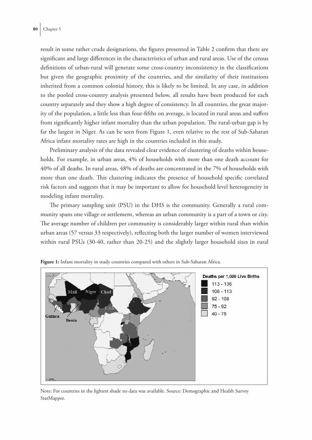
80 Chapter 5
result in some rather crude designations, the figures presented in Table 2 confirm that there are significant and large differences in the characteristics of urban and rural areas. Use of the census definitions of urban-rural will generate some cross-country inconsistency in the classifications but given the geographic proximity of the countries, and the similarity of their institutions inherited from a common colonial history, this is likely to be limited. In any case, in addition to the pooled cross-country analysis presented below, all results have been produced for each country separately and they show a high degree of consistency. In all countries, the great major-ity of the population, a little less than four-fifths on average, is located in rural areas and suffers from significantly higher infant mortality than the urban population. The rural-urban gap is by far the largest in Niger. As can be seen from Figure 1, even relative to the rest of Sub-Saharan Africa infant mortality rates are high in the countries included in this study.
Preliminary analysis of the data revealed clear evidence of clustering of deaths within house-holds. For example, in urban areas, 4% of households with more than one death account for 40% of all deaths. In rural areas, 48% of deaths are concentrated in the 7% of households with more than one death. This clustering indicates the presence of household specific correlated risk factors and suggests that it may be important to allow for household level heterogeneity in modeling infant mortality.
The primary sampling unit (PSU) in the DHS is the community. Generally a rural com-munity spans one village or settlement, whereas an urban community is a part of a town or city. The average number of children per community is considerably larger within rural than within urban areas (57 versus 33 respectively), reflecting both the larger number of women interviewed within rural PSUs (30-40, rather than 20-25) and the slightly larger household sizes in rural
Figure 1: Infant mortality in study countries compared with others in Sub-Saharan Africa.
Hoofdstuk 5 : Figure 1: Infant mortality in study countries compared with others in Sub-Saharan Africa.
Note: For co untries in the lightest shade no data was available. Source: Demographic and Health Survey StatMapper. Figure 2: Percentage contribution of each covariate to the rural-urban gap in infant mortality in the pooled sample.
Decomposition Model (1)
-10-505
10152025303540
first
born
birth
ord
er>4
mot
her's
age
at b
irth
shor
t birt
h in
terv
alm
othe
r's e
duca
tion
cont
race
ptio
nm
othe
r's a
ge a
t 1st
mar
riage
mal
e ch
ildag
e of
hou
seho
ld h
ead
mal
e ho
useh
old
head
toile
t
wat
erel
ectri
city
no fi
nish
ed fl
oor
asse
ts in
dex
unob
serv
ed h
h he
tero
heal
th fa
cilit
ies
publ
ic tr
ansp
ort
unob
serv
ed c
omm
het
ero
coun
try e
ffect
s
% c
ontri
butio
n
Note: For countries in the lightest shade no data was available. Source: Demographic and Health Survey StatMapper.

What explains the rural-urban gap in infant mortality —household or community characteristics? 81
areas. Within urban areas, 7% of deaths occur in the 1% of communities with 10 or more deaths; whereas within rural areas 49% of deaths are concentrated in the 22% of communities with 10 or more deaths. These numbers suggest that while there is clustering of infant deaths within communities, deriving from correlated risk factors at this level, the degree of concentra-tion is less pronounced than that within households, and is even less so within urban areas.
Explanatory variables
With respect to the proximate determinants, the DHS, like many other nationally representative datasets, only provide direct measures of what Mosley & Chen (1984) refer to as ‘maternal fac-tors’. We include mother’s age at birth, birth order and an indicator of short birth interval (<24 months). The effect of birth order is captured by a dummy for first born children and another for children with a birth order higher than four (Sastry 1997a; Rutstein 2000).
Maternal education is represented by a dummy variable indicating no or incomplete primary education. We further control for the social status and empowerment of the mother through her age at first marriage (Folasada 2000; Bhargava 2003), the sex of the household head (Lloyd & Blanc 1996; Canagarajah 2001) and the mother’s use of contraception (Birdsall & Chester 1987). Attitudes, traditions and social norms that may impact on investments in child health are further proxied by the sex of the child, to allow for the effect of discriminatory traditions, and the age of the head of household. Molbak et al (1997) found that children in households with a younger head are associated with higher diarrhea prevalence, a major contributor to infant mortality.
Exposure to environmental contamination is proxied by a dummy for household access to water from a safe source and another for availability of a toilet (see Table 1 for definitions) (Victora et al 2005). Further, we include information on the floor material of the household dwelling and whether the household has an electricity supply (Smith et al 2005). Housing mate-rials may act as a proxy for the quality of housing, exposure to vermin and overcrowding, which raises the risk of respiratory disease. Electricity facilitates more hygienic preparation of food and sterilization. While these indicators of environmental conditions are defined at the household level, they are clearly not independent from community level infrastructure (Sastry 1996). In fact, the between community variation in source of water and in electricity supply is larger than the within community variation. But the latter is still considerable. In communities where at least one household has safe water (electricity), only one-half (one-third) of all households have a supply. On the other hand, when at least one household does not have a safe source of water (electricity) over two-thirds (nine-tenths) of all households in the community are without a supply. Community level investments in infrastructure are necessary but not sufficient for households to have a safe supply of water or an electricity supply. Constraints and preferences at the household level also seem to be important.

82 Chapter 5
To obtain a proxy for wealth, beyond that indicated by access to drinking water, sanitation, electricity and housing materials, we construct an index using principal components analysis on possession of assets such as a car, motor, bicycle, radio, television, and refrigerator (Filmer & Pritchett 2001; Hong 2006). The first principal component is used to divide households into the poorest, middle and richest thirds.4
At the community level, we approximate the availability of health care services and public transport with dummies to indicate the presence of a health facility and any public transport respectively.5 Brenneman (2002) found evidence reported in various studies that better transport contributes to easier access to health care as well as easier staffing and operation of clinics. Moreover, improved transport policy can reduce air pollution in urban areas and increase the supply of food in rural ones.
Table 2 shows the means of all covariates across urban and rural areas. Children born in rural areas are at a disadvantage across virtually all health determinants. This is true for the pooled cross-country sample, as well as within each country.6
While the data allows us to measure many of the important determinants of infant mortal-ity, one might expect there to be considerable variation in survival chances across households and communities that is not captured by these covariates. In the next section we present a model of infant mortality that allows for household and community level effects and then show how the contribution of these effects to the rural-urban gap, as well as those of the observable factors, can be quantified.
4 Using such a list of assets for both urban and rural areas from a common set of assets may understate the wealth of rural households because the DHS generally contain more information on assets that are more common to urban areas (eg. refrigerator, television). Households in rural areas may have a range of resources that are often not recorded in DHS, like land, rights to fishing, gathering or grazing, or the space and resources to keep animals. It might also be that the correlation between certain assets and wealth differs between urban and rural areas, although Menon et al (2000) have found no clear evidence of this.
5 We also tried including other community variables such as the existence of a market place, but this showed no effect. Further, we experimented with creating an index of public services that combines information on existence of a shop, public transport, market, post, bank, and garbage collection in the community. However, these services were not consistently available for all countries and were not significant in country specific models. For some countries the data contain more detailed information on health services but proximity is the only information that is available across the entire set of countries.
6 When decomposing rural-urban gaps in infant mortality into gaps in the determinants, it is important to have sufficient ‘common support’ of the determinants across urban/rural areas. Otherwise, a covariate might be just picking up the rural-urban disparity, or might be capturing an ‘outlier’ effect. In this respect, Table 2 shows the very low average electricity access in rural areas. However, when we redid the entire analysis (also the country specific regressions) excluding the electricity variable, the effects of the other variables remained unchanged. Table 2 also illustrates the very low levels of maternal education in rural areas, which is why we could not discriminate further between higher education levels.

What explains the rural-urban gap in infant mortality —household or community characteristics? 83
Methods
Three-level random intercept probit model
We model the probability of infant mortality using a three-level probit model with random intercepts representing unobservable heterogeneity at both the household and the community level (Gibbons & Hedeker 1997). Compared to a standard probit, this model has the advantage of estimating the correlation in survival probabilities among children belonging to the same family and that among those residing in the same community that persists after controlling for observed characteristics (Sastry 1997b; Bolstad & Manda 2001). Failure to account for this unobserved heterogeneity would lead to inconsistent coefficients.7 An important assumption of any random-effects model is that the unobservable components at each level are uncorrelated with the observable covariates. This can be overly restrictive. For example, it rules out the pos-sibility that high birth order and short birth interval reflect previous infant deaths resulting from the same unobservable factors that condition the survival chances of all children in a household (Bhargava 2003). To allow for correlation between unobserved heterogeneity and observable characteristics, while still identifying the contribution of the latter, we adopt the Mundlak (1978) – Chamberlain (1980) approach of parameterizing the unobservable effects as functions of the means of the regressors at the next lowest level. The three-level random component probit model can then be written as:
85
*ihc
*
1 if y 0
with
ihc
ihc ihc hc c ihc
hc hc hc
c c c
y
y xxx
(1)
where *ihcy is a latent index the sign of which determines observation of an infant death
1ihcy , and the indices i, h and c refer to infants, households and communities
respectively. To simplify the notation we use ihcx to represent the entire vector of
covariates, but covariates can vary on child, household or community level. The
unobservable household ( hc ) and community level intercepts ( c ) are assumed to be a
function of the within household means of the child level covariates ( hcx ) and the within
community means of the household level covariates ( cx ) respectively. Conditional on
these means, the residual unobservable heterogeneity at each level ( hc and c ) is
assumed independent of the covariates. This exogeneity assumption is weaker than that in
the standard three-level random-effects probit model since the within household means,
for example, should absorb the effects of unobservables that impact both on infant
mortality and covariates across all individuals within the same household. The within
community means serve a similar purpose in absorbing effects common to infant
mortality and covariates across all households in the same community.
The idiosyncratic error term ihc is assumed to follow a standard normal
distribution. The random components at each level are assumed multivariate normal,
mutually independent and independent of the idiosyncratic error ihc . The assumption of
multivariate normality is standard in multi-level models.
The likelihood of the model can be written as:
(1)
where y*ihc is a latent index the sign of which determines observation of an infant death (yihc =1),
and the indices i, h and c refer to infants, households and communities respectively. To simplify the notation we use xihc to represent the entire vector of covariates, but covariates can vary on child, household or community level. The unobservable household (αhc ) and community level intercepts (αc ) are assumed to be a function of the within household means of the child level covariates (xhc ) and the within community means of the household level covariates (xc ) respectively. Conditional on these means, the residual unobservable heterogeneity at each level (ηhc and ηc ) is assumed independent of the covariates. This exogeneity assumption is weaker than that in the standard three-level random-effects probit model since the within household means, for example, should absorb the effects of unobservables that impact both on infant mortality and covariates across all individuals within the same household. The within community means
7 Neglecting unobserved heterogeneity in non-linear models causes coefficients to be inconsistent, although consistency of the average partial effects is preserved (Wooldridge 2002).

84 Chapter 5
serve a similar purpose in absorbing effects common to infant mortality and covariates across all households in the same community.
The idiosyncratic error term (εihc ) is assumed to follow a standard normal distribution. The random components at each level are assumed multivariate normal, mutually independent and independent of the idiosyncratic error (εihc ). The assumption of multivariate normality is standard in multi-level models.
The likelihood of the model can be written as:
86
1 1
| , , , , | , , | , ,cnn
ihc ihc hc c hc c hc ihc hc c hc c ihc hc c cc h
f y x x x x x x d x x x d
(2)
where
1,1
( , , , ) 1hc
ihcihcn
yyihc ihc hc c hc c ihc hc c hc c ihc hc c hc c
if y x x x x x x x x x
is the joint density of the dependent variable for all infants within a given household
conditional on the household and community effects as well as the observable
explanatory variables and their within household and within community means. () is
the normal cumulative density function, () represents the normal density function of the
random disturbances with variances standardized to unity, n indicates the number of
communities, cn denotes the number of households within any given community and hcn
the number of infants within a given household.
The ‘posterior’ (conditional) density function of the random components can be
calculated using Bayes’ Theorem. For the household component, this gives:
| , , , ,( , , )
| , , ,
| , , , ,
| , , , ,
ihc ihc hc c hc c hchc ihc ihc c
ihc ihc hc c c
ihc ihc hc c hc c hc
ihc ihc hc c hc c hc hc
f y x x xp y x
f y x x x
f y x x xf y x x x d
(3)
where p denotes the posterior density. Because of the assumed independence
between the household and community level random components and of each with the
covariates, ( , , , )hc ihc hc c c hcx x x and the marginal distribution of c appears in
both the numerator and denominator and so cancels out. Following from this, the
posterior means of the random household components are given by:
(2)
where
86
1 1
| , , , , | , , | , ,cnn
ihc ihc hc c hc c hc ihc hc c hc c ihc hc c cc h
f y x x x x x x d x x x d
(2)
where
1,1
( , , , ) 1hc
ihcihcn
yyihc ihc hc c hc c ihc hc c hc c ihc hc c hc c
if y x x x x x x x x x
is the joint density of the dependent variable for all infants within a given household
conditional on the household and community effects as well as the observable
explanatory variables and their within household and within community means. () is
the normal cumulative density function, () represents the normal density function of the
random disturbances with variances standardized to unity, n indicates the number of
communities, cn denotes the number of households within any given community and hcn
the number of infants within a given household.
The ‘posterior’ (conditional) density function of the random components can be
calculated using Bayes’ Theorem. For the household component, this gives:
| , , , ,( , , )
| , , ,
| , , , ,
| , , , ,
ihc ihc hc c hc c hchc ihc ihc c
ihc ihc hc c c
ihc ihc hc c hc c hc
ihc ihc hc c hc c hc hc
f y x x xp y x
f y x x x
f y x x xf y x x x d
(3)
where p denotes the posterior density. Because of the assumed independence
between the household and community level random components and of each with the
covariates, ( , , , )hc ihc hc c c hcx x x and the marginal distribution of c appears in
both the numerator and denominator and so cancels out. Following from this, the
posterior means of the random household components are given by:
is the joint density of the dependent variable for all infants within a given household conditional on the household and community effects as well as the observable explanatory variables and their within household and within community means. Φ() is the normal cumulative density function, () represents the normal density function of the random disturbances with variances standardized to unity, n indicates the number of communities, nc denotes the number of house-holds within any given community and nhc the number of infants within a given household.
The ‘posterior’ (conditional) density function of the random components can be calculated using Bayes’ Theorem. For the household component, this gives:
86
1 1
| , , , , | , , | , ,cnn
ihc ihc hc c hc c hc ihc hc c hc c ihc hc c cc h
f y x x x x x x d x x x d
(2)
where
1,1
( , , , ) 1hc
ihcihcn
yyihc ihc hc c hc c ihc hc c hc c ihc hc c hc c
if y x x x x x x x x x
is the joint density of the dependent variable for all infants within a given household
conditional on the household and community effects as well as the observable
explanatory variables and their within household and within community means. () is
the normal cumulative density function, () represents the normal density function of the
random disturbances with variances standardized to unity, n indicates the number of
communities, cn denotes the number of households within any given community and hcn
the number of infants within a given household.
The ‘posterior’ (conditional) density function of the random components can be
calculated using Bayes’ Theorem. For the household component, this gives:
| , , , ,( , , )
| , , ,
| , , , ,
| , , , ,
ihc ihc hc c hc c hchc ihc ihc c
ihc ihc hc c c
ihc ihc hc c hc c hc
ihc ihc hc c hc c hc hc
f y x x xp y x
f y x x x
f y x x xf y x x x d
(3)
where p denotes the posterior density. Because of the assumed independence
between the household and community level random components and of each with the
covariates, ( , , , )hc ihc hc c c hcx x x and the marginal distribution of c appears in
both the numerator and denominator and so cancels out. Following from this, the
posterior means of the random household components are given by:
(3)
where p( ) denotes the posterior density. Because of the assumed independence between the household and community level random components and of each with the covariates, ϕ(ηhc|xihc, xhc, xc, ηc) = ϕ(ηhc) and the marginal distribution of ηc appears in both the numerator and denominator and so cancels out. Following from this, the posterior means of the random household components are given by:
87
| , , , ,ˆ
| , , , ,
hc ihc ihc hc c hc c hc hc
hcihc ihc hc c hc c hc hc
f y x x x d
f y x x x d
(4)
Similarly the posterior means of the community component are given by:
1
1
| , , , ,ˆ
| , , , ,
c
c
n
c ihc ihc hc c hc c hc hc c ch
c n
ihc ihc hc c hc c hc hc c ch
f y x x x d d
f y x x x d d
(5)
The likelihood is maximized and the posterior means of the random components are
computed by adaptive quadrature using the GLLAMM program in Stata (Rabe-Hesketh
2002; Rabe-Hesketh et al 2005).
Decomposition
Rural-urban disparity in infant mortality rates can arise from differences in: a) the
distributions of observable determinants of infant mortality; b) the effects of those
determinants; c) the distributions of unobservable determinants. Blinder-Oaxaca type
decomposition can be used to quantify the relative importance of these three explanations
(Blinder 1973; Oaxaca 1973). In a standard decomposition, the difference in the mean
effects of unobservables is reflected in the difference in the intercepts of urban and rural
specific regressions. But these intercept differences are not particularly helpful in
pinpointing the source of rural-urban disparities in infant mortality since they provide no
information on the level at which unobservables operate. We provide a more detailed
explanation of the rural-urban disparity by quantifying the contribution of unobservable
determinants of infant mortality at both the household and community levels. This is
(4)
Similarly the posterior means of the community component are given by:

What explains the rural-urban gap in infant mortality —household or community characteristics? 85
87
| , , , ,ˆ
| , , , ,
hc ihc ihc hc c hc c hc hc
hcihc ihc hc c hc c hc hc
f y x x x d
f y x x x d
(4)
Similarly the posterior means of the community component are given by:
1
1
| , , , ,ˆ
| , , , ,
c
c
n
c ihc ihc hc c hc c hc hc c ch
c n
ihc ihc hc c hc c hc hc c ch
f y x x x d d
f y x x x d d
(5)
The likelihood is maximized and the posterior means of the random components are
computed by adaptive quadrature using the GLLAMM program in Stata (Rabe-Hesketh
2002; Rabe-Hesketh et al 2005).
Decomposition
Rural-urban disparity in infant mortality rates can arise from differences in: a) the
distributions of observable determinants of infant mortality; b) the effects of those
determinants; c) the distributions of unobservable determinants. Blinder-Oaxaca type
decomposition can be used to quantify the relative importance of these three explanations
(Blinder 1973; Oaxaca 1973). In a standard decomposition, the difference in the mean
effects of unobservables is reflected in the difference in the intercepts of urban and rural
specific regressions. But these intercept differences are not particularly helpful in
pinpointing the source of rural-urban disparities in infant mortality since they provide no
information on the level at which unobservables operate. We provide a more detailed
explanation of the rural-urban disparity by quantifying the contribution of unobservable
determinants of infant mortality at both the household and community levels. This is
(5)
The likelihood is maximized and the posterior means of the random components are computed by adaptive quadrature using the GLLAMM program in Stata (Rabe-Hesketh 2002; Rabe-Hesketh et al 2005).
Decomposition
Rural-urban disparity in infant mortality rates can arise from differences in: a) the distribu-tions of observable determinants of infant mortality; b) the effects of those determinants; c) the distributions of unobservable determinants. Blinder-Oaxaca type decomposition can be used to quantify the relative importance of these three explanations (Blinder 1973; Oaxaca 1973). In a standard decomposition, the difference in the mean effects of unobservables is reflected in the difference in the intercepts of urban and rural specific regressions. But these intercept differ-ences are not particularly helpful in pinpointing the source of rural-urban disparities in infant mortality since they provide no information on the level at which unobservables operate. We provide a more detailed explanation of the rural-urban disparity by quantifying the contribution of unobservable determinants of infant mortality at both the household and community levels. This is achieved by extending the non-linear decomposition of the group difference in a binary indicator proposed by Fairlie (2005) to a three-level random intercept probit model.
The rural-urban gap in average infant mortality can be decomposed as follows:
1 1
1 1
( ) ( )
( ) ( )
r u
u u
r r r r r u u u u uN Nr u ihc hc c hc c ihc hc c hc c
r ui i
u r u r u r u u u u u u u u u uN Nihc hc c hc c ihc hc c hc c
u ui i
x x x x x xY YN N
x x x x x xN N
β δ γ η η β δ γ η η
β δ γ η η β δ γ η η
Φ Φ − −
Φ Φ
−
∑ ∑
∑ ∑
(6)
where superscripts r and u indicate values of covariates/estimates obtained from the rural and urban samples of children respectively, Nr and Nu indicate the number of infants located in rural and urban areas respectively, refer to the coefficients from the pooled (urban and rural) model and k
j j = hc,c and k = r, u are the household and community specific posterior means of the random disturbances that are estimated from (4) and (5). The term in the first set of brackets represents the part of the rural-urban gap that is due to differences in the distributions of the observable determinants of infant mortality as well as the differences in the unobserv-able household and community level determinants. The term in the second brackets gives the

86 Chapter 5
gap due to differences in the effects of the observable determinants.8 The coefficients from the pooled (urban and rural) model are used to weight the differences in the x’s in the first term, and the urban distribution of x’s is used to weight differences in the coefficients in the second term.9
The gap can then be decomposed further into the contributions of each covariate, both through its distribution and its effect. However, we will focus on the contributions of differences in the distributions of covariates and random household and community effects since, as will become apparent below, differences in coefficients contribute only marginally to the explanation of the rural-urban gap in infant mortality. To illustrate how the contributions of differences in the distributions of particular covariates are identified, consider a simple case in which infant mortality is explained by two determinants, x1 and x2 , and Nr = Nu. The contribution of the difference in the distributions of x1 to the rural-urban gap is then equal to (Fairlie 2005)
0 1 1 2 21
0 1 1 2 2
1 ( )
( )
rN r r r r r rihc ihc hc c hc cr i
u r r r r rihc ihc hc c hc c
x x x xN
x x x x
β β β δ γ η η
β β β δ γ η η
Φ
−Φ
∑ (7)
Similarly, the contribution of x2 can be expressed as
0 1 1 2 21
0 1 1 2 2
1 ( )
( )
rN u r r r r rihc ihc hc c hc cr i
u u r r r rihc ihc hc c hc c
x x x xN
x x x x
β β β δ γ η η
β β β δ γ η η
Φ
−Φ
∑ (8)
Basically, the contribution of each variable to the gap equals the change in the average predicted probability of dying from replacing the rural distribution with the urban distribution of that variable while holding the distributions of the other variables constant.10
To quantify the contribution of the difference between rural and urban areas in the means of the unobservable household-level heterogeneity we have to take into account that, according
8 Strictly speaking the random intercepts are parameters to be estimated and so one logic would place them with the contribution of the difference in the coefficients in the decomposition. We prefer to place them with the covariate contribution since they essentially reflect differences in the distributions of determinants, albeit unobservable ones.
9 Several weighting alternatives have been suggested in the decomposition literature (see e.g. Neumark 1988; Oaxaca & Ransom 1994). Using the pooled coefficients as weighting factors for differences in the distribution of the covariates seems most justified in our case since neither the rural nor the urban model can be interpreted as the natural order from which the other deviates due to discriminatory behavior .
10 Unlike in the linear case, the independent contribution of a covariate depends on the values of the other covariates. This implies that the order of switching the distributions could affect the estimated contribution of each covariate. To check sensitivity, we experimented with randomizing the order of the switching of covariates as suggested by Fairlie (2005) and found that the results were very robust.

What explains the rural-urban gap in infant mortality —household or community characteristics? 87
to (1), this heterogeneity is a function of the means of the child level covariates xhc. It can be estimated by11
0 1 1 2 21
0 1 1 2 2
1 ( )
( )
rN u u r r r rihc ihc hc c hc cr i
u u u r u rihc ihc hc c hc c
x x x xN
x x x x
β β β δ γ η η
β β β δ γ η η
Φ
−Φ
∑ (9)
This contribution depends both on rural-urban differences in the means of random household level determinants
90
that, according to (1), this heterogeneity is a function of the means of the child level
covariates hcx . It can be estimated by29
0 1 1 2 21
0 1 1 2 2
1 ( )
( )
rN u u r r r rihc ihc hc c hc cr i
u u u r u rihc ihc hc c hc c
x x x xN
x x x x
) ) ) ) ) ) )
) ) ) ) ) ) ) (9)
This contribution depends both on rural-urban differences in the means of random
household level determinants ˆ ˆr uhc hc and on differences in determinants at this level
that are correlated with the covariates ˆ ˆr uhc hcx x . Finally, the contribution of the
difference in community-level heterogeneity is estimated in a similar way by:
0 1 1 2 21
0 1 1 2 2
1 ( )
( )
rN u u u r u rihc ihc hc c hc cr i
u u u u u uihc ihc hc c hc c
x x x xN
x x x x
) ) ) ) ) ) )
) ) ) ) ) ) ) (10)
Since in our case the urban sample is smaller than the rural, a random rural
subsample is drawn and matched with the urban sample on the basis of predicted
probabilities of dying (Fairlie 2005).30 Since the results depend on the specific subsample
that is drawn, the process is repeated 100 times and average results are reported.31
Regression estimates, as well as the random drawing of the rural subsample take
into account the sample weights that come with DHS data. Although the analysis has
been conducted for each country separately, here we only present results from a pooled
analysis across countries. In this, weights are adjusted for differences in population size
29 In the model, the probability of dying is a non-linear function (i.e the normal cumulative density) over the distribution of the household and community intercepts. In the decomposition, we approximate this probability by the non-linear function evaluated at the posterior means of these household and community intercepts. 30 Since we use sampling with replacement, some rural children may be more than once in the subsample that is used for the matching. The order of these ‘duplicate’ children is then randomized to match them with an urban child. 31 Increasing the number of replications further did not change decomposition results significantly.
and on differences in determinants at this level that are correlated with the covariates
90
that, according to (1), this heterogeneity is a function of the means of the child level
covariates hcx . It can be estimated by29
0 1 1 2 21
0 1 1 2 2
1 ( )
( )
rN u u r r r rihc ihc hc c hc cr i
u u u r u rihc ihc hc c hc c
x x x xN
x x x x
) ) ) ) ) ) )
) ) ) ) ) ) ) (9)
This contribution depends both on rural-urban differences in the means of random
household level determinants ˆ ˆr uhc hc and on differences in determinants at this level
that are correlated with the covariates ˆ ˆr uhc hcx x . Finally, the contribution of the
difference in community-level heterogeneity is estimated in a similar way by:
0 1 1 2 21
0 1 1 2 2
1 ( )
( )
rN u u u r u rihc ihc hc c hc cr i
u u u u u uihc ihc hc c hc c
x x x xN
x x x x
) ) ) ) ) ) )
) ) ) ) ) ) ) (10)
Since in our case the urban sample is smaller than the rural, a random rural
subsample is drawn and matched with the urban sample on the basis of predicted
probabilities of dying (Fairlie 2005).30 Since the results depend on the specific subsample
that is drawn, the process is repeated 100 times and average results are reported.31
Regression estimates, as well as the random drawing of the rural subsample take
into account the sample weights that come with DHS data. Although the analysis has
been conducted for each country separately, here we only present results from a pooled
analysis across countries. In this, weights are adjusted for differences in population size
29 In the model, the probability of dying is a non-linear function (i.e the normal cumulative density) over the distribution of the household and community intercepts. In the decomposition, we approximate this probability by the non-linear function evaluated at the posterior means of these household and community intercepts. 30 Since we use sampling with replacement, some rural children may be more than once in the subsample that is used for the matching. The order of these ‘duplicate’ children is then randomized to match them with an urban child. 31 Increasing the number of replications further did not change decomposition results significantly.
. Finally, the contribution of the difference in community-level heterogeneity is estimated in a similar way by:
0 1 1 2 21
0 1 1 2 2
1 ( )
( )
rN u u u r u rihc ihc hc c hc cr i
u u u u u uihc ihc hc c hc c
x x x xN
x x x x
β β β δ γ η η
β β β δ γ η η
Φ
−Φ
∑ (10)
Since in our case the urban sample is smaller than the rural, a random rural subsample is drawn and matched with the urban sample on the basis of predicted probabilities of dying (Fairlie 2005).12 Since the results depend on the specific subsample that is drawn, the process is repeated 100 times and average results are reported.13
Regression estimates, as well as the random drawing of the rural subsample take into account the sample weights that come with DHS data. Although the analysis has been conducted for each country separately, here we only present results from a pooled analysis across countries. In this, weights are adjusted for differences in population size (World Bank 2006), such that coun-tries with larger populations have relatively more influence and the results can be interpreted as being representative for the region.14
11 In the model, the probability of dying is a non-linear function (i.e the normal cumulative density) over the distribution of the household and community intercepts. In the decomposition, we approximate this probability by the non-linear function evaluated at the posterior means of these household and community intercepts.
12 Since we use sampling with replacement, some rural children may be more than once in the subsample that is used for the matching. The order of these ‘duplicate’ children is then randomized to match them with an urban child.
13 Increasing the number of replications further did not change decomposition results significantly.
14 It must be noted that when pooling across countries, the data is in fact organized on four levels: children, households, communities and countries. We chose to include fixed as opposed to random effects to capture country-specific characteristics. Because we only have 6 countries, fixed effects are straightforward to estimate and do not require the assumption of independence of the other covariates.

88 Chapter 5
Results
Regression results
The first column of Table 3 shows regression coefficients estimated from the pooled cross-country sample of the Mundlak-Chamberlain specification (1). The second and third column show similar coefficients for urban and rural subsamples. Since the dependent variable indicates whether the child died within its first year, a positive coefficient means an increased risk of death. All coefficients have intuitive signs. We find that all proximate determinants are very strongly related to infants’ survival. Firstborn children have a higher probability of dying within their first year while the opposite holds for children of a higher birth order (above four). The latter finding contradicts earlier results of e.g. Sastry (1997a) and Rutstein (2000), and appears to be attributable to taking account of correlated unobservable household level heterogeneity, which we will return to shortly. Children born to women younger than 20 years have worse survival chances than those born to women between 20 and 35 years. A short interval between succeeding births is correlated with an increased likelihood of infant death
Regarding the socioeconomic determinants, we find that maternal primary education re-duces the risk of infant mortality. The point estimate is larger in rural areas but the difference is not significant. Among the proxies for traditions, social norms and attitudes, only the familiarity with contraception and the sex of the child are significantly correlated with infant mortality. Children of women that have ever used contraception are more likely to survive, as are girls.
Table 3: Coefficients of probit models with random household and community effects.
model (1) without community means
Variables POOLED URBAN RURAL POOLED URBAN RURAL
firstborn 0.222*** 0.152*** 0.239*** 0.222*** 0.154*** 0.222***
birth order>4 -0.049* -0.025 -0.054* -0.049* -0.025 -0.049*
mother’s age at birth≤20 0.116*** 0.125** 0.114*** 0.116*** 0.124** 0.116***
mother’s age at birth>35 -0.018 0.026 -0.027 -0.018 0.027 -0.017
short birth interval 0.0975*** 0.086** 0.100*** 0.098*** 0.086** 0.098***
mother not completed primary education 0.1267*** 0.059 0.167** 0.117*** 0.059 0.117***
contraception -0.124*** -0.148*** -0.112*** -0.122*** -0.152*** -0.122***
mother’s age at 1st marriage 0.0038 -0.000 0.005 0.004 0.002 0.004
male child 0.079*** 0.057* 0.085*** 0.079*** 0.055* 0.079***
age of household head 0.001 0.001 0.001 0.001* 0.001 0.001*
male household head 0.047 -0.013 0.075* 0.057* -0.029 0.058*
toilet -0.028 -0.024 -0.026 -0.017 0.098* -0.017
water -0.081*** -0.124** -0.069** -0.085*** -0.096** -0.085***

What explains the rural-urban gap in infant mortality —household or community characteristics? 89
model (1) without community means
electricity -0.109** -0.021 -0.171* -0.130*** -0.036 -0.131***
no finished floor 0.030 0.128** -0.023 0.066** 0.128*** 0.066**
poorest third 0.000 0.107** -0.022 0.019 0.119** 0.019
middle third 0.001 0.052 -0.016 0.0120 0.095** 0.012
health facilities -0.042* -0.109*** -0.033 -0.048** -0.098*** -0.048**
public transport -0.020 0.027 -0.044 -0.023 0.026 -0.023
Benin 0.168*** 0.246** 0.134** 0.122*** 0.172** 0.122***
Chad 0.036 0.162** -0.023 0.025 0.112* 0.025
Guinea 0.243*** 0.238*** 0.231*** 0.221*** 0.206*** 0.221***
Mali 0.270*** 0.345*** 0.248*** 0.275*** 0.324*** 0.275***
Niger 0.221*** 0.247*** 0.204*** 0.202*** 0.177*** 0.202***
Household means
birth order>4 0.236*** 0.220*** 0.239*** 0.235*** 0.220** 0.235***
mother’s age at birth<20 0.236*** 0.197** 0.244*** 0.236*** 0.198** 0.236***
mother’s age at birth>35 -0.069 0.008 -0.088 -0.068 0.006 -0.068
short birth interval 0.990*** 0.946*** 0.997*** 0.991*** 0.951*** 0.991***
Community means
poorest third 0.143** 0.060 0.183**
middle third 0.082 0.257** 0.033
no finished floor 0.125** 0.016 0.161*
mother not finished primary education -0.098 0.019 -0.132
contraception 0.047 0.009 0.132
mother’s age at first marriage 0.001 0.017 -0.001
age of household head 0.001 0.000 0.000
sex of household head 0.066 -0.056 0.135
toilet 0.058 0.314*** 0.008
water 0.005 0.064 -0.007
electricity -0.008 -0.059 -0.108
constant -2.413*** -2.656*** -2.443*** -2.216*** -2.136*** -2.216***
variance of household effect 0.221*** 0.088*** 0.249*** 0.222*** 0.091*** 0.222***
variance of community effect 0.020*** 0.000 0.023*** 0.021*** 0.000 0.021***
joint test hh means (p value) 0.000 0.0000 0.000 0.000 0.000 0.000
joint test comm means (p value) 0.324 0.0805 0.197
Notes: Dependent variable is 1 if child died before first birthday. Analysis based upon data pooled across all countries and split by urban/rural. * p<.10, ** p<.05, *** p<.01. Bold coefficients indicate that they differ significantly between urban and rural model at the 10% level.

90 Chapter 5
Environmental conditions, in particular a safe source of drinking water, appear to be impor-tant determinants of infant mortality risks in both urban and rural locations. In the latter, the very few households with an electricity supply have a greatly reduced probability of infant death. In urban areas, the mortality risk is substantially higher among households living in premises with no finished floor. It seems likely that this characteristic identifies slum dwellings and the poor public health conditions found there. In rural areas, the majority of dwellings have no finished floor and this is not significantly correlated with mortality risk. Surprisingly, having a toilet is not significantly correlated with mortality risk in either urban or rural areas. Children in households with fewer assets face a greater risk of death in urban but not in rural areas. This is consistent with a greater socioeconomic gradient in child health in urban areas that has been found in other studies (Fotso 2006; Van de Poel et al 2007). Note that having controlled for the community means of these environmental and socioeconomic variables, the effects under discussion are identified from within community variation alone and are unlikely to be biased by correlated community level unobservables.
The existence of a health facility is correlated with a reduced risk of death but the effect is strongly significant only in urban areas. The lack of significance in rural areas may reflect the low quality of health services, with frequent absences of staff and medicines, or the lower probability of seeking health care in rural areas due to high opportunity costs and/or cultural sensitivity (Lavy et al 1996; Lalou & LeGrand 1997; Lindelouw & Serneels 2006; Say & Raine 2007). The availability of public transport is negatively correlated with infant mortality in rural areas, where presumably it is more crucial, but the effect is not significant in either sample.
The coefficients on household and community means of the child and household level covari-ates should be interpreted as reflecting the degree to which these variables are correlated with the unobserved household and community level heterogeneity respectively. Jointly the household level means are highly significant and all are individually significant but for the indicator of the mother being older than 35 at the time of birth. The inclusion of these household level means reduces the coefficient on the indicator of short birth interval and reverses the sign on birth order higher than four.15 As discussed in the Methods section, it is likely that short birth interval and high birth order reflect previous infant deaths, and therefore not only have a direct effect on survival chances, but are correlated with unobservable mortality risks that threaten all children born within a household. However, once this unobserved mortality risk is controlled for, having more siblings within the household can be beneficial for infant survival if, for example, these siblings can take up some child care responsibilities (Bhargava 2003).
The community means of the household level variables are not jointly significant in the pooled and rural samples and only weakly significant in the urban sample. Only the proportion of households with few assets and with no finished flooring is significantly correlated with the
15 Results without inclusion of the household level means are not presented but are available from the authors.

What explains the rural-urban gap in infant mortality —household or community characteristics? 91
unobserved community mortality risk. Counterintuitively, the proportion of households with satisfactory sanitation is positively correlated with community level mortality risk in urban areas. The joint insignificance of the community means indicates that household level covariates are not strongly correlated with unobservable community level risks and, consequently, that our model might be over parameterized. To check whether the decomposition results are overly influenced by many insignificant variables, we also conduct the analysis omitting the com-munity level means. The regression results are generally very robust to this exclusion – compare the first and last three columns of Table 3 – but for the expected increase in the magnitude of the coefficients on the few variables for which the community means are significant.
Conditional on the covariates and their household/community means, household level heterogeneity accounts for 18% of the remaining variance in infant mortality, whereas com-munity level heterogeneity, while significant, accounts for less than 2%. These results are robust to exclusion of the community means of household characteristics, a further indication that the community heterogeneity is uncorrelated with these covariates. The relative importance of the household level variance could be anticipated from the strong clustering of deaths by household discussed in the Data section. Curtis et al (1993) also found household heterogeneity explaining about 23% of the random variance in infant mortality in Brazil. However, another study of child survival (to age five rather than one) in Brazil that allowed for both household and community random effects found the latter to be more important (Sastry 1997b). The only other study of child survival that has allowed for both effects was of Malawi and this, like the present study, found household level heterogeneity to be more important (Bolstad & Manda 2001). Both household and community level heterogeneity are larger within rural areas. The community component is even absent within urban areas.
When using under-five instead of infant mortality, which almost doubled the number of deaths, we still found a very small estimate of community level variance. This suggests that the low community level variance is not just due to the smaller number of deaths in urban communities.16 Further, the community level variance did not increase much by omitting the household random effect, suggesting that there is not a problem of separately identifying the two effects. Finally, when we re-estimated the model omitting community level covariates, the community level variance did not increase by much suggesting that it is not the case that there is a large community level effect that is adequately captured by observable characteristics.
16 Using under-five instead of infant mortality increases the proportion of deaths and makes the unobserved components easier to identify. However to still have sufficient observations, it is required to extend the time period in which births took place (we used 15-5 years before the survey) and therefore it less likely that current household conditions reflect those within the first years of life.

92 Chapter 5
Decomposition results
The decomposition method (6) reveals that very close to 100% of the rural-urban gap in infant mortality can be explained by differences in the distributions of the covariates and the random effects and so, in aggregate, differences in the coefficients do not explain any of the gap. This does not mean that there are no differences in the effects of determinants of infant mortality across rural and urban areas. Rather, there are no systematic differences. Some determinants, such as electricity supply, have a stronger effect in rural areas, while others, such as wealth as in-dicated by possession of assets, have a stronger effect in urban areas. Given the limited evidence of significant rural-urban differences in coefficients and their zero net effect in aggregate, in the remainder of the analysis we focus on the contributions of differences in the distributions of observable and unobservable determinants of infant mortality.
In Table 4 we present the contribution of each covariate, computed analogously to (7)-(8), and of the unobservable household and community heterogeneity, estimated as in (9) and (10) respectively. Relative contributions are presented in Figure 2.17 We first discuss results generated from model (1), which includes both the household and community level means to capture correlated unobservable effects, and thereafter discuss robustness of the results when the com-munity means are omitted. It should be kept in mind that the contribution of a covariate reflects both the difference between the rural and urban distributions of that variable and the magnitude of its association with infant mortality as given in Table 3.
17 In these detailed decomposition results, the percentage of the gap that is explained does not exactly equal the 100 percent mentioned before. This is due to the approximation in the contribution of the unobservables mentioned in Footnote 11.
Figure 2: Percentage contribution of each covariate to the rural-urban gap in infant mortality in the pooled sample.
Hoofdstuk 5 : Figure 1: Infant mortality in study countries compared with others in Sub-Saharan Africa.
Note: For co untries in the lightest shade no data was available. Source: Demographic and Health Survey StatMapper. Figure 2: Percentage contribution of each covariate to the rural-urban gap in infant mortality in the pooled sample.
Decomposition Model (1)
-10-505
10152025303540
first
born
birth
ord
er>4
mot
her's
age
at b
irth
shor
t birt
h in
terv
alm
othe
r's e
duca
tion
cont
race
ptio
nm
othe
r's a
ge a
t 1st
mar
riage
mal
e ch
ildag
e of
hou
seho
ld h
ead
mal
e ho
useh
old
head
toile
t
wat
erel
ectri
city
no fi
nish
ed fl
oor
asse
ts in
dex
unob
serv
ed h
h he
tero
heal
th fa
cilit
ies
publ
ic tr
ansp
ort
unob
serv
ed c
omm
het
ero
coun
try e
ffect
s
% c
ontri
butio
n
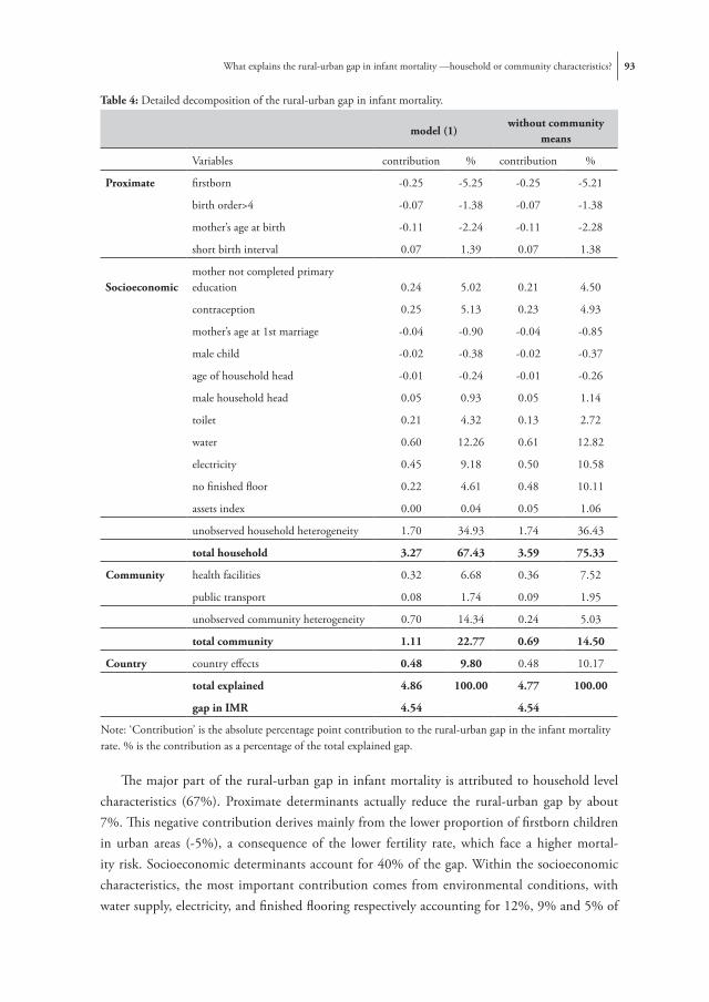
What explains the rural-urban gap in infant mortality —household or community characteristics? 93
The major part of the rural-urban gap in infant mortality is attributed to household level characteristics (67%). Proximate determinants actually reduce the rural-urban gap by about 7%. This negative contribution derives mainly from the lower proportion of firstborn children in urban areas (-5%), a consequence of the lower fertility rate, which face a higher mortal-ity risk. Socioeconomic determinants account for 40% of the gap. Within the socioeconomic characteristics, the most important contribution comes from environmental conditions, with water supply, electricity, and finished flooring respectively accounting for 12%, 9% and 5% of
Table 4: Detailed decomposition of the rural-urban gap in infant mortality.
model (1)
without community means
Variables contribution % contribution %
Proximate firstborn -0.25 -5.25 -0.25 -5.21
birth order>4 -0.07 -1.38 -0.07 -1.38
mother’s age at birth -0.11 -2.24 -0.11 -2.28
short birth interval 0.07 1.39 0.07 1.38
Socioeconomicmother not completed primary education 0.24 5.02 0.21 4.50
contraception 0.25 5.13 0.23 4.93
mother’s age at 1st marriage -0.04 -0.90 -0.04 -0.85
male child -0.02 -0.38 -0.02 -0.37
age of household head -0.01 -0.24 -0.01 -0.26
male household head 0.05 0.93 0.05 1.14
toilet 0.21 4.32 0.13 2.72
water 0.60 12.26 0.61 12.82
electricity 0.45 9.18 0.50 10.58
no finished floor 0.22 4.61 0.48 10.11
assets index 0.00 0.04 0.05 1.06
unobserved household heterogeneity 1.70 34.93 1.74 36.43
total household 3.27 67.43 3.59 75.33
Community health facilities 0.32 6.68 0.36 7.52
public transport 0.08 1.74 0.09 1.95
unobserved community heterogeneity 0.70 14.34 0.24 5.03
total community 1.11 22.77 0.69 14.50
Country country effects 0.48 9.80 0.48 10.17
total explained 4.86 100.00 4.77 100.00
gap in IMR 4.54 4.54
Note: ‘Contribution’ is the absolute percentage point contribution to the rural-urban gap in the infant mortality rate. % is the contribution as a percentage of the total explained gap.

94 Chapter 5
the gap. Maternal education also accounts for about 5% of the gap. Except for familiarity with contraception, which contributes 5%, all other proxies for traditions, social norms and attitudes do not contribute much.
Differences in household level unobserved heterogeneity contribute a substantial 35% to the gap. This is attributable to differences in the means of both uncorrelated and correlated unobservable household level determinants, with the contribution of the latter being identified from across household variation in individual level determinants.
Community characteristics contribute 23% to the gap, the most important contribution coming from the unobserved community heterogeneity (14%). The contribution of this hetero-geneity includes that of correlated effects identified through the across community variation in the means of household level variables. As discussed above, these means are jointly insignificant and their inclusion in the decomposition could result in an overestimate of the contribution of unobserved community level heterogeneity. To check this, we repeat the analysis omitting the community means of covariates from the model and decomposition. The contribution of com-munity level heterogeneity is indeed reduced, falling by almost two-thirds to 5% of the gap. But otherwise the results are quite robust to this restriction. The contribution of finished flooring doubles to reach 10% in relative terms, and that of asset ownership increases to 1%. Since it is only the means of these variables that are significant in the unrestricted model, there is evidence that they are correlated with unobservable community effects and that their contributions are biased upward when there is no control for this correlation. After taking account of the impact on the contributions of these two variables, the estimated contribution of community unob-served heterogeneity does not appear to be greatly inflated by the inclusion of many insignificant community means. In order to avoid overstating the contribution of any single variable, we suggest that greater weight be placed on the results from the more general model in which the contributions of household level covariates are identified from their within community variation alone and that of their across community variation is attributed to correlated unobservable community level determinants.
Existence of a health facility in the community accounts for 7% of the gap, and public trans-port contributes a further 2%. Note that interpretation of these effects as causal relies on the assumption that, conditional on the other covariates, including the community level means, the existence of a health facility and of public transport is uncorrelated with the residual community level heterogeneity. But even if this assumption does not hold, the two characteristics provide proxies for community level determinants and we still have an estimate of the rural-urban gap in infant mortality that is explained by differences at the community, as opposed to the household, level.
The contribution of the country effects amounts to 10% and is caused by two factors. First, there are differences across countries in the urban/rural population split (Table 2), and therefore the proportion of infants from any one country in the pooled sample differs across

What explains the rural-urban gap in infant mortality —household or community characteristics? 95
urban and rural areas. Second, infant mortality differs across countries even after controlling for all covariates (Table 3).
Country specific analysis
The relative importance of household versus community level determinants in explaining the rural-urban gap in infant mortality could differ across countries. To check this, we carried out the analysis for each country separately. In fact, there is a high degree of consistency in the results across countries and so we only comment on them briefly.18
As would be expected, and has been found elsewhere (Kuate-Defo & Diallo 2002), there is greater cross-country consistency in the effects of maternal characteristics than in those of socioeconomic factors. Notwithstanding the variation in the latter, the country-specific results generally confirm those from the pooled analysis. Unobserved household heterogeneity explains a substantial part of the random variance in infant mortality, ranging from 32% in Chad to 7% in Mali. The proportion of the random variance explained by the community component is again very small, being highest in Niger (2%) and insignificant in Benin, CAR, Guinea and Mali. In all countries, the decomposition shows that the major part of the rural-urban gap is caused by differences in the distributions of household determinants, with the major contribu-tions coming from household environmental characteristics (ranging from 48% in Chad to 15% in Guinea) and household level heterogeneity (ranging from 102% in Chad to 26% in CAR).
Conclusion
Our decomposition analysis has demonstrated that the rural-urban gap in infant mortality in six Central and West sub-Saharan African countries is explained by differences in the distributions of factors that determine mortality and not by differences in the effects of those determinants between rural and urban locations. Rural-urban differences in household level determinants, which explain two-thirds of the gap, are much more important than those in community level determinants, which explain less than a quarter.
At the household level, within the Mosley & Chen (1984) framework, proximate deter-minants of infant mortality – which in this paper mainly consist of maternal factors such as a short birth interval and birth order – are strongly and consistently related to infant survival. This is very much in line with previous research, e.g Sastry (1996) and Manda (1999). How-ever, because these determinants are very equally distributed across urban and rural areas (and
18 The country-specific results are available from the authors on request.

96 Chapter 5
because their effects are so consistent), they are not important in explaining the rural-urban infant mortality gap.
Our results confirm the previously established relations between infant mortality and socio-economic characteristics such as maternal education, familiarity with contraception and access to a safe water source. Since rural-urban differences in the distributions of these determinants are much larger than for the proximate ones, they are far more important in explaining the gap, accounting for around half of the household level contribution. Housing conditions and access to utilities play a particular strong role. We have identified the causal effects of these environmental factors only from their within community variation across households. This does not imply that the large contribution of environmental factors can only be influenced through policies that operate on household constraints and behavior. Access to sanitation, safe water and electricity is constrained first by the community level infrastructure and only second by the household’s means to make lower level investments in connecting to this infrastructure. The large contributions of water and electricity supply, together with the relatively large between-community variation they exhibit, suggest that investments in community infrastructure could potentially play an important role in narrowing differences in infant mortality. But the avail-ability of a water or electricity supply by itself does not ensure that all households are connected to it. Investments in the community infrastructure need to be combined with initiatives that help households take advantage of it.
Unobservable household level factors are as important as observable determinants in ex-plaining the rural-urban disparity in infant mortality, accounting for 35% of the gap. While the absolute contribution of unobservable heterogeneity at the community level is less (14%), it is larger relative to that of observable community level determinants. Allowing for unobserved heterogeneity in the decomposition is important not only because it reveals the contribution of unobservable household and community level determinants, but also because accounting for them provides better estimates of the contribution of the observed characteristics. We use household and community level means of observables to proxy the unobserved household and community level mortality risk respectively, and so make the exogeneity assumption of the three-level random- effects probit model more plausible. The results do indeed reveal depen-dencies between fertility related variables, such as a short birth interval and high birth order, and the unobserved household mortality risk. There is less evidence of correlation between the household level covariates and the unobservable community level mortality risks. However, in order to reduce the risk of overstating the importance of household relative to community level factors in explaining the rural-urban gap we have continued to use the between community variation in household characteristics to represent unobservable community level heterogeneity. This increases the robustness of our main result—that rural-urban differences in household characteristics are more responsible for the gap in infant mortality than those in community characteristics.

What explains the rural-urban gap in infant mortality —household or community characteristics? 97
Most of the contribution of observed community level factors is due to the lower proximity to health facilities in rural areas. The interpretation of this effect as causal relies upon the as-sumption that the within community means of household level factors are sufficient to absorb any effects common to infant mortality and access to health facility, as well as other covariates across all households in the same community. While if the assumption were not to hold the interpretation of the health facility effect would change, in the decomposition its contribution would remain at the community level, only now being counted as a proxy for unobservable heterogeneity. So either way, the decomposition quantifies the total contribution of community relative to household level determinants to the rural-urban gap in infant mortality rates.
In sum, we have shown that child survival in these countries depends first and foremost on the living conditions that constrain the ability of households to care for their children. Rural households do not behave so differently from their urban counterparts, but they live under conditions that are far more detrimental to their infants’ health. The decomposition reveals that the larger part of the rural-urban gap in infant mortality is caused by differences in household rather than community characteristics. This suggests that policies aiming to reduce the excess rural infant mortality need to operate not only through investments in community infrastructure and health programs but also by targeting the material needs of disadvantaged households within rural communities. Disadvantageous environmental conditions – such as limited electricity and water supply – contribute greatly to the rural-urban gap and derive both from a lack of community level infrastructure and from the inability of some households to exploit the infrastructure when it is available. In this respect, policy needs to operate at both the community and household levels to correct such deficiencies.


6Urbanization and the spread of diseases of affluence in China
We quantify, track and explain the distribution of overweight and of hypertension across Chinese provinces differentiated by their degree of urbanicity over the period 1991-2004. We construct an index of urbanic-
ity from longitudinal data on community characteristics from the China Health and Nutrition Survey and compute, for the first time, a rank-based measure of inequality in disease risk factors by degree of urbanicity. Prevalence rates of overweight and hyperten-sion almost doubled between 1991 and 2004 and these disease risk factors became less concentrated in more urbanized areas. Decomposition analysis reveals that one-half of the urbanicity-related inequality in overweight is directly attributable to community level characteristics, while for hypertension the contribution of such characteristics increased from 20% in 1991 to 62% in 2004. At the individual level, lower engagement in physical activity and farming explains more than half of the urban concentration of overweight and a rising share (28%) of the greater prevalence of hypertension in more urbanized areas. Higher incomes explain around one-tenth of the urban concentration of both overweight and hypertension, while the education advantage of urban popula-tions has a similar sized offsetting effect.

100 Chapter 6
Introduction
China is currently experiencing an urbanization process of remarkable scale. The percentage of the Chinese population living in urban areas increased from 27% in 1990 to 40% by 2005 (Na-tional Bureau of Statistics China 2006; UN 2007). By 2020, it is expected that this percentage will rise further to well over 50%, adding an additional 200 million mainly rural migrants to the current urban population of 560 million (UN 2007; Yusuf & Saich 2008). The consequences for population health are likely to be mixed. On the one hand, urban populations benefit from better access to health services, information and education, and have higher cash incomes and more economic opportunities (Liu et al 1999; Moore et al 2003). However, the rapid environ-mental, economic and social changes that follow urbanization increase the prevalence of major risk factors for chronic disease. In particular, urban areas in low and middle income countries are moving through a rapid nutritional transition towards Western-style diets, dominated by more processed foods and a higher fat content (Popkin 2001; Popkin & Du 2003). Increas-ing urbanization also leads to equally rapid shifts toward more sedentary occupations through the acquisition of new technology and transitions away from a mostly agricultural economy (Monda, Adair et al 2007). In China, these transitions have contributed to stark increases in the prevalence of conditions such as overweight and hypertension, especially amongst males, in urban areas and within high income groups (Liu et al 2004; Wang et al 2007; Weng et al 2007). The emergence of non-communicable diseases as a major health threat in countries still coping with infectious diseases and childhood malnutrition threatens to overstretch already struggling health services. Forecasts estimate that heart disease, stroke, and diabetes will cost China $556 in the period 2005–2015 (Wang et al 2005).
Increasing urbanization and development is likely to drastically change the geographical distribution of these non-communicable diseases. This paper investigates how the prevalence of overweight and hypertension varies across areas of China at different stages of urbanization, and how and why this spatial distribution is changing over time. In order to target public health interventions appropriately, it is important to establish whether these disease risk factors are spreading to less urban areas, or whether they are merely rising in the most urban ones. Knowledge of whether the geographic distribution of so-called diseases of affluence is changing because of changing population characteristics, behaviors or environmental factors is essential in identifying the type of interventions that are most likely to be effective in halting the spread of these diseases.
Analysis based on an urban-rural dichotomy does not adequately distinguish the different living and health conditions experienced in areas at different stages of urbanization (McDade & Adair 2001; Vlahov & Galea 2002; Champion & Hugo 2004; Dahly & Adair 2007). Further, there is no universally agreed definition of “urban” and “rural”, and in China the classification may have been influenced by the privileges to which non-agricultural residents were entitled

Urbanization and the spread of diseases of affluence in China 101
(Kojima 1995; Heilig 1999).1 New criteria for the designation of cities and towns were intro-duced in 1983, resulting in changes in the definition of urban administrative areas. These have necessitated changes in the census definition of the urban population from time to time, causing much confusion in counting the number of urban Chinese dwellers (Wu 1994; Shen 2006). Analysis of longitudinal survey data often presents a further problem in that the categorization of an area as urban or rural is fixed over survey waves. This is the case in the China Nutrition and Health Survey (CHNS) used here and so the dichotomous urban-rural variable does not capture the rapid urbanization of many designated rural areas that has occurred over the survey period.
To overcome these problems, we construct an urbanicity index using community data from the CHNS2. This index gives a ranking of communities from low to high levels of urbanicity, facilitating, for the first time in the urbanization literature, the use of rank-based measures of spatial inequality in overweight and in hypertension across areas at different stages of urbaniza-tion. We also use a decomposition method to explain what is driving these urbanicity-related inequalities in overweight and hypertension, and their trends over time. This method identifies the contribution of each determinant to inequality in the distribution of the disease risk factor by urbanicity, and makes clear that this contribution depends both on the urban concentration of the determinant and on the strength of its correlation with the risk factor. Changes can occur because the factors that determine overweight/hypertension are becoming more/less concen-trated in urban areas over time, or, for a given geographical distribution of the determinants, because their impact on overweight/hypertension is strengthening/weakening.
Data
This study uses data from the CHNS (http://www.cpc.unc.edu/projects/china), a large scale (and ongoing) longitudinal survey conducted in nine provinces of China in 1991, 1993, 1997, 2000 and 2004.3 The provinces represented in the survey are Liaoning, Shandong, Jiangsu, Henan, Heilongjiang, Hubei, Hunan, Guangxi and Guizhou (Figure 1). We have not included Heilongjiang in our analysis as this province only joined the CHNS in 1997. Although the
1 The administrative status of an area as ‘urban’ or ‘rural’ is very important since once classified as ‘urban’, residents become holders of urban registration (hukou) to whom the government is obligated to provide food, occupation, and accommodation (Kojima 1995). This way, there is an incentive for local governments to get areas recognized as being urban, which may obscure the meaningfulness of the classification.
2 Following McDade & Adair (2001) and Vlahov & Galea (2002), we use the term ‘‘urbanization’’ to describe the process by which communities become increasingly urban and the term ‘‘urbanicity’’ to describe the degree to which a community has the characteristics of an urban environment. Urbanization is a process, whereas urbanicity is a state at any point in time in that process.
3 In the 1989 survey, health and nutritional data were only collected from preschoolers and adults aged 20-45.

102 Chapter 6
CHNS is not a nationally representative sample, the provinces covered vary substantially in terms of geography and economic development. The bulk of the Chinese population is located in provinces in the eastern half of China, which are overrepresented in the CHNS, such that the selected provinces account for about 40% of the Chinese population (National Bureau of Sta-tistics China 2000). Since the pattern of city location in China has always been biased towards the East coast (Yan 1990), our sample is selected from the relatively more urbanized regions of China, although it does not include Beijing and Shanghai, the most urbanized areas in China (and among the most urbanized in the world). There is still substantial variation in urbaniza-tion rates across the CHNS provinces, ranging from 23% in Henan to 55% in Liaoning (in year 2000) (Shen 2006). Urbanization rates also vary considerably within each province. When interpreting our results, one must bear in mind that we investigate inequalities by urbanicity in the CHNS data, which are not necessarily the same as those for China as a whole.
The CHNS collects information on a wide range of individual socioeconomic, health and nu-tritional characteristics, and – essential for this study – also detailed information on community characteristics. A community, which is the primary sampling unit (PSU), is a government-designated administrative district.4 We examine the geographic distribution of disease risk
4 The community interview is held with the community head for questions related to public facilities and infrastructure, and with community health workers for questions related to health care provision.
Figure 1: Map of CHNS provinces, colored according to their average urbanicity index in 1991 and 2004.
Hoofdstuk 6: Figure 1: Map of CHNS provinces, colored according to their average urbanicity index in 1991 and 2004.

Urbanization and the spread of diseases of affluence in China 103
factors by urbanicity in the first and last available wave of the CHNS and the change in the distribution that occurred over the intervening 13 year period. Our sample consists of 6484 adults (aged 16 years and older) from 189 communities in 1991 and 6197 individuals from 192 communities in 2004. So, there are approximately 45 observations per community.5
The health indicators of interest are overweight and hypertension, both defined as binary indicators. Individuals are considered hypertensive if their average of three systolic blood pres-sure measurements was equal to or greater than 140 mm Hg and/or average diastolic blood pressure was equal to or greater than 90 mm Hg and/or they were taking medication to lower blood pressure (Sixth report of the Joint National Committee on the Detection, Evaluation, and Treatment of Hypertension 1997). Results are robust to not taking into account whether individuals were taking blood pressure lowering medication. Overweight is defined as a Body Mass index (BMI), based upon measured height and weight at the time of survey, above 25 kg/m2. This is the conventional BMI threshold for the definition of overweight and has also been recommended by the International Obesity Task Force (International Diabetes Institute 2000) as the appropriate definition of obesity in Asian populations on the basis of evidence that the health risks associated with obesity occur at a lower BMI in Asian populations (Shiwaku et al 2004). While other studies of Asian populations have referred to a BMI above 25 as “obesity” (Bell et al 2004; Monteiro et al 2004), we use the more conservative label of “overweight”.
In categorizing determinants of overweight and hypertension to be used to explain urban-icity-related inequality in the prevalence of these conditions, we have followed the conceptual framework proposed by Northridge et al (2003) who distinguish between factors at the macro, community and individual levels relevant to the association between urbanicity and population health. On the macro level, the framework includes the natural environment, social factors, and inequalities (in the distribution of wealth, educational and employment opportunities, and political influence). Most relevant for both overweight and hypertension are environmental factors, such as soil quality, minerals and climate that may impact on these conditions through diet.6 Given such factors are relatively fixed over time; we can capture them through a set of province dummies in our regression models.
These macro level factors, in turn, influence two domains of intermediate (community level) factors: the built environment and the social context (Table 1). We consider these community level determinants, which are very similar to those used in other studies (Liu et al 2003; Monda,
5 Note that we do not use the balanced panel data. Only keeping those individuals that are both in the 1991 and 2004 survey would limit sample size and would cause this sample to be much less representative. In turn, the urbanicity-related inequalities would only be meaningful for individuals in the panel.
6 Many studies have documented the higher prevalence rates of overweight/obesity and hypertension in the Northern regions of China, which seem to be associated with the higher salt intake and lower intake of fresh fruits and vegetables, as well as the colder weather in the north than in the south (He et al 1995; Wu et al 1995; Zhao et al 2004; Weng et al 2007).

104 Chapter 6
Table 1: Description of community characteristics used in the estimation of the urbanicity index, classified according to the framework proposed by Northridge et al (2003).
Category Variable Description
built envi-ronment
land use farmland 1 if there is any farmland in the community (0 otherwise)
agricultural workers % of community workforce working in agriculture (%)
transpor-tation
bus station 1 if community is near a bus station (0 otherwise)
train station 1 if community is near a train station (0 otherwise)
dirt roads 1 if dirt is main characteristic of roads in community (0 o/w)
gravel roads 1 if stone/gravel is main characteristic of roads in community
tarmac roads 1 if tarmac is main characteristic of roads in community
any tarmac road 1 if there is any tarmac road in community (0 otherwise)
distance to tarmac distance from community to nearest tarmac road (km)
services
distance to market average (over goods) distance to market (km)
telephone1 if community has convenient telephone service (0 otherwise)
post office 1 if there is a post office in community (0 otherwise)
newspaper1 if community can receive newspaper on the day it is published
primary school 1 if there is a primary school in the community (0 otherwise)
secondary school1 if there is a secondary school in the community (0 otherwise)
vocational school1 if there is a vocational school in the community (0 otherwise)
distance to health care
average distance to different types of health care facilities (km)
power cutaverage number of days per week that electricity is cut off (days)
childcare <3 years if there is a child care center for children <3 years old (0 o/w)
childcare <6 years if there is a child care center for children <6 years old (0 o/w)
restaurants number of restaurants in community
socio-economic context
enterprises number of enterprises in community
workers in large firms
% of workforce that is working in enterprises with >20 people
workers in small firms
% of workforce that is working in enterprises with <20 people
open trade area if there is an open trade area in community (0 otherwise)
population population of community

Urbanization and the spread of diseases of affluence in China 105
Adair et al 2007), as reflecting the urbanicity of a community. We have tried including more detailed information on health facilities, but as the coding of health facilities did not appear consistent across waves, we could only use availability of a health facility within the community. Further, we did not include population density of the community in the set of intermediate fac-tors because this information is missing for about 15% of the pooled sample of communities.7 However, since density is considered an important aspect of urbanicity, we have checked and confirmed the robustness of our results to including density and reducing the sample size. Any discrepancies are noted in the discussion of the results below.
On the lower, individual level Northridge et al (2003) consider what they refer to as proximate determinants, which consist of stressors, social integration and social support and health behav-iors.8 These are individual level demographic, socioeconomic and health behavior characteristics which directly or indirectly affect the probability of being overweight/hypertensive. In this set of determinants (Table 2) we include age-gender dummy variables, which allow the relationship between age and overweight/hypertension to vary across gender. Several studies have found the risk of overweight/obesity to increase with age, especially among women (Reynolds et al 2007; Hou 2008). Rates of hypertension in China have been found to be somewhat higher in men than women at younger ages, while the reverse is true at older ages (Wu et al 1995; Hou 2008). We also include marital status and a set of lifestyle variables: performance of heavy or very heavy physical activity, average daily fat intake, smoking status and whether the respondent consumes alcohol on a daily basis. Nutrient intake variables are calculated by the CHNS team based upon detailed food intake information regarding three days before the survey. We use fat intake as this better reflects dietary preferences than calorie intake (Lukman et al 1998).9 Reynolds et al (2007) and Hou (2008) found that smoking, alcohol consumption and physical activity are the most important factors explaining regional differences in both obesity and hypertension in China. Also considerable evidence points to the importance of the transition from the Chinese low fat diet to the high fat diet of the West in explaining the increasing obesity and hypertension rates (Lukman et al 1998). While smoking has severe adverse health effects, and increases blood
7 To use as much information as possible in the estimation of the urbanicity index, we use data of all waves (1991, 1993, 1997, 2000 and 2004). Calculation of population density requires data on population and area size. Unfortunately, information on the area size of the community was not collected in 1997 and 2000. In 2004, information on the size of the community was gathered retrospectively for all previous waves and so is only available for the balanced panel.
8 The term ‘proximate determinants’ is usually restricted to factors that have a direct impact on health, while ‘socioeconomic determinants’ are assumed to operate through these (e.g. Mosley & Chen 1984). For this reason, we refer to ‘individual level’, rather than ‘proximate’, determinants. Note, however, that one of these (income) is at the household level.
9 When both fat and calorie intake are included in the regression analysis, the latter is never a significant determinant of the probability of being overweight and it does not make a significant contribution to urbanicity-related inequality in the prevalence of overweight.

106 Chapter 6
pressure, it is associated with lower levels of obesity (Ueshima et al 2000; Chou et al 2004; Hou 2008).
The associations between socioeconomic status (measured by income and education) and both obesity and hypertension have been found to differ according to the level of development. Generally, overweight tends be more prevalent amongst the poor in high-income countries, whereas the reverse holds for low income countries (Wang 2001; Kim et al 2004; Reynolds et al
Table 2: Description of individual (household) level variables.
Category Variable Description
socioeconomic status
log incomelog of real household annual income divided by square root of household size (Yuan)
no education 1 if respondent has had no education (0 otherwise)
primary education 1 if respondent’s highest education is primary level (0 otherwise)
secondary education 1 if respondent’s highest education is secondary level (0 otherwise)
higher education 1 if respondent’s highest education is higher level (1-0)
not working 1 if respondent is not working (0 otherwise)
professional 1 if respondent is in a professional occupation (0 otherwise)
farmer 1 if respondent is a farmer (0 otherwise)
skilled worker 1 if resondent is a skilled worker (0 otherwise)
non-skilled worker 1 if respondent is a non-skilled worker (0 otherwise)
other work 1 if respondent is engaged in any other type of occupation (0 otherwise)
lifestyle
physical activity1 if respondent performs heavy or very heavy physical activity in daily activities
log fat intake logarithm of average daily gramms of fat intake
smoker 1 if respondent is currently smoking (0 otherwise)
alcohol 1 if respondent consumes alcohol on a daily basis (0 otherwise)
demographics
Male 16-29 1 if male aged 16-29 (0 otherwise)
Male 30-44 1 if male aged 30-44 (0 otherwise)
Male 45-64 1 if male aged 45-64 (0 otherwise)
Male 65+ 1 if male aged 65 plus (0 otherwise)
Female 16-29 1 if male aged 16-29 (0 otherwise)
Female 30-44 1 if female aged 30-44 (0 otherwise)
Female 45-64 1 if female aged 45-64 (0 otherwise)
Female 65+ 1 if female aged 65 plus (0 otherwise)
married 1 if respondent is married (0 otherwise)
Note: Underlined variable is the reference category.

Urbanization and the spread of diseases of affluence in China 107
2007). However, Monteiro et al (2004) have found that overweight in the developing world is not only a problem of the rich, and that, especially in middle income countries such as China, the burden of overweight is shifting over time towards the groups with lower socioeconomic status.
For socioeconomic status, we include a set of dummy variables for education level and (log) annual household income. The latter is calculated by summing all market earnings across the household and then adding the total value of all other non-market goods and services produced within that household (Figure 1 in Liu et al (2008) for the breakdown of household income into its various components). Household income is then deflated using a year/province/urban-rural specific consumer price index that was developed for use with the CHNS10, and divided by the square root of the total number of household members to obtain equivalent real household income per person.
Further, we control for individuals’ economic activity and occupation. More sedentary occu-pations such as office work are associated with an increased risk of overweight and hypertension as opposed to being involved in farming (Monda, Adair et al 2007).
In the Northridge et al (2003) conceptual framework, the community level variables have an impact on overweight/hypertension rates through individual level determinants, which are the direct causes of the conditions. The probability of suffering from overweight/hypertension de-pends directly on the individual’s genetic predisposition, diet, work and lifestyle, and indirectly on environmental factors that affect health-related behavior, such as the nature of the economy and so work, relative prices of food, advertising of convenience foods and the availability of fast food outlets. Hence, we include the urbanicity index among the set of covariates in the regression models explaining overweight/hypertension rates.
Calculating and validating the urbanicity index
Index construction
The concept of an urbanicity index was introduced in 1976 by Allen, and since then there have been attempts to develop an index from community level survey data. McDade & Adair (2001) use factor analysis on data from the Philippines, while Dahly & Adair (2007) assign weights to various community variables from the same data. For China, Liu et al (2003) create an index by weighting various community characteristics. Recently, Ng et al (2009) explored the different dimensions of urbanization in China by grouping sets of community and household
10 For more information see http://www.cpc.unc.edu/projects/china/data/datasets/convar.html. This is the income measure (and deflator) that is used by Liu et al (2008). We also checked robustness of the results when using GDP deflators for all China from the World Development Indicators (World Bank 2007).

108 Chapter 6
characteristics and assigning weights using CHNS data. In all these cases, the main motivation for constructing an index was to detect heterogeneity in degrees of urbanicity within the broad urban/rural dichotomy.
This paper applies factor analysis to a set of community level characteristics that reflect a community’s level of urbanicity. We prefer using factor analysis to weight the various compo-nents, as opposed to doing so subjectively, as this implies that the weights are chosen so as to maximize the explained variance in the underlying latent index.
Although we measure urbanicity-related inequality in 1991 and 2004 only, we use data from these and all the intervening waves to estimate the factor loadings of the urbanicity index. Doing so provides more information, allowing the factor loadings to be estimated with greater accuracy.11 These time-constant factor loadings are combined with the wave-specific values of a community’s characteristics to give a measure its degree of urbanicity at a point in time relative to that over all communities and waves. Table 3 shows summary statistics for the community variables across all waves from 1991 to 2004. Most variables show a trend that one would normally associate with increasing urbanicity: more communication and transportation pos-sibilities, a move away from agriculture, more economic activity and more community services such as schooling and child care. The mean population of a community more than doubled from 2248 in 1991 to 4933 in 2004. There is an apparent temporary reverse of this trend between 1993 and 1997 but this is not statistically significant.
To estimate the urbanicity index, we use factor analysis on this entire set of community characteristics (using the principal-factor method).12 We retain the first factor, which we assume to reflect the urbanicity of a community. This first factor explains the highest proportion of the common variance among the community variables, which in our case amounts to 47%. Factor loadings, reflecting the degree to which the variables are correlated with this first factor, are pre-sented in Table 4. They range between -1 and +1 with larger absolute values indicating a greater correlation. All of these loadings appear to have intuitive signs. Urbanicity is inversely associated with farming, bad road infrastructure, distance to markets and health facilities, and electricity cut-offs. The negative association with availability of a primary school is counter-intuitive, but also very weak. By contrast, urbanicity correlates positively with more transport infrastructure,
11 Admittedly, by pooling the data and ignoring the fact that there are repeated observations on communities we do not exploit all of the available information and so do not obtain an efficient estimator of the factor loadings. But for our purpose of ranking communities by degree of urbanicity, it is judged that the pooled data estimator will be sufficiently accurate.
12 Another option would be to use principal component analysis, which assumes that all variability in an item should be used in the analysis, while in principal factors analysis we only use the variability in an item that it has in common with the other items. Principal components analysis is often preferred as a method for data reduction, while principal factors analysis is often preferred when the goal of the analysis is to detect structure. Sahn & Stifel (2000) argue that factor analysis is more suited if one wishes to extract only 1 factor. In most cases, these two methods usually yield very similar results, and this was also confirmed in our study

Urbanization and the spread of diseases of affluence in China 109
communication services, schools, child care facilities, and economic activity.13 The urbanic-ity index is then constructed as a linear combination of all these community characteristics weighted by their factor loading (using an oblique promax rotation).14
13 The factor loadings are robust to including population density in the analysis, in which case the sample size is reduced (see note 7). Population density itself has a factor loading of 0.29 (detailed results available from the authors).
14 Values of the index are available from the authors on request.
Table 3: Summary statistics of intermediate (community) variables across waves.
Variable 1991 1993 1997 2000 2004
farmland 0.61 0.60 0.59 0.52 0.55
agricultural workers 47.27 42.70 41.30 39.24 32.95
bus station 0.55 0.54 0.62 0.69 0.63
train station 0.19 0.19 0.17 0.19 0.23
dirt roads 0.27 0.23 0.21 0.15 0.07
gravel roads 0.23 0.23 0.21 0.19 0.23
tarmac roads 0.50 0.55 0.58 0.66 0.70
any tarmac road 0.86 0.88 0.89 0.93 0.98
distance to tarmac 0.61 0.27 0.32 0.08 0.03
distance to market 1.03 0.86 0.80 0.23 0.22
telephone 0.56 0.66 0.81 0.93 0.89
post office 0.84 0.88 0.88 0.88 0.82
newspaper 0.31 0.39 0.49 0.46 0.59
primary school 0.66 0.73 0.72 0.77 0.72
secondary school 0.29 0.32 0.33 0.32 0.35
vocational school 0.07 0.09 0.09 0.09 0.09
distance to health care 5.35 3.22 4.62 4.10 2.90
power cut 1.20 0.87 0.60 0.47 0.31
childcare <3 years 0.20 0.21 0.28 0.24 0.32
childcare <6 years 0.45 0.48 0.54 0.43 0.54
restaurants 5.04 6.23 7.10 8.98 10.95
enterprises 36.73 32.38 40.23 97.95 174.81
workers in large firms 32.08 29.80 27.61 30.40 31.33
workers in small firms 8.41 10.38 15.99 18.35 17.09
open trade area 0.22 0.41 0.38 0.43 0.52
population 2247.98 2746.67 2256.70 3524.06 4932.85
Observations 189 181 167 191 192

110 Chapter 6
Assessing index reliability and validity
Internal consistency refers to the degree of interrelatedness of the items within the scale (DeVel-lis 2003) and is implied by using factor analysis, which maximizes the amount of explained variance in the underlying latent index.
Temporal stability: If the urbanicity index is representative of the underlying latent vari-able, then it should consistently assess that latent construct at different points in time (DeVellis 2003). As we can safely hypothesize that Chinese communities have become increasingly urban
Table 4: Factor loading for intermediate (community) variables
variable factor loading
farmland -0.65
agricultural workers -0.73
bus station 0.30
train station 0.23
dirt roads -0.62
gravel roads -0.27
tarmac roads 0.72
any tarmac road 0.45
distance to tarmac -0.21
distance to market -0.33
telephone 0.45
post office 0.20
newspaper 0.46
primary school -0.03
secondary school 0.21
vocational school 0.25
distance to health care -0.24
power cut -0.27
childcare <3 years 0.43
childcare <6 years 0.33
restaurants 0.47
enterprises 0.37
workers in large firms 0.46
workers in small firms 0.28
open trade area 0.27
population 0.29
Note: Factor analysis is used upon data pooled across all waves (1991, 1993, 1997, 2000 and 2004).

Urbanization and the spread of diseases of affluence in China 111
over the past decades, we expect our urbanicity index to increase over the waves of the CHNS as well. This is indeed confirmed: the average urbanicity index increases from -0.32 in 1991 to -0.13 in 1993, -0.07 in 1997, 0.09 in 2000 and 0.40 in 2004.
Criterion-related validity depends on the empirical association of the index with a ‘‘gold standard’’ (DeVellis 2003). Although we have no such gold standard of urbanicity, we can gain some insight into criterion related validity by investigating how the index correlates with the classification of each community as urban, suburb, town or rural by the CHNS interviewer in each wave. Figure 2 shows that our index does well in picking up different degrees of perceived urbanicity. Urban areas and towns have the highest average urbanization score, followed by sub-urban and rural areas. However, suburban areas clearly do not come second on the continuum from urban to rural. Figure 2 illustrates that all areas have become more urban during the respective time period, at a more or less equal pace. By 2004, there is no remaining difference in average urbanicity between towns and urban areas. This indicates that the infrastructure and services included in the urbanicity index have become equally likely to be present in towns as in urban areas. This suggests that our urbanicity index does not contain variables that can distinguish between communities located in highly urbanized areas (megacities) and those in towns with good infrastructure. The upper panel of Figure 1 displays the average value of the ur-banicity index for each CHNS province in 1991. The ranking of the provinces by these average scores almost exactly corresponds to that estimated by Shen (2006, table 6)15, which provides further support for the criterion-related validity of the index. The increase in urbanization over
15 Shen (2006) estimates urbanization rates only at the province level, using information on the urban/rural registration (hukou) of the population. Given the magnitude and heterogeneity of Chinese provinces, these aggregate rates would not be useful for our purpose of exploring how health varies with the degree of urbanicity households are exposed to.
Figure 2: Time trends in urbanicity index across the defined set of settlement classifications as available in the CHNS.
Figure 1: Map of CHNS provinces, colored according to their average urbanicity index in 1991 and 2004.
-1-.5
0.5
1ur
bani
city
inde
x
1991 1993 1997 2000 2004survey year
urban suburb town rural
Figure 2: Time trends in urbanicity index across the defined set of settlement classifications as available in the CHNS. Note: Based upon data pooled across all waves (1991, 1993, 1997, 2000 and 2004).
Note: Based upon data pooled across all waves (1991, 1993, 1997, 2000 and 2004).

112 Chapter 6
time is evident from Figure 1. The highest level of urbanization in 1991 corresponded to the lowest level by 2004.
Construct validity refers to the (theoretical) relationship between the urbanicity index and other variables (DeVellis 2003). We investigate this by examining the distribution of overweight, hypertension, fat intake and income across the distribution of the urbanicity index. Previous studies have found all of these variables to be more concentrated in urban areas and we confirm this in relation to quintiles of the urbanization index (Table 5).
Table 5: Percentages of sample overweight and hypertensive, and means of daily fat intake and annual real household income per person across quintiles of the urbanicity index
Quintiles of urbanicity index
least urban
second least urban
middlesecond most urban
most urban
% overweight 10% 12% 17% 25% 26%
% hypertensive 12% 14% 16% 21% 25%
daily fat intake (grams) 58.2 64.9 67.1 75.9 81.8
annual household income per person (Yuan) 1526 2293 2842 3431 4587
Notes: Statistics calculated from data pooled across all five waves of CHNS, 1991-2004. Income defined as in Table 2.
Added value of the urbanicity index
The distribution of the urbanicity index is presented in Figure 3 separately across areas labeled as urban and across those labeled rural within the CHNS. On average, urbanicity is much
Figure 3: Kernel density estimates of the urbanicity index for urban/rural communities as defined in the CHNS.
0.2
.4.6
.8ke
rnel
den
sity
urb
anic
ity in
dex
-2 0 2
kernel density for urban kernel density for rural
Figure 3: Kernel density estimates of the urbanicity index for urban/rural communities as defined in the CHNS. Note: Based upon data pooled across all waves (1991, 1993, 1997, 2000 and 2004).
0.2
.4.6
.81
cum
ulat
ive
prop
ortio
n of
ove
rwei
ght i
ndiv
idua
ls
0 .2 .4 .6 .8 1
Cumulative proportion of sample ranked by urbanicity
19912004diagonal
(a)
Figure 4a: Concentration curves illustrating distribution of overweight individuals by urbanicity in 1991 and 2004
Note: Based upon data pooled across all waves (1991, 1993, 1997, 2000 and 2004).

Urbanization and the spread of diseases of affluence in China 113
higher in communities classified as urban (mean index=0.52) than in those classified as rural (mean=-0.25). However, the overlap in the distributions illustrates that there is indeed substan-tial heterogeneity in urbanicity within the urban/rural administrative categories. The range of the index in communities classified as urban is [-1.7, 2.08], while it is [-2.50, 2.50] in ‘rural’ communities. Overall, 17% of ‘urban’ communities fell at or below the median urbanicity score across all waves, while 51% of ‘rural’ communities lay above it.
In sum, our urbanicity index appears to be a plausible indicator of the degree of urbanicity of a community. It shows the expected time trends, correlates well with the categorical classifica-tion and the urban/rural dichotomy but, importantly, it also reveals heterogeneity within the categories. In addition, unlike the static urban-rural dichotomy, the urbanicity index enables us to track the – often dramatic – changes in the communities’ environments over time.
Measurement and decomposition of urbanicity-related inequality in health
Measurement
Following Wagstaff et al (1991), the concentration curve and index have been popular tools for assessing socioeconomic inequalities in health. Given these are rank-based measures of inequality, they can also be used to assess urbanicity-related inequality with ranking provided by the urbanicity index. We use this approach to measure the degree to which overweight and hypertension are disproportionately concentrated among individuals located in more urbanized areas.
A concentration curve plots the cumulative proportion of the sample ranked from the least to the most urban according to the urbanicity index against the cumulative proportion of overweight (hypertensive) individuals. If there is no inequality, the curve will trace the 45o line. The concentration index (CI) is equal to twice the area between the concentration curve and the line of equality. A positive (negative) concentration index means that the health outcome is more (less) prevalent among people living in more urban areas.16 When applied to binary indicators such as overweight and hypertension, the bounds of the concentration index depend upon the mean of the indicator (Wagstaff 2005). This impedes comparisons over time due to substantial differences in means across survey years. Average prevalence rates of overweight and hypertension have almost doubled over the period 1991-2004. In 1991, 13% of our sample was obese and 14% hypertensive, while by 2004 these percentages have risen to 26% and 23%, which illustrates the fast rising threat of chronic diseases in China. To avoid dependency of the
16 It is important to note that, as opposed to income-related inequalities, urbanicity-related inequalities are not necessarily undesirable if these would result from purely geographical reasons

114 Chapter 6
CI bounds on the mean, we use an adjusted index suggested by Wagstaff (2005). This normal-ized concentration index is calculated as17:
117
A concentration curve plots the cumulative proportion of the sample ranked
from the least to the most urban according to the urbanicity index against the
cumulative proportion of overweight (hypertensive) individuals. If there is no
inequality, the curve will trace the 45o line. The concentration index (CI) is equal to
twice the area between the concentration curve and the line of equality. A positive
(negative) concentration index means that the health outcome is more (less) prevalent
among people living in more urban areas.16 When applied to binary indicators such as
overweight and hypertension, the bounds of the concentration index depend upon the
mean of the indicator (Wagstaff 2005). This impedes comparisons over time due to
substantial differences in means across survey years. Average prevalence rates of
overweight and hypertension have almost doubled over the period 1991-2004. In 1991,
13% of our sample was obese and 14% hypertensive, while by 2004 these percentages
have risen to 26% and 23%, which illustrates the fast rising threat of chronic diseases
in China. To avoid dependency of the CI bounds on the mean, we use an adjusted
index suggested by Wagstaff (2005). This normalized concentration index is
calculated as17:
1 2 cov( , )1
uh i iCI h R
H H
(1)
where ih is an indicator of whether the i -th individual suffers from
overweight/hypertension (1/0), uiR is its respective fractional rank in the distribution
of the urbanicity index and H represents average overweight/hypertension.
Note that given that our ranking variable—the urbanicity index—is defined at the
community level, the concentration index could be calculated at that level using
16 It is important to note that, as opposed to income-related inequalities, urbanicity-related inequalities are not necessarily undesirable if these would result from purely geographical reasons 17 Note that the normalization consists of dividing the standard concentration index by (1-H).
(1)
where hi is an indicator of whether the i-th individual suffers from overweight/hypertension (1/0), Ru
i is its respective fractional rank in the distribution of the urbanicity index and H represents average overweight/hypertension.
Note that given that our ranking variable—the urbanicity index—is defined at the com-munity level, the concentration index could be calculated at that level using average community overweight/hypertension rates as the health outcome of interest. However, we prefer to keep the analysis at the individual level as this provides better estimates of the associations between overweight/hypertension and their determinants, which will be used in the decomposition analysis below. We have taken clustering at the household level (and therefore also at any higher level) into account in the computation of all the standard errors.
Decomposition
Wagstaff, van Doorslaer et al (2003) have shown that the standard concentration index can be decomposed into inequalities in the health determinants. In a similar vein, a decomposition can be applied to the normalized index used here. The decomposition starts from the assumption that the health indicator of interest hi can be written as a linear function of its determinants:
118
average community overweight/hypertension rates as the health outcome of interest.
However, we prefer to keep the analysis at the individual level as this provides better
estimates of the associations between overweight/hypertension and their determinants,
which will be used in the decomposition analysis below. We have taken clustering at
the household level (and therefore also at any higher level) into account in the
computation of all the standard errors.
Decomposition
Wagstaff, van Doorslaer et al (2003) have shown that the standard concentration
index can be decomposed into inequalities in the health determinants. In a similar vein,
a decomposition can be applied to the normalized index used here. The decomposition
starts from the assumption that the health indicator of interest ih can be written as a
linear function of its determinants:
1
K
i k ik ik
h x
(2)
where we have assumed that ih is associated with K observable covariates ikx , and an
idiosyncratic error i . hCI can be decomposed into inequality in its covariates as
follows18:
1
11 k
Kk k
h xk
X GCCI CIH H H
(3)
where kX is the average of ikx , k kXH
is the elasticity of the health outcome with
respect to its determinant, kxCI are the (standard) concentration indices of the ikx and
GC is the generalized concentration index of the residuals. The latter is defined as
18 In the decomposition of the standard concentration index, a variable’s contribution to inequality comes from the product of its elasticity and standard concentration index, while in the decomposition of the normalized concentration index these contributions are scaled by the factor (1-H).
(2)
where we have assumed that hi is associated with K observable covariates xik, and an idiosyn-cratic error εi. CIh can be decomposed into inequality in its covariates as follows18:
118
average community overweight/hypertension rates as the health outcome of interest.
However, we prefer to keep the analysis at the individual level as this provides better
estimates of the associations between overweight/hypertension and their determinants,
which will be used in the decomposition analysis below. We have taken clustering at
the household level (and therefore also at any higher level) into account in the
computation of all the standard errors.
Decomposition
Wagstaff, van Doorslaer et al (2003) have shown that the standard concentration
index can be decomposed into inequalities in the health determinants. In a similar vein,
a decomposition can be applied to the normalized index used here. The decomposition
starts from the assumption that the health indicator of interest ih can be written as a
linear function of its determinants:
1
K
i k ik ik
h x
(2)
where we have assumed that ih is associated with K observable covariates ikx , and an
idiosyncratic error i . hCI can be decomposed into inequality in its covariates as
follows18:
1
11 k
Kk k
h xk
X GCCI CIH H H
(3)
where kX is the average of ikx , k kXH
is the elasticity of the health outcome with
respect to its determinant, kxCI are the (standard) concentration indices of the ikx and
GC is the generalized concentration index of the residuals. The latter is defined as
18 In the decomposition of the standard concentration index, a variable’s contribution to inequality comes from the product of its elasticity and standard concentration index, while in the decomposition of the normalized concentration index these contributions are scaled by the factor (1-H).
(3)
where Xk is the average of xik,
118
average community overweight/hypertension rates as the health outcome of interest.
However, we prefer to keep the analysis at the individual level as this provides better
estimates of the associations between overweight/hypertension and their determinants,
which will be used in the decomposition analysis below. We have taken clustering at
the household level (and therefore also at any higher level) into account in the
computation of all the standard errors.
Decomposition
Wagstaff, van Doorslaer et al (2003) have shown that the standard concentration
index can be decomposed into inequalities in the health determinants. In a similar vein,
a decomposition can be applied to the normalized index used here. The decomposition
starts from the assumption that the health indicator of interest ih can be written as a
linear function of its determinants:
1
K
i k ik ik
h x
(2)
where we have assumed that ih is associated with K observable covariates ikx , and an
idiosyncratic error i . hCI can be decomposed into inequality in its covariates as
follows18:
1
11 k
Kk k
h xk
X GCCI CIH H H
(3)
where kX is the average of ikx , k kXH
is the elasticity of the health outcome with
respect to its determinant, kxCI are the (standard) concentration indices of the ikx and
GC is the generalized concentration index of the residuals. The latter is defined as
18 In the decomposition of the standard concentration index, a variable’s contribution to inequality comes from the product of its elasticity and standard concentration index, while in the decomposition of the normalized concentration index these contributions are scaled by the factor (1-H).
is the elasticity of the health outcome with respect to its determinant, CIxk are the (standard) concentration indices of the xik and GCε is the generalized concentration index of the residuals. The latter is defined as
119
1
2 nu
i ii
Rn
, and reflects the extent to which randomly distributed unobservables are
contributing to urbanicity-related inequalities in ih .19 From equation (3) it is evident
that a variable contributes to urbanicity-related inequality in overweight (hypertension)
if it is associated with overweight (hypertension), as reflected in the elasticity term,
and it is unequally distributed across communities ranked by the urbanicity index, as
reflected in the concentration index of the variable. Characteristics that are most
strongly associated with the disease risk factor and the most unevenly distributed by
urbanicity make the largest contributions to urbanicity-related inequality in the risk
factor.
A limitation of this decomposition method is that it only holds for linear
models that are additively separable in the covariates and unobservables, while
overweight and hypertension are measured by binary variables, which are more
appropriately modeled using non-linear estimators. Approaches have been suggested
to deal with this problem (O’Donnell et al 2006), but these impose other restrictions
and problems of interpretation, such that they are not unambiguously preferable to
using a linear probability model. As the latter has the most intuitive interpretation, we
only show results using the linear probability model. We have checked that our results
are robust to the method used.20
19 As our data consists of individuals nested within communities, we could use community random effects models to explain obesity/hypertension. This would then allow estimating the community random components and their contribution to inequality. However, as these random components would be assumed independent of all the covariates (including the urbanicity index), their concentration index should be close to zero. We have confirmed this empirically. 20 Results are available on request from the authors.
, and reflects the extent to
17 Note that the normalization consists of dividing the standard concentration index by (1-H).
18 In the decomposition of the standard concentration index, a variable’s contribution to inequality comes from the product of its elasticity and standard concentration index, while in the decomposition of the normalized concentration index these contributions are scaled by the factor (1-H).

Urbanization and the spread of diseases of affluence in China 115
which randomly distributed unobservables are contributing to urbanicity-related inequalities in hi.
19 From equation (3) it is evident that a variable contributes to urbanicity-related inequality in overweight (hypertension) if it is associated with overweight (hypertension), as reflected in the elasticity term, and it is unequally distributed across communities ranked by the urbanic-ity index, as reflected in the concentration index of the variable. Characteristics that are most strongly associated with the disease risk factor and the most unevenly distributed by urbanicity make the largest contributions to urbanicity-related inequality in the risk factor.
A limitation of this decomposition method is that it only holds for linear models that are additively separable in the covariates and unobservables, while overweight and hypertension are measured by binary variables, which are more appropriately modeled using non-linear estima-tors. Approaches have been suggested to deal with this problem (O’Donnell et al 2006), but these impose other restrictions and problems of interpretation, such that they are not unambiguously preferable to using a linear probability model. As the latter has the most intuitive interpretation, we only show results using the linear probability model. We have checked that our results are robust to the method used.20
Results
In this section, we first document the extent to which overweight and hypertension are concen-trated among more urbanized areas and how this concentration has changed from 1991 to 2004. We then explain the urbanicity-related inequality in the two disease risk factors in relation to the distribution and impact of their determinants. By comparing how the contributions of these determinants have changed from 1991 to 2004, we identify which factors are driving changing urbanicity-related inequalities.
Urbanicity-related inequality in overweight and hypertension
Concentration curves are presented in Figures 4a and 4b for overweight and hypertension respectively. All curves lie below the 45o line indicating that both risks factors are disproportion-ately prevalent in more urbanized areas in each year. For both risk factors, the 2004 curve lies
19 As our data consists of individuals nested within communities, we could use community random effects models to explain obesity/hypertension. This would then allow estimating the community random components and their contribution to inequality. However, as these random components would be assumed independent of all the covariates (including the urbanicity index), their concentration index should be close to zero. We have confirmed this empirically.
20 Results are available on request from the authors.
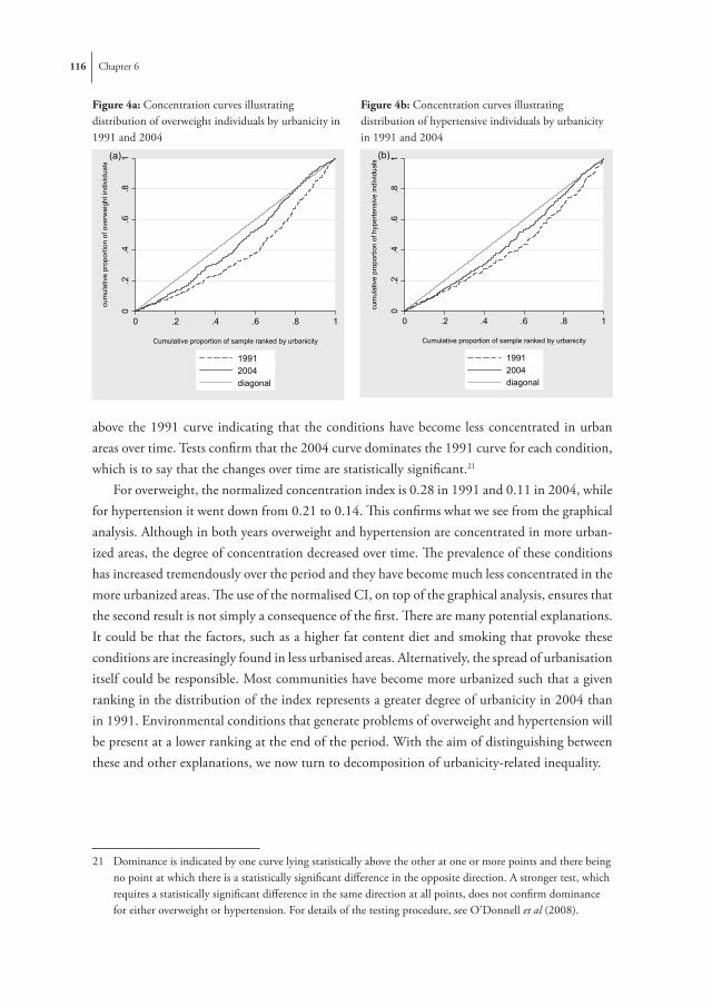
116 Chapter 6
above the 1991 curve indicating that the conditions have become less concentrated in urban areas over time. Tests confirm that the 2004 curve dominates the 1991 curve for each condition, which is to say that the changes over time are statistically significant.21
For overweight, the normalized concentration index is 0.28 in 1991 and 0.11 in 2004, while for hypertension it went down from 0.21 to 0.14. This confirms what we see from the graphical analysis. Although in both years overweight and hypertension are concentrated in more urban-ized areas, the degree of concentration decreased over time. The prevalence of these conditions has increased tremendously over the period and they have become much less concentrated in the more urbanized areas. The use of the normalised CI, on top of the graphical analysis, ensures that the second result is not simply a consequence of the first. There are many potential explanations. It could be that the factors, such as a higher fat content diet and smoking that provoke these conditions are increasingly found in less urbanised areas. Alternatively, the spread of urbanisation itself could be responsible. Most communities have become more urbanized such that a given ranking in the distribution of the index represents a greater degree of urbanicity in 2004 than in 1991. Environmental conditions that generate problems of overweight and hypertension will be present at a lower ranking at the end of the period. With the aim of distinguishing between these and other explanations, we now turn to decomposition of urbanicity-related inequality.
21 Dominance is indicated by one curve lying statistically above the other at one or more points and there being no point at which there is a statistically significant difference in the opposite direction. A stronger test, which requires a statistically significant difference in the same direction at all points, does not confirm dominance for either overweight or hypertension. For details of the testing procedure, see O’Donnell et al (2008).
Figure 4a: Concentration curves illustrating distribution of overweight individuals by urbanicity in 1991 and 2004
Figure 4b: Concentration curves illustrating distribution of hypertensive individuals by urbanicity in 1991 and 2004
0.2
.4.6
.8ke
rnel
den
sity
urb
anic
ity in
dex
-2 0 2
kernel density for urban kernel density for rural
Figure 3: Kernel density estimates of the urbanicity index for urban/rural communities as defined in the CHNS. Note: Based upon data pooled across all waves (1991, 1993, 1997, 2000 and 2004).
0.2
.4.6
.81
cum
ulat
ive
prop
ortio
n of
ove
rwei
ght i
ndiv
idua
ls
0 .2 .4 .6 .8 1
Cumulative proportion of sample ranked by urbanicity
19912004diagonal
(a)
Figure 4a: Concentration curves illustrating distribution of overweight individuals by urbanicity in 1991 and 2004
0.2
.4.6
.81
cum
ulat
ive
prop
ortio
n of
hyp
erte
nsiv
e in
divi
dual
s
0 .2 .4 .6 .8 1
Cumulative proportion of sample ranked by urbanicity
19912004diagonal
(b)
Figure 4b: Concentration curves illustrating distribution of hypertensive individuals by urbanicity in 1991 and 2004
-20%
-10%
0%
10%
20%
30%
40%
50%
60%
urban
icity
index
incom
e
educ
ation
occu
patio
n
phys
ical a
ctivit
y
fatint
ake
alcoh
ol & sm
oking
demogra
phics
provin
ceerr
or
19912004
Figure 5a: Percentage contributions of categories of variables to urbanicity-related inequality in overweight in 1991 and 2004

Urbanization and the spread of diseases of affluence in China 117
Explanation of urbanicity-related inequalities in 1991
Concentration indices of the covariates, which indicate how these are distributed across the urbanicity index, are presented in the first column of Table 6. Note that a positive concentration index means that the variable is disproportionately concentrated in more urbanized areas and a negative index indicates the opposite.
The signs of the concentration indices appear quite intuitive for most variables. Income and education are higher in more urbanized areas. Farming is clearly more prevalent in the more rural areas, whereas all other occupations are concentrated in urban communities22. Among the lifestyle variables, physical activity is distributed pro-rural and alcohol and fat intake are more concentrated in urban areas. We find that older people are more concentrated in urban areas, which might be related to the higher life expectancy in urban areas (Liu et al 1999). Henan province is relatively rural, whereas Liaoning and Shandong are significantly more urbanized, as is also visible from Figure 1.
In the second column of Table 6 we present the coefficients from the linear probability model with overweight as the dependent variable. Elasticities are given in the third column. Since the urbanicity index has no intuitive unit of measurement, it is not entered into the regression directly. Instead, we include dummy variables to indicate whether the individual’s community is among the middle third or the top third most urbanized communities across the whole 1991-2004 period. After controlling for all covariates, individuals living in the top third most urbanized communities are eight percentage points more likely to be overweight that those in the bottom third, a difference that is strongly statistically significant.23
For the remaining covariates our findings generally correspond to those found in the litera-ture. While income is positively associated with the probability of being overweight, education is protective against being overweight. All occupations are associated with lower overweight than the professional category; being a farmer is most protective. Not working and being a skilled worker has no significant effect. Among the lifestyle variables we find that physical activity is protective against overweight while fat intake is significantly associated with a higher risk of being overweight. There is a negative association between smoking and overweight. Young people (below 30 years of age) have the lowest risk of being overweight, females have a higher
22 The proportion of farmers decreases steadily across quintiles of the urbanicity index, but even in the upper quintile 2% of individuals are involved in farming.
23 To get insight into which of the components of the index are mostly driving this association, we have run some models explaining the probability of being overweight by the urbanicity index dummy variables with and without control for sets of community covariates. The effect of the urbanicity index is quite robust to controlling for indicators of services, transportation and the socioeconomic context, but falls substantially (by a half to two-thirds) after controlling for land use (farmland and workagri). This suggests that these community characteristics are responsible for a large part of the correlation between the urbanicity index and being overweight. The same is true for hypertension. Results are available upon request from the authors.

118 Chapter 6 Urbanization and the spread of diseases of affluence in China 119
Tabl
e 6:
Dec
ompo
sitio
n of
urb
anic
ity re
late
d in
equa
litie
s in
obes
ity a
nd h
yper
tens
ion
in 1
991.
O
verw
eigh
tH
yper
tens
ion
cate
gory
inde
pend
ent v
aria
ble
conc
entr
atio
n in
dex
(1)
coeffi
cien
t (2)
elas
ticity
(3)
prop
ortio
nate
co
ntrib
utio
n (4
)co
effici
ent (
5)el
astic
ity (6
)pr
opor
tiona
te
cont
ribut
ion
(7)
C
I xkβ k
(βk*
Xk/H
)
β k(β
k*X
k/H)
urba
nici
tym
iddl
e th
ird0.
167*
**0.
009
0.02
00.
014
-0.0
03-0
.005
-0.0
05
top
third
0.72
6***
0.07
9***
0.16
30.
489*
**0.
026*
0.05
10.
198*
*
soci
oeco
nom
ic
statu
s
log
inco
me
0.03
5***
0.01
4***
0.74
80.
110*
**0.
013*
**0.
656
0.12
5***
prim
ary
educ
atio
n-0
.135
***
0.01
00.
016
-0.0
09-0
.022
*-0
.033
0.02
4*
seco
ndar
y ed
ucat
ion
0.04
6***
-0.0
18-0
.040
-0.0
07-0
.045
***
-0.0
92-0
.022
***
high
er e
duca
tion
0.31
7***
-0.0
53**
*-0
.065
-0.0
85**
*-0
.057
***
-0.0
66-0
.111
not w
orki
ng0.
291*
**0.
002
0.00
20.
003
0.07
6***
0.10
80.
169*
**
farm
er-0
.398
***
-0.0
71**
*-0
.244
0.40
3***
0.01
40.
047
-0.1
00
skill
ed w
orke
r0.
371*
**-0
.024
-0.0
13-0
.019
-0.0
12-0
.006
-0.0
12
non-
skill
ed w
orke
r0.
318*
**-0
.064
***
-0.0
41-0
.054
***
-0.0
04-0
.003
-0.0
04
othe
r wor
k0.
356*
**-0
.052
***
-0.0
30-0
.045
**-0
.011
-0.0
06-0
.012
lifes
tyle
phys
ical
act
ivity
-0.3
52**
*-0
.012
-0.0
460.
067
-0.0
44**
*-0
.153
0.28
9***
log
fat i
ntak
e0.
015*
**0.
023*
**0.
695
0.04
3***
0.00
30.
086
0.00
7
smok
er-0
.012
-0.0
50**
*-0
.121
0.00
6-0
.036
***
-0.0
810.
005
alco
hol
0.03
8**
0.01
50.
011
0.00
20.
078*
**0.
052
0.01
0*

118 Chapter 6 Urbanization and the spread of diseases of affluence in China 119
O
verw
eigh
tH
yper
tens
ion
dem
ogra
phic
s
Mal
e 30
-44
-0.0
32*
0.05
7***
0.06
6-0
.009
*0.
051*
**0.
056
-0.0
10
Mal
e 45
-64
0.02
7*0.
079*
**0.
074
0.00
80.
186*
**0.
161
0.02
3
Mal
e 65
+0.
248*
**0.
056*
*0.
015
0.01
5**
0.36
9***
0.09
10.
121*
**
Fem
ale
16-2
9-0
.042
***
-0.0
14-0
.020
0.00
3-0
.059
***
-0.0
770.
017*
**
Fem
ale
30-4
4-0
.046
***
0.08
2***
0.11
3-0
.021
***
-0.0
07-0
.010
0.00
2
Fem
ale
45-6
40.
059*
**0.
134*
**0.
136
0.03
3***
0.12
1***
0.11
40.
036*
**
Fem
ale
65+
0.18
8***
0.08
8***
0.02
70.
021*
**0.
316*
**0.
089
0.08
9***
mar
ried
0.00
20.
035*
**0.
199
0.00
20.
001
0.00
80.
000
prov
ince
Jiang
su-0
.013
-0.0
08-0
.008
0.00
0-0
.014
-0.0
130.
001
Shan
dong
0.21
6***
0.10
0***
0.10
00.
090*
**0.
082*
**0.
077
0.08
9***
Hen
an-0
.253
***
0.09
8***
0.07
7-0
.081
***
0.05
7***
0.04
2-0
.057
***
Hub
ei0.
064*
*0.
012
0.01
20.
003
0.06
9***
0.06
50.
022*
Hun
an-0
.020
-0.0
41**
*-0
.037
0.00
30.
031*
*0.
026
-0.0
03
Gua
ngxi
-0.0
07-0
.067
***
-0.0
520.
001
-0.0
16-0
.012
0.00
0
Liao
ning
0.11
7***
0.04
7***
0.04
30.
021*
*0.
147*
**0.
125
0.07
8***
er
ror
-0.0
02
-0
.009
0.02
8
O
verw
eigh
tH
yper
tens
ion
Nor
mal
ized
conc
entr
atio
n in
dex
bein
g de
com
pose
d0.
280
0.21
0
Not
es: D
ecom
posit
ion
as in
equ
atio
n (3
). C
oeffi
cien
ts fro
m li
near
pro
babi
lity
mod
el. P
ropo
rtio
nate
con
trib
utio
n is
the
cont
ribut
ion
of th
e co
varia
te to
urb
anic
ity-r
elat
ed
ineq
ualit
y in
ove
rwei
ght/h
yper
tens
ion
rela
tive
to th
e co
ncen
trat
ion
inde
x fo
r the
resp
ectiv
e ris
k fa
ctor
. Gui
zhou
is th
e re
fere
nce
prov
ince
. *
indi
cate
s sig
nific
ance
at 1
0%, *
* at
5%
, ***
at 1
% (b
ased
upo
n bo
otstr
appe
d sta
ndar
d er
rors
).

120 Chapter 6
Figure 5a: Percentage contributions of categories of variables to urbanicity-related inequality in overweight in 1991 and 2004
Figure 5a: Percentage contributions of categories of variables to urbanicity-related inequality in overweight in 1991 and 2004
-20%
-10%
0%
10%
20%
30%
40%
50%
60%ur
bani
city
inde
x
inco
me
e
duca
tion
occu
patio
n
phys
ical
act
ivity
fat i
ntak
eal
coho
l & s
mok
ing
dem
ogra
phic
s
prov
ince
erro
r
% c
ontri
butio
ns
1991 2004
Notes: Contribution of each category is the sum of the cont ributions given in Tabl es 6 & 7 ove r the variables in the category. C ategories are defined as fo llows: urbancity in dex (m iddle th ird, top third ), income (log income), education (primary, secondary, higher education), occupation (not working, farmer, skilled worker, non-skilled worker, other worker), fat intake (log fat in take), alcohol & sm oking (alcohol, smoker), demographics (Male 30-44, Female 65+, … married), province (Jiangsu,…Liaoning).
Figure 5b: Percentage contributions of categories of variables to urbanicity-related inequality in hypertension in 1991 and 2004
Figure 5b: Percen tage contrib utions of categories of v ariables to u rbanicity-related in equality in hypertension in 1991 and 2004
-20%
-10%
0%
10%
20%
30%
40%
50%
60%
70%
urba
nici
ty in
dex
inco
me
e
duca
tion
occu
patio
n
phys
ical
act
ivity
fat i
ntak
eal
coho
l & s
mok
ing
dem
ogra
phic
s
prov
ince
erro
r
% c
ontri
butio
ns
1991 2004
Notes: as for Figure 5a. Notes: Contribution of each category is the sum of the contributions given in Tables 6 & 7 over the variables in the category. Categories are defined as follows: urbancity index (middle third, top third), income (log income), education (primary, secondary, higher education), occupation (not working, farmer, skilled worker, non-skilled worker, other worker), fat intake (log fat intake), alcohol & smoking (alcohol, smoker), demographics (Male 30-44, Female 65+, … married), province (Jiangsu,…Liaoning).

Urbanization and the spread of diseases of affluence in China 121
risk than men, and middle-aged women (between 45 and 65 years of age) are the most likely to be overweight. In addition, married individuals are more likely to be overweight. The province effects confirm the north-south gradient discussed before, with individuals living in Shandong, Henan and Liaoning more likely to be overweight than those from Guizhou, who, in turn, are more likely to be overweight than those living in Guangxi and Hunan.
In the fourth column of Table 6 we present the proportionate contribution of each variable to the concentration index for overweight, which is computed from the decomposition pre-sented in equation (3). The percentage contributions of groups of related variables are presented in Figure 5a. One half of the inequality in overweight related to urbanicity is driven by the direct effect of the urbanicity index, which captures the impact of community characteristics on the propensity to be overweight that does not operate through the socio-demographic characteris-tics of the population, or its behavior. The next largest contribution comes from the occupation variables (29%), and particularly from being involved in farming (40%). That is, two-fifths of the inequality in the prevalence of overweight across more and less urbanized communities is explained by differences in engagement in farming given the strong negative association of this occupation with overweight. Higher incomes in more urbanized areas explain 11% of the inequality in overweight, a contribution that is cancelled out entirely by the higher education of more urbanized populations. Differences in the fat content of the diet explain 4% of the greater concentration of overweight in more urbanized areas. About the same proportion of the inequality (5%) is attributable to the fact that the urban populations are older. The province dummies jointly only contribute an insignificant 4%, suggesting that macro level factors are relatively unimportant in explaining differences in overweight by urbanicity. The contribution of the error term is negligible (-1%), indicating that our set of observed covariates does a good job in explaining urbanicity-related inequalities.
The regression results for hypertension, which are presented in the fifth and sixth columns of Table 6, generally confirm the patterns observed for overweight. Hence, we only discuss those that differ. Hypertension increases with age and is more prevalent among males, which can be seen, for example, from the significant negative coefficient for females aged 16-29 indicating a lower prevalence relative to the reference category of males of the same age. Fat intake is not significantly associated with hypertension, and smoking is negatively associated. While cigarette smoking is a well-known risk factor for hypertension, other studies for China have also reported counter-intuitive results (He et al 1995; Hou, 2008), which may derive from the strong posi-tive correlation between smoking and socioeconomics that are not sufficiently captured by the education and income variables (Pan 2004). Occupation is not significantly associated with hypertension, although the unemployed face a higher risk.
In the seventh column of Table 6 we present the results of the decomposition of urbanicity-related inequality in hypertension, which appear to be related to several factors. A summary of these results is given in Figure 5b. The direct effect of the urbanicity index accounts for about a fifth (19%) of the inequality. Income differences explain 13% of the concentration of

122 Chapter 6
hypertension in more urbanized communities. As was the case for overweight, the education advantage in urbanized areas helps suppress their greater risk of hypertension, reducing the inequality by 11%. Differences in physical activity contribute most (29%) to the inequality. Rural populations engage more in physical activity, which helps reduce the risk of hypertension. The contribution of the demographics is almost equally large (28%) and results from the fact that hypertension increases with age and older people are more concentrated in urban areas. The provincial dummy variables make a larger contribution (13%) than is the case for overweight, mostly deriving from Shandong and Liaoning being both relatively urbanized and suffering from higher hypertension rates. Again, the contribution of the error term is quite small and insignificant (3%).
Explanation of urbanicity-related inequalities in 2004 and their changes from 1991
Keep in mind that the urban concentration of both overweight and hypertension decreased between 1991 and 2004 and that, as is made clear by the decomposition (3), this may be because the determinants of each disease risk factor are becoming less concentrated by urbanicity, and/or because the risk factor has become less correlated with those determinants. Changes in the urban concentration of determinants of overweight (hypertension) are observed by comparing the concentration indices in the first (fifth) column of Table 7 with the corresponding values in Table 6. Similarly, comparison of the coefficients in the second (sixth) columns of the two tables reveals changes in the effects of determinants on the risk factors. The net effect of changes in the distribution and the effect of a determinant is seen by comparing the contributions in the fourth (seventh) columns of the tables.
Urbanicity, represented by whether a community is in the middle or in the top third of the distribution across the whole 1991-2004 period, itself has become more equally distributed, indicating that the most rural communities have been catching up in terms of infrastructure and services. The association between (log) income and urbanicity has apparently declined by 2004, but one needs to be careful in comparing concentration indices for log incomes since the transformation will reduce the spread at the top of the distribution. Smoking has become significantly more prevalent in rural areas (He et al 1995; Yang et al 1999). There have been shifts in the distribution of demographics, with younger people being more concentrated in urban areas in 2004. This might be a consequence of age-selective rural-urban migration, with younger people moving away from rural areas (Wu 1994). Further, there have been changes in the relative urbanicity of the provinces. Relative to the other provinces, Hunan and Guangxi have become more urbanized while the opposite happened in Hubei, Shandong and Liaoning (Figure 1).
The associations between the covariates and overweight have remained quite stable over time. The urbanicity index is still significant and positively associated with overweight. The

Urbanization and the spread of diseases of affluence in China 123
effect of education, particularly its highest level, has decreased in magnitude and is no longer significant in 2004, which may be an indication that unhealthy eating habits are spreading to the better educated groups. Heavy physical activity in 2004 has a significant negative effect on overweight. By 2004, Jiangsu and Hubei have reached higher overweight rates than Guizhou, whereas the difference between Guizhou and Hunan is no longer significant.
The decomposition results of urbanicity-related inequality in overweight in 2004 (fourth column in Table 7 and Figure 4b) confirm the importance of the urbanicity index itself, the contribution of which declines only marginally. After this direct effect, overweight continues to be lower in less urbanized areas because of the higher engagement in farming. The contribution of higher incomes in more urbanized areas remains stable and, in 2004, is only partially offset by the more highly educated population since the magnitude of the education contribution falls by almost half and does not remain significant. Less engagement in physical activity by urban populations becomes much more important in explaining their greater propensity to be overweight; differences in this characteristic explaining more than a quarter of urbanicity-related inequality in 2004. The contribution of the demographics has disappeared, due to the lower age of the urban population in 2004 as compared to 1991. Although the province dummy variables are still jointly insignificant, the point estimates suggest that differences at the province level decrease urbanicity-related inequality in overweight. This is mainly due to the fact that the more southern provinces (Guangxi and Hunan) have become relatively more urbanized without experiencing a higher increase in overweight rates than the more northern and central regions (Liaoning, Shandong and Hubei) which have become relatively less urbanized compared to other regions, while maintaining their higher overweight rates.
From the fifth column of Table 7 it is apparent that quite a few of the associations between the covariates and hypertension have disappeared by 2004. Income, alcohol intake and the occupational variables are no longer significantly associated with hypertension. One can only speculate about the causes of these changes. As average incomes rise, it may be that lifestyles that provoke hypertension have filtered further down the income distribution. It is not immediately obvious why the correlation with alcohol has been reduced. Given the alcohol variable is a dummy for whether the person drinks daily, it could be that the proportion of heavy drinkers in this group has fallen. The urbanicity index itself, on the other hand, has become much more associated with hypertension, which suggests that community level factors have increased in importance relative to individual characteristics as determinants of hypertension.
Due to the stronger association between hypertension and the urbanicity index, the direct contribution of the latter to urbanicity-related inequality increases threefold to 62% in 2004 (Table 7, column seven and Figure 5b). On the other hand, the contributions of demographics, income, alcohol, province effects, and physical activity all decrease. The drop in the contribution of the province effects results from the same processes as discussed before.

124 Chapter 6
Tabl
e 7:
Dec
ompo
sitio
n of
urb
anic
ity re
late
d in
equa
litie
s in
obes
ity a
nd h
yper
tens
ion
in 2
004.
O
verw
eigh
tH
yper
tens
ion
cate
gory
inde
pend
ent v
aria
ble
conc
entr
atio
n in
dex
(1)
coeffi
cien
t (2)
elas
ticity
(3)
prop
ortio
nate
co
ntrib
utio
n (4
)co
effici
ent (
5)el
astic
ity (6
)pr
opor
tiona
te
cont
ribut
ion
(7)
C
I xkβ k
(βk*
Xk/H
)β k
(βk*
Xk/H
)
urba
nici
tym
iddl
e th
ird-0
.276
***
0.01
20.
017
-0.0
500.
021
0.03
5-0
.095
top
third
0.55
1***
0.04
9***
0.08
30.
495*
**0.
066*
**0.
131
0.71
4***
soci
oeco
nom
ic
statu
s
log
inco
me
0.02
4***
0.01
4**
0.43
80.
114*
*0.
003
0.10
30.
025
prim
ary
educ
atio
n-0
.145
***
0.00
10.
000
-0.0
01-0
.012
0-0
.012
0.01
7
seco
ndar
y ed
ucat
ion
-0.0
22*
-0.0
12-0
.014
0.00
3-0
.037
**-0
.052
0.01
1
high
er e
duca
tion
0.28
5***
-0.0
21-0
.019
-0.0
59-0
.047
**-0
.050
-0.1
42**
not w
orki
ng0.
196*
**-0
.037
-0.0
54-0
.113
0.01
20.
021
0.04
1
farm
er-0
.441
***
-0.0
80**
*-0
.092
0.43
9***
-0.0
19-0
.026
0.11
1
skill
ed w
orke
r0.
243*
**-0
.060
-0.0
09-0
.023
0.01
80.
003
0.00
7
non-
skill
ed w
orke
r-0
.001
-0.0
67**
-0.0
140.
000
-0.0
07-0
.002
0.00
0
othe
r wor
k0.
256*
**-0
.046
*-0
.018
-0.0
49*
-0.0
05-0
.002
-0.0
06
lifes
tyle
phys
ical
act
ivity
-0.4
08**
*-0
.045
***
-0.0
610.
267*
*-0
.026
*-0
.041
0.16
6*
log
fat i
ntak
e0.
015*
**0.
027*
*0.
426
0.06
7**
-0.0
03-0
.065
-0.0
09
smok
er-0
.034
***
-0.0
62**
*-0
.065
0.02
4***
-0.0
40**
-0.0
490.
016*
alco
hol
-0.0
19-0
.021
-0.0
090.
002
0.02
30.
011
-0.0
02

Urbanization and the spread of diseases of affluence in China 125
dem
ogra
phic
s
Mal
e 30
-44
-0.0
100.
092*
**0.
045
-0.0
050.
060*
**0.
035
-0.0
03
Mal
e 45
-64
-0.0
34**
*0.
109*
**0.
082
-0.0
30*
0.22
9***
0.20
0-0
.067
*
Mal
e 65
+0.
101*
**0.
057*
*0.
014
0.01
60.
355*
**0.
106
0.10
5***
Fem
ale
16-2
90.
049*
-0.0
74**
*-0
.019
-0.0
10-0
.084
***
-0.0
26-0
.012
Fem
ale
30-4
4-0
.051
***
0.04
2*0.
025
-0.0
14-0
.034
*-0
.024
0.01
2
Fem
ale
45-6
4-0
.018
0.13
7***
0.11
4-0
.022
0.11
4***
0.11
1-0
.019
Fem
ale
65+
0.13
3***
0.08
0**
0.02
30.
033*
*0.
351*
**0.
116
0.15
3***
mar
ried
-0.0
11**
*0.
070*
**0.
213
-0.0
27**
0.01
10.
038
-0.0
04
prov
ince
Jiang
su0.
006
0.09
2***
0.05
60.
003
0.07
8***
0.05
50.
003
Shan
dong
0.07
5***
0.20
9***
0.10
20.
082*
**0.
089*
**0.
051
0.03
8**
Hen
an-0
.080
***
0.17
3***
0.07
5-0
.065
**0.
094*
**0.
048
-0.0
38*
Hub
ei-0
.194
***
0.04
9**
0.02
0-0
.042
**0.
098*
**0.
047
-0.0
91**
*
Hun
an0.
157*
**-0
.004
-0.0
01-0
.002
0.01
00.
004
0.00
6
Gua
ngxi
0.06
2**
-0.0
64**
*-0
.030
-0.0
20-0
.001
0.00
0-0
.000
Liao
ning
0.01
20.
171*
**0.
078
0.01
00.
146*
**0.
078
0.00
9
er
ror
0.00
5
-0.0
22
0.
053
O
verw
eigh
tH
yper
tens
ion
Nor
mal
ized
conc
entr
atio
n in
dex
bein
g de
com
pose
d0.
110
0.14
0
Not
es: a
s for
Tab
le 6

126 Chapter 6
Discussion
This paper has quantified, tracked and explained the distribution of two important risk factors for chronic disease—overweight and hypertension—across Chinese communities at various stages of the urbanization process over the period 1991-2004. Both in 1991 and in 2004, over-weight and hypertension were more prevalent in the more urbanized areas. However, while the prevalence rates of these conditions have almost doubled over the period 1991-2004, inequali-ties across areas at different stages of urbanization have narrowed.
We used decomposition analysis to identify the factors that are driving these inequalities and their narrowing trend. More than half of the urbanicity-related inequality in overweight is at-tributable to the direct effect of the community level characteristics that underlie the urbanicity index. This suggests that environmental factors are important determinants of overweight and that the higher prevalence in more urbanized areas is not merely an artifact of the characteristics of the population located there. For hypertension, the relative contribution of community level characteristics to the explanation of urbanicity-related inequality trebles from 20% in 1991 to 62% in 2004. Environmental factors are becoming increasingly important determinants of the spread of this health condition. These could relate to changes in community diet and eating habits associated with the move away from agriculture and the rising number of restaurants. Improved transportation facilities, and increased use of motorized transport, contribute to more sedentary life styles and thereby to overweight and hypertension (Monda, Gordon-Larsen et al 2007). Urbanization also brings about changes in the social context of communities, which have been shown to increase stress and blood pressure (Niakara et al 2007).
Within the set of individual level factors, it is especially differences in engagement in physi-cal activity and farming, both protective against overweight and hypertension and concentrated in more rural areas, that contribute to the lower prevalence of these health problems in less urbanized areas. This is in line with previous work which has argued that moving away from agriculture based employment to more sedentary work plays an important role in the rise of overweight in China (Monda, Gordon-Larsen et al 2007). While both income and education are typically higher in urban areas, the former is associated with higher, and the latter with lower, overweight and hypertension. For this reason, the distribution of income increases and that of education decreases urbanicity-related inequalities in these conditions.
To maintain the sample size, we did not use information on population density (as opposed to population size) in computation of the urbanicity index (note 7). It turns out that the relative contributions of factors to urbanicity-related inequality change little when density is used. For inequality in overweight, the direct contribution of the urbanicity index, which one would expect to be most responsive to inclusion of population density, falls only marginally from 50%
Urbanization and the spread of diseases of affluence in China 127
to 47% in 1991 and slightly more from 44% to 33% in 2004. For hypertension, the direct contribution changes from 19% to 12% in 1991 and from 62% to 64% in 2004.24
Three main factors appear to be associated with the declining urbanicity-related inequalities in both overweight and hypertension from 1991 to 2004. First, urban areas have obtained a higher concentration of young people, who are less prone to being overweight or hypertensive. This is likely to result from the age-selective rural to urban migration and actually masks the urban concentration of these risk factors. Secondly, we find that those provinces that urbanized faster during the period 1991-2004 (Hunan and Guangxi) did not experience higher increases in overweight/hypertension rates than provinces like Shandong, Liaoning and Hubei that were already relatively urbanized in 1991. This suggests that the more recent urbanization trends are less accompanied by rising overweight and hypertension, which might also be due to a shorter exposure time to the increased urbanicity. A third trend is related to the spread of urbanization itself. Our urbanicity index has become more equally distributed over time, which indicates that relatively more rural communities are catching up in terms of transport infrastructure, economic activity and community services. In other words, much of China is becoming more urbanized to some degree and with this the environmental conditions that encourage the spread of health problems such as overweight and hypertension are being established in relatively less urbanized communities.
An apparent fall in absolute differences in urbanicity seems to contrast with the huge media coverage given to the urban-rural divide in China (e.g. UN 2008) and must be interpreted subject to three caveats. First, our estimates of urbanicity-related inequalities derived from the CHNS do not necessarily reflect inequality trends for China as a whole. Second, our composite index might have difficulty discriminating between the urbanized and the most urbanized communities, including those located in megacities, as they are characterized not only by the community variables in our index, but also by other aspects such as modernization, techno-logical progress, foreign investment etc. A third limitation of our study, also related to the representativeness of the CHNS panel, is that migrants that arrive in urban areas after the first wave will not be captured in the survey. Since there are estimated to be as many as 130 million migrant workers in China (National Bureau of Statistics China 2006), this is potentially important. Without knowledge of their rates of overweight and hypertension relative to the permanent rural and urban populations, one cannot speculate on the direction and magnitude of the bias their omission creates.
Despite the aforementioned caveats, it is by no means the case that our finding of a decreas-ing urban concentration of overweight and hypertension is attributable to the coverage of the CHNS and the properties of the urbanicity index. Decreasing urbanicity-related inequalities in risk factors for non-communicable diseases is quite consistent with increasing income inequality.
24 Detailed results of the decomposition with population density included in the factor analysis are available from the authors on request.

128 Chapter 6
While urban-rural income disparities are growing in China, economic development and rising average incomes produce environmental conditions that raise susceptibility to cardiovascular disease throughout the country. According to the China Human Development Report (UNDP 2005) infant mortality rates in rural China are more than double those of urban areas (34 versus 14 per 100 live births) and the difference in life expectancy between the urban and rural populations increased from 3.5 years in 1990 to 5.7 years in 2000. Therefore, what is happening to the urbanicity-related inequalities in risk factors for chronic diseases is not necessarily true for other health outcomes.
As this paper is not identifying causal effects of urbanization on overweight/hypertension, we should be careful in drawing direct policy recommendations. Our findings do, however, reveal important issues that deserve the attention of policy makers. The first issue relates to the importance of community level characteristics in explaining urbanicity-related inequalities in risk factors for cardiovascular disease. In the case of hypertension, the contribution of com-munity level determinants is increasing. Although many of the changes in community facilities and infrastructure, such as better transport facilities, are desirable, they may nonetheless have negative consequences for population health. The finding that community characteristics con-tribute substantially to inequalities in overweight/hypertension – even after controlling for the individual level determinants – suggests that there is scope for community-level interventions to curb increasing overweight/hypertension rates. This proposition is supported by recent work by Currie et al (2009) that shows that proximity to fast food restaurants has a causal impact on overweight rates among school children in the United States. Public health measures need to focus not only on campaigns to influence individual health behavior, but also on environmental factors that condition behavior through opportunities for, and constraints on, healthy living.
A second policy issue arising from our analysis relates to the decline in urbanicity-related inequality in overweight/hypertension due to the fact that the urbanicity itself is becoming more evenly spread as China develops. That is, the environmental conditions that raise susceptibility to these risk factors are materializing more widely throughout China. This suggests that public health measures and specialized health services should not be confined to the large population centers, but need to reach the periphery which, itself, is becoming more urbanized.
In sum, this paper confirms that chronic health conditions associated with modernization and affluence, such as overweight and hypertension, are becoming a pressing problem in China, and, more originally, it reveals that the phenomenon is no longer an exclusively urban one. As development and urbanization are spreading within the Eastern and Central provinces of China, so are the diseases of affluence. Over the past 25 years, China has made extraordinary progress in reducing the number of people living in poverty, helping to combat its associated health problems. However, new chronic diseases are threatening some of the health gains from this progress. Given that universal health insurance coverage is still a long way off and consequently there is heavy reliance on direct payments for medical care (Liu et al 1999), onset of a chronic illness represents a huge economic burden for millions of Chinese households. An important

Urbanization and the spread of diseases of affluence in China 129
challenge lies in accompanying continued growth, development and urbanization with early preventive warnings that changing lifestyles will pose new health threats that ultimately carry their own economic costs.

7The health penalty of China’s rapid urbanization
Rapid urbanization could have positive and negative health effects, such that the net impact on population health is not obvious. It is, however, highly pertinent to the human welfare consequences of development. This paper uses
community and individual level longitudinal data from the China Health and Nutrition Survey to estimate the net health impact of China’s unprecedented urbanization. We construct an index of urbanicity from a broad set of community characteristics and define urbanization in terms of movements across the distribution of this index. We use difference-in-differences estimators to identify the treatment effect of urbanization on the self-assessed health of individuals. The results reveal important, and robust, negative causal effects of urbanization on health. Urbanization increases the probability of report-ing fair or poor health by 5 to 15 percentage points, with a greater degree of urbanization having larger health effects. While people in more urbanized areas are, on average, in better health than their rural counterparts, the process of urbanization is damaging to health. Our measure of self-assessed health is highly correlated with subsequent mortal-ity and the causal harmful effect of urbanization on health is confirmed using more objective (but also more specific) health indicators, such as physical impairments, disease symptoms and hypertension.

132 Chapter 7
Introduction
Urbanization and economic development are intimately related (Williamson 1988). There is no better example of this than China in recent decades, where a remarkable rate of economic growth has been accompanied by a process of urbanization that is unprecedented in human history, both in scale and in speed. The proportion of the Chinese population living in urban areas increased from only 20% in 1980, to 27% in 1990, and reached 43% in 2005 (National Bureau of Statistics China 2006; World Bank 2006). By the middle of this century, the country’s urbanization rate has been forecast to reach 75% (Yusuf & Saich 2008). In the space of just a few decades, China will complete the urbanization process that lasted hundreds of years in the West. The non-economic consequences of such rapid urbanization, including those for health, as well as more obviously for the environment, will determine the true welfare effects of develop-ment and the extent to which it is sustainable. The consequences for population health are not obvious. On the one hand, urban living offers improved access to modern medicine (particularly in China) and gains in income that can be invested in health. On the other, the health of city dwellers is threatened by air pollution, more sedentary and possibly more stressful work, social detachment, and Western, high-fat diets. This paper uses panel data from China covering the period 1991-2004 to estimate the net health impact of urbanization.
On average, health outcomes are found to be better in urban parts of the developing world (Van de Poel et al 2007; Zimmer et al 2007). This apparent urban health advantage contrasts with the historical evidence of urban populations suffering poorer health in Western Europe prior to and during its period of industrialization (Rosen 1958; Woods 1985, 2003). The most likely explanation for this difference in the urban-rural health disparity over time and space is the marked decline in the prevalence of infectious diseases, in low-income as well as high-income countries (Riley 2005), prompted, in large part, by public health measures built on the germ theory of disease (Preston 1975, 1980; Cutler & Miller 2005) and the introduction of effective medicines, antibiotics and vaccinations (Davis 1956; Cutler et al 2006; Soares 2007). In the past, the opportunities for material gain offered by cities had to be weighed against the dangers of infection. Today, while cities of the developing world continue to pose risks to health, the immediate threat to life through infection has receded. However, the overcrowding and pollution that accompany urbanization, particularly on the scale and speed with which it has occurred in China, may impose an urban health penalty. During the last decades, China’s environment has deteriorated significantly as rapid urbanization and industrialization generate enormous volumes of air and water pollutants (World Bank 1997; Wang & Smith 2000; Brajer & Mead 2003).1 As other developing countries, most notably India, China relies very heavily on coal as a source of energy, with the result that levels of airborne pollution in Chinese cities
1 But the health effects of pollution from urbanization are not necessarily limited to urban areas. Rural areas rely more on unsafe water sources and are also affected by pollutants coming from urban areas (WHO 2001).

The health penalty of China’s rapid urbanization 133
are many times greater than those found in most US and European cities (Pandey et al 2006).2 A World Health Organization study has estimated that there are 300,000 premature deaths per year in Chinese cities attributable to outdoor air pollution (Cohen et al 2004).3
Urbanization brings social and economic changes that can raise risk factors associated with chronic disease. Urban populations of middle-income countries are experiencing a rapid nutri-tional transition towards Western-style diets, dominated by more processed foods and a high fat content (Popkin 2001; Popkin & Du 2003). Urbanization inevitably implies a shift in work patterns from physical, agricultural labor towards more sedentary occupations (Monda, Adair et al 2007). In China, it is claimed that these transitions have contributed to stark increases in the prevalence of obesity and hypertension (Liu et al 2004; Wang et al 2007; Weng et al 2007).
But urbanization clearly has positive, as well as negative, consequences for population health. Closer proximity to health care facilities, particularly hospitals, equipped with modern technology and staffed by highly trained doctors is an obvious advantage of living in towns and cities. In China, urban-rural differences in access to health care, and in health insurance cover, have been marked and widening in recent decades (Liu et al 1999). Access to schools and to health education initiatives confer a strong advantage on urban areas in the field of preventative health care. Urban populations can also use higher incomes to invest in health through health care, a nutritious diet or by reducing strenuous work effort (Moore et al 2003).
In this paper, we estimate the net effect of urbanization on health using longitudinal data from the China Health and Nutrition Survey (CHNS). Besides being a household panel, this survey also collects data on the characteristics of communities, making it possible to identify what happens to individuals’ health when the environment in which they live becomes more urbanized. This identification strategy avoids the selection biases that arise from comparisons between the health of urban and rural populations, or from monitoring the health of migrants, which is difficult or impossible in any case with most panel data.
A dichotomous urban-rural classification, most often done on the basis of population density, does not capture the variation in living and health conditions across areas at different stages of urbanization (McDade & Adair 2001; Vlahov & Galea 2002; Champion & Hugo 2004; Dahly & Adair 2007). In addition, there is a practical problem in that the categorization of an area as ‘urban’ or ‘rural’ is often fixed over waves of a longitudinal survey, as it is in the
2 Across Chinese cities each with a population of at least 100,000, the weighted average of estimated airborne particulate matter concentrations (PM10) is 87 μg/m3 (Pandey et al 2006). The equivalent figure for US cities is 25. It is 13 in Sweden, 15 in France, 19 in the UK and 22 in Germany. The WHO study (Cohen et al 2004) predictions of premature deaths due to outdoor air pollution are based on these estimates.
3 As pointed out in footnote 1, the health effects of pollution in rural areas should not be overlooked. The WHO study estimated that 420,000 deaths per year in all of China are caused by indoor air pollution created by the burning of solid fuels, which rural households rely on for 90% of their energy needs (Zhang & Smith 2007).

134 Chapter 7
CHNS, and so this categorization does not capture the urbanization taking place. In order to identify communities at various stages of the urbanization process, and to track changes over time in the degree of urbanicity within each community, we exploit the CHNS data on the characteristics of communities to construct an index of urbanicity, which depends, for example, on population size, the proportion of the workforce engaged in agriculture, proximity to health and educational facilities, and the presence of paved roads, shops, restaurants, etc. This index has been shown to outperform the simple urban-rural classification that comes with the CHNS in detecting different degrees of urbanicity, measuring changes in urbanicity over time and being less prone to misclassification bias (Van de Poel et al 2009). We define urbanization in terms of movement of a community up the distribution of this urbanicity index. We adopt a treatment effects framework and define treatment as movement from the bottom to the top half of the distribution of the index. To investigate whether the health impact varies with the degree of urbanization, we also define ordinal treatments in terms of movements up tertiles of the distribution and by standard deviation increases in the index. We use difference-in-differences estimators made robust to unobserved individual heterogeneity by exploiting the panel nature of the data (Blundell & Costa Dias 2000; Wooldridge 2002).
The main health outcome used in the paper is self-assessed health (SAH), reported on a four-point scale from excellent to poor. This general measure of adult health has repeatedly been shown to be highly predictive of mortality, even conditional on physiological measures of health (Idler & Benyamini 1997). We show that SAH predicts mortality in the CHNS and demonstrate that it is highly correlated with more specific health outcomes such as obesity, hypertension, physical impairments and symptoms of illness. We also estimate the impact of urbanization on these narrower, but more objective, measures of health status.
To our knowledge, this is the first paper to estimate the causal effect of urbanization on health from longitudinal data on both individuals and communities. These data allow us to identify the effect of urbanization by comparing the health transitions of individuals living in areas that experience rapid transformations to an urban environment with those living in areas that remain rural. We find important, and robust, negative effects of urbanization on health. Urbanization increases the probability of reporting fair or poor health by 5 to 15 percentage points, with a greater degree of urbanization having larger health effects. While people in more urbanized areas are, on average, in better health than their rural counterparts, the process of ur-banization is damaging to health. Urbanization raises the probability of suffering from physical impairments, disease symptoms and hypertension, but there is no significant impact on obesity or under-nutrition.
In the remainder, we first present the CHNS data, and explain construction of the urbanic-ity index. This is followed by an explanation of our identification strategy, estimation methods and the various definitions of urbanization used. In the fourth section, we first present the main results for the impact of urbanization on SAH, and then check their robustness, before examin-

The health penalty of China’s rapid urbanization 135
ing the impact on other health outcomes. The concluding section provides an interpretation of the implications of the study and acknowledges its limitations.
Data
Sample
We use the China Health and Nutrition Survey (CHNS) panel data from 1991, 1993, 1997, 2000 and 20044. The CHNS is a large scale longitudinal survey conducted in 9 provinces in China: Liaoning, Shandong, Jiangsu, Henan, Heilongjiang, Hubei, Hunan, Guangxi and Gui-zhou. Although the CHNS is not representative of all China, these provinces vary substantially in terms of geography, urbanization and economic development. While the CHNS provinces span some of the relatively more urbanized regions of China, Beijing and Shanghai, the two largest megacities in China, are not covered. Urbanization rates vary considerably within each province. There have been some changes in the composition of the CHNS sample across time. Liaoning province was added in 1997 when Heilongjiang Province was unable to participate. Heilongjiang returned to the study in 2000 (and Liaoning remained as well). New households in original communities were added to replace households no longer participating in the study in 1997 and in 2000. In 1997, new communities in original provinces were added to replace sites no longer participating in the survey.5
The CHNS collects information on a wide range of individual, household and community characteristics. A community, which is the primary sampling unit (PSU), is a government-designated administrative district. The community interview is held with the community head for questions related to public facilities and infrastructure, and with community health workers for questions related to health care provision. In total, there are about 200 communities in each wave (see Chapter 6 – Table 3); an average of about 20 communities in each province. On average, there are about 15 households and a little less than 50 individuals interviewed within each community.
There are a total of 47418 person-wave observations across the five waves of the survey. After dropping observations with missing information on any of the individual or household level variables used in the regression analysis, or missing community characteristics used in construction of the urbanicity index, we are left with 31333 person-wave observations. 19% of respondents are only interviewed once in the survey, 25% twice, 26% three times, 20% four
4 In the 1989 survey, health and nutritional data were only collected from preschoolers and adults aged 20-45.
5 More information on this survey can be found at the Carolina Population Center CHNS website: http://www.cpc.unc.edu/projects/china.

136 Chapter 7
times and 9% are interviewed in all waves. The panel dynamics and attrition rates are shown in Table 1. There is quite a high attrition rate, which is partly because Heilongjiang province was not interviewed in 1997. Individuals reporting poor health are more likely to drop out of the sample between the last two waves. We test for attrition bias in the analysis below.
Measurement of urbanization
In order to track the increasing urbanization that is taking place in communities across the sur-vey waves, we construct an urbanicity index using factor analysis on a broad set of characteristics from the CHNS community level data pooled across all survey waves (Van de Poel et al 2009). The urbanicity index captures information on population size, land use in the community, transportation facilities, economic activity and public services (see Chapter 6 – Table 3). We have checked the validity of the urbanicity index in various dimensions and found that the fac-tor loading of the community variables have intuitive signs; the time trend in the index indeed reveals increasing urbanization; the index correlates with a subjective classification of communi-ties as urban, suburb, town or rural, that is available within the CHNS and with income (Van de Poel et al 2009).6 Although the urbanicity index is highly correlated with the administratively defined urban-rural classification available in the CHNS, it provides considerable additional information by displaying substantial variation within each category of the dichotomy.
Since the index is estimated from data on all communities in all waves, an increase in its value for a single community across time represents that community becoming more urbanized, in terms of reduced reliance on agriculture and increased availability of community infrastructure, services, etc, relative to the average over all communities within the whole period from 1990 to 2004.7 If, within each wave, communities were homogeneous with respect to urbanicity, then the index would increase for all communities over time reflecting the general process of urbanization experienced commonly by all. Of course, in reality, communities differ greatly in their characteristics at each point in time and so changes in the index indicate not only the general process of urbanization but also the specific one experienced by a community relative to all others.
6 This subjective classification is not very useful for our purposes as there is not much variation across the survey waves. Van de Poel et al (2009) found that cities and towns have the highest average urbanicity index, followed by suburban and rural areas. This means that suburban areas do not come second on the continuum from city to rural.
7 Similar, a decrease in the index points to deterioration in community infrastructure, meaning ‘de-urbanization’ has taken place. However, small changes in the index can also reflect reporting errors in the community survey. We return to this issue at the end of the Results section.

The health penalty of China’s rapid urbanization 137
Tabl
e 1:
Attr
ition
in C
HN
S.
at
triti
onhe
alth
rela
ted
attr
ition
wav
e#
indi
vidu
als
drop
out
sre
join
ers
surv
ival
rate
raw
dro
p ou
t rat
e (%
)
net d
rop
out r
ate
(%)
raw
dro
p ou
t ra
te e
xcel
lent
at
t-1
raw
dro
p ou
t ra
te g
ood
at
t-1
raw
dro
p ou
t rat
e fa
ir at
t-1
raw
dro
p ou
t ra
te p
oor a
t t-1
late
r-jo
iner
s
1991
6685
1993
3489
3196
00.
520.
480.
480.
520.
460.
470.
5639
50
1997
2482
1961
954
0.37
0.56
0.29
0.48
0.57
0.57
0.58
5201
2000
2050
1309
877
0.31
0.53
0.17
0.54
0.52
0.55
0.51
2350
2004
2559
658
1167
0.38
0.32
-0.2
50.
300.
310.
320.
4225
67
Not
es: Th
e su
rviv
al ra
te is
the
perc
enta
ge o
f orig
inal
sam
ple
mem
bers
rem
aini
ng a
t wav
e t.
The
drop
-out
rate
is th
e di
ffere
nce
in o
bser
vatio
ns b
etw
een
wav
es t−
1 an
d t r
elat
ive
to
the
num
ber o
f obs
erva
tions
at t
−1. Th
e ra
w d
rop-
out r
ate
excl
udes
rejo
iner
s, w
hile
the
net d
rop-
out r
ate
incl
udes
them
. Not
e th
at th
is ta
ble
only
con
sider
s the
se in
divi
dual
s pre
sent
in
the
1991
wav
e; la
te-jo
iner
s are
pre
sent
ed in
the
last
colu
mn.

138 Chapter 7
Since the index is constructed from factor analysis, it has no meaningful unit of measurement. We therefore identify the urbanization of a community through changes in its rank position in the (whole period) distribution of the index, conditioning on those that start off in the bottom part of the distribution. That is, we compare communities that move from the bottom to the top half of the distribution with those that remain in the bottom half. In 1991, 60% of the sample of communities were below the (all wave) median of the urbanicity index, while by 2004 61% of the sample was above the median. To investigate a dose-response effect, we also compare those that remain in the bottom third of the distribution with those that move from there to the middle and to the top third. The percentage of communities in the top (middle) third of the whole-period urbanicity distribution increased from 24% (30%) in the 1991 to 43% (35%) in 2004. To estimate the health effects of further urbanization in communities that are among the most urbanized even at the beginning of the panel, we also define treatment in terms of standard deviation increases in the index without conditioning on the initial degree of urbanicity.
Measurement of health
We use self-assessed health (SAH) as the principal measure of health. Respondents aged 18 years or over were asked to rate their health compared to that of people their own age on a four-point scale consisting of excellent, good, fair and poor. In the analysis, we mainly use a binary indicator of reporting fair or poor health (poorhealth), but in some specifications we exploit the informa-tion contained in the full ordinal scale.
SAH is a popular instrument for health status that is very widely used in research based on large scale household surveys. This is not just due to its availability, but because it provides a measure of general health status and numerous studies have demonstrated that it contains infor-mation on health over and above that which can be measured objectively by physiology-based instruments (Idler & Benyamini 1997). Two potential limitations of the measure are, first, that its very generality means that it cannot reveal the dimensions of health that are most affected by a treatment, such as urbanization, and, second, that any heterogeneity in the reporting of health that is correlated with the treatment will bias the estimated effect. In the present context, report-ing heterogeneity would affect our results if individuals living in communities that urbanize were to change their health expectations and therefore revise their SAH evaluation. To address both issues, we make use of the following more objective, but narrower, measures of health: mortality; obesity (Body Mass Index (BMI)>30); underweight (BMI<18.5); measured hypertension; re-ported physical impairments (goiter or angular stomatitis, loss of use of one or both arms or legs, blindness in one or both eyes); and, reported symptoms experienced in the four weeks preceding the survey (fever, headache, rash, diarrhea, joint pain, heart problems or others).
Table 2 shows the means of these more objective health indicators. Except for risk factors for chronic conditions, such as obesity and hypertension, most of the ill health indicators have a

The health penalty of China’s rapid urbanization 139
very low prevalence rate. Therefore, we create a binary variable that equals one if the respondent reported to suffer from at least one of the physical impairments. Also we use a binary variable to indicate whether the respondent reported any of the symptoms in the four weeks preceding the survey.
Table 3 confirms that SAH is correlated with each of the more objective measures of health. The first four columns show marginal effects from probit models explaining the probability of reporting fair or poor health. All of the more objective indicators of ill-health are significantly related with an increased probability of reporting fair or poor health, indicating that the latter binary measure captures at least some of the information contained in these more specific mea-sures. The last three columns of Table 3 show marginal effects on the probability of dying by
Table 2: Description and means (proportions) of ill health indicators.
Description of variables (1/0) Mean
BMI>30 0.025
BMI<18.5 0.079
diagnosed hypertension: average of three systolic blood pressure measurements (at time of survey) was≥140mm Hg and/or average diastolic blood pressure was ≥90mm Hg and/or respondent was taking medication to lower blood pressure 0.185
physical impairments:
goiter/angular stomatitis 0.010
loss of one arm or the use of 1 arm 0.002
loss of both arms or use of both arms 0.001
loss of one leg or the use of 1 leg 0.003
loss of both legs or use of both legs 0.001
blindness in one eye 0.002
blindness in both eyes 0.001
suffering from any of the above impairments 0.076
symptoms experienced in 4 weeks preceding the survey:
fever, sore throat, cough 0.044
headache, dizziness 0.037
rash, dermatitis 0.003
diarrhea, stomachache 0.020
joint pain, muscle pain 0.026
heart disease/chest pain 0.009
other symptoms 0.020
suffering from any of the above symptoms 0.106
whether respondent dies by subsequent wave 0.021
Observations 31333

140 Chapter 7
the subsequent wave. These results show that reporting fair or poor health at time t is predictive of mortality by the subsequent wave (column 5), increasing the baseline probability of dying by about one third, and that this predictive power remains after controlling for the set of more objective health indicators (column 6). This demonstrates that not only is the reporting poor or fair health strongly correlated with the other health indicators; but that it contains additional in-formation relevant to predicting mortality. The last column of Table 3 illustrates that the marginal effect of reporting fair or poor health on mortality is an average of a smaller effect of fair health on the probability of dying by the next wave (0.004) and a much larger impact of poor health (0.04).
Control covariates
To identify the health effect of urbanization, we control for a set of individual and household level characteristics including demographics (age, sex, marital status, household size), socio-economic status (education, income8) and household living conditions (availability of a flush
8 Household income is calculated by summing all market earnings across the household and then adding the total value of all other non-market goods and services produced within that household (see Liu et al 2008, Fig. 1). Total household income is then deflated using a year/province/urban-rural specific consumer price index that was developed for use with the CHNS, and divided by the (square root of the) total number of household members to obtain real average household income per capita (Liu et al 2008).
Table 3: Correlation between SAH and more objective health measures. Marginal effects from probit regression.
marginal effect on the probability of
reporting fair or poor healthmarginal effect on the probability
of dying by next wave
poorhealth (SAH=fair or poor)
0.007*** 0.005***
SAH=good 0.002
SAH=fair 0.004**
SAH=poor 0.037***
BMI>30 0.044** -0.002
BMI<18.5 0.090*** 0.007***
hypertension 0.051*** 0.005***
suffering from any impairments
0.069*** 0.005**
suffering from any ill-health symptoms
0.283*** 0.005***
Observations 29664 29707 31333 31001 31333 29598 31333
Notes: Models also include covariates as described in Table 4 and wave dummies. Standard errors are adjusted for clustering on individuals.* significant at 10%; ** significant at 5%; *** significant at 1%

The health penalty of China’s rapid urbanization 141
toilet, use of solid fuels within the dwelling, water from a water plant and the presence of excreta around the household dwelling). Although the latter living conditions can also be correlated with a community’s level of urbanization, we leave these variables out of the urbanicity index and include them separately in the models because they are not solely determined on the com-munity level, but also by households’ decisions. The exact definitions of all these variables are given in Table 4.
Table 4: Description of explanatory variables.
variable Description
demographics
age age (years)
age squared age squared
male whether respondent is male (1-0)
married whether respondent is married (1-0)
count number of household members
socioeconomic status
edno whether respondent has had no education (1-0)
edprim whether respondent’s highest education is primary education (1-0)
edmid whether respondent’s highest education is secondary education (1-0)
edhigh whether respondent’s highest education is higher education (1-0)
logincome logarithm of household income (in Chinese Yuan)
household living conditions
flush whether household has flush toilet (1-0)
excreta whether there is some or much excreata around the dwelling (1-0)
waterplant whether household has access to water that comes from a waterplant (1-0)
fuel whether household uses solid fuels within dwelling (1-0)
Notes: Underscored variables are used as reference category in regression models.
Item non-response is only substantial for the urbanicity index (24%) and household income (10%). The high proportion of missing information on the urbanicity index is due to the fact that it is constructed from a set of community variables, and so a missing value for any com-munity characteristic causes the index to be missing for all individuals in that community.9
Table 5 shows summary statistics of the individual and household level health determinants across all 5 waves of the CHNS. The trends illustrate the rising (average) incomes in China in the period 1991-2004. Also household living conditions (water, sanitation, heating) seem to have improved substantially. The distribution of the sample across the provinces has remained quite stable, with Heilongjang entering the survey only in 1997. The last rows of Table 5 clearly
9 Note that the community characteristics included in the urbanicity index have already been (partly) selected on the basis of their high response levels.

142 Chapter 7
Table 5: Means of covariates by wave.
Variable 1991 1993 1997 2000 2004
age 41.16 41.59 42.06 44.37 47.90
age squared 1936.06 1962.75 2020.35 2190.70 2529.20
male 0.47 0.48 0.50 0.48 0.48
married 0.78 0.78 0.75 0.80 0.83
size 3.98 3.98 4.14 3.44 3.24
edno 0.36 0.32 0.28 0.23 0.21
edprim 0.20 0.22 0.23 0.23 0.23
edmid 0.28 0.29 0.31 0.32 0.31
edhigh 0.16 0.17 0.18 0.21 0.25
log income 6.92 7.20 7.27 7.64 8.03
flush 0.18 0.24 0.29 0.33 0.44
excreta 0.22 0.21 0.15 0.10 0.09
waterplant 0.44 0.45 0.49 0.47 0.50
fuel 0.85 0.79 0.69 0.61 0.57
Liaoning 0.12 0.12 0.00 0.10 0.10
Heilongjang 0.00 0.00 0.08 0.09 0.12
Jiangsu 0.13 0.16 0.16 0.18 0.13
Shandong 0.13 0.10 0.10 0.08 0.11
Henan 0.11 0.08 0.18 0.09 0.12
Hubei 0.13 0.13 0.10 0.12 0.10
Hunan 0.12 0.13 0.05 0.07 0.08
Guangxi 0.10 0.13 0.14 0.10 0.12
Guizhou 0.17 0.16 0.18 0.15 0.13
urbanicity index -0.27 -0.14 -0.12 0.11 0.38
below (all-wave) median of urbanicity index (1/0) 0.57 0.51 0.54 0.49 0.38
above (all-wave) median of urbanicity index (1/0) 0.43 0.49 0.46 0.51 0.62
in lowest third of (all-wave) distribution of urbaniciy index (1/0) 0.44 0.39 0.37 0.27 0.20
in middle third of (all-wave) distribution of urbanicity index (1/0) 0.30 0.32 0.32 0.36 0.35
in upper third of (all-wave) distribution of urbanicity index (1/0) 0.26 0.29 0.31 0.37 0.45
Observations 6685 5298 6040 5339 7971

The health penalty of China’s rapid urbanization 143
illustrate the rapid urbanization taking place in China, with the urbanicity index rising from -0.27 in 1991 to 0.38 in 2004.
Identification strategy and estimation
As explained in the previous section, urbanization is defined in terms of movement of a com-munity up the distribution of the urbanicity index, either from the bottom to the top half, or from the bottom to higher tertiles, and by standard deviation increases in the index. We identify the health impact of such urbanization by using difference-in-differences (DID) methods to compare the changes in health of those living in communities that experience urbanization with those that do not.
Model and estimation
We begin by restricting attention to individuals living in communities that are not urbanized at the beginning of the survey period, defined as those in the bottom half, or bottom third, of the distribution of the urbanicity index. A DID estimator of the treatment effect of urbanization is then obtained from the following logit model applied to the binary measure of SAH (and each of the other health outcomes examined) (Wooldridge 2002; Blundell et al 2004; Puhani 2008; Böckerman & Ilmakunnas 2009):
147
treatment effect of urbanization is then obtained from the following logit model
applied to the binary measure of SAH (and each of the other health outcomes
examined) (Wooldridge 2002; Blundell et al 2004; Puhani 2008; Böckerman &
Ilmakunnas 2009):
*igt
*1 2 3 4 5
1 if y 0igt
igt t g gt igt ig igt
y
y x z
(1)
where i indexes individuals, g indexes treatment (urbanization) groups, defined at the
level of the community, and t indexes time. igty equals one if the individual reports to
have fair or poor health at time t . The model includes a full set of time dummies t ,
which capture trends in reported health that are common across all individuals, and a
set of treatment group dummies g , which capture time-invariant differences between
those individuals living in communities that at some time experience a defined degree
of urbanization and those that do not. The time varying group dummies, gtx , equal
one if the individual is exposed to a defined degree of urbanization at time t . Since
we restrict the sample to those in the bottom part of the distribution of the urbanicity
index at the beginning of the panel, these dummies are zero for all individuals at their
first observation. The estimate of the average treatment effect of urbanization on the
probability of experiencing fair or poor health is given by the marginal effect of these
dummies. Further, we control for individual covariates igtz (see Table 4) and a full set
of both community and province dummies ig .10
Although time-invariant differences between treatment and control
communities are taken into account, this DID estimator does not exploit the panel 10 In order to avoid the introduction of other indices to denote communities and provinces, we define
ig to be a set of dummies that for a given treatment group g, which indicates whether or not urbanization is ever experienced, varies across individuals according to the precise community and province in which they are located.
(1)
where i indexes individuals, g indexes treatment (urbanization) groups, defined at the level of the community, and t indexes time. yigt equals one if the individual reports to have fair or poor health at time t. The model includes a full set of time dummies λt, which capture trends in reported health that are common across all individuals, and a set of treatment group dummies αg, which capture time-invariant differences between those individuals living in communities that at some time experience a defined degree of urbanization and those that do not. The time varying group dummies, xgt, equal one if the individual is exposed to a defined degree of urbanization at time t. Since we restrict the sample to those in the bottom part of the distribution of the urbanicity index at the beginning of the panel, these dummies are zero for all individuals at their first observation. The estimate of the average treatment effect of urbanization on the probability of experiencing fair or poor health is given by the marginal effect of these dummies. Further, we

144 Chapter 7
control for individual covariates zigt (see Table 4) and a full set of both community and province dummies δig.
10
Although time-invariant differences between treatment and control communities are taken into account, this DID estimator does not exploit the panel nature of the data and so is poten-tially rendered inconsistent by any individual level unobserved heterogeneity that is correlated with any of the right-hand-side variables in (1). We deal with this by applying the conditional logit estimator to a model like (1), but including a fixed unobservable individual level effect and, consequently, no time invariant regressors. This comes at the cost of smaller sample size, as the fixed effects logit model only uses those observations for which there is variation in the dependent variable.
With a third estimator, we exploit more of the information in the ordinal SAH variable by taking the approach of Ferrer-i-Carbonell & Frijters (2004), who have shown that an ordered logit model with fixed effects can be estimated as a fixed effects logit model, where the ordered data are collapsed to binary data and the model allows individual-specific thresholds.11 This involves creating a binary health indicator (worsehealth) that equals one if the individual reports worse health at time t than the average he/she reports across all waves and then using this as the dependent variable in a fixed effects variant of (1) estimated by conditional logit (Böckerman & Ilmakunnas 2009). In the remainder of the paper, we will refer to this as the fixed effects ordinal logit.
Using Verbeek & Nijman’s (1992) test, we found some evidence of attrition bias in the simple logit model.12 However, once fixed effects are taken into account, attrition can only in-duce inconsistency when selection is related to the idiosyncratic errors. We tested this by adding the lagged selection indicator to the fixed effects logit model and the fixed effects ordered logit model (estimated on the total panel), and doing a t-test for the significance of the selection indi-cator (Jones et al 2006).13 The null of no effect was not rejected in both models (p-value=0.781 and 0.199 respectively), indicating that our fixed effects estimators are not biased by attrition, providing further reason for focusing on them.
10 In order to avoid the introduction of other indices to denote communities and provinces, we define δig to be a set of dummies that for a given treatment group g, which indicates whether or not urbanization is ever experienced, varies across individuals according to the precise community and province in which they are located.
11 We have also estimated ordered probit models on the ordinal SAH variable and these results confirmed the ones with the binary health indicator.
12 This involves testing the significance of a count variable of the number of waves that are observed for the individual in the model explaining poorhealth. Under the null hypothesis, the error is uncorrelated with attrition for all t, and so attrition in the previous time period should not be significant in the equation at time t.
13 Note that this method loses the first time period for all observations.

The health penalty of China’s rapid urbanization 145
Throughout, standard errors are corrected for clustering at the individual (and so any higher) level.
Definition of urbanization
In a first instance, we define the treatment of urbanization as a community moving from below the median (across all waves) of the urbanicity index to above it. We only use those individuals living in communities that fall below the median of the urbanicity index when they are first interviewed. It is important to emphasize that this median is defined on the sample of com-munities pooled across all waves; which means that in principle every community could start off below the median and end up above it. In reality, at each wave, some communities will have crossed the median, and other will not. In this setting, model (1) will consist of only one treatment group dummy αg, equal to one in every wave if the individual’s community ever rises above the median, and only one treatment dummy xgt, which is unity only in the periods when the individual’s community is above the median. It is possible that communities experience a drop in their urbanicity index, which could cause them to be above the median in one wave and fall below it in the next. We keep these observations in the sample, and hereby treat urbanization as potentially reversible. At the end of the Results section, we will return to this issue.
We can also use model (1), and its variants that take account of fixed effects, to investigate whether the health effects vary with the intensity of urbanization by defining treatment indica-tors that distinguish between smaller and larger movements up the distribution of the urbanicity index. We consider the sample of individuals whose communities start off in the lowest third of the urbanicity index and define two treatments: a move to the middle third of the urbanicity index by any subsequent wave and a move to the upper third of the index. This model has two time invariant group dummies in αg and two time varying group dummies in xgt, and the marginal effects of the latter are the estimated treatment effects of the two intensities of urbanization.14
Finally, in order to investigate the health effects of increased urbanization from any level, and not only from originally non-urban environments, we estimate the effects of varying mag-nitudes of increase in the urbanicity index from one wave to the next. We examine increases of i) 0.25-0.5 standard deviations (sd), ii) 0.5-1 sd, iii) 1-1.5 sd and iv) more than 1.5 sd between waves. Note that we are not restricting the starting level of urbanicity to any particular interval. The reference category is therefore communities that experience an increase in the urbanicity index smaller than 0.25 of a standard deviation (or a decrease). It should also be noted that
14 Note that the treatment effect of first moving from the lowest to the middle third and then to the upper third is the same as moving to the upper third directly. We could not relax this assumption, because there are too few communities that actually jump from the lowest to the upper third from one wave to another.

146 Chapter 7
with this definition, the treatment dummy is only switched on in the wave in which the change occurs. In subsequent periods it is turned off, unless an increase of the same magnitude is repeated. Therefore, the treatment effects estimated with this approach will reflect only the short term health impact of increased urbanization, unlike with the other approaches which identify the health effect that materializes over the whole period in which a community is exposed to a higher degree of urbanicity.
Results
Effects on self-assessed health
We first look at the health effect of a jump from below to above the median of the urbanicity index. After deleting those observations that start off in the upper half of the distribution, we are left with 17864 observations, of which 43% move to the upper half.
Table 6 shows marginal effects obtained from the logit, fixed effects logit and fixed effects ordinal logit estimators. Sample sizes in the fixed effects models are substantially smaller because they only use observations that show variation in the dependent variable.15
All three models indicate a positive and significant treatment effect, indicating that urban-ization increases the probability of reporting poorer health. The magnitude of the effect is about 5 to 6 percentage points, an increase of almost one-fifth in the baseline probability of reporting fair or poor health for those not originally living in urban environments. The estimates from the fixed effects logit (second column) indicate that urbanization raises the probability of reporting fair or poor health (6.5%) by slightly more than having excreta around the household dwelling (6%) or using solid fuels indoors (5%), and a little less than not obtaining water coming from a waterplant (10%) or not having a flush toilet (8%). Note that the treatment effect in the fifth column refers to the effect of urbanization on the ordinal SAH variable, and is therefore not directly comparable to the effects in the previous columns for the binary health variable. This marginal effect of 0.054 should be interpreted as the increase due to urbanization in the probability of an individual reporting worse health than he/she did on average across the panel.
The marginal effect of the treatment group dummy is negative and significant in the logit model (first column), indicating that those individuals that do experience urbanization are on average in better health than those who do not. This is consistent with the better average health outcomes that are usually found in more urban areas (Van de Poel et al 2007; Zimmer et al 2007). The combination of the positive effect of the time-varying treatment dummy and the negative effect of the time invariant treatment group dummy indicates that people living in areas
15 The model using worsehealth as dependent variable exploits more of the variation in SAH and therefore uses more observations.

The health penalty of China’s rapid urbanization 147
Table 6: Marginal effects of urbanization and covariates on self-assessed health.
logit fixed effects logit fixed effects ordinal logit
poorhealth1 poorhealth1 worsehealth2
marginal
effectstandard
errormarginal
effectstandard
errormarginal
effectstandard
error
treatment 0.0407*** 0.014 0.065*** 0.020 0.054*** 0.017
treatment group -0.371*** 0.091
log income -0.020*** 0.003 -0.018*** 0.007 -0.019*** 0.005
married 0.014 0.011 0.071** 0.029 -0.014 0.025
edprim -0.035*** 0.010 0.011 0.039 0.048 0.035
edmid -0.044*** 0.012 -0.056 0.058 -0.01 0.049
edhigh -0.052*** 0.014 -0.092 0.094 0.024 0.077
age 0.008*** 0.002
age squared 0.000 0.000
male -0.056*** 0.008
waterplant -0.073*** 0.013 -0.097** 0.024 -0.073 0.020
flush -0.059*** 0.014 -0.078** 0.028 -0.086*** 0.023
excreta 0.052*** 0.010 0.058** 0.015 0.049*** 0.013
fuel 0.05*** 0.012 0.045** 0.023 0.051*** 0.019
size -0.007** 0.003 0.000 0.006 0.000 0.005
1993 -0.030** 0.012 -0.005 0.018 0.015 0.015
1997 -0.01 0.013 0.065*** 0.018 0.087*** 0.016
2000 0.138*** 0.015 0.249*** 0.025 0.227*** 0.018
2004 0.150*** 0.015 0.292*** 0.029 0.26*** 0.020
Liaoning -0.199*** 0.047
Heilongjang -0.262*** 0.039
Jiangsu -0.346*** 0.036
Shandong -0.303*** 0.026
Henan -0.234*** 0.070
Hubei -0.255*** 0.058
Hunan -0.26*** 0.040
Guangxi 0.034 0.077
Observations 17864 8284 10994
Notes: treatment equals one if community is in the upper half of the urbanicity index at time t. treated equals one if community is ever in the upper half. All models include community dummies (δig). Standard errors are adjusted for clustering on individuals.1 poorhealthit=1 if SAHit=fair or poor, 0 otherwise; 2worsehealthit=1 if SAHit>meani(SAH), 0 otherwise* significant at 10%; ** significant at 5%; *** significant at 1%

148 Chapter 7
that eventually become urbanized are originally in better health than their counterparts living in areas that do not become urbanized, but the process of urbanization is itself harmful to health.
It is interesting that there appears to be an increasing trend in the probability to report poor health in China during the period 1991-2004. Model (1) imposes the restriction that urbanization has the same effect in every year, an assumption that may, to an extent, be justified by the fact that our treatment is defined in terms of crossing the median of the index computed from the data pooled across all waves. So, in terms of the index, moving from below to above the median in 1993 is not necessarily different from doing so in 2004. But, for a given value of the index, the degree and nature of urbanization may differ over time. To allow for this, we included interactions between the treatment variable and the wave dummies, but these were never found to be significant.
The estimates show the expected correlations of health with individual and household level determinants. Reporting fair or poor health is increasing with age, and decreasing with income and education. The education effect is not significant in the models including individual fixed effects, most likely due to its limited variation across time. Married individuals and females are more likely to report poor or fair health. As noted above, all of the household living conditions variables are significant in the expected directions.
By controlling for income and living conditions, we may have taken out any indirect effect that urbanization has on health through these factors. To investigate whether this is the case, we re-estimated the fixed effects logit model without these controls. As can be seen from the first column of Table 7, dropping income reduces the magnitude of the treatment effect of urbanization slightly (from 0.065 to 0.057), indicating there is a small, positive indirect effect from urbanization through income to health. Leaving the household living conditions variables out has no impact on the estimate (column 3). Finally, without control for income and living conditions (column 5), the estimated marginal effect of urbanization falls only marginally from 0.065 to 0.061. These results suggest there is a small indirect positive effect of urbanization on health operating through increasing household income, but not through household living conditions, which only very slightly offsets the direct negative effect.
Effects of varying intensities of urbanization
We now examine whether the health effect varies with the intensity of urbanization. 13409 individuals live in communities that start off in the lowest third of the distribution of the urbanicity index, 66% move to the middle third of the urbanicity index sometime in the period 1991-2004, and 12% to the upper third. Results are presented in Table 8 for the same three estimators (as in Table 6). Note that sample sizes are smaller as compared to Table 6, because the sample is restricted to those communities that start off in the lowest third (not lowest half ) of the urbanicity index distribution. The results indicate that the treatment effect of moving

The health penalty of China’s rapid urbanization 149
from the lowest to the middle third of the urbanicity index is small and insignificant. However, moving from the bottom to the upper third of the index significantly increases the probability of reporting fair or poor health by about 6 percentage points in the logit model and 8 points in the fixed effects logit, which represents an increase of about one third in the baseline probability. The marginal effect estimated from the fixed effects ordered logit model implies that moving from the lower to the upper third of the index raises the probability of individuals reporting worse health than their average across survey waves by 0.12.
Next, we look at the estimated health effects of standard deviation changes in the urbanicity index. Because we use changes, the first observation is lost for each individual. 19% of the sample experiences an increase in the urbanicity index of 0.25-0.5 standard deviations, 18% an increase of 0.5-1 sd, 6% an increase of 1-1.5 sd and 4% an increase of more than 1.5 sd.
Table 7: Marginal effects of urbanization and covariates on self-assessed health – sensitivity to control for household income and living conditions.
fixed effects logit
poorhealth1
marginal
effectstandard
errormarginal
effectstandard
errormarginal
effectstandard
error
treatment 0.057*** 0.017 0.065*** 0.020 0.061*** 0.018
log income -0.020*** 0.006
married 0.060** 0.025 0.068** 0.029 0.060** 0.026
edprim 0.006 0.034 0.012** 0.041 0.008 0.037
edmid -0.052 0.053 -0.060 0.058 -0.060 0.056
edhigh -0.086 0.089 -0.114 0.091 -0.113 0.093
waterplant -0.088*** 0.023
flush -0.07*** 0.026
excreta 0.05*** 0.013
fuel 0.040** 0.020
size 0.001 0.005
1993 -0.009 0.015 -0.006 0.018 -0.011 0.017
1997 0.049*** 0.015 0.043** 0.018 0.030* 0.016
2000 0.193*** 0.020 0.244*** 0.021 0.195*** 0.016
2004 0.226*** 0.023 0.278*** 0.023 0.220*** 0.018
observations 8184 8284 8284
Notes: treatment equals one if community is in the upper half of the urbanicity index at time t. 1 poorhealthit=1 if SAHit=fair or poor, 0 otherwise; * significant at 10%; ** significant at 5%; *** significant at 1%.

150 Chapter 7
Table 9 shows the treatment effects of these different magnitudes of urbanization.16 Individuals living in communities that undergo very small increases in urbanization (0.25-0.5 sd increase in the index) actually have a slightly reduced probability of reporting fair or poor health relative to those that experience no increase (or decrease) in urbanization. But larger increases in urbaniza-tion cause deterioration in reported health, with the probability to report fair/poor health rising by as much as 15 percentage points for those experiencing an increase of more than 1.5 standard deviations in the urbanicity index. It should be kept in mind that these are short run effects in the sense that they materialize in the period immediately following the increased urbanization. Note that the magnitude of the change in the index is – as would be expected – negatively correlated with its initial value. So, consistent with Table 8, these results indicate that it is individuals originally living in more rural settings that undergo the most rapid urbanization experience the greatest deterioration in health.
Effects on other health outcomes
To check whether the negative health effects of urbanization reported in the previous sub-sections are simply attributable to changes in health expectations that accompany urbanization and to obtain more insight into which aspects of health are most affected by increasing urbanization,
16 Estimates are presented only for the fixed effects models since the fact that individuals can belong to several treatment groups makes definition of the treatment group dummies rather complicated for the simple logit. In any case, the fixed effects estimators are preferred.
Table 8: Marginal effects of urbanization on self-assessed health – ordinal treatments.
logit fixed effects logit
fixed effects ordinal logit
poorhealth1 poorhealth1 worsehealth2
marginal
effectstandard
errormarginal
effectstandard
errormarginal
effectstandard
error
treatment (bottom to middle third urbanicity index)
0.012 0.012 0.02 0.018 0.004 0.015
treatment (bottom to top third urbanicity index)
0.056* 0.034 0.081* 0.044 0.116*** 0.037
treatment group (bottom to middle) -0.442*** 0.114
treatment group (bottom to top) -0.092 0.075
Observations 13409 6425 8505
Notes: All models include community dummies (δig) and covariates as in Table 6 . Standard errors are adjusted for clustering on individuals.1 poorhealthit=1 if SAHit=fair or poor, 0 otherwise; 2worsehealthit=1 if SAHit>meani(SAH), 0 otherwise* significant at 10%; ** significant at 5%; *** significant at 1%.

The health penalty of China’s rapid urbanization 151
we now turn to estimates of the impact of urbanization on a set of more objective and specific health outcomes. Treatment of urbanization is defined as moving from the lower to the upper half of the distribution of the urbanicity index (as in Table 6). Logit and fixed effects logit estimates of the treatment effects are presented in Table 10. Sample sizes for the fixed effects models are much smaller, as these require some variation across time in the dependent variable, which is considerably smaller than in the SAH variables. The results reveal that urbanization increases the probability of suffering from hypertension (although the effect decreases and loses significance in the fixed effects logit), physical impairments and ill-health symptoms, but has no significant impact on under- and over-nutrition.17 This suggests that the health impact of urbanization does not operate through obesity, as a result of changes in diet and lifestyle, and there is only limited evidence of an effect through a cardiovascular disease risk factor, such as hypertension. Much more important are the effects on physical impairments and symptoms of illness and disease.18 From the fixed effects logit models, we estimate that urbanization almost doubles the baseline probability of suffering from physical impairments, and increases the base-line probability of suffering from ill-health symptoms by more than half. While the impact on symptoms may, in part, be due to changes in reporting behavior, this is unlikely to be true for physical impairments, which refer to losses of (use of ) arms, legs and sight, suggesting that the effect of urbanization on SAH is not solely reflecting a change in individuals’ health expectations
17 Estimating a fixed effects model on mortality did not prove useful, because of the small proportion of people dying and the fact that individuals drop out of the sample once they die.
18 We also tried excluding goiter/angular stomatitis from the list of physical impairments, as this is quite a different condition than the loss of (use of ) arms, legs and eyesight. This did not significantly change the treatment effect of urbanization. Goiter/angular stomatitis has been related to iodine deficiency, but also other factors such as contamination of water have been shown to play an important role (Kotwal et al 2006).
Table 9 Marginal effects of urbanization on self-assessed health.
fixed effects logit fixed effects ordinal logit
poorhealth1 worsehealth2
SD increase in the urbanicity index
marginal effect standard error marginal effect standard error
0.25-0.5 -0.034** 0.016 -0.029** 0.014
0.5-1 0.041** 0.017 0.023 0.015
1-1.5 0.034 0.026 0.020 0.023
>1.5 0.152*** 0.031 0.132*** 0.027
Observations 7806 10411
Notes: All models include community dummies (δig), and covariates as in Table 6. Standard errors are adjusted for clustering on individuals.1 poorhealthit=1 if SAHit=fair or poor, 0 otherwise; 2worsehealthit=1 if SAHit>meani(SAH), 0 otherwise* significant at 10%; ** significant at 5%; *** significant at 1%

152 Chapter 7
as their environment becomes more urbanized. Urbanization is also associated with an increased probability of dying, although the effect is not significant, which is perhaps not surprising given the low incidence of death.
Sensitivity to making urbanization irreversible
The urbanicity index is constructed using factor analysis on a broad set of community char-acteristics. Changes in the index therefore reflect actual increases or decreases in the presence or availability of community facilities and infrastructure. The strong increasing trend of the urbanicity index across the CHNS survey waves reflects the huge urbanization taking place in China. However, for some communities the index decreases from one wave to the next. These decreases are generally quite small and much less frequent than the increases in the index, and ―in the context of China’s urbanization― are more likely to reflect reporting errors in the recording of community characteristics rather than actual ‘de-urbanization’. To test whether our results are influenced by these potential errors, we replicated the analysis excluding these negative-change observations. In the case of the first definition of urbanization, i.e. crossing the median of the index, we excluded observations from communities that had returned to the
Table 10: Marginal effects of urbanization on probability of experiencing different health outcomes.
logit fixed effects logit
dependent variablemarginal effect of
urbanizationstandard
errormarginal effect of
urbanizationstandard
error
hypertension 0.026*** 0.008 0.017 0.026
observations 16734 3858
BMI>30 0.003 0.003 0.078 0.093
observations 16708 427
BMI<18.5 0.006 0.007 -0.041 0.040
observations 16708 1617
any physical impairments 0.017*** 0.006 0.095** 0.037
observations 17864 2974
any ill-health symptoms 0.009 0.006 0.061* 0.031
observations 17864 3817
dying by next wave 0.002 0.002
observations 17864
Notes:treatment equals one if community is in the upper half of the urbanicity index at time t; treated equals one if community is ever in the upper half. All models include community dummies (δig) and covariates as in Table 6. Standard errors are adjusted for clustering on individuals. Urbanization is defined as crossing the median of the urbanicity index (similar as in Table 6).* significant at 10%; ** significant at 5%; *** significant at 1%
The health penalty of China’s rapid urbanization 153
lower half of the index distribution, after having moved to the upper half in the previous wave (3% of the sample). With this restriction, the treatment of urbanization becomes irreversible, in the sense that once communities move to the upper half of the distribution they remain there. The treatment effects of urbanization on SAH based on this definition of ‘irreversible treatment’ and the restricted sample are presented in the Appendix – Table A1. The treatment effect remains positive and is significant for all but the fixed effects ordinal logit. Using the fixed effects logit, the estimated impact of urbanization on the probability of reporting fair or poor health falls from 0.065 with reversible treatment and the full sample to 0.053 with irreversible treatment and the restricted sample.
Conclusion
Urbanization is an important component of economic development. Indeed, it is difficult to imagine development occurring without a process of urbanization. The health consequences of urbanization not only represent a potentially important effect of development on human welfare, but may also act as a constraint on its sustainability. This paper investigates the net health effect of the tremendous urbanization taking place in China.
To identify communities at various stages of the urbanization process, and to track urbaniza-tion over time, we derive an urbanicity index from a broad set of community characteristics available in the CHNS. This, in combination with individual level panel data provides a rich source of variation from which to identify the health impact of urbanization. The results reveal substantial and significant negative effects of urbanization on health, with the probability of reporting poor or fair health increasing by 5 to 6.5 percentage points, an increase of almost one fifth in the baseline probability, when communities rise from the bottom to the top half of the distribution of urbanicity. This is comparable to the effects of household level living conditions such as excreta surrounding the household dwelling, use of solid fuels indoors, absence of a flush toilet and not obtaining water from a water plant. We find a small offsetting indirect effect of urbanization on health through income, but no indirect effects through household living conditions.
Larger degrees of urbanization have stronger health effects. Moving from the lowest to the top third of the distribution of urbanicity increases the probability of reporting fair or poor health by 6 to 8 percentage points, an increase of about a third in the baseline probability. An increase of more than 1.5 standard deviations in the urbanicity index is predicted to have severe and immediate adverse health effects, increasing the probability of reporting fair/poor health by 0.15. Our results confirm that people in urban areas are on average in better health than those in more rural areas, but the process of urbanization causes negative health effects.
While our panel estimators are robust to any time-invariant heterogeneity across individuals in the way they report their health, we cannot rule out the possibility that our results reflect

154 Chapter 7
across time variation in the reporting of health in response to the experience of urbanization. For example, people who experience urbanization, and are awakened to the potential of medical treatment for example, might raise their health expectations and therefore become more likely to report fair or poor health, given the same objective health. Deaton (2007) has found that, conditional on national income, recent economic growth makes people unhappier. If this phenomenon is present, our estimates reflect not only changes in objective medical conditions that respond to urbanization, but also the health consequences of the dissatisfaction individuals may derive from a changing environment. This is still a meaningful and relevant finding with respect to evaluation of the development process. But our results do not appear to derive only from an impact of urbanization on health expectations. Our SAH variable is a good predictor of mortality and correlates well with other more objective health outcomes such as hypertension, obesity, under nutrition, physical impairments and ill-health symptoms. The power of SAH to predict mortality remains after controlling for these more objective outcomes, indicating that it provides additional health information. Moreover, urbanization has a significant positive impact on the probability of suffering hypertension, physical impairments and symptoms of illness and disease. Moving from the bottom to top half of the distribution of urbanicity almost doubled the baseline probability of suffering from physical impairments and increased the probability of reporting any symptoms by about half.
In sum, we find that the Chinese are paying a health penalty for the tremendous urbaniza-tion they are experiencing, with larger urbanization causing worse health effects. This is a new and rather unexpected finding, as one typically associates urban populations with better health. Indeed, our analysis also found better average health in more urban areas. But given our finding that urbanization comes with negative net health consequences, it is questionable whether this urban health advantage will be sustained. To our knowledge, the net causal health effect of urbanization has gone unstudied, most likely because data were not available to measure changes in urbanization. Application of a composite index of urbanicity to panel data has allowed us to define various concepts of urbanization. The limitation of using such an index to identify the health effects of urbanization is that it is difficult to pinpoint which specific aspects of urban life have positive consequences for population health, and which are harmful to health. On the positive side, the closer proximity to health care, health insurance, health education, and economic opportunities are likely to benefit health (Liu et al 1999). But on the other hand, rapid and uncontrolled urbanization is also associated with pollution, overcrowding, social isolation, changes in dietary and physical activity patterns, and inadequate service capacity for providing drinking water, sanitation and waste disposal, which will penalize population health (Popkin 2001; WHO 2001; Moore et al 2003). Our analysis suggests that currently in China these negative aspects dominate the positive ones. Given the importance of cities in national and global economies, and the inevitability of increasing urbanization in China, it is of utmost importance to turn this effect around and foster sustainable and healthy cities.

The health penalty of China’s rapid urbanization 155
Appendix
Table A1: Marginal effects of urbanization on self-assessed health with irreversible definition of treatment.
logit fixed effects logit
fixed effects ordered logit
poorhealth* poorhealth* worsehealth**
marginal
effectstandard
errormarginal
effectstandard
errormarginal
effectstandard
error
treatment 0.039** 0.015 0.053** 0.021 0.026 0.019
treatment group -0.312*** 0.091
Observations 17401 7966 10531
Notes: treatment equals one if community is in the upper half of the urbanicity index at time t; treated equals one if community is ever in the upper half. Observations dropped from sample if living in community that experiences a move from above to below the median of the urbanicity index. All models include community dummies (δig). Standard errors are adjusted for clustering on individuals. 1 poorhealthit=1 if SAHit=fair or poor, 0 otherwise; 2worsehealthit=1 if SAHit>meani(SAH), 0 otherwise* significant at 10%; ** significant at 5%; *** significant at 1%


8Conclusion and policy recommendations

158 Chapter 8
This thesis sheds some light on the complex inter linkages between health and inequality in a developing world that is rapidly urbanizing. From an empirical perspective, the links between health, inequality and urbanization are not straightforward to study as there is no unambiguous definition of either of these concepts. Although the literature on measuring health, and health inequality is quite advanced (see e.g. Mackenbach & Kunst 1998; Gwatkin 2001; O’Donnell et al 2008), much less is known on how one should best measure urbanization and its health effects. Chapters 4 and 5 confirmed that urban-rural health disparities correlate highly with urban-rural differences in socioeconomic status, but they also revealed heterogeneity in popula-tion characteristics within rural, and especially within urban areas. Also, it appeared that the simple urban-rural dichotomy is an oversimplification which cannot adequately distinguish the different living and health conditions experienced in areas at different stages of urbanization. Therefore, in Chapters 6 and 7, the thesis moved away from this dichotomy and developed a continuous measure of urbanicity. This urbanicity index turned out to substantially outperform the urban-rural dichotomy by detecting different degrees of urbanicity, measuring changes in urbanicity over time and being free from misclassification bias. In Chapter 6 this index was used to quantify and track urbanicity related inequalities in obesity and hypertension in China. Prevalence rates of these disease risk factors have increased substantially over the last decade, but at the same time urbanicity related inequalities have narrowed. Finally, Chapter 7 of this thesis has investigated what actually happens to people’s health when they are exposed to increasing urbanization in China. This analysis demonstrated that, while people in more urban locations are in better health, the actual process of urbanization causes a net health penalty.
In the remainder, we discuss in more detail the research findings and policy implications of each of the Chapters in this thesis.
Socioeconomic inequalities in health
Chapter 2 and Chapter 3 investigated socioeconomic inequalities in child malnutrition in the developing world. Chapter 2 quantified socioeconomic inequalities in child stunting and wasting in a large set of developing countries using an adjusted concentration index. Almost everywhere in the developing world poor children suffer disproportionally more from malnu-trition than their richer counterparts. However, there appeared no relation between average malnutrition rates and socioeconomic inequality in malnutrition. This suggests that reducing the overall rate of malnutrition does not automatically lead to a reduction of these inequalities. Therefore policies should take into account the entire distribution of childhood malnutrition across socioeconomic groups, instead of focusing only on population averages as currently is the case in large scale development programs such as the Millennium Development Goals (UN 2006). The distribution of malnutrition across socioeconomic groups was found to take several forms ranging from mass deprivation, to queuing and exclusion, each of which imply

Conclusion and policy recommendations 159
different policies to reduce these inequalities. In the case of exclusion, programs targeted at specific population groups, i.e. the poorest, are urgently needed to achieve pro-equity outcomes while in other instances, such as mass deprivation, broad strengthening of the whole system or a combination of the two approaches is required.
Chapter 3 takes a closer look at which factors lie behind these socioeconomic inequalities in childhood stunting in Ghana. The decomposition framework proposed by Wagstaff, van Doorslaer et al (2003) allows decomposition of socioeconomic inequalities in malnutrition into inequalities in the determinants of malnutrition. It is important to note that the most important determinants of malnutrition are not necessarily also important in explaining socioeconomic inequalities and vice versa. Of course, for a variable to contribute to socioeconomic inequalities in malnutrition, it needs to be related to malnutrition, but on top of that it needs to be un-equally distributed across income groups. The results illustrated that, although bio-demographic variables such as a risky birth interval, size at birth, duration of breastfeeding and the sex of the child are quite strongly associated with a child’s nutritional status, they do not contribute to socioeconomic inequality in malnutrition because of their relatively equal distribution across socioeconomic groups. This comes back to the point made earlier: if policy makers are really concerned about reducing socioeconomic inequalities in health, they should take into account how ill health is distributed across socioeconomic groups, and which factors are driving this distribution.
The results in Chapter 3 illustrated that the high socioeconomic inequalities in childhood malnutrition in Ghana are -apart from wealth itself- mainly associated with regional char-acteristics and use of health care services. Wealth was responsible for about one third of the socioeconomic inequality in malnutrition, which means that poorer children were more likely to be malnourished, mainly because of their poverty. The large regional contributions, even after controlling for other factors such as household wealth and education, bring forward the issue of geographical targeting. Although geographic targeting of policies can lead to an under coverage of the truly needy and also result in significant leakage to non-needy populations, it is usually much easier to target geographical units than it is to target socioeconomic population groups. Clearly, the efficiency gains of allocating resources to certain regions within countries depend on the homogeneity of the population within these regions.
In most developing countries, populations in urban areas tend to be richer than those in rural areas. With this, also average health indicators are better in most urban areas. Even if these regional inequalities could be explained by differences in population characteristics, targeting health resources on the basis of rural-urban location would still be efficient if there were homo-geneity in these characteristics within rural and urban sectors. But the greater is within sector population heterogeneity, the stronger is the argument for allocating resources in relation to characteristics besides rural-urban location. Chapters 4 to 6 investigated these urban-rural and urbanicity related health inequalities and their underlying factors.

160 Chapter 8
Urban-rural and urbanicity related inequalities in health
As a first step, in Chapter 4, urban-rural disparities in child stunting and mortality across a set of 47 developing countries were quantified. Indeed, these results confirmed that urban children are on average healthier than their rural counterparts. The median rural-urban relative risk ratio is 1.4 for both stunting and child mortality but rural-urban disparities in the two indicators are not strongly correlated across countries and regions in the developing world. Most of the variation in the magnitude, and the explanation, of rural-urban disparities in child mortality is within and not across regions. The magnitude of the rural-urban gap in child health outcomes reflects, to a large extent, differences in wealth. In a few cases, stunting and mortality rates are actually higher in urban areas after controlling for wealth. This suggests that conditional upon socioeconomic status, the rural environment is healthier than the urban one in these countries, possibly because of pollution and overcrowding. The analysis also confirmed that socioeconomic inequalities in child health are larger within urban than within rural areas.
Given that average stunting and under-five mortality rates are higher in rural areas and that, on average, around three-quarters of the stunting/mortality occurs in those areas there is a strong efficiency case for giving priority to rural based programs. However, the analysis in Chapter 4 revealed the large within urban heterogeneity. This implies that policies that only target the rural populations will overlook the urban poor who are not better (and in some countries even worse) off than their rural counterparts. Given that the poor urban population is growing at considerable rates in the developing world (UN HABITAT 2001), the need for policies targeting these urban poor is becoming increasingly high.
Another option to reduce health inequalities would then be to target policies at poor communi-ties within urban (and/or rural) areas. The efficiency of this targeting strategy again depends on whether communities are relatively homogenous in population characteristics, or at least in those characteristics that are relevant for people’s health status. So far, we have tried to attribute health disparities to differences in household characteristics, not taking into account community level characteristics such as the availability of health facilities, and transport infrastructure. The analysis in Chapter 4 did show that in most of the countries studied, the urban-rural disparities in child health are to a large extent attributable to differences in household wealth. However, in more than a third of the countries studied, the urban-rural gap remained significant after controlling for wealth and other household characteristics. This could mean that community characteristics also play a role in explaining the gap. Chapter 5 studied the relative roles of community and household characteristics in explaining urban-rural disparities in child survival in a set of six Central and West sub-Saharan African countries. This involved developing a decomposition method that allowed explanation of the urban-rural gap in infant mortality by household and community characteristics, both observed and unobserved. It is important to take account of household and community level unobserved heterogeneity, as it is likely

Conclusion and policy recommendations 161
that there are important household and community factors that affect infant mortality but are not measured in the data. Examples include biological and genetic factors, cross-infection rates and health related behavior at the household level; and cultures and customs, geography, climate, and the quantity and quality of infrastructure at the community level. The results of this decomposition demonstrated that the rural-urban gap in infant mortality is explained by differences in the distributions of factors that determine mortality and not by differences in the effects of those determinants between rural and urban locations. Rural-urban differences in household level determinants, which explain two-thirds of the gap, are much more important than those in community level determinants. Among the household characteristics, it was found that housing conditions and access to utilities play a particular strong role. This suggests that policies aiming to reduce the excess rural infant mortality need to operate not only through investments in community infrastructure and health programs but also by targeting the mate-rial needs of disadvantaged households within rural communities. Conditions such as limited electricity and water supply contribute greatly to the rural-urban gap and derive both from a lack of community level infrastructure and from the inability of some households to exploit the infrastructure when it is available. In this respect, policy needs to operate at both the community and household levels to correct such deficiencies.
The analysis in this thesis has taught us that the urban-rural dichotomy is too broad to be useful in the targeting of policies. The disadvantageous average health outcomes in rural areas are mostly due to the worse household living conditions. But at the same time, there are urban slum areas in which households are exposed to the same, or even worse, conditions. The urban-rural dichotomy also presents problems in the analysis of longitudinal survey data in that the catego-rization of an area as urban or rural is usually fixed over survey waves. Chapter 6 moved away from the urban-rural dichotomy and developed a continuous measure of urbanicity for China. This defined the level of urbanicity in terms of community characteristics, such as population densities, density and integration of transportation systems, economic activity, public infra-structure, access to markets etc. This index confirmed that there are urbanized pockets within wider areas categorized as rural and vice versa. The index was used to quantify, track and explain the distribution of obesity and hypertension across areas at various stages of the urbanization process. The results indicate that both in 1991 and in 2004, obesity and hypertension are more prevalent among the more urbanized areas. However, while the prevalence rates of these condi-tions have almost doubled over the period 1991-2004, inequalities across areas at different stages of urbanization have narrowed. This decline in urbanicity-related inequalities in obesity and hypertension was caused by three factors. First, due to the age-selective migration process, urban areas have attracted a younger population, who are less prone to being obese or hypertensive. Secondly, those provinces that urbanized faster during the period 1991-2004 did not experience greater increases in obesity/hypertension rates than provinces that were already relatively urban-ized in 1991. This suggests that the more recent urbanization trends are less accompanied by

162 Chapter 8
rising obesity and hypertension. A third trend is related to the spread of urbanization itself. The urbanicity index has become more equally distributed over time, which indicates that relatively more rural communities are catching up in terms of transport infrastructure, economic activity and community services. In other words, much of China is becoming more urbanized to some degree and with this the environmental conditions that encourage the spread of health problems such as obesity and hypertension are being established in relatively less urbanized communities.
The policy implications of these findings seem clear. Although the rapid urbanization pro-cess in China has lifted many people out of poverty, bringing along the associated health gains, the increasing prevalence and spread of non-communicable diseases is threatening these gains. Universal health insurance coverage is still a long way off in China and consequently there is heavy reliance on direct payments for medical care (Liu et al 1999). This means that, in the absence of policies trying to curb the increasing prevalence of chronic illnesses, these can put a heavy financial burden on Chinese households and push them back into poverty.
The analysis in Chapter 6 does provide some insight into the health aspects associated with increasing urbanization and development. However, it does not fully get at the causal health effect of urbanization. Chapter 7 investigated this causal effect.
The health effects of urbanization
The aim of Chapter 7 was to identify what happens to people’s health when their environment becomes more urbanized. Using the same longitudinal data and urbanicity index as in Chapter 6 allowed tracking of communities’ degree of urbanicity over time. As this urbanicity index has no meaningful unit of measurement, a community’s urbanization was defined through changes in its rank position in the (whole period) distribution of the index, for example, from the lower to the upper half of the (all wave) distribution of the index. The problem with identifying the health effect of urbanization is that we do not know what would have happened to individuals’ health if they would not have been exposed to the urbanization process. As a solution, we constructed a counterfactual from those individuals living in communities that have not urbanized over the respective time period. By comparing the health changes between those that did, and those that did not experience increasing urbanization (difference-in-differences), we could quantify the causal health effect of urbanization. The results of this analysis might be considered surprising. Although it confirmed that more urban populations report better average health, it also reveals that experiencing urbanization increases the probability of reporting bad health by 5 to 15%, with greater urbanization causing worse health effects. These effects were found to be very robust to model specification and alternative definitions of urbanization. This means that individuals report worse health as a result of experiencing an increasingly urbanized environment. Although relying on measures of self assessed health is quite common in the literature, there is always the risk that this health measure is affected by reporting bias (Lindeboom & Van Doorslaer 2004).

Conclusion and policy recommendations 163
Using difference-in-differences techniques in combination with individual fixed effects assures that our results are not biased by any time-invariant individual heterogeneity, but we can not be sure that the analysis does not suffer from time-varying reporting heterogeneity. For example, people who experience urbanization might become more demanding and therefore more likely to report fair or poor health, given the same objective health. That said, the analysis confirmed self-assessed health to be a good predictor of mortality and strongly correlated with other more objective health outcomes such as hypertension, obesity, under nutrition, physical impairments and ill-health symptoms. Moreover, urbanization was found to also have a significant positive impact on the probability of suffering hypertension, physical impairments and symptoms of illness and disease.
The use of a (continuous) urbanicity index has proved to have many advantages over the urban-rural dichotomy. The drawback of using such a composite index is that we cannot pin-point which aspects of urbanization are driving the negative health effect. Urbanization clearly brings about both positive as negative aspects for population health. The analysis in Chapter 7 revealed that currently in China, the negative aspects are outweighing the positive ones. Given the importance of cities in national and global economies, and the inevitability of increasing urbanization in China, it is of utmost importance to turn this effect around and achieve sustain-able and healthy cities.
In sum, this thesis has taught us two important lessons when it comes to setting policy in the rapidly urbanizing development world. First, policy makers should be very wary of formulating policy, particularly its targeting, on the basis urban-rural comparisons in health outcomes. On average, urban populations are healthier than rural ones but in most countries this is simply a reflection of the advantageous household level living conditions. Given the large heterogeneity in these conditions within urban areas and the increasing number of urban slum dwellers, rural based programs are overlooking a very large part of the population suffering adverse health conditions.
Second, urbanization is a not a desirable development outcome per se. Many ‘urban optimists’ consider increasing levels of urbanization as an integral part of the process leading to economic growth and poverty reduction in the developing world (Ravaillon et al 2007). However, this thesis has shown that urbanization is also associated with high socioeconomic inequalities, increasing levels of risk factors for non-communicable diseases and a worsening of reported health status. This is not to say that we should be ‘urban pessimists’; nor should one downplay the benefits brought by urbanization in terms of poverty reduction and its associated health gains in both the developed and developing world. However, it warrants stressing that unless urbanization is accompanied by careful planning, there is a clear danger that problems of overcrowding, lack of adequate sanitation, housing and transportation, environmental dete-rioration and changes in dietary and physical activity patterns will introduce an urban health penalty in the developing world. The economic burden of this penalty on urban households in

terms of health care costs and lost income could threaten the earlier gains from urbanization. Policy makers should realize that planning and controlling urbanization is a must and not a luxury.
This thesis has mainly drawn attention to the negative aspects that urbanization holds in store for population health. Despite this, the author chooses to end on a positive note. While many cities in the developing world suffer from poverty, inequality and environmental and social degradation, they are also the best place to escape poverty. In 2006, World Habitat Day was celebrated under the slogan “Cities, magnets of hope”. That is indeed what cities are: a home to an expanding population in search of a better future.

References

166 References
Alderman H. 1999. Nutritional status in Ghana and its determinants. Social Dimensions of Adjustments in sub-Saharan Africa. World Bank Working Paper nr 3. World Bank, Washington.
Allen W. 1976. The Conceptualization and Measurement of Urbanization. Dissertation, the University of Texas at Austin.
Baker J, Grosh M. 1994. Poverty reduction through geographic targeting: How well does it work? World Develop-ment 22: 983-995.
Barrington S, Griffiths J, Tate R, Dezateux C. 2006. Are breastfeeding rates higher among mothers delivering in Baby Friendly accredited units in the UK. International Journal of Epidemiology 35 (5): 1178-1186.
Berti P, Leonard W. 1998. Demographic and socioeconomic determinants of variation in food and nutrient intake in an Andean community. American Journal of Physical Anthropology 105: 407-417.
Bhargava A. 2003. Family Planning, Gender Differences and Infant Mortality: Evidence from Uttar Pradesh, India. Journal of Econometrics 112: 225-240.
Birdsall N, Chester LA. 1987. Contraception and the Status of Women: What is the Link? Family Planning Perspectives 19 (1): 14-18.
Bitran R, Giedion U, Valenzuela R, Monkkonen P. 2005. Keeping health in an urban environment: public health challenges for the urban poor. In M. Fay (Ed.), The urban poor in Latin America (pp. 179-195). World Bank: Washington DC.
Blinder AS. 1973. Wage Discrimination: Reduced Form and Structural Estimates. Journal of Human Resources 8: 436-455.
Bloom D, Khanna T. 2007. The urban revolution. Finance and Development 44 (3).Blundell R, Costa Dias M. 2000. Evaluation methods for non-experimental data. Fiscal Studies 21 (4): 427-468.Blundell R, Costa Dias M, Meghir C, Van Reenen J. 2004. Evaluating the employment impact of a mandatory
job search program. J Eur Econ Assoc 2: 569–606.Böckerman P, Ilmakunnas P. 2009. Unemployment and self-assessed health: Evidence from panel data. Health
Economics, DOI: 10.1002/hec.1361.Bolstad WM, Manda SO. 2001. Investigating Child Mortality in Malawi using Family and Community Random
Effects. Journal of the American Statistical Association 96 (453): 12-19.Bosu WK, Larya-Adjei GL, McIntyre D. 2004. A Review of the Ghana Health sector’s Pro-poor Agenda. Ghana.Bosu WK, Nsowah-Nuamah N, Ward PM. 2000. A Profile of Health Inequalities in Ghana. Ministry of Health:
Ghana.Brajer V, Mead R. 2003. Blue skies in Beijing? Looking at the Olympic Effect. The Journal of Environment Develop-
ment 12: 239-263.Brakohiapa LA, Yartey J, Bille A, Harrison E, Quansah E, Armar MA, Kishi K, Yamamato S. 1988. Does pro-
longed breastfeeding adversely affect a child’s nutritional status? Lancet 332: 416-418.Braveman P, Tarimo E. 2002. Social inequalities in health within countries: not only an issue for affluent nations.
Social Science and Medicine 54: 1621–35.Brenneman A. 2002. Infrastructure & poverty linkages: A literature review. Washington, DC: The World Bank.Brockerhoff M. 1995. Child survival in big cities: the disadvantages of migrants. Social Science & Medicine 40:
1371-1383.Bryce J, Boschi-Pinto C, Shibuya K, Black RE, and the WHO Child Health Epidemiology Reference Group.
2005. WHO estimates of the causes of death in children. Lancet 365: 1147–52.Cai L, Chongsuvivatwong V. 2006. Rural-urban differentials of premature mortality burden south-west China.
International Journal for Equity in health 5.Caldwell J. 1979. Education as a factor in mortality decline: An examination of Nigerian data. Population Studies
33 (3): 395-413.

References 167
Cameron N, Kgamphe S, Leschner F, Farrant J. 1992. Urban-rural differences in the growth of South-African black children. Annals of Human Biology 19: 23-33
Canagarajah N. 2001. Child Labor in Africa: A Comparative Study. The ANNALS of the American Academy of Political and Social Science 575: 71-91.
Chamberlain G. 1980. Analysis of Covariance with Qualitative Data. Review of Economic Studies 47: 225-38.Champion AG, Hugo G. 2004. New forms of urbanization: Beyond the urban– rural dichotomy. Aldershot,
Hants, England, Burlington, VT: Ashgate.Chou SY, Grossman M, Saffer H. 2004. An economic analysis of adult obesity: results from the Behavioral Risk
Factor Surveillance System. Journal of Health Economics 23: 565-587.Cleland J, Bicego J, Fegan G. 1992. Socioeconomic Inequalities in Childhood Mortality: the 1970s to the 1980s.
Health Transition Review 2: 1-18.Cleland JG, van Ginneken JK. 1988. Maternal Education and Child Survival in Developing Countries: the Search
for Pathways of Influence. Social Science & Medicine 27 (12): 1357–1368.Cohen AJ, Anderson HR, Ostro B, Pandey KD, Krzyzanowski M, Künzil N, et al. 2004. Urban air pollution.
In: Comparative Quantification of Health Risks, Vol 2 (Ezzati M, Rodgers A, Lopez A Murry C, eds). Geneva:World Health Organization,1353–1433.
Curtis SL, Diamond I, McDonald JW. 1993. Birth Interval and Family Effects on Postneonatal Mortality in Brazil. Demography 30(1): 33-43.
Cutler D, Deaton A, LLeras-Muney A. 2006. The determinants of mortality. The Journal of Economic Perspectives 20(3): 97-120.
Cutler D, Miller G. 2005. The role of public health improvements in health advances: The twentieth century United States. Demography 42: 1-22.
Dahly LD, Adair LS. 2007. Quantifying the urban environment: a scale measure of urbanicity outperforms the urban-rural dichotomy. Social Science and Medicine 64: 1407-1419.
Davis K. 1956. The amazing decline of mortality in underdeveloped areas. The American Economic Review 46(2): 305-318.
Deaton A. 2007. Income, aging, health and wellbeing around the world: Evidence from the Gallup World Poll. Princeton University and National Bureau of Economic Research.
Deaton A, Drèze J. 2002. Poverty and inequality in India: a reexamination. Centre for Development Economics, Working paper nr. 107. Available at http://www.cdedse.org/pdf/work107.pdf [accessed February 6th, 2007].
Delpeuch F, Traissac P, Martin-Pre Y, Massamba JP, Maire B. 2000. Economic crisis and malnutrition: socioeco-nomic determinants of anthropometric status of preschool children and their mothers in an African urban area. Public Health Nutrition 3: 39-47.
De Meer K, Bergman R, Kusner J, Voorhoeve H. 1993. Differences in physical growth of Aymara and Quechua children living at high altitude in Peru. Journal of Physical Anthropology 90: 59-75.
de Onis M, Blossner M. 2003. The World Health Organization Global Database on Child Growth and Malnutri-tion: methodology and applications. International Journal of Epidemiology 32: 518–26.
de Onis M, Frongillo EA, Blossner M. 2000. Is malnutrition declining? An analysis of changes in levels of child malnutrition since 1980. Bulletin of the World Health Organization 78: 1222–33.
de Onis M, Onyango A, Borghi E, Garza C, Yang H. (for the WHO Multicentre Growth Reference Study Group). 2006. Comparison of the World Health Organization child growth standards and the National Center for Health Statistics/WHO international growth reference: implications for child health programmes. Public Health Nutrition 9(7): 942-947.
DeVellis RF. 2003. Scale development: Theory and applications. Thousand Oaks, CA: SAGE Publications.Dyson T. 2003. HIV/AIDS and urbanization. Population and Development Review 29: 427-442.

168 References
Erreygers G. 2008. Correcting the concentration index. Journal of Health Economics, doi:10.1016/j.jhealeco.2008.02.003
Esrey SA, Potash JB, Roberts L, Shiff C. 1991. Effects of improved water supply and sanitation on ascariasis, diarrhea, dracunculiasis, hookworm infection, schistosomiasis, and trachoma. Bulletin of the World Health Organization 89(5): 609–621.
Fairlie RW. 2005. An Extension of the Blinder-Oaxaca Decomposition Technique to Logit and Probit Models. Journal of Economic and Social Measurement 30: 305-316.
Fay M, Leipziger D, Wodon Q, Yepes T. 2005. Achieving child health related Millenium Development Goals: The role of infrastructure. World Development 33: 1267-1284.
Ferguson B, Murray C, Tandon A, Gakidou E. 2003. Estimating permanent income using asset and indica-tor variables. In C. Murray, & D. Evans (Eds.), Health systems performance assessment: debate, new methods, and new empiricism. Geneva: World Health Organization.
Ferrer-i-Carbonell A, Frijters P. 2004. How important is methodology for the estimates of the determinants of happiness? Economic Journal 114: 641-659.
Filmer D, Pritchett L. 2001. Estimating wealth effects without expenditure data - or tears: an application to educational enrolments in states of India. Demography 38: 115-132.
Filozof C, Gonzalez C, Sereday M, Mazza C, Braguinsky J. 2001. Obesity prevalence and trends in Latin-American countries. Obesity Reviews 2(2): 99.
Folasada IB. 2000. Environmental factors, situation of women and child mortality in Southwestern Nigeria. Social Science and Medicine 51(10): 1473-1489.
Fotso J-C. 2006. Child health inequities in developing countries: differences across urban and rural areas. Inter-national Journal for Equity in Health 5: 9.
Fotso J-C. 2007. Urban-rural differentials in child malnutrition: Trends and socioeconomic correlates in sub-Saharan Africa. Health and Place 13: 205-223.
Fotso JC, Kuate-Defo B. 2005. Measuring socioeconomic status in health research in developing countries: should we be focusing on households, communities or both? Social Indicators Research 72: 189–237.
Garza C, de Onis M. (for the WHO Multicentre Growth Reference Study Group). 2004. Rationale for develop-ing a new international growth reference. Food and Nutrition Bulletin 25 (Suppl. 1): S5–14.
Ghana Growth and Poverty Reduction Strategy Paper I (GPRSI). 2003. Ghana Poverty Reduction Strategy 2003-2005: An Agenda for Growth and Prosperity. 2003.
Ghana Growth and Poverty Reduction Strategy Paper II (GPRSII). 2005. National Development Planning Com-mission, Ghana.
Ghana Health Service. 2005a. Imagine Ghana free of malnutrition. Ghana.Ghana Health Service. 2005b. Facts and Figures 2005. Ghana. Available at: http://www.ghanahealthservice.org/
includes/upload/publications/FACTS%20AND%20FIGURES%202005.pdfGhana Ministry of Health. 2006. National Health Policy Draft. Ghana.Ghana Statistical Service (GSS), Noguchi Memorial Institute for Medical Research (NMIMR), ORC Macro.
2003. Ghana Demographic and Health Survey. Calverton, Maryland.Gibbons R, Hedeker D. 1997. Random effects probit and logistic regression models for three level data. Biometrics
53: 1527-37.Gould W. 1998. African mortality and the new ‘urban penalty’. Health and Place 4(2): 171-181.Grossman M. 1972. On the concept of health capital and the demand for health. Journal of Political Economy 80:
223-255.Greksa L. 1986. Growth patterns of European and Amerindian high-altitude natives. Current Anthropology 27:
72–73.

References 169
Gwatkin DR. 2000. Health inequalities and the health of the poor: What do we know? What can we do? Bulletin of the World Health Organization 78: 3–18.
Gwatkin DR. 2001. Poverty and inequalities in health within developing countries: filling the information gap. In: Leon DA, Walt G, eds. Poverty, inequality, and health: an international perspective. Oxford, Oxford University Press.
Haddad L, Ruel M, Garrett J. 1999. Are urban poverty and undernutrition growing? World Development 27(11): 1891-1904.
Harttgen K, Misselhorn M. 2006. A multilevel approach to explain child mortality and undernutrition in South Asia and Sub-Saharan Africa. Paper presented at the UNU-WIDER conference on Advancing Equity in Health, 28-30 September 2006. Available at: http://opus.zbw-kiel.de/volltexte/2006/4743/pdf/Mis-selhorn.pdf [accessed December 15th, 2006].
He J, Klag MJ, Wu Z, Whelton PK. 1995. Stroke in the People’s Republic of China. Geographic variations in incidence and risk factors. Stroke 26: 2222-2227.
Heaton T, Forste R, Hoffmann J, Flake D. 2005. Cross-national variation in family influences on child health. Social Science and Medicine 60: 97-108.
Heaton TB, Forste R. 2003. Rural-urban differences in child growth and survival in Bolivia. Rural Sociology 68: 410-433.
Heilig GK. 1999. ChinaFood. Can China Feed Itself? IIASA, Laxenburg. Available at: http://www.iiasa.ac.at/Research/LUC/ChinaFood/data/urban/urban_8.htm
Hertz E, Herbert JR, Landon J. 1994. Social and environment factors and life expectancy, infant mortality, and maternal mortality rates: results of a cross-national comparison. Social Science and Medicine 39 (1): 105–114.
Hobcraft JM. 1993. Women’s education, child welfare and child survival: a review of evidence. Health Transition Review 3 (3): 159–175.
Hong R. 2006. Effect of economic inequality on chronic childhood undernutrition in Ghana. Public Health and Nutrition 10: 371-378.
Hou X. 2008. Urban-rural disparity of overweight, hypertension, undiagnosed hypertension, and untreated hypertension in China. Asia-Pacific Journal of Public Health 20: 159-169.
Houweling TAJ, Kunst AE, Mackenbach JP. 2003. Measuring health inequality among children in developing countries: does the choice of the indicator of economic status matter? International Journal for Equity in Health 2:8.
Idler E, Benyamini Y. 1997. Self-rated health and mortality: a review of twenty-seven community studies. Journal of Health and Social Behavior 38(1): 21-37.
International Diabetes Institute. 2000. The Asia-Pacific perspective: Redefining obesity and its treatment. Australia: Health Communications Australia Pty Limited.
Jones A, Koolman X, Rice N. 2006. Health-related non-response in the British Household Panel Survey and European Community Household Panel: using inverse-probability-weighted estimators in non-linear models. J. R. Statist. Soc. A 169: 543-569.
Kaye K, Mirembe M, Bantebya G, Johansson A, Ekstrom M. 2006. Domestic violence during pregnancy and risk of low birtweight and maternal complications: A prospective cohort study at Mulago Hospital, Uganda. Tropical Medicine and International Health 11 (10): 1576-1584.
Kim S, Symons M, Popkin B. 2004. Contrasting socioeconomic profiles related to healthier lifestyles in China and the United States. American Journal of Epidemiology 159: 184-191.
Knobel HH, Yang WS, Ho MS. 1994. Urban-rural and regional differences in infant mortality in Taiwan. Social Science and Medicine 39 (6): 815–822.
Kojima R. 1995. Urbanization in China. The Developing Economies XXXIII-2.

170 References
Kuate-Defo B, Diallo K. 2002. Geography of child mortality clustering within African families. Health and Place 8: 93-117.
Kuznets S. 1965. Economic growth and income Inequality. In S. Kuznets (Ed.), Economic growth and structure (pp. 257-287). New York: Norton.
Lalou R, LeGrand T. 1997. Child mortality in the urban and rural Sahel. Population: an English Selection 9: 147-168.
Larrea C, Freire W. 2002. Desigualdad social y malnutrición infantil en cuatro países andinos. Revista Panameri-cana de Salud Publica 11: 356–64.
Larrea C, Kawachi I. 2005. Does economic inequality affect child malnutrition? The case of Ecuador. Social Science and Medicine 60: 165-178.
Larrea C, Montalvo P, Ricaurte AM. 2005. Child malnutrition, social development and health services in the An-dean Region. Washington: Inter-American Development Bank, Research Network Working paper R-495.
Lavy V, Strauss J, Thomas D, de Vreyer P. 1996. Quality of health care, survival and health outcomes in Ghana. Journal of Health Economics 15: 333-357.
Lindelouw M, Serneels P. 2006. The performance of health workers in Ethiopia: results from qualitative research. Social Science and Medicine 62(9): 2225-2235.
Lindstrom DP, Munoz-Franco E. 2006. Migration and maternal health services utilization in rural Guatemala. Social Science and Medicine 63: 706-721.
Liu GG, Dow WH, Fu AZ, Akin J, Lance P. 2008. Income productivity in China: on the role of health. Journal of Health Economics 27: 27-44.
Liu Y, Hsiao WC, Eggleston K. 1999. Equity in health and health care: the Chinese experience. Social Science and Medicine 49: 1349-1356.
Liu L, Ikeda K, Chen M, Yin W, Miushima S, Miki T, Nara Y, Yamori Y. 2004. Obesity, emerging risk in China: trend of increasing prevalence of obesity and its association with hypertension and hypercholesterolsemia among the Chinese. Clinical and Experimental Pharmacology and Physiology 31: S8-S10.
Liu GG, Wu X, Chaoyang P, Fu AZ. 2003. Urbanization and health care in rural China. Contemporary Economic Policy 21: 11-24.
Lloyd CB, Blanc AK. 1996. Children’s schooling in Sub-Saharan Africa: the role of fathers, mothers, and others. Population and Development Review 22 (2): 265–298.
Lukman H, Dye L, Blundell JE. 1998. Relationship between diet and obesity in Chinese groups. British Food Journal 100/1: 3-9.
Lynch J, Smith G, Harper S, Bainbridge K. 2006. Explaining the social gradient in coronary heart disease: com-paring relative and absolute risk approaches. Journal of Epidemiology and Community Health 60: 436-441.
Mackenbach JP, Kunst A. 1998. Measuring the magnitude of socioeconomic inequalities in health: an overview of available measures illustrated with two examples from Europe. Social Science and Medicine 44(6): 757-771.
Manda S. 1999. Birth intervals, breastfeeding and determinants of childhood mortality in Malawi. Social Science and Medicine 48: 301-312.
Martorell R, Rivera J, Kaplowitz H, Pollitt E. 1992. Long-term consequences of growth retardation during early childhood. In: Human growth: basic and clinical aspects. Edited by Hernandez M, Argente J. Amsterdam: Elsevier Science Publishers: 143–149.
McDade TW, Adair LS. 2001. Defining the “urban” in urbanization and health: a factor analysis approach. Social Science and Medicine 53: 55-70.
Mendez MA, Adair LS. 1999. Severity and timing of stunting in the first two years of life affect performance on cognitive tests in late childhood. Journal of Nutrition 129: 1555–1562.

References 171
Menon P, Ruel M, Morris S. 2000. Socio-economic differentials in child stunting: results from 11 DHS data sets. Food and Nutrition Bulletin 21(3): 282-289.
Molbak K, Jensen H, Ingholt L, Aaby P. 1997. Risk factors for diarrhoeal disease incidence in early childhood: a community cohort study from Guinea-Bissau. American Journal of Epidemiology 146 (3): 273-282.
Monda KL, Adair LS, Zhai F, Popkin BM. 2007. Longitudinal relationships between occupational and domestic physical activity patterns and body weight in China. European Journal of Clinical Nutrition: doi: 10.1038/sj.ejcn.1602849.
Monda KL, Gordon-Larsen P, Stevens J, Popkin BM. 2007. China’s transition: The effects of rapid social change on adult activity patterns and overweight. Social Science and Medicine 64: 858-870.
Monteiro CA, Moura EC, Conde WL, Popkin BM. 2004. Socioeconomic status and obesity in adult populations of developing countries: a review. Bulletin of the World Health Organization 82: 940-946.
Moore M, Gould P, Keary S. 2003. Global urbanization and impact on health. International Journal of Hygiene and Environmental Health 206 (4-5): 269-278.
Morris S, Levin CE, Armar-Klemesu M, Maxwell D, Ruel MT. 1999. Does geographic targeting of nutrition interventions make sense in cities? Evidence from Abidjan and Accra. World Development 27: 2011-2019.
Mosley WH, Chen LC. 1984. An analytical framework for the study of child survival in developing countries. Population Development Review 10: 25-45.
Mundlak Y. 1978. On the pooling of time series and cross section data. Econometrica 46: 69–85.Murray CJL, Lopez AD. 1997. Global mortality, disability, and the contribution of risk factors: Global Burden of
Disease Study. Lancet 349: 1436–42.National Bureau of Statistics China. 2006. Available at: http://www.stats.gov.cn/english/Neumark D. 1988. Employers’ discriminatory behavior and the estimation of wage discrimination. Journal of
Human Resources 23: 279-295.Ng SW, Norton EC, Popkin B. 2009. Why have physical activity levels declined among Chinese adults? Findings
from the 1991-2006 China Health and Nutrition Surveys. Social Science and Medicine 68: 1305-1314.Niakara A, Fournet F, Gary J, Harang M, Nébié LVA, Salem G. 2007. Hypertension, urbanization, social and
spatial disparities: a cross-sectional population based survey in a West African urban environment (Ouaga-dougou, Burkina Faso). Transactions of the Royal Society of Tropical Medicine and Hygiene 101: 1136-1142.
Nolen LB, Braveman P, Dachs JNW, Delgado I, Gakidou E, Moser K, Rolfe L, Vega J, Zarowsky C. 2005. Strengthening health information systems to address health equity challenges. Bulletin of the World Health Organization 83: 561-640.
Northridge ME, Sclar ED, Biswas P. 2003. Sorting out the connections between the built environment and health: a conceptual framework for navigating pathways and planning healthy cities. Journal of Urban Health 80: 556-568.
Oaxaca R. 1973. Male-female wage differentials in urban labor markets. International Economic Review 14: 693-709.
Oaxaca R, Ransom M. 1994. On discrimination and the decomposition of wage differentials. Journal of Econo-metrics 61: 5-21.
O’Donnell O, Van Doorslaer E, Wagstaff A. 2006. Decomposition of inequalities in health and health care, In: AM Jones (Ed.), The Elgar Companion to Health Economics, Edward Elgar, Cheltenham, chapter 17, 179-192.
O’Donnell O, Van Doorslaer E, Wagstaff A, Lindelow M. 2008. Health equity analysis using household survey data: A guide to techniques and their implementation. Washington: World Bank.
ORC Macro. 2005. Trends in demographic, family planning, and health indicators in Ghana, 1960-2003: Trend analysis of demographic and health surveys data. Calverton, Maryland, USA.

172 References
Pan Z. 2004. Socioeconomic predictors of smoking and smoking frequency in urban China: evidence of smoking as a social function. Health Promotion International 19 (3): 309-315.
Pandey KD, Wheeler D, Ostro B, Deichmann U, Hamilton K, Bolt K. 2006. Ambient particulate matter concentrations in residential and pollution hotspot areas of world cities: New Estimates based on the Global Model of Ambient Particulates (GMAPS), The World Bank Development Economics Research Group and the Environment Department Working Paper, The World Bank, Washington DC. Available at: http://go.worldbank.org/3RDFO7T6M0
Pelletier DL, Frongillo EA, Habicht JP. 1993. Epidemiological evidence for a potentiating effect of malnutrition on child mortality. American Journal of Public Health 83: 1130-1133.
Pelletier DL, Frongillo EA. 1995. The effects of malnutrition on child mortality in developing countries. Bulletin of the World Health Organization 73: 443–448.
Popkin BM. 2001. The nutrition transition in the developing world. Development Policy Review 21: 581-597.Popkin BM, Du S. 2003. Dynamics of the nutrition transition toward the animal foods sector in China and its
implications: a worried perspective. Journal of Nutrition 133: 3898S-3906.Pradhan M, Sahn DE, Younger SD. 2003. Decomposing world health inequality. Journal of Health Economics 22:
271-293.Preston SH. 1975. The changing relation between mortality and level of economic development. Population
Studies 29(2): 231-248.Preston SH. 1980. Causes and consequences of mortality declines in less developed countries during the 20th cen-
tury,” in R. A. Easterlin, ed., Population and economic change in developing countries. Chicago. University of Chicago Press for National Bureau of Economic Research.
Puhani PA. 2008. The treatment effect, the cross difference, and the interaction term in nonlinear “difference-in-differences” models. IZA Working Paper, n°3478.
Rabe-Hesketh S. 2002. Reliable estimation of generalized linear mixed models using adaptive quadrature. The Stata Journal 2 (1): 1-21.
Rabe-Hesketh S, Skrondal A, Pickles A. 2005. Maximum likelihood estimation of limited and discrete dependent variable models with nested random effects. Journal of Econometrics 128: 301-323.
Reynolds K, Gu D, Whelton P, Wu X, Duan X, Mo J, He J. 2007. Prevalence and risk factors of overweight and obesity in China. Obesity Research 15: 10-18.
Riley JC. 2005. The timing and pace of health transitions around the world. Population and Development Review 31(4): 741-764.
Ronsmans C. 1996. Birth spacing and child mortality in rural Senegal. International Journal of Epidemiology 25: 989-997.
Rosen G. 1958. A History of Public Health, Expanded Edition, Baltimore, Johns Hopkins University PressRosenzweig MR, Schultz PT. 1982. Market opportunities, genetic endowments, and intrafamily resource distri-
bution: child survival in rural India. The American Economic Review 72 (4): 803-815.Ruel M. 2000. Urbanization in Latin America: constraints and opportunities for child feeding and care. Food and
Nutrition Bulletin 21(1): 12-24.Ruel M, Garrett J, Morris S, Maxwell D, Oshaug O, Engle P, Menon P, Slack A, Haddad L. 1998. Urban chal-
lenges to food and nutrition security: A review of food security, health, and caregiving in the cities. Food Consumption and Nutrition Division Discussion Paper 51, International Food Policy Research Institute, Washington, DC.
Ruel M, Haddad L, Garrett J. 1999. Some urban facts of life: Implications for research and policy. World Develop-ment 27(11): 1917-1938.
References 173
Ruel MT, Levin CE, Armar-Klemesu M, Maxwell D, Morris SS. 1999. Good care practices can mitigate the negative effects of poverty and low maternal schooling on children’s nutritional status: Evidence from Accra. World Development 27: 1993-2009.
Rutstein SO. 2000. Factors associated with trends in infant and child mortality in developing countries during the 1990s. Bulletin of the World Health Organization 78(10): 1256–1270.
Sahn D, Stifel D. 2000. Poverty comparisons over time and across countries in Africa. World Development 28: 2123-2155.
Sahn D, Stifel D. 2003. Urban-rural inequality in living standards in Africa. Journal of African Economies 12 (4): 564-597.
Sastry N. 1996. Community characteristics, individual and household attributes, and child survival in Brazil. Demography 33 (2): 211-229.
Sastry N. 1997a. What explains rural-urban differentials in child mortality in Brazil? Social Science and Medicine 44(7): 989-1002.
Sastry N. 1997b. A nested frailty model for survival data, with an application to the study of child survival in Northeast Brazil. Journal of the American Statistical Association 92 (438): 426-435.
Say L, Raine R. 2007. A systematic review of inequalities in the use of maternal health care in developing coun-tries: examining the scale of the problem and the importance of context. Bulletin of the World Health Organization 85: 812-819.
Schroeder D, Brown K. 1994. Nutritional status as a predictor of child survival: summarizing the association and quantifying its global impact. Bulletin of the World Health Organization 72: 569–579
Shen J. 2006. Estimating urbanization levels in Chinese provinces in 1982-2000, International Statistical Review 74: 89-107.
Shepherd A, Gyimah-Boadi E, Gariba S, Plagerson S, Wahab Musa A. 2004. Bridging the North South divide in Ghana. World Development Report 2006, Background Papers.
Sixth report of the Joint National Committee on prevention, detection, evaluation, and treatment of high blood pressure. 1997. Archives of Internal Medicine 157: 2413–2446.
Smith LC, Haddad L. 2000. Explaining child malnutrition in developing countries: a cross country analysis. International Food Policy Research Institute, Food Consumption and Nutrition Division discussion paper nr. 60.
Smith LC, Obeid AEE, Jensen HH. 2000. The geography and causes of food insecurity in developing countries. Agricultural Economics 22: 199-215.
Smith L, Ruel M, Ndiaye A. 2005. Why is child malnutrition lower in urban than in rural areas? Evidence from 36 developing countries. World Development 33(8): 1285-1305.
Soares RR. 2007. On the determinants of mortality reductions in the developing world. Population and Develop-ment Review 33(2): 247-287.
Tambiah SJ, Goheen M, Gottlieb A, Guyer JI, Olson EA, Piot C, Van Der Veen KW, Vuyk T. 1989. Bridewealth and dowry revisited: the position of women in Sub-Saharan Africa and North India. Current Anthropology 20 (4): 413-435.
Tantchou J, Wilson E. 2000. Post-Cairo Reproductive Health Policies and Programs: A Study of Five Franco-phone African Countries. Washington: POLICY Project.
Thang NM, Popkin BM. 2003. In an area of economic growth, is inequity holding back reductions in child malnutrition in Vietnam? Asia Pacific Journal of Clinical Nutrition 12: 405–10.
Tharakan CT, Suchindran CM. 1999. Determinants of child malnutrition - An intervention model for Botswana. Nutritional Research 19: 843-860.

174 References
Toselli S, Tarazona-Santos E., Pettener D. 2001. Body size, composition, and blood pressure of high-altitude Quecha from the Peruvian Central Andes (Huancavelica, 3680m). American Journal of Human Biology 13: 539-547.
Uauy R, Albala C, Kain J. 2001. Obesity trends in Latin America: Transiting from under- to overweight. Journal of Nutrition 131 (3): 839S-899S.
Ueshima H, Zhang XH, Choudhury SR. 2000. Epidemiology of hypertension in China and Japan. Journal of Human Hypertension 14: 765-769.
Ukuwuani FA, Suchindran CM. 2003. Implications of women’s work for child nutritional status in sub-Saharan Africa: a case study of Nigeria. Social Science and Medicine 56: 2109-2121.
United Nations (UN). 1997. The United Nations Statistics Division: Principles and recommendation for Housing and Population Censuses. New York: United Nations.
United Nations (UN). 2006. UN Millennium Project. About the Goals: What they are. Available at: http://www.unmillenniumproject.org/goals/
United Nations (UN). 2007. Population Division of the Department of Economic and Social Affairs of the United Nations Secretariat, World Population Prospects: The 2007 Revision. Available at: http://esa.un.org/unup.
United Nations (UN). 2008. Press conference by United Nations University to launch new study on Poverty, Growth, Inequality in China. Available at: http://www.un.org/News/briefings/docs/2008/080605_Chi-na_Poverty.doc.htm
United Nations Development Program (UNDP). 2005. Human Development Report. 2005. New York: United Nations.
United Nations Population Fund (UNFPA). 1996. State of World Population 1996: Changing places: Population, development and the urban future, p. 1. New York: UNFPA.
United Nations Population Fund (UNFPA). 2007. State of World Population 2007: Unleashing the potential of urban growth. New York: UNFPA.
United Nations Children’s Fund (UNICEF). The state of the world’s children 2000. Available at: http://www.unicef.org/sowc00/
United Nations Human Settlements Programme (UN HABITAT). 2001. The human settlements statistical database. Available at: http://ww2.unhabitat.org/programmes/guo/documents/Table4.pdf
Van de Poel E, Hosseinpoor A, Speybroeck N, Van Ourti T, Vega J. 2008. Socioeconomic inequalities in malnutri-tion in developing countries. Bulletin of the World Health Organization 86 (4): 282-291.
Van de Poel E, O’Donnell O, van Doorslaer E. 2007. Are urban children really healthier? Evidence from 47 developing countries. Social Science and Medicine 65: 1986–2003.
Van de Poel E, O’Donnell O, Van Doorslaer E. 2009. Urbanization and the spread of diseases of affluence in China. Economics and Human Biology 7: 200-216.
Vella V, Tomkins A, Borghesi A, Migliori GB, Adriko BC, Crevatin E. 1992. Determinants of child nutrition in north-west Uganda. Bulletin of the World Health Organization 70: 637-647.
Verbeek M, Nijman TE. 1992. Testing for selectivity bias in panel data models. Int Econ Rev 33: 681–703.Victora C, Fenn B, Bryce J, Kirkwood B. 2005. Co-coverage of preventive interventions and implications for
child-survival strategies: evidence from national surveys. The Lancet 366: 1460-1466.Vlahov D, Galea S. 2002. Urbanization, urbanicity, and health. Journal of Urban Health 79: S1-S12.von Braun J, McComb J, Fred-Mensah B, Pandya-Lorch R. 1993. Urban food insecurity and malnutrition in
developing countries: Trends, policies, and research implications. Washington, DC: International Food Policy Research Institute.
Wagstaff A. 2000. Socioeconomic inequalities in child mortality: Comparisons across nine developing countries. Bulletin of the World Health Organization 78: 19-29.

References 175
Wagstaff A. 2005. The bounds of the concentration index when the variable of interest is binary, with an applica-tion to immunization inequality. Health Economics 14: 429–32.
Wagstaff A, Paci P, Van Doorslaer E.1991. On the measurement of inequalities in health. Social Science and Medicine 33:545–7.
Wagstaff A, Van Doorslaer E. 2000. Measuring and testing for inequity in the delivery of health care. Journal of Human Resources 35: 716-733.
Wagstaff A, Van Doorslaer E, Watanabe N. 2003. On decomposing the causes of health sector inequalities with an application to malnutrition inequalities in Vietnam. Journal of Econometrics 112: 207–23.
Wagstaff A, Watanabe N. 2000. Socioeconomic inequalities in Child Malnutrition in the Developing World. World Bank, Policy Research Working Paper 2434.
Wagstaff A, Watanabe N. 2003. What difference does the choice of SES make in health inequality measurement? Health Economics 12: 885–90.
Wang Y. 2001. Cross-national comparison of childhood obesity: the epidemic and the relationship between obesity and socioeconomic status. International Journal of Epidemiology 30: 1129-1136.
Wang L. 2003. Determinants of child mortality in LDCs. Empirical findings from demographic and health surveys. Health Policy 65: 277-299.
Wang L, Kong L, Wu F, Bai Y, Burton R. 2005. Preventing chronic diseases in China. Lancet 366: 1821-1824.Wang Y, Mi J, Shan XY, Wang QJ, Ge KY. 2007. Is China facing an obesity epidemic and the consequences? The
trends in obesity and chronic disease in China. International Journal of Obesity 31: 177-188.Wang X, Smith KR. 2000. Near-term benefits of greenhouse gas reductions: health impacts in China. Environ-
mental Science and Technology 33(18): 3056–3061Weng X, Liu Y, Ma J, Wang W, Yang G, Caballero B. 2007. An urban–rural comparison of the prevalence of the
metabolic syndrome in Eastern China. Public Health Nutrition 10:131-136.Williamson JG. 1988. Chapter 11 Migration and urbanization. Handbook of Development Economics. Chenery
H and Srinivasan TN, Elsevier. Volume 1: 425-465.Woods R. 1985. The effects of population redistribution on the level of mortality in nineteenth-century England
and Wales.The Journal of Economic History 45(3): 645-651.Woods R. 2003. Urban-rural mortality differentials: an unresolved debate. Population and Development Review
29(1), 29-46.Wooldridge JM. 2002. Econometric Analysis of Cross Section and Panel Data. Cambridge: MIT Press, 752.World Bank. Clean Water, Blue Skies: China’s environment in the new Millenium. 1997. Available at: http://
siteresources.worldbank.org/INTEAPREGTOPENVIRONMENT/Resources/Clear_Water_Blue_Skies.pdf
World Bank. 2004. Improving, Health, nutrition and population outcomes in Sub-Saharan Africa. World Bank, Washington.
World Bank. 2006. World Development Indicators 2006. World Bank, Washington DC.World Bank. 2007. World Development Indicators 2007. World Bank, Washington DC.World Health Organization (WHO). 1978. Primary Health Care: Report of the International Conference on
Primary Health Care. Alma-Ata, USSR.World Health Organization Working Group (WHO). 1986. Use and interpretation of anthropometric indicators
on nutritional status. Bulletin of the World Health Organization 64: 929-941.World Health Organisation (WHO). 1993. Health and urbanization in developing countries. UN Department
of Economic and Social Affairs, UN Expert Group Meeting on Population Distribution and Migration. Santa Cruz, Bolivia.
World Health Organization (WHO). 1995. Physical Status: The Use and Interpretation of Anthropometry,WHO Technical Report Series No. 854. World Health Organization, Geneva.

176 References
World Health Organization (WHO). 2001. Environment and People’s Health in China. Available at http://www.wpro.who.int/NR/rdonlyres/FD5E0957-DC76-41F2-B207-21113406AE55/0/CHNEnvironmental-Health.pdf
World Health Organization (WHO). 2002. The World Health Report 2002: Reducing Risks, Promoting Healthy Life. Geneva: The World Health Organization.
World Health Organization (WHO). World Health Report 2003. Shaping the future. Geneva: World Health Organization; 2003.
World Health Organization (WHO). 2006. World Health Organization Multicentre Growth Reference Study Group: WHO Child Growth Standards: Length/height-for-age, Weight-forage, Weight-for-length, Weight-for-height and Body mass index-for-age: Methods and Development. World Health Organiza-tion, Geneva.
World Health Organization (WHO). 2007. WHO Anthro software and macros. Available at: http://www.who.int/childgrowth/software/en/
World Resources Institute (WRI), United Nations Environment Programme (UNEP), United Nations Develop-ment Programme (UNDP), & World Bank (WB). (1996). The urban environment. A guide to the global environment. New York: Oxford University Press.
Wu X. 1994. Rural to urban migration in the People’s Republic of China. The China Quarterly 139: 669-698.Wu X, Duan X, Gu D, Hao J, Tao S, Fan D. 1995. Prevalence of hypertension and its trends in Chinese popula-
tions. International Journal of Cardiology 52: 39-44.Yan X. 1990. The spatial dimension of Chinese Urbanization. GeoJournal 21.1/2: 13-23.Yang G, Fan L, Tan J, Qi G, Zhang Y, Samet J, Taylor CE, Becker K, Xu J. 1999. Smoking in China. Findings
of the 1996 National Prevalence Survey. Journal of the American Medical Association 282: 1247-1253.Yusuf F, Saich T. 2008. China urbanizes: consequences, strategies and policies. The World Bank, Washington DC.Zere E, McIntyre D. 2003. Inequities in under-five child malnutrition in South-Africa. International Journal for
Equity in Health 2 (1): 7.Zhang J, Smith KR. 2007. Household air pollution from coal and biomass fuels in China: Measurements, health
impacts, and interventions. Environmental Health Perspectives 15(6): 848-855.Zhao L, Stamler J, Yan LL, Zhou B, Wu Y, Liu K, Daviglus ML, Dennis BH, Elliott P, Ueshima H, Yang J, Zhu
L, Guo D for the INTERMAP Research Group. 2004. Blood pressure differences between northern and southern Chinese: role of dietary factors: the International Study on Macronutrients and Blood Pressure. Hypertension 46: 1332-1337.
Zimmer Z, Kaneda T, Spess L. An examination of urban versus rural mortality in China using community and individual data. J Gerontol B Psychol Sci Soc Sci 2007, 62, S349-357.
Zou G. 2004. A modified Poisson regression approach to prospective studies with binary data. American Journal of Epidemiology 159(7): 702-706.

Samenvatting (Summary in Dutch)
178 Samenvatting (Summary in Dutch)
Gedurende de laatste decennia zijn ontwikkelingslanden enorm snel geürbaniseerd. In 1950 woonde 18 percent van de bevolking in ontwikkelingslanden in steden. Rond de eeuwwisseling bedroeg dit aandeel al 47 percent en het wordt voorspeld te stijgen tot 60 percent tegen 2030. Deze verstedelijking heeft een belangrijke rol gespeeld in de globale armoedebestrijding. Zowel het nationaal inkomen van een land als meer brede indicatoren van ontwikkeling, zoals bv. de Human Development Index, zijn sterk positief gecorreleerd met de verstedelijkingsgraad in ontwikkelingslanden. Toch groeit met de verstedelijkte bevolking tegelijkertijd ook de verstede-lijkte armoede. Urbanisatie doet de gemiddelde inkomens toenemen, maar tegelijkertijd groeit het aantal armen in urbane gebieden, en dit aan een hoger tempo dan de toename in de urbane populatie. Deze arme verstedelijkte bevolking leeft vaak geconcentreerd in sloppenwijken waar de leefcondities en economische opportuniteiten ontoereikend zijn.
Gemiddeld zijn urbane populaties in betere gezondheid dan hun rurale tegenhangers. Maar gezien het grote (en groeiende) bevolkingsaantal in sloppenwijken, is het waarschijnlijk dat deze gemiddelden grote ongelijkheden binnen urbane gebieden verbergen. Het urbanisatie proces brengt zowel positieve als negatieve aspecten met zich mee voor de volksgezondheid. Enerzijds leidt urbanisatie tot meer economische mogelijkheden en een betere toegang tot medische zorg. Maar anderzijds hebben de toenemende vervuiling en het wegvallen van informele sociale vang-netten een nefaste invloed op gezondheid. Gezien de enorme omvang van het urbanisatieproces en de gezondheidsproblematiek in ontwikkelingslanden is het zeer belangrijk om inzicht te verkrijgen in de gevolgen van urbanisatie op gezondheid en ongelijkheden in gezondheid.
In dit proefschrift bestuderen we allereerst socio-economische ongelijkheden in gezond-heid en in hoeverre deze samenhangen met ongelijkheden in de determinanten van gezondheid (Hoofdstuk 2 en 3). Er is een brede consensus, zowel onder academici als beleidsmakers, dat grote gezondheidsverschillen tussen arme en rijkere bevolkingsgroepen sociaal onrechtvaardig zijn en vermeden moeten worden. In een tweede instantie meten en verklaren we ongelijkheden in gezondheid van kinderen tussen urbane en rurale gebieden (Hoofdstuk 4 en 5). Omdat uit deze analyses blijkt dat de urbane-rurale dichotomie onvoldoende de verschillende leefom-standigheden in deze gebieden kan beschrijven, ontwikkelen we in Hoofdstuk 6 een continue urbanicity index voor China, die toelaat om gebieden te rangschikken naargelang waar ze zich bevinden in het urbanisatieproces. We gebruiken dan deze index om ongelijkheden tussen deze gebieden in overgewicht en hypertensie, twee risicofactoren voor chronische ziektes die vaak in verband worden gebracht met toenemende urbanisatie, te meten en te verklaren. In Hoofdstuk 7 meten we het causale effect van toenemende urbanisatie op de gerapporteerde gezondheid van de Chinese bevolking.
In het vervolg van deze samenvatting beschrijven we in meer detail de onderzoeksbevindin-gen van elk van de hoofdstukken in dit proefschrift.
Samenvatting (Summary in Dutch) 179
Hoofdstuk 2: Socio-economische ongelijkheid in ondervoeding in ontwikkelingslandenIn dit hoofdstuk meten we de socio-economische ongelijkheden in ondervoeding bij kinderen in ontwikkelingslanden en onderzoeken we in hoeverre deze ongelijkheden samenhangen met de gemiddelde graad van ondervoeding. Hiervoor gebruiken we data van de Demographic and Health Surveys (DHS) voor 47 ontwikkelingslanden. Ondervoeding wordt gemeten aan de hand van anthropometrische scores die nagaan in hoeverre een kind te klein is voor zijn/haar leeftijd, en in hoeverre een kind te licht is voor zijn/haar lengte. We gebruiken informatie over de bezittingen en woonomstandigheden van het gezin om een schatting te maken van hun socio-economische positie en kwantificeren socio-economische ongelijkheden door middel van een concentratie index. Deze analyse onthult grote ongelijkheden in ondervoeding tussen kinderen uit arme en rijke gezinnen. Ook blijkt er geen verband tussen de deze socio-economische ongelijkheid en de gemiddelde ondervoeding in een land. Dit impliceert dat het onwaarschijnlijk is dat beleidsprogramma’s zoals bv. de Millenium Development Goals die gefocust zijn op het verlagen van gemiddelde ondervoeding ook een groot effect zullen hebben op de socio-economische on-gelijkheden in ondervoeding. Indien beleidsmakers deze ongelijkheden willen reduceren moeten ze rekening houden met de manier waarop ondervoeding verspreid is over inkomensgroepen. In sommige landen zijn het enkel de armste bevolkingslagen die zwaar te lijden hebben onder ondervoeding (bv. Brazilië), terwijl in andere landen vrijwel de hele kindbevolking ondervoed is met uitzondering van de allerrijksten (bv. Rwanda).
Hoofdstuk 3: Ondervoeding en de disproportionele last voor de armen: de situatie in GhanaIn Hoofdstuk 3 onderzoeken we van naderbij de socio-economische ongelijkheden in onder-voeding bij Ghanese kinderen. Analoog aan het vorige Hoofdstuk gebruiken we hiervoor DHS data en meten we socio-economische ongelijkheid aan de hand van een concentratie index. Dan passen we een decompositiemethode toe die toelaat om socio-economische ongelijkheid in ondervoeding toe te schrijven aan socio-economische ongelijkheden in de determinanten van ondervoeding. De resultaten geven aan dat arme kinderen meer te lijden hebben onder ondervoeding omwille van verschillende factoren. Allereerst speelt armoede op zich natuurlijk een belangrijke rol. Arme gezinnen hebben minder middelen om hun kinderen voldoende te voeden. Maar daarnaast zijn ook de lagere opleiding van de moeder, het minder gebruiken van gezondheidszorg en geboorteplanning en regionale verschillen zeer belangrijk in het verklaren van socio-economische ongelijkheid in ondervoeding. Deze analyse toont aan dat de belangrijk-ste determinanten van ondervoeding niet noodzakelijk ook de belangrijkste determinanten van socio-economische ongelijkheid in ondervoeding zijn. Het is daarom belangrijk dat beleidsma-kers expliciet rekening houden met deze ongelijkheden en hun achterliggende oorzaken en niet enkel focussen op indicatoren van gemiddelde prevalentie van ondervoeding.

180 Samenvatting (Summary in Dutch)
Hoofdstuk 4: Zijn urbane kinderen echt gezonder? Evidentie uit 47 ontwikkelingslandenIn Hoofdstuk 4 bestuderen we ongelijkheden in kindersterfte en ondervoeding tussen urbane en rurale in dezelfde groep van 47 ontwikkelingslanden als in Hoofdstuk 2. Naast het rap-porteren van deze urbane-rurale verschillen proberen we deze ook te verklaren aan de hand van demografische en socio-economische factoren, en gaan we na of er ook verschillen zijn in socio-economische ongelijkheden in kindersterfte en ondervoeding. De resultaten tonen aan dat kinderen in verstedelijkte gebieden een lagere kans hebben op sterfte en ondervoeding en dat dit vooral samenhangt met de betere socio-economische positie van het huishouden. Maar als we de urbane-rurale vergelijking maken per socio-economische klasse, zien we dat arme kinderen in urbane gebieden zeker niet gezonder zijn dan arme rurale kinderen, en in sommige landen zelfs ongezonder. Gezien de snel groeiende arme bevolking in steden, en hun slechte gezondheidstoestand, is het zeer belangrijk dat deze bevolkingsgroep niet langer over het hoofd wordt gezien in beleidsprogramma’s.
Hoofdstuk 5: Wat verklaart het urbane-rurale verschil in kindersterfte – gezins- of omgevingsfactoren?Aangezien we in Hoofdstuk 4 onvoldoende de verschillen in gezondheid tussen kinderen in urbane en rurale gebieden konden verklaren, gaan we in Hoofdstuk 5 een stap verder en ontwik-kelen we een nieuwe decompositie methode die toelaat na te gaan in hoeverre deze verschillen in overlevingskansen kunnen worden toegeschreven aan gezinskarakteristieken enerzijds en verschillen in omgevingsfactoren anderzijds. Dit onderscheid is zeer relevant voor beleidsdoel-einden, want het geeft aan op welk niveau beleidsmakers moeten ageren indien zij deze gezond-heidsongelijkheden willen reduceren. De decompositiemethode is nieuw in die zin dat ze toelaat om ook de bijdrage van ongeobserveerde karakteristieken op huishoud- en omgevingsniveau te identificeren. Op gezinsniveau kunnen bijvoorbeeld bepaalde erfelijke factoren, medische kennis of besmettingsrisico’s bijdragen tot een hogere kindersterfte zonder dat deze expliciet in de data kunnen worden gemeten. Ook ongeobserveerde omgevingsfactoren zoals bepaalde culturele tradities, en klimatologische en geografische verschillen kunnen een impact hebben. De resultaten van dit onderzoek geven aan dat de oorzaken van de lagere overlevingskansen van kinderen in rurale gebieden in een groep Afrikaanse landen zich vooral situeren op huishoudelijk niveau. De voornaamste factoren blijken het gebrek aan een degelijke woonomgeving, sanitaire voorzieningen en elektriciteit. Gezondheidsverschillen tussen urbane en rurale gebieden blijken dus hoofdzakelijk verschillen in de leefcondities van gezinnen te reflecteren, en niet zozeer verschillen in de omgevingsfactoren.

Samenvatting (Summary in Dutch) 181
Hoofdstuk 6: Urbanisatie en de verspreiding van welvaartsziektesUit de vorige twee Hoofdstukken van dit proefschrift blijkt dat de urbane-rurale dichotomie een te eenvoudige weergave is van de verschillende leef- en woonomstandigheden in deze gebieden. Daarom ontwikkelen we in Hoofdstuk 6 een nieuwe continue urbanicity index voor China, waar het urbanisatieproces een fenomenale omvang kent. Deze index is gebaseerd op longitudinale data van China en bevat informatie over een brede waaier van omgevingsfactoren zoals de aan-wezigheid van scholen, gezondheidscentra, bedrijven, transportsystemen, winkels etc. Aan de hand van deze index kunnen we woongebieden rangschikken naargelang waar ze zich bevinden in het urbanisatieproces. We gebruiken dan een op de concentratie index gebaseerde maatstaf om ongelijkheden in gezondheid te meten tussen gebieden met verschillende urbanisatiegraden. De twee gezondheidsindicatoren in dit Hoofdstuk zijn overgewicht en hypertensie, twee risicofac-toren voor chronische aandoeningen die in de literatuur vaak in verband gebracht worden met urbanisatie (welvaartsziektes). We vinden in deze studie dat de met urbanisatie samenhangende ongelijkheden in deze risicofactoren in de eerste plaats samenhangen met omgevingsfactoren (in tegenstelling tot de ongelijkheden bestudeerd in Hoofdstuk 5). Terwijl de prevalentie van deze risicofactoren sterk toeneemt in China over de periode 1991-2004, nemen de ongelijkheden sterk af. Het blijkt dat met de toenemende urbanisatie in China, aandoeningen zoals overge-wicht en hypertensie zich verder verspreiden buiten de meest verstedelijkte gebieden.
Hoofdstuk 7: De gezondheidsimpact van de snelle urbanisatie in ChinaNa het bestuderen van ongelijkheden tussen verschillende bevolkingsgroepen en geografische gebieden, onderzoeken we in Hoofdstuk 7 het causale gezondheidseffect van de toenemende urbanisatie in China. In dit Hoofdstuk gebruiken we dezelfde longitudinale data en urbanicity index voor China zoals beschreven in Hoofdstuk 6. Deze dataset laat toe om dezelfde personen meerdere malen te observeren over een periode van 13 jaar (1991-2004). Door de veranderingen in de (zelf gerapporteerde) gezondheid van personen wier omgeving relatief stabiel blijft, te vergelijken met gezondheidsveranderingen van personen die blootgesteld werden aan het urba-nisatieproces kan inzicht verworven worden in het causale effect van urbanisatie op gezondheid. De resultaten onthullen belangrijke negatieve effecten van urbanisatie op gezondheid. Personen die blootgesteld werden aan sterke urbanisatie hebben 5 tot 15% meer kans om een slechte gezondheid te rapporteren dan personen die niet blootgesteld werden aan dit proces. Hoewel subjectief, blijkt zelf gerapporteerde gezondheid (op een schaal van 1 tot 5) een goede indicator van de algemene gezondheidstoestand van een individu, en hangt deze sterk samen met meer objectieve indicatoren zoals overgewicht, hypertensie, ondergewicht, ziektesymptomen, fysieke gebreken en mortaliteit. Het sterke negatieve causale gezondheidseffect kan gerelateerd zijn aan verschillende factoren zoals de sterke vervuiling in Chinese steden, gebrekkige infrastructuur voor watervoorziening, en de toename van chronische aandoeningen.

182 Samenvatting (Summary in Dutch)
Kort samengevat heeft dit proefschriftonderzoek ons twee belangrijke zaken geleerd met betrek-king tot het uitzetten van beleidsprogramma’s in de snel urbaniserende ontwikkelingslanden. Een eerste conclusie is dat beleidsmakers zeer voorzichtig moeten zijn met het vergelijken van gezondheidsverschillen tussen urbane en rurale gebieden. Deze eerste zijn inderdaad in een gemiddeld betere gezondheid dan de laatste, maar in de meeste landen reflecteert dit verschil simpelweg verschillen in directe leef- en woonomstandigheden. Gezien de grote ongelijkheden in deze omstandigheden binnen steden, en het groeiende aantal sloppenwijken, is het belangrijk dat beleidsprogramma’s de arme urbane populaties niet langer over het hoofd zien. Een tweede belangrijke bevinding is dat urbanisatie op zich niet noodzakelijk een positieve ontwikkeling is. Niettegenstaande dat urbanisatie heeft geleid tot hogere inkomens en meer economische opportuniteiten, toont dit proefschrift aan dat urbanisatie ook samenhangt met grote socio-economische ongelijkheden, een toename in de risicofactoren voor chronische aandoeningen en een verslechtering van de algemene gezondheid. Beleidsmakers in ontwikkelingslanden moeten zich dringend bewust worden van de belangrijkheid en noodzakelijkheid van stedelijke planning om deze negatieve gezondheidseffecten om te buigen.

Curriculum vitae
184 Curriculum vitae
Ellen Van de Poel was born on January 31st, 1980 in Geel, Belgium. She grew up in Balen and completed secondary education at the Koninklijk Atheneum in Mol. Thereafter she went to the Free University of Brussels to study Economics, more specifically Commercial Engineering (Handelsingenieur), and graduated cum laude in 2003. During these studies, she spent an Erasmus-exchange year in Montpellier, France.
From 2003 to 2006, Ellen was as a PhD student and teaching assistant at the Department of General Economics of the University of Antwerp. She was responsible for teaching tutorials in Economics to Bachelor students and combined this with obtaining the degree of Master of Advanced Studies in Economics (magna cum laude) from the Catholic University of Leuven. During this period, she also enjoyed two research stays at the World Health Organization in Geneva where she worked within the Evidence and Information for Policy group on topics related to equity in health in the developing world.
From 2006 to 2009, Ellen was a PhD student at the Department of Health Economics of the Erasmus University Rotterdam, under the supervision of professors Eddy Van Doorslaer and Owen O’Donnell. During this time, she worked on the project “Urbanization, Health and Health Inequality”, which was funded by the Institute for Housing and Urban Develop-ment Studies in Rotterdam. In 2007-2008, she was a visiting researcher at the Department of Applied Economics of the University of Melbourne. Her PhD research was awarded with the Posthumus-van der Groot stipend in 2008. Currently Ellen is affiliated with the Institute of Health Policy and Management of the Erasmus University Rotterdam.
Ellen Van de Poel’s research interests are in the field of health economics in developing countries, more specifically the measurement of health and health inequalities, the links between urbani-zation and health, econometric evaluation of health policy, and equity in health and health care financing.

Acknowledgements

186 Acknowledgements
When I told my mother on my wedding day that the best day of my life would be the day that I could defend my PhD, she just frowned, but must have thought that I take work too seriously. I must admit, it’s not going to be the best day of my life, but it’s definitely going to be a memorable one. The road to this PhD has been a bumpy one, and I wouldn’t have made it to this point without the support of some very important people.
First of all I want to thank my supervisors, Eddy Van Doorslaer and Owen O’Donnell. At our first meeting, I told them I easily get lonely and only wanted to pursue a PhD if it meant that we could work closely together. They really took my concern seriously. During the last three years, they always made time to discuss my work and provide feedback and inspiration. Perhaps most important, they kept me enthusiastic about my research. Not always easy, as I often was very skeptical about my own work. I really enjoyed working with them, and look forward to continuing this relationship in the future.
I also want to thank my colleagues at the Applied Economics Department in Rotterdam, and in particular my HE colleagues Aurelien, Esen, Gabriela, Han, Hans, Kirsten, Pilar and Teresa for useful discussions and the nice atmosphere. One particular ‘colleague’ that deserves huge thanks is my husband Tom. At an early stage in our relationship, we agreed not to discuss work at home. However, I’m afraid that I have often violated this agreement. I really admire him for his patience and ability to put things in perspective, which have helped me through many (if not all) of my ‘PhD-crises’.
Further, I’m grateful to the Institute for Housing and Urban Development Studies for fund-ing the project on “Urbanization, Health and Health Inequality”, from which a substantial part of this thesis derives (Chapters 4 to 7). Also many thanks to the General Economics department of the University of Antwerp, for introducing me to research on Health Economics and giving me the opportunity to spend two research visits with the World Health Organization in Geneva. These visits were very useful, and I particularly want to thank Niko Speybroeck and Ahmad Hosseinpoor for their useful input and collaboration (Chapters 2 and 3). I’m also grateful to the nice people at the University of Melbourne and the Melbourne Institute of Applied Economic and Social Research for accommodating me during my research visit in 2007, and making this visit as pleasant as it was.
Ik wil ook nog graag mijn familie en vrienden bedanken, en in het bijzonder mijn ouders. Hoewel ik pas ze pas als laatste vermeld, is alles begonnen bij hen. Ik denk dat ze nooit helemaal begrepen hebben wat ik aan die Universiteit juist uitvoerde, maar toch hebben ze me altijd onvoorwaardelijk gesteund. Ik kan ze niet genoeg bedanken voor alles.