urisa's 50 annual conference for gis professionalss 50th annual conference for gis...
TRANSCRIPT


URISA's 50th Annual Conference for GIS ProfessionalsGIS-Pro 2012
S e p t e m b e r 3 0 - O c t o b e r 4 , 2 0 1 2

Volume 24 • No. 1 • 2012
Journal of the Urban and Regional Information Systems Association
Contents
RefeReed
5 Editorial: Bridging the Gap between Urban and Regional Modeling, and Planning Practice
Itzhak Benenson and Bin Jiang
9 Exploratory Growth Analysis of a Megacity through Different Spatial Metrics: A Case Study on Dhaka, Bangladesh (1960–2005)
Sohel J. Ahmed, Glen Bramley, and Ashraf M. Dewan
25 Polycentric Urban Dynamics—Heterogeneous Developers under Certain Planning Restrictions
Dani Broitman and Daniel Czamanski
35 Integration of a GIS-Bayesian Network Agent-based Model in a Planning Support System as Framework for Policy Generation
Verda Kocabas, Suzana Dragicevic, and Eugene McCann
53 Planning Support Systems and Planning Across Scales: Comparing Scenarios Using Multiple Regional Delineations and Projections
Arnab Chakraborty, Sabyasachee Mishra, and Yong Wook Kim
63 SUSTAPARK: An Agent-based Model for Simulating Parking Search
Thérèse Steenberghen, Karel Dieussaert, Sven Maerivoet, and Karel Spitaels
77 Modeling, Learning, and Planning Together: An Application of Participatory Agent-based Modeling to Environmental Planning
Moira L. Zellner, Leilah B. Lyons, Charles J. Hoch, Jennifer Weizeorick, Carl Kunda, and
Daniel C. Milz

2 URISA Journal • Vol. 24, No. 1 • 2012
Journal
EDITORIAL OFFICE: Urban and Regional Information Systems Association, 701 Lee Street, Suite 680, Des Plaines, Illinois 60016; Voice (847) 824-6300; Fax (847) 824-6363; E-mail [email protected].
SUBMISSIONS: This publication accepts from authors an exclusive right of first publication to their article plus an accompanying grant of non-exclusive full rights. The publisher requires that full credit for first publication in the URISA Journal is provided in any subsequent electronic or print publications. For more information, the “Manuscript Submission Guidelines for Refereed Articles” is available on our website, www.urisa.org, or by calling (847) 824-6300.
SUBSCRIPTION AND ADVERTISING: All correspondence about advertising, subscriptions, and URISA memberships should be directed to: Urban and Regional Information Systems Association, 701 Lee Street, Suite 680, Des Plaines, Illinois 60016; Voice (847) 824-6300; Fax (847) 824-6363; E-mail [email protected].
URISA Journal is published two times a year by the Urban and Regional Information Systems Association.
© 2012 by the Urban and Regional Information Systems Association. Authorization to photocopy items for internal or personal use, or the internal or personal use of specific clients, is granted by permission of the Urban and Regional Information Systems Association.
Educational programs planned and presented by URISA provide attendees with relevant and rewarding continuing education experience. However, neither the content (whether written or oral) of any course, seminar, or other presentation, nor the use of a specific product in conjunction there-with, nor the exhibition of any materials by any party coincident with the educational event, should be construed as indicating endorsement or approval of the views presented, the products used, or the materials exhibited by URISA, or by its committees, Special Interest Groups, Chapters, or other commissions.
SUBSCRIPTION RATE: One year: $295 business, libraries, government agencies, and public institutions. Individuals interested in subscriptions should contact URISA for membership information.
US ISSN 1045-8077
Publisher: Urban and Regional Information Systems Association
Editors-in-Chief: Dr. Piyushimita (Vonu) Thakuriah
Special Issue Editors: Itzhak Benenson Bin Jiang
Journal Coordinator: Jennifer Griffith
Electronic Journal: http://www.urisa.org/urisajournal

URISA Journal • Vol. 24, No. 1 • 2012 3
URISA Journal Editor
Editor-in-Chief
Dr. Piyushimita (Vonu) Thakuriah, Department of Urban Planning and Policy, University of Illinois at Chicago
Editorial Board
Peggy Agouris, Center for Earth Observing and Space Research, George Mason University, Virginia
David Arctur, Open Geospatial Consortium
Michael Batty, Centre for Advanced Spatial Analysis, University College London (United Kingdom)
Kate Beard, Department of Spatial Information Science and Engineering, University of Maine
Yvan Bédard, Centre for Research in Geomatics, Laval University (Canada)
Itzhak Benenson, Department of Geography, Tel Aviv University (Israel)
Al Butler, GISP, Milepost Zero
Barbara P. Buttenf ield , Department of Geography, University of Colorado
Keith C. Clarke, Department of Geography, University of California-Santa Barbara
David Coleman, Department of Geodesy and Geomatics Engineering, University of New Brunswick (Canada)
Paul Cote, Graduate School of Design, Harvard University
David J. Cowen, Department of Geography, University of South Carolina
William J. Craig, GISP, Center for Urban and Regional Affairs, University of Minnesota
Robert G. Cromley, Department of Geography, University of Connecticut
Michael Gould, Environmental Systems Research Institute
Klaus Greve, Department of Geography, University of Bonn (Germany)
Daniel A. Griffith, Geographic Information Sciences, University of Texas at Dallas
Francis J. Harvey, Department of Geography, University of Minnesota
Bin Jiang, University of Gävle, Sweden
Richard Klosterman, Department of Geography and Planning, University of Akron
Jeremy Mennis, Department of Geography and Urban Studies, Temple University
Nancy von Meyer, GISP, Fairview Industries
Harvey J. Miller, Department of Geography, University of Utah
Zorica Nedovic-Budic, School of Geography, Planning and Environmental Policy, University College, Dublin (Ireland)
Timothy Nyerges, University of Washington, Department of Geography, Seattle
Harlan Onsrud, Spatial Information Science and Engineering, University of Maine
Zhong-Ren Peng, Department of Urban and Regional Planning, University of Florida
Laxmi Ramasubramanian, Hunter College, Department of Urban Affairs and Planning, New York City
Carl Reed, Open Geospatial Consortium
Claus Rinner, Department of Geography, Ryerson University (Canada)
Monika Sester, Institute of Cartography and Geoinformatics, Leibniz Universität Hannover, Germany
David Tulloch, Department of Landscape Architecture, Rutgers University
Stephen J . Ventu ra , Depar t ment o f Environmental Studies and Soil Science, University of Wisconsin-Madison
Barry Wellar, Department of Geography, University of Ottawa (Canada)
Lyna Wiggins, Department of Planning, Rutgers University
F. Benjamin Zhan, Department of Geography, Texas State University-San Marcos
editoRial BoaRd


URISA Journal • Vol. 24, No. 1 • 2012 5
The long-term tradition of urban and regional planning recently has come under criticism. We are still unable to answer the fun-damental questions regarding the role of planning in forming and confining the urban and regional areas, and empirical research raises strong doubts regarding the usefulness of traditional statu-tory planning work (Alfasi et al. 2012). New ideas focus around adaptive planning: Instead of establishing strict land-use maps of the future, the plan should direct the inherent dynamics of the complex urban system and avoid unsolicited development. Moroni (2007) specifically calls for public authorities to allow landowners to make use of their land within a framework of common rules, and plan their own actions—in other words, to substitute a top-down framework with a bottom-up approach. An example of these rules is the “urban codes” (Alfasi and Portugali 2007, Salingaros 2010) that specify principles for the development of urban elements based on their spatial adjacency. Development can take place anywhere by anyone, as long as the urban codes remain inviolate. It is important to note that urban codes are not dogmatic: According to the very spirit of the bottom-up approach, they require calibration in local context.
The new views of planning are much closer to the modelers’ view of urban development as a complex self-organizing process. The application of the complexity theory in planning reality is based on the extensive use of geographic information systems (GIS) and high-resolution spatially explicit modeling. GIS and models provide the common platform for both the professional planners and the general public thus facilitating participation planning and democratic decision making. Urban and regional plans are based on numerous GIS layers that contain rich spatial and nonspatial information on population and infrastructure that should be translated into planning constraints; householders’, businesses,’ and developers’ preferences; and scenarios of possible development. Geographic information on the land uses, residen-tial patterns, or transportation thus becomes a basis for spatially explicit dynamic models of urban and regional development.
The recent generation of the urban models hopefully will enable merging between the planner’s top-down view of “desirable future” with the “possible futures” that are constructed by the modeler in the bottom-up fashion (Benenson and Torrens 2004, Jiang and Jia 2011). This indicates that the top-down and the bottom-up views do not contradict but support and complement each other in spatial planning and decision-making.
This special issue brought together the experts across the fields of planning on the one hand and of urban and regional modeling on the other to address “desirable” and “possible” urban and regional futures, and to present the state-of-the-art models in the rapidly developing domain of planning-oriented spatially explicit urban and regional modeling. Although the authors of the papers mainly work in the field of modeling, they all have planning practice in mind. The six papers collected in the special issue, selected from 18 submissions, all aim at bridging the gap between the planning practice and the modeling effort.
The papers of the issue can be placed into three groups. The first two papers address a decentralized urban structure, which is fundamental to both modeling and planning. Sohel J. Ahmed, Glen Bramley, and Ashraf M. Dewan in “Different Spatial Met-rics: A Case Study on Dhaka, Bangladesh (1960–2005)” explore the remote sensing data for monitoring the rapidly expanding megacity of Dhaka, Bangladesh, specifically during 1999 to 2005. They quantify spatial and temporal patterns of Dhaka growth and demonstrate that the hot spots of change shifted from the central toward the north, south, east, and southeast directions. Infill development remains substantial all the time and is attributed to new jobs and commercial hubs in the city core and the tendency to reduce work-home trip time. Dani Broitman and Daniel Czamanski in “Polycentric Urban Dynamics—Heterogeneous Developers under Certain Planning Restrictions” investigate the formation of polycentric cities. The model focuses on the inter-action between developers and planning authorities. Developers’ characteristics such as scale of operations, availability of own
Editorial: Bridging the Gap between Urban and Regional Modeling, and Planning Practice
Itzhak Benenson and Bin Jiang

6 URISA Journal • Vol. 24, No. 1 • 2012
capital, and time preferences define their choice of location and development investment. The latter, in turn, are influenced by planners’ decisions concerning developable locations. The authors consider the typical Western city, where the developers belong to one of two groups: low-scale developers who have to realize returns on their investment immediately and big-scale developers who are willing to wait a long time. For this situation, they demonstrate that the interaction between the developers and plans results in the repeating emergence of new urban subcenters.
The second two papers rely on agent-based modeling to simulate planning or design processes. Verda Kocabas, Suzana Dragicevic, and Eugene McCann in “Integration of a GIS-Bayesian Network Agent-based Model in a Planning Support System as Framework for Policy Generation” propose a framework for the integration of agent-based models in a planning support system aimed at influencing land-use decision-making. They construct a Bayesian Network–based Agent System to simulate location choice of the households and commercial firms. The proposed framework is tested in three land-use change scenarios, each associated with different policies for urban development in the city of Surrey, British Columbia. Thérèse Steenberghen, Karel Dieussaert, Sven Maerivoet, and Karel Spitaels in “SUSTAPARK: An Agent-based Model for Simulating Parking Search” propose a specifically explicit agent-based model for simulating the local parking and traffic situation under different parking-management conditions. Based on field surveys, the model represents the activi-ties and trips of all drivers in a city. Various categories of drivers are introduced, and their parking search behavior in different conditions is formulated based on the experimental observa-tions. The model is employed in the city of Leuven, Belgium, for estimating parking occupancy, search time, and the distance between the parking places and destinations.
The final two papers address participation planning, although agent-based modeling again is used as a background tool or sup-port. Arnab Chakraborty, Sabyasachee Mishra, and Yong Wook Kim in “Planning Support Systems and Planning Across Scales: Comparing Scenarios Using Multiple Regional Delineations and Projections” investigate how the interaction between local jurisdictions and higher-level planning decisions can influence development outcomes. They consider Montgomery County, Maryland, as a case, and leverage a model developed for a larger region, i.e., the state of Maryland. Two sets of scenarios are considered—one where the county (a local government) freely competes with its neighboring jurisdictions for development and the other where a state controls the extent of development that the county can receive. The scenarios result in different amounts of growth in the county. The authors thus conclude that planning agencies should include interactions between the legal units at different levels of the administrative hierarchy when proposing development scenarios. Moira L. Zellner, Leilah B. Lyons, Charles J. Hoch, Jennifer Weizeorick, Carl Kunda, and Daniel C. Milz in “Modeling, Learning, and Planning Together: An Application of Participatory Agent-based Modeling to Environmental Planning” consider the role of the stakeholder committees to ensure represen-
tation of diverse interests when planning. Often, these representa-tives blindly rely on the assessments, usually obtained with the computer models, of a plan’s environmental effects. The authors developed such a model in regard to the groundwater manage-ment in the suburban area of Chicago and conducted a series of collaborative and developmental meetings with stakeholders and planners in a rapidly suburbanizing area facing groundwater shortages. Through the models, stakeholders enhanced their understanding of complex environmental interactions, jointly explored the range of possible outcomes, and suggested model modifications. Their collective participation produced a solidarity that allowed for new planning strategies to emerge.
Taken together, the papers of this special issue make an important step towards constructing a new planning paradigm that will be based on a deep understanding of the city and the region as self-organizing dynamic systems, and yet provide the tools for governing their development and foreseeing their future state. We hope that not only the scholars in urban and regional modeling but also those practitioners in planning will find the special issue of use. In conclusion, we would like to thank Dr. Jochen Albrecht, the former editor of URISA, and Dr. Piyushimita (Vonu) Thakuriah, the current editor, for trusting us in the guest editing, the authors for working very hard on the revisions, and the reviewers for their constructive comments.
About the Authors
Itzhak BenensonDepartment of Geography and Human EnvironmentUniversity Tel AvivTel Aviv, Israel
Dr. Itzhak Benenson is a Professor of Geography at the Depart-ment of Geography and Human Environment of Tel Aviv Uni-versity, Israel, and a Head of Geosimulation and Spatial Analysis laboratory there. Itzhak’s research focuses on Geosimulation and Spatial Analysis of urban and regional phenomena. This includes modeling of the urban residential dynamics, long-term impact of local and regional plans, use of public transport and parking in the city, vehicle-pedestrian interactions and road accidents, and vulnerability of the communities and territories to droughts. He is also deeply involved in the studies of the ancient numeral systems and systems of measurements. Itzhak serves on the editorial board of several journals and is an author of 90 papers and 3 books.
Bin JiangDepartment of Technology and Built EnvironmentUniversity of GävleGävle, Sweden
Dr. Bin Jiang is Professor in GeoInformatics and Computational Geography at University of Gävle, Sweden. He is also affiliated to Royal Institute of Technology (KTH) at Stockholm via KTH

URISA Journal • Vol. 24, No. 1 • 2012 7
Research School. He worked in the past with The Hong Kong Polytechnic University and the Centre for Advanced Spatial Anal-ysis of University College London. He is the founder and chair of the International Cartographic Association Commission on Geospatial Analysis and Modeling. He has been coordinating the NordForsk-funded Nordic Network in Geographic Information Science. His research interest is geospatial analysis and modeling, in particular topological analysis of urban street networks in the context of geographic information systems. He is currently an Associate Editor of the international journal Computer, Environ-ment and Urban Systems.
References
Alfasi, N., J. Almagor, and I. Benenson. 2012. The actual impact of comprehensive land-use plans: Insights from high resolu-tion observations. Land Use Policy 29: 862-77.
Alfasi, N., and J. Portugali. 2007. Planning rules for a self-planned city. Planning Theory 6(2): 164-82.
Benenson, I., and P. Torrens. 2004. Geosimulation: Automata-based modeling of urban phenomena. London: Wiley.
Jiang, B., and T. Jia, T. 2011. Agent-based simulation of hu-man movement shaped by the underlying street structure. International Journal of Geographical Information Science 25(1): 51-64.
Moroni, S. 2007. Planning, liberty and the rule of law. Planning Theory 6(2): 146-63.
Salingaros, N. 2010. P2P urbanism (draft version 3.0). Accessed March 3l, 2012, http://zeta.math.utsa/edu/ ~yxk833/P2PURBANISM.pdf.


URISA Journal • Ahmed, Bramley, Dewan 9
IntRodUctIonUnprecedented levels of urbanization have been taking place in larger megaurban regions of the world (Aguilar and Ward 2003, Kraas 2003). Considering the United Nations (UN) megacity population threshold of 10 million and more, the number of megacities already has reached 19 by 2007, of which 14 are in developing countries. Many of the noticeably large megacities such as São Paulo, Dhaka, Jakarta, and Mumbai already had experienced a population boom by the end of the past century as population figures trebled in 30 years (Kötter 2004, Kraas 2003, Repetti and Prelaz-Droux 2003). A large town of less than 350,000 in 1951, Dhaka has become the 15th largest megacity of the world (Islam 1999, Siddiqui 2004). The population of Dhaka would further increase to 19.5 million because of new urban expansion triggered by massive rural-urban migration by 2025 (ibid.). These rapid changes in population and their interaction with manmade and natural environment have brought inevitable transformation in the socioeconomic, political, and ecological processes. The designated metropolitan area or the urban core has long been consolidated, yet getting more dense, and becoming more congested, while new urban expansion has been encroaching on sensitive wetlands and productive farmlands in the fringe and
periurban areas—even though these areas are subject to flooding every summer (Dewan 2009).
The present Structure Plan1 and the Urban Area Plan2 by the Rajdhani Unnayan Kartripakka (RAJUK), the Capital De-velopment Authority of Dhaka, designate new areas in the fringe zones of Dhaka where urban expansion is encouraged. To prevent encroachment of areas with high agricultural productivity, zones have been declared to accommodate excess runoff originated by excessive rainfall in the monsoon season (Islam 1999, RAJUK 1997). However, the policies associated with urban growth never were based on detailed monitoring and analysis of actual urban growth dynamics. As a result, they fail to adequately address the sustainable growth and management issues in the core and fringe areas.
In recent times, geographic information systems (GIS) and remote sensing (RS) have been widely used to evaluate the dynam-ics of process and patterns of land-use and land-cover change, commonly known as LUCC (Angel et al. 2005, Hardin et al. 2007, Rindfuss 2004, Verburg et al. 2004). Recent integration of GIS functionalities with RS tools (i.e., hybrid GIS-RS tools) have brought myriad prospects for quantitative analysis of LUCC pat-terns (Batty 2001, Batty 2005, Goodchild 2005, Kok et al. 2007,
Exploratory Growth Analysis of a Megacity through different Spatial Metrics: A case Study on dhaka,
Bangladesh (1960–2005)
Sohel J. Ahmed, Glen Bramley and Ashraf M. Dewan
Abstract: Recent advances and greater availability of geographic information systems (GIS) and remote-sensing (RS) technologies and data have opened wider possibilities for tackling many challenging issues of urban planning and management in developing countries, particularly in detecting, monitoring, analyzing, and modeling land-use and land-cover change (LUCC) patterns. Until recently, there has not been much evidence of use of GIS-RS tools in examining or monitoring rapidly expanding megaci-ties such as Dhaka, the primary city of Bangladesh, that had transformed 4,700 ha of agricultural and low-lying areas to urban areas during the period 1999–2005. The objective of this study was to explore and analyze the pattern of urban growth in the Dhaka megacity using remote sensing and spatial metrics. Multitemporal land-use/land-cover data have been acquired and used to determine urban growth in Dhaka. Using a number of spatial metrics, the study quantified spatial and temporal patterns of urban growth in Dhaka from 1960 to 2005. The study revealed that the total urban footprint increased rapidly to 20,551.0 ha (49.4 percent of the total land mass) in 2005 from 4,631.8 ha (11.1 percent) in 1961. The core hot spot of changes shifted from the central toward the north, south, east, and southeast directions in the 1990s and 2000s as exemplified initially by the trend surface, and later by the spatial metrics- detecting urban growth and its form in further details. Infill development was found to occur substantially even after sufficient consolidation already had taken place, which can be attributed primarily to the principal job and commercial hubs being located in the city core and, thus, shorter work-home trip lengths in Dhaka (also evident from the proximity and cohesion index). Analyses of patterns of urbanization can be linked to possible factors driving massive urban growth and, therefore, may be useful for making informed decisions for future sustainable urban planning and management of Dhaka megacity.
10 URISA Journal • Vol. 24, No. 1 • 2012
Masser 2001). Along with improvements in modeling tools and techniques, the consistent availability of high-resolution satellite images also has become a sound platform to provide up-to-date information on spatial and temporal dimensions in the planning and management of cities. This advancement of satellite technol-ogy is significant for rapidly growing urban areas in developing countries because of the lack of detailed local administrative in-formation, technology, and resources required for the monitoring and management of urban growth (Masser 2001). Therefore, it becomes relatively uncomplicated to detect and quantify urban growth pattern with the aid of integrated GIS and RS techniques (Kammeier 1996, Masser 2001, Angel et al. 2005, Tana et al. 2005, Hunga et al. 2006, Kaya and Curran 2006, Rawashdeh and Bassam 2006, Dewan and Yamaguchi 2009). This analysis through geospatial techniques is of paramount importance for the Dhaka megacity because systematic research was nonexistent to discern the dynamics of land-use change until very recently (Dewan 2008, Dewan et al. 2007, Dewan and Yamaguchi 2009b, Jensen and Im 2007, Roy 2008, Talukder and Newman 2003, Tawhid 2004). Even though the statistics on land-use dynamics is adequate to reveal the location and amount of land-use change for a given area, the resulting information is unable to answer the dynamics and pattern of urban form (Narumalani et al. 2004). To be able to devise more efficient planning and management of urban areas and associated environmental degradation, the quan-tification of the pattern of urban form is of immense importance (Civco et al. 2002, Dramstad et al. 2001, Kamusoko and Aniya 2007, Mcgarigal et al. 2002, Nagendra et al. 2004, Southworth et al. 2002, Tzanopoulos and Vogiatzakis 2010). Because Dhaka is said to become the world’s third largest megacity by 2020, environmental degradation in response to rapid urban growth is likely to affect an increasing number of its inhabitants. There-fore, a study using more sophisticated yet operational tools (e.g., spatial metrics) can be of significant help to quantitatively assess the pattern of urban form that can assist policy makers and urban planners in identifying the human impacts on urban ecosystems (Leitao and Ahern 2002). Besides, city planners, economists, and resource managers require comprehensive knowledge on the structure of a city to make informed decisions and to guide sustainable development in a rapidly changing city (Hall et al. 1995) such as Dhaka.
Considering these facts, the objectives of this paper are to explore how Dhaka’s urban expansion has been shaped through space and time and to investigate the form and structural changes of urban areas. Spatial data along with spatial metrics are employed to quantify the pattern of urban form.
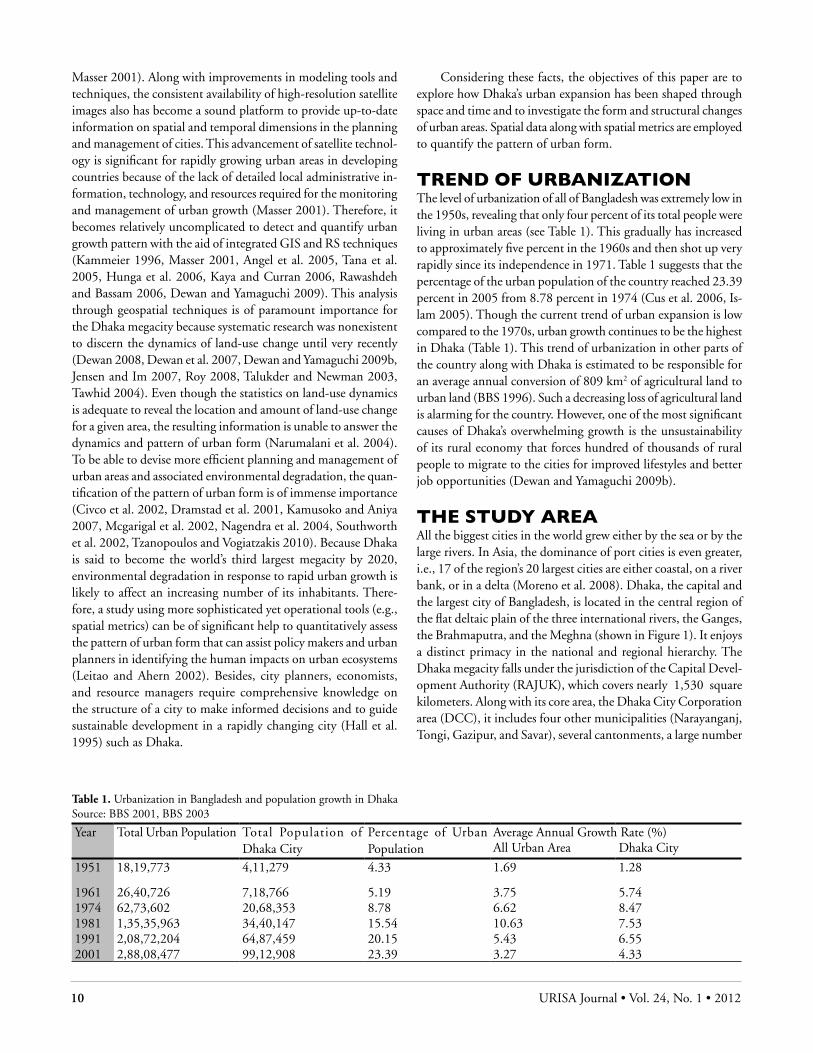
tREnd of URBAnIzAtIonThe level of urbanization of all of Bangladesh was extremely low in the 1950s, revealing that only four percent of its total people were living in urban areas (see Table 1). This gradually has increased to approximately five percent in the 1960s and then shot up very rapidly since its independence in 1971. Table 1 suggests that the percentage of the urban population of the country reached 23.39 percent in 2005 from 8.78 percent in 1974 (Cus et al. 2006, Is-lam 2005). Though the current trend of urban expansion is low compared to the 1970s, urban growth continues to be the highest in Dhaka (Table 1). This trend of urbanization in other parts of the country along with Dhaka is estimated to be responsible for an average annual conversion of 809 km2 of agricultural land to urban land (BBS 1996). Such a decreasing loss of agricultural land is alarming for the country. However, one of the most significant causes of Dhaka’s overwhelming growth is the unsustainability of its rural economy that forces hundred of thousands of rural people to migrate to the cities for improved lifestyles and better job opportunities (Dewan and Yamaguchi 2009b).
thE StUdy AREAAll the biggest cities in the world grew either by the sea or by the large rivers. In Asia, the dominance of port cities is even greater, i.e., 17 of the region’s 20 largest cities are either coastal, on a river bank, or in a delta (Moreno et al. 2008). Dhaka, the capital and the largest city of Bangladesh, is located in the central region of the flat deltaic plain of the three international rivers, the Ganges, the Brahmaputra, and the Meghna (shown in Figure 1). It enjoys a distinct primacy in the national and regional hierarchy. The Dhaka megacity falls under the jurisdiction of the Capital Devel-opment Authority (RAJUK), which covers nearly 1,530 square kilometers. Along with its core area, the Dhaka City Corporation area (DCC), it includes four other municipalities (Narayanganj, Tongi, Gazipur, and Savar), several cantonments, a large number
Table 1. Urbanization in Bangladesh and population growth in Dhaka Source: BBS 2001, BBS 2003
Year Total Urban Population Total Population of Dhaka City
Percentage of Urban Population
Average Annual Growth Rate (%)All Urban Area Dhaka City
1951 18,19,773 4,11,279 4.33 1.69 1.28
1961 26,40,726 7,18,766 5.19 3.75 5.741974 62,73,602 20,68,353 8.78 6.62 8.471981 1,35,35,963 34,40,147 15.54 10.63 7.531991 2,08,72,204 64,87,459 20.15 5.43 6.552001 2,88,08,477 99,12,908 23.39 3.27 4.33

URISA Journal • Ahmed, Bramley, Dewan 11
of rural settlements, massive wetlands areas, enormous agricultural lands, rivers, and part of the Modhupur forest of the Pleistocene period. Dhaka is mostly known by the boundary of the DCC and newly developed fringe areas of the DCC, also known as the Dhaka Statistical Metropolitan Area (DSMA) (Islam 2005). Dif-ferent roles of different institutions, different area connotations, and administrative and functional settings of Dhaka under mul-tiple organizational jurisdictions and responsibilities have made urban planning and development management in Dhaka highly fragmented and uncoordinated. The present metrogovernance of Dhaka has three types of agencies—national, sectoral, and local. Twenty-two ministries out of total 37 and 51 agencies are engaged in the city development and management of the Dhaka metropolitan area (ibid.). More information on city administration and governance structure can be found in Talukder and Newman 2003, Islam 2005. The population density has been the highest in the core areas (on average 14,000/km2), while the average for the extended development region (the gray-shaded area in Figure 1) is only 6,000 persons/km2, reflecting the fact
that only two-fifths of the megacity area is urban land. For a va-riety of reasons, including data constraints, this study considers the entire Dhaka metropolitan area (the bounding rectangle in Figure 1) instead of the whole Dhaka megacity (outer boundary in Figure 1).
Dhaka’s unique position as the country’s primary city and national administrative and economic capital makes it certain that future urbanization in Dhaka faces enormous spatial and socioeconomic challenges. In addition to its ever-increasing population triggered by rural to urban migration, its unplanned urban growth often is accompanied by the growth of massive informal settlements, congestion, and environmental pollution that are contributing to the degradation of the urban ecosystem. As a result, the city is expected to suffer more from flooding, waterlogging because of drainage congestion, and heat stress stemming from higher portions of built-up areas, higher popula-tion density, and increased industrial activities (Alam and Rab-bani 2007). Because Dhaka is located on very flat surfaces, the potential sea-level rise also remains an unknown but significant threat that could plunge many areas in the coming years. As far as the climate vulnerability is concerned, Dhaka is listed on the top, scoring highest among Asian cities (World Wild Life 2009).
dAtA And MEthodSData CollectionOnly recently, more rigorous efforts have been undertaken to monitor LUCC in Dhaka. Basak (2006) extracted multitemporal land-cover maps using LANDSAT images. His study covered the Dhaka Metropolitan Development Planning (DMDP) area. However, the outcome of the study suffered from low accuracy, and the result has not been calibrated nor validated. Dewan and Yamaguchi (2009) made a more precise attempt to identify spatiotemporal dynamics of LUCC for the Dhaka metropolitan area. They used a number of geospatial datasets from 1960 to 2005 (Ceo 2010, Dewan 2008, Dewan et al. 2007, Dewan and Yamaguchi 2009a, Dewan and Yamaguchi 2009b, Nasa 2010). The results of their studies were verified with historical maps and also with high-resolution remotely sensed images. Because it is the only verified and accessible source of LUCC data (derived through institutional arrangement) for most of the DSMA area, the bounding box as depicted in Figure 1 was selected as the case study area. A brief description on the acquisition and verification
Figure 1. The study area
Table 2. Description of land use/land cover for Dhaka Source: Dewan 2008, Dewan et al. 2007, Dewan and Yamaguchi 2009b
Land-use/Land-cover Types DescriptionBuilt-up Residential, commercial and services, industrial, transportation, roads, mixed urban, and other urbanBare soil/Landfill sites Exposed soils, landfills sites, and areas of active excavationCultivated land Agricultural area, crop fields, fallow lands, and vegetable landsVegetation Deciduous forest, mixed forest lands, palms, conifer, scrub, and othersWater bodies River, permanent open water, lakes, ponds, and reservoirsWetland/Lowlands Permanent and seasonal wetlands, low-lying areas, marshy land, rills and gully, swamps
12 URISA Journal • Vol. 24, No. 1 • 2012
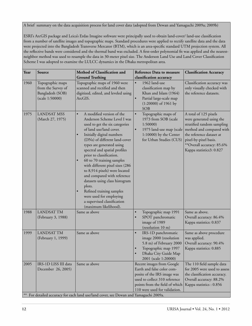
A brief summary on the data acquisition process for land cover data (adopted from Dewan and Yamaguchi 2009a; 2009b)
ESRI’s ArcGIS package and Leica’s Erdas Imagine software were principally used to obtain land-cover/ land-use classification from a number of satellite images and topographic maps. Standard procedures were applied to rectify satellite data and the data were projected into the Bangladesh Transverse Mercator (BTM), which is an area-specific standard UTM projection system. All the reflective bands were considered and the thermal band was excluded. A first-order polynomial fit was applied and the nearest-neighbor method was used to resample the data in 30-meter pixel size. The Anderson Land Use and Land Cover Classification Scheme I was adopted to examine the LULCC dynamics in the Dhaka metropolitan area.
Year Source Method of Classification and Ground Truthing
Reference Data to measure classification accuracy
Classification Accuracy
1960 Topographic maps from the Survey of Bangladesh (SOB) (scale 1:50000)
Topographic maps of 1960 were scanned and rectified and then digitized, edited, and leveled using ArcGIS.
• 1962 land-use classification map by Khan and Islam (1964)
• Partial large-scale map (1:20000) of 1961 by SOB
Classification accuracy was only visually checked with the reference datasets.
1975 LANDSAT MSS (March 27, 1975)
• A modified version of the Anderson Scheme Level I was used to get the six categories of land use/land cover.
• Initially digital numbers (DNs) of different land-cover types are generated using spectral and spatial profiles prior to classification.
• 60 to 70 training samples with different pixel sizes (286 to 8,914 pixels) were located and compared with reference datasets using class histogram plots.
• Refined training samples were used for employing a supervised classification (maximum likelihood).
• Topographic maps of 1973 from SOB (scale 1:50000)
• 1975 land-use map (scale 1:10000) by the Center for Urban Studies (CUS)
A total of 125 pixels were generated using the stratified random sampling method and compared with the reference dataset at pixel-by-pixel basis.**Overall accuracy: 85.6%Kappa statistics3: 0.827
1988 LANDSAT TM (February 3, 1988)
Same as above • Topographic map 1991 • SPOT panchromatic
image of 1989 (resolution 10 m)
Same as above. Overall accuracy: 86.4%Kappa statistics: 0.837
1999 LANDSAT TM (February 1, 1999)
Same as above • IRS-1D panchromatic image 2000 (resolution 5.8 m) of February 2000
• Topographic map 1997 • Dhaka City Guide Map
2001 (scale 1:20000)
Same as above procedure was applied. Overall accuracy: 90.4%Kappa statistics: 0.885
2005 IRS-1D LISS III data December 26, 2005)
Same as above Recent images from Google Earth and false color com-posite of the IRS image was used to collect 310 reference points from the field of which 110 were used for validation.
The 110 field sample data for 2005 were used to assess the classification accuracy. Overall accuracy: 88.2%Kappa statistics : 0.856
** For detailed accuracy for each land use/land cover, see Dewan and Yamaguchi 2009a.

URISA Journal • Ahmed, Bramley, Dewan 13
Figure 2. Flowchart showing the methodology of the study
tion matrix and/or with the spatial trend of a change detection tool. To be able to understand those questions, a large number of landscape metrics are available and being utilized to calculate spatial patterns of landscape properties (Kamusoko and Aniya 2007, Mcgarigal et al. 2002, Nagendra et al. 2004, Southworth et al. 2002, Tzanopoulos and Vogiatzakis 2010). However, these metrics are not able to characterize the spatial structure of a city, particularly historical urban form and pattern (Angel et al. 2007). To illustrate and quantify urban structure, the Urban Growth Analysis Tool (UGAT) has been employed in this study, which is predominantly useful to reveal the structure and form of a city (Angel et al. 2005). Because a number of metrics are available in UGAT, we used selected metrics pertinent to this study, and a brief description of each of the metrics is provided in the fol-lowing section.
Urban Manifestation Metrics This metric is specifically useful to understand whether a target pixel or group of pixels represents urban or not. This is known as urbanness. To derive urbanness, the percent of built-up pixels in a neighborhood is calculated by putting a one km2 circle in a given area. Then the area of all the pixels within a neighborhood is calculated and finally divided by the circle size (see Figure 3). Based on this calculation, urbanness can be subdivided into fur-ther categories such as main core, fringe, and scatter (Angel et al. 2007). If the largest contiguous group of pixels encompasses more than 50 percent built-up pixels (or >50 percent urbanness), it is termed urban core. In similar fashion, 30 percent to 50 percent urbanness near to the urban core is termed fringe areas, while areas with less than 20 percent urbanness are defined as scatter areas. A similar concept has been adapted to estimate the urbanness of the Dhaka metropolitan area.
New development metrics A number of metrics such as infill, extension, and leapfrog are embedded that demonstrate “new developments” for a given area. Using two periods of land-use data denoted as t
1 and t
2, new de-
velopments of a given area can be quantified. Infill is defined as the development of a small area surrounded by existing developed land. In other words, a nonurban pixel (e.g., vacant land) at time t
1 is converted to urban pixel at time t
2. The contiguity of a built-
up area increases with such type of development. Extension, on the other hand, is known as the outward development of existing urban areas. It is characterized by a nonurban pixel being converted
process of land use from these sources is provided in the text box. Details can be found in Dewan and Yamaguchi (2009a, 2009b).
The multi-temporal LUCC data (Dewan and Yamaguchi 2009a,b) were obtained through a formal agreement, and the product has been considered for further analysis to quantify the pattern of urban forms. It is necessary to note that the original land-use/land-cover data are in six categories—-urban, agricul-tural land, wetland, water bodies, forest/ vegetation, and bare soil (see Table 2).
MEthodoloGyA flowchart of the overall methods that were used in this study is presented in Figure 2. This study used two different approaches to quantify urban growth in terms of urban area change and measur-ing the specific aspect of urban structure. First of all, transition matrix, change statistics, and spatial trend of change have been employed using the Land Change Modeler Extension of ArcGIS (Clarke Lab 2008) to estimate spatial and temporal change in land use/land cover. To comprehend the contribution of other land-cover categories to the urban land of Dhaka, a transition matrix may be of particular importance. In addition, several polynomial trend surfaces4 were generated to detect the generalized trend of spatial change that is specifically useful to discern the pattern of change in different land-use/land-cover categories.
Simple analytical tools such as spatial trend of change or a transition matrix allow one to visualize locational changes and to derive necessary statistics to infer subjective judgment on the dynamics of land-use changes over longer periods. However these tools suffer from an unability to answer some fundamental ques-tions that a city planner needs to know. These are questions such as, what is the pattern of urban growth? How has the city evolved through different phases of development? How is urban growth affecting other land-use categories or what are the implications of such changes on overall urban environment? These are dif-ficult to answer and hard to quantify with a traditional transi-
Figure 3. Urbanness estimation (Angel et al. 2007, Angel et al. 2005)

14 URISA Journal • Vol. 24, No. 1 • 2012
to urban and surrounded by no more than 40 percent of existing urban pixels (Angel et al. 2007). Urban growth showing a scatter-ing of new development on isolated tracts separated from other areas of vacant land is defined as leapfrog (Ottensmann 1977), which is not intersecting the t
1 urban development. This type of
urban development results in a highly fragmented landscape in the periphery and supposedly has significant effects on the urban ecosystem (Angel et al. 2007).
Urban Extent Metrics While urbanness and new development metrics are useful to discern the spatial pattern of urban development, urban extent metrics, on the other hand, are particularly designed to map the spatial structure of a city. Using these metrics, we can easily perceive what constitutes a city. There are few metrics available under this heading. They are built-up area, urbanized area, urban-ized open space (OS), peripheral OS, and total OS. Each of these metrics provides useful information on the structure of a city. A short definition of each metric is given in Table 3.
Table 3. Summary of the metrics used for measuring the urban extent Source: Angel et al. 2007, Angel et al. 2005
Metric Definition
Built-up area Completely impervious surface (IS)
Urbanized areaBuilt-up area, including urbanized Open Space (OS)
Urbanized OSNonbuilt-up cells, neighborhood com-prised of more than 50% ofbuilt-up area
Peripheral OSNonbuilt-up cells that are within a distance of 100 m from built-uparea
Open space (OS) Total urbanized and peripheral OS
Urban footprint Built-up area with OS
Attributes of Urban Spatial Structure These are a set of metrics that are dedicated to quantify the compactness of a city. Urban form and pattern are supposed to change with each new development (e.g., an employment hub) in a rapidly urbanizing area. This type of activity leads to patches of noncontiguous urban cells, resulting in urban growth character-ized as leapfrog development (Angel et al. 2007, Angel et al. 2005). Because widespread leapfrogging reduces a city’s compactness, the estimation of compactness can allow a city planner to gauge one significant indicator of sustainable urban development. The compactness metric ranges from 0 to 1 in which higher values indicate more compact shape and vice versa. Three indices are used to measure the compactness of a city—the proximity index, the cohesion index, and the compactness index. The proximity index is based on the average distance of all points in the urbanized area to the centroid of the urbanized area. A circle with an area
equal to that of the urbanized area is used in proximity calcula-tion to normalize the distance values. While the cohesion index is based on the average distance between all possible pairs of points in an urbanized area, the compactness index uses the fraction of the shape area that is within an equal area circle centered at the shape certroid. Using these three metrics, one can possibly examine whether a city’s urban growth is resulting in pervasive sprawl, which is crucial information for a city planner.
RESUltS And dIScUSSIon
Initial Land-use/Land-cover Change Analysis
Amount of Change Figure 4 shows a summary on land-use/land-cover transforma-tions from 1960 to 2005 in the Dhaka metropolitan area. The LUCC statistics revealed that all land-use categories contributed significantly to make the urban land a predominant class, particu-larly after independence in 1971 (as captured by the land-cover data since 1975).
However, the principle contributors are the agricultural land and the wetlands in the recent past (see Figure 5). Prior to inde-pendence, agricultural land contributed most (more than 500 ha) to transform to urban land as the city started to increase its core by extending itself to surrounding agricultural land. Historical maps, the land use/land cover of 1961, the Master Plan of 1959, and literature confirmed that agricultural lands were the sources of urban developments during the 1970s (Basak 2006, Dewan and Yamaguchi 2009b, Islam 2005). However, urban growth did not gain its present momentum until its independence in 1971 when Dhaka regained its national capital status from provincial capital, and many administrative establishments took place that induced a rapid exodus from other districts. The city expanded almost six times in area between 1975 and 1988 as compared to in 1960–1975 (Dewan and Yamaguchi 2009a). Since then, it continues to proliferate at a constant pace of more than 1,000 ha/year during four observed periods. Apart from urban-land intensi-fication, the bare-soil/landfill category also increased considerably, portraying the pace of land development by the real estate agencies (Alam and Morshed 2010). In contrast, other land-use/land-cover classes, including water bodies, cultivated land, low-lying lands, and vegetation, have been reduced significantly to make way for built-up areas. In the 1970s and the 1980s, major development occurred mostly on cultivated lands. More than seven percent of these lands was converted to urban land, which increased nearly 13 percent in 1988, while the rate was only 2.23 percent during 1960–1975. Also, the built-up category expanded at an annual rate of 222 ha during 1975–1988, while the growth intensified steeply since the later half of the past century—with a rapid rate of more than 570 ha/year (see Figure 4). As mentioned earlier, agricultural land contributed more in all time periods (shown in Figure 5). Recent urban growth is being expanded onto low-lying areas, revealing that nearly 20 percent has been transformed to

URISA Journal • Ahmed, Bramley, Dewan 15
the built-up category from 1988 to 2005. While lowlands were not considered for urban development in earlier times, this type of land has become the major focus for urban expansion in the recent past, which should have a detrimental impact on the hydro-logical environment of the Dhaka metropolitan area. The major cause of lowland development can be explained by the fact that rapid population growth in the city requires more shelters, thus current urban expansion is being developed in the areas subject to seasonal flooding during monsoon.
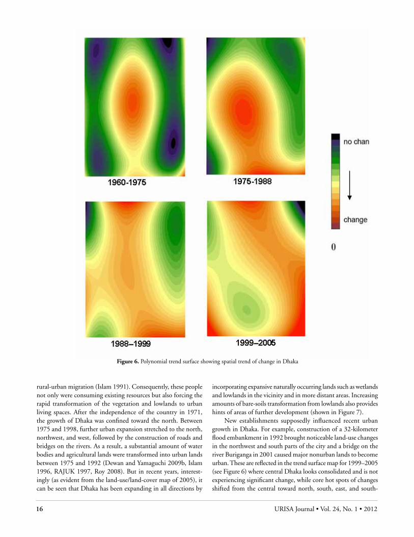
Locations of ChangePatterns of urban growth dynamics can be complex and thus
very difficult to decipher. The trend surface analysis in terms of best-fit polynomial can be used to detect the pattern of change from multitemporal land-use data. One of the polynomial trend surfaces of spatial change is shown in Figure 6. These surface maps depict a simulated surface where the values have no special significance but denote the generalized locations of transition between selected categories from areas with no change to areas with significant changes. Such a picture is useful to understand the generalized pattern of change and can assist in locating hot spots of land-use changes (i.e., areas for further investigation).
As mentioned earlier, Dhaka’s urban expansion was triggered mainly by rapid population growth originating from massive
Figure 4. Land-use/land-cover change (1960–2005)
Figure 5. Contribution of other land use/land cover to urban land (1960–2005)
16 URISA Journal • Vol. 24, No. 1 • 2012
rural-urban migration (Islam 1991). Consequently, these people not only were consuming existing resources but also forcing the rapid transformation of the vegetation and lowlands to urban living spaces. After the independence of the country in 1971, the growth of Dhaka was confined toward the north. Between 1975 and 1998, further urban expansion stretched to the north, northwest, and west, followed by the construction of roads and bridges on the rivers. As a result, a substantial amount of water bodies and agricultural lands were transformed into urban lands between 1975 and 1992 (Dewan and Yamaguchi 2009b, Islam 1996, RAJUK 1997, Roy 2008). But in recent years, interest-ingly (as evident from the land-use/land-cover map of 2005), it can be seen that Dhaka has been expanding in all directions by
incorporating expansive naturally occurring lands such as wetlands and lowlands in the vicinity and in more distant areas. Increasing amounts of bare-soils transformation from lowlands also provides hints of areas of further development (shown in Figure 7).
New establishments supposedly influenced recent urban growth in Dhaka. For example, construction of a 32-kilometer flood embankment in 1992 brought noticeable land-use changes in the northwest and south parts of the city and a bridge on the river Buriganga in 2001 caused major nonurban lands to become urban. These are reflected in the trend surface map for 1999–2005 (see Figure 6) where central Dhaka looks consolidated and is not experiencing significant change, while core hot spots of changes shifted from the central toward north, south, east, and south-
Figure 6. Polynomial trend surface showing spatial trend of change in Dhaka

URISA Journal • Ahmed, Bramley, Dewan 17
east directions in the 1990s and 2000s (third and fourth map, respectively, counterclockwise). Old maps and a number of field visits (Dewan and Yamaguchi 2009a) suggest that unplanned development is taking place to the east and northeast areas with the construction of new roads and services.
Dewan and Yamaguchi (2009a,b) pointed out that there was an uneven growth pattern in some directions during these periods. Both isolated and edge developments have become major features in the peripheral locations that have made the task harder for service-providing agencies to keep up the urban amenities in pace with the rapid urbanization of Dhaka. This lead to many environmental problems. For instance, the city becomes inun-dated during the monsoon season every year and waterlogging becomes a normal phenomenon with high flood risk potential because of the consistent encroachment and transformation of water bodies, wetlands, and lowland areas (Alam and Rabbani 2007, Dewan 2008, Huq 1999, Nishat et al. 2000). Furthermore, a large number of migrants taking their shelters in slum areas as housing is an acute problem in the city. Recent slum surveys confirm this hypothesis. For example, the number of people in slums already has doubled in a decade, revealing that the current slum population in Dhaka reached 3.4 million in 2006 from 1.5 million in 1995 (CUS et al. 2005). These slums, in most cases, are built near riverbanks and in areas highly vulnerable to envi-ronmental disasters. Not surprisingly, most of these slum dwellers are the ones most vulnerable when disasters such as floods strike
(Alam and Rabbani 2007, Cus et al. 2006, Islam 1999, Islam 2005, WB 2007).
AnAlySIS of URBAn foRM And StRUctURE Urban Manifestation The urban area of Dhaka has been explored by the manifestation metrics in terms of urban core, fringe, and scatter development based on the proportion of urbanness (see Figure 8). It is quite understandable from 1960 data that the city did not have any significant fringe and scatter developments because of its position as provincial capital. After the partition of India and Pakistan in 1947, there was more interest to have new administrative establishments rather than urban development. This lead to the creation of a Central Business District (CBD) and formal residential areas in the northwestern side of the city core. The city experienced major changes after the independence in 1971, resulting in extension and scatter developments in the 1970s.
The city continued to attract more people as time progressed and remained the primary city of Bangladesh. Major urban de-velopments were confined to the land free from inundation until 1990s. Figure 8 also shows that the urban fringe development was the highest in 1975, while current trend while current trend exhibit more scattering growth. Because of the absence of strict planning control, the city started to become more fragmented with
Figure 7. Changes from different land uses to urban (1988–2005)

18 URISA Journal • Vol. 24, No. 1 • 2012
more scattered development by the turn of this century, which are thought to have tremendous impact on the proper functioning of the ecosystem ( Huq 1999, Nishat 2000).
New Development Classification MetricsA timescale exploration over Dhaka’s evolution in terms of urban form and pattern is illustrated by Figure 9 and Table 4. Dhaka experienced its biggest leapfrog development once its status changed from provincial capital to national capital during the 1960–1975 period. Since then, extension of existing urban core development stretched while infill development remained relatively smaller. Leapfrogging started to take bigger proportions during the late 1990s when the main city core was consolidated, followed by higher land prices.
Little information is available to compare the results of this study with other cities in the world as published documents have not considered similar metrics. Attempt has been made to compare these outcomes with those already available for Bangkok, Thailand, and Minneapolis, Minnesota (Angel et al. 2007), so that the pattern and structure of Dhaka can be better understood. This has been accomplished without going further
into exploring or comparing the nature of the policy, physical, and socioeconomic structures and the changes of the concerned cities. The infill development in Dhaka is found to be lower than the infill development of both cities: Bangkok (27 percent) and Minneapolis (37 percent) while the extension of urban land has produced similar proportions during the time t4–t5 compared to that of Bangkok (63 percent) and Minneapolis (61 percent). One outstanding outcome is the leapfrogging of Dhaka, which is much higher than both cities (see Table 4). This clearly shows that Dhaka’s recent urban expansion is a result of isolated land developments away from the urban core. This contradicts the findings of Richardson et al. (2000) that cities in developing countries are becoming more compact. In the case of Dhaka, though the city has a trend to compactness in an earlier time, the recent trend is toward dispersion through leapfrog development.
Urban Extent Metrics Summary statistics on urban extent metrics has been calculated for a total timescale 1960–2005 in percentages (shown in Table 5). This resulted in sharp differences in terms of statistics. An-nual average conversion to urban areas has been 353.874 ha for
Figure 8. Urban manifestation metric for Dhaka (1960–2005)

URISA Journal • Ahmed, Bramley, Dewan 19
the total timescale while that has been higher than 216 ha for the period 1988–2005 (shown in Table 5). Even though the amount of urbanized area (that includes built-up area and open space within the urban core) has escalated over both timescales, the amount of urban open space has depleted substantially in both cases. This event happened similarly for peripheral open spaces as the urban core continued to expand and leapfrog to the peripheral (see Figure 10). This has resulted in the rapid decline of open spaces from 42 percent of open spaces to about eight percent in the late 20th century. This has been in stark contrast to the findings for Bangkok where open space has increased by two percent and in Minneapolis where open space has declined only slightly (0.1 percent) (Angel et al. 2007).
Attributes of Urban Spatial Structure The spatial structure of the city can be estimated in terms of proximity, cohesion, and the compactness index (see Table 6). The
Figure 9. Urban form metrics in Dhaka (1960–2005)
analysis revealed that proximity and the cohesion index are con-sistently higher since 1960 except for the year 1975. This is true for the average distance between all pairs of urban cells (shown in Table 6). Looking into the spatial size of Dhaka’s urban land in 1960 would clear up any confusion as until then, it had been a small compact town. But since Dhaka’s independence in 1971, its urban footprint has become fragmented by outward exten-sion and leapfrogging, thus increasing the average travel distance and lowered index value in 1975. Compactness had been found lower compared to that in 1960 for the edges of built-up areas expanded, resulting in more urbanized open space and making it less compact. But since then, it has started to increase as built-up areas started to consolidate in most areas, thus reducing the average travel distance. Bangkok has been found less compact than Dhaka (0.44 in 1994 and 0.51 in 2002), while Minneapolis has been more consolidated (0.77 in 1992 and 0.81 in 2001) (Angel et al. 2007).

20 URISA Journal • Vol. 24, No. 1 • 2012
conclUdInG REMARkSThe objective of this study was to quantify the urban form and structure of Dhaka using multitemporal land-use/land-cover data since 1960. A variety of spatial metrics were employed to discern form and pattern of urban change. Using UGAT, a number of metrics were calculated to reveal the structure of the city. The results revealed that Dhaka experienced and witnessed rapid conversion of agricultural and low-lying areas in the recent past. Consequently, urban areas have been increased to a greater extent. The total urban footprint quickly grew to 20,551.0 ha (49.4 percent of the total land mass) in 2005 from 4,631.8 ha (11.1 percent) in 1961—converting 3,000 ha of agricultural land during 1975–1988 alone. Although the initial growth was confined to the northern part of the city core, core hot spots of changes shifted from the central toward the north, south, east, and southeast directions in the 1990s and 2000s as exemplified initially by the trend surface and later by the tables and maps
Table 4. Urban form metrics of Dhaka (1960–2005)
Metrics t1-t2(1960–1975)
t2-t3(1975–1988)
t3-t4(1988–1999)
t4-t5(1999–2005)
NewUrbanGrowth
ha 2411.910 6608.610 6885.450 6920.730
% 100.00 100.00 100.00 100.00
Infillha 266.67 978.66 1468.53 1467.00
% 11.06 14.81 21.33 21.20
Extensionha 1173.60 4720.59 5012.73 4517.28
% 48.66 71.43 72.80 65.27
Leapfrogha 971.64 909.36 404.19 936.45
% 40.29 13.76 5.87 13.53
Table 5. Metrics for measuring urban extent of Dhaka (1960–2005)
Metricst1(1960)
t2(1975)
t3(1988)
t4(1999)
t5(2005)
Built-up Area71.80 57.59 77.65 91.70 91.44
Urbanized Area75.89 64.55 81.56 93.53 92.93
Urbanized OS4.08 6.95 3.91 1.83 1.49
Urban Footprint100.00 100.00 100.00 100.00 100.00
Peripheral OS24.11 35.45 18.44 6.47 7.06
Open Space28.19 42.40 22.35 8.30 8.56
and also confirmed by previous literature. Locations of these changes are further explored with UGAT tools. Nevertheless infill development continues and stays substantial even after sufficient consolidation already had taken place, which can be attributed mainly to the nonshifting nature of principal jobs and the com-mercial hub located here and shorter work-home trip lengths in Dhaka (also evident from the proximity and cohesion index). This already has placed a huge strain on inner open spaces and these are continuously dwindling. The most occurring changes are taking place through the extension of existing urban footprints while leapfrogging also is taking a fair share.
These are useful insights for city planners for the city who do not have up-to-date data or information over the rapid transforma-tion in LUCC that Dhaka is experiencing. With the absence of a reliable, up-to-date, accurate city land-use database for Dhaka, such land-use maps (as used in this study) can assist as efficient instruments for the urban development information system,

URISA Journal • Ahmed, Bramley, Dewan 21
which seems a prerequisite to land-use planners and decision makers for sustainable management and growth of an extended megacity region such as greater Dhaka. This explorative analysis with the urban growth metrics (UGAT) has been helpful in look-ing into the changing urban form of Dhaka for more than nearly half a century. It provides some clues on how the city core has expanded over time and fragmented other land uses previously found dominant, plus when and where leapfrogging has been acting as seeds of growth in later periods. These insights will as-sist in making realistic simulations for Dhaka in future scenario analyses made by researchers. More of such applications means better assistance to planners and decision makers in these countries to obtain a better knowledge about urban land-use dynamics and the pattern of urban growth. Recent urban growth also is associ-ated with the massive land speculation, especially in the fringe of suburban areas. Soaring land prices coupled with increasing demand for housing and land development has outweighed the
Figure 10. Urban extent metrics for Dhaka (1960–2005)
Table 6. Attributes of urban spatial structure for Dhaka (1960–2005)
Metrics 1960 1975 1988 1999 2005
Proximity Index 0.77 0.65 0.76 0.78 0.82
Cohesion Index 0.74 0.63 0.75 0.77 0.81
Compactness index 0.74 0.58 0.65 0.66 0.68
high value of some agricultural lands in the fringe, with some of this land becoming rapidly urban through individual and property developers (Dewan 2009a). There might be factors other than land price and speculation influencing such complex processes in the suburban areas and this, therefore, necessitates detailed study that can explore underlying drivers determining urban growth in the Dhaka megacity.
Notes
1Assuming the population at 2015 as 15 million, this is a 20-year (1995–2015) strategy plan for urban development within the Capital City Development Authority’s jurisdiction. It consists of a report with supporting policy maps (RAJUK 1997).
2On the other hand, this is an interim midterm plan from 1995 to 2005 and covers a smaller area than the former, e.g., existing metropolitan area of Dhaka (RAJUK 1997).
22 URISA Journal • Vol. 24, No. 1 • 2012
3Kappa coefficient is a statistical measure of interannotator agree-ment for qualitative (categorical) items. It generally is thought to be a more robust measure than simple percent agreement calculation for it takes into account the agreement occurring by chance.
4The procedure is not without drawbacks and the main ones are: difficult to interpret individual terms, hugely biased to edge effects, and rarely goes through data points (i.e., inexact in-terpolator). Nevertheless, it has some practical rationale for wider applications: easy to compute and hides finer pockets of variations to display general or average trends across the landscape (by detrending the data) (Smith et al. 2007).
Acknowledgment
This research was part of the Doctoral Programme in Urban Studies at the Heriot-Watt University, Edinburgh, UK. The authors would like to thank the ORS & James Watt Scholarship for funding the study.
About the Authors
Sohel J. Ahmed completed his Ph.D. from Heriot-Watt University, Edinburgh, UK. He received his Master’s in Geoinformation Science and Earth Observation from the University of Twente, the Netherlands. His research interest includes spatial analysis, decision support systems, multi-criteria evaluation, and land-use modeling. He currently is conducting postdoctoral research as a land-use modeller and spatial analyst at the School of GeoSciences, University of Edinburgh, UK.
Corresponding Address: Crew Building, the King’s Buildings School of GeoSciences University of Edinburgh Edinburgh, UK [email protected] www.geos.ed.ac.uk
Glen Bramley is a professor of Urban Studies at Heriot-Watt University in Edinburgh, where he leads a substantial research program in housing and urban studies. His recent work is focused particularly on planning for new housing, housing need, home ownership, neighborhood change, urban form, quality of life, poverty, and the funding and outcomes of local services. His publications include Key Issues in Hous-ing (Palgrave 2005) and Planning, the Market and Private Housebuilding (UCL Press 1995).
Ashraf Dewan is a lecturer in GI Sciences at Curtin University, Western Australia. He is also an associate professor in the Department of Geography and Environment, University of Dhaka. He completed his Ph.D. on Environmental En-gineering from Okayama University, Japan. His research
interest includes GIS/RS, spatial analysis, climate change, and health issues.
References
Aguilar, A. G., and P. M. Ward. 2003. Globalization, regional development, and mega-city expansion in Latin America: Analyzing Mexico City’s peri-urban hinterland. Cities 20: 3-21.
Alam, M., and M. D. G. Rabbani. 2007. Vulnerabilities and responses to climate change for Dhaka. Environment and Urbanization 19: 81-97.
Alam, M. J., and M. M. Ahmad. 2010. Analysing the lacunae in planning and implementation: spatial development of Dhaka city and its impacts upon the built environment. International Journal of Urban Sustainable Development 2(1 and 2): 85-106.
Angel, S., J. Parent, and D. Civco. 2007. Urban sprawl metrics: An analysis of global urban
expansion using GIS. ASPRS Annual Conference. May 7-11, Tampa, Florida.
Angel, S., S. C. Sheppard, and D. L. Civco. 2005. The dynamics of global urban expansion. In Transport and Urban Develop-ment Department . The World Bank, Washington D.C..
Angeles, G., P. Lance, J. Barden-O’fallon, N. Islam, A. Mahbub, and N. I. Nazem. 2009. The 2005 census and mapping of slums in Bangladesh: Design, selected results and application. International Journal of Health Geographics 8:32 http://www.ij-healthgeographics.com/content/8/1/32 (accessed on 20.3.2010)
Basak, P. 2006. Spatio-temporal trends and dimensions of urban form in central Bangladesh: A GIS and remote sensing analy-sis. MSc Dissertation, Bangladesh University of Engineering and Technology (BUET), Dhaka.
Batty, M. 2001. Models in planning: Technological imperatives and changing roles. International Journal of Geo-information Science and Earth Observation 3: 252-66.
Batty, M. 2005. Agents, cells, and cities: New representational models for simulating multiscale urban dynamics. Environ-ment and Planning A 37: 1373-94.
BBS. 1996. Agricultural census of Bangladesh. Bangladesh Bureau of Statistics & Ministry of Planning, Dhaka.
BBS. 2001. Statistical yearbook of Bangladesh. Bangladesh Bureau of Statistics & Ministry of Planning, Dhaka.
BBS. 2003. Population census 2001. Bangladesh Bureau of Sta-tistics & Ministry of Planning.
CEO. 2010. Obtaining and Importing Landsat Data. The Center for Earth Observation (CEO), Yale University.
Civco, D. L., J. D. Hurd, E. H. Wilson, C. L. Arnold, and S. Prisloe. 2002. Quantifying and describing urbanizing land-scapes in the northeast United States. Photogrammetric Engineering and Remote Sensing 68: 1083-90.

URISA Journal • Ahmed, Bramley, Dewan 23
Clark Labs. 2008. Land Change Modeler extension for ArcGIS. Clark University, U.S.
CUS, NIPORT, and MEASURE. 2006. Slums in urban Bangla-desh: Mapping and census, 2005. Center for Urban Studies (CUS), National Institute of Population, Research and Training (NIPORT), and MEASURE Evaluation, Dhaka.
Dewan, A. M., and Yamaguchi, Y. 2008. Effect of land cover changes on flooding: Example from Greater Dhaka of Ban-gladesh. International Journal of Geoinformatics 4: 11-20.
Dewan, A. M., M. M. Islam, T. Kumamoto, and M. Nishigaki. 2007. Evaluating flood hazard for land-use planning in greater Dhaka of Bangladesh using remote sensing and GIS techniques. Water Resource Management 21: 1601-12.
Dewan, A. M., and Y. Yamaguchi. 2009a. Using remote sens-ing and GIS to detect and monitor land use and land cover change in Dhaka metropolitan of Bangladesh during 1960–2005. Environmental Monitoring and Assessment
150: 237-49.Dewan, A. M., and Y. Yamaguchi.. 2009b. Land use and land
cover change in Greater Dhaka, Bangladesh: Using remote sensing to promote sustainable urbanization. Applied Ge-ography 29 (3):390-401.
Dramstad, W. E., G. Fry, W. Fjellstad, B. Skar, W. Helliken, M. L. B. Sollund, M. Streit, A. K. Geelmuyden, and E. Frams-tad. 2001. Integrating landscape-based values— Norwegian monitoring of agricultural landscapes. Landscape and Urban Planning 57: 257-68.
Goodchild, M. F. 2005. GIS and modeling overview. In Magu-ire, D. J., M. Batty, and M. F. Goodchild, Eds. GIS, spatial analysis, and modeling. ESRI Press, pp. 1-18.
Hardin, P. J., M. W. Jackson, and S. M. Otterstrom. 2007. Map-ping, measuring, and modeling urban growth. In Jensen, R R., J. D. Gatrell, and D. McLean, Eds. Geospatial tech-nologies in urban environments: Policy, practice and pixels. Springer-Verlag, pp. 141-76.
Huq, S. 1999. Environmental problems of Dhaka City. In Mitch-ell, J. K., Ed. Crucibles of hazard: Mega-cities and disasters in transition. United Nations University Press, p. 544.
Islam, N. 1991. Dhaka in 2025 AD. In S. Ahmed, Ed. Dhaka: Past, present and future. The Asiatic Society of Bangladesh, pp. 570-83.
Islam, N. 1996. High class residential areas in Dhaka city, 1608-1962. In Islam, N. E., Ed. Dhaka—from city to megacity: Perspectives on people, places, planning and development issues. Bangladesh Urban Studies Series No. 1., Urban Studies Programme( USP), Department of Geography, University of Dhaka, p. 241.
Islam, N. 1999. Dhaka city: Some general concerns. Asian cities in the 21st century: Contemporary approaches to municipal management. Asian Development Bank (ADB), pp. 71-82.
Islam, N. 2005. Dhaka now: Contemporary urban development. The Bangladesh Geographical Society, Dhaka.
Jensen, J. R., and J. Im. 2007. Remote sensing change detection in urban environments. In Jensen, R. R., J. D. Gatrell, and D. McLean, Eds. Geo-spatial technologies in urban environ-ments: Policy, practice and pixels. Springer-Verlag, pp. 7-30.
Kamusoko, C., and M. Aniya. 2007. Land use/cover change and landscape fragmentation analysis in the Bindura District, Zimbabwe. Land Degradation and Development 18: 221-33.
Kok, K., P. H. Verburg, and T. A. Veldkamp. 2007. Integrated assessment of the land system: The future of land use. Edito-rial. Land Use Policy 24: 517-20.
Kötter, T. 2004. Risks and opportunities of urbanization and mega-cities. Plenary Session 2 - Risk and Disaster Prevention and Management in In ternational Federation of Surveyors (FIG) Working Week. May 22-27, Athens, Greece.
http://www.fig.net/pub/athens/papers/ps02/ps02_2_kot-ter.pdf(accessed on 23.3.2010)
Kraas, F. 2003. Mega-cities as global risk areas. Petermanns Geographische Mitteilungen (PGM) 147: 6-15.
Leitao, A. B., and J. Ahern. 2002. Applying landscape ecologi-cal concepts and metrics in sustainable landscape planning. Landscape and Urban Planning 59: 65-93.
Masser, I. 2001. Managing our urban future: The role of remote sensing and geographic information systems. Habitat Inter-national 25: 503-12.
Mcgarigal, K., S. A. Cushman, M. C. Neel, and E. Ene. 2002. FRAGSTATS: Spatial Pattern
Analysis Program for Categorical Maps. Computer software program produced by the authors at the University of Massa-chusetts, Amherst. Available at the following web site: http://www.umass.edu/landeco/research/fragstats/fragstats.html
Moreno, E. L., N. Bazoglu, G. Mboup, and R. Warah. 2008. State of the world’s cities 2008/2009: Harmonious cities. In Warah, R., Ed. United Nations Human Settlements Programme ( UN-Habitat), p. 280.
Nagendra, H., D. K. Munroe, and J. Southworth. 2004. From pattern and process: Landscape fragmentation and the analysis of land use/cover change. Agriculture, Ecosystem and Environment 101: 111-15.
Narumalani, S., D. R. M. Mishra, and R. G. Rothwell. 2004. Change detection and landscape metrics for inferring an-thropogenic processes in the greater EFMO area. Remote Sensing of Environment 91: 478-89.
NASA. 2010. Landsat then and now. National Aeronautics and Space Administration.
Nishat, A., M. Reazuddin, R. Amin, and A. R. Khan. 2000. The 1998 flood: Impact on environment of Dhaka city. Depart-ment of Enviornment, IUCN–Bangladesh.
Ottensmann, J. R. 1977. Urban sprawl, land values and the den-sity of development. Land Economics 53: 389-400.
RAJUK. 1997. Dhaka metropolitan development plan for Dhaka city (1995–2015). Vols. I and II. Rajdhani Unnayan Kat-ripakkha (RAJUK).

24 URISA Journal • Vol. 24, No. 1 • 2012
Repetti, A., and R. Prelaz-Droux. 2003. An urban monitor as support for a participative management of developing cities. Habitat International 27: 653-67.
Rindfuss, R. R., S. J. Walsh, B. L. Turner II, J. Fox, and V. Mishra. 2004. Developing a science of land change: Challenges and methodological issues. PNAS 101(13):976-981.
Roy, M. 2008. Planning for sustainable urbanisation in fast growing cities: Mitigation and adaptation issues addressed in Dhaka, Bangladesh. Habitat International 33(3): 276–286
Siddiqui, K. 2004. Megacity governance in South Asia: A com-parative study. University Press Limited (UPL), Dhaka.
Smith, M. J. D., M. F. Goodchild, and P. A. Longley. 2007. Geospatial analysis: A comprehensive guide to principles, techniques and software tools, 2nd Ed.University College London (UCL), London.
Southworth, J., H. Nagendra, and C. Tucker. 2002. Fragmenta-tion of a landscape: Incorporating landscape metrics into satellite analysis of land cover change. Landscape Research 27: 263-69.
Talukder, S. H., and P. Newman. 2003. In search of sustainable governance and development management setting for a megacity and its extended metropolitan region (EMR): The case study of Dhaka—capital of Bangladesh. Proceedings of the International Sustainability Conference Government of Western Australia.
Tawhid, K. G. 2004. Causes and effects of water logging in Dhaka City, Bangladesh. MSc Dissertation, Royal Institute of Technology (KTH), Stockholm.
Tzanopoulos, J., and I. N. Vogiatzakis. 2010. Processes and pat-terns of landscape change on a small Aegean island: The case of Sifnos, Grecce. Landscape and Urban Planning 99: 58-64.
Verburg, P. H., P. Schot, M. J. Dijst, and A. Veldkamp. 2004. Land use change modelling: Current practice and research priorities. GeoJournal 61: 309-24.
World Bank. 2007. Dhaka: Improving living conditions for the urban poor. Bangladesh Development Series. Sustainable Development Unit, South Asia Region, The World Bank, p. 1578.

URISA Journal • Broitman, Czamanski 25
IntRodUctIonClassical models of urban spatial structure (Alonso 1964, Mills 1967, Muth 1969) depict cities as monocentric. They view real cities at a crude resolution only. To this end, they utilize aver-age densities (Alperovich and Deutsch 2000). In these models, people and activities compete for space and locations in terms of proximity to a single city center. The competition leads to monotonically declining land rents and density from the central business district (CBD) outward (Fujita 1989). Such models are hard-pressed to explain the formation of modern cities with the typical polycentric structure.
Recent research concerned with urban spatial dynamics suggests that discontinuity in space and nonuniformity in time are prominent characteristics of modern urban development (Benguigui et al. 2001a, 2001b, 2004a, 2004b, 2006). Thus, for example, the footprint of the built area in the Tel Aviv conurba-
Polycentric Urban dynamics—heterogeneous developers under certain Planning Restrictions
Dani Broitman and Daniel Czamanski
Abstract: The paper is concerned with the formation of polycentric cities. The model we introduce includes two types of developers and planning authorities. Developers’ characteristics, such as scale of operations, availability of own capital, and time preferences, lead to various decisions concerning the choice of location and development investment. They are influenced by planners’ deci-sions concerning developable locations. We present a cellular automaton model that simulates the interaction of various types of developers and planning authorities. We demonstrate that the joint dynamics of decisions by impatient, low-scale developers with others who are willing to wait a long time to realize returns on their investment can lead to the creation of new urban subcenters.
tion displays discontinuity that appears as a result of apparent leapfrogging (see Figure 1).
Furthermore, the evolution of high-rise buildings represents evidence contrary to the monocentric paradigm. There is some evidence that clustering of high-rise buildings over time is weaken-ing (Golan 2009). Quantitative measures indicate that no single urban center of attraction is present in the city (Czamanski and Roth 2011). Moreover, new high-rise building clusters seem to arise over time in zones previously not intensively developed (Golan 2009).
In an effort to explain the apparent discontinuities in the spa-tial evolution of built areas, we argue that the polycentric structure results from the behavior of developers that incorporate the prefer-ences of consumers (Henderson et al. 2008) together with measures taken by planning authorities. The planning actions consist of land-use plans intended to prevent unwanted urban development in areas reserved for nature, parks, recreation, and agriculture (Furst et al. 2010). The effectiveness of land-use plans is related to the ability of planning boards to withstand the pressure of developers to convert land that is not intended for development and was purchased by developers at a low market price into high-proceeds developable land (Lai et al. 2008). While the ability of developers to influence planning boards and to obtain planning variances varies among countries, it is a universal phenomenon. As we shall demonstrate in this paper, the resistance of planning boards is directly responsible for sprawl in the form of leapfrogging.
The overall purpose of this paper is to incorporate planning decisions into an agent-based simulation model that yields realistic urban spatial structures. It is our claim that the combined effect of urban planning policies and regulations and the choices of developers searching for real estate projects can explain much of the urban spatiotemporal evolution. Firm characteristics, and in particular the time impatience of land developers, interacts with time-related municipal development strategies and, in turn, affects the urban spatial structure dynamics.Figure 1. The temporal evolution of Tel-Aviv’s footprint

26 URISA Journal • Vol. 24, No. 1 • 2012
The rest of this paper consists of three more sections. The next section contains a description of our model. The following section present results of model simulations. The last section pres-ents discussion of our results and suggestions for future research.
ModEl dEScRIPtIonWe present an agent-based model with two main types of agents. Planning authority sets rules concerning the location and in-tensity of developable land. We assume that planning building restrictions grow with distance from the central business district (CBD). These restrictions are expressed as a monotonically increasing function of the time required for obtaining construc-tion permits as the distance from the CBD increases. From the developers’ point of view, this is the time between the acquisi-tion of property rights and the realization of returns. We define it as the characteristic time of a given location. Developers are the second type of agents. They select preferred locations for buildings and the intensity, or height, of buildings. We define two types of real estate developers. The first type is an impatient developer, characterized by small-scale operations resulting in low and medium-height buildings and a preference for immediate returns on investment, thus “small” developers. The second type is a patient developer, characterized by financial capabilities, an ability to wait long periods to maximize returns on investment, and large-scale development operations (high-rise buildings), thus “big” developers.
As we shall illustrate in the following, the presence of one homogenous group of “small” developers results in an Alonso-type monocentric city. Most cities, however, display a polycentric structure (Czamanski and Roth 2011). In our model, we generate polycentric structure by including a mix of small developers and large patient developers. As long as land is available for develop-ment within a radius with characteristic time that is below or equal to the developers’ time impatience, building will proceed and the competition for accessibility will generate an Alonso-type city. This circular-shaped monocentric city has a radius directly related to the characteristic time function imposed by the planning authorities. As available land in the monocentric city is exhausted, pent-up demand will cause willingness to pay to rise. Some of the small developers with a preference for immediate returns on investments will leave the sector of land development and turn to other activities. A period of building stagnation without significant construction activity will follow.
However, some large developers, patient enough to wait for long-term returns, will speculate and purchase low-priced land for future development. This land is in areas with high charac-teristic time. They will hold the land until the characteristic time will elapse and building will be possible. By waiting it out, the big developers will achieve a return on investment that is higher than in the core of the city. Also, they will purchase old buildings within the pale of the CBD that can be demolished and thus make land available for high-rise modern structures. Because of historic preservation constraints, limited and outdated urban
infrastructure, and opposition from neighbors, the characteristic time of these sites is high.
When many parcels of speculatively bought land are concentrated in a particular region, the planning authorities acknowledge that the region is being urbanized despite the high characteristic times imposed in it and, with some probability, reduce the characteristic time around this new development pole. Small developers with a preference for immediate returns on investments are attracted to the region and start building as well. A new Alonso-type urban center will be created.
The timing of the peaks and troughs in construction activities is a function of the size and the rate of change in the characteristic time. The number, size, and speed of construction of subcenters depend on the relative number of the two types of developers and the city development policies regarding the characteristic time. Big developers get out of development business and get back, into both speculative and construction activities, following the external economic cycles. There may be a delay and each type of activity can depend on different characteristics of the cycle.
Our spatial, agent-based simulation model displays the city spatial configuration in each time step. The city is defined as a square grid of cells, each of which represents a single parcel of land. The cells’ status in any given time step is characterized by several attributes:
Characteristic Time The time delay imposed on each specific cell by city authorities on potential developers from the time that property rights are purchased and until the project construction and revenue realiza-tions. This attribute is a function of location. Also, characteristic time increases with height. (See Figure 2.)
Cell Use Status One of the following three statuses is possible: available (not de-veloped), purchased (waiting for the characteristic time elapsing and, therefore, not developed yet), or developed (an occupied cell with a building standing in it). Status can change over time.
Figure 2. City’s transect at the initial stage—single CBD and increasing characteristic time
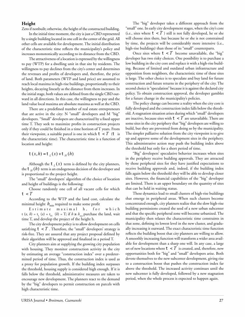
URISA Journal • Broitman, Czamanski 27
Height Zero if nonbuilt; otherwise, the height of the constructed building.
In the initial time moment, the city is just a CBD represented by a single building located in one cell in the center of the grid. All other cells are available for development. The initial distribution of the characteristic time reflects the municipality’s policy and increases monotonically according to its distance from the CBD.
The attractiveness of a location is expressed by the willingness to pay (WTP) for a dwelling unit in that site by residents. The willingness to pay declines from the city’s center and determines the revenues and profits of developers and, therefore, the price of land. Both parameters (WTP and land price) are assumed to reach local maxima in high-rise buildings, proportionally to their heights, decaying linearly as the distance from them increases. In the initial stage, both values are defined from the single CBD out-ward in all directions. In this case, the willingness to pay and the land value local maxima are absolute maxima as well at the CBD.
There are a predefined number of real estate entrepreneurs that are active in the city: N “small” developers and M “big” developers. “Small” developers are characterized by a fixed upper time T. They seek to maximize profits in construction projects only if they could be finished in a time horizon of T years. From their viewpoint, a suitable parcel is one in which T<t (t is the characteristic time). The characteristic time is a function of location and height:
)()(),( hxhx HL ttt +=
Although the )(xLt term is defined by the city planners, the )(hHt term is an endogenous decision of the developer and is proportional to the project height.
The “small” developers’ algorithm of the choice of location and height of buildings is the following:
Choose randomly one cell of all vacant cells for which T<tAccording to the WTP and the land cost, calculate the
minimal height minh required to make some profitE s t i m a t e m a x i m a l h , f o r w h i c h
t (x, h) = tL (x) + t
H (h) = T; if h ≥ h
mn purchase the land, wait
time T, and develop the project of the height h.The city development policy is to allow development on cells
satisfying T<t . Therefore, the “small” developers’ strategy is risk-free. They are assured that any project proposal defined by their algorithm will be approved and finalized in a period T.
City planners aim at supplying the growing city population with housing. They monitor construction activity in the city by estimating an average “construction index” over a predeter-mined period of time. Thus, the construction index is used as a proxy for population growth. If the building index surpasses the threshold, housing supply is considered high enough. If it is falls below the threshold, administrative measures are taken to encourage new development. The planners react to the demand by the “big” developers to permit construction on parcels with high characteristic time.
The “big” developer takes a different approach from the “small” one. In early city development stages, when the city’s core (i.e., sites where T<t ) still is not fully developed, he or she will choose sites there, but because he or she is not constrained by time, the projects will be considerably more intensive (i.e., high-rise buildings) than those of its “small” counterparts.
Once sites where T<t become unavailable, the “big” developer has two risky choices. One possibility is to purchase a low building in the city core and replace it with a high-rise build-ing. Because of limited and outdated urban infrastructure and opposition from neighbors, the characteristic time of these sites is large. The other choice is to speculate and buy land for future construction and future returns in the periphery of the city. The second choice is “speculation” because it is against the declared city policy. To obtain construction approval, the developer gambles for a future change in the municipality’s policies.
The policy change can become a reality when the city core is fully developed and the construction index falls below the thresh-old. A stagnation situation arises during which “small” developers are inactive, because sites with T<t are unavailable. There are some sites in the city periphery that “big” developers are willing to build, but they are prevented from doing so by the municipality. The simpler palliative solution from the city viewpoint is to give up and approve some of the development sites in the periphery. This administrative action may push the building index above the threshold but only for a short period of time.
“Big” developers’ speculative behavior increases when sites in the periphery receive building approvals. They are attracted by those peripheral sites for they have justified expectations to receive building approvals and, indeed, if the building index falls again below the threshold they will be able to develop closer sites. However, the financial capabilities of the “big” developer are limited. There is an upper boundary on the quantity of sites that can be held in waiting status.
These dynamics lead to small clusters of high-rise buildings that emerge in peripheral areas. When such clusters become concentrated enough, city planners realize that the slow high-rise building permissions created the seed of a new urban subcenter and that the specific peripheral zone will become urbanized. The municipality then relaxes the characteristic time constraints in that zone, defining its lowest level in the new cluster, and gradu-ally increasing it outward. The exact characteristic time function reflects the building boost that city planners are willing to allow. A smoothly increasing function will transform a wider area avail-able for development than a sharp one will. In any case, a large set of new locations where T<t is created, and, therefore, new opportunities both for “big” and “small” developers arise. Both devote themselves to the new subcenter development, giving rise to a construction boost that pushes the construction index far above the threshold. The increased activity continues until the new subcenter is fully developed, followed by a new stagnation period, when the whole process is expected to happen again.

28 URISA Journal • Vol. 24, No. 1 • 2012
The main model elements are described in the following list:• Economic parameters: Willingness to pay, land price, and
the rate of decay with distance. These parameters are kept fixed in all the scenarios described here.
• Developers composition (number of “small” and “big” developers active in the city). Different developers’ composition will lead to different spatial results.
• City planners monitoring and policy tools: Building index over time and policy-setting parameters. Most of these parameters are kept fixed in all the analyzed scenarios. The only one that is changed is the size of the area allowed for development when a new peripheral area is urbanized.The following Table 1 summarizes the model’s parameters:
RESUltSMost model parameters are kept fixed during all the scenarios runs. Only a selected group of parameters are changed to allow sensitivity tests. Those key parameters are the relative number of “small” and “big” developers and the area defined for a new urbanization pole once the authorities decide to allow develop-ment in a previously open periurban space. Within each scenario each key parameter is specified.
In all the following simulations a high characteristic time function is assumed.
fIRSt ScEnARIo: hoMoGEnEoUS dEvEloPERSIn the presence of a homogenous group of “small” developers, the cityscape resembles an Alonso-type city. The city size and its height
distributions depend on the development policy implemented by planning authorities. Assuming a single development strategy (will-ingness to concentrate urban development around the existing city core and prevent sprawl), three different policy settings are explored: a constrictive setting characterized by high characteristic times, a more relaxed setting with medium times, and an expansive policy using low characteristic times. In all three cases, the characteristic time functions increase monotonically from the CBD outward. Table 2 defines the key parameters of this scenario:
Table 2. First scenario key parameters
Parameter ValueNumber of “Small” Developers 10Number of “Big” Developers 0Radius of the Area Allowed for New Urbanization 10 pixels
Figure 3 illustrates the final result of each of those policy settings viewed from above. Higher characteristic time results in smaller available development area (left image) while lower ones expand the suitable land range. Figure 4 describes the height transects of these characteristic time settings.
The overall building activity in each of the cases is character-ized by a single construction burst, maintained until each available development is occupied. Because low-characteristic time implies larger spaces available for development and higher buildings in any given site, a low-characteristic time function will result in a steeper, wider, and long-lasting cycle of construction activity. The following diagram in Figure 5 indicates the accumulative construction activity in a monocentric city according to the dif-ferent policy settings.
Table 1. Model’s parameters
Parameter Comment Value Unit
Willingness to PayRepresents the WTP for a dwelling unit close to an existing single-story building (fixed in all scenarios).
4000 $
Rate of Decay of the WTPThe linear rate of decay of the WTP with distance (fixed in all scenarios).
0.5 No unit
Land PriceRepresents the land price for a parcel close to an existing single-story building (fixed in all scenarios).
4000 $
Rate of Decay of the Land Price
The linear rate of decay of the land price with distance (fixed in all scenarios).
1 No unit
DistanceThe distance between two cells. Each cell represents a standardized square building lot of 100 m x 100 m.
-- Pixels
TimeAll time units in the system (characteristic time of each cell, model running time, etc.) are defined in terms of system ticks. Each tick represents a year.
-- Ticks
Number of “Small” Developers Value changes according to scenario. --Number of developers
Number of “Big” Developers Value changes according to scenario. --Number of developers
Radius of the Area Allowed for New Urbanization
Value changes according to scenario. -- Pixels

URISA Journal • Broitman, Czamanski 29
In the presence of a homogenous group of “big” developers, the cityscape will show a scattered spatial structure where only high-rise buildings are present and urban centers are hard to rec-ognize. Because small clusters of high-rise buildings are created elsewhere (“small” developers do not exist in this scenario), in the long run, the municipality identifies seeds of new urbanizations dispersed randomly in the space and relaxes the characteristic time virtually everywhere. As a result, “big” developers are able to build in any place and a continuum of high-rise buildings emerges.
SEcond ScEnARIo: hEtERoGEnEoUS dEvEloPERS (tEn “SMAll” vERSUS onE “BIG”)When a heterogeneous group of developers is allowed, the re-sults are radically different. Even the introduction of a single “big” developer radically changes the way the system evolves. A typical simulation, in which ten “small” and a single “big” developer participate, starts with a monocentric city, as long as low-characteristic time parcels are available. The following Table 3 defines the key parameters of this scenario:
Table 3. Second scenario key parameters
Parameter ValueNumber of “Small” Developers 10Number of “Big” Developers 1Radius of the Area Allowed for New Urbanization 10 pixels
Figure 6 (left frame) shows the central city configuration, when red cells represent sites developed by big-scale developers and yellow cells represent sites purchased by them but in waiting status. As time passes, the building index, which experienced a boost during the central city development, decreases below the threshold acceptable for the municipality (20 dwelling units in 20 time units) as shown in Figure 7. In response, waiting par-cels with high-characteristic time are allowed to be developed. But those developed sites in the edge of the monocentric city become development poles created by “big” developers and the municipality’s further response is to relax the characteristic time around the site. “Small” developers can turn back into the real estate market for new opportunities now are available and, indeed, a new subcenter arises around the site (Figure 6, center). Later, another aggregation of high-rise buildings in the northern periphery of the city leads to the creation of a new subcenter at a greater distance than the previous one (Figure 6, right picture).
Again, as low characteristic time available land is exhausted, developers with a preference for immediate returns (“small”) turn to alternative activities, but developers willing to speculate (“big” developers) can continue to purchase land in the periphery or can turn to building renewal through demolition and rebuilding. As time passes, the building index is prone to fall again below the threshold, leading to new rounds of intensive subcenter develop-ment resulting from the same approval and characteristic time
Figure 4. Transects of a city with homogeneous “small” developers. From left to right, high-, medium-, and low-characteristic time functions
Figure 5. Construction activity in a city with homogeneous “small” developers
Figure 3. Upper view of a city with homogeneous “small” developers. From left to right, high, medium, and low characteristic time functions
Figure 6. Polycentric city development

30 URISA Journal • Vol. 24, No. 1 • 2012
change dynamics. Figure 8 illustrates several development runs, until there is no more available land for development. In par-ticular, in the right side of the lower row there is a clear example of leapfrogging.
The building index monitored by the municipality reflects the city dynamic development process, as depicted in Figure 9.
The cumulative construction activity reflects the trends observed in the building index graph (Figure 10). It is character-ized by short periods of steep slopes (the subcenters construction bursts) followed by relatively long periods of minimal activity (when only “big” developers are active).
The polycentric structure of the city can be demonstrated using the height transects, which clearly reveal some of the sub-centers created around the CBD (see Figure 11):
An additional description of the polycentric city structure is from above, isolating buildings between certain ranges of heights. In Figure 12, selected height ranges are marked by levels of gray. Low-rise buildings (less than ten stories) show clear concentric patterns around their respective subcenters (brighter gray pixels) as do medium-rise buildings (between 11 and 30 stories, in gray pixels), but high-rise buildings (more than 31 stories) are located in the middle of their respective subcenters but also scattered without an easily recognizable pattern (black pixels). The reason is that low-rise buildings were built by “small” developers attracted to a site because of the relatively low characteristic time and, therefore, their height reflects the characteristic time function behavior. In contrast, “big” developers are much less influenced by time constrictions and, therefore, their construction patterns are much more random.
Figure 7. First stage of the building index in a polycentric city
Figure 8. Polycentric city development
Figure 9. Polycentric city development reflected by the building index by time
Figure 10. Construction activity in a city with heterogeneous developers
Figure 11. Height transects of a polycentric city
Figure 12. Heights from above. Bright gray
pixels represent low-rise buildings (less than ten stories), gray pixels medium-rise buildings
(11 to 30), and black pixels high-rise buildings
(more than 31 floors)
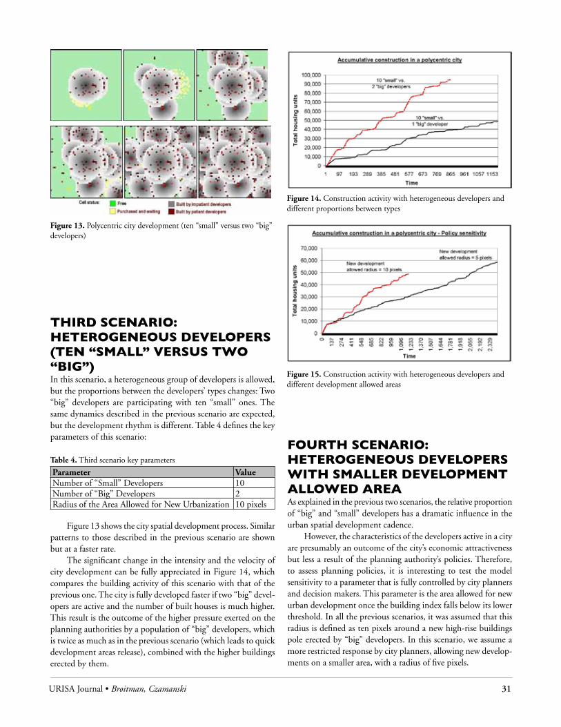
URISA Journal • Broitman, Czamanski 31
thIRd ScEnARIo: hEtERoGEnEoUS dEvEloPERS (tEn “SMAll” vERSUS two “BIG”)In this scenario, a heterogeneous group of developers is allowed, but the proportions between the developers’ types changes: Two “big” developers are participating with ten “small” ones. The same dynamics described in the previous scenario are expected, but the development rhythm is different. Table 4 defines the key parameters of this scenario:
Table 4. Third scenario key parameters
Parameter ValueNumber of “Small” Developers 10Number of “Big” Developers 2Radius of the Area Allowed for New Urbanization 10 pixels
Figure 13 shows the city spatial development process. Similar patterns to those described in the previous scenario are shown but at a faster rate.
The significant change in the intensity and the velocity of city development can be fully appreciated in Figure 14, which compares the building activity of this scenario with that of the previous one. The city is fully developed faster if two “big” devel-opers are active and the number of built houses is much higher. This result is the outcome of the higher pressure exerted on the planning authorities by a population of “big” developers, which is twice as much as in the previous scenario (which leads to quick development areas release), combined with the higher buildings erected by them.
foURth ScEnARIo: hEtERoGEnEoUS dEvEloPERS wIth SMAllER dEvEloPMEnt AllowEd AREAAs explained in the previous two scenarios, the relative proportion of “big” and “small” developers has a dramatic influence in the urban spatial development cadence.
However, the characteristics of the developers active in a city are presumably an outcome of the city’s economic attractiveness but less a result of the planning authority’s policies. Therefore, to assess planning policies, it is interesting to test the model sensitivity to a parameter that is fully controlled by city planners and decision makers. This parameter is the area allowed for new urban development once the building index falls below its lower threshold. In all the previous scenarios, it was assumed that this radius is defined as ten pixels around a new high-rise buildings pole erected by “big” developers. In this scenario, we assume a more restricted response by city planners, allowing new develop-ments on a smaller area, with a radius of five pixels.
Figure 13. Polycentric city development (ten “small” versus two “big” developers)
Figure 14. Construction activity with heterogeneous developers and different proportions between types
Figure 15. Construction activity with heterogeneous developers and different development allowed areas

32 URISA Journal • Vol. 24, No. 1 • 2012
Table 5 defines the key parameters of this scenario:
Table 5. Fourth scenario key parameters
Parameter ValueNumber of “Small” Developers 10Number of “Big” Developers 1Radius of the Area Allowed for New Urbanization 5 pixels
Obviously, because new development areas are smaller, the spatial development process is slower compared with the case of a ten-pixel radius. The following graph in Figure 15 shows the difference between both policy options.
Another important difference between those two policy op-tions is that the development intensity of the city is higher when the allowed area is smaller. Because developers’ time impatience is fixed, smaller allowed areas imply that impatient developers will build higher buildings to maximize profits. Although “big” developers’ behavior does not change under different city policies, changes in “small” developers’ behavior are enough to provoke an overall more intense development. Figures 16 and 17 show the final city configuration and the heights distribution for the case of a development radius of five pixels.
dIScUSSIonThe basic, traditional urban economic models (Alonso 1964, Mills 1967, Muth 1969) are powerful tools able to explain the main forces behind cities’ development. However, their spatial outcomes assume the form of a well-organized monocentric city, a pattern that is hardly verified in any modern city (Irwin and Bockstael 1998, Wha et al. 2011, Serra and Pinho 2011). Several efforts were invested enriching the basic model to explain sprawl and scattered development, for example, assuming landowners intertemporal planning (Mills 1981), perfect foresight of land rent value (Wheaton 1982, Fujita 1982), or dynamic residential
processes (Turnbull 1988). In most of those models, municipali-ties’ regulation roles and planning policies are neglected or at least assumed to have little influence. We claim that the combination between urban planning policies and developers’ behavior can explain much of the city spatial development patterns. In previ-ous papers, the influence of the characteristic time imposed by planning authorities on leapfrogging dynamics in linear spaces was analyzed in a single city model (Czamanski and Roth 2011) and assuming two interacting municipalities (Czamanski and Broitman 2011). In this paper, our objective is to explore the assumption that different types of developers exist (“big” and “small,” characterized by scale of operations, availability of own capital, and time preferences), which are differentially affected by city planning policies expressed as spatial characteristic time settings, and some of them are able, in turn, to influence those policies.
There is growing evidence that urban development can be considered a complex system (Wilson 2006) with self-organizing characteristics (Kumar et al. 2007). Moreover, some scholars claim that cities and networks of cities may represent cases of self-organizing criticality (Batty and Xie 1999, Chen and Zhou 2008). The insights that our model can reveal exploring such issues are beyond the scope of the present paper, but they seem promising and, therefore, we suggest them as possible futures lines of research.
conclUSIonSWhile traditional urban models cannot explain the formation of polycentric urban development patterns, here we explain it by analyzing the interaction between real estate developers’ choices and municipal planning policies. While planning policies differ among countries, in many places zoning variances are possible. Our model indicates phase transitions in the urban spatial con-figuration as a result of the behavior of homogenous “small”
Figure 16. Final stage of a polycentric city development with development radius = five
Figure 17. Heights from above in a city with
development radius = five. Bright gray pixels represent
low-rise buildings (less than ten stories), gray
pixels medium-rise buildings (11 to 30), and
black pixels high-rise buildings (more than 31
floors)

URISA Journal • Broitman, Czamanski 33
developers or a mix of “small” and “big” developers. Sprawling suburbs, scattered land development, and subcenters emergence follows the complex dynamics created by “big” and “small” de-velopers’ choices in time and space. These results shed light on possible outcomes of planning policies, in particular outcomes of restrictive development policies that at times become coun-terproductive. The resemblance between the spatial dynamics resulting from our model and self-organizing criticality models’ outcomes suggests that further research on linkages between them is promising.
Acknowledgements
“The authors wish to thank to the Israel Science Foundation (grant number 666/10) and the Technion - Lower Saxony Re-search Fund for partial funding.”
About the Authors
Corresponding Address:Daniel CzamanskiFaculty of ArchitectureTechnion—Israel Institute of Technology Haifa 32000 Israel [email protected]
The authors are associated with ComplexCity Research Lab Faculty of Architecture and Town Planning Technion - Israel Institute of Technology“
References
Alonso, W. 1964. Location and land use. Cambridge: Harvard University Press.
Alperovich, G., and J. Deutsch. 2000. Urban non-residential density functions: Testing for the appropriateness of the exponential function using a generalized box-cox transfor-mation function. Annals of Regional Science 34: 553-68.
Batty M., and Y. Xie. 1999. Self-organized criticality and urban development. Discrete Dynamics in Nature and Society 3: 109-24.
Benguigui L., D. Czamanski, and M. Marinov. 2001a. The dynamics of urban morphology: The case of Petah Tikvah. Environment and Planning B 28: 447-60.
Benguigui, L., D. Czamanski, and M. Marinov. 2001b. City growth as a leap-frogging process: An application to the Tel Aviv metropolis. Urban Studies 38(10): 1819-39.
Benguigui, L., and D. Czamanski. 2004a. Simulation analysis of the fractality of cities. Geographical Analysis 36(1): 69-84.
Benguigui, L., D. Czamanski, and M. Marinov. 2004b. Scaling and urban growth. Journal of Modern Physics C 15(7): 989-96.
Benguigui, L., E. Blumenfeld, and D. Czamanski. 2006. The dynamics of urban morphology. Environment and Planning B 33: 269-84.
Chen, Y., and Y. Zhou. 2008. Scaling laws and indications of self-organized criticality in urban systems. Chaos, Solitons and Fractals 35: 85-98.
Czamanski, D., and D. Broitman. 2011. Developers’ choices under varying characteristic time and competition among municipalities. Forthcoming in Annals of Regional Science.
Czamanski, D., and R. Roth. 2011. Characteristic time, develop-ers’ behavior and leapfrogging dynamics of high-rise build-ings. Annals of Regional Science 46(1): 101-18.
Fujita, M. 1982. Spatial patterns of residential development. Journal of Urban Economics 12: 22-52.
Fujita, M. 1989. Urban economic theory, land use and city size. Cambridge: Cambridge University Press.
Furst C., M. Volk, K. Pietzsch, and F. Makeschin. 2010. Pimp your landscape: A tool for qualitative evaluation of the ef-fects of regional planning measures on ecosystem services. Environmental Management 46: 953-68.
Golan, E. 2009. 3D urban morphology. M.A. Thesis, Technion—Israel Institute of Technology.
Henderson, J. V., and A. J. Venables. 2008. The dynamics of city formation. Review of Economic Dynamics doi: 10.1016/j.red.2008.06.003.
Irwin, E. G., and N. E. Bockstael. 1998. Endogenous spatial externalities: Empirical evidence and implications for the evolution of exurban residential land use patterns. In Anselin and Florax, Eds. Advances in spatial econometrics.
Kumar M., W. M. Bowen, and M. Kaufman. 2007. Urban spatial pattern as self-organizing system: An empirical evaluation of firm location decisions in Cleveland–Akron PMSA, Ohio. Annals of Regional Science 41: 297-314.
Lai, S. K., C. Ding, P. C. Tsai, I. C. Lan, M. Xue, C. P. Chiu, and L. G. Wang. 2008. A game-theoretic approach to urban land development in China. Environment and Planning B 35: 847-62.
Mills, E. S. 1967. An aggregative model of resource allocation in a metropolitan area. American Economic Review 57: 197-210.
Mills, E. S. 1981. Growth, speculation and sprawl in a monocen-tric city. Journal of Urban Economics 10: 201-26.
Muth, R. 1969. Cities and housing. Chicago: University of Chicago Press.
Serra, M., and P. Pinho. 2011. Dynamics of periurban spatial structures: Investigating differentiated patterns of change on Oporto’s urban fringe. Environment and Planning B 38: 359-82.
Turnbull, G. K. 1998. Residential development in an open city. Regional Science and Urban Economics 18: 307-20.
Wheaton, W. C. 1982. Urban residential growth under perfect foresight. Journal of Urban Economics 12: 1-21.
Wilson, A. G. 2006. Ecological and urban systems models: Some explorations of similarities in the context of complexity theory. Environment and Planning A 38: 633-46.

URISA Journal • Kocabas, Dragicevic, McCann 35
Integration of a GIS-Bayesian network Agent-based Model in a Planning Support System as framework for Policy
Generation
Verda Kocabas, Suzana Dragicevic, and Eugene McCann
Abstract: The link between theoretical complexity-based land-use models, more particularly agent-based models, and practi-cal planning support systems (PSS) is not yet fully elaborated in the current literature. Land-use models that use agent-based approaches still need to be improved and robustly tested if they are to be used effectively as a component of PSS. The objective of this study is to propose a framework for the integration of agent-based models in PSS to simulate future land use and, thus, influence land-use policy and decision making. To achieve this end, a Bayesian Network–based Agent System (BNAS) model of urban land-use change has been integrated into a PSS. The model incorporates a geographic information system (GIS), Bayes-ian Networks (BNs), and agents that represent locational choice behavior of households and commercial firms. In testing the proposed agent-PSS framework for policy generation, this study uses three land-use change scenarios, each associated with dif-ferent policies for urban development. The framework has been applied to simulations of land-use change in the city of Surrey, British Columbia. The results indicate that the BNAS model can be a useful practical tool to assist urban land-use planners in the examination of ‘what-if ’ scenarios about land-use polices. It can shape the scope and character of decision making and future urban development.
IntRodUctIonPlanning support systems (PSS) are information systems that support planning through problem diagnosis, data collection, mining, spatial and temporal analysis, data modeling, visualiza-tion, scenario building and projection, and collaborative decision making (Saarloos et al. 2008). PSS involve a wide range of tools that are as diverse as the steps of the planning process itself, from data selection and integration to public participation and negotia-tion to final policy compromises and implementation monitoring. There are a variety of models integrated within PSS:
Models that are based on geographic information systems (GIS) and spatial statistics. Some examples of GIS-based mod-els used as PSS are: A “What-if system” (Klosterman 1999), the Planning System for Sustainable Development (PSSD) (Hansen 2001), the System for Planning and Research in Towns and Cit-ies for Urban Sustainability (SPARTACUS) (Lautso 2002), and the Population and Land Use Model (PLUM) (WhatIf? 2011).
Models, such as cellular automata and agent-based models (ABMs), that address the spatiotemporal context of the land-use processes through complexity theory and GIS. Linking PSS with complex system models that are capable of handling the complex spatial and temporal dynamics of urban land-use change will increase their utility as tools for urban and land-use planners’ decision making and policy evaluation (Torrens 2002, Zellner 2008). Complex system models, based on cellular automata or agent-based approaches, allow the generation of different land-use change scenarios and, therefore, facilitate the assessment and the
implications of those scenarios. In PSS, ABMs are models that allow planners to visualize, analyze, and simulate dynamic phenomena emerging from the interaction of individual agents (Saarloos et al. 2008). One of the main advantages of ABMs is their ability to represent the complex and nonlinear interactions among individ-uals and actors that directly influence land-use change. PSS with ABMs make use of dynamic models that combine spatial processes and human decision making (Parker et al. 2003, Benenson 2004).
Saarloos et al. (2005) have developed a multiagent model for generating alternative land-use plans in which the agents are land-use experts who initiate the development of plan proposals and communicate with each other over time to draw up the proposals incrementally. Li and Liu (2008) have utilized an ABM as a spatial exploratory tool for generating alternative development patterns with sustainable development strategies. Kii and Doi (2005) have examined the effectiveness of policy measures aimed at achieving a compact city form by developing the MALUT agent-based model. Ligmann-Zielinska and Jankowski (2007) have applied the CommunityViz Policy Simulator to generate development scenarios to evaluate ABM’s operational use in applied plan-ning settings. Furthermore, Ligmann-Zielinska and Jankowski (2009) have experimented with a utility-based approach and an agent-based model to test different conceptions of risk-explicit decision making. The benefits and drawbacks of the integration of an agent-based model of land-use change and a groundwater flow numerical model have been explored by Zellner and Reeves (2010). They examined the multidimensional effects of land-use

36 URISA Journal • Vol. 24, No. 1 • 2012
patterns and policy implications. Robinson and Brown (2009) have illustrated the use of a GIS-based ABM, called DEED, to produce results that describe the individual and interaction ef-fects of minimum lot-size zoning and land-acquisition strategies on forest cover. Zellner et al. (2009) have employed an agent-based model to explore how underlying microbehaviors affect the payoffs of regional forested space and of local tax revenue obtained by two neighboring municipalities in a hypothetical exurban area. Although all these studies utilize ABMs for urban planning or urban policy evaluation, they are either theoretical (never implemented in real contexts) or they have not been fully integrated into a PSS framework.
Other studies have identified challenges when existing ABMs are used in urban planning. The first challenge relates to simulat-ing agent behavior and interactions. Most ABMs define agent behavior and interactions with rules (Gimblett et al. 1996, Torrens 2006). Rule definition is a challenge in ABM design because:
The large amount of alternatives from which an agent has to choose causes the model runs to be long, producing computational complexity (e.g., endless loops) and consequently modeling error.
The complexity of internal relationships between variables makes the models as black boxes and most of the methods are not designed to handle the complexity.
Additional studies have used random utility theory and multinomial logit models (MNL) (Waddell 2002, Miller et al. 2004, Torrens and Nara 2007). In these models, the variables directly affect the modeling phenomenon and may not account for indirectly interacting variables (in which variable A affects variable B, which then affects the model output). Indirect variable interaction is important because variables in real-world processes do not only affect each other directly. As a result, it is important to include this characteristic in an urban model for it to be realistic. Fuzzy logic has been used for agent decision rules (Graniero and Robinson 2006), but this approach does not provide inference from observed data (Hassan et al. 2010). This is important for analyzing historical trends in urban systems. Neural networks (NN) also have been used in ABM decision rule design (Collins and Jefferson 1992, Gilbert and Terna 2000), but one drawback is that they do not provide information about the relationships between variables (Mas et al. 2004), including how they affect each other and the model output. Genetic and evolutionary algorithms methods also have been used for rule definition to represent human decision making for the ABMs in the land-use change process (Manson 2006). However, the fitness functions of genetic algorithms do not necessarily provide a single solution but a range of solutions and this becomes a disadvantage for agent reasoning and decision making. This limitation makes the agent decision making a complex process because having more than one solution produces longer simulation runs and endless loops.
The second challenge with existing ABMs is the way in which they incorporate dynamic variables and how the system adapts to changing variables. It is difficult to incorporate dynamic variables in the existing models. Their design is not modular and, there-fore, they do not allow the easy addition of updated variables.
Nonmodularity means variables and their relationships are static and permanent. To add a new variable, the model would have to be recoded and redesigned entirely for on-the-fly changes are not possible. In addition, these models do not handle many dynamic variables in the modeling process. Moreover, there is no change in the relationships between model variables during model iterations as a result of changing conditions.
The third challenge with the existing ABMs is how they deal with uncertainty and limited data about agent behavior. ABMs usually are designed to use historical data for which there may not be adequate quantity and quality. This means the models must rely on assumptions and hypotheses and so uncertainty is introduced into the modeling process. To overcome this prob-lem, a certainty measure can be added to the rules (Batty 2005) by which the rules describe how much a change in the certainty of the inputs will change the certainty of the output. However, uncertainty is not easy to localize; thus, it strongly depends on all the parts of the model.
The Bayesian Network–based Agent System (BNAS) model responds to these aforementioned challenges by integrating Bayes-ian Networks (BNs) and an agent-based model. The BNAS model has been conceptualized, developed, and validated for modeling land-use change by Kocabas (2008) and Kocabas and Dragićević (2006). The main objective of this research study is to examine the capabilities of the BNAS model as a policy generator in a PSS framework. By employing BNs in its design, the BNAS model can use backward inference. This means that it is possible to enter a desired land-use pattern into the model and then use it to generate policies that would create that land-use pattern. The resulting simulations can be used as a laboratory for exploring scenarios for urban land-use change. The BNAS-PSS framework was applied to the rapidly growing city of Surrey, British Columbia. Scenarios of land-use change were developed to reflect various urban policies.
BnAS ModEl dESIGnThe BNAS model combines GIS, BNs, and agents to model complex urban land-use change and the spatial relationships between drivers affecting the change. It consists of the following components:
Agent types: The BNAS model includes household agents and commercial firms that settle in a particular urban area. Four different types of agents (three different household agent types and one commercial firm agent type) decide where to live/locate during the simulation periods. Based on socioeconomic charac-teristics that affect how households evaluate locations, household agents are categorized as high-income (annual income more than C$100,000), middle-income (annual income between C$30,000 and C$100,000), and low-income household agents (annual income less than C$30,000). Census data used in this study provides household income information for the agents.
Framework for agent behavior and interactions: The BNAS model utilizes BNs to generate agent decisions through several model iterations (five years each). Each agent type has its own BN to create actions according to the agent’s objective and

URISA Journal • Kocabas, Dragicevic, McCann 37
the state of the environment. The BN associated with an agent is based on conceptualizing the locational choice of an agent as a graph (i.e., network) of connected nodes and linkages. In the graph, nodes represent important variables that affect locational choice and a link from one node to another represents a depen-dency relationship between corresponding variables. To provide quantitative descriptions of the dependency links, BNs utilize probabilistic relations rather than deterministic expressions. BNs employ conditional probabilities, conditional dependence, and joint probability distribution to tackle the challenges of using certainty measures in rule-based models. Through the learning algorithms of BNs, the BNAS model generates the graph, the links, and the conditional probabilities from existing geospatial data. This provides simplicity in rule definition within the ABMs. As a result, the BNAS model does not have a permanent network structure, variables, or conditional probabilities. Rather, variables, their values, and causal relationships differ, depending on the relevant data and study area.
Prior experience of the study area is not necessary when constructing the agents’ rules. Users are able to input all the data available for the urban system that they are modeling. The BNAS model then will select only related variables that will be used in the model. It also will calculate/learn the relationship between variables in the input data. A basic knowledge of data gathering and a basic urban planning background will be adequate for a planner to use the model. In the BNAS, BNs allow all the model variables to have a clear semantic interpretation (interpreting the graph and the links) and allow the conditional probabilities to be intuitively understandable.
BNs also provide the capability to model indirectly interact-ing variables. For example, in the real world, economic factors such as new mortgage regulations and recent recession might affect demand for housing and might lead to decreasing housing prices. However, demand for housing does not directly affect a house-hold’s decision to buy a new house. Rather, housing prices directly affect the decision. As a result, mortgage regulations and demand for housing are indirectly interacting variables on the locational choices of people buying a house, while the price of house is a directly interacting variable. BNs allow these indirectly interact-ing variables to be captured in the model. Moreover, BNs also have causal reasoning capabilities that provide knowledge about the decision making of the agents. Modeling causal relationships with indirectly interacting variables in a complex phenomenon is not an easy task for rule-based systems.
The BNAS model allows the definition of dynamic vari-ables (time-dependent drivers) at the start of each simulation. This allows relationships between variables to change within the iterations and agents to adapt themselves to the changing conditions. The adaptation is accomplished by BNs recalculating the conditional probabilities of the affected variables. With the changing conditions, the BN model that is being used by each agent changes.
The agents are designed to act based on their self-interests. Therefore, an agent chooses a location that maximizes its utility.
Choosing a location becomes their “preference.” For each agent’s BN, there are also decision and utility nodes. A decision node represents the two decision alternatives “choose this location (stay)” or “not choose this location (search for another location).” A utility node represents the expected utility of each possible outcome of each decision.
Furthermore, agents’ behavior is affected by that of other agents. Therefore, each agent impacts the behavior of the others with respect to where to live. When a household agent makes its decision to stay, the location attribute is updated and the popula-tion density of that location increases and affects the other agents’ decisions. When a commercial agent makes its decision to stay, the location attribute is updated and the commercial density of that location increases.
Agents’ environment: The study area is represented as a digital environment in which agents operate. The two-dimension-al space is structured by census units with irregular spatial tessel-lations represented as GIS layers in the vector data format.
The system of agents’ iterations: The BNAS model is composed of static and variable parts. The static parts, which are specific to the BNAS model, include agent types (two main types, four in total), agents’ field of vision, and a definition of model iterations (five-year). The variable parts, which are specific to and change for each study area, consist of data variables (land-use drivers) defined in the BN of each agent, links describing relationships between variables, conditional probabilities between variables, number of agents per agent type, and the model simula-tion time period (e.g., ten years (two model iterations), 20 years (four model iterations), or 50 years (ten model iterations)). Users design the scenarios and corresponding policies by creating vec-tor spatial data and input that information to the BNAS model. These inputs are used as variables in the BNs in each agent type.
During each model iteration, a number of agents for each agent type enter the urban environment one by one. Popula-tion projection data is used to define the total number of agents that enter for each year, corresponding to each time step of the model simulations. The total increase in population for each year (entered by the user) is distributed among different types of agents based on the current distributions of each income group in the population. The numbers can be between 100 agents to one million agents per agent type for each iteration. The agent type entering the simulation is randomly selected by the model.
Each agent can have one of two possible states: It is either searching for or has found a location. A random location is in-itially assigned to each agent together with its own socioeconomic characteristics. With this information, each agent’s BN structure is used to create real-time decisions about a location, that is, the agent who is to make the decision runs the BN model and, based on the result, it makes a decision. If the decision is not to choose one particular location, then the agent searches within a radius of one kilometer (the neighborhood of that particular location) for other possible locations. The search continues until the agent decides on a location. It then stays in that location until the end of the whole simulation.

38 URISA Journal • Vol. 24, No. 1 • 2012
The neighborhood of a spatial unit consists of other spatial units that reside within a radius of one kilometer. The reason behind the radius is to introduce an agent’s field of vision that prevents it from searching the entire urban environment. Each agent has its own characteristics and field of vision and, in combination, they form a heterogeneous agent population in the BNAS model. Thus, agents do not evaluate all possible location alternatives. Instead, they use a sequential choice of local optimizations because rational decisions often are not feasible in ABM and are limited to the finite computational resources. This also is known as bounded rationality (Gigerenzer and Selten 2001). Making agents search the entire city or urban area will lengthen model run-time based on the computer configuration and can make simulations unreasonably long. Each agent type has a different range of vision related to its income level. High-income agents have a wider neighborhood radius to search because they can afford to live in a wider range of neighborhoods.
The next step in the simulation is implemented based on the decision output from the agents. The urban environment changes according to the agents’ decisions at each model iteration as the population densities are calculated after each agent makes its decision on whether to stay in a location or move elsewhere. More than one agent can occupy a spatial unit, again representing real-world situations such as the existence of multifamily housing or a multibusiness commercial complex. However, there is a max-imum limit on the population that can be accommodated in each spatial unit. These limits are conditioned by the residential and commercial density constraints defined by each growth scenario and can change depending on the study area and growth scenarios.
If a location is filled to the maximum capacity, it is no longer
available to other agents who are searching for this location. After all the agents have made their decisions, population density values are updated according to the decisions and, consequently, future land-use patterns are obtained. Thus, the final result of the simulation is the generation of population numbers and densities per census unit. When new commercial firms choose locations in the environment, model variables that are related to employment also are updated. In this way, firms affect each other as well as households and, similarly, households affect each other as well as firms.
Given that the BNAS model is a dynamic model, the system runs each iteration 100 times. It then calculates the average population number and generates final population numbers and densities for each spatial unit. After obtaining these data, the BNAS model generates commercial and residential land-use classes. Residential land-use classes are categorized by densities ranging from high-density to low-density residential (urban) areas. This final land-use information is then used as an input to the next iteration. At the end of the simulation, the BNAS model generates the population densities and land use for each spatial unit. If a spatial unit has no population or commercial usage in the initial year and if it has a population density and/or commercial use at the end of the simulation, that means new development has occurred in that area.
The BNAS model does not define permanent data variables (such as land-use drivers). This means it does not use the same variables, the same relationships between the variables, and the same conditional probabilities for different areas unlike existing ABMs. As a result, the BNAS model variables, the relationships between the variables, and the conditional probabilities change
Figure 1. The link between the planning process and the BNAS model–based planning support system

URISA Journal • Kocabas, Dragicevic, McCann 39
dynamically at the beginning of each simulation depending on the study area, the users’ opinions regarding the variables, and the historical land-use and census data. The use of BNs provides improvement over rules-based systems (Heckerman and Wellman 1995) by allowing BNAS the ability to model even with missing input data. This BNAS model flexibility makes it suitable to be applied in the context of the planning support systems and in different study areas.
MEthodoloGy In this study, the utility of the BNAS model in a PSS framework is tested by using it as a policy generator and a future land-use simulator. When users enter their desired future land-use pat-terns, the BNAS identifies the necessary policies that achieve that future. This is accomplished by BNs’ ability to use both forward and backward inference. This is significant to policy makers for the model provides information about land-use variable interac-tions and how they relate to the locational choices of agents. The following sections describe the novel approach of BNAS in the integration of ABMs as a part of PSS with the application to a real-world city in Canada.
The BNAS Model in a PSS FrameworkA PSS is established after a specific planning problem is identified such as one related to planning for new urban development. Its goals and objectives are identified accordingly. Figure 1 illustrates the components of a PSS, its relation to the planning process, and how a Bayesian Network–based Agent System (BNAS) model fits within this context. The BNAS model can be employed in
a PSS framework for processing information. The next sections explain how an ABM such as the BNAS can be engaged in a PSS framework following the steps presented in Figure 1.
Processing Information from DataAn understanding of land-use change drivers and their interac-tion with each other is of central importance in the analysis and forecasting of land-use change. This study assumes that the micro-level location decisions of households are an important element of land-use change processes. Macroscale drivers that operate from the top down and microscale drivers that work from the bottom up are used as factors that affect agent decision making. The BNAS model can incorporate land-use decisions through the links between the various drivers. With specific BN structures, the causal relationships between drivers are represented in the model. After the potential land-use drivers are defined, the BN structure learning algorithms are executed with different configurations of drivers. By comparing the different BN structures, the important drivers affecting one or more variables in the structure can be used in the agents’ locational decision making.
Figure 2 provides examples of BN structures for the house-hold agents to illustrate how a BN in an agent type can be represented (these are examples and do not represent the BNAS model’s variables). Each node in the network corresponds to a variable that affects an agent’s decision. When an agent is search-ing for a location, the values of each node for that location are entered. The BNAS model then calculates the probabilities for the “choice” node, which represent an agent’s decision to choose a particular location. The links between the nodes indicate how the relationships between them are structured. These links are
Figure 2. Examples of Bayesian Network structures with some land-use drivers as nodes that work on different scales: (a) macroscale BN structure and (b) microscale BN structure
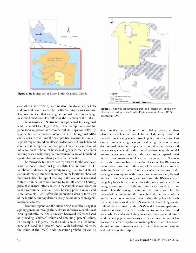
40 URISA Journal • Vol. 24, No. 1 • 2012
established in the BNAS by learning algorithms by which the links and probabilities are learned by the BNAS using the user’s inputs. The links indicate that a change in one will result in a change in all the linked variables, following the direction of the links.
The macroscale BN structure is represented for a regional land-use model (see Figure 2 (a)). The example accounts for population migration and commercial start-ups controlled by regional factors (attractiveness/constraints). The regional ABM can be constructed using the example BN structure to simulate regional migration and the allocation decisions of households and commercial enterprises. For example, climate has some level of influence on the choice of household agents, crime rate affects housing costs, and housing exerts certain influence on household agents’ decisions about their places of settlement.
The microscale BN structure is represented for the local-scale land-use model (shown in Figure 2 (b)). The link from “LRT” to “choice” indicates that proximity to a light rail transit (LRT) station ultimately can have an impact on the locational choice of the households. The type of dwelling in the location is associated with the number of rooms, leading to an influence on housing prices that, in turn, affect choice. In the example shown, closeness to the recreational facilities (Rec), housing prices (Value), and rental amounts (Rent) affect the population density (Density) of the location, but population density has no impact on agents’ locational choices.
This study expands on the initial BNAS model by using it as a policy generator through the backward inference capabilities of BNs. Specifically, the BN is run with backward inference based on providing “children” values and obtaining “parent” values. For example, in Figure 2 (b), the node “choice” is a “children” node and “road” is a “parent” node. With backward inference, the values of the “road” node (posterior probability) can be
determined given the “choice” node. Policy makers or urban planners can define the possible future of the study region and then the model can generate possible policy interventions. This can help in generating ideas and facilitating discussion among decision makers and urban planners about different policies and their consequences. With the desired land-use map, the model assigns the necessary policies to the locations (i.e., spatial units) in the urban environment. Then, each agent runs a BN associ-ated with it, starting from the random location. The BN runs in the opposite direction. In this case, all the variables are known, including “choice,” but the “policy” variable is unknown. In the policy generator option of the model, agents are randomly located in the environment and only one agent runs the BN to calculate the policy for each spatial unit. Once the policy is obtained from the agent running the BN, the agent stops searching the environ-ment. Then, the next agent enters into the simulation. Thus, by the end of the simulation, the model finds the necessary policies for the desired outcomes and then updates the policies for each spatial unit to be used in the BN structures of searching agents. It should be reiterated that the BNAS model has two capabilities. First, it has forward inference capabilities to simulate future land use in which variables including policies are the inputs and future land use and population density are the outputs. Second, it has backward inference capabilities to find policies that will generate desired land-use outcomes in which desired land use is the input and policies are the outputs.
Figure 3. Study area: city of Surrey, British Columbia, Canada
Figure 4. “Growth concentration area” and “green zone” in the city of Surrey according to the Livable Region Strategic Plan (LRSP), adopted in 1996

URISA Journal • Kocabas, Dragicevic, McCann 41
IMPlEMEntAtIon of thE BnAS ModEl In A PSS fRAMEwoRk wIth GRowth ScEnARIoSStudy Area: City of SurreyMetro Vancouver is the third largest urban region in Canada, encompassing 22 municipalities and one electoral area in southwest British Columbia (see Figure 3) with a population of approximately 2.1 million (Statistics-Canada 2011). The region has undergone rapid population growth over the past 30 years. Regional growth has resulted in debates over land-use priorities. In 2002, regional-planning authorities launched the Sustainable Region Initiative, aimed at encouraging social, economic, and environmental sustainability. This initiative builds on the Livable Region Strategic Plan (LRSP), adopted in 1996 (MetroVancou-ver 2011). The LRSP limits growth in a “growth concentration area” and a “green zone,” which consists of the farmland in the Agricultural Land Reserve (ALR), publicly owned parkland, environmentally sensitive areas protected by federal, provincial, or municipal regulation, and other lands identified by individual municipalities (shown in Figure 4).
Drivers of Land-use Change as BNAS Model VariablesThe variables used in the BNAS model application for the city of Surrey are as follows: • Population density (density) is used as a variable for it
is a key factor in land-use change (Hu and Lo 2007). The population variables were obtained from Canada Census data and population density was calculated for each census unit. Population density is grouped into three classes: low (less than 20 people/ha), medium (between 20 and 60 people/ha), and high (more than 60 people/ha).
• Accessibility to major transportation routes—to roads (road) and SkyTrain elevated light rail stations (sky) are used as variables to incorporate the effects of the road network and public transit on land-use change. Accessibility is calculated as the Euclidean distance to the nearest road and light rail stations from the census unit.
• Accessibility to town centers (town) determines residential location in this study. These centers provide a range of retail and office uses, employment, entertainment, cultural and educational services and facilities, and residential housing (see Figure 5). The distance from each town center to the center of each census unit was calculated and the minimum distance for each unit was selected for the nearest town center, such as Guildford, Fleetwood, Newton, Cloverdale and South Surrey centers.
• Distance to employment centers (emp) is taken into account by using a cost-distance function. Cost distance is the calculation of distance in terms of the measure of cost from residential areas to employment centers. Cost distance was used instead of a linear-distance calculation because
any travel to the employment centers incurs costs, either in money, time, or effort. Thus, this cost affects the agents’ locational choice.
• Distances to recreational areas (rec), type of dwellings (type), and number of rooms (rooms) also were used as variables. Housing characteristics were obtained from Canada Census data. Distance to recreational areas was calculated as a Euclidean distance to recreational areas.
• Land prices (value) and rental amounts (rent) affect household locational choices. These variables were obtained from the Canadian Statistics Agency.
• Policy (poly) variable provides different policy options, including taxes, residential density, construction, and land-use constraints/zoning. Each of the policy options and their levels are defined in the policy variable. This allows the BNAS model to generate different growth scenarios. Each scenario has different policy options as presented in Table 1.
Data for major roads and SkyTrain stations were obtained from the Greater Vancouver Transportation Authority (Translink). Town and employment centers data were obtained from Metro Vancouver. The city of Surrey was chosen as a study area because its community plan addresses its dynamic growth in the context of the LRSP (City of Surrey 1996). The vector GIS land-use data for year 2001 was obtained from Metro Vancouver and used as the initial environment for the agents.
The BNAS Simulation Modeling for Planning ScenariosPlanning and growth management in Surrey are dominated by local and regional policies. At the regional level, the city has a growth management framework that is linked to Metro Vancouver’s LRSP. This study’s aim is to compare the BNAS model simulation outcomes with those presented by the LRSP management policies and Surrey’s land-use plan (see Figure 6). For each scenario, the policy variable uses some of the policies defined by LRSP. The PSS framework uses scenarios to generate different policy outcomes. Only growth scenarios (as opposed to stasis or decline scenarios) have been considered because Surrey has adopted a growth man-agement framework and it is a city that is growing continuously.
The urban development scenarios used in this study are a Compact Growth Scenario, an Environmental Growth Scenario, and a Sustainable Growth Scenario. Translating these scenarios into model inputs was accomplished by interpreting policies and creating input files for the model that represents these policy in-terpretations (see Table 1). Although the scenarios have common policies, the level of policy intervention changes depending on the scenario. For example, the Compact Growth Scenario has high tax values for development on previously undeveloped areas. In contrast, the Environmental Growth Scenario is characterized by lower taxes on similar development.
Each scenario has different policy details that have been incorporated in the BNAS model as policy variables. In the Sus-

42 URISA Journal • Vol. 24, No. 1 • 2012
tainable Growth Scenario, low taxes were applied to existing urban areas and high taxes were applied to natural areas. Zoning controls and residential density constraints have been introduced in the policy variable. These policies are examples for the chosen study area but there is no limitation to the policies that can be defined in the model. Although there are high taxes, agents (households or commercial firms) still might prefer to locate in those areas, thus contributing to the emergence of new land-use patterns. The outcome of an agent’s behavior depends on the BN structure and its generated probabilities.
The Compact Growth Scenario aims to promote growth on already urbanized areas. This scenario examines what would occur if policy makers decided to promote growth in existing urban areas. In the scenario, natural areas are not protected by policy interventions and agents are free to choose locations on natural areas.
The Environmental Growth Scenario aims to protect areas of natural significance and amenity, including parks and recreational and agricultural areas, from future urban development. Therefore, it features more policy interventions, such as high taxes, that aim to protect natural areas. It also promotes infill developments but not in levels as high as in the Compact Growth Scenario.
The Sustainable Growth Scenario promotes both compact and environmental growth. Thus, this scenario is a combination of the
two previous scenarios and matches the principles of the LRSP. Therefore, it gives a high level of importance to both compact growth and environmental protection.
These scenarios are examples of planning initiatives that might be adopted in reference to the particular situation in Surrey. The policies underlying the scenarios can be changed for different study areas and, given the BNAS model’s flexibility, there is no limitation on the choice of the scenarios. The scenarios remain fixed during the simulations.
RESUltSTo examine the long-term consequences of different scenarios with various policy settings, based on the available land-use data, six maps with simulation outcomes depicting land-use change at five-year intervals were generated. The time frame for the simu-lations is from 2001 to 2031 (six iterations). The model inputs and outputs are in GIS vector data format. The algorithm of the BNAS was coded in MATLAB with object-oriented design (Mathworks 2011) by using some of the functions of the Bayes Net Toolbox (Murphy 2001) and the Arc_Mat Toolbox (LeSage and Pace 2004) that were loose-coupled with ArcGIS (ESRI 2011). The developed graphic user interface (GUI) allows the configuration of variables, simulation runs, visualization, and
Figure 5. City and town centers in the study area Figure 6. Development map proposed by the Surrey City Community Plan

URISA Journal • Kocabas, Dragicevic, McCann 43
analysis of the BNAS model simulations for the urban land-use data representing the agents’ environment.
The BNAS Model Graphic User InterfaceFigure 7 is a screenshot of the menus in the BNAS model’s GUI. Before running the model, users must configure the model param-eters. Under the BN configuration menu, the user sets up three parameters: Node, Structure, and Conditional Probability Table.
In the Node Configuration menu (see Figure 7 (a)), the user can choose variables and their sizes. This allows the model to be run with different numbers of variables, thus allowing “what-if ” type simulations. Nodes represent variables. The Structure Con-figuration menu has two options (shown in Figure 7 (b)): The user can input a user-created network structure file or the model can learn the network structure from observed data (this option provides ease of use). Moreover, users enter the number of agents to be entered to the simulations for each agent type in a text file. For example, there are four agent types defined by the user cor-
responding to each agent type (three household agents type and one commercial firm type). Conditional probability tables also are learned from the data. Therefore, users only need to define the sample size to be chosen from the training data.
The resultant BN structure (learned from the data) for each agent type is displayed by the GUI as shown in Figure 8. Medium-income and low-income agents’ decisions are affected by the variable describing proximity to town centers. Proximity to recreational areas does not have a direct effect on high-income agents’ decisions according to the learned BN structure. Dwelling types are an important factor for high-income agents’ decisions. Low-income and medium-income agents, on the other hand, have much less choice in their residential decisions and are likely to attach more importance to the availability of rental opportuni-ties. The learned BN structure also suggests that the population density variable does not have a direct effect on the locational choice of the agents.
After the structure of the BN is configured, the next step involves estimating conditional probability table parameters using the CPT Configuration menu (see Figure 7 (c)). To achieve this, the user selects the learn button and the GUI runs the parameter learning algorithm. After the BN is completely set up, the urban environment is created for the agents using the Environment menu (Figure 7 (d)). This is done by reading the ArcGIS shapefile (.shp) for the environment of the study area, finding the neighborhoods for each polygon in the file, and specifying the radius of one kilometer for the neighborhood.
Once these parameters are set, the model is ready to run using the main menu (Figure 7 (e)). Population projection data were obtained from Metro Vancouver (2011) and incorporated for each year corresponding to each time step of the model simulations. This defines the total number of agents used by the BNAS model. In addition, the number of iterations and scenario types are chosen at this stage. There are three available scenarios with different policy settings. The model also allows for the addition of dynamic variables into the simulation through the Dynamic Variables menu (Figure 7 (f )). The user defines which variables are dynamic and at which iteration these variables will be changed. The remaining tasks are implemented within the BNAS model algorithms.
In this example study area, a dynamic variable is defined by adding new roads to the transportation network, which will alter the distance variable in the model. The BN, with each as-sociated agent, recalculates the conditional probabilities of the distance variable. Thus, the BN model now is changed. Agents adapt themselves to the changing conditions by recalculating the conditional probabilities.
The population density map is displayed at the end of each simulation iteration. When the simulation is complete, the final resulting map of land use is displayed on the screen. After a scenario type is chosen, users can display land-use and population maps for each scenario and iteration with options for selecting any iteration and color for the map categories. With the tabular output option, users can compare urban land-use changes with the change graphs and tables.
Table 1. The three urban development scenarios and their associated urban policies
Compact Growth Scenario
• Promoting growth around existing urban areas through tax
• deductions that result in lower land prices and rents
• Applying residential density constraints (ac-cording to the city of Surrey’s goals)
• Land-use zoning controls• Infill development on already urbanized
land• Encouraging new neighborhood centers
Environmental Growth Scenario
• Excluding ALR and green zone from devel-opment
• High taxes on natural areas that result in high land prices and rents
• Land-use controls limiting construction permits
• Infill development on already urbanized land
Sustainable Growth Scenario
• Promoting growth in existing urban areas through tax deductions that result in lower land prices and rents
• Applying residential density constraints (ac-cording to the city of Surrey’s goals)
• Land-use zoning controls• Excluding ALR and green zone from devel-
opment• High taxes on natural areas that result in
high land prices and rents• Limiting construction permits• Infill development on already urbanized
land• Encouraging new neighborhood centers
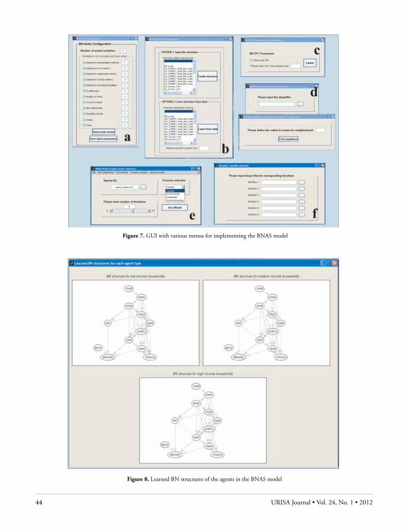
44 URISA Journal • Vol. 24, No. 1 • 2012
Figure 8. Learned BN structures of the agents in the BNAS model
Figure 7. GUI with various menus for implementing the BNAS model

URISA Journal • Kocabas, Dragicevic, McCann 45
Simulation OutcomesCompact Growth Scenario simulation outcomes are presented in Figure 9 with the initial land-use map for the year 2001 Figure 9 (a) and the simulated land-use map for the year 2031 Figure 9 (b). Some of the agricultural areas have been converted to medium-density residential uses that can be identified by visual comparison between maps in Figure 9 (a) and Figure 9 (b). However, new town centers proposed by the Surrey Community Plan (Figure 6) did not emerge in this simulation.
To demonstrate the usefulness of the BNAS model as a part of a PSS in a real-world application with an existing com-munity plan, the system was run as a policy generator to find the necessary policies that would lead to the emerging of new town centers proposed by the Surrey Community Plan at the end of the simulations in 2031. The results from this intermediate run as a policy generator indicate that new employment opportunities should be created around those town centers. Using the Dynamic Variables, new employment opportunities have been added to the mid iterations sequentially, and the model was run with the new policy settings.
Users can create the policy file in the ArcGIS shapefile format. The model uses policy-intervention maps for each scenario in which levels of policies are implemented. For each policy, there is a policy-intervention map that is entered into the system. The figures show a combined policy-intervention map for each sce-nario because of the size limitations of this paper. Because one spatial unit can have more than one policy intervention, the levels show the degree of this intervention in the figures. High levels show more policy interventions, i.e., more than one type of policy intervention. For example, if one spatial unit has high taxes and a limit on construction permits, then the policy-intervention map shows a low level to medium level of policy intervention. If one spatial unit includes all the policy interventions, then the policy intervention map shows high policy intervention. If the spatial unit has only half of the policy interventions, then the map shows medium policy intervention.
Figure 9 (c) summarizes the necessary policy interventions needed in the compact scenario to produce the new town centers that are called for in Surrey’s current community plan. Figure 9 (d) shows the final land-use map after running the model for policy intervention.
A cross-tabulation method is used for comparing the pro-posed and simulated land-use maps. Both vector–GIS format simulation maps were converted to raster format and then com-pared cell by cell to calculate a Kappa index. To calculate a Kappa index, numbers of agreed and nonagreed spatial units were used for they do not change shape between the maps. As a measure of comparison, a Kappa index varies between -1 to 1, where a Kappa index of 1 indicates perfect agreement between two maps. The visual inspection of the maps and a Kappa index of 0.91 indicate that the model predicted most of the land use envisioned by the community plan for the year 2031.
The results also indicate that the compact growth scenario simulated more compact patterns as pointed out by the increase in
the high-density and medium-density residential areas (see Figure 10 (a)). Results show that there are nine times more high-density areas in 2031 than in 2001 under this scenario. In addition, low-density areas decreased by 68 percent and medium-density areas by 60 percent at the end of the simulation period.
Figure 11 presents land use–generated simulations for the Environmental Growth Scenario. Although compact densities were obtained in the existing urban core, agricultural areas, currently under conservation, were seen to attract development. Thus, the BNAS model was run again (i.e., two simulations were run—one with forward inference and one with backward inference) to identify necessary policies to prevent urban expansion on protected areas. The model suggested that an increase in taxes on development in natural areas and more infill development of urban land in the central neighborhood would achieve this goal. The land-use map results are shown in Figure 11 (b). They sug-gest that most of the agricultural areas do not become developed. Results indicate that high-density areas increased seven times and low-density areas decreased by 26 percent in the period from 2001 to 2031 (shown in Figure 10 (b)).
Sustainable Growth Scenario simulations for year 2031 are presented in Figure 12. Lighter yellow areas illustrate low-density urban areas while darker brown represents higher densities. Agri-cultural areas were protected and most of the growth occurred around the existing urban areas. As a policy input, the BNAS model used Surrey’s map of environmentally sensitive areas to create a classification of high sensitivity, medium sensitivity, or low sensitivity. High-density areas show a steep increase (ten times) in size by the end of the simulation. Low-density areas decreased by 45 percent in total and medium-density areas by 53 percent in total during the period from 2001 to 2031 (see Figure 10 (c)).
After analyzing the results, urban planners and policy builders can make necessary decisions. They can formulate policies that lead to their desired future land-use outcomes. For example, if they want to take the compact growth approach, they can ana-lyze the model policy map (see Figure 9 (c)) and use it in their land-use plans.
The overall comparison of the changes in urban areas for all scenario types at the end of simulations for year 2031 is presented in Figure 13. The Environmental Growth Scenario results generate more urban areas than do other growth scenario simulations. The Environmental and Compact Growth Scenario simulations have more high-density areas than do the Sustainable Growth Scenario simulations. Medium-density areas have been decreased in all the scenario outcomes. They have been converted into high-density areas. Low-density urban areas have diminished in all simulation results but to the greatest degree in the Compact Growth Scenario. Furthermore, medium-to-high density areas indicate small in-creases in the Compact and Environmental Growth Scenario results but decreased in sustainable results.
For the purposes of testing the BNAS model, the results were compared with the city of Surrey’s Community Plan map. Most of the future development areas designated by the Community Plan were indeed selected in BNAS model outcomes. However,
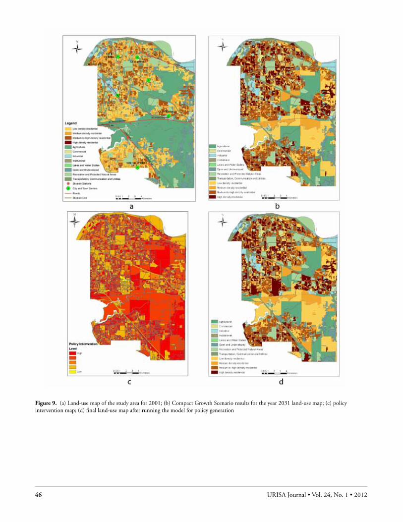
46 URISA Journal • Vol. 24, No. 1 • 2012
Figure 9. (a) Land-use map of the study area for 2001; (b) Compact Growth Scenario results for the year 2031 land-use map; (c) policy intervention map; (d) final land-use map after running the model for policy generation

URISA Journal • Kocabas, Dragicevic, McCann 47
Figure 10. Graph comparing all iterations for (a) Compact Growth Scenario; (b) Environmental Growth Scenario; and (c) Sustainable Growth Scenario

48 URISA Journal • Vol. 24, No. 1 • 2012
Figure 11. (a) Land-use map of the study area for 2001; (b) Environmental Growth Scenario results for the year 2031 land-use map; (c) policy intervention map

URISA Journal • Kocabas, Dragicevic, McCann 49
Figure 12. (a) Land-use map of the study area for 2001; (b) Sustainable Growth Scenario results for the year 2031 land-use map; (c) policy intervention map; (d) final land-use map after running the model for policy generation

50 URISA Journal • Vol. 24, No. 1 • 2012
urban densities change depending on the scenario employed. The South Newton area (Area D in Figure 6) is designated as a new urban neighborhood by the plan, for example. The Environmental and Sustainable Growth Scenarios envision high-density urban development in this area. However, the Compact Growth Scenario generates more high-density neighborhoods in the city center and existing urban areas than in the South Newton area.
The Port Kells area (area A in Figure 6) is defined as hav-ing potential for long-term development by the plan. Only the Sustainable Growth Scenario results show medium-density development in this area while the others generate low density. Grandview Heights (area F in Figure 6) is another area designated as potential growth area on which the Compact Growth Scenario generated a medium-density urban development while the others generate low density. These comparisons indicate how differ-ent scenarios with different policy combinations can affect the locational choices in, and thus the density of, urban areas. Using the BNAS model gives policy makers and urban planners the opportunity to see the consequences of different policy interven-tions. Therefore, the BNAS model should be a part of a PSS for it improves decision-making practices, and it also can be used as a flexible, user-friendly tool for answering “what-if”–type questions.
conclUSIonThe aim of this study is to test the capability of an agent-based model, particularly the BNAS model, to be used as a policy gen-erator within a PSS framework. The model generates dynamic land-use change and was used to apply land-use scenarios that can be explored by urban planners. The BNAS model functionality was tested in real-world situations as a part of a PSS for land-use planning practitioners. The BNAS model uses GIS, Bayesian Networks (BNs), and agent-based approaches incorporated in a PSS framework to simulate future urban growth and urban polices related to the study region. The model relies on BNs to represent complex spatial relationships between numerous land-use drivers that affect urban growth. Agents’ decision making was defined using causal relationships between model variables
in the context of existing and potential future urban policies. The proposed BNAS model as a part of PSS is open to external inputs to simulate the outcomes of alternative policies for each scenario. Because environmental and socioeconomic conditions and related policy goals are location-specific, this study developed a general framework and applied it to a specific, policy-relevant context of the city of Surrey, British Columbia. The simulations were used as laboratories to explore the consequences of different urban policies. The BNAS model represents a spatial and dynamic approach that enables planners to view and analyze the future outcomes of current decisions and policies before they are put into action. It has the ability to help improve planners’ fundamental understanding of the dynamics of land-use change. The results reveal that the BNAS model–based PSS framework can be used as a policy generator—a unique feature that allows users to enter a desired land-use pattern and use it to identify the policy options that are required to achieve the desired land-use pattern.
Comparing the learned structure of the BNAS model with questionnaire surveys is the next step for this work. Further-more, adding significance tests to the simulation results would be beneficial.
Acknowledgments
The authors thank the Natural Sciences and Engineering Research Council (NSERC) and the Social Sciences and Humanities Research Council (SSHRC) of Canada for the financial sup-port of this study. Metro Vancouver and the Greater Vancouver Transportation Authority (Translink) provided some of the spatial data. The MATLAB software was made available by the Network Support Group, Faculty of Applied Sciences, and Cen-ter for Systems Science at Simon Fraser University. The authors appreciate the valuable comments of two anonymous reviewers and the guest editors.
About the Authors
Verda Kocabas has a Ph.D. in geography and is an Alberta Innovates R&D Associate at Blackbridge Geomatics Corporation. Previously, she was a researcher in the Spatial Analysis and Modeling Laboratory, Simon Fraser University, Burnaby, Canada. Her research focuses on geographic infor-mation systems and science, remote sensing, urban planning, and environmental management. She has published in these areas and on developing urban growth models based on cel-lular automata and agent-based approaches.
Corresponding Address: Spatial Analysis and Modeling Laboratory Department of Geography Simon Fraser University 8888 University Drive Burnaby, BC, V5A 1S6, Canada [email protected]
Figure 13. Comparison of the change in each urban density category for all growth scenarios

URISA Journal • Kocabas, Dragicevic, McCann 51
Suzana Dragicevic is a professor in the Department of Geography, Simon Fraser University, Burnaby, Canada. She has acquired more than 20 years of academic experience with geographic information systems and science, with a focus on spatial analysis and modeling. She is conducting an active research program within the Spatial Analysis and Modeling (SAM) Research Laboratory at Simon Fraser University concerning the integration of complexity, GIS, and soft computing for multiscale spatial modeling and decision making. Applica-tions areas include land-use/land-cover change, urban growth, geography, epidemiology, forestry, and landscape ecology.
Corresponding Address: Spatial Analysis and Modeling Laboratory Department of Geography Simon Fraser University 8888 University Drive Burnaby, BC, V5A 1S6, Canada [email protected] Telephone: (778) 782-4621; fax: (778) 782-5841
Eugene McCann is an associate professor in the Department of Geography at Simon Fraser University, Burnaby, Canada. His research addresses urban policy making and urban politics, with a specific interest in the social, economic, and material effects of the circulation of policy models among cities. His specific empirical foci are urban drug policies and urban planning and design policies.
Corresponding Address: Department of Geography Simon Fraser University 8888 University Drive Burnaby, BC, V5A 1S6, Canada [email protected]
References
Batty, M. 2005. Cities and complexity: Understanding cities with cellular automata, agent-based models, and fractals. Cambridge, MA: MIT Press.
Benenson, I. 2004. Agent-based modeling: From individual resi-dential choice to urban residential dynamics. Goodchild, M. F., and D. G. Janelle, Eds. Spatially integrated social science. New York: Oxford University Press, pp. 67-95.
City of Surrey. 1996. Surrey official community plan by-law 12900. Http://www.surrey.ca/bylawsand councillibrary/REG_OCP_12900.pdf, accessed April 22, 2011.
Collins, R. J., and D. R. Jefferson. 1992. Antfarm: Towards simulated evolution. In Langton, C. G., Ed. Artificial Life II: Proceedings of the Workshop on Artificial Life. Redwood City, CA: Addison-Wesley, pp. 579-601.
ESRI. 2011. Http://www.esri.com, accessed April 22, 2011.Gigerenzer, G., and R. Selten. 2001. Bounded rationality the
adaptive toolbox. Cambridge, MA: MIT Press.
Gilbert, N., and P. Terna. 2000. How to build and use agent-based models in social science. Mind and Society 1(1): 57-72.
Gimblett, H. R., B. Durnota, and B. Itami. 1996. Spatially-explicit autonomous agents for modeling recreation use in complex wilderness landscapes. Complexity International 3.
Graniero, P. A., and V. B. Robinson. 2006. A probe mechanism to couple spatially explicit agents and landscape models in an integrated modeling framework. International Journal of Geographic Information Science 20 (9): 965-90.
Hansen, H. 2001. Pssd—Planning system for sustainable de-velopment. The methodical report. Http://www2.dmu.dk/1_viden/2_Publikationer/3_fagrapporter/abstrakter/abs_351_uk.asp, accessed April 22, 2011.
Hassan, S., L. Garmendia, and J. Pavón. 2010. Introducing uncertainty into social simulation: Using fuzzy logic for agent-based modelling. International Journal: Reasoning-based Intelligent Systems 2 (2): 118-24.
Heckerman, D., and M. P. Wellman. 1995. Bayesian networks. Communications of the ACM 38 (3): 27-30.
Hu, Z., and C. P. Lo. 2007. Modeling urban growth in Atlanta using logistic regression. Computers, Environment and Urban Systems 31: 667-88.
Irwin, E. G., and J. Geoghegan. 2001. Theory, data, methods: De-veloping spatially explicit economic models of land use change. Agriculture, Ecosystems and Environment 85 (1-3): 7-24.
Kii, M., and K. Doi. 2005. Multiagent land-use and transport model for the policy evaluation of a compact city. Environ-ment and Planning B - Planning and Design 32(4): 485-504.
Klosterman, R. E. 1999. The what if? colloborative planning sup-port system. Environment and Planning B 26(3): 393-408.
Kocabas, V. 2008. Toward integration of Bayesian networks with geographic information systems and complex systems theory for urban land use change modelling. Burnaby: Simon Fraser University Ph.D. Thesis.
Kocabas, V., and S. Dragićević. 2006. Integrating GIS and Bayes-ian networks for a multi-agent model of land use change. 44th Annual Conference of the URISA Proceedings, Van-couver, Canada, September 26 to 29, http://downloads2.esri.com/campus/uploads/library/pdfs/64836.pdf.
Lautso, K. 2002. The Spartacus system for defining and analysing sustainable urban land use and transport policies. In Geert-man, S., and J. Stillwell, Eds. Planning support systems in practice. Heidelberg: Springer, pp. 453-63.
Lempert, R. 2002. Agent-based modeling as organizational and public policy simulators. Proceedings of the National Academy of Sciences of the United States of America 99 (3): 7195-96.
LeSage, J. P., and R. K. Pace. 2004. Arc_Mat, a Toolbox for using Arcview shape files for spatial econometrics and statistics. Lecture Notes in Computer Science 3234: 179-90.
Li, X., and X. Liu. 2008. Embedding sustainable development strategies in agent-based models for use as a planning tool. International Journal of Geographic Information Science 22(1): 21-45.

52 URISA Journal • Vol. 24, No. 1 • 2012
Ligmann-Zielinska, A. 2009. The impact of risk-taking attitudes on a land use pattern: An agent-based model of residential development. Land Use Science 4(4): 215-32.
Ligmann-Zielinska, A., and P. Jankowski. 2007. Agent-based models as laboratories for spatially explicit planning policies. Environment and Planning B 34(2): 316-35.
Manson, S. M. 2006. Bounded rationality in agent-based models: Experiments with evolutionary programs. International Jour-nal of Geographical Information Science 20(9): 991-1012.
Mas, J. F., H. Puig, J. L. Palacio, and A. Sosa-Lopez. 2004. Model-ling deforestation using GIS and artificial neural networks. Environmental Modelling and Software 19: 461-71.
Mathworks. 2011. Getting Started with MATLAB. Http://www.mathworks.com/access/helpdesk/help/ pdf_doc/matlab/getstart.pdf, accessed April 22, 2011.
MetroVancouver. 2011. Http://www.metrovancouver.org/Pages/default.aspx, accessed April 22, 2011.
Miller, E. J., J. Douglas Hunt, J. E. Abraham, and P. A. Salvini. 2004. Microsimulating urban systems. Computers, Environ-ment and Urban Systems 28(1-2): 9-44.
Murphy, K. 2001. The Bayes Net Toolbox for Matlab. Computing Science and Statistics 33: 331-50.
Parker, D. C., S. M. Manson, M. A. Janssen, M. J. Hoffmann, and P. Deadman. 2003. Multi-agent systems for the simula-tion of land-use and land-cover change: A review. Annuals of the Association of American Geographers 93(2): 314-37.
Robinson, D., and D. G. Brown. 2009. Evaluating the effects of land-use development policies on ex-urban forest cover: An integrated agent-based GIS approach. International Journal of Geographical Information Science 23(9): 1211-32.
Saarloos, D. J. M., T. A. Arentze, A. W. J. Borgers, and H. J. P. Timmermans. 2005. A multiagent model for alternative plan generation. Environment and Planning B - Planning and Design 32(4): 502-22.
Saarloos, D. J. M., T. A. Arentze, A. W. J. Borgers, and H. J. P. Timmermans. 2008. A multi-agent paradigm as structuring principle for planning support systems. Computers, Environ-ment and Urban Systems 32(1): 29-40.
Statistics-Canada. 2011. Http://www.statcan.ca, accessed April 22, 2011.
Torrens, P. M. 2002. Cellular automata and multi-agent systems as planning support tools. In Geertman, S., and J. Stillwell, Eds. Planning support systems in practice. London: Springer-Verlag, pp. 205-22.
Torrens, P. M. 2006. Simulating sprawl. Annals of the Association of American Geographers 96(2): 248-75.
Torrens, P. M., and A. Nara. 2007. Modeling gentrification dy-namics: A hybrid approach. Computers, Environment and Urban Systems 31(3): 337-61.
Waddell, P. 2002. Urbanism—modeling urban development for land use, transportation, and environmental lanning. Journal of the American Planning Association 68(3): 297-314.
WhatIf? 2011. Http://www.whatiftechnologies.com/, accessed April 22, 2011.
Zellner, M. 2008. Embracing complexity and uncertainty: The potential of agent-based modeling for environmental plan-ning and policy. Planning Theory and Practice 9(4): 437-57.
Zellner, M., and H. W. Reeves. 2010. Integrating land-use and groundwater modeling: Opportunities, challenges and implications for policy analysis. International Journal of Operations and Quantitative Management 16(4): 389-414.
Zellner, M. L., S. E. Page, W. Rand, D. G. Brown, D. T. Robinson, J. Nassauer, and B. Low. 2009. The emergence of zoning policy games in exurban jurisdictions: Informing collective action theory. Land Use Policy 26(2): 256-367.
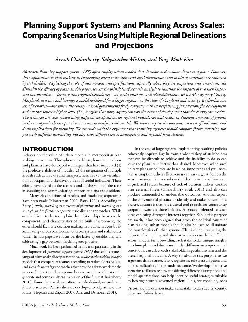
URISA Journal • Chakraborty, Mishra, Kim 53
IntRodUctIonDebates on the value of urban models in metropolitan plan making are not new. Throughout this debate, however, modelers and planners have developed techniques that have improved (1) the predictive abilities of models, (2) the integration of multiple models such as land use and transportation, and (3) the visualiza-tion of outputs and the development of useful indicators. These efforts have added to the toolbox and to the value of the tools in assessing and communicating impacts of plans and decisions.
Many classifications of models and modeling approaches have been made (Klosterman 2000, Batty 1994). According to Batty (1994), modeling as a science of planning and modeling as a strategic tool to further cooperation are distinct approaches. While one is driven to better explain the relationships between the components and characteristics of the built environment, the other should facilitate decision making in a public process by il-luminating various complexities of urban systems and stakeholder values. In this paper, we focus on the latter by establishing and addressing a gap between modeling and practice.
Much work has been performed in this area, particularly in the development of planning support systems (PSS) that can capture a range of plans and policy specifications, multicriteria decision analysis models that compare outcomes according to stakeholders’ values, and scenario planning approaches that provide a framework for the process. In practice, these approaches are used in combination to generate and compare alternative visions of the future (Chakraborty 2010). From these analyses, often a single desired, or preferred, future is selected. Policies then are developed to help achieve that future (Hopkins and Zapata 2007, Avin and Dembner 2001).
Planning Support Systems and Planning Across Scales: comparing Scenarios Using Multiple Regional delineations
and Projections
Arnab Chakraborty, Sabyasachee Mishra, and Yong Wook Kim
Abstract: Planning support systems (PSS) often employ urban models that simulate and evaluate impacts of plans. However, their application to plan making is, challenging when issues transcend local jurisdictions and model assumptions are contested by stakeholders. Neglecting the role of assumptions and specifications, especially when they are important and uncertain, can diminish the efficacy of plans. In this paper, we use the principles of scenario analysis to illustrate the impacts of two such impor-tant considerations—forecasts and regional boundaries—on model outcomes and related decisions. We use Montgomery County, Maryland, as a case and leverage a model developed for a larger region, i.e., the state of Maryland and vicinity. We develop two sets of scenarios—one where the county (a local government) freely competes with its neighboring jurisdictions for development and another where a higher-level (i.e., a regional or state) agency controls the extent of development that the county can receive. The scenarios are constructed using different specifications for regional boundaries and results in different amounts of growth in the county—both rare practices in scenario analysis with models. We then compare the outcomes on a set of indicators and draw implications for planning. We conclude with the argument that planning agencies should compare future scenarios, not just with different desirability, but also with different sets of assumptions and regional formulations.
In the case of large regions, implementing resulting policies coherently requires buy-in from a wide variety of stakeholders that can be difficult to achieve and the inability to do so can leave the plans less effective than desired. Moreover, when such unitary plans or policies are based on important and yet uncer-tain assumptions, their effectiveness can vary a great deal on the actual variations in assumed trends. This limits the achievement of preferred futures because of lack of decision makers’ control over external forces (Chakraborty et al. 2011) and also can produce unintended or undesirable outcomes. Another aspect of the conventional practice to identify and make policies for a preferred future is that it is a useful tool to mobilize community support towards a shared vision. A process oriented to such ideas can bring divergent interests together. While this purpose has merit, it has been argued that given the political nature of plan making, urban models should also be used to illuminate the complexities of urban systems. This includes evaluating the impacts of competing and alternative choices made by different actors1 and, in turn, providing each stakeholder unique insights into how plans and decisions, under different assumptions and conditions, can affect each stakeholder’s specific interests and the overall regional outcome. A way to advance this purpose, as we argue and demonstrate, is to recognize the role of assumptions and other specifications in the model outcome. We develop alternative scenarios to illustrate how considering different assumptions and model specifications can help identify useful strategies suitable to heterogeneously governed regions. This, we conclude, adds
1Actors are the decision makers and stakeholders at city, county, state, and federal levels.

54 URISA Journal • Vol. 24, No. 1 • 2012
value, especially to large regions and planning processes with multiple stakeholders.
Problem Statement: We posit the following:When models attempt to address challenges that transcend ju-risdictional and other boundaries, specifications can limit the outcome of an analysis, sometimes to the detriment of subsequent decisions and plans. Developing and examining scenarios that represent outcomes of different assumptions and specifications can illuminate these limitations and allow identifying and equipping us with necessary strategies for multiple possible futures. Furthermore, identifying and adopting suitable and complementary strategies within the existing fragmented juris-dictional setup can be a better approach for regionally coherent policies than attempting to implement a consensus-based plan for all agencies in the region.
In the next section, we establish the limitations of current ap-proaches to modeling and scenario planning in multistakeholder processes. Then we explain the objective of the paper. In the following section, we discuss our dataset and models and choice of study area. Then we present our analysis and results. We offer some concluding thoughts in the final section.
thE GAP BEtwEEn URBAn ModElInG And PlAnnInG PRActIcE Multiple studies over the years have reviewed and critiqued the role of urban models and PPS in planning practice (see, for ex-ample, Klosterman and Brail 2001, Geertman and Stillwell 2003, Geertman 2006, Hopkins and Zapata 2007). In this section, we establish how they wrestle with the complexities of planning practice in large regions, specifically, those surrounding forecast-ing growth and selecting regional boundaries. We organize the relevant literature into these streams: (1) potential of scenarios to address complexities of plan-making processes; (2) limitations with respect to the use of PPS and (3) their underlying modeling approaches; and (4) spatial planning and the confounding effects of institutional rigidity.
ScEnARIoS, coMPlExIty, And PlAn-MAkInG PRocESSESIn the United States, most urban plans are outcomes of strategic decision-making processes involving multiple actors. Planning processes have attempted to engage these actors through the evalu-ation of alternatives that consider a range of choices, interests, and viewpoints. PSS have provided analytical and visual mechanisms to structure these processes. As a framework, evaluation of alterna-tive outcomes of decisions, i.e., scenario analysis, has been central to the practice of plan making (Chakraborty et al. 2011). From a strategic standpoint, scenario analysis has been used to think about multiple facets of the problem simultaneously and as a tool for addressing the uncertain future in light of the limited cognitive
and computational capacity of individuals and organizations. In particular, it is a tool that fosters imagination as well as critical thinking about how a future might unfold. Since its pioneering application by the RAND Corporation as epitomized by Kahn (1962), it has been used widely in various disciplines ranging from business to military applications (Van der Heijden 1996).
Smith (2007) argued that scenarios can be used in a number of ways and in the regional planning context should be used mostly as a tool for prioritization, oversight, and conversation. Where a participatory paradigm is important, using scenarios as a means of thinking collectively about what to do in different futures should foster thinking of a contingency nature, i.e., if _____, then _____. Neuman (2007) has discussed how scenario planning can encourage planners to dissolve geographic and conceptual boundaries and consider impacts and solutions that extend beyond them. Avin (2007) suggests that scenarios should inform urban plans by creating a platform for public engagement of various groups. Building on earlier work, Avin articulates a 12-step mechanism that includes constructing possible futures as distinct from desired futures. He suggests that these futures with intervention options will provide a framework to evaluate them. Nevertheless, the case studies that follow these prescriptions of the process do not make clear how these interventions are dif-ferent and distinct from the forces that are producing uncertain effects and how one should make plans, given these interactions.
In the practice of metropolitan planning, however, the use of scenario planning has been skewed toward formulating an argu-ment for picking a “preferred future” as opposed to the status quo or business as usual (see, e.g., Council of Fresno County Govern-ments 2009), in direct contrast with the contingency framework of scenario planning. Also, as this review will demonstrate, the participatory framework not only should be capable of compar-ing alternative scenarios, but also should serve other purposes, such as creating plausible alternatives, facilitating questioning institutional rigidities, and creating radical changes in external forces. The PSS used in these approaches also should be able to handle these considerations effectively.
PlAnnInG SUPPoRt SyStEMS And coMPlExItyIn metropolitan planning with its interacting temporal and spatial phenomena, it is almost implausible to think about scenarios with-out resorting to some version of a PSS. Many of these tools offer planners the ability to view complex data, to forecast potential outcomes of decisions and anticipate their implications, and more recently, to communicate these to the wider public. Despite their promise however, PSS have been largely used to—and designed to—facilitate plan evaluation not plan making (Batty 2004).
This disconnect is evident in many of the critiques of PSS. Avin (2007) warns that they should be used only to aid plan-ning processes and to create a platform for engaging with diverse stakeholders, not to define the process. He adds that indetermi-nate factors are the key and those most likely to influence future

URISA Journal • Chakraborty, Mishra, Kim 55
outcomes should be included. Such considerations should be generated through the planning process and multiple sets of variables should be tested. In practice, however, the indeterminate factors often are given less than due consideration and usually are externally specified. For example, the Metropolitan Planning Organizations (MPOs) are required to identify the most likely 25-year growth forecasts within their region, evaluate the impacts on the infrastructure, and then plan for them. The processes often are separated and developing specifications are a precursor to, and not a part of, the planning process. At other times, they are arrived at too rapidly or too early in the process and once estimated they are termed “givens.” The givens then carry through the rest of the process, in effect solidifying and multiplying the potential for error.
Scenarios analysis literature shows us how to tackle this separa-tion and linearity by using the notions of strategic thinking (van der Heijden 2006). For example, Hopkins and Zapata (2007) suggest that planners should move away from the idea of preferred futures and replace it with analysis of possible futures that incorporate more than the most likely future conditions. Such a move can ensure that a wider set of uncontrollable effects and conditions can be consid-ered (e.g., supraregional factors). They admit that such approaches would need planners to make multiple plans. Another aspect of this is balancing increasing technical sophistication of models with the needs of communicating model outcomes in ways that can facilitate decision making. For example, Batty (2004) has argued that the development of most models has been driven by advancement in GIS and remote-sensing technologies but are still only abstractly related to cities as emergent complex systems. Practical applications for planning processes need to be driven by bottom up–driven concerns. As Batty writes, “[T]echnology interacts with policy in diverse, symbiotic ways which develop tensions that get resolved by changes in culture and context as much as by adaptation of the science behind the technology or the technology itself” (p. 329). Thus “good” models are those that can be adequately adapted to the problems at hand in the local or specific context.
Klosterman (2001) reviewed a specific GIS-based PSS called What if? While he notes the utility of PSS for decision makers seeking to broaden and inform public dialogue, he adds that its effectiveness is ultimately limited by the user-specified assump-tion. Similarly, Geertman (2006) has suggested that technology often can outpace planners’ capabilities and framing of prob-lems requiring a dynamic interconnected, with each informing the other in an adaptive utilization, ultimately dependent on a conceptual framework sensitive to context. The above critiques, and there are many others, suggest that it is critical to recognize the capacities and limitations of PSS and, ultimately, choose an approach that captures the important complexities of the context.
lAnd-USE ModElS In PlAnnInG SUPPoRt SyStEMSPSS are often at the interface of underlying models and the deci-sion-making processes. The underlying models are characterized
by their heterogeneity, hierarchical structuring of urban phenom-ena, and approaches to deal with exogenous factors. They can be organized into two broad categories: top-down and bottom-up models. Top-down models employ regression, econometric, and statistical approaches that represent system relationships between aggregate variables depicting best fit of the data. Because of its generalized nature, top-down models are useful for revealing relationships in land-use data and for forecasting purposes. On the other hand, bottom-up models such as agent-based or cel-lular automata models start from a general understanding of the low-level processes and elements, and generate aggregate system behavior by simulating the individual entities in the system.
Top-down models often estimate regional growth projection first and then allocate it among the constituent subgeographies. In the United States, this practice is employed to develop met-ropolitan-level or state-level projections that then are allocated down to the county level and sometimes further down to traffic-analysis zones. Top-down models have been used in management of natural resources (Castella et al. 2007), simulation of system dynamics in multiscalar land-use variables (Veldkamp and Fresco 1996, Brown et al. 2000), and a host of other applications (see Hensher and Button 2004). On the other hand, bottom-up ap-proaches can take top-down outputs as given and look at the spa-tial impacts of them. They also have received significant attention in local-level analysis and decision making (for applications, see Landis 1994, Landis and Zhang 1998, Waddell 2002, Deal and Schunk 2004; for reviews, see Hensher and Button 2004, Kim and Hewings 2011). The choice of a particular model depends on many factors, such as the needs of the project, the availability of data, and user discretion. Still, both kinds are needed to some extent in many planning processes and their insularity can be problematic and deserves careful consideration.
SPAtIAl PlAnnInG And thE confoUndInG EffEct of InStItUtIonAl RIGIdItyFinally, because models attempt to imitate real-world phenomena, they can easily duplicate, and perpetuate, some of its limitations. For example, institutional rigidity, an often-discussed barrier to regional planning (Teitz and Barbour 2007), has become a part of how many models specify and test policies. For example, land-use impacts are often tested last and at a locality level. The high likelihood of these impacts to change as regional policies are changed, and their interdependence with other regional and local forces, often ignored at the local-level analysis. Though these considerations sometimes simplify decision making, they also can limit our anticipation of potential challenges and opportunities.
In addressing these challenges, advancing models alone will not be sufficient. To anticipate adequate variety in future condi-tions and implementation frameworks, planning approaches also will need to encourage and sustain participation. They will have to provide a platform for sharing divergent viewpoints in a pluralistic society and, when combined with evolving tools, help to develop

56 URISA Journal • Vol. 24, No. 1 • 2012
multiple visions for the future that look beyond the traditional limits of scale, time horizon, and disciplinary and institutional boundaries. The literature provides many examples where at-tempts have been made to bridge this gap between empowered advocacy and comprehensive rational planning. It does so most often by utilizing technical tools to empower the stakeholders in the planning process through imagining a normative future (Borjeson et al. 2006, Myers and Kitsuse 2000, Porter 1985). These principles have been used worldwide in many planning processes, including the Norwegian Long Term Program (NLTP), Sustainable Seattle, Oregon Shines, Metropolitan Tunis, and Envision Utah (AtKisson 1996, Barbanente et al. 2002, Grow and Matheson 2006, Kissler 1998).
In addition to unstructured deliberation, several other methods can be applied. One approach sensitive to different stakeholder values is multicriteria decision analysis (MCDA). Malczewski (2006) shows how GIS and MCDA allow diverse (but interdependent) decision makers to insert value judgments and receive feedback on their implications, allowing policy mak-ers to highlight trade-offs between alternatives. Innes and Booher (1999) look at the need for consensus-building planning processes to cope with complex adaptive systems. They suggest that such a framework allows for experimentation, building shared mean-ing, and change.
Still additional considerations may be necessary. For example, metropolitan planning organizations in the United States need to follow a single set of growth projections for transportation planning according to federal requirements for funding. As a result, scenarios (both land use and transportation) have to ac-commodate one set of projections—no more and no less. Unless these requirements change, such agencies have little choice but to use unitary forecasts. They can, however, attempt to consider the wider interactions with other agencies and interdependencies between land use, transportation, and other systems when arriving at their assumptions.
In summary, much has been written about how planning processes use scenario analysis, PSS, and urban models and how their use many be limited by the nature of approaches and insti-tutional consideration, among others. To overcome the resulting challenges, planners will have to balance the sophistication of their tools with accessibility and nimbleness. We argue that some of these challenges can be addressed by systematically considering complexities such as multiple sets of projects and interregional and intraregional interactions, and moving beyond the traditional static definitions of a model region. Scenarios have specific im-plications for plan making and, as we show next, how they are constructed affect the outcomes and subsequent plan-making considerations. Understanding a broader range of uncertainties, as we will show, can allow for better assessment of varying future challenges and as a result can lead to more effective plans.
AnAlytIcAl fRAMEwoRkRESEARch oBjEctIvEIn this paper, we use the principles of scenario analysis to illustrate the impacts of two such important considerations—forecasts and regional boundaries—on model outcomes and related decisions. We use Montgomery County, Maryland, as a case and leverage a model developed for a larger region, i.e., the state of Maryland and vicinity. We develop two sets of scenarios—one where the county (a local government) freely competes with its neighboring jurisdictions for development and another where a higher-level (i.e., a regional or state) agency controls the extent of develop-ment that the county can receive. The scenarios are constructed using different specifications for regional boundaries and result in different amounts of growth in the county, both rare practices in scenario analysis with models. We then compare the outcomes on a set of indicators and draw implications for planning.
dAtA And MEthodSThe models used here have been developed over time by a number of partnering organizations (for details, please see Knaap and Frece 2006, Chakraborty 2010, Mishra et al. 2010, Chakraborty et al. 2011). Our entire modeling area covers the state of Maryland in the United States and some surrounding counties (see Figure 1). One of the purposes of our modeling effort has been to explore alternative futures for the state of Maryland with the intent to identify policies that maximize the likelihood of more desirable future outcomes.
We briefly summarize the modeling framework and method-ology in the following section. The framework is a loosely coupled set of models that work at different scales (national to local), in different areas of specialization, and for different purposes. They interact, however, as shown in Figure 2 and as explained in the following section, and allow us to generate different sets of fore-casts, look at their effect on land-use and transportation networks, and assess their impact using a set of governmental services and quality-of-life indicators. • National econometric model: The national econometric
model consists of two submodels: (1) Long Term Inter-Industry Forecasting Tool (LIFT), a macroeconomic input-output model operating at the U.S. national economy level forecasts more than 800 macroeconomic variables that are then fed into (2) State Employment Modeling System (STEMS) to calculate employment and earnings by industry for all 50 states and the District of Columbia. Output from LIFT serves as input to STEMS. Results from the STEMS model then are allocated by region (political boundaries are imprecise predictors of boundaries of labor markets and economic regions) using current proportions of state-level forecasts for each sector. A detailed description of LIFT and STEMS can be found in the literature (McCarthy 1991, INFORUM 2010).
• Regional model: The regional-level model depicts land-use variables at the county level. At the regional level, the

URISA Journal • Chakraborty, Mishra, Kim 57
forecasting approach is based on a near-total reliance on empirically calibrated relationships. The calibrated model involves 40 equations using progressively more inclusive sets of predictors. The allocation model incorporates review of the benchmark forecasts (Hammer 2007).
• Local model: The local model, titled Landuse Evolution and Impact Assessment Model (LEAM), uses a state-change structured gridded surface whose conditions evolve over time, similar to other cellular automata (CA) technologies (Deal and Pallathucheril 2003).2 The LEAM grid surface is not flat, however, but gains a “hilly” topography based on both physical and socioeconomic constraining factors. It incorporates techniques that calculate a probability to represent the potential of each cell (900 m2 or 0.25 acre) to change from one land-use category to another. This probability of change is influenced by local interactions (e.g., the accessibility of the cell to a predetermined characteristic of its neighborhood or an “attractor”), global interactions (e.g., the state of the regional economy), and other causal mechanisms (e.g., social forces). These produce suitability scores that contribute to the grid surface relief and affect subsequent allocation of development.
2 For more on LEAM, see www.leam.uiuc.edu/maryland.
Figure 2. Loosely coupled modeling framework
Figure 1. Broader region for which model tool has been developed Source: National Center for Smart Growth Research and Education at the University of Maryland

58 URISA Journal • Vol. 24, No. 1 • 2012
Agencies that use models such as those listed previously often work with specific requirements. For example, MPOs use the most likely 25-year employment and household forecasts to test the stresses on travel network. Similarly, local governments updating their land-use plans may use projections from state economic agencies as given to make policies that accommodate that growth or affect it. The purpose of this paper, in part, is to demonstrate that while current approaches are useful for the purposes they serve, additional understanding can be gained by relaxing con-strained projections and testing multiple regional extents.
We specify two scenarios—one where the county (local government) freely competes with neighboring jurisdictions and another where the regional/state government controls the extent of development that the locality can receive. For the first scenario, using our econometric model, we generate county-by-county projections, further detailed into various housing and employment categories using our regional model. For the second, we aggregate county-level projections to the state level. We also specify our land-use models at two scales: one at the level of each county and another at the statewide level.
We selected the case of Montgomery County, Maryland, to demonstrate our point. We could have selected any county for our analysis, but Montgomery County was selected for its rich and
Figure 3. Employment growth Figure 4. Household growth
Table 1. Temporal Development Patterns
Attributes
2010 2030 (2030–2010)Constrained-Development
Competitive-Development
Constrained-Development
Competitive-Development
Constrained-Development Competitive-Development
HH 363,285 357,418 437,464 435,057 74,179 77,639Retail (a) 72,097 72,208 87,268 94,147 15,171 21,939Office (b) 275,831 276,415 333,797 361,792 57,966 85,377Industrial (c) 43,283 43,276 52,391 56,838 9,108 13,562Other (d) 152,268 152,992 184,198 202,266 31,930 49,274Tot. Emp. (a+b+c+d) 543,479 544,891 657,654 715,043 114,175 170,152
varied planning history, its large size, and its high projected growth in the county. To develop the first scenario, we run the land-use model only for Montgomery County and use the projections that are generated for Montgomery County alone, without regard for any interaction with neighboring jurisdictions. We argue that this closely represents a state-imposed growth constraint and call it the Constrained-Development Scenario. For the latter, we use the aggregated state-level projections and run the state-level land-use model. We argue that this represents competing behavior among counties for new growth and call it the Competitive-Development Scenario. This scenario forces competition among municipali-ties for growth without regard to the specific amount of growth projected for each of these jurisdictions by the economic model. From this run, we extract the outcome for Montgomery County and compare it with the stand-alone run for Montgomery County. We compare the outcomes on a few simple indicators. All the models use year 2000 as the base year and are run for every five-year interval, up to 2030.
AnAlySISThe results of model runs are summarized in Table 1. Two sets are household, and employment totals at a county level, for each of the two scenarios, Constraint-Development Scenario and

URISA Journal • Chakraborty, Mishra, Kim 59
Competitive-Development Scenario. These results also were available at a cell level of size 90 m x 90 m. The employment data also is presented by four detail categories—retail, office, industrial, and other. Each scenario run is modeled for two time horizons on year 2000 data: (1) most recent year or 2010 and (2) for the planning horizon 2030. The future year is identified in conformance to the constrained long-range plan for the county and state. The model results show that Montgomery County will receive a higher amount of households and employment in the Competitive-Development Scenario run than in the Constraint-Development Scenario (Table 1). The results suggest that given the flexibility of growth across all counties, and the possibility of moving to a new locality, Montgomery County will attract more households and employment in the Competitive-Development Scenario. This comes at the expense of the counties and happens because of Montgomery County’s higher attractiveness in terms of land-use and accessibility.
The spatial distributions of household and employment growth in these two time periods for both scenarios are shown in Figures 3 and 4, respectively. The polygons in Figure 3 and 4 represent Traffic Analysis Zones (TAZs), showing the numbers estimated from aggregation of the cell-level results.
The new developments in both scenarios for both land-use types happen as expected. The most growth is in areas closer to the urban centers and next to existing modes of transportation. Areas next to transit stations as well as those with a high possibil-ity of redevelopment get a high share of new employment. The overall higher attractiveness and, as a result, the overall higher demand for land, and the location of nearby counties where that new development is getting transferred from can be attributed to the differences seen between the two scenarios.
These differences in total amount and location of new development can be seen in the land-use change indicators. For example, the loss of agriculture and forest land for both model runs are presented in Table 2. As expected, we find the loss to be greater in the Competitive-Development Scenario than in the County-Constraint Scenario. The loss in agriculture and forest land estimation is built into the modeling tools that further uses the land-cover data in the CA-based allocation process. Figure 5 shows the grid-level variations in the scenarios. The grids that are organized according to the amount of new growth received are as follows: (1) higher growth on County-Constraint Scenario, (2) higher growth on the Statewide Scenario, and (3) higher growth under both scenarios. The grid-level results can be used as a tool to visualize differences more specifically.
Table 2. Montgomery County loss of forest and agriculture land (in square meters)
Attribute County Constraint Statewide
Forest Land 36,620,100 62,677,800
Agriculture Land 47,279,700 83,268,000
conclUSIonSFutures are not necessarily given; they also are not necessarily created solely through purposeful action. They are a product of complex interactions of forces that we cannot control as well as decisions we make. Many authors have noted that even the most sophisticated and integrated models are not able to incorporate all variables of interest. Hopkins (2000) explains that numerous urban models have been developed based on different perspectives and theoretical foundations. Some simulate markets for land, housing, and labor, using preferences of households and firms based on past behavior with respect to prices. Still others rely on past probabilities of land conversions and seek an equilibrium solution. Some are dynamic, usually in discrete time intervals in which actions depend on the results of previous time intervals. In this paper, we use a combination of approaches to develop two sets of scenarios—one where a county freely competes with neighboring jurisdictions (Competitive-Development Scenario using a statewide run) and another where the regional/state government controls the extent of development that the locality can receive (Constraint-Development Scenario). The scenarios are constructed using different specifications for regional boundaries and also result in different amounts of growth in the county, both rare practices in scenario analysis with models.
Our analysis has a number of general implications. It shows that assumptions are important and should be carefully chosen. And, if possible, multiple plausible sets of assumptions should be compiled to test the robustness of policies despite variations in assumptions. While similar in concept but different in applica-tion, our study also shows that the choice of regional extents at which models are run affects the outcomes. This is important for a number of reasons. While many studies on limitations of local governance suggest regional coordination as a way to address
Figure 5. Comparison of growth at grid level for both scenarios

60 URISA Journal • Vol. 24, No. 1 • 2012
multiple issues, the scales and composition at which such coor-dination should happen often is unclear. Metropolitan areas often have been used as appropriate scales for most purposes, but with the evolving literature on other scales (for example, watersheds, megaregions, etc.), care should be taken in understanding how these ideas are used in formulating the study region. Or, more importantly perhaps, care should be taken that critical areas are not excluded from the modeled region.
More specifically, our findings suggest that a state-imposed constraint on Montgomery County might be too low in its mag-nitude and thus difficult to implement. It also suggests that in the lack of such constraints, higher amounts of undeveloped lands will be lost resulting in different challenges. The detailed location of development can also be used to argue for or against each set of policies. For example, though it is beyond the scope of this study, it is possible to imagine that a fixed development constraint might be difficult to implement without added political compromise that benefits the county in some ways. The presence of such conditions might complicate the outcome and, indeed, can change the cost/benefit equation for an agency choosing whether to support the constrained or the competitive development policies.
Lastly, the scenario analysis proposed in the paper has prac-tical implications in the state of Maryland. One example is the potential residential and commercial land use for the greater Life Science Center (LSC) proposed in Montgomery County. Based on existing, approved, and proposed development, LSC could yield a maximum of 9,012 additional dwelling units to comple-ment a projected total of 52,500 jobs. The resulting ratio of 5.8 jobs per dwelling unit is based on the existing housing in the greater LSC area (MNCPPC 2010). The Maryland Department of Transportation has concerns that such large-scale development might lead to insufficient transportation infrastructure to sup-port such mixed land-use development. This is an example of the differences between the vision of the county planners and of the state planners for the future of Montgomery County. Such differences, depending on the outcome of a process, can lead to a range of outcomes, two of which have been modeled in the two scenarios presented in this paper. Recognizing these possibilities are important to the planning process.
Another example is Prince George’s County’s Konterra Town Center, a planned mixed-use regional activity center that will include more than 4,500 residential units and more than 5.5 mil-lion square feet of office, retail, and hotel uses to produce more than 10,000 jobs (PGCPD 2009). In contrast to Montgomery County, the state agreed to this development because it supports the construction of the Intercounty Connector (ICC), a major east-west access-controlled highway corridor connecting the two North and South Interstates, 95 and 270. The new development will have access to the ICC and will, in turn, become more at-tractive.
These examples illustrate the kind of decision-making con-flicts and uncertainties that exist between land-use and transpor-tation planning agencies in a large region. Our results show that considering a wider range of possibilities can provide better tools
for those working on these challenges. This includes comparing future scenarios not just with different desirability but with dif-ferent sets of assumptions and regional formulations.
About the Authors
Arnab Chakraborty is an assistant professor in the Department of Urban and Regional Planning at the University of Illinois at Urbana Champaign. His research interests are in land use planning, strategic planning and public participation in plan making. His recent work emphasizes systematic consideration of future uncertainties and linked decisions in the planning process.
611 E. Lorado Taft Drive, M230 Temple Buell Hall (MC-619) Champaign, IL 61821 [email protected]
Sabyasachee Mishra is Research Assistant Professor in the National Center for Smart Growth at University of Mary-land College Park. His research interests focus upon travel demand modeling, transportation planning, travel behavior and transportation economics. His recent work emphasizes on modeling travel demand at statewide and mega regional scale, application of travel behavior principles in transporta-tion decision making.
1112J Preinkert Field House University of Maryland College Park, MD 20740 [email protected]
Yong Wook Kim is a research specialist in the Department of Urban and Regional planning at the University of Illinois at Urbana-Champaign. His research interests focus on the simulation of the urban-sprawl as a decision support tool and data visualization. His recent work emphasizes the use of the information using planning support system, such as the Internet-based portal system.
611 E. Lorado Taft Drive, Temple Buell Hall (MC-619) Champaign, IL 61821 [email protected] Yong Wook Kim Research Programmer Land-use Evolution and Impact Assessment Laboratory University of Illinois at Urbana-Champaign

URISA Journal • Chakraborty, Mishra, Kim 61
References
AtKisson, A. 1996. Developing indicators of sustainable com-munity: Lessons from sustainable Seattle. Environmental Impact Assessment Review 16(4-6): 337-50.
Avin, U. 2007. Using scenarios to make urban plans. In Hopkins, L. D., and M. A. Zapata, Eds. Engaging the future: Using forecasts, scenarios, plans, and projects. Cambridge, MA: Lincoln Institute of Land Policy.
Avin, U. P., and J. L. Dembner. 2001. Getting scenario-building right. Planning November, 2001 22-27.
Barbanente, A., A. Khakee, and M. Puglisi. 2002. Scenario build-ing for metropolitan Tunis. Futures 34(7): 583-96.
Batty, M. 1994. A chronicle of scientific planning: The Anglo-American modeling experience. Journal of the American Planning Association 60(1): 7-16.
Batty, M. 2004. Dissecting the streams of planning history: Technology versus policy through models. Environment and Planning B: Planning and Design 31(3): 326-30.
Börjeson, L., M. Höjer, K. H. Dreborg, T. Ekvall, and G. Finn-veden. 2006. Scenario types and techniques: Towards a user’s guide. Futures 38(7): 723-39.
Brown, D. G., B. C. Pijanowski, and J. D. Duh. 2000. Modeling the relationships between land use and land cover on private lands in the Upper Midwest, USA. Journal of Environmental Management 59(4): 247-63.
Castella, J. C., S. P. Kam, D. D. Quang, P. H. Verburg, and C. T. Hoanh. Combining top-down and bottom-up modelling ap-proaches of land use/cover change to support public policies: Application to sustainable management of natural resources in northern Vietnam. Land Use Policy 24(3): 531-45.
Chakraborty, A. 2010. Scenario planning for effective regional governance: Promises and limitations. State and Local Gov-ernment Review 42(2): 156.
Chakraborty, A., N. Kaza, G. J. Knaap, and B. Deal. 2011. Ro-bust plans and contingent plans. Journal of the American Planning Association 77: 3.
Council of Fresno County Governments. 2009. Request for pro-posal: San Joaquin Valley blueprint roadmap. Http://www.countyofkings.com/kcag/Whats%20New/Blueprint%20Road map%20RFP.pdf.
Deal, B. 2001. Ecological urban dynamics: The convergence of spatial modelling and sustainability. Building Research and Information 29(5): 381-93.
Deal, B., and D. Schunk. 2004. Spatial dynamic modeling and urban land use transformation: A simulation approach to assessing the costs of urban sprawl. Ecological Economics 51(1-2): 79-95.
Geertman S, Stillwell JCH (eds.). 2009. Planning Support Sys-tems Best Practice and New Methods. Springer: New York.
Geertman, S. 2006. Potentials for planning support: A planning-conceptual approach. Environment and Planning B: Plan-ning and Design 33: 863-80.
Grow, R. J., and A. Matheson. 2006. Envision Utah: Laying the foundation for quality development. Urban Land 65(4): 63.
Hammer, T. 2007. Regional forecasting procedure. College Park: National Center for Smart Growth Research and Education Reports, University of Maryland.
Hensher, D. A., and K. Button. 2004. Transport geography and spatial systems. Handbook 5 of the handbook in transport. Kidlington, Oxford: Pergamon/Elsevier Science, pp. 127-46.
Hopkins, L. D., and M. A. Zapata, Eds. 2007. Engaging the Future: Forecasts, scenarios, plans and projects. Cambridge, MA: Lincoln Institute of Land Policy.
Hopkins, L. D., and M. A. Zapata. 2007. Engaging the future: Tools for effective planning processes. In Hopkins, L. D., and M. A. Zapata, Eds. Engaging the future: Using forecasts, scenarios, plans, and projects. Cambridge, MA: Lincoln Institute of Land Policy.
INFORUM. STEMS and LIFT model. 2010. Http://www.inforum.umd.edu/services/models/ stems.html, Accessed January 2011.
Innes, J. E., and D. E. Booher. 1999. Consensus building and complex adaptive systems: A framework for evaluating collaborative planning. Journal of the American Planning Association 65(4): 412-23.
Kahn, H. 1962. Thinking about the unthinkable. Ann Arbor, MI: University of Michigan Press.
Kim JH, Hewings GJD. Framing urban systems and planning concerns as a multi-level problem: A review of the integrated urban system models with an emphasis on their hierarchical structures. In N ancy Brooks, Kieran Donaghy and Gerrit-Jan Knaap (eds.) Oxford University Press Handbook of Urban Economics and Planning. 2010. Oxford.
Kissler, G. R., K. N. Fore, W. S. Jacobson, W. P. Kittredge, and S. L. Stewart. 1998. State strategic planning: Suggestions from the Oregon experience. Public Administration Review 58(4).
Klosterman, R. E., and R. K. Brail, Eds. 2001. Planning support systems: Integrating geographic information systems, models, and visualization tools. Redlands, CA: ESRI Press.
Knaap, G. J., and J. W. Frece. 2006. Smart growth in Maryland: Looking forward and looking back. Idaho Law Review 43: 445.
Landis, J. D. 1994. The California urban futures model: A new generation of metropolitan
simulation models. Environment and Planning B 21: 399-420.Landis JD. Imagining Land Use Futures: Applying the California
Urban Futures Model. Journal of the American Planning Association. 1995;61(4):438–457.
Malczewski, J. 2006. GIS-based multicriteria decision analysis: A survey of the literature. International Journal of Geographical Information Science 20(7): 703-26.
McCarthy, B. M. 1991. LIFT: INFORUM’s model for the U.S. economy. Economics Systems Research 3(1): 15-36.

62 URISA Journal • Vol. 24, No. 1 • 2012
Mishra, S., X. Ye, F. Ducca, and G. Knaap. 2010. A functional integrated land use-transportation model for analyzing transportation impacts in the Maryland–Washington, DC, region. Journal of Sustainability: Science, Practice, and Policy 7(2): 1-10.
MNCPPC. 2010. Greater Seneca science corridor master plan: The Life Sciences Center. The Maryland-National Capital Park and Planning Commission, Web report: http://www.montgomeryplanning.org/community/gaithersburg/docu-ments/GSSCApprovedandAdopted050511web.pdf, accessed May 20, 2011.
Myers, D., and A. Kitsuse. 2000. Constructing the future in planning: A survey of theories and tools. Journal of Planning Education and Research 19: 221-31.
Neuman, M. 2007. How we use planning: Planning cultures and images of futures. In Hopkins, L. D., and M. A. Zapata, Eds. Engaging the future: Using forecasts, scenarios, plans, and projects. Cambridge, MA: Lincoln Institute of Land Policy.
PGCPD. 2009. Prince George’s County biotechnology research and development study. Prepared for the Maryland-National Capital Park and Planning Commission, Web report: http://www.pgplanning.org/Assets/Planning/Countywide+Planning/Research/Biotech+Study+2.pdf, ac-cessed: May 20, 2011.
Porter, DR. Downtown linkages. Urban Land Inst; 1985. Wash-ington D.C.Teitz M, Barbour E. Megaregions in California: challenges to planning and policy. In: The Healdsburg Re-search Seminar on Megaregions.; 2007:7–19.
Van der Heijden, K. 1996. Scenarios: The art of strategic conver-sation. Chichester, UK: John Wiley and Sons.
Veldkamp, A., and L. O. Fresco. 1996. CLUE-CR: An integrated multi-scale model to simulate land use change scenarios in Costa Rica. Ecological Modeling 91(1-3): 231-38.
Waddell, P. 2002. UrbanSim: Modeling urban development for land use, transportation, and environmental planning. Jour-nal of the American Planning Association 68(3): 297-314.

URISA Journal • Steenberghen, Dieussaert, Maerivoet, Spitaels 63
IntRodUctIonIn many cities, there is rising pressure on public parking spaces, particularly in areas with large amounts of housing constructed before the 1950s when car ownership began to rise sharply. Urban planning practice determines the type of parking places available (on-street parking, parking lots, private parking) and influences other characteristics of the parking spaces as well (price, security, pedestrian system quality). It is important that all these factors should be treated from the viewpoint of what the car driver per-ceives. Taste heterogeneity is a major factor in this parking type choice, together with the journey purposes (shopping, working, visit) (Axhausen and Polak 1991). An impression of parking availability from the driver’s view can defer from reality (Laurier 2005). A whole range of situational factors can influence the driver’s parking search behavior, mainly available parking spaces, trip purpose, walking time to destination, parking fee, and com-fort. The perception of these factors can change with the elapsed time spent in search of a place. In neighborhoods in the city with safety problems, security also can play an important role in the choice of a parking place (Teknomo and Hokao 1997). We do not understand nearly enough about how individuals respond to parking policy interventions, nor how these responses interact with local circumstances, the availability of alternative transport modes, or alternative destinations (Marsden 2006).
A city influences the local drivers’ behavior and perception through the parking policy (Vlaamse Overheid 2008, Litman 2008). Underpricing of on-street parking, for example, can elicit the behavioral reaction of drivers to cruise for on-street parking, which, in turn, can lead to an increase of congestion (Shoup 2006, Anderson and de Palma 2007). Other examples are time
SUStAPARk: An Agent-based Model for Simulating Parking Search
Thérèse Steenberghen, Karel Dieussaert, Sven Maerivoet, and Karel Spitaels
Abstract: SUSTAPARK is an agent-based model (ABM) used to simulate the local parking and traffic situation under different parking-management conditions. In the simulation, each car driver has an activity schedule throughout the day, moving on the network for various purposes toward different locations. The model includes activities and required trips of all the drivers in a city based on travel survey data. Situational characteristics, such as a combination of the driver’s behavior, traffic, walking distance to the destination, and the availability of parking places, determine the parking search behavior of agents. Various categories of drivers’ parking search behavior reflect the outcome of experiments with observations of drivers under different conditions. The interaction with other cars is modeled as an application of traffic rules. The translation of the physical vehicle movements into a computer program is done by means of traffic cellular automata. We apply the model to the city of Leuven, in Belgium, and calculate various parameters for different scenarios. These parameters include the parking occupancies, the parking search times, the spatial distributions of parking durations, the distances between parking places and destinations, the bottlenecks, and overcapacities of parking. The stability of the model’s outcome was assessed by running the same baseline scenario 15 times.
restrictions for parking and introducing resident parking cards in the city, to differentiate the parking possibilities for residents and visitors. These general restrictions should be fine-tuned and adapted to the local situation.
Specific individual needs determine the value of an available parking space. That value can change in time as other parking spots become more interesting when search time is increasing. Drivers combine their previous knowledge with an evaluation of observed situational parameters, or they make assumptions based on former experiences. This creates a value for every parking place to a specific driver at a specific time. Some authors model this parking choice using a utility/disutility function (Arentze and Timmermans 2005). Many approaches for modeling park-ing choice lack in behavioral influence for they assume perfect information knowledge of the system and efficient behavior (Thompson and Richardson 1998).
Agent-based modeling (ABM) is an interesting computa-tional modeling technique for the development of a parking model, because it is a flexible and dynamic way to deal with interactions between car drivers, the city, the traffic, and other road users. Simulated actions and interactions of autonomous individuals, following their own rules and interests, re-create a complex phenomenon and provide information on a higher level. One type of application is oriented toward the modeling of land-use policies and travel behavior choices (Shiftan 2008). Parking models using ABM have the advantage that the drivers’ (agents’) parking search behavior can interact on a microscale level with the environment (Benenson 1998 and 1999, Benenson et al. 2005 and 2008, Crooks et al. 2008, Martens and Benenson 2008, Torrens and Benenson 2005).

64 URISA Journal • Vol. 24, No. 1 • 2012
PARKAGENT is an agent-based model for parking in the city, simulating the behavior of each driver in a spatially explicit environment and capturing the complex self-organizing dynamics of a large population of parking agents within a nonhomogeneous (road) space. It is developed as an ArcGIS application and can work with a practically unlimited number of drivers (Benenson et al. 2008). In this model, cars enter the system, drive toward their destination, search for parking, park and stay at the found parking place, and then leave the parking place and the system.
The main objective of SUSTAPARK is to develop a model similar to PARKAGENT, including the local driving and parking behavior. A new module is proposed to simulate the agent charac-teristics, with trip destinations and motives (activity scheduling), and more elaborate parking search behavior.
The paper is organized as follows. The first section is a description of the general concepts and structure of the model. We then discuss data needs, followed by the outcomes for a case study in the inner city of Leuven, Belgium. The paper ends with conclusions, discussing the potential of tuning agent-based park-ing models to local circumstances.
thE SUStAPARk ModElSUSTAPARK is a spatiotemporal tool to model parking search behavior. Agents (car drivers) must have the ability to move over a network and park their vehicles to perform their planned activities during a day. The model creates a set of agents representing the total driving population entering and leaving the city throughout a normal working day. Every agent has an activity schedule and a parking search behavior. The activity schedule describes which trip the agent wants to make at a specific point in time. This serves to calculate an initial route (shortest path) from origin to destination, later repeatedly recalculated based on network parameters such as congestion. The parking search behavior determines when an agent starts searching for a parking place and consists of the rules followed when choosing a parking place. This choice depends on local parameters such as available parking places, price, distance, search time, etc.
Multiple agents use the road network and parking places. The traffic simulator models the traffic flows on the road network and the use of parking places.
The programming of SUSTAPARK is object-oriented using Java and was developed on the Eclipse platform.
InPUtThe model requires detailed data, both spatial and nonspatial. The spatial data include roads and parking places (parking lots, private parking, and on-street parking). The nonspatial data include parameters for creating agents, activity schedules, and their parking behavior.
Roads Features from a GIS layer are imported and translated into a road network with roads, links, lanes (see Figure 1), and intersections
based on the attributes of the features: a “from-intersection” identifier, a “to-intersection” identifier, the driving direction (one-way, two-ways, or none), the number of lanes for each driving direction, and the maximum speed. The model translates each road in one link (one way) or two links (two ways) with one or several lanes. Entry/exit gates are intersections where agents enter or leave the network according to their activity schedules.
Parking Places SUSTAPARK creates three types of parking: parking garages/complexes, private parking, and on-street parking, each of them connected to a lane. The required attributes are: (1) a road identi-fier, (2) the distance from the start of the road, and (3) the side of the road, to couple each parking place to a position on a lane. Parking garages can hold more cars than on-street parking. They are connected to the lane at their entry or exit points.
Agents A local travel survey (Zwerts et al. 2005) reveals that the follow-ing groups tend to follow different activity schedules: students, employees, retired people, unemployed people, people with liberal professions, people working in the household, tourists, and oth-ers. The model uses a contingency table to display the number of agents with a particular activity schedule per agent type.
Locations Origins and destinations of trips are buildings with a certain function (office, residential building) and at least one access point on the road network. The model uses an attraction value of the
Figure 1. Representation of a road consisting of links and lanes. The crossed zones represent parking places coupled to a position on a lane.
Figure 2. Relationship between agent, activity schedule, activities, and location

URISA Journal • Steenberghen, Dieussaert, Maerivoet, Spitaels 65
building for a specific motive. For example, the attraction of a school is calculated as its share in the total number of students in the city. Location, access point, and attraction value are stored in a GIS.
Spatiotemporal Activity Schedules Activity schedules consist of a list of activities with destination in or outside the city, derived from the local travel survey: going home, going to work, educational activities, shopping, business, services, recreation, and tourism. Each road segment has a value as destination derived from the location of shops, hospitals, schools, etc., in the city. This determines the relative attraction of each road segment for each activity. Figure 2 shows the relationships.
To add a time component to every trip, time charts from the same travel survey are used, resulting in spatiotemporal activity schedules (see Figure 3).
Example activity schedule Agent A:Schedule: Working-Shopping-HomeActivities (hour // destination): Going to work (8.27 // street X)Going to the shop (16.33 // street Y)Returning home (17.48 // outside city)
Parking Strategy In discrete-choice theory, each possible alternative of the finite choice set is assigned a utility. This utility is a numerical value that represents how much the decision maker values that alterna-tive. The scale of this valuation is of no importance, as long as the same scale is used for all alternatives. After the calculation of the utilities, the person compares these against each other and chooses the one with the highest utility. Comparison of the utili-ties implies that only differences in utilities matter not the actual values of the utilities.
To calculate the utilities, a function is constructed in terms of the observed properties of the choice set. For example, the price of a trip and the time the trip takes can be two of the properties in deciding which transport mode to use. However, in practice, there always will be unobserved factors and differences in the valuation of certain properties. This means that instead of the deterministic method explained previously, a statistical methodology needs to be used (Train 2003).
For the statistical method, an appropriate error distribution (expressing the unobserved factors and uncertainty) needs to be specified and added to the observed utilities. Based on the assump-tions made on the error distribution and the form chosen for it, a number of different statistical models can be derived, allowing a number of different choice behaviors to be simulated. In SU-STAPARK, a logit model is adopted. It is a simplified version of the discrete-choice structure developed by Hess and Polak (2004). The model considers four alternatives: free on-street parking, paid on-street parking, off-street parking in a parking lot, and off-street parking in a parking garage (both underground and aboveground parking structure). Illegal parking is not considered in the current version of the SUSTAPARK model (although the model of Hess and Polak does include it). Table 1 lists the numerical values of the coefficients. Note that the values depend on the trip purpose.
The access time is the expected time to drive to the area around the destination, which is the area where the driver intends to park. Once the driver starts searching for parking, this value will remain constant.
The search time is the time a driver is willing to search for a parking place once he or she has arrived at the parking area. Here it is assumed that the search time only applies to on-street parking places (both free and paid). This means that after a certain time spent searching, all drivers will want to park off-street.
The egress time is the time a driver is willing to walk from the place he or she parked at to his or her actual destination. For the calculation of these times, the assumption is made that the driver
Table 1. Table with the coefficients of the MNL model for the parking type choice (Hess and Polak 2004). The “Work” column gives the values of the coefficients if the trip has a “work” purpose; the “Other” column if the trip has some other purpose.
Variable Name Notation Coefficient Work OtherAccess time (min.) At β1 -0.0513 -0.0283Search time (min.) St β2 -0.0632 -0.0589Egress time (min.) Et β3 -0.0925 -0.0924Parking fee (β/h) Fee β4 -1.4104 -0.8267Ion-street (paid) Ion-street (paid) -2.7628 -0.8126Ioff-street (lot) Ioff-street (lot) 0.2830 -0.0913Ioff-street(garage) Ioff-street (garage) 1.0614 -0.2140
Figure 3. Time chart showing a temporal difference for the trip motive “Shopping”

66 URISA Journal • Vol. 24, No. 1 • 2012
has full knowledge of the city, including roads, parking places, and parking garages. As the search of an agent continues, his or her spatial location will change and so will this term.
The parking fee is the amount of money the driver would have to pay for the time he or she spends at the parking place. This can be zero if the parking place is provided free to the driver.
Substantial differences can be seen between the coefficients for the “Work” purpose and for the “Other” purpose. In particular, commuters seem to have a strong dislike of paid on-street park-ing and seem to prefer garages. Hess and Polak (2004) note that the signs of the dummies for parking lot and parking garage of the “Other” purpose are wrong and should, in fact, be positive.
For the calculation of the expected values, the assumption of full knowledge gives that the (expected) parking fee is the same as the true value. The access, search, and egress times are determined in iterative runs of the model until they converge to stable values. This means that for the search and egress times, the average is taken of all the actual times experienced by the agents in a (small) zone of the city. For the access times, the actual driving time is taken. Note that this represents traffic on a normal day, i.e., without accidents or other disturbances. All these times are given a small random error to represent uncertainty.
After the choice for an appropriate choice model, the main task is to specify and fit an appropriate model for the observed part of the utilities.
It should be stressed that these coefficients come from a study in a British city. The value of time that the coefficients implicitly contain is for this British city and might not be representative of the value of time in Leuven. Research also has shown that the value of time strongly depends on the purpose, which is only taken into account in a limited way. To differentiate among drivers, in parallel with the SUSTAPARK model development, the Centre de Recherche Urbain of the Université Libre de Bruxelles conducted a qualitative research on parking search strategy. It consisted of an experiment with 60 volunteers asked to simulate driving and parking for certain activities in town (shopping in a certain area, delivery at a specific address). A camera in the car filmed the driver and the street during the trip and the search for a parking place. Afterward, the driver answered questions. Data on the trip, traffic, parking availability, and decisions were georeferenced and timed. All these trips support the definition of rules for different search strategies that take economical, cognitive as situational factors into account. Different parking search behaviors were determined, based mainly on how well the driver knew the city (a resident, a frequent visitor, a tourist). Some described individual characteristics (impatience, hesitation) could not be linked to the travel survey data and have not been modeled.
The following choice behavior was implemented in SUS-TAPARK. Initially, the following four search strategies are available:• OnStreet: searching for on-street parking places near the
destination, with a mostly random route choice.• ResidentCard: very similar to OnStreet but represents
residents with resident cards, which do not consider the price of a parking place and never switch to another search strategy.
• Private: residents who have their own parking garages and drive to them directly, without searching.
• Complex: drivers who go directly to the parking garages nearest to their destinations that still has free parking places (this operates under the assumption of complete knowledge).
During the parking search, drivers also can switch to two other strategies:• ComplexOnStreet: originally these drivers followed the
OnStreet strategy, but because the choice model indicated to switch to another type of parking, they change toward a Complex strategy (i.e., driving toward a parking garage). While driving toward the parking garage, the driver still checks the streets for free on-street parking places.
• FixedOnStreet: when there is no parking garage with free parking places available within a reasonable distance of the destination, a driver keeps on searching for an on-street parking place, despite having little success with it.
The paragraphs below discuss the formulas used in the implementation of the model. As a first step, the exponentiated utilities of all the alternatives need to be calculated. The free on-street alternative is the reference level and therefore has no dummy.
Uon-street (free)
= exp(β1 . At + β
2 . St + β
3 . Et + β
4 . Fee)
Uon-street (paid)
= exp(β1 . At + β
2 . St+ β
3 . Et+ β
4 . Fee+ I
on-street (paid))
Uoff-street (lot)
= exp(β1 . At + β
2 . St+ β
3 . Et+ β
4 . Fee+ I
off-street (lot))
Uoff-street (garage)
= exp(β1 . At + β
2 . St+ β
3 . Et+ β
4 . Fee+ I
off-street (garage))
The choice probabilities (to be interpreted as the average chance that a specific alternative is chosen) then are given by
P on-street (free)
= Uon-street (free)
/(Uon-street (free)
+ Uon-street (paid)
+ Uoff-street (lot)
+ Uoff-street (garage)
)P
on-street (paid) = U
on-street (paid) /(U
on-street (free) + U
on-street (paid) + U
off-street (lot) + U
off-street (garage))
P off-street (lot)
= Uoff-street (lot)
/(Uon-street (free)
+ Uon-street (paid)
+ Uoff-street (lot)
+ Uoff-street (garage)
)P
off-street (garage) = U
off-street (garage) /(U
on-street (free) + U
on-street (paid) + U
off-street (lot) + U
off-street (garage))
By construction, the sum of the probabilities is one. The probabilities form the parameters of a multinomial distribution. Draws from this distribution are made with a random number generator (RNG), ranging from zero to one. The “choice” then is made by comparing the value of the RNG with the range of the intervals
[0 , P on-street (free)
[ corresponds to a choice for free on-street parking.[P
on-street (free) , P
on-street (free) + P
on-street (paid) [
corresponds to a choice for paid on-street parking.[P
on-street (free) + P
on-street (paid) , P
on-street (free) + P
on-street (paid) + P
off-street (lot)
[ corresponds to a choice for off-street parking in a parking lot.[P
on-street (free) + P
on-street (paid) + P
off-street (lot) ,1]
corresponds to a choice for off-street parking in a parking garage.
Because the driver in the model must make the choice for a parking type repeatedly, the value generated by the RNG is

URISA Journal • Steenberghen, Dieussaert, Maerivoet, Spitaels 67
stored so that it can be reused. If not, the choices of the drivers will continuously switch between the possible alternatives, which is not desirable.
A parking spot model is used by the drivers to decide whether they consider specific, empty on-street parking places suitable to park. Because no studies or empirical data were available for this problem, an ad-hoc model was constructed based on assumptions on which variables are relevant. Tests suggest that this model performs as expected.
The variables used (see Table 2) are:• Exit rate: the number of cars that exit from (on-street)
parking places in the street per minute.• Occupancy: the fraction of the parking places in the street
that is occupied.• Search time: the time the driver already has spent searching.• Distance: the current distance from the destination
(measured along the routes).
Table 2. Table with the coefficients of the parking spot model
Variable name Notation Coefficient ValueIntercept β0 5.88Exit rate [cars/min.] Rate β1 -1.418Occupancy [fraction] Occ β2 8.789Search time [min.] St β3 2.197Distance [meters] Dist β4 -0.05
The coefficients and the parameters are combined in the linear form
Upark
= β0 + β
1 . Rate + β
2 . Occ + β
3 . St + β
4 . Dist
The probability of parking in a given (free) on-street parking spot then is given by
P park
= 1 / (1+ exp(- Upark
))
Every 30 seconds, the discrete choice model reevaluates the current parameter values, and a change in parking strategy can oc-cur. The stored RNG ensures consistency of the driver’s behavior.
SIMUlAtoRThe loop of SUSTAPARK simulates a one-day period (24 hours). The temporal resolution is one second to ensure sufficient detail. The start time is set at 4 A.M., as the moment with the least traffic. The simulation consists of (1) an initialization of both the agent population and the network and (2) a simulation of the activities per agent (AgentSimulator) and of the traffic and parking situation (TrafficSimulator) (see Figure 4).
The initialization phase creates the model input: the road network, parking places in the NetworkCreator, and the activ-ity schedules, home location, and initial parking places close to their homes in the AgentCreator. Residents are present in the city before the time loop starts. Agents from outside the city appear at entry gates of the network when their activity schedule makes them reach the city.
After initialization, the time loop starts. Each time step, the
agent simulator updates all agents. Agents remain in the agent simulator even while their activity schedules make them leave the city. Subsequent activities can make them reenter the city. The model time is compared with every activity schedule and the agent’s state is set to “Driving” if an activity requires a trip.
The traffic simulator updates the road network. Every time step, intersection rules direct traffic at intersections, and roads are updated using a traffic cellular automaton (TCA) (Maerivoet and De Moor 2005). The TCA, used to model the traffic flow, is a discretized representation of a network consisting of several cells. SUSTAPARK is a so-called single-cell model, where each cell can hold only one vehicle at a time, in contrast to the more complex multicell models. As time advances, vehicles can move from one cell to another. The spatial resolution for the TCA is set initially at 7.5 m based on the space between cars. This spatial resolution together with the temporal resolution of one second determines the possible speed rates of the vehicles:
7.5 m/s=27 km/h
Possible speed rates for this resolution are multiples of 27: 0 km/h, 27 km/h, 54 km/h, depending on the amount of cells a vehicle advances in one time step. Several factors limit the actual speed of each vehicle: the maximum speed of the vehicle and of the link where it is located, the parking search behavior (parking speed), and the preceding vehicle:
Actual speed= f(vvehicle
,vlink
,vparkingmode
,vtraffic
)
The driver’s parking search behavior can change the vehicle from “Driving” mode to “Parking Search” mode. From that mo-ment, the network proposes possible empty parking spaces (which the vehicle can reach in one time step) to the driver. The driver decides whether to use a parking place based on the utility of these places. When parking search time is increasing, the utility of the parking places changes. Figure 5 is a schematic representation of the decision strategy.
Figure 4. Schematic representation of SUSTAPARK

68 URISA Journal • Vol. 24, No. 1 • 2012
oUtPUtThe total situation of the network and agents is logged on every time step, resulting in output statistics: time series, parking oc-cupancy per street, parking zone bottlenecks, (average) parking search time per agent. Joining these data to the spatial network provides map visualization.
cASE StUdy foR lEUvEn, BElGIUMLeuven is a Belgian city with 97,291 inhabitants (as of January 1,2011), an employment and shopping center, and a large popula-tion of students. The study area is the historical inner-city center surrounded by a ring road. This ring road has a diameter of two kilometers with an internal street network of 88 kilometers (see Figure 6). The general parking policy is to keep cars outside the city as much as possible by providing parking lots outside the ring road and stimulating transport by bike and public transport. The mobility plan of the city makes through traffic in the historic center impossible for cars; the center is carfree, connected to the ring road with one-way roads creating loops. Parking places are mainly on-street and in private and public parking garages/complexes. Residents can use on-street parking places without fee or time restriction by using resident parking carda. All others have a maximum of 15 minutes free parking or must pay in the
commercial and business areas. In residential streets, parking is free yet limited to two hours maximum.
The GIS service of the city, G@lileo, provided detailed spatial data including the road network, parking complexes, and build-ings. On-street parking places were available as the number of parking places per street segment. A local travel survey and local statistics provided data for agents and activity schedules (Zwerts et al. 2005).
SPAtIotEMPoRAl PARkInG SUPPly And dEMAnd
Supply of Parking As input data for on-street parking places and parking garages is available, only residential/private parking places have to be cal-culated. Car ownership for the total province equals 396 vehicles per 1,000 inhabitants. This may be a small overestimation because car ownership in cities usually is lower than the average for the total province. Given the inhabitants per street, an estimation of the number of vehicles per street is:
vehicles per street
=inhabitants per street
* 0.396
Residents with resident parking cards may park on the street with their resident parking cards. Assuming that all the residents with a car and no resident parking card have access to private parking for their vehicle:
private parking places per street
=vehicles per street
- resident cards per street
The municipality seeks to promote parking outside the ring road and to discourage the use of cars in the city. The parking lots outside the ring road are used for different purposes than those in the city: as parking for the railway station, as places where students leave their cars for a week while staying in rooms on campus, as
Figure 6. Street network of the inner city of Leuven, as implemented in the case study
Figure 5. Schematic representation of the parking-decision strategy. The driver parks if the utility of a parking place is greater than a threshold.

URISA Journal • Steenberghen, Dieussaert, Maerivoet, Spitaels 69
park-and-ride for commuters to Brussels, etc. Therefore, these parking lots are not included in the model. Agents not having found a parking place in the city leave the system. In reality, these agents will park in those parking lots outside the ring road.
Demand for Parking The calculation of the demand for parking in space and time happens in three steps:• Give all functions of buildings (restaurant, residential,
office) an attraction factor per trip motive (recreation, work, shopping).
• Multiply the surface of the building with the attraction factor per trip motive.
• Summarize values per street and trip motive (see Figure 7).
This value is the relative attraction of a street for a particular trip motive and determines the chance a street is chosen as a trip destination (spatial component) when an activity schedule is followed (temporal component) (see Figure 8).
ScEnARIoSThree scenarios were run for this case study to verify the model: (a) a base scenario, (b) the addition of a new parking garage (Ka-pucijnenvoer), and (c) the special event of the Christmas market (shown in Figure 9).
Figure 7. Determination of the relative attraction for every trip motive: the buildings with different functions in different colors, and the summary per street and trip motive
Figure 8. Relative attraction of streets for work (left), going home (middle), and shopping (detail, right)
Figure 9. Location of the added parking garage Kapucijnenvoer (square), the Christmas market (triangle), and the other off-street garages (dots)
-50
0
50
100
150
200
250
300
350
400
450
Nr.
of d
river
s
time (hour)
driving
parking search
total
Figure 10. The number of agents simultaneously active (driving and searching) in the model at specific times

70 URISA Journal • Vol. 24, No. 1 • 2012
Base Scenario This scenario uses the original preprocessed data and rough esti-mations. The number of agents was estimated as follows: In the regional travel survey calibrated with traffic counts on highways and regional counts, 25,000 car agents make a trip to and from the city of Leuven. This includes major employment centers and university campuses at the periphery of the city. Other indicative numbers were provided by the city: Calculations made for the traffic plan (extrapolations from traffic counts) assume 4,244 cars entering and 7,064 leaving the city during the morning peak. However, these also include employment centers (university hospital and campus, administrative center, bank and insurance quarters) located at the outside of the ring road.
Successive trials of the model starting from 25,000 agents resulted in an unrealistic congestion, because of the limited capac-ity of the network. By gradually decreasing the number of agents to 14,000 agents, congestion was limited between 7:30 A.M. and 9:30 A.M. and around 5 P.M. This is a realistic situation in the city center. These agents generate a total of 16,186 parking actions. Note that this is a rough estimate.
The parking places include: Nine public parking garages of the city, with just more than 4,000 parking places, 3,000 private, and 6,352 on-street parking places. A calibration consisted of comparing the model results with counts of street and public park-ing occupancy. Field experts of the city administration assessed the results based on their knowledge of the parking situation on normal weekdays.
New Parking Garage This scenario simulates the effect of the construction of a large parking garage (2,000 places) at the Kapucijnenvoer. As planned, some of its capacity (500 places) will be rented to residents and the remaining places are for paid off-street parking places, usable by residents and visitors alike. The maximum number of cars
having private parking increases from 3,000 to 3,500 compared to the base scenario, while the agent set and network remain the same. The number of public parking places inside a parking garage increases by 1,500.
Christmas Market In this scenario, the impact of the Christmas market in the city of Leuven is simulated. The number of recreational agents of the base scenario increases by 1,000 to represent the extra attraction of the market. The Christmas market activities start in the evening and continue during the market hours. On the road network, the area around the Christmas market has a higher recreational attraction. The amount of parking places remains unchanged in comparison with the base scenario.
RESUltS
Base ScenarioThe total number of agents at any given time in the model (see Figure 10) consists of a fraction of those driving toward their destinations and others looking for parking places. The shape of the curve corresponds with rush hours: a sharp peak in the morning and a broader and lower, albeit broader, peak in the evening. The peak around noon is caused by agents going out or going back home for lunch. During working hours, almost half of the drivers are looking for parking places.
The ring road of Leuven serves as connection structure, both in reality and in the model. Cars only using the ring road in that way, without participating in parking search in the city center, are not included in this graph.
The average parking distance (see Figure 11) measured along the network (average of the whole day and all the cars having this street segment as their destinations) is an indication of the parking pressure. This is the distance between the place where the
Figure 11. Average distance along the network between the destination (street) and the parking
Figure 12. Average parking search time per street for all agents throughout the day

URISA Journal • Steenberghen, Dieussaert, Maerivoet, Spitaels 71
Figure 13. Evolution throughout the day of parking occupation: public (paying) parking garages (top), private off-street parking places (bottom left), and on-street parking (bottom right)
Figure 14. Number of trips compared with the distance between destination and parking
car is parked and the center of the destination road segment. The average length of the road segment in the study area is 82 meters, so the parking distance is on average +/- 41 meters. Around the traffic-free center, which is also the area with the highest overall attraction, the average distance between the parked car and the destination is up to one kilometer. Away from this area, agents usually can park near their destinations. This shows that parking in this city is a local problem.
The average time spent by agents searching for parking places (average of all the driving agents and all times of the day) indicates again the parking pressure around the city center (shown in Figure 12). In the eastern part of the city, the Bondgenotenlaan also stands out. This is a shopping street with no on-street parking places. Drivers, therefore, search for parking places in adjacent streets, resulting in high parking search times and serious pressure on the available parking places.
The nine public parking garages are closed for the night. They fill up during the day, after the morning rush hour. In the model, drivers first saturate the available on-street parking places. These are either free with a two-hour time limit, thus more attractive for agents with activities of less than two hours, or with a charge, but less expensive than the parking garages. The peak use of the public parking garages occurs in the afternoon, mainly because of shoppers (see Figure 13).
The occupation of parking places is the same at the start (4 A.M.) and at the end of the model (4 A.M. the next day), because, it is assumed, every agent starts and ends the activity schedule at home. Public (paying) parking garages and on-street parking places start to fill up as commuters come to the city. The afternoon peak is also the same for both. In the evening, there is another peak as people come to the city for recreational purposes. The private off-street parking occupation follows an opposite curve.
Drivers who go to private parking places or who have resident cards do not change strategies. Table 3 indicates that the large majority of the remaining drivers have initial strategies to look
0
1000
2000
3000
4000
5000
6000
0-9
9
100
-199
200
-299
300
-399
400
-499
500
-599
600
-699
700
-799
800
-899
900-
1000
Nr.
Of t
rips
Distance along network between parking and destination (m)
for on-street parking places. For more than 20 percent of their trips, they are unable to find on-street parking places within a reasonable amount of time and switch to strategies aimed at paying parking garages. A few drivers who initially intended to park at parking garages fail to find parking places there and park on-street. In Leuven, driving from one parking garage to another usually requires considerable detours or even returning to the ring road to enter the city from another “gate” or entry point. The agents reflect the driver behavior of searching on-street alternatives in the parking search areas near the destinations. It also is interesting to note that the number of drivers who wind up in parking garages after first looking on-street for parking places is higher than the number of drivers who go directly to parking garages. This is indicative of the reluctance of drivers to go for parking garages if they have on-street alternatives, which is included in the choice model.
When the distance between the eventual parking place and the destination are studied (shown in Figure 14), it is clear that
0
100
200
300
400
500
600
4 5 6 7 8 9 10 11 12 13 14 15 16 17 18 19 20 21 22 23 24 25 26 27 28
Park
ing
occu
patio
n
Time (hour)
Center De Bond Heilig-Hart Inno Kinepolis Ladeuze Minckeler Shopping Center St-Jacob
0
500
1000
1500
2000
2500
3000
3500
4000
4500
5000
4 5 6 7 8 9 10 11 12 13 14 15 16 17 18 19 20 21 22 23 24 25 26 27 28
Total

72 URISA Journal • Vol. 24, No. 1 • 2012
two-thirds of the drivers find parking places within reasonable distances of their destinations (less than 300 meters). In fact, one-third of the drivers manage to park within 100 meters of their destinations. In contrast, the fraction of drivers who park at a much farther distance than 300 meters is very large. This indicates that after searching for a while near their destinations, drivers decide to go for another alternative where they know they can park, instead of continuing the search nearby their destinations.
A graph of the average search times for a parking place, stratified by distance between the eventual parking place and the destination, Figure 15 shows that the drivers who park close to their destinations spend substantially less time searching for parking places than drivers who find parking places further away. The agents who manage to park within short distances include a large share of drivers who park in private parking garages or have residence permits. Drivers who park further away are frequently drivers who first searched for on-street parking places and then switched to parking garages, which are on average further away from their destinations.
To validate the results from the model, parking counts were conducted on 44 roads, during four days (June 24, 2008, to June 27, 2008), between 7 A.M. and 9 P.M. The results are summarized in Table 4.
The number of cars parked on the street generally is overesti-mated in the model (68 percent). This is, at least in part, because the real capacity of on-street parking spaces for cars always was lower in reality than the theory: construction work on houses, illegal parking of trailers using several parking spots, moving vans, motorbikes, etc. Also, the space was far from optimally used by the parked cars. Other reasons could be that the choice model needs further refinement.
Christmas Market The Christmas market leads to a large additional evening demand in the relatively small area where it is organized. This results in an increased parking garage occupation (see Figure 16). The nearest garage is right under the Christmas market (parking Ladeuze). The pressure on the parking places in this area generates longer parking search times (shown in Figure 17). There is only a small increase of the distance between parking and destination, explained by the reluctance of visitors to exceed a maximum walking distance to the destination. When search time increases, choosing for an off-street parking garage is also an option for visitors who did not originally have that intention. The location of parking Ladeuze explains the lack of increase in parking distance. This result is a direct consequence of the search behavior implemented in the model. In December of 2012, the Christmas market generated daily gridlocks, because the parking Ladeuze was full and the exit was blocked by queuing cars. In this case, perfect driving behavior assumed in the model did not correspond with the obstruction of intersections and parking exits in reality.
nEw PARkInG GARAGE As is inherent in creating 500 extra “private” places in the model of the city, a shift occurs in resident parking (as trip motive equals “going home”) from on-street parking toward private parking. The new parking garage also provides 1,500 extra places for paid off-street parking. From the comparison between Figures 13 and 18, it is clear that although the new parking garage Kapucijnenvoer
Table 3. Comparison between the initial and the final parking strategy for all trips
Figure 15. Average search time for a parking place compared with the distance between destination and parking
0
1
2
3
4
5
6
7
8
9
0-9
9
100
-199
200
-299
300
-399
400
-499
500
-599
600
-699
700
-799
800
-899
900-
1000
Aver
age
park
ing
sear
ch ti
me
(min
.)
Distance along network between parking and destination (m)
Table 4. Comparison between the counted and the modeled parked cars
Hours Number of Parked Cars: Counted
Number of Parked Cars: Model
%
7–8 1,820 2,606 70
8–9 2,601 3,284 79
9–10 2,069 3,467 60
10–11 2,842 3,595 79
11–12 2,359 3,640 65
12–13 3,402 3,679 92
13-14 3051 3735 82
14-15 2469 3745 66
15-16 1944 3648 53
16-17 2276 3362 68
17-18 1902 3161 60
18-19 2145 3324 65
19-20 1820 3494 52

URISA Journal • Steenberghen, Dieussaert, Maerivoet, Spitaels 73
is used by many drivers, the overall amount of off-street parking changes little. What does happen is a large shift toward the new parking garage from the other parking garages. This shift causes a substantial reduction in the average distance drivers park from their destinations (in Figure 19) but not in the search times. This means that the main effect of the new parking garage is that some parkers can park closer to their destinations if they decide to park off-street. However, this is only a substitution and does not attract drivers (or only very little) who currently park on-street.
This effect is partly because of the way the model works. However, the result does make sense. Without measures to change the current balance between on-street and off-street parking, it does not seem useful to add a large additional capacity for off-street parking places. Merely adding additional off-street park-ing places (under the assumption of equal demand for parking places and the same price structure as other garages) is not likely to increase the demand for off-street parking places. Where the new parking is more conveniently located for some people, it may attract some more drivers who currently park on-street. However,
the distance to the center is likely to motivate drivers to look for on-street alternatives closer to their trip destinations.
One other—currently not modeled—effect might be of importance: Adding such a large amount of parking places may encourage car use in the inner city, through a modal shift from other transport modes or through additional trip generation.
coMPARISonFigure 20 shows the comparison of the three scenarios for the number of searching agents during the day. Around 8 P.M., a big difference can be seen for the Christmas market scenario. The number of agents searching for parking places peeks. The reason for this is the increase of the agents that all move to the same area around the same time. This increase already starts from around 2 P.M. because the motive of the agents already is adapted from that moment.
Comparing the total parking occupation for the three scenarios (shown in Figure 21) reveals interesting effects. For the public parking garages, the effect of the Christmas market
Figure 19. Average distance along the network between the destination (street) and the parking for the Kapucijnenvoer scenario
0
100
200
300
400
500
600
700
800
4 5 6 7 8 9 10 11 12 13 14 15 16 17 18 19 20 21 22 23 24 25 26 27 28
Park
ing
occu
patio
n
Time (hour)
Center De Bond Heilig-Hart Inno Kinepolis Ladeuze Minckeler Shopping Center St-Jacob
Figure 16. Evolution throughout the day of the total occupation of the parking garages in the Christmas market scenario
Figure 17. Average parking search time per street for the Christmas market scenario
0
50
100
150
200
250
300
350
400
450
4 5 6 7 8 9 10 11 12 13 14 15 16 17 18 19 20 21 22 23 24 25 26 27 28
Park
ing
occu
patio
n
Time (hour)
Center De Bond Heilig-Hart Inno Kapucijnenvoer Kinepolis Ladeuze Minckeler Shopping Center St-Jacob
Figure 18. Evolution throughout the day of the total occupation of the parking garages for the Kapucijnenvoer scenario

74 URISA Journal • Vol. 24, No. 1 • 2012
is relatively high. From 2 P.M., the total occupation is higher than in the other scenarios, with a peek around 8 A.M. The new Kapucijnenvoer parking does not increase the total public parking garage occupation. On average, a fixed number of agents used parking garages for both scenarios, only a shift between the parking garages happened to the closest parking garage, resulting in smaller distances between their parking places and the trip destinations for the area around the new parking garage.
The comparison for on-street and private parking places is quite similar: an increase of the on-street parking places for the Christmas market scenario from 2 P.M.
For the Kapucijnenvoer scenario, the 500 extra private park-ing places available for the inhabitants result in more available on-street parking places. However, the difference is not 500 dur-ing the whole day. When pressure on the parking places increases around 12 P.M., these 500 “extra” on-street places are used more.
StochAStIc flUctUAtIonBecause SUSTAPARK is a model based on stochastic draws with a random number generator, we expect fluctuations in the results. How severe are these fluctuations? For example, how large is the difference between consecutive runs of the model and how com-parable are the results for the same scenarios? To try to answer this question, we ran SUSTAPARK 15 times on the same baseline scenario. During each run, we collected all the vehicles’ search times on all the roads for each block of five minutes during the day. In total, this gave some 16,000 data points for each run, with a grand total of some 80,000 data points for the entire exercise.
Consider the results of one run, we can estimate the per-centiles from the distribution of the vehicles’ search times (the 50 percentile corresponds to the median). With each new model run, we combine its results with those of the previous set of runs. This systematically increases the population size, giving a better estimation of the true distribution of vehicles’ search times. The results when calculating the percentiles after each set of runs indicate that it seemingly does not matter how many runs of SUSTAPARK are executed. Each time, the percentiles lie closely to each other (see Figure 22).
Only for the very high percentiles (i.e., 99 and above) is there is some variation in the results. This means that for the extreme values of the search times (i.e., exceptions such as small streets where only one car is searching for a long time), increasing the number of model runs may stabilize the result. All in all, the previously sketched experiment seems to indicate that each run of SUSTAPARK is quite stable in itself, implying that no averaging of consecutive runs is necessary.
Figure 20. Searching agents throughout the day for the three scenarios
Figure 21. The evolution of the total occupation of parking places throughout the day for the three scenarios: parking garages (left), on-street (right,) and private parking places (bottom)
0
50
100
150
200
250
300
350
Nr.o
f driv
ers
Time (hour)
Driving agents
BaseScenario Kapucijnenvoer Kerstmarkt Tiensestraat
0
500
1000
1500
2000
2500
Park
ing
occu
patio
n
Time (hour)
Base scenario Christmas market Kapucijnenvoer
0
500
1000
1500
2000
2500
3000
3500
4000
4500
5000
Park
ing
occu
patio
n
Time (hour)
Base scenario Kapucijnenvoer Christmas market
0
500
1000
1500
2000
2500
3000
3500
4000
Park
ing
occu
patio
n
Time (hour)
Base scenario Kapucijnenvoer Kerstmarkt
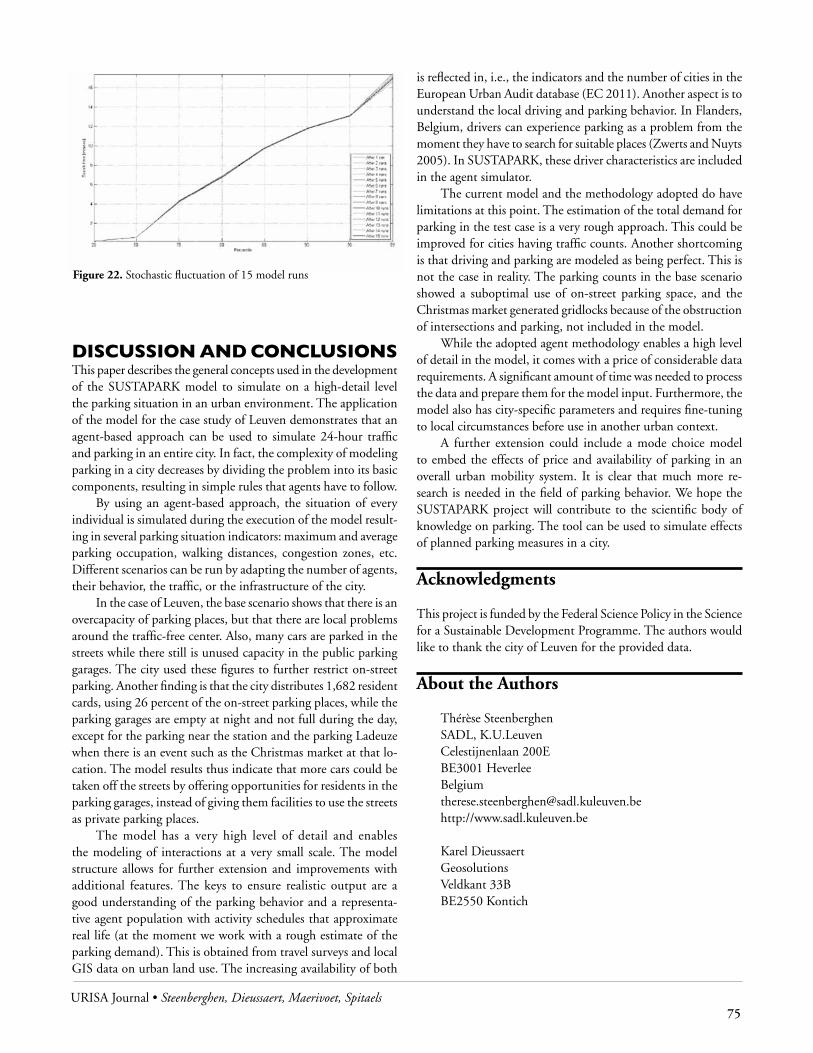
URISA Journal • Steenberghen, Dieussaert, Maerivoet, Spitaels 75
dIScUSSIon And conclUSIonSThis paper describes the general concepts used in the development of the SUSTAPARK model to simulate on a high-detail level the parking situation in an urban environment. The application of the model for the case study of Leuven demonstrates that an agent-based approach can be used to simulate 24-hour traffic and parking in an entire city. In fact, the complexity of modeling parking in a city decreases by dividing the problem into its basic components, resulting in simple rules that agents have to follow.
By using an agent-based approach, the situation of every individual is simulated during the execution of the model result-ing in several parking situation indicators: maximum and average parking occupation, walking distances, congestion zones, etc. Different scenarios can be run by adapting the number of agents, their behavior, the traffic, or the infrastructure of the city.
In the case of Leuven, the base scenario shows that there is an overcapacity of parking places, but that there are local problems around the traffic-free center. Also, many cars are parked in the streets while there still is unused capacity in the public parking garages. The city used these figures to further restrict on-street parking. Another finding is that the city distributes 1,682 resident cards, using 26 percent of the on-street parking places, while the parking garages are empty at night and not full during the day, except for the parking near the station and the parking Ladeuze when there is an event such as the Christmas market at that lo-cation. The model results thus indicate that more cars could be taken off the streets by offering opportunities for residents in the parking garages, instead of giving them facilities to use the streets as private parking places.
The model has a very high level of detail and enables the modeling of interactions at a very small scale. The model structure allows for further extension and improvements with additional features. The keys to ensure realistic output are a good understanding of the parking behavior and a representa-tive agent population with activity schedules that approximate real life (at the moment we work with a rough estimate of the parking demand). This is obtained from travel surveys and local GIS data on urban land use. The increasing availability of both
is reflected in, i.e., the indicators and the number of cities in the European Urban Audit database (EC 2011). Another aspect is to understand the local driving and parking behavior. In Flanders, Belgium, drivers can experience parking as a problem from the moment they have to search for suitable places (Zwerts and Nuyts 2005). In SUSTAPARK, these driver characteristics are included in the agent simulator.
The current model and the methodology adopted do have limitations at this point. The estimation of the total demand for parking in the test case is a very rough approach. This could be improved for cities having traffic counts. Another shortcoming is that driving and parking are modeled as being perfect. This is not the case in reality. The parking counts in the base scenario showed a suboptimal use of on-street parking space, and the Christmas market generated gridlocks because of the obstruction of intersections and parking, not included in the model.
While the adopted agent methodology enables a high level of detail in the model, it comes with a price of considerable data requirements. A significant amount of time was needed to process the data and prepare them for the model input. Furthermore, the model also has city-specific parameters and requires fine-tuning to local circumstances before use in another urban context.
A further extension could include a mode choice model to embed the effects of price and availability of parking in an overall urban mobility system. It is clear that much more re-search is needed in the field of parking behavior. We hope the SUSTAPARK project will contribute to the scientific body of knowledge on parking. The tool can be used to simulate effects of planned parking measures in a city.
Acknowledgments
This project is funded by the Federal Science Policy in the Science for a Sustainable Development Programme. The authors would like to thank the city of Leuven for the provided data.
About the Authors
Thérèse Steenberghen SADL, K.U.LeuvenCelestijnenlaan 200EBE3001 [email protected]://www.sadl.kuleuven.be
Karel DieussaertGeosolutionsVeldkant 33BBE2550 Kontich
Figure 22. Stochastic fluctuation of 15 model runs

76 URISA Journal • Vol. 24, No. 1 • 2012
[email protected]://www.geosolutions.be
Sven MaerivoetTransport & Mobility LeuvenDiestsesteenweg 57BE3010 [email protected]://www.tmleuven.be
Karel Spitaels Transport & Mobility LeuvenDiestsesteenweg 57BE3010 [email protected]://www.tmleuven.be
References
Anderson, S., and A. de Palma. 2007. Parking in the city. Papers in Regional Science 86(4): 621-32.
Arentze, T., and H. Timmermans. 2005. Information gain, nov-elty seeking and travel: A model of dynamic activity-travel behavior under conditions of uncertainty. Transportation Research Part A 39: 125-45.
Axhausen, K. W., and J. W. Polak. 1991. Choice op parking—stated preference approach. Transportation 18(1): 59-81.
Benenson, I. 1998. Multi-agent simulations of residential dynam-ics in the city. Computers, Environment and Urban Systems 22(1): 25-42.
Benenson, I. 1999. Modeling population dynamics in the city: From a regional to a multi-agent approach. Discrete Dynam-ics in Nature and Society 3(2-3): 149-70.
Benenson, I., S. Aronovich, and S. Noam. 2005. Let’s talk objects: Generic methodology for urban high-resolution simulation. Computers, Environment and Urban Systems 29(4): 425-53.
Benenson, I., K. Martens, and S. Birfir. 2008. PARKAGENT: An agent-based model of parking in the city. Computers, Environments and Urban Systems 32: 431-39.
Crooks, A., C. Castle, and M. Batty. 2008. Key challenges in agent-based modeling for geo-spatial simulation. Computers, Environments and Urban Systems 32(6): 417-30.
European Commission. Directorate-General regional policy. The urban audit. Http://www.urbanaudit.org, accessed October 30, 2011.
Hess, S., and J. Polak. 2004. Mixed logit estimation of parking type choice. Presented at the 83rd Annual Meeting of the Transportation Research Board, Washington, DC.
Hess, S., and J. Polak. 2005. Mixed logit estimation of parking type choice. Imperial College. London, working paper.
Laurier, E. 2005. Searching for a parking space. Intellectica 2-3(41-42): 101-16.
Litman, T. 2008. Parking management: Strategies, evaluation and planning. Victoria Transport Policy Institute.
Maerivoet, S., and B. De Moor. 2005. Cellular automata models of road traffic. Physics Reports 419(1): 1-64.
Marsden, G. 2006. The evidence base for parking policies—a re-view. Transport Policy: Special Issue on Parking 13(6): 447-57.
Martens, K., and I. Benenson. 2008. Evaluating urban parking policies with agent-based model of driver parking behavior. Transportation Research Record 2046: 37-44.
Shiftan, Y. 2008. The use of activity-based modeling to analyze the effect of land-use policies on travel behavior. Annals of Regional Science 42(1): 79-97.
Shoup, D. 2006. Cruising for parking. Transport Policy 13: 479-86.
Teknomo, K., and K. Hokao. 1997. Parking behavior in central business district—a case study of Surabaya, Indonesia, Eastern Asia. Society for Transportation Studies Journal 2(2): 551-70.
Thompson, R., and A. Richardson. 1998. A parking search model. Transportation Research A 32(3): 159-70.
Torrens, P. M., and I. Benenson. 2005. Geographic automata systems. International Journal of Geographical Information Science 19(4): 385-412.
Train, K. E. 2003. Discrete choice methods with simulation. Cambridge University Press. Available online at http://elsa.berkeley.edu/books/choice2.html.
Vlaamse Overheid. 2008. Vademecum duurzaam parkeerbeleid, Departement Mobiliteit en Openbare Werken Afdeling Beleid Mobiliteit en Verkeersveiligheid.
Zwerts, E., and E. Nuyts. 2005. Ministerie van de Vlaamse Gemeenschap. Onderzoek verplaatsingsgedrag Vlaanderen; Rapport OVG stadsgewesten, Vlaams-Brabant (2000-2001).

URISA Journal • Zellner, Lyons, Hoch, Weizeorick, Kunda, Milz 77
IntRodUctIonPlanning for complex human-environmental systems requires that decision makers are able to make sense of system complexity. A system is complex when its parts (e.g., residents, developers, farmers, biophysical features) interact selectively with each other through direct actions and through reactive feedbacks, creating dynamic and spatial interdependence (Holland 1995, Miller and Page 2007). Because present interactions change the way in which interactions may occur in the future, uncertainty is inher-ent in complex systems (Axelrod and Cohen 1999). Planning can effectively prepare us to adapt to a range of plausible futures by understanding and building on this complexity, allowing it to inform a community’s intentions about what combination of policy goals to adopt and use. The predominant planning approach to environmental problems involves forming diverse stakeholder committees, focusing on fair representation of dif-ferent viewpoints—a critical aspect of any democratic process. Less attention, however, is placed on understanding the various layers of complexity they face. The first layer is the complexity of the system they are planning for. Individual use of a shared resource interacts with use by others, making it hard to trace causal impacts through the web of interactions, especially when the shared resource also is complex and responds in uncertain ways to human-induced stresses (e.g., groundwater). Cumula-tive effects can appear mysterious. The second layer is the social complexity generated by members’ own diversity of backgrounds, beliefs, interests, perceptions, and data, which informs the way that they interact with each other for collective decision mak-
Modeling, learning, and Planning together:An Application of Participatory Agent-based Modeling to
Environmental Planning
Moira L. Zellner, Leilah B. Lyons, Charles J. Hoch, Jennifer Weizeorick, Carl Kunda, and Daniel C. Milz
Abstract: County and regional government agencies use stakeholder committees to ensure representation of diverse interests when planning, but these representatives often are not trained to understand the complexity inherent to human-environmental issues (e.g., groundwater management). Planning professionals use computer models to simulate the interaction effects of different plan-related policies, but most are “black boxes” to stakeholders, who, therefore, are forced to trust the simulations without understanding human-environmental complexity, reducing the opportunities for effective solution building. Agent-based models can represent decisions and environmental dynamics in a rule-based form that invites nonexpert users’ involvement in both developing the model and meaningfully interpreting its outputs. We conducted a series of collaborative and developmental agent-based modeling meetings with stakeholders and planners in a rapidly suburbanizing area facing groundwater shortages. Stakeholders learned how to use the models, understand the relationships among the components, interpret the outputs based on these relationships, and suggested modifications with new insights. The enhanced understanding of complex interactions reduced early commitments to policy solutions as stakeholders jointly explored the range of possible outcomes. These results show that agent-based modeling holds promise for use in collaborative planning exercises.
ing. Self-interest and partial understanding of the system they are planning for often leads stakeholders to focus exclusively on individual impacts, exaggerating their salience, and overlooking critical interactions. Policy makers may focus prevention or miti-gation efforts on a single type of user or use (e.g., farmers) that does not remedy systemic depletion pressure from other sources (e.g., residential subdivision growth).
Anticipating these difficulties, stakeholders may use a variety of visualization tools to estimate and display potential future ef-fects of different plans. Popular and easy-to-use tools often mislead stakeholders when applied to complex problems. Less familiar and more demanding simulation tools may better estimate future in-teraction effects of different plan-related policies and expectations, but they require hiring expert modelers to collect high-quality data to inform the models, build the models, conduct the simulations, and interpret their results. Outside expertise relies on stakeholders’ trust, but because stakeholders do not understand the simulation of future effects in their own terms, their confidence flows from professional reputation, not understanding. Off-loading plan simulation onto outside experts does not allow for stakeholder examination of policy goals and alternative plans in light of their implications for the future.
Planning theorists and analysts have made the case for col-laborative plan making when confronting complex problems, the argument being that collaboratives can better learn to conceive, assess, and choose among options for the future (Innes and Booher 2010). Most studies focus on the design of plan-making institu-tions and stakeholder involvement to reconcile the complexity
78 URISA Journal • Vol. 24, No. 1 • 2012
of social and political goals (Innes et al. 2007, Susskind and Cruickshank 1987). Others study the methods and tools used to improve the quality of collaboration (Forester 1999, 2010). In this article, we add to this area of inquiry by studying how agent-based modeling can contribute as a participatory model-ing tool for collaborative planning, examining how it affects the learning processes underpinning the ability to explore complex environmental problems.
Participatory Modeling and Collaborative Planning Participatory model building involves not only expert modelers but also stakeholders and public officials in conceptualizing and building models, interpreting their results, and using them to sup-port decision making. When used as a support for collaborative planning, participatory modeling has the theoretical advantages of cultivating a shared understanding and better framing of complex problems and informing problem-solving judgments, by inviting participants to explore potential outcomes and learn how the assumptions and beliefs built into the model result in the simu-lated outcomes. This collective modeling improves the chances that the plans proposed will be supported and implemented, as diverse voices are heard and beliefs are adjusted to a common understanding of the shared vulnerability to the deterioration of common environmental resources (Tidwell and van den Brink 2008, Zellner 2008). While valuable in theory, in practice, model literacy and use typically remains the domain of the expert mod-elers who regularly use computer simulations in their work to better understand the systemic processes and trade-offs involved in human-natural systems. In their zeal to create “accurate” rep-resentations of complex human-environmental change, experts tend to generate tools that only they can use. These tools are not designed for use by professional planners and civic stakeholders. Modeling experts typically present their simulations to planning committees late in the planning process to show the impacts of competing, already-developed scenarios, but the audience rarely grasps how they were generated, constituting “black boxes” that are not open to public scrutiny (Zellner 2008). Some of the obstacles to regularly and fruitfully using models for collabora-tive resource management and environmental planning include: • The requirement of extensive professional training to
conceptualize, build, and use models (Joerin and Nembrini 2005, McIntosh et al. 2007, Tidwell and van den Brink 2008);
• The difficulty to adapt models to specific contexts and to generalize across contexts because of the expensive expertise and data required (Joerin and Nembrini 2005, Borowski and Hare 2007, Tidwell and van den Brink 2008, van Herzele and van Woerkun 2008);
• Computer applications that are unfriendly to nonexpert modelers, preventing the involvement of stakeholders and managers in model construction and interpretation (Borowski and Hare 2007, McIntosh et al. 2007, Zellner 2008);
• The tension between inherent limitations of models as exploratory tools and the requirement of accurate predictions imposed by political processes (Joerin and Nembrini 2005, Borowski and Hare 2007, Zellner 2008); and
• The power imbalances that allow special-interest groups to exert too much influence on the process, while underrepresented groups remain marginal (Tidwell and van den Brink 2008).
As a consequence of these barriers, modeling efforts often fail to lead to the learning necessary for changes in policy and behavior to occur because citizens find it difficult to interact with the model and interpret its outputs (Zellner 2008). Moreover, the outcomes predicted by “black box” simulation tools are strongly questioned by participants because the assumptions and interactions within the simulation are not revealed, especially when the results do not match the participants’ beliefs and values (Dasgupta et al. 2010). As a result, participants rarely incorporate their own values and specialized knowledge into the spatial and dynamic models, or derive useful insights from the simulations to inform discussions that advance policy changes in the direction of socioecological improvement. Such collaborative processes eventually may lead to consensus but not necessarily to a better understanding of how the problem being addressed is complex and to policy that adapts policy goals to this new understanding, i.e., to learning. Helping stakeholders learn about complex environmental prob-lems requires new skills and tools to support reasoning about complexity. Such reasoning ability would enable stakeholders to more readily recognize different forms of knowledge, scales, and interactions represented in their collective endeavor, and to expand their understanding of the problem from a propositional view of how individual pairs of variables interact to a view that acknowledges the networked structure of influences on variables of interest. Stakeholders thus would be better equipped to ex-amine the relative influence of different variables both in terms of effect and relative manipulability, allowing communities to avoid making planning decisions that might seem to lead to so-cioecological improvement but to comparatively little net effect. The ability to reason about complexity would lead, therefore, to the cocreation of both knowledge and beliefs about appropriate steps toward resource sustainability, beyond the conditions for effective participation that are typically the focus of planning literature (Steyaert et al. 2007, Zellner 2008).
Our motivation is to find ways to enhance collaborative environmental planning processes with the use of modeling tools that can support learning about the complexity of the socioeco-logical system and thus promote innovation of policy. We use a different kind of approach, which follows from an epistemology that privileges creative exploration over establishing proof. Rather than using models to accurately predict future impacts of deci-sions, we use models as prosthetic thinking devices to support the rapid creation and exploration of scenarios that can lay bare previously hidden interaction effects. Prediction works well for linear systems, where models can be used to perform calculations

URISA Journal • Zellner, Lyons, Hoch, Weizeorick, Kunda, Milz 79
to estimate a future state of the system, and where the only limita-tion is data accuracy and availability. With complexity, attempting such projections is a futile effort. Even with accurate data readily available, the interdependence of system parts greatly reduces our ability to predict future states, as a variety of plausible futures may emerge from identical processes. In this case, exploring the range of possibilities and how they can emerge from underlying processes is more supportive of planning for complexity and un-certainty than trying to match history and projecting it into the future in a linear manner (Brown et al. 2005). This exploration ap-proach also aligns well with the inquiry-driven learning processes that often are at play in nonclassroom learning settings (Bell et al. 2009). With an exploratory approach, disparate stakeholders may learn how reliance on a shared aquifer, for example, makes each vulnerable to the level and location of water use by others and how these interactions vary depending on environmental conditions and water-use rules and behavior. Their assumptions and beliefs thus are tested as they explore the interconnections among water users with the natural resource illustrated by the model. With this understanding, they may use the model to inform decisions about water-management strategies and programs, and to brainstorm innovative strategies not previously conceived. With interactive, software-based models, it becomes harder to ignore the fact that models are a part of the planning-activity system, playing a role in mediating the communication of knowledge between partici-pants and in shaping the unfurling of the collaborative process (Kaptelinin 1996).
Designing a Participatory Modeling and Learning Process for Environmental PlanningOur aim was to produce a collaborative planning experience that would (1) help nonexperts better understand complex human-natural interactions and to use that knowledge to (2) engage in more truly collaborative and creative planning activi-ties. Our methodology is informed by Design-Based Research (DBR) (Cobb et al. 2003), which is especially useful when at-tempting to create new educational interventions for real-world settings. Following are some of the design guidelines, drawing from recommendations in the literature on learning sciences, social learning and collaborative planning, complex systems, and decision-support systems:(1) Design guidelines for how to aid nonexperts understand
complex human-natural systems: • Preserve a systems outlook throughout: Nonexpert
understanding of complexity tends to focus on visible structures and assumptions of central control and single causality, rather than on an in-depth awareness of how system components interact at different temporal or spatial scales to give rise to the system’s functions. Consequently, novices’ common sense is overly simplistic and does not apply well to natural systems where time lags and invisible feedback generates counterintuitive effects (Hmelo et al. 2000, Hmelo-
Silver et al. 2007a). Research shows that introduction to even highly simplified systemic models sensitizes one to possible sources of complexity and allows one to perceive those sources even in new problem domains (Goldstone and Sakamoto 2003). Understanding complexity allows participants to reuse that knowledge and transfer it to other situations (Hmelo et al. 2000, Hmelo-Silver et al., 2007a). Therefore, our goal here is not to help stakeholders memorize the structure of one particular web of influences, but to sensitize them so that when they face a planning problem they resist causal reductionism and are likely to adopt a perspective that acknowledges that there is likely to be a web of influences that needs to be considered.
• Make invisible interaction effects visible: To facilitate understanding of behavior and function in a complex system (see previous point), learning activities need to provide participants with opportunities to experience these systems through the use of computational tools and simulations that highlight the relevant interactions (Hmelo et al. 2000, Jacobson and Wilensky 2006, Hmelo-Silver et al. 2007a). Additionally, different perspectives, beliefs, and assumptions need to be made explicit among stakeholders, for which the computational tools need to cross boundaries between communities of knowledge and practice to represent them in explicit form (Maurel et al. 2007). Tools can greatly shape how people reason about problems (Papert 1980) and can change how people reason about complex systems (Wilensky and Resnick 1999) in part by making previously unconsidered elements accessible.
• Enable hands-on model building and exploration: Research shows that hands-on interaction, scaffolding, and iteration that allows for alternating analysis and model building with reflection and constructive discussion builds both the cognitive and the social skills of a group (Hmelo et al. 2000, Jacobson and Wilensky 2006, Hmelo-Silver et al. 2007b, Maurel et al. 2007, van Herzele and van Woerkun 2008). Learners need to be actively engaged in design and modeling activities to learn to reason about complex systems, and in exploration and critique of successive model versions to move from appearance-based to functional models (Wilensky and Resnick 1999, Hmelo et al. 2000, Klopfer et al. 2005, Hmelo-Silver and Barrows 2006, Papaevripidou et al. 2007). It takes time for these skills to develop and be incorporated into the practical aspects of decision making for a specific place (Hmelo et al. 2000, Jacobson and Wilensky 2006).
(2) Design guidelines for how to engage groups in more truly collaborative and creative planning activities:• Include diverse participants: Diversity of viewpoints
and experiences improves the scope and range of ideas for understanding and solving complex environmental

80 URISA Journal • Vol. 24, No. 1 • 2012
problems (Maurel et al. 2007, Page 2007), an ideal of most collaborative planning activities.
• Coconstruct a model to follow the group’s line of inquiry: The elements stakeholders may want to include in a model, and the kinds of questions they will wish to investigate using the model, depends significantly on the idiosyncrasies of the diverse group of participants. To maintain motivation when engaged in inquiry learning, learners must be allowed to pursue problems of interest to them (Blumenfeld et al. 2006). For this reason, it is important to allow the group’s interests to direct which elements to add and which outcomes of interest to attend to.
• Foster small group collaboration: Learning to collaborate is fundamental for complex problem solving, as an individual skill to become informed citizens, and as a collective form of computation (Barron 2000, 2003; Hmelo-Silver et al. 2007b, p. 2007), and to foster a sense of responsibility for both individual and group work outcomes (Johnson and Johnson 1989). Small group size is important for effective dialogue (Borowski and Hare 2007), as is alternating individual and group work to allow for both individual and collective viewpoints to be developed (Hertz-Lazarowitz 1992).
• Alternating between abstract and detailed models: The use of detailed geographic information is perceived as more realistic and accurate. Such detail may overwhelm novices especially if they are not strong learners and put them at risk of misinterpreting simulations, preventing effective exploration and understanding of the behavior and function of a system (Hmelo et al. 2000, Goldstone and Sakamoto 2003). Alternating between stylized, abstract models and detailed representations may allow a better transfer of knowledge about basic principles of complex systems to other realms (Goldstone and Sakamoto 2003). Given that collaborative processes may engage different types of learners, it therefore becomes important to provide a suite of modeling tools that alternates between abstract and detailed representations.
Based on these recommendations, we designed a four-session developmental and participatory modeling approach with a group of diverse planning stakeholders who had helped develop a water-resource management plan for a suburban county near Chicago, Illinois. The goal of the activity was to give the stakeholders the opportunity to recognize and assess the impacts associated with the implementation of the elements of their proposed plan. The goal of our activity design was to enhance stakeholder delib-erations and collective planning judgments by promoting joint learning of the complexity of their water problem through the use of a series of computational models that integrated land-use and water-use decisions with aquifer dynamics. We chose agent-based modeling (ABM) to represent the complex socioecological system because their rule-based structure and explicit representation of
interactions among relevant actors and environmental processes may improve novice understanding of how complex systems work, and thus facilitate involvement in setting values and modifying rules, inspiring trust in the modeling process (Hmelo-Silver et al. 2007, Zellner 2008).
Assessing Learning in PlanningThe effectiveness of collaborative planning processes to promote learning and better policy—with or without modeling—are rarely assessed (Joerin and Nembrini 2005, Deyle and Schively Slotterback 2009, Laurian and Shaw 2009), in great part because the field of planning has not developed effective measures of learning (Deyle and Schively Slotterback 2009). Some studies have used the standard deviation of opinion (Schively 2007) or an adjustment of expectations (Deyle and Schively Slotterback 2009) to trace convergence, apparently adopting a sociocultural perspective on learning (Greeno et al. 1996) similar to the theory of learning known as “convergent conceptual change” (Roschelle 1992). However, convergence is not always equivalent to learn-ing, only to consensus or persuasion. The participatory modeling literature provides assessment frameworks that are more in line with critical examination of beliefs and the integration of diverse forms of knowledge (e.g., Jones et al. 2009, Smajgl 2010), which places a higher premium on framing learning as a more cogni-tive process of changing internal mental models (Johnson-Laird 1983). We acknowledge the value of framing learning from both sociocultural and cognitive theoretical perspectives, as each highlights different aspects of the processes at play. We focus the assessment on how stakeholders individually and jointly learn to reason about the complexity of environmental problems and how they apply that reasoning to collectively formulate plans and policies for socioecological improvement. We collected data that would speak to each of these areas.
In many respects, the activities that take place within col-laborative planning meetings strongly resemble what is known in the educational world as Problem-Based Learning (PBL), where groups of learners are given a real-world problem to solve and go through an iterative series of facilitator-guided problem-solving steps (e.g., problem definition, hypotheses generation, data collection and analysis, reflection and discussion on potential solutions) (Evensen and Hmelo 2000). We adapted some of the methods used to track learning in such contexts (e.g., pretest and post-test surveys, analysis of videorecordings, and observations of meetings) to assess how our participatory ABM intervention affected the cognitive grasp of complex environmental problems, the resulting planning judgments, and the joint collaboration around the implementation of the plans. We draw from learn-ing sciences and resource management literature to assess various dimensions of learning about complex systems (Wilensky and Resnick 1999, Hmelo et al. 2000, Jacobson 2001, Jacobson and Wilensky 2006, Hmelo-Silver et al. 2007), and the effectiveness of collaborative approaches in changing stakeholder individual beliefs and preferences toward collective goals of sustainability (Roschelle 1992, Siebenhüner 2005, Blackmore 2007, Deyle and

URISA Journal • Zellner, Lyons, Hoch, Weizeorick, Kunda, Milz 81
Schively Slotterback 2009, Jones et al. 2009, Smajgl 2010), and policy innovation and support (Borowski and Hare 2007, Tidwell and van den Brink 2008). We evaluated changes in participants’ tendency and ability to do the following:• Reason about complexity to inform planning decisions, as they
try to explain the causes of the impacts they observe in the simulations across temporal and spatial scales, shift from a structural to a functional perspective of the problem, acknowledge the potential of planning outcomes to be affected by multiple factors, and generate potential solutions for socioecological improvement that are sensitive to the webs of influence in the system;
• Engage in collaborative deliberation, where adversarial emphasis is replaced by common conception of the problem and collective goal achievement as a result of understanding interdependences in the webs of influence in the system;
• Generate creative and viable implementation plans for socioecological improvement, as stakeholders trust the validity of the lessons learned about the complexity of the problem through modeling and translate these lessons into plan development, adoption, and implementation; and
• Use modeling to explore the planning problem and its possible solutions, as they make judgments about inputs to learn how they shape outcomes, interpret outputs, communicate effectively about phenomena revealed by modeling and discuss their implications for planning.
The remainder of this paper presents the case study in which this approach was applied, the details of our intervention, and the findings around the four dimensions mentioned previously. Within each dimension, we describe what we learned and how we learned it, and the implications for participatory modeling in planning contexts. We conclude with future directions for research and for practice using these tools.
thE contExt: GRoUndwAtER dEPlEtIon In noRthEASt IllInoISGroundwater is an open-access resource, meaning that users cannot be excluded from tapping into it without incurring very high costs, and each unit consumed by a user cannot be used by any other user. As withdrawals cause cones of depression around wells, the groundwater decline affects neighboring areas, thus making it more costly for others to extract water from the aqui-fer. Because it is so costly to exclude others from accessing the resource, the incentives are there to deplete it in a literal race to the bottom. Physical and socioeconomic factors contribute to the complexity of groundwater resources. On one hand, groundwater is connected to surface water systems and their replenishment and discharge rates are influenced by biophysical conditions that vary over space and time (e.g., hydraulic conductivity, aquifer depth, aquifer confinement, water levels, soil conditions, vegetation, pre-cipitation). This dynamic interaction makes it hard to anticipate
how the resource will respond to either physical changes or human use, or determine how much water is available for a variety of uses. Hydrological studies heavily rely on data collection on various points of an aquifer, but connecting the data over time and space into a dynamic understanding is not straightforward. Land-use decisions also are intimately linked to the spatial and temporal patterns of groundwater levels. When multiple users depend on the resource, differing beliefs of management costs and benefits make it hard to identify the causes of decline and define the re-sponsibility for action. Further complicating the implementation of appropriate measures is the intervention of legal processes where decisions are made based on precedent and resources for litigation, rather than on an understanding of resource dynamics. Therefore, planners and stakeholders need to consider land-use patterns and the factors driving them, how water-use patterns emerge from the spatial distribution of economic activity, and how groundwater responds to these stresses, to ultimately understand groundwater depletion and coordinate action to reverse it (Tidwell and van den Brink 2008, Zellner 2008).
The prospect of groundwater shortages is very present in the suburban areas of Chicago, even when the region has abundant water resources. Lake Michigan diversions are infeasible eco-nomically, logistically and legally because of the Great Lakes–St. Lawrence River Water Resources Compact (McHenry County 2009, Council of Great Lakes Governors 2011). Consequently, many communities that are not currently connected to this surface water source are left to rely only on their aquifers for water supply. McHenry County is a rapidly urbanizing area in northeast Illinois facing this challenge (see Figure 1). Groundwater concerns in the county include increased groundwater pumping, which results in declining levels for consumption and for recharge of surface water bodies, and potential for groundwater contamination from chang-es in land use and contaminated materials spilled on the surface. Responding to this challenge, the county government convened a Groundwater Task Force in 2008 to prepare a series of recom-mendations for groundwater protection. The group included representatives from local units of government, planners, members of councils of governments, county officials, real estate profes-sionals, contractors, and environmental nonprofits. The resulting Water Resources Action Plan (WRAP) offers general guidelines for future development assumed to benefit the natural environment, but does not specify implementation of these recommendations or examine how they would work when translated into practice. Despite these planning efforts, conflicts persist around defining implementation strategies because of inadequate knowledge of the interaction effects in complex resource use. So, for example, while the plan encourages conservation development to enhance recharge, it does not give any indication of how the scale of such development might indeed negatively affect recharge, or how it compares to drawdown rates generated by this and other types of development. Stakeholders who shared broad sustainability goals continued to describe divergent narrowly focused solutions that did not recognize or respond to the complex interaction among current and future users with the shared resource. These were

82 URISA Journal • Vol. 24, No. 1 • 2012
the stakeholders we hoped might use ABM to improve plans to coordinate future water use in McHenry County.
MEthodIn line with the design recommendations we distilled for encour-aging novices to learn about complex systems through participa-tory modeling and for supporting collaborative planning (see “Designing a Participatory Modeling and Learning Process for Environmental Planning”), we sought to work with a diverse group of 16 stakeholders in a series of meetings that alternated between model building and discussion, exposing participants to a progression of models with different degrees of detail about the interaction between land-use decisions, water use, and ground-water levels. With the models, stakeholders explored policy and behavioral scenarios, discussed implications for planning and policy, and gave feedback on future model versions. To facilitate complex systems learning, stakeholders were asked to work in small groups of two or three people per computer, so that they would engage more directly with model exploration, and then reconvene to discuss the findings and planning implications in the larger group. We assessed how stakeholders learned to reason about the complexity of their environmental problem by engaging in participatory ABM, how they derived insights from this experience, and how these insights affected their positions about the problem and potential solutions and their planning and policy discussions.
ParticipantsWe approached members of the Task Force who had played a role in developing the WRAP for McHenry County (see “The Context”). The stakeholders now faced the challenge of imple-menting a combination of policies and programs. We offered to assist them in learning how to use ABM to translate the WRAP into implementation. Sixteen members of the Task Force agreed to participate in our study. Many of them were homeowners in McHenry County, and they represented public officials, envi-ronmental advocacy organizations, and resource management professionals. The group did not contain any representatives of real estate, business, or private water operator interests.
Participatory Modeling ProcessWe conducted a series of four collaborative planning meetings over a three-month period with our participants. Prior to the first meeting, the viewpoints of the group generally were favor-able toward the recommendations included in the WRAP. The meetings were structured around a scaffolded learning process that allowed the participants to become familiarized with the use of ABM and how it can be used to understand the complexity of land-use and groundwater interactions (see Table 1). Stakeholders worked individually and in small groups around a progression of models—from highly abstracted models of traffic, of land-use change and of land-use and groundwater interactions, to geo-graphically detailed integrated land-use and groundwater models of McHenry County—to recognize and assess the interactive im-pacts of different implementation strategies. Stakeholders learned how to use the models, understand the relationships among the
Figure 1. McHenry County, Illinois

URISA Journal • Zellner, Lyons, Hoch, Weizeorick, Kunda, Milz 83
Table 1. Structure, timing, and activities of the four participatory modeling meetings
Meeting 1 (November 18, 2010): Meeting 2 (December 2, 2010):• Structured brainstorming activity
• Stakeholders in small groups define and link problem causes and solutions
• Researchers help combine group brainstorms to uncover complexity and conflicts
• Researchers introduce stakeholders to ABM (Traffic Basic Model)• Interface overview (sliders, graphs, displays)• Concepts of complexity (emergence)• Rudimentary programming, changing rules, and observing
outcomes
• Researchers guide stakeholders’ “play” with ABM (SOME, then SOME-GW)• Interface overview (new components)• Discussion and exploration of assumptions, rules, and inter-
action effects• Stakeholder explanation of observed effects
• Researchers elicit stakeholder feedback for further model de-velopment
• Administered homework for individual work (SOME-GW)
Meeting 3 (January 12, 2011): Meeting 4 (January 26, 2011):• Researcher facilitates discussion on individual homework• Researcher demonstrates application of ABM to same prob-
lem in a different geography, how to use data to inform and adapt models
• Stakeholders use worksheets to provide feedback on agents, rules, and parameters to help codefine the detailed model simulations
• Researcher presents summary of collectively determined changes made to geographically based model and simulation results for WRAP scenarios
• Group discussion on implications for WRAP implementation and policy innovation• What worked and what didn’t? Why?• Alternative policy scenarios
• Researchers guide stakeholders “play” with ABM (stylized ver-sion of SOME-GW for McHenry County) to confirm results and explore new policies
• Group discussion on WRAP implementation and future di-rections
Figure 2. Interface of Netlogo Traffic Basic model (Wilensky 1997)

84 URISA Journal • Vol. 24, No. 1 • 2012
components, interpret the meaning of the outputs based on these relationships, and modify the models with new insights from the discussions (Table 1). For some of the activities, stakeholders were given worksheets and cards to take notes and aid in reflection and discussion in the larger group.
Meeting 1 The purpose of the first meeting was to make the problem defini-tion and its complexity explicit and expose the stakeholders to tools that support the exploration of complexity and how they can be used to derive insights for behavioral and policy changes. In this meeting, participants worked in small groups to define the causes for the groundwater problems in the county, outline possible solutions, and identify relevant interactions that might either exacerbate the problem or introduce barriers for the effec-tive implementation of solutions to the problem, using note cards to organize the discussion. As the complexity of implementation became apparent, it provided the basis for introducing ABM as a way to explore the implications of such complexity. The first agent-based model that stakeholders were presented with is the Traffic Basic model (Wilensky 1997), included in the library of the Netlogo ABM platform (Wilensky 1999) (see Figure 2). We selected this model as a relatively simple way to introduce participants to the Netlogo interface (visual display, plots, slid-ers, buttons, monitors), identify agents (cars), and examine how local interactions (through acceleration and deceleration as they encounter cars ahead of them) may give rise to systemwide effects (traffic jams). The researchers facilitated stakeholders’ explora-tion and modification of small sections of the code to show how interaction rules can be represented and changed in these models. This activity was followed by a mediated group reflection on how individual driving behavior could lead to the formation of traf-fic jams and discussion on implications for behavioral changes and driving education, thus illustrating for the stakeholders how ABMs may be used as springboards for generating policy ideas.
Meeting 2 In this meeting, the intent was for stakeholders to become ac-quainted with the complexity of land-use change and, ultimately, how patterns of urbanization are tied to water consumption and consequently to aquifer conditions. Exploring these interconnec-tions with the model would enable them to derive insights about the relative effectiveness of different planning measures for the protection of water resources. Stakeholders were first exposed to a simple land-use model based on the SOME model (Rand et al. 2002, Brown and Robinson 2006) and some aspects of the WU-LUM model (Zellner 2007). It includes resident and service center agents that make location decisions based on their preferences for such things as urban and natural amenities. The residential agents (represented by yellow houses in Figure 3 (a)) are created at each time step and make location decisions based on the location of service centers (represented as red squares in Figure 3 (a)), the natural beauty of the landscape (represented by varying colors of green cells), and zoning restrictions that limit the number of
residential agents that can locate in each cell. Service centers are created as residential population grows, based on the location of the newest residents. Depending on the model settings, develop-ment may deteriorate the natural beauty of its surroundings. The feedback between residential development, commercial develop-ment, and natural beauty thus affects subsequent directions of development. Stakeholders were guided in their exploration with this model to understand the effects of the various parameters in the model (e.g., growth rate, amount of information about potential location sites, preference for proximity to service centers versus natural beauty, the feedback of environmental degradation, density restrictions). They investigated these effects by using the visual display (Figure 3(a)) and plots of simple metrics of urban expansion, average happiness of the residents, and regional eco-logical quality. The researchers facilitated the group’s discussion and formulation of explanations for how localized interactions among residents, service centers, and natural beauty could lead to different land-use and environmental patterns.
Facilitators then showed the stakeholders how to use the SOME-GW model (Zellner 2011) to explore how land-use pat-terns might affect groundwater levels. The SOME-GW model couples groundwater dynamics with the land-use component of SOME. The groundwater component is represented through diffusion rules between a patch and its immediate neighbors, based on Darcy’s law of flow and taken from the WULUM and WULUMOD models (Zellner 2007, Zellner and Reeves 2010). The emerging rate of flow and groundwater gradient (represented by varying colors of blue cells in Figure 3 (b) vary with aquifer characteristics such as boundary conditions and hydraulic con-ductivity, which are parameters of the model. Residential agents now are able to pump water from the groundwater system at a consumption rate specified by the user, creating cones of depres-sion that affect the availability of water for themselves and for neighboring agents. The model illustrates which residents are in deficit (shown in brown in Figure 3 (b) when water levels drop beyond a threshold. Additionally, groundwater levels may affect the location of new residents through the agent’s sensitivity to groundwater decline. Following a preliminary introduction to the SOME-GW model, the researchers elicited initial feedback on how the model interface could be made more meaningful for the purposes of plan implementation for groundwater protec-tion, by adding or modifying inputs (e.g., sliders) and outputs (e.g., plots). Requests for input user interface features were, in effect, endorsements of the variables stakeholders most desired to manipulate, and requests for output user interface features indicated the outcomes of most interest to the stakeholders. The stakeholders were given specific instructions for guided explora-tion on their own, to make sense of the mechanisms in the model and the effects of the various model parameters on output patterns of groundwater levels and deficit.
Meeting 3 The purpose of the third meeting was to illustrate how models such as SOME-GW can be adapted to a specific geographic

URISA Journal • Zellner, Lyons, Hoch, Weizeorick, Kunda, Milz 85
context, to help stakeholders provide detailed feedback and in-dicate sources of data to make the model relevant to the issues in McHenry County. The researchers first facilitated a discussion in which participants could discuss their experiences using the first version of SOME-GW provided in Meeting 2 and attempted to explain the resulting patterns through the mechanisms and pa-rameters of the model. Following this discussion, the lead author presented a summary of the application of similar models in a different geographic context—Monroe County, Michigan—ex-plaining how sociodemographic and hydrological data can be used to adapt a stylized version of the model they had explored into a model that is more relevant to their planning efforts. We provided participants with a worksheet listing potential agents, rules, and parameters (many informed by the feedback obtained from the stakeholders in prior meetings) that could be included in a more detailed version of SOME-GW. Participants elaborated from this list, based on their experiences with the preliminary ver-sions of the modeling tools and on their knowledge of the region. We intentionally delayed the elicitation of the desired “interior parts” (agents, rules, and parameters) of the model until after the participants had had enough modeling experience that they would have a conceptual framework to help them organize the relevant information into a model-ready form, with a preliminary understanding of what local interactions were likely to affect the resulting groundwater depletion patterns.
Meeting 4 In the final meeting, participants were presented with simula-tions produced by a revised version of SOME-GW, informed by their feedback and the data suggested in Meeting 3, which were used to test the effects of the policy scenarios inspired by the WRAP that the stakeholders selected as being the most worthy of exploration (see Table 2). The purpose of this meeting was
to allow stakeholders to examine and derive insights from the results of a highly concrete and detailed simulation, and to give stakeholders an opportunity to conduct their own explorations with a simplified, more abstract version of the model (to reduce the distraction of extraneous details and to speed up simulations), and to further discuss planning and policy implications for the county. The SOME-GW had been modified in between Meetings 2 and 4 to include the additions requested by the stakeholders: new actors reflecting the variety of water users in the county, rules for location and assignment of both private and public wells, policy settings specific to the WRAP, and new outputs for water consumption and drawdown. In addition to the visual display (Figure 3 (c)), the model interface included additional graphs of the effects of groundwater drawdown (e.g., average, minimum, and maximum drawdown; area and households in deficit). The simulation results with the detailed model showed that the WRAP scenarios had virtually no impact in preventing widespread groundwater depletion and deficit. The only behavior that made a more substantial difference was reducing the consumption of water per household, which both delayed the onset of the general-ized deficit and reduced the area and level of drawdown. These results were surprising to the stakeholders, who were hoping that the WRAP would have a greater beneficial effect. The research-ers facilitated a discussion in which stakeholders were asked to explain these results, based on the mechanisms and the data in the model. They identified continued growth as being the cause of the problem, but were reluctant to modify this development goal for the county (see more details in the “Findings” section). They then used the simplified model to confirm or question the results obtained with the detailed model. In response to these explorations, a stakeholder proposed a new rule involving the introduction of a policy allowing injection into the aquifer. With the group’s agreement that this was worthy of experimentation,
Figure 3. Visual display of (a) SOME model, (b) SOME-GW model, and (c) SOME-GW with McHenry County data. (Note: brighter shades of green = higher natural beauty, darker shades of blue = higher groundwater levels, red squares = service centers, yellow houses = resident agents, brown houses = residents in water deficit)

86 URISA Journal • Vol. 24, No. 1 • 2012
they then were assisted through an exercise of adding this rule in the model. The stakeholders modified the code and then ran simulations with the new rule to examine its effect. This exercise generated more discussion about planning implications for the county and suggestions for further modeling efforts.
Data Collection and AssessmentWe conducted a pretreatment and post-treatment survey in which participants were asked about their interest in groundwater is-sues, their general knowledge about groundwater systems, and their beliefs about the contributors and solutions to groundwater depletion. We examined the differences in responses between the pretest and post-test surveys to estimate changes in stakeholder understanding of the complexity of the problem of groundwater depletion in their region, their willingness to sacrifice personal gains for collective goals, their commitment to specific solutions, and their understanding of modeling and its application to plan-ning. We also observed interactions and discussions during the meetings and videotaped each meeting and coded the dialogue based on the four learning process and outcome dimensions outlined in the introduction. We used this data to examine how stakeholders learned about complexity by modifying and explor-ing with the models, their level of trust in the tools, and how they used them to create a shared understanding of the problem and of the effectiveness of solutions and to propose new alternatives. We also used the videotapes to identify where major obstacles exist to stakeholder appropriation and meaningful use of these tools in their planning process.
Meeting attendance was uneven. A total of 15 participants agreed to participate, but attendance was sporadic: 13 participants
attended the first meeting, 12 attended the second, eight partici-pants were present for the third, and there were five participants at the final meeting. Only three participants attended all four sessions. The absence of most of the group at the final meeting made beginning-to-end comparisons difficult. Additionally, not all participants took the survey and only four of them completed both the pretest and post-test surveys. The findings we report thus rely mainly on our observation of changes within a single meeting or across two meetings for clusters of participants or occasionally an individual, with some support of survey responses and video-tapes to validate inferences about learning about complexity with ABM and the transfer of this learning to planning judgments.
fIndInGSWe set out to study how stakeholder engagement with ABM in a collaborative setting contributed to the four learning process and outcome dimensions that are relevant to planning for complex environmental problems. We report our findings in relation to each dimension and then offer a brief conclusion describing future research directions.
Reasoning about Complexity to Inform PlanningIn the first meeting, stakeholders learned how agent-based models represent interactions and how these interactions can lead to sys-temwide changes. Active learning ensued in the second meeting as stakeholders found out how adjusting individual preferences for location could yield different land-use patterns and, in turn, affect social utility and natural beauty. Most stakeholders figured out that there was a connection between these scales, but many did not grasp how this was accomplished. When using the styl-ized land-use and groundwater model in Meeting 2, stakeholders
Table 2. Simulation scenarios based on recommendations from the Water Resources Action Plan (WRAP)
Parameters Scenarios
Baseline Urban Growth Boundary
Preserving SARAs (Sensitive Aquifer Recharge Areas)
Preserving SARAs + Conservation Development
Preserving SARAs + Conservation Development + Conservation
WaterPreference for proximity to services over proximity to natural beauty
0.5 0.5 0.5 0 0
Impact of development on natural beauty
0.5 0.5 0.5 0 0
Development boundaries None Municipalities Preserving SARAs Preserving SARAs Preserving SARAs
Water consumption rate (m3/household/year)
361 361 361 361 200
Development impacts re-charge
1 1 1 0 0
URISA Journal • Zellner, Lyons, Hoch, Weizeorick, Kunda, Milz 87
balked as they realized that none of the proposed conservation solutions prevented groundwater depletion. Explorations in the fourth meeting with more detailed models for McHenry County (with new rules and geographic and hydrological data) enhanced the validity of the exercise but did not alter the trial results stake-holders had discovered. By making decision rules and interactions explicit, the models helped stakeholders understand counterin-tuitive systemwide effects that may arise from the interaction of localized decisions and explain the disappointing results:
“ . . . and then there’s the idea that we’re gonna do this and it’s gonna have such a big impact, and it really doesn’t.”
“ . . . this all makes sense actually. What you’re finding makes perfect sense because even if you protect [the sensitive aquifer recharge areas] and do conservation design and do water con-servation you’re still adding residents.”
These quotes illustrate a significant break from the common conception in these areas that residential and commercial growth should be pursued as the main engine of economic development, and that conservation development will make growth sustainable. Acknowledging the lack of viability of the WRAP is necessary (although as we will show, not sufficient) to encourage creative planning.
Ironically, although stakeholders showed possessing a better grasp of the problem, they had difficulty articulating the underly-ing idea of complexity that the models exposed, mostly because of their discomfort with computer modeling. One stakeholder admitted:
“If I had to sit here and explain it, I would have a hard time ex-plaining the background knowledge, this is how we developed it.”
At the last meeting, after identifying the negative effects of growth and considering the possibility of injection as an alterna-tive solution, stakeholders did not see how they could further use modeling to continue illuminating their discussions on planning and implementation for groundwater protection. Moreover, the post-test survey did not show a clear effect on ways of thinking about the problem or its solutions, beyond a tenuous shift toward favoring behavioral changes over regulatory approaches. Although stakeholders expressed satisfaction with using a progression of abstract to detailed models to learn about ABM and its application to planning for water protection, the complexity of the problem (e.g., the number of relevant actors and factors, the interactions across scales and with the aquifer dynamics) and stakeholder discomfort with computer modeling may have made it hard for participants to derive more general principles of complexity and envision how they could incorporate this modeling practice into their regular planning activities. More time would be necessary to go through more iterations of model exploration and modi-fication and increase familiarity with both computer modeling and complexity.
Engaging in Collaborative DeliberationWhen stakeholders discussed how policies and behavior might affect the groundwater levels in the county, they did not describe antagonistic positions or conflicts between individual and col-lective goals. As they explored implementation alternatives with the models, most stakeholders recognized that individual water users would need to change their behavior and consume less water (self-interest) to preserve the resource for the region (collective interest). However, when asked if they, as residents of the county, would pay for water, some of the respondents resisted:
“I don’t know. You would have to convince me that the worth of water is such that I should have to pay . . .”
“I’m actually not sure I even want to answer this. We have our own well. I’d have to have a real understanding of the reasoning behind a fee like that. Scary . . .”
These stakeholders understood the collective need of the county and how individual behavior needed to change, but they did not want to share in this responsibility. The first reason is that the agents in the models were abstracted from the practical moral relationships each stakeholder inhabits. The cognitive awareness of these effects did not engage the emotional attachments that each stakeholder possesses for his or her personal way of life. Simulating change for everyone works differently than imagin-ing change for oneself. Second, reliance on rational planning to prepare the WRAP focused on technical solutions that ignored social and environmental interdependence, limiting the under-standing of complexity as well as the recognition of meaningful moral responsibility.
Additionally, stakeholders actively distorted the practical meaning of the simulation results and thus reinforced the exist-ing viewpoint rather than transformed it. For instance, instead of using the simulation results—which had been collectively validated—to reconsider their commitment to continued growth and expansion, two stakeholders shifted temporal scales to argue that had WRAP measures been applied decades earlier, current depletion risk would be much less. Therefore, the WRAP compo-nents needed to be adopted quickly so that growth could occur:
“[Growth] is going to happen anyway . . . “
“We can absolutely continue to grow . . . but we have to do something now.”
Instead of using knowledge to amend the plans for the future that would require a change in moral responsibility, they twisted the knowledge to fit a fantasy reconstruction of the past to sup-port the measures included in the county plan.
Generating Creative and Viable Implementation Plans for Socioecological ImprovementStakeholders joined the group already committed to the WRAP.

88 URISA Journal • Vol. 24, No. 1 • 2012
They wanted to learn how to use ABM to persuade other citizens in the county to adopt the plan recommendations. Engaging in participatory ABM did shift the focus for some stakeholders from prioritizing certain solutions already in the WRAP to con-sidering combined solutions and other alternatives that were not represented in the plan. Some did question assumptions about the county plan even as they resisted the practical implications of these questions. Most admitted learning important insights using the models in a collaborative environment, but they were not convinced that the same type of deliberative process they experienced together might help build political will for alternative management strategies. One stakeholder who clearly grasped the meaning of the experience put it like this:
“I don’t think we have the political will or the legal tools to really implement that; to say that we’re gonna stop population growth in McHenry County at this level.”
The interaction throughout the participatory modeling meetings provided a safe venue to propose new solutions. In the last meeting, one of the participants offered an alternative to compensate for the growth that had not been mentioned in the WRAP or in any of the previous meetings: injecting wastewater back into the aquifer. Put forth tentatively:
“I’d never bring this up in a public meeting.”
The idea stimulated a quick model revision and simulation to test the effect of injection. The promising results opened up dis-cussion giving some stakeholders reason to reconsider their prior plan convictions. The discussion, however, did not consider the risks in using injection technology, especially given that it would be implemented by individual well operators and thus would be very costly to monitor. Still, the engagement with modeling exploration and modification allowed them to trust the results enough to broaden the range of policies the group was willing to entertain, overcoming some of problems often encountered in participatory modeling (see “Participatory Modeling and Col-laborative Planning”).
Using Modeling to Explore the Planning Problem and Its Possible SolutionsStakeholders learned to use the Netlogo interface to change parameters and read estimate outputs in maps and charts. They developed competence adjusting parameters to test different policy schemes coded by the research experts and how to explain the outputs based on their understanding of the underlying rules. They were able to suggest “external” model components (such as inputs and outputs) and internal components (such as rules and agent types). When we asked them to conduct their own explora-tion, however, it was hard for them to do so in a systematic way, despite our recommendations. Moreover, they did not dedicate much time outside of the meeting to conduct the explorations we designed for them.
We expected that if model estimates did not fit stakeholder expectations that they would ask about the rules embedded in the models and want to peer inside the “black box.” This did not happen, however. Stakeholders expressed discomfort using computers, let alone manipulating the code, and relied heavily on the moderators to guide them and make changes to the models. There was resistance until the very last meeting when testing the injection policy offered some practical promise of offsetting depletion. The facilitator guided the group in changing the code of the model. Stakeholders’ initial resistance quickly changed to enthusiasm when they experienced how it worked and understood the change and its implications for groundwater levels. One captured this last-minute shift exclaiming:
“It’s so easy!”
Confusion haunted interpretations as stakeholders mistook an agent for a landscape feature or policy condition or tried to define actions and interaction. A few referred to agent death rather than agent in water deficit. Some of this confusion might be remedied by changes in visualization icons and colors. De-spite the confusion, participants were able to comprehend early in the process the basic interactions of the model and develop rationales for the results produced by changes to model inputs, sometimes making connections to their own personal experiences. One participant made a distinct point about the importance of paying attention to how the rules are implemented in the model and what they represent, to derive meaningful insights to inform planning questions:
“[Y]ou have to ask the right questions . . . [A]re you looking for people that are trying to protect the environment or are they looking for beauty? Are they looking for service centers? You know it depends on the information you are looking for.”
Stakeholders did offer useful suggestions for improving the model adding inputs (e.g., water recharge) and outputs (e.g., display maximum and minimum groundwater drawdown). These suggestions improved in detail and scope over time. For instance, simpler actors (e.g., golf courses) and impacts (e.g., reduction of recharge from development) were popular early on, while more complex actors (e.g., municipalities setting specific regulations) and metrics (e.g., showing effects of policies on neighboring jurisdictions) were more frequently proposed in later sessions. This demonstrated improvement in using the tool to grasp the complexity of the problem. Most important, this demonstrated that the participants were pursuing lines of investigation that followed from their own interests and echoed their deepening understanding of the system: both hallmarks of genuine inquiry learning.
From the first meeting, we distinguished exploratory from predictive models. As they learned how to engage in ABM, this difference became clearer to the stakeholders. They did not always grasp the complexity of the effects the model simulated, but they recognized that the results were not predicting the future. These remarks capture this recognition:

URISA Journal • Zellner, Lyons, Hoch, Weizeorick, Kunda, Milz 89
“It takes existing ideas and makes them applicable. It’s a useful tool for elaborating on an argument that’s already there.”
“I don’t think we need a predictive tool. I think we already know what’s going to happen. We definitely need this for a planning tool to say if we do x, y, and z this will happen. If we don’t, this is what’s going to happen, and I think that’s a better use of this kind of tool. . . .[T]his would be different if a location didn’talready have the data-driven, predictive model. Since we already have that . . . we need a planning tool.”
Despite these endorsements of the utility of ABM for plan-ning, in the end the stakeholders did not embrace ABM as a practice they felt competent and motivated to use on their own. We offered to continue meeting with them to conduct further model refinement and exploration. Instead, they suggested that we show the model estimates to municipal officials throughout the county to underline the urgency of the depletion risk and build political support for the plan (i.e., their proposal was, in effect, identical to a more traditional use of modeling in plan-ning, presented by experts to nonexpert audiences) even though the participatory modeling had exposed the plan’s limitations.
conclUSIonEarly in the process, stakeholders had expressed commitment to various solutions that re-created the principles of the WRAP but did not recognize how these solutions might interact with the underlying environmental complexity or with one another. The enhanced understanding of complex interactions between devel-opment decisions and groundwater sustainability in McHenry County through participatory ABM challenged familiar assump-tions about the impact of planning policies and regulations, and reduced the early commitments to these measures as stakeholders jointly witnessed how water shortages could not be prevented if residential expansion continues to occur at the current rate. Stakeholders were reluctant to challenge this goal throughout, but over the course of the four meetings were more willing to publicly acknowledge the consequences made evident by the participatory modeling and simulations. Their collective learning produced a solidarity that allowed for new planning strategies to emerge, best exhibited in the response to the injection scenario. In this shift, the role of ABM is that of organizer of various types of knowledge—scientific, political, local, individual—in a rule-based and process-based representation that is more amenable to, if not inspection in this case, to explanation and connection to stakeholders’ experiences of the problem and the possible planning solutions.
Despite its potential, significant difficulties arose in this process. Primarily, the declining participation in the meetings and the surveys reduced both the richness of the discussion and made it difficult, from a research perspective, to track changes through-out the four meetings. The drop-off in stakeholder attendance was most likely because of the discomfort participants felt with computers, and was likely compounded by the temporal spacing
of the meetings (while most meetings were scheduled every two weeks, there was a one-month gap between Meetings 2 and 3 owing to holidays, which also was when most of the disengage-ment was observed). The general public is not typically trained in reasoning with models, and the tools available, although couched as “friendly,” are not so for most nonexpert modelers. In particu-lar, the unfamiliarity of the stakeholders with written computer code (even computer code that has been simplified for use with elementary students) likely discourages continued engagement. Research is under way by some of the authors to experiment with more accessible interfaces to allow users to more easily provide input, translate conceptual rules into code, and derive meaning from the outputs of complex system simulations.
Second, the use of models to estimate complex interaction effects did not readily result in a transfer of these insights to planning practice, at least not in the short time frame of this experience. While stakeholders showed evidence that they were able to use modeling to explore and recognize complex interac-tion effects, they were not willing or in some cases were unable to interpret these effects in a cognitively coherent or morally relevant fashion. The emotional and moral commitments people make inspire resistance even in the face of self-generated simulation evidence. When repeated tests of favorite policies did not remedy depletion, stakeholders neither challenged the model nor revised prior plan assumptions about local development prospects. They instead composed arguments and narratives to sidestep the dis-crepancy. More time exploring these arguments might have led to a broader cognitive and moral awakening to the interdependence that accompanies reliance on a common good such as an aquifer and how plans for coordination to ensure sustainability require important shifts in responsibility.
Although we offered to continue with an additional set of participatory modeling meetings, and stakeholders acknowledged what they had learned through the participatory modeling pro-posed here, they still preferred the traditional use of models in planning: having experts produce and present outputs (answers) in public meetings with other policy makers. We believe this also may be because of a culture of passive consumption of model-ing outputs, where answers are provided by the experts to feed into a political process, instead of a practice of cogeneration of knowledge, values, and plans among different sectors of expertise (Zellner 2008), precisely because with most kinds of models, it is difficult for nonexperts to engage in modeling activities.
Learning new ways to conceive and represent familiar prob-lems and solutions proved more difficult to inspire than our design had allowed. Overcoming the barriers we encountered will not be straightforward. It is likely that the demand for expert facilitation will remain, even when we make improvements to the software to reduce some of the user discomfort and increase user access to the rules in the model, and adjust the social process to allow for more exploration and reflection. Nevertheless, the signs of active inquiry learning witnessed even in this limited study ar-gues that agent-based modeling can and should be more actively incorporated as a critical component of plan making and policy

90 URISA Journal • Vol. 24, No. 1 • 2012
making around complex environmental problems, particularly as it helps communities integrate different forms of knowledge, perspectives, and expertise into a guiding collective vision for a sustainable future.
Acknowledgments
This research has been supported by the following funding sources and institutions at the University of Illinois at Chicago: the Great Cities Institute Faculty Fellowship, the Faculty Scholarship Sup-port Award, the Department of Urban Planning and Policy, the Institute for Public and Civic Engagement, and the Chancellor’s Discovery Fund. We are grateful to the stakeholders involved in this research and to our external partners: Howard Reeves, U.S. Geological Survey; Al Wehrmann, Scott Meyer, and Yu-Feng Lin, Illinois State Water Survey; and Tim Loftus, Chicago Metro-politan Agency for Planning. We also appreciate the constructive feedback of two anonymous reviewers.
About the Authors
Moira L. Zellner is an assistant professor in the Department of Urban Planning and Policy and a research assistant profes-sor in the Institute for Environmental Science and Policy at the University of Illinois at Chicago. Having completed her undergraduate degree in ecology in Argentina, she pursued graduate studies in urban and regional planning and in complex systems at the University of Michigan. Her current research involves assessing the environmental impacts of ur-banization and exploring how to enhance the sustainability and resilience of urban areas through policy and behavioral change. Her work also examines the applicability of complex-ity theory and complexity-based models to policy exploration and social learning.
Corresponding Address: Department of Urban Planning and Policy College of Urban Planning and Public Affairs University of Illinois at Chicago 412 S. Peoria St. (MC 348) Chicago, IL 60607 [email protected]
Leilah B. Lyons is an assistant professor at the University of Illinois at Chicago, where she has a dual appointment in Computer Science and the Learning Sciences. Her main area of research interest is how technology can be used to mediate face-to-face collaborative inquiry learning in informal set-tings such as museums and zoos. Dr. Lyons obtained a Ph.D. in Computer Science and a Graduate Certificate in Museum Studies from the University of Michigan.
Charles J. Hoch studies spatial planning practice using the ideas of American pragmatism. He currently studies how planners make plans and the kind of work plans do. Professor Hoch teaches planning theory and spatial planning.
Jennifer Weizeorick is a Master’s student in Urban Planning and Policy at the University of Illinois at Chicago, focusing in land-use and transportation policy. She graduated from the University of Illinois at Champaign-Urbana with a bachelor’s degree in Urban and Regional Planning.
Carl Kunda is a Master’s student in the Urban Planning Program at the University of Illinois at Chicago, concentrating in Community Economic Development. His interests include public participation, community control, and planning communication.
Daniel Milz is a doctoral student in Urban Planning and Policy at the University of Illinois at Chicago, focusing on spatial mismatch in environmental planning. He is a doctoral fellow in the IGERT–LEAP Program at UIC and previously worked as a geospatial consultant for an ecological restoration firm in the midwestern United States.
References
Axelrod, R., and M. D. Cohen. 2000. Harnessing complexity: Organizational implications of a scientific frontier. New York: Basic Books.
Barron, B. 2000. Achieving coordination in collaborative prob-lem-solving groups. The Journal of the Learning Sciences 9(4): 403-36.
Barron, B. 2003. When smart groups fail. The Journal of the Learning Sciences 12(3): 307-59.
Bell, P., B. Lewenstein, A. W. Shouse, and M. A. Feder, Eds. 2009. Learning science in informal environments: People, places, and pursuits. Washington, DC: National Academies Press.
Blackmore, C. 2007. What kinds of knowledge, knowing and learning are required for addressing resource dilemmas? A theoretical overview. Environmental Science and Policy, Special Issue on Social Learning: An alternative policy instrument for managing in the context of Europe’s water 2007: 512-25.
Blumenfeld, P. C., T. M. Kempler, and J. Krajcik. 2006. Motiva-tion and cognitive engagement in learning environments. In Sawyer, R. K., Ed. The Cambridge handbook of the learning sciences. New York: Cambridge University Press.
Borowski, I., and M. Hare. 2007. Exploring the gap between water managers and researchers: Difficulties of model-based tools to support practical water management. Water Resources Management 21(7): 1049-74.
Brown, D. G., and D. T. Robinson. 2006. Effects of heteroge-neity in residential preferences on an agent-based model of urban sprawl. Ecology and Society: Special Feature on Empirical-Based Agent-Based Modeling 11(1): 46. Http://www.ecologyandsociety.org/vol11/iss1/art46.
Brown, D. G., S. E. Page, R. Riolo, M. L. Zellner, and W. Rand. 2005. Path dependence and the validation of agent-based spatial models of land use. International Journal of Geo-graphical Information Science 19(2): 153-74.
URISA Journal • Zellner, Lyons, Hoch, Weizeorick, Kunda, Milz 91
Cobb, P., J. Confrey, A. diSessa, R. Lehrer, and L. Schauble. 2003. Design experiments in educational research. Educational Researcher 32(1): 9-13.
Council of Great Lakes Governors, 2011. Http://www.cglg.org/projects/water/compact implementation.asp.
Dasgupta, C., L. Lyons, M. Zellner, and A. Greenle. 2010. Designing for an informal learning environment: Towards a participatory simulation design process for public policy planning. In Gomez, K., L. Lyons, and J. Radinsky, Eds. Learning in the disciplines: Proceedings of the 9th Interna-tional Conference of the Learning Sciences (ICLS 2010), Vol. 2, Short Papers, Symposia, and Selected Abstract, Chicago, IL, pp. 348-49.
Deyle, R., and C. Schively Slotterback. 2009. Group learning in participatory planning processes: An exploratory quasiex-perimental analysis of local mitigation planning in Florida. Journal of Planning Education and Research 29(1): 23-38.
Evensen, D. H., and C. E. Hmelo, Eds. 2000. Problem-based learning: A research perspective on learning interactions. Mahwah, NJ: Lawrence Erlbaum.
Forester, J. 1999 The deliberative practitioner. Cambridge, MA: MIT Press.
Forester, J. 2010. Dealing with differences: Dramas of mediating public disputes. New York: Oxford University Press.
Goldstone, R. L., and Y. Sakamoto. 2003. The transfer of abstract principles governing complex adaptive systems. Cognitive Psychology 46(2003): 414-66.
Greeno, J. G., A. M. Collins, and L. B. Resnick. 1996. Cogni-tion and learning. In Berliner, D. C., and R. C. Calfee, Eds. Handbook of educational psychology. New York: Simon and Schuster, pp. 15-46.
Hertz-Lazarowitz, R. 1992 Understanding interactive behaviors: Looking at six mirrors of the classroom. In Hertz-Lazarowitz, R., and N. Miller, Eds. Interaction in cooperative groups. The theoretical anatomy of group learning. New York: Cambridge University Press, pp. 174-99.
Hmelo, C. E., D. L. Holton, and J. L. Kolodner. 2000. Designing to learn about complex systems. The Journal of the Learning Sciences 9(3): 247-98.
Hmelo-Silver, C. E., and H. S. Barrows. 2006. Goals and strate-gies of problem-based learning facilitator. The Interdisciplin-ary Journal of Problem-based Learning 1(1): 21-39.
Hmelo-Silver, C. E., S. Marathe, and L. Liu. 2007a. Fish swim, rocks sit, and lungs breathe: Expert-novice understanding of complex systems. The Journal of the Learning Sciences 16(3): 307-31.
Hmelo-Silver, C. E., R. G. Duncan, and C. A. Chinn. 2007b. Scaffolding and achievement in problem-based and inquiry learning: A response to Kirschner, Sweller, and Clark (2006). Educational Psychologist 42(2): 99-107.
Holland, J. H. 1995. Hidden order: How adaptation builds com-plexity. Helix Books: Addison-Wesley Publishing Company.
Innes, J., and D. Booher. 2010. Planning with complexity: An introduction to collaborative rationality for public policy. New York: Routledge.
Innes, J., S. Connick, and D. Booher. 2007. Informality as a planning strategy: Collaborative water management in the CALFED Bay-Delta Program. Journal of the American Planning Association 73: 195-210.
Jacobson, M. J. 2001. Problem solving, cognition, and complex systems: Differences between experts and novices. Complex-ity 6(3): 41-49.
Jacobson, M. J., and U. Wilensky. 2006. Complex systems in education: Scientific and educational importance and impli-cations for the learning sciences. The Journal of the Learning Sciences 15(1): 11-34.
Joerin, F., and A. Nembrini. 2005; Post-experiment evaluation of the use of geographic information in a public participatory process. URISA Journal 17(1): 15-26.
Johnson, D. W., and R. T. Johnson. 1989. Cooperation and competition: Theory and research. Edina, MN: Interaction Book Company.
Johnson-Laird, P. N. 1983 Mental models: Towards a cognitive science of language, inference, and consciousness. Cam-bridge, MA: Cambridge University Press.
Jones, N. A., P. Perez, T. G. Measham, G. J. Kelly, P. D’Aquino, K. Daniell, et al. 2009. Evaluating participatory modeling: Developing a framework for cross-case analysis. Environ-mental Management 44: 1180-95.
Kaptelinin, V. 1996 Activity theory: Implications for human-computer interaction. In Nardi, B., Ed. Context and con-sciousness: Activity theory and human-computer interaction. Cambridge, MA: MIT Press.
Klopfer, E., S. Yoon, and T. Um. 2005. Young adventurers—modeling of complex dynamic systems with elementary and middle school students. Journal of Computers in Math and Science Teaching 24(2): 157-78.
Laurian, L., and M. M. Shaw. 2009. Evaluation of public par-ticipation. Journal of Planning Education and Research 28(3): 293-309.
Maurel, P., M. Craps, F. Cernesson, R. Raymond, P. Valkering, and N. Ferrand. 2007. Concepts and methods for analyzing the role of information and communication tools (IC-tools) in social learning processes for river basin management. En-vironmental Modelling and Software 22(5): 630-39.
McIntosh, B. S., R. A. F. Seaton, and P. Jeffrey. 2007. Tools to think with? Towards understanding the use of computer-based support tools in policy relevant research. Environmen-tal Modelling and Software 22(5): 640-48.
McHenry County. 2009. McHenry County government ground-water protection program: http://www.co.mchenry.il.us/departments/waterresources/Pages/GroundwaterProtection-Program.aspx.
Miller, J. H., and S. E. Page. 2007. Complex adaptive systems: An introduction to computational models of social life. Princeton, NJ: Princeton University Press.

92 URISA Journal • Vol. 24, No. 1 • 2012
Page, S. E. 2007. The Difference: How the Power of Diversity Creates Better Groups, Firms, Schools, and Societies (Princ-eton University Press).
Papaevripidou, M., C. P. Constantinou, and Z. C. Zacharia. 2007. Modeling complex marine ecosystems: An investiga-tion of two teaching approaches with fifth graders. Journal of Computer Assisted Learning 23(2): 145-57.
Papert, S. 1980. Mindstorms: Children, computers, and powerful ideas. New York: Basic Books.
Rand, W., M. L. Zellner, S. E. Page, R. L. Riolo, D. G. Brown, and L. E. Fernandez. 2002. The complex interaction of agents and environments: An example in urban sprawl. Paper read at Agent 2002 Conference on Social Agents: Ecology, Exchange and Evolution, Chicago, IL.
Roschelle, J. 1992. Learning by collaborating: Convergent con-ceptual change. The Journal of the Learning Sciences 2(3): 235-76.
Schively, C. 2007. A quantitative analysis of consensus building in local environmental review. Journal of Planning Education and Research 27: 82-98.
Siebenhüner, B. 2005. Sustainable development through social learning? International Journal of Ecological Economics and Statistics (IJEES) 3(S05): 42-61.
Smajgl, A. 2010. Challenging beliefs through multi-level partici-patory modelling in Indonesia. Environmental Modelling and Software 25(11): 1470-76.
Steyaert, P., M. Barzman, J.-P. Billaud, H. Brives, B. Hubert, G. Ollivier, and B. Roche. 2007. The role of knowledge and research in facilitating social learning among stakeholders in natural resources management in the French Atlantic coastal wetlands. Environmental Science and Policy, Special Issue on Social Learning: An alternative policy instrument for managing in the context of Europe’s water 10(6): 537-50.
Susskind, L., and J. Cruickshank. 1987. Breaking the impasse: Consensual approaches to resolving public disputes. New York: Basic Books.
Tidwell, V. C., and C. van den Brink. 2008. Cooperative mod-eling: Linking science, communication, and ground water planning. Ground Water 46(2): 174-82.
van Herzele, A., and C. M. J. van Woerkun. 2008. Local knowl-edge in visually mediated practice. Journal of Planning Education and Research 27(4): 444-55.
Wilensky, U. 1997. NetLogo traffic basic model. Center for Connected Learning and Computer-Based Modeling, North-western University, Evanston, IL. Http://ccl.northwestern.edu/netlogo/ models/TrafficBasic.
Wilensky, U. 1999. NetLogo. Center for Connected Learning and Computer-Based Modeling, Northwestern University, Evanston, IL. Http://ccl.northwestern.edu/netlogo/.
Wilensky, U., and M. Resnick. 1999. Thinking in levels: A dynamic systems approach to making sense of the world. Journal of Science Education and Technology 8(1): 3-19.
Zellner, M. L. 2007. Generating policies for sustainable water use in complex scenarios: An integrated land-use and water-use model of Monroe County, Michigan. Environment and Planning B: Planning and Design 34 4): 664-86.
Zellner, M. L. 2008. Embracing complexity and uncertainty: The potential of agent-based modeling for environmental plan-ning and policy. Planning Theory and Practice 9(4): 437-57.
Zellner, M. L. 2011. Netlogo SOME-Groundwater Model (SOME-GW). Department of Urban Planning and Policy, University of Illinois at Chicago, Chicago, IL.
Zellner, M., and H. W. Reeves. 2010. Integrating land-use and groundwater modeling: Opportunities, challenges and implications for policy. International Journal of Operations and Quantitative Management, Special Issue on Decision Making in Complex Systems 16(4): 389-414.

URISA Leadership AcademySavannah, Georgia June 11-15, 2012
URISA/NENA Addressing ConferenceMemphis, Tennessee August 6-9, 2012
GIS-Pro 2012: URISA’s 50th Annual Conference for GIS ProfessionalsPortland, OregonSeptember 30-October 4, 2012
URISA Caribbean GIS ConferenceMontego Bay, Jamaica November 12-16, 2012
GIS/CAMA Technologies ConferenceAlbuquerque, New MexicoMarch 4-7, 2013
ww
w.
ur
is
a.
or
gUpcoming
conferences

Your Decisions Affect TheirsGovernment decisions affect more than 300
million Americans a year. With Esri® Technology,
you can connect with your entire constituency.
Esri helps you demonstrate accountability, foster
collaboration, and make the effective decisions
that keep your constituents happy.
Copyright © 2011 Esri. All rights reserved.
Learn more at esri.com/urisanews
G48827_URISA-News_MayJun11.indd 1 6/16/11 9:55 AM