Hitotsubashi University Repository

TitleFirm Heterogeneity and Country Size Dependent

Market Entry Costs

Author(s) Akerman, Anders; Forslid, Rikard

Citation

Issue Date 2009-04

Type Technical Report

Text Version publisher

URL http://hdl.handle.net/10086/17285

Right

CCES Discussion Paper Series Center for Research on Contemporary Economic Systems

Graduate School of Economics

Hitotsubashi University

CCES Discussion Paper Series, No.11

April 2009

Firm Heterogeneity and Country Size Dependent Market Entry Costs

Anders Akerman

(Research Institute of Industrial Economics) Rikard Forslid

(Stockholm University)

Naka 2-1, Kunitachi, Tokyo 186-8601, Japan Phone: +81-42-580-9076 Fax: +81-42-580-9102 URL: http://www.econ.hit-u.ac.jp/~cces/index.htm

E-mail: cces@econ.hit-u.ac.jp

Firm Heterogeneity and Country Size Dependent Market Entry

Costs�

Anders Akermanyand Rikard Forslidz

February 2009

Abstract

This paper introduces a market size dependent �rm entry cost into the Helpman, Melitz

and Yeaple (2004) (HMY) version of the Melitz (2003) model. This is a relatively small

generalisation, which preserves the analytical solvability of the model. Nevertheless, our

model yields several new results that are in line with data. First, the average productivity

of �rms located in a market increases in the size of the market. Second, the productivity of

exporters is U-shaped with reference to export market size. Third, the productivity premium

(the di¤erence in average productivity) between exporters and non-exporters decreases in

the home country size. Fourth, we derive a set of new results related to trade volume. It

is shown that when the �xed entry cost of exporting declines, for instance as the result of

economic integration, export shares converge. This prognosis is supported by the empirical

section of the paper. Fifth, we use a multicountry version of our model to derive a gravity

equation. Our speci�cation yields a gravity equation à la Anderson and van Wincoop (2003),

but where GDP per capita enters as an additional explanatory variable.

JEL Classi�cation: D21, F12, F15

Keywords: heterogenous �rms, market size, market entry costs

1 Introduction

It is empirically well established that there are systematic productivity di¤erences among �rms;

see Tybout (2003) for a survey.1 In particular, exporting �rms tend to be more productive,

�We are grateful for comments from Pol Antras, Karolina Ekholm, Thierry Mayer, Marc Melitz, Jim Markusen,

participants at the NOITS conference in Stockholm May 2007, the ERWIT Conference in Appenzell June 2008,

as well as from participants at a seminar at the Department of Economics in Stockholm. Financial support from

Jan Wallander�s and Tom Hedelius�Research Foundation is gratefully acknowledged by Akerman.

yResearch Institute of Industrial Economics, email: anders.akerman@ifn.se.

zStockholm University, CEPR; email: rf@ne.su.se.

1Other studies include Aw, Chung, and Roberts (2000), Bernard and Jensen (1995, 1999a, 1999b) Clerides,

Lach, and Tybout (1998) as well as Eaton, Kortum, and Kramarz (2004).

1

larger, and endure longer than domestic �rms. There is also evidence of multinational �rms

tending to be more productive than exporters (Helpman, Melitz and Yeaple, 2004). The the-

oretical literature on trade with heterogeneous �rms explains these �ndings by either iceberg

trade costs associated with exports (Bernard, Eaton, Jensen and Kortum, 2003), or higher �xed

costs associated with market entry into a foreign market (Melitz, 2003; Yeaple, 2005). Only the

most productive �rms will �nd it pro�table to pay the additional cost necessary for exports,

and export �rms will thus on average be more productive than non-exporters.

Naturally, it is also the case that �rm productivity may vary because of country-speci�c

factors. E.g. Bernard, Redding, and Schott (2007) show how comparative advantage may

strengthen the productivity gains associated with trade in a Melitz (2003) type model with

heterogenous �rms. In the present paper, we investigate whether market size dependent entry

costs may be one explanation for observed productivity di¤erences between �rms in di¤erent

countries.

This paper investigates how an economy with �rm heterogeneity, as in Melitz (2003), is

a¤ected when market entry costs, that �rms must pay when entering a new market, increase

in country size. We are thinking here of, for example, consumer brands. It is considerably

more costly to establish a new brand of toothpaste in the U.S. than in a small country such as

Sweden. This is because the cost of television advertising is based on the number of viewers,

free sampling etc. which makes it more costly to enter a larger market.2 This basic idea is

also supported by Eaton, Kortum, and Kramarz (2005) who �nd a strong positive relationship

between country size and entry cost when calibrating their model to French �rms as shown in

Figure 1.

An immediate implication of the concept of market entry cost increasing in market size

is that �rms on average should be more productive in larger markets due to �rm selection.

This is consistent with empirical evidence showing that workers and �rms on average are more

productive in larger markets (Head and Mayer, 2004; Redding and Venables, 2004; Syverson,

2004, 2006; and Amiti and Cameron, 2007).3 We model the market entry cost as having a �xed

and a market size dependent component. The �xed part re�ects costs such as standardization

of the product for a particular market, or creating a marketing message (e.g. a television ad)

for this market. The market size dependent component of the entry cost is the marketing cost

of introducing a new variety in a market. The notion that this cost depends on the size of the

market is normally taken for granted in the marketing literature; the marketing cost over sales

ratio is often a key variable.4

2 It is clear that our argument is less convincing for smaller niche products such as e.g. Swedish "surströmming",

which is a particular type of fermented �sh. The probability of �nding a buyer with a taste for this product

probably increases with the number of consumers in a market.

3An alternative and more common explanation for these productivity di¤erences is externalities associated

with agglomeration. Some preliminary evidence using plant level data for French cities indicate, however, that

both �rm selection and agglomeration may play a role, see Combes, Duranton, Gobillon, Puga, and Roux (2008).

4See e.g. Buzzell, Bradley, and Sultan (1975).

2

Figure 1: As in Eaton, Kortum, and Kramarz (2005).

This paper thus generalises the Helpman, Melitz, and Yeaple (2004) (HMY) version of the

Melitz (2003) model, while preserving the analytical solvability of the model. Nevertheless, our

analysis yields several new results that are supported by data. First, the average productivity

of �rms located in a market increases in the size of the market. Second, the productivity of

exporters exhibits a U-shaped relation to export market size. Exporting to a small market is

di¢ cult because the �xed entry cost (e.g. standardization) has to be spread over few units.

This problem initially decreases as the export market grows. However, when the export market

is su¢ ciently large, the market size dependent component of the entry cost (e.g. marketing)

starts to dominate, and this again makes it di¢ cult to enter the market as an exporter. Third,

the productivity premium between exporters and non-exporters decreases in the home country

size. Fourth, we derive a set of new results related to trade volume. Contrary to what would

be the case in the HMY framework, our model generates the well known property of data that

the manufacturing export share decreases in the size of the exporting country. Moreover, it

is shown that NTB liberalisation, modelled as a decline in the �xed part of the market entry

cost, causes export shares to converge. Fifth, we use a multicountry version of our model to

derive a gravity equation. Our speci�cation yields a gravity equation à la Anderson and van

Wincoop (2003), but where GDP per capita enters as an additional explanatory variable. Our

speci�cation thus gives a theoretical rationale for the common practice of introducing GDP per

capita as an additional explanatory variable in gravity regressions of trade �ows.

3

We confront our main theoretical scheme with data in various ways. A limiting factor is

that our model produces cross-country predictions on the �rm level, and such a data set is not

yet available. The �rst result, as mentioned earlier, is in line with existing empirical evidence

of �rms being more productive in larger markets, and we do not perform any independent test

to verify this point. The second result is that the productivity of exporters is U-shaped with

respect to export market size; this implies that our model in principle is consistent with exporter

productivity decreasing in market size, as in Arkolakis (2007) as well as with the opposite case

in Melitz and Ottaviano (2005). Again we do not perform any independent veri�cation. We

document the third result that the exporter productivity premium is larger in a small market

with some cross-country evidence on wage premia in the export sector in the empirical section

of this paper. The empirical section explicitly tests result four, showing that there is evidence of

manufacturing export shares converging over time. Finally, a large number of empirical papers

on the gravity model support result �ve; that GDP per capita should be included the gravity

equation.

Our analysis relates to that of Melitz and Ottaviano (2005) who introduce �rm heterogeneity

in the model by Ottaviano, Tabuchi, and Thisse (2002) with a linear demand system and where

the endogenous mark-ups of monopolistically competitive �rms depend on market size. Melitz

and Ottaviano (2005) �nd that �rms selling in large markets are larger and more productive,

since higher competition forces the mark-ups in a large market downwards. The same reasoning

holds in our model for domestic producers, but the mechanism leading to higher productivity

in a large market is instead that �rms need to be more productive to a¤ord the higher market

entry cost associated with a larger market. For exporters, our model instead yields a U-shaped

relationship between foreign market size and exporter productivity, as discussed above. A

further di¤erence is that in our model the productivity of �rms in a market also depends on

the size of other markets. For example, a larger foreign market implies more competition from

imports, which forces up the productivity of domestic �rms. One consequence of this dependence

on foreign market size is that export shares will vary with the market size. Finally, our result

that trade shares converge as the entry cost into foreign markets falls is naturally not present

in Melitz and Ottaviano (2005), since they do not employ any market entry costs.

Our paper is also related to Arkolakis (2007) that introduces a formal model of advertising in

a model of heterogeneous �rms where the market penetration cost of each �rm is endogenous.

The probability of a marketing message reaching at least one consumer increases with the

population in this model. Thus, a �rm gets a relatively larger payo¤ for a small investment in

marketing when exporting to larger countries. The marginal exporter that is just su¢ ciently

productive to export will therefore prefer to export to a large rather than to a small market. This

is consistent with the pattern evident in the �rm level data; e.g. Eaton, Kortum, and Kramarz

(2005) show that many small �rms typically export a small amount to large markets. Our

model generates the same result for not too large export markets, since the �xed market entry

cost (e.g. standardization) can be spread over more units when the market is large. For large

4

enough export markets the variable entry cost (advertising) dominates in our model, implying

that exporter productivity instead has to increase in the foreign market size. We believe that our

set-up complements Arkolakis (2007). Clearly, for some products it is more likely to �nd a buyer

in a large market as modelled by Arkolakis (2007). Other more standardized products, such as

consumer brands, are certainly more costly to establish in large markets. Apart from the results

on exporter productivity, our speci�cation di¤ers by the results on trade share convergence that

are supported by data in the empirical section. Finally, because our set-up is simpler than that

of Arkolakis (2007), we can solve our model for the general equilibrium with free entry of �rms.

The paper is organized as follows: Section 2 contains the model and section 3 presents

the theoretical results. Section 4 contains empirical tests of our prediction that trade shares

converge. Finally, section 5 concludes the paper.

2 The Model

This paper employs a modi�ed Helpman, Melitz, and Yeaple (2004) version of Melitz�(2003)

monopolistic competition trade model with heterogeneous �rms.

2.1 Basics

There are m countries. Each country j has a single primary factor of production labour, Lj ,

used in the A-sector and the M-sector. The A-sector is a Walrasian, homogenous-goods sector

with costless trade. The M-sector (manufactures) is characterized by increasing returns, Dixit-

Stiglitz monopolistic competition and iceberg trade costs. M-sector �rms face constant marginal

production costs and three types of �xed costs. The �rst �xed cost, FE , is the standard Dixit-

Stiglitz cost of developing a new variety. The second and third �xed costs are �beachhead�costs

re�ecting the one-time expense of introducing a new variety into a market. These costs are here

assumed to depend on the size of the market.

There is heterogeneity with respect to �rms�marginal costs. Each Dixit-Stiglitz �rm/variety

is associated with a particular labour input coe¢ cient �denoted as ai for �rm i. After sinking

FE units of labour in the product innovation process, the �rm is randomly assigned an �ai�from

a probability distribution G(a).

Our analysis exclusively focuses on steady-state equilibria and intertemporal discounting is

ignored; the present value of �rms is kept �nite by assuming that �rms face a constant Poisson

hazard rate � of �death�.

Consumers in each nation have two-tier utility functions with the upper tier (Cobb-Douglas)

determining the consumer�s division of expenditure among the sectors and the second tier (CES),

dictating the consumer�s preferences over the various di¤erentiated varieties within the M-sector.

All individuals in country j have the utility function

Uj = C�MjC1��Aj ; (1)

5

where � 2 (0; 1), and CAj is consumption of the homogenous good. Manufactures enter theutility function through the index CMj ; de�ned by

CMj =

264 NjZ0

c(��1)=�ij di

375�=(��1)

; (2)

Nj being the mass of varieties consumed in country j, cij the amount of variety i consumed in

country j; and � > 1 the elasticity of substitution.

Each consumer spends a share � of his income on manufactures, and demand for a variety

i in country j is therefore

xij =p��ij

P 1��j

�Yj ; (3)

where pij is the consumer price of variety i in country j, Yj is income; and Pj � NjR0

p1��ij di

! 11��

the price index of manufacturing goods in country j.

The unit factor requirement of the homogeneous good is one unit of labour. This good is

freely traded and since it is chosen as the numeraire

pA = w = 1; (4)

w being the nominal wage of workers in all countries.

Shipping the manufactured good involves a frictional trade cost of the �iceberg� form: for

one unit of a good from country j to arrive in country k, � jk > 1 units must be shipped. It is

assumed that trade costs are equal in both directions and that � jj = 1: Pro�t maximization by

a manufacturing �rm i located in country j leads to consumer price

pijk =�

� � 1� jkai (5)

in country k.

Manufacturing �rms draw their marginal cost, a; from the probability distribution G(a) after

having sunk FE units of labour to develop a new variety. Having learned their productivity,

�rms decide on entry in the domestic and foreign market, respectively. Firms will enter a market

as long as the operating pro�t in this market is su¢ ciently large to cover the beachhead (market

entry) cost associated with the market. Because of the constant mark-up pricing, it is easily

shown that operating pro�ts equal sales divided by �. Using this and (3), the critical �cut-o¤�

levels of the marginal costs are given by:

a1��Dj Bj = FD(Lj); (6)

a1��Xjk�jkBk = FX(Lk); (7)

6

where FD (Lj) � ���FD (Lj) ; FX (Lj) � ��

�FX (Lj) ; Bj � �Lj

P 1��j

; and �jk � �1��jk 2 [0; 1]

represents trade freeness. The market entry cost (beachhead cost) is assumed to increase in the

size of the market dFD(Lj)dLj;dFX(Lj)dLj

> 0. We will parametrize how the beachhead cost depends

on market size below. However, note that it is natural that F depends on L, since the marketing

costs of establishing a new brand in a large market, such as e.g. the US, are typically much

higher than in a small country.

Finally, free entry ensures that the ex-ante expected pro�t of developing a new variety in

country j equals the investment cost:

aDjZ0

�a1��Bj � FD(Lj)

�dG(a) +

Xk;k 6=j

aXjkZ0

��jka

1��Bk � FX(Lk)�dG(a) = FE : (8)

2.2 Solving for the Long-run Equilibrium

In this section, we apply two simplifying assumptions. First, the model is solved with two

countries, j and k (appendix 6.1 indicates how the multicountry case is solved). We refer to j

as �Home� and k as �Foreign�. Second, we follow HMY in assuming the probability density

function to be Pareto5:

G(a) = a�: (9)

Substituting the cut-o¤ conditions (6) and (7) into the free-entry condition (8) gives Bj ,

Bj =

FEF

��1D (Lj) � (� � 1) (1� (Lk))

1� (Lj)(Lk)

! 1�

; (10)

where � � ���1 > 1, and (Lj) � ��

�FX(Lj)FD(Lj)

�1��2 [0; 1] is an index of trade freeness.

Using (10) and the cut-o¤ conditions gives the cut-o¤ marginal costs:

a�Dj =(� � 1)FEFD(Lj)

�(1� (Lk))

1� (Lj)(Lk)

�; (11)

a�Xjk =(� � 1)(Lk)FE

FX(Lk)

�(1� (Lj))

1� (Lj)(Lk)

�: (12)

From these, it is seen that, contrary to the standard model by Melitz (2003), the market size

will a¤ect the cut-o¤ marginal costs. We will assume that FX(Lk)(Lk)> FD (Lj) for all j; k:6 This

assumption implies that aXjk < aDj 8j; k.The price indices may be written as

5This assumption is consistent with the empirical �ndings by e.g. Axtell (2001) or Luttmer (2007).

6The corresponding condition in Melitz (2003) is that FX�> FD:

7

P 1��j =�

� � 1

nja

1��Dj + nk�kja

(1��)Dk

�aXkjaDk

��+1��!; (13)

and the mass of �rms in each country can be calculated using (10), (11), and (12) together with

the fact that Bj =�LjP 1��j

:

nj =� (� � 1)FD(Lj)�

Lj (1� (Lj))� Lk(Lj) (1� (Lk))(1� (Lj)(Lk)) (1� (Lj))

: (14)

Welfare may be measured by indirect utility, which is proportional to the real wage wj

p1��Aj Puj:

Since pAj = wj = 1 8j, it su¢ ces to examine Pj . Using (11), (12), (13), and (14), we have

Pj =

����L��j F ��1D (Lj)FE (� � 1) �

1� (Lk)1� (Lj)(Lk)

� 1�(��1)

: (15)

This expression shows that, as in the Melitz (2003) model, welfare always increases (P decreases)

with trade liberalization; that is, with a higher �jk or a lowerFX(Lk)FD(Lj)

.

2.3 Parametrisation of the beachhead cost

In the following, we parametrise the beachhead costs as:

eFD(Lj) � fD + (Lj) ; eFX(Lk) � fX + (Lk)

; > 0: (16)

The variable component of the beachhead cost increases in market size, while the constant term

picks up costs that are independent of market size. It is quite natural that the beachhead cost

would have one �xed and one variable component. The constant f represents the �xed cost

of standardizing a product for a particular market or the cost of producing an advertisement

tailored to a particular market with its culture and language. The variable cost term L j

represents the fact that the cost of spreading an advertising message increases in the number of

consumers in a market. For instance, the number of free product samples or advertising posters

increases in the size of the population. Likewise, the cost of television advertising increases with

the number of viewers. We do not put any restriction on the shape of the variable cost term

except > 0:7

3 Results

A large number of comparative static results may be derived. Here, we focus on the more novel

aspects of our model, which are related to the e¤ects of market size. From now on, the simpli�ed

notation FDj � FD(Lj), FXj � FX(Lj); and j � (Lj) is adopted:

7A simpler alternative would be a multiplicative formulation: eFX(Lj) = fX � �Lj� : Some of our results couldbe derived with this speci�cation but, contrary to our speci�cation, it would e.g. imply that trade shares are

invariant to country size.

8

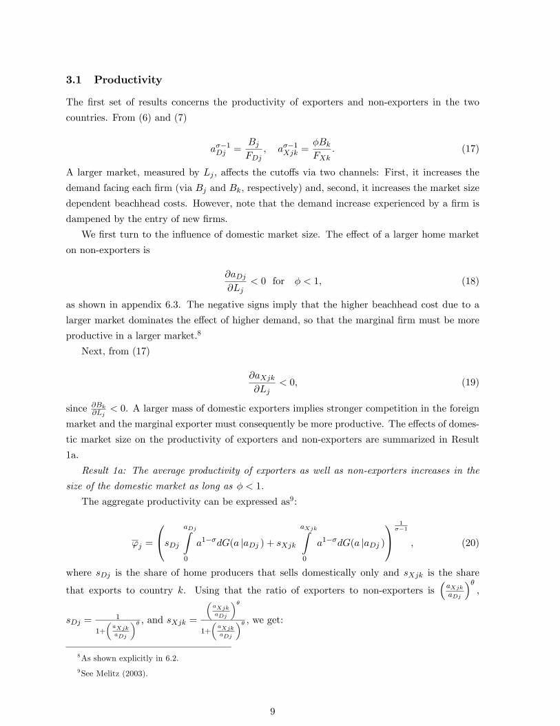
3.1 Productivity

The �rst set of results concerns the productivity of exporters and non-exporters in the two

countries. From (6) and (7)

a��1Dj =BjFDj

; a��1Xjk =�BkFXk

: (17)

A larger market, measured by Lj ; a¤ects the cuto¤s via two channels: First, it increases the

demand facing each �rm (via Bj and Bk, respectively) and, second, it increases the market size

dependent beachhead costs. However, note that the demand increase experienced by a �rm is

dampened by the entry of new �rms.

We �rst turn to the in�uence of domestic market size. The e¤ect of a larger home market

on non-exporters is

@aDj@Lj

< 0 for � < 1; (18)

as shown in appendix 6.3. The negative signs imply that the higher beachhead cost due to a

larger market dominates the e¤ect of higher demand, so that the marginal �rm must be more

productive in a larger market.8

Next, from (17)

@aXjk@Lj

< 0; (19)

since @Bk@Lj

< 0. A larger mass of domestic exporters implies stronger competition in the foreign

market and the marginal exporter must consequently be more productive. The e¤ects of domes-

tic market size on the productivity of exporters and non-exporters are summarized in Result

1a.

Result 1a: The average productivity of exporters as well as non-exporters increases in the

size of the domestic market as long as � < 1.

The aggregate productivity can be expressed as9:

'j =

0@sDj aDjZ0

a1��dG(a jaDj ) + sXjk

aXjkZ0

a1��dG(a jaDj )

1A1

��1

; (20)

where sDj is the share of home producers that sells domestically only and sXjk is the share

that exports to country k. Using that the ratio of exporters to non-exporters is�aXjkaDj

��;

sDj =1

1+

�aXjkaDj

�� ; and sXjk =�aXjkaDj

��1+

�aXjkaDj

�� , we get:

8As shown explicitly in 6.2.

9See Melitz (2003).

9

'j =1

aDj

��

� � � + 1

� 1��1

0B@1 +�aXjkaDj

�2�+1��1 +

�aXjkaDj

��1CA

1��1

: (21)

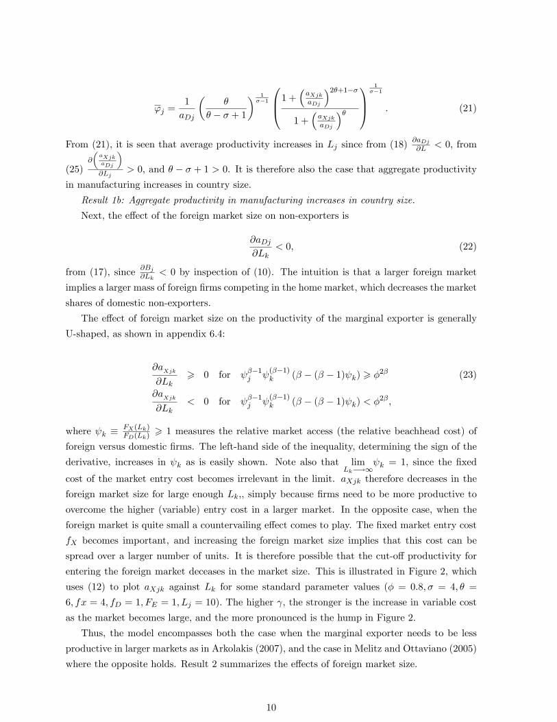
From (21), it is seen that average productivity increases in Lj since from (18) @aDj@L < 0, from

(25)@

�aXjkaDj

�@Lj

> 0, and � � � + 1 > 0. It is therefore also the case that aggregate productivity

in manufacturing increases in country size.

Result 1b: Aggregate productivity in manufacturing increases in country size.

Next, the e¤ect of the foreign market size on non-exporters is

@aDj@Lk

< 0; (22)

from (17), since @Bj@Lk

< 0 by inspection of (10). The intuition is that a larger foreign market

implies a larger mass of foreign �rms competing in the home market, which decreases the market

shares of domestic non-exporters.

The e¤ect of foreign market size on the productivity of the marginal exporter is generally

U-shaped, as shown in appendix 6.4:

@aXjk

@Lk> 0 for ��1j

(��1)k (� � (� � 1) k) > �2� (23)

@aXjk

@Lk< 0 for ��1j

(��1)k (� � (� � 1) k) < �2�;

where k �FX(Lk)FD(Lk)

> 1 measures the relative market access (the relative beachhead cost) of

foreign versus domestic �rms. The left-hand side of the inequality, determining the sign of the

derivative, increases in k as is easily shown. Note also that limLk�!1

k = 1; since the �xed

cost of the market entry cost becomes irrelevant in the limit. aXjk therefore decreases in the

foreign market size for large enough Lk;, simply because �rms need to be more productive to

overcome the higher (variable) entry cost in a larger market. In the opposite case, when the

foreign market is quite small a countervailing e¤ect comes to play. The �xed market entry cost

fX becomes important, and increasing the foreign market size implies that this cost can be

spread over a larger number of units. It is therefore possible that the cut-o¤ productivity for

entering the foreign market deceases in the market size. This is illustrated in Figure 2, which

uses (12) to plot aXjk against Lk for some standard parameter values (� = 0:8; � = 4; � =

6; fx = 4; fD = 1; FE = 1; Lj = 10): The higher , the stronger is the increase in variable cost

as the market becomes large, and the more pronounced is the hump in Figure 2.

Thus, the model encompasses both the case when the marginal exporter needs to be less

productive in larger markets as in Arkolakis (2007), and the case in Melitz and Ottaviano (2005)

where the opposite holds. Result 2 summarizes the e¤ects of foreign market size.

10

γ=1

γ=1.3

γ=0.7

Figure 2: Exporter cut-o¤ productivity in relation to foreign market size (� = 0:8; � = 4; � =

6; fX = 4; fD = 1; FE = 1; Lj = 10)

Result 2: The average productivity of non-exporters increases in the size of the foreign

market. The average productivity of exporters is generally U-shaped in the foreign market size.

Next using (11) and (12), the relative cut-o¤ productivity for non-exporters and exporters

in the home country is

�aDjaXjk

��=

FXkFDjk

�1� k1� j

�> 1; for

FXjj

> FDk 8 j; k; and j ;k < 1: (24)

There is strong empirical support for exporters being more productive than domestic �rms,

and as mentioned above, we follow Melitz (2003) by making parameter assumptions for this to

hold: FXjj

> FDk: Moreover, market size is also of importance for the relative productivity of

exporters as compared to non-exporters, in accordance with the stylized evidence presented in

Figure 3 in the introduction:

@�aDjaXjk

�@Lj

< 0 for j ;k < 1; (25)

as shown in appendix 6.6. The larger is the home country, the less productive are exporters as

compared to non-exporters. Essentially, the higher �xed cost associated with the larger home

market will push up the relative productivity of domestic �rms, which makes exporters look

less productive in comparison.

Result 3: Exporters are more productive than producers for the domestic market. However,

this e¤ect decreases in the size of the home country.

11

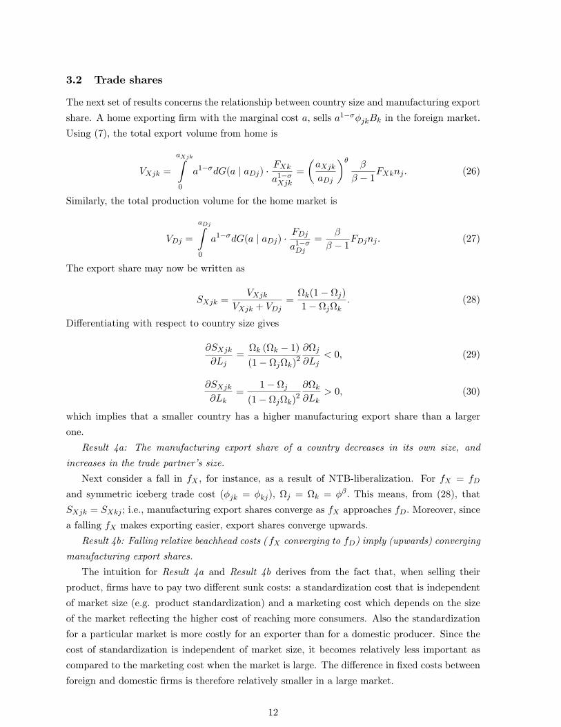
3.2 Trade shares

The next set of results concerns the relationship between country size and manufacturing export

share. A home exporting �rm with the marginal cost a; sells a1���jkBk in the foreign market.

Using (7), the total export volume from home is

VXjk =

aXjkZ0

a1��dG(a j aDj) �FXk

a1��Xjk

=

�aXjkaDj

�� �

� � 1FXknj : (26)

Similarly, the total production volume for the home market is

VDj =

aDjZ0

a1��dG(a j aDj) �FDj

a1��Dj

=�

� � 1FDjnj : (27)

The export share may now be written as

SXjk =VXjk

VXjk + VDj=k(1� j)1� jk

: (28)

Di¤erentiating with respect to country size gives

@SXjk@Lj

=k (k � 1)(1� jk)2

@j@Lj

< 0; (29)

@SXjk@Lk

=1� j

(1� jk)2@k@Lk

> 0; (30)

which implies that a smaller country has a higher manufacturing export share than a larger

one.

Result 4a: The manufacturing export share of a country decreases in its own size, and

increases in the trade partner�s size.

Next consider a fall in fX , for instance, as a result of NTB-liberalization. For fX = fD

and symmetric iceberg trade cost (�jk = �kj), j = k = �� : This means, from (28), that

SXjk = SXkj ; i.e., manufacturing export shares converge as fX approaches fD: Moreover, since

a falling fX makes exporting easier, export shares converge upwards.

Result 4b: Falling relative beachhead costs ( fX converging to fD) imply (upwards) converging

manufacturing export shares.

The intuition for Result 4a and Result 4b derives from the fact that, when selling their

product, �rms have to pay two di¤erent sunk costs: a standardization cost that is independent

of market size (e.g. product standardization) and a marketing cost which depends on the size

of the market re�ecting the higher cost of reaching more consumers. Also the standardization

for a particular market is more costly for an exporter than for a domestic producer. Since the

cost of standardization is independent of market size, it becomes relatively less important as

compared to the marketing cost when the market is large. The di¤erence in �xed costs between

foreign and domestic �rms is therefore relatively smaller in a large market.

12

For example, suppose that Sweden and the United States have similar levels of regulation

but di¤erent tastes in the design of labels, packages and instructions. Then, the cost of stan-

dardization is similar for an American �rm targeting the Swedish market and for a Swedish

�rm targeting the American market. However, the market size dependent marketing cost is

much higher for �rms selling in the US as compared to those selling in Sweden. The di¤erence

in �xed costs for Swedish exporters and American domestic producers, both serving the same

market, is therefore smaller in relative terms than the di¤erence between American exporters

and Swedish domestic producers. Consequently, the smaller country, i.e. Sweden, has a larger

share of manufacturing exports in its production.

Second, since Swedish exporters are more concerned with the larger marketing costs than the

standardization costs, as compared to American exporters to Sweden, it must be the case that

the decrease in standardization costs for foreign markets (fX approaching fD) a¤ects American

�rms more than Swedish �rms. This means that American �rms will increase their exports at

a greater pace than Swedish �rms and therefore, they will start catching up with their Swedish

counterparts. In the aggregate, the American export share of manufacturing production will

then approach the (larger) Swedish export share and export shares converge across countries.

In the extreme, when the cost of standardization is the same for the domestic and the foreign

market (fX = fD), export shares converge completely across countries.

It may be useful to compare our results to the standard models. Here, we use the Melitz

(2003) model with a homogenous good and freely traded A-sector à la Helpman, Melitz, and

Yeaple (2004). It is easily shown that the manufacturing export shares are independent of

country size in this model without our assumption of a market size dependent beachhead cost.

However, our result may also be compared to the standard Dixit-Stiglitz trade model without

a homogenous good A-sector (see e.g. Helpman (1987)). Like our model, trade shares are neg-

atively related to market size in that model. However, in contrast to our model, manufacturing

trade shares diverge as trade costs fall: trade shares increase from zero in autarky to the share

of the foreign market in total demand at free trade.10 As shown below in the empirical section,

we believe our prediction of converging manufacturing export shares to be supported by data.

3.3 The gravity equation

Our modi�cation of the Melitz model has implications for the gravity equation. Consider a

setting without the A-sector and with m countries indexed by j and k: The factory gate price

of each �rm is now pij =���1aiwj ; where wj is the factor price in country j: The export from j

to k is

Ejk = nj

��

� � 1� jkwjPk

�1��VjkYk; (31)

10Naturally, in this model there is no beachhead cost that can be a¤ected by trade liberalization.

13

where Vjk �aXjkR0

a1��i dG(a j aDj): The GDP of country j consists of the sum of sales in all

markets including itself:

Yj =

mXk=1

Ejk =

mXk=1

nj

��

� � 1� jkwjPk

�1��VjkYk: (32)

Following the methodology of Anderson and van Wincoop (2003), a gravity equation of trade

may be derived by solving (32) for nj�

���1wj

�1��and substituting the solution into (31). This

gives:

Ejk =YjYkY w

�1��jk Vjk

P 1��k

Pmj=1

��1��jk

P 1��k

�skVjk

; (33)

where sk � YkY w ; and Y

w �Pmj=1 Yj :

Solving the integral for Vjk gives

Vjk =�

� � � + 1

�aXjkaDj

��a1��Xjk: (34)

Using this and the fact that a1��Xjk =FXkP

1��k

�1��jk Yk; from the cut-o¤ conditions, gives the following

gravity equation

Ejk =YjYkY w

���jk

�YkFXk

� ���1�1

P��kPmk=1

��jkPk

���sk

�YkFXk

� ���1�1

: (35)

The expression may be compared to the standard Anderson and van Wincoop gravity formula-

tion: Ejk =YjYkY w

�1��jk

P��k

Pmk=1

��jkPk

�1��sk: The di¤erence is essentially the term

�YjFXj

� �+1����1

; which

multiplies the frictional trade cost.11 This term measures the importance of the exporters�

market entry cost in relation to the size of the export market, that is, trade resistance related

to the market entry cost. Note also that a higher � decreases the negative impact of FXj on

trade, as pointed out by Chaney (2008).

Finally, substituting (16) into (35) gives

Ejk =YjYkY w

���jk

�Yk

fX+L k

� ���1�1

P��kPmk=1

��jkPk

���sk

�Yk

fX+L k

� ���1�1

: (36)

11A further di¤erence as compared to the standard gravity equation is that our expression for multilateral

resistance, namelymXk=1

��jkPk

��ksk�

YkFXk

��+1����1

; does not equal Pj in our set-up. The reason for this is that the

exporters�market entry cost FXk depends on population size and is therefore not symmetric when there is trade

between two countries of di¤erent size.

14

This shows that our speci�cation gives a justi�cation for the common usage of GDP per capita

as explanatory variable in the gravity regression. GDP per capita enters because a higher

purchasing power per head makes it worth more to �rms to pay the entry cost, which increases

by heads. However, since the entry cost increases non-linearly in the size of the population, it isYk

fX+L krather than exactly GDP per capita that should enter the gravity regression according

to our model.

4 Empirical Section

We have derived a set of new results. We will here explicitly test only a few of them. For

the other results we will discuss to what extent they seem consistent with existing empirical

evidence. One obvious limitation is that several of our results ideally should be tested using a

cross country �rm level data set, and such a data set is not yet available.

Our �rst result that �rms on average are more productive in large markets is consistent

with several empirical studies showing that workers and �rms on average are more productive

in larger markets (Head and Mayer 2004, Redding and Venables 2004, Syverson 2004, 2006, and

Amiti and Cameron 2007), and we do not here perform any independent test of this. Likewise,

Result 2, that the productivity of exporters is U-shaped in the size of the export market is

consistent with both Arkolakis (2007) indicating that the productivity of exporters decreases in

the export market size, and with the opposite result in Melitz and Ottaviano (2005). Concerning

Result 3, that country size a¤ects the relative performance of exporters and non-exporters, we

turn to stylized evidence in the following section. Results 4a,b are explicitly tested in section

4.2. Finally our theoretical result that GDP per capita enters the gravity equation is consistent

with the common use of GDP per capita as control variable in empirical applications of the

gravity equation (e.g. Head, Mayer, and Ries (2008)).

4.1 Empirical evidence of Result 3

We turn to stylized evidence to evaluate Result 3 that country size a¤ects the relative perfor-

mance of exporters and non-exporters. A study by Schank, Schnabel, and Wagner (2007) o¤ers

a literature overview where they measure the wage premium of exporting �rms as compared

to non-exporting �rms. Typically, a regression is run on �rm level data with some measure

of wages as the dependent variable, and a dummy variable indicating whether the �rm is an

exporter. The estimated coe¢ cient for this dummy variable is the exporter wage premium as

compared to that of non-exporters. We interpret this wage premium to indicate productivity

di¤erences between exporters and non-exporters.12 Figure 3 plots the exporter wage premium

versus market size (population) of countries in the studies surveyed in the appendix of Schank,

12This interpretation is consistent with a non-competitive wage setting à la Shapiro and Stiglitz (1984) or by

learning e¤ects as in Malchow-Møller, Markusen, and Schjerning (2007).

15

­4­3

­2­1

01

log(

wag

e pr

emiu

m)

7 8 9 10 11 12log(population)

Source: Schank, Schnabel & Wagner (wp 2006) and Penn World Tables.

As in Schank, Schnabel & Wagner (wp 2006).Population and exporter wage premia

Figure 3: Export premiums decrease in country size.

Schnabel, and Wagner (2007).13 We have also added an observation for Sweden using data

provided by Statistics Sweden. Naturally, it must be acknowledged that all regressions are not

done with exactly the same methodology or fully comparable data. Nevertheless, Figure 3 shows

a negative correlation between the exporter wage premium and population size in accordance

with result 3. Running a regression on this data gives a slope of �0:58 with a t-value of �2:93.

4.2 Empirical evidence of Result 4a,b

In this section, we empirically test predictions of our model related to the e¤ects of market size on

trade shares. First, we check that our dataset has the well known property that manufacturing

export shares are negatively correlated with country size, as predicted by Result 4a. Even

though this is well known theoretical result, it does not typically apply in this type of model.

We employ sector level data within the OECD using the STAN database with yearly observations

from 1980 to 2003, and run the simple regression

sist = �0 + �1lit + "ist, (37)

where sist � log�XY ist

�; lit � logLit: The regression is run at the sectorial level. Table 1 shows

the regression of export shares over GDP on a sectorial level in 2001. The regression includes

�xed e¤ects for sectors. The coe¢ cient for population, which can be interpreted as a standard

elasticity, is highly signi�cant and of the expected sign.

13We use population to measure market size since it most closely corresponds to our model speci�cation.

However, the pattern of exporter wage premia to market size is the same, if GDP is instead used to measure

16

Year 2001

Dependent variable XY

(1)

lit -0.15���

(0.024)

Sector dummies Yes

Observations 595

R squared 0.43

The table reports the estimates of the regression of

export shares on country size controlling for sector-

speci�c �xed e¤ects. The export share is at the

sectoral level and population at the country level.

Note: Standard errors in parentheses. � signi�cant

at 10%, �� signi�cant at 5%, ��� signi�cant at 1%.

Table 1: Export Shares and Country Size

Next Result 4b states that the export share of the manufacturing sector across countries

converges as the �xed component of the exporting beachhead cost, fX , approaches the value for

the �xed component of the domestic beachhead cost, fD. Given that this has been happening

over time, we should observe converging manufacturing trade shares over time. The assumption

that the relative access cost to foreign markets, as compared to that of the domestic market,

has been falling over time is very much in line with the often cited e¤ect of globalization making

the world more alike. A concrete example supporting this assumption is the process of prod-

uct standardization and removal of non-tari¤ barriers to trade (NTB-liberalization) within the

European Union during the last 20-30 years. GATT and WTO negotiations have also aimed

at reducing nontari¤ barriers to trade during this period. Finally, the rapid improvement of

telecommunications, including the internet, simpli�es business contacts and information gath-

ering about foreign markets, which may be interpreted as a fall in fX :

We look at the evolution of manufacturing export shares over time, at a sectorial level within

the OECD using the STAN database with yearly observations from 1980 to 2003.14 Accepting

market size.

14We include all manufacturing sectors except those related to the extraction of raw materials since we do not

believe these to be a¤ected by the dynamics described in this paper.

17

.42

.44

.46

.48

.5C

oeffi

cien

t of v

aria

tion 

for e

xpor

t/gdp

1980 1985 1990 1995 2000year

1980­2000Coefficient of variation in manufacturing export shares

Figure 4: The coe¢ cient of variation for country level export shares. Source: OECD STAN.

the assumption that the process of falling access costs to foreign markets has occurred gradually

over time during the period investigated, we should observe converging manufacturing export

shares. First, we graphically explore the data on manufacturing aggregated to the country

level. We want a balanced panel so that we only include country and sector pairs that have

nonmissing data throughout the period 1980 to 2000, before we aggregate to the country level.

For this period, there are data on most sectors for most countries throughout. The appendix

contains a list of the 18 countries that are included. First, Figure 4 plots the evolution of the

coe¢ cient of variation of the distribution of trade shares (exports divided by output) for the

sample of countries. We use the coe¢ cient of variation since it is neutral to scale. The graph

gives an indication that the average dispersion of trade shares in manufacturing across countries

decreases throughout the period. This result is driven by the fact that the mean grows more

rapidly over time than the standard deviation. Figure 5 plots histograms of country level trade

shares for �ve equally spaced years in the period. It can be seen that the mean increases while

a change in the absolute level of dispersion is more di¢ cult to detect.

Next, we proceed to use sectorial data to analyse trade share convergence using a regression

framework from the standard empirical growth literature (see e.g. Barro and Sala-i-Martin

(1991), Barro and Sala-i-Martin (1992), Bernard and Jones (1996) and Mankiw, Romer, and

Weil (1992)). We use the initial value of the manufacturing export share for which we have

data and regress the average growth rate in export shares, f�sis; on the average growth rate ofpopulation and the initial level of trade shares, where the average growth rates are computed

as the coe¢ cient on the trend dummy in a regression of logged values on a constant and linear

trend, see e.g. Bernard and Jones (1996):

f�sis = �0 + �1sis0 + �2f�li + �3Ds + "is.

18

01

23

Freq

uenc

y

0 .1 .2 .3 .4 .5 .6 .7 .8 .9 1export/gdp

1980

01

23

Freq

uenc

y

0 .1 .2 .3 .4 .5 .6 .7 .8 .9 1export/gdp

1985

01

23

Freq

uenc

y

0 .1 .2 .3 .4 .5 .6 .7 .8 .9 1export/gdp

1990

01

23

Freq

uenc

y

0 .1 .2 .3 .4 .5 .6 .7 .8 .9 1export/gdp

1995

01

23

Freq

uenc

y

0 .1 .2 .3 .4 .5 .6 .7 .8 .9 1export/gdp

2000

Distribution of export shares across time

Figure 5: The mean country level export share. Source: OECD STAN Industrial Database.

We allow for arbitrary correlation of the error terms over time at the country level by

clustering of errors. Sector dummies are included. The model predicts that �1 should be

negative since the higher was the initial level, the lower would be the average change over time

if convergence held. In Table 2, it is shown that the growth rate of export shares depends

negatively on the initial level in 1980, thereby suggesting convergence within the OECD at the

sectorial level.

5 Conclusion

This paper has explicitly modelled a market size dependent market access or beachhead cost in

the heterogeneous �rms and trade model of Melitz (2003). We model this cost as having one

variable component that increases in market size, and one �xed component. The �xed compo-

nent could e.g. be interpreted as the cost of standardizing a product for a particular market,

while the variable cost term e.g. represents the fact that the advertising cost of introducing a

new product increases in the size of the market (the number of consumers).

In essence we make a relatively small change to the framework of Helpman, Melitz, and

Yeaple (2004), which preserves the analytical solvability of the model. Nevertheless it leads to a

number of new results. The productivity of non-exporting as well as exporting �rms will depend

on market size, as will manufacturing export shares. In particular, we show that �rms based in

a large market are more productive than �rms in a smaller market, due to the higher �xed costs

related to establishing a brand in these markets. The relationship between exporter productivity

and export market size is U-shaped, however. This is because a larger market means that the

�xed entry cost (e.g. standardization) can be spread over more units, while the variable entry

cost (advertising) increases in the market size. Therefore, for su¢ ciently small export markets,

19

Years 1980 to 2002

Dependent variable ]�sist

si;1980 -0.020���

(0.002)

Sector dummies Yes

Observations 406

R squared 0.37

The table reports the estimates from the convergence regression of the

average change of trade shares at the sectoral level on the initial

levels of trade shares. Sector-speci�c e¤ects are controlled for by

sectoral �xed e¤ets.

Note: Standard errors in parentheses. Errors are clustered at the

country level. � signi�cant at 10% �� signi�cant at 5%��� signi�cant at 1%.

Table 2: Convergence (Initial Values)

the productivity of exporters decreases in the export market size, which is consistent with

the feature of the �rm level data in Eaton, Kortum, and Kramarz (2005) that the number of

exporting �rms increases in the size of the export market. For su¢ ciently large exports markets,

on the contrary, exporter productivity increases in the export market size in accordance with

Melitz and Ottaviano (2005). Furthermore we �nd that, as in the standard model, exporters are

more productive than non-exporters, but this productivity premium decreases in the size of the

home country, which is consistent with the stylized facts presented in the paper. Fourth, we show

that the manufacturing export share of a country decreases in its own size, and increases in the

size of the trade partner. This e¤ect decreases as markets are integrated (in the sense that the

�xed beachhead cost of foreign markets declines). If market access costs into foreign markets

have been falling over time�as a consequence of globalisation�the model predicts converging

manufacturing export shares over time. This prognosis is supported in the empirical section

of the paper, where this hypothesis is tested using sector level OECD data from 1980 to 2003.

Finally, we derive a gravity equation from our set-up. This equation contains a measure of GDP

per capita, which implies that our set-up gives a theoretical rationale for the common practice

of including this variable in gravity regressions of trade �ows.

20

References

Amiti, M., and L. Cameron (2007): �Economic Geography andWages,�Review of Economics

and Statistics, 89(1), 15�29.

Anderson, J. E., and E. van Wincoop (2003): �Gravity with Gravitas: A Solution to the

Border Puzzle,�American Economic Review, 93(1), 170�192.

Arkolakis, C. (2007): �Market Access Costs and the New Consumer Margin in International

Trade,�Unpublished.

Aw, B., S. Chung, and M. Roberts (2000): �Productivity and Turnover in the Export

Market: Micro Evidence from Taiwan and South Korea,�World Bank Economic Review, 14.

Axtell, R. L. (2001): �Zipf Distribution of U.S. Firm Sizes,�Science, 293.

Barro, R. J., and X. Sala-i-Martin (1991): �Convergence Across States and Regions,�

Brookings Papers on Economic Activity, 1, 107�158.

(1992): �Convergence,�Journal of Political Economy, 100(2), 223�251.

Bernard, A. B., J. Eaton, J. B. Jensen, and S. Kortum (2003): �Plants and Productivity

in International Trade,�American Economic Review, 93(4), 1268�1290.

Bernard, A. B., and J. B. Jensen (1995): �Exporters, Jobs and Wages in U.S. Manufac-

turing, 1976-1987,�Brookings Papers on Economic Activity, Microeconomics.

(1999a): �Exceptional Exporter Performance: Cause, E¤ect, or Both?,� Journal of

International Economics, 47.

(1999b): �Exporting and Productivity: Importance of Reallocation,�NBER Working

Paper No. 7135.

Bernard, A. B., and C. I. Jones (1996): �Comparing Apples to Oranges: Productivity Con-

vergence and Measurement Across Industries and Countries,�American Economic Review,

86(5), 1216�1238.

Bernard, A. B., S. Redding, and P. K. Schott (2007): �Comparative Advantage and

Heterogeneous Firms,�Review of Economic Studies, 74, 31�66.

Buzzell, R., G. Bradley, and R. Sultan (1975): �Market Share - A Key to Pro�tability,�

Harvard Business Review, Jan-Feb.

Chaney, T. (2008): �Distorted Gravity: The Intensive and Extensive Margins of International

Trade,�American Economic Review, 98(4).

21

Clerides, S. K., S. Lach, and J. R. Tybout (1998): �Is Learning by Exporting Impor-

tant? Microdynamic Evidence from Colombia, Mexico and Morocco,�Quarterly Journal of

Economics, 113(3), 903�947.

Combes, P.-P., G. Duranton, L. Gobillon, D. Puga, and S. Roux (2008): �The pro-

ductivity advantages of large cities: Distinguishing agglomeration from �rm selection,�Un-

published.

Eaton, J., S. Kortum, and F. Kramarz (2004): �Dissecting Trade: Firms, Industries, and

Export Destinations,�NBER Working Paper No. 10344.

(2005): �An Anatomy of International Trade: Evidence from French Firms,� 2005

Meeting Papers 197, Society for Economic Dynamics.

Head, K., and T. Mayer (2004): �Market Potential and the Location of Japanese Firms in

the European Union,�Review of Economics and Statistics, 86, 959�972.

Head, K., T. Mayer, and J. Ries (2008): �The erosion of colonial trade linkages after

independence,�CEPR Discussion Paper No. 6951.

Helpman, E. (1987): �Imperfect Competition and International Trade: Evidence from Four-

teen Industrial Countries,�Journal of the Japanese and International Economies, pp. 62�81.

Helpman, E., M. J. Melitz, and S. R. Yeaple (2004): �Export versus FDI with Hetero-

geneous Firms,�American Economic Review, 94(1), 300�316.

Luttmer, E. G. J. (2007): �Selection, Growth, and the Size Distribution of Firms,�Quarterly

Journal of Economics, 122(3), 1103�1144.

Malchow-Møller, N., J. R. Markusen, and B. Schjerning (2007): �Foreign Firms,

Domestic Wages,�NBER Working Paper No. 13001.

Mankiw, G. N., D. Romer, and D. Weil (1992): �A Contribution to the Empirics of

Economic Growth,�Quarterly Journal of Economics, 107(2), 407�438.

Melitz, M. J. (2003): �The Impact of Trade on Intra-Industry Reallocations and Aggregate

Industry Productivity,�Econometrica, 71(6), 1695�1725.

Melitz, M. J., and G. I. P. Ottaviano (2005): �Market Size, Trade and Productivity,�

NBER Working Paper No. 11393.

Ottaviano, G. I. P., T. Tabuchi, and J.-F. Thisse (2002): �Agglomeration and Trade

Revisited,�International Economic Review, 43.

Redding, S., and A. J. Venables (2004): �Economic Geography and International Inequal-

ity,�Journal of International Economics, 62, 53�82.

22

Schank, T., C. Schnabel, and J. Wagner (2007): �Do exporters really pay higher wages?

First evidence from German linked employer-employee data,�Journal of International Eco-

nomics, 72, 52�74.

Shapiro, C., and J. Stiglitz (1984): �Equilibrium Unemployment as a Discipline Device,�

American Economic Review, 74.

Syverson, C. (2004): �Market Structure and Productivity: A Concrete Example,�Journal of

Political Economy, 112(6).

(2006): �Prices, Spatial Competition, and Heterogeneous Producers: An Empirical

Test,�NBER Working Paper No. 12231.

Tybout, J. R. (2003): �Plant- and Firm-level Evidence on �New�Trade Theories,�in Handbook

of International Trade, ed. by E. K. Choi, and J. Harrigan. Basil-Blackwell, Oxford.

Yeaple, S. (2005): �A Simple Model of Firm Heterogeneity, International Trade, and Wages,�

Journal of International Economics, 65(1), 1�20.

6 Appendix

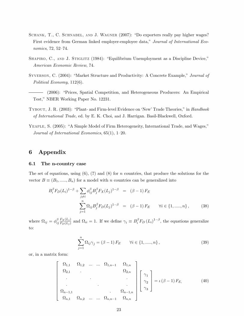
6.1 The n-country case

The set of equations, using (6), (7) and (8) for n countries, that produce the solutions for the

vector B � (B1; .....; Bn) for a model with n countries can be generalized into

B�i FD(Li)1�� +

Xj 6=i

��ijB�j FX(Lj)

1�� = (� � 1)FE

nXj=1

ijB�j FD(Lj)

1�� = (� � 1)FE 8i 2 f1; .....; ng ; (38)

where ij = ��ijFX(Lj)FD(Lj)

and ii = 1. If we de�ne i � B�i FD (Li)1��, the equations generalize

to:

nXj=1

ij j = (� � 1)FE 8i 2 f1; .....; ng , (39)

or, in a matrix form:26666666664

1;1 1;2 ::: ::: 1;n�1 1;n

2;1 : 2;n

: : :

: : :

n�1;1 : n�1;n

n;1 n;2 ::: ::: n;n�1 n;n

37777777775

2664 1

2

3

3775 = � (� � 1)FE; (40)

23

or

n�n n�1 = �n�1 (� � 1)FE (41)

where consists of entries where the element on the ith row and the jth column is ji, is a

vector� 1; 2; ..... ; n�1; n

�0 and � is an n dimensional vector of ones. Inverting the n�nmatrix yields the Bj which, in turn, determines the cut-o¤ productivity levels.

The case with three countries would then look as follows26641 12 13

21 1 23

31 32 1

37752664 1

2

3

3775 = � (� � 1)FE . (42)

The determinant of is

jj = 1 + 122331 +132132 � (�12 +�13 +�23) ; (43)

where �ij � ijji is the product of the bilateral trade costs between i and j. Solving the

system for gives:2664 1

2

3

3775 = 1

jj

26641��23 1332 � 12 1223 � 13

2331 � 21 1��13 1321 � 232132 � 31 1231 � 32 1��12

3775 � (� � 1)FE , (44)

which gives the following solutions for market size per �rm, Bi:

2664B1

B2

B3

3775 =(� � 1)FE

1 + 122331 +132132 � (�12 +�13 +�23)(45)

�

26641��23 +13 (32 � 1) + 12 (23 � 1)1��13 +23 (31 � 1) + 21 (13 � 1)1��12 +32 (21 � 1) + 31 (12 � 1)

37752664FD (L1)

��1

FD (L2)��1

FD (L3)��1

3775T

.

6.2 @@Lk

�aDjaDk

��> 0 for j;k < 1

Proof:

From (11)

�aDjaDk

��=FDkFDj

�1� k1� j

�.

Di¤erentiating w.r.t. Lk gives:

@

@Lk

�FDkFDj

�1� k1� j

��=

L �1k

FDj (1� j)

�1� k � (� � 1)k

�1�

1��1k �

�1��

��. (46)

24

The sign of the derivative depends on the sign of the term:�1� k � (� � 1)k

�1�

1��1k �

�1��

��. (47)

The �rst- and second-order conditions for a minimum of this term w.r.t. (Lk) are:

@

@k

�k

�1 + (� � 1)

�1�

1��1k �

�1��

���= �

�

1��1k �

�1�� � 1

�= 0

@2

@2k

�k

�1 + (� � 1)

�1�

1��1k �

�1��

���=

�

� � 11

��1�1k �

�1�� > 0: (48)

The minimum is, thus, given by k = 1 (since k = 1 () � = 1). Substituting k = 1

into (46) gives @@Lk

�aDjaDk

��= 0. Consequently, it must be the case that @

@Lk

�aDjaDk

��> 0 for

j ;k < 1.

6.3 @aDj@Lj

< 0

From (6.2), we have that

@�aDjaDk

�@Lk

=@aDj@Lk

1

aDk� aDj

(aDk)2

@aDk@Lk

> 0: (49)

Since from (11) @aDj@Lk< 0; (49) holds i¤ @aDk

@Lk< 0:

6.4@a

Xjk

@Lk

From (12)

a�Xjk =(� � 1)kFE

FXk

�(1� j)1� jk

�= (� � 1)FE(1� j)

1

FXk(1k� j)

: (50)

The sign of@a

Xjk

@Lkis therefore determined by the sign of

@

@Lk[FXk(

1

k� j)] (51)

=@

@Lk[F �XkF

1��Dk ��� � FXkj ]: (52)

Now

@

@Lk[F �XkF

1��Dk ��� � FXkj ] 7 0

,�FXkFDk

�� ��FDkFXk

� (� � 1)�

7 j��

,

� � FXkFDk

(� � 1) 7 jk:

25

6.5�aDjaDk

��> 1 i¤ Lk > Lj for j;k < 1

Proof:

First

Lj = Lk ()�aDjaDk

��=FDkFDj

�1� k1� j

�= 1:

That Lj = Lk ()�aDjaDk

��> 1 for j ;k < 1 now follows from @

@Lk

�aDjaDk

��> 0 for

j ;k < 1:

6.6@

�aDjaXjk

�@Lj

< 0 for j < 1.

Proof:

@

@Lj

�aDjaXjk

��= L �1j

FXkF 2Dj

(1� k)k (1� j)

0@(� � 1) j�1� FDj

FXk

�(1� j)

� 1

1A . (53)

The sign of (53) will depend on the sign of the term:

�j �

0@(� � 1)j�1� FDj

FXj

�(1� j)

� 1

1A : (54)

The F.O.C. when maximising �j w.r.t. � is:

(� � 1)�j�1� FDj

FXj

�� (1� j)

�(� � 1)�2j

�1� FDj

FXj

�� (1� j)2

= 0() 1� j(1� j)

= 0: (55)

So the only stationary point is j = 1. Furthermore, �j(j = 0) = �1 and lim(Lj)!1

�j = 0:

Therefore, it follows that for j 2 [0; 1):

d

dLj

�aDjaXjk

��< 0.

6.7 Countries included in Figure 5.

The following countries are included in Figure 5. This is a subset of the full STAN sample but

it is the only set of countries for which there is data for the full length of 1970 until 2002.

Austria

Belgium

Canada

Denmark

Finland

France

26

Iceland

Ireland

Italy

Japan

Netherlands

New Zealand

Norway

Portugal

Spain

Sweden

United Kingdom

United States

27