1

Chapter 3. Boundary-Value Problems in Electrostatics:

Spherical and Cylindrical Geometries

3.1 Laplace Equation in Spherical Coordinates

The spherical coordinate system is probably the most useful of all coordinate systems in study

of electrostatics, particularly at the microscopic level. In spherical coordinates , the

Laplace equation reads:

(

)

(

)

Try separation of variables . Then Eq. 3.1 becomes

[

(

)]

[

(

)

]

Since each side must be equal to a constant, , we get two equations.

Radial equation

(

)

Introducing , we obtain

The general solution of this equation is

Angular equation

(

)

We solve Eq. 3.6 using the separation of variable method again: . Then we

obtain two ordinary differential equations for and :

(3.1)

(3.2)

(3.3)

(3.4)

(3.5)

(3.6)

2

(

) [

]

Equation 3.8 has solutions

If the full azimuthal range is allowed, so that must be an

integer. The functions form a complete set of orthogonal functions on the interval

, which is nothing but a basis for Fourier series. The orthogonality relation is

∫

∫

Simultaneously, the completeness relation is

∑

∑

Associated Legendre Polynomials

Equation 3.7 can be written in terms of :

[

] [

]

This is the differential equation for the associated Legendre polynomials. Physically acceptable

solution (i.e., ) is obtained only if is a positive integer or 0. The solution is then

associated Legendre polynomial where and .

has the form,

| |

times a polynomial of order | |, which can be obtained by

Rodrigues formula,

| |

for

and the parity relation

| |

The orthogonal relation of the functions is expressed as

(3.7)

(3.8)

(3.9)

(3.12)

(3.13)

(3.14)

(3.10)

(3.11)

3

∫

(

)

| |

| |

The functions for are called Legendre polynomials which are the solutions when

the problem has azimuthal symmetry so that is independent of . The first few are

, ,

, …

The Legendre polynomials form a complete orthogonal set of functions on the interval

. The orthogonality condition can be written as

∫

and the completeness relation is expressed as

∑

Spherical Harmonics

The angular function can be written as , where is

normalization constant. The normalized angular functions,

√

for

are called spherical harmonics.

is either even or odd, depending on , i.e., :

In the spherical coordinate, corresponds to , therefore

√

√

The first few spherical harmonics are

(3.19)

(3.15)

(3.20)

(3.21)

(3.16)

(3.17)

(3.18)

4

√ , √

, √

, ….

Spherical harmonics form an orthonormal basis for and :

∫

The corresponding completeness relation is written as

∑ ∑

General Solution

The general solution for a boundary-value problem in spherical coordinates can be written as

∑ ∑ [ ]

3.2 Boundary-Value Problems with Azimuthal Symmetry

We consider physical situations with complete rotational symmetry about the z-axis (azimuthal

symmetry or axial symmetry). This means that the general solution is independent of , i.e.,

in Eq. 3.25:

∑[

]

The coefficients and can be determined by the boundary conditions.

Spherical Shell

Suppose that the potential is specified on the surface of a spherical shell of radius .

Inside the shell, for all because the potential at origin must be finite. The boundary

condition at leads to

∑

Using the orthogonality relation Eq. 3.17, we can evaluate the coefficients ,

∫

(3.23)

(3.25)

(3.26)

(3.27)

(3.28)

(3.22)

(3.24)

5

On the other hand, outside the shell, for all because the potential for must be

finite and the boundary condition gives rise to

∫

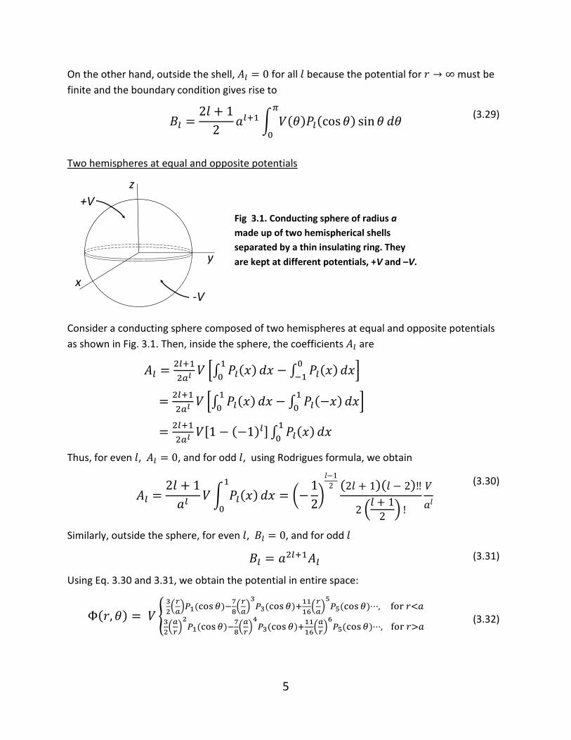
Two hemispheres at equal and opposite potentials

Consider a conducting sphere composed of two hemispheres at equal and opposite potentials

as shown in Fig. 3.1. Then, inside the sphere, the coefficients are

[∫

∫

]

[∫

∫

]

[ ] ∫

Thus, for even , , and for odd , using Rodrigues formula, we obtain

∫

(

)

(

)

Similarly, outside the sphere, for even , , and for odd

Using Eq. 3.30 and 3.31, we obtain the potential in entire space:

{

(

)

(

)

(

)

(

)

(

)

(

)

z

x

y

+V

-V

Fig 3.1. Conducting sphere of radius a

made up of two hemispherical shells

separated by a thin insulating ring. They

are kept at different potentials, +V and –V.

(3.29)

(3.30)

(3.31)

(3.32)

6

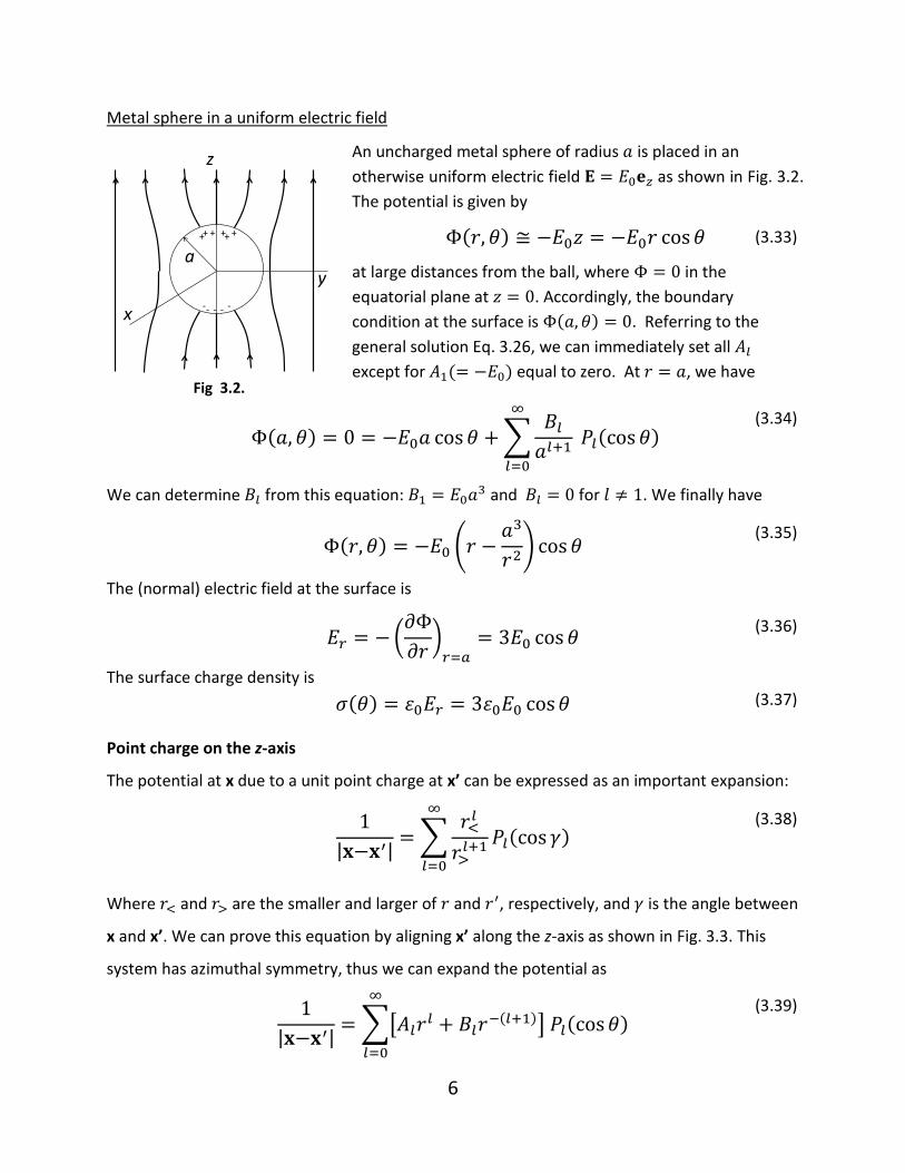
Metal sphere in a uniform electric field

An uncharged metal sphere of radius is placed in an

otherwise uniform electric field as shown in Fig. 3.2.

The potential is given by

at large distances from the ball, where in the

equatorial plane at . Accordingly, the boundary

condition at the surface is . Referring to the

general solution Eq. 3.26, we can immediately set all

except for equal to zero. At , we have

∑

We can determine from this equation: and for . We finally have

(

)

The (normal) electric field at the surface is

(

)

The surface charge density is

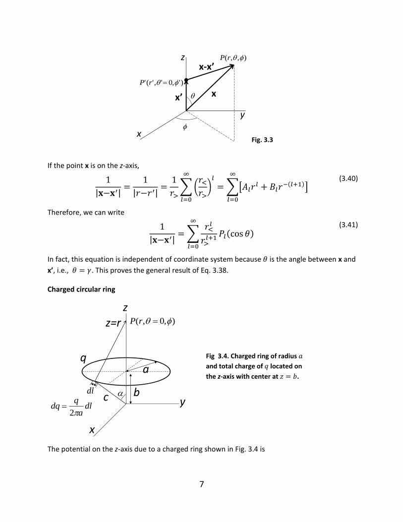
Point charge on the z-axis

The potential at x due to a unit point charge at x’ can be expressed as an important expansion:

| | ∑

Where and are the smaller and larger of and , respectively, and is the angle between

x and x’. We can prove this equation by aligning x’ along the z-axis as shown in Fig. 3.3. This

system has azimuthal symmetry, thus we can expand the potential as

| | ∑[

]

(3.33)

Fig 3.2.

(3.34)

(3.35)

(3.36)

(3.37)

(3.38)

(3.39)

z

x

y

+ +++ ++

- -- --

a

7

Fig. 3.3

If the point x is on the z-axis,

| |

| |

∑(

)

∑[

]

Therefore, we can write

| | ∑

In fact, this equation is independent of coordinate system because is the angle between x and

x’, i.e., . This proves the general result of Eq. 3.38.

Charged circular ring

The potential on the z-axis due to a charged ring shown in Fig. 3.4 is

z

x

y

x’ xq

f

),,( fqrP

)',0','(' fq rP

x-x’

z

x

y

),0,( fq rP

bc

z=r

aq

dla

qdq

2

dl

(3.40)

(3.41)

Fig 3.4. Charged ring of radius

and total charge of located on

the z-axis with center at .

8

∫

(3.42)

where and

. We can expand Eq. 3.42 using Eq. 3.38.

{∑

∑

Thus the potential at any point in space is

{∑

∑

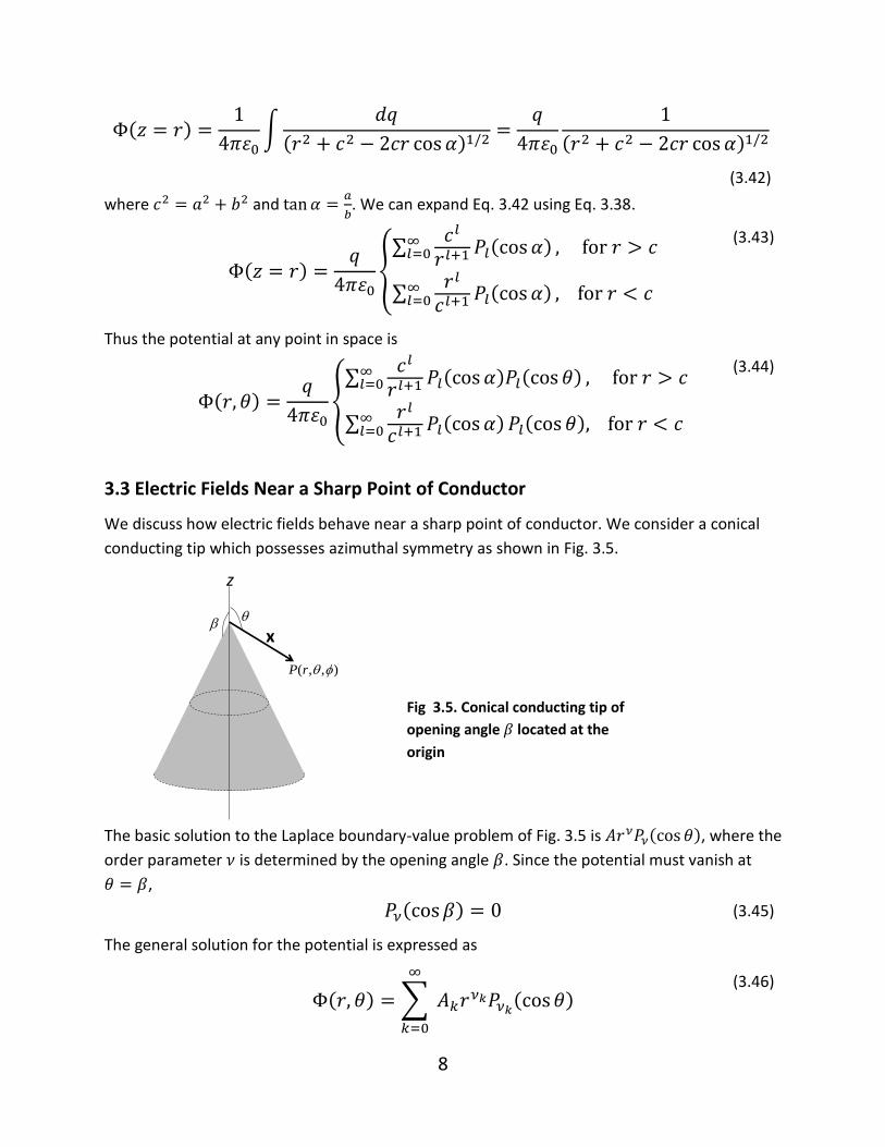
3.3 Electric Fields Near a Sharp Point of Conductor

We discuss how electric fields behave near a sharp point of conductor. We consider a conical

conducting tip which possesses azimuthal symmetry as shown in Fig. 3.5.

The basic solution to the Laplace boundary-value problem of Fig. 3.5 is , where the

order parameter is determined by the opening angle . Since the potential must vanish at

,

The general solution for the potential is expressed as

∑

z

),,( fqrP

x

q

(3.43)

(3.44)

Fig 3.5. Conical conducting tip of

opening angle located at the

origin

(3.45)

(3.46)

9

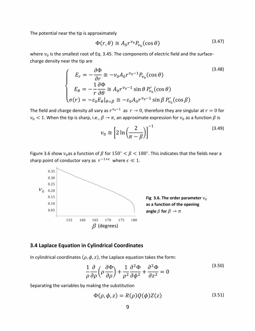
The potential near the tip is approximately

where is the smallest root of Eq. 3.45. The components of electric field and the surface-

charge density near the tip are

{

|

The field and charge density all vary as as , therefore they are singular at for

. When the tip is sharp, i.e., , an approximate expression for as a function is

[ (

)]

Figure 3.6 show as a function of for . This indicates that the fields near a

sharp point of conductor vary as where .

3.4 Laplace Equation in Cylindrical Coordinates

In cylindrical coordinates , the Laplace equation takes the form:

(

)

Separating the variables by making the substitution

155 160 165 170 175 180

0.05

0.10

0.15

0.20

0.25

0.30

0.35

(degrees)

0

(3.47)

(3.48)

Fig 3.6. The order parameter

as a function of the opening

angle for

(3.49)

(3.51)

(3.50)

10

Then we obtain the three ordinary differential equations:

(

)

The solutions of the first two equations are easily obtained:

and

When the full azimuthal angle is allowed, i.e., , must be an integer. We rewrite

the radial equation (Eq. 3.54) by chaning the variable .

(

)

The solutioins to this equation are best rexpressed as a power series in . There are two

independet solutions, and , called Bessel functions of the first kind and Neumann

functions, respectively. The Bessel function is defined as

(

)

∑

(

)

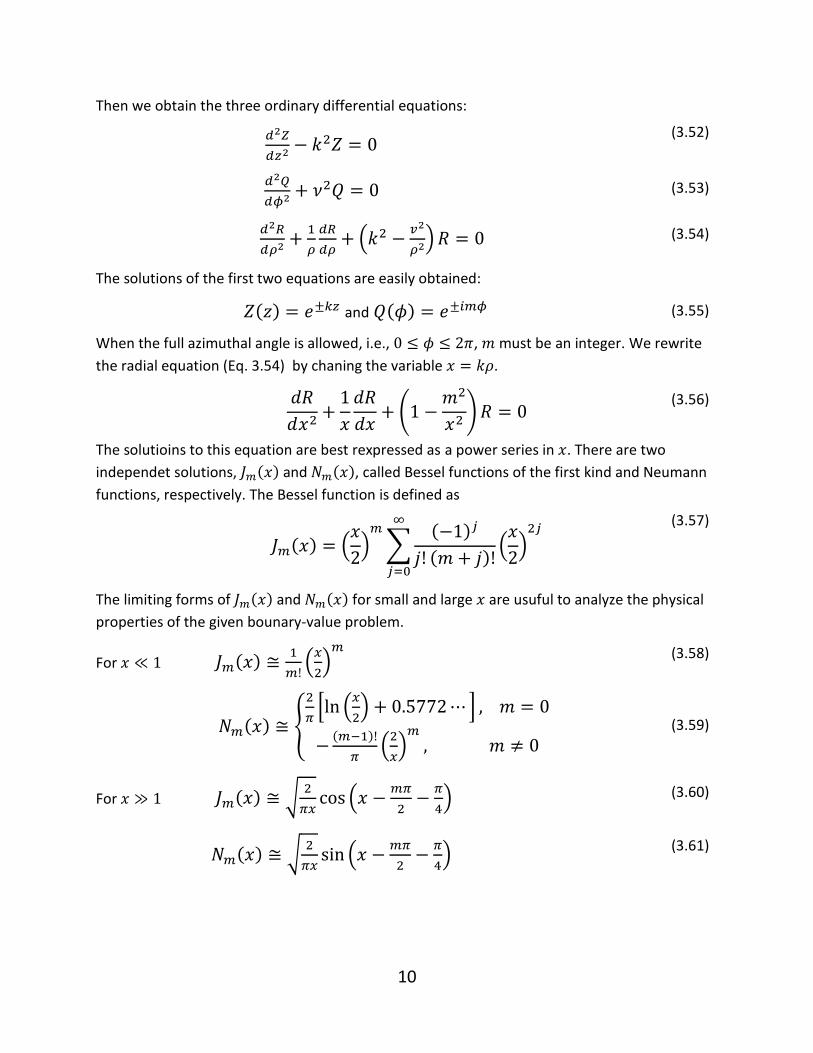
The limiting forms of and for small and large are usuful to analyze the physical

properties of the given bounary-value problem.

For

(

)

{

[ (

) ]

(

)

For √

(

)

√

(

)

(3.52)

(3.53)

(3.54)

(3.55)

)

(3.56)

(3.57)

(3.58)

(3.59)

(3.60)

(3.61)

11

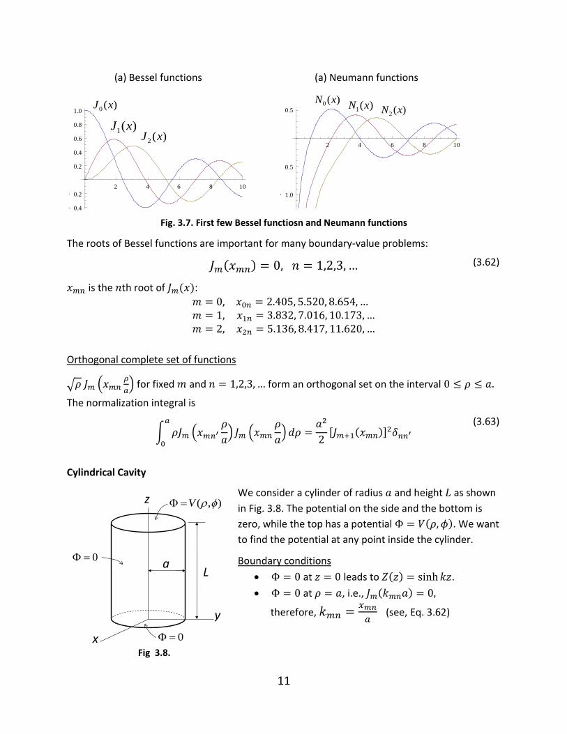
Fig. 3.7. First few Bessel functiosn and Neumann functions

The roots of Bessel functions are important for many boundary-value problems:

is the th root of :

Orthogonal complete set of functions

√ (

) for fixed and form an orthogonal set on the interval

The normalization integral is

∫ (

) (

)

[ ]

Cylindrical Cavity

We consider a cylinder of radius and height as shown

in Fig. 3.8. The potential on the side and the bottom is

zero, while the top has a potential . We want

to find the potential at any point inside the cylinder.

Boundary conditions

at leads to .

at , i.e.,

therefore,

(see, Eq. 3.62)

2 4 6 8 10

0.4

0.2

0.2

0.4

0.6

0.8

1.0

2 4 6 8 10

1.0

0.5

0.5)(0 xJ

)(1 xJ)(2 xJ

)(0 xN)(1 xN )(2 xN

(a) Bessel functions (a) Neumann functions

(3.62)

Fig 3.8.

(3.63)

z

x

y

La

0

0

),( fV

12

Then, the general solution can be expressed as

∑ ∑

(3.64)

At , we have , thus

∑ ∑

(3.65)

We can determine the coefficients and using the orthogol relations of the sinusoidal

and Bessel functions (see Eq. 3.63).

{

}

∫

∫

{

}

(3.66)

3.5 Poisson Equation and Green Functions in Spherical Coordinates

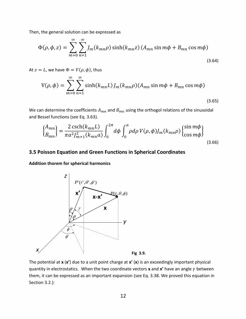
Addition thorem for spherical harmonics

Fig 3.9.

The potential at x (x’) due to a unit point charge at x’ (x) is an exceedingly important physical

quantity in electrostatics. When the two coordinate vectors x and x’ have an angle between

them, it can be expressed as an important expansion (see Eq. 3.38. We proved this equation in

Section 3.2.):

z

x

q

'q

x’ ),,( fqrP

)',','(' fqrP

x

yf

'f

x-x’

13

| | ∑

where and are the smaller and larger of and , respectively. It is of great interest and

use to express this equation in spherical coordiantes. The addition theorem of spherical

harmonics is an useful mathematical result for this purpose.

The addition theorem expresses a Legendre polynomial of order in the angle In spherical

coordiates as shown in Fig. 3.9:

∑

Combining Eq. 3.32 and 3.67, we obtain a completely factorized form in the coordinates x and

x’.

| | ∑

∑

We immediately see that Eq. 3.68 is the expansion of the Green function in spherical

coordinates for the case of no boundary surfaces, except at infinity.

Green function with a spherical boundary

The Green function appropriate for Dirichlet boundary conditions on the sphere of radius a

satisfies the equation (see Eq. 1.27)

and is expressed as (see Eq. 2.13 and 2.14)

( ) ( )

| | ( ) (2.13)

where for and for . The discussion of the

conducting sphere with the method of images indicates that the Green function can take the

form

( )

| |

|

|

Using Eq. 3.68 we rewrite Eq. 2.14 as

( ) ∑

[

(

)

] ∑

( )

(3.38)

(3.67)

1)

(3.68)

(2.14)

(3.69)

(1.27)

14

The radial factors inside and outside the sphere can be separately expressed as

(

)

{

(

)

(

)

General structure of Green function in spherical coordinates

The Green function appropriate for Dirichlet boundary conditions satisfies the equation (see Eq.

1.27)

In spherical coordinates the delta function can be written

Using the completeness relation for spherical harmonics (Eq. 3.24), we obtain

∑ ∑

Equation 1.27 and 3.72 leads to the expansion of the Green function

∑ ∑

and the equation for the radial Green function

[

]

The general solution of this equation for (see Eq. 3.5) can be written as

{

The coefficients A, B, A’, B’ are functions of r’ to be determined by the boundary conditions, the

discontinuity at , and the symmetry of

.

(3.70)

(3.71)

(3.72)

(1.27)

(3.73)

(3.75)

(3.74)

15

Green function with noboundary

For the case of no boundary, must be finite for and , therefore and are zero.

{

Then, the symmetry of of

leads to

where and are the smaller and larger of and , respectively. We determine the constant

using the discontinuity at . Integrating the radial equation 3.74 over the infinitesimally

narrow interval from to with very small , we obtain

[

]|

Substituning Eq. 3.77 into Eq. 3.78, we find

( )

This reduces to Eq. 3.68

| | ∑

∑

Green function with two concentric spheres

Suppose that the boundary surfaces are concentric spheres at and . on

the surfaces gives rise to

{

(

)

(

)

The symmetry of of

requires

(

)(

)

(3.76)

(3.77)

(3.78)

(3.79)

(3.68)

(3.80)

(3.81)

16

Using the discontinuity at (Eq. 3.78), we obtain the constant :

[ (

)

]

Combining Eq. 3.73, 3.81, and 3.82, we find the expansion of the Green function

∑ ∑

[ (

)

](

)(

)

(3.83)

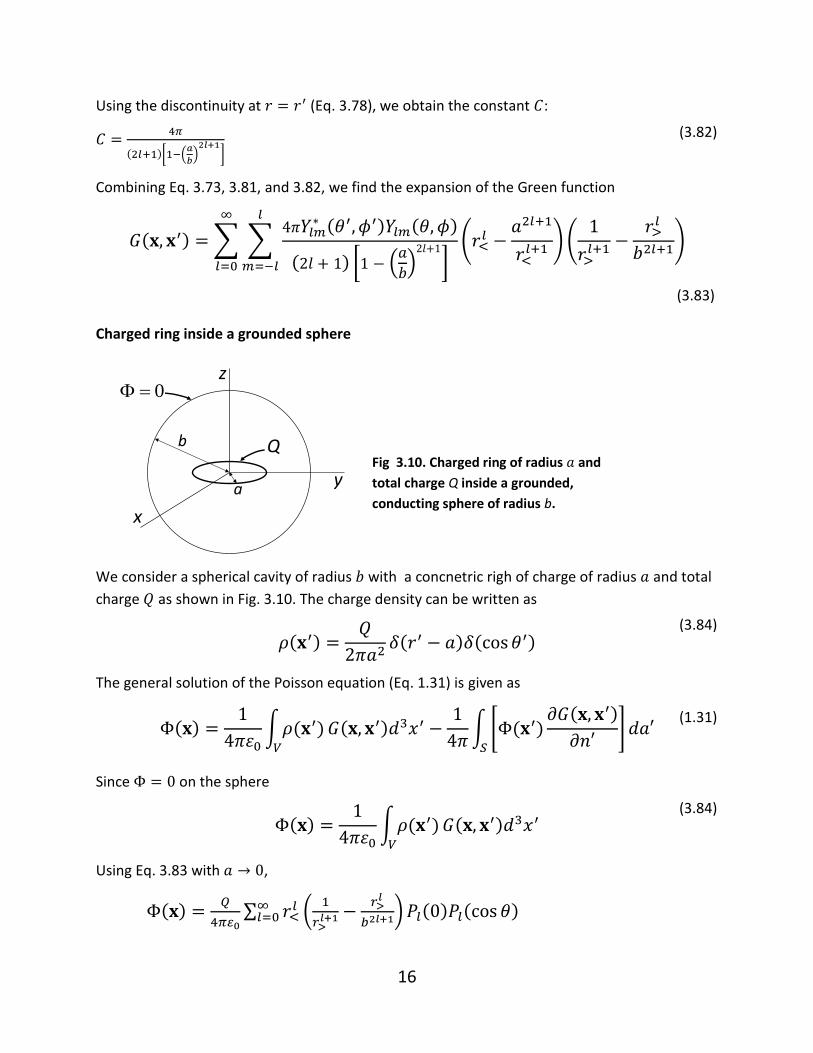
Charged ring inside a grounded sphere

We consider a spherical cavity of radius with a concnetric righ of charge of radius and total

charge as shown in Fig. 3.10. The charge density can be written as

The general solution of the Poisson equation (Eq. 1.31) is given as

∫

∫ [

]

Since on the sphere

∫

Using Eq. 3.83 with ,

∑

(

)

z

x

y

0

Q

a

b

(3.82)

Fig 3.10. Charged ring of radius and

total charge Q inside a grounded,

conducting sphere of radius b.

(1.31)

(3.84)

(3.84)

17

∑

(

)

where and are the smaller and larger of and , respectively.

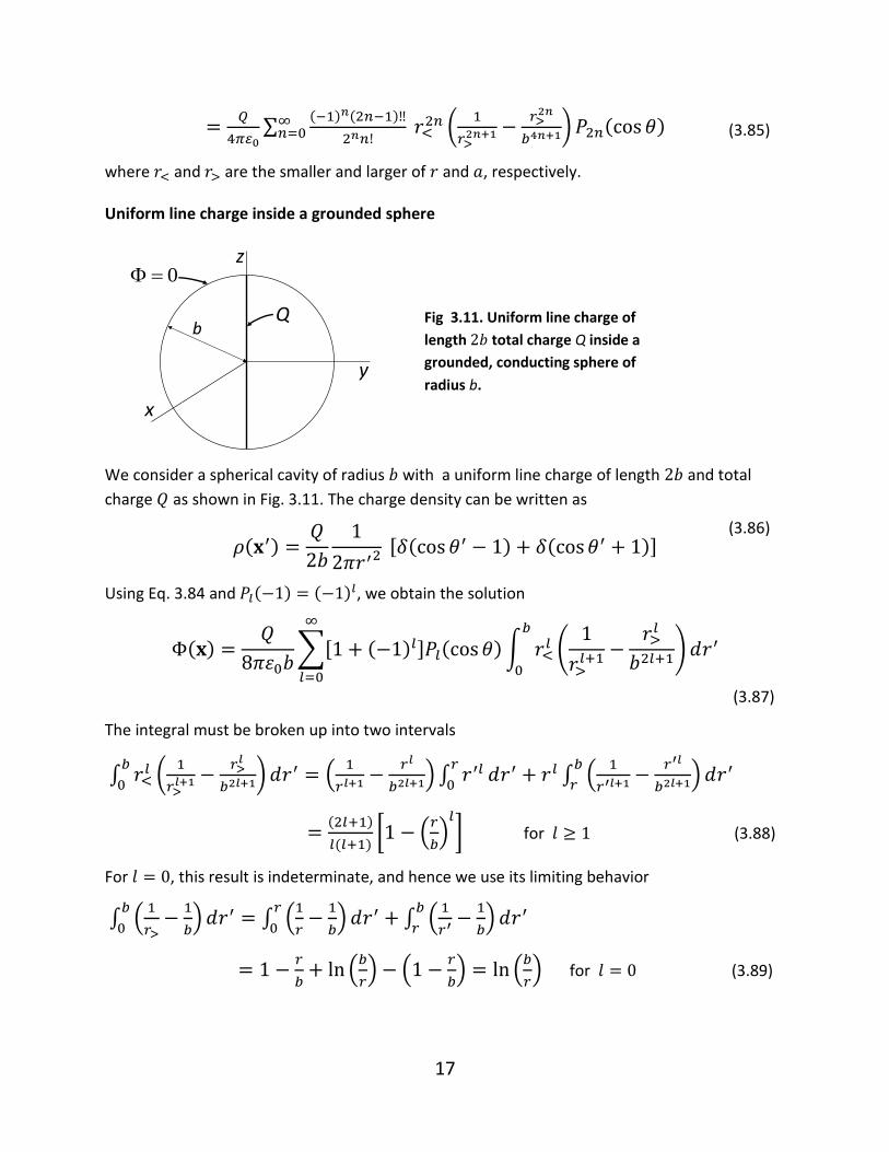
Uniform line charge inside a grounded sphere

We consider a spherical cavity of radius with a uniform line charge of length and total

charge as shown in Fig. 3.11. The charge density can be written as

[ ]

Using Eq. 3.84 and , we obtain the solution

∑[ ] ∫

(

)

(3.87)

The integral must be broken up into two intervals

∫ (

)

(

) ∫

∫ (

)

[ (

)

] for (3.88)

For , this result is indeterminate, and hence we use its limiting behavior

∫ (

)

∫ (

)

∫ (

)

(

) (

) (

) for (3.89)

z

x

y

0

Qb

(3.85)

Fig 3.11. Uniform line charge of

length total charge Q inside a

grounded, conducting sphere of

radius b.

(3.86)

18

Substituting Eq. 3.88 and 3.98 into Eq. 3.87, we find

{ (

) ∑

[ (

)

] } (3.90)

The surface charge density on the grounded sphere is

|

[ ∑

]

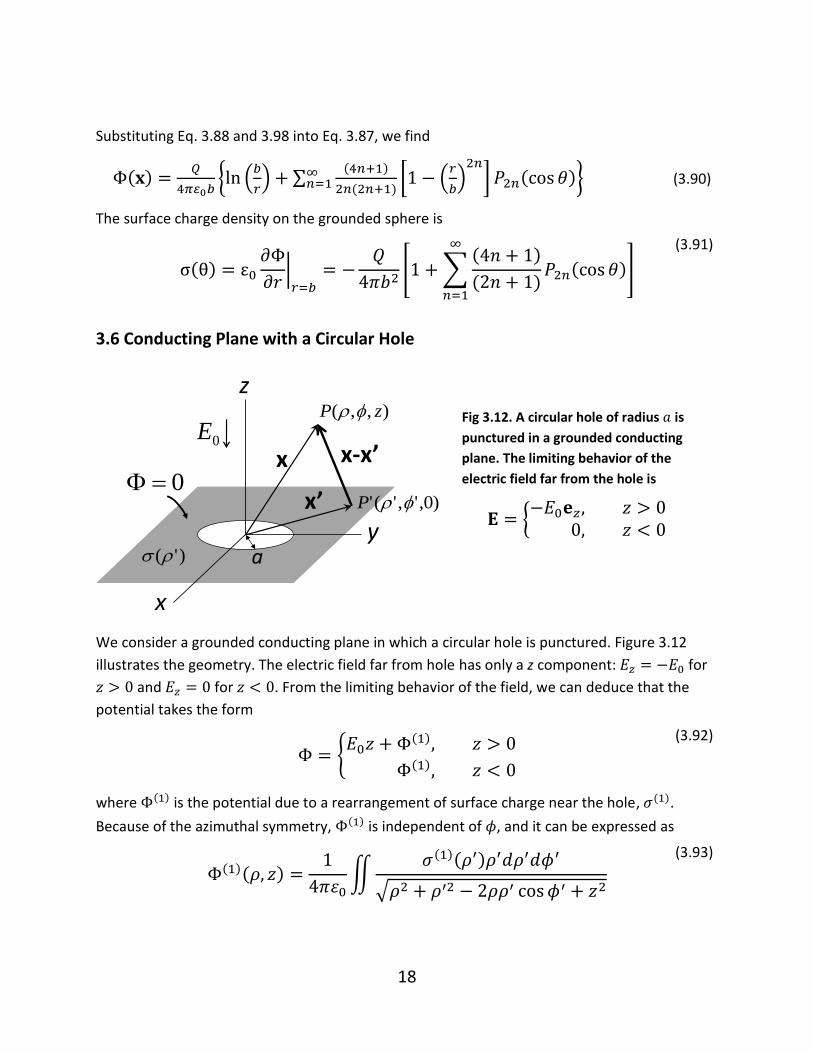
3.6 Conducting Plane with a Circular Hole

We consider a grounded conducting plane in which a circular hole is punctured. Figure 3.12

illustrates the geometry. The electric field far from hole has only a z component: for

and for . From the limiting behavior of the field, we can deduce that the

potential takes the form

{

where is the potential due to a rearrangement of surface charge near the hole, .

Because of the azimuthal symmetry, is independent of , and it can be expressed as

∬

√

z

x

y

0

a

0E),,( zP f

)0,','(' fP

x

x’

x-x’

)'(

(3.91)

{

Fig 3.12. A circular hole of radius is

punctured in a grounded conducting

plane. The limiting behavior of the

electric field far from the hole is

(3.92)

(3.93)

19

Mixed boundary conditions

is even in z, and hence

is odd. Since the total z component of electric field must be

continuous across in the hole, we must have (for )

|

|

Since

is odd,

|

|

This relation and the ground potential of the conducting surface complete the boundary

conditions for the entire xy plane. We therefore have mixed boundary conditions

{

|

|

Solution of Laplace equation in cylindrical coordinates

The general solution of the Laplace equation in cylindrical coordiates (see Eq. 3.51, 3.55 and

3.57) is

Because of the azimuthal symmetry, is independent of , and hence . Therefore,

can be written in terms of cylindrical coordinates

∫ | |

Boundary conditions and integral equatoins

The boundary conditions (Eq. 3.96) for the general solution (Eq. 3.98) give rise to the integral

equatoins of the coefficient :

{

∫

∫

There exists an analytic solution of these interal equations.

(

)

where is the spherical Bessel function of order 1.

(3.94)

(3.95)

(3.96)

(3.97)

(3.98)

(3.99)

(3.100)

20

Multipole expansion in the far-field region

In the far-feld region, i.e., in the region for | | and/or , the integral in Eq. 3.98 is mainly

determined by the contributions around , more precisely, for

. The expansion of

for small takes the form

[

]

The leading term gives rise to the asymptotic potential

∫ | |

| |∫ | |

| |(

√ )

| |

Here we have the asymptotic potential

| |

falling off with distance as and having an effective electric dipole moment,

where – for and for .

Potential in the near-field region

The potential in the neighborhood of the hole must be calculated from the exact expression

∫

| |

An integration by parts and Laplace transforms results in

[√

| |

(√

)]

where

√

(3.106)

(3.101)

(3.102)

(3.103)

(3.104)

(3.105)

21

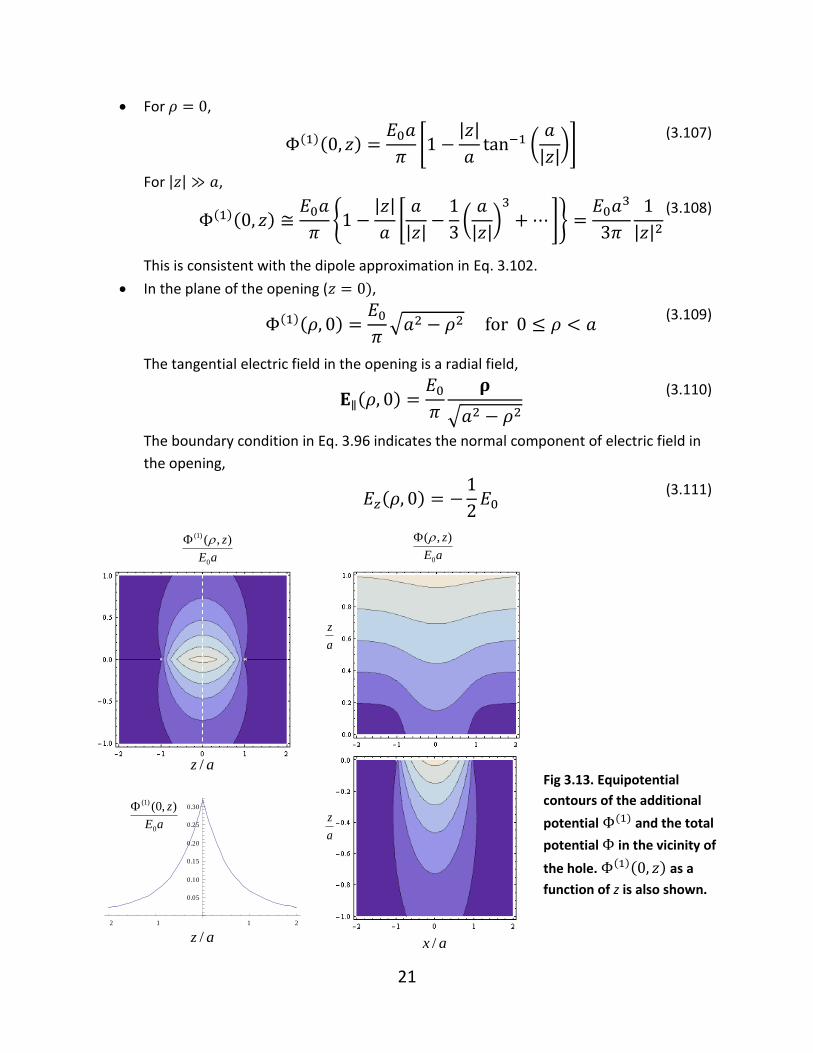
For ,

[

| |

(

| |)]

For | | ,

{

| |

[

| |

(

| |)

]}

| |

This is consistent with the dipole approximation in Eq. 3.102.

In the plane of the opening ( ,

√

The tangential electric field in the opening is a radial field,

√

The boundary condition in Eq. 3.96 indicates the normal component of electric field in

the opening,

az /

2 1 1 2

0.05

0.10

0.15

0.20

0.25

0.30

aE

z

0

)1( ),0(

az /

a

z

a

z

ax /

aE

z

0

)1( ),(

aE

z

0

),(

(3.107)

(3.108)

(3.109)

(3.110)

(3.111)

Fig 3.13. Equipotential

contours of the additional

potential and the total

potential in the vicinity of

the hole. as a

function of z is also shown.