U.S. DEPARTMENT OF THE INTERIOR

U.S. GEOLOGICAL SURVEY

Landform Classification of New Mexico by Computer

by

Richard Dikau 1 , Earl E. Brabb2 , and Robert M. Mark2

Open-File Report 91-634

Note: The shaded relief map, Plate 2 in this report, is a degraded image from an original 24 inch by 30 inch negative. A better quality contact photographic print is available for $58 each (price subject to change without notice) by sending a check payable to C-L Custom Photo Co., c/o U.S. Geological Survey Photo Library, Mail stop 914, Box 25046, Federal Center, Denver, CO 80225 (tel. 303-236-1010).

This report is preliminary and has not been reviewed for conformity with Geological Survey editorial standards or with the North American Statigraphic Code. Any use of trade, product, or firm names is for descriptive purposes only and does not imply endorsement by the U.S. Government.

1 Heidelberg University, Germany 2 USGS, Menlo Park, CA

LANDFORM CLASSIFICATION OF NEW MEXICO BY COMPUTER

by

Richard Dikau, Earl E. Brabb, and Robert M. Mark

INTRODUCTION

A project to understand the distribution, kind, and extent of landslide processes in New Mexico was begun in 1987 as part of a cooperative agreement between the U.S. Geological Survey (USGS), Institute di Ricerca per la Protezione Idrogeologica (IRPI) of the Italian National Research Council, the New Mexico Bureau of Mines and Mineral Resources, and the New Mexico Highway Department. New Mexico was chosen because of the joint interest of scientists and engineers in these agencies, because of the paucity of information about landslide processes in areas with arid and semi-arid climate, and because aerial photographs to study landslide processes are available for the entire State. The investigation was intended to cover all New Mexico in 2 years with only 3 people (Guzzetti, Brabb and Mark) and very limited research funds.

Preliminary results for the northern one-third of the State were provided by Guzzetti and Brabb (1987) and by Brabb and others (1989). They found that landslide processes are extensive and diverse in character. They commented that the processes do not seem to be related to physiographic provinces provided by Fenneman and Johnson (1946) and Hammond (1964a, b).

Landslides in the remaining two-thirds of New Mexico were eventually mapped and the results released in Open Files of the U.S. Geological Survey by Cardinal! and others (1990). The project to examine the relation between landslide distribution, geology and slope using the computer-assisted methodology developed by Brabb and others (1978), Newman and others (1978) and Mark (in press) for part of California is in progress.

Digital data sets of all New Mexico developed by these investigations provided an unusual opportunity to explore physiographic and regional landform subdivisions in relation to landslide processes. This opportunity and a background in landform modelling (Dikau, 1989) persuaded Dikau to join the project in May 1990, funded by the German Research Foundation (Deutsche Forschungsgemeinschaft, Bonn). This report provides a preliminary assessment of results related to the classification of landforms. Eventually, we hope to analyze the relationships between landform types and landslide processes.

MANUAL LANDFORM CLASSIFICATION

Landforms are the product of both long and short-term processes that operate principally in response to climate, water, geology, tectonics and vegetation. Landforms in New Mexico were grouped by Hammond (1954, 1964a,1964b) into 5

1

SCHEME OF CLASSIFICATION

SLOPE (Capital letter)

A More titan 80% of area gently sloping

B 50-80% of area gently sloping

C 20-50% of area gently sloping

D Less than 20% of area gently sloping

LOCAL RELIEF (Numeral)

1 0-30 m (0-100 feet)

2 30-91 m (100-300 feet)

3 91-152 m (300-500 feet)

4 152-305 m (500-1000 feet)

5 305-915 m (1000-3000 feet)

6 More than 915 m (3000 feet)

PROFILE TYPE (Lower case letter)

a More than 75% of gentle slope is in lowland

b 50-75% of gentle slope is in lowland

c 50-75% of gentle slope is on upland

d More than 75% of gentle slope is on upland

100

100 MILES KILOMETERS

Al

A2

Bl

PLAINS

Flat plains

Smooth plains

Irregular plains, slight relief

Irregular plains

OPEN HILLS AND MOUNTAINS

Open low hills

Open hills

Open high hills

Open low mountains

Open high mountains

LEGEND TABLELANDS

m Tablelands, moderate relief

Tablelands, considerable relief

Tablelands, high relief

Tablelands, very high relief

PLAINS WITH HILLS OR MOUNTAINS

Plains with hills

Plains with high hills

Plains with low mountains

C6j

HILLS AND MOUNTAINS

Hills

High hills

Low mountains

High mountains

Plains with high mountains

OTHER SYMBOLS

Mostly sand

Considerable standing water

Mostly standing water

Crests and summits

Escarpments and valley sides

Figure 1. Landform map of New Mexico and classification scheme used by Hammond (1964b). The letters and numbers in the boxes refer to subclasses of landforms. (Hammond shows only 31 subclasses in his explanation, but his map has 45 different subclasses.)

main types: plains, tablelands, plains with hills or mountains, open hills and mountains, and hills and mountains (see Figure 1). The landform types were subdivided into 21 classes and 45 subclasses according to the amount of gently sloping land in the area, local relief, and profile type (the amount of gentle slope on lowlands or uplands). Special features, such as sand, standing water, irregular peaks and regular cones, the crests of ridges, and escarpments and valley sides were shown on Hammond's map with symbols. These features were maintained in a recent republishing of his map (U.S. Geological Survey, 1980).

The technique Hammond used to classify landforms involved moving a square window of about 9.65 km (6 miles) on each side across 1:250,000 scale Army Map Service topographic maps with contour intervals from 15.2 m (50 ft) to 61.0 m (200 ft). The window size was chosen because "it is neither too small as to cut individual slopes in two and thus distort the determination of local relief, nor so large as to include areas of excessive diversity or to augment local relief figures by adding in long regional slopes" (Hammond, 1964a, p. 17). The window was moved in increments of 9.65 km so that there was no overlap. In each window, Hammond estimated the percent of area where the slope is flat or gentle (less than 8 percent, 4 classes), local relief (maximum minus minimum elevation, 6 classes), and the profile type expressed as relative percentage of flat or gentle slope areas that occur in lowlands or uplands (4 classes).

The combination of these attributes could provide as many as 96 landform units. Hammond determined that less than one-half of these are common in the United States, so he used only 45 units on his map. Hammond merged areas smaller than 2072 km2 into adjacent units so that he could generalize the information at the 1:5,000,000 scale of his published map.

Evans and others (1979) proposed automating the classification scheme used by Hammond, but they also recommended postponing such a task until the quality of the DMA data is assessed and other tests are performed.

COMPUTER CLASSIFICATION

The method used in this report follows that of Hammond closely, except as indicated in Table 1. Our main modifications are that we used a computer to make the classification, we used no generalization procedures and we included all 96 landform units in our analysis. We changed some of the unit terminology used by Hammond, and we chose a window movement in 200 m steps.

A summary of the principal hardware and software used in the analyses is provided In Table 2. None of the computer routines has been published, and nearly all of them were developed for other projects.

BASIC DATA-DIGITAL ELEVATION MODEL

Elevation and slope are essential information in the classification used by

3

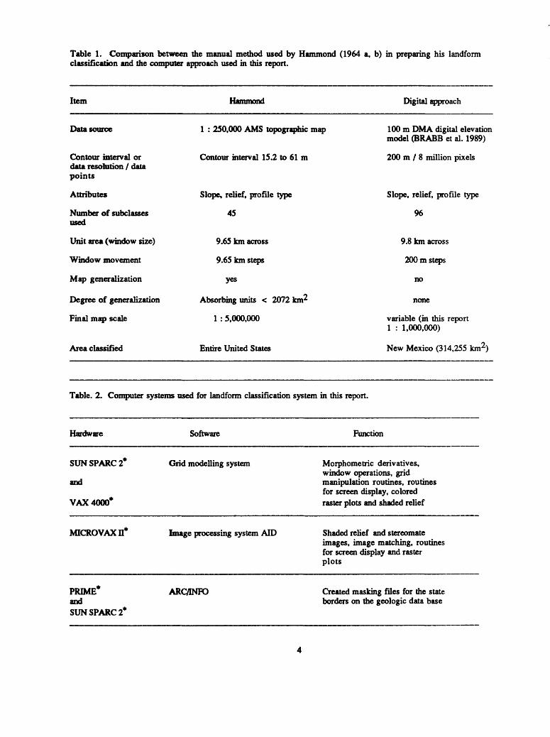
Table 1. Comparison between the manual method used by Hammond (1964 a, b) in preparing his landform classification and the computer approach used in this repon.

Item Hammond Digital approach

Data source

Contour interval or data resolution / data points

Attributes

Number of subclasses

Unit area (window size)

Window movement

Map generalization

Degree of generalization

Final map scale

Area classified

1 : 250,000 AMS topographic map

Contour interval 15.2 to 61 m

Slope, relief, profile type

45

9.65 km across

9.65 km steps

yes

Absorbing units < 2072 km2

1 :5,000,000

Entire United States

100 m DMA digital elevation model (BRABB et al. 1989)

200 m / 8 million pixels

Slope, relief, profile type

96

9.8 km across

200m steps

no

none

variable (in this report 1 : 1,000.000)

New Mexico (314,255 km2)

Table. 2. Computer systems used for landform classification system in this repon.

Hardware Software Function

SUNSPARC2*

and

VAX 4000*

Grid modelling system Morphometric derivatives, window operations, grid manipulation routines, routines for screen display, colored raster plots and shaded relief

MICROVAXn* Image processing system AID Shaded relief and stereomate images, image matching, routines for screen display and raster plots

PRIMEandSUNSPARC2*

ARC/INFO Created masking files for the state borders on the geologic data base

Hammond. The only elevation information available in digital form for the entire state of New Mexico was prepared at a 3 arc-second resolution by the Defense Mapping Agency (DMA) and is now distributed in 1-degree blocks by the U.S. Geological Survey (1990). Spacing of the elevations in this DEM in north-south and east-west profiles is 3 arc-seconds. According to the U.S. Geological Survey (1990), the production objective for this DEM was to satisfy an absolute horizontal accuracy of 130 m and an absolute vertical accuracy of ±30 m. As pointed out in the same report, the relative horizontal and vertical accuracy "will in many cases conform to the actual hypsographic features with higher integrity than indicated by the absolute accuracy." This accuracy was confirmed by Isaacson and Ripple (1990), who compared 7.5- minute DEM data with the DMA 1-degree DEM data sets, and found good correspondences in areas of mountainous terrain.

The 3 arc-second DMA DEM for New Mexico was regridded to 36 million elevation points spaced equally at a ground distance of 100 m by using the technique described in Brabb and others (1989). In order to manipulate the data on our limited computer resources, this regridded DEM was regridded again to a spacing of 200 m ground distance using the grid modeling system mentioned on Table 2. This program selects each second point of the original DEM.

CALCULATION OF SLOPE

The 200 m DEM was converted to a slope map (not shown) by moving a window of 3 by 3 elevation points across the data set in 200 m intervals (see Table 3). On each placement of the window, the 9 points were used to construct a quadratic surface. The slope of this surface, in percent, was assigned to the point in the center of the window (refer to Mark and others, 1988, for diagrams and additional information).

The percentage of areas where slope is less than 8 percent (gentle slopes in the Hammond classification) were then identified by moving a window with 49 by 49 slope points across the data set in 200 m intervals. The area of this window, 9.8 km (6 mi), is close to the 9.65 km used by Hammond. To fit the Hammond classification, the data obtained by this procedure were then divided into areas of less than 20 percent, 20 to 50 percent, 50 to 80 percent, and more than 80 percent gentle slope.

LOCAL RELIEF

A moving window with 49 by 49 elevation points was then moved across the data set in 200 m increments to determine the difference between maximum and minimum elevation. The data obtained by this procedure were then divided into areas where the local relief corresponds to the 6 ranges used by Hammond.

PROFILE TYPE

The profile type is expressed as an index relating the gently sloping areas to upland or lowland situations. Hammond used the profile type to subdivide Tablelands (TAB) as upland units and Plains with Hills or Mountains (PHM) as lowland units.

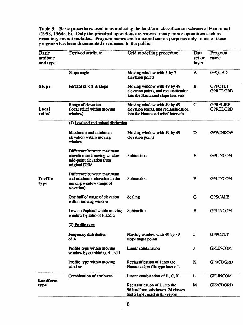
Table 3: Basic procedures used in reproducing the landform classification scheme of Hammond (1958,1964a, b). Only the principal operations are shown-many minor operations such as rescaling, are not included. Program names are for identification purposes only none of these programs has been documented or released to the public.

Basic attribute and type

Slope

Local relief

Profile type

Derived attribute

Slope angle

Percenter <8% slope

Range of elevation (local relief within moving window)

HI f .nwlafld ajltif "pfond distinction

Maximum and minimum elevation within moving window

Difference between maximum elevation and moving window mid-point elevation from original DEM

Difference between maximum and minimum elevation in the moving window (range of

Grid modelling procedure

Moving window with 3 by 3 elevation points

Moving window with 49 by 49 elevation points, and reclassification into the Hammond slope intervals

Moving window with 49 by 49 elevation points, and reclassification into the Hammond relief intervals

Moving window with 49 by 49 elevation points

Subtraction

Subtraction

Data set or layer

A

B

C

D

E

F

Program name

GPQUAD

GPPCTLT GPRCDGRD

GPRELEEF GPRCDGRD

GPWINDOW

GPLINCOM

GPLINCOM

elevation)

Landform type

One half of range of elevation within moving window

Lowland/upland within moving window by ratio of E and G

(2> Profile type

Frequency distribution of A

Profile type within moving window by combining H and I

Profile type within moving window

Combination of attributes

Scaling

Subtraction

Moving window with 49 by 49 slope angle points

Linear combination

Reclassification of J into the Hammond profile type intervals

Linear combination of B, C, K

Reclassification of L into the 96 landform subclasses, 24 classes and 5 tvpes used in this report

G

H

I

J

K

L

M

GPSCALE

GPLINCOM

GPPCTLT

GPLINCOM

GPRCDGRD

GPLINCOM

GPRCDGRD

R "~"~ ~ * * *

1/2R ,

lowland

1/2 R

max elevation within the window

window center

, winrfnw wirith ^

elevation point at window center

min. elevation within the window

max elevation within the window

elevation point at window center

min. elevation within the window

upland:

lowland:

when max. elevationelevation

R

max. elevation - elevation < 1/2 R

max. elevation - elevation > 1/2 R

« maximum elevation within the moving window elevation at moving window center « local relief within the moving window

Figure 2. Schematic diagram of a cuesta scarp slope showing how to determine whether the slope should be classified as an upland or a lowland. A, lowland; B, upland.

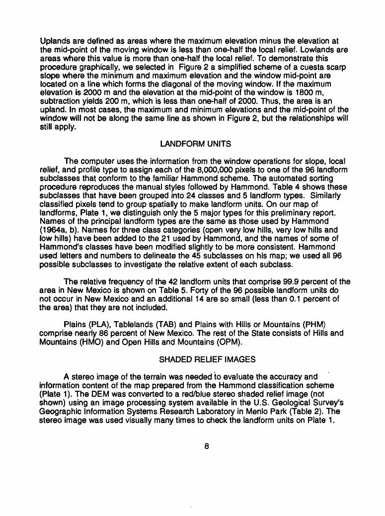
Uplands are defined as areas where the maximum elevation minus the elevation at the mid-point of the moving window is less than one-half the local relief. Lowlands are areas where this value is more than one-half the local relief. To demonstrate this procedure graphically, we selected in Figure 2 a simplified scheme of a cuesta scarp slope where the minimum and maximum elevation and the window mid-point are located on a line which forms the diagonal of the moving window. If the maximum elevation is 2000 m and the elevation at the mid-point of the window is 1800 m, subtraction yields 200 m, which is less than one-half of 2000. Thus, the area is an upland. In most cases, the maximum and minimum elevations and the mid-point of the window will not be along the same line as shown in Figure 2, but the relationships will still apply.

LANDFORM UNITS

The computer uses the information from the window operations for slope, local relief, and profile type to assign each of the 8,000,000 pixels to one of the 96 landform subclasses that conform to the familiar Hammond scheme. The automated sorting procedure reproduces the manual styles followed by Hammond. Table 4 shows these subclasses that have been grouped into 24 classes and 5 landform types. Similarly classified pixels tend to group spatially to make landform units. On our map of landforms, Plate 1, we distinguish only the 5 major types for this preliminary report. Names of the principal landform types are the same as those used by Hammond (1964a, b). Names for three class categories (open very low hills, very low hills and low hills) have been added to the 21 used by Hammond, and the names of some of Hammond's classes have been modified slightly to be more consistent. Hammond used letters and numbers to delineate the 45 subclasses on his map; we used all 96 possible subclasses to investigate the relative extent of each subclass.

The relative frequency of the 42 landform units that comprise 99.9 percent of the area in New Mexico is shown on Table 5. Forty of the 96 possible landform units do not occur in New Mexico and an additional 14 are so small (less than 0.1 percent of the area) that they are not included.

Plains (PLA), Tablelands (TAB) and Plains with Hills or Mountains (PHM) comprise nearly 86 percent of New Mexico. The rest of the State consists of Hills and Mountains (HMO) and Open Hills and Mountains (OPM).

SHADED RELIEF IMAGES

A stereo image of the terrain was needed to evaluate the accuracy and information content of the map prepared from the Hammond classification scheme (Plate 1). The DEM was converted to a red/blue stereo shaded relief image (not shown) using an image processing system available in the U.S. Geological Survey's Geographic Information Systems Research Laboratory in Menlo Park (Table 2). The stereo image was used visually many times to check the landform units on Plate 1.

8

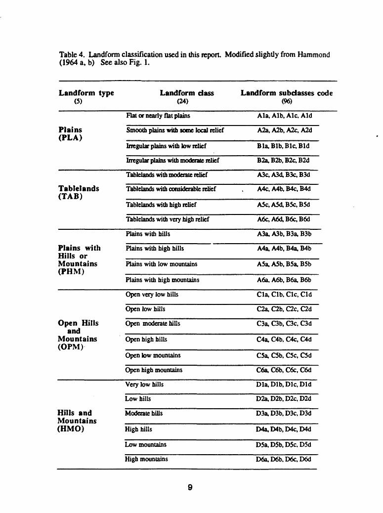
Table 4. Landform classification used in this report Modified slightly from Hammond (1964 a, b) See also Fig. 1.

Landform type(5)

Landform dass(24)

Landform subclasses code(96)

Plains (PLA)

Flat or nearly flat plains

Smooth plains with some local relief

Ala, Alb, Ale, Aid

A2a, A2b, A2c, A2d

Irregular plains with low relief

Irregular plains with moderate relief

Bla.Blb.Blc.Bld

B2a.B2b.B2c.B2d

Tablelands(TAB)

Open Hillsand

Mountains (OPM)

Tablelands with moderate relief

Tablelands with considerable relief

Tablelands with high relief

Tablelands with very high relief

Open very low bills

Open low bills

Open moderate bills

Open high bills

Open low mountains

Open bigb mountains

A3c.A3d.B3c.B3d

A4c.A4b.B4c.B4d

A5c.A5d.B5c.B5d

A6c.A6d.B6c.B6d

Plains with Hills or Mountains (PHM)

Plains with bills

Plains with bigb bills

Plains with low mountains

Plains with bigb mountains

A3a, A3b. B3a, B3b

A4a. A4b. B4a. B4b

A5a.A5b.B5a.B5b

A6a, A6b. B6a, B6b

Cla, Clb, Clc, Cld

C2a, C2b, C2c, C2d

C3a, C3b, C3c, C3d

C4a, C4b, C4c, C4d

C5a, C5b, C5c, C5d

C6a, C6b, C6c, C6d

Hills andMountains(HMO)

Very low hills

Low hills

Moderate bills

High bills

Low mountains

High mountains

Dla,Dlb.Dlc,Dld

D2a.D2b,D2c,D2d

D3a,D3b,D3c,D3d

EMa.D4b.D4c.D4d

D5a,D5b,D5c,D5d

D6a.D6b,D6c.D6d

9

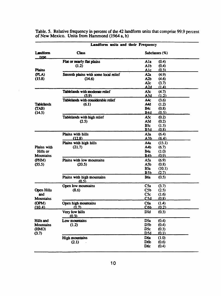
Table. 5. Relative frequency in percent of the 42 landform units that comprise 99.9 percent of New Mexico. Units from Hammond (1964 a, b)

Landform tvpe

Plains<PLA) (15.8)

Tablelands (TAB) (14.5)

Plains with Hills or

Mountains (PHM) (55.5)

Open Hills and

Mountains (OPM) (10.4)

Hills and Mountains (HMO) (3.7)

Landform vnits and their Frequency

Class Subclasses (%)

Flat or nearly flat plains (1.2)

Smooth plains with some local relief (14.6)

Tablelands with moderate relief(5.9)

Tablelands with considerable relief (6.1)

Tablelands with high relief (2.5)

Plains with hills (12.8)

Plains with high hills (21.7)

Plains with low mountains (20.5)

Plains with high mountains (0.5)

Open low mountains (8.6)

Open high mountainsn.T)

Very low hills (0.31

Low mountains (1.2)

High mountains (2.1)

Ala Alb AleA2a A2b A2c A2dA3c A3dA4c A4d B4c B4dA5c A5d B5c B5dA3a A3bA4a A4b B4a B4bA5a A5b B5a B5bB6a

C5a C5b C5c C5dC6a C6bDid

D5a D5b D5c D5dD6a D6b D6c

(0.4) (0.4) (0.3)(4.9) (4.6) (3.7)n.4)(4.7) (1.2)(3.6) (1.2) (0.8) (05)(0.2) (0.2) (1.3) (0.8)(6.4) (6.4)(13.1) (6.7) (1.0) (0.9)(6.9) (0.8) (10.1) (2.7)(0.5)

(3.7) (2.5) (1.6) (0.8)(1.4) (0.2)(0.3)

(0.4) (0.4) (0.3) (01)0.0) (0.6) (0.4)

10

The shaded relief map in this report (Plate 2) was prepared from the 200 m DEM using the method described by Mark and Aitken (1990). A sun azimuth of 315°, located 30° above the horizon, and a vertical exaggeration of 2X were used to prepare the image.

REGIONAL INTERPRETATION

The digital landform map (Plate 1) indicates:

(1) Hills and Mountains (HMO) areas (< 20% gently sloping land) form the core areas, as the term is used by Wood and Snell (1960), of the 9 principal mountain chains: Sangre de Christo, San Juan, San Pedro and San Jemez, Chuska, San Mateo (Mt. Taylor), Monzano and Sandia, Mogollon (including the Black Range, San Mateo and Magdalena Mountains), San Andres, and Sacramento Mountains.

(2) The core areas of these mountain chains (HMO) are surrounded by Open Hills and Mountains (OPM) which may vary significantly in size and shape. For example, the west-facing slopes of the Sacramento Mountains (near Carrizozo) are characterized by OPM units with a 2 to 5 km width, whereas the east-facing slopes have a very broad OPM transition as wide as 10 to 50 km extending to the TAB and PHM of the western Pecos Valley region.

(3) The principal Plain (PLA) regions are located at the southeast and south- central parts of the map, including the upper Pecos River drainage basin and the central parts of the Tularosa Valley (White Sands).

(4) Medium-relief landform units between Hill and Mountains (HMO) and Plain regions (PLA) cover about 70% of the whole state and include Tablelands (TAB; 14.5%) and Plains with Hills and Mountains (PHM; 55.5%). They are created by combining areas with > 50% gently sloping land and local relief values more than 91.5 m (see Figure 1). Because PHM regions are so widespread, some of their characteristics will be discussed in more detail.

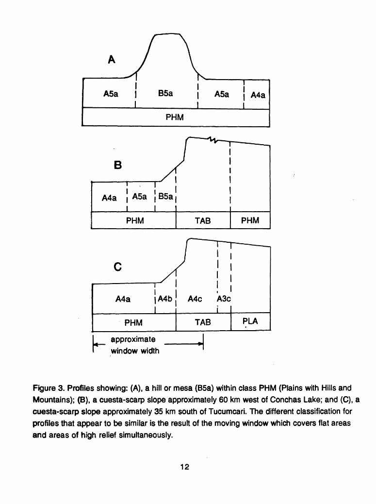
Units A4a, A5a and B5a comprise the largest areal extent (30%) of PHM subclasses. They are located in areas with high percentages of gently sloping land in close proximity to areas with high local relief. Other locations are single hills and mountains on flat plains (Figure 3a). A more detailed comparison with topographic maps at 1:100,000 scale reveals that the transition zones cover gently sloping areas mainly in front of steeply sloping parts of hills, mountains and tablelands. In those areas, they characterize the neighborhood of landforms with higher relief, and they could be used to delimit those units. The transition zones are created by the effects of the moving window, which covers flat areas and areas of higher relief simultaneously (see Figure 3b).

Hammond did not include A-4, A-5, and A-6 units in his classification system (Figure 1). We speculate that he probably absorbed these zones into adjacent classes because they are all smaller than 7 km in maximum width. We put these units provisionally into the corresponding subclasses of TAB and PHM (Table 1).

11

1A5a |

1

1 >

B5a |1

PHM

i A5a | A4a

I

B

A4a | A5a j B5a i IPHM TAB PHM

- . ,

A4a )A4b1

PHM

!A4c A3c

i

TAB

approximate Iwindow width '

PLA

Figure 3. Profiles showing: (A), a hill or mesa (B5a) within class PHM (Plains with Hills and Mountains); (B), a cuesta-scarp slope approximately 60 km west of Conchas Lake; and (C), a cuesta-scarp slope approximately 35 km south of Tucumcari. The different classification for profiles that appear to be similar is the result of the moving window which covers flat areas and areas of high relief simultaneously.

12

(5) Unit TAB occurs exclusively in upland areas, mostly in northeast New Mexico. This part of the State is characterized by extensive cuesta-scarp (mesa) landforms, such as those east of Las Vegas, south of Santa Rosa and south of Tucumcari.

(6) A 50-km-long mesa area approximately 40 km northwest of Conchas Lake has been classified as Open Hills and Mountains (OPM). This different unit within a typical PHM and TAB landscape is explicable by incision of the mesa border and a lower percentage of gentle slope area.

TAB is replaced by PHM (Figure 3b) 20 to 40 km behind the mesa border as the relief diminishes, reflecting the change from upland into lowland classes. A similar change occurs 35 km south of Tucumcari where a tableland strip 5 km wide (including the upper cuesta-scarp slopes) changes into the large plain areas of southeast New Mexico (see Figure 3c).

COMPARISON OF OUR MAPS WITH THOSE OF HAMMOND

As expected, there are differences between the map in this report and the one made by Hammond. These differences are probably caused mainly by different data resolutions and different increments of the moving window. On the other hand, Hammond's landform map is highly generalized and created for scales between 1:3,000,000 and 1:7,000,000. Because no manual or digital generalization procedures were used in this report, a comparison of both maps can only be based on interpreting the main, broad-scaled morphometric structures.

(1) The Plains (PLA) units of our map show a good correspondence with Hammond's classes in the east-southeast part of the state. Both maps classify these regions with A2 attribute combinations. A larger difference is in the flat areas of the Tularosa Valley (appr. 4,000 km2) which is, according to Fenneman (1931), part of the southwest Basin and Range province. In that area, A1 and A2 units are shown on our map where Hammond mapped B6a (PHM) landforms.

(2) In Hammond's map, Tablelands (TAB) cover large regions of the northeast and northwest of New Mexico. This unit is reproduced adequately in the northeast but not in the northwest of the State. In the northwest part, classified by Fenneman (1931) as part of the Colorado Plateau, the digital approach created large areas of PHM units and only small TAB areas.

(3) Plains with Hills or Mountains (PHM) were modelled adequately. These landforms cover the southwest and south-central parts of New Mexico where they are the dominant unit with moderate relief.

(4) Similarly, the Open Hills and Mountains (OHM) of the digital map show very good correspondence with the equivalent units of Hammond's map. These areas are located in the southwest and north of the state. Significant differences are present in the southern San Luis Valley (C5a) between the Sangre de Christo Mountains and the

13

San Juan Mountains and in the foothill regions of the east Sacramento Mountains (C5c) where the digital map shows PHM and TAB units.

(5) Most of the Hills and Mountains (HMO) were reproduced adequately, but on the digital map the areas covered by these units are smaller. In general, Hammond's map shows HMO units in regions where the digital approach created both HMO and OPM areas.

CONCLUSIONS

A computer-derived classification of landforms in an entire state following the manual methodology of Hammond has been prepared. To our knowledge, this is the only successful automation of the Hammond approach yet attempted. The digital method seems to work quite well, providing similar patterns for most of the major landform types and much greater detail for classes and subclasses of landforms. The availability of the DMA DEM for the United States indicates that the entire country could be reclassified in greater detail. Indeed, the landforms in any country or area with a DEM could be classified easily and readily.

ACKNOWLEDGMENTS

We are grateful to Richard Pike for discussions about the Hammond classification and method. Todd Fitzgibbon, Pat Murphy, Ming Ko, and Sam Arriola kindly contributed information about computer programs and methodology. Donna Knifong provided command language to transfer the border of New Mexico from a file of the geology to the map file for this report. Jere Swanson graciously provided image processing procedures for the stereo shaded relief images. Chip Stevens prepared film plots of both the shaded relief and landform classification map. We are also grateful to personnel in the GIS Research Lab, Western Region, for their instruction and support.

REFERENCES

Brabb, E.E., Pampeyan, E.H., and Bonilla, M.G., 1978, Landslide susceptibility in San Mateo County, California: U.S. Geological Survey Miscellaneous Field Studies Map MF-360, scale 1:62,500.

Brabb, E.E., Guzzetti, F., Mark, R., and Simpson, R.W., 1989, The extent of landsliding in northern New Mexico and similar semi-arid regions, in Sadler, P.M and Morton, D.M., eds., Landslides in a semi-arid environment with emphasis on the inland valleys of southern California: Publications of the Inland Geological Society, v. 2, p 163-173.

Cardinal!, M., Guzzetti, F., and Brabb, E., 1990, Preliminary maps showing landslide deposits and related features in New Mexico: U. S. Geological Survey in cooperation with the Research Institute for Hydrogeological Protection in Central Italy, New Mexico Bureau of Mines and Mineral Resources, New Mexico Highway Dept; U.S. Geological Survey Open File Report 90-293, 4 sheets, map scale 1:500,000.

14

Dikau, R., 1989, The application of a digital relief model to landform analysis ingeomorphology, in Paper, J., ed., Three dimensional applications inGeographical Information Systems, London, Taylor& Francis, p. 51-77.

Evans, I.S., with the assistance of Margaret Young and J.S. Gill, 1979, An integratedsystem of terrain analysis and slope mapping: Department of Geography,University of Durham, England, Final Report (Report 6) on U.S. Army ContractDA-ERO-591-73-G0040, Statistical characterization of altitude matrices bycomputer, 192 p.

Fenneman, N.M. 1931, Physiography of the western United States: McGraw-Hill, NewYork, 534 p.

Fenneman, N.M., and Johnson, D.W., 1946. Physical divisions of the United StatesU.S. Geological Survey, 1:7,000,000.

Guzzetti, Fausto, and Brabb, E.E., 1987, Map showing landslide deposits insouthwestern New Mexico: U.S. Geological Survey Open File Report 87-70,scale 1:500,000.

Hammond, E.H. 1954, Small-scale continental landform maps: Annals of Assoc. ofAmerican Geographers v. 44, p. 33-42.

___, 1958, Procedures in the descriptive analysis of terrain; Final Report on ProjectR-387-015: Dept. of Geography, University of Wisconsin, Madison, Wl.

___, 1964a, Analysis of properties in land form geography: An application to broad- scale land form mapping; Annals of Assoc. of American Geographers v. 54, p.11-19.

___, 1964b, Classes of land surface form in the forty-eight states, U.S.A.: AnnualAssoc. American Geographers v. 54; Map supplement no. 4, scale 1:5,000,000.

Isaacson, D.L, and Ripple, W.J., 1990, Comparison of 7.5-minute and 1-degree digitalelevation models: Photogrammetric Engineering & Remote Sensing, v. 56, no.11, p. 1523-1527.

Mark, R.K., Newman, E., and Brabb, E.E., 1988, Slope map of San Mateo County: U.S.Geologial Survey Miscellaneous Investigations Map 1-1257-J, scale 1:62,500.

Mark, R.K., and Aitken, D.S., 1990, Shaded-relief topographic map of San MateoCounty, California: U.S. Geological Survey Miscellaneous Investigations Map I-1257-K, scale 1:62,500.

Mark, R.K., in press, Map of debris-flow probability, San Mateo County, California: U.S.Geological Survey Miscellaneous Investigations Map 1-1257-M, scale 1:62,500.

Newman, E.B., Paradis, A.R., and Brabb, E.E., 1978, Feasibility and cost of using acomputer to prepare landslide susceptibility maps of the San Francisco Bayregion, California: U.S. Geological Survey Bulletin 1443, 27 p.

U.S. Geological Survey, 1980, Classes of land-surface form, in National Atlas, sheetno. 62, adapted from Hammond, E.H., 1964b: U.S. Geological Survey, Reston,VA, scale 1:7,500,000.

___, 1990, Digital elevation models, data users guide 5: U.S. Geological Survey,Reston, VA, 51 p.

Wood, W.F., and Snell, J.B., 1960, A Quantitative System for Classifying Landforms:Natick, Massachusetts, U.S. Army Quatermaster Research and EngineeringCenter, Environmental Protection Research Division, Environmental AnalysisBranch, Technical Report EP-124, 20 p.

15