u.s. department of the interior u.s. geological … · u.s. department of the interior u.s....

U.S. DEPARTMENT OF THE INTERIOR

U.S. GEOLOGICAL SURVEY

MODFLOW-2000 Ground-Water Model—User Guide to the Subsidence and Aquifer-SystemCompaction (SUB) Package

Open-File Report 03— 233

U.S. GEOLOGICAL SURVEY

GROUND-WATER RESOURCES PROGRAM

20

0

30

Uplift

Subsidence

Change inland-surfacealtitude, inmillimeters

U.S. DEPARTMENT OF THE INTERIORU.S. GEOLOGICAL SURVEY

MODFLOW-2000 Ground-Water Model—User Guide to the Subsidence and Aquifer-System Compaction (SUB) Package

By Jörn Hoffmann, S.A. Leake, D.L. Galloway, and Alica M. Wilson

Open-File Report 03—233

U.S. GEOLOGICAL SURVEY GROUND-WATER RESOURCES PROGRAM

Tucson, Arizona2003

U.S. DEPARTMENT OF THE INTERIORGALE A. NORTON, Secretary

U.S. GEOLOGICAL SURVEYCharles G. Groat, Director

The use of firm, trade, and brand names in this report is for identification purposes only and does not constitute endorsement by the U.S. Geological Survey.

For additional information write to:

District Chief U.S. Geological Survey Water Resources Division 520 N. Park Avenue, Suite 221 Tucson, AZ 85719–5035

Copies of this report can be purchased from:

U.S. Geological Survey Information Services Box 25286 Federal Center Denver, CO 80225–0046

Information about U.S. Geological Survey programs in Arizona is available online at http://az.water.usgs.gov.

http://az.water.usgs.gov

Contents iii

CONTENTS

Abstract ................................................................................................................................................................ 1Introduction .......................................................................................................................................................... 2

Purpose and Scope ...................................................................................................................................... 3Previous Studies .......................................................................................................................................... 3Interbeds...................................................................................................................................................... 4

Theory .................................................................................................................................................................. 4Effective Stress and Stress Changes ........................................................................................................... 5Compaction of Compressible Sediments .................................................................................................... 6Time Delays ................................................................................................................................................ 9

Incorporating Interbed Storage into the Ground-Water Flow Equation .............................................................. 11No-Delay Interbeds ..................................................................................................................................... 11Delay Interbeds ........................................................................................................................................... 13

Package Output .................................................................................................................................................... 17Input Instructions.................................................................................................................................................. 21

Explanation of Fields Used in Input Instructions........................................................................................ 22Practical Considerations for the Use of the SUB Package................................................................................... 27

Compatibility of the SUB Package with Versions of MODFLOW............................................................ 27Simulation of Flow in and Compaction of Confining Units ....................................................................... 27Use of Steady-State Stress Periods in MODFLOW-2000 .......................................................................... 28Improvement of Convergence in Solutions of Coupled Equations............................................................. 29

Sample Simulations.............................................................................................................................................. 29Sample Problem 1 ....................................................................................................................................... 29Sample Problem 2 ....................................................................................................................................... 31Sample Problem 3 ....................................................................................................................................... 33

Applicability, Assumptions, and Limitations....................................................................................................... 36References Cited .................................................................................................................................................. 37Appendix .............................................................................................................................................................. 43

Contents iv

FIGURES

1. Diagram showing poorly permeable interbeds within a relatively permeable confined aquifer, bounded at top and bottom by confining units. .................................................................................... 5

2. Graph showing theoretical relation between effective stress and layer thickness for a hypothetical compressible bed .................................................................................................................................. 8

3. Diagram showing finite difference cells and nodes used in numerical approximation given by equation 11 ............................................................................................................................ 10

4. Example of volumetric budget for systems of delay interbeds. ........................................................... 195. Diagrams showing compressible beds in an aquifer system and two approaches to

representing the confining unit in the MODFLOW simulation of aquifer-system compaction using the SUB PackageA. Vertical section of an aquifer system with compressible sediments within and

adjacent to aquifers ....................................................................................................................... 28B. Use of one model layer to simulate flow and storage changes in the confining unit ................... 28C. Use of five model layers to simulate flow and storage changes in the confining unit.................. 28

6. Graphs showing sample problem 1: Model configuration and comparisons of simulated compaction with analytical solution for compactionA. Model setup of interbed drainage as a result of step decrease in head in the aquifer................... 30B. Comparison of the compaction history simulated by the Subsidence and Aquifer-System

Compaction Package with the analytical solution to the problem................................................ 30 C. Difference between analytical solution and simulated compaction ............................................. 30

7. Diagnosis showing sample problem 2: Model configuration used to simulate seasonally fluctuating stresses................................................................................................................................ 31

8–10. Graphs showing: 8. Sample problem 2: Head and compaction time series for no-delay and delay interbeds..................... 329. Sample problem 3: Hypothetical ground-water basin.

A. A plan view of a ground-water basin showing contours of head prior to pumping in the uppermost layer ...................................................................................................................... 33

B. Vertical cross section showing aquifers, confining unit, and model layer designations............... 3310. Sample problem 3: Simulated hydraulic head and compaction and land subsidence time series ........ 35

TABLES

1. Information optionally printed or saved by the Subsidence and Aquifer-System Compaction Package and associated variable names, numbers of arrays, and array names .................................... 18

2. Hydrologic properties of the fine-grained sediments used in sample problem 3 ................................. 343. Thickness of individual interbeds thicker than 1.5 m in layers 1 and 3 of sample problem 3 ............. 344. Computation of the elastic and inelastic storage coefficients for sample problem 3 ........................... 35

CONVERSION FACTORS

Multiply By To obtain

millimeter (mm) 0.03937 inch

centimeter (cm) 0.3937 inch

meter (m) 3.281 foot

kilometer (km) 0.6214 mile

cubic meter per day (m3/d) 35.31 cubic foot per day

liter per second (L/s) 15.85 gallon per minute

cubic meter per day (m3/d) 264.2 gallon per day

meter per day (m/d) 3.281 foot per day

per meter (m-1) 0.3048 per foot

ACRONYMS

BCF Block-Centered Flow

IBS1, 2 Interbed Storage Package, version 1, 2

HUF Hydrogeologic Unit Flow

LPF Layer-Property Flow

PCG Preconditioned Conjugate Gradient

SIP Strongly Implicit Procedure

SUB Package Subsidence and Aquifer-System Compaction Package

USGS U.S. Geological Survey

Contents v

Contents vi

MODFLOW-2000 Ground-Water Model—User Guide to the Subsidence and Aquifer-System Compaction (SUB) Package

By Jörn Hoffmann, S.A. Leake, D.L. Galloway, and Alicia M. Wilson

Abstract

This report documents a computer program, the Subsidence and Aquifer-System Compaction (SUB) Package, to simulate aquifer-system compaction and land subsidence using the U.S. Geological Survey modular finite-difference ground-water flow model, MODFLOW-2000. The SUB Package simulates elastic (recoverable) compaction and expansion, and inelastic (permanent) compaction of compressible fine-grained beds (interbeds) within the aquifers. The deformation of the interbeds is caused by head or pore-pressure changes, and thus by changes in effective stress, within the interbeds. If the stress is less than the preconsolidation stress of the sediments, the deformation is elastic; if the stress is greater than the preconsolidation stress, the deformation is inelastic. The propagation of head changes within the interbeds is defined by a transient, one-dimensional (vertical) diffusion equation. This equation accounts for delayed release of water from storage or uptake of water into storage in the interbeds. Properties that control the timing of the storage changes are vertical hydraulic diffusivity and interbed thickness. The SUB Package supersedes the Interbed Storage Package (IBS1) for MODFLOW, which assumes that water is released from or taken into storage with changes in head in the aquifer within a single model time step and, therefore, can be reasonably used to simulate only thin interbeds. The SUB Package relaxes this assumption and can be used to simulate time-dependent drainage and compaction of thick interbeds and confining units. The time-dependent drainage can be turned off, in which case the SUB Package gives results identical to those from IBS1.

Three sample problems illustrate the usefulness of the SUB Package. One sample problem verifies that the package works correctly. This sample problem simulates the drainage of a thick interbed in response to a step change in head in the adjacent aquifer and closely matches the analytical solution. A second sample problem illustrates the effects of seasonally varying discharge and recharge to an aquifer system with a thick interbed. A third sample problem simulates a multilayered regional ground-water basin. Model input files for the third sample problem are included in the appendix.

Abstract 1

INTRODUCTION

Land subsidence is a sudden sinking or gradual settling of the Earth’s surface owing to movement of earth

materials. In the United States, more than 44,000 km2 in 45 states, an area roughly the size of New Hampshire and Vermont combined, has been directly affected by subsidence caused by aquifer-system compaction, drainage of organic soils, underground mining, hydrocompaction of near-surface deposits, natural compaction, sinkholes, petroleum reservoir compaction, tectonism, thawing permafrost, and other processes (National Research Council, 1991). More than 80 percent of the identified subsidence in the Nation is a consequence of human impact on subsurface water, and the increasing development of land and water resources probably will exacerbate existing land-subsidence problems and initiate new ones. Though no strict accounting has been made, it is likely that most of this water-related sub-sidence is caused by the compaction of compressible sediments in and around areas of extensive ground-water pumping. Land subsidence attributable to the compaction of aquifer systems is an often overlooked hazard and an environmental consequence of ground-water withdrawal (Galloway and others, 1999) in many areas. The arid Southwestern United States is especially vulnerable because surface-water supplies are limited and ground water in unconsolidated basin-fill deposits is extensively relied upon. Coastal regions also are commonly affected because they are often underlain by unconsolidated, compressible coastal-plain and shallow-marine sediments. Some of the hazards and environmental consequences include damage to engineered structures (such as buildings, roadways, pipelines, aqueducts, sewerages, and well casings), earth fissures, enhanced coastal and riverine flooding, loss of saltwater- and freshwater-marsh ecosystems, and reactivation of surface faults creating new potential pathways for surface runoff to contaminate aquifers.

For purposes of this report, compaction refers to the change in vertical thickness that accompanies changing stresses on the aquifer system. A decrease in thickness of an interbed is referred to as a positive value of compaction, and an increase as a negative value. All aquifer systems undergo some degree of deformation in response to changes in stress. The seasonal cycle of recharge and discharge from unconsolidated heterogeneous aquifer systems typically causes measurable elastic (recoverable) compaction (Riley, 1969; Poland and Ireland, 1988; Heywood, 1997) and commensurate uplift and subsidence (millimeters to centimeters) of the land surface (Amelung and others, 1999; Bawden and others, 2001; Hoffmann and others, 2001; Lu and Danskin, 2001). Removing water from storage in the fine-grained silts and clays interbedded in the aquifer system causes these highly compressible sediments to compact, resulting in land subsidence. Fine-grained interbeds and confining units within or adjacent to unconsolidated aquifers that undergo head changes related to the development of the ground-water resource are particularly susceptible to compaction. As ground water is drained to the coarser-grained sediments that constitute the aquifers, compaction can occur elastically (recoverable) or inelastically (non-recoverable) causing permanent subsidence, depending on the stress history of these interbeds and confining units.

When an unconsolidated heterogeneous aquifer system is developed as a ground-water resource, most of the ground water produced comes initially from storage in the aquifers, the more permeable interbeds, and the fringes of thicker interbeds and confining units. After some time, when lowered heads in the adjacent aquifers have established vertical head gradients between the aquifers and the interior parts of the thicker or less permeable interbeds and confining units, ground water flows from the interbeds and confining units to the aquifers. When the magnitude and areal extent of the head decline in the aquifers become large, a significant fraction of the water supplied to pumping wells can be derived from ground water released from storage in the interbeds and confining units (Poland and others, 1975).

In confined aquifer systems, the water supplied to pumping wells is derived from the expansion of the water and the compression of the sediments that constitute the matrix or granular skeleton of the aquifer system (Jacob, 1940). Water compressibility and matrix compressibility, along with porosity, determine the storativity of the aquifers and of the interbeds and confining units in the aquifer system. Typically, skeletal compressibilities (and therefore storativities) of interbeds and confining units are several orders of magnitude larger than compressibilities of coarser-grained aquifers, which are typically much larger than water compressibility, therefore, virtually all of the water derived from interbed and confining-unit storage is due to the compressibility of the granular skeleton.

2 MODFLOW-2000 Ground-Water Model—User Guide to the Subsidence and Aquifer-System Compaction (SUB) Package

The storativities of the interbed and confining units and the drainage of these units largely govern the compaction of these aquifer systems and account for all but a negligible amount of the land subsidence that often accompanies ground-water development in these aquifer systems.

Simulation tools for characterizing, understanding, and predicting responses of aquifer systems to stresses imposed by ground-water development are needed to help improve management of ground-water resources. The process of aquifer-system compaction has not been routinely incorporated in ground-water flow models. Because of the growing need to simulate aquifer-system compaction and land subsidence and to improve the capability to do so, a new simulation package was developed for MODFLOW-2000 (Harbaugh and others, 2000), a computer program that simulates three-dimensional ground-water flow. The package is called the Subsidence and Aquifer-System Compaction Package and is referred to as the SUB Package or simply SUB in this report.

Purpose and Scope

This report documents a method for simulating the drainage, changes in ground-water storage, and compaction of aquifers, interbeds and confining units that constitute an aquifer system. Delays in the release of ground water from interbed storage, and thus delays in aquifer-system compaction, can be simulated. Delayed drainage and compaction in confining units can also be simulated.

The SUB Package, consisting of five subroutines, or modules, has been incorporated into the modular finite-difference ground-water flow model, MODFLOW-2000 (Harbaugh and others, 2000). The basis for the SUB Package was developed for earlier versions of MODFLOW as the Interbed Storage Package, version 2 (IBS2; Leake, 1990). IBS2 has neither been formally documented nor released for use with MODFLOW, but has been used internally by the U.S. Geological Survey (USGS) for research and demonstration purposes. SUB updates and documents the IBS2 Package and is a follow-on to the documented MODFLOW package, IBS1 (Leake and Prudic, 1991), in which the delay in release of ground water from compressible interbeds is ignored. SUB also can be set to ignore this delay for some or all interbeds; it then gives the same results as IBS1 for those interbeds.

In addition to accounting for delayed changes in storage, SUB calculates net compaction and elastic expansion of interbeds and aquifers in individual model layers and sums those values to calculate changes in the vertical position of land surface. This report includes a description of how the package computes inelastic (permanent) compaction of sediments as well as elastic (recoverable) compaction. Also included is a description of how the delayed release of ground water from interbed storage is incorporated in the model. The simulation of flow and compaction of confining units is discussed in a separate section of this report. Three simple sample problems are posed and solved to demonstrate the applicability of the SUB Package. A set of data-input files is provided for the third problem to guide the user in setting up input files. Input instructions, discussions of program output, and practical considerations for use of the SUB Package are presented in separate sections of this report.

Only the vertical component of displacement is simulated using SUB. Though theoretically and practically some horizontal displacement occurs in aquifer systems in response to pumping and seasonal recharge/discharge stresses (Wolff, 1970; Carpenter, 1993; Helm, 1994; Hsieh, 1996; Bawden and others, 2001; Burbey, 2001), these displacements tend to be highly localized and occur near pumping wells, near local heterogeneities, and near the margins of ground-water basins. At regional scales and for regional ground-water flow and aquifer-system compaction models, the local horizontal displacements contribute little to the overall change in ground-water storage, and SUB ignores them.

Previous Studies

Numerical models to simulate and predict aquifer-system compaction were developed during the last three decades of the 1900s with the advent of digital computers capable of solving large systems of finite-difference and finite-element equations. New methods to simulate compaction in aquifer systems were developed by Gambolati

Introduction 3

(1970, 1972a,b), Gambolati and Freeze (1973), Helm (1975, 1976), Narasimhan and Witherspoon (1977), and Neuman and others (1982). The one-dimensional (vertical) model presented by Helm computes compaction caused by specified water-level changes. This approach is used to analyze compaction at borehole extensometer sites for which there are detailed records of compaction and water-level changes (Epstein, 1987; Hanson, 1989). More recent efforts have focused on incorporating subsidence calculations in widely used two- or three-dimensional models of ground-water flow. Meyer and Carr (1979), Williamson and others (1989), and Morgan and Dettinger (1996) modified and used finite-difference models to simulate ground-water flow and subsidence in the area of Houston, Texas; the Central Valley, California; and Las Vegas Valley, Nevada, respectively.

Leake and Prudic (1991) developed the Interbed Storage Package, version 1 (IBS1), to simulate regional-scale compaction of interbeds within aquifers using the ground-water model program, MODFLOW (McDonald and Harbaugh, 1988). IBS1 also can be used to simulate compaction of confining units if these units can be discretized into one or more model layers (Larson and others, 2001; Nishikawa and others, 2001). MODFLOW and the IBS1 Package also have been used to simulate regional ground-water flow and land subsidence (Hanson and others, 1990; Hanson and Benedict, 1994; Nishikawa and others, 2001; Hanson and others, 2002; Kasmarek and Stromm, 2002), and one-dimensional ground-water flow and compaction measured at a borehole extensometer site (Sneed and Galloway, 2000). The IBS1 Package assumes that during one model time step, head changes in aquifer material are propagated throughout the entire thickness of compressible interbeds. Thus, the release of water from or uptake of water into interbed storage during this time step represents the full volume specified by the interbed storage coefficients and the change in aquifer hydraulic head. To eliminate this assumption, Leake (1990) developed the Interbed Storage Package, version 2 (IBS2). SUB allows the user to designate some systems of interbeds for which delay in release of water will be calculated. A similar approach was taken by Shearer and Kitching (1994) to simulate ground-water flow and subsidence, accounting for the time-dependent drainage and compaction of thick clay units. Leake (1990) presented the general theory of the IBS2 Package. Although the computer program was not documented for release, previous studies used this approach to investigate the potential effects of land subsidence in the presence of delay interbeds (for example, Leake, 1990, 1991; and Wilson and Gorelick, 1996). This report updates and documents the IBS2 Package as the SUB Package in a form that is compatible with MODFLOW-2000 (Harbaugh and others, 2000). SUB retains the full functionality of the IBS1 Package.

Interbeds

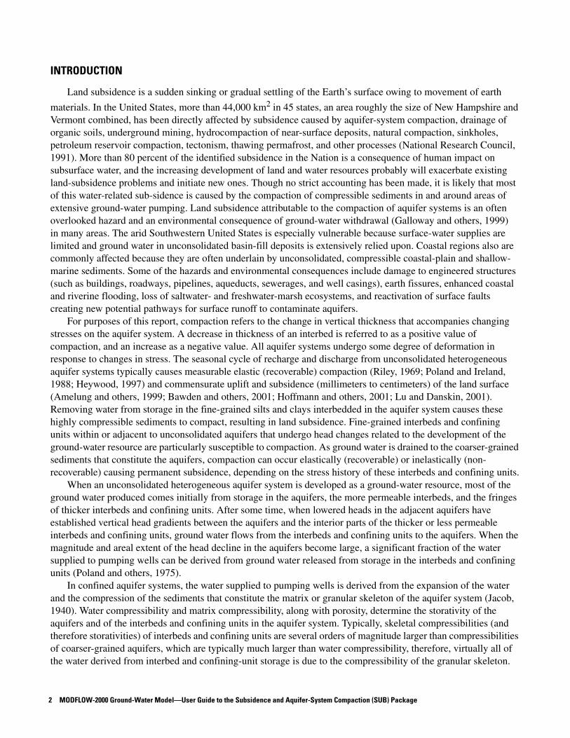
The term interbed is used in this report to denote a poorly permeable bed within a relatively permeable aquifer (fig. 1). Such interbeds are assumed to (1) consist of highly compressible clay and silt deposits from which water flows vertically to adjacent coarse-grained beds, (2) be of insufficient lateral extent to be a confining unit that separates adjacent aquifers, (3) have relatively small thickness in comparison to lateral extent, and (4) have a significantly lower hydraulic conductivity than the surrounding sediments (considered to be aquifer material), yet be porous and permeable enough to uptake or release water in response to head changes in the adjacent aquifer material.

THEORY

In this section, the theoretical basis for the computation of interbed compaction is presented. The development is based on the Terzaghi (1925) theory of one-dimensional consolidation that ignores horizontal strains and stress gradients. The limitations resulting from these assumptions are discussed below.

The details of the numerical implementation of the principles are discussed in the following section. The assumptions and simplifications on which the mathematical representation in the SUB Package for MODFLOW-2000 relies also are presented.


Confining unit

Confining unit

Aquifer

Interbeds

Figure 1. Poorly permeable interbeds within a relatively permeable confined aquifer, bounded at top and bottom by confining units.

Effective Stress and Stress Changes

The coupling of sediment compaction and changes in hydraulic head is based on the Terzaghi (1925) principle of effective stress,

σ′ij σij δijp–= , (1)

where

σ′ij is a component of the effective stress tensor,

σij is a component of the total stress tensor,

δij is the Kronecker delta function, and

p is the fluid pore pressure.

Equation 1 shows that changes in the effective stress can result from changes in the total stress or changes in pore pressure. The total stress is given by the geostatic load of the overlying saturated and unsaturated sediments and tectonic stresses. If the interbeds are assumed to be horizontal and laterally extensive with respect to their thickness, the changes in pore-pressure gradients within the interbeds will be primarily vertical. Assuming that the resulting strains also are primarily vertical (zz), a one-dimensional form of equation 1 can be expressed as

σ′zz σzz p–= . (2)

For purposes of this report it is assumed that the total stress remains constant in time, that is, ∆σzz = 0. Thus, the method presented applies only to sediment compaction in confined aquifers subject to a constant geostatic load.

Analyses of saturated ground-water flow systems commonly use hydraulic head rather than pore pressure. Total hydraulic head is the sum of the pressure head and the elevation head,

h pρwg---------- he+= , (3)

Theory 5

where

h is total hydraulic head,

ρw is the density of water,

g is the gravitational acceleration, and

he is the elevation head referenced to an arbitrary datum.

A change in effective stress resulting from a given head change generally differs in confined and unconfined (water-table) aquifers. In an unconfined aquifer, a change in head corresponds to a draining or re-wetting of pore space and results in a change in the geostatic load or the total stress on the underlying sediments as well as the pore pressure. The change in effective stress caused by a head change in the saturated portion of an unconfined aquifer can be described as (Poland and Davis, 1969, p. 195)

∆σ′zz ρwg 1 n nw+–( )∆h–= , (4)

where

∆σ′zz is the change in vertical effective stress (positive for increase),

n is the aquifer porosity,

nw is the moisture content in the unsaturated zone, as a fraction of total volume, and

∆h is the change in head.

Note that changes in head in an unconfined aquifer, which represent changes in the position of the water table, constitute a mass change in that aquifer. This represents a change in the total stress for all underlying confined aquifers.

In a confined aquifer, the total stress changes negligibly with changes in pore pressure as water is released from or is taken into storage by the saturated porous medium as a result of the compression or expansion of the medium and (or) the water. The change in water density associated with the expansion or compression of the water is negligible. Thus the change in effective stress for a given change in head can be expressed as (Poland and Davis, 1969, p. 195)

∆σ′zz ρwg∆h–= . (5)

The SUB Package was designed to simulate compaction and storage changes in confined aquifer systems and is thus based on equation 5. For interbeds in the saturated part of an unconfined aquifer where hydraulic-head variations are occurring, this approach will overestimate the change in effective stress, thereby overestimating sediment compaction by the factor (1 – n + nw)–1 (see equation 4).

Compaction of Compressible Sediments

Changes in effective stress cause compaction and expansion of the sediments constituting many aquifer systems. In this report, the term compaction is used to describe a reduction in the thickness of a horizontal interbed. A negative compaction signifies an expansion or increased thickness of the interbed. The compressibility, α, of the sediments is defined as

α

dVV

-------–

dσ'----------= , (6)


where

dV is the change in volume of a control volume with initial volume V, and

dσ′ is the change in effective stress.

Absent horizontal displacements, a one-dimensional compressibility can be defined as

α

dbb

------–

dσ'zz------------= , (7)

where

db is the change in thickness of a control volume with initial thickness b.

If the change in effective stress is due only to a change in the pore pressure, equation 5 can be used to express equation 7 as

ρwgαb Sskb= Skdbdh------= = , (8)

where

Ssk is ρwgα , the skeletal specific storage,

Sk is Sskb , the skeletal storage coefficient, and

dh is the change in hydraulic head.

Laboratory consolidation tests on sediment cores and measurements of aquifer-system compaction obtained from borehole extensometers indicate that the compressibility, and thus the skeletal specific storage, can assume very different values depending on whether the effective stress exceeds the previous maximum effective stress, termed the preconsolidation stress (Johnson and others, 1968; Riley, 1969; Jorgensen, 1980).

If the effective stress remains less than the preconsolidation stress, a further increase in effective stress (or decrease in hydraulic head) causes a small elastic compaction in both coarse- and fine-grained sediments. This compaction is recoverable if the effective stress returns to its initial value. In the elastic range, the compressibility, and thus ultimate compaction, is generally slightly greater for fine-grained sediments than for coarse-grained sediments. If the effective stress exceeds the preconsolidation stress, many fine-grained sediments compact inelastically. Inelastic compaction is explained by a physical rearrangement of the grains in the sediments (Meade, 1964) and is largely permanent. Inelastic compaction of coarse-grained sediments is generally negligible compared to that of fine-grained sediments. For the same magnitude of changes in effective stress, inelastic compaction of fine-grained sediments can be one to two orders of magnitude larger than elastic compaction (Riley, 1969, 1998).

Even if the effective stress remains consistently above or below the preconsolidation stress, the compressibility and skeletal specific storage are a function of the effective stress (fig. 2). For some sediments inelastic compaction is approximately proportional to the logarithm of the effective stress (Jorgensen, 1980). However, in many cases applicable to aquifer-system compaction where incremental changes in effective stress are typically small, the relation (eq. 8) can be linearized as

∆b Sk∆h= , (9)

Theory 7

where

∆b is the change in thickness of the sediment layer,

Sk is the skeletal storage coefficient, and

∆h is the change in hydraulic head.

To account for the marked change of the skeletal specific storage when the effective stress exceeds the preconsolidation stress, two separate values are often used (fig. 2):

Ssk

Sske for σ'zz σ'zz max( )<

Sskv for σ'zz σ'zz max( )≥⎩⎨⎧

= , (10)

where

Sske is the elastic skeletal specific storage,

Sskv is the inelastic, or virgin, skeletal specific storage, and

σ'zz(max) is the preconsolidation stress.

LAY

ER

TH

ICK

NE

SS

, IN

ME

TE

RS

11

10

9

8

7

63 4 5 6

∆h = 100 meters

7 8 9 10 11 12 132

EFFECTIVE STRESS, IN 106 PASCALS

Elasticdeformation

Inelastic

compaction


Figure 2. Theoretical relation between effective stress and layer thickness for a hypothetical compressible bed. The gray area indicates the change in effective stress caused by a 100-meter change in hydraulic head. For most hydrologic applications, the relation between change in stress and change in thickness can be linearized. The skeletal storage coefficient is related to the slope of the curve, db/dσ'.

For many fine-grained sediments, Sskv is much greater than Sske. Using two constant values for the skeletal specific storage, one each for stresses greater than and less than the preconsolidation stress, linearizes the nonlinear stress/compaction relation with respect to the preconsolidation stress. The resulting constitutive law represented by equation 9 therefore only approximates the true stress/compaction relation of the sediments.

Using this linearized form of the constitutive law introduces errors into the calculations (examples are given by Narasimhan and Witherspoon, 1977, and Bethke and Corbett, 1988). Leake and Prudic (1991) estimated this error by comparing compaction computed using the linearized equations with compaction computed using a more complex treatment where Sskv is proportional to log σ′zz. Their results indicated that using the linearized form overestimates compaction by about one-half the percentage increase in effective stress. For example, if the effective stress increases by 10 percent, compaction would be overestimated by about 5 percent. For sediments relatively deep below the land surface, a given decline in head will result in a smaller percentage increase in effective stress than for shallower sediments. For many aquifer systems, increases in effective stress are a relatively small percentage of the initial state of stress. For aquifer systems stressed by ground-water development, small errors in compaction can be minimized by selecting the constant Sskv on the basis of an effective stress in the center of the range of stress change, rather than at the beginning. Alternatively, specific storage values used in the SUB Package can be changed with time, if necessary, by restarting a simulation with new storage values.

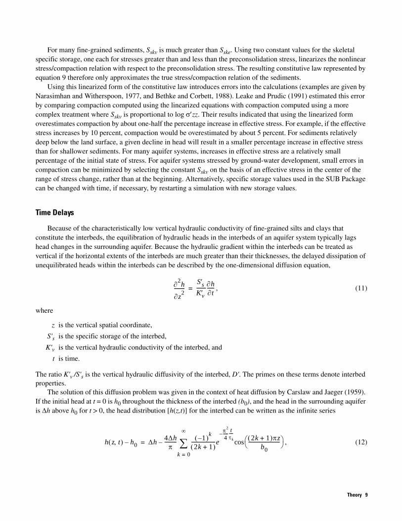
Time Delays

Because of the characteristically low vertical hydraulic conductivity of fine-grained silts and clays that constitute the interbeds, the equilibration of hydraulic heads in the interbeds of an aquifer system typically lags head changes in the surrounding aquifer. Because the hydraulic gradient within the interbeds can be treated as vertical if the horizontal extents of the interbeds are much greater than their thicknesses, the delayed dissipation of unequilibrated heads within the interbeds can be described by the one-dimensional diffusion equation,

∂2h

∂z2---------

S′sK′v--------∂h

∂t------= , (11)

where

z is the vertical spatial coordinate,

S's is the specific storage of the interbed,

K'v is the vertical hydraulic conductivity of the interbed, and

t is time.

The ratio K'v /S's is the vertical hydraulic diffusivity of the interbed, D'. The primes on these terms denote interbed properties.

The solution of this diffusion problem was given in the context of heat diffusion by Carslaw and Jaeger (1959). If the initial head at t = 0 is h0 throughout the thickness of the interbed (b0), and the head in the surrounding aquifer is ∆h above h0 for t > 0, the head distribution [h(z,t)] for the interbed can be written as the infinite series

h z t,( ) h0– ∆h 4∆hπ

---------- 1–( )k

2k 1+( )--------------------e

π2

4-----–

tτk----

2k 1+( )πzb0

--------------------------⎝ ⎠⎛ ⎞cos

k 0=

∞

∑–= , (12)

Theory 9

where the time constant, τk, is defined as

τk

b02-----⎝ ⎠

⎛ ⎞2

S ′s

2k 1+( )2K ′v-------------------------------= . (13)

In equation 12, z = 0 is assumed to be at the midplane of the interbed, with the boundaries at ±b0/2 (fig. 3). Note that both the coefficients in the sum and the τk decrease as k increases. Thus, the true head distribution can be adequately described by a finite number of addends (k), particularly for later times. In the context of interbed compaction and land subsidence, the time delay caused by slow dissipation of transient overpressures is often given in terms of the time constant

τ0

b02-----⎝ ⎠

⎛ ⎞2

S ′s

K ′v---------------------

b02-----⎝ ⎠

⎛ ⎞2

D′--------------== , (14)

which is the time during which about 93 percent of the ultimate compaction for a given decrease in head occurs (Riley, 1969).

Midplane(no flow)

Aquifer

Delay interbed

Aquifer

NN

NN–1z = 0

∆z

z = – b02

z = b02


Figure 3. Finite difference cells and nodes used in numerical approximation given by equation 11. The symmetry of the problem is exploited by computing the heads at nodes for only one-half of the interbed. z is the vertical coordinate referenced to a datum, b is the interbed thickness, NN is the number of finite-difference nodes used to discretize the interbed half-thickness, ∆z is the spacing between finite-difference nodes.

Because τ0 is proportional to S′s, which generally is much larger for inelastically deforming interbeds than for elastically deforming interbeds, deformation in elastically deforming interbeds is often assumed to occur instantaneously. The same is true for very thin inelastically deforming interbeds. Thus, equation 14 can be used to determine in which interbeds the time constant exceeds the model time step, necessitating consideration of incorporating delayed drainage processes.

INCORPORATING INTERBED STORAGE INTO THE GROUND-WATER FLOW EQUATION

Models designed to simulate regional ground-water flow typically solve a form of the equation

∂∂x----- Kxx

∂h∂x------⎝ ⎠

⎛ ⎞ ∂∂y----- Kyy

∂h∂y------⎝ ⎠

⎛ ⎞ ∂∂z----- Kzz

∂h∂z------⎝ ⎠

⎛ ⎞ W–+ + Ss∂h∂t------= , (15)

where

x is the Cartesian coordinate in the x direction,

y is the Cartesian coordinate in the y direction,

z is the Cartesian coordinate in the z direction,

Kxx is the component of the hydraulic conductivity tensor in the x direction,

Kyy is the component of the hydraulic conductivity tensor in the y direction,

Kzz is the component of the hydraulic conductivity tensor in the z direction,

W is the volumetric flux per unit volume of sources and (or) sinks of water, and

Ss is the specific storage.

The term on the right-hand side describes the rate of flow into or out of storage per unit volume of aquifer material. If the aquifer system includes compressible sediments, this term can be multiplied by (1 –γ), where γ is the fraction, by volume, of compressible interbeds in the aquifer system. The storage of the compressible interbeds is represented by a second term added to the right-hand side. Equivalently, the water entering the flow system from interbeds can be added to the source term W. The following sections describe the two ways in which interbed storage is accounted for in the SUB Package.

No-Delay Interbeds

In this report, the term “no-delay interbeds” is used to denote the interbeds for which τ0 is short compared to the time steps used in the simulation. For these interbeds, it is not necessary to explicitly simulate the slow drainage process described in the following section. The treatment in this section therefore ignores the time delays owing to slow dissipation of head transients within the interbeds and assumes that heads everywhere equilibrate instantaneously with the head in the surrounding aquifer. This is the theory previously implemented in the IBS1 Package (Leake and Prudic, 1991). For these interbeds, the flow per unit volume, q̂ , is as follows:

q̂ γS′sk∂h∂t------ with = S′sk

S′ske for h hmin>

S′skv for h hmin≤⎩⎨⎧

= , (16)

Incorporating Interbed Storage into the Ground-Water Flow Equation 11

where

hmin is the lowest previous head or the equivalent preconsolidation stress expressed in terms of preconsolidation head.

The term q̂ can be combined with the source term, W, or added to the right-hand side of equation 15. S'sk is the skeletal specific storage, which assumes an elastic or inelastic (virgin) value depending on whether the head is above or below hmin. Here, hmin is used to define the preconsolidation stress in terms of a preconsolidation head. Note that this is equivalent to equation 10, with the assumption that the total stress (geostatic load) remains constant, and therefore assumes that the water levels in any overlying unconfined aquifers remain approximately constant. Similarly, the compaction of these interbeds can be determined directly from equation 9.

Depending on the flow package used, the MODFLOW-2000 program (Harbaugh and others, 2000) requires the specification of either the dimensionless storage coefficient for each model layer [Block-Centered Flow (BCF) Package (Harbaugh and others, 2000)], or the specific storage for each model layer [Layer-Property Flow (LPF) Package (Harbaugh and others, 2000)], or hydrogeologic unit [Hydrogeologic Unit Flow (HUF) Package (Anderman and Hill, 2000)]. The storage values for no-delay interbeds are specified in the model by their skeletal storage coefficients, S′ke S′skeb0= and S′kv S′skvb0= , rather than by their elastic and inelastic skeletal specific-storage values, S′ske and S′skv, respectively. Many no-delay interbeds in a model layer can be grouped into a system of no-delay interbeds. A system of interbeds is assigned total elastic and total inelastic skeletal storage coefficients in the SUB input file (variables Sfe and Sfv in the input instructions). A representative skeletal storage coefficient for all N no-delay interbeds of a system can be computed by:

S′k S′ki

i 1=

N

∑ S′skibi

i 1=

N

∑= = . (17)

Storage changes and the corresponding compaction in the interbeds are computed at every time step. These computations must account for any elastic storage changes from changes in head in a time step above the level of the preconsolidation head at the end of the previous time step, as well as any inelastic storage changes from decreases in head below the preconsolidation head. The expression that accounts for total flux (flow per unit area), q, into or out of elastic and (or) inelastic skeletal storage at cell i for time-step m is

qim S′k

m

∆tm----------- hm H m 1–

–( )S′ke

∆tm--------- H m 1– hm 1–

–( )+= , (18)

where

S′km S′ke for hm H m 1–>

S′kv for hm H m 1–≤⎩⎪⎨⎪⎧

= ,

where the superscripts denote the time step. The quantities hm and Hm-1 are the head at the end of time-step m and the preconsolidation head at the end of time-step m–1, respectively, and ∆tm is the length of the mth time step. The compaction at cell i during time-step m is computed by multiplying qi

m by the length of the time step ∆tm. Using this approach permits the use of larger time steps without incurring significant errors caused by the typically large difference between the inelastic and elastic skeletal storage coefficients (Leake, 1990; Leake and Prudic, 1991).


Equations 16 and 18 account only for water derived from skeletal storage in the interbeds. Though water released from or taken into storage related to the compressibility of water commonly is negligible compared with the larger storage changes accompanying inelastic compaction in the interbeds, such changes can be accounted for by adding an appropriate storage quantity in the flow package used. For the LPF and HUF Packages, the specific storage owing to the expansion and compression of water, Ssw, should be added to the specific storage specified for the respective package. For the BCF Package, the product of Ssw and the total thickness of aquifers and interbeds in the confined aquifer system should be entered as the primary storage coefficient (variable Sf1 in the input instructions), which is required by the BCF Package (Harbaugh and others, 2000) for transient simulations.

Delay Interbeds

The term “delay interbeds” is used to denote interbeds for which τ0 is significantly greater than the time steps used in the simulation. For these interbeds, the process of slow dissipation of the heads in the interbed must be explicitly simulated. Because of the dependence of the skeletal specific storage on the stress history (eq. 10), a numerical method was used to solve equation 11 for every time step in the model.

As any aquifer might contain a large number of interbeds of different thicknesses, solving equation 11 for each of these interbeds could easily become computationally prohibitive. To reduce the number of computations required, delay interbeds with the same vertical hydraulic conductivity and elastic and inelastic skeletal specific storage within one model layer can be grouped into one system of delay interbeds. The equivalent thickness, bequiv, for a system of N individual delay interbeds of similar vertical hydraulic diffusivity and individual thicknesses b1, b2,... bN, can be computed (Helm, 1975) as

bequiv1N---- bi

2

i 1=

N

∑= . (19)

To reproduce the same total amount of interbed material, and thus the correct compaction magnitude for the system of delay interbeds, the compaction and the volume of water exchanged with the surrounding aquifer need to be multiplied by the factor

nequiv

bii 1=

∑bequiv---------------= . (20)

By using equations 19 and 20, both the time history and the magnitude of the total compaction of the system of interbeds can be calculated. Thus, equation 11 is solved only once for a single equivalent interbed of thickness bequiv, and the computed amounts of compaction and flow across the interbed boundaries are multiplied by nequiv.

An arbitrary number of systems of delay interbeds can be assigned to each model layer to account for differences in K′v, S′ske and S′skv. An array is specified in the SUB input file (LDN) to assign the systems of delay interbeds (NDB) in a simulation to a model layer. Thus, each system of delay interbeds must be completely contained in a single model layer. A system of delay interbeds can be assigned laterally variable values of vertical hydraulic conductivity and elastic and inelastic specific storage through the use of “material zones.” Each material zone is defined by its vertical hydraulic conductivity, its elastic specific storage, and its inelastic specific storage (array DP). An arbitrary number of material zones can be specified (NMZ). The SUB package requires specifying one array each for the equivalent thickness bequiv (DZ), the factor nequiv (RNB), and the material zone number (NZ) for each system of delay interbeds. By specifying a material zone index that varies spatially, spatial distributions of all three parameters can be defined.


Representing multiple delay interbeds as one system of delay interbeds assumes that the heads at the top and the bottom boundaries of all interbeds are equal to the head in the surrounding aquifer at all times. The initial conditions are given by the solution for the previous time step or by a specified starting head for the first time step. This starting head is assumed to be constant over the thickness of the interbed. Because dissipation of head and compaction are assumed to be symmetrical about the center plane of the interbed, the problem need only be solved for one-half of the interbed, treating the center plane as a no-flow boundary (fig. 3).

A finite-difference approximation of equation 11 with these boundary conditions yields one equation for each of the NN (NN) cells representing one-half the thickness of an interbed (fig. 3). The resulting system of equations for time-step m can be expressed as

A[ ]m h[ ]m r[ ]m= , (21)

where

[A]m is an NN by NN symmetric tridiagonal matrix,

[h]m is an NN by 1 vector of head values, and

[r]m is an NN by 1 vector of known quantities defined below.

Elements of the [A]m and [r]m are

Aijm K′v

∆z-------- = for off-diagonal elements i ≠ j, (21a)

A11m 3–

K′v∆z-------- ∆z

∆t------S′sk1

m–= , (21b)

Aiim 2–

K′v∆z-------- ∆z

∆t------S′ski

m –= for 1 < i < NN, (21c)

ANN NN

m K′v∆z-------- ∆z

2∆t---------S′skNN

m–= , (21d)

and

r1m ∆z

∆t------ S′sk

m H′1m 1–

– S′ske H′1m 1– h′1

m 1––( )+[ ] 2

K′v∆z--------hj

m–= ,

(21e)

rim ∆z

∆t------ S′sk

m H′im 1–

– S′ske H′im 1– h′i

m 1––( )+[ ]= for 1 < i < NN, (21f)

rNNm ∆z

2∆t--------- S′sk

m H′NNm 1–

– S′ske H′ NNm 1– h′ NN

m 1––( )+[ ]= , (21g)


where

K′v is the vertical hydraulic conductivity of the interbed material (assumed constant for each system of interbeds within a model cell),

∆z is the distance between two finite-difference nodes (constant because the change in thickness of the interbed is assumed to be small compared to its original thickness),

∆t is the length of the time step,

S′ski

m is the skeletal specific storage at node i and time-step m (the elastic or inelastic value, depending on whether the preconsolidation head is exceeded or not),

hjm is the head in the aquifer at cell j to which the node at the interbed boundary (index 1) is coupled at the end

of time step m,

H'im-1 is the preconsolidation head at node i at the end of time-step m–1, and

h'im-1 is the head at node i at the end of time-step m-1.

Because [A]m and [r]m include the unknown quantities S′sk (which could be the elastic or inelastic value) and hj

m, equation 21 is solved iteratively. The system of equations in 21a–g is coupled to the system of equations describing ground-water flow in the aquifers through the last term in equation 21e. The discharge across the top and the bottom boundaries of the interbeds is calculated according to Darcy’s Law and added to the right hand side of equation 15. The hydraulic gradient is the difference in head, h′m1 h j

m– , over the distance, ∆z/2, between the first

node and the interbed-aquifer interface. If ∆xj and ∆yj are the horizontal dimensions of the model cell containing the interbed, the volume of water exchanged between an equivalent interbed and the aquifer through the two interfaces (top and bottom) is

Qj4∆xj∆yjK′v

∆z---------------------------- h′m1 hj

m–( )= . (22)

The volume of water discharged from all interbeds that are a part of this system of interbeds is

Qtotalj nequivQj= . (23)

Systems of equations describing flow in the model layers and in the delay interbeds are solved simultaneously. Equations for flow in the model layers are solved by the selected MODFLOW solver [such as the Strongly Implicit Procedure (SIP) (McDonald and Harbaugh, 1988) or the Preconditioned Conjugate Gradient (PCG) algorithm (Hill, 1990)], and equations for flow in delay interbeds are solved by a direct method. Within each iteration of the MODFLOW solution algorithm, the following steps are performed for each model cell that contains delay interbeds:

1. Equations 21a–g are formulated and solved for each system of interbeds using the most recent value for the head in the aquifer (hj

m). 2. The volume of water released from or taken into all systems of interbeds (expressed for each system of

interbeds by equations 22 and 23) is incorporated into the finite-difference equation for the model cell.

Solution methods such as SIP use a head-change convergence criterion to determine when a solution has been reached. If the magnitude of head change between two successive iterations at all model cells is less than the convergence criterion, a solution has been reached for a time step. However, during the solution process, the convergence criterion is met for many cells before it is met at all cells. Computation time can be reduced by not solving equations for flow in delay interbeds at model cells in which head change between successive iterations is small. If SIP is used as the solver, the SUB Package will suspend solving flow equations for interbeds connected to cells for which the convergence criterion has been met. The package provides a means of forcing iterations for a


minimum number of iterations, ITMIN, regardless of whether or not the convergence criterion has been met at a cell. For iterations up to ITMIN, equation 21 is solved for every model cell. After that, equation 21 is solved only for model cells where the head closure criterion has not yet been met. If a solver other than SIP is used, equation 21 is solved during each iteration for every cell regardless of the value of ITMIN or whether the convergence criterion has been met for some of the cells. As a check on the finite-difference solutions to the equations for the systems of interbeds, a volumetric budget for each of these systems is carried out after convergence of the solution.

The compaction for each delayed interbed in cell j is computed as

∆bjm 2∆z– S′ski

m h′im H′i

m 1––( ) S′ske H′i

m 1– h′im 1–

–( )+[ ]

i 1=

N 1–

∑⎩⎪⎨⎪⎧

=

∆z S′skN

m h′NNm H′NN

m 1––( ) S′ske H′NN

m 1– h′NNm 1–

–( )+( )– . (24)

Two additional parameters are used in the input file for the SUB Package to help accelerate the convergence of the algorithm. Instead of using the aquifer head at the last iteration as a boundary condition for the compacting interbed (hj

m in equation 21e), a predicted aquifer head,

hjm pred, hj

m k 1–, ω1 hjm k 1–, hj

m k 2–,–( )+= , (25)

is used at the end of the current iteration, where hjm,k–1 and hj

m,k–2 are the heads in the aquifer at cell j in iterations k–1 and k–2 of time-step m, and ω1 (AC1) is an acceleration parameter. Leake (1990) empirically determined the value of ω1 (0.6) to be optimal for one particular simulation of regional flow and compaction.

A second modification to further improve the rate of convergence is to rewrite equation 21 as

A[ ]m k, δ[ ]m k, r[ ]m k, A[ ]m k, h′[ ]m k 1–,–= , (26)

where

[A]m,k is the NN by NN coefficient matrix from equation 21, formulated for iteration level k,

δ[ ]m k, is an NN by 1 vector of head change values from iteration k–1 to iteration k,

[r]m,k is the NN by 1 right-hand side vector from equation 21, formulated for iteration level k, and

h′[ ]m k 1–, is the NN by 1 vector of head values at iteration level k–1.

The head values at iteration level k can be computed as

h'[ ]m k, h'[ ]m k 1–, ω2 δ[ ]m k,+= , (27)

where ω2 (AC2) is an acceleration parameter. This approach is called block-successive overrelaxation (for example, Saad, 1996). The choice of the parameter ω2 depends on the details of the simulation and needs to be determined empirically. A neutral start value, corresponding to the solutions to equations 21 instead of equation 26, is ω2 = 1. For values of 0 < ω2 < 1, the solution is damped. Although damping slows down convergence, it can be necessary in some cases to allow the system to converge.


PACKAGE OUTPUT

Flow quantities into and out of interbeds computed in the SUB Package are added to the overall volumetric budget printed by MODFLOW-2000. This printed budget includes flow rates and total volumes of water for all flow-component and stress packages used in a simulation. Two separate components are added for the SUB Package. The first added component is “INST. IB STORAGE” and describes the changes in storage in all systems of no-delay interbeds. This component is equivalent to the storage term calculated in the IBS1 Package. The second additional component is “DELAY IB STORAGE” and encompasses the changes in storage in all systems of delay interbeds. The sign convention for storage changes in both types of systems of interbeds is the same as that used in other MODFLOW packages, with positive numbers for flow into the aquifer system and negative numbers for flow out of the aquifer system. Dissipation of water from the interbeds is considered inflow to the system; uptake of water by the interbeds from the surrounding aquifers is considered outflow.

During the execution of MODFLOW-2000, the SUB Package generates information related to interbeds, including information on subsidence, compaction, vertical displacement, critical head, and volumetric budgets. The package allows complete control of printing and saving this information. The SUB Package Output Control should not be confused with the MODFLOW-2000 Output Control. These are two separate sets of instructions controlling different types of model output.

Six types of arrays can be printed or saved and one volumetric budget can be printed for specified sets of time steps. Variable names for formats, unit numbers, and flags, and array identifiers for these seven output items are given in table 1. Specific definitions for these output items are as follows:

1. Subsidence: This quantity is the sum of the compaction from all interbed systems, including no-delay and delay systems. In the printout or header record of the saved array, the layer number for subsidence is set to 1.

2. Compaction by model layer: The SUB Package computes compaction for each system of interbeds. The model layer numbers to which each system belongs are specified in arrays LN and LDN for no-delay and delay systems, respectively. Each model layer can include more than one system of interbeds of either type or combinations of both types. The output option of compaction by model layer is the sum of compaction of all systems within each model layer. Arrays for model layers that do not contain any compressible interbeds are not printed or saved. The model layer number is included in the printout or header records of the saved arrays.

3. Compaction by interbed system: This output option saves compaction for each interbed system, including no-delay and delay systems. For printed arrays, the standard MODFLOW header indicates the model layer number that includes the system and a line of text preceding that record that indicates the type of system (no-delay or delay) and the sequence number of the system within each type. For saved arrays, the header record includes the sequence number of the system in the field normally used for the layer number. The sequence number is derived from the order in which systems of no-delay and delay interbeds are specified in the input data set.

4. Vertical displacement by model layer: Vertical displacement for a model layer is defined as the sum of the compaction in the layer and in all underlying layers. This displacement corresponds to movement of the upper surface of the model layer. The vertical displacement for layer 1 is equal to the subsidence. Any layers below the lowest system of compressible interbeds will have zero vertical displacement. The model layer number is included in the printout or header records of the saved arrays.

Package Output 17

5. Critical head for systems of no-delay interbeds: Critical head is defined as the head at which pore pressure will result in effective stress being equal to preconsolidation stress. The SUB Package maintains an array of critical head for each system of no-delay interbeds. Because critical head arrays are identical for multiple systems in a single model layer, only one array is printed or saved for each model layer that contains one or more these systems. For printed arrays, the standard MODFLOW header indicates the model layer number, and a line of text preceding that record indicates all of the system numbers to which the critical head array applies. For saved arrays, the header record includes model layer number.

6. Critical head for systems of delay interbeds: This item is the critical head at the center of the representative interbed that is used to simulate delayed compaction. For printed arrays, the standard MODFLOW header indicates the model layer number that includes the system, and a line of text preceding that record indicates the sequence number of the system within each group of systems that consider delay. For saved arrays, the header record includes the sequence number of the system in the field normally used for layer number.

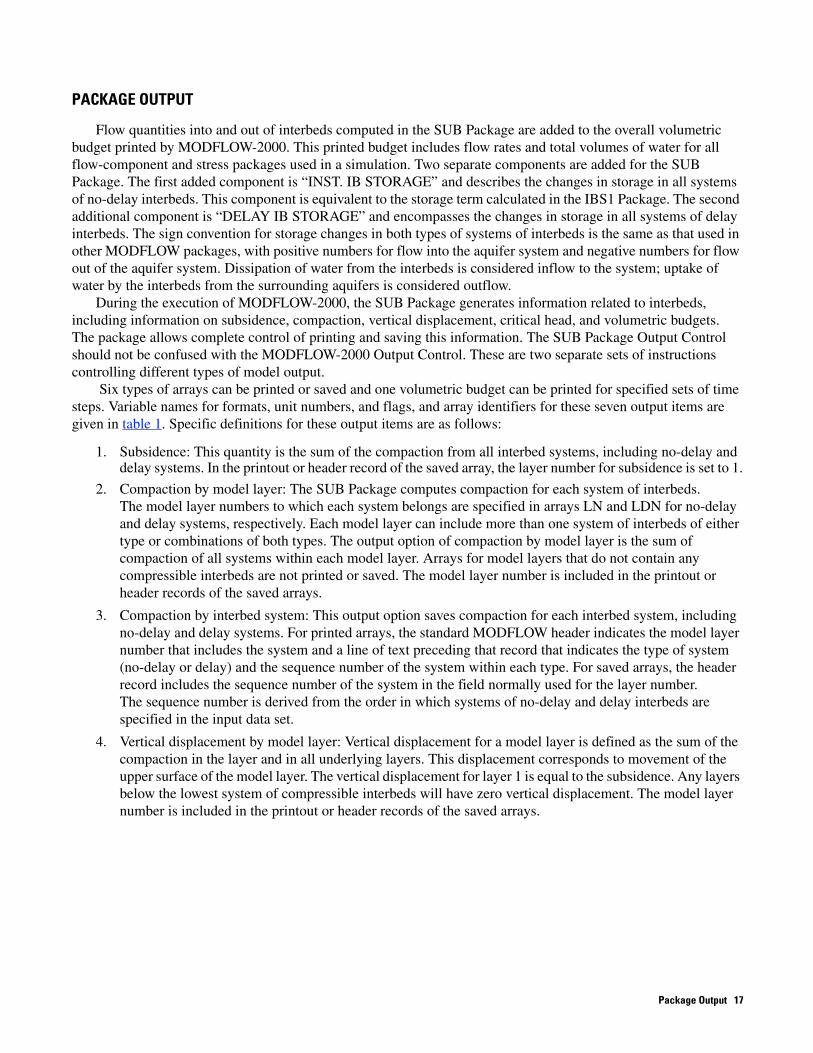
7. Volumetric budget for systems of delay interbeds: A volumetric budget for all active model cells is a fundamental part of the MODFLOW listing. The SUB Package, however, solves equations for systems of delay interbeds separately from the ground-water flow equations to which the MODFLOW volumetric budget applies. The package computes a separate volumetric budget for systems of delay interbeds (fig. 4). The volumetric interbed budget can be used to determine how well equations describing flow in interbeds are being solved. If possible, the discrepancy in the budget should be less than a few percent. The budget can be printed in the main MODFLOW listing file for selected time steps, but cannot be saved to a file.

Table 1. Information optionally printed or saved by the Subsidence and Aquifer-System Compaction Package and associated variable names, numbers of arrays, and array names.

Information printed or saved

Variable containing print format in input

data item 15

Variable containing unit number in in put

data item 15

Variable containing flag in data item 16 indicating print

action

Variable containing flag in data item 16 indicating save

action

Number of layer arrays that will

be saved each time step

Name of array as listed in printout and in

header record of saved array

Subsidence Ifm1 Iun1 Ifl1 Ifl2 1 SUBSIDENCE

Compaction by model layer

Ifm2 Iun2 Ifl3 Ifl4 One array for each layer with delay or no-delay interbeds

LAYER COMPACTION

Compaction by interbed system

Ifm3 Iun3 Ifl5 Ifl6 NNDB + NDB1 NDYS COMPACTION or DSYS COMPACTION

Vertical displacement by model layer

Ifm4 Iun4 Ifl7 Ifl8 NLAY1 Z DISPLACEMENT

Critical head for no-delay interbeds

Ifm5 Iun5 Ifl9 Ifl10 One array for each layer with no-delay interbeds

ND CRITICAL HEAD

Critical head for delay interbeds

Ifm6 Iun6 Ifl11 Ifl12 NDB1 D CRITICAL HEAD

Volumetric budget for delay interbeds

--- --- Ifl13 --- --- ---

1Defined in the section entitled “Input Instructions.”


VOLUMETRIC BUDGET FOR SYSTEMS OF INTERBEDS WITH DELAY PROPERTIES AT END OF TIME STEP 6 IN STRESS PERIOD 1

| C U M U L A T I V E V O L U M E S L**3 | R A T E S F O R T H I S T I M E S T E P L**3/T | SYSTEM | CHANGE IN BOUNDARY PERCENT | CHANGE IN BOUNDARY PERCENT | NUMBER | STORAGE FLOW SUM DISCREPANCY | STORAGE FLOW SUM DISCREPANCY | --------|--------------------------------------------------------|-------------------------------------------------------| 1 2683.0 -2683.0 -0.24414E-03 -0.90994E-05 10.762 -10.762 -0.19073E-05 -0.17723E-04 2 0.37168E+07 -0.37168E+07 0.25000 0.67262E-05 10515. -10515. -0.97656E-03 -0.92874E-05 --------|--------------------------------------------------------|-------------------------------------------------------| TOTALS: 0.37195E+07 -0.37195E+07 0.25000 0.67214E-05 10526. -10526. -0.97656E-03 -0.92779E-05

Figure 4. Example of volumetric budget for systems of delay interbeds.

The sign convention for subsidence and vertical displacement is positive for lowering and negative for uplift. The sign convention for compaction is positive for compression or shortening and negative for expansion. Numbers for critical head are referenced to the same datum used for head in the model. The sign convention for the volumetric budgets of delay interbeds is positive for release of water from storage and for boundary flow from aquifers into the interbeds, and negative for the opposite conditions.

By default, the first six output items will not be printed or saved to files, but item 7 will be printed in the main MODFLOW listing file for the final time step of all transient stress periods. If output different from the default is desired for any model time steps, records specifying alternative output must be included as repetitions of input data item 16 (see “Input Instructions”). The defaults plus ISUBOC (see “Explanation of Fields”) repetitions of item 16 define the SUB Package scheme using a series of flags stored in memory for every time step in every stress period in the simulation. Each repetition of item 16 sets flags that control output for a set of time steps, where the set is specified as a range of time steps in each stress period for a range of stress periods. The set of time steps is defined in each repetition of item 16 by four integers that specify (1) the starting stress period in the range of stress periods, (2) the ending stress period in the range of stress periods, (3) the starting time step in the range of time steps in each stress period to be included in the set, and (4) the ending time step in the range of time steps in each stress period to be included in the set. Following the integers that define the set of time steps, each record includes 12 integer flags that specify whether or not to print or save each of the first six output items and a thirteenth flag that specifies whether or not to print output item 7. If any time step is included in more than one repetition of item 16, the flags in later repetitions override those in earlier repetitions for that time step. If the number read for a flag to print or save a data item is negative, the default or previously set value of the flag for printing or saving the data item will remain unchanged. If the number read for a flag is zero, the flag for printing or saving will be set to not print or save. If the number read for a flag to print or save a data item is positive, the flag for printing or saving will be set to print or save.

For each repetition of input data item 16, the set of time steps to which flags for printing and storing data items are applied is defined using the following rules:

1. Any starting or ending stress period or time step that is specified to be less than 1 will be reset to 1.2. Any starting or ending stress period that is specified to be greater than the total number of stress periods in

the simulation (NPER) will be reset to NPER.

3. Any starting or ending time step that is specified to be greater than the total number of time steps in a particular stress period [NSTP(N) for stress period N] will be reset to NSTP(N).

4. Any ending stress period that is specified to be less than the corresponding starting stress period will be reset to the starting stress period.

5. Any ending time step that is specified to be less than the corresponding starting time step will be reset to the starting time step.

6. For the resulting range of stress periods, each time step within the resulting range of time steps will have the flags for printing or saving set as specified.

Package Output 19

The following example will help in understanding this system. Suppose that a simulation includes five stress periods, containing twelve time steps in the first, second and third, and six time steps in the fourth and fifth. Further suppose that the desired output is (a) subsidence printed to the listing file (flag Ifl1) for the last time step in each of the five stress periods, (b) compaction by model layer saved to a file (flag Ifl4) for all time steps in all stress periods, and (c) volumetric budget of delay interbeds printed for the last time step in each stress period (the default condition). These actions could be specified with two repetitions of input data item 16:

1 5 12 12 1 -2 -2 -2 -2 -2 -2 -2 -2 -2 -2 -2 -2

1 5 1 12 -2 -2 -2 1 -2 -2 -2 -2 -2 -2 -2 -2 -2

Note that the range of time steps for stress periods 4 and 5 will be reset to go from 1 to 6 because each of these has only 6 time steps. Also note that, for this example, the same output could be obtained by reversing the order of the two repetitions of input data item 16.

In addition to the output items specified above, the SUB Package can save cell-by-cell flow terms to files in the manner that similar terms are saved for other flow-related packages. Terms are written to a file associated with the unit number specified by variable ISUBCB (see “Explanation of Fields”) for time steps when “SAVE BUDGET” or a non-zero value of variable ICBCFL (flag for writing cell-by-cell flow data) is specified in the MODFLOW-2000 Output Control file (Harbaugh and others, 2000, p. 52). If no-delay interbeds are simulated, cell-by-cell terms for rates of storage change in these beds will be written using the name “INTERBED STORAGE” in the header record. Similarly, if delay interbeds are simulated, cell-by-cell terms for rates of storage change in these beds will be written using the name “DELAYED STORAGE” in the header record.


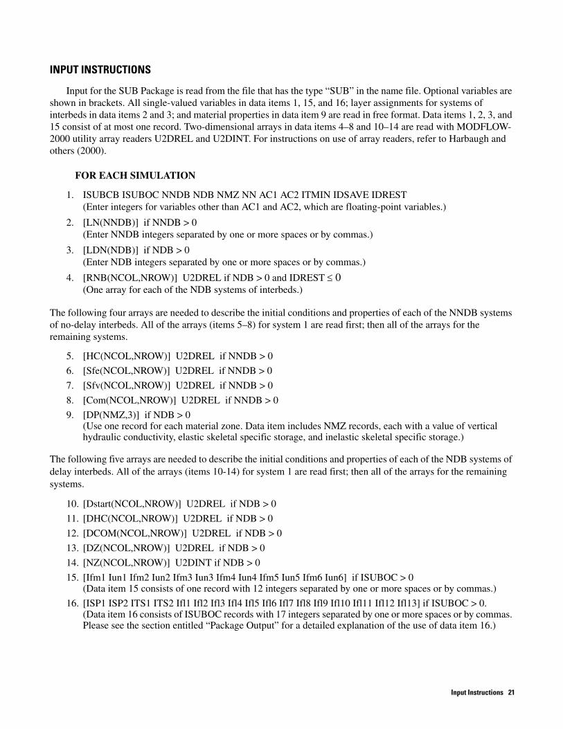
INPUT INSTRUCTIONS

Input for the SUB Package is read from the file that has the type “SUB” in the name file. Optional variables are shown in brackets. All single-valued variables in data items 1, 15, and 16; layer assignments for systems of interbeds in data items 2 and 3; and material properties in data item 9 are read in free format. Data items 1, 2, 3, and 15 consist of at most one record. Two-dimensional arrays in data items 4–8 and 10–14 are read with MODFLOW-2000 utility array readers U2DREL and U2DINT. For instructions on use of array readers, refer to Harbaugh and others (2000).

FOR EACH SIMULATION

1. ISUBCB ISUBOC NNDB NDB NMZ NN AC1 AC2 ITMIN IDSAVE IDREST (Enter integers for variables other than AC1 and AC2, which are floating-point variables.)

2. [LN(NNDB)] if NNDB > 0 (Enter NNDB integers separated by one or more spaces or by commas.)

3. [LDN(NDB)] if NDB > 0 (Enter NDB integers separated by one or more spaces or by commas.)

4. [RNB(NCOL,NROW)] U2DREL if NDB > 0 and IDREST ≤ 0 (One array for each of the NDB systems of interbeds.)

The following four arrays are needed to describe the initial conditions and properties of each of the NNDB systems of no-delay interbeds. All of the arrays (items 5–8) for system 1 are read first; then all of the arrays for the remaining systems.

5. [HC(NCOL,NROW)] U2DREL if NNDB > 0

6. [Sfe(NCOL,NROW)] U2DREL if NNDB > 0

7. [Sfv(NCOL,NROW)] U2DREL if NNDB > 0

8. [Com(NCOL,NROW)] U2DREL if NNDB > 0

9. [DP(NMZ,3)] if NDB > 0 (Use one record for each material zone. Data item includes NMZ records, each with a value of vertical hydraulic conductivity, elastic skeletal specific storage, and inelastic skeletal specific storage.)

The following five arrays are needed to describe the initial conditions and properties of each of the NDB systems of delay interbeds. All of the arrays (items 10-14) for system 1 are read first; then all of the arrays for the remaining systems.

10. [Dstart(NCOL,NROW)] U2DREL if NDB > 0

11. [DHC(NCOL,NROW)] U2DREL if NDB > 0

12. [DCOM(NCOL,NROW)] U2DREL if NDB > 0

13. [DZ(NCOL,NROW)] U2DREL if NDB > 0

14. [NZ(NCOL,NROW)] U2DINT if NDB > 0

15. [Ifm1 Iun1 Ifm2 Iun2 Ifm3 Iun3 Ifm4 Iun4 Ifm5 Iun5 Ifm6 Iun6] if ISUBOC > 0 (Data item 15 consists of one record with 12 integers separated by one or more spaces or by commas.)

16. [ISP1 ISP2 ITS1 ITS2 Ifl1 Ifl2 Ifl3 Ifl4 Ifl5 Ifl6 Ifl7 Ifl8 Ifl9 Ifl10 Ifl11 Ifl12 Ifl13] if ISUBOC > 0. (Data item 16 consists of ISUBOC records with 17 integers separated by one or more spaces or by commas. Please see the section entitled “Package Output” for a detailed explanation of the use of data item 16.)

Input Instructions 21

Explanation of Fields Used in Input Instructions

ISUBCB is a flag and unit number.

If ISUBCB > 0, it is the unit number to which cell-by-cell flow terms will be written when “SAVE BUDGET” or a non-zero value for ICBCFL is specified in MODFLOW-2000 Output Control (see Harbaugh and others, 2000, p. 52–55).

If ISUBCB ≤ 0, cell-by-cell flow terms will not be recorded.

ISUBOC is a flag used to control output of information generated by the SUB Package.

If ISUBOC > 0, it is the number of repetitions of item 16 to be read, each repetition of which defines a set of times steps and associated flags for printing and saving subsidence, compaction, vertical displacement, preconsolidation head, and volumetric budget.

If ISUBOC ≤ 0, volumetric budgets for systems of delay interbeds will be printed at the end of each stress period. Subsidence, compaction, vertical displacement, and preconsolidation head will not be printed or saved.

NNDB is the number of systems of no-delay interbeds.

NDB is the number of systems of delay interbeds.

NMZ is the number of material zones that are needed to define the hydraulic properties of systems of delay interbeds. Each material zone is defined by a combination of vertical hydraulic conductivity, elastic systems of delay interbeds.

NN is the number of nodes used to discretize the half space to approximate the head distributions in systems of delay interbeds.

AC1 is an acceleration parameter. This parameter (ω1 in equation 25) is used to predict the aquifer head at the interbed boundaries on the basis of the head change computed for the previous iteration. A value of 0.0 results in the use of the aquifer head at the previous iteration. Limited experience indicates that optimum values may range from 0.0 to 0.6.

AC2 is an acceleration parameter. This acceleration parameter is a multiplier for the head changes to compute the head at the new iteration (ω2 in equation 27). Values are normally between 1.0 and 2.0, but the optimum probably is closer to 1.0 than to 2.0. As discussed following equation 27, however, this parameter also can be used to help convergence of the iterative solution by using values between 0 and 1.

ITMIN is the minimum number of iterations for which one-dimensional equations will be solved for flow in interbeds when the Strongly Implicit Procedure (SIP) is used to solve the ground-water flow equations. If the current iteration level is greater than ITMIN and the SIP convergence criterion for head closure (HCLOSE) is met at a particular cell, the one-dimensional equations for that cell will not be solved. The previous solution will be used. The value of ITMIN is read but not used if a solver other than SIP is used to solve the ground-water flow equations.

IDSAVE is a flag and a unit number.

If IDSAVE > 0, it is the unit number on which restart records for delay interbeds will be saved at the end of the simulation. The unit number must be associated with a BINARY data file specified in the MODFLOW Name File.

If IDSAVE ≤ 0, restart records for delay interbeds will not be saved.


IDREST is a flag and a unit number.

If IDREST > 0, it is the unit number on which restart records for delay interbeds will be read at the start of the simulation. The unit number must be associated with a BINARY data file specified in the MODFLOW Name File.

If IDREST ≤ 0, restart records for delay interbeds will not be read.

LN is a one-dimensional array specifying the model layer assignments for each system of no-delay interbeds. The array has NNDB values.

LDN is a one-dimensional array specifying the model layer assignments for each system of delay interbeds. The array has NDB values.

RNB is an array specifying the factor nequiv (eq. 20) at each cell for each system of delay interbeds. The array also is used to define the areal extent of each system of interbeds. For cells beyond the areal extent of the system of interbeds, enter a number less than 1.0 in the corresponding element of this array.

HC is an array specifying the preconsolidation head or preconsolidation stress in terms of head in the aquifer for systems of no-delay interbeds. For any model cells in which specified HC is greater than the corresponding value of starting head, the value of HC will be set to that of starting head.

Sfe is an array specifying the dimensionless elastic skeletal storage coefficient for systems of no-delay interbeds. Values may be estimated using equation 17.

Sfv is an array specifying the dimensionless inelastic skeletal storage coefficient for systems of no-delay interbeds. Values may be estimated using equation 17.

COM is an array specifying the starting compaction in each system of no-delay interbeds. Compaction values computed by the package are added to values in this array so that printed or stored values of compaction and land subsidence may include previous components. Values in this array do not affect calculations of storage changes or resulting compaction. For simulations in which output values are to reflect compaction and subsidence since the start of the simulation, enter zero values for all elements of this array.

DP is an array containing a table of material properties for systems of delay interbeds. For each of the NMZ zones of material properties, vertical hydraulic conductivity, elastic skeletal specific storage, and inelastic skeletal specific storage are read.

Dstart is an array specifying starting head in interbeds for systems of delay interbeds. For a particular location in a system of interbeds, the starting head is applied to every node in the string of nodes that approximates flow in half of a doubly draining interbed.

DHC is an array specifying the starting preconsolidation head in interbeds for systems of delay interbeds. For a particular location in a system of interbeds, the starting preconsolidation head is applied to every node in the string of nodes that approximates flow in half of a doubly draining interbed. For any location at which specified starting preconsolidation head is greater than the corresponding value of the starting head, Dstart, the value of the starting preconsolidation head will be set to that of the starting head.

DCOM is an array specifying the starting compaction in each system of delay interbeds. Compaction values computed by the package are added to values in this array so that printed or stored values of compaction and land subsidence may include previous components. Values in this array do not affect calculations of storage changes or resulting compaction. For simulations in which output values are to reflect compaction and subsidence since the start of the simulation, enter zero values for all elements of this array.


DZ is an array specifying the equivalent thickness for a system of delay interbeds (bequiv in equation 19).

NZ is an array specifying the material zone numbers for systems of delay interbeds. The zone number for each location in the model grid selects the hydraulic conductivity, elastic skeletal specific storage, and inelastic skeletal specific storage of the interbeds.

Ifm1 is a code for the format in which subsidence will be printed. Format codes for variables Ifm1, Ifm2, Ifm3, Ifm4, Ifm5, Ifm6 are as follows:

0 - (10G11.4) 7 - (20F5.0)1 - (11G10.3) 8 - (20F5.1)2 - (9G13.6) 9 - (20F5.2)3 - (15F7.1) 10 - (20F5.3)4 - (15F7.2) 11 - (20F5.4)5 - (15F7.3) 12 - (10G11.4)6 - (15F7.4)

Iun1 is the unit number to which subsidence will be written if it is saved on disk.

Ifm2 is a code for the format in which compaction by model layer will be printed.

Iun2 is the unit number to which compaction by model layer will be written if it is saved on disk.

Ifm3 is a code for the format in which compaction by interbed system will be printed.

Iun3 is the unit number to which compaction by interbed system will be written if it is saved on disk.

Ifm4 is a code for the format in which vertical displacement will be printed.

Iun4 is the unit number to which vertical displacement will be written if it is saved on disk.

Ifm5 is a code for the format in which no-delay preconsolidation head will be printed.

Iun5 is the unit number to which no-delay preconsolidation head will be written if it is saved on disk.

Ifm6 is a code for the format in which delay preconsolidation head will be printed.

Iun6 is the unit number to which delay preconsolidation head will be written if it is saved on disk.

The variables ISP1, ISP2, ITS1, ITS2, and Ifl1 through Ifl13 are used to control printing and saving of information generated by the SUB Package during program execution. The use of some of these variables is explained in more detail in the section entitled Package Output. The default condition for flags Ifl1 through Ifl13 is to not print or save the indicated information, except for printing budgets for no-delay interbeds for the last time step of each stress period.

ISP1 is the starting stress period in the range of stress periods to which output flags Ifl1 through Ifl13 apply. If the value of ISP1 is less than 1, the SUB Package will change the number to 1.

ISP2 is the ending stress period in the range of stress periods and time steps to which output flags Ifl1 through Ifl13 apply. If the value of ISP1 is greater than NPER (the number of stress periods in the simulation), the SUB Package will change the number to NPER.

ITS1 is the starting time step in the range of time steps in each of the stress periods ISP1 through ISP2 to which output flags Ifl1 through Ifl13 apply. If the value of ITS1is less than 1, the SUB Package will change the number to 1.


ITS2 is the ending time step in the range of time steps in each of stress periods ISP1 through ISP2 to which output flags Ifl1 through Ifl13 apply. If the value of ITS2 is greater than the number of time steps in a given stress period, the SUB Package will change the number to the number of time steps in that stress period.

Ifl1 is the output flag for printing subsidence for the set of time steps specified by ISP1, ISP2, ITS1, and ITS2.

If Ifl1 < 0, use default or previously defined settings of Ifl1 for printing subsidence.If Ifl1 = 0, do not print subsidence.If Ifl1 > 0, print subsidence.

Ifl2 is the output flag for saving subsidence to an unformatted disk file for the set of time steps specified by ISP1, ISP2, ITS1, and ITS2.

If Ifl2 < 0, use default or previously defined settings of Ifl2 for saving subsidence.If Ifl2 = 0, do not save subsidence.If Ifl2 > 0, save subsidence.

Ifl3 is the output flag for printing compaction by model layer for the set of time steps specified by ISP1, ISP2, ITS1, and ITS2.

If Ifl3 < 0, use default or previously defined settings of Ifl3 for printing compaction by model layer.If Ifl3 = 0, do not print compaction by model layer.If Ifl3 > 0, print compaction by model layer.

Ifl4 is the output flag for saving compaction by model layer to an unformatted disk file for the set of time steps specified by ISP1, ISP2, ITS1, and ITS2.

If Ifl4 < 0, use default or previously defined settings of Ifl4 for saving compaction by model layer.If Ifl4 = 0, do not save compaction by model layer.If Ifl4 > 0, save compaction by model layer.

Ifl5 is the output flag for printing compaction by interbed system for the set of time steps specified by ISP1, ISP2, ITS1, and ITS2.

If Ifl5 < 0, use default or previously defined settings of Ifl5 for printing compaction by interbed system.If Ifl5 = 0, do not print compaction by interbed system.If Ifl5 > 0, print compaction by interbed system.

Ifl6 is the output flag for saving compaction by interbed system to an unformatted disk file for the set of time steps specified by ISP1, ISP2, ITS1, and ITS2.

If Ifl6 < 0, use default or previously defined settings of Ifl6 for saving compaction by interbed system.If Ifl6 = 0, do not save compaction by interbed system.If Ifl6 > 0, save compaction by interbed system.

Ifl7 is the output flag for printing vertical displacement for the set of time steps specified by ISP1, ISP2, ITS1, and ITS2.

If Ifl7 < 0, use default or previously defined settings of Ifl7 for printing vertical displacement.If Ifl7 = 0, do not print vertical displacement.If Ifl7 > 0, print vertical displacement.


Ifl8 is the output flag for saving vertical displacement to an unformatted disk file for the set of time steps specified by ISP1, ISP2, ITS1, and ITS2.

If Ifl8 < 0, use default or previously defined settings of Ifl8 for saving vertical displacement.If Ifl8 = 0, do not save vertical displacement.If Ifl8 > 0, save vertical displacement.

Ifl9 is the output flag for printing critical head for no-delay interbeds for the set of time steps specified by ISP1, ISP2, ITS1, and ITS2.

If Ifl9 < 0, use default or previously defined settings of Ifl9 for printing critical head for no-delay interbeds.If Ifl9 = 0, do not print critical head for no-delay interbeds.If Ifl9 > 0, print critical head for no-delay interbeds.

Ifl10 is the output flag for saving critical head for no-delay interbeds to an unformatted disk file for the set of time steps specified by ISP1, ISP2, ITS1, and ITS2.

If Ifl10 < 0, use default or previously defined settings of Ifl10 for saving critical head for no-delay interbeds.If Ifl10 = 0, do not save critical head for no-delay interbeds.If Ifl10 > 0, save critical head for no-delay interbeds.

Ifl11 is the output flag for printing critical head for delay interbeds for the set of time steps specified by ISP1, ISP2, ITS1, and ITS2.

If Ifl11 < 0, use default or previously defined settings of Ifl11 for printing critical head for delay interbeds.If Ifl11 = 0, do not print critical head for delay interbeds.If Ifl11 > 0, print critical head for delay interbeds.

Ifl12 is the output flag for saving critical head for delay interbeds to an unformatted disk file for the set of time steps specified by ISP1, ISP2, ITS1, and ITS2.

If Ifl12 < 0, use default or previously defined settings of Ifl12 for saving critical head for delay interbeds.If Ifl12 = 0, do not save critical head for delay interbeds.If Ifl12 > 0, save critical head for delay interbeds.

Ifl13 is the output flag for printing volumetric budget for delay interbeds for the set of time steps specified by ISP1, ISP2, ITS1, and ITS2.

If Ifl13 < 0, use default or previously defined settings of Ifl13 for printing volumetric budget for delay interbeds.If Ifl13 = 0, do not print volumetric budget for delay interbeds.If Ifl13 > 0, print volumetric budget for delay interbeds.


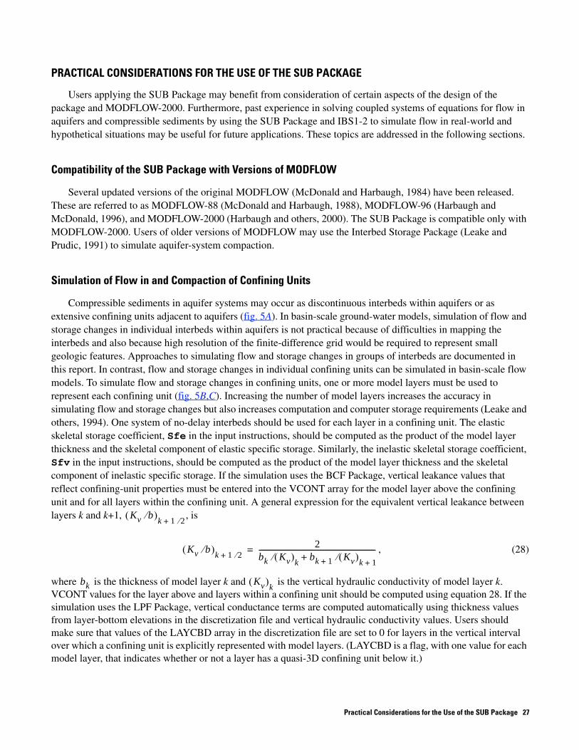
PRACTICAL CONSIDERATIONS FOR THE USE OF THE SUB PACKAGE

Users applying the SUB Package may benefit from consideration of certain aspects of the design of the package and MODFLOW-2000. Furthermore, past experience in solving coupled systems of equations for flow in aquifers and compressible sediments by using the SUB Package and IBS1-2 to simulate flow in real-world and hypothetical situations may be useful for future applications. These topics are addressed in the following sections.

Compatibility of the SUB Package with Versions of MODFLOW

Several updated versions of the original MODFLOW (McDonald and Harbaugh, 1984) have been released. These are referred to as MODFLOW-88 (McDonald and Harbaugh, 1988), MODFLOW-96 (Harbaugh and McDonald, 1996), and MODFLOW-2000 (Harbaugh and others, 2000). The SUB Package is compatible only with MODFLOW-2000. Users of older versions of MODFLOW may use the Interbed Storage Package (Leake and Prudic, 1991) to simulate aquifer-system compaction.

Simulation of Flow in and Compaction of Confining Units

Compressible sediments in aquifer systems may occur as discontinuous interbeds within aquifers or as extensive confining units adjacent to aquifers (fig. 5A). In basin-scale ground-water models, simulation of flow and storage changes in individual interbeds within aquifers is not practical because of difficulties in mapping the interbeds and also because high resolution of the finite-difference grid would be required to represent small geologic features. Approaches to simulating flow and storage changes in groups of interbeds are documented in this report. In contrast, flow and storage changes in individual confining units can be simulated in basin-scale flow models. To simulate flow and storage changes in confining units, one or more model layers must be used to represent each confining unit (fig. 5B,C). Increasing the number of model layers increases the accuracy in simulating flow and storage changes but also increases computation and computer storage requirements (Leake and others, 1994). One system of no-delay interbeds should be used for each layer in a confining unit. The elastic skeletal storage coefficient, Sfe in the input instructions, should be computed as the product of the model layer thickness and the skeletal component of elastic specific storage. Similarly, the inelastic skeletal storage coefficient, Sfv in the input instructions, should be computed as the product of the model layer thickness and the skeletal component of inelastic specific storage. If the simulation uses the BCF Package, vertical leakance values that reflect confining-unit properties must be entered into the VCONT array for the model layer above the confining unit and for all layers within the confining unit. A general expression for the equivalent vertical leakance between layers k and k+1, Kv b⁄( )k 1 2⁄+

, is

Kv b⁄( )k 1 2⁄+2

bk Kv( )k⁄ bk 1+ Kv( )k 1+⁄+

-------------------------------------------------------------------= , (28)

where bk is the thickness of model layer k and Kv( )k is the vertical hydraulic conductivity of model layer k. VCONT values for the layer above and layers within a confining unit should be computed using equation 28. If the simulation uses the LPF Package, vertical conductance terms are computed automatically using thickness values from layer-bottom elevations in the discretization file and vertical hydraulic conductivity values. Users should make sure that values of the LAYCBD array in the discretization file are set to 0 for layers in the vertical interval over which a confining unit is explicitly represented with model layers. (LAYCBD is a flag, with one value for each model layer, that indicates whether or not a layer has a quasi-3D confining unit below it.)

Practical Considerations for the Use of the SUB Package 27

Aquifer withcompressiblefine-grained

interbeds

Modellayer

A.

Intermediateconfining unit

B.

1

7

4

5

6

3

2

1

Modellayer

C.

3

2

Upper aquifer

Lower aquifer

Aquifer withcompressiblefine-grained

interbeds

Compressiblefine-grained

confining unit

Figure 5. Compressible beds in an aquifer system and two approaches to representing the confining unit in the MODFLOW simulation of aquifer-system compaction using the SUB Package. A, Vertical section of an aquifer system with compressible sediments within and adjacent to aquifers. B, Use of one model layer to simulate flow and storage changes in the confining unit C, Use of five model layers to simulate flow and storage changes in the confining unit.

Use of Steady-State Stress Periods in MODFLOW-2000

In MODFLOW-2000, each stress period may be either steady-state or transient. The ability to mix steady-state and transient stress periods in a single simulation allows users to set up an initial steady-state stress period that simulates predevelopment conditions and subsequent stress periods that simulate transient post-development conditions (see sample problem 3). The SUB Package need not make any calculations in steady-state stress periods, but the heads calculated by the model for a steady-state stress period are relevant to calculations made by the package for subsequent transient stress periods. When steady-state and transient stress periods are mixed in a simulation, the SUB Package operates in the following manner:

1. If any stress periods other than the first are steady-state, the SUB Package prints a message in the listing file and aborts the simulation. Simulations are allowed in which the first stress period is steady-state and subsequent stress periods are transient or in which all stress periods are transient.

2. At the end of the first (steady-state) stress period, starting preconsolidation heads for all interbeds in the HC and DHC arrays are reset to the calculated steady-state head for any cell in which the head computed in the first stress period is below the corresponding value of preconsolidation head.

3. At the end of the first stress period, starting head for delay interbeds in the Dstart array are reset to the calculated steady-state head computed in the first stress period at corresponding model cells. Values read into the Dstart array in the SUB Package input are not used.

4. Starting compaction values in the COM and DCOM arrays are not modified to incorporate changes in conditions resulting from a steady-state stress period.


Improvement of Convergence in Solutions of Coupled Equations

When the SUB Package is included in a MODFLOW-2000 simulation, and delay interbeds are used, the systems of equations describing the diffusion process from the interbeds (eq. 21) are coupled to the system of equations describing three-dimensional ground-water flow (finite-difference approximations of equation 15). The two systems are coupled through common flow terms. Both systems of equations are solved iteratively at every time step and must converge to a common solution. When and where water from delayed drainage of interbeds constitutes a major source of water in a MODFLOW model cell, the iteratively determined aquifer head at the end of the time step may fluctuate around the solution and sometimes fail to converge to a final value. This numerical problem is the result of solving the two systems of equations in a coupled way rather than combining them into a single system and solving that system. If such convergence problems are encountered in a simulation, two actions can alleviate the problem. First, transferring storage from delay interbeds to no-delay interbeds stabilizes the convergence significantly. Typically, convergence problems only occur if the volume of water derived from delay interbeds is much larger than that from no-delay interbeds or other sources and sinks in a cell. Thus, interbeds should be conceptualized as no-delay interbeds where possible. If the modeled aquifer has interbeds of varying thickness, the thinnest interbeds that drain the most rapidly can be combined into a system no-delay interbeds and the remaining interbeds can be represented by a system of delay interbeds. Second, the acceleration parameter AC2 (see input instructions, ω2 in equation 27) can be set to values between 0 and 1 to dampen the iterative solution and help convergence. The optimal value of this parameter is problem dependent. Small values will result in slower convergence as more iterations are performed at every time step, while large values may result in a failure to converge at a time step.

SAMPLE SIMULATIONS

In order to demonstrate the validity, applicability, and capabilities of the SUB Package, two simple one-dimensional simulations and a third more complex simulation are shown. An example of the SUB input data sets for sample problem 3 are presented in the Appendix.

Sample Problem 1

The first test problem simulates the drainage of a thick interbed caused by a step decrease in hydraulic head in the aquifer. The representation of this scenario in a model is shown in figure 6A. Two constant-head cells bound the cell containing the interbed. The water released from the interbed during the simulation can leave the system through these cells. The transmissivity in the aquifer was set to a very large value, so that the head in the aquifer in the center cell remains constant. The time constant, τ0 (eq. 14), was chosen to be 1,000 with vertical hydraulic conductivity set to 0.025, interbed thickness set to 1, and elastic skeletal specific storage set to 1 and inelastic skeletal specific storage set to 100. Units are not shown for these values, as any consistent set of length and time units results in the same solution. Ten finite-difference nodes represent the half-thickness of the interbed (NN in input instructions). The initial head in the center cell and the specified heads in the constant-head cells were identical. The starting head and the preconsolidation head in the interbed were specified one unit higher than the head in the surrounding aquifer. The resulting compaction of the interbed is compared to the theoretical solution (derived using equations 9, 12, and 14) in figure 6B,C. The SUB-computed values closely match the theoretical values. The small differences, particularly at early times, may be at least partly due to the fact that the aquifer head in the simulation does not remain exactly constant as a result of water entering the aquifer from the interbed. Because of the finite transmissivity of the aquifer, the head in the aquifer briefly rises to about 2 percent of the starting head in the interbed during the first time step.

Sample Simulations 29

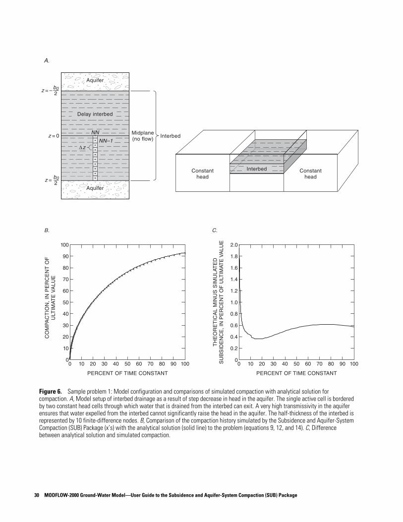
Midplane(no flow)

Constanthead

Constanthead

Aquifer

A.

Delay interbed

Interbed

Interbed

Aquifer

NN

NN–1z = 0

∆z

CO

MPA

CT

ION

, IN

PE

RC

EN

T O

FU

LTIM

ATE

VA

LU

E

100

90

80

70

030 40 50 60 70 80 100900

PERCENT OF TIME CONSTANT

60

50

40

30

20

10

2010

C.B.

TH

EO

RE

TIC

AL

MIN

US

SIM

ULA

TE

DS

UB

SID

EN

CE

, IN

PE

RC

EN

T O

F U

LTIM

ATE

VA

LUE 2.0

1.8

1.6

1.4

030 40 50 60 70 80 100900

PERCENT OF TIME CONSTANT

1.2

1.0

0.8

0.6

0.4

0.2

2010

z = – b02

z = b02


Figure 6. Sample problem 1: Model configuration and comparisons of simulated compaction with analytical solution for compaction. A, Model setup of interbed drainage as a result of step decrease in head in the aquifer. The single active cell is bordered by two constant head cells through which water that is drained from the interbed can exit. A very high transmissivity in the aquifer ensures that water expelled from the interbed cannot significantly raise the head in the aquifer. The half-thickness of the interbed is represented by 10 finite-difference nodes. B, Comparison of the compaction history simulated by the Subsidence and Aquifer-System Compaction (SUB) Package (x’s) with the analytical solution (solid line) to the problem (equations 9, 12, and 14). C, Difference between analytical solution and simulated compaction.

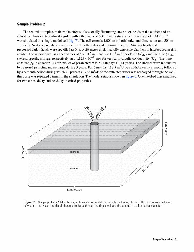
Sample Problem 2

The second example simulates the effects of seasonally fluctuating stresses on heads in the aquifer and on subsidence history. A confined aquifer with a thickness of 500 m and a storage coefficient (S) of 1.44 × 10-3 was simulated in a single model cell (fig. 7). The cell extends 1,000 m in both horizontal dimensions and 500 m vertically. No-flow boundaries were specified on the sides and bottom of the cell. Starting heads and preconsolidation heads were specified as 0 m. A 20-meter thick, laterally extensive clay lens is interbedded in this aquifer. The interbed was assigned values of 5 × 10–5 m–1 and 5 × 10–3 m–1 for elastic (S′ske) and inelastic (S′skv) skeletal specific storage, respectively, and 1.125 × 10–10 m/s for vertical hydraulic conductivity (K′v). The time constant (τ0 in equation 14) for this set of parameters was 51,440 days (~141 years). The stresses were modulated by seasonal pumping and recharge during 5 years: For 6 months, 118.3 m3/d was withdrawn by pumping followed by a 6-month period during which 20 percent (23.66 m3/d) of the extracted water was recharged through the well; this cycle was repeated 5 times in the simulation. The model setup is shown in figure 7. One interbed was simulated for two cases, delay and no-delay interbed properties.

20

Me

ters

50

0 M

ete

rs

Interbed

1,000 Meters

1,000 M

eters

Aquifer

Recharge

Dis

char

ge


Figure 7. Sample problem 2: Model configuration used to simulate seasonally fluctuating stresses. The only sources and sinks of water in the system are the discharge or recharge through the single well and the storage in the interbed and aquifer.

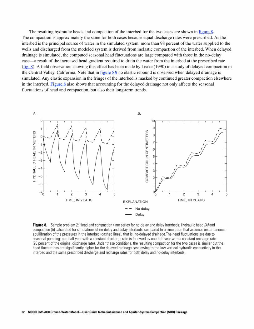
The resulting hydraulic heads and compaction of the interbed for the two cases are shown in figure 8. The compaction is approximately the same for both cases because equal discharge rates were prescribed. As the interbed is the principal source of water in the simulated system, more than 98 percent of the water supplied to the wells and discharged from the modeled system is derived from inelastic compaction of the interbed. When delayed drainage is simulated, the computed seasonal head fluctuations are large compared with those in the no-delay case—a result of the increased head gradient required to drain the water from the interbed at the prescribed rate (fig. 8). A field observation showing this effect has been made by Leake (1990) in a study of delayed compaction in the Central Valley, California. Note that in figure 8B no elastic rebound is observed when delayed drainage is simulated. Any elastic expansion in the fringes of the interbed is masked by continued greater compaction elsewhere in the interbed. Figure 8 also shows that accounting for the delayed drainage not only affects the seasonal fluctuations of head and compaction, but also their long-term trends.

A.

HY

DR

AU

LIC

HE

AD

, IN

ME

TE

RS

2

1

0

2 3 4 50

TIME, IN YEARS

–1

–2

–3

–4

–5

–6

1

B.

CO

MPA

CT

ION

, IN

CE

NT

IME

TE

RS

10

9

8

7

02 3 4 50

TIME, IN YEARSEXPLANATION

No delay

Delay

6

5

4

3

2

1

1–7


Figure 8. Sample problem 2: Head and compaction time series for no-delay and delay interbeds. Hydraulic head (A) and compaction (B) calculated for simulations of no-delay and delay interbeds. compared to a simulation that assumes instantaneous equilibration of the pressures in the interbed (dashed lines), that is, no-delayed drainage.The head fluctuations are due to seasonal pumping: one-half year with a constant discharge rate is followed by one-half year with a constant recharge rate (20 percent of the original discharge rate). Under these conditions, the resulting compaction for the two cases is similar but the head fluctuations are significantly higher for the delayed drainage case owing to the low vertical hydraulic conductivity in the interbed and the same prescribed discharge and recharge rates for both delay and no-delay interbeds.

Sample Problem 3

To demonstrate a three-dimensional application of the SUB Package including the required input files, a more realistic, albeit simple, test problem is presented. Head decline and compaction of compressible interbeds were computed for simulated pumping from a hypothetical ground-water basin (fig. 9). The model has three layers that are 100 m, 50 m and 200 m thick. The basin has an overall extent of 10 km by 20 km (fig. 9A). The bottom boundary was simulated as impermeable bedrock. The top and bottom model layers (upper and lower aquifers in fig. 9B) consisted of unconsolidated fine- and coarse-grained sediments. For these two layers, the coarse-grained sediments constituted 40 percent of the thickness; fine-grained sediments made up the remaining 60 percent.

22

1

3

2

0

100

150

0 2 KILOMETERS 350

DE

PT

H B

EL

OW

LA

ND

SU

RFA

CE

, IN

ME

TE

RS

Confining unit

A.

B.

2221

19

18

17

16

15

14

13

12

10

98

76543

1

11

20

Column number

Row

nu

mb

er

1

1

2

3

4

5

6

7

8

9

10

2 3 4 5 6 7 8 9 10

MODEL GRID

VERTICAL SECTIONModelLayer

EXPLANATION

Discharge area (layer 1)

Recharge area (layer 1)

Line of equal head prior to pumping (layer 1), interval 1 meter

Pumping well (layer 3)

Location of heads and subsidence

10

2

Upper aquifer

Lower aquifer


Figure 9. Sample problem 3: Hypothetical ground-water basin. A, A plan view of a ground-water basin showing contours of head prior to pumping in the uppermost layer (layer 1). B, Vertical cross section showing aquifers, confining unit, and model layer designations.

The middle layer was a confining unit consisting only of fine-grained sediments except at the boundaries where it consisted of 50 percent coarse-grained sediments. For the coarse-grained sediments that constitute 40 percent of the top and bottom (aquifer) layers, skeletal storage coefficients were computed using the thicknesses of the sediments and values of elastic and inelastic skeletal specific storage, Sske = Sskv = 3×10–6 m–1. This assumes that deforma-tion of the coarse-grained sediments is elastic and allows for calculation of the compaction and (or) expansion of these sediments by the SUB Package. Properties specified for the fine-grained sediments are summarized in table 2. A vertical leakance value of 3 × 10–6 m–1 was specified in the VCONT array for all cells in the upper two model layers. A reference datum of zero was specified at land surface, which was idealized as perfectly flat.

Table 2. Hydrologic properties of the fine-grained sediments used in sample problem 3: [elastic skeletal specific storage (S’ske), inelastic skeletal specific storage (S′skv), and vertical hydraulic conductivity (K′v)]

Sske (per meter)

Sskv (per meter)

K′v (meters per day)

Layer 1 6 x 10-6 6 x 10-4 1 x 10-6

Layer 2 3 x 10-6 3 x 10-4 7.5 x 10-5

Layer3 6 x 10-6 6 x 10-4 1 x 10-6

On the basis of hypothetical data from lithologic and geophysical logs of wells in the basin, a number of interbeds of varying thicknesses in layers 1 and 3 were identified. Table 3 gives the individual thicknesses of the thicker interbeds. A number of relatively thin interbeds also were specified in both layers. The total thickness of these thin interbeds also is given in table 3. Table 3. Thickness of individual interbeds thicker than 1.5 m in layers 1 and 3 of sample problem 3 [The time constant, equivalent thickness, and the factor were calculated using equations 14, 19, and 20, respectively]

Thickness of individual

interbeds thicker than 1.5 meters,

in meters

Total thickness of all interbeds

thicker than 1.5 meters

Total thickness of all interbeds

thinner than 1.5 meters

Total thickness of all interbeds,

in metersTime constantτ0,

in days

Equivalent thickness bequiv, in

meters Factor, nequiv

Layer 1

2.1, 4.7, 7.7, 6.7, 4.5, 5.6, 7.8, 5.9

45 15 60 5,211.4 5,894 7,635

Layer 2

3.0, 2.2, 6.3, 6.4, 2.3, 7.6, 7.0, 7.0, 5.0, 7.2, 5.3, 5.7, 3.0, 3.2, 5.4, 3.6, 1.9, 4.7, 3.2

90 30 120 3,870.5 5,080 17.718

One system of no-delay interbeds was assigned to each of the three model layers (table 4) and one system of delay interbeds was assigned to the top and bottom model layers. The preconsolidation head was assumed to be 7 m below the land surface for the entire basin. The slow equilibration of the heads in the confining unit (layer 2) was simulated using the vertical leakance term in the Block-Centered Flow Package (BCF; McDonald and Harbaugh, 1988). Thus, delay interbeds were not assigned to this layer. As discussed earlier, the time delays during the draining of confining units can be accounted for through terms for the vertical leakance between model layers or through use of multiple model layers consisting of no-delay interbeds. The confining unit in this sample problem was represented by only a single model layer for clarity. Using several layers to represent the confining unit would have yielded more accurate results.


Table 4. Computation of the elastic and inelastic storage coefficients for sample problem 3

[The skeletal storage coefficient for no-delay deformation consists of contributions from the no-delay interbeds (see table 3, interbeds thinner than 1.5 meters) and the coarse-grained sediments. The computed values are used in the SUB input file (see appendix). m, meter]

Layer 1 Layer 2 Layer 3

Elastic Storage Coefficient

No-delay interbeds 15 m x (6 x 10-6)m-1 = 9 x 10-5 50 m x (3 x 10-6)m-1 = 1.5 x 10-4 30 m x (3 x 10-6)m-1 = 1.2 x 10-4

Coarse-grained sediments 40 m x (3 x 10-6)m-1 = 1.2 x 10-4 80 m x (3 x 10-6)m-1 = 2.4 x 10-4

Total 2.1 x 10-4 1.5 x 10-4 4.2 x 10-4

Inelastic Storage Coefficient

No-delay interbeds 15 m x (6 x 1046)m-1 = 9 x 10-3 15 m x (6 x 10-4)m-1 = 1.5 x 10-2 30 m x (6 x 10-6)m-1 = 1.8 x 10-2

1Coarse-grained sediments 40 m x (3 x 10-6)m-1 = 1.2 x 10-4 80 m x (3 x 10-6)m-1 = 2.4x 10-5

Total 9.12 x 10-3 1.5 x 10-2 1.824 x 10-2

1Setting the inelastic storage coefficient for coarse-grained sediments equal to the elastic storage coefficient results in elastic deformation only for coarse-grained sediments.

SAMPLE SIMULATIONS

Using equation 19, equivalent thicknesses for the delay interbeds in layers 1 and 3 were computed. Equation 20 was used to compute the factor nequiv required to represent the total thickness of fine-grained sediments represented as delay interbeds (table 3). The input file for the SUB Package corresponding to the described scenario is shown in the appendix.

Figure 10 shows the heads in all three model layers and the resulting subsidence over a period of 30 years at the location marked on the plan view in figure 9. Only in model layer 3 do the heads decline significantly below the preconsolidation head, causing large-magnitude inelastic compaction and more than 1.2 m of land subsidence in 30 years. The compaction of the interbeds in layer 3 with and without delay is shown separately in figure 10. The total compaction in model layer 3 accounts for more than 99 percent of the total land subsidence after the hydraulic head in layer 3 declines below the preconsolidation head, resulting in inelastic compaction of some of the sediments in that layer.

A.

HY

DR

AU

LIC

HE

AD

, IN

ME

TE

RS

AB

OV

E L

AN

D S

UR

FAC

E

20

15

10

10 15 20 250

TIME, IN YEARS

Initial preconsolidation head

5

0

–5

–10

–15

–20

305 10 15 20 255

B.

CO

MPA

CT

ION

OR

SU

BS

IDE

NC

E,

IN M

ET

ER

S 1.2

1.0

0.8

0.6

0300

TIME, IN YEARS

0.4

0.2

–25

Subsid

ence

Delay compaction (la

yer 3)

No-delay compaction (layer 3)

Model layer 1

Model layer 2

Model layer 3


Figure 10. Sample problem 3: Simulated hydraulic head and compaction and land subsidence time series. Hydraulic head in model layers 1, 2, and 3 (A) and compaction and land subsidence (B) simulated at the location marked by an X in figure 9. Only the hydraulic heads in model layer 3 decline significantly below the preconsolidation head of –7 meters. Compaction of no-delay interbeds and delay-interbeds in layer 3 account for more than 99 percent of the total land subsidence.

APPLICABILITY, ASSUMPTIONS, AND LIMITATIONS

The National Research Council (1991) reported that the total land area directly affected by land subsidence was about 44,000 km2 (17,000 mi2) in the United States alone. More than 80 percent of that subsidence was attributed to the Nation’s water-use practices, causing compaction of susceptible aquifer systems, sinkholes in carbonate and evaporite rocks, and hydrocompaction. Most of this subsidence is attributable to aquifer-system compaction caused by the exploitation of ground-water resources (Galloway and others, 1999). As the demand for surface-water resources reaches the limits of surface-water supply in many growing population centers and agricultural areas in arid regions, reliance on local and imported ground-water resources is increasing. As a result, land subsidence caused by aquifer-system compaction likely will be initiated or reinitiated in many areas.

The computer program described in this report is designed to be used with MODFLOW-2000 to simulate ground-water flow and aquifer-system compaction for areas where susceptible, compressible interbeds may compact, or where the interbeds may be a significant source of water to water-supply wells. Two kinds of systems of interbeds can be simulated: (1) no-delay interbeds in which the hydraulic heads equilibrate rapidly with the heads in the surrounding aquifer throughout the entire thickness of the interbed, and (2) delay interbeds for which low permeabilities and (or) large thicknesses cause significant delays in the dissipation of transient head gradients and delayed compaction (residual compaction), sometimes long after (years to centuries) heads decline in the surrounding aquifer.

The magnitudes of sediment compaction caused by ground-water withdrawals in an unconsolidated aquifer system depend on several factors. In areas where a significant aggregate thickness of compressible sediments exists and declines in ground-water levels raise the effective stresses above the level of the preconsolidation stresses, measurable and largely permanent subsidence is likely to occur. The magnitude and timing of the subsidence as well as the volume of water released from the compacting interbeds depend on their storage coefficients and diffusive properties—the ratio of the vertical hydraulic conductivity to the specific storage.

The SUB Package considers only changes in effective stress caused by changes in fluid pore pressure. Specifically, changes in geostatic load are not considered. On short time scales, such changes may be caused by overlying engineered structures or, perhaps more importantly, by changes in water-levels in unconfined aquifers. Compaction and expansion of sediments in an unconfined aquifer will be overestimated by the SUB Package. On longer time scales, changes in geostatic stress due to erosion or sedimentation may be important but are not simulated by the SUB Package. For further information on simulation of compaction in aquifer systems with changing geostatic load, see Leake (1991, 1992).

The SUB Package assumes that elastic and inelastic skeletal storage coefficients and vertical hydraulic conductivity do not vary with stress for the range of stresses in the simulation. In reality, the dependence of these parameters on stress may be important in some cases, particularly for shallow aquifer systems where the total stresses are small (Leake and Prudic, 1991) or where compaction significantly decreases the vertical hydraulic conductivity of the interbeds. The approach taken here assumes compaction of individual interbeds to be small compared with that of the original interbed thickness. The specified interbed thicknesses are not adjusted to account for interbed compaction, nor are model layer thicknesses adjusted to account for compaction occurring in individual model layers.

The approach also assumes that interbeds are laterally extensive compared to their thickness and that hydraulic gradients within the interbeds are vertical (Freeze and Cherry, 1979). The theoretical approach assumes that strains and displacements (compaction and expansion) are vertical only. However, in elastic media, even purely vertical gradients in hydraulic head cause horizontal strains (Biot, 1941). Helm (1994) argues that horizontal displacements of the same order of magnitude as the vertical displacements can occur in an aquifer system. Bawden and others (2001) observed up to 7 mm of seasonal horizontal displacements (compared with 55 mm of seasonal vertical displacements) due to seasonally fluctuating water levels in the Santa Ana Basin, California. Because horizontal strains are ignored, the model presented in this report overestimates compaction in areas subject to horizontal compression (Burbey, 2001).


In the SUB Package, aquifer hydraulic heads are assumed to be equal above and below the each system of interbeds at all times. If head in an aquifer varies significantly vertically, the aquifer can be best repre-sented using multiple model layers to approximate the vertical variations in head. If an aquifer system contains extensive fine-grained confining units that separate individual aquifers, those units should be simulated using individual model layers as described in the section “Simulation of flow in and compaction of confining units.”

Leake and Prudic (1990, p. 5) state that changes in storage in interbeds related to the compressibility of water generally can be neglected without significantly affecting estimates of ground-water flow and sub-sidence using the IBS1 Package. They further state, however, that these storage changes can be computed by adding the appropriate quantity to the storage coefficient read into the BCF Package. For the SUB Package used with the BCF Package or the LPF Package, storage changes related to compressibility of water can be accounted for by adding a component for the compressibility of water to the storage coefficient (in the BCF Package) or the specific storage (in the LPF Package). In doing so, MODFLOW-2000 will apply that storage property to the entire thickness of the corresponding model layer and storage changes from compressibility of water in aquifer material and no-delay interbeds will be computed correctly. Storage changes from compressibility of water in delay interbeds, however, will not be computed correctly because the calculations of storage changes in BCF or LPF use the head changes in the model layer, and not head changes within the delay interbeds. In the version of the SUB Package presented here, changes in storage from compressibility of water in delay interbeds cannot be rigorously simulated. As Leake and Prudic (1990) point out, however, these storage changes can be neglected in most cases.

REFERENCES CITED

Amelung, Falk, Galloway, D.L., Bell, J.W., Zebker, H.A., and Laczniak, R.J., 1999, Sensing the ups and downs of Las Vegas—InSAR reveals structural control of land subsidence and aquifer-system deformation: Geology, v. 27, no. 6, p. 483–486.

Anderman, E.R., and Hill, M.C., 2000, MODFLOW-2000, the U.S. Geological Survey ground-water model—Documentation of the hydrogeologic-unit flow (HUF) Package: U.S. Geological Survey Open-File Report 00—342, 89 p.

Bawden, G.W., Thatcher, Wayne, Stein, R.S., Hudnut, K.W., and Peltzer, Gilles, 2001, Tectonic contraction across Los Angeles after removal of groundwater pumping effects: Nature, v. 412, p. 812–815.

Bethke, C.M., and Corbett, T.F., 1988, Linear and nonlinear solutions for one-dimensional compaction flow in sedimentary basins: Water Resources Research, v. 24, p. 461–467.

Biot, M.A., 1941, General theory of three-dimensional consolidation: Journal of Applied Physics, v. 12, p. 155–164.Burbey, T.J., 2001, Storage coefficient revisited—Is purely vertical strain a good approximation?: Ground Water, v. 39, no. 3,

p. 458–464.Carpenter, M.C., 1993, Earth-fissure movements associated with fluctuations in ground-water levels near the Picacho

Mountains, south-central Arizona, 1980–84: U.S. Geological Survey Professional Paper 497-H, 49 p.Carslaw, H.S., and Jaeger, J.C., 1959, Conduction of heat in solids (2d ed.): Oxford, Oxford University Press, 510 p.Epstein, V.J., 1987, Hydrologic and geologic factors affecting land subsidence near Eloy, Arizona: U.S. Geological Survey

Water-Resources Investigations Report 87–4143, 28 p.Freeze, R.A., and Cherry, J.A., 1979, Groundwater: Englewood Cliffs, N.J., Prentice Hall, 604 p.Galloway, D.L., Jones, D.R., and Ingebritsen, S.E., 1999, Land subsidence in the United States: U.S. Geological Survey

Circular 1182, 175 p.Gambolati, G., 1970, A one-dimensional model of the subsoil for computing the surface subsidence: IBM Venice Scientific

Center Technical Report CRV002, Venice, Italy, 57 p.———1972a, Estimate of subsidence in Venice using a one-dimensional model of the subsoil: International Business

Machines Journal of Research and Development, v. 16, no 2, p. 130–137.———1972b, A three-dimensional model to compute land subsidence: Bulletin of the International Association of

Hydrological Science, v. 17, no. 2, p. 219–226. Gambolati, G., and Freeze, R.A., 1973, Mathematical simulation of the subsidence of Venice: Water Resources Research,

v. 9, no. 3, p. 721–733.

References Cited 37

Hanson, R.T., 1989, Aquifer-system compaction, Tucson Basin and Avra Valley, Arizona: U.S. Geological Survey Open-File Report 88—4172, 69 p.

Hanson, R.T., Anderson, S.R., and Pool, D.R., 1990, Simulation of ground-water flow and potential land subsidence, Avra Valley, Arizona: U.S. Geological Survey Water-Resources Investigations Report 90—4178, 41 p.

Hanson, R.T., and Benedict, J.F., 1994, Simulation of ground-water flow and potential land subsidence, upper Santa Cruz Basin, Arizona: U.S. Geological Survey Water-Resources Investigations Report 93–4196, 47 p.

Hanson, R.T., Martin, P., and Koczot, K.M., [in press], Simulation of ground-water/surface-water flow in the Santa Clara-Calleguas Basin, Ventura County, California: U.S. Geological Survey Water-Resources Investigations Report 02–4136.

Harbaugh, A.W., Banta, E.R., Hill, M.C., and McDonald, M.G., 2000, MODFLOW-2000, the U.S. Geological Survey modular ground-water model—User guide to modularization concepts and the ground-water flow process: U.S. Geological Survey Open-File Report 00–0092, 121 p.

Harbaugh, A.W., and McDonald, M.G., 1996, User’s documentation for MODFLOW-96, an update to the U.S. Geological Survey modular finite-difference ground-water flow model: U.S. Geological Survey Open-File Report 96—485, 56 p.

Helm, D.C., 1975, One-dimensional simulation of aquifer system compaction near Pixley, California, 1. constant parameters: Water Resources Research, v. 11, no. 3, p. 465–478.

———1976, One-dimensional simulation of aquifer system compaction near Pixley, California, 2. stress-dependent parameters: Water Resources Research, v. 12, no. 3, p. 375–391.

———1994, Horizontal aquifer movement in a Theis-Thiem confined system: Water Resources Research, v. 30, no. 4, p. 953–964.

Heywood, C.E., 1997, Piezometric-extensometric estimations of specific storage in the Albuquerque Basin, New Mexico, in Prince, K.R. and Leake, S.A., eds., U.S. Geological Survey Subsidence Interest Group Conference: Proceedings of the technical meeting, Las Vegas, Nevada, February 14–16, 1995: U.S. Geological Survey Open-File Report 97–47, p. 21–26.

Hill, M.C., 1990, Preconditioned conjugate-gradient 2 (PCG2), a computer program for solving ground-water flow equations: U.S. Geological Survey Open-File Report 90–4048, 43 p.

Hoffmann, J., Galloway, D.L., Zebker, H.A., and Amelung, F., 2001, Seasonal subsidence and rebound in Las Vegas Valley, Nevada, observed by synthetic aperture radar interferometry: Water Resources Research, v. 37, no. 6, p. 1551–1566.

Hsieh, P.A., 1996, Deformation-induced changes in hydraulic head during ground-water withdrawal: Ground Water, v. 34, no. 6, p. 1082–1089.

Jacob, C.E., 1940, On the flow of water in an elastic artesian aquifer: American Geophysical Union Transactions, v. 2, p. 574–586.

Johnson, A.I., Moston, R.P., and Morris, D.A., 1968, Physical and hydrologic properties of water-bearing deposits in subsiding areas in California: U.S. Geological Survey Professional Paper 497-A, 71 p.

Jorgensen, D.G., 1980, Relationships between basic soils-engineering equations and basic ground-water flow equations: U.S. Geological Survey Water-Supply Paper 2064, 40 p.

Kasmarek, M.C., and Strom, E.W., 2002, Hydrogeology and simulation of ground-water flow and land-surface subsidence in the Chicot and Evangeline aquifers, Houston area, Texas: U.S. Geological Survey Water-Resources Investigations Report 02–4022, 61 p.

Larson, K.J., Basagaolu, H., and Mario, M., 2001, Numerical simulation of land subsidence in the Los Banos-Kettleman City area, California—University of California Davis Water Resources Center Technical Completion Report Contribution no. 207, 83 p.

Leake, S.A., 1990, Interbed storage changes and compaction in models of regional ground-water flow: Water Resources Research, v. 26, no. 9, p. 1939–1950.

———1991, Simulation of vertical compaction in models of regional ground-water flow, in Johnson, A.I., ed., Land subsidence—Proceedings of the Fourth International Symposium on Land Subsidence, May 12–17, 1991: Houston, Texas, International Association of Hydrological Sciences Publication, 200, p. 565–574.

———1992, Computer simulation of land subsidence from groundwater withdrawal in unconfined aquifers in Proceedings of the International Workshop on Groundwater and Environment, August 16–18, Beijing, China, p. 286–292.

Leake, S.A., Leahy, P.P., and Navoy, A.S., 1994, Documentation of a computer program to simulate transient leakage from confining units using the modular finite-difference ground-water flow model: U.S. Geological Survey Open-File Report 94—59, 70 p.


Leake, S.A., and Prudic, D.E., 1991, Documentation of a computer program to simulate aquifer-system compaction using the modular finite-difference ground-water flow model: U.S. Geological Survey Techniques of Water-Resources Investigations, book 6, chap. A2, 68 p.

Lu, Z., and Danskin, W.R., 2001, InSAR analysis of natural recharge to define structure of a ground-water basin, San Bernardino, California: Geophysical Research Letters, v. 28, no. 13, p. 2661–2664.

McDonald, M.G., and Harbaugh, A.W., 1984, A modular three-dimensional finite-difference ground-water flow model: U.S. Geological Survey Open-File Report 83—875, 528 p.

———1988, A modular three-dimensional finite-difference ground-water flow model: U.S. Geological Survey Techniques of Water-Resources Investigations, book 6, chap. A1, 586 p.

Meade, R.H., 1964, Removal of water and rearrangement of particles during the compaction of clayey sediments—review: U.S. Geological Survey Professional Paper 497-B, 23 p.

Meyer, W.R., and Carr, J.E., 1979, A digital model for simulation of ground-water hydrology in the Houston area, Texas: U.S. Geological Survey Open-File Report 79—677, 143 p.

Morgan, D., and Dettinger, M.D., 1996, Ground-water conditions in Las Vegas Valley, Clark County, Nevada, Part 2. Hydrogeology and simulation of ground-water flow: U.S. Geological Survey Water-Supply Paper 2320-B, 124 p., 2 plates.

Narasimhan, T.N., and Witherspoon, P.A., 1977, Numerical model for saturated-unsaturated flow in deformable porous media, 1. Theory: Water Resources Research, v. 13, p. 657–664.

National Research Council, 1991, Mitigation losses from land subsidence in the United States: Washington, D.C., National Academy Press, 58 p.

Neuman, S.P., Preller, C., and Narasimhan, T.N., 1982, Adaptive explicit-implicit quasi three-dimensional finite element model of flow and subsidence in multiaquifer systems: Water Resources Research, v. 18, no. 5, p. 1551–1561.

Nishikawa, T., Rewis, D.L., and Martin, P.M., 2001, Numerical simulation of ground-water flow and land subsidence at Edwards Air Force Base, Antelope Valley, California: U.S. Geological Survey Water-Resources Investigations Report 01—4038, 111 p.

Poland, J.F., and Davis, G.H., 1969, Land subsidence due to withdrawals of fluids, in Varnes, D.J., and Kiersch, G., eds.: Geological Society of America Reviews in Engineering Geology, v. 2, p. 187–269.

Poland, J.F., and Ireland, R.L., 1988, Land subsidence in the Santa Clara Valley, California, as of 1982: U.S. Geological Survey Professional Paper 497-F, 61 p.

Poland, J.F., Lofgren, B.E., Ireland, R.L., and Pugh, R.G., 1975, Land subsidence in the San Joaquin Valley, California, as of 1972: U.S. Geological Survey Professional Paper 437-H, 78 p.

Riley, F.S., 1969, Analysis of borehole extensometer data from central California: International Association of Scientific Hydrology Publication 89, p. 423–431.

———1998, Mechanics of aquifer systems—The scientific legacy of Dr. Joseph F. Poland, in Borchers, J.W., ed., Land subsidence case studies and current research: Proceedings of the Dr. Joseph F. Poland Symposium on Land Subsidence, Association of Engineering Geologists Special Publication no. 8, p. 13–27.

Saad, Y., 1996, Iterative methods for sparse linear systems: Boston, PWS Publishing Company, XVI, 447 p. Shearer, T.R., and Kitching, R., 1994, A numerical model of land subsidence caused by ground-water abstraction at Hangu in

the Peoples Republic of China: British Geological Survey Technical Report WC/94/46, [pagination unknown].Sneed, Michelle, and Galloway, D.L., 2000, Aquifer-system compaction and land subsidence: measurements, analyses, and

simulations—The Holly site, Edwards Air Force Base, Antelope Valley, California: U.S. Geological Survey Water-Resources Investigations Report 00–4015, 65 p.

Terzaghi, K., 1925, Erdbaumechanik auf bodenphysikalisher Grundlage: Wien, Austria, Deuticke, 399 p. Williamson, A.K., Prudic, D.E., and Swain, L.A., 1989, Ground-water flow in the Central Valley, California: U.S. Geological

Survey Professional Paper 1401-D, 127 p.Wilson, A.M., and Gorelick, Stephen, 1996, The effects of pulsed pumping on land subsidence in the Santa Clara Valley,

California: Journal of Hydrology, v. 174, p. 375–396.Wolff, R.G., 1970, Relationship between horizontal strain near a well and reverse water-level fluctuations: Water Resources

Research, v. 6, p. 1721–1728.

References Cited 39

APPENDIX


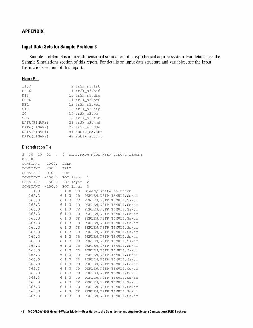
APPENDIX

Input Data Sets for Sample Problem 3

Sample problem 3 is a three-dimensional simulation of a hypothetical aquifer system. For details, see the Sample Simulations section of this report. For details on input data structure and variables, see the Input Instructions section of this report.

Name File

LIST 2 tr2k_s3.lstBAS6 1 tr2k_s3.ba6DIS 10 tr2k_s3.disBCF6 11 tr2k_s3.bc6WEL 12 tr2k_s3.welSIP 13 tr2k_s3.sipOC 15 tr2k_s3.ocSUB 19 tr2k_s3.subDATA(BINARY) 21 tr2k_s3.hedDATA(BINARY) 22 tr2k_s3.ddnDATA(BINARY) 41 sub1k_s3.sbsDATA(BINARY) 42 sub1k_s3.cmp

Discretization File

3 10 10 31 4 0 NLAY,NROW,NCOL,NPER,ITMUNI,LENUNI0 0 0CONSTANT 1000. DELRCONSTANT 2000. DELCCONSTANT 0.0 TOPCONSTANT -100.0 BOT layer 1CONSTANT -150.0 BOT layer 2CONSTANT -250.0 BOT layer 3 1.0 1 1.0 SS Steady state solution 365.3 6 1.3 TR PERLEN,NSTP,TSMULT,Ss/tr 365.3 6 1.3 TR PERLEN,NSTP,TSMULT,Ss/tr 365.3 6 1.3 TR PERLEN,NSTP,TSMULT,Ss/tr 365.3 6 1.3 TR PERLEN,NSTP,TSMULT,Ss/tr 365.3 6 1.3 TR PERLEN,NSTP,TSMULT,Ss/tr 365.3 6 1.3 TR PERLEN,NSTP,TSMULT,Ss/tr 365.3 6 1.3 TR PERLEN,NSTP,TSMULT,Ss/tr 365.3 6 1.3 TR PERLEN,NSTP,TSMULT,Ss/tr 365.3 6 1.3 TR PERLEN,NSTP,TSMULT,Ss/tr 365.3 6 1.3 TR PERLEN,NSTP,TSMULT,Ss/tr 365.3 6 1.3 TR PERLEN,NSTP,TSMULT,Ss/tr 365.3 6 1.3 TR PERLEN,NSTP,TSMULT,Ss/tr 365.3 6 1.3 TR PERLEN,NSTP,TSMULT,Ss/tr 365.3 6 1.3 TR PERLEN,NSTP,TSMULT,Ss/tr 365.3 6 1.3 TR PERLEN,NSTP,TSMULT,Ss/tr 365.3 6 1.3 TR PERLEN,NSTP,TSMULT,Ss/tr 365.3 6 1.3 TR PERLEN,NSTP,TSMULT,Ss/tr 365.3 6 1.3 TR PERLEN,NSTP,TSMULT,Ss/tr 365.3 6 1.3 TR PERLEN,NSTP,TSMULT,Ss/tr 365.3 6 1.3 TR PERLEN,NSTP,TSMULT,Ss/tr 365.3 6 1.3 TR PERLEN,NSTP,TSMULT,Ss/tr 365.3 6 1.3 TR PERLEN,NSTP,TSMULT,Ss/tr 365.3 6 1.3 TR PERLEN,NSTP,TSMULT,Ss/tr


365.3 6 1.3 TR PERLEN,NSTP,TSMULT,Ss/tr 365.3 6 1.3 TR PERLEN,NSTP,TSMULT,Ss/tr 365.3 6 1.3 TR PERLEN,NSTP,TSMULT,Ss/tr 365.3 6 1.3 TR PERLEN,NSTP,TSMULT,Ss/tr 365.3 6 1.3 TR PERLEN,NSTP,TSMULT,Ss/tr 365.3 6 1.3 TR PERLEN,NSTP,TSMULT,Ss/tr 365.3 6 1.3 TR PERLEN,NSTP,TSMULT,Ss/tr

Basic Package Input Data Set

#Sample Problem 3#SUB1 documentationNO OPTIONSINTERNAL 1 (20I4) 3 IBOUND layer 1 3 3 1 1 1 1 1 1 3 3 3 2 2 2 2 2 2 2 2 3 3 2 2 2 2 5 5 2 2 3 3 2 2 2 2 5 5 2 2 3 1 2 2 2 2 2 2 2 2 1 1 2 2 2 2 2 2 2 2 1 1 2 2 2 2 2 2 2 2 1 1 2 2 2 2 2 2 2 2 1 1 2 2 2 2 2 2 2 2 1 1 1 1 -4 -4 -4 -4 1 1 1CONSTANT 1 IBOUND layer 2CONSTANT 1 IBOUND layer 3 999.00 HNOFLOCONSTANT 0.0 0 Start Head, Layer 1CONSTANT 0.0 0 Start Head, Layer 2CONSTANT 0.0 0 Start Head, Layer 3

Block-Centered Flow Package Input Data Set

0 0.0 0 0.0 0 0 IBCFCB,HDRY,IWDFLG,WETFCT,IWETIT,IHDWET 1 0 0CONSTANT 1.0 TRPYCONSTANT 0.1 SF1 layer 1CONSTANT 20 HY layer 1CONSTANT 3.00E-06 VCONT layer 1CONSTANT 6.56E-05 SF1 layer 2INTERNAL 1.0 (10F7.0) 0 TRAN layer 2 1000. 1000. 1000. 1000. 1000. 1000. 1000. 1000. 1000. 1000. 1000. 0.5 0.5 0.5 0.5 0.5 0.5 0.5 0.5 1000. 1000. 0.5 0.5 0.5 0.5 0.5 0.5 0.5 0.5 1000. 1000. 0.5 0.5 0.5 0.5 0.5 0.5 0.5 0.5 1000. 1000. 0.5 0.5 0.5 0.5 0.5 0.5 0.5 0.5 1000. 1000. 0.5 0.5 0.5 0.5 0.5 0.5 0.5 0.5 1000. 1000. 0.5 0.5 0.5 0.5 0.5 0.5 0.5 0.5 1000. 1000. 0.5 0.5 0.5 0.5 0.5 0.5 0.5 0.5 1000. 1000. 0.5 0.5 0.5 0.5 0.5 0.5 0.5 0.5 1000. 1000. 1000. 1000. 1000. 1000. 1000. 1000. 1000. 1000. 1000.CONSTANT 3.00E-06 VCONT layer 2CONSTANT 2.62E-04 SF1 layer 3CONSTANT 1000. TRAN layer 3


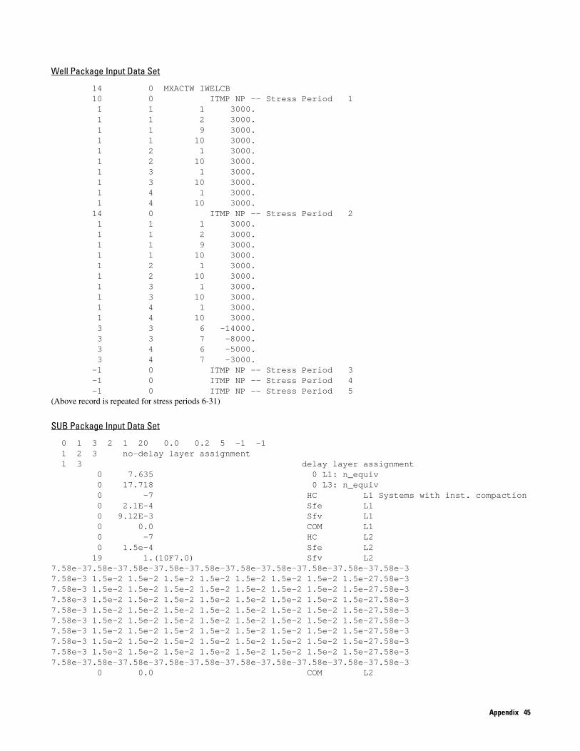
Well Package Input Data Set

14 0 MXACTW IWELCB 10 0 ITMP NP -- Stress Period 1 1 1 1 3000. 1 1 2 3000. 1 1 9 3000. 1 1 10 3000. 1 2 1 3000. 1 2 10 3000. 1 3 1 3000. 1 3 10 3000. 1 4 1 3000. 1 4 10 3000. 14 0 ITMP NP -- Stress Period 2 1 1 1 3000. 1 1 2 3000. 1 1 9 3000. 1 1 10 3000. 1 2 1 3000. 1 2 10 3000. 1 3 1 3000. 1 3 10 3000. 1 4 1 3000. 1 4 10 3000. 3 3 6 -14000. 3 3 7 -8000. 3 4 6 -5000. 3 4 7 -3000. -1 0 ITMP NP -- Stress Period 3 -1 0 ITMP NP -- Stress Period 4 -1 0 ITMP NP -- Stress Period 5(Above record is repeated for stress periods 6-31)

SUB Package Input Data Set

0 1 3 2 1 20 0.0 0.2 5 -1 -1 1 2 3 no-delay layer assignment 1 3 delay layer assignment 0 7.635 0 L1: n_equiv 0 17.718 0 L3: n_equiv 0 -7 HC L1 Systems with inst. compaction 0 2.1E-4 Sfe L1 0 9.12E-3 Sfv L1 0 0.0 COM L1 0 -7 HC L2 0 1.5e-4 Sfe L2 19 1.(10F7.0) Sfv L27.58e-37.58e-37.58e-37.58e-37.58e-37.58e-37.58e-37.58e-37.58e-37.58e-37.58e-3 1.5e-2 1.5e-2 1.5e-2 1.5e-2 1.5e-2 1.5e-2 1.5e-2 1.5e-27.58e-37.58e-3 1.5e-2 1.5e-2 1.5e-2 1.5e-2 1.5e-2 1.5e-2 1.5e-2 1.5e-27.58e-37.58e-3 1.5e-2 1.5e-2 1.5e-2 1.5e-2 1.5e-2 1.5e-2 1.5e-2 1.5e-27.58e-37.58e-3 1.5e-2 1.5e-2 1.5e-2 1.5e-2 1.5e-2 1.5e-2 1.5e-2 1.5e-27.58e-37.58e-3 1.5e-2 1.5e-2 1.5e-2 1.5e-2 1.5e-2 1.5e-2 1.5e-2 1.5e-27.58e-37.58e-3 1.5e-2 1.5e-2 1.5e-2 1.5e-2 1.5e-2 1.5e-2 1.5e-2 1.5e-27.58e-37.58e-3 1.5e-2 1.5e-2 1.5e-2 1.5e-2 1.5e-2 1.5e-2 1.5e-2 1.5e-27.58e-37.58e-3 1.5e-2 1.5e-2 1.5e-2 1.5e-2 1.5e-2 1.5e-2 1.5e-2 1.5e-27.58e-37.58e-37.58e-37.58e-37.58e-37.58e-37.58e-37.58e-37.58e-37.58e-37.58e-3 0 0.0 COM L2

Appendix 45

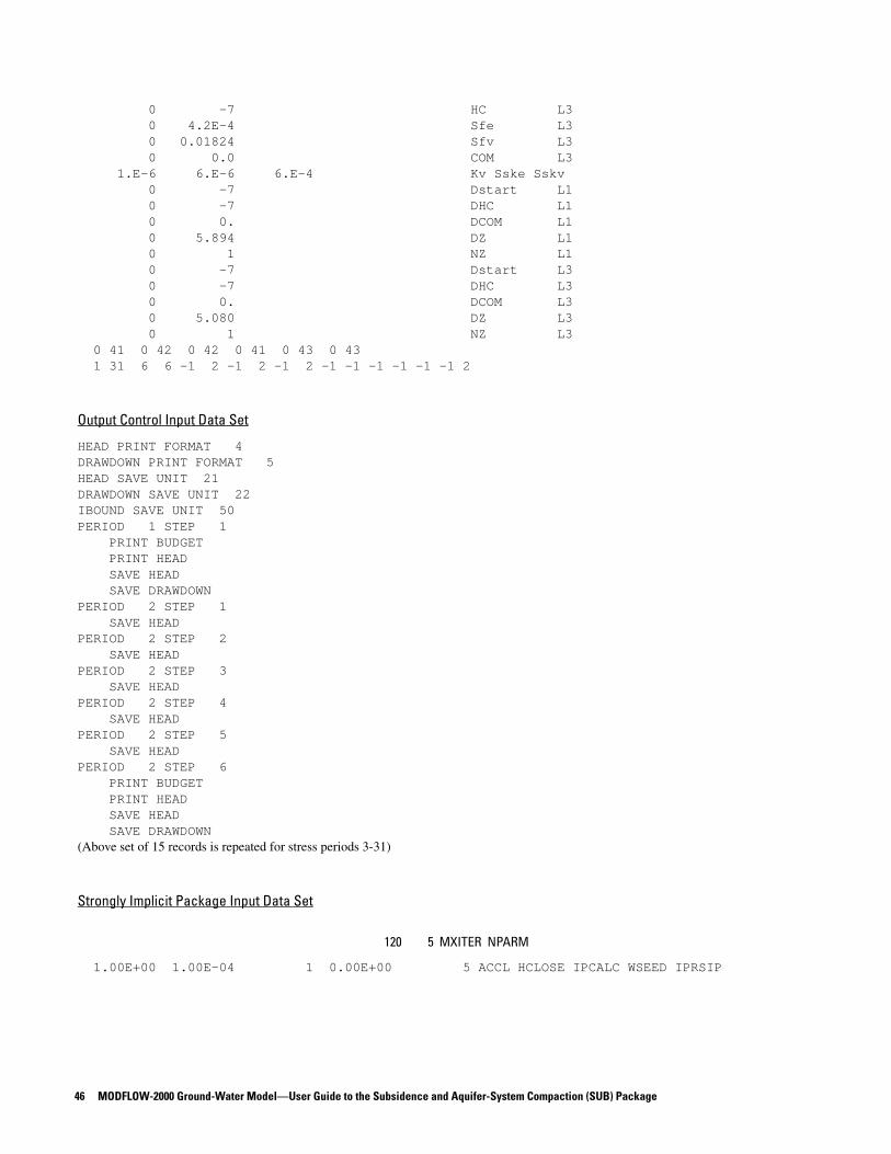
0 -7 HC L3 0 4.2E-4 Sfe L3 0 0.01824 Sfv L3 0 0.0 COM L3 1.E-6 6.E-6 6.E-4 Kv Sske Sskv 0 -7 Dstart L1 0 -7 DHC L1 0 0. DCOM L1 0 5.894 DZ L1 0 1 NZ L1 0 -7 Dstart L3 0 -7 DHC L3 0 0. DCOM L3 0 5.080 DZ L3 0 1 NZ L3 0 41 0 42 0 42 0 41 0 43 0 43 1 31 6 6 -1 2 -1 2 -1 2 -1 -1 -1 -1 -1 -1 2

Output Control Input Data Set

HEAD PRINT FORMAT 4DRAWDOWN PRINT FORMAT 5HEAD SAVE UNIT 21DRAWDOWN SAVE UNIT 22IBOUND SAVE UNIT 50PERIOD 1 STEP 1 PRINT BUDGET PRINT HEAD SAVE HEAD SAVE DRAWDOWNPERIOD 2 STEP 1 SAVE HEADPERIOD 2 STEP 2 SAVE HEADPERIOD 2 STEP 3 SAVE HEADPERIOD 2 STEP 4 SAVE HEADPERIOD 2 STEP 5 SAVE HEADPERIOD 2 STEP 6 PRINT BUDGET PRINT HEAD SAVE HEAD SAVE DRAWDOWN(Above set of 15 records is repeated for stress periods 3-31)

Strongly Implicit Package Input Data Set

120 5 MXITER NPARM

1.00E+00 1.00E-04 1 0.00E+00 5 ACCL HCLOSE IPCALC WSEED IPRSIP


Hoffmann, and others—

MODFLOW

-2000 GROUND-W

ATER MODEL—

USER GUIDE TO THE SUBSIDENCE AN

D AQUIFER-SYSTEM COM

PACTION (SUB) PACKAGE2—

U.S. Geological Survey Open-File Report 03—233

u.s. department of the interior u.s. geological … · u.s. department of the interior u.s....

Documents