U.S. EPA Benchmark DoseModeling GuidanceJ. Allen Davis, MSPH

National Center for Environmental Assessment, U.S. EPA

March 2, 2017

Brussels, Belgium

Disclaimer

The views expressed in this presentation are those of theauthor(s) and do not necessarily reflect the views orpolicies of the US EPA.

2

EPA’s BMD Technical Guidance

• Final version of the EPA’s Benchmark DoseTechnical Guidance document was publishedin 2012: https://www.epa.gov/risk/benchmark-dose-technical-guidance

• Other guidance documents relevant to BMDmodeling available at:http://epa.gov/iris/backgrd.html

• EPA’s Statistical Working Group periodicallyupdates recommended model practices

3

BMD Analysis Workflow

YesHave all models &model parametersbeen considered?

No

No

No

1. Choose BMR(s) and dose metrics to evaluate.

6. Document the BMD analysis, including uncertainties, as outlined in reporting requirements.

Consider combiningBMDs (or BMDLs)

5. Is one model better than the others considering best fitand least complexity (i.e., lowest AIC)?

2. Select the set of appropriate models, setparameter options, and run models

3. Do any models adequately fit the data?

4. Are the BMDLs for the adequate models sufficientlyclose?

Use BMD (or BMDL) from the model with the lowest AIC

START

No

Use lowest reasonableBMDL

Yes

Yes

Yes

Data notamenable for BMD

modeling

4

BMR Selection: DichotomousData

• An extra risk of 10% is recommended as a standard (not default) reportinglevel for dichotomous data.

• Customarily used because it is at or near the limit of sensitivity in most cancerbioassays and in non-cancer bioassays of comparable size

• In some situations, use of different BMRs is supported

• Biological considerations sometimes support different BMRs (5% for frankeffects, >10% for precursor effects)

• When a study has greater than usual sensitivity, a lower BMR can be used (5%for developmental studies)

• Results for a 10% BMR should always be shown for comparison when usingdifferent BMRs.

5

BMR Selection: Continuous Data

BMR Type BMR Calculation

Standard Deviation: BMR = mean0 ± (BMRF × SD0)

Relative Deviation: BMR = mean0 ± (BMRF × mean0)

Absolute Deviation: BMR = mean0 ± BMRF

Point: BMR = BMRF

Extra (Hill only):BMRup = mean0 + BMRF × (meanmax - mean0)

BMRdown = mean0 - BMRF × (mean0 - meanmin)

Where:

mean0 = Modeled mean response at control dose

SD0 = Modeled standard deviation at control dose

BMRF = BMR factor (user input used to define BMR)

meanmax = Maximum mean response in dataset

meanmin = Minimum mean response in dataset 6

BMR Selection: Continuous Data

• Preferred approach is to select a BMR that corresponds to a level changethat represents a minimal biologically significant response (i.e., 10%decrease in body weight)

• In the absence of a biological consideration, a BMR of a change in themean equal to one control standard deviation (1.0 SD) from the controlmean is recommended.

• In some situations, use of different BMRs is supported

• For more severe effects, a BMR of 0.5 SD can be used

• Results for a 1 SD BMR should always be shown for comparison when usingdifferent BMRs.

7

Selection of a Specific Model

BiologicalInterpretation

Examples:• Dichotomous:

• Saturable processes demonstrating Michaelis-Menten kinetics(Dichotomous Hill model)

• Two-stage clonal expansion model (cancer endpoints)• Continuous:

• Can use the Hill or Exponential models for receptor-mediatedresponses

Policy Decision

• U.S. EPA’s IRIS program uses the multistage model for cancer data (i.e.,dichotomous data)

• sufficiently flexible to fit most cancer bioassay data• provides consistency across cancer assessments

• U.S. EPA’s OPP group uses the Exponential models for modelingacetylcholinesterase inhibition data

OtherwiseHowever, in the absence of biological or policy-driven considerations, criteriafor final model selection are usually based on whether various modelsmathematically describe the data

8

Traditional Dichotomous Models

Modelname

Functional form# of

Parametersa

Low DoseLinearity

Model fits

Multistage 1+nYes, if β1 > 0No, if β1 = 0

All purpose

Logistic 2 Yes Simple; no background

Probit 2 Yes Simple; no background

Log-logistic 3 NoAll purpose; S-shape with plateauat 100%

Log-probit 3 NoAll purpose; plateau S-shape withplateau at 100%

Gamma 3 No All purpose

Weibull 3 No ”Hockey stick” shape

DichotomousHill

4 Yes Symmetrical, S-shape with plateau

a Background parameter = γ. Background for hill model = v × g

Modelname

Functional form# of

Parametersa

Low DoseLinearity

Model fits

Multistage 1+kYes, if β1 > 0No, if β1 = 0

All purpose

Logistic 2 Yes Simple; no background

Probit 2 Yes Simple; no background

Log-logistic 3 NoAll purpose; S-shape with plateauat 100%

Log-probit 3 NoAll purpose; plateau S-shape withplateau at 100%

Gamma 3 No All purpose

Weibull 3 No ”Hockey stick” shape

DichotomousHill

4 Yes Symmetrical, S-shape with plateau

a Background parameter = γ. Background for hill model = v × g

9

Continuous Model Forms

Model Name Functional Form # of Parameters Model Fits

Polynomiala 1 + nAll purpose, can fit non-symmetrical S-shaped datasetswith plateaus

Power 3 L-shaped

Hill 4Symmetrical, sigmoidal,S-shape with plateau

Exponentialb

Model 2Model 3Model 4Model 5

2334

All purpose (Models 2 & 3)Symmetrical andasymmetrical S-shape withplateau (Models 4 & 5)

a The stand-alone Linear model in BMDS is equal to a first-order polynomial modelb Nested family of 4 related models described by Slob (2002) and included in the PROAST software of RIVM

10

Restricting Model Parameters

• Model parameters (i.e., slope, background response, etc.) can be boundedto restrict the shape of the dose-response curve

• These restrictions can impact statistical calculations such as the goodness-of-fit p-value and AIC

• Currently, a parameter estimate that “hits a bound” impacts a model’s degreesof freedom (DF) (in BMDS, DF is increased by 1 for p-value calculation)

• When a parameter hits a bound, that parameter is not counted towards theAIC penalization (EPA’s Statistical Working Group may modify this approach inthe future)

• The use of model restrictions is a topic of ongoing discussion in EPA’sStatistical Working Group

11

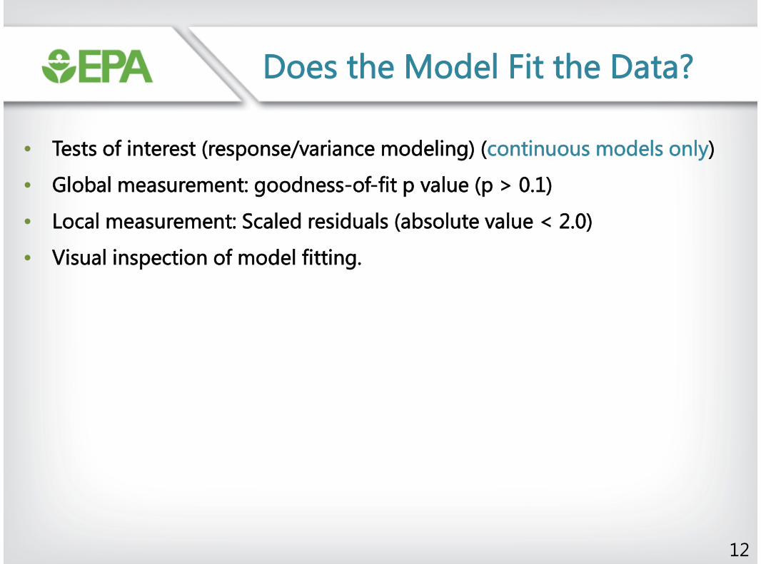
Does the Model Fit the Data?

• Tests of interest (response/variance modeling) (continuous models only)

• Global measurement: goodness-of-fit p value (p > 0.1)

• Local measurement: Scaled residuals (absolute value < 2.0)

• Visual inspection of model fitting.

12

Tests of Interest – Differences inResponses/Variances

• Test 1 – Do responses and/or variances differ among dose levels?

The p-value for Test 1 is less than .05.There appears to be adifference between response and/orvariances among the dose levels. Itseems appropriate to model the data

The p-value for Test 1 is greater than.05. There may not be adifference between responsesand/or variances among the doselevels. Modeling the data with adose/response curve may not beappropriate

13

1.58

1.6

1.62

1.64

1.66

1.68

1.7

1.72

1.74

0 50 100 150 200 250 300

Me

an

Re

sp

on

se

dose

Hill Model with 0.95 Confidence Level

11:10 03/04 2010

BMDBMDL

Hill

1.58

1.59

1.6

1.61

1.62

1.63

1.64

1.65

1.66

0 50 100 150 200 250 300

Me

an

Re

sp

on

se

dose11:18 03/04 2010

Linear

Tests of Interest – Variance

• In the current version BMDS, the distribution of continuous measures isassumed to be normal, with either a constant (homogenous) variance or avariance that changes as a power function of the mean value

• Var(i) = α[mean(i)]ρ

• ρ(rho) = 0, constant variance

• ρ(rho) ≠ 0, modeled variance

• Test 2 – Are variances homogenous?

• Test 3 – Are variances adequately modeled?

• Recommendation is to assume constant variance unless data clearlyindicate otherwise

14

Global Goodness-of-Fit

• BMDS provides a p-value to measure global goodness-of-fit

• Measures how model-predicted dose-group probability of responses differfrom the actual responses

• Small values indicate poor fit

• Recommended cut-off value is p = 0.10

• For models selected a priori due to biological or policy preferences (e.g.,multistage model for cancer endpoints), a cut-off value of p = 0.05 can beused

• What to do when goodness-of-fit is poor?

• Consider dropping high dose group(s) that negatively impact low dose fit

• Use PBPK model if available to calculate internal dose metrics that mayfacilitate better fit

• Log-transform doses if appropriate

15

Scaled Residuals

• Global goodness-of-fit p-values are not enough to assess local fit

• Models with large p-values may consistently “miss the data” (e.g., always onone side of the dose-group means)

• Models may “fit” the wrong (e.g. high-dose) region of the dose-responsecurve.

• Scaled Residuals – measure of how closely the model fits the data at eachpoint; 0 = exact fit

• Dichotomous data:� � � � � � �

√( � ∗ � ( � � � ))

• Continuous data:� � � � � � � � � � � � � � �

� � � � �

√ �

• Absolute values near the BMR should be lowest

• Question scaled residuals with absolute value > 2

16

Visual Inspection of Fit

17

0

0.1

0.2

0.3

0.4

0.5

0.6

0.7

0.8

0 50 100 150 200

Fra

ctio

nA

ffe

cte

d

dose

Multistage Model with 0.95 Confidence Level

22:08 06/25 2009

BMDBMDL

Multistage

0

0.1

0.2

0.3

0.4

0.5

0.6

0.7

0.8

0 50 100 150 200

Fra

ctio

nA

ffe

cte

d

dose

Multistage Model with 0.95 Confidence Level

22:05 06/25 2009

BMDBMDL

Multistage

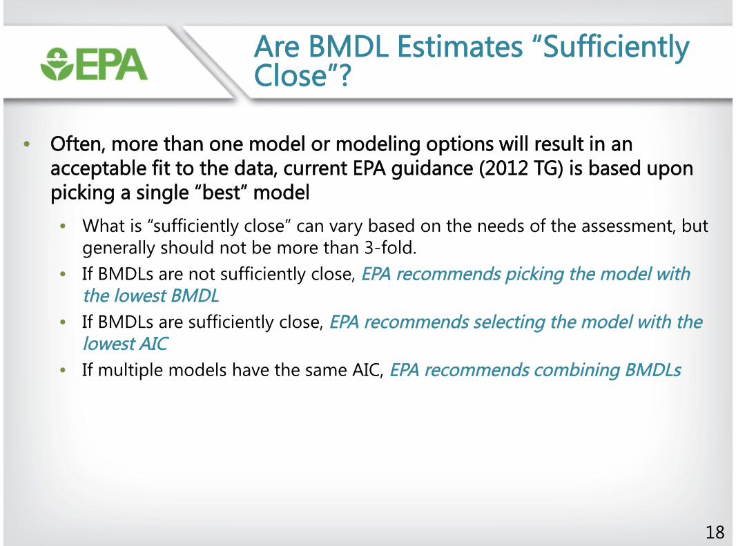
Are BMDL Estimates “SufficientlyClose”?

• Often, more than one model or modeling options will result in anacceptable fit to the data, current EPA guidance (2012 TG) is based uponpicking a single “best” model

• What is “sufficiently close” can vary based on the needs of the assessment, butgenerally should not be more than 3-fold.

• If BMDLs are not sufficiently close, EPA recommends picking the model withthe lowest BMDL

• If BMDLs are sufficiently close, EPA recommends selecting the model with thelowest AIC

• If multiple models have the same AIC, EPA recommends combining BMDLs

18

Example of BMD AnalysisDocumentation - Dichotomous

19

Example of BMD AnalysisDocumentation - Continuous

20

Example: EFSA DichotomousModel Selection

21

• All AIC > AICnull – 2(274.38)? No

• AICmin = 189.73

• AICmin > AICfull + 2(190.04)? No

• AICmin + 2 = 191.73

• Models with AIC ≤ AICmin + 2 = log-logisticand log-probit

• Lowest BMDL = 1.84(log-logistic)

• Largest BMDU = 5.11(log-probit)

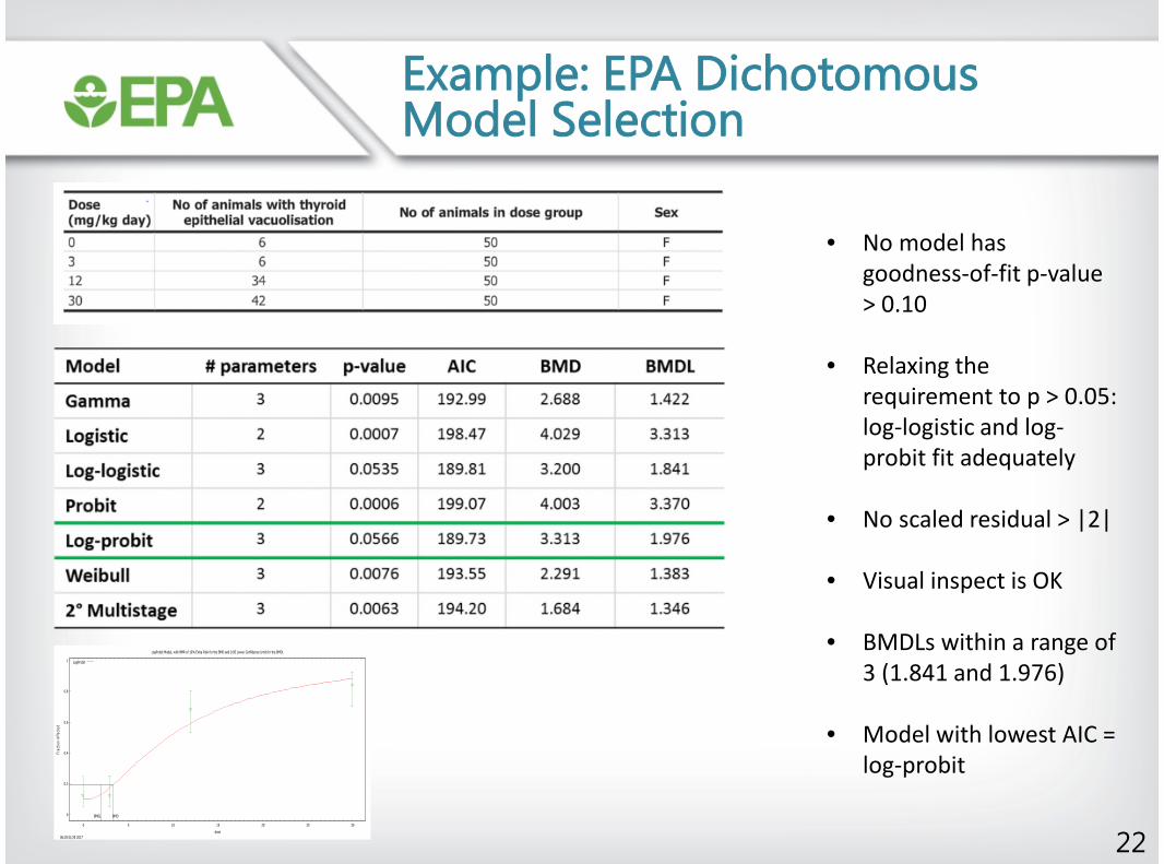
Example: EPA DichotomousModel Selection

22

• No model hasgoodness-of-fit p-value> 0.10

• Relaxing therequirement to p > 0.05:log-logistic and log-probit fit adequately

• No scaled residual > |2|

• Visual inspect is OK

• BMDLs within a range of3 (1.841 and 1.976)

• Model with lowest AIC =log-probit

0

0.2

0.4

0.6

0.8

1

0 5 10 15 20 25 30

Fra

ctio

nA

ffe

cte

d

dose

LogProbit Model, with BMR of 10% Extra Risk for the BMD and 0.95 Lower Confidence Limit for the BMDL

06:35 01/25 2017

BMDL BMD

LogProbit

Example: EFSA ContinuousModel Selection

23

• All AIC > AICnull – 2(-236.06)? No

• Model 3 for Exponentialand Hill models chosenbased on lowest AIC

• Lowest BMDL = 0.198(Exponential)

• Largest BMDU = 4.12(Hill)

Example: EPA Continuous ModelSelection

2434

36

38

40

42

44

0 0.2 0.4 0.6 0.8 1

Mean

Resp

onse

dose

Linear Model, with BMR of 0.1 Rel. Dev. for the BMD and 0.95 Lower Confidence Limit for the BMDL

06:59 01/25 2017

BMDBMDL

Linear

• All tests of fit (variance, global goodness-of-fit, and scaled residuals) indicate allmodels fit the data

• Exp5 and Hill model have no degrees offreedom to calculate p-value as # dosegroups = # estimated parameters

• Linear model selected due to lowest AIC(BMDLs for all models within a range of3)

• BMD = 0.247; BMDL = 0.226

• Compare to EFSA results: BMDL = 0.198

Updating EPA modelingprocedures

• EPA modifies its modeling procedures when necessary based on soundscience without updating formal technical guidance

• Updated modeling procedures & recommendations conveyed to the public viapublications, chemical assessments, or meeting presentations

• Examples include:

• A new analysis workflow for modeling cancer data with the multistage model

• Approximation methods to account for litter effects when only summarystatistics are available

• Use of AIC weights in model selection

• Use of historical controls

• Variance lack of fit

25

BMD Cancer Analysis Workflow

1. Choose BMR(s) and dose metrics to evaluate.

6. Document the BMD analysis, including uncertainties, as outlined in reporting requirements.

2. Fit all degrees of the multistage model (k-2groups) and run models

3. Are all parameter estimates positive (i.e., non-zero)?

START

Yes For models with appropriate fit, useBMD and BMDL from the model withthe lowest AIC

4. Fit 1st and 2nd degree model to the data and judgefit statistics (p-value, scaled residuals, visual fit)

5. Do both models fit adequately?

No

If any parameter is estimated to be zero, use the model withthe lowest BMDL. If not, use the model with the lowest AIC

If only one model fits adequately,use that model. If neither modelfits, consult statisticianYes

No

26

Modified Cancer Example

27

The β2 parameter for the 3° modelis estimated on the boundary

Therefore, only the 1° and 2°

models are considered further

Both models fit the dataadequately (p > 0.05, scaledresiduals < |2|)

As both models fit adequatelyAND no parameter for thesemodels is on a boundary, themodel with the lowest AIC ischosen

Therefore, the 1° model isselected using new workflow

3° model would’ve been chosenwith old workflow based on

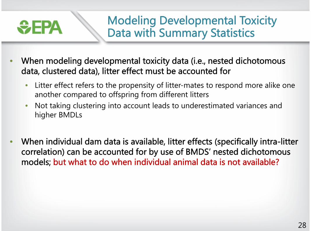
Modeling Developmental ToxicityData with Summary Statistics

• When modeling developmental toxicity data (i.e., nested dichotomousdata, clustered data), litter effect must be accounted for

• Litter effect refers to the propensity of litter-mates to respond more alike oneanother compared to offspring from different litters

• Not taking clustering into account leads to underestimated variances andhigher BMDLs

• When individual dam data is available, litter effects (specifically intra-littercorrelation) can be accounted for by use of BMDS’ nested dichotomousmodels; but what to do when individual animal data is not available?

28

Modeling Developmental ToxicityData with Summary Statistics

29

• Applying Rao-ScottTransformation (give avalue of ):

• Use dose-group totalsfor offspring: number ofoffspring ( � ), numberof affected fetuses ( � )

• Divide number ofoffspring ( � ) by

• Divide number ofaffected fetuses ( � ) by

• Rao-Scott transformeddata can now bemodeled with BMDSdichotomous models

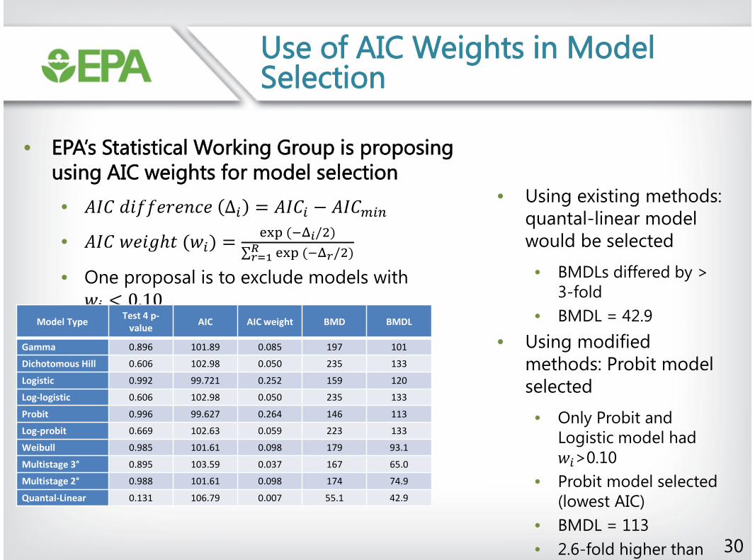
Use of AIC Weights in ModelSelection

• EPA’s Statistical Working Group is proposingusing AIC weights for model selection

• � � � � �

• �� � � ( � � � / � )

∑ � � � ( � � � / � )�� � �

• One proposal is to exclude models with

�

30

Model TypeTest 4 p-

valueAIC AIC weight BMD BMDL

Gamma 0.896 101.89 0.085 197 101

Dichotomous Hill 0.606 102.98 0.050 235 133

Logistic 0.992 99.721 0.252 159 120

Log-logistic 0.606 102.98 0.050 235 133

Probit 0.996 99.627 0.264 146 113

Log-probit 0.669 102.63 0.059 223 133

Weibull 0.985 101.61 0.098 179 93.1

Multistage 3° 0.895 103.59 0.037 167 65.0

Multistage 2° 0.988 101.61 0.098 174 74.9

Quantal-Linear 0.131 106.79 0.007 55.1 42.9

• Using existing methods:quantal-linear modelwould be selected

• BMDLs differed by >3-fold

• BMDL = 42.9

• Using modifiedmethods: Probit modelselected

• Only Probit andLogistic model had

� >0.10

• Probit model selected(lowest AIC)

• BMDL = 113

• 2.6-fold higher thanold method