u.s. neighborhood income inequality in the 2005-2009 … · u.s. department of commerce economics...

U.S. Department of CommerceEconomics and Statistics Administration

U.S. CENSUS BUREAU

U.S. Neighborhood Income Inequality in the 2005–2009 PeriodAmerican Community Survey Reports

By Daniel H. Weinberg

ACS-16

Issued October 2011

INTRODUCTION

Income inequality is one measure of soci-etal conditions. Some have argued that large (and recently increasing) income inequality is potentially harmful to social stability—letting “the rich get richer while the poor get poorer” is thought to be bad for the United States. Others have argued that income inequality is one of the engines that drives economic growth and innovation and taxing away the incomes of those at the top end of the income distribution can stifle creativity and lower the well-being of everyone. This paper will not take a position as to the benefits or costs of income inequality, or examine the changes in inequality over time at a local level, but rather it will examine the extent to which income inequality differs spatially inside the United States, focus-ing on small geographic areas.

Spatial income inequality is neither intrinsically bad nor good. One would not expect much income inequality in neigh-borhoods consisting of new high-priced houses. Nor would one expect much in neighborhoods consisting of low-rent private or public housing. Some would indeed argue sorting of households by income within a city or metropolitan area is natural as it is a rare neighborhood that has all kinds and prices of housing. On the other hand, others would say that diversity in incomes among neighbors can enhance the social environment. The idea that households will sort themselves into neighborhoods with a narrow distri-bution of income dates at least as early as Thurow (1971) if not indeed to Tiebout (1956).

Income sorting might have negative consequences for the poor. Wheeler (2008) notes “The movement of high-income individuals away from the poor, for example, may leave the poor with relatively few jobs (e.g., Kain 1968) or reduce the extent to which the rich con-fer positive spillovers on the poor (e.g., Wilson 1987 and Benabou 1996).” Watson (2009) argues that “Income sorting affects the distribution of role models, peers, and social networks” and that “the characteristics of one’s neighbors and peers in school affect outcomes.” But, as Hardman and Ioannides (2004) state, “For the vast majority of US households, neighbors’ incomes and other character-istics are the market-driven outcome of individual choices. Households’ tastes for housing space, quality and access to jobs and amenities, together with their incomes and assets, define demand for housing types and locations. Prices set in the housing market determine what hous-ing units and neighborhoods households can afford.” Among the implications, as Watson notes, is that “if residential choice is sensitive to the income distribu-tion, economic policies that moderate or amplify income inequality may shape the cities in which we live.”

This paper will start at the national level to give the overall context for the level of U.S. income inequality and drill down through states and large cities to neigh-borhoods—here defined as census tracts (designed by local officials and experts to be relatively homogenous and to have an average of roughly 1,500 housing units and 4,000 people). The data to do

2 U.S. Census Bureau

so became available in December 2010—when the first-ever income inequality estimates were released for neighborhoods from the American Community Survey (ACS).1 Those period estimates cover the years 2005 through 2009 and thus average together the final years of economic growth in the first decade of the 21st century with the first years of downturn.2

The ACS was designed as a replace-ment for the Census 2000 long form—the previous source of neighborhood characteristics such as median household income. As an annual survey of roughly 3 million addresses, it provides an annual portrait of the demographic, social, economic, and housing char-acteristics of small towns, neigh-borhoods, and population groups. As part of their data dissemination, the Census Bureau publishes esti-mates on the Internet for median household income and for the Gini index of household income inequal-ity (the Gini index ranges from 0.0, when all households have equal shares of income, to 1.0, when one household has all the income and the rest none).3

THE MEASURES OF INEQUALITY

The Gini measure is supplemented here by two additional measures of inequality calculated from the source data—the ratio of house-hold income at the 90th percentile to that at the 10th (called here the P90/10 index), and the ratio

1 Thus the census tracts boundaries are defined as of 2000, for use with that census. Data released in late 2011 from the ACS will use the 2010 Census tract boundaries.

2 Income is asked of respondents about the prior 12-month period, so interviews in January 2005 covered calendar year 2004 income, and interviews in December 2009 covered income for December 2008 through November 2009. The National Bureau of Economic Research dates the most recent recession as December 2007 to June 2009.

3 For more information on measurement of income in the ACS and on the Gini index of inequality, see Bishaw and Semega 2008.

of household income at the 95th percentile to that at the 20th (called here the P95/20 index). While the Gini index is available for all places and tracts (of sufficient size), the P90/10 and P95/20 indexes are not, as some areas have 10th and even 20th percentile incomes of $0. Nevertheless, it is hoped that the two ratio measures will provide a useful additional perspective.

Not all neighborhoods in the United States are included in this study, because many have too few house-holds in the sample to allow for the computation of reliable statistics. An admittedly arbitrary decision was made to exclude all census tracts (and places) with fewer than 50 interviews in the 5-year period under study from the tabulations presented below, though the com-putations for higher levels of geog-raphy include all households. All significance testing is performed at the 90 percent confidence level.

THE NATIONAL PICTURE

Each year, the Census Bureau publishes an estimate of national income inequality from the Current Population Survey Annual Social and Economic Supplement (CPS ASEC; the latest is DeNavas-Walt et al. 2010). According to analysis of that survey (which has been measuring income inequality since 1947) by Jones and Weinberg 2000 (see also Weinberg 1996), “between 1967 (when income data for households first became available) and 1992, the shape of the house-hold income distribution changed dramatically. This 25-year period was one of increasing household income inequality—as evidenced by several measures.” Subdividing that period, and using the Gini index as the measure, Jones and Weinberg observed that “household income inequality was generally stable between 1967 and 1980.” However,

they go on to note that “In contrast to the . . . Gini measures, . . . percentile measures . . . suggest that household income inequality increased from 1967 to 1980 . . . .The 95/20 ratio . . . increased from 1967 to 1980, while the 90/10 ratio . . . declined.” Despite the ambiguity in the 1967–1980 period, they conclude “it is clear that the household income distribution became increasingly unequal beginning in 1981.” Their study ended with 1998 data, but the Census Bureau statistics con-tinue to show increases in inequal-ity since then. The Gini coefficient for household income in 2009 was 0.468, higher than for 1998 (0.456).4

The basic CPS Gini measure of income inequality is now supple-mented with a parallel CPS mea-sure that attempts to correct for household size in computing the indexes, since households with more people tend to have more workers and therefore higher incomes. “Household Equivalent Income” (HEI) is computed by using the three-parameter equivalence scale used to compute the poverty thresholds used in the Census Bureau’s series of supplemental poverty measures. As expected, Gini indexes for HEI are typically lower (show more equality) than for unadjusted household income; indeed the HEI Gini indexes were all statistically lower than the unad-justed Ginis for each year over the 1977–2009 period (see DeNavas-Walt et al. 2010, Table A-3).5 The HEI Gini was lower in 1977 than in 2009 (0.369 versus 0.458, respec-tively) and like the unadjusted Gini the series of HEI Gini estimates

4 The Gini index for 1998 was lower than in 2001, 2004–2006, 2008, and 2009 and not statistically different from that in 1999, 2000, 2002, 2003, and 2007.

5 The earliest year for which the Gini index for HEI has been calculated is 1967; the full series was first published by the Census Bureau in DeNavas-Walt et al. (2010).

U.S. Census Bureau 3

demonstrates a growth in income inequality over the period. Because rankings based on the HEI Gini dif-fer little from those based on the (unadjusted) household income-based Gini, income inequality measures based on this alternative measure of income will not be pur-sued further in this paper.

The national P90/10 ratio based on data from the CPS ASEC stood at 11.36 in 2009, was not statistically different from the ratios for 2003, 2005, 2007, and 2008, but higher than for any other prior year (and up from 10.44 in 1998 and up from the lowest recorded since 1967—8.53 in 1975).6 The CPS ASEC P95/20 ratio stood at 8.80 in 2009, higher than for 2004 or any year prior to that (and up from 8.20 in 1998 and from the lowest recorded since 1967—5.97 in 1968).7

The Gini coefficient for household income as measured by the ACS rather than the CPS for 2009 was 0.469, not statistically different from the CPS measure. The Gini measures from the CPS and the ACS are compared in Table 1.8 Note that there is no reason to expect the statistics to agree exactly—the surveys are very different.9

6 The P90/10 for 1975 was not statisti-cally different from that ratio in 1968, 1974, 1976, or 1977.

7 The P95/20 for 1968 was not statisti-cally different from that ratio in 1969.

8 The CPS and ACS Gini estimates are not statistically different for 3 of the 5 years (2007 through 2009), but the CPS measure is higher in 2005 and 2006. The CPS Gini for 2010 was 0.469 (standard error of 0.0027), which was not statistically different from the ACS Gini for 2010 of 0.469 (standard error of 0.0006), or from any of the CPS Gini esti-mates from 2005 to 2009.

9 See “Guidance About Income Sources” at <www.census.gov/hhes/www/income /method/guidance/index.html> for guid-ance on using the income data from the two surveys. For example, “Each of these surveys differs from the others in some ways, such as the length and detail of its questionnaire, the number of households included (sample size), and the methodology used to collect and process the data . . . . The CPS ASEC is the preferred source for national analysis . . . . The ACS is preferred for subnational data on income.”

Table 2 shows the P90/10 and P95/20 income inequality mea-sures for the ACS. These ratios show basically the same time series story as did the Gini coefficient—an increase in income inequality from 2006 to 2009.10 Following the guidance from the Census Bureau income experts, ACS data will be used for subnational comparisons.

STATE AND MICROPOLITAN/METROPOLITAN AREA-LEVEL INCOME INEQUALITY

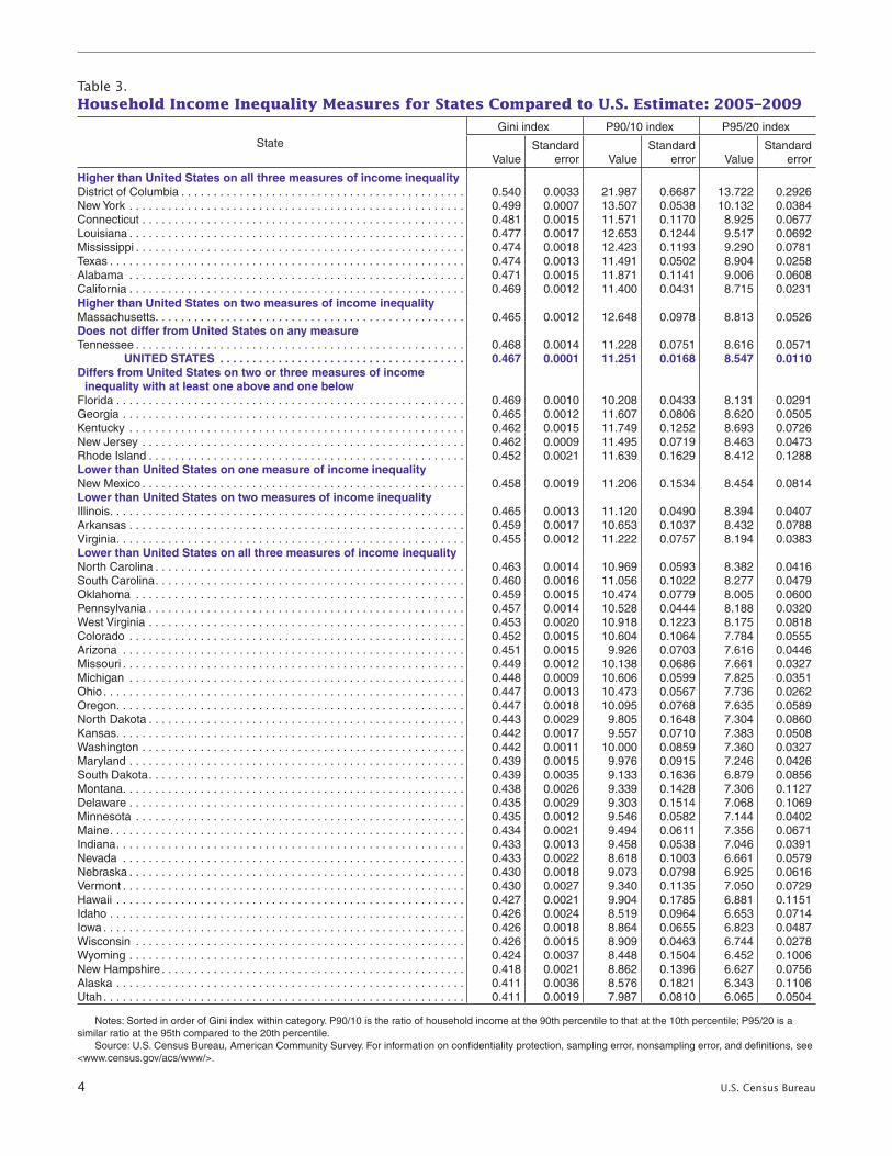
Table 3 presents the Gini, P90/10, and P95/20 measures of income

10 For the P90/10 ratio, neither of the changes from 2005 or 2006 to 2007 was sig-nificant. For the P95/20 ratio, the differences from 2005 to 2006 and 2007 to 2008 were not significant.

inequality for the United States as a whole and for the 50 states plus the District of Columbia for 2005–2009.11 These measures are close substitutes—the Pearson rank correlation coefficients are 0.930, 0.968, and 0.978 for the three measures taken two at a time. There are only eight states that had income inequality higher than for the United States as a whole on all

11 While the ACS samples size is large enough to provide reliable estimates for areas or groups of 65,000 population or more every year, the 5-year estimates are used exclu-sively hereafter to allow comparisons across geographic areas of all sizes. The Puerto Rico Community Survey is part of the ACS and provides similar estimates for that entity and its geographic components but is not dis-cussed here. Puerto Rico’s income inequality is typically about the same as the District of Columbia but higher than for any state.

Table 1. Comparison of Gini Household Income Inequality Measure Between the Current Population Survey (CPS) and the American Community Survey (ACS): 2005–2009

Year

Inequality measure

Gini-CPS Gini-ACS

Measure Standard error Measure Standard error

2009. . . . . . . . . . . . 0.468 0.0028 0.469 0.00202008. . . . . . . . . . . . 0.466 0.0027 0.469 0.00092007. . . . . . . . . . . . 0.463 0.0029 0.467 0.00012006. . . . . . . . . . . . 0.470 0.0029 0.464 0.00052005. . . . . . . . . . . . 0.469 0.0029 0.464 0.0005

Note: CPS and ACS estimates significantly different for 2005 and 2006 only.

Source: U.S. Census Bureau, Current Population Survey Annual Social and Economic Supplement and American Community Survey. For information on confidentiality protection, sampling error, nonsampling error, and definitions, see <www.census.gov/apsd/techdoc/cps/cpsmar10.pdf> for the CPS and <www.census.gov/acs/www/> for the ACS.

Table 2. American Community Survey P90/10 and P95/20 Household Income Inequality Measures: 2005–2009

Year

Inequality measure

P90/10 P95/20

Measure Standard error Measure Standard error

2009. . . . . . . . . . . . 11.452 0.030 8.714 0.0382008. . . . . . . . . . . . 11.380 0.029 8.603 0.0412007. . . . . . . . . . . . 11.111 0.038 8.542 0.0292006. . . . . . . . . . . . 11.065 0.057 8.425 0.0172005. . . . . . . . . . . . 11.198 0.049 8.406 0.034

Notes: P90/10 is the ratio of household income at the 90th percentile to that at the 10th percentile; P95/20 is a similar ratio at the 95th compared to the 20th percentile.

Source: U.S. Census Bureau, American Community Survey. For information on confidentiality protec-tion, sampling error, nonsampling error, and definitions, see <www.census.gov/acs/www/>.


Table 3. Household Income Inequality Measures for States Compared to U.S. Estimate: 2005–2009

Gini index P90/10 index P95/20 indexState Standard Standard Standard

Value error Value error Value error

Higher than United States on all three measures of income inequalityDistrict of Columbia . . . . . . . . . . . . . . . . . . . . . . . . . . . . . . . . . . . . . . . . . . . . 0.540 0.0033 21.987 0.6687 13.722 0.2926New York . . . . . . . . . . . . . . . . . . . . . . . . . . . . . . . . . . . . . . . . . . . . . . . . . . . . 0.499 0.0007 13.507 0.0538 10.132 0.0384Connecticut . . . . . . . . . . . . . . . . . . . . . . . . . . . . . . . . . . . . . . . . . . . . . . . . . . 0.481 0.0015 11.571 0.1170 8.925 0.0677Louisiana . . . . . . . . . . . . . . . . . . . . . . . . . . . . . . . . . . . . . . . . . . . . . . . . . . . . 0.477 0.0017 12.653 0.1244 9.517 0.0692Mississippi . . . . . . . . . . . . . . . . . . . . . . . . . . . . . . . . . . . . . . . . . . . . . . . . . . . 0.474 0.0018 12.423 0.1193 9.290 0.0781Texas . . . . . . . . . . . . . . . . . . . . . . . . . . . . . . . . . . . . . . . . . . . . . . . . . . . . . . . 0.474 0.0013 11.491 0.0502 8.904 0.0258Alabama . . . . . . . . . . . . . . . . . . . . . . . . . . . . . . . . . . . . . . . . . . . . . . . . . . . . 0.471 0.0015 11.871 0.1141 9.006 0.0608California . . . . . . . . . . . . . . . . . . . . . . . . . . . . . . . . . . . . . . . . . . . . . . . . . . . . 0.469 0.0012 11.400 0.0431 8.715 0.0231Higher than United States on two measures of income inequalityMassachusetts . . . . . . . . . . . . . . . . . . . . . . . . . . . . . . . . . . . . . . . . . . . . . . . . 0.465 0.0012 12.648 0.0978 8.813 0.0526Does not differ from United States on any measureTennessee . . . . . . . . . . . . . . . . . . . . . . . . . . . . . . . . . . . . . . . . . . . . . . . . . . . 0.468 0.0014 11.228 0.0751 8.616 0.0571 UNITED STATES . . . . . . . . . . . . . . . . . . . . . . . . . . . . . . . . . . . . . . 0 .467 0 .0001 11 .251 0 .0168 8 .547 0 .0110Differs from United States on two or three measures of income

inequality with at least one above and one belowFlorida . . . . . . . . . . . . . . . . . . . . . . . . . . . . . . . . . . . . . . . . . . . . . . . . . . . . . . 0.469 0.0010 10.208 0.0433 8.131 0.0291Georgia . . . . . . . . . . . . . . . . . . . . . . . . . . . . . . . . . . . . . . . . . . . . . . . . . . . . . 0.465 0.0012 11.607 0.0806 8.620 0.0505Kentucky . . . . . . . . . . . . . . . . . . . . . . . . . . . . . . . . . . . . . . . . . . . . . . . . . . . . 0.462 0.0015 11.749 0.1252 8.693 0.0726New Jersey . . . . . . . . . . . . . . . . . . . . . . . . . . . . . . . . . . . . . . . . . . . . . . . . . . 0.462 0.0009 11.495 0.0719 8.463 0.0473Rhode Island . . . . . . . . . . . . . . . . . . . . . . . . . . . . . . . . . . . . . . . . . . . . . . . . . 0.452 0.0021 11.639 0.1629 8.412 0.1288Lower than United States on one measure of income inequalityNew Mexico . . . . . . . . . . . . . . . . . . . . . . . . . . . . . . . . . . . . . . . . . . . . . . . . . . 0.458 0.0019 11.206 0.1534 8.454 0.0814Lower than United States on two measures of income inequalityIllinois . . . . . . . . . . . . . . . . . . . . . . . . . . . . . . . . . . . . . . . . . . . . . . . . . . . . . . . 0.465 0.0013 11.120 0.0490 8.394 0.0407Arkansas . . . . . . . . . . . . . . . . . . . . . . . . . . . . . . . . . . . . . . . . . . . . . . . . . . . . 0.459 0.0017 10.653 0.1037 8.432 0.0788Virginia . . . . . . . . . . . . . . . . . . . . . . . . . . . . . . . . . . . . . . . . . . . . . . . . . . . . . . 0.455 0.0012 11.222 0.0757 8.194 0.0383Lower than United States on all three measures of income inequalityNorth Carolina . . . . . . . . . . . . . . . . . . . . . . . . . . . . . . . . . . . . . . . . . . . . . . . . 0.463 0.0014 10.969 0.0593 8.382 0.0416South Carolina . . . . . . . . . . . . . . . . . . . . . . . . . . . . . . . . . . . . . . . . . . . . . . . . 0.460 0.0016 11.056 0.1022 8.277 0.0479Oklahoma . . . . . . . . . . . . . . . . . . . . . . . . . . . . . . . . . . . . . . . . . . . . . . . . . . . 0.459 0.0015 10.474 0.0779 8.005 0.0600Pennsylvania . . . . . . . . . . . . . . . . . . . . . . . . . . . . . . . . . . . . . . . . . . . . . . . . . 0.457 0.0014 10.528 0.0444 8.188 0.0320West Virginia . . . . . . . . . . . . . . . . . . . . . . . . . . . . . . . . . . . . . . . . . . . . . . . . . 0.453 0.0020 10.918 0.1223 8.175 0.0818Colorado . . . . . . . . . . . . . . . . . . . . . . . . . . . . . . . . . . . . . . . . . . . . . . . . . . . . 0.452 0.0015 10.604 0.1064 7.784 0.0555Arizona . . . . . . . . . . . . . . . . . . . . . . . . . . . . . . . . . . . . . . . . . . . . . . . . . . . . . 0.451 0.0015 9.926 0.0703 7.616 0.0446Missouri . . . . . . . . . . . . . . . . . . . . . . . . . . . . . . . . . . . . . . . . . . . . . . . . . . . . . 0.449 0.0012 10.138 0.0686 7.661 0.0327Michigan . . . . . . . . . . . . . . . . . . . . . . . . . . . . . . . . . . . . . . . . . . . . . . . . . . . . 0.448 0.0009 10.606 0.0599 7.825 0.0351Ohio . . . . . . . . . . . . . . . . . . . . . . . . . . . . . . . . . . . . . . . . . . . . . . . . . . . . . . . . 0.447 0.0013 10.473 0.0567 7.736 0.0262Oregon . . . . . . . . . . . . . . . . . . . . . . . . . . . . . . . . . . . . . . . . . . . . . . . . . . . . . . 0.447 0.0018 10.095 0.0768 7.635 0.0589North Dakota . . . . . . . . . . . . . . . . . . . . . . . . . . . . . . . . . . . . . . . . . . . . . . . . . 0.443 0.0029 9.805 0.1648 7.304 0.0860Kansas . . . . . . . . . . . . . . . . . . . . . . . . . . . . . . . . . . . . . . . . . . . . . . . . . . . . . . 0.442 0.0017 9.557 0.0710 7.383 0.0508Washington . . . . . . . . . . . . . . . . . . . . . . . . . . . . . . . . . . . . . . . . . . . . . . . . . . 0.442 0.0011 10.000 0.0859 7.360 0.0327Maryland . . . . . . . . . . . . . . . . . . . . . . . . . . . . . . . . . . . . . . . . . . . . . . . . . . . . 0.439 0.0015 9.976 0.0915 7.246 0.0426South Dakota . . . . . . . . . . . . . . . . . . . . . . . . . . . . . . . . . . . . . . . . . . . . . . . . . 0.439 0.0035 9.133 0.1636 6.879 0.0856Montana . . . . . . . . . . . . . . . . . . . . . . . . . . . . . . . . . . . . . . . . . . . . . . . . . . . . . 0.438 0.0026 9.339 0.1428 7.306 0.1127Delaware . . . . . . . . . . . . . . . . . . . . . . . . . . . . . . . . . . . . . . . . . . . . . . . . . . . . 0.435 0.0029 9.303 0.1514 7.068 0.1069Minnesota . . . . . . . . . . . . . . . . . . . . . . . . . . . . . . . . . . . . . . . . . . . . . . . . . . . 0.435 0.0012 9.546 0.0582 7.144 0.0402Maine . . . . . . . . . . . . . . . . . . . . . . . . . . . . . . . . . . . . . . . . . . . . . . . . . . . . . . . 0.434 0.0021 9.494 0.0611 7.356 0.0671Indiana . . . . . . . . . . . . . . . . . . . . . . . . . . . . . . . . . . . . . . . . . . . . . . . . . . . . . . 0.433 0.0013 9.458 0.0538 7.046 0.0391Nevada . . . . . . . . . . . . . . . . . . . . . . . . . . . . . . . . . . . . . . . . . . . . . . . . . . . . . 0.433 0.0022 8.618 0.1003 6.661 0.0579Nebraska . . . . . . . . . . . . . . . . . . . . . . . . . . . . . . . . . . . . . . . . . . . . . . . . . . . . 0.430 0.0018 9.073 0.0798 6.925 0.0616Vermont . . . . . . . . . . . . . . . . . . . . . . . . . . . . . . . . . . . . . . . . . . . . . . . . . . . . . 0.430 0.0027 9.340 0.1135 7.050 0.0729Hawaii . . . . . . . . . . . . . . . . . . . . . . . . . . . . . . . . . . . . . . . . . . . . . . . . . . . . . . 0.427 0.0021 9.904 0.1785 6.881 0.1151Idaho . . . . . . . . . . . . . . . . . . . . . . . . . . . . . . . . . . . . . . . . . . . . . . . . . . . . . . . 0.426 0.0024 8.519 0.0964 6.653 0.0714Iowa . . . . . . . . . . . . . . . . . . . . . . . . . . . . . . . . . . . . . . . . . . . . . . . . . . . . . . . . 0.426 0.0018 8.864 0.0655 6.823 0.0487Wisconsin . . . . . . . . . . . . . . . . . . . . . . . . . . . . . . . . . . . . . . . . . . . . . . . . . . . 0.426 0.0015 8.909 0.0463 6.744 0.0278Wyoming . . . . . . . . . . . . . . . . . . . . . . . . . . . . . . . . . . . . . . . . . . . . . . . . . . . . 0.424 0.0037 8.448 0.1504 6.452 0.1006New Hampshire . . . . . . . . . . . . . . . . . . . . . . . . . . . . . . . . . . . . . . . . . . . . . . . 0.418 0.0021 8.862 0.1396 6.627 0.0756Alaska . . . . . . . . . . . . . . . . . . . . . . . . . . . . . . . . . . . . . . . . . . . . . . . . . . . . . . 0.411 0.0036 8.576 0.1821 6.343 0.1106Utah . . . . . . . . . . . . . . . . . . . . . . . . . . . . . . . . . . . . . . . . . . . . . . . . . . . . . . . . 0.411 0.0019 7.987 0.0810 6.065 0.0504

Notes: Sorted in order of Gini index within category. P90/10 is the ratio of household income at the 90th percentile to that at the 10th percentile; P95/20 is a similar ratio at the 95th compared to the 20th percentile.

Source: U.S. Census Bureau, American Community Survey. For information on confidentiality protection, sampling error, nonsampling error, and definitions, see <www.census.gov/acs/www/>.


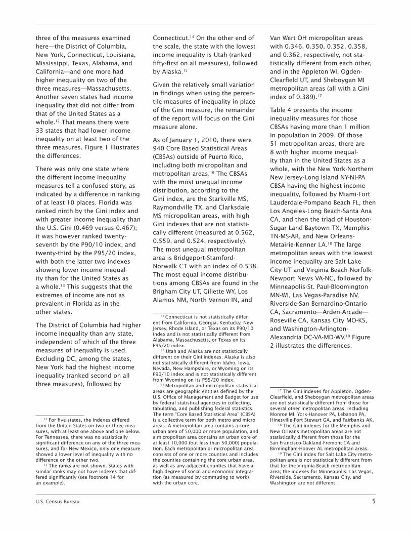
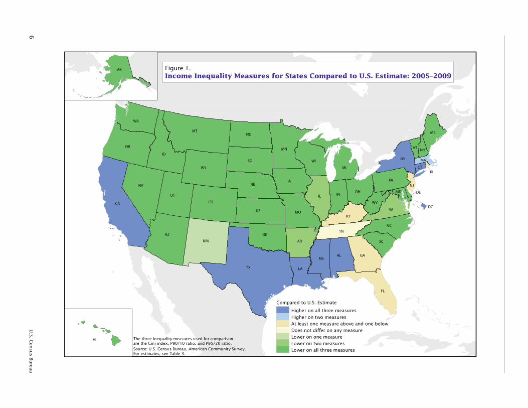
three of the measures examined here—the District of Columbia, New York, Connecticut, Louisiana, Mississippi, Texas, Alabama, and California—and one more had higher inequality on two of the three measures—Massachusetts. Another seven states had income inequality that did not differ from that of the United States as a whole.12 That means there were 33 states that had lower income inequality on at least two of the three measures. Figure 1 illustrates the differences.

There was only one state where the different income inequality measures tell a confused story, as indicated by a difference in ranking of at least 10 places. Florida was ranked ninth by the Gini index and with greater income inequality than the U.S. Gini (0.469 versus 0.467); it was however ranked twenty-seventh by the P90/10 index, and twenty-third by the P95/20 index, with both the latter two indexes showing lower income inequal-ity than for the United States as a whole.13 This suggests that the extremes of income are not as prevalent in Florida as in the other states.

The District of Columbia had higher income inequality than any state, independent of which of the three measures of inequality is used. Excluding DC, among the states, New York had the highest income inequality (ranked second on all three measures), followed by

12 For five states, the indexes differed from the United States on two or three mea-sures, with at least one above and one below. For Tennessee, there was no statistically significant difference on any of the three mea-sures, and for New Mexico, only one measure showed a lower level of inequality with no difference on the other two.

13 The ranks are not shown. States with similar ranks may not have indexes that dif-fered significantly (see footnote 14 for an example).

Connecticut.14 On the other end of the scale, the state with the lowest income inequality is Utah (ranked fifty-first on all measures), followed by Alaska.15

Given the relatively small variation in findings when using the percen-tile measures of inequality in place of the Gini measure, the remainder of the report will focus on the Gini measure alone.

As of January 1, 2010, there were 940 Core Based Statistical Areas (CBSAs) outside of Puerto Rico, including both micropolitan and metropolitan areas.16 The CBSAs with the most unequal income distribution, according to the Gini index, are the Starkville MS, Raymondville TX, and Clarksdale MS micropolitan areas, with high Gini indexes that are not statisti-cally different (measured at 0.562, 0.559, and 0.524, respectively). The most unequal metropolitan area is Bridgeport-Stamford-Norwalk CT with an index of 0.538. The most equal income distribu-tions among CBSAs are found in the Brigham City UT, Gillette WY, Los Alamos NM, North Vernon IN, and

14 Connecticut is not statistically differ-ent from California, Georgia, Kentucky, New Jersey, Rhode Island, or Texas on its P90/10 index and is not statistically different from Alabama, Massachusetts, or Texas on its P95/20 index.

15 Utah and Alaska are not statistically different on their Gini indexes. Alaska is also not statistically different from Idaho, Iowa, Nevada, New Hampshire, or Wyoming on its P90/10 index and is not statistically different from Wyoming on its P95/20 index.

16 Metropolitan and micropolitan statistical areas are geographic entities defined by the U.S. Office of Management and Budget for use by federal statistical agencies in collecting, tabulating, and publishing federal statistics. The term “Core Based Statistical Area” (CBSA) is a collective term for both metro and micro areas. A metropolitan area contains a core urban area of 50,000 or more population, and a micropolitan area contains an urban core of at least 10,000 (but less than 50,000) popula-tion. Each metropolitan or micropolitan area consists of one or more counties and includes the counties containing the core urban area, as well as any adjacent counties that have a high degree of social and economic integra-tion (as measured by commuting to work) with the urban core.

Van Wert OH micropolitan areas with 0.346, 0.350, 0.352, 0.358, and 0.362, respectively, not sta-tistically different from each other, and in the Appleton WI, Ogden-Clearfield UT, and Sheboygan MI metropolitan areas (all with a Gini index of 0.389).17

Table 4 presents the income inequality measures for those CBSAs having more than 1 million in population in 2009. Of those 51 metropolitan areas, there are 8 with higher income inequal-ity than in the United States as a whole, with the New York-Northern New Jersey-Long Island NY-NJ-PA CBSA having the highest income inequality, followed by Miami-Fort Lauderdale-Pompano Beach FL, then Los Angeles-Long Beach-Santa Ana CA, and then the triad of Houston-Sugar Land-Baytown TX, Memphis TN-MS-AR, and New Orleans-Metairie-Kenner LA.18 The large metropolitan areas with the lowest income inequality are Salt Lake City UT and Virginia Beach-Norfolk-Newport News VA-NC, followed by Minneapolis-St. Paul-Bloomington MN-WI, Las Vegas-Paradise NV, Riverside-San Bernardino-Ontario CA, Sacramento—Arden-Arcade—Roseville CA, Kansas City MO-KS, and Washington-Arlington-Alexandria DC-VA-MD-WV.19 Figure 2 illustrates the differences.

17 The Gini indexes for Appleton, Ogden-Clearfield, and Sheboygan metropolitan areas are not statistically different from those for several other metropolitan areas, including Monroe MI, York-Hanover PA, Lebanon PA, Hinesville-Fort Stewart GA, and Fairbanks AK.

18 The Gini indexes for the Memphis and New Orleans metropolitan areas are not statistically different from those for the San Francisco-Oakland-Fremont CA and Birmingham-Hoover AL metropolitan areas.

19 The Gini index for Salt Lake City metro-politan area is not statistically different from that for the Virginia Beach metropolitan area; the indexes for Minneapolis, Las Vegas, Riverside, Sacramento, Kansas City, and Washington are not different.

6

U.S. C

ensu

s Bureau

Source: U.S. Census Bureau, American Community Survey.For estimates, see Table 3.

Compared to U.S. Estimate

Higher on all three measuresHigher on two measuresAt least one measure above and one belowDoes not differ on any measureLower on one measureLower on two measuresLower on all three measures

The three inequality measures used for comparisonare the Gini index, P90/10 ratio, and P95/20 ratio.

AK

MDUT

NV

CA

MT

AZ

WY

TX

CO

NM

OK

KS

AR

NE

SD

IA

ND

MN

MO

LA

TN

MSGAAL

FL

SC

WI

KY

IL INOH

MI

VA

NC

WV

CT

PA

NY MA

ME

NJ

RI

WA

OR

ID

HI

VT NH

DE

DC

Figure 1.Income Inequality Measures for States Compared to U.S. Estimate: 2005–2009


Table 4. Gini Index of Household Income Inequality for Metropolitan Areas of Over 1 Million Population: 2005–2009

Metropolitan area Population Gini index Standard error

Higher income inequality than United StatesNew York-Northern New Jersey-Long Island, NY-NJ-PA . . . . . . . . . . . . . 18,912,644 0.502 0.0007Miami-Fort Lauderdale-Pompano Beach, FL. . . . . . . . . . . . . . . . . . . . . . 5,484,777 0.493 0.0015Los Angeles-Long Beach-Santa Ana, CA . . . . . . . . . . . . . . . . . . . . . . . . 12,762,126 0.484 0.0010Houston-Sugar Land-Baytown, TX . . . . . . . . . . . . . . . . . . . . . . . . . . . . . 5,595,262 0.478 0.0015Memphis, TN-MS-AR . . . . . . . . . . . . . . . . . . . . . . . . . . . . . . . . . . . . . . . . 1,287,231 0.478 0.0029New Orleans-Metairie-Kenner, LA . . . . . . . . . . . . . . . . . . . . . . . . . . . . . . 1,153,788 0.476 0.0027San Francisco-Oakland-Fremont, CA . . . . . . . . . . . . . . . . . . . . . . . . . . . 4,218,534 0.473 0.0014Birmingham-Hoover, AL . . . . . . . . . . . . . . . . . . . . . . . . . . . . . . . . . . . . . 1,112,213 0.472 0.0027Same income inequality as the United States UNITED STATES . . . . . . . . . . . . . . . . . . . . . . . . . . . . . . . . . . . 301,461,533 0 .467 0 .0006Chicago-Naperville-Joliet, IL-IN-WI . . . . . . . . . . . . . . . . . . . . . . . . . . . . . 9,461,816 0.466 0.0010Boston-Cambridge-Quincy, MA-NH . . . . . . . . . . . . . . . . . . . . . . . . . . . . . 4,513,934 0.465 0.0015Charlotte-Gastonia-Concord, NC-SC . . . . . . . . . . . . . . . . . . . . . . . . . . . 1,641,257 0.464 0.0049Oklahoma City, OK . . . . . . . . . . . . . . . . . . . . . . . . . . . . . . . . . . . . . . . . . 1,191,174 0.464 0.0046San Antonio, TX . . . . . . . . . . . . . . . . . . . . . . . . . . . . . . . . . . . . . . . . . . . . 1,979,686 0.463 0.0041Lower income inequality than United StatesPhiladelphia-Camden-Wilmington, PA-NJ-DE-MD . . . . . . . . . . . . . . . . . 5,910,593 0.464 0.0021Cleveland-Elyria-Mentor, OH . . . . . . . . . . . . . . . . . . . . . . . . . . . . . . . . . . 2,101,821 0.462 0.0049Dallas-Fort Worth-Arlington, TX . . . . . . . . . . . . . . . . . . . . . . . . . . . . . . . . 6,144,234 0.461 0.0046Nashville-Davidson—Murfreesboro—Franklin, TN . . . . . . . . . . . . . . . . . 1,520,649 0.460 0.0041Tampa-St. Petersburg-Clearwater, FL . . . . . . . . . . . . . . . . . . . . . . . . . . . 2,702,390 0.459 0.0039Pittsburgh, PA . . . . . . . . . . . . . . . . . . . . . . . . . . . . . . . . . . . . . . . . . . . . . 2,360,259 0.459 0.0026Detroit-Warren-Livonia, MI . . . . . . . . . . . . . . . . . . . . . . . . . . . . . . . . . . . . 4,452,548 0.454 0.0037Austin-Round Rock, TX . . . . . . . . . . . . . . . . . . . . . . . . . . . . . . . . . . . . . . 1,589,393 0.453 0.0038Buffalo-Niagara Falls, NY . . . . . . . . . . . . . . . . . . . . . . . . . . . . . . . . . . . . 1,128,813 0.453 0.0029Atlanta-Sandy Springs-Marietta, GA . . . . . . . . . . . . . . . . . . . . . . . . . . . . 5,238,994 0.452 0.0024San Diego-Carlsbad-San Marcos, CA . . . . . . . . . . . . . . . . . . . . . . . . . . . 2,987,543 0.451 0.0041Denver-Aurora-Broomfield, CO . . . . . . . . . . . . . . . . . . . . . . . . . . . . . . . . 2,451,038 0.450 0.0045St. Louis, MO-IL . . . . . . . . . . . . . . . . . . . . . . . . . . . . . . . . . . . . . . . . . . . . 2,803,776 0.448 0.0023San Jose-Sunnyvale-Santa Clara, CA . . . . . . . . . . . . . . . . . . . . . . . . . . . 1,784,130 0.448 0.0032Milwaukee-Waukesha-West Allis, WI . . . . . . . . . . . . . . . . . . . . . . . . . . . . 1,546,312 0.448 0.0031Phoenix-Mesa-Scottsdale, AZ . . . . . . . . . . . . . . . . . . . . . . . . . . . . . . . . . 4,151,634 0.447 0.0027Cincinnati-Middletown, OH-KY-IN . . . . . . . . . . . . . . . . . . . . . . . . . . . . . . 2,140,796 0.447 0.0029Indianapolis-Carmel, IN . . . . . . . . . . . . . . . . . . . . . . . . . . . . . . . . . . . . . . 1,695,807 0.447 0.0040Providence-New Bedford-Fall River, RI-MA . . . . . . . . . . . . . . . . . . . . . . . 1,602,591 0.447 0.0022Louisville-Jefferson County, KY-IN . . . . . . . . . . . . . . . . . . . . . . . . . . . . . . 1,235,476 0.447 0.0032Jacksonville, FL . . . . . . . . . . . . . . . . . . . . . . . . . . . . . . . . . . . . . . . . . . . . 1,294,684 0.446 0.0047Baltimore-Towson, MD . . . . . . . . . . . . . . . . . . . . . . . . . . . . . . . . . . . . . . 2,669,987 0.445 0.0029Columbus, OH . . . . . . . . . . . . . . . . . . . . . . . . . . . . . . . . . . . . . . . . . . . . . 1,758,531 0.445 0.0036Hartford-West Hartford-East Hartford, CT . . . . . . . . . . . . . . . . . . . . . . . . 1,186,939 0.443 0.0051Orlando-Kissimmee, FL . . . . . . . . . . . . . . . . . . . . . . . . . . . . . . . . . . . . . . 2,023,605 0.442 0.0029Seattle-Tacoma-Bellevue, WA . . . . . . . . . . . . . . . . . . . . . . . . . . . . . . . . . 3,306,836 0.440 0.0037Portland-Vancouver-Beaverton, OR-WA . . . . . . . . . . . . . . . . . . . . . . . . . 2,163,436 0.440 0.0031Richmond, VA . . . . . . . . . . . . . . . . . . . . . . . . . . . . . . . . . . . . . . . . . . . . . 1,209,484 0.437 0.0038Raleigh-Cary, NC . . . . . . . . . . . . . . . . . . . . . . . . . . . . . . . . . . . . . . . . . . . 1,042,848 0.437 0.0027Rochester, NY . . . . . . . . . . . . . . . . . . . . . . . . . . . . . . . . . . . . . . . . . . . . . 1,033,026 0.436 0.0036Washington-Arlington-Alexandria, DC-VA-MD-WV . . . . . . . . . . . . . . . . . 5,332,297 0.433 0.0043Kansas City, MO-KS . . . . . . . . . . . . . . . . . . . . . . . . . . . . . . . . . . . . . . . . 2,013,797 0.433 0.0042Sacramento—Arden-Arcade—Roseville, CA . . . . . . . . . . . . . . . . . . . . . 2,076,579 0.432 0.0043Riverside-San Bernardino-Ontario, CA . . . . . . . . . . . . . . . . . . . . . . . . . . 4,022,939 0.431 0.0021Las Vegas-Paradise, NV . . . . . . . . . . . . . . . . . . . . . . . . . . . . . . . . . . . . . 1,821,507 0.431 0.0030Minneapolis-St. Paul-Bloomington, MN-WI . . . . . . . . . . . . . . . . . . . . . . . 3,202,412 0.430 0.0031Virginia Beach-Norfolk-Newport News, VA-NC . . . . . . . . . . . . . . . . . . . . 1,669,614 0.421 0.0028Salt Lake City, UT . . . . . . . . . . . . . . . . . . . . . . . . . . . . . . . . . . . . . . . . . . 1,090,416 0.417 0.0042


8

U.S. C

ensu

s Bureau

Source: U.S. Census Bureau, American Community Survey.For estimates, see Table 4.

Higher Gini index than U.S. estimateSame Gini index as U.S. estimateLower Gini index than U.S. estimate

Figure 2.Gini Index for Metropolitan Areas With Population Over One Million Compared to U.S. Estimate: 2005–2009


COMPARING PLACES20

The Census Bureau definition of place is “A concentration of popula-tion either legally bounded as an incorporated place, or identified as a Census Designated Place (CDP). . . . Incorporated places have legal descriptions of borough (except in Alaska and New York), city, town (except in New England, New York, and Wisconsin), or village.” It is dif-ficult to identify the places with the highest and lowest levels of income inequality, as small areas have large sampling variability. Of the 17,823 places with at least 50 interviewed housing units in the sample, the 48 places with the highest measured Gini index and the 46 places with the lowest measured Gini index are all under 10,000 people.

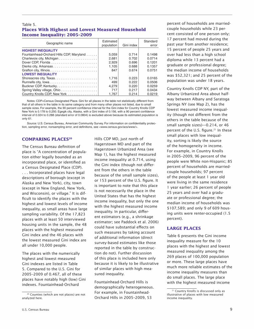
The places with the numerically highest and lowest measured Gini indexes are listed in Table 5. Compared to the U.S. Gini for 2005–2009 of 0.467, all of these places have notably high (low) Gini indexes. Fountainhead-Orchard

20 Counties (which are not places) are not analyzed here.

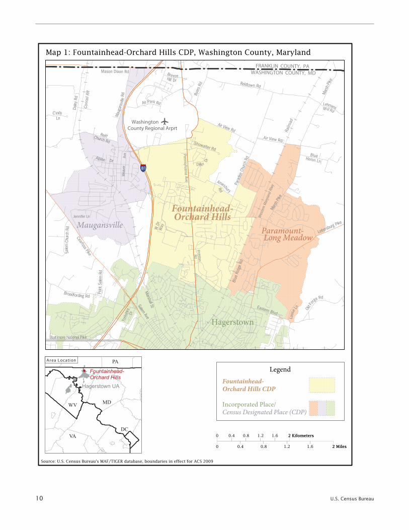
Hills CDP MD, just north of Hagerstown MD and part of the Hagerstown Urbanized Area (see Map 1), has the highest measured income inequality at 0.714, using the Gini index (though not differ-ent from the others in the table because of the small sample sizes), or 153 percent of the U.S. figure. It is important to note that this place is not necessarily the place in the United States that has the highest income inequality, but only the one with the highest measured income inequality. In particular, differ-ent estimators (e.g., a shrinkage estimator; see Paddock et al. 2006) could have substantial effects on such measures by taking account of additional information (direct survey-based estimates like those reported in the table by construc-tion do not). Further discussion of this place is included here only because it is likely to be illustrative of similar places with high mea-sured inequality.

Fountainhead-Orchard Hills is demographically heterogeneous. For example, in Fountainhead-Orchard Hills in 2005–2009, 53

percent of households are married-couple households while 23 per-cent consisted of one person only; 17 percent had moved during the past year from another residence; 15 percent of people 25 years and over had less than a high school diploma while 13 percent had a graduate or professional degree; the median income of households was $52,321; and 25 percent of the population was under 18 years.

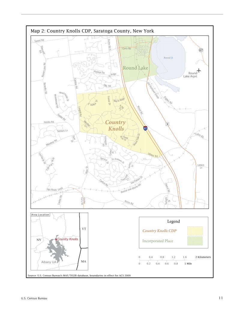
Country Knolls CDP NY, part of the Albany Urbanized Area about half-way between Albany and Saratoga Springs NY (see Map 2), has the lowest measured income inequal-ity (though not different from the others in the table because of the small sample sizes)—0.214, or 46 percent of the U.S. figure.21 In these small places with low inequal-ity, sorting is likely the source of the homogeneity in income. For example, in Country Knolls in 2005–2009, 96 percent of the people were White non-Hispanic; 85 percent of households are married-couple households; 97 percent of the people at least 1 year old were living in the same residence 1 year earlier; 26 percent of people 25 years and over had a gradu-ate or professional degree; the median income of households was $107,589; and only 9 of 609 hous-ing units were renter-occupied (1.5 percent).

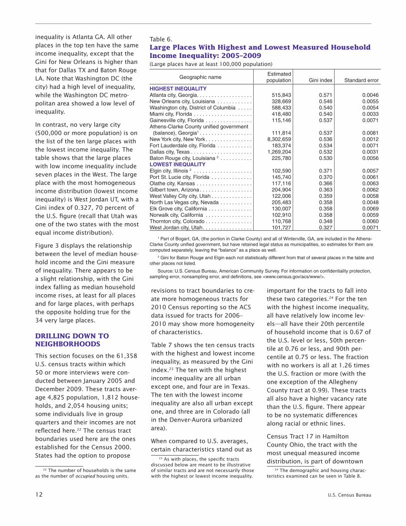
LARGE PLACES

Table 6 presents the Gini income inequality measure for the 10 places with the highest and lowest measured inequality among the 269 places of 100,000 population or more. These large places have much more reliable estimates of the income inequality measures than do small places. The large place with the highest measured income

21 Country Knolls is discussed only as illustrative of places with low measured income inequality.

Table 5. Places With Highest and Lowest Measured Household Income Inequality: 2005–2009

Geographic nameEstimated population Gini index

Standard error

HIGHEST INEQUALITY Fountainhead-Orchard Hills CDP, Maryland . . . . . . 5,059 0.714 0.1498Charlevoix city, Michigan . . . . . . . . . . . . . . . . . . . . . 2,681 0.702 0.0714Dover CDP, Florida . . . . . . . . . . . . . . . . . . . . . . . . . 2,929 0.696 0.1201Dierks city, Arkansas . . . . . . . . . . . . . . . . . . . . . . . . 1,105 0.688 0.1357Grafton city, Illinois . . . . . . . . . . . . . . . . . . . . . . . . . . 847 0.674 0.0751LOWEST INEQUALITY Shoreacres city, Texas . . . . . . . . . . . . . . . . . . . . . . . 1,716 0.223 0.0165Runnells city, Iowa . . . . . . . . . . . . . . . . . . . . . . . . . . 499 0.222 0.0506Buckner CDP, Kentucky . . . . . . . . . . . . . . . . . . . . . . 4,279 0.220 0.0259Spring Valley village, Ohio . . . . . . . . . . . . . . . . . . . . 717 0.217 0.0434Country Knolls CDP, New York . . . . . . . . . . . . . . . . 1,767 0.214 0.0219

Notes: CDP=Census Designated Place. Gini for all places in the table not statistically different from that of all others in the table in its same category and from many other places not listed, due to small sample sizes. For example, the 90 percent confidence interval for the Gini index for Country Knolls CDP New York is 0.178 to 0.250. Egegik city, Alaska, with a Gini index of 0.156, with a 90 percent confidence interval of 0.024 to 0.288 (standard error of 0.0804) is excluded above because its estimated population is only 61.

Source: U.S. Census Bureau, American Community Survey. For information on confidentiality protec-tion, sampling error, nonsampling error, and definitions, see <www.census.gov/acs/www/>.


PA

Hagerstown UA

VA

WV MD

DC

Fountainhead-Orchard Hills

Ar ea Locati on


NY

Albany UA

VT

MA

Country Knolls

Ar ea Locati on


inequality is Atlanta GA. All other places in the top ten have the same income inequality, except that the Gini for New Orleans is higher than that for Dallas TX and Baton Rouge LA. Note that Washington DC (the city) had a high level of inequality, while the Washington DC metro-politan area showed a low level of inequality.

In contrast, no very large city (500,000 or more population) is on the list of the ten large places with the lowest income inequality. The table shows that the large places with low income inequality include seven places in the West. The large place with the most homogeneous income distribution (lowest income inequality) is West Jordan UT, with a Gini index of 0.327, 70 percent of the U.S. figure (recall that Utah was one of the two states with the most equal income distribution).

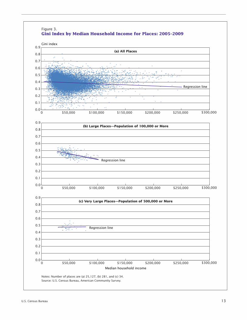
Figure 3 displays the relationship between the level of median house-hold income and the Gini measure of inequality. There appears to be a slight relationship, with the Gini index falling as median household income rises, at least for all places and for large places, with perhaps the opposite holding true for the 34 very large places.

DRILLING DOWN TO NEIGHBORHOODS

This section focuses on the 61,358 U.S. census tracts within which 50 or more interviews were con-ducted between January 2005 and December 2009. These tracts aver-age 4,825 population, 1,812 house-holds, and 2,054 housing units; some individuals live in group quarters and their incomes are not reflected here.22 The census tract boundaries used here are the ones established for the Census 2000. States had the option to propose

22 The number of households is the same as the number of occupied housing units.

revisions to tract boundaries to cre-ate more homogeneous tracts for 2010 Census reporting so the ACS data issued for tracts for 2006–2010 may show more homogeneity of characteristics.

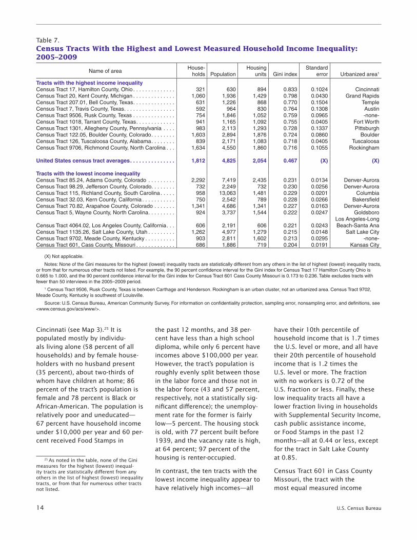
Table 7 shows the ten census tracts with the highest and lowest income inequality, as measured by the Gini index.23 The ten with the highest income inequality are all urban except one, and four are in Texas. The ten with the lowest income inequality are also all urban except one, and three are in Colorado (all in the Denver-Aurora urbanized area).

When compared to U.S. averages, certain characteristics stand out as

23 As with places, the specific tracts discussed below are meant to be illustrative of similar tracts and are not necessarily those with the highest or lowest income inequality.

important for the tracts to fall into these two categories.24 For the ten with the highest income inequality, all have relatively low income lev-els—all have their 20th percentile of household income that is 0.67 of the U.S. level or less, 50th percen-tile at 0.76 or less, and 90th per-centile at 0.75 or less. The fraction with no workers is all at 1.26 times the U.S. fraction or more (with the one exception of the Allegheny County tract at 0.99). These tracts all also have a higher vacancy rate than the U.S. figure. There appear to be no systematic differences along racial or ethnic lines.

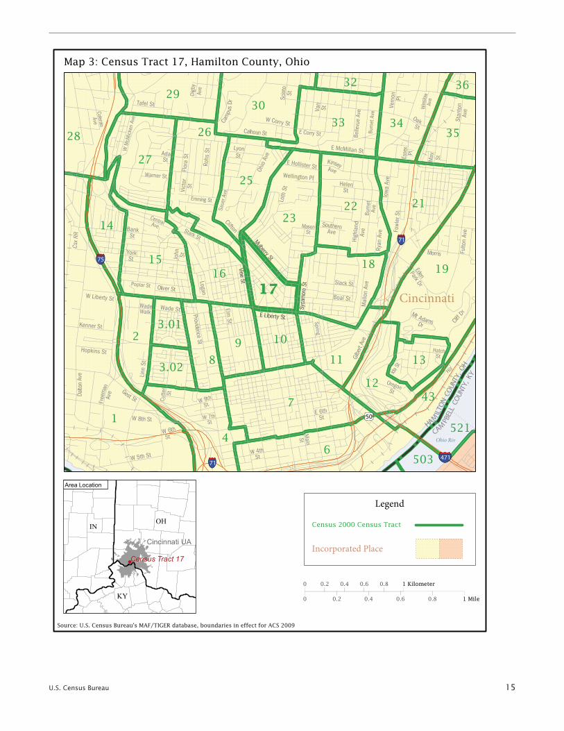
Census Tract 17 in Hamilton County Ohio, the tract with the most unequal measured income distribution, is part of downtown

24 The demographic and housing charac-teristics examined can be seen in Table 8.

Table 6. Large Places With Highest and Lowest Measured Household Income Inequality: 2005–2009(Large places have at least 100,000 population)

Geographic nameEstimated population Gini index Standard error

HIGHEST INEQUALITYAtlanta city, Georgia. . . . . . . . . . . . . . . . . . . 515,843 0.571 0.0046New Orleans city, Louisiana . . . . . . . . . . . . 328,669 0.546 0.0055Washington city, District of Columbia . . . . . 588,433 0.540 0.0054Miami city, Florida . . . . . . . . . . . . . . . . . . . . 418,480 0.540 0.0033Gainesville city, Florida . . . . . . . . . . . . . . . . 115,146 0.537 0.0071Athens-Clarke County unified government

(balance), Georgia1 . . . . . . . . . . . . . . . . . . 111,814 0.537 0.0081New York city, New York . . . . . . . . . . . . . . . . 8,302,659 0.536 0.0012Fort Lauderdale city, Florida . . . . . . . . . . . . 183,374 0.534 0.0071Dallas city, Texas . . . . . . . . . . . . . . . . . . . . . 1,269,204 0.532 0.0031Baton Rouge city, Louisiana 2 . . . . . . . . . . . 225,780 0.530 0.0056LOWEST INEQUALITYElgin city, Illinois 2 . . . . . . . . . . . . . . . . . . . . 102,590 0.371 0.0057Port St. Lucie city, Florida . . . . . . . . . . . . . . 145,740 0.370 0.0061Olathe city, Kansas . . . . . . . . . . . . . . . . . . . 117,116 0.366 0.0063Gilbert town, Arizona . . . . . . . . . . . . . . . . . . 204,904 0.363 0.0062West Valley City city, Utah . . . . . . . . . . . . . . 122,006 0.359 0.0058North Las Vegas city, Nevada . . . . . . . . . . . 205,483 0.358 0.0048Elk Grove city, California . . . . . . . . . . . . . . . 130,007 0.358 0.0069Norwalk city, California . . . . . . . . . . . . . . . . 102,910 0.358 0.0059Thornton city, Colorado . . . . . . . . . . . . . . . . 110,768 0.348 0.0060West Jordan city, Utah . . . . . . . . . . . . . . . . . 101,727 0.327 0.0071

1 Part of Bogart, GA, (the portion in Clarke County) and all of Winterville, GA, are included in the Athens-Clarke County unified government, but have retained legal status as municipalities, so estimates for them are computed separately, leaving the “balance” as a place as well.

2 Gini for Baton Rouge and Elgin each not statistically different from that of several places in the table and other places not listed.



Regression line

Regression line

Regression line

Gini index

Median household income

Figure 3.Gini Index by Median Household Income for Places: 2005–2009

Notes: Number of places are (a) 25,127, (b) 281, and (c) 34. Source: U.S. Census Bureau, American Community Survey.

0 $50,000 $100,000 $150,000 $200,000 $250,000 $300,0000.0

0.1

0.2

0.3

0.4

0.5

0.6

0.7

0.8

0.9(a) All Places

0 $50,000 $100,000 $150,000 $200,000 $250,000 $300,0000.0

0.1

0.2

0.3

0.4

0.5

0.6

0.7

0.8

0.9(b) Large Places—Population of 100,000 or More

0 $50,000 $100,000 $150,000 $200,000 $250,000 $300,0000.0

0.1

0.2

0.3

0.4

0.5

0.6

0.7

0.8

0.9(c) Very Large Places—Population of 500,000 or More


Cincinnati (see Map 3).25 It is populated mostly by individu-als living alone (58 percent of all households) and by female house-holders with no husband present (35 percent), about two-thirds of whom have children at home; 86 percent of the tract’s population is female and 78 percent is Black or African-American. The population is relatively poor and uneducated— 67 percent have household income under $10,000 per year and 60 per-cent received Food Stamps in

25 As noted in the table, none of the Gini measures for the highest (lowest) inequal-ity tracts are statistically different from any others in the list of highest (lowest) inequality tracts, or from that for numerous other tracts not listed.

the past 12 months, and 38 per-cent have less than a high school diploma, while only 6 percent have incomes above $100,000 per year. However, the tract’s population is roughly evenly split between those in the labor force and those not in the labor force (43 and 57 percent, respectively, not a statistically sig-nificant difference); the unemploy-ment rate for the former is fairly low—5 percent. The housing stock is old, with 77 percent built before 1939, and the vacancy rate is high, at 64 percent; 97 percent of the housing is renter-occupied.

In contrast, the ten tracts with the lowest income inequality appear to have relatively high incomes—all

have their 10th percentile of household income that is 1.7 times the U.S. level or more, and all have their 20th percentile of household income that is 1.2 times the U.S. level or more. The fraction with no workers is 0.72 of the U.S. fraction or less. Finally, these low inequality tracts all have a lower fraction living in households with Supplemental Security Income, cash public assistance income, or Food Stamps in the past 12 months—all at 0.44 or less, except for the tract in Salt Lake County at 0.85.

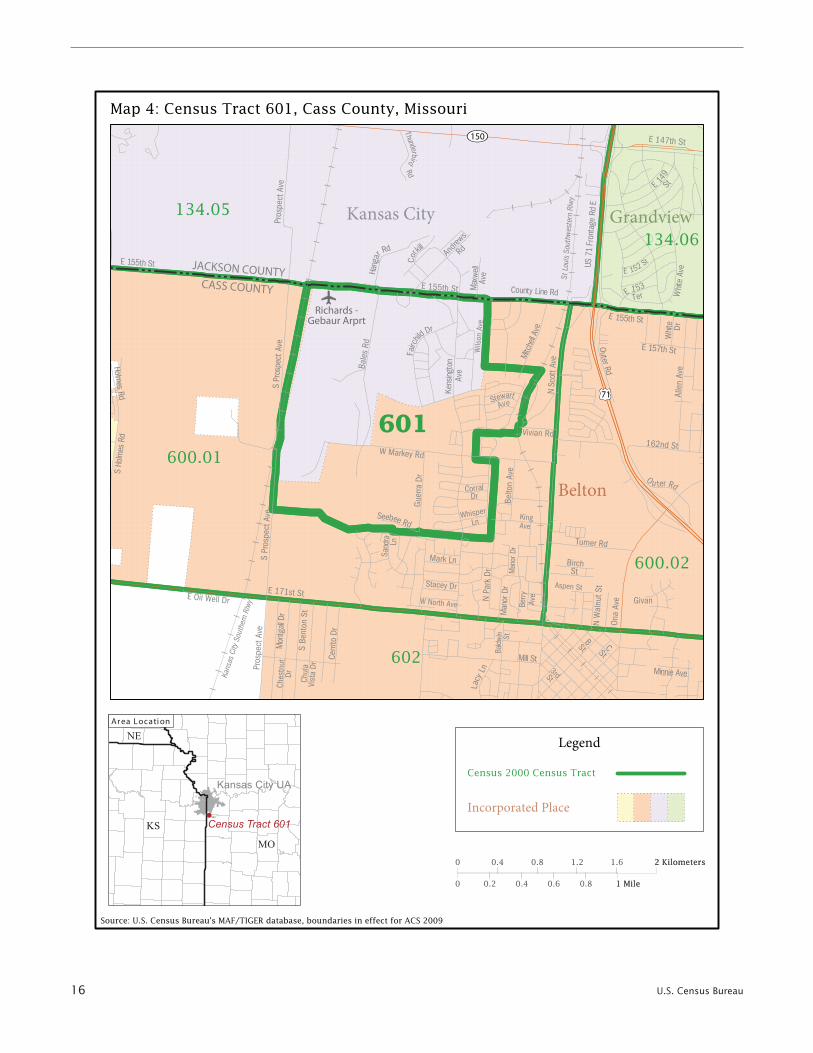
Census Tract 601 in Cass County Missouri, the tract with the most equal measured income

Table 7. Census Tracts With the Highest and Lowest Measured Household Income Inequality: 2005–2009

Name of areaHouse-

holds PopulationHousing

units Gini indexStandard

error Urbanized area1

Tracts with the highest income inequalityCensus Tract 17, Hamilton County, Ohio . . . . . . . . . . . . . . 321 630 894 0.833 0.1024 CincinnatiCensus Tract 20, Kent County, Michigan . . . . . . . . . . . . . . 1,060 1,936 1,429 0.798 0.0430 Grand RapidsCensus Tract 207.01, Bell County, Texas . . . . . . . . . . . . . . 631 1,226 868 0.770 0.1504 TempleCensus Tract 7, Travis County, Texas . . . . . . . . . . . . . . . . . 592 964 830 0.764 0.1308 AustinCensus Tract 9506, Rusk County, Texas . . . . . . . . . . . . . . 754 1,846 1,052 0.759 0.0965 -none-Census Tract 1018, Tarrant County, Texas . . . . . . . . . . . . . 941 1,165 1,092 0.755 0.0405 Fort WorthCensus Tract 1301, Allegheny County, Pennsylvania . . . . 983 2,113 1,293 0.728 0.1337 PittsburghCensus Tract 122.05, Boulder County, Colorado . . . . . . . . 1,603 2,894 1,876 0.724 0.0860 BoulderCensus Tract 126, Tuscaloosa County, Alabama . . . . . . . . 839 2,171 1,083 0.718 0.0405 TuscaloosaCensus Tract 9706, Richmond County, North Carolina . . . 1,634 4,550 1,860 0.716 0.1055 Rockingham

United States census tract averages . . . . . . . . . . . . . . . 1,812 4,825 2,054 0 .467 (X) (X)

Tracts with the lowest income inequalityCensus Tract 85.24, Adams County, Colorado . . . . . . . . . 2,292 7,419 2,435 0.231 0.0134 Denver-AuroraCensus Tract 98.29, Jefferson County, Colorado. . . . . . . . 732 2,249 732 0.230 0.0256 Denver-AuroraCensus Tract 115, Richland County, South Carolina . . . . . 958 13,063 1,481 0.229 0.0201 ColumbiaCensus Tract 32.03, Kern County, California . . . . . . . . . . . 750 2,542 789 0.228 0.0266 BakersfieldCensus Tract 70.82, Arapahoe County, Colorado . . . . . . . 1,341 4,686 1,341 0.227 0.0163 Denver-AuroraCensus Tract 5, Wayne County, North Carolina . . . . . . . . . 924 3,737 1,544 0.222 0.0247 Goldsboro

Census Tract 4064.02, Los Angeles County, California . . . 606 2,191 606 0.221 0.0243Los Angeles-Long Beach-Santa Ana

Census Tract 1135.26, Salt Lake County, Utah . . . . . . . . . 1,262 4,977 1,279 0.215 0.0148 Salt Lake CityCensus Tract 9702, Meade County, Kentucky . . . . . . . . . . 903 2,811 1,602 0.213 0.0295 -none-Census Tract 601, Cass County, Missouri . . . . . . . . . . . . . 686 1,886 719 0.204 0.0191 Kansas City

(X) Not applicable.

Notes: None of the Gini measures for the highest (lowest) inequality tracts are statistically different from any others in the list of highest (lowest) inequality tracts, or from that for numerous other tracts not listed. For example, the 90 percent confidence interval for the Gini index for Census Tract 17 Hamilton County Ohio is 0.665 to 1.000, and the 90 percent confidence interval for the Gini index for Census Tract 601 Cass County Missouri is 0.173 to 0.236. Table excludes tracts with fewer than 50 interviews in the 2005–2009 period.

1 Census Tract 9506, Rusk County, Texas is between Carthage and Henderson. Rockingham is an urban cluster, not an urbanized area. Census Tract 9702, Meade County, Kentucky is southwest of Louisville.



KY

Cincinnati UA

OHIN

Census Tract 17

Area Location


KS

Kansas City UA

NE

MO

Census Tract 601

Ar ea Locati on


distribution, is very different from Census Tract 17 in Hamilton County Ohio (see Map 4). While it is also part of an urbanized area (Kansas City in this case), it is suburban rather than center city, located in the northwest corner of Cass County near Belton MO and the former Richards-Gebaur Air Force Base, and south of the county in which most of Kansas City is found (Jackson County MO). Only 17 percent of its households were ones in which the householder is female with no husband pres-ent; 28 percent of the households consist of an individual living alone and 46 percent are married-couple families. The tract is racially and ethnically mixed, with 72 percent of the tract’s population being Non-Hispanic White, 14 percent reporting themselves as Black or African-American, and 10 percent as Hispanic. There’s even a sizeable Samoan representation (3 percent). Unemployment there is low (3

percent), and income is distributed over much of the range (only 2 percent received under $10,000 while 88 percent received between $25,000 and $74,999). None of the housing was built before 1939; 70 percent was built between 1950 and 1969 and the vacancy rate was 5 percent.

This univariate analysis above sug-gests that perhaps those relatively well-off want to live mainly with those who are also relatively well-off, and those who are toward the lower end of the income spectrum don’t have that choice and live in areas with high inequality.

MULTIVARIATE ANALYSIS OF CENSUS TRACTS

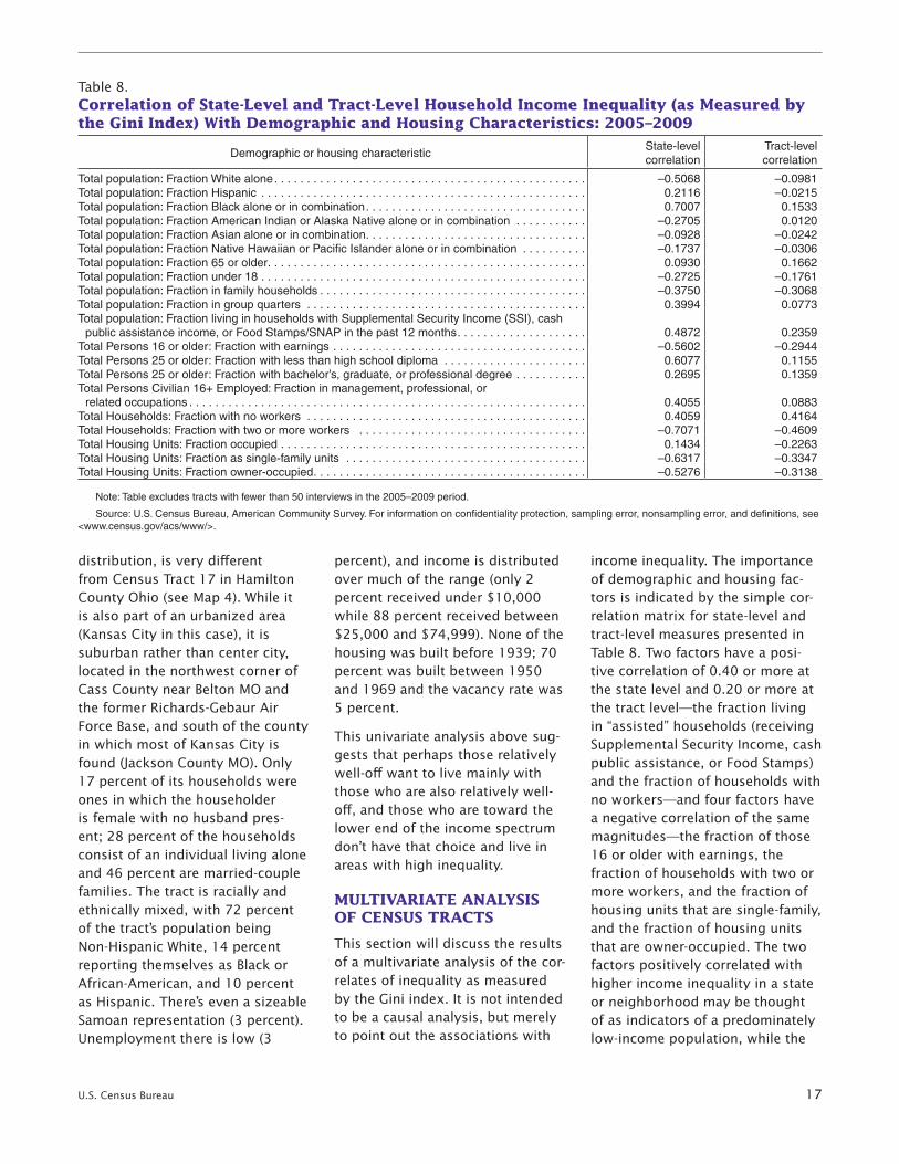
This section will discuss the results of a multivariate analysis of the cor-relates of inequality as measured by the Gini index. It is not intended to be a causal analysis, but merely to point out the associations with

income inequality. The importance of demographic and housing fac-tors is indicated by the simple cor-relation matrix for state-level and tract-level measures presented in Table 8. Two factors have a posi-tive correlation of 0.40 or more at the state level and 0.20 or more at the tract level—the fraction living in “assisted” households (receiving Supplemental Security Income, cash public assistance, or Food Stamps) and the fraction of households with no workers—and four factors have a negative correlation of the same magnitudes—the fraction of those 16 or older with earnings, the fraction of households with two or more workers, and the fraction of housing units that are single-family, and the fraction of housing units that are owner-occupied. The two factors positively correlated with higher income inequality in a state or neighborhood may be thought of as indicators of a predominately low-income population, while the

Table 8. Correlation of State-Level and Tract-Level Household Income Inequality (as Measured by the Gini Index) With Demographic and Housing Characteristics: 2005–2009

Demographic or housing characteristicState-level correlation

Tract-level correlation

Total population: Fraction White alone . . . . . . . . . . . . . . . . . . . . . . . . . . . . . . . . . . . . . . . . . . . . . . . . –0.5068 –0.0981Total population: Fraction Hispanic . . . . . . . . . . . . . . . . . . . . . . . . . . . . . . . . . . . . . . . . . . . . . . . . . . 0.2116 –0.0215Total population: Fraction Black alone or in combination . . . . . . . . . . . . . . . . . . . . . . . . . . . . . . . . . . 0.7007 0.1533Total population: Fraction American Indian or Alaska Native alone or in combination . . . . . . . . . . . –0.2705 0.0120Total population: Fraction Asian alone or in combination . . . . . . . . . . . . . . . . . . . . . . . . . . . . . . . . . . –0.0928 –0.0242Total population: Fraction Native Hawaiian or Pacific Islander alone or in combination . . . . . . . . . . –0.1737 –0.0306Total population: Fraction 65 or older . . . . . . . . . . . . . . . . . . . . . . . . . . . . . . . . . . . . . . . . . . . . . . . . . 0.0930 0.1662Total population: Fraction under 18 . . . . . . . . . . . . . . . . . . . . . . . . . . . . . . . . . . . . . . . . . . . . . . . . . . –0.2725 –0.1761Total population: Fraction in family households . . . . . . . . . . . . . . . . . . . . . . . . . . . . . . . . . . . . . . . . . –0.3750 –0.3068Total population: Fraction in group quarters . . . . . . . . . . . . . . . . . . . . . . . . . . . . . . . . . . . . . . . . . . . 0.3994 0.0773Total population: Fraction living in households with Supplemental Security Income (SSI), cash

public assistance income, or Food Stamps/SNAP in the past 12 months . . . . . . . . . . . . . . . . . . . . 0.4872 0.2359Total Persons 16 or older: Fraction with earnings . . . . . . . . . . . . . . . . . . . . . . . . . . . . . . . . . . . . . . . –0.5602 –0.2944Total Persons 25 or older: Fraction with less than high school diploma . . . . . . . . . . . . . . . . . . . . . . 0.6077 0.1155Total Persons 25 or older: Fraction with bachelor’s, graduate, or professional degree . . . . . . . . . . . 0.2695 0.1359Total Persons Civilian 16+ Employed: Fraction in management, professional, or

related occupations . . . . . . . . . . . . . . . . . . . . . . . . . . . . . . . . . . . . . . . . . . . . . . . . . . . . . . . . . . . . . 0.4055 0.0883Total Households: Fraction with no workers . . . . . . . . . . . . . . . . . . . . . . . . . . . . . . . . . . . . . . . . . . . 0.4059 0.4164Total Households: Fraction with two or more workers . . . . . . . . . . . . . . . . . . . . . . . . . . . . . . . . . . . –0.7071 –0.4609Total Housing Units: Fraction occupied . . . . . . . . . . . . . . . . . . . . . . . . . . . . . . . . . . . . . . . . . . . . . . . 0.1434 –0.2263Total Housing Units: Fraction as single-family units . . . . . . . . . . . . . . . . . . . . . . . . . . . . . . . . . . . . . –0.6317 –0.3347Total Housing Units: Fraction owner-occupied . . . . . . . . . . . . . . . . . . . . . . . . . . . . . . . . . . . . . . . . . . –0.5276 –0.3138

Note: Table excludes tracts with fewer than 50 interviews in the 2005–2009 period.



four factors associated with lower income inequality are more indica-tors of a higher-income population. (Reflecting the scatter plots shown in Figure 3 for places, correlations of the Gini index with median household income are –0.12 at the state level and –0.22 at the tract level.)

The highest correlations of the Gini index at the state level are with the fraction Black alone or in combination (0.70) and the fraction with two or more workers (–0.71), followed by the fraction of housing units as single-family units (–0.63) and fraction with less than high school diploma (0.61). At the tract

level, the highest correlations are the fraction with no workers (0.42) and the fraction with two or more workers (–0.46).

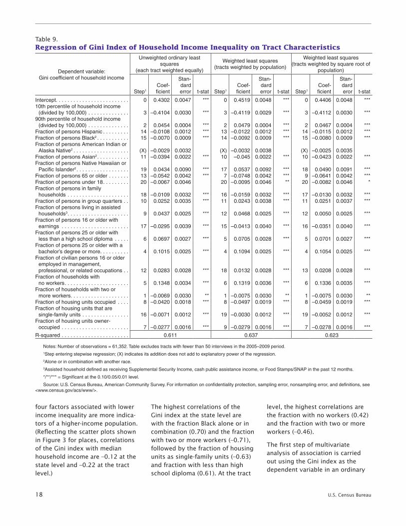
The first step of multivariate analysis of association is carried out using the Gini index as the dependent variable in an ordinary

Table 9. Regression of Gini Index of Household Income Inequality on Tract Characteristics

Dependent variable:Gini coefficient of household income

Unweighted ordinary least squares

(each tract weighted equally)

Weighted least squares(tracts weighted by population)

Weighted least squares(tracts weighted by square root of

population)

Step1

Coef-ficient

Stan-dard error t-stat Step1

Coef-ficient

Stan-dard error t-stat Step1

Coef-ficient

Stan-dard eror t-stat

Intercept . . . . . . . . . . . . . . . . . . . . . . . . . 0 0.4302 0.0047 *** 0 0.4519 0.0048 *** 0 0.4406 0.0048 ***10th percentile of household income

(divided by 100,000) . . . . . . . . . . . . . . 3 –0.4104 0.0030 *** 3 –0.4119 0.0029 *** 3 –0.4112 0.0030 ***90th percentile of household income

(divided by 100,000) . . . . . . . . . . . . . . 2 0.0454 0.0004 *** 2 0.0479 0.0004 *** 2 0.0467 0.0004 ***Fraction of persons Hispanic . . . . . . . . . 14 –0.0108 0.0012 *** 13 –0.0122 0.0012 *** 14 –0.0115 0.0012 ***Fraction of persons Black2 . . . . . . . . . . . 15 –0.0070 0.0009 *** 14 –0.0092 0.0009 *** 15 –0.0080 0.0009 ***Fraction of persons American Indian or

Alaska Native2 . . . . . . . . . . . . . . . . . . . (X) –0.0029 0.0032 (X) –0.0032 0.0038 (X) –0.0025 0.0035Fraction of persons Asian2 . . . . . . . . . . . 11 –0.0394 0.0022 *** 10 –0.045 0.0022 *** 10 –0.0423 0.0022 ***Fraction of persons Native Hawaiian or

Pacific Islander2 . . . . . . . . . . . . . . . . . . 19 0.0434 0.0090 *** 17 0.0537 0.0092 *** 18 0.0490 0.0091 ***Fraction of persons 65 or older . . . . . . . 13 –0.0542 0.0042 *** 7 –0.0748 0.0042 *** 9 –0.0641 0.0042 ***Fraction of persons under 18 . . . . . . . . . 20 –0.0067 0.0046 20 –0.0095 0.0046 ** 20 –0.0082 0.0046 *Fraction of persons in family

households . . . . . . . . . . . . . . . . . . . . . 18 –0.0109 0.0032 *** 16 –0.0159 0.0032 *** 17 –0.0130 0.0032 ***Fraction of persons in group quarters . . 10 0.0252 0.0035 *** 11 0.0243 0.0038 *** 11 0.0251 0.0037 ***Fraction of persons living in assisted

households3 . . . . . . . . . . . . . . . . . . . . . 9 0.0437 0.0025 *** 12 0.0468 0.0025 *** 12 0.0050 0.0025 ***Fraction of persons 16 or older with

earnings . . . . . . . . . . . . . . . . . . . . . . . 17 –0.0295 0.0039 *** 15 –0.0413 0.0040 *** 16 –0.0351 0.0040 ***Fraction of persons 25 or older with

less than a high school diploma . . . . . 6 0.0697 0.0027 *** 5 0.0705 0.0028 *** 5 0.0701 0.0027 ***Fraction of persons 25 or older with a

bachelor’s degree or more. . . . . . . . . . 4 0.1015 0.0025 *** 4 0.1094 0.0025 *** 4 0.1054 0.0025 ***Fraction of civilian persons 16 or older

employed in management, professional, or related occupations . . 12 0.0283 0.0028 *** 18 0.0132 0.0028 *** 13 0.0208 0.0028 ***

Fraction of households with no workers . . . . . . . . . . . . . . . . . . . . . . 5 0.1348 0.0034 *** 6 0.1319 0.0036 *** 6 0.1336 0.0035 ***

Fraction of households with two or more workers . . . . . . . . . . . . . . . . . . . . 1 –0.0069 0.0030 ** 1 –0.0075 0.0030 ** 1 –0.0075 0.0030 **

Fraction of housing units occupied . . . . 8 –0.0420 0.0018 *** 8 –0.0497 0.0019 *** 8 –0.0459 0.0019 ***Fraction of housing units that are

single-family units . . . . . . . . . . . . . . . . 16 –0.0071 0.0012 *** 19 –0.0030 0.0012 *** 19 –0.0052 0.0012 ***Fraction of housing units owner-

occupied . . . . . . . . . . . . . . . . . . . . . . . 7 –0.0277 0.0016 *** 9 –0.0279 0.0016 *** 7 –0.0278 0.0016 ***

R-squared . . . . . . . . . . . . . . . . . . . . . . . 0.611 0.637 0.623

Notes: Number of observations = 61,352. Table excludes tracts with fewer than 50 interviews in the 2005–2009 period.1Step entering stepwise regression; (X) indicates its addition does not add to explanatory power of the regression.2Alone or in combination with another race.3Assisted household defined as receiving Supplemental Security Income, cash public assistance income, or Food Stamps/SNAP in the past 12 months.

*/**/*** = Significant at the 0.10/0.05/0.01 level.



least squares (OLS) regression on all the demographic characteristics included in Table 8, and all tracts are weighted equally. Two further extensions are also reported: (1) a stepwise OLS regression, allowing the most influential independent variables to enter one by one; and (2) weighted least squares (WLS) regressions; stepwise WLS results are also reported. The weights for WLS regressions were designed to give more weight to larger tracts wherein the Gini coefficients are expected to be more reliable. One set of weights uses the population directly and the second set uses the square root of population; all weights are adjusted to sum to the number of tracts (that is, the same sum of the implicit weights used in the OLS regressions).

Table 9 shows the regression results for all six approaches. The fit (R2) is reasonably high for a cross-sectional regression; these independent variables explain 61 percent of the variation in the Gini index using OLS, and slightly more (64 and 62 percent) using the two WLS approaches.

In the OLS regression, there are only two variables that have no independent association with the Gini coefficient—the fraction American Indian or Alaska Native (AIAN), and the fraction of the population under 18.26 However, in the two WLS regressions, only the fraction AIAN does not contribute to the explanatory power of the independent variables. Below, the

26 The latter is significant only at the 0.13 level.

magnitude of the association of the independent variables with the Gini coefficient is discussed using the regression equation with the best fit—the WLS regression using the total population weights.

The three most influential indepen-dent variables affecting the Gini coefficient—the ones entering the stepwise regression first—are the fraction with two or more workers, and the two income variables (the 10th and the 90th percentiles of income). Together they explain 57 percent of the variance in the Gini index by tract that is, almost 90 percent of the 64 percent explained by the independent variables.

All estimated coefficients are converted to percentage changes evaluated at the means of all the

Table 10. Effects of Change in Tract Characteristics on Gini Index of Household Income Inequality of a One Standard Deviation Change in the Characteristic

Demographic or housing characteristic

MeanStandard deviation

Implied change in

Gini coefficient

10th percentile of household income (divided by 100,000) . . . . . . . . . . . . . . . . . . . . . . . . . . . . . . . . 0.159 0.093 –0.03890th percentile of household income (divided by 100,000) . . . . . . . . . . . . . . . . . . . . . . . . . . . . . . . . 1.317 0.739 0.034Fraction of persons Hispanic . . . . . . . . . . . . . . . . . . . . . . . . . . . . . . . . . . . . . . . . . . . . . . . . . . . . . . . 0.135 0.201 –0.002Fraction of persons Black1 . . . . . . . . . . . . . . . . . . . . . . . . . . . . . . . . . . . . . . . . . . . . . . . . . . . . . . . . . 0.137 0.222 –0.002Fraction of persons American Indian or Alaska Native1 . . . . . . . . . . . . . . . . . . . . . . . . . . . . . . . . . . . 0.016 0.050 –Fraction of persons Asian1 . . . . . . . . . . . . . . . . . . . . . . . . . . . . . . . . . . . . . . . . . . . . . . . . . . . . . . . . . 0.045 0.087 –0.003Fraction of persons Native Hawaiian or Pacific Islander1 . . . . . . . . . . . . . . . . . . . . . . . . . . . . . . . . . . 0.003 0.019 0.001Fraction of persons 65 or older . . . . . . . . . . . . . . . . . . . . . . . . . . . . . . . . . . . . . . . . . . . . . . . . . . . . . 0.135 0.069 –0.004Fraction of persons under 18 . . . . . . . . . . . . . . . . . . . . . . . . . . . . . . . . . . . . . . . . . . . . . . . . . . . . . . . 0.240 0.065 –Fraction of persons in family households . . . . . . . . . . . . . . . . . . . . . . . . . . . . . . . . . . . . . . . . . . . . . 0.809 0.125 –0.001Fraction of persons in group quarters . . . . . . . . . . . . . . . . . . . . . . . . . . . . . . . . . . . . . . . . . . . . . . . . 0.022 0.065 0.002Fraction of persons living in assisted households2 . . . . . . . . . . . . . . . . . . . . . . . . . . . . . . . . . . . . . . 0.143 0.120 0.005Fraction of persons 16 or older with earnings . . . . . . . . . . . . . . . . . . . . . . . . . . . . . . . . . . . . . . . . . . 0.682 0.094 –0.003Fraction of persons 25 or older with less than a high school diploma . . . . . . . . . . . . . . . . . . . . . . . 0.160 0.118 0.008Fraction of persons 25 or older with a bachelor’s degree or more . . . . . . . . . . . . . . . . . . . . . . . . . . . 0.263 0.178 0.018Fraction of civilian persons 16 or older employed in management, professional, or

related occupations . . . . . . . . . . . . . . . . . . . . . . . . . . . . . . . . . . . . . . . . . . . . . . . . . . . . . . . . . . . . . 0.332 0.143 0.004Fraction of households with no workers . . . . . . . . . . . . . . . . . . . . . . . . . . . . . . . . . . . . . . . . . . . . . . 0.268 0.105 0.014Fraction of households with two or more workers . . . . . . . . . . . . . . . . . . . . . . . . . . . . . . . . . . . . . . . 0.345 0.105 –0.001Fraction of housing units occupied . . . . . . . . . . . . . . . . . . . . . . . . . . . . . . . . . . . . . . . . . . . . . . . . . . 0.887 0.097 –0.004Fraction of housing units that are single-family units . . . . . . . . . . . . . . . . . . . . . . . . . . . . . . . . . . . . 0.685 0.236 –0.002Fraction of housing units owner-occupied . . . . . . . . . . . . . . . . . . . . . . . . . . . . . . . . . . . . . . . . . . . . . 0.666 0.218 –0.006

– Represents or rounds to zero.

Notes: The effect is evaluated for a change from one-half a standard deviation below to one-half above, at the means for the other independent variables using the population-weighted least squares regression.

1 Alone or in combination with another race.2 Assisted household defined as receiving Supplemental Security Income, cash public assistance income, or Food Stamps/SNAP in the past 12 months.



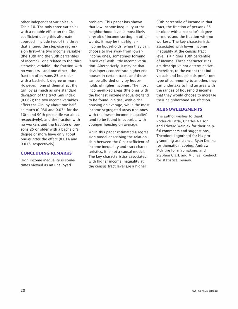
other independent variables in Table 10. The only three variables with a notable effect on the Gini coefficient using this alternate approach include two of the three that entered the stepwise regres-sion first—the two income variable (the 10th and the 90th percentiles of income)—one related to the third stepwise variable—the fraction with no workers—and one other—the fraction of persons 25 or older with a bachelor’s degree or more. However, none of them affect the Gini by as much as one standard deviation of the tract Gini index (0.062); the two income variables affect the Gini by about one-half as much (0.038 and 0.034 for the 10th and 90th percentile variables, respectively), and the fraction with no workers and the fraction of per-sons 25 or older with a bachelor’s degree or more have only about one-quarter the effect (0.014 and 0.018, respectively).

CONCLUDING REMARKS

High income inequality is some-times viewed as an unalloyed

problem. This paper has shown that low income inequality at the neighborhood level is most likely a result of income sorting. In other words, it may be that higher-income households, when they can, choose to live away from lower-income ones, sometimes forming “enclaves” with little income varia-tion. Alternatively, it may be that developers concentrate higher-end houses in certain tracts and those can be afforded only by house-holds of higher incomes. The most income-mixed areas (the ones with the highest income inequality) tend to be found in cities, with older housing on average, while the most income-segregated areas (the ones with the lowest income inequality) tend to be found in suburbs, with younger housing on average.

While this paper estimated a regres-sion model describing the relation-ship between the Gini coefficient of income inequality and tract charac-teristics, it is not a causal model. The key characteristics associated with higher income inequality at the census tract level are a higher

90th percentile of income in that tract, the fraction of persons 25 or older with a bachelor’s degree or more, and the fraction with no workers. The key characteristic associated with lower income inequality at the census tract level is a higher 10th percentile of income. These characteristics are descriptive not determinative. Therefore, to the extent that indi-viduals and households prefer one type of community to another, they can undertake to find an area with the ranges of household income that they would choose to increase their neighborhood satisfaction.

ACKNOWLEDGMENTS

The author wishes to thank Roderick Little, Charles Nelson, and Edward Welniak for their help-ful comments and suggestions, Theodore Logothetti for his pro-gramming assistance, Ryan Kenma for thematic mapping, Andrew McIntire for mapmaking, and Stephen Clark and Michael Roebuck for statistical review.


REFERENCES

Benabou, Roland. 1996. “Heterogeneity, Stratification, and Growth: Macroeconomic Implications of Community Structure and School Finance.” American Economic Review Vol. 86, 584–609.

Bishaw, Alemayehu and Jessica Semega. 2008. Income, Earnings, and Poverty Data From the 2007 American Community Survey. U.S. Census Bureau American Community Survey Reports ACS-09, August.

DeNavas-Walt, Carmen, Bernadette D. Proctor, and Jessica C. Smith. 2010. Income, Poverty, and Health Insurance Coverage in the United States: 2009. U.S. Census Bureau Current Population Reports P60-238, September.

Hardman, Anna and Yannis M. Ioannides. 2004. “Neighbors’ Income Distribution: Economic Segregation and Mixing in US Urban Neighborhoods.” Journal of Housing Economics Vol. 13, 368–82.

Kain, John F. 1968. “Housing Segregation, Negro Employment, and Metropolitan Decentralization.” Quarterly Journal of Economics Vol. 82, No. 2, May, 175–97.

Jones, Arthur F. and Daniel H. Weinberg. 2000. The Changing Shape of the Nation’s Income Distribution: 1947–1998. U.S. Census Bureau Current Population Reports P60-204, June.

Paddock, Susan M., Greg Ridgeway, Rongheng Lin, and Thomas A. Louis. 2006. “Flexible Distributions for Triple-Goal Estimates in Two-Stage Hierarchical Models.” Computational Statistics and Data Analysis Vol. 50, No. 11, July, 3243–62.

Thurow, Lester C. 1971. “The Income Distribution as a Pure Public Good.” Quarterly Journal of Economics Vol. 85, No. 2, May, 327–36.

Tiebout, Charles M. 1956. “A Pure Theory of Local Public Expenditures.” Journal of Political Economy Vol. 64, 416–24.

Watson, Tara. 2009. “Inequality and the Measurement of Residential Segregation by Income in American Neighborhoods.” Review of Income and Wealth Series 55, No. 3, September, 820–44.

Weinberg, Daniel H. 1996. A Brief Look at Postwar U.S. Income Inequality. U.S. Census Bureau Current Population Reports P60-191, June.

Wheeler, Christopher H. 2008. “Urban Decentralization and Income Inequality: Is Sprawl Associated with Rising Income Segregation Across Neighborhoods?” Federal Reserve Bank of St. Louis Regional Economic Development Vol. 4, No. 1, 41–57.

Wilson, William J. 1987. The Truly Disadvantaged: The Inner City, the Underclass, and Public Policy. Chicago: University of Chicago Press.

u.s. neighborhood income inequality in the 2005-2009 … · u.s. department of commerce economics...

Documents