US–Mexico border tourism and day trips:an aberration in globalization?

John Berdell1 • Animesh Ghoshal1

Received: 21 February 2015 / Revised: 3 September 2015 /Accepted: 19 September 2015 /

Published online: 26 November 2015

� The Author(s) 2015. This article is published with open access at Springerlink.com

Abstract We examine the influence of two distinct regime changes in US border

security on the number of persons traveling from the US into Mexico on day trips.

In contrast to increases in overall US tourism to Mexico and rapidly growing trade

linkages, day trips to Mexico fell by over 20 % between 2000 and 2012. In the

popular press, the reduction in short visits is widely attributed to a rising tide of

violence in the Mexican border states, more specifically to a rise in the rate of

homicides as a result of the emergence, or radical transformation, of a drug war in

Mexico. We show that changes in the US border regime caused a large reduction of

day trips and border tourism, and in doing so had a large negative effect on the

Mexican border. We situate this result within the literature devoted to analyzing the

effects of changes in international documents on tourist flows.

Keywords Tourism � Constraints to travel � Regional integration � Border security

JEL Classification F15 � F52 � R21

1 Introduction: Globalization and the border

If globalization is conceived as the movement towards a borderless world, the

physical interface between the US and Mexico can only be a study in contradictions.

On the one hand, flows of goods have continued to increase along with, if not faster

than, the general trend towards greater vertical specialization in the world economy.

China’s entry into the world economy considerably dampened the hopes that

& John Berdell

jberdell@depaul.edu

1 DePaul University, Chicago, IL, USA

123

Lat Am Econ Rev (2015) 24:15

DOI 10.1007/s40503-015-0023-9

NAFTA had raised for Mexican export performance, but by now there are clear

signs that US–Mexican integration continues apace. Financial integration has

clearly accompanied the integration of trade and production (Lahrech and Sylwester

2013). Of course barriers to the movement of people have not fallen at the same

pace, and remain politically fraught. Rivers of ink have been devoted to the causes,

consequences and regulation of migration over the border, but the very shortest of

trans-border trips, in which someone comes and goes within the same day—perhaps

within a few hours—have gone relatively unattended. On one level this is quite

understandable since such short trips are necessarily confined to the border region,

unlike immigration which has effects throughout both nations. Yet changes in the

regulations governing very short trips are of tremendous local consequence. They

also have wider national consequence to the extent that the communities that

constitute the border loom increasingly large within their national economies and

populations.

Border regions can either be vibrant areas of commercial interchange that

contribute to the dynamism of their larger economies, or at the other extreme, they

can be relatively isolated, peripheral areas where stagnation reduces national

progress. In a much cited conceptual paper on cross-border contact, based primarily

on the US–Mexican border, Martinez (1994) categorizes borderlands into four

categories: alienated, where due to hostility cross-border interaction is severely

restricted; co-existent, with limited binational integration; interdependent, where a

mutually beneficial economic system is created through the flow of resources and

people across the border; and integrated, where barriers to trade and human

movements have been eliminated, and the border economies are functionally

merged. In the spirit of Martinez’s view of an integrated border, Cooper and

Rumford (2013) argue that borders must be regarded as mechanisms of connectivity

and encounter rather than markers of division. An example of such a border is

discussed in Prokkola’s (2010) study of the transition of the internal border regions

of the European Union. Focusing on tourism in the frontier between Finland and

Sweden, Prokkola finds that border permeability has contributed to dissolution of

mental boundaries in the region.

In this paper, we examine two periods that experienced dramatic changes in the

rules and regulations governing movement between the US and Mexico. The rules

concern the documentation that US residents need to produce in order to reenter the

US from Mexico. We seek to establish whether these changes in regulations are

important in explaining the reduction, over the past two decades, in day trips from

the US into Mexico (and back). This reduction in day trips stands in marked contrast

to the increasing volumes of goods and services trade, as well as tourism that is not

associated with the border. We begin (in Sect. 2) with a very short discussion of the

importance of the border region to the Mexican economy, and the role that short

visits may play in the border region’s economic and social development. We then

provide (in Sect. 3) a provisional outline of the two changes to the border crossing

regulatory regime that have been of considerable consequence for recorded cross-

border day trips. We also briefly discuss a critical confounding factor, namely the

dramatic increase in the homicide rate within the Mexican border states. Sections 4

and 5 present estimates of the impact of the two regulatory regime changes on day

15 Page 2 of 18 Lat Am Econ Rev (2015) 24:15

123

trips. The conclusion summarizes the implications of our analysis for the growth

and transformation of the border economy and the tourism sector.

2 Tourism in ‘‘la Frontera Norte’’

As in many developing economies, tourism has had a significant role in Mexico’s

economic development.1 In one of the first empirical investigations of tourism in

Mexico, Stronge and Redman (1982) found tourism along the border by Americans

was income and price elastic, while tourism in the interior was inelastic with respect

to Mexican prices. Clancy (1999), in a study primarily focused on the political

economy of the role of tourism in economic development, provides useful data on

the growth of tourism in Mexico in the period 1970–1994, and concludes that the

state played a crucial role in its growth. Of particular interest to our paper, he

recognizes that when developing countries promote tourism, ‘‘they are, in effect,

embracing greater integration into the world economy’’ (Clancy 1999, p. 2).

We might also briefly mention some studies of border tourism in other countries

which are germane to our analysis. Hampton (2010) examined the impact of tourism

from Singapore on border communities in both southern Malaysia and western

Indonesia, and concludes that it generated employment, income, and local economic

linkages, with cross-border ethnic ties playing an important role. David et al. (2011)

focus on the border regions of Hungary, and find, not surprisingly, that accession to

the EU had a positive impact on cross-border tourism. In a survey of border tourism

in the Balkans, Lagiewski and Revelas (2004) find that the most commonly

identified problems in expanding tourism revolve around the ease and convenience

of border crossing.

In 2012, the travel and tourism industry contributed 1272 billion pesos to

Mexican GDP (8.4 % of the total), and employed 2.95 million workers, 6.3 % of

total employment (INEGI).2 The government of Mexico keeps detailed figures on

the number of tourists (and their expenditure), and breaks down the total into several

categories, based on the length of their stay and where they travel. The official

categories are:

Excursionistas Fronterizos: international visitors who come only for a day trip

and remain in the border zone.

Pasajeros en Crucero: cruise ship passengers (who are not considered tourists

because they do not spend the night in Mexico).

Excursionistas Internacionales: the sum of border visitors and cruise ship

visitors.

1 The contributions of tourism to economic development have been well documented, and development

agencies have set up units to promote it (Brohman 1996; Sharpley and Telfer 2002). The World Tourism

Organization, established in 1975, became a UN specialized agency in 2003. The World Bank established

a Tourism Projects Department in 1969. Both institutions currently view tourism as having a major role in

Millennium Development Goals (Mann 2005).2 Mexico was ranked No. 2 among Latin American countries, in the World Economic Forum’s report on

travel and tourism competitiveness (Blanke and Chiesa 2013).

Lat Am Econ Rev (2015) 24:15 Page 3 of 18 15

123

Turismo al Interior: international visitors who stay overnight, and go beyond the

border zone.

Turismo Fronterizo: international visitors who stay overnight, but remain in the

border zone.

Turismo al Interior: international visitors who stay overnight outside of the

border zone.

Turistas Internacionales: international visitors who stay overnight in Mexico.

Visitantes Internacionales a Mexico: all visitors who come to Mexico and stay for

no more than a year.3

Tourism has been particularly important in Mexico’s border states; e.g., the first

detailed study showed that in 1994, it accounted for 9.4 % of output, 8.6 % of

employment, and 17 % of investment in Baja California (Secretarıa de Turismo-

REDES Sociedad Civil 1996).4 After the initiation of NAFTA, tourism expanded

rapidly. While tourist destinations further south are better known, historically about

80 % of tourists stayed within the six Mexican border states. The vast majority of

these are excursionistas or –as we will call them—day trips. The motivations behind

day trips vary widely but prominently include family visits, work, and cross-border

shopping. Prices of goods and services are sometimes quite different across the

border, with pharmaceuticals and medical services notably attracting customers

from the North. Day trips also reflect family visits and weekend leisure activity. The

role of cross-border shopping can be crucial in frontier cities, and while we have not

come across quantitative measures of their significance on the Mexican side of the

border, studies on the US side estimate that Mexican shoppers account for 40–45 %

of retail purchases in Laredo, 35–40 % in McAllen, 30–35 % in Brownsville, and

10–15 % in El Paso (Coronado and Phillips 2012).

While the United States has long had concerns about illegal immigration from

Mexico,5 the border was quite easy to cross for US residents. A driver’s license and

an oral declaration of citizenship generally sufficed, and for those who lived in

frontier cities, crossing the border to shop was little different from shopping in an

adjacent suburb.6 By the end of the twentieth century, the border had become quite

‘‘thin’’, and the economies on each side of the border were becoming increasingly

integrated. As noted by Thompson (2008), ‘‘…a common border culture…was

helping to integrate northern Mexico with the southern US’’. As a result Mexico’s

northern border zone or ‘‘la frontera norte’’ has been an important contributor to

Mexican growth. The six Mexican states that border the US capture a large and

relatively prosperous part of Mexico. By 2013 the six states contained 17 % of

Mexico’s population and produced 22.5 % of its GDP. They also exhibit relatively

3 We focus on the number of day trips, Excursionistas Fronterizos, which is a contributory element of

both Turismo Fronterizo and Visitantes Internacionales a Mexico.4 Comparable figures for the Mexican economy as whole were 5.7, 5, and 11.2 %.5 In September 2001, there were 9061 US border patrol agents deployed along the Mexican border, while

331 were at the Canadian border (Transactional Records Access Clearinghouse 2006).6 One of the authors recalls, while living in Laredo (Texas), easily walking across the bridge to Nuevo

Laredo for lunch and shopping.

15 Page 4 of 18 Lat Am Econ Rev (2015) 24:15

123

high human development indices and contain relatively fewer workers earning the

minimum salary (Bringas Rabago 2005).

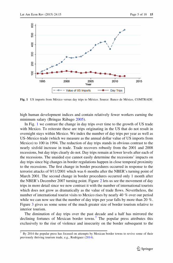
In Fig. 1 we contrast the change in day trips over time to the growth of US trade

with Mexico. To reiterate these are trips originating in the US that do not result in

overnight stays within Mexico. We index the number of day trips per year as well as

US–Mexico trade (which we measure as the annual dollar value of US imports from

Mexico) to 100 in 1994. The reduction of day trips stands in obvious contrast to the

nearly sixfold increase in trade. Trade recovers robustly from the 2001 and 2008

recessions, but day trips clearly do not. Day trips remain at lower levels after each of

the recessions. The unaided eye cannot easily determine the recessions’ impacts on

day trips since big changes in border regulations happen in close temporal proximity

to the recessions. The first change in border procedures occurred in response to the

terrorist attacks of 9/11/2001 which was 6 months after the NBER’s turning point of

March 2001. The second change in border procedures occurred only 1 month after

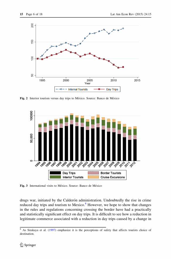
the NBER’s December 2007 turning point. Figure 2 lets us see the movement of day

trips in more detail since we now contrast it with the number of international tourists

which does not grow as dramatically as the value of trade flows. Nevertheless, the

number of international tourist visits to Mexico rises by nearly 40 % over our period

while we can now see that the number of day trips per year falls by more than 20 %.

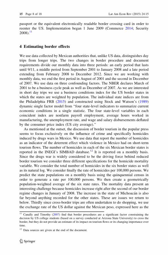
Figure 3 gives us some sense of the much greater size of border tourism relative to

interior tourism.

The diminution of day trips over the past decade and a half has mirrored the

declining fortunes of Mexican border towns.7 The popular press attributes this

exclusively to the rise of violence and insecurity on the border subsequent to the

Fig. 1 US imports from Mexico versus day trips to Mexico. Source: Banco de Mexico, COMTRADE

7 By 2014 the popular press has focused on attempts by Mexican border towns to revive some of their

previously thriving tourism trade, e.g., Rodriguez (2014).

Lat Am Econ Rev (2015) 24:15 Page 5 of 18 15

123

drugs war, initiated by the Calderon administration. Undoubtedly the rise in crime

reduced day trips and tourism to Mexico.8 However, we hope to show that changes

in the rules and regulations concerning crossing the border have had a practically

and statistically significant effect on day trips. It is difficult to see how a reduction in

legitimate commerce associated with a reduction in day trips caused by a change in

Fig. 2 Interior tourism versus day trips to Mexico. Source: Banco de Mexico

0050

,000

50,0

0010

0000

1000

00

1994

1994

1995

1995

1996

1996

19199797

1998

1998

1999

1999

2000

2000

2001

2001

20200202

2003

2003

2004

2004

2005

2005

20200606

2007

2007

2008

2008

2009

2009

2010

2010

20201111

2012

2012

Day Trips Border TouristsDay Trips Border TouristsInterior Tourists Cruise ExcursionsInterior Tourists Cruise Excursions

Fig. 3 International visits to Mexico. Source: Banco de Mexico

8 As Sirakaya et al. (1997) emphasize it is the perceptions of safety that affects tourists choice of

destination.

15 Page 6 of 18 Lat Am Econ Rev (2015) 24:15

123

border procedures could have done anything other than increase criminal activity.9

To the extent that it did so we will underestimate the effect of the change in border

procedures in what follows: since we will take the homicide rate (our measure of

day trip deterring criminality) to be exogenous we underestimate the effect of

tighter border restrictions.

3 Changes to the Border Regime

Andreas (2003) discusses the immediate impact of 9/11/2001 on border procedures

and wait times on both the Canadian and Mexican borders. President Vincete Fox’s

vision of an open US–Mexico border was among the early casualties of 9/11.

Andreas notes that the increasing US expenditure on border security in the 1990s

had not resulted in increased wait times at border crossing points, indeed wait times

generally fell. In contrast after 9/11:

The high-intensity border checks following the bombings put a noticeable

brake on cross-border flows. In Laredo, Texas, for example, during peak

crossing times before the attacks, it took about 5 min for a pedestrian to cross

a bridge checkpoint and half an hour for a motorist. Immediately after the

attacks, the wait increased up to 5 h. Officials counted 2.9 million people

entering Laredo from Mexico in September 2001—down from 3.5 million in

September 2000. Retail sales in US border cities immediately plummeted as

Mexican shoppers stayed south of the border. (Andreas 2003, p. 8)

The effects of changes at the border were apparently sufficiently strong for San

Diego to declare a state of economic emergency.

The second change in border crossing procedures occurred between 2008 and

2009. During this period the Western Hemisphere Travel Initiative (WHTI) came

into effect.10 On 31 Jan 2008 US authorities on the border ceased accepting oral

declarations of citizenship. US and Canadian citizens ages 19 and older from then

on needed to present a government-issued photo ID, such as a driver’s license, along

with proof of citizenship, such as a birth certificate or naturalization certificate.

‘‘On and after January 31, 2008, all adult travelers must present proof of

citizenship and identity when entering the US through a land or sea border.

Citizenship and identity can be established by presentation of a single

document, such as a passport or trusted traveler program card, or by

presentation of multiple documents, such as a birth certificate, and proof of

identity, such as a driver’s license.’’(Garvey Schubert Barer Law 2007)

In June of 2009 this requirement was further strengthened. Under the Western

Hemisphere Travel Initiative (WHIT) travelers were then required to present a

9 For a broad view of the issues at stake, see the Wilson Center’s State of the Border Report (Wilson and

Lee 2013).10 WHTI is a joint Department of Homeland Security (DHS) and Department of State (DOS) plan that

implemented 9/11 Commission Recommendations as well as a Congressional mandate.

Lat Am Econ Rev (2015) 24:15 Page 7 of 18 15

123

passport or the equivalent electronically readable border crossing card in order to

reenter the US. Implementation began 1 June 2009 (Commerce 2014; Security

2008).11

4 Estimating border effects

We use data collected by Mexican authorities that, unlike US data, distinguishes day

trips from longer trips. The two changes in border procedure and document

requirements divide our monthly data into three periods: an early period that lasts

until 9/11, a middle period from September 2001 to January 2008 and a late period

extending from February 2008 to December 2012. Since we are working with

monthly data, we end the first period in August of 2001 and the second in December

of 2007. We use data on three confounding factors. The NBER declares March of

2001 to be a business cycle peak as well as December of 2007. As we are interested

in short day trips we use a business conditions index for the US border states in

which the states are weighted by population. The individual state indices are from

the Philadelphia FRB (2015) and constructed using Stock and Watson’s (1989)

dynamic single factor model from ‘‘four state-level indicators to summarize current

economic conditions in a single statistic. The four state-level variables in each

coincident index are nonfarm payroll employment, average hours worked in

manufacturing, the unemployment rate, and wage and salary disbursements deflated

by the consumer price index (US city average).’’

As mentioned at the outset, the discussion of border tourism in the popular press

seems to focus exclusively on the influence of crime and specifically homicides

induced by drugs wars in Mexico. We use data that report the number of homicides

as an indicator of the deterrent effect which violence in Mexico had on short-term

tourism flows. The number of homicides in each of the six Mexican border states is

reported in the INEGI’s SIMBAD database.12 It is reported on a monthly basis.

Since the drugs war is widely considered to be the driving force behind reduced

border tourism we consider three different specifications for the homicide mortality

variable. We consider the total number of homicides in the six border states as well

as its natural log. We consider finally the rate of homicides per 100,000 persons. We

predict the state populations on a monthly basis using the quinquennial census in

order to generate a rate per 100,000 persons. We then create a geometrically

population-weighted average of the six state rates. The mortality data present an

interesting challenge because homicides increase right after the second of our border

regime changes in January of 2008. The increase in the state of Michoacan is also

far beyond anything recorded for the other states. These are issues we return to

below. Thirdly since cross-border trips are often undertaken to do shopping, we use

the exchange rate of the US dollar against the Mexican peso, expressed here as the

11 Canally and Timothy (2007) find that border procedures are a significant factor constraining the

decision by US college students (based on a survey conducted at Arizona State University) to cross the

border, but they do not provide an estimate of its impact on tourism flows or its changing importance over

time.12 Data sources are given at the end of the document.

15 Page 8 of 18 Lat Am Econ Rev (2015) 24:15

123

dollar cost of a peso.13 The summary statistics for the variables entering our analysis

appear in Table 1.

Table 2 contains estimates from regressing (the natural log of) day trips per

month against the exchange rate, US border state business conditions, and Mexican

border state homicides. Our early period is January 1995 to October 2001; the

middle period dummy is one from September 2001 to January 2008, while the late

period dummy is one from February 2008 to December 2012. The first three

regressions report OLS coefficients. These OLS regressions clearly suffer from

autocorrelation. Our first response to the presence of very strong autocorrelation is

to report HAC corrected (Newey–West) standard errors in equations one, two and

three.14 Three different specifications for mortality due to homicide appear in

Table 2. We examine the total number of homicides in the Mexican border states,

its natural log, and the homicide rate per 100,000 persons.15 The signs on all of the

coefficients are as expected. We expect that better US business conditions should

increase trips to Mexico. We expect that a higher US dollar cost of the peso should

reduce trips to Mexico. We expect that homicides reduce trips as would the two

changes to border procedures. The 2001 increases in border security measures are

reported to have reduced day trips by 12 or 13 %, and the 2008 changes to travel

documentation to have reduced it by more, a point estimate in the range of

17–24 %.

The presence of autocorrelation can be interpreted as a signal of misspecification,

and more particularly of a dynamic data-generating process, that requires a time

series approach to the data. In the case of our day trips one can easily envision past

day trips affecting the present through habits, information and socialization.

Table 1 Summary statistics

Variable Obs Mean SD Min Max

Trip: day trips per month 216 5595.336 869.6951 3602.423 7244

Ltrip: log of trips 216 8.616634 0.1656257 8.189362 8.887929

Cond: US border state conditions 216 149.9077 17.07545 113.2512 173.6995

Lcond: log of cond 216 5.0032 0.1187354 4.729609 5.157327

Ex: exchange rate (USD per Peso) 216 0.1001528 0.0212616 0.0682752 0.1772892

Lex, log of ex 216 -2.32128 0.1972617 -2.684208 -1.729973

Homicides: total homicides 216 292.6574 259.8665 95 1175

Lhomicides: log of homicides 216 5.393753 0.6905282 4.553877 7.069024

Geomortrate: average homicide rate

in Mexican border states

216 1.141459 0.8793272 0.3698819 3.736953

Source: INEG, Banco de Mexico, Philadelphia FRB

13 See Coronado and Phillips (2012) on border shoppers’ sensitivity to the peso.14 Three lags have been selected for the Newey–West estimates. We can reject the hypothesis of no serial

correlation for all of the OLS regressions.15 This is a population-weighted geometric average of the homicide rate per 100,000 persons in each

state.

Lat Am Econ Rev (2015) 24:15 Page 9 of 18 15

123

5 A simple time series examination

Following Box and Tiao (1975), a large number of papers have used intervention

analysis to examine changes in tourism flows in response to traumatic events or

sudden changes in border procedures. For instance the method has been used to

estimate the influence of visa-free entry on Korean travel to Japan (Lee et al. 2010a,

b) as well as the impact of terrorist bombings in Bali on tourism (Lee et al. 2010a,

2010b).16 The ARIMA models that emerged from Box and Jenkins’ (1970, 1976)

work form the core of any intervention analysis, and they have been very widely

used in forecasting tourist demand more generally.17 The basic idea of any

Table 2 OLS and AR(1) results

Variables (1) (2) (3) (4) (5) (6)

OLS/NW OLS/NW OLS/NW AR AR AR

ltrip ltrip ltrip ltrip ltrip ltrip

Lcond 0.261 0.270 0.233 0.675** 0.720** 0.615**

(0.205) (0.200) (0.182) (0.273) (0.319) (0.245)

Lex -0.196** -0.186* -0.193** 0.00648 0.0421 -0.0230

(0.0984) (0.0987) (0.0814) (0.129) (0.132) (0.123)

Middle -0.127*** -0.134*** -0.128*** -0.188*** -0.204*** -0.175***

(0.0323) (0.0297) (0.0305) (0.0531) (0.0655) (0.0461)

Late -0.244*** -0.171*** -0.242*** -0.444*** -0.489*** -0.413***

(0.0573) (0.0568) (0.0437) (0.0633) (0.0740) (0.0579)

Homicidestotal -0.000383*** 1.09e-05

(7.92e-05) (5.81e-05)

Lhomicidestotal -0.189*** 0.0512**

(0.0288) (0.0245)

Geomortrate -0.119*** -0.0192

(0.0161) (0.0149)

L.ar 0.731*** 0.783*** 0.682***

(0.0498) (0.0464) (0.0521)

Constant 7.079*** 7.948*** 7.254*** 5.436*** 5.039*** 5.684***

(0.874) (0.883) (0.798) (1.211) (1.454) (1.070)

Sigma 0.0670*** 0.0666*** 0.0669***

(0.00361) (0.00356) (0.00361)

Observations 216 216 216 216 216 216

Standard errors in parentheses. Newey–West HAC standard errors

Source: Banco de Mexico, INEG, Philadelphia FRB

*** p\ 0.01; ** p\ 0.05; * p\ 0.1

16 In this vein see Ismail et al. (2009) and Enders et al. (1992) for uses of intervention models to assess

terrorism’s impact on tourism. ARIMA-based intervention analysis is increasingly used in the health field

(Helfenstein 1991; Imhoff et al. 1998; Jensen 1990).17 For more general discussions of ARIMA modeling of tourism demand see Chu (1998), Goh and Law

(2002), Kulendran and Witt (2003) and Song and Li 2008).

15 Page 10 of 18 Lat Am Econ Rev (2015) 24:15

123

intervention analysis is that one fits an ARIMA model to a time series using the data

right up to, but not beyond, some critical event or intervention. From that critical

moment in time forward the ARIMA model is used to ‘dynamically’ forecast the

time series. The resulting dynamic forecast is then regarded as a counterfactual

outcome: what would have happened absent the critical event? (For instance what

would tourism have been in Bali had there been no bombings?) ARIMA forecasts of

tourism demand are generally multivariate: in addition to past tourist flows (the AR

or auto regressive part of ARIMA) they use income, relevant prices and other

information to forecast present tourism flows. In the multivariate case the

dynamically forecasted values are generated using all of the additional explanatory

variables, but within the AR component of the model the lagged values of the

dependent variable (tourism) are replaced by the predicted values once we cross the

time of the critical event or intervention. Again the dependent variable has been

shocked or shifted by something, and we want to see what would have happened in

the absence of that something.

The results of intervention analysis can be quite sensitive to the way the ARIMA

model is fit. Hence analysis may engage in fairly elaborate comparisons of

alternative ARIMA specifications including automating the process of fitting the

ARIMA.18 Clements and Hendry (1995) draw attention to the critically important

assumption that there is a time-invariant data-generating process at work. In our

case, there does not seem to be an invariant data-generating process. The key

problem that confronts us lies in the fact that the homicide rate spikes in early 2008,

just as our late period begins. Prior to that time the homicide rate was extremely low

in comparison and showed no discernible trend. This complicates estimating the

influence of our second border shock, the January 2008 change in document

requirements. An auto regressive model of order one, AR(1), is arguably the

simplest version of an ARIMA process. The AR(1) model is one simple response to

autocorrelation among errors:

yt ¼ xtbþ et ð1Þ

et ¼ qet�1 þ mt � 1\q\1; mt is iid: ð2Þ

The AR(1) may be written as:

yt ¼ qyt�1 þ bðxt � qxt�1Þ þ mt: ð3Þ

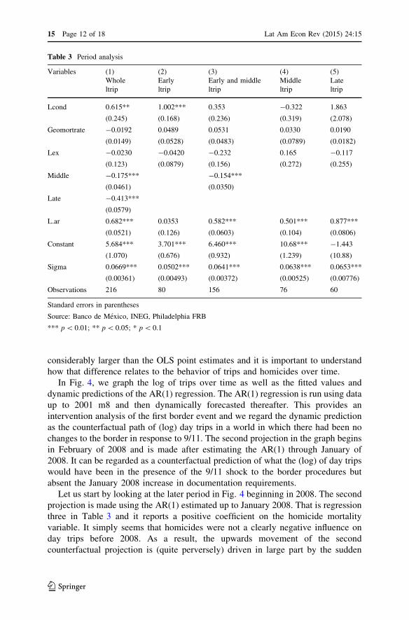
Table 3 presents AR(1) estimates of the determinants of day trips using the same

three specifications of homicide mortality as we examined using OLS/Newey–West.

The results are quite unlike OLS in that only when homicides are entered as a rate

do they have a negative influence on day trips. The exchange rate also has an

unexpectedly positive sign in the other formulations. In contrast, the point estimates

for the effect of the two border changes are relatively stable: the 2001 change

reduced trips by 18–20 % and the 2008 change by 42–49 %. These effects are

18 The US Census department’s X11 and X12 are popular examples for automatically fitting ARIMA

models, but a variety of approaches have been explored (Hoglund and Ostermark 1991; Melard and

Pasteels 2000).

Lat Am Econ Rev (2015) 24:15 Page 11 of 18 15

123

considerably larger than the OLS point estimates and it is important to understand

how that difference relates to the behavior of trips and homicides over time.

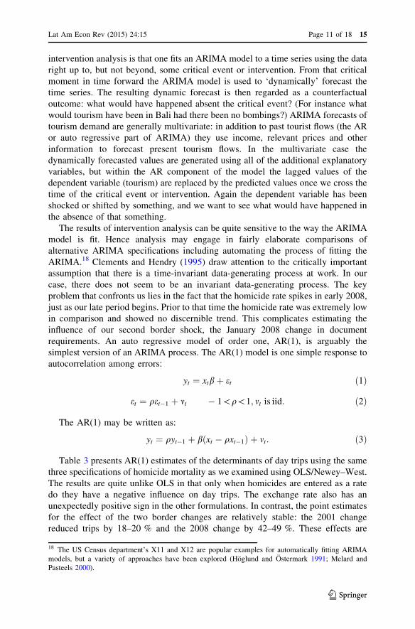
In Fig. 4, we graph the log of trips over time as well as the fitted values and

dynamic predictions of the AR(1) regression. The AR(1) regression is run using data

up to 2001 m8 and then dynamically forecasted thereafter. This provides an

intervention analysis of the first border event and we regard the dynamic prediction

as the counterfactual path of (log) day trips in a world in which there had been no

changes to the border in response to 9/11. The second projection in the graph begins

in February of 2008 and is made after estimating the AR(1) through January of

2008. It can be regarded as a counterfactual prediction of what the (log) of day trips

would have been in the presence of the 9/11 shock to the border procedures but

absent the January 2008 increase in documentation requirements.

Let us start by looking at the later period in Fig. 4 beginning in 2008. The second

projection is made using the AR(1) estimated up to January 2008. That is regression

three in Table 3 and it reports a positive coefficient on the homicide mortality

variable. It simply seems that homicides were not a clearly negative influence on

day trips before 2008. As a result, the upwards movement of the second

counterfactual projection is (quite perversely) driven in large part by the sudden

Table 3 Period analysis

Variables (1) (2) (3) (4) (5)

Whole Early Early and middle Middle Late

ltrip ltrip ltrip ltrip ltrip

Lcond 0.615** 1.002*** 0.353 -0.322 1.863

(0.245) (0.168) (0.236) (0.319) (2.078)

Geomortrate -0.0192 0.0489 0.0531 0.0330 0.0190

(0.0149) (0.0528) (0.0483) (0.0789) (0.0182)

Lex -0.0230 -0.0420 -0.232 0.165 -0.117

(0.123) (0.0879) (0.156) (0.272) (0.255)

Middle -0.175*** -0.154***

(0.0461) (0.0350)

Late -0.413***

(0.0579)

L.ar 0.682*** 0.0353 0.582*** 0.501*** 0.877***

(0.0521) (0.126) (0.0603) (0.104) (0.0806)

Constant 5.684*** 3.701*** 6.460*** 10.68*** -1.443

(1.070) (0.676) (0.932) (1.239) (10.88)

Sigma 0.0669*** 0.0502*** 0.0641*** 0.0638*** 0.0653***

(0.00361) (0.00493) (0.00372) (0.00525) (0.00776)

Observations 216 80 156 76 60

Standard errors in parentheses

Source: Banco de Mexico, INEG, Philadelphia FRB

*** p\ 0.01; ** p\ 0.05; * p\ 0.1

15 Page 12 of 18 Lat Am Econ Rev (2015) 24:15

123

spike in homicides in 2008 and after.19 Table 3 presents the estimates of the

homicide rate formulation of the AR(1) for different time periods. We see the early,

middle and late periods separately. The data from the early period is used to

estimate the coefficients for the model that produces the first dynamic forecast,

while the data from both the early and middle period is used to estimate the

coefficients used to produce the second dynamic forecast. In both cases the

coefficients on mortality are positive, so that when mortality suddenly increases in

2008 this causes the dynamically prediction to perversely rise rather than fall.20

To visualize the size of the problem at hand we have graphed a very simple

adjustment to the second projection. This is the short dashed line that begins in the

same place as the second projection but lies below it. We have subtracted from the

second projection the perverse positive effect of homicides and we have also

appealed to the AR(1) regression for the whole span of data (regression one) to tell

us how much we should further lower the projection to account for the negative

effect of homicides in the late period.21 So the dashed line is simply the projection

less (0.0531 ? 0.0192)*geomortalityrate: the first term removes the perversely

positive influence of homicides and the second accounts for the negative influence

of homicides using the parameter from the full period AR(1). Visually this

downwards adjustment of the late period projection is quite significant. It seems to

Fig. 4 Log trips to Mexico and projections. Source: Banco de Mexico, INEG, Philadelphia FRB

19 Note that only the AR(1) for the whole period reports a negative coefficient on homicides. Not even

the AR(1) for the late period does—the negative influence of homicides is only revealed when we look

across the periods.20 We also see substantial changes to our coefficients over the various sub periods. This suggests that we

do not have an unchanging data-generating process.21 We could have appealed to the Prais regression in Table Two, which reports a very similar coefficient

on homicides, but we prefer to bias the results against the hypothesis that the border changes have

significantly reduced day trips.

Lat Am Econ Rev (2015) 24:15 Page 13 of 18 15

123

roughly halve the yawning gap between the projection and the number of actual

trips.

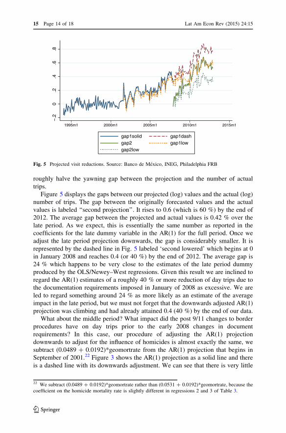
Figure 5 displays the gaps between our projected (log) values and the actual (log)

number of trips. The gap between the originally forecasted values and the actual

values is labeled ‘‘second projection’’. It rises to 0.6 (which is 60 %) by the end of

2012. The average gap between the projected and actual values is 0.42 % over the

late period. As we expect, this is essentially the same number as reported in the

coefficients for the late dummy variable in the AR(1) for the full period. Once we

adjust the late period projection downwards, the gap is considerably smaller. It is

represented by the dashed line in Fig. 5 labeled ‘second lowered’ which begins at 0

in January 2008 and reaches 0.4 (or 40 %) by the end of 2012. The average gap is

24 % which happens to be very close to the estimates of the late period dummy

produced by the OLS/Newey–West regressions. Given this result we are inclined to

regard the AR(1) estimates of a roughly 40 % or more reduction of day trips due to

the documentation requirements imposed in January of 2008 as excessive. We are

led to regard something around 24 % as more likely as an estimate of the average

impact in the late period, but we must not forget that the downwards adjusted AR(1)

projection was climbing and had already attained 0.4 (40 %) by the end of our data.

What about the middle period? What impact did the post 9/11 changes to border

procedures have on day trips prior to the early 2008 changes in document

requirements? In this case, our procedure of adjusting the AR(1) projection

downwards to adjust for the influence of homicides is almost exactly the same, we

subtract (0.0489 ? 0.0192)*geomortrate from the AR(1) projection that begins in

September of 2001.22 Figure 3 shows the AR(1) projection as a solid line and there

is a dashed line with its downwards adjustment. We can see that there is very little

−.2

0.2

.4.6

.8

2015m11995m1 2010m12005m12000m1

gap1solid gap1dashgap2 gap1lowgap2low

Fig. 5 Projected visit reductions. Source: Banco de Mexico, INEG, Philadelphia FRB

22 We subtract (0.0489 ? 0.0192)*geomortrate rather than (0.0531 ? 0.0192)*geomortrate, because the

coefficient on the homicide mortality rate is slightly different in regressions 2 and 3 of Table 3.

15 Page 14 of 18 Lat Am Econ Rev (2015) 24:15

123

downwards adjustment prior to 2008. That is simply because the homicide rate is

very low until 2008. In this case the unadjusted gap between the (log of the)

projected values and the (log of the) actual number of day trips is 0.21 (21 %) and

the adjusted is 0.17 (17 %). These are averages over the middle period but by

December 2007 it had risen to 0.26 (26 %).

6 Conclusions

We have found that the flow of short-term visits over the US–Mexico border was

significantly reduced by the changes to border procedures set in train by 9/11. Our

findings add to the literature on the importance of border documents and visas for

tourism flows. The reductions in border tourism and day trips were clearly of

tremendous importance for the Mexican border economy and particularly for its

tourism and retail sector. The potential size of the reduction in spending is quite

large. As it is the Secretarıa de Turismo (2014) estimates that total spending by

persons on day trips (Excursionistas internacionales sin pernocta) was 1.53 billion

USD in 2012. How much larger might that figure have been had there been no

border changes?

The AR(1) time series estimates are consistent with the OLS regression’s 24 %

estimated reduction in day trips after the second of the two border changes (January

2008). The average gap between the AR(1) forecasted path of day trips and the

actual path of day trips is also 24 %, but only once we adjust the forecast

downwards to better account for the sudden rise of homicides after 2008. Of course

averages contain variations over time and that gap was estimated to be quite a bit

larger by 2012 than it started in 2008—it had become a nearly 40 % gap. Even

larger gaps appear in Fig. 5 when we forecasted day trips beginning back in 2001

rather than 2008. The average gap between our (downwards adjusted) first

prediction and the actual number of day trips was 47 % after 2008, but again the gap

was rising and became 60 % by 2012. These are really very large effects so it is

worth recalling that day trips fell some 20 % from 2000 to 2012 while international

tourism to the interior of Mexico rose some 40 %. So the notion that day trips (and

associated spending) might have been 60 % higher had there been no changes to

border procedures should not be regarded as inherently implausible.23 Growth of

60 % would still have paled in comparison to the sixfold increase in the value of

international trade across the same period.

We do not think that the data at our disposal is well suited to examining whether

and how changes in day trips and legitimate commerce affected homicides and the

drugs wars in Mexico. But it is difficult to see how the reduction in legitimate

commerce associated with the contraction of day trips could have helped the

situation. To our minds the natural assumption is that the contraction in legitimate

commerce exacerbated the problem. To the extent that this is true we underestimate

23 A recent study of the effect of more stringent security measures at the US–Canadian border (Lipovic

et al. 2015) found the flow of American day-trippers to Canada had been reduced by 59 %, while

Canadian day trips to the US had been curtailed by 50 %.

Lat Am Econ Rev (2015) 24:15 Page 15 of 18 15

123

the negative influence of the border restrictions. But we think that considerable

geographic and political detail would be needed to evaluate the issue with any

success.24

We have tried to respond responsibly to the estimation problems created by the

fact that homicides in Mexico rose quickly on the heels of our second change in

border procedures. It would certainly be better to have information at the household

level on the number of trips made to specific places in Mexico along with

demographic and economic characteristics. Ideally this would be matched with

survey information that reported something about their typical motivations for

crossing the border as well as their level of concern about violence over the border.

But even with only highly aggregated information we have been able to conclude

that changes in US border procedures have had a large and enduringly negative

impact on tourism and travel on the Mexican border, one that has clearly been

economically and socially meaningful. The wider message for the tourism and

hospitality industry is that changes to border procedures bear very close attention.

6.1 Data sources

1. Banco de Mexico. Day Trips (Excursionistas Fronterizos) REPORTE DE

FLUJOS TURISTICOS A MEXICO—REPORTE MENSUAL http://www.

siimt.com/en/siimt/siim_flujos_mensuales

2. Philadelphia FRB Monthly coincident index for each of the 50 states. http://

www.philadelphiafed.org/research-and-data/regional-economy/indexes/

coincident/

3. Intituto Nacional De Estadistica Y Geografa, Sistema Estatal y Municipal de

Bases de Datos (SIMBAD), Homicide rates by state Defunciones por homicidio

http://sc.inegi.org.mx/sistemas/cobdem/resultados.jsp?w=18&Backidhecho=

18&Backconstem=17&constembd=208

Results produced by STATA do file: LAERfinal1.

Acknowledgments We thank Richard Spady for his exceptionally generous provision of advice and

assistance. Jin Man Lee provided very helpful comments. Julian Lambert and Amy Lewis provided able

research assistance. We would also like to thank Daniela Leaman of the Mexico Tourism Board, Chicago,

for bringing the data on Mexican tourist flows to our attention.

Open Access This article is distributed under the terms of the Creative Commons Attribution 4.0

International License (http://creativecommons.org/licenses/by/4.0/), which permits unrestricted use, dis-

tribution, and reproduction in any medium, provided you give appropriate credit to the original

author(s) and the source, provide a link to the Creative Commons license, and indicate if changes were

made.

24 Luke Chicoine’s (2015) recent work on how local political instability interacted with an influx of high-

powered weapons from the US to raise the homicide rate is an excellent example.

15 Page 16 of 18 Lat Am Econ Rev (2015) 24:15

123

References

Andreas P (2003) A tale of two borders: the U.S.-Mexico and U.S.-Canada lines after 9/11. Center for

comparative immigration studies. Center for Comparative Immigration Studies, UC San Diego.

Retrieved from: http://escholarship.org/uc/item/6d09j0n2

Blanke J, Chiesa T (2013) The travel and tourism competitiveness report 2013. World Economic Forum.

Retreived from http://www.weforum.org/reports/travel-tourism-competitiveness-report-2013

Box GE, Jenkins GM (1970) Time series. Forecasting and control. Holden-Day, San Francisco

Box GE, Jenkins GM (1976) Time series analysis: forecasting and control. Holden-Day, San Francisco

Box GE, Tiao GC (1975) Intervention analysis with applications to economic and environmental

problems. J Am Stat Assoc 70(349):70–79

Bringas Rabago N (2005) Turismo fronterizo: un estudio de caso. In: Vicente FL, Guzman TJL-G (eds),

Turismo sostenible : un enfoque multidisciplinar e internacional. Cordoba, Universidad de Cordoba,

pp 179–216. Retrieved from http://dialnet.unirioja.es/servlet/libro?codigo=9162

Brohman J (1996) New directions in tourism for third world development. Ann Tour Res 23(1):48–70

Canally C, Timothy DJ (2007) Perceived constraints to travel across the US-Mexico border among

American university students. Int J of Tour Res 9(6):423–437

Chicoine LE (2015) Homicides in Mexico and the expiration of the U.S. Federal assault weapons ban: a

difference-in-discontinuities approach. Retrieved from http://sites.google.com/site/lukechicoine/

research

Chu F-L (1998) Forecasting tourism: a combined approach. Tour Manag 19(6):515–520

Clancy MJ (1999) Tourism and development evidence from Mexico. Ann Tour Res 26(1):1–20

Clements MP, Hendry DF (1995) Macro-economic forecasting and modelling. Econ J

105(431):1001–1013

Commerce WCO (2014) Passport information for entering Mexico. Retrieved from http://www.weslaco.

com/visitors/passport

Cooper A, Rumford C (2013) Monumentalising the border: bordering through connectivity. Mobilities

8(1):107–124

Coronado RA, Phillips KR (2012) Spotlight: dollar-sensitive Mexican shoppers boost Texas border retail

activity. Southw Econ (Q4). Retreived from http://www.dallasfed.org/assets/documents/research/

swe/2012/swe1204g.pdf

David L, Toth G, Bujdoso Z, Remenyik B (2011) The role of tourism in the development of border

regions in Hungary. Revista Romana de Economie 33(2):42

Enders W, Sandler T, Parise GF (1992) An econometric analysis of the impact of terrorism on tourism.

Kyklos 45(4):531–554

Garvey Schubert Barer Law (2007) Important change in travel documentation required for travel to U.S.

from Canada or Mexico. Retreived from https://www.gsblaw.com/news/legal_update/important_

change_in_travel_documentation_required_for_travel_to_us_from_canada_or_mexico/

Goh C, Law R (2002) Modeling and forecasting tourism demand for arrivals with stochastic nonstationary

seasonality and intervention. Tour Manag 23(5):499–510

Hampton MP (2010) Enclaves and ethnic ties: the local impacts of Singaporean cross-border tourism in

Malaysia and Indonesia. Singap J Trop Geogr 31(2):239–253

Helfenstein U (1991) The use of transfer function models, intervention analysis and related time series

methods in epidemiology. Int J Epidemiol 20(3):808–815

Hoglund R, Ostermark R (1991) Automatic ARIMA modelling by the cartesian search algorithm.

J Forecast 10(5):465–476

Imhoff M, Bauer M, Gather U, Lohlein D (1998) Time series analysis in intensive care medicine:

technical Report, SFB 475: Komplexitatsreduktion in Multivariaten Datenstrukturen, Universitat

Dortmund. Retrieved from http://hdl.handle.net/10419/77286

Ismail Z, Yahaya A, Efendi R (2009) Intervention model for analyzing the impact of terrorism to tourism

industry. J Math Stat 5(4):322

Jensen L (1990) Guidelines for the application of ARIMA models in time series. Res Nurs Health

13(6):429–435

Kulendran N, Witt SF (2003) Forecasting the demand for international business tourism. J Travel Res

41(3):265–271

Lat Am Econ Rev (2015) 24:15 Page 17 of 18 15

123

Lagiewski RM, Revelas DA (2004) Challenges in cross-border tourism regions. In: Annual Conference of

the European Council of Hotel, Restaurant and Institutional Educators. Ankara, Turkey. Retreived

from http://scholarworks.rit.edu/other/551/

Lahrech A, Sylwester K (2013) The impact of NAFTA on North American stock market linkages. N Am J

Econ Fin 25:94–108

Lee C-K, Song H-J, Bendle LJ (2010a) The impact of visa-free entry on outbound tourism: a case study of

South Korean travellers visiting Japan. Tour Geogr 12(2):302–323

Lee MH, Suhartono S, Sanugi B (2010b) Multi input intervention model for evaluating the impact of the

Asian crisis and terrorist attacks on tourist arrivals. Matematika 26(1):83–106

Lipovic L, Sido M, Ghoshal A (2015) Integration interrupted: the impact of September 11, 2001. J Econ

Integr 30(1):66–92

Mann S (2005) Development through tourism: the World Bank’s Role. World Bank, Washington

Martinez OJ (1994) The dynamics of border interaction. Glob Bound World Bound 1:1–15

Melard G, Pasteels J-M (2000) Automatic ARIMA modeling including interventions, using time series

expert software. Int J Forecast 16(4):497–508

Philadelphia FRB (2015) State Coincident Indexes. Retrieved from https://www.philadelphiafed.org/

research-and-data

Prokkola E-K (2010) Borders in tourism: the transformation of the Swedish–Finnish border landscape.

Curr Issue Tour 13(3):223–238

Rodriguez O (2014) Mexico’s border cities hope to lure back U.S. tourists. Seattle Times. Retrieved from

http://seattletimes.com/html/travel/2023098630_mexicoborderspringbreakxml.html

Secretarıa de Turismo-REDES Sociedad Civil (1996) Importancia economica del turismopara Baja

California. SECTUR-REDES Sociedad civil, Mexico

Sharpley R, Telfer DJ (2002) Tourism and development: concepts and issues (Vol. 5): Channel View

Publications, Clevedon

Sirakaya E, Sheppard AG, McLellan RW (1997) Assessment of the relationship between perceived safety

at a vacation site and destination choice decisions: extending the behavioral decision-making model.

J Hosp Tour Res 21(2):1–10. doi:10.1177/109634809702100201

Song H, Li G (2008) Tourism demand modelling and forecasting—a review of recent research. Tour

Manag 29(2):203–220

Stock JH, Watson MW (1989) New indexes of coincident and leading economic indicators. In: Blanchard

OJ, Fischer S (eds) NBER Macroeconomics Annual 1989, vol 4. MIT Press, pp 351–409

Stronge WB, Redman M (1982) US tourism in Mexico: an empirical analysis. Ann Tour Res 9(1):21–35

Thomson A (2008) Mexico-US frontier culture roughly sundered. Financial Times. Retrieved from http://

on.ft.com/1wxQHUP

Transactional Records Access Clearinghouse SU (2006) Border patrol agents: southern versus northern

border. Retrieved 26 Jan 2015 from, http://trac.syr.edu/immigration/reports/143/include/

rep143table2.html

Turismo SD (2014) Resultados de la Actividad Turıstica, enero—diciembre 2013, from http://consulmex.

sre.gob.mx/montreal/images/Consulado/Comunicado/rat2013_18feb14.pdf

Wilson C, Lee E (2013) The state of the border report: a comprehensive analysis of the US-Mexico

Border. Washington, DC: Wilson Center. Retrieved from http://www.wilsoncenter.org/sites/default/

files/mexico_state_of_border_0.pdf

15 Page 18 of 18 Lat Am Econ Rev (2015) 24:15

123