Use of Cellular Automata-Based Arti�cial NeuralNetworks For Detection and Prediction of Land UseChanges in North Eastern Dhaka CityFoyezur Rahman 

Military Institute of Science and TechnologyMd. Tauhid Ur Rahman  ( tauhid_cee@yahoo.com )

Military Institute of Science and Technology

Research Article

Keywords: Urbanization, LST, UHI, NDVI, NDBI, CA-ANN

Posted Date: November 15th, 2021

DOI: https://doi.org/10.21203/rs.3.rs-993126/v1

License: This work is licensed under a Creative Commons Attribution 4.0 International License.  Read Full License

1

Use of Cellular Automata-based Artificial Neural Networks for Detection and 1

Prediction of Land Use Changes in North Eastern Dhaka City 2

3

Foyezur Rahman 4

Professor, Department of Civil Engineering, Military Institute of Science and Technology 5

(MIST), Dhaka-1216, Bangladesh 6

Md. Tauhid Ur Rahman* 7

Professor, Department of Civil Engineering, Military Institute of Science and Technology 8

(MIST), Dhaka-1216, Bangladesh 9

10

*Corresponding Author: 11

tauhid_cee@yahoo.com 12 Department of Civil Engineering, Military Institute of Science and Technology 13 Phone: +880 1965-965956 14

2

Abstract 15

The purpose of this study was to examine the pattern of change in Land Use Land Cover 16

(LULC) and Land Surface Temperature (LST) in Mirpur and its surrounding area (north-17

eastern part of Dhaka) over the last 30 years using Landsat Satellite images and remote 18

sensing indices, and to develop relationships between LULC types and LST, as well as to 19

analyze their impact on local warming. Using this analyzed data, a further projection of 20

LULC and LST change over the next two decades was made. From 1989 to 2019, five-year 21

intervals of Landsat 4-5 TM and Landsat 8 OLI pictures were utilized to track the 22

relationship between LULC changes and LST. Cellular Automata-based Artificial Neural 23

Network (CA-ANN) algorithm was used to model the LULC and LST maps for the year 24

2039. Two environmental indices were analyzed to determine their link with LST: the 25

Normalized Difference Vegetation Index (NDVI) and the Normalized Difference Built-up 26

Index (NDBI). The link between LST and LULC types indicates that built-up area raises 27

LST by substituting non-evaporating surfaces for natural vegetation. The average surface 28

temperature has been increasing steadily for the previous 30 years. For the year 2019, it was 29

determined that roughly 86 percent of total land area has been converted to built-up area and 30

that 89 percent of land area has an LST greater than 28°C. According to the study, if the 31

current trend continues, 72 percent of the Mirpur area is predicted to see temperatures near 32

32°C in 2039. Additionally, LST had a significant positive association with NDBI and a 33

negative correlation with NDVI. The overall accuracy of LULC was greater than 90%, with 34

a Kappa coefficient of 0.83. The study may assist urban planners and environmental 35

engineers in comprehending and recommending effective policy measures and plans to 36

mitigate the consequences of LULC. 37

Keywords: Urbanization, LST, UHI, NDVI, NDBI, CA-ANN 38

3

1. Introduction 39

Bangladesh is one of the heavily populated countries in South Asia, and over the past century, it 40

has also experienced rapid population growth. The explosion of population growth mainly took 41

place in the City areas. It is estimated that almost all other men, women, and children will be living 42

in urban areas in the future (M. Rahman, A. S. Aldosary, & M. Mortoja, 2017). Dhaka, the capital 43

of Bangladesh, is one of the world's fastest expanding megacities (M. Rahman, A. S. Aldosary, & 44

M. Mortoja, 2017; Dewan & Yamaguchi, 2009; Meyer & Turner, 1992). Thus, while rising 45

urbanization in Dhaka is likely to have a significant impact on land cover changes and, 46

subsequently, on the urban microclimate, little is known about these developments. Additionally, 47

it is home to almost 16 million people and covers an area of around 304.16 square kilometers. This 48

city's population has expanded by nearly 11 million people during the last two decades (Dewan & 49

Yamaguchi, 2009). Dhaka is spreading vertically and horizontally as a result of this population 50

explosion driven primarily by rural-urban migration and partially by natural growth, and these 51

expansions have been highlighted as a major contributor to the increase in Land Surface 52

Temperature (LST) (Al-sharif & Pradhan, 2014). 53

Urbanization refers to the process of the change of country area to a City area, which is the result 54

of population immigration, administrative services, construction of new infrastructure, and 55

development of industry and service sector. Over the past few years, the Land Use Land Cover 56

(LULC) change mechanism at the national and local level has also drawn the attention of 57

researchers. It is reported that LULC's global spatial dynamics also reveal the connection between 58

land-use change and human activity (Corner, Dewan, & Chakma, 2014; Dewan & Yamaguchi, 59

2009; Meyer & Turner, 1992; M. S. Rahman, Mohiuddin, Kafy, Sheel, & Di, 2018). Some scholars 60

emphasized the effects on LULC changes by urbanization, believing that population growth and 61

economic development contributed to urban expansion and a large number of water and 62

agricultural land transformations into built-up areas. This transition also affects the local, regional 63

and global ecosystems, including habitat quality, green areas, and destruction of the environment 64

(Dewan, Kabir, Nahar, & Rahman, 2012; Dewan & Yamaguchi, 2009; IPCC, 2014; Lilly Rose, 65

2009). The mechanism of LULC transition is complex as the relationship depends on different 66

scales of natural and socio-economic factors (Chen, Zhao, Li, & Yin, 2006; McKinney, 2002; Tran 67

et al., 2017). The associated factors have an impact on the change in LULC due to the scale effect 68

4

and vulnerability of the land system dynamics and it is, therefore, vital to understand its relation. 69

Meanwhile, accurate prediction for future land use is essentially required to avoid unexpected 70

urbanization, which is necessary to plan and manage land use (Ahmed, 2011a; Balogun & Ishola, 71

2017; M. Rahman et al., 2017; M. S. Rahman et al., 2018). 72

Human migration to Cities causes urban areas to grow every year and creates rapid changes to 73

their ecosystems, biodiversity, natural landscapes, and the environment (McKinney, 2002). More 74

than 70% of the world's population is anticipated to live in urban areas in the next 30 years (Celik, 75

Kaya, Alganci, & Seker, 2019; Grimmond, 2007; Handayanto, Kim, & Tripathi, 2017; Kafy, 76

Islam, Ferdous, Khan, & Hossain, 2019; M. Rahman et al., 2017; Ullah et al., 2019). While this 77

development is a sign of economic growth and economic stability in the region, it has several short 78

and long-term consequences. Over the last decade, geographers, urban planners, and climate 79

scientists have been paying considerable attention to elevated LST over urban areas (Al-sharif & 80

Pradhan, 2014; Kafy et al., 2019; Maduako, Yun, & Patrick, 2016; M. Rahman, 2016; Zheng, 81

Shen, Wang, & Hong, 2015; Zine El Abidine, Mohieldeen, Mohamed, Modawi, & Al-Sulaiti, 82

2014). Several studies suggest that population expansion appears to increase the average LST in 83

urban environments by 2-4°C in contrast with rural areas (Maimaitiyiming et al., 2014; Mozumder 84

& Tripathi, 2014; Thapa & Murayama, 2009; Yu, Guo, & Wu, 2014). Increased LSTs and Urban 85

Heat Island (UHI) impact have been associated with high energy consumption, air pollution, and 86

health issues, including the deaths of children and elders from asthma and heat stroke (Ahmed, 87

Kamruzzaman, Zhu, Rahman, & Choi, 2013; Maduako et al., 2016; M. T. Rahman, A. S. Aldosary, 88

& M. Mortoja, 2017; M. T. Rahman & Rashed, 2015; Scarano & Sobrino, 2015; Zhi-hao, Wen-89

juan, Ming-hua, Karnieli, & Berliner, 2011; Zhou, Huang, & Cadenasso, 2011). 90

Bangladesh is one among the world's most populous countries, according to the "Bangladesh Delta 91

Plan 2100." The overall population density, according to 2011 census statistics, is around 1,015 92

persons per square kilometer. Recent UN figures indicate that roughly 25% of Bangladesh's current 93

population resides in urban areas. More than half of this urban population resides in four major 94

cities: Dhaka, Chittagong, Khulna, and Rajshahi. The population density is currently estimated to 95

be over 34,000 people per square kilometer, placing Dhaka among the world's most densely 96

inhabited cities. In 1976, the rural settlement area was projected to be 885,637 hectares, accounting 97

for 6.1 percent of the total land area of the nation. Rural settlement area rose at a quicker pace over 98

5

time, reaching 10% (1,458,031 ha) in 2000 and 12.1 percent (1,766,123 ha) in 2010. (van 99

Scheltinga, Quadir, & Ludwig, 2015). 100

Examining LULC change in the last few decades has become an increasing concern because of 101

biodiversity decreasing, habitat changing, and altering the regional and global climate patterns and 102

composition (J. Li & Zhao, 2003; Lilly Rose, 2009; Mishra & Rai, 2016). It can be challenging, 103

complicated, and likely to yield contradictory results to detect and tests changes in LULC through 104

direct field visits (Meyer & Turner, 1992; M. Rahman, 2016; Zheng et al., 2015). Over the past 105

few decades, developments and integration of Remote Sensing and Geographic Information 106

System (GIS) technologies have overcome most of the constraints and are now powerful methods 107

for assessing, monitoring changes in LST and LULCs (Corner et al., 2014; Fu & Weng, 2018; Hart 108

& Sailor, 2009; Islam & Ahmed, 2011). Even since the early 1970s, the use of remote sensing 109

techniques to measure LSTs and investigate the development and spatial distribution of UHIs has 110

been quite successful. Research has identified that massive changes of various LULC components 111

(water bodies, vegetation, and agricultural lands) contribute to the increase in LST which 112

significantly stimulus the generation of UHI effect (Bahi, Rhinane, Bensalmia, Fehrenbach, & 113

Scherer, 2016; Lambin, 1999; Maduako et al., 2016). LST is recognized as one of the main factors 114

for urban microclimate warming. Several local issues are closely linked to the LST, such as 115

biophysical hazards (e.g. heat stress), air pollution, and public health concerns (Amiri, Weng, 116

Alimohammadi, & Alavipanah, 2009; Chander, Markham, & Helder, 2009; Gutman, Huang, 117

Chander, Noojipady, & Masek, 2013; Streutker, 2003). As the rise in surface temperature 118

contributes significantly to the deterioration of the ecological balance, it is, therefore, important to 119

obtain LST as a first and primary step and then to model possible LST so that policies can be 120

implemented to mitigate the negative environmental impacts (Celik et al., 2019; M. Rahman et al., 121

2017; M. T. Rahman et al., 2017; M. T. Rahman & Rashed, 2015; Shatnawi & Abu Qdais, 2019; 122

Weng, Lu, & Schubring, 2004). 123

As LST is largely dependent on LULC therefore, prediction of LULC for evaluating future change 124

in LST is needed. Cellular Automata-Artificial Neural Network (CA-ANN) model provides a solid 125

understanding of the complexities of the spatial system to evaluate and predict LULC changing 126

patterns. To monitor previous and existing LULC and determine the potential impacts of LULC 127

on the city area, this study mainly focuses on predicting future changes of LULC and identifies its 128

6

impacts on future LST. Using a CA-ANN model, the simulation of future land cover can be 129

analysed. The CA-ANN model, together with the geographical information system, is widely 130

regarded as the most powerful tool for modelling the probabilities of the spatiotemporal shift in 131

LULC (Arsanjani, Helbich, Kainz, & Boloorani, 2013; Santé, García, Miranda, & Crecente, 2010). 132

Under these circumstances stated above, the research is primarily planned to investigate LULC 133

and LST shifts in the past two decades (1989-2019) through the use of recent and historically 134

archived Landsat satellite images in Mirpur and its surrounding area. Also, a simulation will be 135

done by using ANN-based CA algorithm to predict the future growth and surface temperature of 136

the Mirpur and its surrounding area for the year 2039. 137

138

7

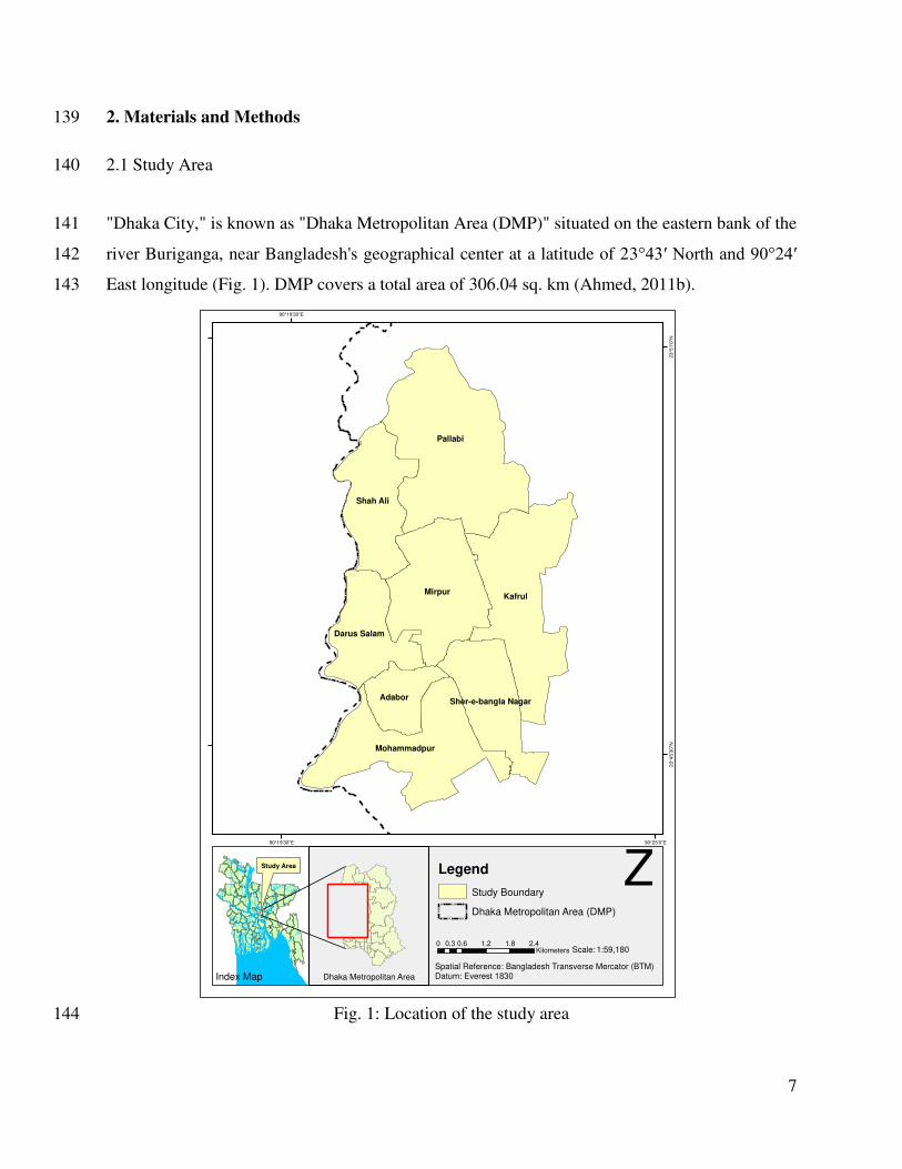
2. Materials and Methods 139

2.1 Study Area 140

"Dhaka City," is known as "Dhaka Metropolitan Area (DMP)" situated on the eastern bank of the 141

river Buriganga, near Bangladesh's geographical center at a latitude of 23°43′ North and 90°24′ 142

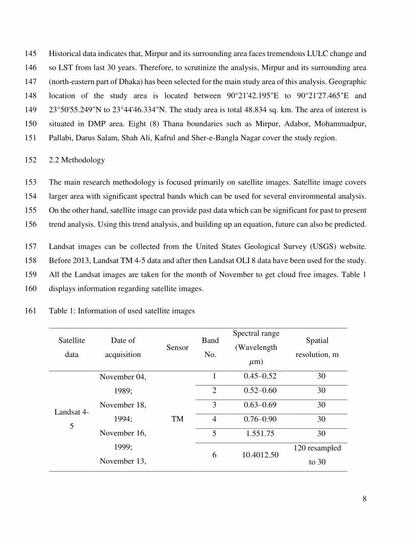
East longitude (Fig. 1). DMP covers a total area of 306.04 sq. km (Ahmed, 2011b). 143

Fig. 1: Location of the study area 144

Scale:

Spatial Reference: Bangladesh Transverse Mercator (BTM)Datum: Everest 1830Index Map

Pallabi

KafrulMirpur

Shah Ali

Mohammadpur

Darus Salam

AdaborSher-e-bangla Nagar

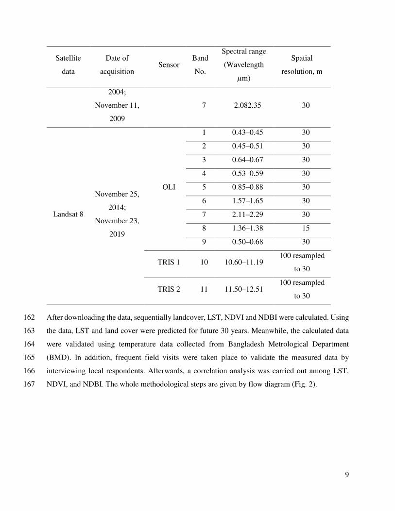
90°19'30"E

90°19'30"E

90°25'0"E

23

°51

'0"N

23

°45

'30

"N

0 0.6 1.2 1.8 2.40.3Kilometers 1:59,180

Legend

Study Boundary

Dhaka Metropolitan Area (DMP)

ZStudy Area

Dhaka Metropolitan Area

8

Historical data indicates that, Mirpur and its surrounding area faces tremendous LULC change and 145

so LST from last 30 years. Therefore, to scrutinize the analysis, Mirpur and its surrounding area 146

(north-eastern part of Dhaka) has been selected for the main study area of this analysis. Geographic 147

location of the study area is located between 90°21'42.195"E to 90°21'27.465"E and 148

23°50'55.249"N to 23°44'46.334"N. The study area is total 48.834 sq. km. The area of interest is 149

situated in DMP area. Eight (8) Thana boundaries such as Mirpur, Adabor, Mohammadpur, 150

Pallabi, Darus Salam, Shah Ali, Kafrul and Sher-e-Bangla Nagar cover the study region. 151

2.2 Methodology 152

The main research methodology is focused primarily on satellite images. Satellite image covers 153

larger area with significant spectral bands which can be used for several environmental analysis. 154

On the other hand, satellite image can provide past data which can be significant for past to present 155

trend analysis. Using this trend analysis, and building up an equation, future can also be predicted. 156

Landsat images can be collected from the United States Geological Survey (USGS) website. 157

Before 2013, Landsat TM 4-5 data and after then Landsat OLI 8 data have been used for the study. 158

All the Landsat images are taken for the month of November to get cloud free images. Table 1 159

displays information regarding satellite images. 160

Table 1: Information of used satellite images 161

Satellite

data

Date of

acquisition Sensor

Band

No.

Spectral range

(Wavelength 𝜇m)

Spatial

resolution, m

Landsat 4-

5

November 04,

1989;

November 18,

1994;

November 16,

1999;

November 13,

TM

1 0.45–0.52 30

2 0.52–0.60 30

3 0.63–0.69 30

4 0.76–0.90 30

5 1.551.75 30

6 10.4012.50 120 resampled

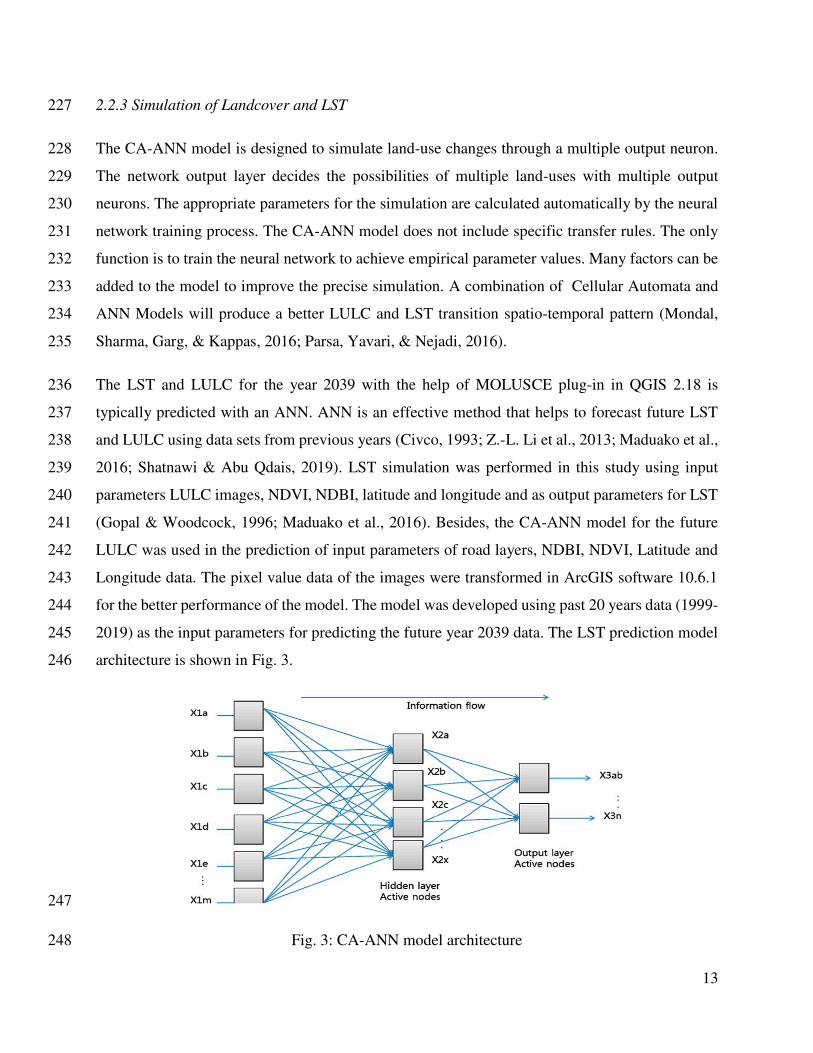
to 30

9

Satellite

data

Date of

acquisition Sensor

Band

No.

Spectral range

(Wavelength 𝜇m)

Spatial

resolution, m

2004;

November 11,

2009

7 2.082.35 30

Landsat 8

November 25,

2014;

November 23,

2019

OLI

1 0.43–0.45 30

2 0.45–0.51 30

3 0.64–0.67 30

4 0.53–0.59 30

5 0.85–0.88 30

6 1.57–1.65 30

7 2.11–2.29 30

8 1.36–1.38 15

9 0.50–0.68 30

TRIS 1 10 10.60–11.19 100 resampled

to 30

TRIS 2 11 11.50–12.51 100 resampled

to 30

After downloading the data, sequentially landcover, LST, NDVI and NDBI were calculated. Using 162

the data, LST and land cover were predicted for future 30 years. Meanwhile, the calculated data 163

were validated using temperature data collected from Bangladesh Metrological Department 164

(BMD). In addition, frequent field visits were taken place to validate the measured data by 165

interviewing local respondents. Afterwards, a correlation analysis was carried out among LST, 166

NDVI, and NDBI. The whole methodological steps are given by flow diagram (Fig. 2). 167

10

168

Fig. 2: Methodological flow diagram of the study 169

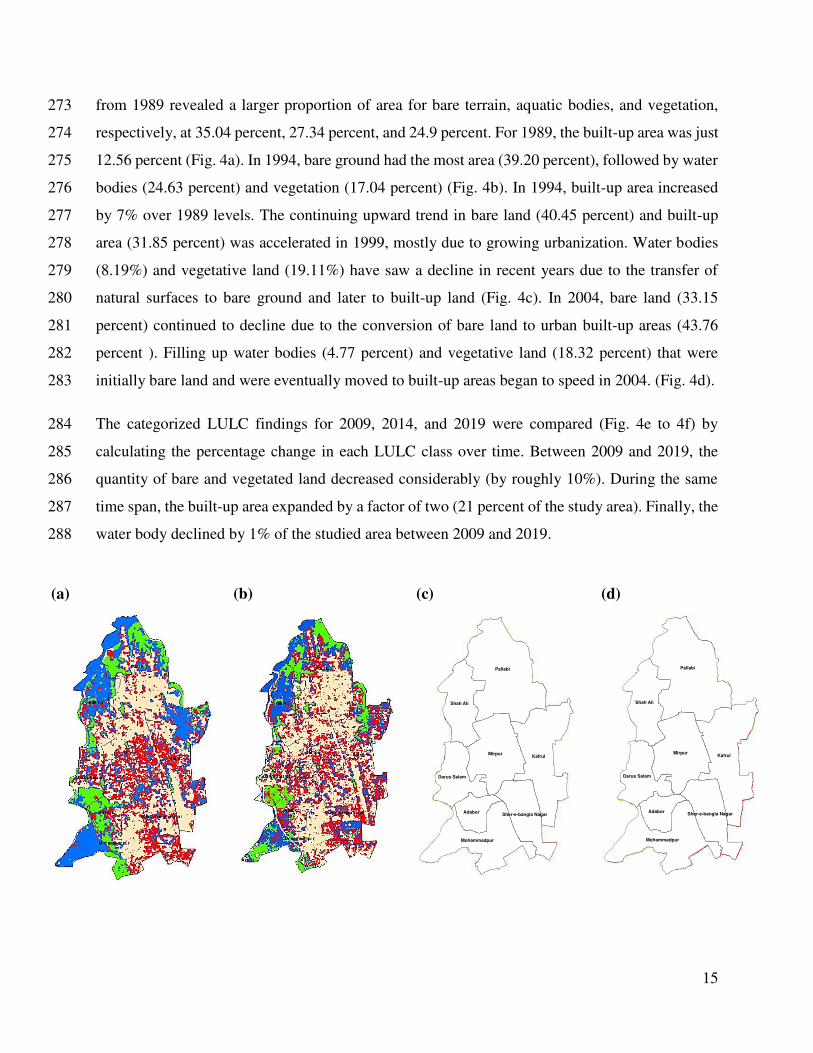
2.2.1 Land Use Land Cover Classification 170

ArcGIS 10.6.1 software was used to combine the satellite images obtained. To choose training 171

samples and identify the various LULC classes, a True Color Composite (TCC) was created using 172

appropriate band combinations for all images (d'Entremont & Thomason, 1987; Good & Giordano, 173

2019). Landsat images were categorized using the Maximum Likelihood Supervised Classification 174

(MLSC) approach into four major LULC classes (water body, built-up area, vegetation, and barren 175

terrain) for the years 1989, 1994, 1999, 2004, 2014, and 2019. A total of around 25 samples were 176

gathered to generate LULC maps for each LULC class. Each categorized map has been assessed 177

for accuracy using the kappa index (Foody, 2002; Pontius Jr & Millones, 2011; Story & Congalton, 178

1986). 179

2.2.2 Estimation of Land Surface Temperature (LST) 180

a. Top of Atmospheric Spectral Radiance: Top of Atmospheric Spectral Radiance (TOA) was 181

retrieved by using following equation 1 (Liu & Zhang, 2011). 182 𝐿𝜆 = 𝑀𝐿 × 𝑄𝑐𝑎𝑙 + 𝐴𝐿 ---------------------------------- (1) 183

11

Where 𝑀𝐿 was represented as the band-specific multiplicative rescaling factor, 𝑄𝑐𝑎𝑙 was the Band 184

10, 𝐴𝐿is the band-specific additive rescaling factor. 185

b. Sensor Brightness Temperature Estimation (𝑻𝒊): First and foremost, conversion from the 186

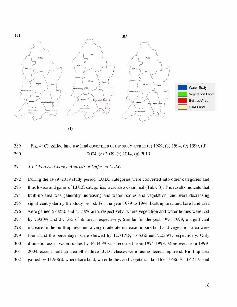
spectral radiance of thermal infrared band to active radiance sensor brightness temperature was 187

calculated by equation 2 (Liu & Zhang, 2011; Maduako et al., 2016; M. Rahman et al., 2017; 188

Sholihah & Shibata, 2019). 189

𝑇𝑖 = 𝐾2ln(𝑘1𝐿𝜆+1) -------------------------------------------- (2) 190

Here, K1 and K2 are the calibration constant; K1 in W/(m2.sr. 𝜇m) and K2 in kelvin respectively. 191

The value of K1 and K2 for Landsat 4-5 and Landsat 8 are given as following Table 2 (Liu & 192

Zhang, 2011). 193

Table 2: Landsat Thermal Bands Calibration Constants 194

Constant Unit K1: W/(m2.sr. μm) Unit K2: Kelvin

Landsat 4-5 TM 607.76 1260.56

Landsat8 TIRS (band 10) 774.8853 1321.0789

Landsat8 TIRS (band 11) 480.8883 1201.1442

c. Retrieving LST: Thermal infrared wavelengths are used to determine Top of Atmosphere 195

(TOA) brightness. Meanwhile, to get an accurate land surface brightness temperature, atmospheric 196

influences such as upward emission and downward irradiance reflected from the surface should be 197

adjusted. Calculating the land surface spectral emissivity (Ɛ) enables the aforementioned 198

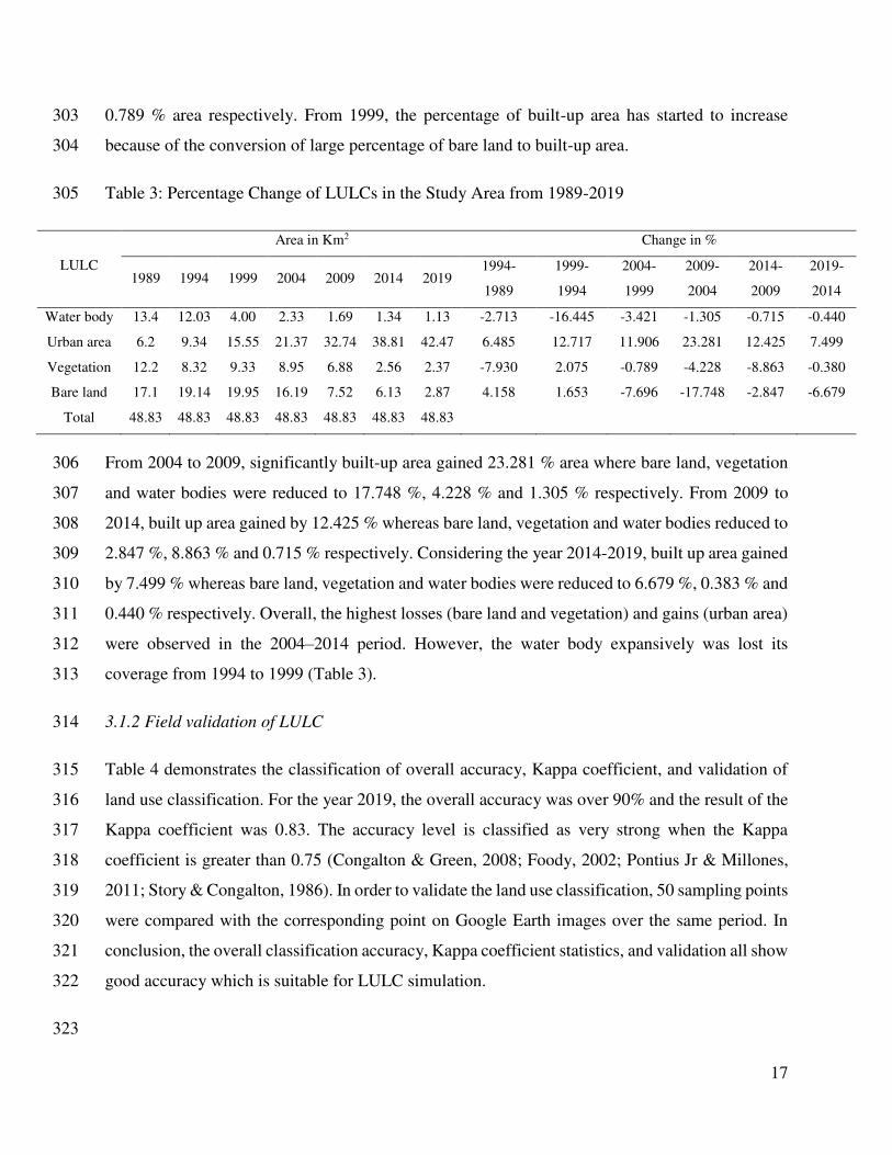
adjustment to be made. Meanwhile, some elements such as water content, chemical composition, 199

structure, and roughness all affect the emissivity of the surface (Zine El Abidine et al., 2014). 200

Numerous scholars have demonstrated that the surface emissivity is highly correlated with the 201

NDVI, and so the emissivity can be calculated using the NDVI (Ahmed et al., 2013). 202

NDVI can be calculated using the following equation 3 using the reflectance values of the Visible 203

and Near Infrared bands (Ahmed et al., 2013). 204

12

NDVI = BNIR−BREDBNIR+BRED ------------------------------------------ (3) 205

Where, BNIR, BRED were the pixel values of near-infrared and red bands. Using the NDVI value 206

the Proportion of Vegetation (Pv) can be calculated to measure land surface emissivity (Ɛ) by using 207

equation 4 (Liu & Zhang, 2011). 208

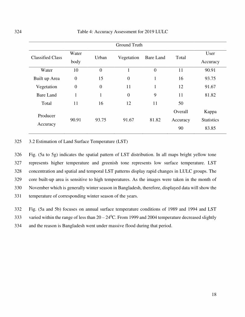
𝑃𝑣 = ( 𝑁𝐷𝑉𝐼−𝑁𝐷𝑉𝐼𝑚𝑖𝑛𝑁𝐷𝑉𝐼− 𝑁𝐷𝑉𝐼𝑚𝑎𝑥)2 -------------------------------------- (4) 209

Using Pv, land surface emissivity (Ɛ) can be measured by following equation 5 (d'Entremont & 210

Thomason, 1987; Good & Giordano, 2019). 211 𝜀 = 0.004 × 𝑃𝑣 + 0.986 ------------------------------------- (5) 212

The land surface temperatures corrected for spectral emissivity (Ɛ) was computed by the following 213

equation 6 (Avdan & Jovanovska, 2016; Chaudhuri & Mishra, 2016; Ullah et al., 2019; Xiong et 214

al., 2012). 215

𝐿𝑆𝑇 = 𝑇𝑖1+(𝜆×𝑇𝑖𝜌 )×ln(𝜀) ---------------------------------------- (6) 216

Here, LST represents land surface temperature; 𝑇𝑖 was the sensors brightness temperature. The 217

emitted radiance’s wavelength was indicated as 𝜆 and Ɛ indicates the land surface spectral 218

emissivity. 219

In addition, 220

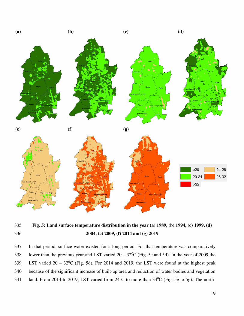
𝜌 = ℎ 𝑐𝜎 ------------------------------------------------ (7) 221

Here, the value of 𝜌 is 1.438×10-2 mk (equation 7). Where h indicates Plank’s constant which is 222

equal to 6.626×10-34 Js, c indicates the velocity of light, which is equal to 2.998×108 ms-2 and 𝜎 is 223

the Boltzmann constant (5.67×10-8 Wm2k-4 = 1.38 ×10-23 JK-1) (Zine El Abidine et al., 2014). 224

Daily temperature data collected from the Bangladesh Meteorological Department (BMD) located 225

at Agargaon, Dhaka was used for validation of estimated LST. 226

13

2.2.3 Simulation of Landcover and LST 227

The CA-ANN model is designed to simulate land-use changes through a multiple output neuron. 228

The network output layer decides the possibilities of multiple land-uses with multiple output 229

neurons. The appropriate parameters for the simulation are calculated automatically by the neural 230

network training process. The CA-ANN model does not include specific transfer rules. The only 231

function is to train the neural network to achieve empirical parameter values. Many factors can be 232

added to the model to improve the precise simulation. A combination of Cellular Automata and 233

ANN Models will produce a better LULC and LST transition spatio-temporal pattern (Mondal, 234

Sharma, Garg, & Kappas, 2016; Parsa, Yavari, & Nejadi, 2016). 235

The LST and LULC for the year 2039 with the help of MOLUSCE plug-in in QGIS 2.18 is 236

typically predicted with an ANN. ANN is an effective method that helps to forecast future LST 237

and LULC using data sets from previous years (Civco, 1993; Z.-L. Li et al., 2013; Maduako et al., 238

2016; Shatnawi & Abu Qdais, 2019). LST simulation was performed in this study using input 239

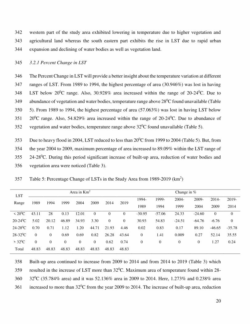
parameters LULC images, NDVI, NDBI, latitude and longitude and as output parameters for LST 240

(Gopal & Woodcock, 1996; Maduako et al., 2016). Besides, the CA-ANN model for the future 241

LULC was used in the prediction of input parameters of road layers, NDBI, NDVI, Latitude and 242

Longitude data. The pixel value data of the images were transformed in ArcGIS software 10.6.1 243

for the better performance of the model. The model was developed using past 20 years data (1999-244

2019) as the input parameters for predicting the future year 2039 data. The LST prediction model 245

architecture is shown in Fig. 3. 246

247

Fig. 3: CA-ANN model architecture 248

14

2.2.4 Field Verification Techniques of LULC 249

The accuracy parameters include the overall accuracy, producer accuracy, user accuracy, and the 250

Kappa coefficients. The overall accuracy is determined by multiplying the error matrix by the total 251

number of corrected samples (equation 8). Historically, the term 'producer accuracy' has been 252

defined as the ratio of the total number of accurate sample units within a category to the total 253

number of sample units within that category (equation 9). This accuracy metric is based on the 254

capability of accurately identifying a reference sample unit and is a real indicator of omission error. 255

When the total number of accurate category sample units is divided by the total number of row 256

sample units on a map (e.g., the total number of row sample units), the result is a commission error 257

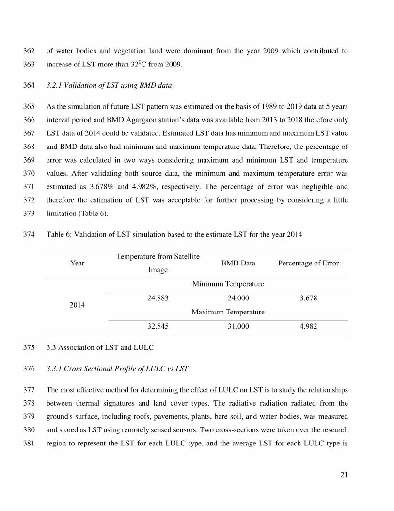
measure. This is referred to as "user accuracy" or "reliability," and it reflects the likelihood that a 258

sample unit specified on the map is actually located on the ground (equation 10). Following the 259

calculation of all accuracy parameters, the Kappa coefficient was determined using equation 11. 260

(Congalton & Green, 2008; Foody, 2002; Pontius Jr & Millones, 2011; Story & Congalton, 1986). 261

𝑂𝑣𝑒𝑟𝑎𝑙 𝐴𝑐𝑐𝑢𝑟𝑎𝑐𝑦 = 𝑇𝑜𝑡𝑎𝑙 𝑛𝑢𝑚𝑏𝑒𝑟 𝑜𝑓 𝑐𝑜𝑟𝑟𝑒𝑐𝑡𝑒𝑑 𝑐𝑙𝑎𝑠𝑠𝑖𝑓𝑖𝑒𝑑 𝑝𝑖𝑥𝑒𝑙𝑥 (𝑑𝑖𝑎𝑔𝑜𝑛𝑎𝑙)𝑡𝑜𝑎𝑙 𝑛𝑢𝑚𝑏𝑒𝑟 𝑜𝑓 𝑟𝑒𝑓𝑒𝑟𝑒𝑛𝑐𝑒 𝑝𝑖𝑥𝑒𝑙𝑠 ∗ 100 --- (8) 262

263

𝑃𝑟𝑜𝑑𝑢𝑐𝑒𝑟 𝐴𝑐𝑐𝑢𝑟𝑎𝑐𝑦 = 𝑛𝑢𝑚𝑏𝑒𝑟 𝑜𝑓 𝑐𝑜𝑟𝑟𝑒𝑐𝑡𝑙𝑦 𝑐𝑙𝑎𝑠𝑠𝑖𝑓𝑖𝑒𝑑 𝑝𝑖𝑥𝑒𝑙𝑥𝑠 𝑖𝑛 𝑒𝑎𝑐ℎ 𝑐𝑎𝑡𝑎𝑔𝑜𝑟𝑦 (𝑑𝑖𝑎𝑔𝑜𝑛𝑎𝑙)𝑡𝑜𝑡𝑎𝑙 𝑛𝑢𝑚𝑏𝑒𝑟 𝑜𝑓 𝑟𝑒𝑓𝑒𝑟𝑒𝑛𝑐𝑒 𝑝𝑖𝑥𝑒𝑙𝑠 𝑖𝑛 𝑒𝑎𝑐ℎ 𝑐𝑎𝑡𝑎𝑔𝑜𝑟𝑦 (𝑐𝑜𝑙𝑢𝑚𝑛 𝑡𝑜𝑡𝑎𝑙) ∗ 100 ---- 264

(9) 265

𝑈𝑠𝑒𝑟 𝐴𝑐𝑐𝑢𝑟𝑎𝑐𝑦 = 𝑛𝑢𝑚𝑏𝑒𝑟 𝑜𝑓 𝑐𝑜𝑟𝑟𝑒𝑐𝑡𝑙𝑦 𝑐𝑙𝑎𝑠𝑠𝑖𝑓𝑖𝑒𝑑 𝑝𝑖𝑥𝑒𝑙𝑥𝑠 𝑖𝑛 𝑒𝑎𝑐ℎ 𝑐𝑎𝑡𝑎𝑔𝑜𝑟𝑦 (𝑑𝑖𝑎𝑔𝑜𝑛𝑎𝑙)𝑡𝑜𝑡𝑎𝑙 𝑛𝑢𝑚𝑏𝑒𝑟 𝑜𝑓 𝑟𝑒𝑓𝑒𝑟𝑒𝑛𝑐𝑒 𝑝𝑖𝑥𝑒𝑙𝑠 𝑖𝑛 𝑒𝑎𝑐ℎ 𝑐𝑎𝑡𝑎𝑔𝑜𝑟𝑦 (𝑟𝑜𝑤 𝑡𝑜𝑡𝑎𝑙) ∗ 100 -- (10) 266

𝐾𝑎𝑝𝑝𝑎 𝐶𝑜𝑒𝑓𝑓𝑖𝑐𝑖𝑒𝑛𝑡 (𝑇) =267 𝑇𝑜𝑡𝑎𝑙 𝑛𝑢𝑚𝑏𝑒𝑟 𝑜𝑓 𝑆𝑎𝑚𝑝𝑙𝑒∗𝑇𝑜𝑡𝑎𝑙 𝑁𝑢𝑚𝑏𝑒𝑟 𝑜𝑓 𝐶𝑜𝑟𝑟𝑒𝑐𝑡𝑒𝑑 𝑆𝑎𝑚𝑝𝑙𝑒− ⅀(𝑐𝑜𝑙.𝑡𝑜𝑡∗𝑟𝑜𝑤 𝑡𝑜𝑡)(𝑇𝑜𝑡𝑎𝑙 𝑛𝑢𝑚𝑏𝑒𝑟 𝑜𝑓 𝑆𝑎𝑚𝑝𝑙𝑒)^2−⅀(𝑐𝑜𝑙.𝑡𝑜𝑡∗𝑟𝑜𝑤 𝑡𝑜𝑡) ∗ 100 ------------ (11) 268

3. Results and Discussions 269

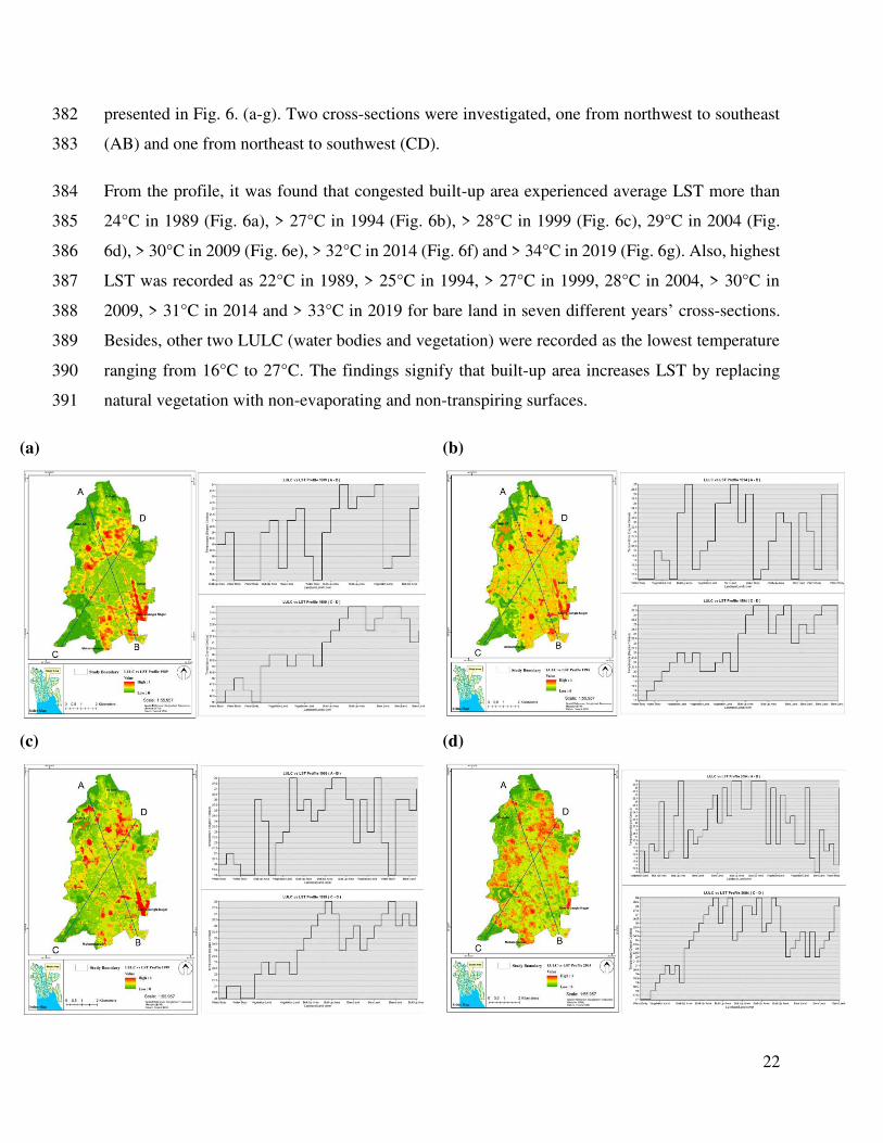
3.1 Land Use Land Cover Classification 270

The LULC map for 1989, 1994, 1999, 2004, 2009, 2014, and 2019 was generated using MLSC 271

(Fig. 4a to 4f). The study's entire area is roughly 48.830 square kilometers. The categorized picture 272

15

from 1989 revealed a larger proportion of area for bare terrain, aquatic bodies, and vegetation, 273

respectively, at 35.04 percent, 27.34 percent, and 24.9 percent. For 1989, the built-up area was just 274

12.56 percent (Fig. 4a). In 1994, bare ground had the most area (39.20 percent), followed by water 275

bodies (24.63 percent) and vegetation (17.04 percent) (Fig. 4b). In 1994, built-up area increased 276

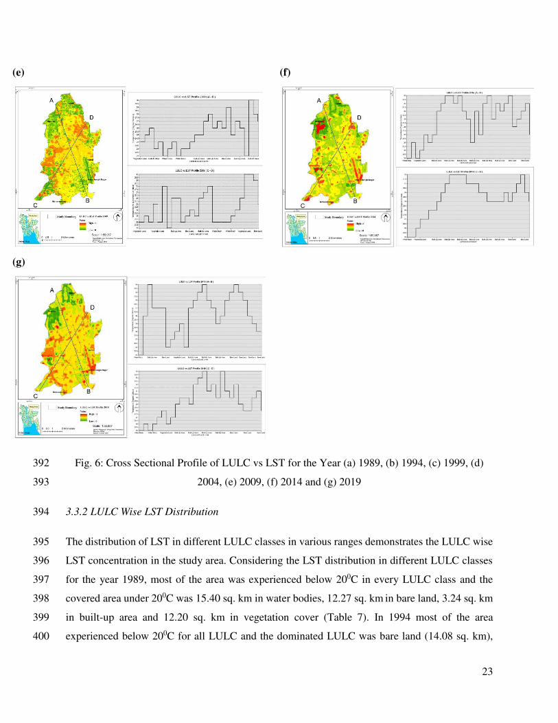
by 7% over 1989 levels. The continuing upward trend in bare land (40.45 percent) and built-up 277

area (31.85 percent) was accelerated in 1999, mostly due to growing urbanization. Water bodies 278

(8.19%) and vegetative land (19.11%) have saw a decline in recent years due to the transfer of 279

natural surfaces to bare ground and later to built-up land (Fig. 4c). In 2004, bare land (33.15 280

percent) continued to decline due to the conversion of bare land to urban built-up areas (43.76 281

percent ). Filling up water bodies (4.77 percent) and vegetative land (18.32 percent) that were 282

initially bare land and were eventually moved to built-up areas began to speed in 2004. (Fig. 4d). 283

The categorized LULC findings for 2009, 2014, and 2019 were compared (Fig. 4e to 4f) by 284

calculating the percentage change in each LULC class over time. Between 2009 and 2019, the 285

quantity of bare and vegetated land decreased considerably (by roughly 10%). During the same 286

time span, the built-up area expanded by a factor of two (21 percent of the study area). Finally, the 287

water body declined by 1% of the studied area between 2009 and 2019. 288

(a)

(b)

(c)

(d)

Pallabi

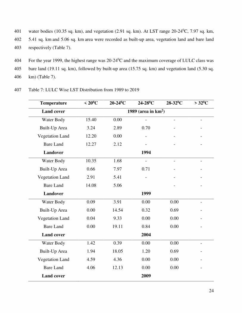
KafrulMirpur

Shah Ali

Mohammadpur

Darus Salam

AdaborSher-e-bangla Nagar

Pallabi

KafrulMirpur

Shah Ali

Mohammadpur

Darus Salam

AdaborSher-e-bangla Nagar

16

(e)

(f)

(g)

Fig. 4: Classified land use land cover map of the study area in (a) 1989, (b) 1994, (c) 1999, (d) 289

2004, (e) 2009, (f) 2014, (g) 2019 290

3.1.1 Percent Change Analysis of Different LULC 291

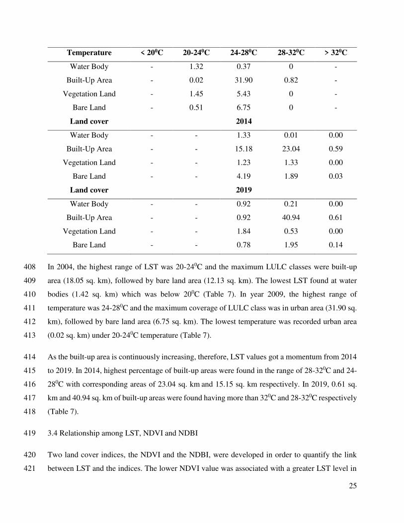
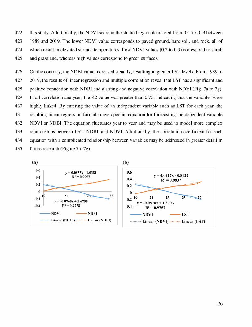
During the 1989–2019 study period, LULC categories were converted into other categories and 292

thus losses and gains of LULC categories, were also examined (Table 3). The results indicate that 293

built-up area was generally increasing and water bodies and vegetation land were decreasing 294

significantly during the study period. For the year 1989 to 1994, built up area and bare land area 295

were gained 6.485% and 4.158% area, respectively, where vegetation and water bodies were lost 296

by 7.930% and 2.713% of its area, respectively. Similar for the year 1994-1999, a significant 297

increase in the built-up area and a very moderate increase in bare land and vegetation area were 298

found and the percentages were showed by 12.717%, 1.653% and 2.056%, respectively. Only 299

dramatic loss in water bodies by 16.445% was recorded from 1994-1999. Moreover, from 1999-300

2004, except built-up area other three LULC classes were facing decreasing trend. Built up area 301

gained by 11.906% where bare land, water bodies and vegetation land lost 7.686 %, 3.421 % and 302

Pallabi

KafrulMirpur

Shah Ali

Mohammadpur

Darus Salam

AdaborSher-e-bangla Nagar

Pallabi

KafrulMirpur

Shah Ali

Mohammadpur

Darus Salam

AdaborSher-e-bangla Nagar

Landcover (2019)

Water Body

Vegetation Land

Built-up Area

Bare Land

Pallabi

KafrulMirpur

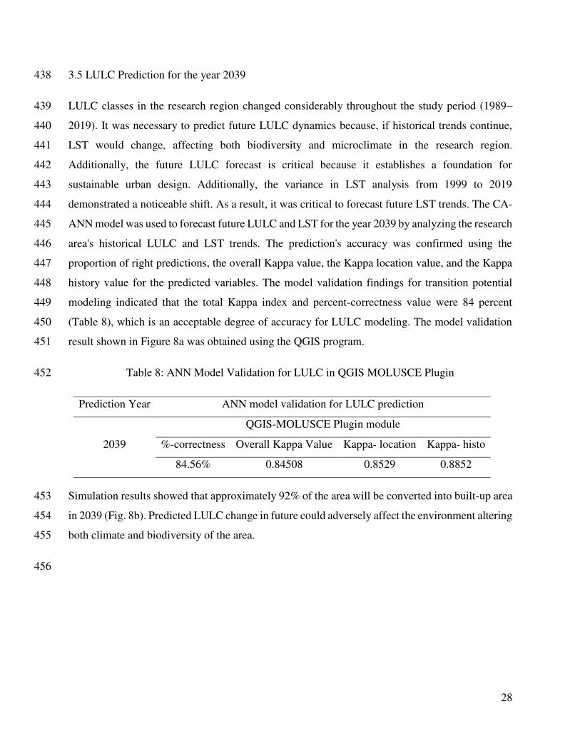
Shah Ali

Mohammadpur

Darus Salam

AdaborSher-e-bangla Nagar

17

0.789 % area respectively. From 1999, the percentage of built-up area has started to increase 303

because of the conversion of large percentage of bare land to built-up area. 304

Table 3: Percentage Change of LULCs in the Study Area from 1989-2019 305

LULC

Area in Km2 Change in %

1989 1994 1999 2004 2009 2014 2019 1994-

1989

1999-

1994

2004-

1999

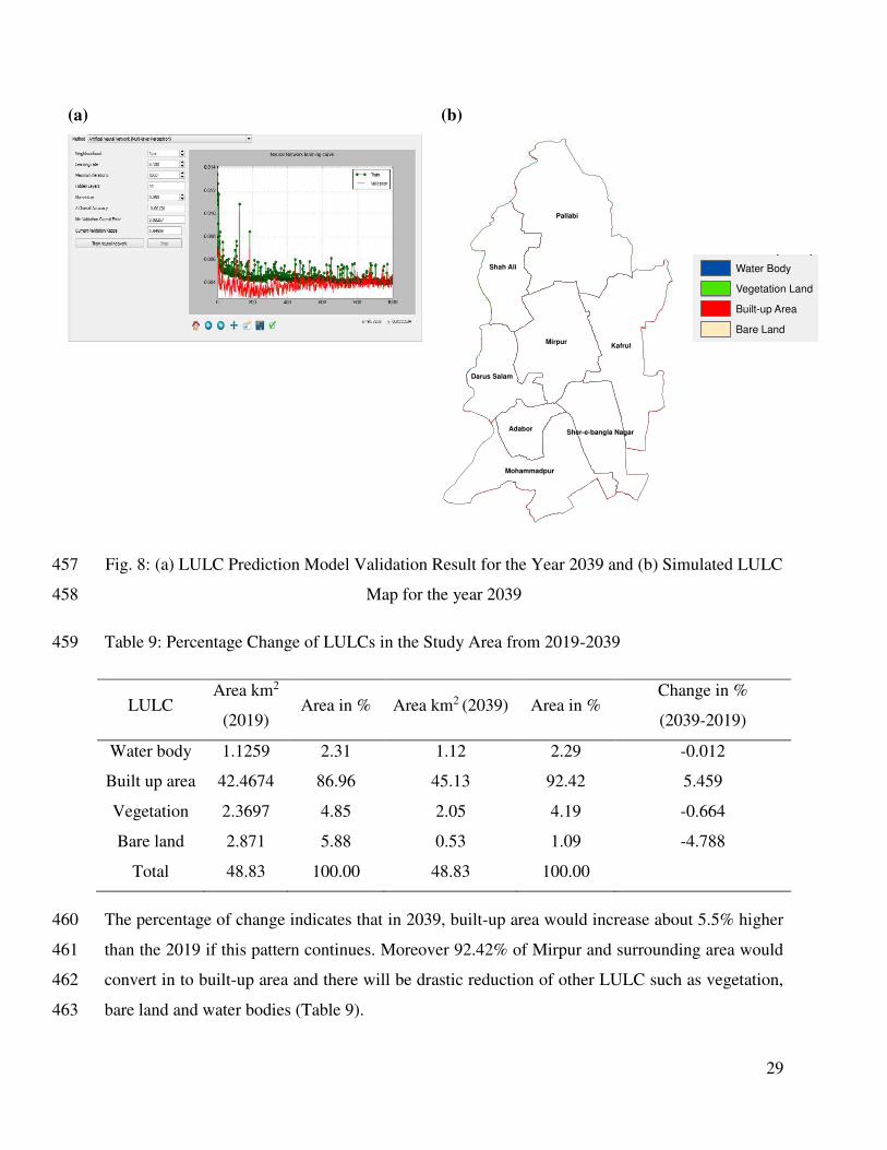
2009-

2004

2014-

2009

2019-

2014

Water body 13.4 12.03 4.00 2.33 1.69 1.34 1.13 -2.713 -16.445 -3.421 -1.305 -0.715 -0.440

Urban area 6.2 9.34 15.55 21.37 32.74 38.81 42.47 6.485 12.717 11.906 23.281 12.425 7.499

Vegetation 12.2 8.32 9.33 8.95 6.88 2.56 2.37 -7.930 2.075 -0.789 -4.228 -8.863 -0.380

Bare land 17.1 19.14 19.95 16.19 7.52 6.13 2.87 4.158 1.653 -7.696 -17.748 -2.847 -6.679

Total 48.83 48.83 48.83 48.83 48.83 48.83 48.83

From 2004 to 2009, significantly built-up area gained 23.281 % area where bare land, vegetation 306

and water bodies were reduced to 17.748 %, 4.228 % and 1.305 % respectively. From 2009 to 307

2014, built up area gained by 12.425 % whereas bare land, vegetation and water bodies reduced to 308

2.847 %, 8.863 % and 0.715 % respectively. Considering the year 2014-2019, built up area gained 309

by 7.499 % whereas bare land, vegetation and water bodies were reduced to 6.679 %, 0.383 % and 310

0.440 % respectively. Overall, the highest losses (bare land and vegetation) and gains (urban area) 311

were observed in the 2004–2014 period. However, the water body expansively was lost its 312

coverage from 1994 to 1999 (Table 3). 313

3.1.2 Field validation of LULC 314

Table 4 demonstrates the classification of overall accuracy, Kappa coefficient, and validation of 315

land use classification. For the year 2019, the overall accuracy was over 90% and the result of the 316

Kappa coefficient was 0.83. The accuracy level is classified as very strong when the Kappa 317

coefficient is greater than 0.75 (Congalton & Green, 2008; Foody, 2002; Pontius Jr & Millones, 318

2011; Story & Congalton, 1986). In order to validate the land use classification, 50 sampling points 319

were compared with the corresponding point on Google Earth images over the same period. In 320

conclusion, the overall classification accuracy, Kappa coefficient statistics, and validation all show 321

good accuracy which is suitable for LULC simulation. 322

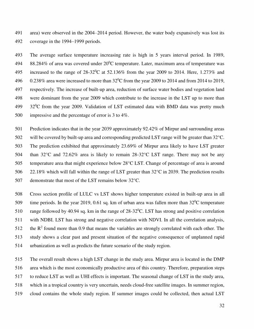
323

18

Table 4: Accuracy Assessment for 2019 LULC 324

Ground Truth

Classified Class Water

body Urban Vegetation Bare Land Total

User

Accuracy

Water 10 0 1 0 11 90.91

Built up Area 0 15 0 1 16 93.75

Vegetation 0 0 11 1 12 91.67

Bare Land 1 1 0 9 11 81.82

Total 11 16 12 11 50

Producer

Accuracy 90.91 93.75 91.67 81.82

Overall

Accuracy

90

Kappa

Statistics

83.85

3.2 Estimation of Land Surface Temperature (LST) 325

Fig. (5a to 5g) indicates the spatial pattern of LST distribution. In all maps bright yellow tone 326

represents higher temperature and greenish tone represents low surface temperature. LST 327

concentration and spatial and temporal LST patterns display rapid changes in LULC groups. The 328

core built-up area is sensitive to high temperatures. As the images were taken in the month of 329

November which is generally winter season in Bangladesh, therefore, displayed data will show the 330

temperature of corresponding winter season of the years. 331

Fig. (5a and 5b) focuses on annual surface temperature conditions of 1989 and 1994 and LST 332

varied within the range of less than 20 – 240C. From 1999 and 2004 temperature decreased slightly 333

and the reason is Bangladesh went under massive flood during that period. 334

19

(a) (b)

(c) (d)

(e)

(f)

(g)

Fig. 5: Land surface temperature distribution in the year (a) 1989, (b) 1994, (c) 1999, (d) 335

2004, (e) 2009, (f) 2014 and (g) 2019 336

In that period, surface water existed for a long period. For that temperature was comparatively 337

lower than the previous year and LST varied 20 – 320C (Fig. 5c and 5d). In the year of 2009 the 338

LST varied 20 – 320C (Fig. 5d). For 2014 and 2019, the LST were found at the highest peak 339

because of the significant increase of built-up area and reduction of water bodies and vegetation 340

land. From 2014 to 2019, LST varied from 240C to more than 340C (Fig. 5e to 5g). The north-341

LST in 2004

<20

20-24

24-28

28-32

>32

20

western part of the study area exhibited lowering in temperature due to higher vegetation and 342

agricultural land whereas the south eastern part exhibits the rise in LST due to rapid urban 343

expansion and declining of water bodies as well as vegetation land. 344

3.2.1 Percent Change in LST 345

The Percent Change in LST will provide a better insight about the temperature variation at different 346

ranges of LST. From 1989 to 1994, the highest percentage of area (30.946%) was lost in having 347

LST below 200C range. Also, 30.928% area increased within the range of 20-240C. Due to 348

abundance of vegetation and water bodies, temperature range above 280C found unavailable (Table 349

5). From 1989 to 1994, the highest percentage of area (57.063%) was lost in having LST below 350

200C range. Also, 54.829% area increased within the range of 20-240C. Due to abundance of 351

vegetation and water bodies, temperature range above 320C found unavailable (Table 5). 352

Due to heavy flood in 2004, LST reduced to less than 200C from 1999 to 2004 (Table 5). But, from 353

the year 2004 to 2009, maximum percentage of area increased to 89.09% within the LST range of 354

24-280C. During this period significant increase of built-up area, reduction of water bodies and 355

vegetation area were noticed (Table 3). 356

Table 5: Percentage Change of LSTs in the Study Area from 1989-2019 (km2) 357

LST

Range

Area in Km2 Change in %

1989 1994 1999 2004 2009 2014 2019 1994-

1989

1999-

1994

2004-

1999

2009-

2004

2014-

2009

2019-

2014

< 200C 43.11 28 0.13 12.01 0 0 0 -30.95 -57.06 24.33 -24.60 0 0

20-240C 5.02 20.12 46.89 34.93 3.30 0 0 30.93 54.83 -24.51 -64.76 -6.76 0

24-280C 0.70 0.71 1.12 1.20 44.71 21.93 4.46 0.02 0.83 0.17 89.10 -46.65 -35.78

28-320C 0 0 0.69 0.69 0.82 26.28 43.64 0 1.41 0.009 0.27 52.14 35.55

> 320C 0 0 0 0 0 0.62 0.74 0 0 0 0 1.27 0.24

Total 48.83 48.83 48.83 48.83 48.83 48.83 48.83

Built-up area continued to increase from 2009 to 2014 and from 2014 to 2019 (Table 3) which 358

resulted in the increase of LST more than 320C. Maximum area of temperature found within 28-359

320C (35.784% area) and it was 52.136% area in 2009 to 2014. Here, 1.273% and 0.238% area 360

increased to more than 320C from the year 2009 to 2014. The increase of built-up area, reduction 361

21

of water bodies and vegetation land were dominant from the year 2009 which contributed to 362

increase of LST more than 320C from 2009. 363

3.2.1 Validation of LST using BMD data 364

As the simulation of future LST pattern was estimated on the basis of 1989 to 2019 data at 5 years 365

interval period and BMD Agargaon station’s data was available from 2013 to 2018 therefore only 366

LST data of 2014 could be validated. Estimated LST data has minimum and maximum LST value 367

and BMD data also had minimum and maximum temperature data. Therefore, the percentage of 368

error was calculated in two ways considering maximum and minimum LST and temperature 369

values. After validating both source data, the minimum and maximum temperature error was 370

estimated as 3.678% and 4.982%, respectively. The percentage of error was negligible and 371

therefore the estimation of LST was acceptable for further processing by considering a little 372

limitation (Table 6). 373

Table 6: Validation of LST simulation based to the estimate LST for the year 2014 374

Year Temperature from Satellite

Image BMD Data Percentage of Error

2014

Minimum Temperature

24.883 24.000 3.678

Maximum Temperature

32.545 31.000 4.982

3.3 Association of LST and LULC 375

3.3.1 Cross Sectional Profile of LULC vs LST 376

The most effective method for determining the effect of LULC on LST is to study the relationships 377

between thermal signatures and land cover types. The radiative radiation radiated from the 378

ground's surface, including roofs, pavements, plants, bare soil, and water bodies, was measured 379

and stored as LST using remotely sensed sensors. Two cross-sections were taken over the research 380

region to represent the LST for each LULC type, and the average LST for each LULC type is 381

22

presented in Fig. 6. (a-g). Two cross-sections were investigated, one from northwest to southeast 382

(AB) and one from northeast to southwest (CD). 383

From the profile, it was found that congested built-up area experienced average LST more than 384

24°C in 1989 (Fig. 6a), > 27°C in 1994 (Fig. 6b), > 28°C in 1999 (Fig. 6c), 29°C in 2004 (Fig. 385

6d), > 30°C in 2009 (Fig. 6e), > 32°C in 2014 (Fig. 6f) and > 34°C in 2019 (Fig. 6g). Also, highest 386

LST was recorded as 22°C in 1989, > 25°C in 1994, > 27°C in 1999, 28°C in 2004, > 30°C in 387

2009, > 31°C in 2014 and > 33°C in 2019 for bare land in seven different years’ cross-sections. 388

Besides, other two LULC (water bodies and vegetation) were recorded as the lowest temperature 389

ranging from 16°C to 27°C. The findings signify that built-up area increases LST by replacing 390

natural vegetation with non-evaporating and non-transpiring surfaces. 391

(a)

(b)

(c)

(d)

23

(e)

(f)

(g)

Fig. 6: Cross Sectional Profile of LULC vs LST for the Year (a) 1989, (b) 1994, (c) 1999, (d) 392

2004, (e) 2009, (f) 2014 and (g) 2019 393

3.3.2 LULC Wise LST Distribution 394

The distribution of LST in different LULC classes in various ranges demonstrates the LULC wise 395

LST concentration in the study area. Considering the LST distribution in different LULC classes 396

for the year 1989, most of the area was experienced below 200C in every LULC class and the 397

covered area under 200C was 15.40 sq. km in water bodies, 12.27 sq. km in bare land, 3.24 sq. km 398

in built-up area and 12.20 sq. km in vegetation cover (Table 7). In 1994 most of the area 399

experienced below 200C for all LULC and the dominated LULC was bare land (14.08 sq. km), 400

24

water bodies (10.35 sq. km), and vegetation (2.91 sq. km). At LST range 20-240C, 7.97 sq. km, 401

5.41 sq. km and 5.06 sq. km area were recorded as built-up area, vegetation land and bare land 402

respectively (Table 7). 403

For the year 1999, the highest range was 20-240C and the maximum coverage of LULC class was 404

bare land (19.11 sq. km), followed by built-up area (15.75 sq. km) and vegetation land (5.30 sq. 405

km) (Table 7). 406

Table 7: LULC Wise LST Distribution from 1989 to 2019 407

Temperature < 200C 20-240C 24-280C 28-320C > 320C

Land cover 1989 (area in km2)

Water Body 15.40 0.00 - - -

Built-Up Area 3.24 2.89 0.70 - -

Vegetation Land 12.20 0.00 - - -

Bare Land 12.27 2.12 - - -

Landover 1994

Water Body 10.35 1.68 - - -

Built-Up Area 0.66 7.97 0.71 - -

Vegetation Land 2.91 5.41 - - -

Bare Land 14.08 5.06 - -

Landover 1999

Water Body 0.09 3.91 0.00 0.00 -

Built-Up Area 0.00 14.54 0.32 0.69 -

Vegetation Land 0.04 9.33 0.00 0.00 -

Bare Land 0.00 19.11 0.84 0.00 -

Land cover 2004

Water Body 1.42 0.39 0.00 0.00 -

Built-Up Area 1.94 18.05 1.20 0.69 -

Vegetation Land 4.59 4.36 0.00 0.00 -

Bare Land 4.06 12.13 0.00 0.00 -

Land cover 2009

25

Temperature < 200C 20-240C 24-280C 28-320C > 320C

Water Body - 1.32 0.37 0 -

Built-Up Area - 0.02 31.90 0.82 -

Vegetation Land - 1.45 5.43 0 -

Bare Land - 0.51 6.75 0 -

Land cover 2014

Water Body - - 1.33 0.01 0.00

Built-Up Area - - 15.18 23.04 0.59

Vegetation Land - - 1.23 1.33 0.00

Bare Land - - 4.19 1.89 0.03

Land cover 2019

Water Body - - 0.92 0.21 0.00

Built-Up Area - - 0.92 40.94 0.61

Vegetation Land - - 1.84 0.53 0.00

Bare Land - - 0.78 1.95 0.14

In 2004, the highest range of LST was 20-240C and the maximum LULC classes were built-up 408

area (18.05 sq. km), followed by bare land area (12.13 sq. km). The lowest LST found at water 409

bodies (1.42 sq. km) which was below 200C (Table 7). In year 2009, the highest range of 410

temperature was 24-280C and the maximum coverage of LULC class was in urban area (31.90 sq. 411

km), followed by bare land area (6.75 sq. km). The lowest temperature was recorded urban area 412

(0.02 sq. km) under 20-240C temperature (Table 7). 413

As the built-up area is continuously increasing, therefore, LST values got a momentum from 2014 414

to 2019. In 2014, highest percentage of built-up areas were found in the range of 28-320C and 24-415

280C with corresponding areas of 23.04 sq. km and 15.15 sq. km respectively. In 2019, 0.61 sq. 416

km and 40.94 sq. km of built-up areas were found having more than 320C and 28-320C respectively 417

(Table 7). 418

3.4 Relationship among LST, NDVI and NDBI 419

Two land cover indices, the NDVI and the NDBI, were developed in order to quantify the link 420

between LST and the indices. The lower NDVI value was associated with a greater LST level in 421

26

this study. Additionally, the NDVI score in the studied region decreased from -0.1 to -0.3 between 422

1989 and 2019. The lower NDVI value corresponds to paved ground, bare soil, and rock, all of 423

which result in elevated surface temperatures. Low NDVI values (0.2 to 0.3) correspond to shrub 424

and grassland, whereas high values correspond to green surfaces. 425

On the contrary, the NDBI value increased steadily, resulting in greater LST levels. From 1989 to 426

2019, the results of linear regression and multiple correlation reveal that LST has a significant and 427

positive connection with NDBI and a strong and negative correlation with NDVI (Fig. 7a to 7g). 428

In all correlation analyses, the R2 value was greater than 0.75, indicating that the variables were 429

highly linked. By entering the value of an independent variable such as LST for each year, the 430

resulting linear regression formula developed an equation for forecasting the dependent variable 431

NDVI or NDBI. The equation fluctuates year to year and may be used to model more complex 432

relationships between LST, NDBI, and NDVI. Additionally, the correlation coefficient for each 433

equation with a complicated relationship between variables may be addressed in greater detail in 434

future research (Figure 7a–7g). 435

(a) (b)

y = -0.0578x + 1.3703

R² = 0.9757

y = 0.0417x - 0.8122

R² = 0.9837

-0.4

-0.2

0

0.2

0.4

0.6

19 21 23 25 27

NDVI LST

Linear (NDVI) Linear (LST)

y = -0.0765x + 1.6755

R² = 0.9778

y = 0.0555x - 1.0381

R² = 0.9957

-0.4

-0.2

0

0.2

0.4

0.6

19 21 23 25

NDVI NDBI

Linear (NDVI) Linear (NDBI)

27

(c)

(d)

(e)

(f)

(g)

Fig. 7: Correlation between LST vs NDVI & NDBI in the year (a) 1989, (b) 1994, (c) 1999, 436

(d) 2004, (e) 2009, (f) 2014 and (g) 2019 437

y = -0.0646x + 1.661

R² = 0.9616

y = 0.047x - 1.0294

R² = 0.9824

-0.4

-0.2

0

0.2

0.4

0.6

19 21 23 25 27 29

NDVI NDBI

Linear (NDVI) Linear (NDBI)

y = -0.0422x + 1.1007

R² = 0.9894

y = 0.034x - 0.6574

R² = 0.9965

-0.2

0

0.2

0.4

0.6

16 21 26

NDVI NDBI

Linear (NDVI) Linear (NDBI)

y = -0.071x + 2.0151

R² = 0.9909

y = 0.0572x - 1.394

R² = 0.9976

-0.2

0

0.2

0.4

0.6

22 24 26 28 30

NDVI NDBI

Linear (NDVI) Linear (NDBI)

y = -0.048x + 1.5603

R² = 0.9738

y = 0.0537x - 1.5944

R² = 0.9292

-0.4

-0.2

0

0.2

0.4

0.6

24 26 28 30 32

NDVI NDBI

Linear (NDVI) Linear (NDBI)

y = -0.0461x + 1.5613

R² = 0.9851

y = 0.0518x - 1.6006

R² = 0.9463

-0.4

-0.2

0

0.2

0.4

0.6

25 27 29 31 33 35

NDVI NDBI

Linear (NDVI) Linear (NDBI)

28

3.5 LULC Prediction for the year 2039 438

LULC classes in the research region changed considerably throughout the study period (1989–439

2019). It was necessary to predict future LULC dynamics because, if historical trends continue, 440

LST would change, affecting both biodiversity and microclimate in the research region. 441

Additionally, the future LULC forecast is critical because it establishes a foundation for 442

sustainable urban design. Additionally, the variance in LST analysis from 1999 to 2019 443

demonstrated a noticeable shift. As a result, it was critical to forecast future LST trends. The CA-444

ANN model was used to forecast future LULC and LST for the year 2039 by analyzing the research 445

area's historical LULC and LST trends. The prediction's accuracy was confirmed using the 446

proportion of right predictions, the overall Kappa value, the Kappa location value, and the Kappa 447

history value for the predicted variables. The model validation findings for transition potential 448

modeling indicated that the total Kappa index and percent-correctness value were 84 percent 449

(Table 8), which is an acceptable degree of accuracy for LULC modeling. The model validation 450

result shown in Figure 8a was obtained using the QGIS program. 451

Table 8: ANN Model Validation for LULC in QGIS MOLUSCE Plugin 452

Prediction Year ANN model validation for LULC prediction

2039

QGIS-MOLUSCE Plugin module

%-correctness Overall Kappa Value Kappa- location Kappa- histo

84.56% 0.84508 0.8529 0.8852

Simulation results showed that approximately 92% of the area will be converted into built-up area 453

in 2039 (Fig. 8b). Predicted LULC change in future could adversely affect the environment altering 454

both climate and biodiversity of the area. 455

456

29

(a)

(b)

Fig. 8: (a) LULC Prediction Model Validation Result for the Year 2039 and (b) Simulated LULC 457

Map for the year 2039 458

Table 9: Percentage Change of LULCs in the Study Area from 2019-2039 459

LULC Area km2

(2019) Area in % Area km2 (2039) Area in %

Change in %

(2039-2019)

Water body 1.1259 2.31 1.12 2.29 -0.012

Built up area 42.4674 86.96 45.13 92.42 5.459

Vegetation 2.3697 4.85 2.05 4.19 -0.664

Bare land 2.871 5.88 0.53 1.09 -4.788

Total 48.83 100.00 48.83 100.00

The percentage of change indicates that in 2039, built-up area would increase about 5.5% higher 460

than the 2019 if this pattern continues. Moreover 92.42% of Mirpur and surrounding area would 461

convert in to built-up area and there will be drastic reduction of other LULC such as vegetation, 462

bare land and water bodies (Table 9). 463

Pallabi

KafrulMirpur

Shah Ali

Mohammadpur

Darus Salam

AdaborSher-e-bangla Nagar

Landcover (2019)

Water Body

Vegetation Land

Built-up Area

Bare Land

30

3.6 LST Prediction for 2039 464

The simulated result showed a strong agreement that confirmed the accuracy of the ANN model’s 465

prediction for 2039 with 91.856% correctness and 0.9362 overall Kappa value (Table 10). Based 466

on the ANN model validation in other researches, the percentage of correctness value over 80% 467

demonstrates strong agreement of accuracy. 468

Table 10: ANN Model Validation for LST in QGIS MOLUSCE Plugin 469

Prediction Year ANN model validation for LST prediction

2039

QGIS-MOLUSCE Plugin module

%-correctness Overall Kappa Value Kappa- location Kappa- histo

91.856 0.9362 0.9037 0.92582

The validation provided an excellent accuracy with more than 90% of correctness for simulated 470

LST map in 2039 (Fig. 9a). Similar to the LULC for the study period from 1989‒2019, LST also 471

shows a substantial amount of change. Accordingly, LST is simulated for 2039. The past trends of 472

estimated LST data are used in the ANN model to predict the future LST trends of the study area. 473

The prediction exhibited that approximately 23.69% of Mirpur area likely to have LST greater 474

than 32°C and 72.62% area is likely to remain 28-32°C LST range. There may not be any 475

temperature area that might experience below 28°C LST. Change of percentage of area is around 476

22.18% which will fall within the range of LST greater than 32°C in 2039 (Table 11). The 477

prediction results demonstrate that most of the LST remains below 32°C. Fig. 9b shows the rising 478

trend of LST in the study area for the year 2039. 479

Table 11: Percentage Change of LSTs in the Study Area from 2019-2039 480

Range Area km2

(2019)

Area in

Percentage

Area km2

(2039)

Area in

Percentage

Change in Percentage

(2039-2019)

< 20°C - - - - -

20-24°C - - - - -

24-28°C 4.46 9.13 1.80 3.69 -5.44

31

28-32°C 43.64 89.36 35.46 72.62 -16.74

> 32°C 0.74 1.51 11.57 23.69 22.18

Total 48.83 100 48.83 100

This effect of high LST is going to be a worrying problem for the study area. The temperature 481

effect depends on the city geometry and Dhaka City's unexpected growth triggers this devastating 482

impact of the increase of LST. 483

(a)

(b)

Fig. 9: (a) LST Prediction Model Validation Result for the Year 2039 and (b) Simulated LST 484

Map for the year 2039 485

4. Conclusions and Recommendations 486

The study area faced tremendous increase of built-up area. Increasing impervious layers trend to 487

reflect and generate higher surface temperature. Considering the year 2014-2019, built-up area 488

gained 7.499 % area where bare land, vegetation and water bodies were lost 6.679%, 0.383% and 489

0.440 % area, respectively. The maximum losses (bare land and vegetation) and gains (built up 490

32

area) were observed in the 2004–2014 period. However, the water body expansively was lost its 491

coverage in the 1994–1999 periods. 492

The average surface temperature increasing rate is high in 5 years interval period. In 1989, 493

88.284% of area was covered under 200C temperature. Later, maximum area of temperature was 494

increased to the range of 28-320C at 52.136% from the year 2009 to 2014. Here, 1.273% and 495

0.238% area were increased to more than 320C from the year 2009 to 2014 and from 2014 to 2019, 496

respectively. The increase of built-up area, reduction of surface water bodies and vegetation land 497

were dominant from the year 2009 which contribute to the increase in the LST up to more than 498

320C from the year 2009. Validation of LST estimated data with BMD data was pretty much 499

impressive and the percentage of error is 3 to 4%. 500

Prediction indicates that in the year 2039 approximately 92.42% of Mirpur and surrounding areas 501

will be covered by built-up area and corresponding predicted LST range will be greater than 32°C. 502

The prediction exhibited that approximately 23.69% of Mirpur area likely to have LST greater 503

than 32°C and 72.62% area is likely to remain 28-32°C LST range. There may not be any 504

temperature area that might experience below 28°C LST. Change of percentage of area is around 505

22.18% which will fall within the range of LST greater than 32°C in 2039. The prediction results 506

demonstrate that most of the LST remains below 32°C. 507

Cross section profile of LULC vs LST shows higher temperature existed in built-up area in all 508

time periods. In the year 2019, 0.61 sq. km of urban area was fallen more than 320C temperature 509

range followed by 40.94 sq. km in the range of 28-320C. LST has strong and positive correlation 510

with NDBI. LST has strong and negative correlation with NDVI. In all the correlation analysis, 511

the R2 found more than 0.9 that means the variables are strongly correlated with each other. The 512

study shows a clear past and present situation of the negative consequence of unplanned rapid 513

urbanization as well as predicts the future scenario of the study region. 514

The overall result shows a high LST change in the study area. Mirpur area is located in the DMP 515

area which is the most economically productive area of this country. Therefore, preparation steps 516

to reduce LST as well as UHI effects is important. The seasonal change of LST in the study area, 517

which in a tropical country is very uncertain, needs cloud-free satellite images. In summer region, 518

cloud contains the whole study region. If summer images could be collected, then actual LST 519

33

effects can easily be realized. In addition, to understand the magnitude, it is necessary to evaluate 520

UHI locally and nationwide. 521

To the Author's knowledge, this is the first research to provide a method for estimating future LST 522

of metropolitan areas from observable connections between land cover and LST changes in the 523

study region. Since a result, future city planning should place a greater emphasis on urban 524

greening, as the research region increasingly shifts towards the highest temperature zone owing to 525

urbanization. If current trends continue, by 2039, nearly the whole study region will be a UHI. A 526

compact-town-style decentralization of metropolitan regions (satellite-towns) is therefore a viable 527

path ahead for preventing the future creation of large-scale UHI effects. The work derived future 528

LST using LULC indices (NDVI and NDBI) and a simple regression equation. It is feasible to 529

combine the various land cover indices as independent variables in a multiple regression equation 530

model in order to calculate the LST in a more robust manner, potentially using factor analysis. 531

Future research should integrate these elements and strive to improve upon the model given here. 532

Acknowledgment 533

All praises to Allah the benevolent, the Almighty, and the kind. We wish to express my profound 534

gratitude and sincere appreciation to Mohammad Shahriyar Parvez, Research Assistant, 535

Department of Civil Engineering, Military Institute of Science and Technology (MIST), for his 536

untiring help in preparing this research work. 537

Contributions 538

A N M Foyezur Rahman: methodology, software, data curation, writing—original draft 539

preparation. 540

M Tauhid Ur Rahman: conceptualization, methodology, writing—review & editing. 541

Ethics approval 542

Not applicable 543

Consent to participate 544

34

Agree to participate 545

Consent for publication 546

Agree to publish 547

Competing interests 548

The author declares that this research work is his original work and has written it in its entirety. 549

He has duly acknowledged all the sources of information that have been used in the paper. 550

Funding 551

This study was not funded. 552

Data Availability 553

The datasets used and analysed during the current study are available from the corresponding 554

author on reasonable request. 555

References 556

Ahmed, B. (2011a). Modelling spatio-temporal urban land cover growth dynamics using remote 557

sensing and GIS techniques: A case study of Khulna City. Journal of Bangladesh institute 558

of Planners, 4, 15-32. 559

Ahmed, B. (2011b). Urban land cover change detection analysis and modeling spatio-temporal 560

Growth dynamics using Remote Sensing and GIS Techniques: A case study of Dhaka, 561

Bangladesh. 562

Ahmed, B., Kamruzzaman, M., Zhu, X., Rahman, M. S., & Choi, K. (2013). Simulating land cover 563

changes and their impacts on land surface temperature in Dhaka, Bangladesh. Remote 564

Sensing, 5(11), 5969-5998. 565

Al-sharif, A. A. A., & Pradhan, B. (2014). Monitoring and predicting land use change in Tripoli 566

Metropolitan City using an integrated Markov chain and cellular automata models in GIS. 567

Arabian journal of geosciences, 7(10), 4291-4301. 568

35

Amiri, R., Weng, Q., Alimohammadi, A., & Alavipanah, S. K. (2009). Spatial–temporal dynamics 569

of land surface temperature in relation to fractional vegetation cover and land use/cover in 570

the Tabriz urban area, Iran. Remote sensing of environment, 113(12), 2606-2617. 571

Arsanjani, J. J., Helbich, M., Kainz, W., & Boloorani, A. D. (2013). Integration of logistic 572

regression, Markov chain and cellular automata models to simulate urban expansion. 573

International Journal of Applied Earth Observation and Geoinformation, 21, 265-275. 574

Avdan, U., & Jovanovska, G. (2016). Algorithm for automated mapping of land surface 575

temperature using LANDSAT 8 satellite data. Journal of Sensors, 2016. 576

Bahi, H., Rhinane, H., Bensalmia, A., Fehrenbach, U., & Scherer, D. (2016). Effects of 577

urbanization and seasonal cycle on the surface urban heat island patterns in the coastal 578

growing cities: A case study of Casablanca, Morocco. Remote Sensing, 8(10), 829. 579

Balogun, I., & Ishola, K. (2017). Projection of future changes in landuse/landcover using cellular 580

automata/markov model over Akure city, Nigeria. Journal of Remote Sensing Technology, 581

5(1), 22-31. 582

Celik, B., Kaya, S., Alganci, U., & Seker, D. Z. (2019). Assessment of the Relationship Between 583

Land Use/Cover Changes and Land Surface Temperatures: A case study of Thermal 584

Remote Sensing. FEB-FRESENIUS ENVIRONMENTAL BULLETIN, 3, 541. 585

Chander, G., Markham, B. L., & Helder, D. L. (2009). Summary of current radiometric calibration 586

coefficients for Landsat MSS, TM, ETM+, and EO-1 ALI sensors. Remote sensing of 587

environment, 113(5), 893-903. 588

Chaudhuri, G., & Mishra, N. B. (2016). Spatio-temporal dynamics of land cover and land surface 589

temperature in Ganges-Brahmaputra delta: A comparative analysis between India and 590

Bangladesh. Applied geography, 68, 68-83. 591

Chen, X.-L., Zhao, H.-M., Li, P.-X., & Yin, Z.-Y. (2006). Remote sensing image-based analysis 592

of the relationship between urban heat island and land use/cover changes. Remote sensing 593

of environment, 104(2), 133-146. 594

Civco, D. L. (1993). Artificial neural networks for land-cover classification and mapping. 595

International journal of geographical information science, 7(2), 173-186. 596

Congalton, R. G., & Green, K. (2008). Assessing the accuracy of remotely sensed data: principles 597

and practices: CRC press. 598

36

Corner, R. J., Dewan, A. M., & Chakma, S. (2014). Monitoring and prediction of land-use and 599

land-cover (LULC) change. In Dhaka megacity (pp. 75-97): Springer. 600

d'Entremont, R. P., & Thomason, L. W. (1987). Interpreting meteorological satellite images using 601

a color-composite technique. Bulletin of the American Meteorological Society, 68(7), 762-602

768. 603

Dewan, A. M., Kabir, M. H., Nahar, K., & Rahman, M. Z. (2012). Urbanisation and environmental 604

degradation in Dhaka Metropolitan Area of Bangladesh. International Journal of 605

Environment and Sustainable Development, 11(2), 118-147. 606

Dewan, A. M., & Yamaguchi, Y. (2009). Land use and land cover change in Greater Dhaka, 607

Bangladesh: Using remote sensing to promote sustainable urbanization. Applied 608

geography, 29(3), 390-401. 609

Foody, G. M. (2002). Status of land cover classification accuracy assessment. Remote sensing of 610

environment, 80(1), 185-201. 611

Fu, P., & Weng, Q. (2018). Responses of urban heat island in Atlanta to different land-use 612

scenarios. Theoretical and applied climatology, 133(1-2), 123-135. 613

Good, T., & Giordano, P. A. (2019). Methods for constructing a color composite image. In: Google 614

Patents. 615

Gopal, S., & Woodcock, C. (1996). Remote sensing of forest change using artificial neural 616

networks. IEEE Transactions on Geoscience and Remote Sensing, 34(2), 398-404. 617

Grimmond, S. U. E. (2007). Urbanization and global environmental change: local effects of urban 618

warming. Geographical Journal, 173(1), 83-88. 619

Gutman, G., Huang, C., Chander, G., Noojipady, P., & Masek, J. G. (2013). Assessment of the 620

NASA–USGS global land survey (GLS) datasets. Remote sensing of environment, 134, 621

249-265. 622

Handayanto, R. T., Kim, S. M., & Tripathi, N. K. (2017, 2017). Land use growth simulation and 623

optimization in the urban area. 624

Hart, M. A., & Sailor, D. J. (2009). Quantifying the influence of land-use and surface 625

characteristics on spatial variability in the urban heat island. Theoretical and applied 626

climatology, 95(3-4), 397-406. 627

IPCC. (2014). Mitigation of climate change. Contribution of Working Group III to the Fifth 628

Assessment Report of the Intergovernmental Panel on Climate Change, 1454. 629

37

Islam, M. S., & Ahmed, R. (2011). Land use change prediction in Dhaka city using GIS aided 630

Markov chain modeling. Journal of Life and Earth Science, 6, 81-89. 631

Kafy, A., Islam, M., Ferdous, L., Khan, A. R., & Hossain, M. M. (2019). Identifying Most 632

Influential Land Use Parameters Contributing Reduction of Surface Water Bodies in 633

Rajshahi City, Bangladesh: A Remote Sensing Approach. Remote Sensing of Land, 2(2), 634

87-95. doi:http://dx.doi.org/10.21523/gcj1.18020202 635

Lambin, E. F. (1999). Land-use and land-cover Change (LUCC)-implementation strategy. A core 636

project of the International Geosphere-Biosphere Programme and the International 637

Human Dimensions Programme on Global Environmental Change. 638

Li, J., & Zhao, H. (2003). Detecting urban land-use and land-cover changes in Mississauga using 639

Landsat TM images. Journal of Environmental Informatics, 2(1), 38-47. 640

Li, Z.-L., Tang, B.-H., Wu, H., Ren, H., Yan, G., Wan, Z., . . . Sobrino, J. A. (2013). Satellite-641

derived land surface temperature: Current status and perspectives. Remote sensing of 642

environment, 131, 14-37. 643

Lilly Rose, A., Devadas, M.D., . , . (2009). Analysis of Land Surface Temperature and Land 644

Use/Land Cover Types Using Remote Sensing Imagery - A Case In Chennai City, 645

India. Paper presented at the The seventh International Conference on Urban Climate., held on 29 646

June – 3 July 2009, Yokohama, Japan. 647

Liu, L., & Zhang, Y. (2011). Urban heat island analysis using the Landsat TM data and ASTER 648

data: A case study in Hong Kong. Remote Sensing, 3(7), 1535-1552. 649

Maduako, I. D., Yun, Z., & Patrick, B. (2016). Simulation and prediction of land surface 650

temperature (LST) dynamics within Ikom City in Nigeria using artificial neural network 651

(ANN). Journal of Remote Sensing & GIS, 5(1), 1-7. 652

Maimaitiyiming, M., Ghulam, A., Tiyip, T., Pla, F., Latorre-Carmona, P., Halik, Ü., . . . Caetano, 653

M. (2014). Effects of green space spatial pattern on land surface temperature: Implications 654

for sustainable urban planning and climate change adaptation. ISPRS journal of 655

photogrammetry and remote sensing, 89, 59-66. 656

McKinney, M. L. (2002). Urbanization, biodiversity, and conservation. Bioscience 52: 657

883890McKinney ML (2006) Urbanization as a major cause of biotic homogenization. 658

Biol Conserv, 127, 247260. 659

38

Meyer, W. B., & Turner, B. L. (1992). Human population growth and global land-use/cover 660

change. Annual review of ecology and systematics, 23(1), 39-61. 661

Mishra, V. N., & Rai, P. K. (2016). A remote sensing aided multi-layer perceptron-Markov chain 662

analysis for land use and land cover change prediction in Patna district (Bihar), India. 663

Arabian journal of geosciences, 9(4), 249. 664

Mondal, M. S., Sharma, N., Garg, P., & Kappas, M. (2016). Statistical independence test and 665

validation of CA Markov land use land cover (LULC) prediction results. The Egyptian 666

Journal of Remote Sensing and Space Science, 19(2), 259-272. 667

Mozumder, C., & Tripathi, N. K. (2014). Geospatial scenario based modelling of urban and 668

agricultural intrusions in Ramsar wetland Deepor Beel in Northeast India using a multi-669

layer perceptron neural network. International Journal of Applied Earth Observation and 670

Geoinformation, 32, 92-104. 671

Parsa, V. A., Yavari, A., & Nejadi, A. (2016). Spatio-temporal analysis of land use/land cover 672

pattern changes in Arasbaran Biosphere Reserve: Iran. Modeling Earth Systems and 673

Environment, 2(4), 1-13. 674

Pontius Jr, R. G., & Millones, M. (2011). Death to Kappa: birth of quantity disagreement and 675

allocation disagreement for accuracy assessment. International Journal of Remote Sensing, 676

32(15), 4407-4429. 677

Rahman, M. (2016). Detection of land use/land cover changes and urban sprawl in Al-Khobar, 678

Saudi Arabia: An analysis of multi-temporal remote sensing data. ISPRS International 679

Journal of Geo-Information, 5(2), 15. 680

Rahman, M., Aldosary, A. S., & Mortoja, M. (2017). Modeling future land cover changes and their 681

effects on the land surface temperatures in the Saudi Arabian eastern coastal city of 682

Dammam. Land, 6(2), 36. 683

Rahman, M. S., Mohiuddin, H., Kafy, A.-A., Sheel, P. K., & Di, L. (2018). Classification of cities 684

in Bangladesh based on remote sensing derived spatial characteristics. Journal of Urban 685

Management. 686

Rahman, M. T., Aldosary, A. S., & Mortoja, M. (2017). Modeling future land cover changes and 687

their effects on the land surface temperatures in the Saudi Arabian eastern coastal city of 688

Dammam. Land, 6(2), 36. 689

39

Rahman, M. T., & Rashed, T. (2015). Urban tree damage estimation using airborne laser scanner 690

data and geographic information systems: An example from 2007 Oklahoma ice storm. 691

Urban Forestry & Urban Greening, 14(3), 562-572. 692

Santé, I., García, A. M., Miranda, D., & Crecente, R. (2010). Cellular automata models for the 693

simulation of real-world urban processes: A review and analysis. Landscape and urban 694

planning, 96(2), 108-122. 695

Scarano, M., & Sobrino, J. A. (2015). On the relationship between the sky view factor and the land 696

surface temperature derived by Landsat-8 images in Bari, Italy. International Journal of 697

Remote Sensing, 36(19-20), 4820-4835. 698

Shatnawi, N., & Abu Qdais, H. (2019). Mapping urban land surface temperature using remote 699

sensing techniques and artificial neural network modelling. International Journal of 700

Remote Sensing, 1-16. 701

Sholihah, R. I., & Shibata, S. (2019). Retrieving Spatial Variation of Land Surface Temperature 702

Based on Landsat OLI/TIRS: A Case of Southern part of Jember, Java, Indonesia. Paper 703

presented at the IOP Conference Series: Earth and Environmental Science. 704

Story, M., & Congalton, R. G. (1986). Accuracy assessment: a user’s perspective. 705

Photogrammetric Engineering and remote sensing, 52(3), 397-399. 706

Streutker, D. R. (2003). Satellite-measured growth of the urban heat island of Houston, Texas. 707

Remote sensing of environment, 85(3), 282-289. 708

Thapa, R., & Murayama, Y. (2009). Examining spatiotemporal urbanization patterns in 709

Kathmandu Valley, Nepal: Remote sensing and spatial metrics approaches. Remote 710

Sensing, 1(3), 534-556. 711

Tran, D. X., Pla, F., Latorre-Carmona, P., Myint, S. W., Caetano, M., & Kieu, H. V. (2017). 712

Characterizing the relationship between land use land cover change and land surface 713

temperature. ISPRS journal of photogrammetry and remote sensing, 124, 119-132. 714

Ullah, S., Tahir, A. A., Akbar, T. A., Hassan, Q. K., Dewan, A., Khan, A. J., & Khan, M. (2019). 715

Remote sensing-based quantification of the relationships between land use land cover 716

changes and surface temperature over the lower Himalayan region. Sustainability, 11(19), 717

5492. 718

van Scheltinga, C. T., Quadir, D. A., & Ludwig, F. (2015). Baseline Study Climate Change–719

Bangladesh Delta Plan. Retrieved from 720

40

Weng, Q., Lu, D., & Schubring, J. (2004). Estimation of land surface temperature–vegetation 721

abundance relationship for urban heat island studies. Remote sensing of environment, 722

89(4), 467-483. 723

Xiong, Y., Huang, S., Chen, F., Ye, H., Wang, C., & Zhu, C. (2012). The impacts of rapid 724

urbanization on the thermal environment: A remote sensing study of Guangzhou, South 725

China. Remote Sensing, 4(7), 2033-2056. 726

Yu, X., Guo, X., & Wu, Z. (2014). Land surface temperature retrieval from Landsat 8 TIRS—727

Comparison between radiative transfer equation-based method, split window algorithm 728

and single channel method. Remote Sensing, 6(10), 9829-9852. 729

Zheng, H. W., Shen, G. Q., Wang, H., & Hong, J. (2015). Simulating land use change in urban 730

renewal areas: A case study in Hong Kong. Habitat International, 46, 23-34. 731

Zhi-hao, Q., Wen-juan, L., Ming-hua, Z., Karnieli, A., & Berliner, P. (2011). Estimating of the 732

essential atmospheric parameters of mono-window algorithm for land surface temperature 733

retrieval from Landsat TM 6. Remote Sensing for Land & Resources, 15(2), 37-43. 734

Zhou, W., Huang, G., & Cadenasso, M. L. (2011). Does spatial configuration matter? 735

Understanding the effects of land cover pattern on land surface temperature in urban 736

landscapes. Landscape and urban planning, 102(1), 54-63. 737

Zine El Abidine, E. M., Mohieldeen, Y. E., Mohamed, A. A., Modawi, O., & Al-Sulaiti, M. H. 738

(2014). Heat wave hazard modelling: Qatar case study. QScience connect, 9. 739