Use of Energy-storage Equipped Shunt Compensator for Frequency Control

Master of Science Thesis in the Master Degree Programme, Electric Power

Engineering

MATHIAS H. NORDLUND Department of Energy and Environment Division of Electric Power Engineering

CHALMERS UNIVERSITY OF TECHNOLOGY Göteborg, Sweden, 2010

Use of Energy-storage Equipped Shunt Compensator for Frequency Control MATHIAS H. NORDLUND Department of Energy and Environment CHALMERS UNIVERSITY OF TECHNOLOGY Göteborg, Sweden 2010

Use of Energy-storage Equipped Shunt Compensator for Frequency Control © MATHIAS H. NORDLUND, 2010 Department of Energy and Environment Chalmers University of Technology SE-412 96 Göteborg Sweden Telephone + 46 (0)31-772 1000

Mater thesis conducted at Chalmers University of technology in cooperation with Falbygdens Energi AB (FEAB) and ABB

Chalmers Bibliotek, Reproservice Göteborg, Sweden 2010

Acknowledgment

I owe my deepest gratitude to all those that have helped me conduct this thesis and I am honored that I had the opportunity to work with all these people.

Lars Ohlsson from Falbygdens Energi AB – For providing the project to be conducted and for support during the project.

Per Halvarsson & Lars Apell from ABB – For providing information and ideas about the project, also for support throughout the project.

Massimo Bongiorno from Chalmers University of Technology – For putting his trust in me and giving me the opportunity to conduct this master thesis. Also for all the support, both concerning the project and for personal issues.

Francisco Montes Venero – For providing the PSCAD model of the FEAB grid and for support during the project.

I thank all of you for this time and I hope that this was not the last time that we worked together.

Mathias Nordlund

Gothenburg, Sweden

June, 2010

Abstract

The continuous growth of the electrical system, resulting in growing electric power demand, is putting great emphasis on system operation and control. These topics, together with system reliability and security, are becoming more and more of interest for the research community, in particular due to the recent trend towards restructuring and deregulation of the power supplies. It is under this scenario that Flexible AC Transmission Systems (FACTS) Controllers at transmission level and Custom Power Devices at distribution level represent both opportunities and challenges for an optimal use of the power systems. In particular, the Static Synchronous Compensator (STATCOM) is a key device for reinforcement of the stability in an AC power system and for mitigation of power quality phenomena. Although typically used for reactive power injection only, an upcoming idea today is to equip the STATCOM with an energy storage connected on the dc-link of the converter, thus also allowing short-term active power support to the power systems. This report focuses on the use of energy storage equipped STATCOM (also known under the name of E-STATCOM). As first, the current controller used in the compensator, which represents the heart of the control system, will be derived. Then, two additional control systems, in order to allow frequency control and power oscillation damping, will be derived and analyzed. To verify these control systems, a simple network will be used as a benchmark model in PSCAD/EMTDC and the results from the simulations will be analyzed. The obtained results on the stability improvement by aims of the E-STATCOM will be supported by analytical investigation. Furthermore, the need for active power support in the actual grid of Falbygdens Energi AB (FEAB) will be investigated. Finally, the impact of a controllable load, or “smart load”, on the dynamic performance of the investigated FEAB’s grid will be shown. In the investigated cases, the smart load will be controlled in order to meet the power balance between load and local production in case of islanding conditions. The obtained results show good dynamical performance of the system. By analyzing the results from the simulations it can be concluded that it is possible to temporary control the system frequency, given an adequate size of the energy storage. The size of the storage is of high importance, in particular in case of islanding operation. It will be shown that another important factor for a successful operation of the E-STATCOM is its location into the power system. The location of the compensator will impact the dynamic performance of the overall system as well as the energy storage ratings, in particular when used for power oscillation damping.

Table of content

Chapter 1. Introduction ........................................................................................... 1

1.1 Background and motivations ......................................................................... 1

1.2 Previous research ........................................................................................... 2

1.3 Problem setup ................................................................................................ 2

Chapter 2. Static synchronous compensator - E-STATCOM ................................ 3

2.1 Voltage source converter – VSC .................................................................... 3

2.2 Application for E-STATCOM ....................................................................... 5

2.3 Representation in PSCAD ............................................................................. 6

2.4 Control systems ............................................................................................. 8

2.5 Current controller .......................................................................................... 9

2.6 Voltage controller ........................................................................................ 12

2.7 Frequency controller .................................................................................... 13

2.7.1 Droop ......................................................................................................... 15

2.8 Power oscillation damping controller ........................................................... 16

2.9 Modeling of Energy Storage ........................................................................ 18

2.10 Synchronization system ............................................................................... 19

2.10.1 Traditional Phase-Locked Loop (PLL) ...................................................... 19

2.10.2 Auto-Normalizing Phase-Locked Loop (AN-PLL).................................... 20

Chapter 3. Power oscillation damping................................................................... 23

3.1 Analytical investigation ............................................................................... 23

3.1.1 Small signal stability without E-STATCOM ............................................... 24

3.1.2 Small signal stability with E-STATCOM .................................................... 26

3.1.3 Comparison with and without E-STATCOM .............................................. 27

3.2 Simulations on power oscillation damping ................................................... 28

3.3 Impact on PCC for power oscillation damping ............................................. 29

Chapter 4. Simulation results ................................................................................ 31

4.1 Frequency control ........................................................................................ 31

4.2 Power oscillation damping ........................................................................... 35

Chapter 5. Falbygdens Energi AB ......................................................................... 37

5.1 Grid setup .................................................................................................... 37

5.2 Simulation results ........................................................................................ 38

5.2.1 Three phase to ground fault & voltage dip .................................................. 38

5.2.2 Fluctuating power from wind farms ............................................................ 41

5.2.3 System islanding......................................................................................... 43

5.2.4 Islanding mode without “smart load” .......................................................... 43

5.2.5 Islanding mode with “smart load” ............................................................... 47

Chapter 6. Conclusions and Future work ............................................................. 51

6.1 Falbygdens Energi AB ................................................................................. 52

6.2 Future work ................................................................................................. 53

APPENDIX ............................................................................................................... 55

Reference list ............................................................................................................. 57

1

Chapter 1. Introduction

1.1 Background and motivations

The traditional way of producing power is to have a small number of large power plants, which in Sweden are often located far away from where the power is needed. The trend of today is to increase the renewable energy sources and have more small scale production distributed in the grid. This together with new applications as large power storage devices and “smart loads” among other things will create a reliable and sustainable production of electricity. It will also increase the efficiency of the already existing grid so that it will be easier to meet the increase in demand of power. This is an important part of the “smart grid” concept. The small scale production consists of different types of renewable energy sources such as solar power, wave power and wind power. All of these are dependent on the type of weather and can therefore vary a lot during the day. The production planning is based on weather forecast and is consequently not completely reliable. Due to this there has to be some options so that power can be delivered at all times without any interruptions. Wind power is one renewable energy source that is based on forecast and it is also the fastest increasing renewable energy source today. The reason for the increase of wind power is due to the fact that the green house effect has to be prevented at the same time as the power usage in the world is increasing. Today 2.5 TWh is produced from wind power in Sweden every year and the goal is to have 30TWh year 2020 [13]. According to these numbers, the growth of wind power will continue. One important thing to remember is that when a large amount of wind power is installed into the grid, some part of it could be weakened. To cope with this, new technologies has to be used to provide a safe and sustainable electricity production. Also due to the uncertainties in the production from wind power, there has to be some back up. Energy storage is one option to the above stated problem. It is also an interesting area since it can provide additional features which can be related to the “smart grid”. The main use of energy storage is to store energy when the produced power exceeds the used. This power can then be sold when the demand instead is high, which often is during the days. In addition to this it can help to increase the stability of the system, especially if the grid is weak. As mentioned this is the case especially when a large amount of wind power is used. This technology is therefore very useful for applications when large amount of wind power, or some other type of renewable, is present in the grid. This report will focus on the impact of using energy storage devices together with a static synchronous compensator (STATCOM) to have a reliable operation of the grid. Further down in this report the acronym for this device will be E-STATCOM (Energy storage equipped static synchronous compensator). The energy storage device in the grid is one new application that will be used in the future grid to increase the reliability.

2

1.2 Previous research

There has been some research ongoing of using an E-STATCOM for different applications in the grid, especially together with wind farms. In [8] the use of E-STATCOM for smoothing out intermittent wind farm power is discussed. This is interesting particularly in the case of weak grids since it in this case could cause power quality issues, such as fluctuating voltage or frequency variations. How to control the E-STATCOM is also treated in this paper. The latest is also done in article [9] where the main focus is on how to control the E-STATCOM. The result given in both articles shows that a STATCOM attached with a proper energy storage device will be able to smooth out the power to avoid power quality issues and to store spare power. Research has also been done in the area of increasing the stability in the grid. In [10] the dynamic performance of the E-STATCOM is instead investigated to see the impact when participating in the primary reserve for frequency control. The idea is to aid the primary frequency control during a short period of time when for example the blades of a turbine are pitched to adjust the mechanical torque. The capability of aiding the primary reserve is though dependent on the size of the energy storage. Another issue that can occur in the grid and cause severe problems is phase angle jumps which are often associated with voltage dips. This can cause problems for AC motors and their drives since a phase angle jump can cause it to trip. It is shown in [1] that this problem can be reduced significantly by using a STATCOM together with energy storage, in this case capacitive energy storage.

1.3 Problem setup

The focus in this report will be on the ability to control the frequency with the help of a STATCOM with energy storage capability. The ability of injecting active power will give the shunt compensator the potential to affect the grid frequency, particularly in case of weak connections or in islanding mode. The E-STATCOM can also be used for supporting the grid with spinning reserve that is acting as a “virtual inertia” to damp power oscillations. There will be two parts of this project where the first one is to derive the different control systems used in an E-STATCOM. These will later on be verified by simulations in PSCAD to show that it is possible to control different quantities, such as the current. The control systems has also been tested and verified in a model representing a real grid. This is a model over the grid around Falköping in Sweden and it has been investigated if there is a need for an E-STATCOM from an dynamical point of view.

3

Chapter 2. Static synchronous compensator - E-STATCOM

The system to be investigated in this report is the shunt connected voltage-sourced converter STATCOM (static synchronous compensator) [14] and its applications together with an energy storage device. In this section the basic operation principle for the E-STATCOM will be explained and the reason for why equip it with an energy storage device. Also how to derive the main control system of the STATCOM will be shown, followed by describing the representation in PSCAD.

2.1 Voltage source converter – VSC

The STATCOM is a voltage sourced converted, for example an IGBT based two level full bridge converter shown in Fig.1. It is not necessarily needed to have two level based converters, a three level or more can also be used for this purpose. It can also be mentioned that GTO valves have been used in the past. The different switches and diodes can be seen in the figure and also the DC-link capacitors.

)(2

tU dc

+

−

)(2

tU dc

+

−

)(tswb)(tswc)(tswa

Fig.1 Two level full bridge converter

Fig.2 shows a STATCOM connected to the transmission system via a coupling transformer. It is connected in shunt and has the ability to either inject or absorb power by controlling the current. The main application for a STATCOM is reactive power control where several attributes can be full filled [14]. The different attributes are

• Voltage Control • Voltage stability

• VAR compensation

• Power oscillation damping • Current active filter

Some of the above mentioned applications can be done with passive components such as a capacitor bank. The STATCOM can however be controlled very fast with a larger precision than for example the capacitor bank where the passive component can only either be connected or disconnected.

4

Fig.2 STATCOM connected to the transmission system

The basic operating principle for a voltage-sourced converter is that the grid voltage, e(t), and the internal voltage, v(t) are measured. From this information the voltage drop over the transformer is calculated and varied by changing the internal voltage v(t). By doing this the wanted amplitude and the direction of the current, i(t), can be obtained. If the internal voltage is controlled to a higher value than the grid voltage then the direction of the current flow will be from the STATCOM into the grid and the opposite will occur if the voltage is set to be lower than the grid voltage e(t) [14]. An upcoming idea is to attach the STATCOM with an energy storage device to allow active power injection and absorption, Fig.3 . If this is done the operation will be similar to an HVDC link with the major difference that the E-STATCOM has a limited amount of energy. Apart from the list above more attributes could be added to the list. The transient and dynamic stability could be enhanced and the oscillation damping will be improved if both active and reactive power is used, which will be discussed further down in the report.

Fig.3 E-STATCOM connected to the transmission system

5

2.2 Application for E-STATCOM

As mentioned the STATCOM has and is still most frequently used for reactive power control but that the upcoming idea is to connect an energy storage device to the dc-link of the STATCOM to provide additional features that is not feasible with only reactive power. As an example it is well known that the reactive power is good when it comes to voltage stability issues but if there is a phase angle jump, then active power must be used to correct it fast. Phase angle jumps can be dangerous for different drives systems since it can cause it to trip. Depending on what application the drive is used for, a phase angle jump can cause huge economical losses. As can be understood this is not wanted, but since control of active power can fix this problem the E-STATCOM could be very useful in this case. There are mainly two major reasons why to install a STATCOM with energy storage capability. The first one is simply to be able to store spare energy which can be used during times when additional energy is needed. This is interesting since it could prevent the use of expensive peak load generation, such as oil fired power plants. The second reason to install an E-STACOM is to prevent power quality issues such as voltage or frequency variations. These variations could be caused by a wind farm due to that the power delivered is fluctuating which causes the current to change. If the current is changing the voltage could also vary due to the impedance in the grid. This is not wanted since the voltage should be kept constant around 1 p.u., fortunately it has been shown that these power variations can be smoothed out with the help of an E-STATCOM [8]. When the E-STATCOM is installed it can be utilized for other applications than the above mentioned. It will be described further down that active power is more effective than reactive when it comes to damping power oscillations. Hence the active power could be used to improve the stability in the grid and increase the damping capability of power oscillations in the grid. A too large oscillation can cause a generator to lose synchronism from the grid. This is not good since some of the generating units will be lost and if this happens in a weak grid this could lead to a cascade effect. For examples if there is a tap changer then this can start to operate due to that the voltage goes down and after a while the tap changer will not be able to restore the voltage. In this case different protection systems will activate and disconnect part of the grid and a shutdown is unavoidable. It can be proposed that the E-STATCOM will have the capability of damping oscillations that occurs on a higher grid level than where the connection point is located. This could be the case if the E-STATCOM is located as shown in Fig.4 where it is connected on distribution level while the generator is connected on the transmission level. The E-STATCOM can be used to inject power into the transmission level or absorb, to damp oscillations.

6

Fig.4 STATCOM location for power oscillation damping on transmission level

An interesting case of operation of a network containing small scale generation units, such as wind power and small scale hydro, is islanding mode. If a piece of the network enters islanding mode then there will be no source that sets the frequency to the rated frequency and unless the generated power is equal to the absorbed then there will be a problem with the frequency. It could be doable to run the system if some of the load is abruptly disconnected to meet the generated vs used power criteria. This solution is not good since abrupt disconnections can cause transients and it is also not good from a customer point of view. If energy storage is used then this could temporarily provide the extra energy needed to supply the load to keep the frequency steady at the rated value. During this period of time when the energy storage is supplying power other actions can be taken. As an example the blades of a turbine could be pitched so that it provides more or less power, to meet the requirements. Another interesting case is to have some kind of “smart load”, where the load is reduced so that the load equals the generated power. It can be arranged so that the least important load is disconnected first. Later on in this report two different scenarios will be shown for reducing the load where the first case is to reduce the load linearly and the second case is to reduce it in steps. The last mentioned case is the most realistic case since it is not impossible to reduce the load linearly, some parts has to be disconnected together. All this should be done during the time that the E-STATCOM temporarily provides the extra power needed. The key solution, to be able to do this, is to have good communication between different parts in the grid which leads us back to the smart grid concept where many different components should communicate to operate the grid at an optimal level.

2.3 Representation in PSCAD

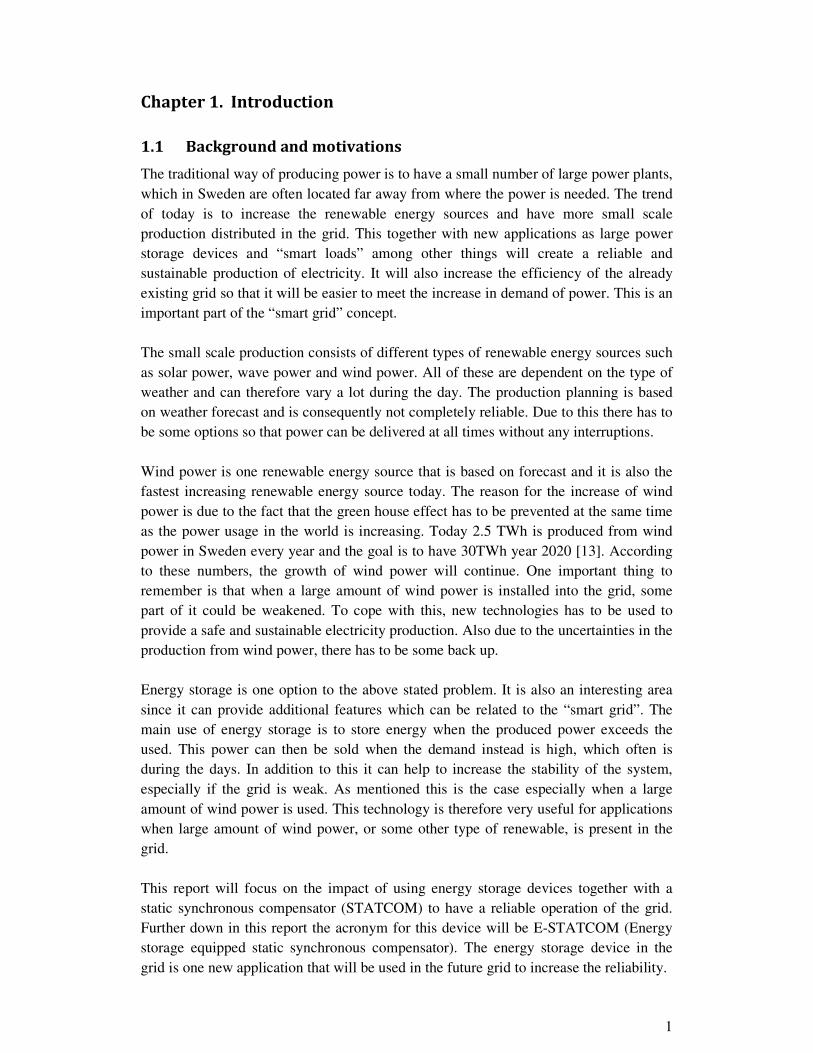
To decrease the simulation time and to have a smoother output of the measured quantities some simplifications has been done. One simplification done is to represent the full bridge converter with three ideal voltage sources, Fig.5. If this is done no PWM pattern is needed and the output will be smoother since there will be no ripple from the switching of the transistors. Notice that the ripple has almost the same frequency as the switching frequency and will therefore not give any information loss since we are only interesting in slow variations in this report. Another difference between the real converter and the three ideal voltage sources is that the real model has some losses due to switching. This is however not taken into consideration in this master thesis.

7

Fig.5 Three ideal voltage sources representing the voltage sourced converter

The ideal voltage source can provide an infinite amount of energy and is therefore not a good representation of energy storage. How to make a simple battery to limit the amount of energy will be described further down in the project.

8

2.4 Control systems

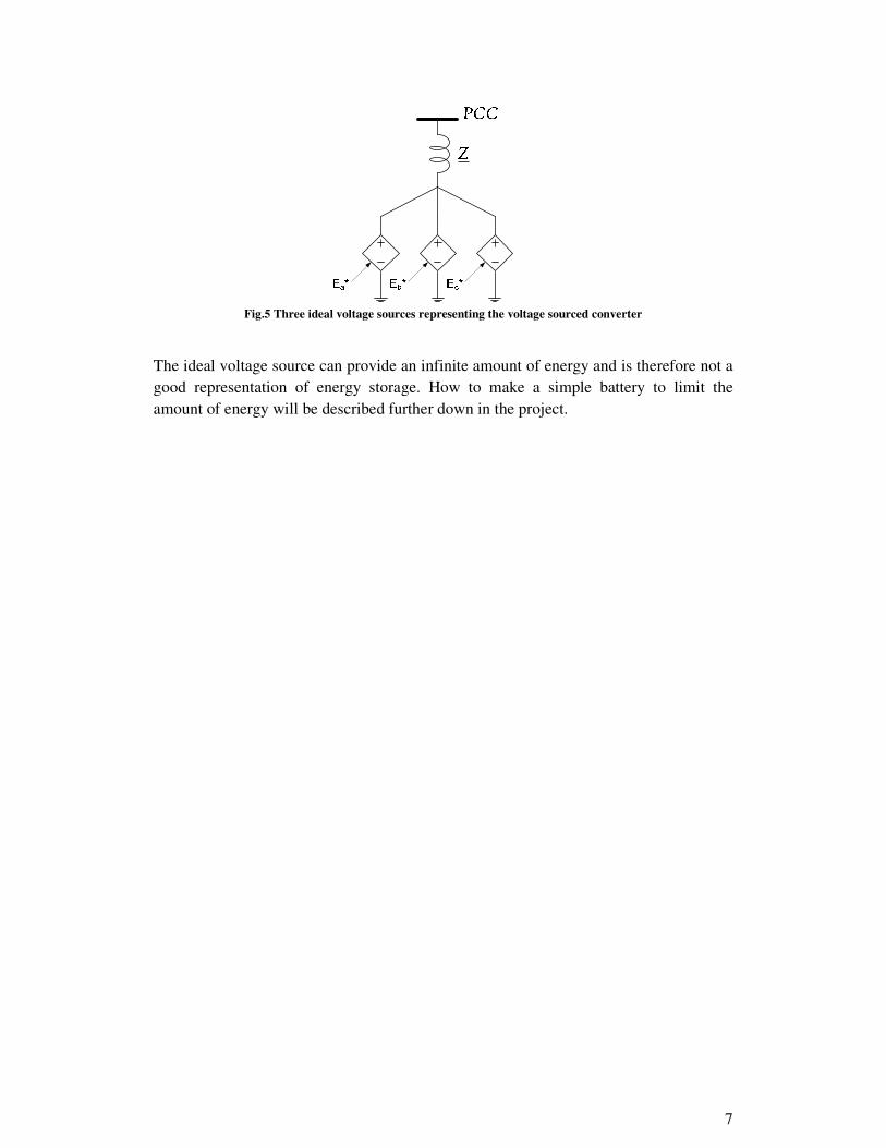
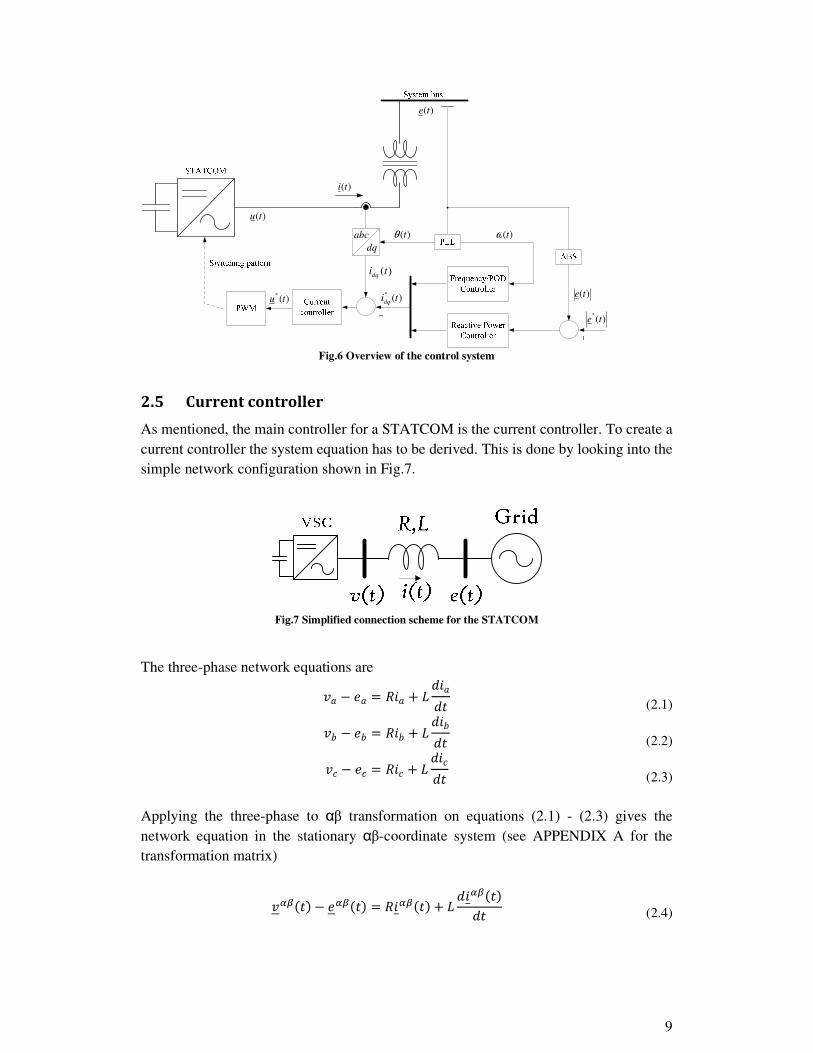
There are different control systems for the E-STATCOM where the main controller is the current controller. Besides this one additional control system is used to provide the reference current to the current controller. The most common additional used controller for a STATCOM is the voltage controller which controls the reactive power injection and absorption. This is used to regulate the voltage at the connection point of the STATCOM. The focus is however not on the voltage controller but instead on the frequency- and the power oscillation damping (POD) controller. An overview over the control system is given in Fig.6. Its operation can be described as follows. The voltage, e(t), at the system bus is measured to be sent to the Phase-Locked Loop (PLL) for angle estimation, also the absolute value of the voltage is taken to be compared with the reference voltage where the difference is sent to the reactive power controller for voltage control. The estimated angle is then used for transformation between the αβ-coordinate system and the dq-coordinate system. It is also used to provide the reference to the frequency controller. The reference current from the reactive power- and frequency/POD controllers are compared to the actual current of the system and this deviation is sent to the current controller which in turn sends the reference to the pulse width modulation (PWM) block that sets the switching pattern for the transistors in the converter. There is also one more controller that is used in a STATCOM and that is the DC voltage controller [18] which ensures that the DC-link voltage is kept constant. This controller is not shown in the figure for simplicity and it will not be treated in this report. Instead the focus will be on describing and deriving the current controller together with the frequency and POD controller. Notice also that all the controllers will be derived in the dq-system since the integral part of a PI controller can only be used when the quantities are in DC. It is also easier to compare the reference with the actual value if it is in DC compared to AC. The transformation matrix between three phase and dq can be found in APPENDIX A. Also to mention is that the system is voltage oriented so the d component corresponds to the active power and the q component is related to the reactive power.

9

)(tidq

)(*tidq

)(*te

)(*tu

)(te

)(ti

)(tu

)(te

abc

dq

)(tθ )(tω

Fig.6 Overview of the control system

2.5 Current controller

As mentioned, the main controller for a STATCOM is the current controller. To create a current controller the system equation has to be derived. This is done by looking into the simple network configuration shown in Fig.7.

Fig.7 Simplified connection scheme for the STATCOM

The three-phase network equations are

�� � �� � ��� � ��� (2.1)

�� � �� � ��� � ��� (2.2)

� � � � �� � � � (2.3)

Applying the three-phase to αβ transformation on equations (2.1) - (2.3) gives the network equation in the stationary αβ-coordinate system (see APPENDIX A for the transformation matrix)

������ � ������ � ������� � ������� (2.4)

10

Continuing by applying the αβ to dq-system transformation from APPENDIX A, the network equation instead looks like: [2]

��� � ��� � ���� � ����� � ��� (2.5)

The last part, ωLi

dq, in this equation comes from the transformation between αβ to dq coordinate system. The aim is to control the active and reactive power separately which is done by controlling the d component, which is related to the active power, and the q component, which is related to the reactive power, separately. This statement holds for a voltage oriented system where the d component is aligned with the voltage vector. In order to achieve this (2.5) have to be separated into a real and imaginary part and the following equations hold:

�� � �� � ��� � ��� � ��� (2.6)

�� � �� � ��� � ��� � ��� (2.7)

Fig.8 Block diagram over the current controller and the electrical system

Fig.8 shows a block scheme over (2.5). Ge(s) is the electrical system described by the right hand side of (2.5) and Fc(s) is the current controller. If the transfer function is calculated from the voltage error ∆v

dq to the current idq then it can be seen that it is a first order system described by (2.8)

����� � 1� � � � ��

(2.8)

jωL is the cross-coupling from the transformation mentioned above. As can be seen in (2.6) and (2.7) this cross-coupling term introduce a q-current dependency in (2.6) and a d-current dependency in (2.7). This will yield that a change in one of the d or q components will affect the other. This is not wanted since the aim is to control them separately. It is however removed in (2.8) by using feedback of the current through jωL, as shown in Fig.8. The equation will then be reduced to

11

������ � 1� � �

(2.9)

The current controller, Fc(s), can be described by the following equation

����� � ��� � � �� (2.10)

One way to calculate the control parameters is to look at the transfer function calculated from idq* to idq in Fig.8 and set it equal to a first order filter as in (2.11). A first order filter is chosen based on that the electrical system is a first order system and that a step response should follow the reference without any overshoot. The bandwidth (αcc) of the current controller can be decided according to how fast the control system should be.

�!��� � �����������1 � ����������� � "��� � "��

(2.11)

If the above equations are used it can be seen that the control parameters can be calculated as the following equations [2] ��� � "��

(2.12)

� � � "���

(2.13)

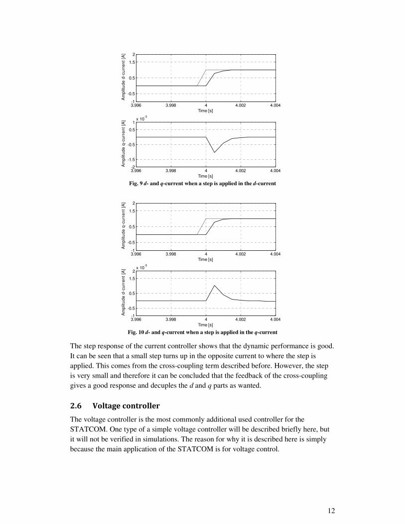
The following graph shows the behaviour of the current controller, derived with the above equations, when a step is applied. The bandwidth is chosen to be 500 Hz in this case. This is done in PSCAD in a system representing Fig.7. The reference to the controller will later on come from the frequency controller. It can be validated from the Fig.9 that the bandwidth of the current controller is 500 Hz by looking at the current rise-time which is the time it takes between 10-90% of the final value.

"�� � ln 9�& !�

trise is the rise time of the step response.

12

Fig. 9 d- and q-current when a step is applied in the d-current

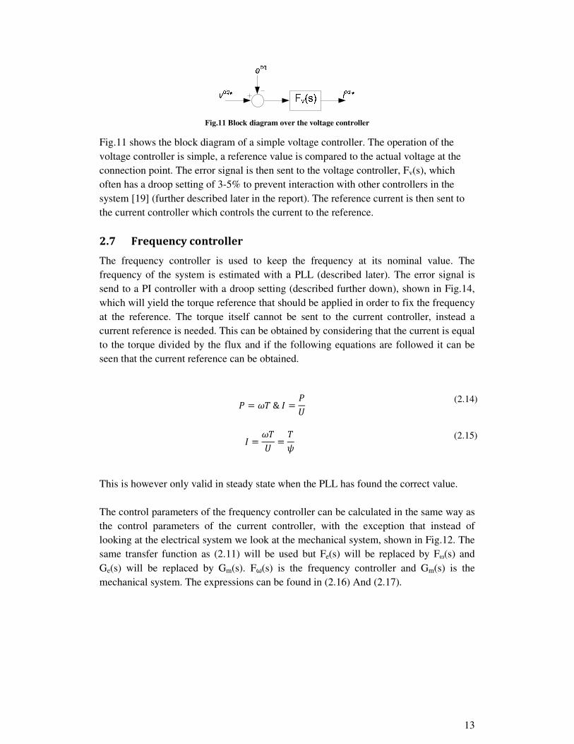
Fig. 10 d- and q-current when a step is applied in the q-current

The step response of the current controller shows that the dynamic performance is good. It can be seen that a small step turns up in the opposite current to where the step is applied. This comes from the cross-coupling term described before. However, the step is very small and therefore it can be concluded that the feedback of the cross-coupling gives a good response and decuples the d and q parts as wanted.

2.6 Voltage controller

The voltage controller is the most commonly additional used controller for the STATCOM. One type of a simple voltage controller will be described briefly here, but it will not be verified in simulations. The reason for why it is described here is simply because the main application of the STATCOM is for voltage control.

3.996 3.998 4 4.002 4.004-1

-0.5

0.5

1.5

2

Am

plit

ud

e d

-cu

rre

nt

[A]

Time [s]

3.996 3.998 4 4.002 4.004-2

-1.5

-0.5

0.5

1x 10

-3

Am

plit

ud

e q

-cu

rre

nt

[A]

Time [s]

3.996 3.998 4 4.002 4.004-1

-0.5

0.5

1.5

2

Am

plit

ud

e q

-cu

rre

nt

[A]

Time [s]

3.996 3.998 4 4.002 4.004-1

-0.5

0.5

1.5

2x 10

-3

Am

plit

ud

e d

-cu

rre

nt

[A]

Time [s]

13

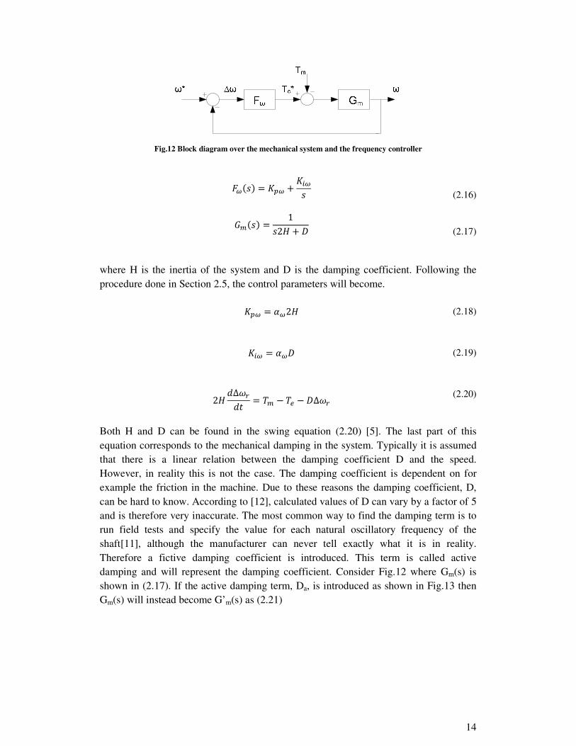
Fig.11 Block diagram over the voltage controller

Fig.11 shows the block diagram of a simple voltage controller. The operation of the voltage controller is simple, a reference value is compared to the actual voltage at the connection point. The error signal is then sent to the voltage controller, Fv(s), which often has a droop setting of 3-5% to prevent interaction with other controllers in the system [19] (further described later in the report). The reference current is then sent to the current controller which controls the current to the reference.

2.7 Frequency controller

The frequency controller is used to keep the frequency at its nominal value. The frequency of the system is estimated with a PLL (described later). The error signal is send to a PI controller with a droop setting (described further down), shown in Fig.14, which will yield the torque reference that should be applied in order to fix the frequency at the reference. The torque itself cannot be sent to the current controller, instead a current reference is needed. This can be obtained by considering that the current is equal to the torque divided by the flux and if the following equations are followed it can be seen that the current reference can be obtained.

' � �( & + � ',

(2.14)

+ � �(, � (- (2.15)

This is however only valid in steady state when the PLL has found the correct value. The control parameters of the frequency controller can be calculated in the same way as the control parameters of the current controller, with the exception that instead of looking at the electrical system we look at the mechanical system, shown in Fig.12. The same transfer function as (2.11) will be used but Fe(s) will be replaced by Fω(s) and Ge(s) will be replaced by Gm(s). Fω(s) is the frequency controller and Gm(s) is the mechanical system. The expressions can be found in (2.16) And (2.17).

14

Fig.12 Block diagram over the mechanical system and the frequency controller

�.��� � ��. � � .�

(2.16)

�/��� � 1�21 � 2

(2.17)

where H is the inertia of the system and D is the damping coefficient. Following the procedure done in Section 2.5, the control parameters will become. ��. � ".21

(2.18)

� . � ".2 (2.19)

21 ∆�&� � (/ � (� � 2∆�&

(2.20)

Both H and D can be found in the swing equation (2.20) [5]. The last part of this equation corresponds to the mechanical damping in the system. Typically it is assumed that there is a linear relation between the damping coefficient D and the speed. However, in reality this is not the case. The damping coefficient is dependent on for example the friction in the machine. Due to these reasons the damping coefficient, D, can be hard to know. According to [12], calculated values of D can vary by a factor of 5 and is therefore very inaccurate. The most common way to find the damping term is to run field tests and specify the value for each natural oscillatory frequency of the shaft[11], although the manufacturer can never tell exactly what it is in reality. Therefore a fictive damping coefficient is introduced. This term is called active damping and will represent the damping coefficient. Consider Fig.12 where Gm(s) is shown in (2.17). If the active damping term, Da, is introduced as shown in Fig.13 then Gm(s) will instead become G’m(s) as (2.21)

15

Fig.13 Block diagram over the mechanical system and the frequency controller with active damping

��/��� � 1�21 � 2 � 24

(2.21)

If the inner feedback loop is made as fast as the closed loop system the following hold: [2]. 2 � 2421 � "/

(2.22)

From (2.22) the total damping, D+Da, can be calculated based on the bandwidth and the inertia constant. The constant D does not necessarily have to be known, instead the sum of D+Da will be used.

2.7.1 Droop

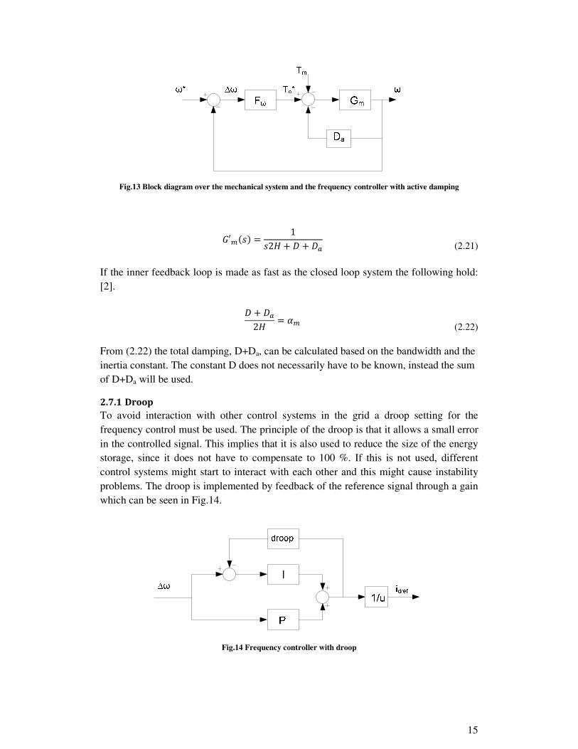
To avoid interaction with other control systems in the grid a droop setting for the frequency control must be used. The principle of the droop is that it allows a small error in the controlled signal. This implies that it is also used to reduce the size of the energy storage, since it does not have to compensate to 100 %. If this is not used, different control systems might start to interact with each other and this might cause instability problems. The droop is implemented by feedback of the reference signal through a gain which can be seen in Fig.14.

Fig.14 Frequency controller with droop

16

The error becomes higher if the droop percentage is increased which is seen in Fig.15. It can be seen that for zero droop the error is set to zero so that the frequency returns to its rated value of 50 Hz. The droop is then increased with one percentage each step up o a total of five percent. How large the deviation will be for each percent depends on the grid. Therefore the droop percentage will be individually decided from grid to grid according to the grid code shown in Fig.16 [7]

Fig.15 Frequency respons with droop setting

Fig.16 Grid Code

Fig.16 shows the grid code that is valid for the Nordic countries. It shows that if the voltage is between 0.9 and 1.05 p.u then the frequency should stay between 49 and 50.3 Hz for continuous operation, field A. If it is outside A then other actions has to be taken which will not be described any further here. If it is of interest more of this can be found in [7].

2.8 Power oscillation damping controller

Besides the frequency control the E-STATCOM can also be used for damping of mechanical oscillations that can occur in the grid due to different reasons, for example a

10 12 14 16

49.6

49.8

50

Fre

quency [

Hz]

Time [s]

17

fast load change or grid faults. Power oscillation damping can be achieved by either reactive or active power or both at the same time. The procedure is to inject or absorb power with the opposite sign of the oscillation of the rotor to force it to fade away. It has been shown that active power is more effective to damp power oscillations compared to use of only reactive power [16]. One explanation to this is that with reactive power the voltage is modulated to damp the oscillations and if too much reactive power is injected then the voltage will vary more than is allowed. If instead active power is used the voltage will not change in a lossless system and therefore much more active power can be injected and hence dampen the oscillations better. It will be shown further down in the report that the connection point of the compensator is also important when it comes to power oscillation damping. The most common way to find the reference signal for power oscillation damping is to look at the derivative of the variation of transmitted active power, since it will oscillate together with the rotor. This statement can be verified by linearizing (2.23)

' � �5�67 sin :

(2.23)

This is the power equation that shows how much power that can be transmitted between the two voltages V1 and V2 with the impedance X in between, δ is the power angle. If (2.23) is linearized with δ=δ0+∆δ then the equation becomes

∆' � �5�67 cos�:=� ∆:

(2.24)

If the derivative of the variations of transmitted power is taken it can be seen that it is related to the rotor speed ∆'� � �5�67 cos�:=� ∆:� � �5�67 cos�:=� ∆�

(2.25)

Another way is to measure the rotor angle directly, although this approach is not frequently used in reality since the rotor is often located too far away. The variation of the derivative of the voltage can also be used as a reference. This signal can be estimated with a newly proposed method called AN-PLL (Auto- Normalizing Phase Locked Loop) [15]. This method will be described later on in the report. If the oscillation of the rotor is known the way to proceed is to inject or absorb active power with the opposite sign compared to the oscillation. If the control system is designed in a proper way the power oscillations can be damped very fast, depending on how large the energy storage is. The damping controller is a pure proportional gain where the gain is set equal to the one calculated for the proportional part of the frequency controller.

18

Fig.17 Power oscillation damping controller

2.9 Modeling of Energy Storage

Different aspects can be taken into consideration when the size of the energy storage is designed. The size depends on what the E-STATCOM is going to be used for since it can be varied to suit different applications. If the application is to provide active power during islanding mode then the size of the energy storage should be large enough to supply the whole load with power. Depending on the size of the load this could be a huge amount of energy and therefore it is not feasible to use for larger applications. Another aspect is to design the energy storage so that it can store energy from wind farms when they supply energy and then this energy could be used when there is a lack of wind power. As a supplementary application it could be controlled so that the system can enter islanding mode if the load requires the same amount of power as the energy storage can provide. According to the above mentioned it is hard to decide on how large the energy storage should be and therefore it is needed to design the size individually for each project and according to the applications of the E-STATCOM.

To provide a limitation in the amount of energy and to have a simple representation of a battery a High-Pass (HP) filter is used. This filter is inserted in the reference current from the frequency controller, which can be seen in Fig.18 where the HP filter is inside the dotted box. The step response of a HP filter is shown in Fig.19 which shows that the reference current will be at its maximum in the beginning and hence full power will be delivered. As the curve decays the current will also decay and consequently also the amount of power that will be injected from the E-STATCOM. The decay will therefore represent the discharge of a battery and the size of the battery will be dependent on the time constant for the HP filter. The time constant can be changed to fit the amount of time the battery should last.

Fig.18 Overview of the control system with a HP-filter as battery representation

19

Fig.19 Step response of a HP filter

2.10 Synchronization system

When connecting a STATCOM to the grid it first has to be synchronized with the grid frequency. It will be described in this chapter how to track the frequency of the system so that the synchronization can be performed. The information about the grid frequency is then further used to control the frequency and to give the transformation angle for the αβ to dq-transformation. This can be done with a conventional Phase-Locked Loop (PLL) or with a newly proposed approach called Auto-Normalizing Phase-Locked Loop (AN-PLL). In addition to frequency tracking it will be described how the AN-PLL can be used to find the reference for power oscillation damping.

2.10.1 Traditional Phase-Locked Loop (PLL)

The most common used method for tracking frequency variations is to use a PLL. It is a well known method that shows good performance, especially when the STATCOM is connected to a strong grid where the voltage amplitude is fixed. Mathematically the PLL can be described as [15] �>? ��� � @5A���

(2.26)

BC?��� � ���� � @6A���

(2.27)

where k1 and k2 are the control parameters and the error signal is

A��� � �D�EF���������G�� � ��,������

(2.28)

0 200 400 600 800 1000 1200 1400 1600 18000

0.1

0.2

0.3

0.4

0.5

0.6

0.7

0.8

0.9

1Step Response

Time (sec)

Am

plit

ude

20

Vp is the voltage amplitude of the positive sequence and vpdq (t) is the positive sequence

of the grid voltage. �> is the speed estimate and BC is the position estimate. (2.18) and (2.19) says that the speed estimate is updated proportionally to the error signal and the position estimate is updated as the integral of the speed estimate with a correction factor [2]. According to (2.28) vp,q(t) should be zero so that the error is zero. It can be seen that the parameters are dependent on the voltage amplitude Vp, and therefore the voltage amplitude does not affect the signals when connected to a strong grid, since the voltage is fixed in that case. If instead the STATCOM is connected to a weaker grid then the voltage amplitude variations could cause the bandwidth of the PLL to change due to the described voltage amplitude dependency. The solution to this problem could be to use the AN-PLL [15].

∫

∫

( )tθ̂ ( )tε ( )tω

( ) )(tvαβ ( ) )(tv

dq

( ) )(tvdq

ofs

( ) )(tvdq

n

( ) )(tvdq

p

)(, tv qp

)(, tv dp

pV1

Fig. 20 Phase-Locked Loop

2.10.2 Auto-Normalizing Phase-Locked Loop (AN-PLL)

Compared to the regular PLL the AN-PLL utilizes all the information about the complex voltage, not only the argument, by using the complex logarithm [15] logJ�K � logJL�LK � � argJ�K

(2.29)

)(te η−( ) )(tv norm

αβ( ) )(tvαβ ( ) )(tv

dq

norm

( ) )(, tvdq

normp

∫

∫

Fig.21 Block diagram of the AN-PLL

Consider Fig.21 which shows the block diagram over the AN-PLL. The logarithm is applied to the estimated positive sequence of the complex voltage. This signal is divided into two parts as (2.29) and each part is sent to a PI-regulator where the output is shown in (2.30) and (2.31).

21

O��� � @� log PQ�����QR � @ S log PQ���T�QRTUVW

(2.30)

���� � @� arg PQ�����QR � @ S arg PQ���T�QR TUVW

(2.31)

This will yield the variations of the derivative of the voltage (2.30) and the estimated angular frequency (2.31). These are integrated to give the grid voltage angle, (2.33), and a scaling factor, (2.32), that normalizes the voltage vector to unity. [15]

X��� � S O�T�TUVW

(2.32)

B��� � S ��T�TUVW

(2.33)

From (2.30) to (2.33) it can be seen that all the needed signals are estimated. (2.30) gives the reference signal to the power oscillation damping controller, (2.31) gives the reference to the frequency controller and (2.33) gives the transformation angle used in the αβ- to dq-transformation. The additional properties makes the AN-PLL much more reliable in this report since it increases the stability when connected to weak grids and also because it gives a signal that can be used for power oscillation damping. Further information can be found in [15].

22

23

Chapter 3. Power oscillation damping

As mentioned earlier the principle of damping power oscillations is to either inject or absorb power with the opposite sign compared to the oscillations. It was also mentioned that the efficiency of damping oscillations is dependent on the connection point of the compensator. In this chapter this statements will be described and shown by changing the location of connection of the E-STATCOM. Also mathematical calculations will be done to verify the simulation and to show that it is possible to increase the stability by connecting an E-STATCOM.

3.1 Analytical investigation

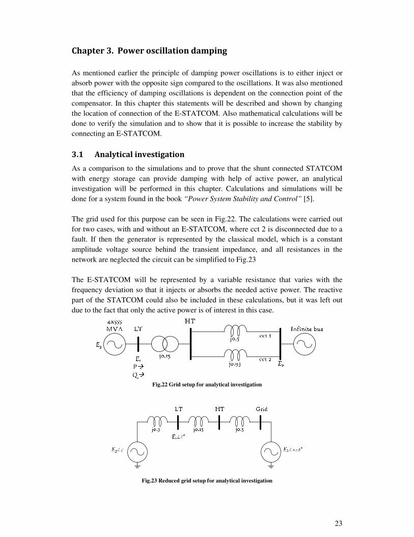
As a comparison to the simulations and to prove that the shunt connected STATCOM with energy storage can provide damping with help of active power, an analytical investigation will be performed in this chapter. Calculations and simulations will be done for a system found in the book “Power System Stability and Control” [5]. The grid used for this purpose can be seen in Fig.22. The calculations were carried out for two cases, with and without an E-STATCOM, where cct 2 is disconnected due to a fault. If then the generator is represented by the classical model, which is a constant amplitude voltage source behind the transient impedance, and all resistances in the network are neglected the circuit can be simplified to Fig.23 The E-STATCOM will be represented by a variable resistance that varies with the frequency deviation so that it injects or absorbs the needed active power. The reactive part of the STATCOM could also be included in these calculations, but it was left out due to the fact that only the active power is of interest in this case.

Fig.22 Grid setup for analytical investigation

Fig.23 Reduced grid setup for analytical investigation

24

3.1.1 Small signal stability without E-STATCOM

To analyze the small-signal stability characteristics of the system at a steady-state condition following a transient, the system has to be linearized around an initial operating point [5]. The parameters used are listed and described below KS = synchronizing torque coefficient in pu torque/rad KD = Damping torque coefficient in pu torque/pu speed deviation H = Inertia constant in MW*s/MVA ω0 = Rated speed in elec.rad/s ∆ωr = Per unit speed deviation δ = Rotor angle in elec.rad Tm = Mechanical torque in per unit Te = Electrical torque in per unit Eg = Voltage amplitude at generator in per unit Eb = Voltage amplitude at infinite bus in per unit Et = Voltage amplitude at low voltage side of the transformer in per unit XT = Total impedance of the grid in per unit Table 1 Table of parameters

Consider Fig.23, if Eg is used as reference then the current is

+YZ � [Y � [\�cos : � � sin :��7]

(3.1)

And the complex power is

^_ � ' � �` � [a+bZ � [\ sin :7] � � [YJ[Y � [\ cos :K7]

(3.2)

In per unit the active power is equal to the torque and hence becomes [5]

(� � '� � [Y[\7] sin :

(3.3)

Linearizing this equation with δ=δ0+∆δ gives

∆(� � [Y[\7] cos := �∆:�

(3.4)

Let

�! � [Y[\7] cos :=

(3.5)

The equations of motion in per unit are

25

∆�&� � 121 �(/ � (� � �c∆�&�

(3.6)

� ∆�& � �=∆�&

(3.7)

If these two equations are linearized the following is obtained ∆�&� � 121 �∆(/ � �d∆: � �c∆�&�

(3.8)

∆:� � �=∆�&

(3.9)

Written in state space form we get � e∆�&∆: f � g� �c21 � �d21�= 0 i e∆�&∆: f � g 1210 i∆(/

(3.10)

From the linearization the following characteristic equation will be found

j6 � �c21 j � �d�=21

(3.11)

Which is of the same form as: j6 � 2O�kj � �k6

(3.12)

If (3.11) is set equal to (3.12) then it can be seen that the natural frequency of the oscillations is

�k � l�d�=21

(3.13)

The damping ratio is

O � �c41�k

(3.14)

The eigenvalues are j5, j6 � �O�k n �ko1 � O6

(3.15)

26

The damped frequency is �� � �ko1 � O6

(3.16)

3.1.2 Small signal stability with E-STATCOM

Fig.24 Grid system with shunt compensation

In the case when the E-STATCOM is connected, Fig.24, the electrical torque will be different and hence also the synchronizing torque coefficient KS. The derivation of the expression for the generator power in this case is extensive and will not be done here, if it is of further interest it can be found in [6]. The final expression for the generator power becomes '�:� p � sin : � ��O � cos :�7dqr�!s � �� sin :�7dqrt!s

(3.17)

Where � � [Y�! J7Y � 7!K⁄ and O � J[Y �!⁄ KJ7! 7Y⁄ K and XSHC is the short-circuit

reactance of the system, seen from the connection point of the E-STATCOM. Bsh is the susceptance representing the reactive part of the E-STATCOM but in this specific case where only the active power of the E-STATCOM is investigated, Bsh is set to zero and hence the last part in the above equation is neglected. As mentioned the E-STATCOM is represented by a resistance that varies with the frequency. The expression can be seen in (3.18) �!s � ��c!U4U�v/∆�

(3.18)

Gsh is the conductance representing the E-STATCOM, KDstatcom is the proportional gain in the power oscillation damping controller. It has been stated that the injection or absorption should have the opposite sign to the oscillation of the rotor, therefore a minus sign has to be used in (3.18) since otherwise it will increase the oscillations. To find KS, (3.17) has to be linearized so that the above described state space matrix can be used. This linearization is performed in Wolfram Mathematica which allows non-numerical calculations and the result is given in state space form according to (3.19) � e∆�&∆: f � e�55 �56�65 �66f e∆�&∆: f � w�55�65x ∆(/

(3.19)

27

�55 � �2 � � b �c!U4U�v/ b 7dqr�O � cos :=�21

(3.20)

�56 � �� cos :=21

(3.21)

�65 � �=

(3.22)

�66 � 0

(3.23)

If equation (3.20) is compared with a11 in (3.10) then it can be seen that the damping coefficient KD contains two parts. The first part is the natural damping, D, of the system and the second part comes from the E-STATCOM.

3.1.3 Comparison with and without E-STATCOM

The eigenvalues shows where the pole pair of the system is located and this can give information about the stability of the system. If the pole pair is located on the right side of the imaginary axis then the system will be unstable. If they are located on the imaginary axis then the system will not be unstable but it also not damped, so an oscillation will be sustained. In order to have a stable system then the pole pairs have to be located on the left side of the imaginary axis. P = 0.9 Q = 0.3 Et = 1—36° Eb = 0.995∠0° H=3.5 MW*s/MVA Table 2 Initial values for mathematical calculations

If the previous mathematical calculations are performed for the examples shown in Fig.23 and Fig.24 with the initial conditions (in p.u) shown in Table 2, and with the impedance values in Fig.23, the following results will be found. Uncompensated E-STATCOM KD 0 -12.468 Eigenvalues λ 0±j5.8304 -0.4708±j5.8114 Damped frequency ωd 0.9279 Hz 0.9249 Hz Damping ratio ξ 0 0.112 Undamped natural frequency ωn 0.9279 Hz 0.9279 Hz Table 3 Results for calculations

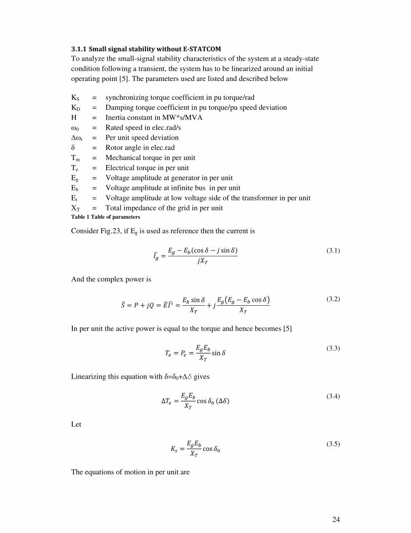
In the uncompensated case the eigenvalues are located on the imaginary axis and therefore the system is not unstable but also not damped. If the eigenvalues are plotted, Fig.25, it can be seen that the pole pairs have moved into the left half plane. Now the system is damped and the stability has increased.

28

Fig.25 Pole-pair locations

3.2 Simulations on power oscillation damping

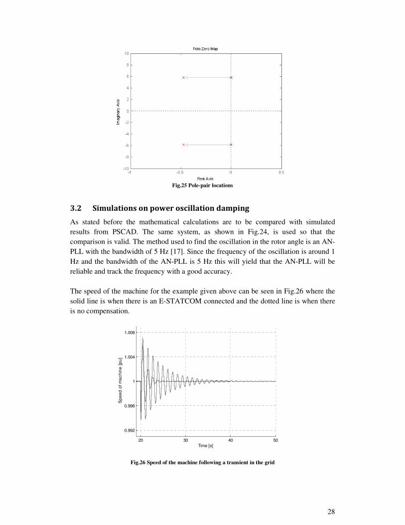
As stated before the mathematical calculations are to be compared with simulated results from PSCAD. The same system, as shown in Fig.24, is used so that the comparison is valid. The method used to find the oscillation in the rotor angle is an AN-PLL with the bandwidth of 5 Hz [17]. Since the frequency of the oscillation is around 1 Hz and the bandwidth of the AN-PLL is 5 Hz this will yield that the AN-PLL will be reliable and track the frequency with a good accuracy. The speed of the machine for the example given above can be seen in Fig.26 where the solid line is when there is an E-STATCOM connected and the dotted line is when there is no compensation.

Fig.26 Speed of the machine following a transient in the grid

20 30 40 50

0.992

0.996

1

1.004

1.008

Time [s]

Sp

ee

d o

f m

ach

ine

[p

u]

29

It can be seen in Fig.26 that the damping of oscillations is improved when an E-STATCOM is connected, represented by the solid line. According to the pole pairs shown in Fig.25 the uncompensated grid should not be damped at all although that it can be seen in the figure that the dotted curve is damped. The reason for this is that in the mathematical calculations it is assumed that there is no resistance in the grid and that the machine is represented by the classical model, which is a simplification. In this case there will be no damping. In the simulation on the other hand a complete model of the machine is used and not represented by the classical model. In this model the flux tries to stay constant and therefore during the oscillation it will try to oppose the oscillation and the flux will slowly change [5]. This will cause the oscillations to be damped and in addition to this, one damping winding can be found in the machine. The damping winding will provide damping at lower frequencies, and since the frequency of the oscillation is around 1 Hz this will be affected by the damping winding. The important thing to notice when comparing the mathematical calculations with the simulated result is that the frequency of the oscillation is the same in both cases. Both results also prove that an E-STATCOM will provide damping to the system. Notice that they can never show exactly the same result when simplifications are made in the mathematical expressions, but a hint that both shows that the stability is improved is given.

3.3 Impact on PCC for power oscillation damping

The point of connection is important for frequency control but even more important when it comes to power oscillation damping. This can be seen in (3.17) where the two terms XSHC and ξ change depending on where the connection point is located. The E-STATCOM will provide larger damping if it is connected closer to the generator. The explanation for this is that if the connection point is close to the infinite bus then nearly all of the injected current will go into the this bus, due to the lower impedance, and affect the oscillation very little. If the connection point is moved closer to the generator then the damping will increase due to that more and more of the injected current will aid in damping the oscillation. Fig.28 shows the difference in damping when the connection point is changed. The grid used is the same as for the example above, and the different locations of the connection point can be seen in Fig.27.

Fig.27 Connection points of the E-STATCOM

30

Fig.28 Speed of the machine following a transient in the grid for different connection points

It can be seen in Fig.28 that the damping increases as the connection point moves closer towards the generator. This can also be validated with mathematical calculations by looking at the pole pair location. This is realised in Fig.29 where it can be seen that the stability has increased since the pole pair moves from the imaginary axis further into the left half plane as the connection point is moved.

Fig.29 Pole-pair location for different connection point of the E-STATCOM

20 30 40

0.992

0.996

1

1.004

1.008

Speed o

f m

achin

e [

pu]

Time [s]

No Damping

Damping LT

Damping HT

31

Chapter 4. Simulation results

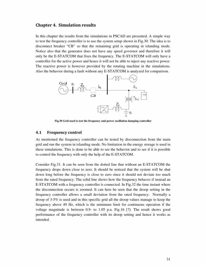
In this chapter the results from the simulations in PSCAD are presented. A simple way to test the frequency controller is to use the system setup shown in Fig.30. The idea is to disconnect breaker “CB” so that the remaining grid is operating in islanding mode. Notice also that the generator does not have any speed governor and therefore it will only be the E-STATCOM that fixes the frequency. The E-STATCOM will only have a controller for the active power and hence it will not be able to inject any reactive power. The reactive power is however provided by the rotating machine in the simulations. Also the behavior during a fault without any E-STATCOM is analyzed for comparison.

Fig.30 Grid used to test the frequency and power oscillation damping controller

4.1 Frequency control

As mentioned the frequency controller can be tested by disconnection from the main grid and run the system in islanding mode. No limitation in the energy storage is used in these simulations. This is done to be able to see the behavior and to see if it is possible to control the frequency with only the help of the E-STATCOM. Consider Fig.31. It can be seen from the dotted line that without an E-STATCOM the frequency drops down close to zero. It should be noticed that the system will be shut down long before the frequency is close to zero since it should not deviate too much from the rated frequency. The solid line shows how the frequency behaves if instead an E-STATCOM with a frequency controller is connected. In Fig.32 the time instant where the disconnection occurs is zoomed. It can here be seen that the droop setting in the frequency controller allows a small deviation from the rated frequency. Normally a droop of 3-5% is used and in this specific grid all the droop values manage to keep the frequency above 49 Hz, which is the minimum limit for continuous operation if the voltage magnitude is between 0.9- to 1.05 p.u. Fig.16 [7]. The result shows good performance of the frequency controller with its droop setting and hence it works as intended.

32

Fig.31 Frequency behaviour during system islanding. Dotted = without compensation, Solid = with

compensation

Fig.32 Zoom from Fig.29

10 20 30

10

30

50

Fre

qu

en

cy [

Hz]

Time [s]

2 3 4 5 6

49.2

49.6

50

Time [s]

Fre

qu

en

cy [

Hz]

33

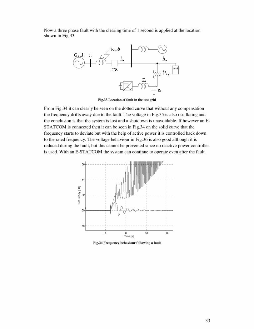
Now a three phase fault with the clearing time of 1 second is applied at the location shown in Fig.33

Fig.33 Location of fault in the test grid

From Fig.34 it can clearly be seen on the dotted curve that without any compensation the frequency drifts away due to the fault. The voltage in Fig.35 is also oscillating and the conclusion is that the system is lost and a shutdown is unavoidable. If however an E-STATCOM is connected then it can be seen in Fig.34 on the solid curve that the frequency starts to deviate but with the help of active power it is controlled back down to the rated frequency. The voltage behaviour in Fig.36 is also good although it is reduced during the fault, but this cannot be prevented since no reactive power controller is used. With an E-STATCOM the system can continue to operate even after the fault.

Fig.34 Frequency behaviour following a fault

4 8 12 16

48

50

52

54

56

Time [s]

Fre

qu

en

cy [

Hz]

34

Fig.35 Voltage behaviour without E-STATCOM

Fig.36 Voltage behaviour with E-STATCOM

5 6 7 8

-30

0

30

Time [s]

Vo

lta

ge

at

PC

C [

kV

]

5 7 9 11

-30

0

30

Time [s]

Vo

lta

ge

at

PC

C [

kV

]

35

4.2 Power oscillation damping

It has been shown in Chapter 3 that the E-STATCOM can provide active damping by injecting or absorbing active power. Furthermore, in Section 3.3, it has been shown that the location of the compensator has a great impact on the ability of the system to provide effective damping to power oscillations. Also, different synchronization algorithms have been described and can be used to provide the needed signals to the damping controller. Here, the dynamic performance of the E-STATCOM when using AN-PLL for damping power oscillations in the transmission system is shown. In order to trigger a power oscillation, a step in the mechanical torque acting on the generator shaft in Fig.30 is applied. As a result, low frequency oscillation in the generator speed, resulting in oscillations in the transmitted power, will be excited, as shown in Fig.37 (dotted line). If the E-STATCOM is connected to the grid and active, the investigated control system will react to the oscillation and inject the needed active power in order to increase the system damping. This can be seen through the solid line in Fig.37, which shows the generator’s rotor speed when the compensator is active. From the comparison, ist is possible to observe that the E-STATCOM is capable to increase the system damping. The amount of damping that can be provided by the compensator, i.e. the time needed to cancel the oscillation, is dependent on the size of the energy storage (large storage would allow higher active power injection, thus fast damping action).

Fig.37 Speed of machine following a transient without compensation (dotted] and with compensation (solid)

20 22 24

0.992

0.996

1

1.004

1.008

Speed o

f m

achin

e [

pu]

Time [s]

36

37

Chapter 5. Falbygdens Energi AB

In this report the different applications for an E-STATCOM has been discussed. Also the different control system used in the E-STATCOM have been derived. Results from simulations have proven that the dynamic performance of the different controllers is good and that they function as intended. In this section the E-STATCOM with all the derived controllers will be tested in the grid of Falbygdens Energi AB (FEAB). The need for an E-STATCOM from a dynamical point of view during faults and other occasions will be evaluated. Also other applications will be taken into account. The short-circuit power of the system at the connection to the infinite bus is 179 MVA, which is ~11 times larger than the installed, 16MW, amount of wind power. This yields that the frequency probably will be fixed by the infinite source although that this might change if more wind power is installed.

5.1 Grid setup

A part of the grid in Falköping has been simplified and built in PSCAD. Since it is a simplification of the grid, one level above FEAB is not considered and is therefore represented by an infinite source behind an impedance that will represent the short-circuit power. The transformer between the infinite bus and busbar Norra is rated to 40MVA which brings down the short-circuit capacity to 179 MVA at busbar Norra. The load, which is considered to vary between 3.5-30 MVA with a power factor of 0.95, and two incoming cables are connected to this busbar. It is also to this bus that the E-STATCOM will be connected (in the simulations). The two incoming cables connect Norra with Östra and from that point one cable goes to the wind farm at Backgården and two cables to the wind farm at Källeberg. The wind farm at Backgården consists of three 2MW DFIG generators and at Källeberg there are five 2MW DFIG generators. A grid overview can be found in Fig.38

38

Fig.38 FEAB grid overview

5.2 Simulation results

Different simulations have been performed in the model of the FEAB grid to test if there is a need for an E-STATCOM from a dynamical point of view. The cases that have been performed can be seen in the table below. Type of occasion Location Additional information

3-phase fault Cable connecting Östra-Källeberg

Close to busbar Källeberg

3-phase fault Cable connecting Norra-Östra Middle of the cable Fluctuating wind power Not constant power Voltage dip Feeding grid 0.7 remaining voltage Islanding mode Connection to the main grid No connection to the main

grid Table 4

Notice that the power delivered from the two wind farms are set to be constant for all simulations except for when the power is fluctuating.

5.2.1 Three phase to ground fault & voltage dip

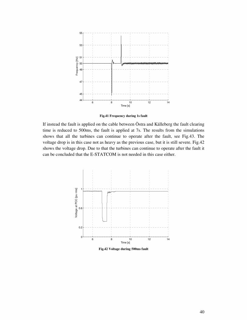
The most severe fault is three phase to ground since none of the phases can transmit power in this case. This is also the most common fault in FEAB grid since cables are used and if something happens to the cable it is most likely that it will affect all three phases. Due to these two reasons the faults applied in the simulations are chosen to be three phase to ground but with different locations in the grid. If a three phase to ground fault occurs in one of the two cables connecting busbar Norra with Östra, having a clearing time of 1s, a severe voltage drop with less than 0.2 p.u

39

remaining voltage will take place. This can be seen in Fig.39. The consequence is that the turbines at the wind farms will stall and a shutdown is unavoidable, which can be seen in Fig.40. The only thing that can be noticed in the frequency is the transient shown in Fig.41 but this is not serious since it recovers fast. The oscillations that can be seen after the fault comes from that the wind turbines are not disconnected in the simulation. In reality this will not be present since in that case the wind turbines will be disconnected. The same behavior can be seen in the voltage. Due to that there is no phase deviation the active power from the E-STATCOM is not needed when this type of fault occurs. The location of the E-STATCOM also prevents it from damping the oscillations of the rotor in the turbines, since most of the current from the E-STATCOM will flow into the main grid, due to the lower impedance. Reactive power injection might be beneficial to the system, although the majority of the injected reactive power will flow into the fault.

Fig.39 Voltage during 1s fault

Fig.40 Rotor speed in p.u during 1s fault

6 8 10 12 140

0.2

0.6

1

Time [s]

Voltage a

t P

CC

[pu r

ms]

6 8 10 12 140.5

1

1.5

2

Time [s]

Ro

tor

sp

ee

d [

pu

]

40

Fig.41 Frequency during 1s fault

If instead the fault is applied on the cable between Östra and Källeberg the fault clearing time is reduced to 500ms, the fault is applied at 7s. The results from the simulations shows that all the turbines can continue to operate after the fault, see Fig.43. The voltage drop is in this case not as heavy as the previous case, but it is still severe. Fig.42 shows the voltage drop. Due to that the turbines can continue to operate after the fault it can be concluded that the E-STATCOM is not needed in this case either.

Fig.42 Voltage during 500ms fault

6 8 10 12 1444

45

47

49

50

51

53

55

Time [s]

Fre

qu

en

cy [

Hz]

6 8 10 12 140

0.2

0.6

1

Time [s]

Vo

lta

ge

at

PC

C [

pu

rm

s]

41

Fig.43 Rotor speed in p.u during 500ms fault

A 0.7 p.u. remaining voltage dip has also been applied in the feeding grid with a fault clearing time of 300ms. All of the turbines continue to operate after the fault is cleared. One interesting use of the E-STATCOM could in this case be to compensate for the loss of active power during the fault. This however requires some other control schemes and is therefore not included in this report.

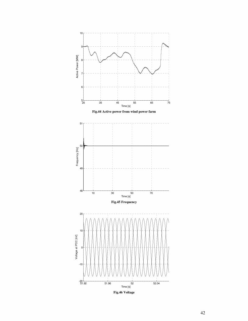
5.2.2 Fluctuating power from wind farms

The torque to the generators in the wind turbines has been constant during all the previous simulations. This means that the wind speed will put a constant force on the blades, which is not true in reality since the wind speed varies all the time. Therefore data from a real wind turbine has been used in one simulation to see if a more realistic wind speed would cause any problems with the voltage or the frequency at busbar Norra. The varying power from the wind farm can be seen in Fig.44. The load has in this case been reduced so that some of the power is fed into the infinite bus. The behaviour of the frequency and the voltage is found in Fig.45 and Fig.46. According to the figures there is no problem with the frequency or the voltage. As mentioned this is for the current case where 16 MW of wind power is installed in the grid with the short-circuit capacity of 179 MVA. In the future when the ratio between the short-circuit capacity and the amount of wind power decreases the results could be complete different.

6 8 10 12 140.5

1

1.5

2

Time [s]

Ro

tor

sp

ee

d [

pu

]

42

Fig.44 Active power from wind power farm

Fig.45 Frequency

Fig.46 Voltage

25 35 45 55 65 755

6

7

8

9

10

Active

Po

we

r [M

W]

Time [s]

10 30 50 7048

49

50

51

Time [s]

Fre

qu

en

cy [

Hz]

51.92 51.96 52 52.04-20

-10

0

10

20

Time [s]

Vo

lta

ge

at

PC

C [

kV

]

43

5.2.3 System islanding

As mentioned before the frequency controller is mostly needed in case of system islanding or if the network is very weak. To be able to operate in islanding mode is probably not the main driving force to install a STATCOM with energy storage, but if installed it can be used for this application. In this scenario the E-STATCOM can temporarily provide energy meanwhile other actions are taken in the local grid, for example the use of a “smart load”. The “smart load” adapts the load so that there is a power balance between the load and the generated power, in this case the power from the two wind farms. It will be shown, from simulations, that it is possible to run the system in islanding mode if an energy storage device is used and if it is large enough to supply the needed power. Examples over two different types of “smart load” will also be shown.

5.2.4 Islanding mode without “smart load”

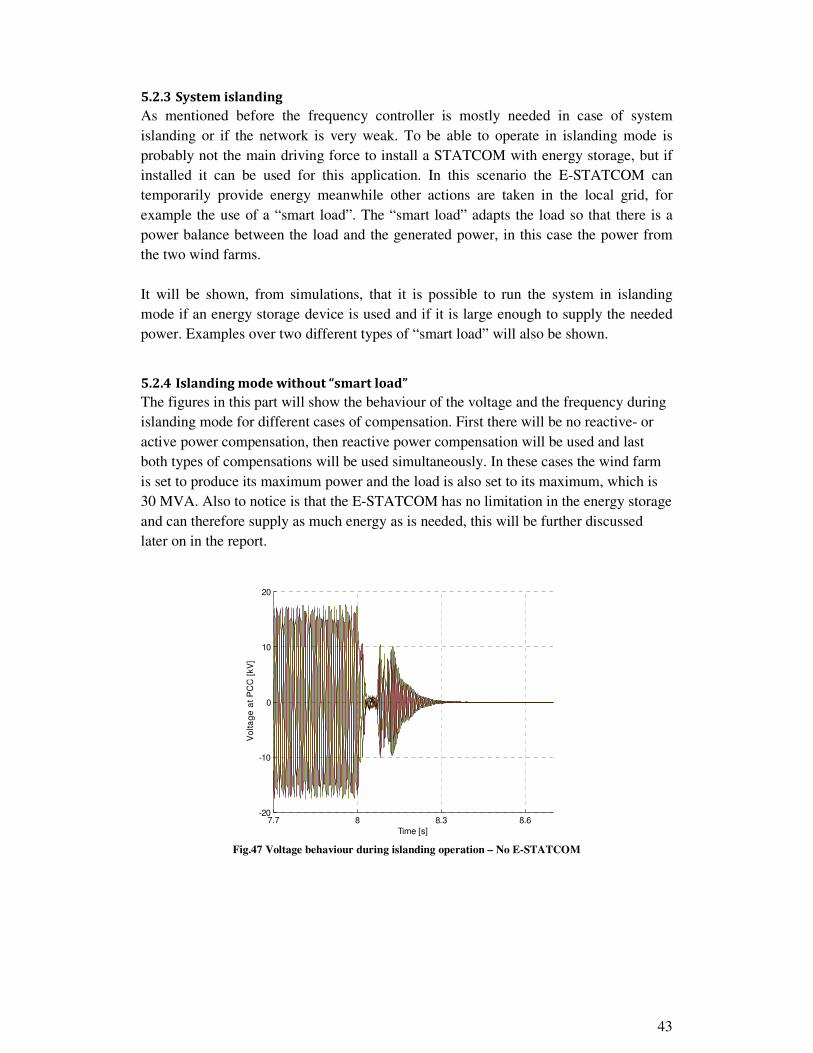
The figures in this part will show the behaviour of the voltage and the frequency during islanding mode for different cases of compensation. First there will be no reactive- or active power compensation, then reactive power compensation will be used and last both types of compensations will be used simultaneously. In these cases the wind farm is set to produce its maximum power and the load is also set to its maximum, which is 30 MVA. Also to notice is that the E-STATCOM has no limitation in the energy storage and can therefore supply as much energy as is needed, this will be further discussed later on in the report.

Fig.47 Voltage behaviour during islanding operation – No E-STATCOM

7.7 8 8.3 8.6-20

-10

0

10

20

Time [s]

Vo

lta

ge

at

PC

C [

kV

]

44

Fig.48 Frequency behaviour during islanding operation – No E-STATCOM

Fig.47 and Fig.48 show the voltage and frequency at busbar Norra when the system enters islanding mode at 8s, no compensation is used. It can be seen that the voltage drops down to zero within 300ms and that the frequency drifts away, hence the system is lost.

Fig.49 Voltage behaviour during islanding operation –Reactive power compensation

7 8 9 10

40

50

60

70

80

90

Time [s]

Fre

qu

en

cy [

Hz]

8 14 20-20

-10

0

10

20

Time [s]

Voltage a

t P

CC

[kV

]

45

Fig.50 Frequency behaviour during islanding mode – Reactive power compensation

Fig.49 and Fig.50 shows the behaviour when a simple reactive power controller is used. The voltage drops down to zero but it takes longer time than the previous example. The system is however lost in this case also.

Fig.51 Voltage behaviour during islanding mode – With E-STATCOM

4 8 12 16 20-30

-20

0

30

50

Time [s]

Fre

qu

en

cy [

Hz]

8 8.6 9.2 9.8-20

-10

0

10

20

Time [s]

Vo

lta

ge

at

PC

C [

kV

]

46

Fig.52 Frequency behaviour during islanding operation – With E-STATCOM

In Fig.51 and Fig.52 a STATCOM with energy storage capability is used and as can be seen the system is kept alive. The voltage behavior is now reduced to a small dip instead of dropping down to zero as shown in both previous cases. The frequency is also kept close to the rated frequency, it is only the droop that prevents it to reach the rated value. Due to these results it is proven that the dynamic performance of the frequency controller is very good and that is it possible to continue to operate in system islanding. The two wind farms produce 10 and 6 MW respectively in these simulations, which means that the E-STATCOM needs to inject 13 MW to meet the power demand during peak load. Therefore this case will not be true in reality since the limitation for the energy storage is set to be 2MW for 15 min in this investigation, which is set by ABB. The criteria for enter islanding mode is hence that the load should only require a maximum of 2 MW additional power on top of the power produced from the two wind farms. So in the case above where the wind farms produce 16 MW the maximum load for islanding mode is 18 MW. Notice that this is only feasible for 15 min. If instead the load requires less than the produced power, then the extra power can be used to charge the energy storage or in the worst case be wasted in the DC-chopper in the STATCOM. The frequency response will be the opposite in this case and will increase which can be seen in Fig.53.

8 14 20

48,5

49,5

50

50,5

Time [s]

Fre

qu

en

cy [

Hz]

47

Fig.53 Frequency behaviour if the produced power exceeds the load during islanding mode

5.2.5 Islanding mode with “smart load”

The limitation mentioned above implies that if 2 MW is injected from the E-STATCOM the operation time is limited to 15 min. To increase this time the load could be adapted to the produced wind power. In that case the frequency will be kept at the rated value without help from the E-STATCOM. The idea is to let the E-STATCOM compensate for the extra power needed directly when the islanding operation starts and then slowly reduce together with the load until the power from the load is equal or less to the produced power from the wind farm. Notice that the load cannot be perfectly matched to the produced power since it varies with the wind speed, which is not constant. Therefore there are two alternatives when matching the load to the wind power. Consider Fig.54 and assume that the power delivered by the wind farm is the same as shown in Fig.44, since the power from the wind farm fluctuates. One way is to put the load in the middle of the power curve and let the E-STATCOM inject or absorb power when it is needed to keep the power balance. Another scenario is instead to adapt the load so that it is slightly beneath the fluctuating power from the wind farm, which is represented by the lowest curve in Fig.54. The extra power from the wind farm can be either used to charge the energy storage device or simply waste it in the DC-chopper of the E-STATCOM.

8 14 20

48.5

49.5

50

50.5

Time [s]

Fre

qu

en

cy [

Hz]

48

Fig.54 Simple representation of smart load and the fluctuating power from wind farm

With this technique the load could be reduced slowly and disconnected according to a prioritizing scheme where less important loads are disconnected first.

Two different ways of reducing the load will be shown here. The first explained is when the load is reduced linearly and the in the second case the load is instead reduced in steps.

In the case when the load is reduced linearly it can be seen in Fig.55 how the E-STATCOM compensates the power from the grid when the system enters islanding operation. It also shows how the injected power decreases with the same slope as the load power. This continues until the load equal the power delivered by the wind farms and hence the injected power from the E-STATCOM should be zero. It can however be seen in Fig.55 that even if there is a power balance between the load and the wind farm the E-STATCOM still injects a small amount of power. The reason for this is that it compensates for some other impedances in the grid which are not considered in the control system for the smart load, since a very simple one is used.

The frequency behaviour in Fig.56 is slightly different compared to the case where no “smart load” is used. It drops down as before but then it slowly increases up to the rated frequency again. The explanation for this is that, in the beginning when the load exceeds the wind power and the E-STATCOM provides all the extra energy, the droop setting affects the frequency. The contribution from the droop decreases as the injected power decreases and when there is a power balance between the load and the wind farm then the droop setting will have no influence on the frequency.

Another technique could be to reduce the load in steps as shown in Fig.57. This would be a more realistic case compared to if the load is reduced linearly as described above since often a part of the load is disconnected simultaneously. The same criteria as above are valid for this case and the load should only be reduced so that it either equals the produced power or is slightly below. It is most likely that the load will stay below the

25 35 45 55 65 755

6

7

8

9

10

Active

Po

we

r [M

W]

Time [s]

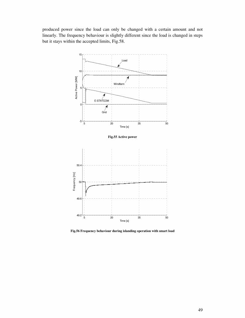
49

produced power since the load can only be changed with a certain amount and not linearly. The frequency behaviour is slightly different since the load is changed in steps but it stays within the accepted limits, Fig.58.

Fig.55 Active power

Fig.56 Frequency behaviour during islanding operation with smart load

5 20 35 50-5

0

5

10

15

Time [s]

Active

Po

we

r [M

W]

E-STATCOM

Grid

Windfarm

Load

5 20 35 5049.2

49.6

50

50.4

Time [s]

Fre

qu

en

cy [

Hz]

50

Fig.57 Active power

Fig.58 Frequency behaviour during islanding operation with smart load

5 6 8 10 12 14-5

0

5

10

15

Time [s]

Active

Po

we

r [M

W]

Load

Wind farm

E-STATCOM

Grid

6 8 10 12

49.6

49.8

50

50.1

Time [s]

Fre

qu

en

cy [

Hz]

51

Chapter 6. Conclusions and Future work

The static synchronous compensator together with an energy storage device has been described in this thesis. It was first described that it can be used for many different applications where the main application is to improve the stability of the grid by regulating the voltage. This is done by reactive power control. The idea of today is as mentioned to combine it together with some kind of energy storage device, such as a battery. The STATCOM is in this case similar to a voltage sourced converter HVDC but with a limitation in the active power. One could say that it is an HVDC only consisting of the stability enhancement properties and with limitations in the amount of power. Different control systems for the E-STATCOM have been treated in this report. The main controller inside a STATCOM is the current controller. Therefore it has been described how to derive a current controller, based on a simple network. The control is done in the dq-coordinate system because otherwise the integral part of the controller cannot be used and also resonant controller has to be used. The derived current controller was then verified in PSCAD. A step was applied in both the d and q component of the controller to see the response. According to the graphs, which can be found in the described chapter, the current controller shows really good performance. Notice that this report focuses on the active power of the E-STATCOM but the current controller is derived so that both the active and the reactive power can be controlled. To provide the reference signal to the current controller additional control systems have been derived. As mentioned the most common additional controller is the voltage controller, since the main application for a STATCOM is voltage control. This feature is briefly described in this report, the focus is instead on the frequency- and power oscillation damping controller. In this chapter the PLL and AN-PLL was described. It was stated that the AN-PLL was the best choice since it showed a better performance when connected to a weak grid. It could also provide a signal to the power oscillation damping, which the PLL cannot. The approach of deriving the frequency controller is similar to the current controller, but with another bandwidth. It has been chosen to be 10% of the bandwidth of the current controller and hence the current controller is much faster. Also how to implement the needed droop setting has been described. This controller has then been verified in PSCAD by using a grid where there is no other component controlling the frequency. The result shows that it is possible to fully control the frequency but this is however dependent on how large the load is compared to the size of the energy storage device. In the simulations it was assumed that the load was less than the size of the energy storage and therefore it was possible to control the frequency close to the rated value. The only thing preventing it from reaching rated frequency was the droop settings in the controller. It can therefore be concluded that the frequency controller works as intended and that it can be used for the intended purpose.

52

A simple controller for power oscillations damping was also created based on the proportional part of the frequency controller and it has been discussed that an E-STATCOM has the possibility to provide additional power oscillation damping in a grid, if it is connected on a proper location. It has been shown in a simple network how the oscillations behave following a transient in the grid. It was shown that the stability could be improved, and hence the power oscillation damping ability, if an E-STATCOM was connected on a proper location in the grid. The same network was then built and tested in PSCAD to compare with the mathematical calculations. Also in this case it could be seen that the stability increased when using an E-STATCOM. It should be noticed that the mathematical representation is not exactly the same as the PSCAD representation, but it can be seen from both what the frequency of the oscillation is and that the stability can be improved by using this technology. The reason for the difference between the two models is that in the mathematical model is very simple and cannot fully represent reality. It can be concluded that power oscillations can be damped within one period if active power is used and if the energy storage is large enough. This is much better than what can be done with only reactive power. This is simply because one cannot change the magnitude of the voltage too much but the amount of active power can be changed drastically, as discussed earlier. It has also been discussed that the connection point is important if the power oscillation damping ability should be optimized and the result shows that it should be as close as possible to the generator.

6.1 Falbygdens Energi AB

The trend of today is to increase the amount of wind power in the grid. As discussed before, this creates some problem since it can make the grid weak, especially if the grid is weak from the beginning. One example of such a grid is the grid in Falköping. They have a goal to increase the amount of wind power and the interim target is to install 16 MW. A part of the grid has been created in PSCAD in a collaboration work with Francisco Montes Venero. In this model different type of faults and operation modes has been tested and analyzed. It has been found out that it depends on the location of the fault if the wind turbines will survive or not. Simulations with the E-STATCOM connected to the grid has been performed and the results show that it cannot help the grid when a fault is applied somewhere in the grid. Therefore it will not be useful from a dynamical point of view. If the above is considered it should however be noticed that the model of the grid is a simplification of the real system and will therefore not behave exactly as in reality. With the first 16 MW of wind power installed the short-circuit power will still be around 10 times larger and therefore the system has to be considered to be relatively strong. This will probably change in the future when more and more wind power is installed and in that case the results could be completely different.

53

It can however be interesting to install an energy storage device for other applications. The main driving force in my opinion is to install it to store energy when the wind power is producing power and then sell this power when there is no wind. It can in this case be used for other additional applications also. These applications have been discussed in Chapter 2. One interesting case which has been tested in PSCAD is when the system enters islanding mode. It has in this case been proposed to use a “smart load” where the E-STATCOM temporarily provides power meanwhile the load is adapted to the generated wind farm power. The result shows that it is possible to do this if the power absorbed by the load exceeds the generated power from the wind farm with a maximum of 2 MW, this is because the proposed size of the energy storage is 2MW. If this size is increase the criteria changes and a larger load can be allowed. The final conclusions are therefore that the E-STATCOM is not needed from a dynamical point of view today since there is no phase angle deviation during faults. This can however be different in the future when the ratio between the short-circuit power and the installed amount of wind power is decreased. It can however be very useful today for other applications, as discussed earlier.

6.2 Future work

The focus has in this work been on the E-STATCOM for frequency control. In addition to this feature, many other applications have been purposed but they have not been further investigated. Therefore there are many opportunities to continue to investigate for future applications. One interesting field would be to continue working on the “smart load” control, which was only briefly investigated in this work. The method used here was to reduce the load linearly until it matched the produced power from the wind farm. A more detailed controller with different options could be one solution and also how to prioritize what load should be disconnected first. Another limitation in this work is the representation of the battery. This was simplified by a high pass filter to represent the discharge of a battery. A more accurate model of the battery could be investigated to give a more reliable behavior of how much energy it would be able to supply during different modes of operation. When it comes to the investigation of FEAB grid their aim is to install even more wind power and the most significant work that should be done is to increase the amount of wind power, and see how the system behaves.

54

55

APPENDIX

Three-phase to dq coordinates

The three-phase to dq transformation is a powerful tool that is useful for detection of deviations and to control different quantities. The procedure on how to perform this calculation will briefly be described in this topic. The dq coordinate system rotates with the stator frequency ω1 and therefore the steady state quantities will be represented by dc quantities. Since the steady state operation is shown in dc quantities it will be easier to detect and control deviations compared to if we directly control a constantly oscillating quantity. Due to this reason all the control systems will be created in dq coordinates by first transforming the three phase system into the αβ-system and then into the dq system. The equations to perform this transformation are shown below.

Three-phase to αβ

If we consider a symmetrical three-phase system the zero sequence component can be disregarded which means that the sum of the three phase voltages will be zero. And since they will be zero each voltage can be described by the two remaining phase voltages and hence the three-phase system can be described as a two-phase system called the αβ-system. The transformation matrix for transforming three-phase into αβ is shown below, if instead the opposite is needed the inverse of this matrix is used.

w����������x � �yzz{23 �13 �130 1√3 � 1√3~�

�� ��4����\���������

Where K is a scaling factor depending on if we want to use peak-value, RMS-value or power-invariant scaling. For peak-value scaling K=1 and for power-invariant scaling

K=o2/3

αβ to dq

To transform from αβ coordinates into dq coordinates the following matrix is used.

w����������x � w ��B5 ���B5����B5 ��B5x w����������x Where

B5 � S�5�

As for the three-phase to αβ, if the opposite is instead needed the inverse of the matrix is used.

56

57

Reference list

[1] H. P. Nee, H. Xie, and L. Ängquist, “Investigation of StatComs With

Capacitive Energy Storage for Reduction of Voltage Phase Jumps in Weak Networks,” in IEEE Transactions on power systems, vol. 24, no. 1, Feb. 2009.

[2] L. Harnefors, Control of Variable-Speed Drives. Västerås, Sweden, Sep. 2002

[3] T. Aboul-Seoud and J. Jatskevich, “Improving power quality in remote wind energy systems using battery storage,” in Electrical and Computer

Engineering, CCECE 2008, Canadian Conference. May. 2008, pp. 1743-1736.

[4] C. Du, “VSC-HVDC for Industrial Power Systems,” Ph.D thesis, Chalmers University of Technology, Göteborg, Sweden, 2007.

[5] P.Kundur, Power system stability and control. New York: McGraw-Hill 1994.

[6] J. Machowski, J. W. Bialek and J. R. Bumby, Power System Dynamics

and Stability. Chichester, England: John Wiley & Sons Ltd. 1998 [7] Nordic Grid Code.

http://www.entsoe.eu/fileadmin/user_upload/_library/publications/nordic/planning/070115_entsoe_nordic_NordicGridCode.pdf .2007

[8] M. E. Baran, S. Teleke, A. Huang, S. Bhattacharya, L. Anderson and S. Atcitty, “STATCOM with Energy Storage for Smoothing Intermittent Wind Farm Power”. Power and Energy Society General meeting –

Conversion and Delivery of Electrical Energy in the 21th Century.2008 [9] M.R.I. Sheikh, S.M. Muyeen, R. Takahashi, T. Murata and J. Tamura,

“Minimization of Fluctuations of Output Power and Terminal Voltage of Wind Generator by Using STATCOM/SMES,” in PowerTech, IEEE Bucharest, 2009

[10] M. G. Molina, P. E. Mercado and E. H.Watanabe, “Dynamic Performance of a Static Synchronous Compensator with Superconducting magnetic Energy Storage,” in Power Electronic Specialists Conference. June. 2005. pp 224-230

[11] P. M. Anderson, B. L. Agrawal and J. E. Van Ness, Subsynchronous

resonance in power systems. New York, US: IEEE Press.1990 [12] P. M. Anderson and R. G. Farmer, Series Compensation of Power

Systems, California, US: PBLSH!.1996 [13] http://www.energimyndigheten.se/sv/Energifakta/Energikallor/Vindkraft/

2010. [14] N. G. Hingorani and L. Gyugyi, Understanding FACTS: Concepts and

Technology of Flexible AC Transmission Systems, New York, US: Wiley-IEEE Press. 1999

58

[15] L. Ängquist and M. Bongiorno, “Auto-normalizing Phase-Locked Loop for grid-connected converters,” in IEEE Energy Conversion Congress and

Exposition. San Jose, US. Sept. 2009. pp 2957-2964 [16] S. G. Johansson, G. Asplund, E. Jansson and R. Rudervall, “Power system

stability benefits with vsc dc-transmission systems,” CIGRÉ conference in Paris, France, 2004

[17] M. Bongiorno, J. Svensson and A.Sannino, “Effect of Sampling Frequency and Harmonics on Delay-Based Phase-Sequence Estimation Method,” in IEEE Transactions on power delivery, July 2008. Pp 1664-1672

[18] J. Perez-Ramirez, V. Cardenas, H. Miranda and G. Espinosa-Perez, ”Generalized DC voltage regulation strategy for n:1 relation cascade H-bridge converter based STATCOM,” in IEEE Energy conversion congress

and exposition, San Jose, US. Sept. 2009. Pp 2985-2990 [19] R. Mohan Mathur and R. K. Varma, Thyristor-based FACTS controllers

for electrical transmission systems, New York, US. John Wiley & Sons Ltd. 2002