use of gis to find optimum locations for anaerobic

The University of Maine The University of Maine

DigitalCommons@UMaine DigitalCommons@UMaine

Electronic Theses and Dissertations Fogler Library

Fall 12-20-2020

Use of GIS to Find Optimum Locations for Anaerobic Digestion or Use of GIS to Find Optimum Locations for Anaerobic Digestion or

Composting Facilities in Maine Composting Facilities in Maine

Usha Humagain University of Maine, [email protected]

Follow this and additional works at: https://digitalcommons.library.umaine.edu/etd

Part of the Civil and Environmental Engineering Commons, and the Geographic Information Sciences

Commons

Recommended Citation Recommended Citation Humagain, Usha, "Use of GIS to Find Optimum Locations for Anaerobic Digestion or Composting Facilities in Maine" (2020). Electronic Theses and Dissertations. 3366. https://digitalcommons.library.umaine.edu/etd/3366

This Open-Access Thesis is brought to you for free and open access by DigitalCommons@UMaine. It has been accepted for inclusion in Electronic Theses and Dissertations by an authorized administrator of DigitalCommons@UMaine. For more information, please contact [email protected].

https://digitalcommons.library.umaine.edu/

https://digitalcommons.library.umaine.edu/etd

https://digitalcommons.library.umaine.edu/fogler

https://digitalcommons.library.umaine.edu/etd?utm_source=digitalcommons.library.umaine.edu%2Fetd%2F3366&utm_medium=PDF&utm_campaign=PDFCoverPages

http://network.bepress.com/hgg/discipline/251?utm_source=digitalcommons.library.umaine.edu%2Fetd%2F3366&utm_medium=PDF&utm_campaign=PDFCoverPages



https://digitalcommons.library.umaine.edu/etd/3366?utm_source=digitalcommons.library.umaine.edu%2Fetd%2F3366&utm_medium=PDF&utm_campaign=PDFCoverPages

mailto:[email protected]

USE OF GIS TO FIND OPTIMUM LOCATIONS FOR ANAEROBIC

DIGESTION OR COMPOSTING FACILITIES IN MAINE

By

Usha Humagain

B.E. Tribhuvan University, 2016

A THESIS

Submitted in Partial Fulfillment of the

Requirements for the Degree of

Master of Science

(in Civil Engineering)

The Graduate School

The University of Maine

December 2020

Advisory Committee:

Dr. Jean D. MacRae, Associate Professor of Civil and Environmental

Engineering, Advisor

Dr. Kate Beard, Professor in School of Computing and Information Science

Travis Blackmer, Lecturer and Undergraduate Coordinator in School of

Economics

USE OF GIS TO FIND OPTIMUM LOCATIONS FOR ANAEROBIC

DIGESTION OR COMPOSTING FACILITIES IN MAINE

By Usha Humagain

Thesis Advisor: Dr. Jean D. Macrae

An Abstract of the Thesis Presented

in Partial Fulfillment of the Requirements for the

Degree of Master of Science

(in Civil Engineering)

December 2020

As per US EPA, in 2017, 41 million tons of food waste was generated, but only

6.3% was diverted from landfills (US EPA, 2020). When landfilled or incinerated,

organic waste (food waste, sludge, manure, agricultural waste) causes environmental

pollution through greenhouse gas emissions, land, water, and air pollution. In contrast, if

we compost or digest organic waste, we can generate soil additives and a mixture of

methane and carbon dioxide gas to produce electricity or energy. Both digestion and

composting reduce greenhouse gas emissions, improve the land through additives, and

boost the economy. Many countries are adopting anaerobic digestion and composting to

handle organic waste. There are currently 250 anaerobic digesters in the US (Pennington,

2018). There are 1200 wastewater recovery facilities in the US with anaerobic digestion,

and approximately 20% of them co-digest sludge with other organic materials

(Pennington, 2019).

Meanwhile, the process of anaerobic digestion is chemically and biologically

complex. In 2018 alone, as per EPA, eleven anaerobic digesting facilities were shut down

(Pennington, 2019). There were various underlying factors such as; lack of feedstock,

economic infeasibility, system shock, hampering the sensitive areas like wetlands through

leaching from the storage areas. Thus, while starting a facility, there are many factors to

consider for its long-run success. One of the most crucial factors to consider is the site

location. Social acceptance, economic viability, job opportunities, and environmental

disturbance are all site-dependent. Hence it is critical to optimize the choice.

This study used ArcGIS Pro 2.6 to find the optimum location for organic waste

management facilities in Maine. There are three anaerobic digesters in Maine, of which

one is currently closed, and approximately 92 composting facilities handle a large amount

of yard trimmings and some food waste. Most of the composting facilities are small scale

with 4.3% composting food waste and 4.3% composting sewage sludge. In this study,

data on food waste, manure, and sludge were gathered from Maine DEP, EPA, US Farms

Data, and published reports to estimate the approximate amount of organic waste. A

capture rate of 20% was used for food waste to estimate the amount of food waste

collected. For the analysis, four scenarios: (1) the largest anaerobic digester (Fiberight)

does not resume, or (2) resumes its work, and (3) co-digesting waste with or (4) without

sludge were taken into consideration. To be more area-specific, the analysis was done for

the Maine Department of Transportation (DOT) regions: Eastern, Northern, Southern,

Mid-Coast, and Western Regions. Eight criteria- food waste availability, sludge

availability, transportation cost, distance from residential areas, slope, land cover,

distance from airports, and environmentally sensitive areas like conserved lands and

wetlands were used to find the optimum locations. Analytical Hierarchy Process

determined the criteria weights before assigning them in the suitability modeler of

ArcGIS Pro to find the optimum locations. By transforming these criteria, the five best

locations in Maine and three possible optimum locations in each region for each scenario

were identified. Opportunities for the upgrading of existing farms with excess manure,

transfer stations, composting facilities, and WRRFs were identified.

The facilities that coincide in all the scenarios are the optimum facilities that work

in all scenarios. Hence feasibility study can be started on those facilities. In the Northern

region, Caribou WWTF and Pinelands Farms Natural Meats Inc. coincide in all

scenarios, making them the best existing facilities that could be upgraded in the future.

Similarly, in the Eastern region, the transfer station of the Town of Lincoln, and the

Dover Foxcroft WRRF coincide in all scenarios, making them the best existing facilities

that could be upgraded in the Eastern region. Four farms and the transfer station of the

town of Clinton coincide in all scenarios in Mid-Coast. Out of these four farms, Stedy

Rise farms and Caverly Hills LLC are 330 acres and 840 acres and generate excess

manure of 4096 tons /year and 4175 tons/year. These farms could be good locations for a

new facility using food waste. In the Southern region, no single facility was identified in

all the scenarios, but Sanford WRRF and a few farms could be chosen for feasibility

analysis. In the Western region, six farms and the transfer station of the town of Turner

coincide in all the scenarios. Feasibility analysis can be done in these facilities to

determine which can be upgraded as a new waste management facility utilizing food

waste.

ii

ACKNOWLEDGMENTS

I want to thank my advisory committee for the regular feedback on my project

and for working with me on this. My advisor, Dr. Jean D. MacRae, has continuously

supported me and helped me with the new waste-related information. She has always

pushed me forward to learning new things and showing my works to the community. I

am thankful to her. Being an international student and having English as a second

language was pretty tough for me to gain confidence. These two and half years in the

University has made me more confident to express myself. I am glad I chose this

University for my master's degree. My second family: the Nepalese students of Maine,

has never made me feel alone and far away from family and friends. Finally, I want to be

thankful to my family and friends back home, who always have believed in me.

iii

TABLE OF CONTENTS

ACKNOWLEDGMENTS ........................................................................................ II

LIST OF TABLES ................................................................................................. VII

LIST OF FIGURES ................................................................................................ IX

CHAPTER 1 USE OF GIS TO FIND OPTIMUM LOCATION FOR

ANAEROBIC DIGESTER OR COMPOSTING FACILITIES ................................ 1

1.1 INTRODUCTION .............................................................................................................. 1

1.1.1 ANAEROBIC DIGESTION ........................................................................................... 1

1.1.2 COMPOSTING............................................................................................................... 4

1.1.3 WASTE MANAGEMENT IN THE UNITED STATES ............................................... 5

1.1.4 WASTE MANAGEMENT IN MAINE.......................................................................... 7

1.1.5 THE RATIONALE OF THE STUDY ............................................................................ 9

1.1.6 OBJECTIVES OF THE STUDY .................................................................................. 10

1.2 METHODOLOGY ........................................................................................................... 10

1.2.1 ARCGIS PRO ANALYSIS .......................................................................................... 10

1.2.2 WASTE MANAGEMENT SCENARIOS .................................................................... 11

1.2.3 DIVIDING MAINE INTO WASTE MANAGEMENT AREAS ................................. 12

1.2.4 DATA COLLECTION AND ASSUMPTIONS ........................................................... 14

1.2.5 SUITABILITY MODELER ......................................................................................... 27

1.2.6 ANALYTICAL HIERARCHY PROCESS (AHP) ...................................................... 28

iv

1.2.7 USE OF THE MODELER AND THE TRANSFORMATION TO THE CRITERIA . 34

1.3 DATA ANALYSIS AND INTERPRETATION .............................................................. 39

1.3.1 ORGANIC WASTE IN MAINE .................................................................................. 39

1.3.2 OPTIMUM LOCATIONS FOR ADDITIONAL FACILITIES ................................... 44

1.3.3 UPGRADING OF FACILITIES................................................................................... 54

1.4 CONCLUSIONS............................................................................................................... 64

1.5 THE SENSITIVITY OF THE METHODOLOGY .......................................................... 65

1.6 FUTURE AREAS FOR RESEARCH .............................................................................. 67

CHAPTER 2 LAB TECHNIQUE TO OBSERVE SALT AND AMMONIA

TOXICITY ............................................................................................................68

2.1 INTRODUCTION ............................................................................................................ 68

2.2 METHODS AND MATERIALS ...................................................................................... 69

2.2.1 SEED DIGESTER ........................................................................................................ 69

2.2.2 COLLECTION AND PROCESSING OF THE SUBSTRATE ................................... 71

2.2.3 SODIUM TOXICITY EXPERIMENT......................................................................... 72

2.2.4 AMMONIUM TOXICITY ........................................................................................... 73

2.2.5 CHEMISTRY METHODS ........................................................................................... 75

2.2.6 pH .................................................................................................................................. 75

2.2.7 VOLATILE SOLIDS .................................................................................................... 75

2.2.8 ALKALINITY .............................................................................................................. 76

v

2.2.9 VOLATILE FATTY ACIDS (VFAS) .......................................................................... 77

2.2.10 GAS COMPOSITION .............................................................................................. 77

2.2.11 CONDUCTIVITY .................................................................................................... 78

2.2.12 AMMONIUM ........................................................................................................... 79

2.3 RESULTS AND DISCUSSION ....................................................................................... 80

2.3.1 PERFORMANCE OF THE SEED DIGESTER ........................................................... 80

2.3.2 EFFECT OF SODIUM ION IN ANAEROBIC DIGESTERS ..................................... 81

2.3.3 EFFECT OF AMMONIUM ION IN ANAEROBIC DIGESTERS ............................. 83

2.3.4 VARIABILITY OF THE RESULTS............................................................................ 85

2.4 CONCLUSIONS............................................................................................................... 85

BIBLIOGRAPHY ....................................................................................................87

CHAPTER 3 APPENDICES ...................................................................................92

3.1 APPENDIX A: SUITABILITY MAPS ............................................................................ 92

3.1.1 MAINE ......................................................................................................................... 92

3.1.2 NORTHERN REGION ................................................................................................. 93

3.1.3 EASTERN REGION .................................................................................................... 94

3.1.4 MID-COAST REGION ................................................................................................ 95

3.1.5 SOUTHERN REGION ................................................................................................. 96

3.1.6 WESTERN REGION.................................................................................................... 97

3.2 APPENDIX B: CRITERIA WEIGHTS BY AHP ............................................................ 98

vi

3.2.1 ECONOMIC FACTORS .............................................................................................. 98

3.2.2 TECHNICAL FACTORS ........................................................................................... 100

3.2.3 ENVIRONMENTAL FACTORS ............................................................................... 101

3.3 APPENDIX C: CALIBRATION CHARTS ................................................................... 103

3.4 APPENDIX D: SODIUM EXPERIMENT ..................................................................... 104

3.5 APPENDIX D: AMMONIA EXPERIMENT ................................................................ 105

CHAPTER 4 BIOGRAPHY OF THE AUTHOR ..................................................107

vii

LIST OF TABLES

Table 1-1: Details of Maine DOT Regions ........................................................................13

Table 1-2: Typical national values for municipal wastewater ...........................................17

Table 1-3: Summary of data and their uses .......................................................................27

Table 1-4: AHP numbers ...................................................................................................30

Table 1-5: Criteria for AHP and Suitability modeler.........................................................32

Table 1-6: Criteria weights for sludge exclusion method ..................................................33

Table 1-7: Criteria weights for sludge inclusion method...................................................34

Table 1-8: Summary of the optimum locations in each region ..........................................53

Table 1-9: Facilities that can be upgraded in Maine DOT regions in different

scenario .............................................................................................................60

Table 1-10: Comparison of optimum locations determined using different global

weighting schemes ............................................................................................66

Table 2-1: Detail of the batches for salt toxicity experiment .............................................73

Table 2-2: Details of the batches for ammonium toxicity .................................................74

Table 3-1: Assigned AHP numbers to economic factors in sludge exclusion ...................98

Table 3-2: Normalized matrix for sludge exclusion ..........................................................98

Table 3-3: Consistency Index for sludge exclusion ...........................................................98

Table 3-4: AHP numbers assigned to sludge inclusion .....................................................99

Table 3-5: Normalized matrix for sludge exclusion ..........................................................99

viii

Table 3-6: Consistency Index for sludge exclusion ...........................................................99

Table 3-7: AHP numbers assigned to technical factors ...................................................100

Table 3-8: Normalized matrix for technical factors .........................................................100

Table 3-9: Consistency Index for technical factors .........................................................100

Table 3-10: AHP numbers assigned to environmental factors ........................................101

Table 3-11: Normalized matrix for environmental factors ..............................................101

Table 3-12: Consistency Index for environmental factors ...............................................101

Table 3-13: Criteria weights for sludge exclusion (Case 1) ............................................102

Table 3-14: Criteria Weights for the sludge inclusion (Case 1) ......................................102

ix

LIST OF FIGURES

Figure 1-1: Anaerobic digestion process (Leal, 2020) .........................................................2

Figure 1-2: Food Recovery Hierarchy by EPA (EPA, 2019) ..............................................6

Figure 1-3: Scenario for waste management in Maine ......................................................12

Figure 1-4: Five regions used for site optimization ...........................................................13

Figure 1-5: Cluster of Livestock Farms in Maine. .............................................................15

Figure 1-6: Clusters of municipal wastewater recovery facilities in Maine ......................19

Figure 1-7: Location of composting facilities as per the EPA data (Excess Food

Opportunities Map, n.d.). .................................................................................22

Figure 1-8: Transfer stations in Maine...............................................................................23

Figure 1-9: Maine conserved lands. ...................................................................................24

Figure 1-10: Wetlands of Maine ........................................................................................25

Figure 1-11: Sludge generation in Maine by wastewater recovery facilities. ....................40

Figure 1-12: Food waste generation in Maine by towns and township polygons. ............41

Figure 1-13: Heatmap to show excess manure generation in Maine. ................................42

Figure 1-14: Towns served by existing anaerobic digesters. .............................................43

Figure 1-15: Optimum locations in Maine if Fiberight is operational and sludge is

treated with food waste .....................................................................................45

Figure 1-16: Optimum locations in Maine DOT regions if Fiberight is operational

and sludge is treated with food waste ...............................................................46

x

Figure 1-17: Optimum locations in Maine if Fiberight is operational and sludge is

excluded from treatment ...................................................................................47

Figure 1-18: Optimum locations in Maine DOT region if Fiberight is operational

and the sludge is excluded from treatment ........................................................48

Figure 1-19: Optimum Locations in Maine if Fiberight is not operational and

sludge is treated with food waste ......................................................................49

Figure 1-20: Optimum locations in Maine DOT regions if the Fiberight is not

operational and the sludge is treated with food waste.......................................50

Figure 1-21: Optimum Locations in Maine if Fiberight is not operational and

sludge is excluded .............................................................................................51

Figure 1-22: Optimum Locations in Maine DOT regions when Fiberight is not

operational, and sludge is excluded from treatment..........................................52

Figure 1-23: Upgrading of existing facilities in Maine DOT regions if Fiberight is

operational and sludge is treated with food waste ............................................55

Figure 1-24: Upgrading of existing facilities in Maine DOT regions if Fiberight is

operational and sludge is excluded from treatment...........................................56

Figure 1-25: Upgrading of existing facilities in the Maine DOT regions if

Fiberight is not operational and sludge is treated with food waste ...................58

Figure 1-26: Upgrading of facilities in Maine DOT regions if Fiberight is not

operational and sludge is excluded from treatment...........................................59

Figure 2-1: Mechanism of the new digester. .....................................................................71

xi

Figure 2-2: Monitoring the pH, sodium ion concentration, the acid accumulation

in the system. .....................................................................................................80

Figure 2-3: VSS destruction at different sodium concentration ........................................82

Figure 2-4: Methane yield at different concentration of sodium ion .................................82

Figure 2-5: VS destruction at different ammonium nitrogen concentrations in the

sample ...............................................................................................................84

Figure 2-6: Methane yield at different concentrations of ammonium-nitrogen ................84

Figure 2-7: Ammonium concentration at the beginning and the end of the

experiment. ........................................................................................................85

Figure 3-1: Suitability map of Maine.................................................................................92

Figure 3-2: Suitability map of Northern region. ................................................................93

Figure 3-3 Suitability map of Eastern region .....................................................................94

Figure 3-4: Suitability map of Mid-Coast region ..............................................................95

Figure 3-5: Suitability map of Southern region .................................................................96

Figure 3-6: Suitability map of the Western region ............................................................97

Figure 3-7: Calibration chart for conductivity .................................................................103

Figure 3-8: Calibration chart for ammonium concentration ............................................103

Figure 3-9: Experimental pictures for salt toxicity test. ..................................................105

Figure 3-10: The top left picture represents the pre-autoclaved labeled serum

bottles just before the experiment. ..................................................................106

xii

Figure 3-11: The seed digester. ........................................................................................106

1

CHAPTER 1

USE OF GIS TO FIND OPTIMUM LOCATION FOR ANAEROBIC DIGESTER OR

COMPOSTING FACILITIES

1.1 INTRODUCTION

Globally the Food and Agriculture Organization of the United Nations (FAO) has

estimated that one-third of food produced for human consumption is lost or wasted,

equivalent to about 1.3 billion tonnes per year, with the highest proportion contributed by

household waste (IEA Bioenergy, 2018). In the U.S. in 2017 alone, EPA estimates that

almost 41 million tons of food waste was generated, with only 6.3% diverted from

landfills and incinerators (US EPA, 2020). Piles of food waste and other organic waste

contributed from municipal solid waste, wastewater, and food processing waste fill up the

landfills and impact the environment with greenhouse gas emissions, air, water, and land

pollution (IEA Bioenergy, 2018). We need a shift towards a renewable and sustainable

system to circularize the food system. There are various measures to reduce organic

wastes like source reduction, feeding excess food to people and animals, composting,

waste-to-energy technologies like anaerobic digestion, and incineration; however, this

study focuses only on anaerobic digestion and composting.

1.1.1 ANAEROBIC DIGESTION

Carbon dioxide fixed into organic matter by photosynthesis is regenerated upon the

decomposition of organic matter by O2, requiring (aerobic) organisms in aerated habitats

(Wall et al., 2008). Under anaerobic conditions, a complex mixture of symbiotic

microorganisms can also decompose organic materials into a mixture of gas called

2

biogas, consisting of methane, carbon dioxide, hydrogen sulfide, and moisture; plus,

nutrients and additional cell matter (Wall et al., 2008). This process is commonly known

as anaerobic digestion. David Fulford describes anaerobic digestion as the process that

uses naturally occurring microorganisms to break down organic materials-food waste,

wastewater sludge, agricultural waste, or manure - into methane and carbon dioxide in

the absence of oxygen (Fulford, 2015).

Figure 1-1: Anaerobic digestion process (Leal, 2020)

Fermentative

Bacteria Fermentative

Bacteria

Intermediary Products

Propionate, Buy rate

(Short Chain Volatile Organic Acids)

Fermentative

Bacteria

Complex Polymers

(Proteins, Carbohydrates, Lipid)

Monomers

(Sugars, amino acids, peptides, fatty acids)

Fermentative Bacteria

Acetogens (H2 Producing)

H2+CO2 Acetate

CO2 reducing

methanogens

Acetoclastic

methanogens

CH4+CO2

Acetogenesis

Hydrolysis

Acidogenesis

Methanogenesis

3

Anaerobic digestion completes in four biological processes: hydrolysis, acidogenesis,

acetogenesis, and methanogenesis.

In the hydrolysis process, microbes break down the chemical bonds by incorporating a

water molecule. Complex molecules like carbohydrates, proteins, lipids, and cellulose are

broken down into smaller molecules like sugars, amino acids by hydrolytic bacteria with

extracellular enzymes like amylase for carbohydrates, cellulase for cellulose, lipase for

lipids, and protease for proteins (Kim et al., 2012). This step occurs very slowly; thus,

this step can be a rate-limiting step in anaerobic digestion (Kim et al., 2012). The

hydrolysis rate depends on the size and type of organic materials, pH, temperature, salt

content, metals, and enzymes (Ali Shah et al., 2014). The compounds formed in the

hydrolysis stage ferment into alcohols like ethanol and acids like propionic, acetic,

valeric, and butyric acids in acidogenesis (Mir et al., 2016). In acetogenesis, the

acidogenesis phase products convert to acetate, carbon dioxide, and hydrogen (Mir et al.,

2016). Methanogenesis is the final step in the anaerobic digestion of organic matter,

where methanogenic archaea are responsible for utilizing acetate, hydrogen, and carbon

dioxide to produce methane. There are three types of methanogens: acetoclastic (acetate

to methane and carbon dioxide), hydrogenotrophic (hydrogen and carbon dioxide to

methane), and methylotrophic (methyl compounds like methanol, methylamines, methyl

sulfides to methane) methanogens (Amani et al., 2010). Generally, acetoclastic

methanogens make 3/4th of methane production, contributing to the largest amount (Wall

et al., 2008). Among all the processes, acidogenesis is generally faster and can lead to the

accumulation of volatile fatty acids in the system, making the system acidic and inhibit

methanogens responsible for methane production (Wisconsin Department of Natural

4

Resources, 1992). However, in a well operating system, methanogens keep up, and the

pH remains stable. (Wisconsin Department of Natural Resources, 1992).

1.1.2 COMPOSTING

Composting, an aerobic microbial transformation, and stabilization of organic matter is

an exergonic process that releases energy, about 50– 60 % of this energy is utilized by

microorganisms to synthesize ATP; the remainder loses as heat (Stentiford & de Bertoldi,

2010). In practice, there are four main activities required for efficient composting,

namely: shredding, to reduce particle size and increase the surface area to volume ratio;

mixing different feedstocks to improve homogeneity and adjust the carbon to nitrogen (C:

N) ratio; adding water where mainly dry materials are received; and removing

contaminants (Swan et al., 2002). A typical composting process completes in four phases.

1. Mesophilic Phase: A diverse population of mesophilic bacteria and fungi

proliferates and degrade readily available organic matter, thereby increasing the

temperature to about 45 C.

2. Thermophilic Phase: Temperature increases to 55-65 C and this heat eliminates

pathogenic and helminths eggs.

3. Cooling Phase: Temperature decreases and remains at about 25-30 C, also

known as the stabilization or curing phase.

4. Humification Phase: The humic acid content and cation exchange capacity of

compost increases.

(Stentiford & de Bertoldi, 2010; Williams et al., 2002).

5

Anaerobic digestion technology has two significant advantages over composting: firstly,

it is cost-effective for use at large scale and with “strong” wastes because it does not

require aeration and produces a small amount of excess sludge. Secondly, it recovers

some of the energy content of the organic matter as gaseous methane (Narihiro &

Sekiguchi, 2007). On the other hand, composting facilities are simpler to operate, easier

to expand, require less capital investment, can accept variable input materials (by type

and amount) and produce a more stable product (Mohee & Mudhoo, 2012).

1.1.3 WASTE MANAGEMENT IN THE UNITED STATES

As per the EPA's resource recovery hierarchy (EPA, 2019) shown in

Figure 1-2, the least preferred waste management method is landfilling and incineration,

followed by composting and anaerobic digestion, industrial uses, feed people and animals

and source reduction. There are programs like EPA's Food Too Good To Waste

Program, which uses consumer education and awareness through its pilot projects to

recover food. Consumers are also provided with shopping bags, measurement tools, and

tips for food storage and meal planning as a measure to reduce food waste (Hobson,

2006).

6

Figure 1-2: Food Recovery Hierarchy by EPA (EPA, 2019)

The total municipal solid waste (MSW) generation in 2017 was 267.8 million tons or 4.5

pounds per person per day. From this MSW, 27 million tons were composted, of which

2.6 million tons was food waste, and the remainder was yard trimmings (OLEM US EPA,

n.d.). More than 139 million tons of MSW, out of which 22% was food, were landfilled

(OLEM US EPA, n.d.). AgSTAR estimates that biogas recovery is technically feasible at

over 8000 large dairy and hog operations that can potentially generate nearly 16 million

MWh of energy per year and displace about 2010 MWs of fossil fuel-fired generation

(OAR US EPA, n.d.). Meanwhile, as per EPA's AgSTAR program, approximately 250

anaerobic digesters are operating on livestock farms in the USA (Pennington, 2018).

Forty-three of these anaerobic digesters co-digest food waste with manure (Pennington,

2018). There are 58 stand-alone anaerobic digesters that are built to digest food waste

(Pennington, 2018). The Water Environment Federation and American Biogas Council

database identify about 1200 Wastewater Resource Recovery Facilities (WRRFs) in the

7

U.S. that use anaerobic digestion to manage wastewater sludge. Of these, roughly 20%

co-digest food waste received from other sources (Pennington, 2019).

1.1.4 WASTE MANAGEMENT IN MAINE

In Maine, unit-based pricing for waste disposal "pay as you throw" (PAYT) is in place in

more than 160 communities (Isenhour et al., 2016). There are currently three anaerobic

digesters digesting sludge and food processing waste, manure and FW, soluble organics

from MSW and composting facilities that compost FW with other kinds of organic waste.

There are transfer stations that collect and transfer the municipal waste to the

corresponding site.

1.1.4.1 Anaerobic digesters in Maine

1.1.4.1.1 Exeter Agri-Energy:

Exeter Agri-Energy is a renewable energy company using manure from the Stonyvale

farm of Exeter, Maine, and organic waste from Scarborough and different communities

around Portland, Hannaford grocery stores around Maine and Walmart (ecomaine, 2017).

Agri-Cycle, a food waste collection service, delivers industrial loads of food waste from

area supermarkets, restaurants, and food processors in Greater Portland to Exeter Agri-

Energy (ecomaine, 2017). Stonyvale farm collects manure from 1000 milking cows. It

mixes with the organic waste collected from different areas to produce electricity and

heat, organic fertilizer, organic soil additives, healthy and comfortable animal bedding.

The system heats the mixture to just over 100 degrees Fahrenheit and agitates it

intermittently over a 15-25 days retention period. A 1500 horsepower engine burns the

biogas produced, powering the generator that produces enough heat every day to replace

700 gallons of heating oil on average and 22000 KW hours of electricity. On an annual

8

basis, this energy is enough to heat 300 New England homes and enough to power as

many as 800 households.

(How It Works | EAE – Exeter Agri-Energy, n.d.)

1.1.4.1.2 Fiberight Inc:

Fiberight Inc., a next-generation waste processing facility in Hampden, Maine, processes

municipal solid waste for the Municipal Review Committee (MRC) member

communities (Fiberight, 2018). The MRC is a group of 115 Maine cities and towns

joined together as a nonprofit organization to manage their municipal solid waste (MSW)

(MRC Inc., 2018b). All the members have contracted to process their MSW in this

facility (MRC Members, n.d.). MRC members are collectively anticipated to deliver

100,000 tons of MSW annually (MRC Inc., 2018b). After delivery of the municipal solid

waste to Fiberight, it is sorted, removing the inert materials, bulky items, and recyclables.

The rest of the waste is pulped, and the remaining plastics are separated from pulped

organic materials. The organic pulp is washed to remove contaminants, and dirty water is

sent to an anaerobic digester. Clean pulp is used to make new paper products, biomass

fuel, or converted to sugars. Anaerobic digesters process the sugars from the clean pulp.

(MRC Inc., 2018a)

Meanwhile, as per Bangor daily news, Fiberight Inc. is temporarily closed as of June

2020 (Bangor Daily News, 2020) without fully reaching full operation since the planned

April 2018 start. This closure has forced 115 communities to divert their municipal waste

to landfills (Bangor Daily News, 2020).

9

1.1.4.1.3 Lewiston Auburn Water Pollution Control Authority

(LAWPCA)

LAWPCA provides wastewater treatment services to Lewiston and Auburn. Starting its

operation in 1974, the plant was one of the first secondary wastewater treatment plants in

the state. The plant has digested wastewater sludge since 2013 and additionally accepts

grease and food processing waste to generate additional biogas and electricity. The

capacity of the digester is 45000 gallons of waste/day.

(About Us – LAWPCA, n.d.)

1.1.4.2 Composting Facilities

Many companies compost waste and provide subscription-based service with the regular

pickup of organic materials. There are a mix of household, commercial, and industrial

focused companies. These companies include Garbage to Garden, We Compost It!, Mr.

Fox Composting, Project Earth (NRCM, 2016a), and Scrapdog Community Composting.

These facilities serve greater Portland, Lincoln county, southern Maine (NRCM, 2016b),

and the Mid-Coast region.

1.1.5 THE RATIONALE OF THE STUDY

Additional waste management capacity can be obtained by upgrading existing facilities

or by constructing new one. However, if we want to build or upgrade any facility, we

need to understand the different parameters like availability of feedstock, transportation

cost, geographic location, competitors and market availability for the products. Selecting

suitable areas among several possible alternatives, is the most crucial step for pollution

control and minimizing environmental hazards (Nazari et al., 2012). Hence locating a

facility is an essential aspect of the successful operation of a waste management facility.

10

There are several methods for selecting a site while considering multiple attributes, but

we chose the Geographic Information System (GIS) for better visual representation and

analysis.

1.1.6 OBJECTIVES OF THE STUDY

With the 712 livestock farms, 155 municipal WRRFs, and 318 pounds of FW generation

per person per year, Maine generates a large amount of organic waste. There are only

three anaerobic digestion facilities, with one closed at the moment, which leaves a large

amount of waste to be managed. The state of Maine has a goal, started in 1994, of

diverting 50% of total waste generated away from the landfill by January 1, 2021, and

has yet to meet the goal (Public Law Chapter 461, n.d.). The broader availability of

organics diversion would help meet this goal while removing a fraction of waste that

produces a management problem in landfills and incineration. This study aimed to find

the optimum locations to divert more food waste and ensure that all parts of the state have

viable FW management options while considering transportation, slope, land cover, FW

and sludge availability, environmentally sensitive areas, and distance to airports and

residential areas. ArcGIS pro 2.4 and 2.6 versions were used for the analysis.

1.2 METHODOLOGY

1.2.1 ARCGIS PRO ANALYSIS

ArcGIS Pro is the latest professional desktop GIS application from Esri that can explore,

visualize, analyze data; create 2D maps and 3D scenes, and share users’ work

with ArcGIS Online or ArcGIS Enterprise portal (About ArcGIS Pro—ArcGIS Pro |

Documentation, n.d.). This study used ArcGIS Pro 2.4 for data representation in the map,

finding the approximate amount of waste generated and the amount of waste that needs

11

management. ArcGIS 2.6, released in July 2020, contained the suitability modeler in

which one could use different criteria of different weights to find a suitable location,

precisely what this study aimed for. Thus, for finding appropriate locations in each

designated polygonal area, ArcGIS pro 2.6.1 was used. The coordinate system used for

the analysis was WGS 1984 UTM zone 19 N. Tools like the clip, intersect, spatial join,

join, geocode, feature to raster, and many others were used for the analysis.

1.2.2 WASTE MANAGEMENT SCENARIOS

The biosolids characteristics that affect their suitability for land application and beneficial

reuse include organic content, nutrients, pathogens, metals, and toxic organics

concentrations (Metcalf & Eddy, 2003). Some chemicals like highly halogenated

compounds and heavy metals are not readily amenable to biological degradation and

stabilization, and microbial degradation may lead to more toxic or mobile substances than

the parent compounds (Mohee & Mudhoo, 2012). There is growing concern about PFAS

(Per- and Poly-FluoroAlkyl Substances) as they are persistent in the environment and the

human body, and they accumulate (US EPA, 2018). PFAS are found in a wide range of

consumer products. Some of these compounds cause low infant birth weights, effects on

the immune system, and cancer (US EPA, 2018). Thus, there are concerns that digestion

or composting of biosolids with other organic wastes for application to agricultural soils

may amplify these bioaccumulative chemicals in the food system (National Sewage

Sludge, 2020).

Given the uncertainty around the reopening of Fiberight, two scenarios – Fiberight remaining

out-of-operation and resuming operations were considered to observe the impact on the optimum

location. Two other conditions, allowing for, or excluding wastewater treatment plant sludge,

12

were also added creating the four scenarios shown in Figure 1-3.Scenario for waste management

in Maine

Figure 1-3: Scenario for waste management in Maine

1.2.3 DIVIDING MAINE INTO WASTE MANAGEMENT AREAS

The Department of Transportation (DOT) of Maine has divided Maine into five regions-

mid-coast, southern, eastern, northern and western. These regions are presented in Figure

1-4 with their population. The optimum locations were determined for these regions in

each scenario. As per Table 1-1, the Southern region has the highest population density of

191 people/square mile, whereas the Northern region has the lowest at 6 people/mi2.

Organic Waste

Fiberright Operational

Sludge excluded from

treatment

Sludge included

Fiberright Not Operational

Sludge excluded from

treatment

Sludge Included

13

Figure 1-4: Five regions used for site optimization

Table 1-1: Details of Maine DOT Regions

Region 2020 Total

Population

Area (sq.

miles)

Population per

square miles

Towns and

Township

polygons

Eastern 249,243 7,884.022 32 3109

Mid-Coast 271,820 3,835.56 71 2902

Northern 83,769 12,896.28 6 348

Southern 651,650 3,408.6 191 1585

Western 121,685 7,191.54 17 473

14

1.2.4 DATA COLLECTION AND ASSUMPTIONS

1.2.4.1 Farms of Maine

US Farm Data is a part of the U.S. crop production industry that keeps a database of

farmers and ranchers in the US, crop type, livestock type, and operation size (Dun &

Bradstreet, 2020). A dataset of livestock farms from US Farm Data depicting the number

and type of livestock, farm area, and contact information of Maine's farms was bought

(US Farm Data, 2020). Based on that data, there were 772 farms in Maine with livestock-

cattle, dairy, pigs, Hogs, Sheep, Goats. Four hundred eighty-two farms of this dataset had

their area provided in acres.

1.2.4.1.1 Assumptions to be made on the manure production by each

livestock:

Manure production differs based on animal weight and milk production: a 1000 pounds

cow produces 82-97 pounds/day manure (Fischer, 1998; USDA & Natural Resource

Conservation Service, 1995). As per USDA, under the best conditions, only 90-95%

manure can be collected (USDA & Natural Resource Conservation Service, 1995). A

manure production rate of 100 pounds/day and 90% collection rate was assumed since

the actual weight and breed of cattle, and milk production rate were unknown.

1.2.4.1.2 Excess Manure generation from farms

Hay is an essential source of food for livestock. Alfalfa is the primary hay crop grown in

the US since it produces more than 119 million tons of hay every year (EPA, 2015). This

study estimates that each livestock farm grows hay (Alfalfa) as feedstock. The manure

application rate for Alfalfa hay's growth is seven tons-manure/acre (Undersander et al.,

2011). Any farm with more than 7 tons of manure/acre had excess manure. These farms

15

were selected for further analysis. The data obtained from US Farm Data was uploaded

and geocoded, and the geocoding resulted in only 765 farms. Figure 1-5 shows the

location of farms with excess manure in Maine. It shows that most of the farms are

concentrated between Bangor, Augusta, and Portland.

Figure 1-5: Cluster of Livestock Farms in Maine.

1.2.4.2 Wastewater Resource Recovery Facilities

EPA keeps a record of wastewater recovery facilities in the United States. This GIS

dataset contains data collected in January 2020 on wastewater recovery facilities, based

on EPA's Facility Registry Service (FRS), EPA's Integrated Compliance Information

16

System (ICIS) (EPA Facility Registry Service, n.d.). The primary facility and location

information of wastewater treatment plants was compiled from EPA Facility Registry

Service (FRS), and attribute data was collected from ICIS (EPA Facility Registry

Service, n.d.). As the study focused only on municipal wastewater treatment plants,

industrial, groundwater, and fish treatment plants were filtered from the data. After

cleaning the data, there were 155 municipal wastewater treatment plants in Maine.

Department of Environmental Protection has a dataset on WRRFs with its licensed flow.

The data was downloaded in shapefile from the Maine Office of GIS. The two datasets in

GIS were joined together to get the licensed flow of each wastewater recovery facility.

The facilities that generated more than 500 tons of sludge annually were selected for

further analysis.

(EPA Facility Registry Service, n.d.)

1.2.4.3 Sludge Generation from Wastewater Recovery Facilities

A model from a paper in the Journal of Environmental Management was adopted for

calculating the amount of the sludge generated from WRRFs. In this method, the author

uses generally accepted literature values to estimate primary, secondary, and total annual

sludge production on a dry weight basis at the facility (Seiple et al., 2017).

17

Table 1-2: Typical national values for municipal wastewater

Variable Value Range in Literature

TSS 260 120 to 400 mg/L

So 230 110 to 350 mg/L

F 0.6 0.4 to 0.70

fv 0.85 0.8 to 0.9

K 0.4 0.4 to 0.6

(Seiple et al., 2017)

The total dry solids generated in the wastewater treatment plant is given by,

MT = MP + MS Equation

1

Where MT is total dry solids in g/d, Mp is total dry solids captured during primary

treatment in g/d, and Ms is total dry solids from secondary treatment in g/d.

Primary treatment solids are estimated by

MP = Q * TSS * f Equation

2

Q is the average influent flow rate in m3/d. TSS is the average influent total suspended

solids concentration in g/m3, and f is the fraction of total suspended solids removed in

primary settling.

18

Secondary solids, commonly known as waste activated sludge, is estimated as,

MS = Q [(k*So) + (((1-f)*TSS)*(1-fv))] Equation

3

So is the average influent BOD5 concentration in g/m3, k is the fraction of influent BOD5

that becomes excess biomass, and fv is the ratio of average influent volatile suspended

solids to total suspended solids.

Figure 1-6 represents the location of WRRFs in Maine. After removing the industrial and

other treatment systems, there were 155 WRRFs.

19

Figure 1-6: Clusters of municipal wastewater recovery facilities in Maine

1.2.4.4 Food waste Generation

The excess food opportunities map of EPA has a dataset for FW generation from

restaurants (Excess Food Opportunities Map, n.d.). The file was downloaded in .xls

format and uploaded in ArcGIS pro. The table in ArcGIS pro was geocoded using

multiple numbers of fields. The attribute table had a rough estimate of the lowest and the

highest amount of food waste generation. The amount corresponding to the highest food

waste was used as the analysis would cover the food waste generation at an extreme

level.

20

The EPA's methodology for the data collection:

Based on the North American Industry Classification System (NAICS), 76 categories of

industries and three school types representing nearly 1.2 million establishments in the US

were identified as potential excess food sources. These 76 categories were grouped into

the following sectors: Food manufacturers and processors (46), food wholesale and retail

(17), educational institutions (3), the hospitality industry (3), correctional facilities (1),

healthcare facilities (3), and restaurants and food services (6). Commercially and publicly

available data were compiled to create a dataset of all identified establishments. Sector-

specific methodologies for estimating excess food generation rates were adopted from

existing studies conducted by state environmental agencies, published articles, and other

sources, such as the Food Waste Reduction Alliance (FWRA). All adopted studies used

methodologies based on commonly tracked business statistics to estimate excess food

generation rates for several or all the targeted sectors. These business statistics include

the number of employees, annual revenue, number of students (for educational

institutions), number of inmates (for correctional facilities), and number of beds (for

healthcare facilities).

(Excess Food Opportunities- Technical Methodology, 2020)

1.2.4.4.1 Assumptions made on the generation of FW from households:

In 2014, Maine residents disposed and generated 0.570 tons (1140 pounds) of MSW per

person (Solid et al., 2016). This rate was held steady in 2015 as per Maine Solid Waste

Generation and Disposal Capacity Report (Maine DEP, 2017). A study done at the

University of Maine in 2011 shows that Maine food waste comprises 27.86% of the total

MSW (Criner & Blackmer, 2011). Based on this data, each person in Maine produces

21

0.16 tons (318 pounds) of food waste in a year. This rate was used to find the total

amount of food waste generated in Maine.

1.2.4.4.2 Capture rate of food waste

Based on the 2007 EPA data, the capture rate of food waste was 2.7% in the U.S at that

time (Xu et al., 2016). However, with the establishment of anaerobic digesters and

composting facilities, the rate should be higher by 2020. A European Commission DG-

ENV study considers a capture rate of 85% with mandatory source separation (COWI,

2004). This study assumed FW's target capture rate of 20% as source separation is not

mandatory in Maine. Existing transfer stations were assumed to be operating for

transferring the waste to the management facility.

1.2.4.5 Composting Facilities

EPA Excess Food Opportunities map has a dataset on the composting facilities of the US.

The data identifies operational composting facilities, and some are currently accepting

food as a feedstock (Excess Food Opportunities Map, n.d.). EPA compiled this data

through a review of state government websites, usually state departments of natural

resources or environmental protection, and communication with state government

employees (Excess Food Opportunities- Technical Methodology, 2020) in 2018 (Layer:

All Composting Facilities (ID: 22), 2018). As per this dataset, there are 92 composting

facilities in Maine. Most of these composting facilities compost wood, leaf, and yard

waste. Information of the communities served by composting companies in Maine-

Garbage to Garden, We Compost It!, Mr. Fox Composting, Project Earth- was not found.

The shapefile was uploaded in GIS, and two facilities were removed as they were outside

22

Maine. Figure 1-7 shows that most of the composting facilities are in the southern and

central region of Maine.

Figure 1-7: Location of composting facilities as per the EPA data (Excess Food

Opportunities Map, n.d.).

1.2.4.6 Transfer Stations

Maine DEP has a pdf on the existing transfer stations of Maine updated in 2020 (Maine

DEP, 2020). This pdf was converted to excel and uploaded in GIS. As per this dataset,

there are 251 transfer stations in Maine. The excel data was geocoded using multiple

attributes. Only 162 transfer stations geocoded correctly; the remaining transfer stations

were filtered out as they were outside Maine.

23

Figure 1-8: Transfer stations in Maine

1.2.4.7 Maine Towns and Townships

The Maine Office of GIS has a shapefile of the towns and townships polygon data in the

dataset's boundary catalog (Maine Office of GIS). This dataset was uploaded in GIS, and

the analysis was done in the towns and township as this seemed the smallest and

reasonable boundary feature to work for population and food waste by towns.

1.2.4.8 Maine Conserved Lands, Wetlands, and Landslide Extent

Conserved lands, Wetlands, and the landslide extent areas are not suitable places to build

any structure. These were represented as environmentally sensitive locations and were

excluded from the mainland and described the remaining site as possible locations for

24

construction. The shapefile dataset was downloaded from the Maine Office of GIS.

Conserved lands represent national parks, state parks, private areas, whereas landslide

extent represents Maine's inland landslide extent.

Figure 1-9: Maine conserved lands. These lands include park, forests which are private or

public

25

Figure 1-10: Wetlands of Maine

There were only a few areas for the extent of the inland landslide in the south of Maine.

1.2.4.9 Airports of Maine

The point shapefile was downloaded from the Maine Office of GIS. As per the US

Department of Transportation Federal Aviation Authority, the composting facilities

should not be closer than 1,200 feet to airports. Since the airports' actual area was not

known, 2 miles of circular buffer was made at each airport. This buffer was masked from

the remaining area of Maine using a symmetric difference tool.

26

1.2.4.10 Slope of Maine

From the Maine Office of GIS, a shapefile of the contour of 100 feet layers was

downloaded. This contour layer was converted to DEM using the topo to raster tool, and

the slope tool determined the slope of Maine (Esri, 2020). The slope was represented in

terms of percentage.

1.2.4.11 Maine Land Cover

Maine land cover data was gathered from the Office of Coastal Management National

Oceanic and Atmospheric Administration. The NOAA Coastal Change Analysis Program

(C-CAP) produces national standardized land cover for the US's coastal regions. The

maps were developed through the automated classification of high-resolution National

Agriculture Imagery Program (NAIP) imagery, available Lidar digital elevation data, and

assorted ancillary information. It was a 10 m land cover beta. The attributes represented

impervious developed, open space developed, grassland, upland trees, shrub, Wetlands,

Bare land, wetlands, and aquatic bed.

(2015-2017 C-CAP Derived 10 Meter Land Cover - BETA | ID: 57099 | InPort, 2019)

27

1.2.4.12 Summary of data use and their sources

Table 1-3: Summary of data and their uses

Type of data Purpose of the data Source Farms Data data for manure

estimate

US Farms Data

Wastewater Treatment

Plants

data to develop sludge

estimate

http://hub.arcgis.com/datasets/maine::mainedep-pollutant-

discharge-elimination-system-

facility/data?selectedAttribute=LICENSED_FLOW

Location and Capacity

of existing digesters

Existing digestion

capacity

Website of the facilities

excess food

generation from

restaurants, grocery

stores, food

processing, and

manufacturers

Information on non-

residential food waste

production

https://geopub.epa.gov/ExcessFoodMap/

Composting Facilities Existing composting

capacity


Transfer Stations Probable composting

sites

Estimate transportation

cost by transporting

waste from/to these

facilities

https://www.maine.gov/dep/maps-

data/documents/swactivelict.pdf

Maine Boundary by

County

Visualize Maine by its

boundary https://www.maine.gov/geolib/catalog.html

Maine Towns and

Township Polygons

Estimate the population,

food waste by towns https://www.maine.gov/geolib/catalog.html

Maine Airports Information on the

location of airports https://www.maine.gov/geolib/catalog.html

Slope of Maine Keep the optimum

location within 2-5 %

slope

https://www.maine.gov/geolib/catalog.html

Maine Land Cover Keep the optimum

location in grassland

and bare land

https://coast.noaa.gov/dataviewer/#/landcover/search/

1.2.5 SUITABILITY MODELER

The Suitability Modeler is an interactive, exploratory environment for creating and

evaluating a suitability model and is available with an ArcGIS Spatial Analyst

extension license (ArcGIS Pro, 2020). This tool was used to find the best location based

http://hub.arcgis.com/datasets/maine::mainedep-pollutant-discharge-elimination-system-facility/data?selectedAttribute=LICENSED_FLOW





https://www.maine.gov/dep/maps-data/documents/swactivelict.pdf

https://www.maine.gov/dep/maps-data/documents/swactivelict.pdf





https://coast.noaa.gov/dataviewer/%23/landcover/search/

28

on food waste generation, sludge availability, residential areas represented by the

population, land cover, slope, distance to airports, and environmentally sensitive areas.

Excess sludge production was in terms of points; population and FW generation were in

terms of towns. Hence, there was no common scale for data representation, making it

difficult to use the modeler. All the criteria were represented in terms of towns, and the

vector layers were converted into raster using the feature to raster tool. The standard

suitability scale of 1-10 was used by multiplicity, one as the least and ten as the most

suitable area. The weights for each criterion were assigned, as explained in section 1.2.6.

Transformative functions like Gaussian or linear were used as explained in section 1.2.7.

The suitability modeler's locate tool finds the optimum site based on the suitability score

(ArcGIS Pro, 2020). For finding the optimum sites in Maine, 500 square miles was

divided into five regions. The best locations for constructing the new facility were

determined for each region and each of the scenarios. In the case of the five DOT areas,

100 square miles was divided into three regions. Three optimum locations for each area

were determined, explained in the section 1.2.2.

1.2.6 ANALYTICAL HIERARCHY PROCESS (AHP)

The analytical hierarchy process (AHP) was proposed by Saaty (1977, 1980) to model

subjective decision-making processes based on multiple attributes in a hierarchical

system (Leal, 2020). Mainly, the application of AHP allows consideration of socio-

cultural and environmental objectives that are recognized to be of the same importance as

the economic objectives in selecting the optimal alternative (Tzeng & Huang, 2011).

AHP considers all the decision problems as a hierarchy. The first level of hierarchy

indicates the goal of the specific situation. The second level represents several criteria,

29

and the lower levels follow this principle to divide into sub-criteria (Song & Kang, 2016).

Decision-makers then use AHP in determining the weights of the criteria (Song & Kang,

2016). There are four steps of AHP:

1. set up the hierarchical system by decomposing the problem into a hierarchy of

interrelated elements;

2. compare the comparative weight between the attributes of the decision elements

to form the reciprocal matrix;

3. synthesize the individual subjective judgments and estimate the relative weights;

4. aggregate the relative weights of the elements to determine the best

alternatives/strategies

(Leal, 2020).

If we wish to compare a set of n attributes pairwise according to their relative importance

weights, where the attributes are denoted by a1, a2, . . , an and the weights are indicated by

w1, w2, . . , wn, then the pairwise comparisons can be represented by questionnaires with

subjective perception as:

A= [

𝑎11 ⋯ 𝑎1𝑛

⋮ ⋮ ⋮𝑎𝑛1 ⋯ 𝑎𝑛𝑛

]

Where an1= 1/a1n (positive reciprocal)

Considering a given criterion, matrix A is supplemented with values an1, where n is a

base alternative for comparison, corresponding to row n. One is the alternative being

compared with n. Suppose the contribution of n to the criterion being considered is of

30

strong importance relative to 1. In that case, an1 assumes the value of 5, which can be

regarded as dominance of n over 1 (Tzeng & Huang, 2011).

The consistency index (C.I.) is determined to ensure the consistency of the AHP numbers

assigned to the criteria. C.I. is calculated by;

C.I. = (λmax – n)/(n-1)

Equation

4

λmax is the maximum eigenvalue, and n is the number of criteria

C.I is desired to be less than 0.1 (Urban & Isaac, 2018).

(Urban & Isaac, 2018)

Table 1-4: AHP numbers

Importance AHP Numbers

Equal Importance 1

Moderate Importance 3

Strong Importance 5

Very Strong Importance 7

Extremely Strong Importance 9

Intermediate Importance (equal & moderate) 2

Intermediate Importance (Moderate & Strong) 4

Intermediate Importance (Strong & Very Strong) 6

Intermediate Importance (Very Strong & Extremely Strong) 8

31

In this study, we considered eight criteria, as shown in Table 1-5. These eight criteria

were divided into technical, environmental, and economic factors. The criteria weights

(global weights) between environmental, technical, and economic factors were adopted as

0.16, 0.24, and 0.6 indicating the economic factor as the most important. AHP was used

to find the local weights for each criterion under their respective factors. Then the local

weights were multiplied by the weight of the factor to find the global criteria weight.

Seven criteria were used for determining weights in sludge exclusion. In contrast, all

eight criteria were used in the sludge inclusion method.

AHP numbers were assigned based on personal judgment. In determining the criteria

weights, firstly, AHP numbers were provided, followed by creating a normalized matrix

and the criteria weights presented in APPENDIX B: CRITERIA WEIGHTS BY AHP.

The consistency index was calculated at the end. The consistency index was desired to be

less than 0.1 for the assigned weights to be consistent. The weights obtained from AHP

were used in the GIS suitability modeler for finding the optimum locations. In this study,

no alternatives were assigned, and the use of AHP was ended after determining weights.

To run the suitability modeler, the minimum weight of criteria in the suitability modeler

should be 1; all the criteria weights were transformed by keeping the minimum weight as

one.

Criteria used in the analysis and their symbols are in Table 1-5. Food waste and sludge

availability, and transportation cost were represented as economic factors, whereas

environmentally sensitive areas and distance to residential areas were represented as the

environmental factors. Technical factors included airports, landcover, and slope.

32

Table 1-5: Criteria for AHP and Suitability modeler

Attributes Criteria Symbols

Economical

Transportation Cost A1

Food Waste Availability A2

Sludge Availability A3

Technical

Airports B1

Land Cover B2

Slope B3

Environmental

Environmentally Sensitive Areas C1

Distance to Residential Areas C2

In comparing transportation cost with food waste availability, transportation was given

twice the importance. Maintaining the waste management facility should be economical

in the long run. Though food waste availability seems a critical factor, food waste

transportation should be economical all around the year. The same reason applied when

sludge availability was compared against transportation.

While comparing airports with land cover, airports were given strong importance (5).

Airports are associated with people's safety, and constructing a waste management

facility near airports would compromise safety. At the same time, the slope and the

airports were given moderately importance (AHP number of 3) to each other.

Environmentally sensitive areas and residential areas have intermediate importance to

each other. It is essential not to construct any facility in sensitive areas and be away from

the residential areas because of the odor issues.

33

The AHP numbers assigned, normalized matrix, criteria weights, and consistency index

are presented in APPENDIX B: CRITERIA WEIGHTS BY AHP.

1.2.6.1 AHP for sludge exclusion

Seven criteria were considered when sludge was excluded from co-digesting or co-

composting. The Table 1-6 represents the criteria weight. Transformed weights were used

in the modeler.

Table 1-6: Criteria weights for sludge exclusion method

Attributes

Global

Weight Criteria Symbol

Sludge Exclusion Transformed

weights Local

Weights

Global

Weights

Economical 0.6

Transportation

Cost A1 0.67 0.400

13.64

Food Waste

Availability A2 0.33 0.200

6.82

Sludge

Availability A3 - -

-

Technical 0.24

Airports B1 0.65 0.156 5.3

Land Cover B2 0.12 0.029 1

Slope B3 0.23 0.055 1.88

Environmental 0.16

Sensitive Areas C1 0.67 0.107 3.64

Residential Areas C2 0.33 0.053 1.82

Sum 1 3 1 34.10

34

1.2.6.2 AHP for sludge inclusion

While including the sludge for co-digesting or co-composting, eight criteria were used.

Table 1-7: Criteria weights for sludge inclusion method

Attributes

Global

Weight Criteria Symbol

Sludge Inclusion

Local

Weights

Global

Weights

Transformed

Weights

Economical 0.6

Transportation

Cost A1 0.49 0.294 10.04

Food Waste

Availability A2 0.31 0.187 6.38

Sludge

Availability A3 0.20 0.119 4.04

Technical 0.24

Airports B1 0.65 0.156 5.30

Land Cover B2 0.12 0.029 1.00

Slope B3 0.23 0.055 1.88

Environmental 0.16

Sensitive Areas C1 0.67 0.107 3.64

Residential Areas C2 0.33 0.053 1.82

Sum 1 3 1 34.10

1.2.7 USE OF THE MODELER AND THE TRANSFORMATION TO THE

CRITERIA

We selected transportation cost, FW availability, sludge availability, environmentally

sensitive areas, distance from residential areas, land cover, slope, airports as the criteria.

1.2.7.1 Transportation Cost

A network analysis solver called Origin Destination cost matrix was used to determine

the transportation cost. The solver finds and measures the least-cost paths along the

network from multiple origins to multiple destinations (ArcGIS pro, n.d.), making a

matrix of the origins and destinations. After the analysis, only straight lines were visible

in the map, rather than the network. Considering a truck would be used as the means of

transportation of waste, the total truck travel time was determined in minutes. The line's

35

attribute table recorded the total truck travel time; this time was reflected in the

transportation cost. If the truck travel time were high, the cost would be high.

Composting facilities, transfer stations, and WWRFs represented origin and destination

points, as any of these facilities can be upgraded as a digester or composting site, and the

waste would be transported from these sites to the management facility. For sludge

exclusion, origin and destination points were composting facilities and transfer stations.

WRRFs were added to the list for sludge inclusion. The sludge inclusion and exclusion

strategy made two different feature layers for transportation cost, one for each condition.

It was assumed that food waste would be transported to the transfer stations, but the study

did not consider its cost. Transportation cost represented transportation of waste from the

transfer stations to the new facility. Total truck travel time was summarized for each

point and joined to the destination attribute table by the destination ID. Travel time for

each point represented the total time to reach all the destinations from that point. The

feature layers of destination and towns were spatially joined using one to many join

operation and intersect match option. A total truck travel time field was used to convert

the final feature layer to the raster. Two feature layers of transportation-sludge exclusion

and the inclusion- resulted in two raster layers. This raster was used in the suitability

modeler with a suitability scale of 1-10. Sludge exclusion transportation cost had a

criteria weight of 13.64, whereas sludge inclusion transportation cost had 10.04 based on

Table 1-6 and Table 1-7. The Gaussian model was used as the transformative function as

we want to cover many areas for waste management; simultaneously, we do not want

cost to be very high while transporting waste. Lower transportation cost, in this study,

represented the transportation of food waste only from nearby regions. As food waste is

36

transported from farther regions, the cost increases. As the facility is desired to manage

food waste for larger region as compared to the smaller region, the Gaussian model

showed the peak point in the middle; hence the best suitable location would have a

medium transportation cost-covering a significant number of the areas.

1.2.7.2 Food Waste

The enrich tool was used to get the 2020 total population data by the towns feature layer.

The field calculator calculated the amount of food waste in a new field by multiplying the

2020 total population with 318 pounds/year and dividing by 2000 to get the food waste

data in US tons/year. We used a spatial join tool with one to many join operations and

intersect match options to join this layer with the restaurants' food waste generation.

Fiberight Inc. website has the list of members of MRC in pdf format. This pdf was

converted to excel and geocoded in GIS. The towns were joined with the feature layer of

FW. In the towns where Fiberight works, it was assumed it manages all the food waste of

that town. Two new fields were added to the attribute table of the layer. These fields were

food waste quantity if Fiberight shuts down, food waste quantity if Fiberight resumes.

Feature to raster layer converted each field to raster resulting in two raster layers. Each

raster was uploaded in a suitability modeler based on the scenario explained in section

1.2.2 with a suitability scale of 1-10. As per section 1.2.6, the weight of FW availability

for sludge exclusion was 6.82 and 6.38 for sludge inclusion. These weights were assigned

in the modeler and transformed using the MS Large function. Areas that generate a large

amount of food waste require the attention of waste management. MS Large function

gives higher suitability to the areas that generate a larger amount of food waste. We were

37

concerned about managing a more considerable amount of waste; hence it was more

suitable to locate the facility nearby a high FW generation area.

1.2.7.3 Environmentally Sensitive Areas

The shapefiles of conserved lands, wetlands, and inland landslide extent of Maine were

intersected with the polygonal area to get these features, only for that area. These three

feature layers were combined using the union tool. The spatial join tool was used to join

the polygon and environmentally sensitive areas. The area which was not

environmentally sensitive in the polygon was referred to as the normal land. The normal

land was selected in the attribute table and was converted to a raster layer. The suitability

scale for this land was 10, as the data excluded the sensitive areas from the whole area,

and the remaining area was very suitable for an infrastructure. No transformative function

was used for this in modeler as it only had normal land of high suitability. The weight of

the environmentally sensitive areas was 3.64 for sludge exclusion and sludge inclusion.

1.2.7.4 WRRFs

Each polygonal area intersected the layer of WRRFs through an intersect tool that gave

the WRRFs only in that area. The intersected layer was joined spatially with the town and

township polygons. The polygons that do not have any sludge production were assigned

the value of 0 before converting this layer into raster by sludge generation and analyzing

in the suitability modeler. Higher sludge generation area demands higher management

than lower sludge generation areas; based on this; high sludge generation areas were

prioritized. The MS Large transformation function was used to show higher suitability in

high sludge areas. This function gave higher suitability to the areas that generate a larger

amount of sludge.

38

1.2.7.5 Distance to residential areas

The population was used as an indicator for the residential areas. People do not want

waste management facilities in very crowded areas. Hence placing a facility in an area

that has a very high population is not desired. The town polygonal layer was enriched

with the 2020 total population. This layer was converted to the raster and uploaded in the

modeler on the suitability scale of 1-10. The criteria weight of 1.82 for the sludge

inclusion and sludge exclusion was used. The linear transformative function was used.

This function gave higher suitability to the areas with a lower population. Since it is not

desired to construct a waste management facility near residential areas, a linear function

was used.

1.2.7.6 Airports

The point feature layer of airports was buffered by two miles, and the shape was

dissolved. To find the areas excluding this buffer zone, the symmetric difference tool was

used between the total area of Maine and the buffered layer of airports. The resulting

feature layer was converted to a raster and uploaded in the suitability modeler. No

transformative function was used, as the raster represented the area of highest suitability.

For sludge exclusion, the airport's criteria weight was 5.3. Similarly, for the sludge

inclusion, the criteria weight was 5.3.

1.2.7.7 Land Cover

The raster layer of the land cover data was uploaded in the suitability modeler.

Grasslands and bare land were given the highest suitability, whereas wetlands, developed

areas, trees were given zero suitability. This resulted in suitable locations only where

there was grassland and the bare land. For each polygonal area, land cover for that area

39

was determined using extract by mask tool. No transformative function was used as the

highest suitability value was given to grassland and bare land.

1.2.7.8 Slope

The slope of Maine was uploaded in the suitability modeler, and a symmetric linear

function was used. This function was constrained between 0% and 2% slope. This

function gave higher suitability for the slope between 0-2% and gave no suitability to the

slope outside this range.

1.3 DATA ANALYSIS AND INTERPRETATION

1.3.1 ORGANIC WASTE IN MAINE

1.3.1.1 Sludge from Wastewater Recovery Facilities

After calculating the sludge from each facility, the data was visualized using proportional

symbols, as shown in Figure 1-11. WRRFs in Portland, Bangor, and Lewiston-Auburn

generate a large amount of sludge as they treat a large amount of wastewater each day.

The treatment facility in Lewiston-Auburn is digesting its sludge, whereas the sludge in

other WRRFs is either composted, placed in a covered lagoon, or sent to the landfill.

40

Figure 1-11: Sludge generation in Maine by wastewater recovery facilities. The

proportional symbol represents a higher sludge generation with a larger symbol.

1.3.1.2 Food Waste Generation from households

Each person generating 318 pounds FW per year, and Portland, having a population of

66,417 (2018), generates a large amount of FW. Figure 1-12 represents the food waste

generation in Maine. Southern regions produce a large amount of food waste.

41

Figure 1-12: Food waste generation in Maine by towns and township polygons. There are

14 categories divided by Natural Jenks. The color map ranges from green to red, where

red rephresents the highest food waste generated area.

1.3.1.3 Excess Manure generation from farms

Farms having an application rate greater than 7 tons/acre (considered for hay) produce

excess manure. Figure 1-13 shows a heatmap to represent the areas that generate excess

manure. There is excess manure between Augusta and Bangor, followed by Lewiston-

Auburn and Portland. The northern region also shows sparsely located excess manure

generating areas. Currently, since there is only one AD that digests manure, there is an

opportunity to co-digest food waste with manure, as excessive manure is generated.

42

Figure 1-13: Heatmap to show excess manure generation in Maine.

1.3.1.4 Existing Waste Management in Maine

There are three digesting facilities in Maine. Exeter Agri-Energy digests FW of

Scarborough and some areas of Portland with the manure of Stonyvale farm. LAWPCA

digests wastewater sludge from Lewiston and Auburn with food processing waste.

Fiberight Inc. manages the municipal solid waste of 115 municipalities. However,

Fiberight shut down in June 2020 due to financial issues, and its future is uncertain. An

alternative management option for FW may be required. Figure 1-14 presents the towns

43

served by these facilities. Fiberight Inc. serves a large number of towns, hence plays a

crucial role in managing the FW.

Meanwhile, the existing management system still leaves behind organic waste from many

towns. If Fiberight and Exeter run like this without adding additional food waste in the

future, the additional facilities would be for the remaining organic waste. This remaining

waste was determined by deducting existing management from the total organic waste.

Figure 1-14: Towns served by existing anaerobic digesters. Blue color represents towns

served by Fiberight Inc; Yellow represents towns served by Exeter Agri-Energy. Red

represents Lewiston and Auburn served by LAWPCA; it serves only sludge generation in

that area.

44

The visual representation of the organic waste in Maine shows densely populated areas

generate large amounts of waste-sludge and food waste. There is a large amount of waste

in Maine's southern regions, as these regions are highly populated. The availability of a

significant amount of waste in these areas demands waste management facilities in the

southern region; however, all the present anaerobic digesters and most composting

facilities are in the southern and central regions. Other regions of Maine are also

generating a fair amount of FW, sludge, and manure. This study looked into all the

regions through the polygonal areas.

1.3.2 OPTIMUM LOCATIONS FOR ADDITIONAL FACILITIES

The suitable locations for each scenario were determined. Appendix 1 contains the

suitability maps used to determine suitable locations of Maine and each region. For

Maine, there are five optimal locations whose total area is 500 square miles. There are

three optimal areas for each region, whose total area is 100 square miles.

1.3.2.1 Fiberight Operational and sludge is co-digested

1.3.2.1.1 Maine

When Fiberight is operational, and sludge is treated with food waste, the optimum

locations are Clinton, Washburn, Limestone, Bowdoinham, and Ellsworth, as shown in

Figure 1-15.

45

Figure 1-15: Optimum locations in Maine if Fiberight is operational and sludge is treated

with food waste

Maine DOT Regions

Figure 1-16 shows the optimal regions when Fiberight is operational, and sludge is

treated with food waste. For the Eastern region, areas around Dover Foxcroft, Lincoln,

and Gouldsboro are optimum for new additional facilities. Similarly, Monroe, Clinton,

and the area around Augusta are optimum locations in the Mid-Coast region. In the

Northern region, Caribou and Presque Isle are optimum locations, whereas, in the

46

Southern region, the optimum locations are Lewiston, Saco, Biddeford, and Sanford. For

the Western region, the best locations are Turner, Skowhegan, and Hanover.

Figure 1-16: Optimum locations in Maine DOT regions if Fiberight is operational and

sludge is treated with food waste

47

1.3.2.2 Fiberight operational and sludge is excluded

1.3.2.2.1 Maine

When Fiberight is operational, and sludge is excluded from co-digesting with food waste,

Maine's optimum locations are shown in

Figure 1-17. Ellsworth, Lewiston, Maddison, Norridgewock, and Saco are the optimum

locations.

Figure 1-17: Optimum locations in Maine if Fiberight is operational and sludge is excluded from

treatment

48

1.3.2.2.2 Maine DOT Regions

Optimum locations for Maine DOT regions when Fiberight is operational and sludge is excluded

from treatment are shown in Figure 1-18. For the Western region, Turner, Skowhegan, and

Hanover are optimum locations, whereas, for the Southern region, the locations are Standish,

Wells, Sanford, and Springvale. The optimum locations for the Northern region are Caribou and

Springfield area. Similarly, for the Mid-Coast region, the areas are Clinton, Warren, Rockland,

and Monroe, while for the Eastern region, Dover Foxcroft and the area around Lincoln are

optimal.

Figure 1-18: Optimum locations in Maine DOT region if Fiberight is operational and the sludge

is excluded from treatment

49

1.3.2.3 Fiberight not operational and sludge is treated with food waste

Maine

Figure 1-19 shows the optimal locations when Fiberight is not operational, and sludge is treated

with food waste. In Maine, the optimum areas are Surry, Norridgewock, Levant, Corinna, and

Bowdoinham.

Figure 1-19: Optimum Locations in Maine if Fiberight is not operational and sludge is treated

with food waste

50


The optimum regions in Maine DOT regions when Fiberight is not operational, and the sludge is

treated with food waste are shown in

Figure 1-20. In the Western region, the best locations for additional waste management facilities

are Turner, Skowhegan, and Athens. Lewiston, Saco, and Sanford are optimal locations for

constructing or upgrading additional waste management facilities in the Southern region.

Similarly, in the Northern region Caribou and Presque Isle are the best locations, while in the

Mid-Coast region, Clinton, Oakland, and Belfast are the optimum regions. Dover Foxcroft,

Orono, and areas around Lincoln are optimal in the Eastern region.

Figure 1-20: Optimum locations in Maine DOT regions if the Fiberight is not operational and the

sludge is treated with food waste

51

1.3.2.4 Fiberight not operational, and sludge is excluded

1.3.2.4.1 Maine

When Fiberight is not operational and sludge is excluded from treatment, the optimum locations

in Maine are East Machias, Addison, Jonesboro, Brooksville, Pembroke, as shown in

Figure 1-21.

Figure 1-21: Optimum Locations in Maine if Fiberight is not operational and sludge is excluded

52


In the Eastern region, the optimum locations are Lincoln, Dover Foxcroft when Fiberight is not

operational, and sludge is excluded from co-digestion shown in

Figure 1-22. Similarly, Caribou and Springfield are the optimal area in the Northern region for

additional waste management facilities. In the Mid-Coast region, Clinton, Warren, Rockland, and

Monroe are optimal areas, whereas, in the Southern region, Scarborough, Standish, and Wells are

the best locations. Meanwhile, in the Western region, Turner, Skowhegan, and Hanover are the

optimum locations.

Figure 1-22: Optimum Locations in Maine DOT regions when Fiberight is not operational, and

sludge is excluded from treatment

53

In the Northern region, the Caribou area coincides in all the scenarios. Similarly, Dover Foxcroft

and Lincoln is the optimum area for all scenarios in the Eastern region. Clinton is the best area in

the Mid-Coast area. In the Southern region, Sanford area coincides in three scenarios, while

Turner, Skowhegan and Hanover area is the best location in the Western region.

The summary of the locations for each scenario in each region is given in the following table:

Table 1-8: Summary of the optimum locations in each region

Region Fiberight Operational Fiberight not Operational

Sludge treated Sludge excluded Sludge treated Sludge

excluded

Maine • Clinton

• Washburn

• Limestone

• Bowdoinha

m

• Ellsworth

• Ellsworth

• Lewiston

• Maddison

• Norridgewock

• Saco

• Surry

• Norridgewock

• Levant

• Corinna

• Bowdoinham

• East

Machias

• Addison

• Jonesboro

• Brooksville

• Pembroke

Northern

Region • Caribou

• Presque Isle

• Caribou

• Springfield

• Caribou

• Presque Isle

• Caribou

• Springfield

Eastern

Region • Dover

Foxcroft

• Lincoln

• Gouldsboro

• Lincoln

• Dover

Foxcroft

• Dover

Foxcroft

• Orono

• Lincoln

• Lincoln

• Dover

Foxcroft

Mid-

Coast

Region

• Clinton

• Monroe

• Augusta

• Clinton

• Warren

• Monroe

• Clinton

• Oakland

• Belfast

• Clinton

• Warren

• Monroe

Southern

Region • Lewiston

• Saco

• Sanford

• Standish

• Wells

• Sanford,

Springvale

• Lewiston

• Saco

• Sanford

• Scarborough

• Standish

• Wells

Western

Region • Skowhegan

• Turner

• Hanover

• Turner

• Skowhegan

• Hanover

• Turner

• Skowhegan

• Athens

• Turner

• Skowhegan

• Hanover

54

1.3.3 UPGRADING OF FACILITIES

Existing wastewater recovery facilities, transfer stations, composting facilities, and farms that

intersect in the optimum regions can be upgraded to the new waste management facilities. The

opportunities for the upgrading of existing facilities are determined for Maine DOT regions.

Fiberight Operational and sludge is treated with food waste

Figure 1-23 shows the opportunities for upgrading existing facilities in Maine DOT regions

when the Fiberight is operational, and sludge is treated with food waste. In the Northern region,

one wastewater recovery facility and two composting facilities can be upgraded. Similarly, one

composting facility in the Eastern region, one transfer station, and two wastewater recovery

facilities can be upgraded. Seven farms and two transfer stations can be upgraded in Mid-Coast,

while two farms, three WRRFs can be upgraded in the Southern region. Six farms and a transfer

station can be upgraded in the Western region. The details of these facilities are presented in

Table 1-9.

55

Figure 1-23: Upgrading of existing facilities in Maine DOT regions if Fiberight is operational

and sludge is treated with food waste

1.3.3.1 Fiberight Operational and sludge is excluded

When Fiberight is operational, and sludge is excluded from treatment, the facilities that can be

upgraded in different regions are shown in

Figure 1-24. In the Northern region, a composting facility, a transfer station, and a WRRF can be

upgraded as new additional waste management facilities using food waste. One composting

56

facility, two transfer stations, and a WRRF can be upgraded in Maine's Eastern region. In Mid-

Coast, seven farms, five transfer stations, and three composting facilities can be upgraded. Four

farms, a WRRF, a transfer station, and two composting facilities can be upgraded in the Southern

region, whereas in the Western region, six farms and a transfer station can be upgraded. The

details of these facilities are presented in Table 1-9.

Figure 1-24: Upgrading of existing facilities in Maine DOT regions if Fiberight is operational

and sludge is excluded from treatment

57

Fiberight not Operational and sludge is treated with food waste

Figure 1-25 represents the existing facilities that can be upgraded in Maine DOT regions if

Fiberight is not operational and sludge is treated with food waste. Two composting facilities and

a WRRF can be upgraded in the Northern region, while a composting facility, a transfer station,

and two WRRFs can be upgraded in the Eastern region. In Mid-Coast, five farms, two transfer

stations, and a composting facility can be upgraded to new additional waste management

facilities using food waste. Five farms, a WRRF, and two composting facilities can be upgraded

in the Southern region, whereas in the Western region, seven farms and a transfer station can be

upgraded. Table 1-9 contains the details of these existing facilities.

58

Figure 1-25: Upgrading of existing facilities in the Maine DOT regions if Fiberight is not

operational and sludge is treated with food waste

1.3.3.2 Fiberight not Operational, and sludge is excluded

When the Fiberight is not operational, and sludge is excluded from treatment, the existing

facilities that can be upgraded in different regions are shown in Figure 1-26. In the Northern

region, a transfer station, a composting facility, and a WRRF can be upgraded, whereas, in the

Eastern region, two transfer stations, a composting facility, and a WRRF can be upgraded. Seven

farms, three composting facilities, and five transfer stations can be upgraded in the Mid-Coast. In

59

the Southern region, five farms and four composting facilities can be upgraded, while in the

Western region, six farms and a transfer station can be upgraded.

Figure 1-26: Upgrading of facilities in Maine DOT regions if Fiberight is not operational and

sludge is excluded from treatment

60

Table 1-9: Facilities that can be upgraded in Maine DOT regions in different scenario

Area Scenario

Facilities that can be upgraded

Farms

WRRFs Transfer Stations Composting Facilities Name of the Owner/

Company Name

Area

(acre)

Excess

Manure

(tons/yr.)

Northern Region

Fiberight not

Operational

With

Sludge

-

-

-

Caribou

UD WWTF

-

H Smith Packing

Corporation

Pineland Farms

Natural Meat Inc.

(residual processing

at Loring Comme)

Without

Sludge - - -

Caribou

UD WWTF Town of Lakeville

Pineland Farms

Natural Meat Inc.


at Loring Comme)

Fiberight

Operational

With

Sludge - - -

Caribou

UD WWTF

-

H Smith Packing

Corporation

Pineland Farms

Natural Meat Inc.


at Loring Comme)

Without

Sludge - - -

Caribou

UD WWTF Town of Lakeville

Pineland Farms

Natural Meat Inc.


at Loring Comme)

Eastern Region Fiberight not

Operational

With

Sludge - - -

Dover

Foxcroft

WWTF Town of Lincoln

University of Maine

Orono Lincoln

WWTF

Without

Sludge - - -

Dover

Foxcroft

WWTF

Town of Lincoln Lincoln Sanitary

District-Windrow Town of Enfield

61

Fiberight

Operational

With

Sludge - - -

Dover

Foxcroft

WWTF Town of Lincoln

White Buffalo Forest

Lincoln

WWTF

Without

Sludge - - -

Dover

Foxcroft

WWTF

Town of Enfield Lincoln Sanitary

District-Windrow

type

Town of Lincoln

Mid-Coast

Region

Fiberight not

Operational

With

Sludge

Donald Shores 228 339

-

Town of Oakland

Town of Oakland

Stedy-Rise Farm 330 4096

Kenneth Irving 4 72 Town of Clinton

Caverly Farms LLC 840 4175

Richard Lary 5 1443

Without

Sludge

John Hill 237 275

-

Owls Head Interstate Septic Systems

Inc

Arabest Farms Inc 609 318 Town of Thomaston Town of Thomaston

Stedy-Rise Farm 330 4096 Town of Warren

Kenneth Irving 4 72 Town of Winterport

City of Rockland Glendon Ward 4 2727

Town of Clinton Caverly Farms LLC 840 4175

Richard Lary 5 1443

Fiberight

Operational

With

Sludge

John Hill 237 275

-

Town of Clinton

-

Arabest Farms Inc 609 318

Stedy-Rise Farm 330 4096

Kenneth Irving 4 72

Town of Winterport

Glendon Ward 4 2727

Caverly Farms LLC 840 4175

Richard Lary 5 1443

Without

Sludge

John Hill 237 275

-

Owls Head Interstate Septic Systems

Inc

Arabest Farms Inc 609 318 Town of Thomaston

Town of Thomaston Stedy-Rise Farm 330 4096 Town of Warren

Kenneth Irving 4 72

Glendon Ward 4 2727 Town of Winterport

City of Rockland Caverly Farms LLC 840 4175

Richard Lary 5 1443 Town of Clinton

Southern Region Fiberight not

Operational

With

Sludge

L Farm Inc 83 532 Saco

WWTF

- We Compost It

Charles Bosworth 87 869

62

Botma Farm 57 4203

Roger Gauthier 4 2728 Ricker Farm

M Jerome Davis 253 985

Without

Sludge

L Farm Inc 83 532

-

-

Commercial Recycling

Systems

Find View Farm 192 590 We Compost It

Bensons Kay Ben Farm 4 2728 Benson farm

Scott Balcomb 2 187 Kay-Ben Farm

Jocelia Hartwell 81 90

Fiberight

Operational

With

Sludge

Roger Gauthier 4 2728 Sanford

WWTF

-

-

M Jerome Davis 253 985

Biddeford

WWTF

Saco

WWTF

Without

Sludge

Find View Farm 192 590

Sanford

WWTF

Town of Alfred

Benson farm Bensons Kay Ben Farm 4 2728

Scott Balcomb 2 187

Jocelia Hartwell 81 90 Kay-Ben Farm

Western Region

Fiberight not

Operational

With

Sludge

Goodnow Jersey Farms

Inc 3 1071

-

Town of Kittery

Town of Kittery

(Windrow: Leaf & Yard

Waste)

Jay Roebuck 220 5869

Town of Turner

-

Nezinscot Farm 279 2628

Pamela Clark 215 429

Geraldine Saunders 3 2735

Singing Falls Farm 6 1071

Sherry Cress 47 228

Without

Sludge


Inc 3 1071

- Town of Turner

-






Fiberight

Operational

With

Sludge


Inc 3 1071

Town of Turner

-



63

Table 1-9 represents the detailed lists of the facilities that can be upgraded in Maine DOT regions. The facilities that coincide in all the

scenarios are the optimum facilities that work in all scenarios. Hence feasibility study can be started on those facilities. In the Northern

region, Caribou WWTF and Pinelands Farms Natural Meats Inc. coincide in all scenarios, making it the best existing facilities that can

be upgraded in the future. Similarly, in the Eastern region, the transfer station of the Town of Lincoln and Dover Foxcroft WWTF

coincide in all scenarios, making it the best existing facilities that can be upgraded in the Eastern region. Four farms and transfer

station of the town of Clinton coincide in all scenarios in Mid-Coast. Out of these four farms, Stedy Rise farms and Caverly Hills LLC

are 330 acres and 840 acres and generate excess manure of 4096 tons /year and 4175 tons/year. These farms can be good locations for

a new facility using food waste. In the Southern region, not a single facility coincides in all the scenarios, but Sanford WWTF and few

farms can be upgraded after doing feasibility analysis. In the Western region, six farms and the transfer station of the town of Turner

coincide in all the scenarios. Feasibility analysis can be done in these facilities to determine which can be upgraded as a new waste

management facility utilizing food waste.




Without

Sludge


Inc 3 1071

Town of Turner -






64

1.4 CONCLUSIONS

This study aimed to find the optimum locations for establishing new additional facilities in

Maine. FW availability, sludge availability, conserved lands, wetlands, inland landslide extent,

population, airports, land cover, sludge, and transportation cost were chosen for the analysis.

Opportunities for the upgrading of existing farms with excess manure, composting facilities,

transfer stations, and WRRFs was determined. Four scenarios Fiberight operational/not

operational with treatment with/without sludge. Five optimum regions and three optimum

regions were determined for Maine and Maine DOT regions. The areas that coincided in all

scenario was regarded as an area for further study. In the Northern region Caribou, in Eastern

region, Dover Foxcroft and Lincoln, in Mid-Coast region, Clinton, in Southern region, Sanford

and in the Western region Turner, Skowhegan are the areas that coincide in all scenario. The

details of the existing farms, WRRFs., transfer stations and the composting facilities that can be

upgraded in different regions were determined. In the Northern region, Caribou WWTF and

Pinelands Farms Natural Meats Inc. coincide in all scenarios, making it the best existing facilities

that can be upgraded in the future.

Similarly, in the Eastern region, the transfer station of the Town of Lincoln and Dover Foxcroft

WWTF coincide in all scenarios, making it the best existing facilities that can be upgraded in the

Eastern region. Four farms and transfer stations of the town of Clinton coincide in all scenarios

in Mid-Coast. Out of these four farms, Stedy Rise farms and Caverly Hills LLC are 330 acres

and 840 acres and generate excess manure of 4096 tons /year and 4175 tons/year. These farms

can be good locations for a new facility using food waste. In the Southern region, not a single

facility coincides in all the scenarios, but Sanford WWTF and few farms can be upgraded after

doing feasibility analysis. In the Western region, six farms and the transfer station of the town of

65

Turner coincide in all the scenarios. Feasibility analysis can be done in these facilities to

determine which can be upgraded as a new waste management facility utilizing food waste.

1.5 THE SENSITIVITY OF THE METHODOLOGY

The sensitivity of the method was checked by adding different global criteria weighting in AHP.

In one case, the technical aspect (slope and proximity to airports and residential areas) was

prioritized more, whereas the economic aspect (travel time and waste availability) was given

more importance in the next case. In case 1, the weightage for economic, technical and

environmental aspects were 0.24, 0.6 and 0.16 which showed technical aspect was more

important than others. Weights for each criteria in case 1 are shown in Table 3-13 and Table 3-14

and AHP numbers used for each criteria are described in 1.2.6. Meanwhile, for case 2, the

weights of economic, technical and environmental were assigned as 0.6, 0.24, and 0.16 showing

economic aspect was more important than others. The weights for each criteria in case 2 is

shown in Table 1-6 and Table 1-7, and AHP numbers assigned to each criteria is described in

1.2.6. Optimum locations in both cases were determined, as shown in Table 1-10. With the

change in the weighting of the criteria, at least one optimum location out of three remained the

same. There were changes in the optimum locations in each scenario. Hence the methodology is

sensitive to the weighting of the criteria.

66

Table 1-10: Comparison of optimum locations determined using different global

weighting schemes

Region

Case 1 (Technical aspect more important) Case 2 (Economic aspect more important)

Fiberight Operational Fiberight not Operational Fiberight Operational Fiberight not Operational

Sludge

treated

Sludge

excluded

Sludge

treated

Sludge

excluded

Sludge

treated

Sludge

excluded

Sludge

treated

Sludge

excluded

Northern

Region

Presque

Isle

Caribou

Ashland

Presque

Isle

Caribou

Presque

Isle

Caribou

Ashland

Presque Isle

Caribou

Caribou

Presque

Isle

Caribou

Springfield

Caribou

Presque

Isle

Caribou

Springfield

Eastern

Region

Gouldsboro

Cherryfield

Dover

Foxcroft

Cherry

Field

Dover

Foxcroft

Lincoln

Gouldsboro

Cherryfield

Dover

Foxcroft

Cherry Field

Dover

Foxcroft

Lincoln

Dover

Foxcroft

Lincoln

Gouldsboro

Lincoln

Dover

Foxcroft

Dover

Foxcroft

Orono

Lincoln

Lincoln

Dover

Foxcroft

Mid-

Coast

Region

Litchfield

Readfield

Clinton

Warren

Monmouth

Litchfield

Litchfield

Oakland

Clinton

Warren

Litchfield

Clinton

Clinton

Monroe

Augusta

Clinton

Warren

Monroe

Clinton

Oakland

Belfast

Clinton

Warren

Monroe

Southern

Region

Saco

Brunswick

Lewiston

Yarmouth

Brunswick

Sanford

Saco

Brunswick

Lewiston

Sanford

Scarborough

Brunswick

Lewiston

Saco

Sanford

Standish

Wells

Sanford,

Springvale

Lewiston

Saco

Sanford

Scarborough

Standish

Wells

Western

Region

Turner

Athens

Skowhegan

Turner

Skowhegan

Athens

Turner

Skowhegan

Athens

Turner

Skowhegan

Athens

Skowhegan

Turner

Hanover

Turner

Skowhegan

Hanover

Turner

Skowhegan

Athens

Turner

Skowhegan

Hanover

67

1.6 FUTURE AREAS FOR RESEARCH

Only eight criteria were used in the analysis. While constructing a new waste

management facility, there are various factors to consider. Parameters like the type of

facility- anaerobic digester or composting facility- and the facility's size were not

considered. In the Northern region of Maine, since there is less population, small scale

composting facility would likely be more suitable for waste management. In contrast, in

the Southern region, a new anaerobic digester might be required based on population.

Feasibility analysis needs to be conducted for deciding the type of waste management

facility. Multiple origins and destinations of composting facilities, transfer stations, and

wastewater recovery facilities were used to determine the transportation cost assuming

the waste will be transported from these facilities to the new waste management facility.

Meanwhile, the transportation cost associated with the transportation of food waste to

transfer stations was not considered. Many hauling companies collect food waste and

transport it to transfer stations. Incorporating this information into the analysis will make

the results more accurate.

Similarly, the DEP dataset for composting facilities where most of the facilities compost

yard trimmings was used. However, there are many private companies that compost food

waste. Adding this information to the analysis can be an approach for future studies. The

analytical hierarchy process was used to determine the weights of each criterion. AHP

numbers were assigned on personal judgment and are highly biased. An AHP

questionnaire could be sent to experts in different aspects of waste management to arrive

at AHP weightings in a more systematic and less biased manner.

68

CHAPTER 2

LAB TECHNIQUE TO OBSERVE SALT AND AMMONIA TOXICITY

2.1 INTRODUCTION

In 2018 EPA confirmed that 11 anaerobic digesters have ceased working (three stand-

alone facilities, three farm co-digestion systems, and five co-digestion systems at

WRRFs) (Pennington, 2019). There can be various underlying reasons for closing down

an anaerobic digester as the AD process is intrinsically a sequential complex chemical

and biochemical function. Many factors (microbiological, operational, and chemical) can

affect its performance (Amani et al., 2010). Among various environmental conditions, pH

is the most sensitive parameter. The digester's pH indicates the system's stability, and its

variation depends on the system's buffering capacity (Mata-Alvarez et al., 2000). Mixing,

temperature, heavy metals, sulfide, salts, and organic loading also play an essential role

in microorganisms' well-being in an anaerobic digester (Campbell & Mougeot, 2000;

Conti et al., 2018; Nghiem et al., 2014; Regueiro et al., 2015).

The metal ions of sodium, magnesium, potassium, calcium, and aluminum are present in

anaerobic digesters' feedstock. They may release during the breakdown of organic matter

or while adjusting pH (de Baere et al., 1984). These ions are required for microbial

growth and consequently affect the specific growth rate like any other nutrient. While

moderate concentrations stimulate microbial growth, excessive amounts slow down

growth, but higher concentrations can cause severe inhibition or toxicity (de Baere et al.,

1984). High salt levels cause cells to dehydrate (plasmolysis) and cause cell death due to

the dramatic increase in osmotic pressure in the cell (de Baere et al., 1984; Gagliano et

69

al., 2017). For methanogens, sodium concentration above eight g/L is toxic (Anwar,

2016).

Similarly, high nitrogen content in organic waste poses significant drawbacks to the AD

process as nitrogen in biopolymers (i.e., proteins, nucleic acids) will primarily be

converted into ammonia in the AD process (Ruiz-Sánchez et al., 2018). In the

ammonium/ammonia chemical equilibrium, the second species has a significant negative

effect on microorganisms due to its ability to cross the plasma membrane. Once in

the cytoplasm, it causes pH shifts that inhibit enzymes involved in

fundamental biochemical reactions (Fotidis et al., 2014). Various studies show that

ammonia concentrations above five g/L are toxic to methanogens (Raju et al., 2012). This

negative effect is particularly marked for the acetotrophic methanogenic archaea (AMA)

(Fotidis et al., 2014). Hence, feeding the digester with nitrogen-rich organic materials,

such as animal dejections, slaughterhouse wastes, and residues from the food industry,

often results in unstable reactor performance and operational failure(Ruiz-Sánchez et al.,

2018).

2.2 METHODS AND MATERIALS

2.2.1 SEED DIGESTER

We set up a digester in the fume hood of Room 29, Boardman Hall. The digester was a 4

L Pyrex glass jar fitted with a size eight rubber cork in which we drilled two holes to

insert Tygon tubes. One of the Tygon tubes ran to the jar's bottom, while a couple of

inches of the other tube was inside the jar. We fed the digester through the tube that ran

to the jar's base and collected gas through other tubes. The feeding tube was clamped at

the top to maintain anaerobic conditions and prevent airflow into the system. The water

https://www-sciencedirect-com.wv-o-ursus-proxy02.ursus.maine.edu/topics/engineering/nitrogen-content

https://www-sciencedirect-com.wv-o-ursus-proxy02.ursus.maine.edu/topics/biochemistry-genetics-and-molecular-biology/biopolymer

https://www-sciencedirect-com.wv-o-ursus-proxy02.ursus.maine.edu/topics/biochemistry-genetics-and-molecular-biology/nucleic-acids

https://www-sciencedirect-com.wv-o-ursus-proxy02.ursus.maine.edu/topics/biochemistry-genetics-and-molecular-biology/microorganism

https://www-sciencedirect-com.wv-o-ursus-proxy02.ursus.maine.edu/topics/earth-and-planetary-sciences/cytoplasm

https://www-sciencedirect-com.wv-o-ursus-proxy02.ursus.maine.edu/topics/engineering/biochemicals

https://www-sciencedirect-com.wv-o-ursus-proxy02.ursus.maine.edu/topics/agricultural-and-biological-sciences/archaea

https://www-sciencedirect-com.wv-o-ursus-proxy02.ursus.maine.edu/topics/earth-and-planetary-sciences/digester

https://www-sciencedirect-com.wv-o-ursus-proxy02.ursus.maine.edu/topics/earth-and-planetary-sciences/slaughterhouse-waste

70

displacement method was used to measure gas volume where gas from the Tygon tube

goes through another Pyrex glass jar filled with water and displaces water. The jar filled

with water was clamped at the top with a cork to prevent gas loss. We used a graduated

cylinder to measure the volume of displaced water that equivalents the gas volume

produced in the system.

After the instruments' setup, we flushed nitrogen gas from the Matheson Tri-gas Nitrogen

cylinder into the jar for full five minutes. We had a total of 1900 ml seed inoculum from

three small scale food waste and sludge fed anaerobic digesters operating on Orbital

shaker of Room 29 Boardman Hall. We used the Sous vide Cooker Immersion heater that

we bought from amazon to maintain the constant temperature in the system. After adding

the sludge to the new digester, we placed it in the water bath at 35ºC. The digester was

left for a single day without feeding so the microorganisms could adjust to the new

environment. The feed ratio was mostly 50-50% by volatile solids maintaining the

organic loading rate less than 2 kg VSS/m3-day. A retention time of 20 days was adopted

with feeding and taking out 95ml of waste daily. Figure 2-1 shows the layout of the seed

digester.

71

Figure 2-1: Mechanism of the new digester. Digestate is mixed by using a magnetic

stirrer and heated in a water bath through a heater. The volume of gas is measured

through the water displacement method.

We operated this digester without any issues for 48 days and performed two experiments

Sodium Toxicity Experiment and Ammonium Toxicity. Because of COVID 19, the

University shut down, and we had to discard the digester.

2.2.2 COLLECTION AND PROCESSING OF THE SUBSTRATE

Food waste was collected from home that mostly contained kale, potatoes, peppers,

tomatoes, fruits, bread. It was preprocessed by blending in an Oster blender and sieving

through 4.699 mm, 2.36 mm, and 2 mm opening sieves. The resulting slurry would be

about 700-800 ml every time. The wastewater sludge, about 1000ml from the secondary

clarifier, was collected from the Orono Wastewater Treatment Plant weekly. We stored

the feed (100ml of each) in seven different plastic bottles, each for food waste and

sludge, in the Fisher Scientific, Model 425F freezer. Since it takes almost two days to

measure the VS (Volatile Solids explains the method), we placed it in the different

Heater

Gas

Feed Heater

Temp

Time:

Displaced Water

Magnetic Stirrer

Digestate

Gas

Exchange of feed

Displaced Water

72

containers to prevent the feed from degrading. After measuring VS, we would determine

each feed's volume to meet the feed rate of less than two kg VSS/day for that batch of

feed. We thawed two bottles on the feeding day by keeping it in hot water. A 60ml wide-

mouthed syringe did the feeding.

2.2.3 SODIUM TOXICITY EXPERIMENT

This experiment was conducted on 2nd February 2020 to observe sodium ion's effect in an

anaerobic digester. Twelve pre-autoclaved serum bottles of 130 ml volume were

prepared. Each serum bottle had a unique name in the upper half. We measured initial

pH, sodium concentration, VS, as described in Chemistry Methods for food waste,

biosolids, and seed digester inoculum. The organic solids of food waste and sludge were

160 g/L and 17 g/L. To maintain the organic loading rate (OLR) at 1.9 kg-VSS/m3-day,

we added 0.5 ml FW and 1.5 ml sludge through autoclaved 1ml pipette tips into the

serum bottles.

Different volumes of the stock 100 g Na+/L were added using a sterilized 1ml pipette to

obtain the final sodium salt concentration. Final sodium salt concentration was

maintained as control, 5 g Na+/L, 8 g Na+/L, and 10 g Na+/L with each batch in

triplicates. The serum bottles were flushed with Nitrogen gas for 3 minutes before adding

50ml of fresh seed from the Seed Digester into each bottle. We kept the total volume of

the batch as 56 ml by adding additional DI water. Table 2-1 details the amount of DI

water added in each batch. The bottles were stoppered and crimp sealed and mixed at 100

rpm in Thermolyne Big Bill SE shaker at 35 C in a Fisher Scientific low-temperature

incubator for 85 hours (3.54 days). On the last day, we took the serum bottles out of the

incubator, measured gas composition and volume of gas; pH; salt; alkalinity; VS; and

73

prepared the HPLC test samples. We kept the HPLC samples in the refrigerator and

examined for fatty acids in a couple of days. Appendix 3: Sodium Experiment contains

the pictures of the salt experiment.

Table 2-1: Detail of the batches for salt toxicity experiment

S.N. Batch Stock (gNa+/L)

Volume of stock added (ml)

Final (g

Na+/L)

DI water (ml)

Inoculum added (ml)

Food(ml) Biosolids (ml)

Total Substrate Volume

(ml)

Total Volume

of digester

(ml)

1 Blank1 100 0.0 3.26 4.1 50 0.5 1.5 52 56.0

2 Blank2 100 0.0 3.26 4.1 50 0.5 1.5 52 56.0

3 Blank3 100 0.0 3.26 4.1 50 0.5 1.5 52 56.0

4 5.1 100 1.2 5 2.9 50 0.5 1.5 52 56.0

5 5.2 100 1.2 5 2.9 50 0.5 1.5 52 56.0

6 5.3 100 1.2 5 2.9 50 0.5 1.5 52 56.0

7 8.1 100 3.0 8 1.1 50 0.5 1.5 52 56.0

8 8.2 100 3.0 8 1.1 50 0.5 1.5 52 56.0

9 8.3 100 3.0 8 1.1 50 0.5 1.5 52 56.0

10 10.1 100 3.9 10 0.2 50 0.5 1.5 52 56.0

11 10.2 100 3.9 10 0.2 50 0.5 1.5 52 56.0

12 10.3 100 3.9 10 0.2 50 0.5 1.5 52 56.0

2.2.4 AMMONIUM TOXICITY

This experiment was conducted on March 9, 2020, to observe the ammonium ion effect

in an anaerobic digester. Twelve pre-autoclaved serum bottles of 130 ml volume were

prepared. Each serum bottle had a unique name in the upper half of the bottle. Like the

sodium experiment, we measured pH, VS, ammonium for food waste, biosolids, and the

inoculum of seed digester. The organic content of food waste, biosolids, and inoculum

was 130 g/L,9.3 g/L, and 23.8 g/L. To maintain the organic loading rate of 1.79 Kg

VSS/m3-day, we added 0.65 ml of food waste and 1.85 ml of biosolids. 50ml seed from

74

the Seed Digester was added to each serum bottle. We added different volumes of the

stock 90 g NH4+-N /L, as shown in the Table 2-2, to make four types of the batch - Blank

batch without extra ammonium (control), 3 g/L of ammonium nitrogen, 5 g/L of

ammonium nitrogen, and 7 g/L of ammonium nitrogen. The digester's final volume was

57ml by adding additional DI water, as table 2 illustrates.

Table 2-2: Details of the batches for ammonium toxicity

Batch bottles

Stock concentration (g NH4+-N/L)

Volume of

stock added (ml)

Initial NH4+

(g NH4+-N/L)

Final NH4+

(g NH4+-N/L)

DI water added (ml)

Inoculum added

(ml) Food(ml)

Biosolids (ml)

Total Substrate Volume

(ml)

Total Volume

of digester

(ml)

Final Volum

e

Blank1 90 0.0 0.29 0.29 4.5 50 0.65 1.85 52.5 56.8 57

Blank2 90 0.0 0.29 0.29 4.5 50 0.65 1.85 52.5 56.8 57

Blank3 90 0.0 0.29 0.29 4.5 50 0.65 1.85 52.5 56.8 57

3.1 90 1.7 0.29 3.00 2.8 50 0.65 1.85 52.5 56.8 57

3.2 90 1.7 0.29 3.00 2.8 50 0.65 1.85 52.5 56.8 57

3.3 90 1.7 0.29 3.00 2.8 50 0.65 1.85 52.5 56.8 57

5.1 90 3.0 0.29 5.00 1.5 50 0.65 1.85 52.5 56.8 57

5.2 90 3.0 0.29 5.00 1.5 50 0.65 1.85 52.5 56.8 57

5.3 90 3.0 0.29 5.00 1.5 50 0.65 1.85 52.5 56.8 57

7.1 90 4.3 0.29 7.00 0.2 50 0.65 1.85 52.5 56.8 57

7.2 90 4.3 0.29 7.00 0.2 50 0.65 1.85 52.5 56.8 57

7.3 90 4.3 0.29 7.00 0.2 50 0.65 1.85 52.5 56.8 57

The serum bottles were incubated in a Fisher Scientific low-temperature incubator at 35

C at 100 rpm in Thermolyne Big Bill SE shaker for three days. On the third day, we took

the batch out and measured gas composition and volume, pH, ammonium, salt, alkalinity,

VS, and prepared HPLC samples, using the methods explained in Chemistry Methods.

75

The images associated with the ammonia toxicity experiment are in Appendix 4:

Ammonia Experiment.

2.2.5 CHEMISTRY METHODS

2.2.6 pH

Corning pH meter 430 was used to measure pH by calibrating two buffers pH 4 & 7. A

Thermo Electron Corporation (Orion 910500) pH probe was rinsed with DI water and

wiped with Kim wipes before and after each measurement. We measured pH at the

beginning and the end for batch experiments, and for the seed digester, we measured it

daily. The probe was stored in 1M KCl solution after the measurement to prevent it from

drying.

2.2.7 VOLATILE SOLIDS

We poured 10 ml of sample into a 10 ml graduated cylinder and then into a pre-weighed

aluminum dish. The cylinder was rinsed with some DI water to remove the solids stuck

on the wall and poured back to the aluminum dish. The dish was placed in a Fisher

Isotemp Oven (senior model) at 115℃ overnight. Samples were cooled in a Boekel

Fisher Scientific desiccator for approximately 30 minutes before weighing on a Mettler

AE 50 balance to obtain the dry weight. The samples were then placed in a Thermolyne

4800 furnace at 550℃ for one hour after ramping up at 40℃ per minute. They were left

inside the furnace for an additional hour to cool down. We weighed the samples to find

the furnace weight after cooling in a desiccator for approximately 30 minutes.

76

We calculated the volatile solids according to the following equation.

𝑉𝑆(%) =

𝐷𝑟𝑦 𝑊𝑒𝑖𝑔ℎ𝑡 − 𝐹𝑢𝑟𝑛𝑎𝑐𝑒 𝑊𝑒𝑖𝑔ℎ𝑡

𝐷𝑟𝑦 𝑊𝑒𝑖𝑔ℎ𝑡 − 𝑇𝑎𝑟𝑒 𝑊𝑒𝑖𝑔ℎ𝑡

Equation

5

For the new feedstock, we measured VS once every week and for the inoculum each

alternate day. Volatile solids for inoculum were measured to observe anaerobic digester

through the percentage of VS destroyed. VS was also calculated for feedstock to maintain

the organic loading rate below 2 kg VSS/m3-day.

2.2.8 ALKALINITY

APHA standard method of titration was used (APHA, 2017). 0.1 N H2SO4 was used to

titrate a known volume of sample to an endpoint pH of 4.5. Using the volume of the

sample used, the volume of sulfuric acid consumed to reduce the sample pH to 4.5, and

the concentration of acid, we calculated alkalinity using the following equation.

Alkalinity, mg CaCO3/L=

𝐴∗𝑁∗50,000

𝑚𝑙 𝑆𝑎𝑚𝑝𝑙𝑒

Equation

6

Where,

𝐴 = 𝑚𝑙 𝑠𝑡𝑎𝑛𝑑𝑎𝑟𝑑 𝑎𝑐𝑖𝑑 𝑢𝑠𝑒𝑑

𝑁 = 𝑛𝑜𝑟𝑚𝑎𝑙𝑖𝑡𝑦 𝑜𝑓 𝑠𝑡𝑎𝑛𝑑𝑎𝑟𝑑 𝑎𝑐𝑖𝑑

We monitored the ratio of volatile fatty acids to alkalinity for the performance of the

digester. The Wisconsin department of natural resources says that observing this ratio is

better than monitoring pH for the system's performance; the ratio greater than 0.25

77

indicates the accumulation of acids in the system (Wisconsin Department of Natural

Resources, 1992).

2.2.9 VOLATILE FATTY ACIDS (VFAS)

HPLC-RID (Shimadzu) with an Aminex HPX-87H column measured the fatty acids in

the system. Throughout the run, the oven temperature was 60 C. Ten ml of sample was

prepared using 1N sulfuric acid (1:1) to maintain pH at 1-2. Eppendorf centrifuge

centrifuged 4ml of this sample in thermo scientific 2 ml tubes at 14000 rpm for ten

minutes. The centrifuged solution was filtered using Thermo Scientific TM 17mm Nylon

syringe filters (0.45 µm) to pour around 1.5 ml clear solution in HPLC vial. These vials

were taken to Jennes Hall from Boardman for HPLC measurement. We placed the

samples in the autosampler and recorded the information in EZStart software. Each

sample ran for 55 minutes by pumping the mobile phase (0.005 M H2SO4) at 0.6 ml/min.

In each run, the device used 15 µL of the sample as injection volume. Standard acetic

acid with concentration of 2, 4, 6, 8 &10 g/L, propionic acid (2, 4, 6, 8 &10 g/L), butyric

acid (0.5, 2, 4, 6, 8 g/L) and valeric acid (0.5, 2, 4, 6, 8 g/L) were used for the calibration.

In the end, the software gave the retention time and concentration of acids in the form of

peaks. For the seed digester, we measured fatty acids almost daily. For the batch

experiments, we measured acids at the end of the batch experiments.

2.2.10 GAS COMPOSITION

The volume of gas was measured by the water displacement method. Every time the gas

composition needs to be measured, we attached the gas collecting Tygon tube to the

Tedlar bags for around 12 hours. Gas chromatography (SRI 8610C gas chromatograph

multiple gas analyzer #2) examined the gas composition through two carrier gases-

78

hydrogen and helium- and two columns-molecular sieve 13X and Hayesep-D. Molecular

sieve 13X separated oxygen, nitrogen, carbon monoxide, and methane with hydrogen as a

carrier gas (carrier 1). In contrast, the Hayesep-D column separated carbon dioxide and

methane with helium (carrier 2). In every run, after 8.5 minutes, carrier one turned off,

and carrier two started working. Peak Simple software regulated gas flow and equipment.

Two standard gas of 34 L and 17 L cylinder capacity from GASCO (60% CH4, 40% CO2

and 5% CH4, 5% CO2, 90% N2) and air were used for calibration. We injected 10ml of

standard gases through a ten ml syringe and calibrated the instrument. Each sample ran

for 12 minutes. At the end of each run, there were peaks in the computer screen with

retention time and peak area. The retention time of CH4 was around 4 minutes and CO2 at

about 11 minutes. Using the peak area, the concentration of calibrated standard gases, the

device calculated the percentage composition of the gas.

2.2.11 CONDUCTIVITY

A YSI Multilab meter with the YSI IDS 4310 conductivity probe measured the

conductivity. For calibration, we used YSI 3160 conductivity calibrator (1413 µS/cm). A

standard solution of 100 g Na+/L was prepared and autoclaved before making standard

solutions with varying concentrations ranging from 1-11 g Na+/L. A calibration curve

was made by plotting concentration vs. conductivity, as shown in Appendix 2:

Calibration charts. While measuring conductivity for the sample, we used the meter to

measure the conductivity and calculated the corresponding concentration from the

calibration curve. We maintained a daily record of sodium concentration for the seed

digester.

79

2.2.12 AMMONIUM

We measured ammonium ion concentration in logger lite 1.9.4 software. The software

was installed on a computer and then connected to the probe using a USB port before

calibrating with the standard solution of 1 ppm and 100 ppm NH4+-N. As our desired

concentration was around 5000 ppm, a stock solution of 8000 ppm NH4+-N was prepared

in the lab using NH4Cl, and we calibrated the instrument with 100ppm and 8000 ppm.

The probe was placed in a high standard solution for 30 minutes before calibration. After

calibrating the software, we measured the ammonium ion concentration for each sample.

The probe was rinsed with DI water and wiped with Kim wipes every time the sample

changed. In the end, we kept the probe in a moist tube to prevent it from drying. We

measured the ammonium concentration for the seed digester on alternate days. A separate

calibration graph was prepared by measuring the known concentration of ammonium-

nitrogen, as shown in Appendix 2: Calibration charts. We used this graph to find the

actual ammonium concentration in the solution.

80

2.3 RESULTS AND DISCUSSION

2.3.1 PERFORMANCE OF THE SEED DIGESTER

Figure 2-2: Monitoring the pH, sodium ion concentration, the acid accumulation in

the system. If the ratio of fatty acids and alkalinity is high it means, there is more

acid in the system

pH was between 7 and 8 most of the time, and the acid accumulation was also low in the

system as the ratio of fatty acids and alkalinity is lower than 0.25, as shown in Figure 2-2.

Sodium salt concentration was less than 4 g/L most of the time. The results of HPLC

showed that there was not a higher chain of fatty acids like propionic acid, butyric acid,

and valeric acid in the seed digester.

81

2.3.2 EFFECT OF SODIUM ION IN ANAEROBIC DIGESTERS

The pH of the digester at the beginning of the experiment was 6.97. The range of pH of

the batches at the end of the experiment ranged from 7.22-7.55. The paired two-tailed T-

test conducted between the 12 batches of the beginning and 12 batches of the end of the

experiment showed that the final batches were significantly different (p-value 0.018)

from the initial batch salt concentration. The average volatile solids destroyed, shown in

Figure 2-3, at 8 g/L and 10 g/L of sodium addition was 29% and 22%, respectively,

significantly lower than the average VS destroyed in control (45%) (p-value 0.017,0.001

respectively). In contrast, the volatile solids destroyed at 5 g/L was not statistically

significant with the control. Figure 2-4 shows that methane yield is highest in the blank

sample with a methane production rate of 149.38 ml CH4/g-VS, whereas it is lowest

(80.34 ml CH4/g-VS) in the sample having 10 g/L sodium. When we conducted t-tests

with methane yield, the methane generation at 8 g/L was not statistically significant. In

contrast, the methane yield at 10 g/L was significantly lower than the control (p= 0.023).

Acid analysis by HPLC showed that higher chain fatty acids accumulated at higher

sodium concentration. Only acetic acid was present at the lower sodium salt

concentration, whereas as salt increases, there were propionic acid and butyric acid.

Traces of butyric acid were seen starting from the concentration of 8 g/L. Naveed Anwar

found in his study that with an increase in the sodium salt concentration, the

accumulation of higher chain fatty acids increases, and the removal of volatile solids

decreases (Anwar, 2016)

82

Figure 2-3: VSS destruction at different sodium concentration Four different colors are

used to present four batches with different concentration

Figure 2-4: Methane yield at different concentration of sodium ion

0

10

20

30

40

50

60

Control 5 g/L 8 g/L 10 g/L

Per

cen

tage

of

VS

Des

tro

yed

Concentration of sodium in each sample

VSS destruction at different Sodium concentrations


0

50

100

150

200

250

300


ml C

H4

/g V

S

Sodium concentration in different samples

Methane Yield at different sodium concentrations


83

2.3.3 EFFECT OF AMMONIUM ION IN ANAEROBIC DIGESTERS

The pH of the digester at the beginning of the experiment was 7.36. The range of pH at

the end of the experiment is 7.36-7.57. The initial ammonium-nitrogen concentration was

0.29 g NH4+-N/L in control. We maintained the ammonium-nitrogen concentration as

control 3 g/L, 5 g/L, and 7 g/L NH4+-N at the beginning of the experiment. However, the

ammonium concentration at the end was dramatically higher at all concentrations, as

shown in. The T-test (two-tailed, paired) conducted within the initial and the final

concentration of ammonium nitrogen showed that these results are statistically

significant. Though ammonia is derived from the added ammonia and the breakdown of

proteins, nucleic acids, and urea in the feedstock materials, (Dai et al., 2016) this

dramatic increase needs justification. Though the measurements were done twice, it can

also be from the error of the instrument or human error.

Figure 2-5, VS destruction graph, shows that more than 80% of volatile solids were

destroyed in all reactors, though methane generation rate lowered with higher ammonium

concentrations. According to the two-tailed homoscedastic T-test, VS destroyed at 5 g/L

and 7 g/L is statistically significant (p-value =0.008, 0.0002) than the unamended

controls. From Figure 2-6, Methane production was also lower at 5 g/L and 7 g/L of

ammonia-N addition (p-value=0.001, 0.0005, respectively). Propionic acid was

detectable at ammonia concentrations of 5 g/L NH4+-N and above. Butyric acid was not

observed in any treatment.

84

Figure 2-5: VS destruction at different ammonium nitrogen concentrations in the sample

Figure 2-6: Methane yield at different concentrations of ammonium-nitrogen

74

76

78

80

82

84

86

88

90

92

Control 3 g/L 5 g/L 7 g/LPe

rce

nta

ge o

f V

S D

est

roye

d

Different concentrations of ammonium-nitrogen

VS destruction at different ammonium-nitrogen concentrations


0

20

40

60

80

100

120

140


ml C

H4

/gV

S

Concentrations of ammonium-nitrogen

Methane yield at different concentrations of ammonium-nitrogen


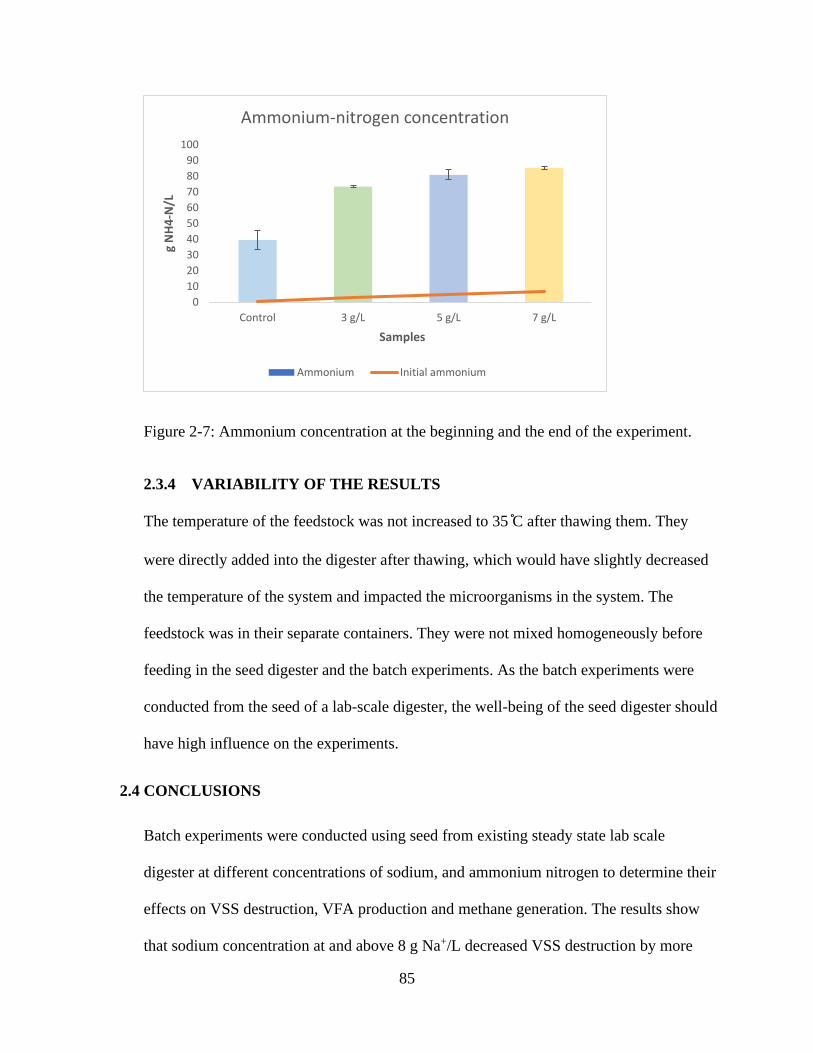
85

Figure 2-7: Ammonium concentration at the beginning and the end of the experiment.

2.3.4 VARIABILITY OF THE RESULTS

The temperature of the feedstock was not increased to 35 C after thawing them. They

were directly added into the digester after thawing, which would have slightly decreased

the temperature of the system and impacted the microorganisms in the system. The

feedstock was in their separate containers. They were not mixed homogeneously before

feeding in the seed digester and the batch experiments. As the batch experiments were

conducted from the seed of a lab-scale digester, the well-being of the seed digester should

have high influence on the experiments.

2.4 CONCLUSIONS

Batch experiments were conducted using seed from existing steady state lab scale

digester at different concentrations of sodium, and ammonium nitrogen to determine their

effects on VSS destruction, VFA production and methane generation. The results show

that sodium concentration at and above 8 g Na+/L decreased VSS destruction by more

0

10

20

30

40

50

60

70

80

90

100


g N

H4

-N/L

Samples

Ammonium-nitrogen concentration

Ammonium Initial ammonium

86

than 35% than control. Methane production reduced by 46% when the sodium

concentration was 10 g/L. NH4+-N concentrations of 5 g/L and above reduced methane

production by 71%, and VSS destruction by 3%, as compared to control batch. This

shows the salt and ammonia are toxic to the methanogens that are responsible for

producing methane from anaerobic digestion of organic waste.

87

BIBLIOGRAPHY

2015-2017 C-CAP Derived 10-meter Land Cover - BETA | ID: 57099 | InPort. (2019). Office for

Coastal Management. https://www.fisheries.noaa.gov/inport/item/57099

About ArcGIS Pro—ArcGIS Pro | Documentation. (n.d.). Retrieved October 19, 2020, from

https://pro.arcgis.com/en/pro-app/get-started/get-started.htm

About Us – LAWPCA. (n.d.). Retrieved July 25, 2020, from

http://www.lawpca.org/?page_id=237

Ali Shah, F., Mahmood, Q., Maroof Shah, M., Pervez, A., & Ahmad Asad, S. (2014). Microbial

ecology of anaerobic digesters: The key players of anaerobiosis. In The Scientific World

Journal (Vol. 2014). Hindawi Limited. https://doi.org/10.1155/2014/183752

Amani, T., Nosrati, M., & Sreekrishnan, T. R. (2010). Anaerobic digestion from the viewpoint of

microbiological, chemical, and operational aspects - A review. Environmental Reviews,

18(1), 255–278. https://doi.org/10.1139/A10-011

Anwar. (2016). Effect of sodium salt on anaerobic digestion of kitchen waste Naveed Anwar ,

Wen Wang , Jie Zhang , Yeqing Li , Chang Chen ,. 1865–1872.

https://doi.org/10.2166/wst.2016.035

APHA. (2017). Standard Methods for the Examination of Water and Wastewater.

https://doi.org/10.2105/SMWW.2882.216

ArcGIS pro. (n.d.). Calculate the travel time between origins and destinations with OD Cost

Matrix—ArcGIS Pro | Documentation. Retrieved October 11, 2020, from

https://pro.arcgis.com/en/pro-app/help/analysis/networks/od-cost-matrix-tutorial.htm

ArcGIS Pro. (2020). What is the Suitability Modeler?—ArcGIS Pro | Documentation.

https://pro.arcgis.com/en/pro-app/help/analysis/spatial-analyst/suitability-modeler/what-is-

the-suitability-modeler.htm

Bangor Daily News. (2020). Hampden waste plant puts operations on hold as it struggles to pay

bills. https://bangordailynews.com/2020/06/10/news/bangor/hampden-waste-plant-puts-

operations-on-hold-as-it-struggles-to-pay-bills/

COWI. (2004). Preliminary Impact Assessment for an Initiative on the Biological Treatment of

Biodegradable Waste Final Study Report.

Criner, K. G., & Blackmer, L. T. (2011). 2011-Maine-Residential-Waste-Characterization-

Study.

Dun & bradstreet. (2020). US Farm Data, Inc. Company Profile | Omaha, NE | Competitors,

Financials & Contacts - Dun & Bradstreet. https://www.dnb.com/business-

directory/company-profiles.us_farm_data_inc.c717d28716249bcf20e5fccebb5cd3f3.html

ecomaine. (2017). food waste Goes Back to the Farm in FY 2017.

88

EPA. (2015). Ag 101 | Agriculture | US EPA.

http://www.epa.gov/agriculture/ag101/index.html[7http://www.epa.gov/agriculture/ag101/i

ndex.html

EPA. (2019). Food Recovery Hierarchy | Sustainable Management of Food | US EPA.

https://www.epa.gov/sustainable-management-food/food-recovery-hierarchy

EPA Facility Registry Service. (n.d.). EPA Facility Registry Service (FRS): Wastewater

Treatment Plants. 2020. Retrieved September 18, 2020, from

https://edg.epa.gov/metadata/catalog/search/resource/details.page?uuid=%7B86C00471-

0D39-4352-B629-14E3C0E2D042%7D

Esri. (2020). How To: Create a slope map from contour lines in ArcGIS Pro.

https://support.esri.com/en/technical-article/000023285

Excess Food Opportunities Map. (n.d.). Retrieved July 11, 2020, from


Excess Food Opportunities- Technical Methodology. (2020). Excess Food Opportunities Map,

Version 2.1 - Technical Methodology. https://www.epa.gov/sustainable-management-food

Fiberight. (2018). Fiberight Maine – Fiberight, LLC – Leading the Way Forward.

https://fiberight.com/fiberight-maine/

Fulford, D. (2015). Small-scale rural biogas programmes : a handbook.

How It Works | EAE – Exeter Agri-Energy. (n.d.). Retrieved July 25, 2020, from

http://www.exeteragrienergy.com/how-it-works/

Isenhour, C., Blackmer, T., Wagner, T., Silka, L., & Peckenham, J. (2016). Moving up the Waste

Hierarchy in Maine: Learning from “Best Practice” State-Level Policy for Waste

Reduction and Recovery Part of the Environmental Policy Commons, and the Natural

Resources Management and Policy Commons Repository Citation.

https://digitalcommons.library.umaine.edu/mitchellcenter_pubs

Karimini, A. R., Mehrdadi, N., Hashemian, S. J., Nabi Bidhendi, G. R., & Tavakkoli

Moghaddam, R. (2011). Selection of wastewater treatment process based on the analytical

hierarchy process and fuzzy analytical hierarchy process methods.

Kim, H. W., Nam, J. Y., Kang, S. T., Kim, D. H., Jung, K. W., & Shin, H. S. (2012). Hydrolytic

activities of extracellular enzymes in thermophilic and mesophilic anaerobic sequencing-

batch reactors treating organic fractions of municipal solid wastes. Bioresource Technology,

110, 130–134. https://doi.org/10.1016/j.biortech.2012.01.146

Layer: All Composting Facilities (ID: 22). (2018).

https://gispub.epa.gov/arcgis/rest/services/Region9/LND2003987_ExcessFoodRecipient/Ma

pServer/22

Leal, J. E. (2020). AHP-express: A simplified version of the analytical hierarchy process method.

MethodsX, 7. https://doi.org/10.1016/j.mex.2019.11.021

89

Maine DEP. (2017). Report to the Joint Standing Committee on the Environment and Natural

Resources 128 th Legislature, First Session MAINE DEPARTMENT OF

ENVIRONMENTAL PROTECTION Maine Solid Waste Generation and Disposal Capacity

Report: Calendar Year 2015 Contents. www.maine.gov/dep

Maine DEP. (2020). ACTIVE/LICENSED TRANSFER STATIONS Maine Department of

Environmental Protection.

Metcalf & Eddy. (2003). Wastewater Engineering Treatment and Reuse (H. D. S. George

Tchobanoglous, Franklin L. Burton, Ed.; 4th ed.). McGraw-Hill.

Mir, M. A., Hussain, A., & Verma, C. (2016). Design considerations and operational

performance of anaerobic digester: A review. Cogent Engineering, 3(1), 1–20.

https://doi.org/10.1080/23311916.2016.1181696

Mohee, R., & Mudhoo, A. (2012). Bioremediation and Sustainability : Research and

Applications. John Wiley & Sons, Incorporated.

http://ebookcentral.proquest.com/lib/umaine/detail.action?docID=861796

MRC Inc. (2018a). Facility | Municipal Review Committee. https://www.mrcmaine.org/fiberight/

MRC Inc. (2018b). MRC Members | Municipal Review Committee.

https://www.mrcmaine.org/municipalities/

Narihiro, T., & Sekiguchi, Y. (2007). Microbial communities in anaerobic digestion processes

for waste and wastewater treatment: a microbiological update. Current Opinion in

Biotechnology, 18(3), 273–278. https://doi.org/10.1016/j.copbio.2007.04.003

National Sewage Sludge. (2020). PFASinBiosolidsdocx-formatted.

Nazari, A., Salarirad, M. M., & Bazzazi, A. A. (2012). Landfill site selection by decision-making

tools based on fuzzy multi-attribute decision-making method. Environmental Earth

Sciences, 65(6), 1631–1642. https://doi.org/10.1007/s12665-011-1137-2

NRCM. (2016a). Maine Composting Companies - Natural Resources Council of Maine.

https://www.nrcm.org/sustainability/maine-composting-companies/

NRCM. (2016b). Maine Composting Companies - Natural Resources Council of Maine.

https://www.nrcm.org/sustainability/maine-composting-companies/

Pennington. (2018). Anaerobic Digestion Facilities Processing Food Waste in the United States

in 2015.

Pennington. (2019). Anaerobic Digestion Facilities Processing Food Waste in the United States

in 2016.

Public Law Chapter 461. (n.d.). PUBLIC Law, Chapter 461, An Act To Create a Sustainable

Solution to the Handling, Management and Disposal of Solid Waste in the State. Retrieved

November 13, 2020, from

https://www.mainelegislature.org/legis/bills/bills_127th/chapters/PUBLIC461.asp

90

Raju, C. S., Løkke, M. M., Sutaryo, S., Ward, A. J., & Møller, H. B. (2012). NIR monitoring of

ammonia in anaerobic digesters using a diffuse reflectance probe. Sensors, 12(2), 2340–

2350. https://doi.org/10.3390/s120202340

Seiple, T. E., Coleman, A. M., & Skaggs, R. L. (2017). Municipal wastewater sludge as a

sustainable bioresource in the United States. Journal of Environmental Management, 197,

673–680. https://doi.org/10.1016/j.jenvman.2017.04.032

Solid, M., Anderson, L., & Bergeron, M. (2016). Report to the Joint Standing Committee on the

Environment and Natural Resources 127 th Legislature, Second Session MAINE

DEPARTMENT OF ENVIRONMENTAL PROTECTION Contents. www.maine.gov/dep

Song, B., & Kang, S. (2016). A Method of Assigning Weights Using a Ranking and

Nonhierarchy Comparison. Advances in Decision Sciences, 2016.

https://doi.org/10.1155/2016/8963214

Stentiford, E., & de Bertoldi, M. (2010). Composting: Process.

http://ebookcentral.proquest.com’,’_blank’

Swan, R. M., Crook, B., & Gilbert, J. (2002). Microbial Emissions from Composting Sites.

http://ebookcentral.proquest.com’,’_blank’

Tzeng, G.-H., & Huang, J.-J. (2011). Multiple Attribute Decision Making : Methods and

Applications. CRC Press LLC.


Undersander, D., Cosgrove, D., Cullen, E., Grau, C., Rice, M. E., Renz, M., Sheaffer, C.,

Shewmaker, G., & Sulc, M. (2011). Alfalfa Management Guide ii Alfalfa Management

Guide. www.soils.org

Urban, R. C., & Isaac, R. de L. (2018). WTP and WWTP sludge management: a case study in the

metropolitan area of Campinas, southeastern Brazil. Environmental Monitoring and

Assessment, 190(10), 584. https://doi.org/10.1007/s10661-018-6972-0

US EPA. (2018). Basic Information on PFAS. https://www.epa.gov/pfas/basic-information-pfas

US EPA. (2020). Sustainable Management of Food Basics | Sustainable Management of Food |

US EPA. https://www.epa.gov/sustainable-management-food/sustainable-management-

food-basics

US EPA, OAR. (n.d.). AgSTAR Data and Trends. Retrieved October 2, 2020, from

https://www.epa.gov/agstar/agstar-data-and-trends

US EPA, OLEM. (n.d.). National Overview: Facts and Figures on Materials, Wastes and

Recycling. Retrieved October 2, 2020, from https://www.epa.gov/facts-and-figures-about-

materials-waste-and-recycling/national-overview-facts-and-figures-materials

US Farm Data. (2020). United States Farmers, Ranchers | Farm Mailing Lists, Ag Business

Leads - US Farm Data. https://www.usfarmdata.com/

USDA, & Natural Resource Conservation Service. (1995). Animal Manure Management.

https://www.nrcs.usda.gov/wps/portal/nrcs/detail/null/?cid=nrcs143_014211

91

Wall, J. D., Harwood, C. S., & Demain, A. L. (Arnold L. ). (2008). Bioenergy. ASM Press.

Williams, P. T., Roberts, R. D., Strange, K., Gladding, T. L., Gilbert, E. J., Crook, B., Redfearn,

A., Rabl, A., Spadaro, J. v, & Dolk, H. (2002). Environmental and Health Impact of Solid

Waste Management Activities. Royal Society of Chemistry.


Wisconsin Department of Natural Resources. (1992). Introduction to Anaerobic Digestion Study

Guide Wisconsin Department of Natural Resources Introduction to Anaerobic Digestion

Study Guide-June 1992 Edition. http://dnr.wi.gov

Xu, D. Y., Lin, Z. Y., Gordon, M. P. R., Robinson, N. K. L., & Harder, M. K. (2016). Perceived

key elements of a successful residential food waste sorting program in urban apartments:

stakeholder views. Journal of Cleaner Production, 134(Part A), 362–370.

https://doi.org/10.1016/j.jclepro.2015.12.107

92

CHAPTER 3 APPENDICES

3.1 APPENDIX A: SUITABILITY MAPS

3.1.1 MAINE

Figure 3-1: Suitability map of Maine.

93

3.1.2 NORTHERN REGION

Figure 3-2: Suitability map of Northern region.

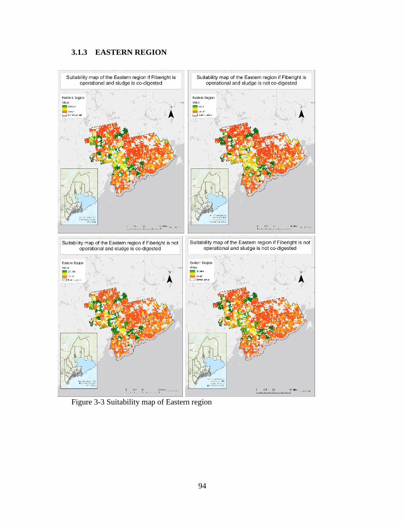
94

3.1.3 EASTERN REGION

Figure 3-3 Suitability map of Eastern region

95

3.1.4 MID-COAST REGION

Figure 3-4: Suitability map of Mid-Coast region

96

3.1.5 SOUTHERN REGION

Figure 3-5: Suitability map of Southern region

97

3.1.6 WESTERN REGION

Figure 3-6: Suitability map of the Western region

98

3.2 APPENDIX B: CRITERIA WEIGHTS BY AHP

3.2.1 ECONOMIC FACTORS

3.2.1.1 Sludge exclusion

Table 3-1: Assigned AHP numbers to economic factors in sludge exclusion

A1 A2

A1 1 2

A2 0.5 1

sum 1.5 3

Table 3-2: Normalized matrix for sludge exclusion

Normalized

A1 A2 Criteria Weights

A1 0.67 0.67 0.67

A2 0.33 0.33 0.33

sum 1.00 1.00 1.00

Table 3-3: Consistency Index for sludge exclusion

A1 A2 Criteria Weights Eigen value

A1 0.67 0.67 0.67 1.333333333

A2 0.33 0.33 0.33 0.666666667

sum 1 1 1 2

Consistency Index 0

99

3.2.1.2 Sludge Inclusion

Table 3-4: AHP numbers assigned to sludge inclusion

A1 A2 A3

A1 1 2 2

A2 0.5 1 2

A3 0.5 0.5 1

sum 2 3.5 5

Table 3-5: Normalized matrix for sludge exclusion

A1 A2 A3 Criteria Weights

A1 0.5 0.571429 0.4 0.490476

A2 0.25 0.285714 0.4 0.311905

A3 0.25 0.142857 0.2 0.197619

sum 1 1 1 1

Table 3-6: Consistency Index for sludge exclusion

A1 A2 A3 Criteria Weights

A1 0.490476 0.62381 0.395238 0.490476 1.509524 3.07767

A2 0.245238 0.311905 0.395238 0.311905 0.952381 3.053435

A3 0.245238 0.155952 0.197619 0.197619 0.59881 3.03012

sum 0.980952 1.091667 0.988095 1 3.053742

Consistency Index 0.026871

100

3.2.2 TECHNICAL FACTORS

Table 3-7: AHP numbers assigned to technical factors

B1 B2 B3

B1 1 5 3

B2 0.2 1 0.5

B3 0.333333 2 1

sum 1.533333 8 4.5

Table 3-8: Normalized matrix for technical factors

Normalized

B1 B2 B3 Criteria Weights

B1 0.652174 0.625 0.666667 0.647947

B2 0.130435 0.125 0.111111 0.122182

B3 0.217391 0.25 0.222222 0.229871

Table 3-9: Consistency Index for technical factors

B1 B2 B3 Criteria Weights

B1 0.647947 0.61091 0.689614 0.647947 1.94847 3.007145

B2 0.129589 0.122182 0.114936 0.122182 0.366707 3.001318

B3 0.215982 0.244364 0.229871 0.229871 0.690217 3.002627

3.003697

Consistency Index 0.001848

101

3.2.3 ENVIRONMENTAL FACTORS

Table 3-10: AHP numbers assigned to environmental factors

C1 C2

C1 1 2

C2 0.5 1

Sum 1.5 3

Table 3-11: Normalized matrix for environmental factors

C1 C2 Criteria Weights

C1 0.67 0.67 0.67

C2 0.33 0.33 0.33

sum 1 1 1

Table 3-12: Consistency Index for environmental factors

C1 C2 Criteria Weights

C1 0.67 0.67 0.67 1.33 2

C2 0.33 0.33 0.33 0.67 2

sum 1 1 1 2

0

102

Table 3-13: Criteria weights for sludge exclusion (Case 1)

Global

Factors

Global

Weigh

t Criteria

Symbo

l

Sludge Exclusion Transformati

ve weight in

Modeler Local

Weight

s

Global

Weight

s

Economical 0.24

Transportatio

n Cost A1 0.67 0.160

3

Food Waste


1.5

Sludge

Availability A3 - -

-

Technical 0.6

Airports B1 0.65 0.389 7.29

Land Cover B2 0.12 0.073 1.37

Slope B3 0.23 0.138 2.59

Environment

al 0.16

Sensitive

Areas C1 0.67 0.107

2

Residential

Areas C2 0.33 0.053

1

Sum 1 3 1 18.75

Table 3-14: Criteria Weights for the sludge inclusion (Case 1)

Global

Factors

Global

Weigh

t Criteria

Symbo

l

Sludge Inclusion Transformati

ve weight in

Modeler Local

Weight

s

Global

Weight

s

Economical 0.24

Transportatio

n Cost A1 0.49 0.118

2.48

Food Waste


1.58

Sludge


1

Technical 0.6

Airports B1 0.65 0.389 8.2

Land Cover B2 0.12 0.073 1.55

Slope B3 0.23 0.138 2.91

Environment

al 0.16

Sensitive

Areas C1 0.67 0.107

2.25

Residential

Areas C2 0.33 0.053

1.12

Sum 1 3 1 21.08

103

3.3 APPENDIX C: CALIBRATION CHARTS

Figure 3-7: Calibration chart for conductivity. Different known concentrations of sodium

were used to find the conductivity. This chart is used to calculate the actual sodium salt

concentration in samples

Figure 3-8: Calibration chart for ammonium concentration

y = 4.4409x + 1.5255R² = 0.9983

0

10

20

30

40

50

60

0 2 4 6 8 10 12

Co

nd

uct

ivit

y (u

s/cm

)

Sodium Ion Concentration (g/L)

Calibration Chart for Conductivity

104

3.4 APPENDIX D: SODIUM EXPERIMENT

105

Figure 3-9: Experimental pictures for salt toxicity test. The top left image represents the

samples ready to be clamped and incubated. The bottom left represents the sample in an

aluminum dish prepared to put in the oven for VS

measurement. The bottom right picture shows the alkalinity test.

3.5 APPENDIX D: AMMONIA EXPERIMENT

106

Figure 3-10: The top left picture represents the pre-autoclaved labeled serum bottles just

before the experiment. The top right image represents the flushing of nitrogen gas into

the batch after the addition of feed. The bottom right shows the labeled vials for the

HPLC samples

Figure 3-11: The seed digester. The primary digester is in the water bath, and the water

displacement method is used to measure the volume of the gas

107

CHAPTER 4

BIOGRAPHY OF THE AUTHOR

Usha Humagain, was born in a small village near Kathmandu, Nepal, in 1993. She

graduated high school from SOS Village, Bharatpur, in 2011 and joined Tribhuvan

University for her undergraduate degree in Civil Engineering. During her undergraduate

project, she studied the status of wastewater management in Pokhara, Nepal. She

conducted different lab tests and analyzed the drainage system. In April 2015, during the

earthquake, she volunteered for Nepal Government to determine the earthquake risk

assessment in Thumki V.D.C of Kaski. She was actively involved in student clubs during

her college days.

After graduation in 2015, she started working full time for a consulting firm, S.W. Nepal

Pvt. Ltd., in Kathmandu as a Rural Infrastructure Engineer. She worked for USAID

Sajheedari Bikaas Project from Dec 2015- Dec 2017 by constructing and rehabilitating

small scale drinking water projects, community centers, and roads through the firm. She

has also worked for OXFAM to monitor its drinking water projects, household profiling,

and severity mapping of Nepal's flood-affected districts. She has worked for Concern

Worldwide through the consulting firm to provide technical oversight of school

construction in three districts- Sindhuli, Ramechhap, and Dhading. She was involved in

different small-scale projects like lime stabilization tests with Bee Rowan, training the

sub-engineers and overseers on small scale projects through the Karnali Employment

program, constructing a bamboo school, surveying and estimating on the widening of the

Ranibari trail.

108

In fall 2018, she pursued her masters at the University of Maine in Civil Engineering.

Usha has a high interest in traveling the rural regions of Nepal and understanding

people's lives. She will be working again in Nepal after receiving her degree. Usha is a

candidate for the Master of Science degree in Civil Engineering from the University of

Maine in December 2020.

use of gis to find optimum locations for anaerobic

Documents