use of ground penetrating radar for construction quality ... · 3 1. report no. p307 2. government...

Use of Ground Penetrating Radar for Construction

Quality Assurance of Concrete Pavement

NDOR Project Number P307

November 2009

2


Quality Assurance of Concrete Pavement

NDOR Project Number P307

FINAL REPORT

PRINCIPAL INVESTIGATORS

George Morcous, Ph.D., PE.

Ece Erdogmus, Ph.D.

SPONSORED BY

Nebraska Department of Roads

University of Nebraska - Lincoln

November 2009

3

1. Report No.

P307

2. Government Accession No.

3. Recipient’s Catalog No.

1. Title and Subtitle


2. Report Date

November, 2009

Quality Assurance of Concrete Pavement 3. Performing Organization Code

4. Author(s)

George Morcous and Ece Erdogmus

5. Performing Organization Report

No.

6. Performing Organization Name and Address 7. Work Unit No.

University of Nebraska-Lincoln

1110 South 67th

St.

Omaha, Nebraska 68182-0178

8. Contract or Grant No.

9. Sponsoring Agency Name and Address

University of Nebraska – Lincoln

10. Type of Report and Period Covered

Final Report

P. O. Box 94759, Lincoln, NE 68509-4759

11. Sponsoring Agency Code

12. Supplementary Notes

Abstract: Extracting concrete cores is the most common method for measuring the thickness of concrete

pavement for construction quality control. Although this method provides a relatively accurate thickness

measurement, it is destructive, labor intensive, and time consuming. Moreover, concrete cores are usually taken

approximately every 750 ft, which may be inadequate for estimating the actual thickness profile of a pavement

section; however extracting more cores would damage the pavement extensively and increase the labor cost and

time excessively. Ground Penetrating Radar (GPR) is a well-established technique for subsurface exploration.

Recently, GPR has been used for several transportation applications, such as measuring layer thickness in asphalt

pavement, locating reinforcing bars and tendons, and detecting deteriorations and anomalies in concrete structures.

The main advantages of GPR are speed, accuracy, and cost-effectiveness when scans are conducted on large areas.

The objective of this project is to investigate the accuracy and cost-effectiveness of using GPR for

measuring the thickness of concrete pavement for quality assurance purposes. The GPR systems GSSI SIR20 and

SIR3000 with a high resolution 1.6 MHz ground coupled antenna were used in measuring the thickness of concrete

pavement up to 14 inch thick. Several laboratory and field tests have been carried out to determine the accuracy of

the GPR measurement at different concrete ages and when various metal artifacts are used underneath the concrete

to improve the reflectivity of the bottom surface. Testing results have indicated that GPR is a cost-effective non-

destructive technique for measuring the thickness of concrete pavement, compared to extracting concrete cores,

and an accuracy of 1/8 in can be achieved when appropriate reflectors and calibration cores are used. 13. Keywords: GPR, Concrete Pavement

Thickness.

14. Distribution Statement

15. Security Classification

(of this report)

Unclassified

16. Security Classification (of

this page)

Unclassified

17. No. of

Pages

70

22. Price

4

DISCLAIMER

This report was funded in part through grant[s] from the Federal Highway Administration

[and Federal Transit Administration], U.S. Department of Transportation. The views and

opinions of the authors [or agency] expressed herein do not necessarily state or reflect those of

the U. S. Department of Transportation. The contents of this report reflect the views of the

authors who are responsible for the facts and the accuracy of the data presented herein. The

contents do not necessarily reflect the official views or policies of the Nebraska Department of

Roads, nor the University of Nebraska-Lincoln. This report does not constitute a standard,

specification, or regulation. Trade or manufacturers’ names, which may appear in this report, are

cited only because they are considered essential to the objectives of the report. The United

States (U.S.) government and the State of Nebraska do not endorse products or manufacturers.

5

ACKNOWLEDGEMENTS

This project was sponsored by the Nebraska Department of Roads (NDOR) and the

University of Nebraska-Lincoln. The support of the technical advisory committee (TAC)

members is gratefully acknowledged. They spent a lot of time and effort in coordinating this

project, discussing its technical direction, and inspiring the university researchers.

Acknowledgement also goes to the following undergraduate and graduate students who

participated in the different tasks of the project:

1. Videgla Sekpe

2. Steve Cross

3. Regina Song

4. Michel Shafik

5. Catherine K. Armwood

6. Mary Naughtin

7. Kenzi Meyer

8. Eliya Henin

6

ABSTRACT

Extracting concrete cores is the most common method for measuring the thickness of

concrete pavement for construction quality control. Although this method provides a relatively

accurate thickness measurement, it is destructive, labor intensive, and time consuming.

Moreover, concrete cores are usually taken approximately every 750 ft, which may be

inadequate for estimating the actual thickness profile of a pavement section; however extracting

more cores would damage the pavement extensively and increase the labor cost and time

excessively. Ground Penetrating Radar (GPR) is a well-established technique for subsurface

exploration. Recently, GPR has been used for several transportation applications, such as

measuring layer thickness in asphalt pavement, locating reinforcing bars and tendons, and

detecting deteriorations and anomalies in concrete structures. The main advantages of GPR are

speed, accuracy, and cost-effectiveness when scans are conducted on large areas.

The objective of this project is to investigate the accuracy and cost-effectiveness of using

GPR for measuring the thickness of concrete pavement for quality assurance purposes. The GPR

systems GSSI SIR20 and SIR3000 with a high resolution 1.6 MHz ground coupled antenna were

used in measuring the thickness of concrete pavement up to 14 inch thick. Several laboratory and

field tests have been carried out to determine the accuracy of the GPR measurement at different

concrete ages and when various metal artifacts are used underneath the concrete to improve the

reflectivity of the bottom surface. Testing results have indicated that GPR is cost-effective non-

destructive technique for measuring the thickness of concrete pavement, compared to core

extraction, and an accuracy of 1/8 in. can be achieved when appropriate reflectors and calibration

cores are used.

7

TABLE OF CONTENTS

1. INTRODUCTION ..................................................................................................................11

1.1 BACKGROUND ............................................................................................................11

1.2 OBJECTIVES .................................................................................................................12

2. LITERATURE REVIEW .......................................................................................................13

2.1 GPR METHODOLOGY .................................................................................................13

2. 2. USE OF GPR FOR PAVEMENT LAYER THICKNESS MEASUREMENTS ........16

3. LABORATORY TESTS ........................................................................................................20

3.1 LAB TEST # 1 ................................................................................................................20

3.2 LAB TEST # 2 ................................................................................................................25

4. FIELD TESTS ........................................................................................................................36

4.1 FIELD TEST # 1 .............................................................................................................36

4.2 FIELD TEST # 2 .............................................................................................................40

4.3 FIELD TEST # 3 .............................................................................................................45

4.4 FIELD TEST #4 ………………………………………………………………………. 49

4.5 FIELD TEST #5 ………………………………………………………………………. 53

5. BENEFIT-COST ANALYSIS ................................................................................................55

6. SUMMARY AND CONCLUSIONS .....................................................................................58

7. IMPLEMENTATION PLAN …………………………………………………………….... 60

8. REFERENCES .......................................................................................................................61

APPENDIX A .............................................................................................................................62

8

LIST OF FIGURES

Figure 1.1: Core Measuring Apparatus

Figure 2.1: GPR Principles

Figure 2.2: GPR survey of concrete pavement (Maierhofer 2003)

Figure 2.3: Reinforced Concrete Slabs Used for GPR Testing at PKI labs by authors

Figure 3.1 Metal ring placed underneath a 12 in. thick concrete slab

Figure 3.2 GPR grid scan of the 12 in. thick concrete slab

Figure 3.3 Projection views of the tested slab

Figure 3.4 GPR signle reflections at the reinforcing bars and metal ring

Figure 3.5 GPR signle reflections at the reinforcing bars, metal ring, and metal strip

Figure 3.6 Form ties used in the lab test # 1

Figure 3.7 GPR signal reflections at the reinforcing bars and form tie

Figure 3.8 Location of the driveway built for lab test # 2

Figure 3.9 The five metal objects used in lab test # 2

Figure 3.10 Location of the five metal objects used in lab test # 2

Figure 3.11 Radargram of the scan perfomed on 12/21/2007



Figure 3.14 Average concrete thickness versus concrete age

Figure 3.15 GPR grid scan of the test driveway

Figure 3.16 Thickness measurement using extracted cores

Figure 3.18 Radargram of scan performed at the plate location

Figure 3.19 Radargram of scan performed at the T Sec. location

Figure 3.20 Radargram of scan performed at the right-side tie location

Figure 3.22 Movement of the lef-side tie from its original location

Figure 3.23 Comparing thickness measurement using cores and GPR

Figure 4.1 GPR scan using SIR 3000 system on highway I-275

Figure 4.2 Radargram at Station 322 + 43



9

Figure 4.5 Grid setup at station 325 + 12

Figure 4.6 Grid used for scan # 1

Figure 4.7 Radargram of the x-direction scans (Scan #1)

Figure 4.8 Radargram of the y-direction scans (Scan #1)

Figure 4.9 Marked and detected locations of the metal ring on the grid of scan #1





Figure 4.14 Location of the GPR scanned concrete pavement on Highway 30 in Fremont, NE

Figure 4.15 Steel plate placed underneath the concrete pavement

Figure 4.16 Grid scan at the marked location of the steel plate

Figure 4.17 Radargram of the GPR grid scan at one station in field test # 3

Figure 4.18 Location of the GPR scanned concrete pavement on Hwy 2, Lincoln, NE

Figure 4.19 Placing reflector disks before paving Hwy 2

Figure 4.20 Grid scan at the marked location of the steel disk

Figure 4.21 Radargram (wiggle mode) of the GPR grid scan at plate # 15

Figure 4.22 Location of the GPR scanned concrete pavement on I-80, Lincoln, NE

Figure 4.23 Placing reflector disk before paving I-80



10

LIST OF TABLES

Table 2.1: Relative permittivity of different material at a frequency of 1 GHz

Table 3.1 Number and dimensions of the metal objects used in lab test # 2

Table 3.2 Concrete Mix used in lab test # 2

Table 3.3 Results of GPR thickness measurments at different concrete ages

Table 3.4 Difference in thickness measurment usinf cores and GPR

Table 4.1 Stations and the corresponding core thickness

Table 4.2 Locations of plates scanned in field test #3

Table 4.3 Results of field test #3

Table 4.4 Locations of the 24 disks used in Hwy 2 project

Table 4.5 Results of field test #4a

Table 4.6 Results of field test #4b

Table 4.7 Locations of the 22 disks used in I-80 project


Table 5.1. Benefit-Cost Comparison Between GPR and Coring

11

1. INTRODUCTION

Nebraska Department of Roads (NDOR) performs routine quality checks on their

concrete pavement projects. This process is time consuming and costly endeavor with the current

destructive method of coring. Therefore, a nondestructive, accurate, cost-effective, and speedy

method can benefit the state. In this project, feasibility and accuracy of using Ground Penetrating

Radar (GPR) for concrete pavement thickness quality assurance is studied through a systematic

research methodology including review of literature, case studies testing various methodologies,

and a cost-benefit analysis. Results of the study are presented in this report.

1.1. Background

Determining the thickness of concrete pavement is an important consideration for

construction quality assurance of new pavements and structural capacity estimation of existing

pavements. This information is essential for pavement management systems in order to maintain

the safety, serviceability, and durability of pavement networks.

Currently, NDOR measures the thickness of concrete pavement using drilled cores and

steel measuring devices. If the cores are in question, the ASTM C174 laboratory test method is

adopted. Pavement cores are extracted every 750 ft and taken to the lab to determine the

compliance of concrete construction with design specifications. The three-point callipering

device shown in Figure 1.1 is used to make length measurement at the center of the specimen

and at eight additional points equally spaced along the circumference of the specimen (ASTM

2006a). The average of the nine measurements expressed to the nearest 0.1” is reported as the

length of the concrete core.

Figure 1.1: Core Measuring Apparatus

12

Although this procedure results in relatively accurate thickness measurements of concrete

pavement, it provides local information as cores are required to be extracted every 750 ft,

therefore it is limited. In addition, core extraction is a time consuming, laborious, and destructive

process. Moreover, the integrity of the pavement is already obstructed with the drilling and later-

filling process.

1.2. Objectives

Given the drawbacks of the coring method discussed in the previous section, it is evident

that a nondestructive alternative for pavement thickness measurements, which provides

continuous information along the pavement section in a rapid and cost effective manner, can

save NDOR time, money and provide the department with the possibility of continuous quality

control on pavement contracts. The investigators propose that the ground penetrating radar

(GPR) technology offers a solution to this need if a practical procedure overcoming the

limitations is developed. Thus the objectives of this research project are:

General

Investigate the feasibility of using GPR on a routine basis for measuring the

thickness of concrete pavement.

Specific

Determine the accuracy of GPR in measuring the thickness of concrete pavement

using “verification cores”

Investigate the effect of various parameters on GPR accuracy, such as pavement

age and thickness.

Identify the optimum number of “calibration cores” required to achieve the target

accuracy.

Evaluate the repeatability of GPR in thickness measurement.

13

2. LITERATURE REVIEW

2. 1. GPR Methodology

The ground penetrating radar (GPR) method involves the transmission of electromagnetic

waves into the material under investigation. The reflections of these waves at interfaces and

objects within the material are analyzed to determine the location (horizontal distance from a

reference point) and depth (vertical distance from the surface) of the detected interfaces and

buried objects. GPR can also be used to differentiate layers of material and to determine certain

properties of the materials, such as their dielectric constants or conductivity for electromagnetic

waves.

There are two basic types of radar waves: pulse and continuous wave. The pulse radar

transmits a burst of radar energy and then waits for the energy (or echo) to be reflected back to

the same antenna. The continuous radar wave, on the other hand, transmits a constant beam of

energy that returns to a separate antenna when it meets a moving object (such as an aircraft or a

car). The returned wave has a frequency that is slightly higher (if the object is moving toward the

radar) or lower (if the object is moving away from the radar) than the frequency of the original

wave. By measuring this change in frequency, the speed of the object can be determined.

GPR is the propagation of short pulse radar waves (pulse duration less than 1 ns) through the

layers of materials under investigation. Figure 2.1 shows a radar signal that is emitted via an

antenna into a structure composed of three different materials. Signals are reflected at the

interfaces between the materials and their interfaces with the surrounding medium. Reflected

signals are received by the same antenna to present one scan or trace. Several scans are taken at

different locations on the investigated structure and their data are recorded in the storage device

of the central unit. These data are then processed and displayed on a monitor for further analysis

(manual or automatic interpretation). Analyzed GPR data can reveal significant information

about the materials within the structure (e.g. conductivity, etc…) and their condition (eg: layers

and anomalies within the structure, etc…).

14

Figure 2.1: GPR Principles

From the electromagnetic standpoint, materials can be categorized as follows: a) metallic,

and b) dielectric. Metallic materials have high conductivity and attenuate electromagnetic waves

to a great extent resulting in shallow penetration, while dielectric materials have low

conductivity and attenuate electromagnetic waves to a limited extent resulting in deep

penetration. The relative dielectric constant of a particular material (εr, sometimes called relative

permittivity) is the ratio of permittivity of the material to permittivity of vacuum (ε0 = 8.854 x 10-

12 F/m). Although the transition from metallic to dielectric is gradual, this relative permittivity is

used to indicate the nature of the material (high value for metallic and low value for dielectric).

Table 1 lists the relative permittivity of different materials at an electromagnetic frequency of 1

GHz.

Table 2.1: Relative permittivity of different material at a frequency of 1 GHz (Table by GSSI, a

major GPR manufacturer in the U.S.)

Material Relative Permittivity

Air 1

Dry Masonry 3-5

Moist Masonry 5-26

Dry Concrete 5-8

Moist Concrete 8-16

Asphalt 3-5

Granite 5-7

Basalt 8

PVC 3

Water 81

Ice 4-8

15

ro

or

rr

rr

mz

RT

zz

zzR

1

12

12

The propagation velocity (υ) of a transmitted radar signal through a material is a function of its

relative permittivity (εr) and relative magnetic permeability (mr) as follows:

rr m

c

[1]

In low-loss materials, as most of the dielectric materials, the relative magnetic permeability (mr)

can be assumed to be unity. Therefore, if the relative permittivity of the material under

investigation is known, the propagation velocity can be calculated using Equation 1. The

propagation velocity of the waves within specific materials is then used to determine the

thickness of each material layer using the two-way travel time recorded by the GPR antenna. The

difference in time between the reflected signals at the top and bottom interfaces of the layer

times the velocity gives the distance traveled by the wave, i.e. the thickness of the layer. It

should be noted that relative permittivity of a material is frequency-dependent and is influenced

by several parameters, such as the temperature, moisture, and salt content of the material. These

parameters have to be considered through calibration before calculating the velocity in order to

obtain accurate thickness measurements.

When the incident signal meets the interface between two materials with different

dielectric constants, part of the incident energy is reflected, while the other part is transmitted.

The amount of reflected and transmitted energy is determined by the reflection and transmission

coefficients (R and T) respectively. These coefficients are dependent on the relative impedance

of the two materials (zr1 , zr2), which are functions of the dielectric constant of the materials (εr1,

εr2). These coefficients are calculated as follows:

[2]

[3]

[4]

where mo = 4π * 10-7

H/m is the magnetic permeability of free space.

As can be deduced from equations 2, 3, and 4, the smaller the difference in the dielectric constant

of the two materials, the smaller the reflection coefficient and the larger the transmission

16

coefficient. This means that the change of amplitude of the energy (i.e. attenuation) reflected

from the interface between two materials is a good indicator of the properties of these materials.

As the incident energy continues to penetrate other materials and meets successive interfaces,

other reflections are sent back to the antenna and recorded over time to generate the waveform.

Measuring the time and amplitude of reflections (peaks or valleys) in the waveform facilitates

the determination of layer thicknesses (Eq. 1), depth of buried objects, and changes in material

properties (Eq. 2,3, and 4), which are the basic purposes of using the GPR technology.

2. 2. Use of GPR for Pavement Layer Thickness Measurements

Traditionally, highway engineers use drilled cores to obtain pavement samples for

laboratory testing to determine the thickness of different layers, examine the conditions that may

cause pavement deterioration, and select the most appropriate maintenance actions. Conventional

methods of core sampling are expensive and time-consuming because they are labor intensive

and require lane closure until all cores are drilled, checked and refilled, which affects the safety

of workers and the traveling public (FHWA 2004).

GPR has been used for a variety of applications relating to pavement evaluation, such as

determining pavement thickness, locating changes in pavement structure, detecting voids under

jointed concrete slabs, identifying location and orientation of dowels in jointed concrete

pavement, and spotting moisture and stripping within asphalt pavement (Maser 1996).

Several studies have been reported on using GPR to measure the thickness of pavement

layers. Loulizi et al. (2003) have conducted an experiment on a 150 meter long asphalt paved

secondary road and reported a percentage error of less than 3.6% between the measured

thickness and the GPR-predicted thickness. Al-Qadi and Lahouar (2004) have conducted a GPR

survey over a 40 meter long asphalt pavement section at the Virginia Smart Road and reported an

average layer thickness error of 2.9% compared to core thickness. Willett et al. (2006) have

conducted a study to evaluate the accuracy of GPR in measuring pavement layer thickness in

both asphalt and concrete pavement. This study has shown a significant increase in GPR

accuracy with increasing the number of calibration cores in asphalt and concrete pavement.

GPR surveys have also been used to control the embedded depth and the inclined position

of the dowels or anchors that are placed perpendicular to the transverse and longitudinal joints in

concrete pavements during construction (Maierhofer 2003). Errors in positioning these dowels

17

result in irregular concrete cracks and rapid joint deterioration. Figure 2.2 shows the GPR

waveform recorded using 1.5 GHz antenna close to a transverse joint. Interpreting this

information is used to locate each dowel and enabled quality control in pavement construction.

Data interpretation requires training, which is available by the GPR manufacturers with the

purchase of their equipment. In-house training and practice is also beneficial, where the

operators scan test specimens with known objects/layers and confirm the known variables with

the scan data.

Figure 2.2: GPR survey of concrete pavement (Maierhofer 2003)

Several techniques are available to estimate pavement thickness using GPR for the

department of transportation. Antennas can be used in two ways, air coupled and ground

coupled. An air coupled antenna unit can be mounted to the back of a moving vehicle and travel

at high speeds with the antenna between six and twenty inches above the pavement which does

reduce the depth of penetration. A ground coupled system antenna rests completely on the

ground and reduces the reflection from the top of the concrete, therefore increasing the depth of

penetration but reduces the speed of collection. Equation 1 can be used to estimate the thickness

of the pavement.

ir

ii

ctd

,2 (1)

Where di = the thickness of the layer

ti = the two way travel time of the signal through the layer

18

c = the speed of light

εr,,i = the dielectric constant of the layer

Using this equation the dielectric needs to be found using the calibration technique built

into the GPR and a strong reflection below the layer of concrete, possibly a metal plate that will

reflect all of the signal energy back to the antenna. This technique can also be applied to

pavement with multiple layers with slightly more complicated analysis. When this technique

was tested by Al-Qadi during thickness measurements of hot mix asphalt layers, an error of 2.9%

compared to measured core samples was recorded (Al-Qadi 2004).

A presentation at the 8th

international conference on GPR explained the use of vehicle

mounted radar scans as promising in both accuracy and speed of collection where data is

collected using two air-launched 1 GHz antennas suspended off of the rear of a vehicle bumper.

The system is calibrated by placing an aluminum plate on the surface of the ground and then to

start the radar system recording and driving away only after several scans have been recorded.

The model also assumes a smooth surface and homogenous pavement. The accuracy of this

method is better than commonly encountered in ASTM D3549 through coring and ASTM D4748

by short-pulse radar (Olhoeft 2000).

In a study conducted in Kentucky, the accuracy of thickness measurement using ground

penetrating radar on asphalt and concrete using a 1 GHz air launched horn antenna was measured

in a variety of environments. The relationship was then evaluated between data analyzed with

and without core samples taken. This study recommends the use of core samples to increase the

accuracy of depth measurement by using the core depths to calibrate the ground penetrating

radar. Four core samples is recommended to minimize the error of the ground penetrating radar,

but it does not mention for what length or area of concrete this number of cores is based on.

Overall, it is concluded that any addition of core samples to the GPR has a positive effect on the

accuracy of the scans. For concrete slabs the accuracy ranges between 1.66 inches and 0.01

inches for pavement thicknesses of 9 to 12 inches (Willet 2006).

A project for the Florida Department of Transportation was carried out to further develop

GPR techniques and capabilities to increase accuracy and to reduce post-processing and operator

interaction. A computer program named Thickness Evaluation of Roads by Radar, TERRA was

19

developed to automate the GPR process. Using this program and an air coupled antenna radar

vehicle showed a resulting error of only 0.30 inches compared to core samples (Kurtz 2001).

Research has been done utilizing many different types of GPR and post-processing

techniques to accurately measure the thickness of pavement by Al-Qadi et al. in 2001. They used

GPR to accurately measure the thickness of flexible pavement by calibrating the GPR at each

location through the use an aluminum sheet placed below grade. Two GPR systems were used

simultaneously, air-coupled and ground-coupled collected at 16 kph and 1 scan per 110 mm.

Cores were taken to verify the data with the average error being only 6.7%. Maser in 1996

measured as-built conditions of pavement using GPR and PAVLAYER software with an

accuracy of + 7.5%. Mesher et al. (1995) reported a project where a GPR system called “Road

Radar” was used to measure pavement thickness on three sites. The self calibrating system was

used with a 2.5 GHz antenna. Linear regression statistical analysis was used reporting an

average R2 value greater than 0.9 (Loulizi 2003).

The principal investigators of this project also carried out some relevant work before the

granting of the current project. An exploratory study was carried out by the PI using the

Structure Scan system to accurately measure the cover thickness in reinforced concrete slabs and

to precisely locate reinforcing bars. Figure 2.3 shows five 3 ft x 3 ft slabs with thickness ranging

from 6” to 12” prepared for testing at the Structures Laboratory at PKI, Omaha. Results of this

study are shown in Appendix A.

Figure 2.3: Reinforced Concrete Slabs Used for GPR Testing at PKI labs by authors

20

3. LABORATORY TESTS

Two laboratory tests were carried out to estimate the accuracy of measuring the thickness of

concrete pavement using GPR and to determine the most economical way to improve this

accuracy. The next two subsections describe the two tests in details.

3.1 Lab Test # 1

The first lab test was performed on Sept. 20, 2007 at the Peter Kiewit Institute (PKI) Structural

Laboratory, where the temperature is approximately 75oF and the relative humidity is

approximately 70%. In this test, a 3 ft x 3 ft x 12 in. reinforced concrete slab was placed on top

of 8 in. thick base layer made of 47B sand and gravel. The concrete of this slab is almost one and

half year old and it dielectric constant is assumed to be 6.25.

A 2 in. diameter metal ring was placed on the base layer as shown in Figure 3.1 before placing

the concrete slab. A 2 ft x 2ft grid was placed on the top surface of the slab and two GPR grid

scans were performed at 2 in. spacing as shown in Figure 3.2.

Figure 3.1 Metal ring placed underneath a 12 in. thick concrete slab

21

Figure 3.2 GPR grid scan of the 12 in. thick concrete slab

Figure 3.3 shows the plan, side view and elevation of the 12 in. thick reinforced concrete slab

and the location of the metal ring. The slab had a 4 in. deep saw cut at the middle and was

reinforced with 2#8 bars crossing the cut to simulate the dowel bars across the joints in concrete

pavements.

Figure 3.3 Projection views of the tested slab

22

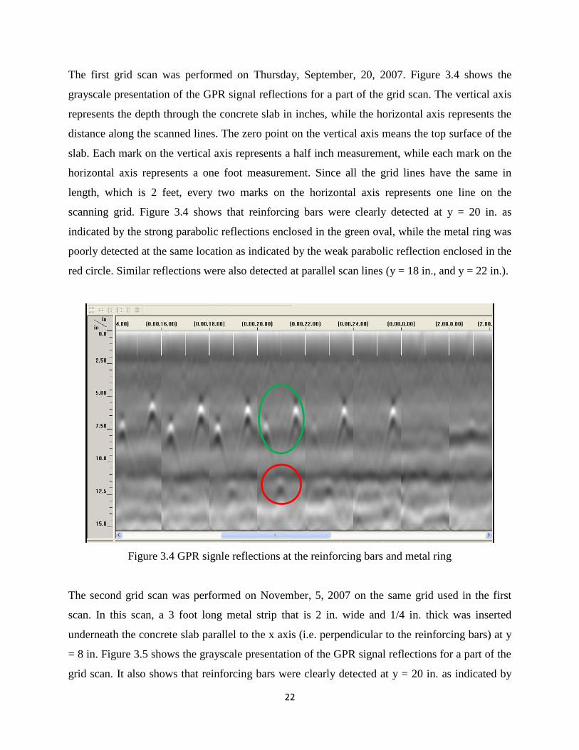
The first grid scan was performed on Thursday, September, 20, 2007. Figure 3.4 shows the

grayscale presentation of the GPR signal reflections for a part of the grid scan. The vertical axis

represents the depth through the concrete slab in inches, while the horizontal axis represents the

distance along the scanned lines. The zero point on the vertical axis means the top surface of the

slab. Each mark on the vertical axis represents a half inch measurement, while each mark on the

horizontal axis represents a one foot measurement. Since all the grid lines have the same in

length, which is 2 feet, every two marks on the horizontal axis represents one line on the

scanning grid. Figure 3.4 shows that reinforcing bars were clearly detected at y = 20 in. as

indicated by the strong parabolic reflections enclosed in the green oval, while the metal ring was

poorly detected at the same location as indicated by the weak parabolic reflection enclosed in the

red circle. Similar reflections were also detected at parallel scan lines (y = 18 in., and y = 22 in.).

Figure 3.4 GPR signle reflections at the reinforcing bars and metal ring

The second grid scan was performed on November, 5, 2007 on the same grid used in the first

scan. In this scan, a 3 foot long metal strip that is 2 in. wide and 1/4 in. thick was inserted

underneath the concrete slab parallel to the x axis (i.e. perpendicular to the reinforcing bars) at y

= 8 in. Figure 3.5 shows the grayscale presentation of the GPR signal reflections for a part of the

grid scan. It also shows that reinforcing bars were clearly detected at y = 20 in. as indicated by

23

the strong parabolic reflections enclosed in the green oval, while the metal ring was poorly

detected at the same location as indicated by the weaker parabolic reflection enclosed in the red

circle. The metal strip was also clearly detected at x = 0 as indicated by the strong parabolic

reflections enclosed in the yellow circle. By comparing these reflections, it can be concluded that

the strength (i.e. amplitude) of the reflected signals is directly proportional to the surface area of

the detected metal object.

Figure 3.5 GPR signle reflections at the reinforcing bars, metal ring, and metal strip

A third scan was performed on November 6, 2007 on the same concrete slab but using the line

scan instead of the grid scan. In this scan, a 20 in. long, 3/4 in. wide, and 1/8 in. thick form tie, as

shown in Figure 3.6, was inserted parallel to, and in between the two reinforcing bars. Figure 3.7

shows the grayscale presentation of the GPR signal reflections for a part of the line scan. This

figure shows that reinforcing bars were clearly detected as indicated by the strong parabolic

reflections enclosed in the green circle, while the form tie was less clearly detected as indicated

by the weaker parabolic reflection enclosed in the yellow circle. By comparing the two

reflections, the previous conclusion that the strength of the reflected signals is highly dependent

on the object surface area is confirmed.

24

Figure 3.6 Form ties used in the lab test # 1

Figure 3.7 GPR signal reflections at the reinforcing bars and form tie

25

3.2 Lab Test # 2

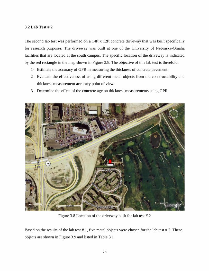
The second lab test was performed on a 14ft x 12ft concrete driveway that was built specifically

for research purposes. The driveway was built at one of the University of Nebraska-Omaha

facilities that are located at the south campus. The specific location of the driveway is indicated

by the red rectangle in the map shown in Figure 3.8. The objective of this lab test is threefold:

1- Estimate the accuracy of GPR in measuring the thickness of concrete pavement.

2- Evaluate the effectiveness of using different metal objects from the constructability and

thickness measurement accuracy point of view.

3- Determine the effect of the concrete age on thickness measurements using GPR.

Figure 3.8 Location of the driveway built for lab test # 2

Based on the results of the lab test # 1, five metal objects were chosen for the lab test # 2. These

objects are shown in Figure 3.9 and listed in Table 3.1

26

Figure 3.9 The five metal objects used in lab test # 2

Table 3.1 Number and dimensions of the metal objects used in lab test # 2

Object Number Dimension (in.)

T Sec. 1 1.5 x 1.5 x 33

L Sec. 1 1 x 1 x 34

Form Tie 2 20 x 3/4 x 1/8

Plate 1 6 x 6 x 1/8

The construction of the driveway started on November 19, 2007 by leveling the subgrade

through cut and fill operations using the existing soil and 47B sand and gravel. The subgrade was

leveled so that the thickness of the concrete pavement varies from 10 in. to 14 in. Then, three

sides of the driveway were formed using 2 x 12 lumbers, while the fourth side was formed by the

side of an existing driveway that is 14 in. thick. On December 3, 2007, the subgrade was

compacted using a mobile compactor and the five objects listed in table 4.1 were anchored to the

subgrade at the locations shown in Figure 3.10. It should be noted that the top of the figure is

pointing toward the South. On December 4, 2007, the concrete was poured, vibrated, finished,

and covered with foam planks for curing. Table 3.2 lists the design of the concrete mix used in

this application, which is one of NDOR standard mixes specified for pavement construction.

Photos of the various construction steps are provided in Appendix A.

27

Figure 3.10 Location of the five metal objects used in lab test # 2

Table 3.2 Concrete Mix used in lab test # 2

Concrete Mix

Component lb/cy

Cement IPF 564

47 B Sand 2191

3/4" Limestone 939

w/c Ratio 0.4

Water 226

28

In order to investigate the effect of the concrete age on the thickness measurement using GPR,

several scans were taken at different times. These scans were taken using identical settings for

the GPR equipment, data processing procedures, and scanning location to eliminate the impact of

any parameter other than the concrete age. Dielectric constant was assumed to be 6.25, which

corresponds to that of a dry concrete. Figures 3.11, 3.12, and 3.13 show snapshots of the

radargrams obtained from the grid scans of the concrete driveway at the T-Sec. location at three

different times. The clear hyperbolas appeared on these radargrams indicate strong signal

reflections, which results in accurate thickness measurements. Five readings were taken from

each radargram to estimate the average concrete thickness at the scanned location. These values

are listed in Table 3.3 along with their average and the age of the concrete at the time of scan.

Figure 3.14 shows a plot of these values versus the concrete age in days and the straight line that

best fits the data points. This plot indicates that there is a strong correlation (coefficient of

determination is 83%) between the measured depth of the embedded object and the age of the

concrete; the older the concrete, the smaller the measured thickness (0.01 in. per day). This is

mainly due to the fact that the older the concrete, the drier is becomes and, the closer its actual

dielectric constant gets to the assumed value, which affects the signal velocity in concrete.


1

Field Test 1

Location (in) 1 2 3 4 5

X 0 2 4 6 8

Y 9.72 9.52 9.52 8.93 9.92

Z 10.51 10.42 10.22 10.1 9.77

Average

Depth 10.204 in

2

Field Test 1


X 0 2 4 6 8

Y 9.72 9.52 9.52 8.93 9.92

Z 10.51 10.42 10.22 10.1 9.77

Average

Depth 10.204 in

3

Field Test 1


X 0 2 4 6 8

Y 9.72 9.52 9.52 8.93 9.92

Z 10.51 10.42 10.22 10.1 9.77

Average

Depth 10.204 in

4

Field Test 1


X 0 2 4 6 8

Y 9.72 9.52 9.52 8.93 9.92

Z 10.51 10.42 10.22 10.1 9.77

Average

Depth 10.204 in

5

Field Test 1


X 0 2 4 6 8

Y 9.72 9.52 9.52 8.93 9.92

Z 10.51 10.42 10.22 10.1 9.77

Average

Depth 10.204 in

29



1

Field Test 1


X 0 2 4 6 8

Y 9.72 9.52 9.52 8.93 9.92

Z 10.51 10.42 10.22 10.1 9.77

Average

Depth 10.204 in

2

Field Test 1


X 0 2 4 6 8

Y 9.72 9.52 9.52 8.93 9.92

Z 10.51 10.42 10.22 10.1 9.77

Average

Depth 10.204 in

3

Field Test 1


X 0 2 4 6 8

Y 9.72 9.52 9.52 8.93 9.92

Z 10.51 10.42 10.22 10.1 9.77

Average

Depth 10.204 in

4

Field Test 1


X 0 2 4 6 8

Y 9.72 9.52 9.52 8.93 9.92

Z 10.51 10.42 10.22 10.1 9.77

Average

Depth 10.204 in

5

Field Test 1


X 0 2 4 6 8

Y 9.72 9.52 9.52 8.93 9.92

Z 10.51 10.42 10.22 10.1 9.77

Average

Depth 10.204 in

1

Field Test 1


X 0 2 4 6 8

Y 9.72 9.52 9.52 8.93 9.92

Z 10.51 10.42 10.22 10.1 9.77

Average

Depth 10.204 in

2

Field Test 1


X 0 2 4 6 8

Y 9.72 9.52 9.52 8.93 9.92

Z 10.51 10.42 10.22 10.1 9.77

Average

Depth 10.204 in

3

Field Test 1


X 0 2 4 6 8

Y 9.72 9.52 9.52 8.93 9.92

Z 10.51 10.42 10.22 10.1 9.77

Average

Depth 10.204 in

4

Field Test 1


X 0 2 4 6 8

Y 9.72 9.52 9.52 8.93 9.92

Z 10.51 10.42 10.22 10.1 9.77

Average

Depth 10.204 in

5

Field Test 1


X 0 2 4 6 8

Y 9.72 9.52 9.52 8.93 9.92

Z 10.51 10.42 10.22 10.1 9.77

Average

Depth 10.204 in

30

Table 3.3 Results of GPR thickness measurments at different concrete ages

Construction Date 12/4/2007

Test DateConcrete Age

(day)1 2 3 4 5

12/21/2007 17 10.5 10.4 10.2 10.1 9.8 10.2

1/9/2008 36 10.3 10.2 9.9 9.8 9.7 10.0

4/7/2008 125 9.2 9.1 9.1 9.2 9.0 9.1

Average

Thickness (in)

Reading Number

y = -0.0099x + 10.356R² = 0.8325

8.8

9

9.2

9.4

9.6

9.8

10

10.2

10.4

10.6

0 20 40 60 80 100 120 140

Ave

rage

Th

ickn

ess

(in

.)

Age (day)

Figure 3.14 Average concrete thickness versus concrete age

In order to determine the accuracy of concrete thickness measurement using GPR, grid scans

were performed on the top surface of the test driveway at the location of the five metal objects on

May 1, 2008 as shown in Figure 3.15. Five 6 in. diameter cores were extracted on the same day

at the locations of the five objects. Three different thickness measurements were taken from each

core as shown in Figure 3.16 to determine the average concrete thickness. Grid scans were

performed using identical equipment settings and processed using identical procedures to ensure

data consistency and reliability. Figures 3.17, 3.18, 3.19, 3.20, and 3.21 show snapshots of the

radargrams obtained from the grid scans at the locations of the five metal objects.

31

Figure 3.15 GPR grid scan of the test driveway

Figure 3.16 Thickness measurement using extracted cores

32

Figure 3.17 Radargram of scan performed at the L Sec. location

Figure 3.18 Radargram of scan performed at the plate location

33

Figure 3.19 Radargram of scan performed at the T Sec. location

Figure 3.20 Radargram of scan performed at the right-side tie location

34

Figure 3.21 Radargram of scan performed at the left-side tie location

All the previous radargrams, except Figure 3.21, show clear hyperbolas that indicate strong

signal reflections and accurate detection of the metal objects. Figure 3.21 shows a very poor

detection of the left-side tie, which resulted in not being able to determine the concrete thickness

at that location using GPR. This was basically due to the movement of the left-side tie from its

original location during concrete pouring and vibration. This fact was revealed when the core

was extracted at that location and the tie appeared to be shifted and rotated as shown in Figure

3.22.

Figure 3.22 Movement of the left-side tie from its original location

35

Several readings were taken from each radargram to estimate the average concrete thickness at

the four scanned locations. Table 3.4 lists the average concrete thickness as measured by GPR

and the corresponding actual concrete thickness as measured from the extracted core. The

differences between the two values are presented in inches and as percentages from the actual

thickness. These differences indicate that GPR can provide concrete thickness measurement with

accuracy up to 1/8 of an inch, which is approximately 1.5%. Figure 3.23 also shows a plot of

these values side by side for each of the metal objects.

Table 3.4 Difference in thickness measurment usinf cores and GPR

ItemCore

Measurement

GPR

Measurement

Difference

(in)

Difference

(%)

T Sec. 11 1/8 11 1/8 1.1%

L Sec. 10 1/8 10 1/8 1.2%

Tie R 9 3/4 9 1/2 2/8 2.6%

Tie L 13 1/8 N/A N/A N/A

Plate 12 1/4 12 3/8 1/8 1.0%

Average Difference (in) 1/8 1.5%

0

2

4

6

8

10

12

14

T Sec. L Sec. Tie R Tie L Plate

Ave

rage

Th

ickn

ess

(in

)

Metal Object

Core Measurement

GPR Measurement

Figure 3.23 Comparing thickness measurement using cores and GPR

36

4. FIELD TESTS

Three field tests were carried out to investigate the feasibility and reliability of using GPR for

measuring the thickness of concrete pavement. Information obtained from the laboratory tests

presented in the previous section was used to guide field applications. Below is the full

description of each of the field tests.

4.1 Field Test # 1

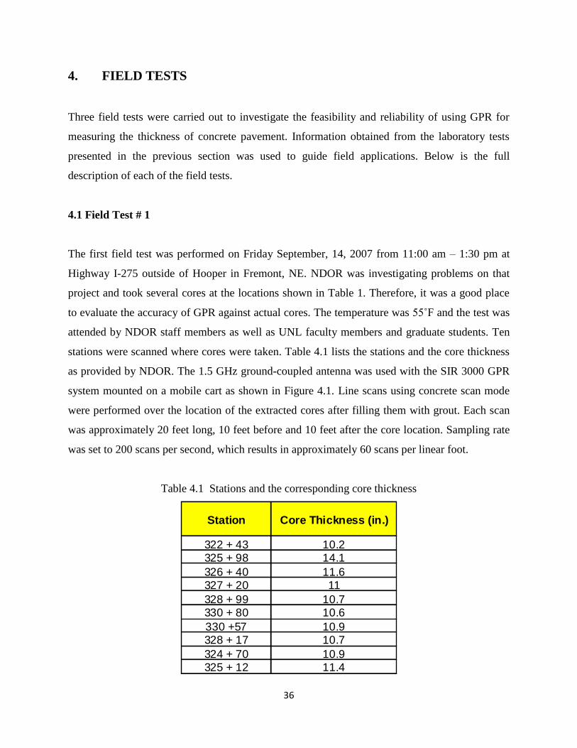
The first field test was performed on Friday September, 14, 2007 from 11:00 am – 1:30 pm at

Highway I-275 outside of Hooper in Fremont, NE. NDOR was investigating problems on that

project and took several cores at the locations shown in Table 1. Therefore, it was a good place

to evaluate the accuracy of GPR against actual cores. The temperature was 55˚F and the test was

attended by NDOR staff members as well as UNL faculty members and graduate students. Ten

stations were scanned where cores were taken. Table 4.1 lists the stations and the core thickness

as provided by NDOR. The 1.5 GHz ground-coupled antenna was used with the SIR 3000 GPR

system mounted on a mobile cart as shown in Figure 4.1. Line scans using concrete scan mode

were performed over the location of the extracted cores after filling them with grout. Each scan

was approximately 20 feet long, 10 feet before and 10 feet after the core location. Sampling rate

was set to 200 scans per second, which results in approximately 60 scans per linear foot.

Table 4.1 Stations and the corresponding core thickness

Station Core Thickness (in.)

322 + 43 10.2325 + 98 14.1

326 + 40 11.6327 + 20 11

328 + 99 10.7330 + 80 10.6

330 +57 10.9328 + 17 10.7

324 + 70 10.9325 + 12 11.4

37

Figure 4.1 GPR scan using SIR 3000 system on highway I-275

Figures 4.2, 4.3, and 4.4 show snapshots from the radargrams of scanning three different stations.

These figures also show the locations of the bottom surface of the concrete at these stations.

These radargrams indicate that GPR signal reflections at the bottom surface of the concrete are

weak and unclear, which make the surface detection difficult and thickness measurement

inaccurate. Based on thickness measurement obtained from the extracted cores, the RADAN

software was used to re-calculate the dielectric constant of the concrete. The dielectric value that

makes the depth of the bottom surface of the concrete obtained from GPR signal reflections

matches the actual pavement thickness was determined for each station. These values were found

to be substantially different from each other and some of them were slightly higher than the

standard range of conventional concrete (between 4 and 11). Therefore, it was concluded that it

is highly recommended to use metal objects at the interface between the concrete pavement and

its base layer. This will help producing strong reflections at the bottom surface of the concrete

that can be easily identified and used for more reliable thickness measurements.

38



Bottom of Concrete Reflection


39


Another scan was performed on the same day at the last station using a 2 ft x 2ft grid and the

SIR-20 GPR system. A paper grid was setup as shown in Figure 4.5 and several scanned at 4 in.

spacing. The bottom of the concrete was not detected due to a malfunction of the equipment at

that time.

Figure 4.5 Grid setup at station 325 + 12


40

4.2 Field Test # 2

The second field test was performed on Friday September, 21, 2007 from 11:00 am – 1:30 pm at

Highway 34 in Lincoln. The temperature was 85oF and the test was attended by NDOR staff

members as well as UNL faculty members and graduate students. In this test, two grid scans were

performed at two different locations where two 2 in. diameter metal rings (similar to the one used in lab

test #1) were put underneath 10 in. thick concrete pavement.

Scan # 1

A 2 ft x 2ft grid was made as shown in Figure 4.6 so that the center of the grid is the marked

location of the metal ring. The SIR 20 GPR system was used to scan the grid at 4 in. spacing.

Figure 4.7 and 4.8 show snapshots from the radargrams of the x-direction and y-direction scans

respectively. These figures demonstrate that the bottom surface of the concrete was clearly

detected at 10 in. deep as indicated by the signal reflections marked by the green lines. Also, the

metal ring underneath the concrete was detected, but less clearly, at the same depth as indicated

by the hyperbolas enclosed by the red circles. It should be noted that the metal ring was detected

at a different location from the marked one as shown in Figure 4.9. A concrete core was

extracted at the marked location (i.e. grid center), but the ring was not found. Another concrete

core was extracted later and the ring was found at the location detected by GPR.


41



42


Scan # 2

A 2 ft x 2ft grid was made as shown in Figure 4.10 so that the center of the grid is the marked

location of the metal ring. The SIR 20 GPR system was used to scan the grid at 2 in. spacing to

determine the location of the ring more accurately. Figure 4.11 and 4.12 show snapshots from the

radargrams of the x-direction and y-direction scans respectively. These figures demonstrate that

the bottom surface of the concrete was clearly detected at 10 in. deep as indicated by the signal

reflections marked by the green lines. Also, the metal ring underneath the concrete was detected,

but less clearly, at the same depth as indicated by the hyperbolas enclosed by the red circles. The

GPR found what was thought to be the washer, but the findings were inconclusive. NDOR

verified the location using a metal detector, cored that location, and found the metal ring at a

different location from the marked one as shown in Figure 4.13.

Based on the results of the two scans performed in the field test # 2, it was concluded that the

grid scan using SIR-20 GPR system is more accurate for measuring concrete pavement thickness

when metal objects are placed between the concrete and the base layer. It is recommended that

metal objects with larger surface than the 2 in. diameter rings be used to clearly and accurately

43

detected the bottom surface of the concrete. These recommendations have been considered in

field test # 3. It should be noted that in case of accidental movement of the metal object during

concrete pouring and/or vibration, several scans need to be taken to identify the object location,

which negatively affect the efficiency the technique.



44



45

4.3 Field Test # 3

The third field test was performed on Monday June, 30, 2008 between 8:30 am – 10:00 am at the

Fremont Bypass on Highway 30. Exact location is marked by a red rectangle on the map shown

in Figure 4.14. The temperature was 80oF and the test was attended by NDOR staff and UNL

faculty and graduate students. Eight GPR grid scans were performed at the 8 stations listed in

Table 4.2 where zinc steel clad plates were placed on the compacted base before paving. Figure

4.15 show the plate that is 11.8 in. diameter and ¼ in. thick. These plates were used to evaluate

the reliability of a relatively new non-destructive evaluation (NDE) technique, known by MIT

(Magnetic Imaging Technology) Scan-T2 system. This system for measuring the thickness of

concrete pavement is commercially available and was provided to NDOR by the Technology

Implementation Group (TIG) as a loan, which is supported by the Federal Highway

Administration. After curing, the location of each plate was marked on the concrete surface

based on MIT-Scan-T2 readings, which proven to be very accurate in all locations.

Figure 4.14 Location of the GPR scanned concrete pavement on Highway 30 in Fremont, NE

46

Table 4.2 Locations of plates scanned in field test #3

Pla te Sta tion

1 49+07

2 48+22

3 47+95

4 47+75

5 45+00

6 44+62

7 44+00

8 44+20

Figure 4.15 Steel plate placed underneath the concrete pavement

At each marked location, a 2 ft x 2 ft grid is placed and GPR grid scans were performed at 4”

spacing as shown in Figures 4.16. It should be noted that performing the eight grid scans took

about 40 minutes (i.e. 5 minutes per scan). In all the locations, the steel plate placed at the

interface between the bottom surface of concrete and the base layer was clearly detected as

indicated by the strong signal reflections at the plate location as shown in Figure 4.17.

Radargrams of all the 8 stations scanned in this field test are shown in Appendix B.

47

Figure 4.16 Grid scan at the marked location of the steel plate

Figure 4.17 Radargram of the GPR grid scan at one station in field test # 3

48

NDOR took cores at plate locations where the MIT-Scan T2 readings specified it on July 2,

2008. Actual concrete thickness of the two cores located at plates # 2 and # 7 were used to

calibrate the GPR scans (i.e calibration cores). The initial dielectic contant used in all the scans

was assumed to be 6.25 (i.e. Equipment default value for fairly dry concrete). The actual

dielectic contant of the concrete was calculated using the known thickness of calibration cores.

This value was found to be 7.23, which is higher than the initial value due to the early age of the

concrete and its higher moisture content. The difference between the initial and actual dielectric

constants of the concrete resulted in a correction factor for GPR thickness measurements of 0.93.

This correction factor was used to adjust GPR thickness measurements of the remaining six

plates. Table 4.3 lists the GPR initial thicknes meaurements, corrected thickness measurements,

and actual thickness measurement using 9-point readings of extracted cores (i.e verification

cores). The average of absolute differences in thickness measurement were found to be

approximetly ¼ in. (2.9 %) when all readings were considered. The average of absolute

differences in thickness measurement were found to be approximetly 1/8 in. (1.4 %) when the

reading # 4 is eliminated. This is because the error in reading # 4 was found to be unreasonablly

high. Same conclusion was confirmed for the same reading using MIT Scan-T2 system.


Plate StationGPR-measured

thickness (in)

Corrected GPR-

measured

thickness (in)

Actual

Thickness (in)

Difference between

Actual and GPR-

measured thickness(in)

Difference between

Actual and GPR-

measured thickness(%)

1 49+07 10.7 9.96 9.70 0.26 2.7%

2 48+22 * 11.3 10.52 10.49 0.03 0.3%

3 47+95 11.6 10.80 10.67 0.13 1.2%

4 47+75 10.2 9.50 8.64 0.86 9.9%

5 45+00 9.0 8.38 8.44 0.06 0.7%

6 44+62 9.3 8.66 8.75 0.09 1.0%

7 44+00 * 8.9 8.29 8.31 0.02 0.3%

8 44+20 10.1 9.40 9.26 0.14 1.5%

Correction Factor 0.93 2/8 2.9%

* Calibration Station 1/8 1.4%

Average All

Average without #4

49

4.4 Field Test # 4

The forth field test was performed on Hwy 2 in Lincoln, NE (location is marked by a red

rectangle on the map shown in Figure 4.18). The test was performed on two days Thursday June

18, 2009 and Friday June 26, 2009 due to some technical problems with the GPR equipment on

the first day. The two tests were attended by NDOR staff and UNL faculty and graduate students.

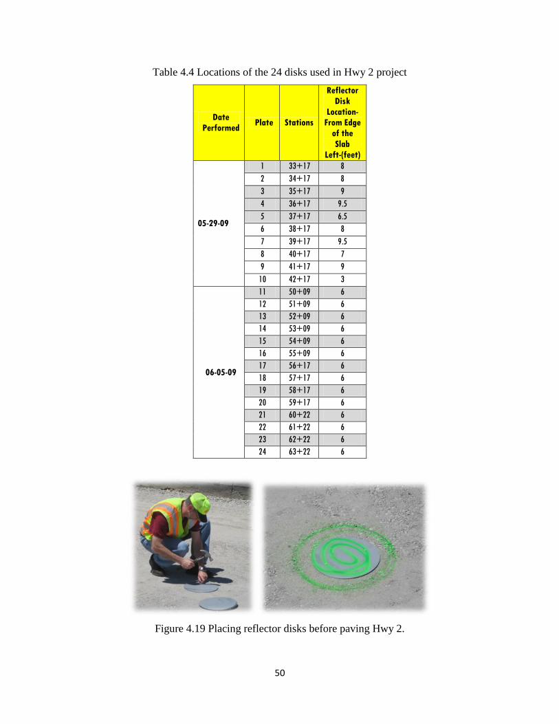
Table 4.4 lists the location of 24 zinc steel clad disks placed on the compacted base before

paving to be used as reflectors for thickness measurement using GPR and MIT techniques. Only

the shaded stations in Table 4.4 were scanned using GPR. The first four scans were performed

on June 18, 2009 (test a), while the seven remaining scans were performed on June 26, 2009 (test

b). Figure 4.19 shows pictures of placing and anchoring one of the disks on the road before

paving by NDOR personnel.

Figure 4.18 Location of the GPR scanned concrete pavement on Hwy 2, Lincoln, NE

50

Table 4.4 Locations of the 24 disks used in Hwy 2 project

Date

Performed Plate Stations

Reflector

Disk

Location-

From Edge

of the

Slab

Left-(feet)

05-29-09

1 33+17 8

2 34+17 8

3 35+17 9

4 36+17 9.5

5 37+17 6.5

6 38+17 8

7 39+17 9.5

8 40+17 7

9 41+17 9

10 42+17 3

06-05-09

11 50+09 6

12 51+09 6

13 52+09 6

14 53+09 6

15 54+09 6

16 55+09 6

17 56+17 6

18 57+17 6

19 58+17 6

20 59+17 6

21 60+22 6

22 61+22 6

23 62+22 6

24 63+22 6

Figure 4.19 Placing reflector disks before paving Hwy 2.

51


spacing as shown in Figures 4.20. In all the locations, the steel plate placed at the interface

between the bottom surface of concrete and the base layer was clearly detected as indicated by

the strong signal reflections at the plate location as shown in Figure 4.21.



52

NDOR took cores at all reflector disk locations as specified by the MIT-scan readings. Actual

concrete thickness of the two cores located at plates # 3 and # 15 were used to calibrate the GPR

scans (i.e calibration cores). The initial dielectic contant used in all the scans was assumed to be

6.25 (i.e. Equipment default value for fairly dry concrete). The actual dielectic contant of the

concrete was calculated using the known thickness of calibration cores and was found to be 6.64

and 6.93 for the two tests, which is higher than the initial value due to the early age of the

concrete and its higher moisture content. The difference between the initial and actual dielectric

constants of the concrete resulted in correction factors for GPR thickness measurements of 0.97

and 0.95 respectively. These correction factors were used to adjust GPR thickness measurements

at the remaining locations. Tables 4.5 and 4.6 list the GPR initial meaurement, corrected

measurements, and the actual thickness measured from extracted cores for the two tests. The

average of absolute differences in thickness measurement were found to be approximetly 0.11

and 0.03 in, which corresponds to 1.2% and 0.4 % for tests a and b respectively.

Table 4.5 Results of field test #4a


thickness (in)

Corrected GPR-

measured

thickness (in)

Actual

Thickness (in)

Difference between

Actual and GPR-


Difference between

Actual and GPR-


1 33+17 9 3/4 9.44 9.37 0.07 0.7%

3 35+17 * 9 1/2 9.20 9.20 0.00 0.0%

5 37+17 9 3/8 9.08 9.22 0.14 1.5%

4 36+17 9 1/4 8.96 9.18 0.23 2.5%

9 1/2 9.24 0.11 1.2%

0.97

Average

Correction Factor Table 4.6 Results of field test #4b


thickness (in)

Corrected GPR-

measured

thickness (in)

Actual

Thickness (in)

Difference between

Actual and GPR-


Difference between

Actual and GPR-


11 50+09 9 3/4 9.26 9.33 0.07 0.70%

13 52+09 9 7/8 9.38 9.31 0.08 0.81%

15 54+09 * 10 9.50 9.50 0.00 0.00%

17 56+17 10 9.50 9.50 0.00 0.00%

19 58+17 10 1/8 9.62 9.61 0.01 0.13%

21 60+22 10 9.50 9.46 0.04 0.41%

23 62+22 9 3/4 9.26 9.22 0.04 0.44%

10 9.43 9.42 0.03 0.36%

0.95

* Calibration Station

Correction Factor

Average

53

4.5 Field Test # 5

The fifth field test was performed at the I-80 west of 56th

street in Lincoln, NE (location is

marked by a red rectangle on the map shown in Figure 4.22). The test was performed on Friday

August 28, 2009 and was attended by NDOR staff and UNL faculty and graduate students. Table

4.7 lists the location of 22 zinc steel clad disks placed on the compacted base before paving to be

used as reflectors for thickness measurement using GPR and MIT techniques. Only the shaded

stations in Table 4.7 were scanned using GPR. Figure 4.23 shows pictures of placing and

anchoring one of the disks on the road before paving by NDOR personnel.

Figure 4.22 Location of the GPR scanned concrete pavement on I-80, Lincoln, NE

54

Table 4.7 Locations of the 22 disks used in I-80 project

Figure 4.23 Placing reflector disk before paving I-80.

Date

Performed Plate Stations

Reflector

Disk

Location-

Westbound

Feet Lt

07-23-09

1 927+00 10

2 923+00 8

3 925+03 8

4 924+03 8

5 924+03 8

6 923+05 8

7 922+02 8

8 921+00 8

9 920+00 8

10 919+00 8

11 918+00 8

07-24-09

12 917+00 8

13 916+00 8

14 915+00 8

15 914+00 8

16 913+00 8

17 912+00 8

18 911+00 8

19 910+00 8

20 910+03 8

21 909+00 8

22 908+00 8

55


spacing as shown in Figures 4.24. In all the locations, the steel plate placed at the interface

between the bottom surface of concrete and the base layer was clearly detected as indicated by

the strong signal reflections at the plate location as shown in Figure 4.25.



56

NDOR took cores at all reflector disk locations as specified by MIT-scan readings. Actual

concrete thickness of the two cores located at plate # 12 was used to calibrate the GPR scans (i.e

calibration core). The initial dielectic contant used in all the scans was assumed to be 6.25 (i.e.

Equipment default value for fairly dry concrete). The actual dielectic contant of the concrete was

calculated using the known thickness of calibration cores and was found to be 7.07, which is

higher than the initial value due to the early age of the concrete and its higher moisture content.

The difference between the initial and actual dielectric constants of the concrete resulted in a

correction factor for GPR thickness measurements of 0.94. This correction factor was used to

adjust GPR thickness measurements at the remaining locations. Tables 4.8 lists the GPR initial

meaurement, corrected measurements, and the actual thickness measured from extracted cores.

The average of absolute difference in thickness measurement was found to be approximetly 0.1

in., which corresponds to 0.75%



thickness (in)

Corrected GPR-

measured

thickness (in)

Actual

Thickness (in)

Difference between

Actual and GPR-


Difference between

Actual and GPR-


2 9+26 13 1/2 12.68 12.94 0.26 2.03%

4 9+24 13 3/4 12.91 12.89 0.02 0.18%

6 9+22 13 5/8 12.80 12.92 0.12 0.97%

8 9+20 13 7/8 13.03 12.96 0.07 0.54%

10 9+18 13 5/8 12.80 12.99 0.19 1.50%

12 9+16 * 13 7/8 13.03 13.03 0.00 0.00%

14 9+14 14 13.15 13.24 0.09 0.70%

16 9+12 13 5/8 12.80 12.89 0.09 0.74%

18 9+10 14 13.15 13.07 0.08 0.59%

20 9+8 13 7/8 13.03 12.99 0.04 0.31%

13 7/9 12.94 12.99 0.10 0.75%

0.94

* Calibration Station

Correction Factor

Average

57

5. BENEFIT- COST ANALYSIS

Table 5.1 presents a comparison between the proposed GPR pavement quality assurance

technique and the traditional coring technique in terms of cost (initial cost and operating cost)

and benefits (accuracy, time and destructiveness). This comparison is based on 1 mile

assessment using 8 cores for the traditional method and 8 scans + 2 calibration cores for GPR

method. The operating cost was calculated assuming a labor hourly rate of $50, cost of metal

plate of $8.75, and cost of core drilling and filling material as $2.5. Time was calculated

assuming 10 mins for core extraction, 5 mins for core thickness measurement using 9 point

reading, 5 mins for one GPR scan, and 10 mins for GPR scan analysis. These estimates were

based on the investigators’ experience in this project and information provided by NDOR

personnel.

Table 5.1. Benefit-Cost Comparison Between GPR and Coring

Criteria GPR (8 scans + 2 cores) Coring (8 cores)

Destructiveness Nondestructive Destructive

Accuracy 98.50% 100%

Time 8 x (5 + 10) + 2 x (10 + 5) = 2.5 hrs 8 x (10 + 5) = 2 hrs

Initial Cost $35,000 0

Operating Cost $200 $120

Based on this table, it can be concluded that the major advantage of using GPR in

concrete pavement thickness measurement is the significant reduction in the number of drilled

cores, which is a destructive technique that affect the pavement durability, while providing a

comparable accuracy. The proposed methodology provided an accuracy as high as 98.5% (1/8 of

inch), which is better than the values presented in the literature. Although GPR equipment has

higher initial and operating cost than core drilling, the minimization of core drilling might result

in lower pavement maintenance cost in the long term. It should be noted that, as any new

technique, attention must be paid to proper training for GPR to provide reliable and consistent

results in a cost-effective fashion. Also, the lack of specifications is an important limitation and

needs to be addressed.

58

6. SUMMARY AND CONCLUSIONS

In this project, the feasibility of the use of Ground Penetrating Radar (GPR) as a non-

destructive evaluation technique for measuring the thickness of concrete pavement was

investigated. Currently, NDOR perform thickness measurement of concrete pavement according

to ASTM C174. Although this method provides an accurate thickness measurement, it is

destructive, labor intensive, and time consuming. Moreover, concrete cores are usually extracted

every 750 ft, which provides inadequate information about the thickness profile of pavement

sections. The GPR technique was proposed because of its advantages over drilled core, such as

being non-destructive, user friendly, efficient, and cost-effective when applied to long pavement

sections. However, the literature of using GPR for measuring the thickness of concrete pavement

does not provide sufficient evidence on its accuracy and consistency. Therefore, the objective of

this project was to investigate its accuracy relative to drilled cores in measuring thickness of

concrete pavement for quality assurance purposes. The GPR systems GSSI SIR20 and GSSI

SIR3000 with a high resolution 1.6 MHz ground coupled antenna were used. Three laboratory

tests and three field tests were performed within this project. Different metal objects were used

underneath the concrete to improve GPR signal reflectivity at the bottom surface of the concrete

pavement. Also, GPR scans were performed at different concrete ages to estimate the variation in

the dielectric constant of the concrete.

Based on the results of the lab and field tests, the following conclusions were made:

1- GPR is an efficient technique for measuring the thickness of concrete pavement. Grid scans

can be performed in as short as 5 minutes per location, while data analysis can be as low as

10 minutes per scan.

2- GPR signal reflections at the interface between the bottom of the concrete layer and the base

layer are neither clear nor reliable due to the proximity of the dielectric constant of the

concrete and that of the base layer.

3- GPR signal reflections at the interface between the bottom of the concrete layer and the base

layer are clear and reliable when metal objects are placed on the top of the base layer before

paving. Although GPR can accurately locate these objects, it is recommended for rapid

evaluation that the objects be anchored properly so they do not shift while pouring and/or

vibrating the concrete.

59

4- The surface area of the metal object used is more important than its thickness for being easily

and clearly detected by GPR. Flat objects, such as plates, with rectangularity ratio close to 1,

are more efficient than narrow and long objects, such as rods or strips.

5- The dielectric of the concrete is highly dependent on the concrete age, which significantly

affects the measured thickness. The lab test results indicated that using a constant value of

the concrete dielectric results in a significant reduction in the measured thickness of 0.01 in

per day as the concrete gets older. That is why calibration cores are needed.

6- Calibration cores are necessary for correcting the assumed value of dielectric constant of

concrete. Based on the field test results, one or two drilled cores are satisfactory for

calibrating ten readings.

7- The average difference in concrete thickness measurements using GPR (with calibration

cores) and drilled cores is found to be 1/8 in. for 10 - 13 in. thick pavement. This represents

an average measurement accuracy of 98.5%, which is relatively high. It should be noted that

the accuracy of GPR measurements is highly dependent on the calibration process, which

requires the extraction of limited number of cores.

60

7. IMPLEMENTATION PLAN

One of the objectives of this research was to evaluate the feasibility of using Ground

Penetrating Radar for measuring pavement thickness. While this research was taking place,

NDOR’s In-House Research was also evaluating other products for measuring pavement depth.

As a result of these evaluations, some of the conclusions drawn from this study have put into

question how effective the GPR compares with other products for measuring pavement depth.

NDOR has found other equipment requires no calibration, saves time with less data input, its

ease of use and low cost. NDOR is still evaluating other products that are in the market today;

therefore, the Department will not implement the GPR equipment at this time.

Wally Heyen

NDOR Portland Cement Concrete Engineer

61

8. REFERENCES

Al-Qadi, I. L., and Lahour, S. (2004) “Ground Penetrating Radar: State of the Practice for

Pavement Assessment”, Journal of Materials Evaluation, Vol. 42, No. 7, pp. 759-763.

ASTM (2006a) “Standard Test Method for Determining the Thickness of Bound Pavement

Layers Using Short-Pulse Radar”, American Society for Testing and Materials D4748-06

ASTM (2006b) “Standard Test Method for Measuring Thickness of Concrete Elements Using

Drilled Concrete Cores”, American Society for Testing and Materials C174/C174M-06

FHWA, Federal Highway Administration (2004) “Priority, Market-Ready Technologies and

Innovations: Ground-Penetrating Radar”, US Department of Transportation.

Kurtz, James; Choubane, Bouzid; Fernando, Emannuel. “Improved Roadway Subsurface

Thickness Measurement and Anomaly Identification with Ground Penetrating Radar.”

Florida Department of Transportation: Summary of Final Report. June 2001.

Loulizi, A., Al-Qadi, I. L., and Lahouar, S. (2003) “Optimization of Ground-Penetrating Radar

Data to Predict Layer Thickness in Flexible Pavements”, ASCE Journal of Transportation

Engineering, Vol. 129, No. 1, pp. 93-99.

Maierhofer, C. (2003) “Nondestructive Evaluation of Concrete Infrastructure with Ground

Penetrating Radar”, ASCE Journal of Materials in Civil Engineering, Vol. 15, No. 3, pp. 287-

297.

Maser, K. R (1996) “Condition Assessment of Transportation Infrastructure Using Ground-

Penetrating Radar”, ASCE Journal of Infrastructure Systems, Vol. 2, No. 2, pp. 94-101

Olhoeft, Gary; Smith, Stanley. “Automatic Processing and Modeling of GPR Data for Pavement

Thickness and Properties.” Procedings of the 8th

International Conference on Ground

Penetrating Radar. Gold Coast, Australia. 23 May 2000.

Willett, D. A., Mahboub, K. C., and Rister, B. (2006) “Accuracy of Ground-Penetrating Radar

for Pavement-Layer Thickness Analysis”, ASCE Journal of Transportation Engineering, Vol.

132, No. 1, pp. 96-103

62

APPENDIX A

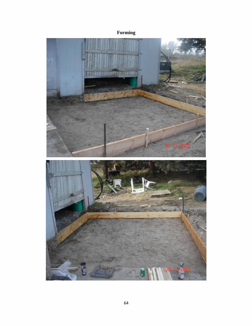
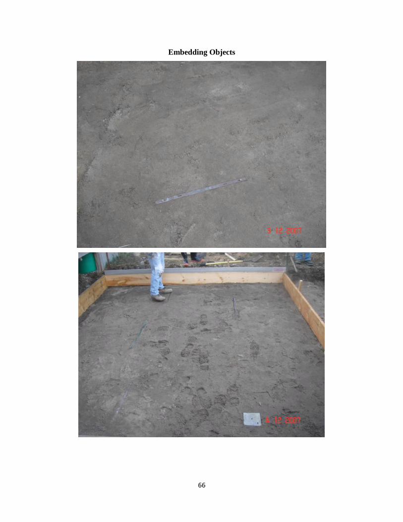
Construction Photos of the Test Driveway

63

Leveling

64

Forming

65

Compacting Subgrade

66

Embedding Objects

67

Pouring Concrete

68

Vibrating and Finishing

69

Covering of Concrete

70

Coring

use of ground penetrating radar for construction quality ... · 3 1. report no. p307 2. government...

Documents