Use of Piezoelectric Techniques Monitoring Continuum Damage Of

Structures

By

Sikhulile Khululeka Nhassengo

Submitted in partial fulfilment of the requirements for the degree of Master of Technology degree in Mechanical Engineering in the Faculty of Engineering and Built

Environment at the Durban University of Technology

Supervisor: Prof. P. Tabakov

Co supervisor: Prof. K. Duffy

August 2009

1

TABLE OF CONTENTS ABSTRACT 3 ACKNOWLEDGEMENTS 4 NOTATION 5 LIST OF FIGURES 7 LIST OF TABLES 9 1. INTRODUCTION 10-15 1.1 Research Overview 10 1.2 Research Hypothesis 12 1.3 Research Objective 13 1.4 Research Layout 14 2. LITERATURE REVIEW 16-35 Introduction 16 2.1 Material 17 2.1.1 Ductile Steel 19 2.1.2 Processing Techniques 19 2.2 Low Cycle Fatigue

2.2.1 Introduction 21 2.3 Piezoelectric

2.3.1 Introduction 25 2.3.2 Operational Principles 31 2.3.3 Electrical Properties 32 2.3.4 Sensor Design 33

Conclusion 34 3. UNI-AXIAL LOADING 36-47 Introduction 37 3.1 Tensile Testing Machine 37 3.1.1 Screw Driven Testing 37 3.1.2 Servo-hydraulic Testing 39 3.2 Experimental Methods 3.2.1 Materials 40 3.2.2 Specimen preparation for Micro-structure 40 3.2.2.1 Specimen Mounting 41

2

3.2.2.2 Specimen preparation 42 3.2.3 Test Specimen Preparation 43 3.2.4 Testing Condition 44 3.3 Quasi-Static Mechanical Test 3.3.1 Tensile Test/ Compression Tests 45 3.3.2 Optical Microscope 46 Conclusion 47 4. EXPERIMENTAL METHODS (DYNAMIC) 48-58 Introduction 48 4.1 Fatigue Bending Machine 4.1.1 Cantilever Beam Machine 49 4.1.2 Rotating Beam Machine 50 4.2 Experimental Methods 4.2.1 Materials 51 4.2.2 Strain Measuring Equipment 4.2.2.1 Strain Gauge 51 4.2.2.2 Piezoelectric Sensor 53 4.2.3 Strain Acquisition System 54 4.2.4 Testing Condition 55 4.3 Dynamic Mechanical Test 4.3.1 Elasto-Plastic Fatigue Test 56 4.3.2 Piezo-Elastic Fatigue Test 57

Conclusion 58

5. TECHNICAL BACKGROUND 59-72 Introduction 59 5.1 Elasticity 60 5.2 Plasticity 61 5.3 Elastic Damage 65 5.4 Fatigue Damage 66 5.5 Elastic coupled with damage 67 5.6 Plastic coupled with damage 69

Conclusion 71 6. RESULTS AND DISCUSSION 73-92

Introduction 73 6.1 Uni-axial Loading 74 6.2 Cyclic Loading 80 Conclusion 91

7. CONCLUSION 93-95 8. BIBLIOGRAPHY 96-104

3

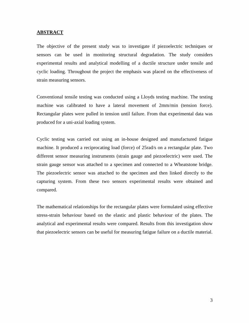
ABSTRACT

The objective of the present study was to investigate if piezoelectric techniques or

sensors can be used in monitoring structural degradation. The study considers

experimental results and analytical modelling of a ductile structure under tensile and

cyclic loading. Throughout the project the emphasis was placed on the effectiveness of

strain measuring sensors.

Conventional tensile testing was conducted using a Lloyds testing machine. The testing

machine was calibrated to have a lateral movement of 2mm/min (tension force).

Rectangular plates were pulled in tension until failure. From that experimental data was

produced for a uni-axial loading system.

Cyclic testing was carried out using an in-house designed and manufactured fatigue

machine. It produced a reciprocating load (force) of 25rad/s on a rectangular plate. Two

different sensor measuring instruments (strain gauge and piezoelectric) were used. The

strain gauge sensor was attached to a specimen and connected to a Wheatstone bridge.

The piezoelectric sensor was attached to the specimen and then linked directly to the

capturing system. From these two sensors experimental results were obtained and

compared.

The mathematical relationships for the rectangular plates were formulated using effective

stress-strain behaviour based on the elastic and plastic behaviour of the plates. The

analytical and experimental results were compared. Results from this investigation show

that piezoelectric sensors can be useful for measuring fatigue failure on a ductile material.

4

Acknowledgements

A special thank you to my supervisor Prof Pavel Tabakov, co-supervisor Prof Kevin

Duffy for their support and guidance throughout this research project. Justice would not

be served if I do not thank all the staff members in the department of Mechanical

Engineering at the Durban University of Technology. Without their support this would

not have been possible.

I also want to extend my appreciation to my family (Nhassengo- Laice) and Temantfulini

Mamba for the support and constant loving they have shown during my journey of

discovery as a researcher.

5

NOTATION

D Damage

cD Critical Damage

uD Ductility

E Modulus of Elasticity

G Modulus of Rigidity

h Hardening Modulus

I Moment of Inertia

321 ,, JJJ Invariant of the stress deviator

K Elastic Bulk Modulus

nml ,, Direction cosines of normal to a plane

N Number of cycles

FN Number of cycles to failure due to pure bending

p Accumulated plastic strain

r Heat production per unit volume

R Isotropic hardening variable

*s Second polar stress tensor

W Strain energy

Y Elastic energy density release rate

α Kinematic hardening variable

γ Shear strain

ijδ Kronecker delta

6

ijε Total Strain

eijε Elastic strain tensor

pijε Plastic strain tensor

Dε Damage threshold strain

λ Lame’s constant of elasticity

υ Poisson’s ratio

ijσ Stress tensor

321 ,, σσσ Principal stress

mσ Mean stress

ijσ ′ Deviatoric stress tensor

yσ Yield stress

eqσ Von Mises equivalent stress

τ Shear stress

Dϕ Damage Dissipation potential

*ϕ Dual potential

Φ Specific power of dissipation

7

LIST OF FIGURES

Figure 1.0 Block diagram of a Smart Structure

Figure 1.1 Schematic symbol and electronic model of a piezoelectric sensor

Figure 1.2 Frequency response of a piezoelectric sensor

Figure 1.3 Metal disks with piezo-material, used in buzzers or as contact

microphones

Figure 3.1 (a) The Screw-Driven Testing Machine, (b) Servohydraulic Testing

Machine

Figure 3.2 Show a specimen mounted using cold mounting

Figure 3.3 Grinding wheel used for polishing cold mounted specimens

Figure 3.4 The Llyods uniaxial testing machine with an extensometer

Figure 3.5 Microscope with the magnification of 800 X lens

Figure 4.1 Cantilever Beam Machine

Figure 4.2 R.R. Moore Rotating Beam Machine

Figure 4.3 Illustrates the conditioning of the signal using Lab-View

Figure 4.4 Show the serrated plates used for clamping the specimen

Figure 4.5 Block Diagram for Data Acquisition

Figure 4.6 Fatigue Bending Machine with reciprocating motion Figure 6.1 Three samples of DOCOL 800 DP steel

Figure 6.2 Load displacement curves for a rectangular specimen for a fixed beam

subjected to a uniformly distributed load (1SE)

8

Figure 6.3 Analysis of DOCOL 800 DP tensile test experiment for a rectangular

specimen using the analytical method (1SE)

Figure 6.4 Evolution of damage for DOCOL 800 DP (1SE)

Figure 6.5 Experimental record of cyclic pure bending curve using strain gauge

sensors

Figure 6.6 Cyclic loading for pure bending curve using piezoelectric sensor

Figure 6.7 Tensile behaviour of the rectangual specimen under different strains

using strain gauges

Figure 6.8 Tensile behaviour of the cyclic curve for a strain gauge sensor

Figure 6.9 Tensile behaviour of the rectangular specimen under different strain

using pieszoelectric sesors (1SE)

Figure 6.10 Tensile curve of the cyclic curve using piezoelectric sensors per cycle

(1SE)

Figure 6.11 Comparison between experimental data and the analytical data of

DOCOL 800 DP steel using a strain gauge sensor (1SE)

Figure 6.12 Relationship between the analytical results and the experimental data of

strain gauge sensor compared to the experimental curve of the piezoelectric sensor

(1SE)

Figure 6.13 Adjusted analytical curve for the piezoelectric sensor against the

experimental curve for the strain gauge (1SE)

Figure 6.14 The adjusted analytical curves for the piezoelectric sensor is compared

with the analytical results for the strain gauge sensor (1SE)

9

LIST OF TABLES

Table 1: Analysis of the Docol 800 DP tension specimen: average chemical

composition

Table 2: States the initial conditions which were experienced during testing

Table 3: Characteristic data and dimension of the strain gauge are displayed in the

following

Table 4: Characteristics of a Quick-Mount bending performance actuator

10

Chapter 1

INTRODUCTION

1. RESEARCH OVERVIEW

Considerable effort has been devoted in recent years to the study of the behaviour of

structures when subjected to cyclic loading conditions. Cyclic loading in most machines,

structures and dynamic systems is undesirable because it leads to fatigue failure. It has

been reported that nearly 90% of machinery, structures and dynamic systems which

experience cyclic loading fail due to fatigue [25, 46]. This type of failure occurs suddenly

without any warning causing problems for industries due to it being difficult to avoid [25,

46]. It is therefore important to know how much degradation has taken place at any

particular time in order to monitor the conditions of the structure and avoid catastrophic

failure from occurring. Successful assessment of a component’s life places a great

demand in understanding the material behaviour under different strain histories involving

cyclic plasticity.

11

Ductile materials undergo large plastic deformations before rupture. The accumulated

plastic strains are associated with material degradation due to thermodynamic

microstructural changes like nucleation, growth and coalescence of micro-voids [8].

Low-cycle fatigue testing is carried out under total strain controlled limits. The plastic

strain component is determined retrospectively after testing by considering the hysteresis

loop closest to the mid-life [35].

In a strain controlled low-cycle fatigue test it is customary to use a contacting

extensometer. However, the extensometer can cause premature fractures at the contact

points by inducing localized plastic deformation, particularly in a soft metal such as a

lead–tin solder [34]. To avoid this problem, a non-contacting, digital-image measurement

system has been developed to measure the displacement of the specimen gauge length

during cyclic loading [34].

All controlled low-cycle fatigue tests recognize that the rate of controlled time-dependent

damage process is influence by the cyclic deformation and fracture behaviour of alloys

[69].

Chan and Li [7] developed a method of assessing fatigue damage of a Tsing Ma Bridge

(TBM). This led to fatigue damage analysis and service life prediction of the TMB using

the strain time history data by the structural health monitoring system of the bridge [7]. In

2002, a close relationship was found to exist between the concentration of linear defects

and the stability of the resonant frequency as a function of temperature and time [57].

12

Due to the importance and necessity of the problem and limited research history

available, an in-depth study on the monitoring of degradation of machine components

using the smart material sensors known as piezoelectric is required. Therefore, the

purpose of this study is to see if piezoelectric sensors can be used to measure fatigue

failure in ductile metals.

1.2 RESEARCH HYPOTHESIS

The automotive industry is continuously faced with a huge task of increasing productivity

using their aging machines while reducing their operational costs of processing. This

means unexpected or sudden shut downs are non-negotiable during operation. This

exercise can cause companies millions of Rand in revenue due to their maintenance bill.

Therefore, it is important to find systems which could be used in self-monitoring of

structures.

The intended outcome of this research work is to see if health structures can be produced

to reduce unexpected catastrophic failure of structures. This means techniques will be

tested to see if they can be used to measure and track the progress of fatigue failure in

structures. These techniques will integrate experimental behaviour of the structure

together with theoretical damage knowledge of structures. The theoretical background

information involves the elasto-plastic behaviour of the material under the loading

condition.

13

Being able to predict the remaining life of the health structure plays an important role in

determining the exact failure period. This type of information becomes handy when

scheduling maintenance work. It also means that the maximum usage of the machine can

also be utilized, so increasing productivity.

Solving this problem can be done by firstly having numerous experimental tests carried

out on rectangular specimens. These tests will produce important data relating to the

material properties. Secondly, calculating and producing damage models using

continuum mechanics theory. Thirdly, merging the two sets of information (experiments

together with analytical analysis) and determining whether the margin of error is

acceptable.

If the procedures followed are correct then it should be possible to see if piezoelectric

techniques can be used to track the degradation process of structures.

1.3 RESEARCH OBJECTIVE

The primary objective of this thesis is to experimentally investigate if piezoelectric

materials can be used in monitoring structural degradation caused by low-cycle fatigue.

An analytical development of fatigue failure using continuum damage mechanics will

also be conducted. This will link the experimental relationship with damage mechanics

models. The aim behind such work is the need to manufacture smart structures which are

14

capable of self-monitoring. This will cause a reduction in abrupt failure of components

under high cyclic straining or stressing, like in turbine blades.

In the first stage, the metal specimen or component will be uni-axially loaded until failure

occurs. This experimental study will provide the mechanical behaviour of the ductile

steel specimen during conventional tensile tests. This standard engineering procedure will

be useful in characterizing the relationship between elastic and plastic components

relating to the mechanical behaviour of materials. In the elastic and plastic region, both

elastic and plastic strain components will be analyzed using the Prandtl and Reuss

method [16]. When the analysis on the static failure is completed then fatigue testing will

be initiated.

This part of the investigation shows a cantilever plate with a piezoelectric material as a

sensor being cyclically loaded using a fatigue bending machine. The piezoelectric sensor

network will be integrated into the structure to monitor the material condition throughout

its lifeline. Therefore, the sensors will be permanently bonded to the specimen by means

of adhesive. The adhesive interface provides the necessary mechanical coupling needed

to transfer the force and strain between the piezoelectric element and the specimen [60].

A damage growth model for low-cycle fatigue damage will be developed using a

continuum damage mechanics approach.

15

1.4 RESEARCH LAYOUT

The outline of the thesis is as follows: the introduction to this study is presented in

Chapter 1.

Chapter 2 looks at the theoretical knowledge behind low cycle fatigue and strain

measurement.

Chapter 3 and 4 involves the Tensile Test, and the Cyclic Test. It first focuses on the

experimental and numerical study of the mechanical behaviour of DOCOL 800 DP steel

specimen during conventional tensile tests. This standard engineering procedure is useful

in characterizing some relevant elastic and plastic variables relating to the mechanical

behaviour of materials. Then an analysis on structural degradation of the Ductile steel

specimen under fatigue bending testing will be conducted.

In Chapter 5; continuum mechanics models will be used to develop thresholds for

elasto-plastic behaviour. By placing suitable thresholds, it is possible to detect from the

onset the final stage of damage in the structure before failure occurs. The basis for

modelling damage mechanics of the ductile material is presented. The use of standard

derivations of elasto-plastic-damage models are formulated from the above approach.

The numerical results obtained will be to study the effect of damage growth on structural

materials.

The numerical results are presented in Chapter 6 and conclusion in Chapter 7.

16

Chapter 2

LITERATURE REVIEW

This chapter deals with the relevant literature regarding the pertinent issue under

investigation in the study.

Material processing techniques are also presented. These preparation techniques allows

for the easy shaping of the specimen either by cold rolling or hot rolling into a

rectangular cross-section.

Low cycle fatigue and piezoelectric materials are discussed in their elementary stage. As

such, significant articles and studies are explored in relation to these sections. The

theoretical framework is presented as applied to this study.

17

2.1 MATERIAL

With technology improving, and the industrial revolution, the process of manufacturing

steel in large amounts was needed. This called for the iron mining industry to begin with

John Winthrop Jr. by establishing an iron work on the Saugus River in Lynn,

Massachusetts [27].

In 1750, the British passed the Iron Act, one of the first of the Trade and Navigation Acts

that were to be a major cause of the industrial revolution. The act forbade the building of

mills in the colonies’ but later American pig iron was admitted into Britain duty-free

[32]. More than five thousand tons were shipped abroad from Virginia, Maryland,

Pennsylvania and New York. When the War ended, the manufacture of iron products

increased dramatically which led to the era of the exploration of steam.

In 1856 the British engineer Sir Henry Bessemer developed the Bessemer process for

making steel [27, 32]. Two years later the Siemens-Martin open hearth method was also

developed for processing steel. Once perfected, these processes greatly lowered the cost

of steel production and allowed the increasingly lavish use of steel for railroads,

construction, and other industrial purposes. The first Bessemer converter in the United

States was made operational in 1864 and four years later Abram S. Hewitt built the first

open hearth furnace [27, 32].

18

1901 helped shape the modern industry by their visionary thinking and their business

ethics [27]. With American steel production peaking in 1969, it prompted new, vibrant

and more efficient steel plants with much lower labour cost to be built outside the United

States of America.

The methods of making steel have not changed dramatically over the past 30 years; but

the mechanical properties of steel have been improved [32]. With continued need for high

strength steels at low cost, the carbon ratio has been adjusted. The demand for high

quality has seen an increase in alloying and processing of metals.

A metal alloy is usually melted together with two or more chemical elements where the

bulk of the material consists of one or more metals. This has produced a wide range of

metallic and non metallic chemical elements used in alloying the principal engineering

metal. Some commonly used elements are boron, carbon, magnesium, silicon etc (see

Table 1). The amounts and combinations of alloying element used with various metals

have major effects on their strength, ductility, temperature resistance, corrosion

resistance, and other properties [17].

The metal alloy has pushed back the boundaries of strength, weight saving and

environmental benefits. The high yield strength of the steel enables reduction of the

thickness of the steel (or product) resulting in low material costs. If DOCOL UHS steel is

used for reducing weight in a motor vehicle, the energy consumption and exhaust

emission are reduced [17].

19

2.1.1 DUCTILE STEEL - DOCOL 800DP

The cold reduced ultra high strength steel from SSAB Tunnplat-designated DOCOL

UHS- have guaranteed minimum tensile strengths ranging between 800 and 1400 N/mm2

and yield strengths in excess of 550N/mm2. DOCOL UHS steel offers many competitive

benefits [17].

The high strength of DOCOL UHS steel offers opportunities for vast weight saving

which, in turn, offers great environmental benefits which stem from the energy savings

and the reduction of emissions at plants or factories due to the strength of the material

being used since there is no heat treatment furnace [17].

A thinner material also enables engineers to develop entirely new designs that would

have been impossible in the past [17]. The cold reduced ultra high strength steel-

designated DOCOL UHS- acquire their unique properties in the SSAB Tunnplat

continuous annealing line.

2.1.2 PROCESSING TECHNIQUES

The steels are annealed at temperatures between 750-850oC, depending on the grade of

steel and then hardened by quenching in water [17]. The next stage is the tempering

process which is carried out at a temperature between 200-400oC, when it acquires its

20

final structure to which the steel owes its toughness and good formability. Both the

annealing and tempering process are carried out at atmospheric conditions to prevent the

steel from oxidizing. Also, the steel runs through a pickling bath between quenching and

tempering in order to remove the thin oxide film formed in the quenching process [17].

The micro-structure of the steel consists of martensite which is a hard phase and the

ferrite which is soft. The strength of the steel is carefully increased with an increase in the

content of the hard martensite phase. The proportion of martensite is determined by the

carbon content of the steel and the temperature cycle to which the steel is subjected in the

continuous annealing process [17].

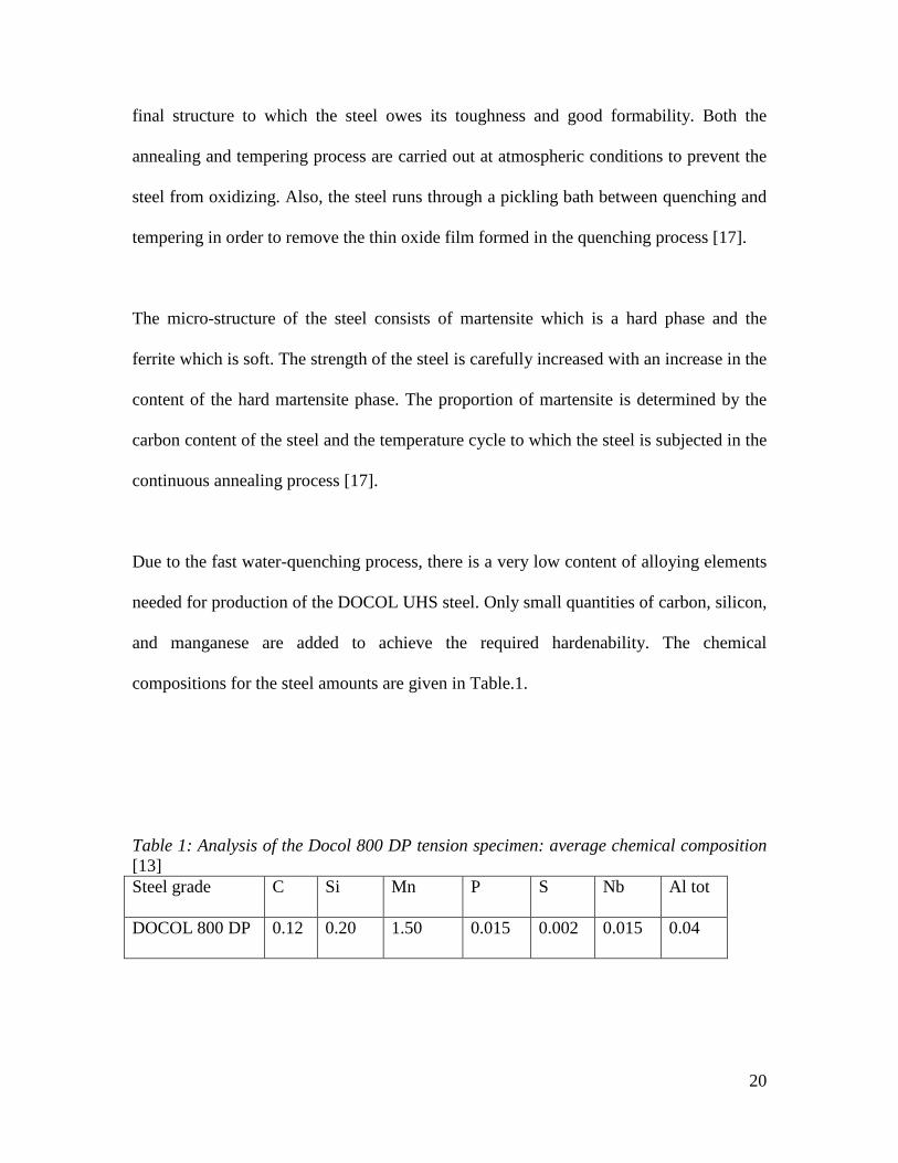
Due to the fast water-quenching process, there is a very low content of alloying elements

needed for production of the DOCOL UHS steel. Only small quantities of carbon, silicon,

and manganese are added to achieve the required hardenability. The chemical

compositions for the steel amounts are given in Table.1.

Table 1: Analysis of the Docol 800 DP tension specimen: average chemical composition [13] Steel grade C Si Mn P S Nb Al tot

DOCOL 800 DP 0.12 0.20 1.50 0.015 0.002 0.015 0.04

21

DOCOL UHS steel is suitable for many applications in the automotive industry and in

particular safety parts, like side-impact beams, because of its amplified strength [17].

With the safety of passengers and plant workers in mind, engineers have to choose the

appropriate steel for the job according to its mechanical properties. These properties

enable them to design and manufacture products that are safe and reliable.

2.2 LOW CYCLE FATIGUE

2.2.1 INTRODUCTION

Repeated loading in conjunction with rolling contact between materials, produces rolling

contact fatigue. The majority of failures in machinery and structural components are

attributed to fatigue failure. Such failure generally takes place under the influence of

cyclic loading.

In 1829 a German mining engineer known as W.A. J. Albert studied the performance of a

hoist chain made of iron under repeated loads [70]. From Albert’s study, interest in

fatigue began to grow with the ferrous structure being the main focus particularly for

bridges in railway systems. This move was pushed by the tragedy which happened in

1842 when there was a train accident. A comprehensive investigation into the cause of

failure was conducted [70].

22

W. J. M. Rankine recognized the distinctive characteristics of fatigue fracture and then

noted the danger of stress contraction in machine components [61]. It soon led to an

investigation of the weakening of materials due to crystallization of the underlying

microstructure.

August Wohler used full scale railway axles to draw up a stress versus cycles to failure

curve, now known as an S-N curve to quantify fatigue [75]. Wohler also noticed that steel

exhibits a so-called endurance limit, which resulted in no damage below the stress value

[75]. Then Bauschinger uncovered a breakthrough in quantifying fatigue which showed

that the limit of the elasticity on the first compression loading is less than the initial

tension loading which is called the Bauschinger effect [75].

The first tests were performed with a fully reversible cycle, which meant that the tensile

and compressions stressing was equal. This was not practical because it did not resemble

a real life scenario and a way had to be developed to offset the normal Wohler type curve.

This was first attempted by Goodman, Soderberg and Gerber [70]. Their work was based

on the ultimate tensile stress or yield stress and endurance limit stress or fatigue strength.

Ewing and Rosenhuim in 1900 and Ewing and Humphrey in 1903 [25], showed that slip

bands developed in many grains of the polycrystalline material. These slip bands broaden

as cyclic deformation continues and leads to extrusion and intrusions on the surface.

23

Although fatigue of metals caused by the slow growth of microscopic flaws was

documented in the works of Ewing and Humphrey, the mathematical framework for the

quantitative modelling of fatigue failure was still not available [25].

The stress analysis of Inglis in 1913 and the energy concept of Griffith in 1921 provided

the mathematical tool for quantitative treatment of fracture in brittle solids [25].

Characterizing fatigue failure of metallic materials was still impossible until Irwin in

1957, who showed that, the amplitude of the stress singularity ahead of a crack could be

expressed in a scalar quantity known as the stress intensity factor, K [25, 43, 70].

Paris, Gomes and Anderson in 1961 suggested that the increment of fatigue crack per

stress cycle da/dN could be related to the range of the stress intensity factor, ΔK, during

the constant amplitude cycle loading [25, 43, 70].

Further development was done independently by Coffin and Manson in 1957 who

proposed that plastic strains are responsible for fatigue damage [25, 43, 70]. This led to

the understanding of why metal parts subjected to repetitive or cyclic stresses fail at a

much lower stress than the fracture stress corresponding to monotic tension stress [25].

More studies provided valuable information on substructural and microstructural changes

responsible for cyclic hardening and softening characteristic of materials and on the role

of such a mechanism in influencing the nucleation and growth of fatigue cracks [70].

24

Parts like turbine blades undergo cyclic loading causing structural deterioration which

can lead to failure [46].

There are several studies which look at damage at a given time during the operational

history of the structure. This is typically called diagnostics and involves detection,

location and isolation of damage from a set of measured values [46].

The development of reliable life prediction models which are capable of handling

complex service conditions are a challenge to engineers [11]. This is due to the

application of fatigue concepts to a practical situation often involving semi-empirical

approaches. Most recently studies have considered a system-approach to the modelling of

damage growth based on differential equations while others have used physics-based

models [74].

During the machine service, the machine parts undergo random load distribution which

affects the dynamic response of materials. Therefore, an investigation of the dynamic

response of fatigue damaged 6061-T6 aluminium alloy and AISI 4140T steel specimens

due to cyclic plasticity and subjected to impact loading was conducted. The investigation

found was that fatigue damage affects the quasi-static behaviour of steel more

significantly than that of aluminium [64].

25

It is well known that welds are the weak links in any structure. So, it is of utmost

importance to characterize the mechanical properties of welds and the changes in the

microstructure that occur in welds on exposure to high temperatures [22].

Morrow’s modified Manson–Coffin equation and Smith–Watson–Topper’s damage

equation investigated fatigue in spot welds using elasto-plastic finite element analysis

[80]. It was found that fatigue does exist in the tensile shear spot weld [80].

As a result, it was found that fretting fatigue limit of grooved specimen could be

evaluated on the basis of the maximum axial stress near the contact edge [45].

The formation and propagation of crack networks in thermal fatigue is predicted using

probabilistic models. They are based on a random distribution of sites where cracks

initiate on the shielding [52].

2.3 PIEZOELECTRIC 2.3.1 INTRODUCTION

In the 18th century crystals of certain minerals known as pyroelectricity were discovered.

These crystals had the ability to generate electrical charges when heated [26]. In 1880,

brothers; Pierre and Jacques Curie, predicted and demonstrated the piezoelectric

phenomenon using common place items such as tinfoil, glue, wire, magnets, and a

26

jeweller’s saw. Their experiment consisted of a measurement of the surface charges

appearing in specially prepared crystals, which generated electrical polarization from the

mechanical stress. This discovery was dubbed as piezoelectricity in order to distinguish it

from other scientific phenomenological experiences such as contact electricity (friction-

generated static electricity) and pyroelectricity (electricity-generated from crystal by

heating) [10, 26].

However, the brothers did not predict that crystals that exhibit direct piezoelectric effect

(electricity from applied stress) would also exhibit the converse piezoelectric effect

(stress in response to an applied electric field). This property was mathematically

deduced from fundamental thermodynamic principles by Lippmann [10, 26]. Pierre and

Jacques experimentally confirmed the existence of the converse effect. They went on to

obtain a quantitative proof of the complete reversibility of electro-elasto-mechanical

deformation in piezoelectric crystals.

It was after two years of interactive work within the European community that the core of

piezoelectric application was broken down into: 1. the identification of piezoelectric

crystals on the basis of asymmetric crystal structure; 2. the reversible exchange of

electrical and mechanical energy; and finally the usefulness of thermodynamics in

quantifying complex relationships such as mechanical, thermal, and electrical variables.

In 1910 the standard reference work was formulated using a thermodynamics potential of

piezoelectricity [10, 26]. Piezoelectrics were found to be obscure even among

27

crystallographers, the mathematics was complicated, and no publicly visible application

was found.

The first practical application for piezoelectric devices was sonar, first developed during

World War I. A French engineer Paul Langevin and his co-workers developed and

perfected an ultrasonic submarine detector [10, 26]. The detector consisted of a

transducer made of thin quartz crystals carefully glued between two steel plates, and a

hydrophone to detect the returned echo. By emitting a high-frequency chirp underwater

and measuring the depth by timing the return echo, one could calculate the distance to the

object [10, 26]. The success of sonar stimulated intense development in resonating and

non-resonating devices.

It is desirable to control the vibration and stabilise the structure from its resonating

frequency. This will lead to a reduction in critical failure of key structural components.

Hence, the development of active vibration control was considered [54].

Tzou and Tseng discovered that by utilizing direct and converse piezoelectric

characteristics, the integrated piezoelectric sensor or controller could be used in

monitoring vibrations due to mechanical stress [76, 77, 78]. This could also actively and

directly constrain any undesirable vibration of flexible components by simply injecting

high voltage. Hamilton’s principle and variation equations are used to derive the thin

piezoelectric hexahedron element.

28

The stacking of quadrangular solids of the piezoelectric element was investigated by

Tsou and Tseng then later another layer to the piezoelectric element was added [76, 77,

78]. The analysis was a problem because the results were so cumbersome that they

required a technique known as Guyan reduction to reduce the number of degrees of

freedom, cited in [77].

Further research on the development of mathematical models simulating plates and shell

structure with embedded piezoelectric film were conducted. A multi-layered composite

piezoelectric Kirchhoff analysis was derived to accommodate the thickness as well as the

thin shell structure, cited in [38, 40].

There are two approaches which can be considered in active control using a piezoelectric

sensor. Firstly, it assumes that the signal from the sensor be an electric current, hence the

closed-circuit mode. Secondly, Wang et al. assumed that the signal from the sensor be a

potential change causing it to be an open circuit mode [15, 76, 77].

Figure 1.0 Block diagram of a Smart Structure [26]

29

Miller used a closed circuit approach in a study for dynamic piezoelectric structures to

show that the structure should be passive-meaning, free from any piezoelectric control at

zero amplifier gain [54]. Then research shifted to the open circuit that showed the

possibility of structural control through piezoelectric elements.

It was shown that the static deflections of the cantilever plate can be controlled by

applying the suitable voltage to the piezoelectric element cited in [36]. These studies still

did not look into the bearing caused by the active model at zero gain.

Further investigation done by Tzou and Tseng developed a model which showed that

control forces persist at zero amplifier gain when the current active control model of the

open circuit mode is used [77]. It prompted Kekana to develop a base for the control

model which resembles a passive structure at zero gain [40]. However, the results

showed that piezoelectric effects persist at zero gain, contrary to the requirements

stipulated in Miller [54].

There are several studies which look at damage at a given time during the operational

history of the structure. This is typically called diagnostics and involves detection,

location and isolation of damage from a set of measured values cited in [23, 46, 83].

Nonlinear vibration analysis of a directly excited cantilever beam is modelled as an

inextensible viscoelastic Euler–Bernoulli beam as part of physics based model [51]. The

analytically derived frequency response was experimentally verified through harmonic

30

force excitation. Results demonstrate that increasing the excitation amplitude or

decreasing damping ratio can cause a minor decrease in the nonlinear resonance

frequency despite the significant increase in the amplitude of vibration due to reduced

damping [51].

Vibration problems for continuous systems with damping effects, including modal,

transient, and harmonic and spectrum response have also been analyzed. It involved

modal analysis of eigenvalues and eigenfunctions [79].

It has also been found that an effective way of investigating the efficiency of system

identification can be done using the Observer Kalman Filter Identification (OKFI)

technique in which the numerical simulation and experimental study of active vibration

control of piezoelectric smart structures is conducted [81].

A new coupled approach of combining EMI technique and a reverberation matrix method

has been investigated, which help quantitatively correlate damages in framed structures

with high-frequency signature for structural health monitoring [82].

31

2.3.2 OPERATIONAL PRINCIPLES

The way piezoelectric material operates depends mainly on the way it is cut. There are

three main modes of operation which can be distinguished: transverse, longitudinal, and

shear.

Transverse effect

Force is applied along a neutral axis (y) and the charges are generated along the (x)

direction, perpendicular to the line of force. The amount of charge depends on the

geometrical dimensions of the respective piezoelectric element [58].

Longitudinal effect

The amount of charge produced is proportional to the applied force and is independent of

size and shape of the piezoelectric element. Using several elements that are mechanically

in series and electrically in parallel is the only way to increase the charge output [58].

Shear effect

The charges produced are proportional to the applied forces and are independent of the

element’s size and shape. With the transverse effect it is possible to adjust the sensitivity

of the force applied and the element dimension [58].

32

2.3.3 ELECTRICAL PROPERTIES

The piezoelectric transducer produces high DC output impedance which is used as a

voltage source. The voltage (V) at the source is directly proportional to the applied force,

pressure, or strain [58]. The output signal is then related to this mechanical force as if it

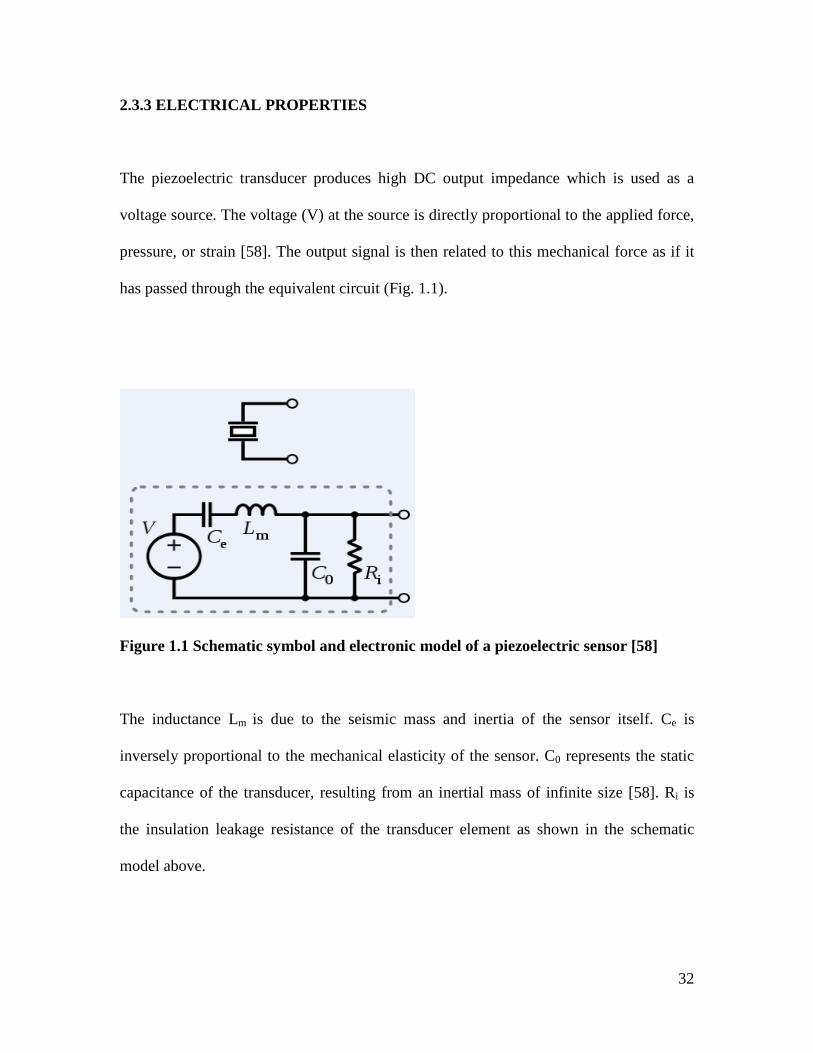
has passed through the equivalent circuit (Fig. 1.1).

Figure 1.1 Schematic symbol and electronic model of a piezoelectric sensor [58]

The inductance Lm is due to the seismic mass and inertia of the sensor itself. Ce is

inversely proportional to the mechanical elasticity of the sensor. C0 represents the static

capacitance of the transducer, resulting from an inertial mass of infinite size [58]. Ri is

the insulation leakage resistance of the transducer element as shown in the schematic

model above.

33

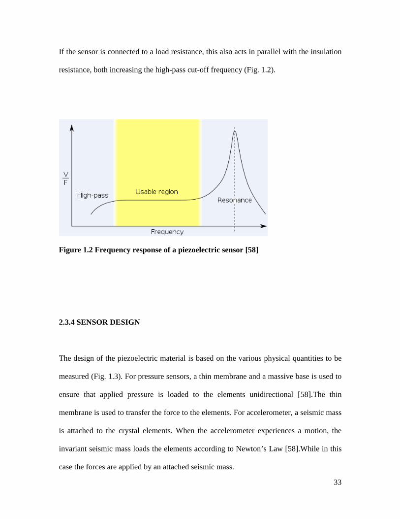
If the sensor is connected to a load resistance, this also acts in parallel with the insulation

resistance, both increasing the high-pass cut-off frequency (Fig. 1.2).

Figure 1.2 Frequency response of a piezoelectric sensor [58]

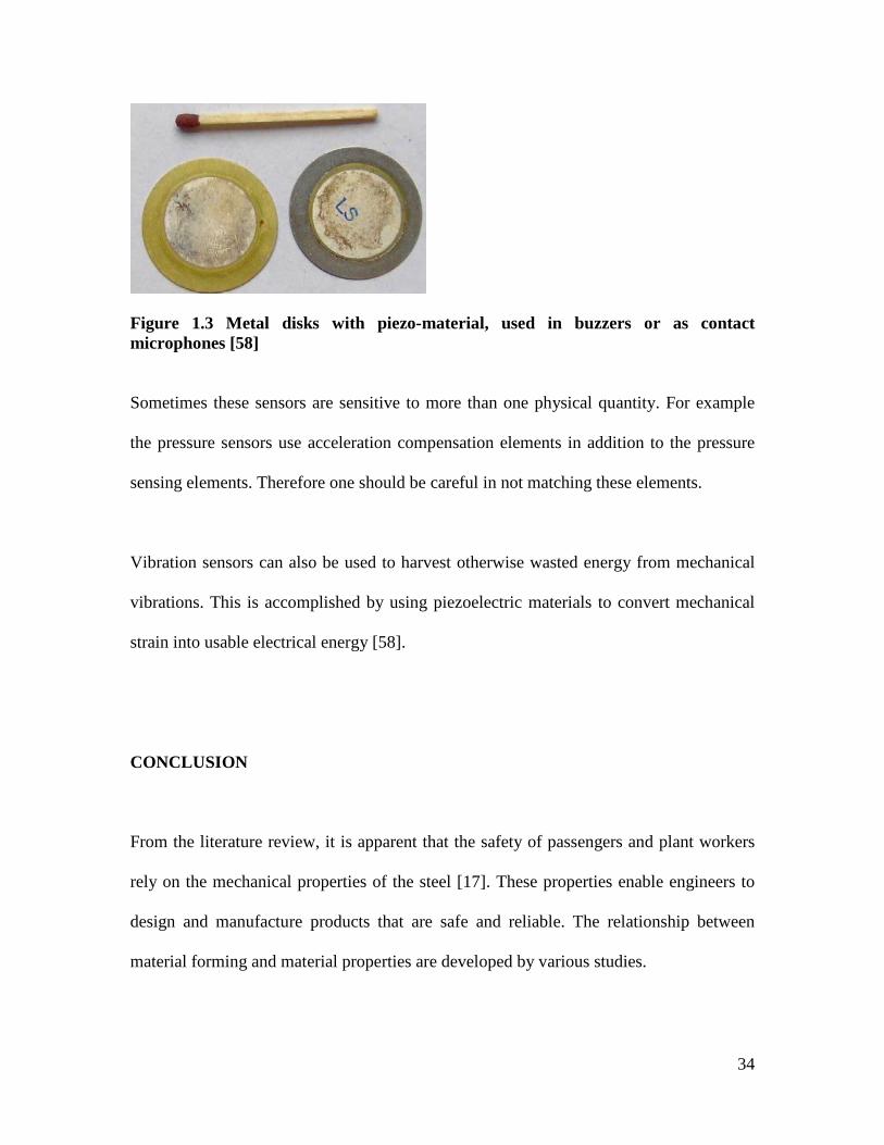
2.3.4 SENSOR DESIGN

The design of the piezoelectric material is based on the various physical quantities to be

measured (Fig. 1.3). For pressure sensors, a thin membrane and a massive base is used to

ensure that applied pressure is loaded to the elements unidirectional [58].The thin

membrane is used to transfer the force to the elements. For accelerometer, a seismic mass

is attached to the crystal elements. When the accelerometer experiences a motion, the

invariant seismic mass loads the elements according to Newton’s Law [58].While in this

case the forces are applied by an attached seismic mass.

34

Figure 1.3 Metal disks with piezo-material, used in buzzers or as contact microphones [58]

Sometimes these sensors are sensitive to more than one physical quantity. For example

the pressure sensors use acceleration compensation elements in addition to the pressure

sensing elements. Therefore one should be careful in not matching these elements.

Vibration sensors can also be used to harvest otherwise wasted energy from mechanical

vibrations. This is accomplished by using piezoelectric materials to convert mechanical

strain into usable electrical energy [58].

CONCLUSION

From the literature review, it is apparent that the safety of passengers and plant workers

rely on the mechanical properties of the steel [17]. These properties enable engineers to

design and manufacture products that are safe and reliable. The relationship between

material forming and material properties are developed by various studies.

35

There were several studies which looked at damage during the operational history of the

structure. These typically looked at the diagnostics which involve detection, location and

isolation of damage from a set of measured values.

The literature also showed how piezoelectric materials operate in accordance to the way

they are cut. Therefore the designs of piezoelectric materials are based on the various

physical quantities to be measured. It was shown that the static deflections of the

cantilever plate can be controlled by applying suitable voltage to a piezoelectric element

(Fig. 1.1).

These findings suggest there is value in examining low cycle fatigue using new

sophisticated sensors known as piezoelectric sensors.

36

Chapter 3

UNI-AXIAL LOADING

The main objective of this chapter is to investigate the different testing rigs and then

identify which driving system can be used for standard tensile testing. The purpose of the

tensile test is to obtain measures of material properties found from sampling material

tested.

This standard engineering procedure is useful in characterizing the relevant elastic and

plastic variables relating to the mechanical behaviour of the materials.

A material processing technique is also presented. This preparation allows for the shaping

of the specimen either by cold rolling or hot rolling into a rectangular cross-section.

37

3.1 TENSILE TESTING MACHINES

Laboratory material testing started in Southwark, London by David Kirkaldy in 1865 [13,

14, 16], which were based simply on loads being applied to test specimens by means of

testing machines. Now there are a variety of testing machines which can be used in

carrying out the experiments required, depending on their purpose, configuration, size,

capacity, and versatility.

In the period between 1900 and 1920 a simple type of testing machine was built [13, 14,

16]. It consisted of a basic configuration of just applying the load to the specimen and

then measuring the load. This still plays an essential part in testing machines today.

Depending on the design of the machine, these parts can either be entirely separated or

superimposed on one another.

3.1.1 Screw Driven Testing Machine

In the case of a screw-driven testing machine, the specimen is extended by having one

grip fixed to the frame of the machine while the other grip is movable on the crosshead.

The crosshead is displaced by a motor that turns two large screws located at either end of

the crosshead which applies the load on the specimen.

In 1946 Instron Corp. introduced an improved and sophisticated electronic system testing

machine which was based on the technology of a vacuum tube [20, 31]. This saw a

38

screw-driven machine using electronics to control and measure the loads and

displacements, making the machine much more versatile (Fig. 3.1 (a)). The advantage of

a screw-driven testing machine is that, the crosshead cannot move very fast, usually a few

millimeters per second at most. This minimizes mistakes caused by the grips moving

together rather than apart.

Figure 3.1 (a) The Screw-Driven Testing Machine, (b) Servohydraulic Testing Machin [31, 55]

39

3.1.2 Servohydraulic Testing Machine

Around 1958, a transistor technology and closed-loop automation concept was used by

the forerunner of the MTS Systems Corp to develop a high-rate testing system using a

double action hydraulic piston [20, 55]. This resulted in the second type of testing

machine known as the servohydraulic testing machine (Fig. 3.1 (b)).

In this case, the displacement of the grips is imposed by high pressure oil driving a

piston. The actual position of the piston is measured by a sensor which generates a

voltage proportional to its position [13, 14, 16]. A separate signal generator produces a

voltage that corresponds to the desired position of the piston. If the two voltages are

different, valves are operated electronically so that the high pressure oil moves the piston

to the desired position.

The advantage of the machine is that, it can operate in various modes such as constant

displacement rate or constant rate of load application, by simply changing the way the

control voltage is generated [13, 14]. This flexibility makes the machine capable of

performing a wide variety of tests. However, the flexibility also means that the controls

are more complex. The piston can be driven at very high displacement rates by the high-

pressure oil rates at an average 10 m/s.

40

3.2 EXPERIMENTAL METHODS

3.2.1 Materials

A metal alloy is usually melted together with two or more chemical elements where the

bulk of the material consists of one or more metals. This has produced a wide range of

metallic and non-metallic chemical elements used in alloying a principal engineering

metal. Some commonly used elements are boron, carbon, magnesium, silicon, etc. The

amounts and combinations of alloying elements used with various metals have major

effects on their strength, ductility, temperature resistance, corrosion resistance, and other

properties [13, 14].

3.2.2 Specimen preparation for Micro-structure

For the examination of the microstructure of metals the surface of the specimen must be

correctly grounded, polished and etched. The selection of the specimen to be examined

plays a vital role in knowing the complete picture of the specimen. If a casted material is

to be examined, it is important to take several micro-sections in order to see the grain

structure at the centre and the edges. When the component is rolled, it is advantageous to

take specimens in the direction of working to see if there is any directional distribution of

the constituents.

41

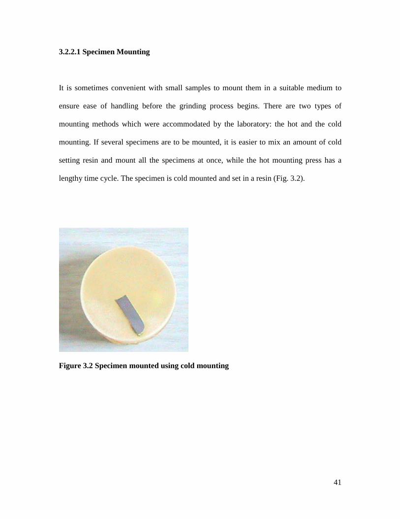
3.2.2.1 Specimen Mounting

It is sometimes convenient with small samples to mount them in a suitable medium to

ensure ease of handling before the grinding process begins. There are two types of

mounting methods which were accommodated by the laboratory: the hot and the cold

mounting. If several specimens are to be mounted, it is easier to mix an amount of cold

setting resin and mount all the specimens at once, while the hot mounting press has a

lengthy time cycle. The specimen is cold mounted and set in a resin (Fig. 3.2).

Figure 3.2 Specimen mounted using cold mounting

42

3.2.2.2 Specimen Preparation

Pre-grinding is carried out prior to polishing and it consists of rubbing a suitably flat

surface of a specimen on increasingly fine grinding papers. The operation is carried out

on a rotating grinding wheels bench using silicon carbide paper and water as a lubricant.

The silicon carbide paper range generated from 180 grit (which is coarse) up to 1000 grit

(which is fine). After each grade paper has been used, the specimen is rinsed and turned

through 90o before moving on to the next grade paper. This ensures that the scratches in

one direction are totally eliminated by the operation on the next paper.

After the pre-grinding stage the specimen is washed thoroughly with soap and dried,

preferably with alcohol.

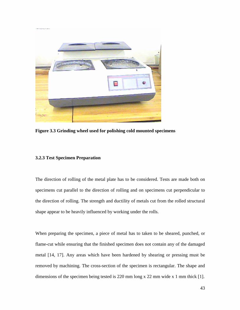
The polishing is performed on a rotating wheel (Fig. 3.3) covered with a selvyt clothe.

The polishing agent used is a diamond paste at ¼ micron. Finally the specimen is etched

using a nitric acid based solution. This corrodes the metal showing the crystal structure of

the metal.

43

Figure 3.3 Grinding wheel used for polishing cold mounted specimens

3.2.3 Test Specimen Preparation

The direction of rolling of the metal plate has to be considered. Tests are made both on

specimens cut parallel to the direction of rolling and on specimens cut perpendicular to

the direction of rolling. The strength and ductility of metals cut from the rolled structural

shape appear to be heavily influenced by working under the rolls.

When preparing the specimen, a piece of metal has to taken to be sheared, punched, or

flame-cut while ensuring that the finished specimen does not contain any of the damaged

metal [14, 17]. Any areas which have been hardened by shearing or pressing must be

removed by machining. The cross-section of the specimen is rectangular. The shape and

dimensions of the specimen being tested is 220 mm long x 22 mm wide x 1 mm thick [1].

44

3.2.4 Testing Conditions

The material to be tested for mechanical behaviour had to be selected using the ASMT

standards for materials [1]. For the testing conditions, one had to consider the conditions

of the material at the time of testing and to keep the ambient conditions [1] (Table 2).

Depending on the temperature at which the tests are conducted, they normally produce

three general classes of tests. The first class of tests are carried out at normal atmospheric

or room temperature, while the second class of tests are made to determine material

properties, such as brittleness of steel, at very low temperatures, as might be required in

the development of high-altitude aircrafts. The final class of tests are carried out at

elevated temperatures as in the development of rockets, jet engines, to elevate the

strength, ductility and creep of the material under such conditions [14, 20].

The mechanical property of materials is heavily affected by moist conditions [1]. This

allows for a detailed specification for testing the make-up of the specimen in relation to

its physical condition. In conducting the tensile test, the manner of holding, gripping,

supporting, or bedding the specimen plays a key role and therefore, it had to receive good

attention.

Table 2: Initial conditions experienced during testing Specimen Initial Temperature 23

Room Temperature 23

45

3.3 QUASI-STATIC MECHANICAL TEST

3.3.1 Tensile Test/ Compression Test

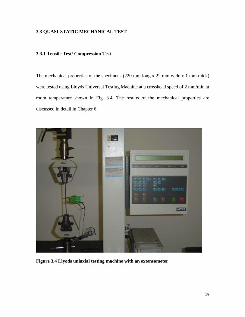
The mechanical properties of the specimens (220 mm long x 22 mm wide x 1 mm thick)

were tested using Lloyds Universal Testing Machine at a crosshead speed of 2 mm/min at

room temperature shown in Fig. 3.4. The results of the mechanical properties are

discussed in detail in Chapter 6.

Figure 3.4 Llyods uniaxial testing machine with an extensometer

46

3.3.2 Optical Microscope

An optical microscope is used for examining and photographing the metallurgy of the

specimen (Fig. 3.5).

A horizontal set of light rays is emitted from the illuminator and is diverted downwards

by means of a glass reflector, through the objective lens to the metal specimen. The light

which is reflected from the specimen (Fig. 3.2) surface passes back through the objective

to form an enlarged image. The light then passes through the eyepiece lens to form a

further magnified image for visual examination. The magnification used was 800X for

clarity of the image. The metallurgical results are discussed in detail in Chapter 6.

Figure 3.5 Microscope with the magnification of 800 X lens

47

CONCLUSION

The proposed experimental testing was carried out using Lloyd’s tensile testing machine,

to produce experimental data which form the mechanical properties for the metal. The

process was operated at 2mm/min to insure a uniform distribution load across the

rectangular plate and standard testing procedures were observed.

The study used testing technology to further extract the material properties of a

rectangular specimen, focusing mainly on the tension and compression of structures until

failure and results producing the stress range. The ambient temperature was maintained

during testing so that external influences could be neglected.

The kind of technology and knowledge used has made it possible for the study to classify

the material profile under examination. It can be clearly stated that the material under

testing (DOCOL 800DP – steel) is ductile and the stress range falls within the material as

given in the literature [17].

The rectangular plate was cold rolled during material processing and the steel was

annealed at temperatures between 750-850oC and therefore harden by being quench at a

uniformly distributed load in water [17].

48

Chapter 4

CYCLIC LOADING

The previous chapter went into detail describing the experimental methods which must be

adhered to for successfully testing structures under tension. It dealt with different

machinery which could be used to develop the experimental mechanical properties.

However, this does not cater for a dynamically loaded structure. Therefore, this chapter

concentrates on fatigue failure of structures under cyclic loading. The fact is that dynamic

loading conditions heavily impact on the experimental data. It is important to provide

engineering designers with data to formulate a fairly precise estimation of the load that

the structure or machine can handle. Therefore, testing becomes a necessity for

establishing the cause of failure and verifying the specifics which were not confirmed.

In this situation testing data requires a deeper understanding of the strain measuring

instrument. This has helped to form the basis of the investigation in the monitoring of

structural degradation. Low cycle fatigue can cause significant plastic deformation in a

material due to its repeated loading system. This normally causes a surge in a fatigue

cracking.

49

The two measuring instruments are measured against each other to find the most accurate

one. A data acquisition system is also programmed to capture real-time action from the

experiments. Each specimen follows a given stress amplitude, completely reversible.

That is, the mode of testing is strain controlled at ± 5% instead of stress controlled.

This dynamic analysis has made it possible to determine the behaviour of structures.

4.1 FATIGUE BENDING MACHINES

4.1.1 Cantilever Beam Machine

This machine is capable of producing either completely reversed cyclic stresses or non-

zero mean cyclic stresses by simply positioning the specimen to the clamping vise with

respect to the mean displacement position of the crank drive (Fig. 4.1). It also relies on

controlled geometric deflections from the rotating eccentric crank to keep the alternating

strain level at zero. The geometric changes in the apparatus alter the length of the

connecting rod from the eccentric drive to give different mean deflections and thus

different mean stresses [20].

50

Figure 4.1 Cantilever Beam Machine [31, 55]

4.1.2 Rotating Beam Machine

The R.R. Moore – type machines are the most commonly used rotating beam machines in

which a specimen with a round cross section is subjected to a dead-weight load while

bearings permit rotation (Fig. 4.2). A given point on the circular test section surface is

subjected to sinusoidal stress amplitude from tension on the top to compression on the

bottom with each rotation. These machines can operate up to 10 000 rpm [20].

51

Figure 4.2 R.R. Moore Rotating Beam Machine [31, 35]

4.2 EXPERIMENTAL METHODS

4.2.1 Materials

The cross section of the specimen is rectangular. The shape and dimensions of the

specimen being tested are 220 mm long x 22 mm wide x 1 mm thick [1].

4.2.2 STRAIN MEASURING EQUIPMENT

4.2.2.1 Strain gauge

For the conversion of mechanical motion into an electronic signal a strain gauge had to

be selected. This strain gauge was connected to a Wheastone Bridge circuit as a resistor

[73].

52

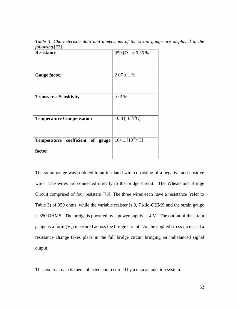
Table 3: Characteristic data and dimensions of the strain gauge are displayed in the following [73] Resistance 350 [Ω] ± 0.35 %

Gauge factor 2.07 ± 1 %

Transverse Sensitivity -0.2 %

Temperature Compensation 10.8 [10-6/oC]

Temperature coefficient of gauge

factor

104 ± [10-6/oC]

The strain gauge was soldered to an insulated wire consisting of a negative and positive

wire. The wires are connected directly to the bridge circuit. The Wheatstone Bridge

Circuit comprised of four resisters [73]. The three wires each have a resistance (refer to

Table 3) of 350 ohms, while the variable resister is 0, 7 kilo-OHMS and the strain gauge

is 350 OHMS. The bridge is powered by a power supply at 4 V. The output of the strain

gauge is a form (Vo) measured across the bridge circuit. As the applied stress increased a

resistance change takes place in the full bridge circuit bringing an imbalanced signal

output.

This external data is then collected and recorded by a data acquisition system.

53

4.2.2.2 Piezoelectric sensor

The Piezoelectric sensor was selected to be used for measuring strain that occurs on the

thin plane. The sensor is attached to the specimen by means of an adhesive. An

advantage of using piezoelectric is that they generate their own voltage; therefore it was

not connected to the Wheatstone Bridge Circuit or is the signal amplified.

The output from the piezoelectric sensor is a voltage reading (see Table 4).

Table 4: Characteristics of a Quick-Mount bending performance actuator [58] Piezo Material

5A4E

Weight (grams)

2.3

Stiffness (N/m)

760

Capacitance (nF)

Parallel Operation

52

Rated Voltage (Vp)

Parallel Operation

± 90

Resonant Frequency (Hz)

275

Free Deflection (µm)

± 315

Blocked Force (N)

± .31

54

4.2.3 Strain Acquisition System

When the apparatus is in motion, the strains induced are sent through a laptop DAQ card

which converts the analog to digit signal. Data is acquired through two channels in the

form of voltage (V) (Fig. 4.3).

With the piezoelectric sensor, different conditioning equations were used. They consisted

of change in electric current density. This means that the Lab-View program is set

differently as compared to the strain gauge packages (Fig. 4.3).

Figure 4.3 Illustrates the conditioning of the signal using Lab-View

The DAQ card processes the results then they are stored in a file until the experiment is

over. The voltage signal is basically translated to forces, by a conversion system related

55

to strain gauge theory and Lab-View in Fig. 4.5. This allows one to determine the stress-

strain curve during cyclic testing. Once the behaviour has stabilised a closed stress- strain

hysteresis loop is formed during each strain cycle. The area inside the hysteresis loop is

the energy absorbed per unit volume of the material. The energy mostly dissipates as heat

energy.

Figure 4.5 Block Diagram for Data Acquisition

4.2.4 Test Condition

According to ASTM standard E4606, the ambient temperature must be kept at constant

room conditions [1]. This assists in preventing temperature effects in the experiment

being conducted. When the initial conditions are stable at room temperature, the

specimen used has a length of 220mm, width of 22mm and thickness of 1mm. The

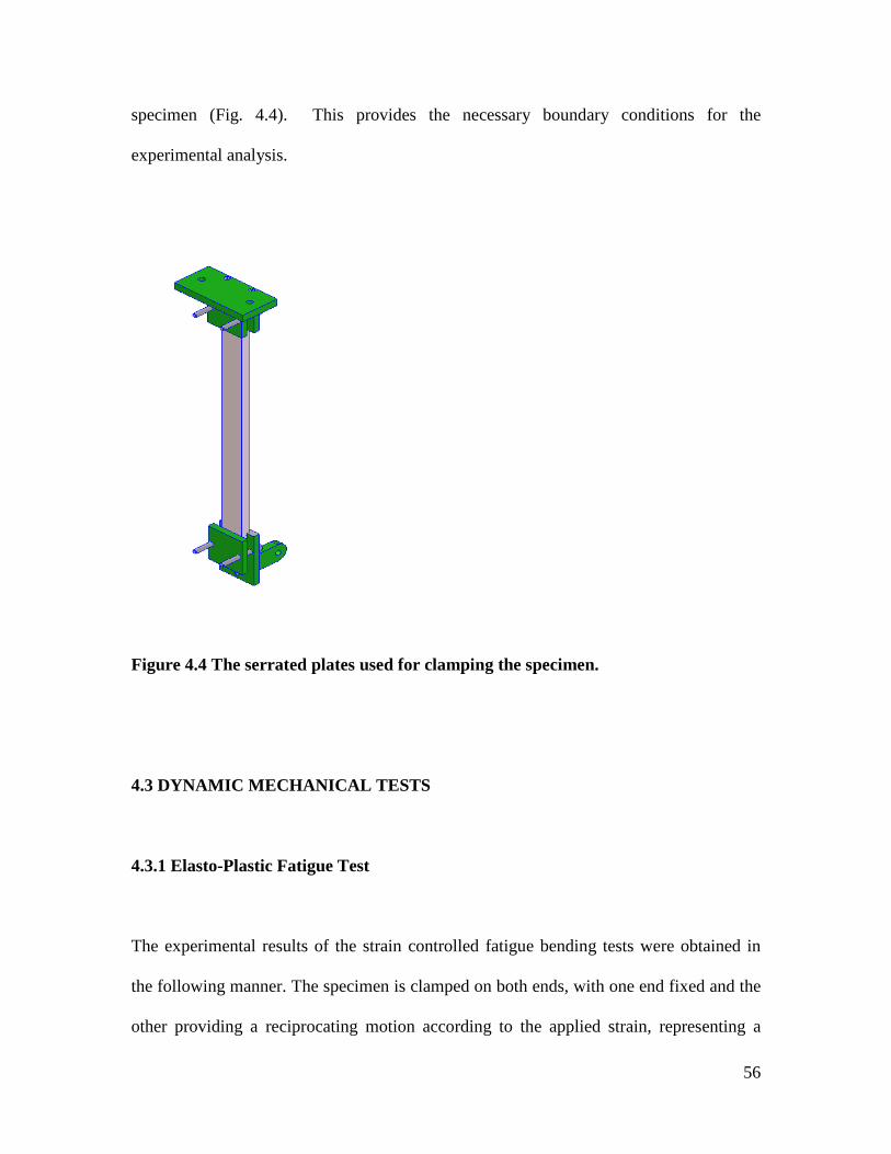
fatigue bending machine has two serrated plates which are used for clamping the test

56

specimen (Fig. 4.4). This provides the necessary boundary conditions for the

experimental analysis.

Figure 4.4 The serrated plates used for clamping the specimen.

4.3 DYNAMIC MECHANICAL TESTS

4.3.1 Elasto-Plastic Fatigue Test

The experimental results of the strain controlled fatigue bending tests were obtained in

the following manner. The specimen is clamped on both ends, with one end fixed and the

other providing a reciprocating motion according to the applied strain, representing a

57

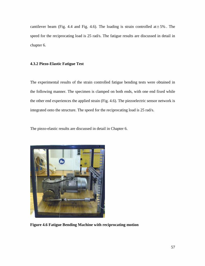
cantilever beam (Fig. 4.4 and Fig. 4.6). The loading is strain controlled at %5± . The

speed for the reciprocating load is 25 rad/s. The fatigue results are discussed in detail in

chapter 6.

4.3.2 Piezo-Elastic Fatigue Test

The experimental results of the strain controlled fatigue bending tests were obtained in

the following manner. The specimen is clamped on both ends, with one end fixed while

the other end experiences the applied strain (Fig. 4.6). The piezoelectric sensor network is

integrated onto the structure. The speed for the reciprocating load is 25 rad/s.

The piezo-elastic results are discussed in detail in Chapter 6.

Figure 4.6 Fatigue Bending Machine with reciprocating motion

58

CONCLUSION

The in-house fatigue rig (Fig. 4.6) was used for the dynamic testing of the rectangular

plate in a controlled ambient temperature environment to minimise any external influence

which can be caused by heat.

The experiments were carried out to monitor structural degradation of plates. The results

are used to determine the material behaviour under continuous loading systems.

The application of this fatigue rig is to cyclically load a ductile structure in order to

produce cyclic curves.

The collection of the experimental data was done using a computer data acquisition

system. The system was programmed using Lab-View to convert signals from the two

sensors into values (Fig. 4.3). Furthermore, the two measuring instruments used for the

measuring of deflection were directly linked to the real-time acquisition system.

The experiments conducted provide the study with fatigue data for the rectangular

DOCOL 800DP specimens. This makes it possible to track and monitor the cause of

failure during continuous loading.

Using these experiments, the cyclic profile for DOCOL 800DP steel under cyclic speeds

of 25 rad/s was obtained.

59

Chapter 5

TECHNICAL BACKGROUND

This chapter presents the mathematical relationship for expressing stress and strain

behaviour at particular points which deals with the elastic behaviour of a solid that obeys

Hooke’s Law [16]. The theory of plasticity is well presented within the chapter. The

plastic deformation was not easily measured; constants and strain hardening were

difficult to accommodate without introducing any mathematical complexities [6]. The

theories were formed for describing the mechanical behaviour of the metal based on the

assumption that the metal is homogenous and isotropic.

Damage is said to be caused by movement and accumulation of dislocation in metals.

Dislocations are caused by impurities, heating and repeated loading of the metal.

Therefore scientists and engineers tried to characterise fracture by simply using

mechanical variables, although this approach had its shortcoming which were improved

by Kachanov who introduced damage variables [33].

This chapter further presents damage variables which are coupled with elastic and plastic

behaviour of the metal that produces a degradation model at each stage of the fatigue life

60

of the metal using the concept of effective stress and strain. These equations look at

damage from simple tension loading to cyclic loading systems.

Elementary models must be created in order to analyse the experimental results. “The

decoupling of elastic and plastic effects can be justified on the basis of the physics and

chemistry of solids, thermodynamics, and phenomenological experiments. The total

strain may be partitioned or separated into the reversible (or elastic) strain eε and the

irreversible (or inelastic) strain pε without prejudging the nature of the latter strain” [33].

Elastic deformation is associated with a variation in the interatomic distances without

changes in place. “While plastic or inelastic deformation implies slip movement with

modification of interatomic bonds” [33].

elastoplastic framework pe εεε +=

5.1 Elasticity

“All solid materials poses a domain in the stress space within which load variation results

only in a variation of elastic strain” [33]. In linear theory, it is important to choose a

positive potential thermodynamic potential for a quadratic function in the strain tensor

component [33].

εερ ::)( 21 a=Ψ (1)

61

where Ψ denotes the contraction of the tensorial product, ρ is the density and a is the

fourth order tensor which is a component of the elastic moduli depending on the

temperature

σε :A= (2)

now the combination of the isotropic and linearity potential

1)).((1 συσυε TrdE

dE

d ++

= (3)

written in the tensor form

ijijijij Ed

Ed δσυσυε .1 ′+

+= (4)

5.2 Plasticity

“The evolution of the loading surface is governed only by one scalar variable, either the

dissipated plastic work, or the accumulated plastic strain p, or any associated variable

such as the thermodynamic force R. The rules were developed assuming the temperature

to be constant, or at least using criteria which are temperature independent.” [33]

),( Rff σ= (5)

62

Loading function is expressed in )()( Rff Y Γ−= σ “where the function fY indicates of

the yield criterion, and the function Γ introduces hardening through the relation between

the thermodynamics force “R” and the hardening variable chosen (p or wP)” [33]. The

isotropic material “fY”is a function of the stress tensor invariant [33].

Prandtl-Reuss Equation

“The Prandtl-Reuss equation is a flow law in an elastoplastic regime with isotropic

hardening” [33]. Hypothesis of plastic incompressibility: “Plastic strain occurs at

constant volume and flow does not depend on the hydrostatic stress )(31 σσ TrH = . The

function will depend on the deviatoric stress and internal variable,

0=∂∂

H

fσ

Hypothesis of initial isotropy and isotropic hardening: “The loading function depends

only on the invariants J2 and J3 of the deviatoric stress tensor” [33].

21):()( 2

32 σσσσ ′′== eqJ (6)

31):.()( 2

93 σσσσ ′′′=J (7)

63

And associated plasticity and normal hypothesis

)()( 23

eqp dfdd σσλσλε ′=∂

∂= (8)

and now solving for λd ,

21

32 ):()( pp dddR

fddp εελλ ==∂∂−= . (9)

von Mises loading function, is independent from the third variable [33],

0=−−= Yeq Rf σσ (10)

where Yσ is the yield stress during tension. The hardening curve is expressed by the

relation

)()( ppkR ∂∂== ψρ (11)

with R(0) = k(0) = 0, and consistence conditions in the presence of flow (f = 0 and df = 0)

it gives

0)( =′−= dppkddf eqσ (12)

which can be used to plastic multiplier

))()(( pkdfHdpd eq ′== σλ (13)

64

For a material with positive hardening, with 0)( >′ pk , there is no flow except when

eqdσ is positive while for a material with negative hardening 0<eqdσ , the plasticity

multiplier must be zero, and the system x ,

))()(( pkdfHdpd eq ′== σλ (14)

Substitute equation (14) into (8), the flow equation will change to

eq

eqp

pkd

fHdσσσ

ε′

′=

)()(2

3 (15)

to express this equation in stresses only, substitute this equation

)()( 11YeqkRkp σσ −== −− into equation (9) in order to solve for p, then solve equation

(15) taking into account the plasticity equation,

σσ

σσε ′′=

eq

eqeq

pd

gfHd )()(23 Or ij

eq

eqeq

pij

dgfHd σ

σ

σσε ′′= )()(2

3 (16)

elastoplastic framework pe εεε += , the total strain would be by combining equation (4)

and equation (16). Therefore the analytical calculations for this research considered these

two equations (4) and (16).

65

5.3 Elastic Damage

“Damage is not directly accessible to measurements” [33]. It is linked to the phenomenon

representing the variable. Association with the hypothesis of strain equivalent is linked to

deformation coupled with damage [33]. “Damage variable which represents a surface

density of discontinuities in the material leads directly to the concept of effective stress”

[33].

Elastic damage law

εσσ ED =−= )1(~ (17)

Or

eDE εσ )1( −= (18)

where E is Young’s Modulus (elastic modulus free from damage) where elastic modulus

of the damage material EDE ~)1( =− , if the young’s modulus E is known ,

The elastic damage law can be applied

)(1 eED εσ−= (19)

66

and with

eEεσ ~= (20)

Solve the two equations (19 and 20) for D

EED ~1−= (21)

Equation (21) was used to determine the amount of damage accumulated in the material

during tensile testing.

5.4 Fatigue Damage

“Fatigue damage in metals corresponds to nucleation and growth of microcracks,

generally intracrystalline under the action of cyclic loading until the initiation of a

macroscopic crack” [33]. The Palmgreen-Miner linear is based on the assumption that

damage is accumulated additively when it is defined by the associated life ratio Ni/Nfi

where Ni – number of cycle applied under a given load, Nfi –number of cycles to fracture

∑ =i

Fii NN 1)( (22)

67

damage evolution is considered to be linear

FNND = (23)

Damage evolution is linear accumulation rule can apply even when a damage is nonlinear

but it must have a one-to-one relationship between D and Ni/Nfi (24)

Equation (23) was used to obtain the linear damage evolution during fatigue testing. “ the

Palmgreen-Miner linear accumulation law gives good results only for loads for which

there is little variation in the amplitude and mean of the stress”[33], for this reason

equation (23) is used in obtaining fatigue damage models.

5.5 Elastic coupled with Damage

The deformation and damage coupling is used as a starting point for the mathematical

expression. Damage causes the structural stiffness and the material strength to weaken

[33]. For the linear elasticity combined with the isotropic damage the constitutive

equation.

σε :A= (25)

where

)1(~

D−=

σσ (26)

is substituted equation (26) into equation (3) we have

68

DTr

EDE −−

++

=1

)(1

1 συσυε (27)

For damage due to tension assuming that D evolves elastically and has a variable

threshold Dε [33].

=0

*

0

s

dD εε

when Dεε = and 0>= Ddd εε then at zero Dεε < or 0<εd

The initial condition is considered to be 0== DD ε and it should integrate to fracture at

D = 1.

Therefore,

=

+1*s

R

Dεε (28)

Substituting equation (28) into equation (18) and solve for the linear damage models,

]1[1* +

−=

s

R

Eεεεσ where (29)

)1(1

* **

])1[( ++= ssoR s εε defined by 1* =s (30)

Then equation (29) can be used to solve for elastic strains coupled with damage

69

5.6 Plasticity coupled with Damage

The strain equivalent law models damage behaviour together with the material hardening

process [33]. The stress σ is replaced by the effective stress σ~ in the dissipation

potential. The material obeys von Mises criteria and therefore there is isotropic damage.

Substitute )1(

~D−

=σσ into equation (8) and (9) therefore we have,

eqp D σ

σλε′

−=

123

(31)

and )1( Dpr −== λ (32)

The hardening law of the material without damage is given as

)()( rRrrR =∂∂= ψρ [33]. von Mises loading function, is independent from the third

variable which shows the accumulated strain rate due to damage with the consistency

condition when damage was introduced into equation (10)

expressed 0::: =∂∂

+∂∂

+∂∂

= DDfR

Rfff σ

σ (33)

or accumulated strain rate substituted into equation (31), we have

70

0)1(

)()1(

:23

2 =−

+′−−

′D

DrrR

Deq

eq

σ

σσσ (34)

with λ =r , kRD

eq =−−1σ

and λϕ Y

D D

∂∂

=*

and substitute into equation (34), we then get

YrRKrRD D

eq

∂∂

++−= *

)]([)()1( ϕσ

λ

(35)

The boundary conditions for the loading and un-loading criteria

0=λ if 0≤eqσ

0>λ if 0>eqσ

The hardening modulus, in equation (32) is equivalent to the plastic multiplier h(r, D, Y)

as shown in equation (36)

),,()(

1 YDrhfH

Dp eqσλ =

−= (36)

with

YrRkDrRDYDrh D ∂∂+−+′−= *2 )]()[1()()1(),,( ϕ

71

Substitute equation (36) into equation (34), therefore

eqeq

eqeq

p

Dd

DgfHdσσ

σ

σσε

′−

−′=)1(

)1(,()(23 (37)

elastoplastic framework pe εεε += , the total strain including damage models would be

by combining equation (27) and equation (37). These were the two equations which were

used to analyse damage in the material.

CONCLUSION

The outcomes of this chapter are that the constitutive equation can be used to produce

analytical results. These results play an important role when it comes to modelling the

behaviour of the specimen being tested accommodating the elastic and plastic region.

The theory describes the mechanical behaviour of the metal based on the assumption that

the metal is homogenous and isotropic.

Elastic behaviour was considered from a simple phenomenological point which was

established from empirical law.

Damage variables were formulated according to the damage theory. The proposed theory

was capable of coupling elastic behaviour of the metal with its damage process and

likewise with plasticity.

72

These variables were obtained during tension and cyclic testing of the rectangular plate.

The results were used for modelling the analytical solutions which was compared to the

experimental model. This added to the literature by confirming that these equations can

be modelled using analytical models.

The implication is that any form of mechanical behaviour experienced by the structure

can be model using continuum mechanics laws, quantifying the behaviour changed

experienced during the movement of particulars.

73

Chapter 6

RESULTS AND DISCUSSION

In Chapter 6 the results from Chapter 3 and 4 are discussed. The outcomes on the

experimental and analytical investigation of a DOCOL 800DP steel plate are discussed.

The experimental and analytical results are broken down into two parts, the uni-axial and

the cyclic loading systems.

For the uni-axial system, the Lloyd’s testing machine is used to experimentally test the

rectangular DOCOL 800DP steel plate producing load-displacement graphs. The tensile

speed used was 2mm/min at a uniformly distributed load. The deformations experienced

by the material were measured using an extensometer. The results obtained during these

experiments are used in producing the material behaviour for a rectangular DOCOL

800DP steel plate. The results are also used as the standard measure.

The specimens being tested were assumed to be homogeneous therefore material

properties are taken as constant.

74

For the cyclic system, the cyclic curves are plotted from the cyclic tests carried out on

rectangular DOCOL 800DP steel plates. An in-house fatigue bending machine was used

to carry out the cyclic fatigue experiments. A cyclic speed of 25 rad/s was used during

testing. The deformations of the steel plate were measured using two different strain

measuring sensors, the strain gauge and the piezoelectric sensor. These cyclic results

obtained through testing were modified to a standard tensile curve. The vast majority of

fatigue failure methodology and life assessment criteria produce a relationship between

fatigue damage and stress-strain due to cyclic loading [43].

All the results from the tensile and cyclic loading experiments together with the

analytical results are plotted on the graphs below. The strain based approach was

developed to produce accurate means of assessing fatigue life for low cycle fatigue after

the based method seems to fail [43].

6.1 Uni-axial Loading

Three rectangular DOCOL 800DP steel were pulled in tension at 2mm/min until failure

using the Lloyds testing machine. The experimental raw data was measured using an

extensometer and then processed through a DAQ system. The three experimental curves

are given in Fig. 6.1. These sample curves are combined to form a mean tensile curve for

DOCOL 800DP steel under uni-axial loading.

75

The elastic axial strain results from a separation of atoms or molecules in the direction of

loading while they move closer together in the transverse direction [67]. Therefore, the

quantitative measure of elasticity of a material can be expressed as the extent to which

the material can be deformed within the limits of elastic action [67].

As the load carried by the material soon undergoes permanent deformation before failure

due to the properties of the material being promised. The plastic state material deforms

under a constant sustained stress, it involved the concept of limit of deformation before

failure. These plastic strains are caused by slip induced in the material by shear stress.

Figure 6.1 Three samples of DOCOL 800 DP steel under tensile testing using an extensometer

76

Results from Fig. 6.2 were used to obtain the material properties for the DOCOL 800DP

steel plate. The results were verified and were found to be in accordance with the

theoretical results [17].

Fig. 6.2 shows the relationship between elastic and plastic behaviour of the tensile curve

in that a theoretical curve based on purely elastic behaviour ( ijkkijij EEδσυσυε −

+=

1 ) is

compared to the mean of the three tensile curves [16, 33]. Fig. 6.2 shows that a

significant portion of the behaviour of the steel is not elastic. The material DOCOL

800DP steel first behaves elastically as shown by the approximately straight line between

the curves (between 0mm to 0.1mm).

It first behaves elastically ( e

ijε ) within the limits of elastic action then with continued

stressing, there is plastic deformation. Plastic flow ( pijε ) is known to be caused by

dislocations being induced in the metal by the shear stress. These defects move through

the crystal structure of the solid and re-arrange the crystal lattices [67]. This type of

dislocation motion obeys Schmidt’s law which deals with the principle of maximum

plastic resistance [6] and would imply that the yield surface of the solid was convex and

the plastic strain rate was normal to the yield surface [6]. The material reached its

maximum resistance to loading (yield stress) before failure occurred (approximately

1.05GPa).

77

Figure 6.2 Load displacement curves for a rectangular specimen for a fixed beam subjected to a uniformly distributed load with error bars (1 SE)

Fig. 6.3 compares the tensile experiments with analytical curves obtained using equation

(4) and equation (16) (Chapter 5). These equations follow the elastic strain law [16, 33]

which assumes that the conditions of loading are such that strain rate and thermal effects

can be neglected and the material is assumed to be isotropic [18].Using parameters

corresponding to each experiment, three numerical curves were obtained from which a

mean curve was produced. This standard engineering procedure is useful in

characterizing some relevant elastic and plastic variable to the mechanical behaviour of

materials.

78

Figure 6.3 Analysis of DOCOL 800 DP tensile test experiment for a rectangular specimen and analytical results with error bar (1 SE) Any difference between the two curves in Fig. 6.3 is expected to be due to the fact that

the elasto-plastic equations assumed no hardening effect had occurred i.e. ideal

conditions [1, 13]. The experimental curve Fig. 6.3 gives an indication that the material is

not to strain soften rather strain hardening as the stress is increased. This result agrees

with the theory about this material (DOCOL 800DP) which is expected to strain harden

with continued stressing [17]. The strain hardening effect during the plastic deformation

is due to the fact that after minor slips had occurred on the material, it exhibited no

further plastic strain until a higher stress was applied [17, 67]. The maximum shear stress

occurred on the 450 (degree) plane; this led to the specimen failing along the plane.

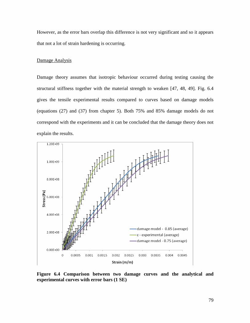
79

However, as the error bars overlap this difference is not very significant and so it appears

that not a lot of strain hardening is occurring.

Damage Analysis Damage theory assumes that isotropic behaviour occurred during testing causing the

structural stiffness together with the material strength to weaken [47, 48, 49]. Fig. 6.4

gives the tensile experimental results compared to curves based on damage models

(equations (27) and (37) from chapter 5). Both 75% and 85% damage models do not

correspond with the experiments and it can be concluded that the damage theory does not

explain the results.

Figure 6.4 Comparison between two damage curves and the analytical and experimental curves with error bars (1 SE)

80

These results in Fig. 6.4 are due to hardening occurring to the material and not being

included in the formulated equations. The increase hardening is caused by straining at a

faster rate than its softening rate therefore losing strength due to the reduction in the cross

sectional area.

6.2 Cyclic Loading Cyclic stress applied to DOCOL 800DP specimens were measured using a strain gauge

(Fig. 6.5) and a piezoelectric sensor (Fig. 6.6). These curves were produced by converting

the voltage change into strains using the strain measuring instruments. A data acquisition

system was used to capture the voltage change from a strain gauge and the piezoelectric

sensor (ref to chapter 4). The experimental results were controlled at %5± of strain

loading during testing. This is due to fact that most low-cycle fatigue testing is carried out

under total strain controlled limits. The plastic strain component is determined

retrospectively after testing by considering the hysteresis loop closest to the mid-life [83].

The stress-strain condition is described by the hysteresis loop as shown in Fig. 6.5 and

Fig. 6.6. The plastic behaviour is typically non-linear and history dependent [43]. It can

be observed that the stress-strain response of the materials changed significantly with

cyclic straining in the plastic range. It is shown by the strain varying stepwise by first

increasing and then decreasing before stabilizing. This behaviour is in line with low

cycle fatigue theory [16, 18, 23]. The total strain amplitude is the sum of elastic and

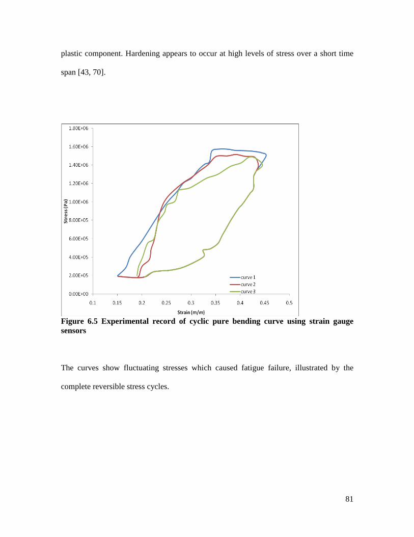
81

plastic component. Hardening appears to occur at high levels of stress over a short time

span [43, 70].

Figure 6.5 Experimental record of cyclic pure bending curve using strain gauge sensors

The curves show fluctuating stresses which caused fatigue failure, illustrated by the

complete reversible stress cycles.

82

Figure 6.6 Cyclic loading for pure bending curve using piezoelectric sensor

Next, the experiments were manipulated to focus on a single cycle by taking the mean

value per cycle as illustrated in Fig. 6.7 and Fig. 6.8, considering the mid-life of the

hysteresis loop [83].

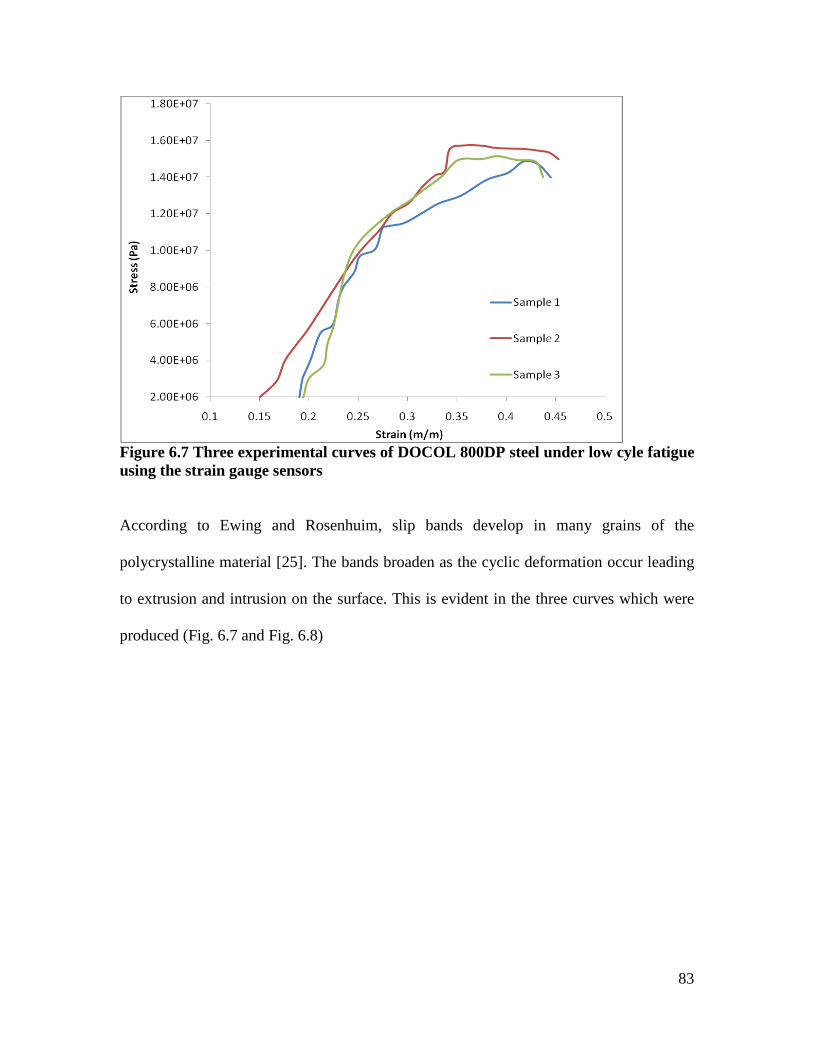
83

Figure 6.7 Three experimental curves of DOCOL 800DP steel under low cyle fatigue using the strain gauge sensors

According to Ewing and Rosenhuim, slip bands develop in many grains of the

polycrystalline material [25]. The bands broaden as the cyclic deformation occur leading

to extrusion and intrusion on the surface. This is evident in the three curves which were

produced (Fig. 6.7 and Fig. 6.8)

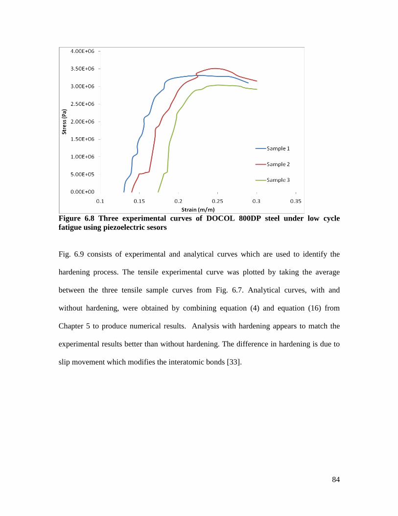
84

Figure 6.8 Three experimental curves of DOCOL 800DP steel under low cycle fatigue using piezoelectric sesors

Fig. 6.9 consists of experimental and analytical curves which are used to identify the

hardening process. The tensile experimental curve was plotted by taking the average

between the three tensile sample curves from Fig. 6.7. Analytical curves, with and

without hardening, were obtained by combining equation (4) and equation (16) from

Chapter 5 to produce numerical results. Analysis with hardening appears to match the

experimental results better than without hardening. The difference in hardening is due to

slip movement which modifies the interatomic bonds [33].

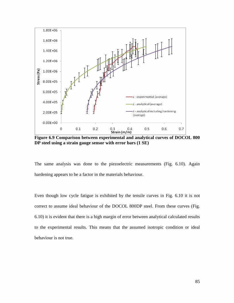
85

Figure 6.9 Comparison between experimental and analytical curves of DOCOL 800 DP steel using a strain gauge sensor with error bars (1 SE) The same analysis was done to the piezoelectric measurements (Fig. 6.10). Again

hardening appears to be a factor in the materials behaviour.

Even though low cycle fatigue is exhibited by the tensile curves in Fig. 6.10 it is not

correct to assume ideal behaviour of the DOCOL 800DP steel. From these curves (Fig.

6.10) it is evident that there is a high margin of error between analytical calculated results

to the experimental results. This means that the assumed isotropic condition or ideal

behaviour is not true.

86

Figure 6.10 Comparison between the analytical curve and experimental curve of piezoelectric sensor with standard error bars (1 SE)

It can be concluded that both strain measuring instruments recorded similar material

behaviour but at different stresses. This means that the specimen experienced strain

hardening and thus oσ - hardening effect (Fig. 6.9 and Fig. 6.10) plays a factor in the

materials behaviour.

The two experimental curves using the strain gauge and the piezoelectric sensor are

compared against each other in Fig. 6.11. Initially the strain gauge and the piezoelectric

sensor behaved in similar manner until it reached stress levels above 0.5(MPa). The

curves show elastic behaviour shown by the straight line which resembles a stress-strain

relationship in an initial linear region. With the continued increase in stresses beyond the

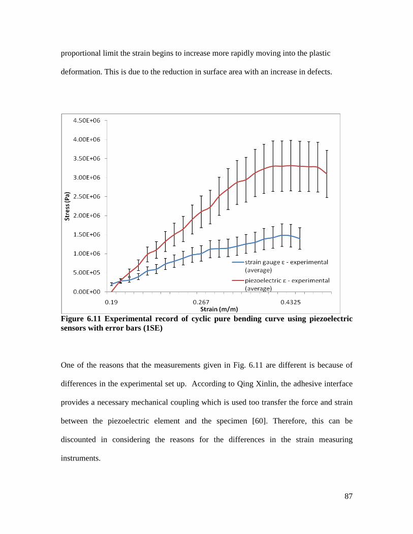
87

proportional limit the strain begins to increase more rapidly moving into the plastic

deformation. This is due to the reduction in surface area with an increase in defects.

Figure 6.11 Experimental record of cyclic pure bending curve using piezoelectric sensors with error bars (1SE)

One of the reasons that the measurements given in Fig. 6.11 are different is because of

differences in the experimental set up. According to Qing Xinlin, the adhesive interface

provides a necessary mechanical coupling which is used too transfer the force and strain

between the piezoelectric element and the specimen [60]. Therefore, this can be

discounted in considering the reasons for the differences in the strain measuring

instruments.

88

The results from the strain gauge sensor measured a far greater hardening in the material.

Testing often requires fairly precise measurement, and the resistance strain gauge is used

for its accuracy and precision because it can measure strains greater than several

percentage needed [14, 20]. Even though extensometers are customary used in

measuring low cycle fatigue; it can cause premature fracture on the material at the contact

point [44]. Therefore, the behaviour of the steel under the strain gauge measurement is

taken as the standard behaviour under cyclic loading.

In order to analyse the piezoelectric strain curves according to the standard behaviour the

results had to be adjusted using the analytical results (equations (4) and (16) from

Chapter 5). The piezoelectric sensor measurements are adjusted by dividing the stress

( ijσ ) with a factor of 2 and increasing the strain ( ijε ) by a factor of 0.1 (m/m). These

factors were derived from the difference between the analytical solutions for the strain

gauge and piezoelectric sensor. Fig. 6.12 gives a comparison of the strain measurements

using the strain gauge as before but with the new piezoelectric sensor curves.

89

Figure 6.12 Strain data measured with a strain gauge sensor compared to measured with a piezoelectric sensor but converted by the difference in analytical solutions (1SE)

Fig. 6.13 was generated by plotting the adjusted analytical curve for the piezoelectric

sensor against the experimental curve for the strain gauge; Fig. 6.14 shows the two

analytical curves for the piezoelectric sensor and the strain gauge sensor. It can be seen

that with factoring in errors, that the piezoelectric and strain gauge curves are more

compatible. The implication of these results goes further to substantiate that piezoelectric

sensor can be used in monitoring continuum damage in structures.

90

Figure 6.13 Adjusted analytical curve for the piezoelectric sensor against the experimental curve for the strain gauge (1SE)

Figure 6.14 The adjusted analytical curves for the piezoelectric sensor is compared with the analytical results for the strain gauge sensor (1SE) But, there are some critical differences between the two strain sensors which can be

mentioned.

91

The background noise from a resistive strain gauge, with its attendant bridge, amplifier,

and chart recorder, is electrical in origin, whilst the acoustic noise is much smaller. But

with a piezoelectric sensor, amplifier and chart recorder, the acoustic sensitivity is so

high that the background noise is dominated by acoustic rather than electrical

contributions. On these grounds the piezoelectric sensor is superior (see Fig. 6.12) to the

resistive strain gauge for the detection of paranormal metal bending signals. The

resistance of the piezoelectric material is almost infinitely high, so that the charge does

not leak away, and can be taken to be approximately proportional to the stress. It might

be measured on an electrometer amplifier, whose resistance is also almost infinitely high.

With this conversion there is a better fit between the two measuring devices (Fig. 6.13

and Fig. 6.14). Any further differences are likely to be due to other factors which are

explored further in the next chapter.

CONCLUSION

For the uni-axial system, tensile curves were plotted and analysed using classical

methods as described in Chapter 5. This investigation produced a standard tensile curve

which was used as a guide and also produced the material property for the structure.

Cyclic curves for the two strain sensors (strain gauge and piezoelectric) were plotted

from the cyclic test. Experimental and analytical analyses were carried out to determine if

92

a piezoelectric sensor can monitor degradation as well as a strain gauge (Fig. 6.12, Fig.

6.13 and Fig. 6.14).

The outcomes of the results show that piezoelectric sensor can be used to measure fatigue

failure on a ductile material.

93

Chapter 7

CONCLUSION

This study investigated the use of a piezoelectric technique for monitoring structural

degradation. Due to its highly sensitive to strain, piezoelectric sensors can be used as a

dynamic strain sensor [21].

The uni-axial loading, an experimental and numerical study of the mechanical behaviour

of DOCOL 800 DP steel specimen during conventional tensile test was carried out. An

elastic model was obtained by means of Hooke’s Law which uses the assumption that

each element of the body is in a state of static equilibrium. Elasticity and plasticity

equations, using Prandtl-Reuss were derived for further theoretical analysis. They were

used to produce analytical solutions so as to simulate the experimental stress-strain

curves. The results in this study show that a linear approximation of the uni-axially

loaded curves can be simplified analytically using Prandtl-Reuss [16].

94

Damage effects are coupled with elastic and plastic effects together form damage models

which were used. These models were used to understand the extent to which the

empirical behaviour of the material can be explained by damage models.

Cyclic monitoring of metal specimens using the two different signal sensors (strain gauge

and piezoelectric) under low cycle fatigue were carried out. The strain gauge was

soldered to an insulated wire consisting of a negative and positive wire. The wires were

connected directly to the bridge circuit. The Wheatstone Bridge Circuit comprised of

four resistors. The output of the strain gauge was then measured across the bridge circuit

as a voltage output [29].

The piezoelectric sensor was carefully glued to a rectangular plate to create a smart

structure, which underwent fatigue testing. The smart structure was used to monitor the

change in displacement caused by the external loading applied by the fatigue testing

machine. The displacement was represented by a voltage change across the piezoelectric

material [58].

In this study a piezoelectric sensor was shown to give similar results to a strain gauge

sensor. Differences are attributed to the background noise associated with the two

devices. The strain gauge showed it suffered more from noise interference (Fig. 6.12) as

compared to the piezoelectric sensor during testing. This is a critical difference between

95

the two strain sensors which shows that piezoelectric can be used as dynamic strain

sensor [21].

Therefore, a benefit of a self-monitoring structure is that it will reduce abrupt component

failure of the material under high to cyclic straining or stressing, like in turbine blades

[46].

It is currently understood that catastrophic or sudden failure of structures should be

dramatically reduced by using a self-monitoring structure for fatigue behaviour. One

possibility is the use of piezoelectric material for sensing behavioural change. This meant

that no signal conditioning was required to produce results due to the voltage induced on

the piezoelectric sensor. With this type of knowledge, industries will be able to use

piezoelectric sensors to daily monitor their operations and their structures under fatigue.

This system can also be used in vibration control of machinery under vigorous

operations.

This research study further supports theoretical knowledge about piezoelectric

techniques. Previous theoretical analysis largely focused on vibration control and current

induced loading. This investigation considered the mechanical testing (fatigue testing) of

structures using piezoelectric techniques. Further studies are needed to make the methods

of practical useful for industry. For example, to further improve the piezoelectric

capabilities new creep investigations must be carried out.

96

BIBLIOGRAPHY

1. Annual Book of ASTM Standard, Metals Test Methods and Analytical

Procedures, Volume 03.01, 2003.

2. Bayoumit. M. R., El Latif. K. A. Characterization of cyclic plastic bending of

austenitic aisi 304 stainless steel, Engineering Fracture Mechanics, 51, pp. 1049-

1058, 1995.

3. Benallal. A., Billardon. R., Lemaitre. J. Continuum damage mechanics and local

approach to fracture: Numerical procedures, Computer Methods in Applied

Mechanics and Engineering, 92, pp. 141-155, 1991.

4. Boresi. A. P., Schmidt. R.T., Sidebottom. O.R., Advanced Mechanics of Material,

4th Ed. pub: John Wiley and Son Inc, 1985.

5. Casas-Rodriguez. J. P., Ashcroft. I. A., Silberschmidt. V.V., Damage evolution in

adhesive joints subjected to impact fatigue, Journal of Sound and Vibration, 308,

pp. 467–478, 2007.

6. Chakrabarty. J. Theory of plasticity, pub: McGraw Hill Company, 1987.

7. Chan. T.N.T., Li. Z. X. Fatigue analysis and life prediction of bridges with

structural health monitoring data- Part II application, International Journal of

Fatigue, 23, pp. 55-64, 2001.

8. Chandrakanth. S. Damage couple elasto-plastic finite element analysis of a

Timoshenko layered beam, Computer and Structures, 69, pp. 411-420, 1998.

9. Chen. W. Q., Lim. C. W., Ding. H. J. Point temperature solution for a penny-

shaped crack in an infinite transversely isotropic thermo-piezo-elastic,

97

Engineering Analysis with Boundary Elements, 29, pp. 524-532, 2005.

10. Cody. W. Piezoelectric, pub: McGraw-Hill, 1964.

11. Collins. J. A. Failure of Materials in Mechanical Design, pub: John Wiley & Son,

2nd Ed, 1993.

12. Daunys. M., Rimovskis. S. Analysis of circular cross-section element, loaded by

static and cyclic elastic-plastic pure bending, International Journal of Fatigue, 28,

pp. 211-222, 2006.

13. Davis. H.E., Troxell. G.E., Wiskoul. C.T. The testing and inspection of

engineering materials, pub: McGraw-Hill, 2nd Ed, 1955.

14. Davis. H.E., Troxell. G.E., Wiskoul. C.T. The testing of Engineering Materials,

pub: McGraw-Hill, 4th Ed, 1964.

15. Detwiler. D.T., Shen. M. H. H., Venkayya. V. B., finite element analysis of

laminated composite structure containing distributed piezoelectric actuator and

sensor, Finite Element in Analysis and Design, 20, pp. 87-100, 1995.

16. Dieter. G. E. Mechanical Metallurgy, pub: McGraw Hill Company, SI metric Ed,

1988.

17. Docol UHS- Cold Reduced Ultra Strength Steel.

18. Dowling. N.E. Mechanical behaviour of materials: engineering methods for

deformation, fracture, and fatigue, pub: Prentice Hall, 2nd Ed, 1999.

19. Eduardo. E.C., Diego. J.C. 2003. Experimental and numerical analysis of the

tensile test using sheet specimens. Finite Elements in Analysis and Design, 40, pp.

555-575, 2004.

20. Fenner. A.J. Mechanical Testing of Materials, pub: Newnes, 1965.

98

21. Gama. A. L., Morikawa. S. R. K., Monitoring Fatigue Crack Growth in Compact

Tension Specimens Using Piezoelectric Sensors, Society for Experimental

Mechanics, 48 pp. 247–252, 2007.

22. Goyal. S., Sandhya. R., Valsan M., Bhanu. K., Rao. S., The effect of thermal

ageing on low cycle fatigue behaviour of 316 stainless steel welds, International

Journal of Fatigue, 31, pp. 447–454, 2009.

23. Grosse. M. Monitoring of low-cycle fatigue degradation in X6CrNiTi18-10

austenitic steel, Journal of Nuclear Material, 296, pp. 305 -311, 2001.

24. Heino. S., Karlsson. B. Cyclic deformation and fatigue behaviour of 7mo–0.5n

superaustenitic stainless steel—stress–strain relations and fatigue life, Acta Mater.

49, pp. 339–351, 2001.

25. History of fatigue. [Online] available: http://en.wikipedia.org/wiki/Metal_fatigue,

[accessed 20 May 2006].

26. History of Piezoelectrics [Online] available: http://www.piezo.com, [accessed 12

March 2006].

27. History of Steel [online]. 2004. Available: http://college.hmco/history [Accessed

12 February 2006].

28. History of strain gauge [online]. 1998. Available: http://www.omega.com

[Accessed on 20 February 2006].

29. How does strain gauge operate [online]. 1998. Available:

http://www.sensorland.com [Accessed 06 March 2006].

99

30. Hwang. W. S., Park. H. G., Finite element modeling of piezoelectric sensor and

actuator, AAIA Journal, 31, pp. 930-937, 1993.

31. Instron: Material Testing Machines for Tensile, Fatigue, Impact, Structural

Hardness, Fatigue Testing Materials [online]. 2004. Available:

http://www.instron.com [Accessed 12 February 2006].

32. Iron [online]. 2004. Available: http://www.appaltree.net /aba/iron.html [Accessed

14 February 2006].

33. Kachanov, L. M. Introduction to continuum damage mechanics, pub: Nijhoff, 2nd

Ed, 1986.

34. Kanchanomai. C., Yamamoto. S., Miyashita. Y. Low cycle fatigue test for solders

using non-contact digital image measurement system, International Journal of

Fatigue, 24, pp. 57–67, 2002.

35. Kandil. F.A. Potential ambiguity in determination of plastic strain range

component in LCF testing, International Journal of Fatigue, 21, pp. 1013-1018,

1999.

36. Kekana M. A static shape control model for piezo-elastic composite structure,

Composite structures, 59, pp. 129-135, 2003.

37. Kekana. M. An improved finite element model for vibration and control

simulation of smart composite structures with embedded piezoelectric sensor and

actuator, D.Tech thesis, Technikon Natal, Durban 2001.

38. Kekana. M. Finite Element Modelling of Laminated Piezo-Elastic Structures:

LYAPUNOV STABILITY ANALYSIS, Journal of Sound and Vibration, 256,

pp. 463-473, 2002.

100

39. Kekana. M., Badur. J. An analysis of piezo-elastic restrictor using a capacitive

shunt, Task Quarterly, 8, pp. 377-384, 2004.

40. Kekana. M., Badur. J. Modelling of Beams using the reduced integration

technique: static and free vibration, R&D Journal, 16, pp. 9-15, 2000.

41. Kekana. M., Tabakov. P. Static control of composite plates using piezoelectric

sensor and actuator techniques, Smart Material and Structures, 14, pp. 349-353,

2005.

42. Kekana. M., Tabakov. P., Walker. M. A shape control model for piezo-electric

structures based on divergence free electric displacement, International Journal of

Solid and Structures, 40, pp. 715-727, 2003.

43. Klensil. M., Lukas. P. Fatigue of Metallic materials, pub: Elsevier, 2nd Ed, 1992.

44. Kramberger. J. Numerical calculation of bending fatigue life of thin-rim spur

gear, Engineering Fracture Mechanics, 71, pp. 647-656, 2004.

45. Kubota. M., Kataoka. S.,Kondo.Y., Effect of stress relief groove on fretting

fatigue strength and index for the selection of optimal groove shape, International

Journal of Fatigue, 31, pp. 439–446, 2009.

46. Kumar. S., Niranjan. R., Ganguli, R. Monitoring low cycle fatigue damage in

turbine blade using vibration characteristics, Mechanical Systems and Signal

Processing.

47. Lemaitre. J. Coupled elasto-plasticity and damage constitutive equations,

Computer Methods in Applied Mechanics and Engineering, 51, pp. 31-49, 1985.

48. Lemaitre. J. How to use damage mechanics, Nuclear Engineering and

Design, 80, pp. 233-245, 1984.

101

49. Lemaitre. J., Dufailly. J. Damage measurements, Engineering Fracture

Mechanics, 28, pp. 643-661, 1987.

50. Li. B., Reis. M., de Freitas. M. Simulation of cyclic stress/strain evolutions for

multiaxial fatigue life prediction, International Journal of Fatigue, 28, pp. 451-

458, 2006.

51. Mahmoodia. S. N., Jalilia. N., Khademb. S. E, An experimental investigation of

nonlinear vibration and frequency response analysis of cantilever viscoelastic

beams, Journal of Sound and Vibration, 311, pp. 1409–1419, 2008.

52. Malésys. N., Vincent. L., Hild. F., A probabilistic model to predict the formation

and propagation of crack networks in thermal fatigue, International Journal of

Fatigue,31, pp. 565–574, 2009.

53. Mentes. G., Eper-Pupai. I. Investigation of meteorological effects on strain

measurements at two stations in hungry, Journal of Geodymanics, 41, pp. 259-

267, 2006.

54. Miller. S. E. Active distributed vibration control of anisotropic piezoelectric

laminated plate, Journal of Sound and Vibration, 183, pp. 797-817, 1995.

55. MTS Systems Corporation: Testing Systems, Sensor Solution, and Simulation

System [online]. 2004. Available: http://www.mts.com [Accessed 12 February

2006].

56. Park. S-J., Park. S-P. Failure and damage of steel thin plate elements and angle

members due to very low-cycle loading, Engineering Structures, 20, pp. 1623-

1632, 2004.

57. Patankar. R., Ray. A. State-space modelling of fatigue crack growth in ductile

102

alloy, Engineering Fracture Mechanics, 66, pp. 129-151, 2000.

58. Piezoelectric sensor [online]. 2005. Available:

http://en.wikipeadia.org/wiki/piezoelectric_sensor [Accessed 04 January 2008].

59. Pirondi. A., Bonors. N., Steglich. D., Brocks. W., Hellman. D. Simulation of

failure under cyclic plastic loading by damage models, International Journal of

Plasticity, 22, pp. 2146-2170, 2006.

60. Qing. Xinlin. P. Effect of adhesive on the performance of piezoelectric elements

used to monitor structural health, International Journal of Adhesion and Adhesive,

26, pp. 622-628, 2006.

61. Rankine. W. J. M. On the causes of unexpected breakage of the journal of railway

axles and the means of preventing such accidents by observing the law of

continuity in their construction, Proceeding of the institute of civil engineers, pp.

105-108.

62. Read. D. T. Tension-tension fatigue of copper thin film, International Journal of

Fatigue, 20, pp. 203-209, 1998.

63. Sagar. S.P. Magnetic Barkhausen emission evaluate fatigue damage in low carbon

structural steel, International Journal of Fatigue, 27, pp. 317-322, 2005.

64. Sánchez-Santana. U., Rubio-González. C., Mesmacque. G., Amrouche. A.,

Decoopman. X., Effect of fatigue damage induced by cyclic plasticity on the

dynamic tensile behavior of materials, International Journal of Fatigue, 30, pp.

1708–1719, 2008.

65. Scruggs. J.T., An optimal stochastic control theory for distributed energy

harvesting networks, Journal of Sound and Vibration

103

66. Shames. I. H. Introduction to Solid Mechanics, pub: Prentice Hall, 2nd Ed, 1975.

67. Smith. W.F. Foundation of Material Science and Engineering. 2nd Ed.

68. Srinivasan. V. S., Sandhya. R. Comparative evaluation of strain controlled low

cycle fatigue behaviour of solution annealed and prior cold worked 316L (N)

stainless steel, International Journal of Fatigue, 26, pp. 1295–1302, 2004.

69. Srinivasan. V. S., Valsan. M. High temperature time-dependent low cycle fatigue

behaviour of a type 316L (N) stainless steel, International Journal of Fatigue, 21,

pp. 11–21, 1999.

70. Suresh. S. Fatigue of materials, pub: University of Cambridge, 1st pbk Ed, 1992.

71. Surowiak. Z. Influence of cyclic phase transitions on some properties of the

ferroelectric perovskites, Journal of European Ceramic Society, 22, pp. 1863-

1866, 2002.

72. Tensile Testing [online]. 1998. Available: http://www.mech.com [Accessed on 10

March 2006].

73. The Strain Gauge: Omega [online]. Available:

http://www.omega.com/LiteratureTransactions/Volume3/strain [Accessed 20

February 2006].

74. Thomas. J., Abbas. B.A.H. Finite element model for dynamic analysis of

Timoshenko beam, Journal of Sound and Vibration, 4, pp. 291-299, 1975.

75. Timoshenko. S.P. History of Strength of Material, pub: McGraw-Hill Company,

2nd Ed.

76. Tzou H.S., Chai. W.K. Design and testing of a hybrid polymeric electrostrictive/

piezoelectric beam with bang-bang control, Mechanical System and Signal

104

Processing.

77. Tzou. H. S., Tseng. C. I. Distributed piezoelectric sensor/actuator design for

dynamic measurement/control of distributed parameter systems: A piezoelectric

finite element approach, Journal of Sound and Vibration, 138, pp. 17-34, 1990.

78. Tzou. H.S., Gache. Theoretical analysis of a multilayered thin shell coupled with

piezoelectric shell actuator for distributed vibration control, Journal of Sound and

Vibration, 132, pp. 433-450, 1989.

79. Wang. B., Vibration analysis of a continuous system subject to generic forms of

actuation forces and sensing devices, Journal of Sound and Vibration, 297, pp.

680–693, 2006.

80. Wang. R., Shang D., Low-cycle fatigue life prediction of spot welds based on

hardness distribution and finite element analysis, International Journal of

Fatigue,31, pp. 508–514 , 2009.

81. Xing-Jian Dong, Guang Meng, Juan-Chun Peng, Vibration control of

piezoelectric smart structures based on system identification technique: Numerical

simulation and experimental study, Journal of Sound and Vibration, 297, pp.

680–693, 2006.

82. Yana.W., Limc C.W., Chena. W.Q., Caia J.B., A coupled approach for damage

detection of framed structures using piezoelectric signature, Journal of Sound and

Vibration, 307, pp. 802–817, 2007.

83. Yoon. S., Hong. S., Lee, S., Kim. B. Low cycle fatigue testing of 429EM stainless

steel pipe, International Journal of Fatigue, 25, pp. 1301-1307, 2003.