use of plasma actuators as a moving-wake generator · use of plasma actuators as a moving ......
TRANSCRIPT

Thomas C. Corke, Flint O. Thomas, and Michael J. Klapetzky
University of Notre Dame, Notre Dame, Indiana
Use of Plasma Actuators as a Moving-WakeGenerator
NASA/CR—2007-214676
January 2007
https://ntrs.nasa.gov/search.jsp?R=20070010028 2018-06-19T09:03:14+00:00Z

NASA STI Program . . . in Profile
Since its founding, NASA has been dedicated to the
advancement of aeronautics and space science. The
NASA Scientific and Technical Information (STI)
program plays a key part in helping NASA maintain
this important role.
The NASA STI Program operates under the auspices
of the Agency Chief Information Officer. It collects,
organizes, provides for archiving, and disseminates
NASA’s STI. The NASA STI program provides access
to the NASA Aeronautics and Space Database and its
public interface, the NASA Technical Reports Server,
thus providing one of the largest collections of
aeronautical and space science STI in the world.
Results are published in both non-NASA channels and
by NASA in the NASA STI Report Series, which
includes the following report types:
• TECHNICAL PUBLICATION. Reports of
completed research or a major significant phase
of research that present the results of NASA
programs and include extensive data or theoretical
analysis. Includes compilations of significant
scientific and technical data and information
deemed to be of continuing reference value.
NASA counterpart of peer-reviewed formal
professional papers but has less stringent
limitations on manuscript length and extent of
graphic presentations.
• TECHNICAL MEMORANDUM. Scientific
and technical findings that are preliminary or
of specialized interest, e.g., quick release
reports, working papers, and bibliographies that
contain minimal annotation. Does not contain
extensive analysis.
• CONTRACTOR REPORT. Scientific and
technical findings by NASA-sponsored
contractors and grantees.
• CONFERENCE PUBLICATION. Collected
papers from scientific and technical
conferences, symposia, seminars, or other
meetings sponsored or cosponsored by NASA.
• SPECIAL PUBLICATION. Scientific,
technical, or historical information from
NASA programs, projects, and missions, often
concerned with subjects having substantial
public interest.
• TECHNICAL TRANSLATION. English-
language translations of foreign scientific and
technical material pertinent to NASA’s mission.
Specialized services also include creating custom
thesauri, building customized databases, organizing
and publishing research results.
For more information about the NASA STI
program, see the following:
• Access the NASA STI program home page at
http://www.sti.nasa.gov
• E-mail your question via the Internet to
• Fax your question to the NASA STI Help Desk
at 301–621–0134
• Telephone the NASA STI Help Desk at
301–621–0390
• Write to:
NASA Center for AeroSpace Information (CASI)
7115 Standard Drive
Hanover, MD 21076–1320

Use of Plasma Actuators as a Moving-WakeGenerator
NASA/CR—2007-214676
January 2007
National Aeronautics and
Space Administration
Glenn Research Center
Cleveland, Ohio 44135
Prepared under Cooperative Agreement NCC3–935
Thomas C. Corke, Flint O. Thomas, and Michael J. Klapetzky
University of Notre Dame, Notre Dame, Indiana

Acknowledgments
The authors gratefully acknowledge the valuable help and advice of the technical monitor Dr. David Ashpis and the funding
from NASA Glenn Research Center that made this work possible.
Available from
NASA Center for Aerospace Information
7115 Standard Drive
Hanover, MD 21076–1320
National Technical Information Service
5285 Port Royal Road
Springfield, VA 22161
Available electronically at http://gltrs.grc.nasa.gov
Trade names and trademarks are used in this report for identification
only. Their usage does not constitute an official endorsement,
either expressed or implied, by the National Aeronautics and
Space Administration.
This work was sponsored by the Fundamental Aeronautics Program
at the NASA Glenn Research Center.
Level of Review: This material has been technically reviewed by NASA technical management.
Executive Summary
The work documented in this report tests the concept of using plasma actuators as a simple and easy
way to generate a simulated moving-wake and the disturbances associated with it in turbines. This wake is
caused by the blades of the upstream stages of the turbine. Two types of devices, one constructed of arrays
of NACA 0018 airfoils, and the one constructed of flat plates were studied. The airfoils or plates were
equipped with surface mounted dielectric barrier discharge (DBD) plasma actuators, which were used to
generate flow disturbances resembling moving-wakes. CTA hot-wire anemometry and flow visualization
using a smoke-wire were used to investigate the wake independence at various spacings and downstream
locations. The flat plates were found to produce better results than the airfoils in creating large velocity
fluctuations in the free-stream flow. Different dielectric materials, plasma actuator locations, leading edge
contours, angles of attack and plate spacings were investigated, some with positive results. The magnitudes
of the velocity fluctuations were found to be comparable to existing mechanical moving-wake generators,
thus proving the feasibility of using plasma actuators as a moving-wake generator.
NASA/CR—2007-214676 iii


CONTENTS
LIST OF FIGURES . . . . . . . . . . . . . . . . . . . . . . . . . . . . . . . .
LIST OF TABLES . . . . . . . . . . . . . . . . . . . . . . . . . . . . . . . . .
LIST OF SYMBOLS . . . . . . . . . . . . . . . . . . . . . . . . . . . . . . . .
CHAPTER 1: INTRODUCTION . . . . . . . . . . . . . . . . . . . . . . . . . 11.1 Motivation . . . . . . . . . . . . . . . . . . . . . . . . . . . . . . . . . 11.2 Background . . . . . . . . . . . . . . . . . . . . . . . . . . . . . . . . 41.3 Objectives . . . . . . . . . . . . . . . . . . . . . . . . . . . . . . . . . 9
CHAPTER 2: EXPERIMENTAL SETUP . . . . . . . . . . . . . . . . . . . . 102.1 Wind Tunnel . . . . . . . . . . . . . . . . . . . . . . . . . . . . . . . 102.2 Traverse . . . . . . . . . . . . . . . . . . . . . . . . . . . . . . . . . . 182.3 Data Acquisition . . . . . . . . . . . . . . . . . . . . . . . . . . . . . 202.4 Plasma Actuators . . . . . . . . . . . . . . . . . . . . . . . . . . . . . 242.5 Test and Actuator Configurations . . . . . . . . . . . . . . . . . . . . 26
2.5.1 Configuration 1 . . . . . . . . . . . . . . . . . . . . . . . . . . 282.5.2 Configuration 2 . . . . . . . . . . . . . . . . . . . . . . . . . . 302.5.3 Configuration 3 . . . . . . . . . . . . . . . . . . . . . . . . . . 322.5.4 Configuration 4 . . . . . . . . . . . . . . . . . . . . . . . . . . 342.5.5 Configuration 5 . . . . . . . . . . . . . . . . . . . . . . . . . . 352.5.6 Configuration 6 . . . . . . . . . . . . . . . . . . . . . . . . . . 36
2.6 Flow Visualization . . . . . . . . . . . . . . . . . . . . . . . . . . . . 382.7 Data Reduction . . . . . . . . . . . . . . . . . . . . . . . . . . . . . . 42
CHAPTER 3: RESULTS: AIRFOIL . . . . . . . . . . . . . . . . . . . . . . . 473.1 Single Airfoil . . . . . . . . . . . . . . . . . . . . . . . . . . . . . . . 47
3.1.1 Wake Profiles . . . . . . . . . . . . . . . . . . . . . . . . . . . 483.1.2 Similarity Plot . . . . . . . . . . . . . . . . . . . . . . . . . . 49
3.2 Twin Airfoils . . . . . . . . . . . . . . . . . . . . . . . . . . . . . . . 523.2.1 Wake Profiles . . . . . . . . . . . . . . . . . . . . . . . . . . . 52
NASA/CR—2007-214676 v
vii
xi
xiii
3.2.2 Similarity Plots . . . . . . . . . . . . . . . . . . . . . . . . . . 623.3 Comparison: Single Airfoil to Twin Airfoils . . . . . . . . . . . . . . . 633.4 Flow Visualization . . . . . . . . . . . . . . . . . . . . . . . . . . . . 68
CHAPTER 4: RESULTS: FLAT PLATES . . . . . . . . . . . . . . . . . . . . 744.1 Configuration 2 . . . . . . . . . . . . . . . . . . . . . . . . . . . . . . 74
4.1.1 Zero Angle of Attack . . . . . . . . . . . . . . . . . . . . . . . 754.1.2 At Angle of Attack . . . . . . . . . . . . . . . . . . . . . . . . 78
4.2 Configuration 3 . . . . . . . . . . . . . . . . . . . . . . . . . . . . . . 824.2.1 Flow Visualization . . . . . . . . . . . . . . . . . . . . . . . . 824.2.2 Hot-Wire Measurements . . . . . . . . . . . . . . . . . . . . . 86
4.3 Configuration 4 . . . . . . . . . . . . . . . . . . . . . . . . . . . . . . 944.3.1 0 Degree Angle of Attack . . . . . . . . . . . . . . . . . . . . . 97
4.4 Comparison: Configuration 3 and 4 To Single Plate . . . . . . . . . . 101
CHAPTER 5: RESULTS: UNIFORM FLAT PLATES . . . . . . . . . . . . . 1095.1 Configuration 5 . . . . . . . . . . . . . . . . . . . . . . . . . . . . . . 109
5.1.1 Comparison: Configuration 5 To Single Plate . . . . . . . . . 1145.1.2 Actuator Phasing . . . . . . . . . . . . . . . . . . . . . . . . . 117
5.2 Configuration 6 . . . . . . . . . . . . . . . . . . . . . . . . . . . . . . 1205.2.1 Forcing Upstream . . . . . . . . . . . . . . . . . . . . . . . . . 1215.2.2 Forcing Downstream . . . . . . . . . . . . . . . . . . . . . . . 1265.2.3 Comparison: Upstream to Downstream Forcing . . . . . . . . 131
CHAPTER 6: RESULTS: DISCUSSION . . . . . . . . . . . . . . . . . . . . . 1346.1 Leading Edge Dependence . . . . . . . . . . . . . . . . . . . . . . . . 1346.2 Actuator Effect: At 5 Chord Lengths Downstream . . . . . . . . . . . 1376.3 Actuator Effect: At Other Chord Lengths Downstream . . . . . . . . 142
CHAPTER 7: CONCLUSIONS AND RECOMMENDATIONS . . . . . . . . . 1477.1 Conclusions . . . . . . . . . . . . . . . . . . . . . . . . . . . . . . . . 1477.2 Recommendations for Future Work . . . . . . . . . . . . . . . . . . . 151
REFERENCES . . . . . . . . . . . . . . . . . . . . . . . . . . . . . . . . . . . i
NASA/CR—2007-214676 vi

LIST OF FIGURES
1.1 Illustration of concept of the moving-wake generator. . . . . . . . . . . . 41.2 Schematic of the rotating bar wake generator used by Doorly. [7] . . . . . 51.3 Additional examples of cylinder setups. . . . . . . . . . . . . . . . . . . 71.4 Principle of Dibelius and Ahlers wake generator. [5] . . . . . . . . . . . . 8
2.1 Wind tunnel fan before final assembly. . . . . . . . . . . . . . . . . . . . 122.2 The screen boxes before final assembly. . . . . . . . . . . . . . . . . . . 132.3 The contraction during construction. . . . . . . . . . . . . . . . . . . . . 152.4 Flow turning section during construction. . . . . . . . . . . . . . . . . . 162.5 The fully completed wind tunnel. . . . . . . . . . . . . . . . . . . . . . 172.6 The spanwise traversing system. . . . . . . . . . . . . . . . . . . . . . . 192.7 Circuit diagram of the gain circuit used. . . . . . . . . . . . . . . . . . . 212.8 Circuit diagram of the filter circuit used. . . . . . . . . . . . . . . . . . . 222.9 Flow chart of data acquisition setup. . . . . . . . . . . . . . . . . . . . . 232.10 Illustration of a plasma actuator. . . . . . . . . . . . . . . . . . . . . . . 262.11 The various test specimen holders used. . . . . . . . . . . . . . . . . . . 292.12 Example of single and dual airfoil setups. . . . . . . . . . . . . . . . . . 292.13 Airfoil with Kapton actuator at leading edge and template. . . . . . . . . 312.14 A sketch of an overhead view of the experimental test setup. . . . . . . . 312.15 Configuration 2, Kapton actuator flat plate setup. . . . . . . . . . . . . . 322.16 Configuration 3, setup for flat plate with PC type actuator. . . . . . . . . 342.17 Configuration 4, setup for flat plate with PC type actuator. . . . . . . . . 342.18 Configuration 5, setup for flat plate with PC type actuator. . . . . . . . . 352.19 Configuration 6, sandwich type actuator setup. . . . . . . . . . . . . . . 362.20 Image summary of the different configuration. . . . . . . . . . . . . . . . 372.21 ‘L’ shaped smoke-wire holder/fluid applicator. . . . . . . . . . . . . . . . 392.22 Flow visualization experimental setup. . . . . . . . . . . . . . . . . . . . 412.23 Examples of imaging effects from flow visualization setup. . . . . . . . . . 432.24 Air temperature dependence relative to time and free-stream velocity. t=0:60
for calibration(max. velocity 85 ft/s (25.9 m/s)), t=60:90 v=29 ft/s (8.84m/s), t=90:120 v=43 ft/s (13.1 m/s) . . . . . . . . . . . . . . . . . . . . 44
2.25 Select stream profiles of an actuator ‘off’ and ‘on’ case plotted with differencebetween them. A-Location minimum velocity of the actuator ‘off’ case. B-Indication of center of the plate area blockage. C-Represents the angle ofattack of the plate and projected area. . . . . . . . . . . . . . . . . . . . 46
3.1 Wake profile behind a single NACA 0018 airfoil, low Reynolds number case. 493.2 Corresponding RMS profile behind a single NACA 0018 airfoil, low Reynolds
number case. . . . . . . . . . . . . . . . . . . . . . . . . . . . . . . . . 50
NASA/CR—2007-214676 vii

3.3 Wake profile behind a single NACA 0018 airfoil, high Reynolds number case. 503.4 Corresponding RMS profile behind a single NACA 0018 airfoil, high Reynolds
number case. . . . . . . . . . . . . . . . . . . . . . . . . . . . . . . . . 513.5 Similarity plots for single airfoil. . . . . . . . . . . . . . . . . . . . . . . 523.6 Wake profiles behind two NACA 0018 airfoils at 1/3rd chord spacing, low
Reynolds number case. . . . . . . . . . . . . . . . . . . . . . . . . . . . 543.7 Corresponding RMS profiles behind two NACA 0018 airfoils at 1/3rd chord
spacing, low Reynolds number case. . . . . . . . . . . . . . . . . . . . . 543.8 Wake profiles behind two NACA 0018 airfoils at 2/3rd chord spacing, low
Reynolds number case. . . . . . . . . . . . . . . . . . . . . . . . . . . . 553.9 Corresponding RMS profiles behind two NACA 0018 airfoils at 2/3rd chord
spacing, low Reynolds number case. . . . . . . . . . . . . . . . . . . . . 563.10 Wake profiles behind two NACA 0018 airfoils at 1 chord spacing, low Reynolds
number case. . . . . . . . . . . . . . . . . . . . . . . . . . . . . . . . . 573.11 Corresponding RMS profiles behind two NACA 0018 airfoils at 1 chord spac-
ing, low Reynolds number case. . . . . . . . . . . . . . . . . . . . . . . 573.12 Wake profiles behind two NACA 0018 airfoils at 1/3rd chord spacing, high
Reynolds number case. . . . . . . . . . . . . . . . . . . . . . . . . . . . 583.13 Corresponding RMS profiles behind two NACA 0018 airfoils at 1/3rd chord
spacing, high Reynolds number case. . . . . . . . . . . . . . . . . . . . . 593.14 Wake profiles behind two NACA 0018 airfoils at 2/3rd chord spacing, high
Reynolds number case. . . . . . . . . . . . . . . . . . . . . . . . . . . . 603.15 Corresponding RMS profiles behind two NACA 0018 airfoils at 2/3rd chord
spacing, high Reynolds number case. . . . . . . . . . . . . . . . . . . . . 603.16 Wake profiles behind two NACA 0018 airfoils at 1 chord spacing, high
Reynolds number case. . . . . . . . . . . . . . . . . . . . . . . . . . . . 613.17 Corresponding RMS profiles behind two NACA 0018 airfoils at 1 chord spac-
ing, high Reynolds number case. . . . . . . . . . . . . . . . . . . . . . . 613.18 Centerline velocity decay for different spacings. . . . . . . . . . . . . . . 623.19 Similarity Plots at 1/3 chord Spacing. . . . . . . . . . . . . . . . . . . . 633.20 Similarity Plots at 2/3 chord Spacing. . . . . . . . . . . . . . . . . . . . 643.21 Similarity Plots at 1 chord Spacing. . . . . . . . . . . . . . . . . . . . . 643.22 Velocity decay for different spacings and single airfoil. . . . . . . . . . . . 653.23 RMS decay for different spacings and single airfoil. . . . . . . . . . . . . 663.24 Wake half-width decay for different spacings and single airfoil. . . . . . . 673.25 Flow visualization for non-actuated 1/3rd chord spacing case at 15.4 ft/s
(4.69 m/s). . . . . . . . . . . . . . . . . . . . . . . . . . . . . . . . . . 693.26 Flow visualization for non-actuated 2/3rd chord spacing case at 15.4 ft/s
(4.69 m/s). . . . . . . . . . . . . . . . . . . . . . . . . . . . . . . . . . 693.27 Flow visualization for non-actuated 1 chord spacing case at 15.4 ft/s (4.69
m/s). . . . . . . . . . . . . . . . . . . . . . . . . . . . . . . . . . . . . 703.28 Comparison with actuator at 25 percent chord, forward of the point of
maximum thickness of airfoil, at 6.3 KV potential. . . . . . . . . . . . . . 713.29 Comparison with actuator at 25 percent chord, forward of the point of
maximum thickness of airfoil, at 12.5 KV potential. . . . . . . . . . . . . 713.30 Comparison with actuator at 27 percent chord, point of maximum thickness
of airfoil, at 6.3 KV potential. . . . . . . . . . . . . . . . . . . . . . . . 72
NASA/CR—2007-214676 viii
3.31 Comparison with actuator at 27 percent chord, point of maximum thicknessof airfoil, 12.5 KV potential. . . . . . . . . . . . . . . . . . . . . . . . . 72
3.32 Comparison with actuator at 30 percent chord, behind the point of maxi-mum thickness of airfoil, 6.3 KV potential. . . . . . . . . . . . . . . . . . 73
3.33 Comparison with actuator at 30 percent chord, behind the point of maxi-mum thickness of airfoil, 12.5 KV potential. . . . . . . . . . . . . . . . . 73
4.1 Four actuators with 1/2 chord plate spacing at a maximum voltage potentialof 1.9 KV. . . . . . . . . . . . . . . . . . . . . . . . . . . . . . . . . . 76
4.2 Four actuators with 1/4 chord plate spacing at a maximum voltage potentialof 6.8 KV. . . . . . . . . . . . . . . . . . . . . . . . . . . . . . . . . . 77
4.3 One actuator at leading edge of plate at zero degrees, 11.2 KV voltagepotential, and 1 chord plate spacing. . . . . . . . . . . . . . . . . . . . . 79
4.4 One actuator at leading edge of plate at 5o, 11.2 KV voltage potential, and1 chord plate spacing. . . . . . . . . . . . . . . . . . . . . . . . . . . . 79
4.5 One actuator at leading edge of plate at 10o, 11.2 KV voltage potential, and1 chord plate spacing. . . . . . . . . . . . . . . . . . . . . . . . . . . . 80
4.6 One actuator at leading edge of plate 16o, 11.2 KV voltage potential and 1chord plate spacing. . . . . . . . . . . . . . . . . . . . . . . . . . . . . 80
4.7 −3o, 1 chord plate spacing, and 8.4 KV maximum voltage potential case. . 844.8 −5o, 1 chord plate spacing, and 8.4 KV maximum voltage potential case. . 844.9 −7o, 1 chord plate spacing, and 8.4 KV maximum voltage potential case. . 854.10 −3o, 1 chord plate spacing, and 11.2 KV maximum voltage potential case. 854.11 −5o, 1 chord plate spacing, and 11.2KV maximum voltage potential case. . 864.12 −7o, 1 chord plate spacing, and 11.2 KV maximum voltage potential case. 864.13 Stream profiles behind two flat plates at an angle of attack of −3o with a
plate spacing of 1 chord. . . . . . . . . . . . . . . . . . . . . . . . . . . 884.14 Stream profile behind two flat plates at an angle of attack of −3o with a
plate spacing of 1/2 chord. . . . . . . . . . . . . . . . . . . . . . . . . . 894.15 Similarity plot for two flat plates at an angle of attack of −3o with a plate
spacing of 1 chord and the actuator ‘off’. . . . . . . . . . . . . . . . . . 904.16 Similarity plot for two flat plates at an angle of attack of −3o with a plate
spacing of 1 chord and the actuator ‘on’. . . . . . . . . . . . . . . . . . . 914.17 Comparison of wake decay for the −3o angle of attack with 1 and 1/2 chord
plate spacings at 5.0 KHz frequency. . . . . . . . . . . . . . . . . . . . . 924.18 Comparison of wake decay for the −3o angle of attack with 1/2 chord plate
spacing at 5.0 KHz and 5.5 KHz frequencies. . . . . . . . . . . . . . . . 934.19 Power profile for 3 flat plates at an angle of attack of −3o and 1/2 chord
plate spacing. . . . . . . . . . . . . . . . . . . . . . . . . . . . . . . . . 954.20 Corresponding wake profiles from power study for 3 flat plates at an angle
of attack of −3o and 1/2 chord plate spacing. . . . . . . . . . . . . . . . 964.21 Power profile for 3 flat plates at an angle of attack of −3o and various plate
spacings. . . . . . . . . . . . . . . . . . . . . . . . . . . . . . . . . . . 974.22 Power profile for 3 flat plates at an angle of attack of 0o and 1/4 chord spacing. 984.23 Power profile for 3 flat plates at an angle of attack of 0o and various plate
spacings. . . . . . . . . . . . . . . . . . . . . . . . . . . . . . . . . . . 994.24 Summery of spacing effects at different applied voltage potentials. . . . . . 1004.25 Stream profiles behind 3 plates zero angle of attack. . . . . . . . . . . . . 101
NASA/CR—2007-214676 ix

4.26 Similarity plot for three flat plates at zero angle of attack with a 3/8 chordplate spacing and the actuator ‘off’. . . . . . . . . . . . . . . . . . . . . 102
4.27 Similarity plot for three flat plates at zero angle of attack with a 3/8 chordplate spacing and the actuator ‘on’. . . . . . . . . . . . . . . . . . . . . 102
4.28 Setup for single plate with 1/4 elliptic leading edge. . . . . . . . . . . . . 1034.29 Stream profiles behind single plate with 1/4 elliptic leading edge. . . . . . 1044.30 Comparison of stream profiles to single wake case with the 1/4 elliptic lead-
ing edge. . . . . . . . . . . . . . . . . . . . . . . . . . . . . . . . . . . 1054.31 Summary of actuator effect at the 5th chord location for all the stream and
power profiles thus far. . . . . . . . . . . . . . . . . . . . . . . . . . . . 108
5.1 Investigation of wake dependence on plate order, uniform plates. . . . . . 1105.2 Power profiles for 3 uniform plates at zero angle of attack with 3/8 chord
spacing. . . . . . . . . . . . . . . . . . . . . . . . . . . . . . . . . . . . 1115.3 Extended power profiles for 3 uniform plates at zero angle of attack with
3/8 chord spacing. . . . . . . . . . . . . . . . . . . . . . . . . . . . . . 1125.4 Stream profiles for first test of uniform plates. . . . . . . . . . . . . . . . 1135.5 Stream profiles for second test of uniform plates. . . . . . . . . . . . . . 1135.6 Wake decay comparison for the two sets of stream profiles. . . . . . . . . 1145.7 Stream profiles behind the new single plate with round leading edge. . . . 1165.8 Wake decay comparison of Configuration 5 to a single plate with round
leading edge. . . . . . . . . . . . . . . . . . . . . . . . . . . . . . . . . 1175.9 Magnitudes of actuator effect at the 5th downstream chord location and at
6.3 KV. . . . . . . . . . . . . . . . . . . . . . . . . . . . . . . . . . . . 1185.10 Effect of pulsing the plasma actuator at 89.0 Hz with a 10 percent duty
cycle. Plates are at zero angle of attack with 3/8 chord spacing. . . . . . . 1195.11 Effect of pulsing the plasma actuator over frequency range from 60 Hz to
120 Hz, at a 6.3 KV voltage potential. . . . . . . . . . . . . . . . . . . . 1205.12 Investigation of wake dependence on plate order, sandwiched plates. . . . 1215.13 Comparison of wake dependence on plate order, sandwiched plates. . . . . 1225.14 Power profile for Configuration 6 forcing upstream. . . . . . . . . . . . . 1235.15 Power profile comparison for Configuration 6 forcing upstream. . . . . . . 1245.16 Stream profiles for Configuration 6, forcing upstream. . . . . . . . . . . . 1245.17 Wake decay for Configuration 6, forcing upstream. . . . . . . . . . . . . . 1255.18 Comparison of two wake decay tests using for Configuration 6, forcing up-
stream. . . . . . . . . . . . . . . . . . . . . . . . . . . . . . . . . . . . 1265.19 Power profiles for Configuration 6, forcing downstream. . . . . . . . . . . 1275.20 Stream profiles for Configuration 6, forcing downstream. . . . . . . . . . 1285.21 Velocities deficits for stream profiles for Configuration 6, forcing downstream.1295.22 Repeated stream profiles for Configuration 6, forcing downstream. . . . . 1295.23 Comparison of two wake decay tests using for Configuration 6, forcing down-
stream. . . . . . . . . . . . . . . . . . . . . . . . . . . . . . . . . . . . 1305.24 Power profile comparison for Configuration 6, forcing downstream. . . . . 1315.25 Velocity deficits behind actuated (middle) plate for the two upstream and
two downstream forcing cases. . . . . . . . . . . . . . . . . . . . . . . . 1325.26 Magnitudes of actuator effect at the 5th chord location and at 6.3 KV voltage
potential. . . . . . . . . . . . . . . . . . . . . . . . . . . . . . . . . . . 133
NASA/CR—2007-214676 x
6.1 Direct comparison of single plate with 1/4 elliptic leading edge to a singleplate with a round leading edge. . . . . . . . . . . . . . . . . . . . . . . 135
6.2 Comparison of single plate with 1/4 elliptic leading edge to multiple plateconfigurations with different leading edges. . . . . . . . . . . . . . . . . . 136
6.3 Comparison of single plate with round leading edge to multiple plate con-figurations with different leading edges. . . . . . . . . . . . . . . . . . . 137
6.4 Master summary of actuator effect at the 5th chord location for all thestream and power profiles presented. . . . . . . . . . . . . . . . . . . . . 139
6.5 Comparison of similar results at the 5th chord location to magnitude andrepeatability of the actuator effect. . . . . . . . . . . . . . . . . . . . . . 140
6.6 Summary of actuator effect at the 1/2 and 1 chord locations for all of thestream profile cases. . . . . . . . . . . . . . . . . . . . . . . . . . . . . 144
6.7 Select stream profiles of an actuator ‘off’ and ‘on’ case plotted with differencebetween them. A-Location minimum velocity of the actuator ‘off’ case. B-Indication of center of the plate area blockage. C-Represents the angle ofattack of the plate and projected area. . . . . . . . . . . . . . . . . . . . 145
6.8 Difference between actuator ‘off’ and ‘on’ case for −3o, 1/2 chord spacingcase of configuration 3. A-Location minimum velocity of the actuator ‘off’case. B-Indication of center of the plate area blockage. C-Represents theangle of attack of the plate and projected area. . . . . . . . . . . . . . . 146
LIST OF TABLES
2.1 Reference list of different configurations. . . . . . . . . . . . . . . . . . . 38
NASA/CR—2007-214676 xi


LIST OF SYMBOLS
English symbols
AC alternating current
CNC computer numerically controlled
DC direct current
RMS root-mean-square of fluctuating velocity
St Strouhal number
Texp recored temperature during experiment [oF ]
Tref reference temperature during experiment [oF ]
Vhw converted velocity from hot-wire [ft/s]
Vhwcorconverted velocity from hot-wire [ft/s]
b wake half-width [in.]
c chord [in.]
f frequency [Hz]
or hot-wire overheat parameter
uinf free-stream velocity
umin minimum velocity
uinf free-stream velocity
x streamwise coordinate [in.]
y spanwise coordinate [in.]
z vertical coordinate [in.]
Greek symbols
α thermal resistivity
Ω ohms
NASA/CR—2007-214676 xiii

CHAPTER 1
INTRODUCTION
1.1 Motivation
Turbines consist of many stages of stators and rotors. Each stage encounters a
moving wake that was created by the blade passing of the immediate upstream turbine
stage. In addition to the wake, the stage encounters a higher level of stochastic
turbulence. The wake passing causes a velocity deficit and a variation of the inlet
flow angle to the cascade [15, 5]. Turbine research is continuously being done to
improving the thrust capabilities and efficiencies of turbine engines. Some of the areas
researchers concentrate on are separation control of the mean flow, heat transfer, and
tip flow efficiencies.
Many different test facilities are used for this research. The types of experimental
facilities range from full scale rotating test beds, capable of high mass flow rates and
shock formation, to stationary linear cascade arrangements of airfoils in low-speed
draw-through wind tunnels. Each type of facility has advantages and disadvantages
over the others. For example, full scale test apparatuses are good in that they produce
realistic test conditions but have limitations in where probes can be placed and are
not well suited for flow visualization techniques. Also in these setups, there is little
flexibility in the parameters that can be varied which in turn make if difficult or
impossible to isolate the different causes and components of the flow field[7]. Also,
these test rigs can be rather expensive to build, use, and maintain.
NASA/CR—2007-214676 1

Wind tunnels have an advantage in that they can support a wide range of exper-
imental techniques and test configurations, while also being able to be arranged to
focus on only a particular facet of the flow. They are ideally suited for experiments
with steady flow conditions because the incoming flow can be conditioned by the use
of flow straighteners, mesh screens, and turbulence grids. This is done to first reduce
the turbulence levels and then to raise it to a chosen level. In general they are more
widely available and less expensive than full test rigs. The choice of the test setup
ultimately depends on what part of the flow the researcher is most interested in and
the conditions required to produce it.
The importance of the role that the unsteady disturbance plays in the dynamics
of the flow through a turbine has been researched by many scientists. Dibelius and
Ahlers[5] have shown that the unsteady disturbances, caused by blade passing, has a
stabilizing effect on the channel flow between the downstream blades, which is caused
by a downshift of the separation zone on the suction side of the blade. Doorly[6] has
shown that the upstream wakes can significantly effect the turbine blade surface heat
flux. Given this importance, it is necessary to be able to simulate the turbulence
so that wind tunnels can be used for research on turbine blades in a controllable
environment with more realistic test conditions.
Current mechanical means have proved to be very useful in simulating the up-
stream turbulence. Some of these setups will be discussed in Section 1.2. Though
useful, existing setups have limitations and can be difficult to implement. For exam-
ple, the test section must be modified to allow access for the moving-wake generating
device, typically thin rods or cylinders. The slots that allow the cylinders to pass
through have the potential of creating undesired disturbances in the test section.
There also has to be some way to support the rotating device without obstructing
the view of the researchers or vibrating the test section.
NASA/CR—2007-214676 2
This is the motivation of trying to use plasma actuators as a moving-wake gener-
ator. The goal is to use the plasma actuators to simulate a moving wake by contigu-
ously firing a series of actuators mounted on thin airfoils or flat plates spanning the
test section. The plasma actuated moving-wake generator should allow much more
flexibility than current mechanical means and should be easier to implement. The
benefits of this include versatility in that it will be a self contained device that would
simply be placed inside the test section, upstream of the airfoils. Because it would
be self contained, it could be easily moved to other similar sized test sections without
having to perform any modifications. The only hole(s) that might be needed in the
test section would be to allow passing of the electrical leads for the plasma actuators
out of the tunnel. Depending on the tunnel design, the leads could be passed between
two adjoining sections, instead of having to drill a hole. This is much simpler than
having to cut slots.
Another benefit is that, there are no moving parts to worry about flying apart or
hitting anything. Also, there should be no restriction on how fast the disturbances
can be created and propagated across the test section, at least from an electronics
point of view, meaning that frequencies used will be limited to stay within real ap-
plications. This should be much less than any electronic limitation. An illustration
of the concept is shown in Figure 1.1. This figure shows the intended orientation of
the series of actuator bearing supports relative to a linear cascade of turbine blades.
The vector diagram shows the intended propagated disturbance direction and the
resulting apparent flow direction.
Section 1.2 gives a more detailed discussion of some of the other methods used in
the past.
NASA/CR—2007-214676 3

Figure 1.1. Illustration of concept of the moving-wake generator.
1.2 Background
Over the past few decades there have been many different methods used for sim-
ulating the upstream turbulence in a turbine or compressor. Some of these methods
will be discussed in this section to help illustrate the need for an improved system.
The first experimental setup to be discussed was built by Doorly[6] at the Univer-
sity of Oxford. This setup used a rotating disk with radially mounted cylinders. The
apparatus was designed to simulate upstream turbulence for heat transfer studies.
The rods were held radially outward by the centrifugal force caused by the rotation
of the disk. A figure from the work of Doorly and Oldfield[7] was included to help
illustrate the geometry of the setup and is shown in Figure 1.2. As pointed out by
Doorly[6], the design allowed for different cylinder diameters and spacings to simulate
different turbine conditions, for instance blade passing frequency. His apparatus is
versatile in the free-stream velocities that it can be used with. For some of Doorly’s
research[6], the free-stream wind tunnel velocity was 0.3 Mach. The velocity of the
cylinder, relative to the flow, was on the order of 0.95 Mach. Doorly estimates the
maximum amplitudes of the periodic incidence change of the inlet angle to be 10 to
NASA/CR—2007-214676 4
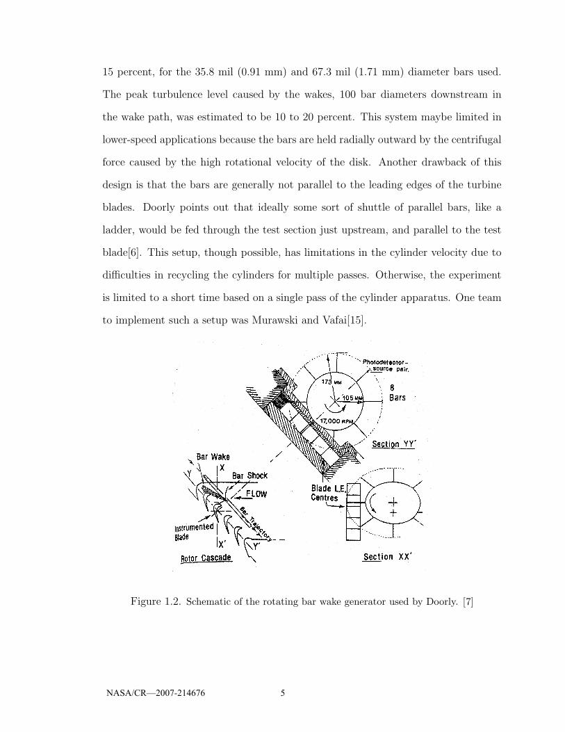
15 percent, for the 35.8 mil (0.91 mm) and 67.3 mil (1.71 mm) diameter bars used.
The peak turbulence level caused by the wakes, 100 bar diameters downstream in
the wake path, was estimated to be 10 to 20 percent. This system maybe limited in
lower-speed applications because the bars are held radially outward by the centrifugal
force caused by the high rotational velocity of the disk. Another drawback of this
design is that the bars are generally not parallel to the leading edges of the turbine
blades. Doorly points out that ideally some sort of shuttle of parallel bars, like a
ladder, would be fed through the test section just upstream, and parallel to the test
blade[6]. This setup, though possible, has limitations in the cylinder velocity due to
difficulties in recycling the cylinders for multiple passes. Otherwise, the experiment
is limited to a short time based on a single pass of the cylinder apparatus. One team
to implement such a setup was Murawski and Vafai[15].
Figure 1.2. Schematic of the rotating bar wake generator used by Doorly. [7]
NASA/CR—2007-214676 5

A 1.64 ft/s (0.5 m/s) to 16.4 ft/s (5 m/s) cylinder velocity could be achieved by
Murawski and Vafai[15] with their test setup. They used a moving shuttle positioned
in the floor and ceiling of the test section. This setup is shown in Figure 1.3 A. The
shuttles could accept 0.374 in. (9.5 mm) diameter cylinders, at a 3.61 in. (91.7 mm)
pitch and were positioned such that they located the cylinders 2.5 in. (6.35 cm) up-
stream of the test blades. Measurements at different, but constant, cylinder velocities
showed that increasing the cylinder velocity, and thus the wake velocity, decreases
the relative inlet flow angle[15]. According to there results, the inlet flow angle varied
from approximately 4o at the highest cylinder and free stream velocity to 36o at the
lowest conditions. This variation in inlet angle helps to illustrate the importance of
using moving-wake generators in turbine research. Based on results of Halstead et
al.[12], Murawski and Vafai estimated the wake width at the leading edge of the test
blade to be 0.75 in. (1.905 cm) with a total velocity deficit of 25 percent. Also they
estimated the peak turbulence intensity in the cylinder wake to be 14 percent with
a wake width of 1.22 in. (3.096 cm). Blade passing frequencies from 12 Hz to 52 Hz
could be achieved. Murawski and Vafai found that the secondary flow vortex struc-
ture is dependent on the the blade passing to axial chord flow frequency. Thus it is
important to have flexibility in the rate of the disturbance propagation(generation)
or blade passing frequency.
Some researchers have used cylinders mounted on conveyor belts. This cylin-
der/conveyor setup would then be passed through the test section, upstream of the
test cascade, to produce the unsteady disturbance and because of the conveyor sys-
tem experiments could easily be run for longer periods of time. Schobeiri and Pappu
took this type of approach for their research and could achieve cylinder velocities of
up to 20 ft/s (6 m/s)[19]. In their case, the cylinders passed close to the leading edge
of the blades on the forward pass and then were routed outside of the test section, to
NASA/CR—2007-214676 6

A: Passing shuttle of cylinders.[15] B: Cylinders mounted on belt.[19]
Figure 1.3. Additional examples of cylinder setups.
wrap around the outside of the test section. This setup is shown in Figure 1.3 B.
So far all of the apparatuses mentioned have been similar in that the plain in
which the cylinders pass are parallel to the plain of the blade cascade. Work done by
Pfeil et al.[16] on laminar to turbulent boundary layer transition caused by unsteady
wakes on a flat plate, used what is considered a squirrel cage design as the disturbance
generator. For their work, cylinders were mounted near the edge of a 23.6 in. (0.6
m) diameter rotatable disk, parallel to the axis of rotation[16]. The disk was then
positioned inside the tunnel, just upstream of the flat plate being investigated. Like
the others, this setup had the flexibility of different and controllable cylinder velocities
based on the rotational velocity of the disk. The blade passing frequency could also
be adjusted by changing the cylinder spacing. In this design, all of the cylinders are
in the wind tunnel at all times. Variations in the rotational velocity of the disk alter
both the plate Reynolds number and frequency of the velocity fluctuations. Whereas
changes in the free-stream velocity alter the magnitude of the velocity fluctuation and
the pressure gradient over the plate. There was no data given on the capabilities of
the setup in terms of velocity fluctuations at the leading edge of the plate.
NASA/CR—2007-214676 7
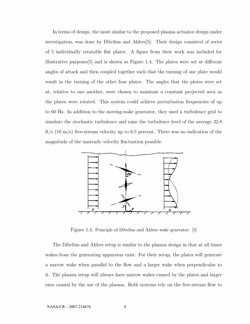
In terms of design, the most similar to the proposed plasma actuator design under
investigation, was done by Dibelius and Ahlers[5]. Their design consisted of series
of 5 individually rotatable flat plates. A figure from their work was included for
illustrative purposes[5] and is shown as Figure 1.4. The plates were set at different
angles of attack and then coupled together such that the turning of one plate would
result in the turning of the other four plates. The angles that the plates were set
at, relative to one another, were chosen to maintain a constant projected area as
the plates were rotated. This system could achieve perturbation frequencies of up
to 60 Hz. In addition to the moving-wake generator, they used a turbulence grid to
simulate the stochastic turbulence and raise the turbulence level of the average 32.8
ft/s (10 m/s) free-stream velocity up to 6.5 percent. There was no indication of the
magnitude of the unsteady velocity fluctuation possible.
Figure 1.4. Principle of Dibelius and Ahlers wake generator. [5]
The Dibelius and Ahlers setup is similar to the plasma design in that at all times
wakes from the generating apparatus exist. For their setup, the plates will generate
a narrow wake when parallel to the flow and a larger wake when perpendicular to
it. The plasma setup will always have narrow wakes caused by the plates and larger
ones caused by the use of the plasma. Both systems rely on the free-stream flow to
NASA/CR—2007-214676 8

carry the unsteady disturbances downstream. Also, both are designed to be oriented
perpendicular to the free-stream flow Dibelius and Ahlers showed the ability of their
configuration to be able to simulate the unsteady wake flow of a moving blade row
by the use of a similarity plot of wake profiles at various downstream positions, with
the theoretical Gaussian far wake profile, and a comparison of the magnitudes of the
velocity deficits to real test cases.[5]
1.3 Objectives
The main objective is a proof of concept of a simple and efficient method for
simulating a moving wake using plasma actuators. This concept could then be used
to build an apparatus that will simulate the disturbances caused by the stators or
rotors of a turbine over a more versatile and realistic range of velocities and blade
passing frequencies than current mechanical means. This moving-wake generator
could then be used for turbine research.
To achieve this objective, different types of setups, starting with airfoils will be
tested along with different types of plasma actuators. The concept has the design
constraint that the apparatus can not be placed any closer than 10 in. (25.4 cm) to
the turbine test blade. Thus, it is desired to obtain results comparable to what can
be achieved by mechanical means at this distance. The results of these tests will be
summarized and where possible, compared to the mechanical models.
Lastly, the pros and cons of the setups will be discussed to pick the most viable
direction for the practical application. Once this is done, the results can be used
as a phase two starting point to start testing a full array of actuators and actually
propagate a disturbance across a test section.
NASA/CR—2007-214676 9
CHAPTER 2
EXPERIMENTAL SETUP
The experiments and results described in this thesis were all performed in the
Plasma Flow Control Laboratory at the University of Notre Dame’s Hessert Labo-
ratory for Aerospace Research. This chapter discusses the experimental setup that
was implemented for this research. One side note, more depth of the setup is given
in this chapter than normal because the author of this thesis was responsible for and
performed most of the construction required for the facility.
2.1 Wind Tunnel
The wind tunnel used is a new facility that was designed and constructed for
the use of the research presented in this thesis. It is a general purpose wind tunnel
that will be available for future research and as a test-bed to aid in the setup of
experiments that will use other facilities in the Hessert Laboratory which have more
stringent scheduling constraints.
Work on this particular facility started the summer of 2000 in the form of draw-
ings1. Over that summer, refinements were made to the design, construction materials
were located, ordered, and purchased. Due to the construction of another wind tunnel
for the Hessert Laboratory, actual construction of this wind tunnel did not start until
the autumn of 2001, and was completed in the spring of 2002. The summer of 2002
1Original drawings were done by Catherine Corke
NASA/CR—2007-214676 10
was spent instrumenting and setting up the experimental equipment, such as, the
traversing system, hot-wire anemometer, and pressure transducer that were needed
for the experiments.
Similar to the other wind tunnels at the Hessert Laboratories, the new wind tunnel
is an open-return design. But unlike most of the other wind tunnels this tunnel is a
pusher-type as opposed to a typical draw-down type. The primary difference is that
the fan is the first stage, and thus it is located upstream of the test section. In this
configuration, the fan pushes air through the tunnel. The advantage of the pusher
design is that the tunnel operates at a pressure higher than that of the surrounding
atmosphere. This is beneficial in that if the tunnel should have or develop an air
leak, the higher pressure will force the air out of the tunnel. This is preferred because
it will tend to thin the boundary layer, reducing the possibility of causing a flow
separation. In a typical draw-down tunnel, air leaks tend to thicken the boundary
layer and cause unwanted disturbances in the test section.
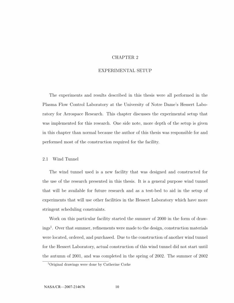
An 18.25 in. (46.355 cm) diameter Chicago Blower Design 47 adjustable-pitch
vane axial fan was chosen based on previous experience with this model and a cost
savings as it was bought in conjunction with another Chicago Blower fan. The fan is
rated for 6000 CFM (170 CMM), a total pressure of 8.681 inWG (2160 Pa), and has a
maximum rotational speed of 3500 RPM. The variable pitch airfoils can be adjusted
manually from a pitch setting of -2 to 8 degrees. The fan is driven by an electric 15
HP, 3 phase, Duty Master AC-motor made by Reliance Electric. The fan unit was
purchased through Industrial Air Solutions, Inc at a net cost of $4270. This includes
the price of the Baldor #ID15H210 − E variable frequency drive and the shipping
costs. The fan is shown in Figure 2.1.
Following the fan comes a circular-to-square transition section. This was made
by Troeger & Co. metal fabrication specialists from 16 gauge CRS(cold-rolled-steel)
NASA/CR—2007-214676 11
Figure 2.1. Wind tunnel fan before final assembly.
at a cost of $465. Due to an oversight after a design change, this transition section
went from an 18.00 in. (45.72 cm) interior dimension (ID) circle, instead of the 18.25
in. (46.36 cm) ID of the fan, to a 29.50 in. (74.93 cm) ID square. To fix this a 3/4
in. (1.90 cm) thick wood spacer ring was added in the joint between the fan and
transition section to blend the two diameters. Silicon caulk was then used to seal the
joint.
The next stage in the wind tunnel is the flow conditioning section. This condition-
ing element consists of a honeycomb section and 5 screens. The honeycomb section
was purchased from Plascore Inc. at a cost of $172 plus shipping. It is a 29.5 in.
(74.93 cm) square made up of 1/4 in. (6.35 mm) diameter straws that are 5.0 in.
(12.7 cm) long. The honeycomb section is used as a flow straightener to remove any
swirl from the flow caused by the fan. The screen material used was purchased from
Albany International at a cost of $316. The screens are made up of 7.5 mil (0.191
mm) 316 stainless steel wire with a mesh of 28 by 28 wires per 1.0 in. (2.54 cm).
This diameter wire and spacing gives a solidity of approximately 38 percent. Based
NASA/CR—2007-214676 12

on the work of Loehrke[14], it was decided that only five screens were needed. Given
the wire diameter of the screens, the optimum distance for the turbulence produced
by the screens to decay to its minimum level was 9.00 in. (22.7 cm)[14]. To maintain
this spacing, five 29.5 in. (74.93 cm) square box sections 9.00 in. (22.7 cm) deep
were built out of 3/4 in. (1.905 cm) birch veneered plywood. The box sections can
be seen in Figure 1. This figure also shows the 1.0 in. (2.54 cm) equal-leg angle iron
flanges which were drilled and bolted to the plywood to provide a means of bolting
the sections together. Strips of 1/8 in. (3.175 mm) DURO 60 black commercial neo-
prene rubber, purchased from the Royal Rubber Company, were glued to the angle
iron flanges to seal the screen box sections and to aid in maintaining the tension in
the screens.
Figure 2.2. The screen boxes before final assembly.
Prior to assembly of the flow conditioning section of the tunnel, the inside of
the screen boxes were painted and the corners were sealed with silicon caulk. For
assembly, the screens were stretched on a specially made rack and while under tension,
the screen boxes were bolted together around the screens. The screen tensioning rack
NASA/CR—2007-214676 13

was then removed and the screens were trimmed to the size of the screen box sections.
One screen was placed in between each screen box, and one between the last screen
box and the contraction. The honeycomb was placed in the first screen box and was
pushed flat up against the first screen.
The next wind tunnel element in the series is the contraction section. A 5th order
polynomial curve was chosen for the contraction shape. A very gradual length-to-
diameter ratio of 2:1 was originally chosen however, due to space limitations in the
laboratory, this number was reduced to 1:1. The contraction was fabricated in-house
and is not symmetric.
The inlet is a 29.5 in. (74.93 cm) ID square that reduces to an 18.0 in. (45.72
cm) ID wide by 12.0 in. (30.48 cm) ID tall rectangular outlet. This gives an area
reduction ratio of 4:1. Based on these boundary conditions, the equation for the 5th
order polynomial curve for the top and bottom contour can be seen as Equation 2.1
and as Equation 2.2 for the sides.
z = −2.350× 10−6x5 + 1.733× 10−4x4 − 3.408× 10−3x3 + 14.75 (2.1)
z = −1.544× 10−6x5 + 1.139× 10−4x4 − 2.240× 10−6x3 + 14.75 (2.2)
To set the contraction shape, points calculated using Equations 2.1 and 2.2 were
laid out on yellow pine 2x4’s. These were cut, sanded, and used for the ribs of the
contraction. A picture of the partially completed contraction can be seen in Figure
2.3. In order to lay out the shape of the top, bottom, and side panels, the three
dimensional intersection, of the two dimensional 5th order polynomial plains had to
be found and transformed into two dimensions. Once this was done, the coordinates
could be laid out on a piece 1/4 in. (6.35 mm) thick tempered hardboard, which
was used as the paneling. The hardboard intersections, on the outside corners of
the contraction, were first screwed together and then reinforced with fiber glass cloth
NASA/CR—2007-214676 14

and resin. As with the screen sections, the inside of the contraction was painted
and silicon caulk was used to seal the corners. Angle iron flanges were attached to
the ends of the contraction walls for joining the contraction to the neighboring wind
tunnel pieces.
Figure 2.3. The contraction during construction.
Just downstream of the contraction comes the test section. It has a rectangular
cross section of 18.0 in. (45.72 cm) ID wide by 12.0 in. (30.48 cm) ID high and
is 3.0 ft. (91.44 cm) long. It is made from 1/2 in. (12.7 mm) Plexiglas. Again,
angle iron was used for the connecting flanges. A 30 in. (76.20 cm) section of the
top panel is removable to allow access to the models. This section, along with the
following two sections, were all placed on an easily movable wheeled bench. Having
all the downstream elements of the wind tunnel mounted on the wheeled bench, and
because the test section can easily be detached from the contraction, made access
to the models quick and easy either through the front or the top of the test section.
Located in the bottom panel of the test section is a 1/2 in (12.7 mm) by 23.5 in.
(59.69 cm) slot. The slot starts 9.50 in. (24.13 cm) from the front of the test section
NASA/CR—2007-214676 15
(upstream side) and runs along the center line of the test section. The slot allows
access for the stream-wise traverse system.
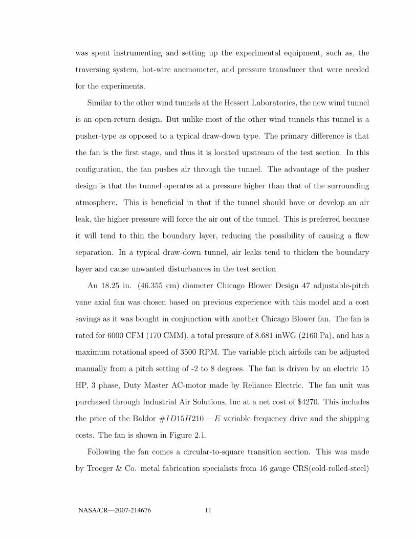
Following the test section, the flow encounters a 90o turn. The turn was designed
into the tunnel to conserve lab space and to minimize the local air disturbance in the
lab. The turn enables the air to be diffused towards the ceiling of the laboratory. The
birch veneer plywood was again used for this section along with 26 gauge, galvanized
steel, sheet metal to make the turning vanes. The vanes have a gap to cord ratio of
1:3. This was chosen to minimize the drag and thus the pressure drop through the
section[3]. A picture of this section can be seen in Figure 2.4.
Figure 2.4. Flow turning section during construction.
The final piece of the tunnel is the diffuser. This is also made from birch veneer
plywood. As mentioned earlier, this is directed towards the ceiling. It has a total
interior angle of 12 degrees to maximize the pressure recovery while trying to avoid
separation and thus a stalled diffuser. A picture of the finished tunnel is shown in
Figure 2.5.
NASA/CR—2007-214676 16
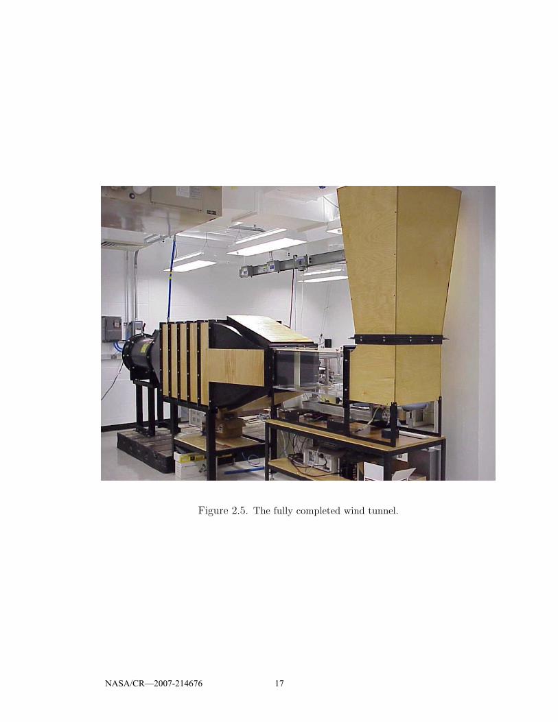
Figure 2.5. The fully completed wind tunnel.
NASA/CR—2007-214676 17

Most of the building materials, such as the plywood, hardboard, screws, bolts,
and etc. can be found at most home improvement warehouses. The steel used was
purchased in South Bend from Alro Steel and the Plexiglas was purchased from Alro
Plastics. The wood costs were approximately $140, the steel costs were approximately
$100, and the Plexiglas was also $140. Miscellaneous expenses including a special
steel cold-cutting saw blade($270 alone), screws, bolts, paint, and etc. came to about
$850 dollars. This brings the grand total for building the tunnel to roughly $6500,
excluding labor.
2.2 Traverse
After completion of the physical wind tunnel, two traversing systems were added.
These allowed motion in both the streamwise and spanwise direction of any probe(s)
added to the traversing pod. The streamwise system is a commercial aluminum
traverse whose drive screw has 20 threads per inch. This drive screw is driven by a
MO92-FD08 Superior Electric Slo-Sync stepper motor with 200 steps per revolution
and drives an aluminum slider. This gives 1000 steps per inch (2.54 cm) of linear
motion. A Velmex controller, which receives the signals sent from the computer, is
used to control the motor and perform the desired motion. The stream-wise travel
is 20 inches (50.8 cm). The Velmex controller can also be used manually to position
the aluminum slider.
Mounted to the aluminum slider of the streamwise traverse is the spanwise tra-
verse system. This traverse was designed and built by the author of this thesis. It
uses a Micro Mo Electronics, Inc AM1524-V-6-35-07 micro-motor with a 158 housing
parameter and a built-in 76:1 gear box. The stepper motor itself has 24 steps per
revolution, but with the 76:1 gearbox, this provides 1824 steps per revolution. To
change this rotary motion into a linear spanwise motion for the probe, a standard
NASA/CR—2007-214676 18
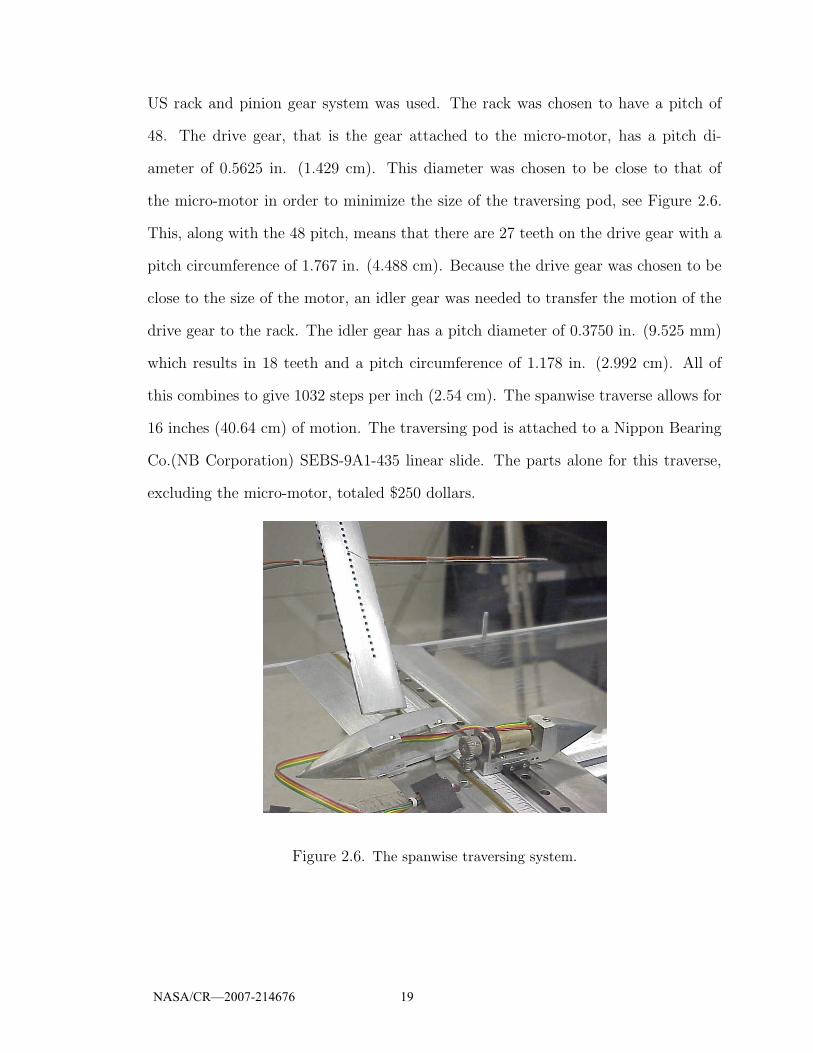
US rack and pinion gear system was used. The rack was chosen to have a pitch of
48. The drive gear, that is the gear attached to the micro-motor, has a pitch di-
ameter of 0.5625 in. (1.429 cm). This diameter was chosen to be close to that of
the micro-motor in order to minimize the size of the traversing pod, see Figure 2.6.
This, along with the 48 pitch, means that there are 27 teeth on the drive gear with a
pitch circumference of 1.767 in. (4.488 cm). Because the drive gear was chosen to be
close to the size of the motor, an idler gear was needed to transfer the motion of the
drive gear to the rack. The idler gear has a pitch diameter of 0.3750 in. (9.525 mm)
which results in 18 teeth and a pitch circumference of 1.178 in. (2.992 cm). All of
this combines to give 1032 steps per inch (2.54 cm). The spanwise traverse allows for
16 inches (40.64 cm) of motion. The traversing pod is attached to a Nippon Bearing
Co.(NB Corporation) SEBS-9A1-435 linear slide. The parts alone for this traverse,
excluding the micro-motor, totaled $250 dollars.
Figure 2.6. The spanwise traversing system.
NASA/CR—2007-214676 19
2.3 Data Acquisition
An in-house fabricated computer running Linux was used for data acquisition and
control. It utilizes an ECS L7S7A2 (sis 746 chip-set) mother board with an AMD
Athlon XP 2.8 GHz 333 processor with 512MB RAM. For the Analog-to-Digital
conversion, a PowerDAQ II PCI simultaneous-sampling multi-function PD2-MFS-4-
1M/12 board was used. This is a 12 bit board that gives a maximum resolution of
2.44 mV/bit. Three of the four available channels were used in the single ended input
configuration, and all other analog inputs on the STP-9616 connector board where
grounded.
The single-ended acquisition mode is set using the software of the data acquisition
programs. Using Linux, the programs2, written in the C programming language, were
modified to control the stepper motors for the traverses and to acquire the signals
from the hot-wire, Pitot probe, and thermocouple.
A Dantec CTA(Constant-Temperature-Anemometer) 56C17 Bridge was used with
a Dantec a CTA 56C01 Main Frame as the hot-wire anemometer. This sent the voltage
fluctuations from the bridge, caused by the heat transfer from the hot-wire, first to
a Hewlett Packard(now Agilent) 34401A multi-meter, then to a voltage-gain circuit,
and lastly to the Power-DAQ card.
Two circuits built by the author of this thesis were used in the data-acquisition
setup. The first was a gain circuit for the hot-wire to better utilize the full range of AD
board. The circuit used four LM741 operational amplifiers. One op-amp was placed
on both ends of the circuit to serve as unity-gain followers, in order to isolate the
circuit from the other electronics. The first of the remaining two op-amps, along with
resistors, were used to offset the DC signal component such that the signal from the
2The original programs were written by Junhui Huang and used the PowerDAQ libraries
NASA/CR—2007-214676 20

hot-wire, with the wind tunnel off, was close to the minimum range of the AD board,
which was -5.0 V. The last op-amp was used to gain the signal. The combination of
resistors were chosen to give a gain of 6.33, the highest possible signal gain for upper
range of the AD board, which is 5.0 V, at the maximum wind velocity used during
the calibration of the hot-wire. A schematic of the circuit can be seen in Figure 2.7.
Figure 2.7. Circuit diagram of the gain circuit used.
The second circuit used served as a simple RC low-pass filter. The cut off frequency
for the filter is controlled by the choice of resistor and capacitor. This frequency was
chosen to be 135 KHz, using an 11.75 KΩ resistor and a 0.10 µF capacitor. An
illustration of this circuit is shown in Figure 2.8.
The three signals were passed through the low-pass filter and acquired through
three single-ended channels of the AD board. The signals were all referenced to the
same instrument ground.
NASA/CR—2007-214676 21
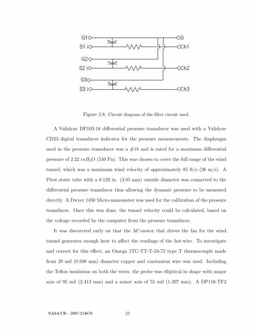
Figure 2.8. Circuit diagram of the filter circuit used.
A Validyne DP103-18 differential pressure transducer was used with a Validyne
CD23 digital transducer indicator for the pressure measurements. The diaphragm
used in the pressure transducer was a #18 and is rated for a maximum differential
pressure of 2.22 inH2O (550 Pa). This was chosen to cover the full range of the wind
tunnel, which was a maximum wind velocity of approximately 85 ft/s (26 m/s). A
Pitot static tube with a 0.120 in. (3.05 mm) outside diameter was connected to the
differential pressure transducer thus allowing the dynamic pressure to be measured
directly. A Dwyer 1430 Micro-manometer was used for the calibration of the pressure
transducer. Once this was done, the tunnel velocity could be calculated, based on
the voltage recorded by the computer from the pressure transducer.
It was discovered early on that the AC-motor that drives the fan for the wind
tunnel generates enough heat to affect the readings of the hot-wire. To investigate
and correct for this effect, an Omega 5TC-TT-T-24-72 type T thermocouple made
from 20 mil (0.508 mm) diameter copper and constantan wire was used. Including
the Teflon insulation on both the wires, the probe was elliptical in shape with major
axis of 95 mil (2.413 mm) and a minor axis of 55 mil (1.397 mm). A DP116-TF2
NASA/CR—2007-214676 22

miniature panel thermometer was used to relate the reading of the thermocouple to a
temperature. This combination had a range of±200oF . The thermocouple was placed
close to the hot-wire to record the local temperature. With the local temperature
known, the hot-wire voltages could be corrected. The equation for the temperature
correction that was used is presented as Equation 2.3.
vhwcor=
1√
1− αor−1
(Texp − Tref )vhw (2.3)
To summarize and better illustrate the complete setup, a flow chart is presented
in Figure 2.9. This shows a basic sketch of the test section with the instrumentation.
Figure 2.9. Flow chart of data acquisition setup.
During the experiments, only mean and RMS voltage data were of interest to the
investigators. It was therefore decided to take longer sampling periods at lower sam-
pling rates. A sampling rate of 2.0 KHz was chosen, and only 6 seconds of contiguous
data was taken, although longer sampling periods would have been better. However,
due to the large number spanwise locations tested, which ranged from 60 to 90 points
NASA/CR—2007-214676 23
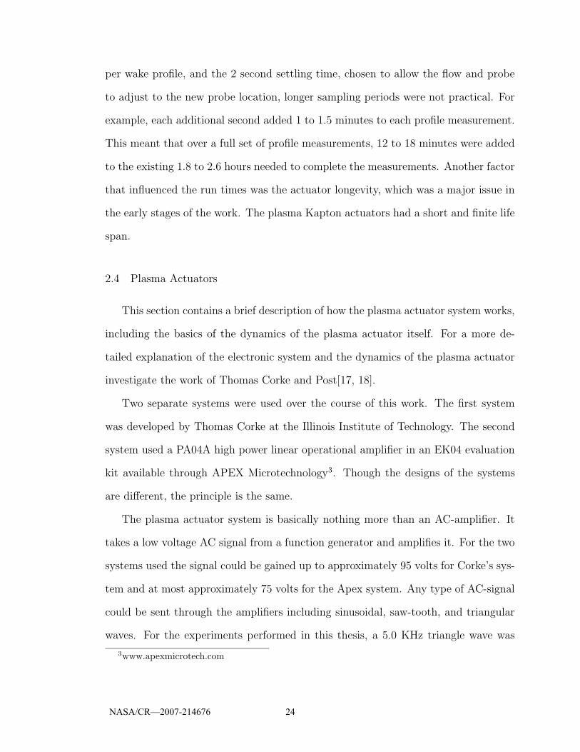
per wake profile, and the 2 second settling time, chosen to allow the flow and probe
to adjust to the new probe location, longer sampling periods were not practical. For
example, each additional second added 1 to 1.5 minutes to each profile measurement.
This meant that over a full set of profile measurements, 12 to 18 minutes were added
to the existing 1.8 to 2.6 hours needed to complete the measurements. Another factor
that influenced the run times was the actuator longevity, which was a major issue in
the early stages of the work. The plasma Kapton actuators had a short and finite life
span.
2.4 Plasma Actuators
This section contains a brief description of how the plasma actuator system works,
including the basics of the dynamics of the plasma actuator itself. For a more de-
tailed explanation of the electronic system and the dynamics of the plasma actuator
investigate the work of Thomas Corke and Post[17, 18].
Two separate systems were used over the course of this work. The first system
was developed by Thomas Corke at the Illinois Institute of Technology. The second
system used a PA04A high power linear operational amplifier in an EK04 evaluation
kit available through APEX Microtechnology3. Though the designs of the systems
are different, the principle is the same.
The plasma actuator system is basically nothing more than an AC-amplifier. It
takes a low voltage AC signal from a function generator and amplifies it. For the two
systems used the signal could be gained up to approximately 95 volts for Corke’s sys-
tem and at most approximately 75 volts for the Apex system. Any type of AC-signal
could be sent through the amplifiers including sinusoidal, saw-tooth, and triangular
waves. For the experiments performed in this thesis, a 5.0 KHz triangle wave was
3www.apexmicrotech.com
NASA/CR—2007-214676 24
used. Potentiometers controlled the amount of the gain, which was monitored with
an oscilloscope. After the signal leaves the first gain circuit, it is sent to a transformer
to be gained further. Some initial experiments used transformers with a winding ratio
of 30:1, but most of the experiments used transformers that had 140 windings. This
means a gain of 140, which for translates to an AC-signal up to 13.3 KVpp for the first
system. The plasma systems were comprised of multiple op-amps and transformers
so that the AC-signals could be supplied to multiple electrodes.
This signal was then sent to the plasma actuator. An illustration of one is shown
in Figure 2.10. Basically, it is two electrodes, that slightly overlap, separated by
a dielectric material. As with any circuit, the voltage potential at any given point
depends on where that point is referenced to. One electrode of the actuator can
either be grounded or attached to another channel of the plasma system. If one
electrode is grounded, the highest voltage potential across the actuator is half of the
voltage supplied to the opposite electrode. This is because the AC-signal has no DC
component and the furthest away from zero(ground) the signal gets is half of its peak-
to-peak amplitude. If however, the opposite electrode is attached to a second channel
from the plasma system, then the full potential, in this case up to 13.3 KV, can be
achieved. This is because the second channel can be sent the same AC-signal but 180o
out of phase. This way, the signals reference each and the difference between them is
the voltage potential across the actuator. The two channel setup was used for most
of the experiments presented. Unfortunately, the power of the plasma actuator could
not be obtained because the voltage potential across the actuator and the current
through it could not be directly measured. However, the voltage potential across the
actuator could be estimated by multiplying the voltage sent to the transformers by
the number of windings of the transformer.
NASA/CR—2007-214676 25

Figure 2.10. Illustration of a plasma actuator.
Also shown in Figure 2.10 is an indication of the direction of the body force
that the plasma actuator produces. Some additional comments and figures will be
presented during the discussion of the test setups in Section 2.5.
2.5 Test and Actuator Configurations
Due to the large number of experimental configurations tested and variations of
each, the configurations were broken down into three main areas. These areas were
designated as Airfoils, Flat Plates and Uniform Flat Plates and will be discussed in
their respective chapters. With in these three main areas, there are 6 basic config-
urations. These will be denoted by configurations 1-6 and will be discussed in this
section. The configuration designation and a short description of the respective setup
is summarized at the end of this section in Table 2.1.
Other than the flow visualization, all of the experiments that were conducted
involved wake profiles at different downstream locations of the test piece(s). Two
main experiments were performed in the wakes of the different configurations. The
first is referred to as stream profiles and the second is referred to as power profiles.
Initially there were two sets of free-stream conditions being used as a check of the
diversity of the moving-wake generator in terms of its application. Normally the wind
NASA/CR—2007-214676 26
tunnels free-stream velocity would be set based on a desired Reynolds number for the
test piece under investigation. Initially this was the case here as well but because
the idea behind the moving-wake generator is to use it as an experimental tool in
other research applications, the free-stream velocities were of more importance then
the Reynolds number of the airfoil(s) or flat plate(s) being tested. The free-stream
velocity used in the different stages of this work will be discussed in their respective
configuration setups.
The stream profiles were the first experiments conducted. These consisted of wake
profiles at the following cord lengths downstream of the trailing edge of the test piece:
0.5, 1, 2, 3, 4 and 5. They are called stream profiles because the main variable, other
than having the actuator ‘off’ or ‘on’, is the streamwise position. When the effect
of the actuator was tested, a wake profile at a particular downstream location was
first conducted with the actuator ‘off’, with the probe transversing towards one side
of the test section. Immediately following this profile, the actuator would be turned
‘on’ and another wake profile would be performed with the probe now traversing in
the opposite direction. This would return the probe to the original starting position.
Following this, the streamwise traverse would be manually adjusted to position the
probe at the next downstream location.
What is being referred to as power profiles were all conducted 5 cord lengths
downstream of the trailing edge of the test piece. These tests were an investigation
into the effects of varying the voltage potential across the actuator, which is equivalent
to varying the power of the actuator and is where the designation ‘power profile’ came
from. In these cases, the hot-wire probe would be moved in one direction for one dial
setting and then be moved in the opposite direction for the next dial setting. In all
the cases, the voltage potential always started at zero and was increased. These tests
were interchanged with the stream profiles for comparison.
NASA/CR—2007-214676 27

In addition to these, a few experiments were done to investigate the position
dependence of the flat plates. These cases were conducted in a similar manner to
the power profiles, but instead of changing the voltage potential, the relative position
of the plates was changed. The main purpose of doing this was to chose the plate
arrangement that gave the most uniform wakes in terms of width and velocity deficit.
2.5.1 Configuration 1
The first configuration to be discussed is Configuration 1. The experiments per-
formed under this configuration used one or two NACA 0018 airfoil(s) with a 3.1 in.
(7.87 cm) chord, with two mounting holes, 2 in. (5.08 cm) apart and centered along
the mean chord line in either end of the airfoil. Holding the airfoil were two, one
on each side, 95 mil. (2.41 mm) thick aluminum plates that could be attached with
screws to the test section to ensure consistent placement of the airfoil(s). One of these
plates can be seen in the top of Figure 2.114. Two series of holes, 2.0 in. (5.08 cm)
apart from one another, were made in the aluminum plates. The holes had a spacing
of 0.5 in. (1.27 cm) with the center hole on the center line of the test section when
the plates were attached to the test section. The series of holes were offset from the
front edge of the plate such that when the airfoil(s) was attached, it’s leading edge
was 0.5 in. (1.27 cm) downstream of the beginning edge of the test section. The
series of holes allowed for the space between two airfoils to varied in 0.50 in. (cm)
increments. One additional set of holes was added 0.25 in. (cm) from the center hole
to allow for 0.25 in. (cm) space increase to the 0.50 in. (cm) space increments.
In the case when only one airfoil was tested, it was oriented vertically along the
4Also shown in this figure is a clear Plexiglas replacement plate, used for the flow visualization,
and different mounting brackets, used for the flat plates, which will be discussed in later sections
concerning the flat plates.
NASA/CR—2007-214676 28
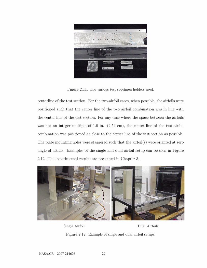
Figure 2.11. The various test specimen holders used.
centerline of the test section. For the two-airfoil cases, when possible, the airfoils were
positioned such that the center line of the two airfoil combination was in line with
the center line of the test section. For any case where the space between the airfoils
was not an integer multiple of 1.0 in. (2.54 cm), the center line of the two airfoil
combination was positioned as close to the center line of the test section as possible.
The plate mounting holes were staggered such that the airfoil(s) were oriented at zero
angle of attack. Examples of the single and dual airfoil setup can be seen in Figure
2.12. The experimental results are presented in Chapter 3.
Single Airfoil Dual Airfoils
Figure 2.12. Example of single and dual airfoil setups.
NASA/CR—2007-214676 29
As mentioned before, to investigate the utility of the moving-wake generator being
developed, two free-stream velocities were chosen for the experiments. These were
chosen to be within the range of Reynolds numbers that corresponded to the turbine
research that was being done by another experimentalist5. In that research, plasma
actuators are being used to control flow separation in a cascade of Pratt & Whitney
Pack-B low pressure turbine blades. Blades with an axial of chord 6.28 in. (15.95 cm)
are being tested. The first free-stream velocity was chosen to be 31 ft/s (9.45 m/s).
This corresponds to a Reynolds number of 100K for the turbine blade in air at typical
atmospheric conditions which were 29.5 in-Hg (749.3 mm-Hg) and 70oF (21oC). The
second velocity used was 54 ft/s (16.5 m/s) which corresponds to a Reynolds number
of 175K for the Pack-B blades.
Four cases, other than the non-actuated case, were investigated. These cases had
the same actuator design but different actuator placements. The active edge of the
actuator was placed in one of the following locations: at the leading edge, just before
the maximum thickness point, at the point of maximum thickness, and just after the
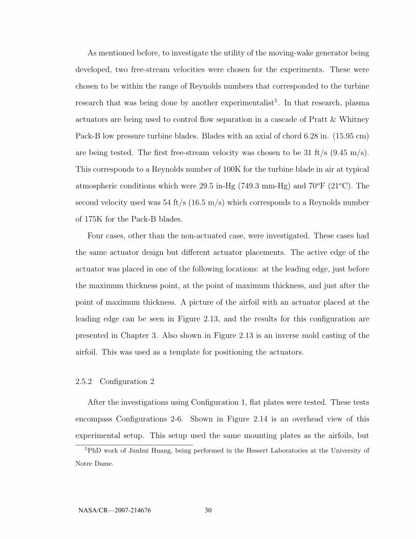
point of maximum thickness. A picture of the airfoil with an actuator placed at the
leading edge can be seen in Figure 2.13, and the results for this configuration are
presented in Chapter 3. Also shown in Figure 2.13 is an inverse mold casting of the
airfoil. This was used as a template for positioning the actuators.
2.5.2 Configuration 2
After the investigations using Configuration 1, flat plates were tested. These tests
encompass Configurations 2-6. Shown in Figure 2.14 is an overhead view of this
experimental setup. This setup used the same mounting plates as the airfoils, but
5PhD work of Junhui Huang, being performed in the Hessert Laboratories at the University of
Notre Dame.
NASA/CR—2007-214676 30
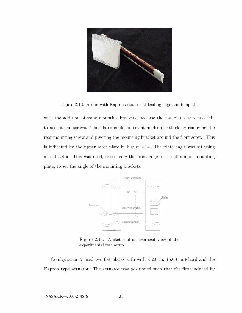
Figure 2.13. Airfoil with Kapton actuator at leading edge and template.
with the addition of some mounting brackets, because the flat plates were too thin
to accept the screws. The plates could be set at angles of attack by removing the
rear mounting screw and pivoting the mounting bracket around the front screw. This
is indicated by the upper most plate in Figure 2.14. The plate angle was set using
a protractor. This was used, referencing the front edge of the aluminum mounting
plate, to set the angle of the mounting brackets.
Figure 2.14. A sketch of an overhead view of theexperimental test setup.
Configuration 2 used two flat plates with with a 2.0 in. (5.08 cm)chord and the
Kapton type actuator. The actuator was positioned such that the flow induced by
NASA/CR—2007-214676 31
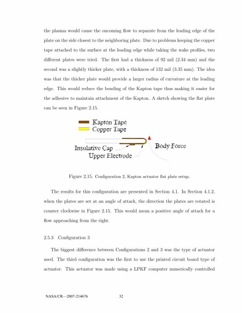
the plasma would cause the oncoming flow to separate from the leading edge of the
plate on the side closest to the neighboring plate. Due to problems keeping the copper
tape attached to the surface at the leading edge while taking the wake profiles, two
different plates were tried. The first had a thickness of 92 mil (2.34 mm) and the
second was a slightly thicker plate, with a thickness of 132 mil (3.35 mm). The idea
was that the thicker plate would provide a larger radius of curvature at the leading
edge. This would reduce the bending of the Kapton tape thus making it easier for
the adhesive to maintain attachment of the Kapton. A sketch showing the flat plate
can be seen in Figure 2.15.
Figure 2.15. Configuration 2, Kapton actuator flat plate setup.
The results for this configuration are presented in Section 4.1. In Section 4.1.2,
when the plates are set at an angle of attack, the direction the plates are rotated is
counter clockwise in Figure 2.15. This would mean a positive angle of attack for a
flow approaching from the right.
2.5.3 Configuration 3
The biggest difference between Configurations 2 and 3 was the type of actuator
used. The third configuration was the first to use the printed circuit board type of
actuator. This actuator was made using a LPKF computer numerically controlled
NASA/CR—2007-214676 32

(CNC) milling machine. The LPKF milling machine is prototyping machine designed
to manufacture prototype circuit boards. For these cases, the plate orientation was
such that the induced velocity was in the channel between the two adjacent plates
and directed upstream. The aim was to separate the flow from the plate to reduce or
block the flow between the plates, essentially creating a larger body.
During these tests, two different actuator electrode setups were investigated. The
first setup had an 8.00 in. (20.32 cm) lower electrode and the second had a 4.75 in.
(12.07 cm) lower electrode. Both of these lengths had an upper and lower electrode
width of 1.0 in. (2.54 cm) and the upper electrodes were 0.25 in. (6.35 mm) longer
than the lower electrode. This enabled both sides of the upper electrode to extend
0.125 in. (3.18 mm) past the edges of the lower electrode. Also, the upper electrode
overlapped the lower by 62 mil (1.59 mm) and the active actuator edge of the actuator
was moved 1.0 in. (2.54 cm) from the leading edge to the mid-chord of the plate.
One other difference between this configuration and Configuration 2 is the leading
edge contour. Because what is considered the lower electrode extended to the leading
edge of the plate, the leading edge was shaped to a 1/4 ellipse. The leading edge is
shown in Figure 2.16. It can be seen that the direction of the velocity component
induced by the plasma actuator is upstream on one side of the plate and downstream
on the other. In the case of the Kapton actuators, the second component of forcing is
suppressed by being pressed against the airfoil or plate and being covered by Kapton.
The results for this configuration are presented in Section 4.2. It is important to
note here that the results presented in that section refer to negative angles of attack.
As with Configuration 2, this angle is referenced to a flow approaching from the right
as shown in Figure 2.16. This is important due to the asymmetric leading edge. At
the negative angle the flow is less likely to separate than if the plates were at positive
angles relative to the flow.
NASA/CR—2007-214676 33
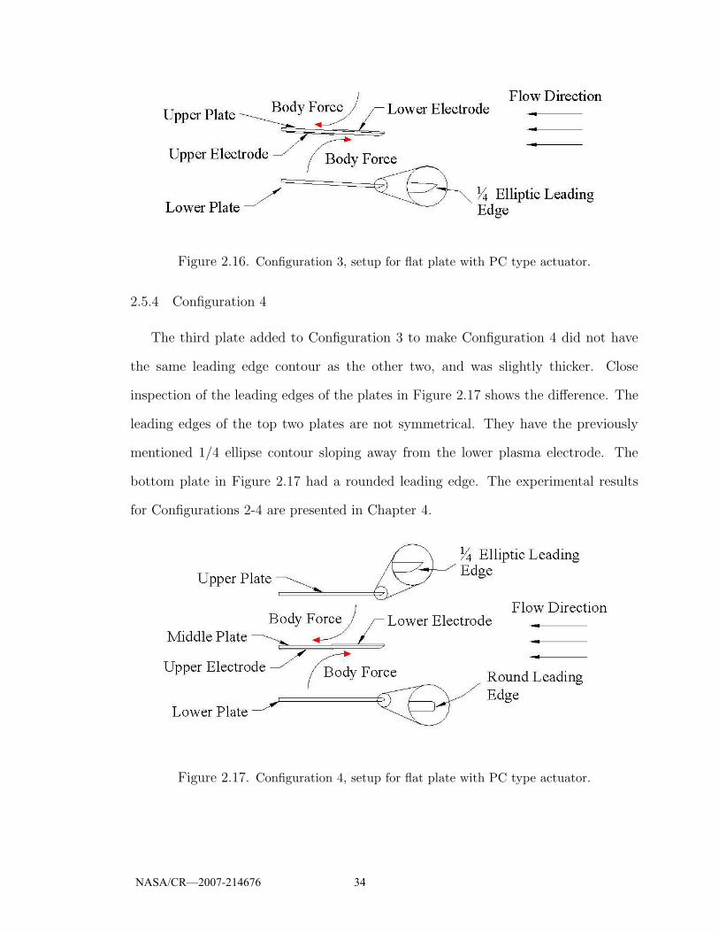
Figure 2.16. Configuration 3, setup for flat plate with PC type actuator.
2.5.4 Configuration 4
The third plate added to Configuration 3 to make Configuration 4 did not have
the same leading edge contour as the other two, and was slightly thicker. Close
inspection of the leading edges of the plates in Figure 2.17 shows the difference. The
leading edges of the top two plates are not symmetrical. They have the previously
mentioned 1/4 ellipse contour sloping away from the lower plasma electrode. The
bottom plate in Figure 2.17 had a rounded leading edge. The experimental results
for Configurations 2-4 are presented in Chapter 4.
Figure 2.17. Configuration 4, setup for flat plate with PC type actuator.
NASA/CR—2007-214676 34

2.5.5 Configuration 5
The 5th configuration was basically a repeat of Configuration 4, but with uniform
plates manufactured on the LPKF CNC milling machine. A 12 in. x 12 in. x 1/8
in. ( 30.38 cm x 30.48 cm x 3.18 mm), double sided copper-clad piece of FR-4 circuit
board material was secured to the milling bed so that the 3 plates could be machined
simultaneously. The copper was first machined off one side, leaving the electrode and
a small extension for a wire lead, and then the board was flipped. After flipping the
PC-board, the opposite electrode could be machined, and then the LPKF machine
would cut out the plates. The leading edges of the plate were then lightly hand sanded
to round the corners. This setup is shown in Figure 2.18.
Figure 2.18. Configuration 5, setup for flat plate with PC type actuator.
Also new to Configurations 5 and 6 was a set of mounting brackets for the flat
plates. These brackets, one of which is shown in the lower left of Figure 2.11, were
machined on an end mill out of a solid piece of Plexiglas. They were designed to have
the slots for the plates 3 mil (0.076 mm) larger than the thickness of the plates. This
was done to ensure consistency and straightness of the placement of the plates with
respect to each other.
NASA/CR—2007-214676 35
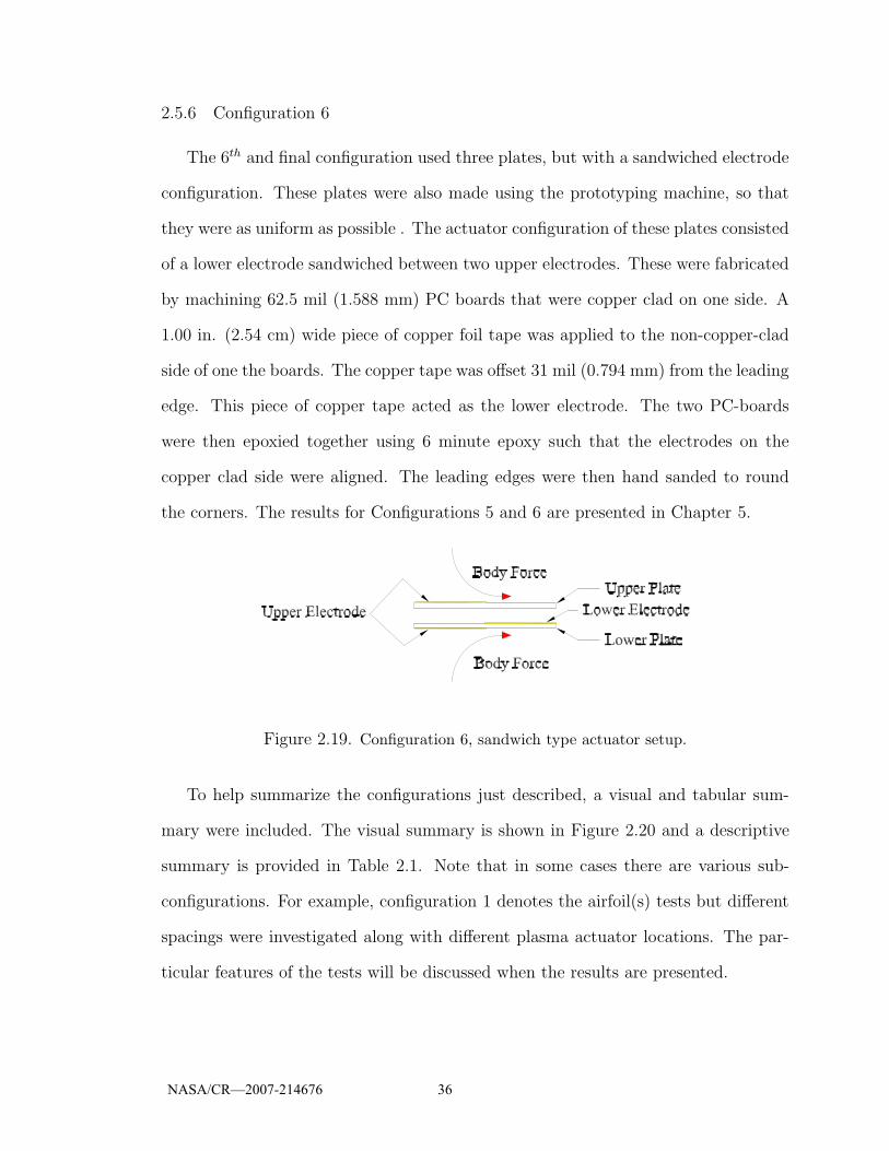
2.5.6 Configuration 6
The 6th and final configuration used three plates, but with a sandwiched electrode
configuration. These plates were also made using the prototyping machine, so that
they were as uniform as possible . The actuator configuration of these plates consisted
of a lower electrode sandwiched between two upper electrodes. These were fabricated
by machining 62.5 mil (1.588 mm) PC boards that were copper clad on one side. A
1.00 in. (2.54 cm) wide piece of copper foil tape was applied to the non-copper-clad
side of one the boards. The copper tape was offset 31 mil (0.794 mm) from the leading
edge. This piece of copper tape acted as the lower electrode. The two PC-boards
were then epoxied together using 6 minute epoxy such that the electrodes on the
copper clad side were aligned. The leading edges were then hand sanded to round
the corners. The results for Configurations 5 and 6 are presented in Chapter 5.
Figure 2.19. Configuration 6, sandwich type actuator setup.
To help summarize the configurations just described, a visual and tabular sum-
mary were included. The visual summary is shown in Figure 2.20 and a descriptive
summary is provided in Table 2.1. Note that in some cases there are various sub-
configurations. For example, configuration 1 denotes the airfoil(s) tests but different
spacings were investigated along with different plasma actuator locations. The par-
ticular features of the tests will be discussed when the results are presented.
NASA/CR—2007-214676 36

Figure 2.20. Image summary of the different configuration.
NASA/CR—2007-214676 37
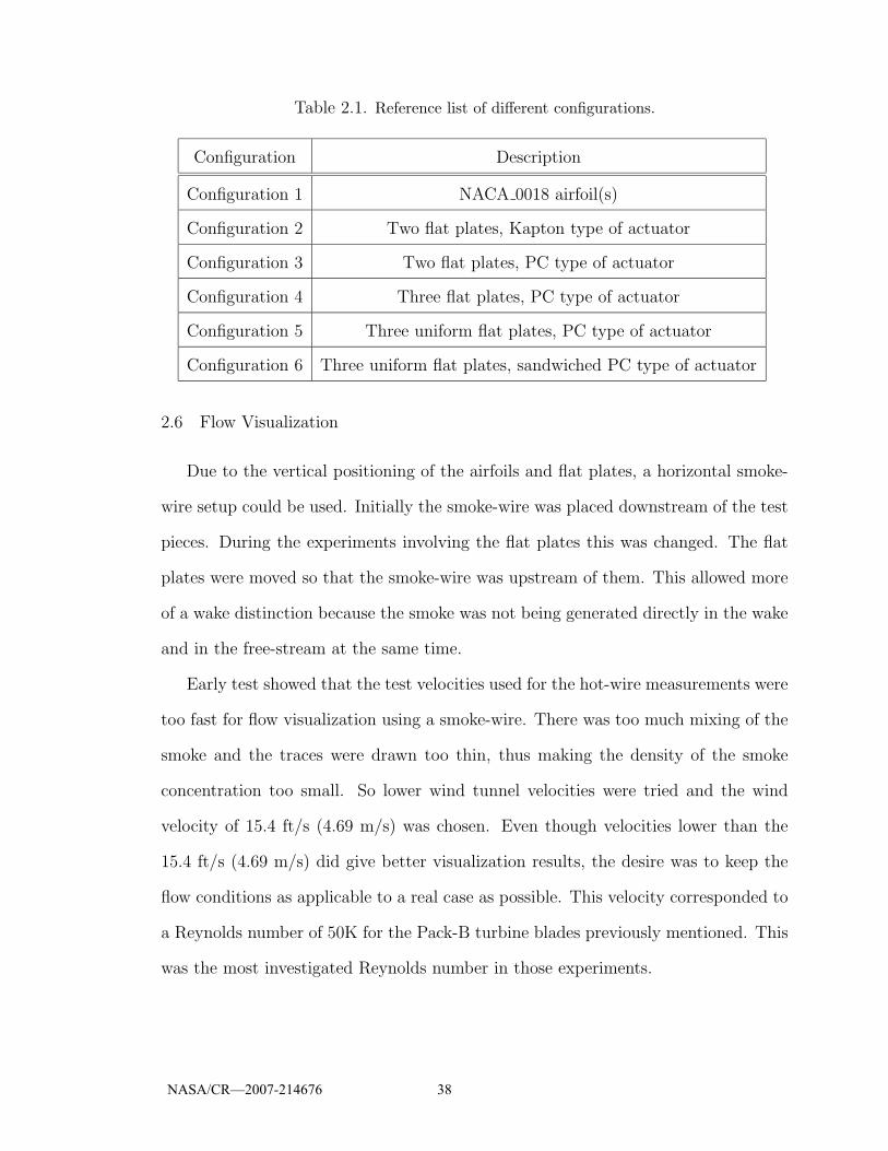
Table 2.1. Reference list of different configurations.
Configuration Description
Configuration 1 NACA 0018 airfoil(s)
Configuration 2 Two flat plates, Kapton type of actuator
Configuration 3 Two flat plates, PC type of actuator
Configuration 4 Three flat plates, PC type of actuator
Configuration 5 Three uniform flat plates, PC type of actuator
Configuration 6 Three uniform flat plates, sandwiched PC type of actuator
2.6 Flow Visualization
Due to the vertical positioning of the airfoils and flat plates, a horizontal smoke-
wire setup could be used. Initially the smoke-wire was placed downstream of the test
pieces. During the experiments involving the flat plates this was changed. The flat
plates were moved so that the smoke-wire was upstream of them. This allowed more
of a wake distinction because the smoke was not being generated directly in the wake
and in the free-stream at the same time.
Early test showed that the test velocities used for the hot-wire measurements were
too fast for flow visualization using a smoke-wire. There was too much mixing of the
smoke and the traces were drawn too thin, thus making the density of the smoke
concentration too small. So lower wind tunnel velocities were tried and the wind
velocity of 15.4 ft/s (4.69 m/s) was chosen. Even though velocities lower than the
15.4 ft/s (4.69 m/s) did give better visualization results, the desire was to keep the
flow conditions as applicable to a real case as possible. This velocity corresponded to
a Reynolds number of 50K for the Pack-B turbine blades previously mentioned. This
was the most investigated Reynolds number in those experiments.
NASA/CR—2007-214676 38
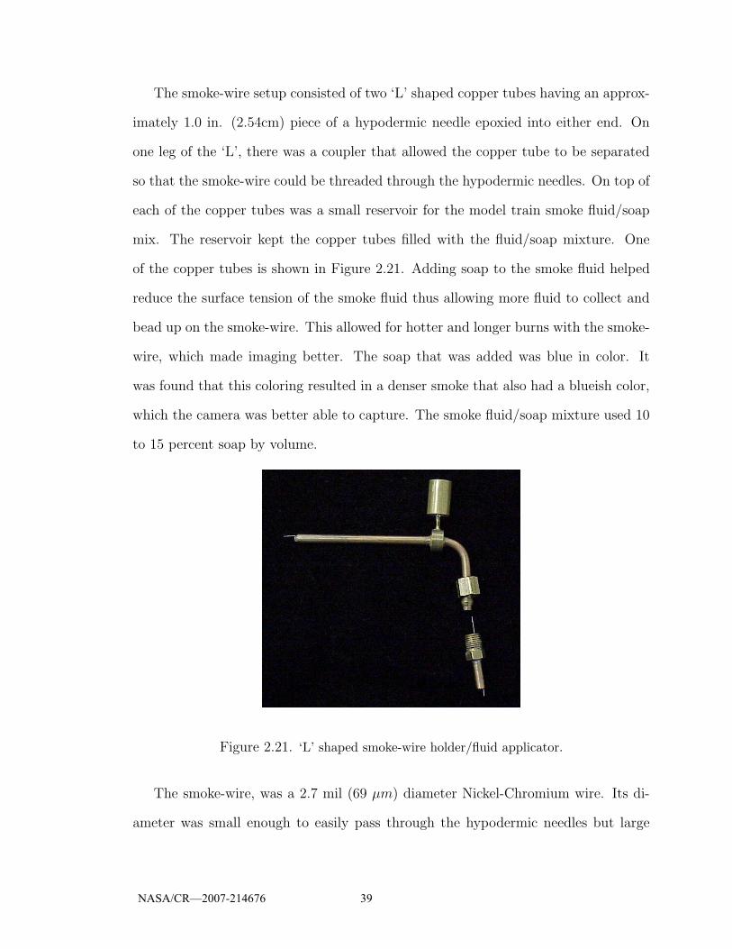
The smoke-wire setup consisted of two ‘L’ shaped copper tubes having an approx-
imately 1.0 in. (2.54cm) piece of a hypodermic needle epoxied into either end. On
one leg of the ‘L’, there was a coupler that allowed the copper tube to be separated
so that the smoke-wire could be threaded through the hypodermic needles. On top of
each of the copper tubes was a small reservoir for the model train smoke fluid/soap
mix. The reservoir kept the copper tubes filled with the fluid/soap mixture. One
of the copper tubes is shown in Figure 2.21. Adding soap to the smoke fluid helped
reduce the surface tension of the smoke fluid thus allowing more fluid to collect and
bead up on the smoke-wire. This allowed for hotter and longer burns with the smoke-
wire, which made imaging better. The soap that was added was blue in color. It
was found that this coloring resulted in a denser smoke that also had a blueish color,
which the camera was better able to capture. The smoke fluid/soap mixture used 10
to 15 percent soap by volume.
Figure 2.21. ‘L’ shaped smoke-wire holder/fluid applicator.
The smoke-wire, was a 2.7 mil (69 µm) diameter Nickel-Chromium wire. Its di-
ameter was small enough to easily pass through the hypodermic needles but large
NASA/CR—2007-214676 39
enough so that the surface tension of the smoke fluid prevented the fluid from signifi-
cantly leaking. When the wire was slid through the hypodermic tubes, it was coated
with a thin layer of fluid. The smoke fluid then formed into droplets due to a surface
tension instability. The tension of the smoke-wire itself was maintained by the weight
of two large nuts, attached to either end of the smoke-wire. Another advantage of
the use of the copper tubes is that the electrodes, that provide the current though
the smoke-wire, could be attached to the copper tubes. This prevents the tangling of
wires while the smoke-wire is used and prevents having to pass current through the
entire length of the smoke-wire.
Many different lighting setups with different backgrounds were employed in order
to obtain reasonable images. These setups ranged from using a constant light source
to using two high-powered strobe lights. It was found that the dual strode light
configuration produced the best results. It consisted of two 1540-P2 Strobolume
lamps powered by two 1540 Strobolume power supplies and controlled by two 1540-
P1 Strobolume oscillators. The controllers had the ability to send and receive a
trigger pulse. This feature was used to synchronize the two strobe lamps by having
one controller send a pulse to the adjacent controller. The two strobe lamps were
mounted side-by-side, positioned 0.50 in. (1.27 cm) apart, on a 2.50 in. (6.35) cm
by 20.0 in. (50.8 cm) and 0.25 in. (0.635 cm) thick steel plate. The steel mounting
plate was then attached to a tripod which was positioned next to the test section such
that the strobe lamps pointed at the side of the test section, which was completely
covered with cardboard except for a 1.0 in. (2.54 cm) slit centered on the smoke-wire
and running the length of the test section. This was done to reduce the addition
of light that would be reflected inside of the test section, which would intern reduce
the contrast of the illuminated smoke. The two strobes allowed for a very wide and
bright illumination of the smoke generated by the smoke-wire. An illustration of the
NASA/CR—2007-214676 40
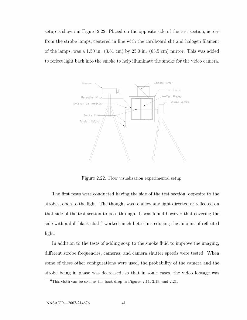
setup is shown in Figure 2.22. Placed on the opposite side of the test section, across
from the strobe lamps, centered in line with the cardboard slit and halogen filament
of the lamps, was a 1.50 in. (3.81 cm) by 25.0 in. (63.5 cm) mirror. This was added
to reflect light back into the smoke to help illuminate the smoke for the video camera.
Figure 2.22. Flow visualization experimental setup.
The first tests were conducted having the side of the test section, opposite to the
strobes, open to the light. The thought was to allow any light directed or reflected on
that side of the test section to pass through. It was found however that covering the
side with a dull black cloth6 worked much better in reducing the amount of reflected
light.
In addition to the tests of adding soap to the smoke fluid to improve the imaging,
different strobe frequencies, cameras, and camera shutter speeds were tested. When
some of these other configurations were used, the probability of the camera and the
strobe being in phase was decreased, so that in some cases, the video footage was
6This cloth can be seen as the back drop in Figures 2.11, 2.13, and 2.21.
NASA/CR—2007-214676 41

almost completely blank. The solution to this was to use a strobe frequency of 30
Hz, which was close to the frequency of the VHS video camera shutter.
A Panasonic AG-188 VHS camera was chosen over a Sony digital camera to record
the images due to the superior imaging results. The orientation of the camera to the
test section can be seen in Figure 2.22. Notice that the camera is recording the
images from a mirror that was placed on top of the test section at a 45 degree angle.
The bottom of the test section was also covered with the aforementioned black cloth
to provide greater contrast and a uniform background. It is important to point out
that because the camera was recording the images from the mirror, what the camera
recored, was an inverted image of what is actually seen when looking down into the
test section. After the video was acquired with the VHS camera, a software package
called Main Actor was used on the Linux platform to capture and digitize the images
in an uncompressed bit-map(*.bmp) format. This allowed for editing without the loss
of quality that results from editing compressed formats such as jpeg’s. To correct for
some of the effects of the mirror, as a final step, the captured images were inverted
using a program called Gimp. This was done so that the flow visualization images
and the hot-wire data could be discussed with less confusion. Some of the imaging
effects could not be corrected. For example, in some of the images presented for the
flat plates, the plates appear as though they are set at opposite angles of attack. An
example of this is shown in Figure 2.23. Note that the plates are in fact at the same
angle of attack.
2.7 Data Reduction
This section is used to present a couple miscellaneous points about the data re-
duction.
A program called MATLAB c©, developed by MathWorks, was used to fit the
NASA/CR—2007-214676 42

Zero angle of attack. 10 degree angle of attack.
Figure 2.23. Examples of imaging effects from flow visualization setup.
calibration data with a 5th order polynomial, taking in to account the temperature
correction. A FORTRAN program was used to then read in the constants and convert
the raw data, using the temperature correction, to velocities. This program also
calculated the mean and standard deviation, referred to as the RMS, of the converted
data.
To illustrate the temperature dependence, Figure 2.24 was included. This figure
shows the temperature variation during the pressure transducer calibration, along
with an extended temperature investigation. The pressure transducer calibration
comprises the first third of the time, i.e. the first 60 minutes. This large amount of
time is due to the fact that a manual micrometer was used for the calibration and at
each point, 3 readings were taken from it. After the calibration, the tunnel speed was
reduced to approximately 29 ft/s (8.84 m/s) and held for 30 min. Then the speed was
increased to approximately 43 ft/s (13.1 m/s) and held for 30 minutes, after which
the tunnel was turned off. This test was done to check if the air temperature could
be stabilized, which would mean that a temperature correction would not have to
be made. From Figure 2.24 it is obvious that the air temperature is very dependent
on the flow velocity. These temperature variations workout give velocity over esti-
mates on the order of 5 percent at 30 ft/s (9.1 m/s) and 3.5 percent at 80 ft/s (24
m/s). As mentioned earlier, the thermocouple was added to be able to correct for the
NASA/CR—2007-214676 43
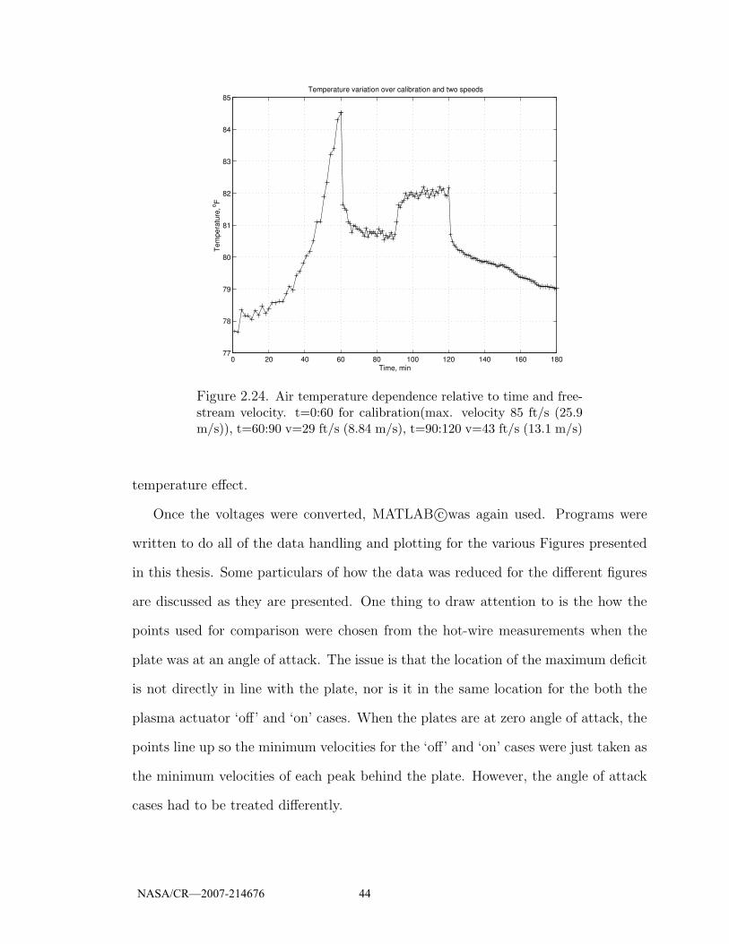
0 20 40 60 80 100 120 140 160 18077
78
79
80
81
82
83
84
85
Time, min
Tem
pera
ture
, o F
Temperature variation over calibration and two speeds
Figure 2.24. Air temperature dependence relative to time and free-stream velocity. t=0:60 for calibration(max. velocity 85 ft/s (25.9m/s)), t=60:90 v=29 ft/s (8.84 m/s), t=90:120 v=43 ft/s (13.1 m/s)
temperature effect.
Once the voltages were converted, MATLAB c©was again used. Programs were
written to do all of the data handling and plotting for the various Figures presented
in this thesis. Some particulars of how the data was reduced for the different figures
are discussed as they are presented. One thing to draw attention to is the how the
points used for comparison were chosen from the hot-wire measurements when the
plate was at an angle of attack. The issue is that the location of the maximum deficit
is not directly in line with the plate, nor is it in the same location for the both the
plasma actuator ‘off’ and ‘on’ cases. When the plates are at zero angle of attack, the
points line up so the minimum velocities for the ‘off’ and ‘on’ cases were just taken as
the minimum velocities of each peak behind the plate. However, the angle of attack
cases had to be treated differently.
NASA/CR—2007-214676 44

To help illustrate this problem, Figure 2.25 from Chapter 6 is presented. This
shows three select stream profiles with actuator ‘off’, ‘on’, and the difference between
them, shifted by 1. Because the moving-wake generator is going to be placed in a
fixed location, it is important to know exactly what the variation in the free-stream
is going to be relative to a fixed spanwise location. The way that this was handled
was to find the minimum velocity value for the plasma ‘off’ case behind the plate
with the plasma actuator. This then fixed the spanwise location. The value used
for comparison was taken from the actuator ‘on’ case at the same spanwise location.
This is justified because upon setup, the moving-wake generator could be shifted to
have the spanwise location, where the velocity fluctuation of interest is occurring,
coincide with the desired downstream spanwise location, maybe the stagnation point
on the test blade. In the first subplot is a sketch reflecting the plate orientation and
location that the data was taken. The horizontal line indicated by the letter ‘A’ is the
location of minimum velocity of the actuator ‘off’ case, and thus the y-location where
the data was taken for comparison. The horizontal line indicated by the letter ‘B’ is
in line with the center of the plate. The line indicated by the letter ‘C’ represents the
angle of attack of the plate and the projected area. The vertical distance between
the ends of this line are drawn to scale with the actual width of the projected area
of the plate. The length, angle, or the location of the line in no other way represent
the actual location of the plate.
NASA/CR—2007-214676 45

0.7 0.8 0.9 1 1.1
−1
−0.5
0
0.5
1
u/uinf
0.5c
0.7 0.8 0.9 1 1.1
−1
−0.5
0
0.5
1
u/uinf
1c
0.7 0.8 0.9 1 1.1
−1
−0.5
0
0.5
1
u/uinf
y/c
5c
Diff.OffOn
A B
C
Figure 2.25. Select stream profiles of an actuator ‘off’ and ‘on’case plotted with difference between them. A-Location minimumvelocity of the actuator ‘off’ case. B-Indication of center of the platearea blockage. C-Represents the angle of attack of the plate andprojected area.
NASA/CR—2007-214676 46
CHAPTER 3
RESULTS: AIRFOIL
This chapter presents all off the results from the airfoil testing for Configuration
1. This includes hot-wire measurements and flow visualization. The hot-wire mea-
surements for the single airfoil are presented first, followed the twin airfoils, and lastly
the flow visualization results are presented. This follows the test order in which the
results were obtained.
3.1 Single Airfoil
The initial design idea for the moving-wake generator was to use symmetric airfoils
set at zero angle of attack. For this a NACA 0018 airfoil with a 3.1 in. (7.87 cm)
chord was chosen as the first test specimen. Ideally, a NACA 0009 or NACA 0012
of similar chord length would have been chosen but molds for these airfoils were not
available at the start of the testing. However, the mold for the NACA 0018 was
available from previous research and was deemed a reasonable starting point for the
tests. The reason for choosing an airfoil was that of practicality. A thin symmetric
airfoil at zero angle of attack will produce a small wake relative to its maximum
thickness. The thickness of the airfoil would add strength to the blade and make it
easier to mount. This would be beneficial to larger test sections in that the larger
spans could be easily bridged. Under the aerodynamic loads, the added thickness, in
contrast to simply using a flat plate, would add strength making the airfoil less likely
NASA/CR—2007-214676 47

to deflect, vibrate, or twist. Another advantage of the airfoil is the round leading
edge. A sharp leading edge or flat plate is very sensitive to positioning relative to
the flow. The slightest angle can cause flow separation to occur, where as a round
leading edge reduces this sensitivity.
3.1.1 Wake Profiles
The first experiments conducted on the airfoil were hot-wire measurements. The
type of measurements performed were streamwise velocity profiles behind the unac-
tuated, single airfoil. A detailed explanation of the test setup can be seen in Section
2.5.1 of this thesis. The stream profiles were performed to establish the basic charac-
teristics and downstream structure of the airfoils’ wake. The intent was to obtain a
base or control case to have as a datum. This case could then be used for comparison
when the actuator(s) were attached to the airfoil, and when an additional airfoil was
added to the test section. This was intended to make any effects produced by adding
an actuator(s) or airfoil more apparent. Recall from Section 2.5.1 that two different
free-stream velocities were used, namely 31 ft/s (9.45 m/s), which corresponds to a
Reynolds number of 100K and is referred to as the low Reynolds number case, and
54 ft/s (16.5 m/s), which corresponds to a Reynolds number of 175K and is referred
to as the high Reynolds number case. Recall that these Reynolds numbers are based
on the setup for the Pack-B turbine blades.
The first figure presented, Figure 3.1, shows the mean velocity profiles for the
low Reynolds number velocity case. The corresponding RMS profile is presented in
Figure 3.2. Other than at the 1/2 chord downstream location, the profiles appear as
expected. The 1/2 chord location shows some velocity variations close to the airfoil
and some instrumentation drift, reflected in the variation of the free-stream velocity
at either end of the profile. In these figures, and all of the profiles to be presented, the
NASA/CR—2007-214676 48
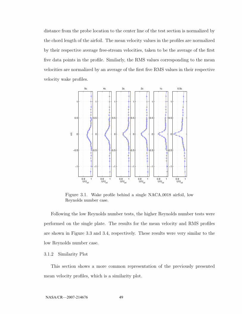
distance from the probe location to the center line of the test section is normalized by
the chord length of the airfoil. The mean velocity values in the profiles are normalized
by their respective average free-stream velocities, taken to be the average of the first
five data points in the profile. Similarly, the RMS values corresponding to the mean
velocities are normalized by an average of the first five RMS values in their respective
velocity wake profiles.
0.9 1
−1
−0.5
0
0.5
1
U/Uinf
0.5c
0.9 1
−1
−0.5
0
0.5
1
U/Uinf
1c
0.9 1
−1
−0.5
0
0.5
1
U/Uinf
2c
0.9 1
−1
−0.5
0
0.5
1
U/Uinf
3c
0.9 1
−1
−0.5
0
0.5
1
U/Uinf
4c
0.9 1
−1
−0.5
0
0.5
1
U/Uinf
x/c
5c
Figure 3.1. Wake profile behind a single NACA 0018 airfoil, lowReynolds number case.
Following the low Reynolds number tests, the higher Reynolds number tests were
performed on the single plate. The results for the mean velocity and RMS profiles
are shown in Figure 3.3 and 3.4, respectively. These results were very similar to the
low Reynolds number case.
3.1.2 Similarity Plot
This section shows a more common representation of the previously presented
mean velocity profiles, which is a similarity plot.
NASA/CR—2007-214676 49

0 50
−1
−0.5
0
0.5
1
Urms
/Uinf, rms
0.5c
0 50
−1
−0.5
0
0.5
1
Urms
/Uinf, rms
1c
0 50
−1
−0.5
0
0.5
1
Urms
/Uinf, rms
2c
0 50
−1
−0.5
0
0.5
1
Urms
/Uinf, rms
3c
0 50
−1
−0.5
0
0.5
1
Urms
/Uinf, rms
4c
0 50
−1
−0.5
0
0.5
1
Urms
/Uinf, rms
x/c
5c
Figure 3.2. Corresponding RMS profile behind a single NACA 0018airfoil, low Reynolds number case.
0.9 1
−1
−0.5
0
0.5
1
U/Uinf
0.5c
0.9 1
−1
−0.5
0
0.5
1
U/Uinf
1c
0.9 1
−1
−0.5
0
0.5
1
U/Uinf
2c
0.9 1
−1
−0.5
0
0.5
1
U/Uinf
3c
0.9 1
−1
−0.5
0
0.5
1
U/Uinf
4c
0.9 1
−1
−0.5
0
0.5
1
U/Uinf
x/c
5c
Figure 3.3. Wake profile behind a single NACA 0018 airfoil, highReynolds number case.
NASA/CR—2007-214676 50
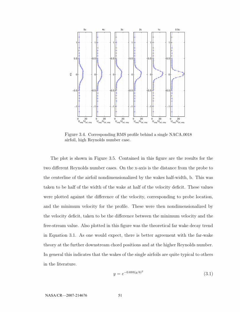
0 20
−1
−0.5
0
0.5
1
Urms
/Uinf, rms
0.5c
0 20
−1
−0.5
0
0.5
1
Urms
/Uinf, rms
1c
0 20
−1
−0.5
0
0.5
1
Urms
/Uinf, rms
2c
0 20
−1
−0.5
0
0.5
1
Urms
/Uinf, rms
3c
0 20
−1
−0.5
0
0.5
1
Urms
/Uinf, rms
4c
0 20
−1
−0.5
0
0.5
1
Urms
/Uinf, rms
x/c
5c
Figure 3.4. Corresponding RMS profile behind a single NACA 0018airfoil, high Reynolds number case.
The plot is shown in Figure 3.5. Contained in this figure are the results for the
two different Reynolds number cases. On the x-axis is the distance from the probe to
the centerline of the airfoil nondimensionalized by the wakes half-width, b. This was
taken to be half of the width of the wake at half of the velocity deficit. These values
were plotted against the difference of the velocity, corresponding to probe location,
and the minimum velocity for the profile. These were then nondimensionalized by
the velocity deficit, taken to be the difference between the minimum velocity and the
free-stream value. Also plotted in this figure was the theoretical far wake decay trend
in Equation 3.1. As one would expect, there is better agreement with the far-wake
theory at the further downstream chord positions and at the higher Reynolds number.
In general this indicates that the wakes of the single airfoils are quite typical to others
in the literature.
y = e−0.693(y/b)2 (3.1)
NASA/CR—2007-214676 51

−6 −4 −2 0 2 4 6
0
0.2
0.4
0.6
0.8
1
y/b
High Reynolds Number Case
0.5 c1.0 c2.0 c3.0 c4.0 c5.0 cTheo.
−6 −4 −2 0 2 4 6
0
0.2
0.4
0.6
0.8
1
y/b
(u−u
min
)/(u in
f−um
in)
Low Reynolds Number Case
0.5 c1.0 c2.0 c3.0 c4.0 c5.0 cTheo.
Figure 3.5. Similarity plots for single airfoil.
3.2 Twin Airfoils
After completion of the single airfoil testing, two NACA 0018 airfoils, mounted
side-by-side, were tested. As with the single airfoil, the first tests performed were
hot-wire measurements behind the two unactuated airfoils, to again define baseline
cases. These experiments were performed for the same two free-stream velocities
as the single airfoil case. The second set of investigations used flow visualization
techniques and are presented in Section 3.4.
3.2.1 Wake Profiles
Initially there was no knowledge of how close the two airfoils could be positioned
before their two wakes would start to interact with one another. To investigate this
NASA/CR—2007-214676 52
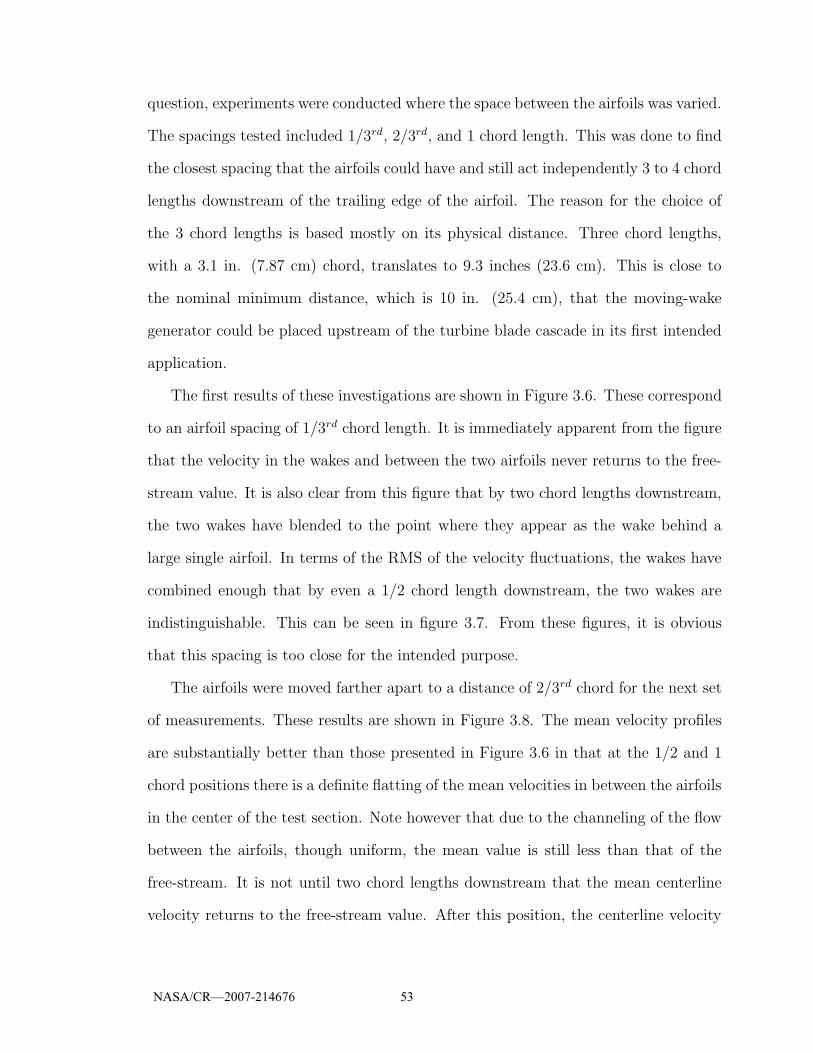
question, experiments were conducted where the space between the airfoils was varied.
The spacings tested included 1/3rd, 2/3rd, and 1 chord length. This was done to find
the closest spacing that the airfoils could have and still act independently 3 to 4 chord
lengths downstream of the trailing edge of the airfoil. The reason for the choice of
the 3 chord lengths is based mostly on its physical distance. Three chord lengths,
with a 3.1 in. (7.87 cm) chord, translates to 9.3 inches (23.6 cm). This is close to
the nominal minimum distance, which is 10 in. (25.4 cm), that the moving-wake
generator could be placed upstream of the turbine blade cascade in its first intended
application.
The first results of these investigations are shown in Figure 3.6. These correspond
to an airfoil spacing of 1/3rd chord length. It is immediately apparent from the figure
that the velocity in the wakes and between the two airfoils never returns to the free-
stream value. It is also clear from this figure that by two chord lengths downstream,
the two wakes have blended to the point where they appear as the wake behind a
large single airfoil. In terms of the RMS of the velocity fluctuations, the wakes have
combined enough that by even a 1/2 chord length downstream, the two wakes are
indistinguishable. This can be seen in figure 3.7. From these figures, it is obvious
that this spacing is too close for the intended purpose.
The airfoils were moved farther apart to a distance of 2/3rd chord for the next set
of measurements. These results are shown in Figure 3.8. The mean velocity profiles
are substantially better than those presented in Figure 3.6 in that at the 1/2 and 1
chord positions there is a definite flatting of the mean velocities in between the airfoils
in the center of the test section. Note however that due to the channeling of the flow
between the airfoils, though uniform, the mean value is still less than that of the
free-stream. It is not until two chord lengths downstream that the mean centerline
velocity returns to the free-stream value. After this position, the centerline velocity
NASA/CR—2007-214676 53

0.8 1
−1
−0.5
0
0.5
1
U/Uinf
0.5c
0.8 1
−1
−0.5
0
0.5
1
U/Uinf
1c
0.8 1
−1
−0.5
0
0.5
1
U/Uinf
2c
0.8 1
−1
−0.5
0
0.5
1
U/Uinf
3c
0.8 1
−1
−0.5
0
0.5
1
U/Uinf
4c
0.8 1
−1
−0.5
0
0.5
1
U/Uinf
x/c
5c
Figure 3.6. Wake profiles behind two NACA 0018 airfoils at 1/3rd
chord spacing, low Reynolds number case.
0 50
−1
−0.5
0
0.5
1
Urms
/Uinf, rms
0.5c
0 50
−1
−0.5
0
0.5
1
Urms
/Uinf, rms
1c
0 50
−1
−0.5
0
0.5
1
Urms
/Uinf, rms
2c
0 50
−1
−0.5
0
0.5
1
Urms
/Uinf, rms
3c
0 50
−1
−0.5
0
0.5
1
Urms
/Uinf, rms
4c
0 50
−1
−0.5
0
0.5
1
Urms
/Uinf, rms
x/c
5c
Figure 3.7. Corresponding RMS profiles behind two NACA 0018airfoils at 1/3rd chord spacing, low Reynolds number case.
NASA/CR—2007-214676 54

value slowly starts to diverge from that of the free-stream velocity value due to the
wakes mixing. This outcome is similarly shown in Figure 3.9, but the trend starts to
appear farther upstream at the 1 chord length downstream position. These results
show that although the mean velocity results are very close to the desired outcome,
the RMS results indicate that there is still some interaction between the wakes and
that the airfoils needed to be spaced further apart to obtain the desired effect.
0.8 0.9 1
−1
−0.5
0
0.5
1
U/Uinf
0.5c
0.8 0.9 1
−1
−0.5
0
0.5
1
U/Uinf
1c
0.8 0.9 1
−1
−0.5
0
0.5
1
U/Uinf
2c
0.8 0.9 1
−1
−0.5
0
0.5
1
U/Uinf
3c
0.8 0.9 1
−1
−0.5
0
0.5
1
U/Uinf
4c
0.8 0.9 1
−1
−0.5
0
0.5
1
U/Uinf
x/c
5c
Figure 3.8. Wake profiles behind two NACA 0018 airfoils at 2/3rd
chord spacing, low Reynolds number case.
The next wider spacing that still kept the airfoils symmetrically placed in the test
section was 1 chord length. The mean velocity profiles of this case are shown in Figure
3.10 and the corresponding RMS velocities profiles can be seen in Figure 3.11. As
expected by the improvement seen in the 2/3rd chord case, there was an improvement
with this larger spacing, but possibly more than what was necessary. It is clear from
Figure 3.10 that there is no significant influence of the airfoils on each other down to a
streamwise distance of 5 chord lengths. The RMS velocity profiles seen in Figure 3.11
NASA/CR—2007-214676 55
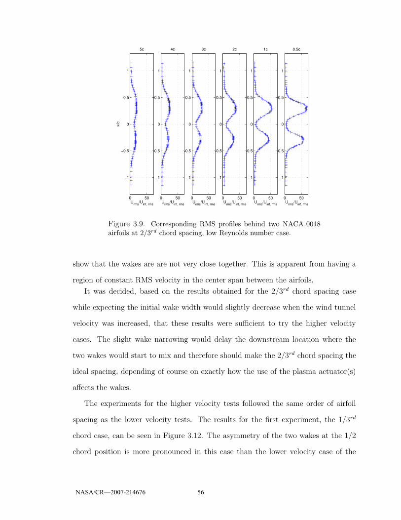
0 50
−1
−0.5
0
0.5
1
Urms
/Uinf, rms
0.5c
0 50
−1
−0.5
0
0.5
1
Urms
/Uinf, rms
1c
0 50
−1
−0.5
0
0.5
1
Urms
/Uinf, rms
2c
0 50
−1
−0.5
0
0.5
1
Urms
/Uinf, rms
3c
0 50
−1
−0.5
0
0.5
1
Urms
/Uinf, rms
4c
0 50
−1
−0.5
0
0.5
1
Urms
/Uinf, rms
x/c
5c
Figure 3.9. Corresponding RMS profiles behind two NACA 0018airfoils at 2/3rd chord spacing, low Reynolds number case.
show that the wakes are are not very close together. This is apparent from having a
region of constant RMS velocity in the center span between the airfoils.
It was decided, based on the results obtained for the 2/3rd chord spacing case
while expecting the initial wake width would slightly decrease when the wind tunnel
velocity was increased, that these results were sufficient to try the higher velocity
cases. The slight wake narrowing would delay the downstream location where the
two wakes would start to mix and therefore should make the 2/3rd chord spacing the
ideal spacing, depending of course on exactly how the use of the plasma actuator(s)
affects the wakes.
The experiments for the higher velocity tests followed the same order of airfoil
spacing as the lower velocity tests. The results for the first experiment, the 1/3rd
chord case, can be seen in Figure 3.12. The asymmetry of the two wakes at the 1/2
chord position is more pronounced in this case than the lower velocity case of the
NASA/CR—2007-214676 56
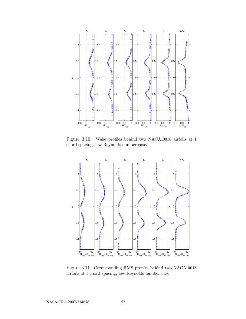
0.8 0.9 1
−1
−0.5
0
0.5
1
U/Uinf
0.5c
0.8 0.9 1
−1
−0.5
0
0.5
1
U/Uinf
1c
0.8 0.9 1
−1
−0.5
0
0.5
1
U/Uinf
2c
0.8 0.9 1
−1
−0.5
0
0.5
1
U/Uinf
3c
0.8 0.9 1
−1
−0.5
0
0.5
1
U/Uinf
4c
0.8 0.9 1
−1
−0.5
0
0.5
1
U/Uinf
x/c
5c
Figure 3.10. Wake profiles behind two NACA 0018 airfoils at 1chord spacing, low Reynolds number case.
0 50
−1
−0.5
0
0.5
1
Urms
/Uinf, rms
0.5c
0 50
−1
−0.5
0
0.5
1
Urms
/Uinf, rms
1c
0 50
−1
−0.5
0
0.5
1
Urms
/Uinf, rms
2c
0 50
−1
−0.5
0
0.5
1
Urms
/Uinf, rms
3c
0 50
−1
−0.5
0
0.5
1
Urms
/Uinf, rms
4c
0 50
−1
−0.5
0
0.5
1
Urms
/Uinf, rms
x/c
5c
Figure 3.11. Corresponding RMS profiles behind two NACA 0018airfoils at 1 chord spacing, low Reynolds number case.
NASA/CR—2007-214676 57

same spacing and the airfoil has a larger wake deficit. This asymmetry is thought to
be caused by the wakes interacting with each other. In general though, this result is
similar to the low velocity case of the same spacing in that at all of the chord positions
shown, the wakes are interacting with each other. The RMS velocity profiles show
the same trend as the lower velocity case and can be seen in Figure 3.13
0.8 1
−1
−0.5
0
0.5
1
U/Uinf
0.5c
0.8 1
−1
−0.5
0
0.5
1
U/Uinf
1c
0.8 1
−1
−0.5
0
0.5
1
U/Uinf
2c
0.8 1
−1
−0.5
0
0.5
1
U/Uinf
3c
0.8 1
−1
−0.5
0
0.5
1
U/Uinf
4c
0.8 1
−1
−0.5
0
0.5
1
U/Uinf
x/c
5c
Figure 3.12. Wake profiles behind two NACA 0018 airfoils at 1/3rd
chord spacing, high Reynolds number case.
With the airfoil spacing set at 2/3rd chord, the results again resembled those at
the same spacing that were obtained at the lower velocity. As expected, the wake
interactions were delayed slightly downstream. This can be seen in Figure 3.14. This
figure shows no significant wake interaction until 4 chord lengths downstream. This
improvement is also reflected in the corresponding RMS velocity profiles seen in Figure
3.15. They show the wakes interacting closer to the 2nd chord location, as opposed
to the 1st chord location shown in Figure 3.9 for the lower velocity case. From these
results it is clear that, at least for the two velocities tested, the 2/3rd chord spacing
NASA/CR—2007-214676 58
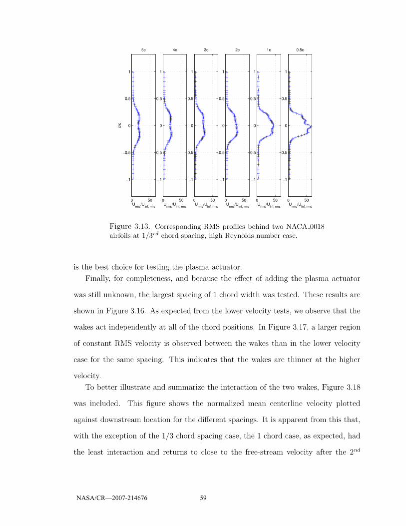
0 50
−1
−0.5
0
0.5
1
Urms
/Uinf, rms
0.5c
0 50
−1
−0.5
0
0.5
1
Urms
/Uinf, rms
1c
0 50
−1
−0.5
0
0.5
1
Urms
/Uinf, rms
2c
0 50
−1
−0.5
0
0.5
1
Urms
/Uinf, rms
3c
0 50
−1
−0.5
0
0.5
1
Urms
/Uinf, rms
4c
0 50
−1
−0.5
0
0.5
1
Urms
/Uinf, rms
x/c
5c
Figure 3.13. Corresponding RMS profiles behind two NACA 0018airfoils at 1/3rd chord spacing, high Reynolds number case.
is the best choice for testing the plasma actuator.
Finally, for completeness, and because the effect of adding the plasma actuator
was still unknown, the largest spacing of 1 chord width was tested. These results are
shown in Figure 3.16. As expected from the lower velocity tests, we observe that the
wakes act independently at all of the chord positions. In Figure 3.17, a larger region
of constant RMS velocity is observed between the wakes than in the lower velocity
case for the same spacing. This indicates that the wakes are thinner at the higher
velocity.
To better illustrate and summarize the interaction of the two wakes, Figure 3.18
was included. This figure shows the normalized mean centerline velocity plotted
against downstream location for the different spacings. It is apparent from this that,
with the exception of the 1/3 chord spacing case, the 1 chord case, as expected, had
the least interaction and returns to close to the free-stream velocity after the 2nd
NASA/CR—2007-214676 59
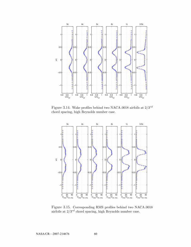
0.8 0.9 1
−1
−0.5
0
0.5
1
U/Uinf
0.5c
0.8 0.9 1
−1
−0.5
0
0.5
1
U/Uinf
1c
0.8 0.9 1
−1
−0.5
0
0.5
1
U/Uinf
2c
0.8 0.9 1
−1
−0.5
0
0.5
1
U/Uinf
3c
0.8 0.9 1
−1
−0.5
0
0.5
1
U/Uinf
4c
0.8 0.9 1
−1
−0.5
0
0.5
1
U/Uinf
x/c
5c
Figure 3.14. Wake profiles behind two NACA 0018 airfoils at 2/3rd
chord spacing, high Reynolds number case.
0 20 40
−1
−0.5
0
0.5
1
Urms
/Uinf, rms
0.5c
0 20 40
−1
−0.5
0
0.5
1
Urms
/Uinf, rms
1c
0 20 40
−1
−0.5
0
0.5
1
Urms
/Uinf, rms
2c
0 20 40
−1
−0.5
0
0.5
1
Urms
/Uinf, rms
3c
0 20 40
−1
−0.5
0
0.5
1
Urms
/Uinf, rms
4c
0 20 40
−1
−0.5
0
0.5
1
Urms
/Uinf, rms
x/c
5c
Figure 3.15. Corresponding RMS profiles behind two NACA 0018airfoils at 2/3rd chord spacing, high Reynolds number case.
NASA/CR—2007-214676 60
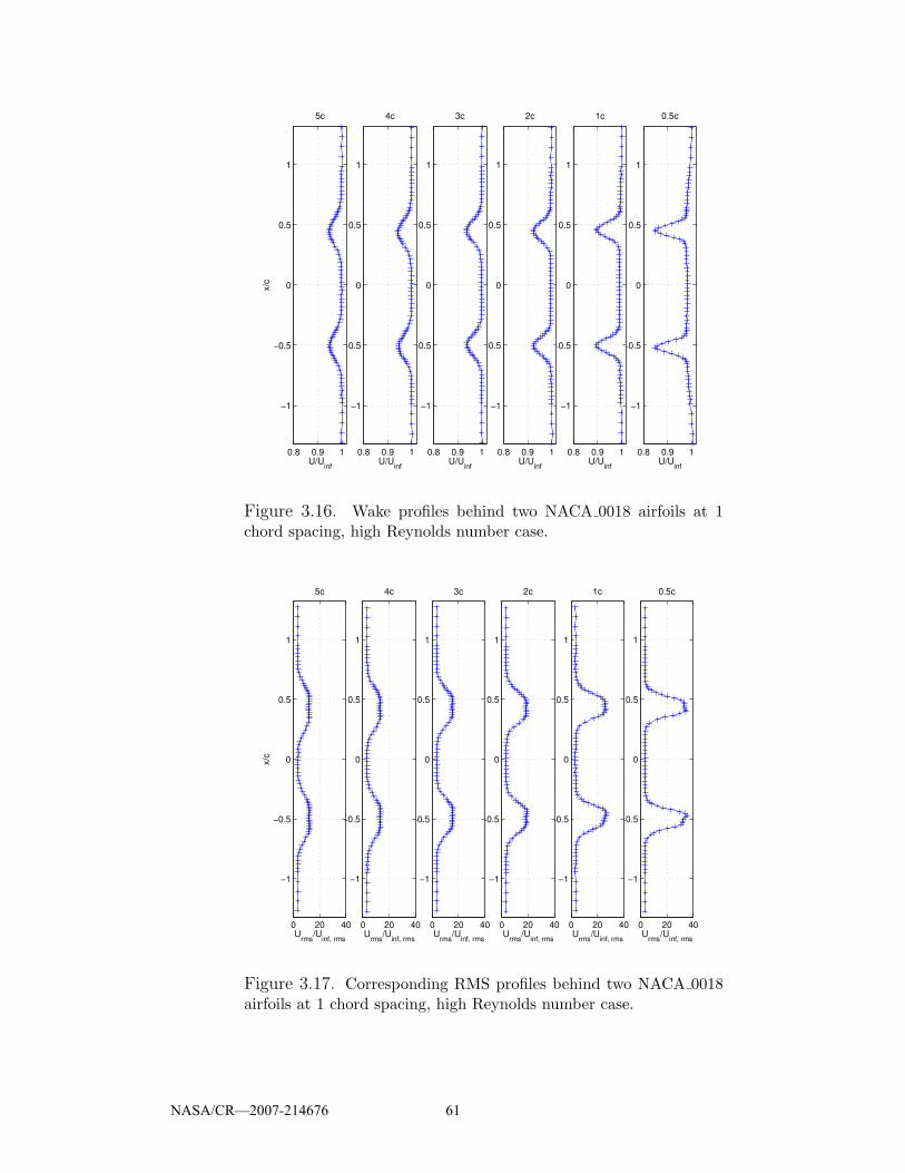
0.8 0.9 1
−1
−0.5
0
0.5
1
U/Uinf
0.5c
0.8 0.9 1
−1
−0.5
0
0.5
1
U/Uinf
1c
0.8 0.9 1
−1
−0.5
0
0.5
1
U/Uinf
2c
0.8 0.9 1
−1
−0.5
0
0.5
1
U/Uinf
3c
0.8 0.9 1
−1
−0.5
0
0.5
1
U/Uinf
4c
0.8 0.9 1
−1
−0.5
0
0.5
1
U/Uinf
x/c
5c
Figure 3.16. Wake profiles behind two NACA 0018 airfoils at 1chord spacing, high Reynolds number case.
0 20 40
−1
−0.5
0
0.5
1
Urms
/Uinf, rms
0.5c
0 20 40
−1
−0.5
0
0.5
1
Urms
/Uinf, rms
1c
0 20 40
−1
−0.5
0
0.5
1
Urms
/Uinf, rms
2c
0 20 40
−1
−0.5
0
0.5
1
Urms
/Uinf, rms
3c
0 20 40
−1
−0.5
0
0.5
1
Urms
/Uinf, rms
4c
0 20 40
−1
−0.5
0
0.5
1
Urms
/Uinf, rms
x/c
5c
Figure 3.17. Corresponding RMS profiles behind two NACA 0018airfoils at 1 chord spacing, high Reynolds number case.
NASA/CR—2007-214676 61
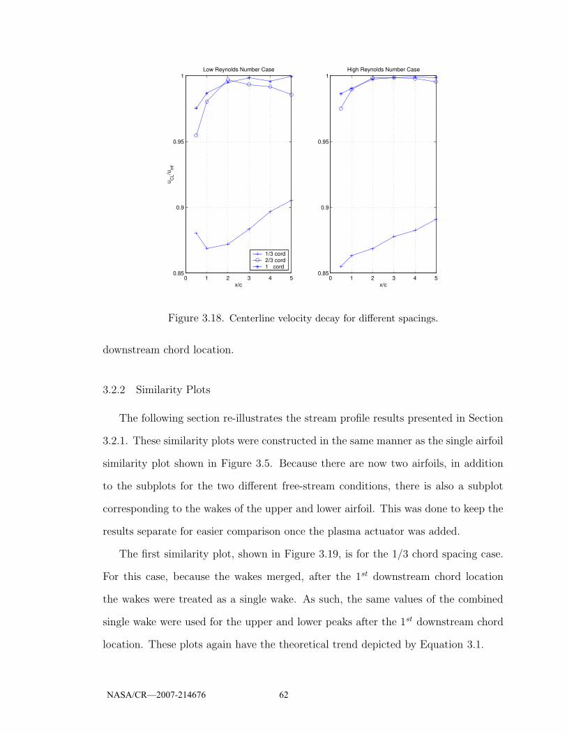
0 1 2 3 4 50.85
0.9
0.95
1
x/c
High Reynolds Number Case
0 1 2 3 4 50.85
0.9
0.95
1
x/c
u CL/u
inf
Low Reynolds Number Case
1/3 cord2/3 cord1 cord
Figure 3.18. Centerline velocity decay for different spacings.
downstream chord location.
3.2.2 Similarity Plots
The following section re-illustrates the stream profile results presented in Section
3.2.1. These similarity plots were constructed in the same manner as the single airfoil
similarity plot shown in Figure 3.5. Because there are now two airfoils, in addition
to the subplots for the two different free-stream conditions, there is also a subplot
corresponding to the wakes of the upper and lower airfoil. This was done to keep the
results separate for easier comparison once the plasma actuator was added.
The first similarity plot, shown in Figure 3.19, is for the 1/3 chord spacing case.
For this case, because the wakes merged, after the 1st downstream chord location
the wakes were treated as a single wake. As such, the same values of the combined
single wake were used for the upper and lower peaks after the 1st downstream chord
location. These plots again have the theoretical trend depicted by Equation 3.1.
NASA/CR—2007-214676 62

−6 −4 −2 0 2 4 6
0
0.2
0.4
0.6
0.8
1
(u−u
min
)/(u in
f−um
in)
Simliarity plot for Low Re. upper peaks
−6 −4 −2 0 2 4 6
0
0.2
0.4
0.6
0.8
1
y/b
(u−u
min
)/(u in
f−um
in)
Simliarity plot for Low Re. lower peaks
0.5 c1.0 c2.0 c3.0 c4.0 c5.0 cTheo.
−6 −4 −2 0 2 4 6
0
0.2
0.4
0.6
0.8
1
Simliarity plot for High Re. upper peaks
−6 −4 −2 0 2 4 6
0
0.2
0.4
0.6
0.8
1
y/b
Simliarity plot for High Re. lower peaks
Figure 3.19. Similarity Plots at 1/3 chord Spacing.
This next similarity plot is for the 2/3 chord spacing case. As seen with previous
cases, the results plotted in Figure 3.20 show better agreement with theory at the
further downstream chord locations. Overall, the plot shows good agreement with
theory.
The last spacing case is shown in Figure 3.21. This again shows good agreement
with theory.
3.3 Comparison: Single Airfoil to Twin Airfoils
The following section presents some comparisons of the hot-wire data of the single
airfoil case to the twin airfoil cases. This was done to better illustrate the effects of
the wake interactions.
NASA/CR—2007-214676 63

−6 −4 −2 0 2 4 6
0
0.2
0.4
0.6
0.8
1
(u−u
min
)/(u in
f−um
in)
Simliarity plot for Low Re. upper peaks
−6 −4 −2 0 2 4 6
0
0.2
0.4
0.6
0.8
1
y/b
(u−u
min
)/(u in
f−um
in)
Simliarity plot for Low Re. lower peaks
0.5 c1.0 c2.0 c3.0 c4.0 c5.0 cTheo.
−6 −4 −2 0 2 4 6
0
0.2
0.4
0.6
0.8
1
Simliarity plot for High Re. upper peaks
−6 −4 −2 0 2 4 6
0
0.2
0.4
0.6
0.8
1
y/b
Simliarity plot for High Re. lower peaks
Figure 3.20. Similarity Plots at 2/3 chord Spacing.
−6 −4 −2 0 2 4 6
0
0.2
0.4
0.6
0.8
1
Simliarity plot for High Re. upper peaks
−6 −4 −2 0 2 4 6
0
0.2
0.4
0.6
0.8
1
y/b
Simliarity plot for High Re. lower peaks
−6 −4 −2 0 2 4 6
0
0.2
0.4
0.6
0.8
1
(u−u
min
)/(u in
f−um
in)
Simliarity plot for Low Re. upper peaks
−6 −4 −2 0 2 4 6
0
0.2
0.4
0.6
0.8
1
y/b
(u−u
min
)/(u in
f−um
in)
Simliarity plot for Low Re. lower peaks
0.5 c1.0 c2.0 c3.0 c4.0 c5.0 cTheo.
Figure 3.21. Similarity Plots at 1 chord Spacing.
NASA/CR—2007-214676 64
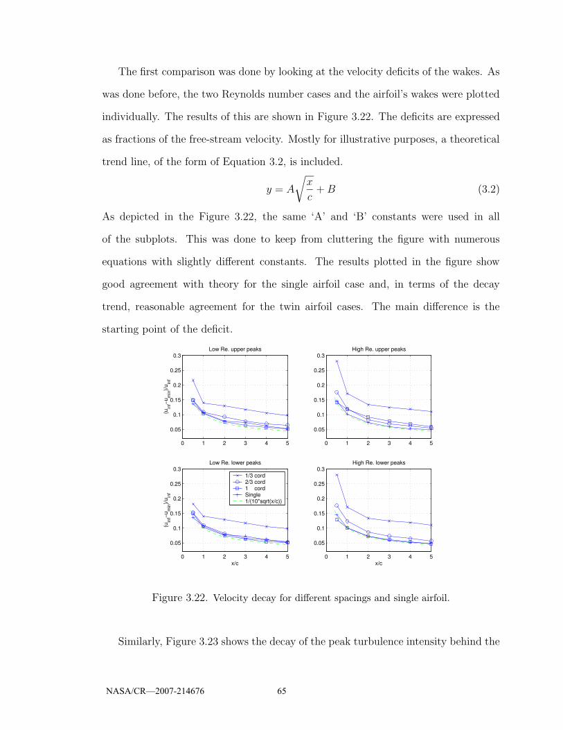
The first comparison was done by looking at the velocity deficits of the wakes. As
was done before, the two Reynolds number cases and the airfoil’s wakes were plotted
individually. The results of this are shown in Figure 3.22. The deficits are expressed
as fractions of the free-stream velocity. Mostly for illustrative purposes, a theoretical
trend line, of the form of Equation 3.2, is included.
y = A
√
x
c+B (3.2)
As depicted in the Figure 3.22, the same ‘A’ and ‘B’ constants were used in all
of the subplots. This was done to keep from cluttering the figure with numerous
equations with slightly different constants. The results plotted in the figure show
good agreement with theory for the single airfoil case and, in terms of the decay
trend, reasonable agreement for the twin airfoil cases. The main difference is the
starting point of the deficit.
0 1 2 3 4 5
0.05
0.1
0.15
0.2
0.25
0.3High Re. upper peaks
0 1 2 3 4 5
0.05
0.1
0.15
0.2
0.25
0.3
(uin
f−um
in)/u
inf
Low Re. upper peaks
0 1 2 3 4 5
0.05
0.1
0.15
0.2
0.25
0.3
x/c
High Re. lower peaks
0 1 2 3 4 5
0.05
0.1
0.15
0.2
0.25
0.3
x/c
(uin
f−um
in)/u
inf
Low Re. lower peaks
1/3 cord2/3 cord1 cordSingle1/(10*sqrt(x/c))
Figure 3.22. Velocity decay for different spacings and single airfoil.
Similarly, Figure 3.23 shows the decay of the peak turbulence intensity behind the
NASA/CR—2007-214676 65

airfoil(s). For this plot two different theoretical trends were included, one for each the
low and high Reynolds number cases. The theoretical trends of the form of Equation
3.2 were not matched perfectly or to the same cases. However, the results do show
basic agreement of the decay trends with the theory. Again, the main difference
between the cases is the initial starting point or magnitude of the turbulence at the
1/2 chord location.
0 1 2 3 4 50.02
0.04
0.06
0.08
0.1
0.12
0.14High Re. upper peaks
0 1 2 3 4 50.02
0.04
0.06
0.08
0.1
0.12
0.14
u rms/u
inf
Low Re. upper peaks
0 1 2 3 4 50.02
0.04
0.06
0.08
0.1
0.12
0.14
x/c
High Re. lower peaks
1/3 cord2/3 cord1 cordSingle1/(10*sqrt(x/c))−.01
0 1 2 3 4 50.02
0.04
0.06
0.08
0.1
0.12
0.14
x/c
u rms/u
inf
Low Re. lower peaks
1/3 cord2/3 cord1 cordSingle1/(8*sqrt(x/c))−.02
Figure 3.23. RMS decay for different spacings and single airfoil.
This last figure, Figure 3.24, shows the decay of the half width with the distance
downstream. For these cases, the theoretical form of the decay trend follows Equation
3.3.
y = A√x+B (3.3)
Again, only one representative trend was used for illustrative purposes to keep from
cluttering the figure. From this figure, it is apparent that 1/3 chord spacing, low
Reynolds number case, does not follow the theoretical trend. For the two low Reynolds
NASA/CR—2007-214676 66

number subplots, the two wakes were considered merged for all of the chord locations.
The 1/3 chord spacing, high Reynolds number, case however does seem to follow the
trend, after the 1/2 chord location where the wakes had merged and the half-width
was treated as a single wake. Inspection of the figure shows that the single airfoil
and wider twin airfoil spacings follow the same basic theoretical trend, although
the constants will be slightly different for each case. The different constants reflect
the differences in the locations where the wakes merged. The reason for different
choice of where the wakes were considered merged was based on the ability to extract
information. The wakes were considered separate for long as possible for each case.
However, some cases simply would be separate longer than others, as was the case
for the high Reynolds number case.
0 5 10 150
0.1
0.2
0.3
0.4
0.5
0.6
High Re. upper peaks
0 5 10 150
0.1
0.2
0.3
0.4
0.5
0.6
b (in
)
Low Re. upper peaks
0 5 10 150
0.1
0.2
0.3
0.4
0.5
0.6
x (in)
High Re. lower peaks
1/3 cord2/3 cord1 cordSingle1/5*sqrt(x)
0 5 10 150
0.1
0.2
0.3
0.4
0.5
0.6
x (in)
b (in
)
Low Re. lower peaks
1/3 cord2/3 cord1 cordSingle1/10*sqrt(x)+.1
Figure 3.24. Wake half-width decay for different spacings and singleairfoil.
At this point, it was decided that the results seen thus far were sufficient to proceed
with the investigations using the plasma actuator. In order to obtain a global view of
NASA/CR—2007-214676 67
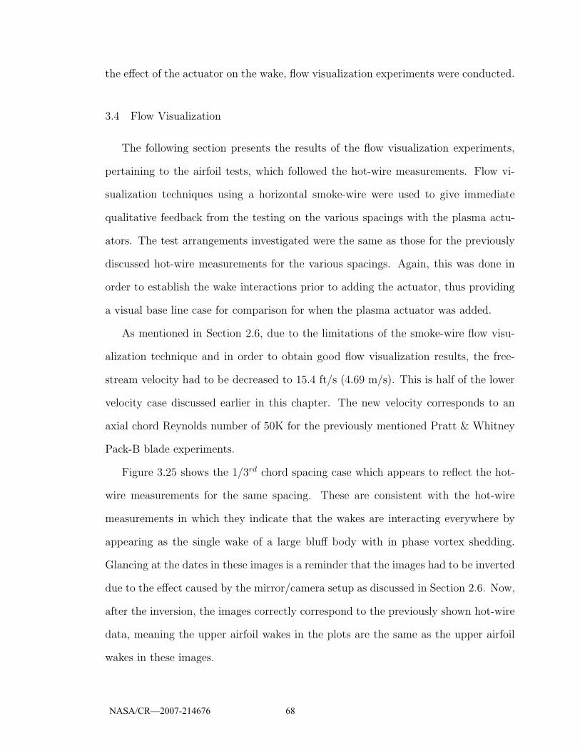
the effect of the actuator on the wake, flow visualization experiments were conducted.
3.4 Flow Visualization
The following section presents the results of the flow visualization experiments,
pertaining to the airfoil tests, which followed the hot-wire measurements. Flow vi-
sualization techniques using a horizontal smoke-wire were used to give immediate
qualitative feedback from the testing on the various spacings with the plasma actu-
ators. The test arrangements investigated were the same as those for the previously
discussed hot-wire measurements for the various spacings. Again, this was done in
order to establish the wake interactions prior to adding the actuator, thus providing
a visual base line case for comparison for when the plasma actuator was added.
As mentioned in Section 2.6, due to the limitations of the smoke-wire flow visu-
alization technique and in order to obtain good flow visualization results, the free-
stream velocity had to be decreased to 15.4 ft/s (4.69 m/s). This is half of the lower
velocity case discussed earlier in this chapter. The new velocity corresponds to an
axial chord Reynolds number of 50K for the previously mentioned Pratt & Whitney
Pack-B blade experiments.
Figure 3.25 shows the 1/3rd chord spacing case which appears to reflect the hot-
wire measurements for the same spacing. These are consistent with the hot-wire
measurements in which they indicate that the wakes are interacting everywhere by
appearing as the single wake of a large bluff body with in phase vortex shedding.
Glancing at the dates in these images is a reminder that the images had to be inverted
due to the effect caused by the mirror/camera setup as discussed in Section 2.6. Now,
after the inversion, the images correctly correspond to the previously shown hot-wire
data, meaning the upper airfoil wakes in the plots are the same as the upper airfoil
wakes in these images.
NASA/CR—2007-214676 68
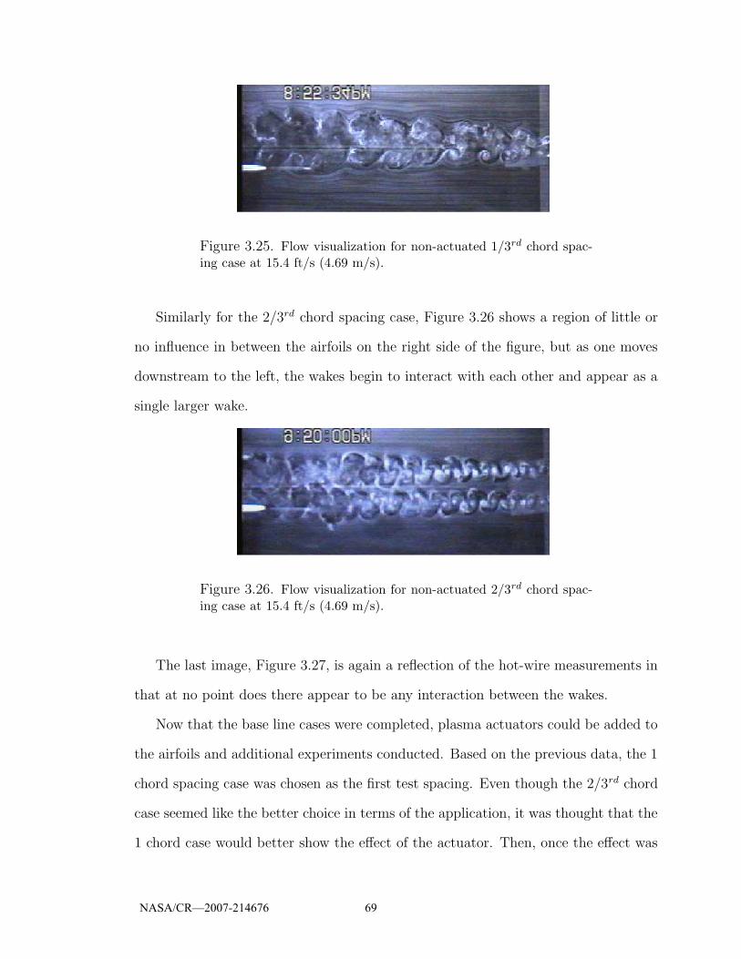
Figure 3.25. Flow visualization for non-actuated 1/3rd chord spac-ing case at 15.4 ft/s (4.69 m/s).
Similarly for the 2/3rd chord spacing case, Figure 3.26 shows a region of little or
no influence in between the airfoils on the right side of the figure, but as one moves
downstream to the left, the wakes begin to interact with each other and appear as a
single larger wake.
Figure 3.26. Flow visualization for non-actuated 2/3rd chord spac-ing case at 15.4 ft/s (4.69 m/s).
The last image, Figure 3.27, is again a reflection of the hot-wire measurements in
that at no point does there appear to be any interaction between the wakes.
Now that the base line cases were completed, plasma actuators could be added to
the airfoils and additional experiments conducted. Based on the previous data, the 1
chord spacing case was chosen as the first test spacing. Even though the 2/3rd chord
case seemed like the better choice in terms of the application, it was thought that the
1 chord case would better show the effect of the actuator. Then, once the effect was
NASA/CR—2007-214676 69
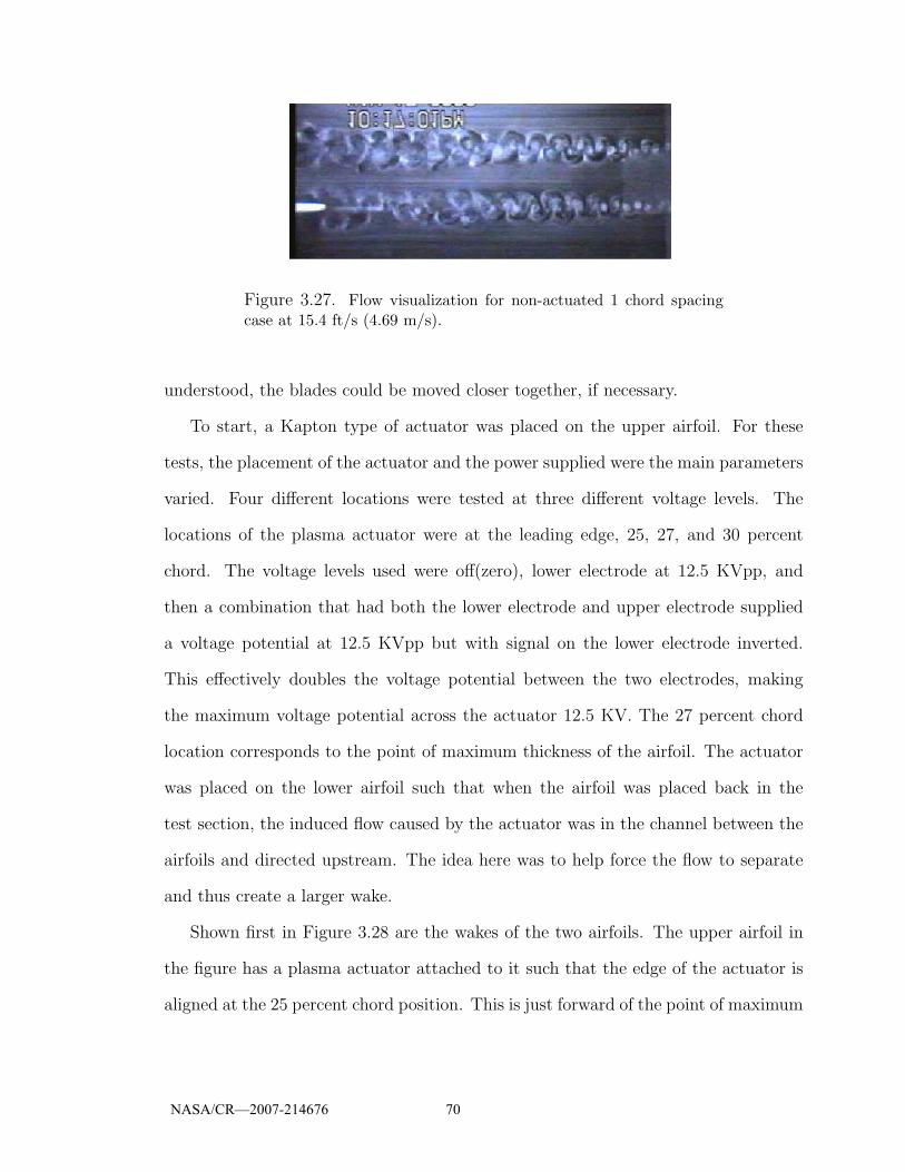
Figure 3.27. Flow visualization for non-actuated 1 chord spacingcase at 15.4 ft/s (4.69 m/s).
understood, the blades could be moved closer together, if necessary.
To start, a Kapton type of actuator was placed on the upper airfoil. For these
tests, the placement of the actuator and the power supplied were the main parameters
varied. Four different locations were tested at three different voltage levels. The
locations of the plasma actuator were at the leading edge, 25, 27, and 30 percent
chord. The voltage levels used were off(zero), lower electrode at 12.5 KVpp, and
then a combination that had both the lower electrode and upper electrode supplied
a voltage potential at 12.5 KVpp but with signal on the lower electrode inverted.
This effectively doubles the voltage potential between the two electrodes, making
the maximum voltage potential across the actuator 12.5 KV. The 27 percent chord
location corresponds to the point of maximum thickness of the airfoil. The actuator
was placed on the lower airfoil such that when the airfoil was placed back in the
test section, the induced flow caused by the actuator was in the channel between the
airfoils and directed upstream. The idea here was to help force the flow to separate
and thus create a larger wake.
Shown first in Figure 3.28 are the wakes of the two airfoils. The upper airfoil in
the figure has a plasma actuator attached to it such that the edge of the actuator is
aligned at the 25 percent chord position. This is just forward of the point of maximum
NASA/CR—2007-214676 70

thickness. To help illustrate the effect of the actuator, Figure 3.28-A shows the wakes
with the actuator ‘off’, and Figure 3.28-B shows the wakes when the actuator is
turned ‘on’ at the 6.3 KV voltage potential. That is, one electrode is being supplied
power and the other is grounded. It is apparent that there is no real distinguishable
effect by the actuator on the flow.
A: Actuator ‘off’ B: Actuator ‘on’ (upper airfoil)
Figure 3.28. Comparison with actuator at 25 percent chord, forward of the point ofmaximum thickness of airfoil, at 6.3 KV potential.
The power was then increased and these results are shown in 3.29. Again with
sub-figure A being the ‘off’ case and sub-figure B being the ‘on’ case. In Figure 3.29-B
there appears to be some effect by the actuator. It can be seen by close observation
of the edges of the upper wake, in approximately the middle of the image, that the
vortical structure of the wake has been broken up some. This is in contrast to the ‘off’
case were the half moon shapes are still very distinguishable along the wake edges.
A: Actuator ‘off’ B: Actuator ‘on’ (upper airfoil)
Figure 3.29. Comparison with actuator at 25 percent chord, forward of the point ofmaximum thickness of airfoil, at 12.5 KV potential.
NASA/CR—2007-214676 71
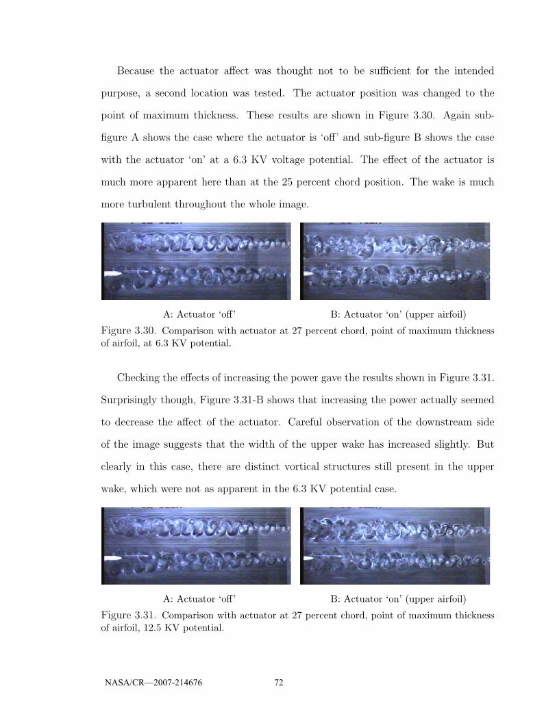
Because the actuator affect was thought not to be sufficient for the intended
purpose, a second location was tested. The actuator position was changed to the
point of maximum thickness. These results are shown in Figure 3.30. Again sub-
figure A shows the case where the actuator is ‘off’ and sub-figure B shows the case
with the actuator ‘on’ at a 6.3 KV voltage potential. The effect of the actuator is
much more apparent here than at the 25 percent chord position. The wake is much
more turbulent throughout the whole image.
A: Actuator ‘off’ B: Actuator ‘on’ (upper airfoil)
Figure 3.30. Comparison with actuator at 27 percent chord, point of maximum thicknessof airfoil, at 6.3 KV potential.
Checking the effects of increasing the power gave the results shown in Figure 3.31.
Surprisingly though, Figure 3.31-B shows that increasing the power actually seemed
to decrease the affect of the actuator. Careful observation of the downstream side
of the image suggests that the width of the upper wake has increased slightly. But
clearly in this case, there are distinct vortical structures still present in the upper
wake, which were not as apparent in the 6.3 KV potential case.
A: Actuator ‘off’ B: Actuator ‘on’ (upper airfoil)
Figure 3.31. Comparison with actuator at 27 percent chord, point of maximum thicknessof airfoil, 12.5 KV potential.
NASA/CR—2007-214676 72
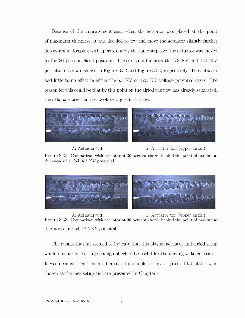
Because of the improvement seen when the actuator was placed at the point
of maximum thickness, it was decided to try and move the actuator slightly further
downstream. Keeping with approximately the same step size, the actuator was moved
to the 30 percent chord position. These results for both the 6.3 KV and 12.5 KV
potential cases are shown in Figure 3.32 and Figure 3.33, respectively. The actuator
had little to no effect in either the 6.3 KV or 12.5 KV voltage potential cases. The
reason for this could be that by this point on the airfoil the flow has already separated,
thus the actuator can not work to separate the flow.
A: Actuator ‘off’ B: Actuator ‘on’ (upper airfoil)
Figure 3.32. Comparison with actuator at 30 percent chord, behind the point of maximumthickness of airfoil, 6.3 KV potential.
A: Actuator ‘off’ B: Actuator ‘on’ (upper airfoil)Figure 3.33. Comparison with actuator at 30 percent chord, behind the point of maximum
thickness of airfoil, 12.5 KV potential.
The results thus far seemed to indicate that this plasma actuator and airfoil setup
would not produce a large enough affect to be useful for the moving-wake generator.
It was decided then that a different setup should be investigated. Flat plates were
chosen as the new setup and are presented in Chapter 4.
NASA/CR—2007-214676 73
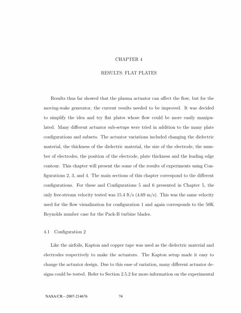
CHAPTER 4
RESULTS: FLAT PLATES
Results thus far showed that the plasma actuator can affect the flow, but for the
moving-wake generator, the current results needed to be improved. It was decided
to simplify the idea and try flat plates whose flow could be more easily manipu-
lated. Many different actuator sub-setups were tried in addition to the many plate
configurations and subsets. The actuator variations included changing the dielectric
material, the thickness of the dielectric material, the size of the electrode, the num-
ber of electrodes, the position of the electrode, plate thickness and the leading edge
contour. This chapter will present the some of the results of experiments using Con-
figurations 2, 3, and 4. The main sections of this chapter correspond to the different
configurations. For these and Configurations 5 and 6 presented in Chapter 5, the
only free-stream velocity tested was 15.4 ft/s (4.69 m/s). This was the same velocity
used for the flow visualization for configuration 1 and again corresponds to the 50K
Reynolds number case for the Pack-B turbine blades.
4.1 Configuration 2
Like the airfoils, Kapton and copper tape was used as the dielectric material and
electrodes respectively to make the actuators. The Kapton setup made it easy to
change the actuator design. Due to this ease of variation, many different actuator de-
signs could be tested. Refer to Section 2.5.2 for more information on the experimental
NASA/CR—2007-214676 74

setup. The only investigations performed on Configuration 2 used flow visualization.
This was due to problems encountered with the longevity of the Kapton actuators.
Quantitative measurements using a hot-wire could not be completed before the actu-
ator failed. The flat plates were first tried at a zero degree angle of attack and then
at other various angles. A summary of the flow visualization results are presented in
the following subsections.
4.1.1 Zero Angle of Attack
For the application of the moving-wake generator, it was thought to try and
minimize the turbulence caused by the apparatus itself. In other words, the amount
of blockage and effect on the flow without the plasma actuators running should be
minimized as much as possible. To do this, the two plates were set side-by-side, at a
zero degree angle of attack, thus creating a channel between the two plates.
The first experiments had an actuator setup that used a single actuator whose
upper electrode was positioned 0.125 in. (3.18 mm) from the leading edge of the
plate. In terms of the chord, this was at the 1/16th chord location. Also, the electrodes
themselves were both 0.125 in. (3.18 mm) wide. The orientation was chosen such
that the flow induced by the actuator was in the channel of the plates and directed
upstream. This was chosen to try to separate the flow and cause a blockage in the
channel between the plates that would impede the flow entering the channel. This
would in turn cause a large velocity deficit in the wake profiles downstream of the
channel, basically making the two plates and channel act like a single bluff body.
In these tests, the lower electrode was supplied a 5.0 KHz triangular waveform of
up to 3.8 KVpp and the upper electrode was grounded, thus making the highest
voltage potential across the actuator 1.9 KV. This setup did not have any noticeable
effect on the flow. Another attempt was made having the actuator at the mid-
NASA/CR—2007-214676 75

chord location but again without positive results. All these tests were done at 1/2
chord and 1/4 chord plate spacings. Based on the the immediate feedback from the
flow visualizations, most of these tests were not documented because there was no
noticeable change in the flow.
After the previous tries, some attempts were made at using a four actuator array,
with the same intention of blocking the flow from entering the channel. The actuators
were arranged so that there was an electrode positioned at the 1/16th, 1/4, 1/2, and
3/4 chord locations, again using the 0.125 in. (3.18 mm) width electrodes. This
case also had the lower electrodes grounded and the upper electrodes supplied the
3.8 KVpp, 5.0 KHz triangle wave. The 1/4 chord plate spacing case is shown in
Figure 4.1. In the figure, the upper plate is the plate with the plasma actuators.
It is apparent from this that the actuators had little to no effect. This setup was
tried at 1/4 chord and 3/8 chord plate spacings with similar results. Following these
tests, a different set of transformers were used that had more windings, thus a voltage
higher gain, which would yield a higher voltage potential across the plasma actuators’
electrodes. Doing this gave some improvement but still not enough, so another set of
four actuators were added to the neighboring plate.
A: Actuator off B: Actuator on (lower plate)
Figure 4.1. Four actuators with 1/2 chord plate spacing at a maximum voltage potentialof 1.9 KV.
Keeping with the idea of trying to deter the flow from entering the channel, the
same four actuator array was added to the neighboring plate such that both arrays
were in the channel between the plates and inducing a flow upstream. Shown in
NASA/CR—2007-214676 76

Figure 4.2 are the results of these tests at 1/4 chord plate spacing. Figure 4.2-A, is
the case of having the actuators ‘off’, Figure 4.2-B is the case of having the actuators
on the upper plate in the figures ‘on’, and lastly, Figure 4.2-C shows the result of
having the actuators of both plates ‘on’ at the same time. Note that the wakes shown
in the pictures are not turned or shifted by the plates. The reason the wakes do not
appear to follow the plates is because the camera and mirror were not perfectly in
line with the center of the test section. The plates edges seen in the picture are at
the bottom of the test section, and the smoke is in the middle of the test section, but
due to the angle of the camera, they appear to not line up. In this case, a 13.6 KVpp
triangle wave was supplied to the lower electrode(s), making the maximum voltage
potential across the actuator 6.8 KV. Though not very much, these images do show
some effect of the actuator, but more affect was needed so a completely different
approach was tried.
A: Actuator off B: Actuator on (lower plate)
C: Actuators on (both plates)
Figure 4.2. Four actuators with 1/4 chord plate spacing at a maxi-mum voltage potential of 6.8 KV.
NASA/CR—2007-214676 77
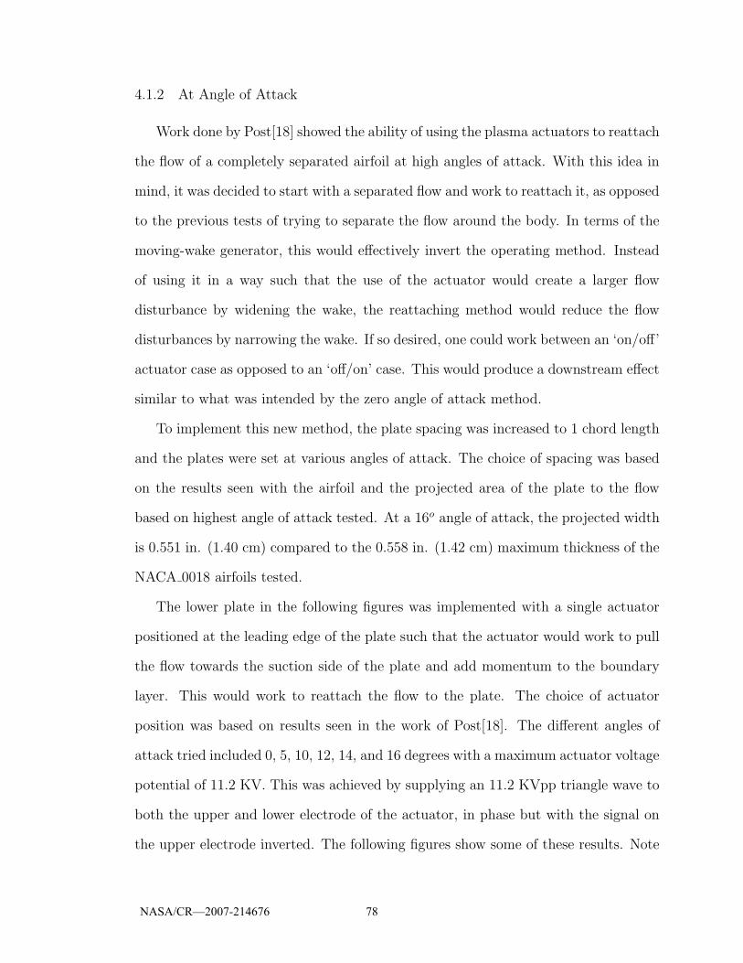
4.1.2 At Angle of Attack
Work done by Post[18] showed the ability of using the plasma actuators to reattach
the flow of a completely separated airfoil at high angles of attack. With this idea in
mind, it was decided to start with a separated flow and work to reattach it, as opposed
to the previous tests of trying to separate the flow around the body. In terms of the
moving-wake generator, this would effectively invert the operating method. Instead
of using it in a way such that the use of the actuator would create a larger flow
disturbance by widening the wake, the reattaching method would reduce the flow
disturbances by narrowing the wake. If so desired, one could work between an ‘on/off’
actuator case as opposed to an ‘off/on’ case. This would produce a downstream effect
similar to what was intended by the zero angle of attack method.
To implement this new method, the plate spacing was increased to 1 chord length
and the plates were set at various angles of attack. The choice of spacing was based
on the results seen with the airfoil and the projected area of the plate to the flow
based on highest angle of attack tested. At a 16o angle of attack, the projected width
is 0.551 in. (1.40 cm) compared to the 0.558 in. (1.42 cm) maximum thickness of the
NACA 0018 airfoils tested.
The lower plate in the following figures was implemented with a single actuator
positioned at the leading edge of the plate such that the actuator would work to pull
the flow towards the suction side of the plate and add momentum to the boundary
layer. This would work to reattach the flow to the plate. The choice of actuator
position was based on results seen in the work of Post[18]. The different angles of
attack tried included 0, 5, 10, 12, 14, and 16 degrees with a maximum actuator voltage
potential of 11.2 KV. This was achieved by supplying an 11.2 KVpp triangle wave to
both the upper and lower electrode of the actuator, in phase but with the signal on
the upper electrode inverted. The following figures show some of these results. Note
NASA/CR—2007-214676 78

that in the following figures, the lower plate is the one with the plasma actuator.
Careful observation of the wakes behind the lower plate in Figure 4.3 show that
there was only a slight narrowing of the wake. As discussed in Section 2.6, the
appearance that the plates in the figure are not parallel is an optical illusion caused
by the camera/mirror setup. The angle of attack was then increased. As the angle
was increased, the actuator effect became more noticeable.
A: Actuator off B: Actuator on (lower plate)
Figure 4.3. One actuator at leading edge of plate at zero degrees, 11.2 KV voltage potential,and 1 chord plate spacing.
In the 5o angle of attack case shown in Figure 4.4, the effect of the actuator is
much more noticeable. The wake behind the lower plate is more narrow than the
upper wake and looks more uniform. This effect is even more noticeable in the 10o
case.
A: Actuator off B: Actuator on (lower plate)
Figure 4.4. One actuator at leading edge of plate at 5o, 11.2 KV voltage potential, and 1chord plate spacing.
Again, these images need to be viewed with some caution. In Figure 4.5 the
lower plate looks like it is at close to zero angle of attack but careful comparison of
NASA/CR—2007-214676 79

A: Actuator off B: Actuator on (lower plate)
Figure 4.5. One actuator at leading edge of plate at 10o, 11.2 KV voltage potential, and 1chord plate spacing.
the holders at the end of the plates shows that the angle of the two plates is the
same. Sub-figure B clearly shows by the thinning of the wake that the flow is being
reattached to the plate.
The last case shown is that of the greatest angle investigated. This angle was
16o. The result is shown in Figure 4.6. Again, it is clear that the actuator helps to
reattach the flow subsequently reducing the width and unsteadiness of the wake.
A: Actuator off B: Actuator on (lower plate)
Figure 4.6. One actuator at leading edge of plate 16o, 11.2 KV voltage potential and 1chord plate spacing.
As a side note, viewing the flow visualization for the 10 and 16 degree angles of
attack, the thinning of the wake of the actuated blade appeared to affect the wake of
the unactuated blade. More than likely, there was some degree of communication or
cross-forcing of the wake structures that was reduced when the strength, or width, of
the one wake was reduced by the actuator.
The previous results were very promising and sufficient to return to the hot-wire
NASA/CR—2007-214676 80

measurements to quantitatively investigate the wakes. The stream profiles for these
cases however proved to be difficult to obtain. As mentioned in Section 2.3, there
were long times associated with taking the individual wake profiles. The individual
profiles took close to 10 minutes, thus making the full set of stream profiles take close
to two hours to perform. Half of this time the plasma actuator would be in use. The
actuators lasted anywhere from around 5 to 20 minutes, so the full set of profiles
could not be completed before the actuator burned out. Because each actuator was
hand made, it was thought that they would be too inconsistent to replace after each
individual wake profile to complete the set of stream profiles. Different thicknesses
of Kapton were tried to increase durability and overcome this problem. Up to three
layers of 2 mil (0.051 mm) were tried, which was used for the flow visualization images
previously shown. Also a single layer of 5 mil (0.127 mm) Kapton was tried.
Though increasing the Kapton thickness in some cases helped, other problems with
the pliability of the thicker Kapton were sometimes encountered. Adhesive problems
with the copper tape also developed. Using a flat plate and orienting the actuator
on the leading edge caused a very sharp turn of the copper tape over the edge of
the plate. When used for long periods of time the adhesive would heat up and start
to fail. This would allow the copper tape to start to separate from the Kapton and
cause the actuator to fail. Because it was not possible to complete the measurements
needed to validate the setups that, based on the flow visualization, were working the
implementation of these for the moving-wake generator did not seem feasible. Thus
a new approach was needed. The new approached used actuators made from factory
copper clad, FR4 material printed circuit boards.
NASA/CR—2007-214676 81
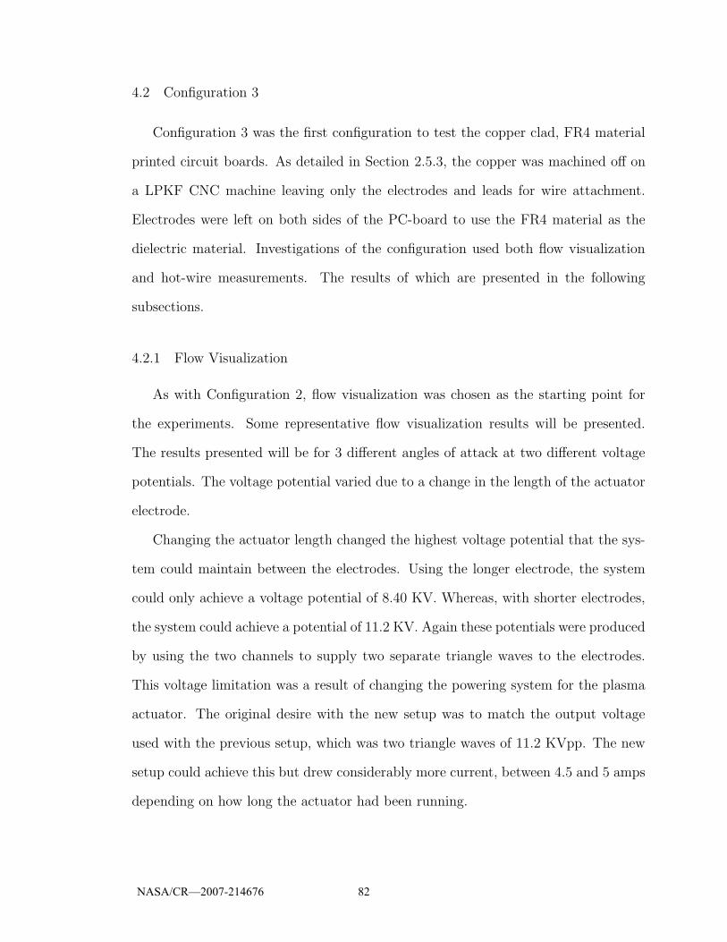
4.2 Configuration 3
Configuration 3 was the first configuration to test the copper clad, FR4 material
printed circuit boards. As detailed in Section 2.5.3, the copper was machined off on
a LPKF CNC machine leaving only the electrodes and leads for wire attachment.
Electrodes were left on both sides of the PC-board to use the FR4 material as the
dielectric material. Investigations of the configuration used both flow visualization
and hot-wire measurements. The results of which are presented in the following
subsections.
4.2.1 Flow Visualization
As with Configuration 2, flow visualization was chosen as the starting point for
the experiments. Some representative flow visualization results will be presented.
The results presented will be for 3 different angles of attack at two different voltage
potentials. The voltage potential varied due to a change in the length of the actuator
electrode.
Changing the actuator length changed the highest voltage potential that the sys-
tem could maintain between the electrodes. Using the longer electrode, the system
could only achieve a voltage potential of 8.40 KV. Whereas, with shorter electrodes,
the system could achieve a potential of 11.2 KV. Again these potentials were produced
by using the two channels to supply two separate triangle waves to the electrodes.
This voltage limitation was a result of changing the powering system for the plasma
actuator. The original desire with the new setup was to match the output voltage
used with the previous setup, which was two triangle waves of 11.2 KVpp. The new
setup could achieve this but drew considerably more current, between 4.5 and 5 amps
depending on how long the actuator had been running.
NASA/CR—2007-214676 82

Upon switching to the PC type actuator, and seeing the initial flow visualization
results, it was decided to return to the original idea of starting with an attached flow
and using the actuator to separate it. To this end, the angle of attack was reduced, as
compared to the previous tests, to range from -3 to -7 degrees. Positive angles of these
were also tried but were found to be less effective. The main reason for the choice of
the negative angles was to have the upper plate be the one with the actuator and stay
with the concept of separating the flow. Because of the non-symmetric leading edge,
to have the plates at a positive angle of attack, relative to the flow, they would have
to be flipped over and swapped. Recall from Section 2.5.3 that in this configuration,
since the plate itself is being used as the dielectric material, plasma will form on both
sides of the plate, thus inducing two flows, one upstream and one downstream. As
with the airfoils and the previous flat plates, the upstream flow induced by the plasma
was in the channel created by the two plates, thus again working to block the main
flow from entering the channel.
Recall from Section 2.4 that the active edge of the plasma actuator of the PC
design type could not be manufactured on the leading edge of the plate. Choosing
electrode widths of 1 in. (2.54 cm), forced the active edge of the plasma actuator
to be moved to the mid-chord location. One experiment was done to see if changing
the location of the active edge of the electrode would be beneficial. To do this, what
is considered the lower electrode was shortened to 0.50 in. (1.27 cm). Doing this
shifted the active edge to the 1/4 chord location. The end result was not as effective
as having the active edge at the mid-chord location. Part of the reason for this is
the detrimental effect of shortening the width of the lower electrode[17]. So the 1.0
in. (2.54 cm) actuator width was returned to and was used for all of the following
results.
NASA/CR—2007-214676 83

As before, shown in Figure 4.7 is an ‘off/on’ comparison. The case shown is the
negative −3o case with an 8.0 x 1.0 in. (20.3 x 2.54 cm) lower electrode. Comparing
the wakes of the upper plate in sub-figure A and B shows that there is an effect of
the actuator. As opposed to the previous effects of narrowing the wake, the wake of
the upper plate in this case is distinctly wider.
A: Actuator off B: Actuator on (upper plate)
Figure 4.7. −3o, 1 chord plate spacing, and 8.4 KV maximum voltage potential case.
The −5o case shown in Figure 4.8 shows some widening of the wake but also some
large unsteady regions. These regions seem to distort the wake. On average, these
distortions could show up as an even wider wake in a mean hot-wire profile.
A: Actuator off B: Actuator on (upper plate)
Figure 4.8. −5o, 1 chord plate spacing, and 8.4 KV maximum voltage potential case.
This last case shows some even more unsteadiness in the upper wake. In Figure
4.9 it can be seen that the amount of interaction between the two wakes is increased
in the ‘on’ case in addition to the unsteadiness of the wake.
Repeating the three previously shown angles of attack with the 4.75 in (12.07
cm) electrode gives the following results. For the −3o case, Figure 4.10 showed an
even greater effect than the previously seen −3o case with the lower voltage potential
NASA/CR—2007-214676 84
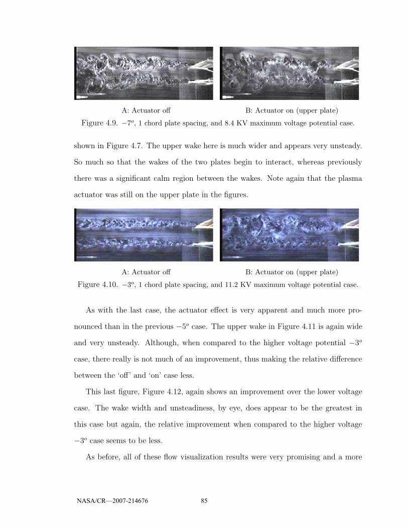
A: Actuator off B: Actuator on (upper plate)
Figure 4.9. −7o, 1 chord plate spacing, and 8.4 KV maximum voltage potential case.
shown in Figure 4.7. The upper wake here is much wider and appears very unsteady.
So much so that the wakes of the two plates begin to interact, whereas previously
there was a significant calm region between the wakes. Note again that the plasma
actuator was still on the upper plate in the figures.
A: Actuator off B: Actuator on (upper plate)
Figure 4.10. −3o, 1 chord plate spacing, and 11.2 KV maximum voltage potential case.
As with the last case, the actuator effect is very apparent and much more pro-
nounced than in the previous −5o case. The upper wake in Figure 4.11 is again wide
and very unsteady. Although, when compared to the higher voltage potential −3o
case, there really is not much of an improvement, thus making the relative difference
between the ‘off’ and ‘on’ case less.
This last figure, Figure 4.12, again shows an improvement over the lower voltage
case. The wake width and unsteadiness, by eye, does appear to be the greatest in
this case but again, the relative improvement when compared to the higher voltage
−3o case seems to be less.
As before, all of these flow visualization results were very promising and a more
NASA/CR—2007-214676 85
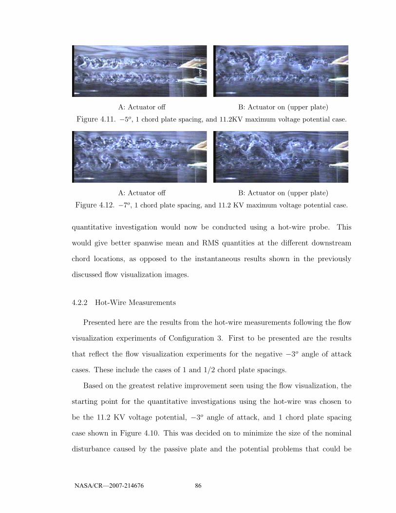
A: Actuator off B: Actuator on (upper plate)
Figure 4.11. −5o, 1 chord plate spacing, and 11.2KV maximum voltage potential case.
A: Actuator off B: Actuator on (upper plate)
Figure 4.12. −7o, 1 chord plate spacing, and 11.2 KV maximum voltage potential case.
quantitative investigation would now be conducted using a hot-wire probe. This
would give better spanwise mean and RMS quantities at the different downstream
chord locations, as opposed to the instantaneous results shown in the previously
discussed flow visualization images.
4.2.2 Hot-Wire Measurements
Presented here are the results from the hot-wire measurements following the flow
visualization experiments of Configuration 3. First to be presented are the results
that reflect the flow visualization experiments for the negative −3o angle of attack
cases. These include the cases of 1 and 1/2 chord plate spacings.
Based on the greatest relative improvement seen using the flow visualization, the
starting point for the quantitative investigations using the hot-wire was chosen to
be the 11.2 KV voltage potential, −3o angle of attack, and 1 chord plate spacing
case shown in Figure 4.10. This was decided on to minimize the size of the nominal
disturbance caused by the passive plate and the potential problems that could be
NASA/CR—2007-214676 86
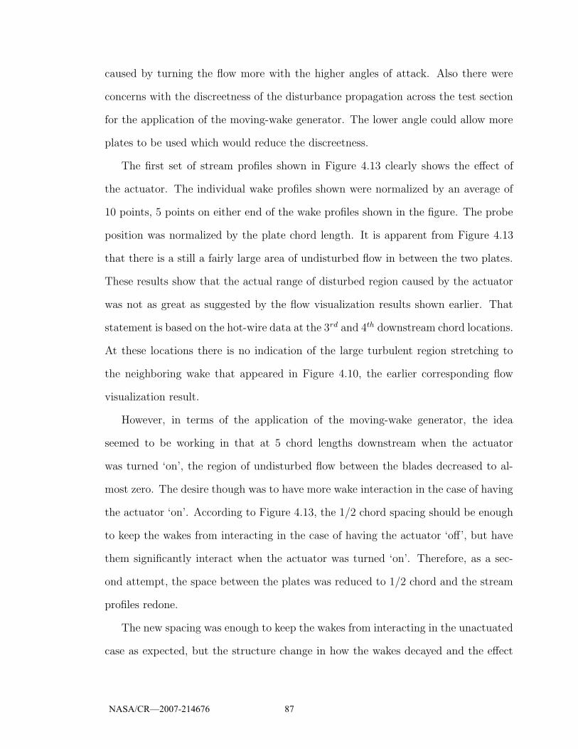
caused by turning the flow more with the higher angles of attack. Also there were
concerns with the discreetness of the disturbance propagation across the test section
for the application of the moving-wake generator. The lower angle could allow more
plates to be used which would reduce the discreetness.
The first set of stream profiles shown in Figure 4.13 clearly shows the effect of
the actuator. The individual wake profiles shown were normalized by an average of
10 points, 5 points on either end of the wake profiles shown in the figure. The probe
position was normalized by the plate chord length. It is apparent from Figure 4.13
that there is a still a fairly large area of undisturbed flow in between the two plates.
These results show that the actual range of disturbed region caused by the actuator
was not as great as suggested by the flow visualization results shown earlier. That
statement is based on the hot-wire data at the 3rd and 4th downstream chord locations.
At these locations there is no indication of the large turbulent region stretching to
the neighboring wake that appeared in Figure 4.10, the earlier corresponding flow
visualization result.
However, in terms of the application of the moving-wake generator, the idea
seemed to be working in that at 5 chord lengths downstream when the actuator
was turned ‘on’, the region of undisturbed flow between the blades decreased to al-
most zero. The desire though was to have more wake interaction in the case of having
the actuator ‘on’. According to Figure 4.13, the 1/2 chord spacing should be enough
to keep the wakes from interacting in the case of having the actuator ‘off’, but have
them significantly interact when the actuator was turned ‘on’. Therefore, as a sec-
ond attempt, the space between the plates was reduced to 1/2 chord and the stream
profiles redone.
The new spacing was enough to keep the wakes from interacting in the unactuated
case as expected, but the structure change in how the wakes decayed and the effect
NASA/CR—2007-214676 87
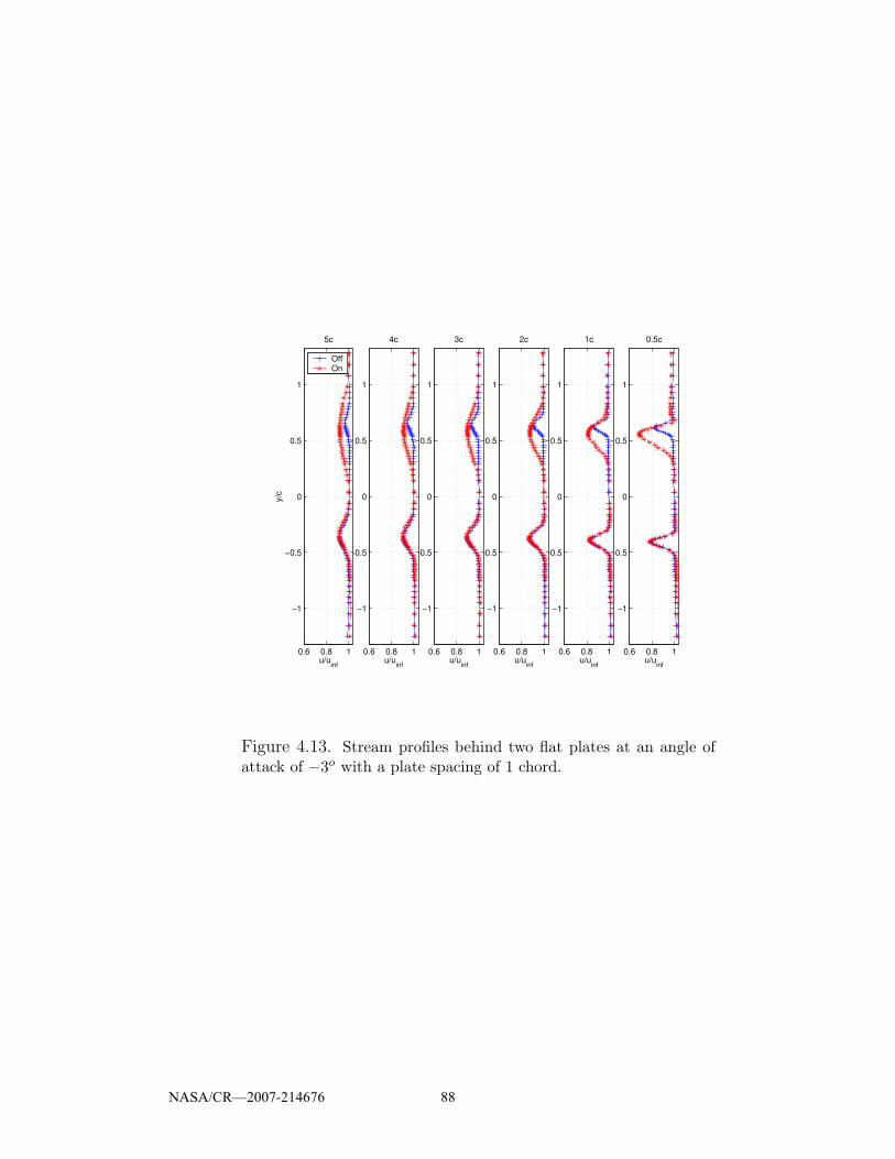
0.6 0.8 1
−1
−0.5
0
0.5
1
u/uinf
0.5c
0.6 0.8 1
−1
−0.5
0
0.5
1
u/uinf
1c
0.6 0.8 1
−1
−0.5
0
0.5
1
u/uinf
2c
0.6 0.8 1
−1
−0.5
0
0.5
1
u/uinf
3c
0.6 0.8 1
−1
−0.5
0
0.5
1
u/uinf
4c
0.6 0.8 1
−1
−0.5
0
0.5
1
u/uinf
y/c
5c
OffOn
Figure 4.13. Stream profiles behind two flat plates at an angle ofattack of −3o with a plate spacing of 1 chord.
NASA/CR—2007-214676 88
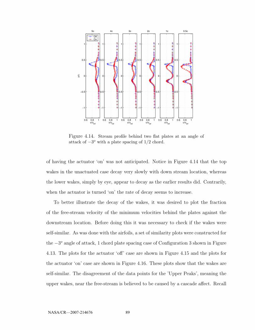
0.6 0.8 1
−1
−0.5
0
0.5
1
u/uinf
0.5c
0.6 0.8 1
−1
−0.5
0
0.5
1
u/uinf
1c
0.6 0.8 1
−1
−0.5
0
0.5
1
u/uinf
2c
0.6 0.8 1
−1
−0.5
0
0.5
1
u/uinf
3c
0.6 0.8 1
−1
−0.5
0
0.5
1
u/uinf
4c
0.6 0.8 1
−1
−0.5
0
0.5
1
u/uinf
y/c
5c
OffOn
Figure 4.14. Stream profile behind two flat plates at an angle ofattack of −3o with a plate spacing of 1/2 chord.
of having the actuator ‘on’ was not anticipated. Notice in Figure 4.14 that the top
wakes in the unactuated case decay very slowly with down stream location, whereas
the lower wakes, simply by eye, appear to decay as the earlier results did. Contrarily,
when the actuator is turned ‘on’ the rate of decay seems to increase.
To better illustrate the decay of the wakes, it was desired to plot the fraction
of the free-stream velocity of the minimum velocities behind the plates against the
downstream location. Before doing this it was necessary to check if the wakes were
self-similar. As was done with the airfoils, a set of similarity plots were constructed for
the −3o angle of attack, 1 chord plate spacing case of Configuration 3 shown in Figure
4.13. The plots for the actuator ‘off’ case are shown in Figure 4.15 and the plots for
the actuator ‘on’ case are shown in Figure 4.16. These plots show that the wakes are
self-similar. The disagreement of the data points for the ’Upper Peaks’, meaning the
upper wakes, near the free-stream is believed to be caused by a cascade affect. Recall
NASA/CR—2007-214676 89
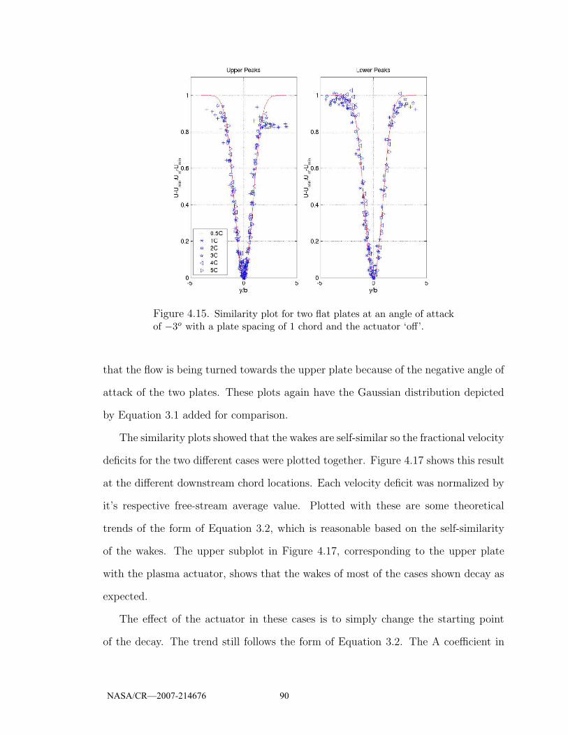
Figure 4.15. Similarity plot for two flat plates at an angle of attackof −3o with a plate spacing of 1 chord and the actuator ‘off’.
that the flow is being turned towards the upper plate because of the negative angle of
attack of the two plates. These plots again have the Gaussian distribution depicted
by Equation 3.1 added for comparison.
The similarity plots showed that the wakes are self-similar so the fractional velocity
deficits for the two different cases were plotted together. Figure 4.17 shows this result
at the different downstream chord locations. Each velocity deficit was normalized by
it’s respective free-stream average value. Plotted with these are some theoretical
trends of the form of Equation 3.2, which is reasonable based on the self-similarity
of the wakes. The upper subplot in Figure 4.17, corresponding to the upper plate
with the plasma actuator, shows that the wakes of most of the cases shown decay as
expected.
The effect of the actuator in these cases is to simply change the starting point
of the decay. The trend still follows the form of Equation 3.2. The A coefficient in
NASA/CR—2007-214676 90

Figure 4.16. Similarity plot for two flat plates at an angle of attackof −3o with a plate spacing of 1 chord and the actuator ‘on’.
Equation 3.2 is less for the cases with the actuator ‘on’.
The lower subplot in Figure 4.17, corresponds to the unactuated plate. This shows
that the actuator had little effect on the wakes behind the lower plate in all of the
cases.
The only case that does not follow the trend is the 1/2 chord plate spacing with
the actuator ‘off’. This seems to imply a cascade effect, caused by the turning of
the flow because only the upper wake is being effected. Recall that the flow is being
directed towards the upper plate because of the angle of attack of the plates. The use
of the actuator seems to eliminate this cascade effect because the decay trend closely
matches the 1 chord plate spacing case with the actuator ‘on’.
The pressure transducer happened to use a carrier frequency of 5.0 KHz, the same
frequency being used for the plasma actuator. The pressure transducer readings, while
the actuator was in use, were affected. It was decided to try a slightly higher frequency
NASA/CR—2007-214676 91
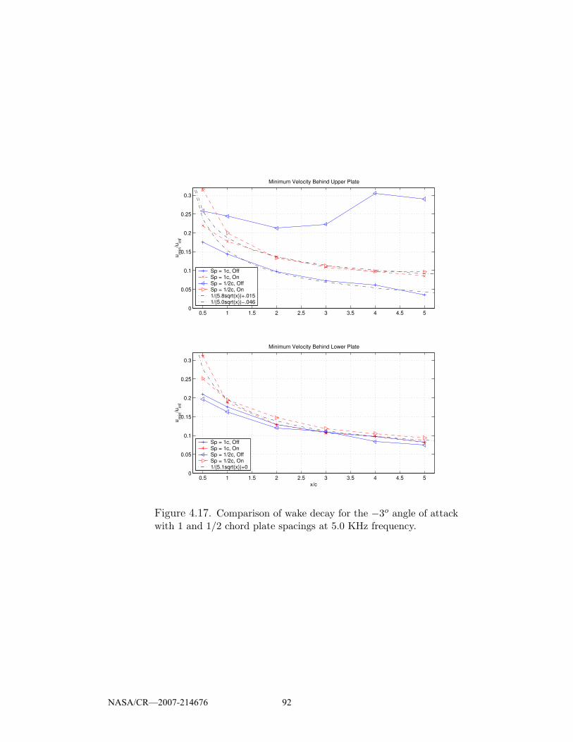
0.5 1 1.5 2 2.5 3 3.5 4 4.5 50
0.05
0.1
0.15
0.2
0.25
0.3
u min
/uin
fMinimum Velocity Behind Upper Plate
Sp = 1c, OffSp = 1c, OnSp = 1/2c, OffSp = 1/2c, On1/(5.8sqrt(x))+.0151/(5.0sqrt(x))−.046
0.5 1 1.5 2 2.5 3 3.5 4 4.5 50
0.05
0.1
0.15
0.2
0.25
0.3
x/c
u min
/uin
f
Minimum Velocity Behind Lower Plate
Sp = 1c, OffSp = 1c, OnSp = 1/2c, OffSp = 1/2c, On1/(5.1sqrt(x))+0
Figure 4.17. Comparison of wake decay for the −3o angle of attackwith 1 and 1/2 chord plate spacings at 5.0 KHz frequency.
NASA/CR—2007-214676 92
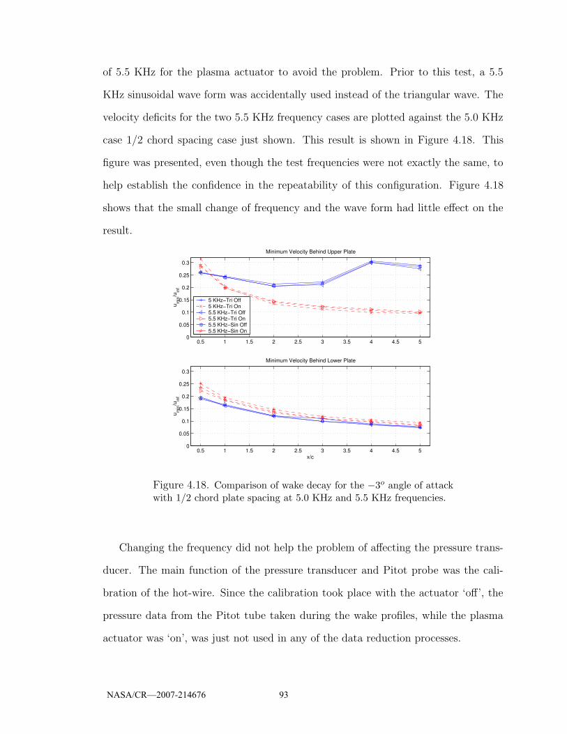
of 5.5 KHz for the plasma actuator to avoid the problem. Prior to this test, a 5.5
KHz sinusoidal wave form was accidentally used instead of the triangular wave. The
velocity deficits for the two 5.5 KHz frequency cases are plotted against the 5.0 KHz
case 1/2 chord spacing case just shown. This result is shown in Figure 4.18. This
figure was presented, even though the test frequencies were not exactly the same, to
help establish the confidence in the repeatability of this configuration. Figure 4.18
shows that the small change of frequency and the wave form had little effect on the
result.
0.5 1 1.5 2 2.5 3 3.5 4 4.5 50
0.05
0.1
0.15
0.2
0.25
0.3
u min
/uin
f
Minimum Velocity Behind Upper Plate
5 KHz−Tri Off5 KHz−Tri On5.5 KHz−Tri Off5.5 KHz−Tri On5.5 KHz−Sin Off5.5 KHz−Sin On
0.5 1 1.5 2 2.5 3 3.5 4 4.5 50
0.05
0.1
0.15
0.2
0.25
0.3
x/c
u min
/uin
f
Minimum Velocity Behind Lower Plate
Figure 4.18. Comparison of wake decay for the −3o angle of attackwith 1/2 chord plate spacing at 5.0 KHz and 5.5 KHz frequencies.
Changing the frequency did not help the problem of affecting the pressure trans-
ducer. The main function of the pressure transducer and Pitot probe was the cali-
bration of the hot-wire. Since the calibration took place with the actuator ‘off’, the
pressure data from the Pitot tube taken during the wake profiles, while the plasma
actuator was ‘on’, was just not used in any of the data reduction processes.
NASA/CR—2007-214676 93

The change made in the setup that had the largest effect was that of the blade
spacing, as shown in Figure 4.17. This suggests that, at least to a point, as the spacing
between the blades decreased, the flow around the plates becomes more sensitive. The
new result promoted the question of what the wakes look like if a third blade was
added. Namely, is what was seen really a spacing or cascade effect and would the
third wake resemble more the current upper wake, the lower wake or neither? To
answer these questions a third blade was added. The addition of the third plate is
what was is referred to as Configuration 4. Upon adding this plate, a new style of
measurements were also performed.
4.3 Configuration 4
With Configuration 4, a new style of tests were started and the flow visualization
experiments ended. The new tests were still wake profiles using the hot-wire and were
what was referred to earlier as power profiles. This is because, instead of varying
the downstream location, as in the case of the stream profiles, the actuator voltage
potential was varied. This new style of testing helped to save time and broaden
the investigation to finding results requiring less power and thus more feasible real
world applications. In addition to time, this method was done in order to reduce
actuator wear due to usage but still obtain workable results. The 5th chord location
was chosen for these experiments because of the actual distance that the 5th chord
location corresponds to, 10.0 in. (25.4 cm). Recall that this distance was the minimal
nominal distance for the first intended application. Only the one chord location was
thought to be necessary for these experiments because the wake structure at the
5th chord location is a result of the upstream conditions, which are affected by the
actuator.
After observing the affect of bringing the plates closer together, it was thought
NASA/CR—2007-214676 94

that the same actuator effect on the wake could be achieved with less power. This
again is also why the the power profiles started.
To this end, the maximum applied voltage was reduced. Shown in 4.19 are the
results for the first set of power profiles on Configuration 4 with the reduced voltages.
These were done at a 1/2 chord plate spacing and an angle of attack of −3o. What
is actually shown in the figure is the magnitude of the velocity deficit, expressed as a
fraction of its local free-stream velocity, behind each plate, plotted against the applied
voltage in KV. As indicated in the figure, the voltage potential was varied from zero to
6.2 KV. To illustrate the advantage of plotting only the minimum, the corresponding
wake profiles are shown in figure 4.20. The later figure has the advantage in that it
more clearly shows the widening of the wake dues to the effect of the actuator but in
general, the figure is difficult to view. As such, the results of the power profiles will
only have the minimum plotted as initially shown in Figure 4.19.
0 1 2 3 4 5 60
0.1
0.2
(uin
f−um
in)/u
inf
Fractional Velocity Deficit Behind Upper Plate
0 1 2 3 4 5 60
0.1
0.2
(uin
f−um
in)/u
inf
Fractional Velocity Deficit Behind Middle Plate (Actuated Plate)
0 1 2 3 4 5 60
0.1
0.2
0.3
Voltage Potential, KV
(uin
f−um
in)/u
inf
Fractional Velocity Deficit Behind Lower Plate
Figure 4.19. Power profile for 3 flat plates at an angle of attack of−3o and 1/2 chord plate spacing.
NASA/CR—2007-214676 95
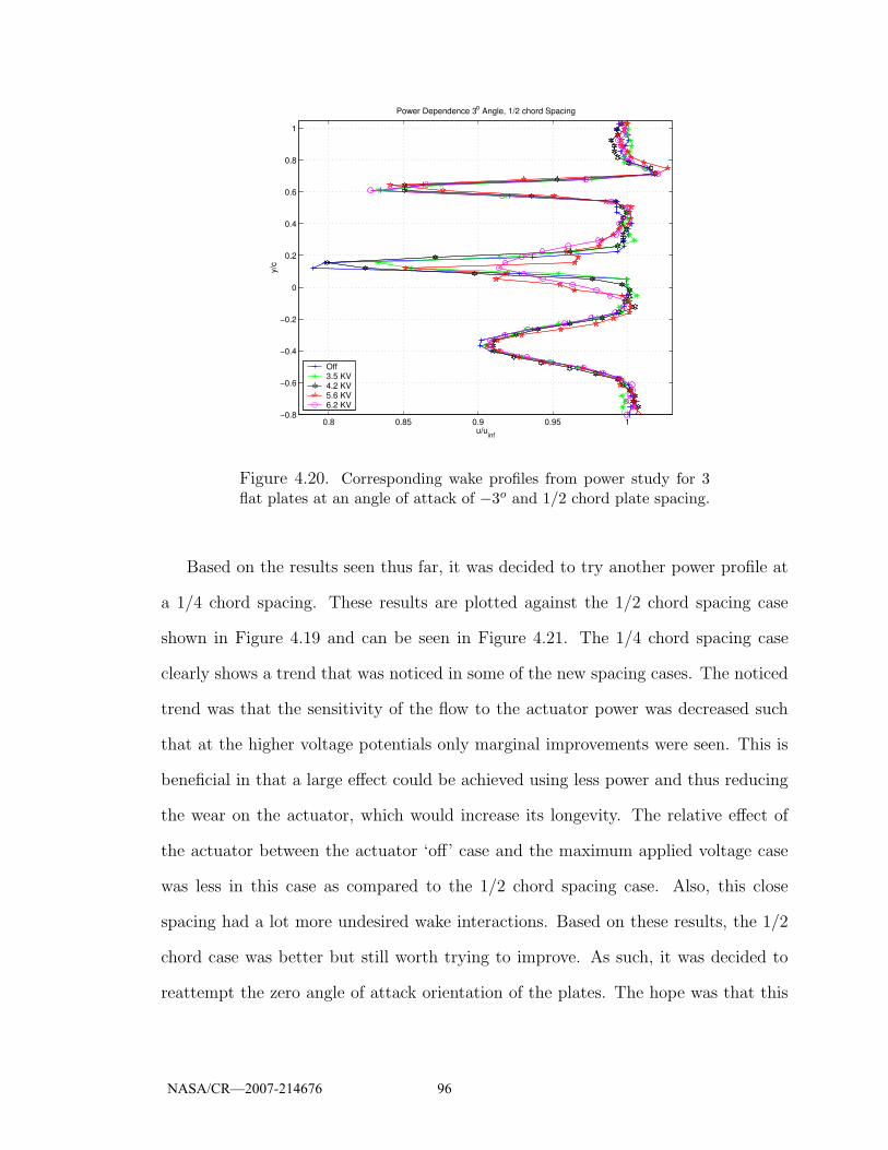
0.8 0.85 0.9 0.95 1−0.8
−0.6
−0.4
−0.2
0
0.2
0.4
0.6
0.8
1
u/uinf
y/c
Power Dependence 3o Angle, 1/2 chord Spacing
Off3.5 KV4.2 KV5.6 KV6.2 KV
Figure 4.20. Corresponding wake profiles from power study for 3flat plates at an angle of attack of −3o and 1/2 chord plate spacing.
Based on the results seen thus far, it was decided to try another power profile at
a 1/4 chord spacing. These results are plotted against the 1/2 chord spacing case
shown in Figure 4.19 and can be seen in Figure 4.21. The 1/4 chord spacing case
clearly shows a trend that was noticed in some of the new spacing cases. The noticed
trend was that the sensitivity of the flow to the actuator power was decreased such
that at the higher voltage potentials only marginal improvements were seen. This is
beneficial in that a large effect could be achieved using less power and thus reducing
the wear on the actuator, which would increase its longevity. The relative effect of
the actuator between the actuator ‘off’ case and the maximum applied voltage case
was less in this case as compared to the 1/2 chord spacing case. Also, this close
spacing had a lot more undesired wake interactions. Based on these results, the 1/2
chord case was better but still worth trying to improve. As such, it was decided to
reattempt the zero angle of attack orientation of the plates. The hope was that this
NASA/CR—2007-214676 96
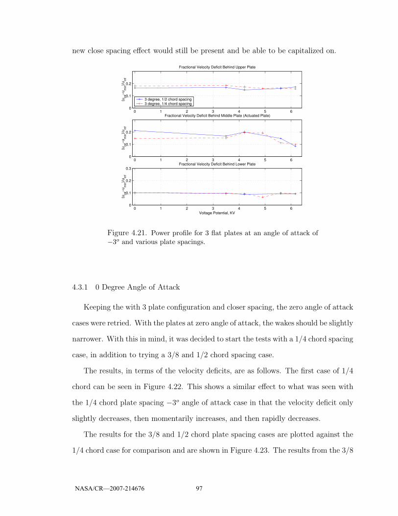
new close spacing effect would still be present and be able to be capitalized on.
0 1 2 3 4 5 60
0.1
0.2
(uin
f−um
in)/u
inf
Fractional Velocity Deficit Behind Upper Plate
3 degree, 1/2 chord spacing3 degree, 1/4 chord spacing
0 1 2 3 4 5 60
0.1
0.2
(uin
f−um
in)/u
inf
Fractional Velocity Deficit Behind Middle Plate (Actuated Plate)
0 1 2 3 4 5 60
0.1
0.2
0.3
Voltage Potential, KV
(uin
f−um
in)/u
inf
Fractional Velocity Deficit Behind Lower Plate
Figure 4.21. Power profile for 3 flat plates at an angle of attack of−3o and various plate spacings.
4.3.1 0 Degree Angle of Attack
Keeping the with 3 plate configuration and closer spacing, the zero angle of attack
cases were retried. With the plates at zero angle of attack, the wakes should be slightly
narrower. With this in mind, it was decided to start the tests with a 1/4 chord spacing
case, in addition to trying a 3/8 and 1/2 chord spacing case.
The results, in terms of the velocity deficits, are as follows. The first case of 1/4
chord can be seen in Figure 4.22. This shows a similar effect to what was seen with
the 1/4 chord plate spacing −3o angle of attack case in that the velocity deficit only
slightly decreases, then momentarily increases, and then rapidly decreases.
The results for the 3/8 and 1/2 chord plate spacing cases are plotted against the
1/4 chord case for comparison and are shown in Figure 4.23. The results from the 3/8
NASA/CR—2007-214676 97
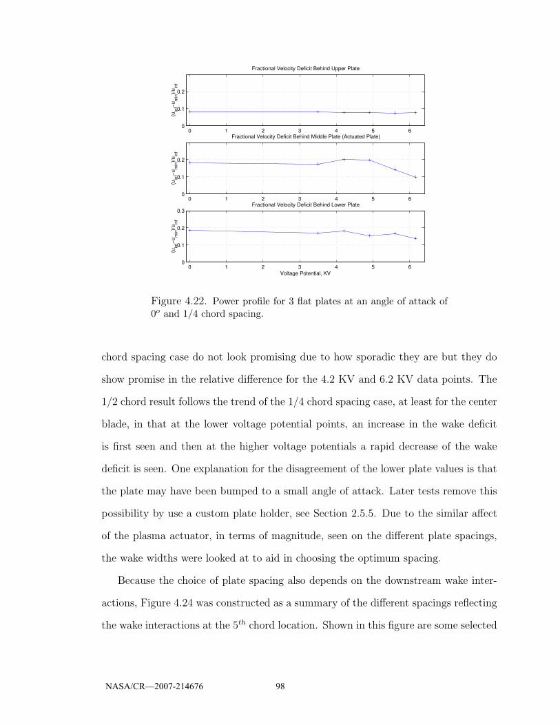
0 1 2 3 4 5 60
0.1
0.2
(uin
f−um
in)/u
inf
Fractional Velocity Deficit Behind Upper Plate
0 1 2 3 4 5 60
0.1
0.2
(uin
f−um
in)/u
inf
Fractional Velocity Deficit Behind Middle Plate (Actuated Plate)
0 1 2 3 4 5 60
0.1
0.2
0.3
Voltage Potential, KV
(uin
f−um
in)/u
inf
Fractional Velocity Deficit Behind Lower Plate
Figure 4.22. Power profile for 3 flat plates at an angle of attack of0o and 1/4 chord spacing.
chord spacing case do not look promising due to how sporadic they are but they do
show promise in the relative difference for the 4.2 KV and 6.2 KV data points. The
1/2 chord result follows the trend of the 1/4 chord spacing case, at least for the center
blade, in that at the lower voltage potential points, an increase in the wake deficit
is first seen and then at the higher voltage potentials a rapid decrease of the wake
deficit is seen. One explanation for the disagreement of the lower plate values is that
the plate may have been bumped to a small angle of attack. Later tests remove this
possibility by use a custom plate holder, see Section 2.5.5. Due to the similar affect
of the plasma actuator, in terms of magnitude, seen on the different plate spacings,
the wake widths were looked at to aid in choosing the optimum spacing.
Because the choice of plate spacing also depends on the downstream wake inter-
actions, Figure 4.24 was constructed as a summary of the different spacings reflecting
the wake interactions at the 5th chord location. Shown in this figure are some selected
NASA/CR—2007-214676 98

0 1 2 3 4 5 60
0.1
0.2
(uin
f−um
in)/u
inf
Fractional Velocity Deficit Behind Upper Plate
0 degree, 1/4 chord spacing0 degree, 3/8 chord spacing0 degree, 1/2 chord spacing
0 1 2 3 4 5 60
0.1
0.2
(uin
f−um
in)/u
inf
Fractional Velocity Deficit Behind Middle Plate (Actuated Plate)
0 1 2 3 4 5 60
0.1
0.2
0.3
Voltage Potential, KV
(uin
f−um
in)/u
inf
Fractional Velocity Deficit Behind Lower Plate
Figure 4.23. Power profile for 3 flat plates at an angle of attack of0o and various plate spacings.
cases of the different voltages for the three different spacings, recall that these were
done at the 5th chord location. The cases chosen were those with the actuator turned
‘off’, 4.2 KV potential, and the maximum voltage potential case of 6.2 KV. The rea-
son for including the 4.2 KV case was that this case had the maximum but opposite
effect of the maximum voltage case. One of the ideas considered here was instead of
working between an ‘off/on’ case, the arrangement would operate between two differ-
ent ‘on’ cases. Thus capitalizing on the maximum relative effect of the actuator and
not relying only on the relative effect compared to the ‘off’ case.
From this data, the 3/8 chord case was chosen to be the case of study. This
was based on the relative difference seen between the minimum and maximum value
shown in Figure 4.23 for the middle plate and the wake interaction shown in Figure
4.24. There was no noticeable wake interaction for the ‘off’ case, and a small amount
in the case with the maximum applied voltage. In terms of the discreetness of the
NASA/CR—2007-214676 99
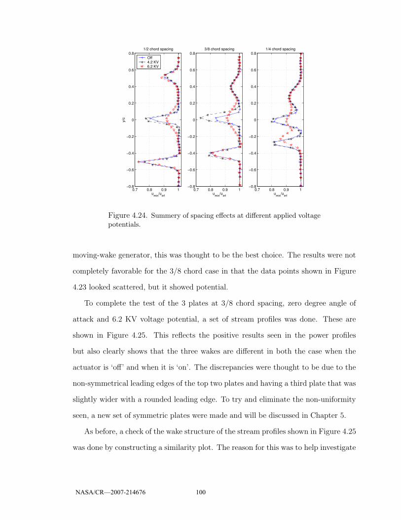
0.7 0.8 0.9 1−0.8
−0.6
−0.4
−0.2
0
0.2
0.4
0.6
0.8
y/c
umin
/uinf
1/2 chord spacing
Off4.2 KV6.2 KV
0.7 0.8 0.9 1−0.8
−0.6
−0.4
−0.2
0
0.2
0.4
0.6
0.8
umin
/uinf
3/8 chord spacing
0.7 0.8 0.9 1−0.8
−0.6
−0.4
−0.2
0
0.2
0.4
0.6
0.8
umin
/uinf
1/4 chord spacing
Figure 4.24. Summery of spacing effects at different applied voltagepotentials.
moving-wake generator, this was thought to be the best choice. The results were not
completely favorable for the 3/8 chord case in that the data points shown in Figure
4.23 looked scattered, but it showed potential.
To complete the test of the 3 plates at 3/8 chord spacing, zero degree angle of
attack and 6.2 KV voltage potential, a set of stream profiles was done. These are
shown in Figure 4.25. This reflects the positive results seen in the power profiles
but also clearly shows that the three wakes are different in both the case when the
actuator is ‘off’ and when it is ‘on’. The discrepancies were thought to be due to the
non-symmetrical leading edges of the top two plates and having a third plate that was
slightly wider with a rounded leading edge. To try and eliminate the non-uniformity
seen, a new set of symmetric plates were made and will be discussed in Chapter 5.
As before, a check of the wake structure of the stream profiles shown in Figure 4.25
was done by constructing a similarity plot. The reason for this was to help investigate
NASA/CR—2007-214676 100
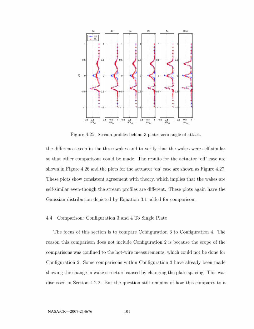
0.6 0.8 1
−1
−0.5
0
0.5
1
u/uinf
0.5c
0.6 0.8 1
−1
−0.5
0
0.5
1
u/uinf
1c
0.6 0.8 1
−1
−0.5
0
0.5
1
u/uinf
2c
0.6 0.8 1
−1
−0.5
0
0.5
1
u/uinf
3c
0.6 0.8 1
−1
−0.5
0
0.5
1
u/uinf
4c
0.6 0.8 1
−1
−0.5
0
0.5
1
u/uinf
y/c
5c
OffOn
Figure 4.25. Stream profiles behind 3 plates zero angle of attack.
the differences seen in the three wakes and to verify that the wakes were self-similar
so that other comparisons could be made. The results for the actuator ‘off’ case are
shown in Figure 4.26 and the plots for the actuator ‘on’ case are shown as Figure 4.27.
These plots show consistent agreement with theory, which implies that the wakes are
self-similar even-though the stream profiles are different. These plots again have the
Gaussian distribution depicted by Equation 3.1 added for comparison.
4.4 Comparison: Configuration 3 and 4 To Single Plate
The focus of this section is to compare Configuration 3 to Configuration 4. The
reason this comparison does not include Configuration 2 is because the scope of the
comparisons was confined to the hot-wire measurements, which could not be done for
Configuration 2. Some comparisons within Configuration 3 have already been made
showing the change in wake structure caused by changing the plate spacing. This was
discussed in Section 4.2.2. But the question still remains of how this compares to a
NASA/CR—2007-214676 101

Figure 4.26. Similarity plot for three flat plates at zero angle ofattack with a 3/8 chord plate spacing and the actuator ‘off’.
Figure 4.27. Similarity plot for three flat plates at zero angle ofattack with a 3/8 chord plate spacing and the actuator ‘on’.
NASA/CR—2007-214676 102
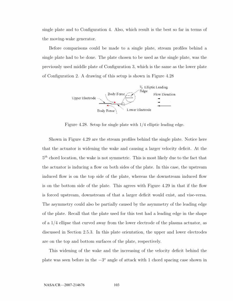
single plate and to Configuration 4. Also, which result is the best so far in terms of
the moving-wake generator.
Before comparisons could be made to a single plate, stream profiles behind a
single plate had to be done. The plate chosen to be used as the single plate, was the
previously used middle plate of Configuration 3, which is the same as the lower plate
of Configuration 2. A drawing of this setup is shown in Figure 4.28
Figure 4.28. Setup for single plate with 1/4 elliptic leading edge.
Shown in Figure 4.29 are the stream profiles behind the single plate. Notice here
that the actuator is widening the wake and causing a larger velocity deficit. At the
5th chord location, the wake is not symmetric. This is most likely due to the fact that
the actuator is inducing a flow on both sides of the plate. In this case, the upstream
induced flow is on the top side of the plate, whereas the downstream induced flow
is on the bottom side of the plate. This agrees with Figure 4.29 in that if the flow
is forced upstream, downstream of that a larger deficit would exist, and vise-versa.
The asymmetry could also be partially caused by the asymmetry of the leading edge
of the plate. Recall that the plate used for this test had a leading edge in the shape
of a 1/4 ellipse that curved away from the lower electrode of the plasma actuator, as
discussed in Section 2.5.3. In this plate orientation, the upper and lower electrodes
are on the top and bottom surfaces of the plate, respectively.
This widening of the wake and the increasing of the velocity deficit behind the
plate was seen before in the −3o angle of attack with 1 chord spacing case shown in
NASA/CR—2007-214676 103

0.6 0.8 1
−1
−0.5
0
0.5
1
u/uinf
0.5c
0.6 0.8 1
−1
−0.5
0
0.5
1
u/uinf
1c
0.6 0.8 1
−1
−0.5
0
0.5
1
u/uinf
2c
0.6 0.8 1
−1
−0.5
0
0.5
1
u/uinf
3c
0.6 0.8 1
−1
−0.5
0
0.5
1
u/uinf
4c
0.6 0.8 1
−1
−0.5
0
0.5
1
u/uinf
y/c
5c
OffOn
Figure 4.29. Stream profiles behind single plate with 1/4 ellipticleading edge.
Figure 4.13. This reinforces the idea that the two plates in the 1 chord spacing case
were acting independently.
Once the stream profiles behind the single plate were done it was important to
compare the relevant results, which would be to the zero angle of attack cases of
Configuration 4. The comparison shown in Figure 4.30, which is a comparison of the
fractional velocity deficits behind each of the plates of the Configuration 4, zero angle
of attack, 3/8 chord plate spacing case shown in Figure 4.25, to the zero angle of
attack, single plate case shown in Figure 4.29. As was done earlier with the different
spacings of Configuration 3, the velocity deficits where expressed as fractions of the
respective local free-stream velocities. In Figure 4.30 there are three subplots. Each
subplot corresponds to one of the three plates in Configuration 4 and shows the deficits
for that plate. The unactuated (top and bottom) plates are included to show any
affect that the actuator may cause on the neighboring plates. The top subplot shows
NASA/CR—2007-214676 104
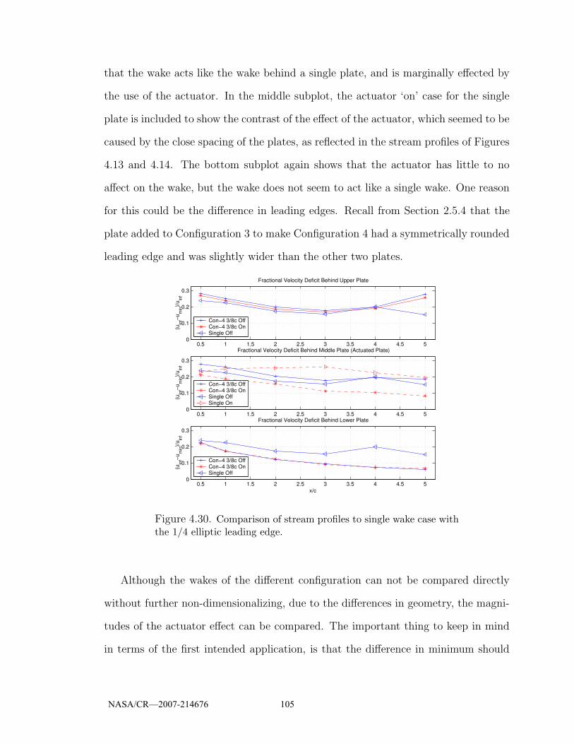
that the wake acts like the wake behind a single plate, and is marginally effected by
the use of the actuator. In the middle subplot, the actuator ‘on’ case for the single
plate is included to show the contrast of the effect of the actuator, which seemed to be
caused by the close spacing of the plates, as reflected in the stream profiles of Figures
4.13 and 4.14. The bottom subplot again shows that the actuator has little to no
affect on the wake, but the wake does not seem to act like a single wake. One reason
for this could be the difference in leading edges. Recall from Section 2.5.4 that the
plate added to Configuration 3 to make Configuration 4 had a symmetrically rounded
leading edge and was slightly wider than the other two plates.
0.5 1 1.5 2 2.5 3 3.5 4 4.5 50
0.1
0.2
0.3
(uin
f−um
in)/u
inf
Fractional Velocity Deficit Behind Upper Plate
Con−4 3/8c OffCon−4 3/8c OnSingle Off
0.5 1 1.5 2 2.5 3 3.5 4 4.5 50
0.1
0.2
0.3
(uin
f−um
in)/u
inf
Fractional Velocity Deficit Behind Middle Plate (Actuated Plate)
Con−4 3/8c OffCon−4 3/8c OnSingle OffSingle On
0.5 1 1.5 2 2.5 3 3.5 4 4.5 50
0.1
0.2
0.3
x/c
(uin
f−um
in)/u
inf
Fractional Velocity Deficit Behind Lower Plate
Con−4 3/8c OffCon−4 3/8c OnSingle Off
Figure 4.30. Comparison of stream profiles to single wake case withthe 1/4 elliptic leading edge.
Although the wakes of the different configuration can not be compared directly
without further non-dimensionalizing, due to the differences in geometry, the magni-
tudes of the actuator effect can be compared. The important thing to keep in mind
in terms of the first intended application, is that the difference in minimum should
NASA/CR—2007-214676 105
be the greatest at the 5th chord location. This way, pulsing the actuator ‘on’ and
‘off’ would cause a large velocity fluctuation whose frequency can be controlled by
the frequency of the pulsing.
To summarize the results thus far, and better illustrate the actuator effect at the
5th chord location, Figure 4.31 was constructed to compare the magnitudes of the
actuator effect at the 5th chord location. This figure shows the value of the difference
of the velocity deficit between the ‘off’ and ‘on’ cases for the wake profiles. Below the
figure is a table that has a description that corresponds to the number designation in
the figure. This figure contains a large amount of information in that it summarizes
all of the stream profile cases and all of the power profile cases done thus far using
the plasma actuator.
Many conclusions can be drawn from Figure 4.31. For instance, the −3o angle of
attack, 1/2 chord spacing, cases of Configuration 3 are clearly the best in terms of
the magnitude. However, keep in mind that the voltage supplied to the actuator for
these cases was 11.2 KV. This voltage potential has the drawback of reducing the life
of the actuator.
Also, the addition of the third plate making Configuration 4 may have hindered
effect of the actuator but the degree of this is unknown because the voltage potential
and was also changed between the two configurations. This effect is seen by comparing
Designations 3 and 6. In the comparison of Designations 6 and 7, the reduced spacing
hurt the performance of the actuator.
Comparisons of Designations 8, 10, and 11, also show the benefit of the wider
spacing. However, based on the results of designations 2 and 3, this improvement is
only beneficial to a point.
Lastly, comparing the results for Designations 9 and 10 shows some inconsistency
in the result in that these two experimental setups were the same; the only difference
NASA/CR—2007-214676 106

was how the data was gathered. The values in Designation 9 were obtained from a
power profile, and the values for Designation 10 were from the velocity stream profile.
Over all, the results thus far have been favorable. The −3o angle of attack, 1/2
chord spacing, cases of Configuration 3 have the best results but require more power,
limiting the actuator life span, and have the potential to be more intrusive to the
flow. The zero degree angle of attack cases of Configuration 4 show the most promise
in terms of the effect for the power required and the intrusiveness on the flow. Based
on the wake comparisons of Configuration 4 for the different spacings, the 3/8 chord
case seemed to be the best and was chosen for the next set of experiments using
uniformly produced flat plates. This is discussed in Chapter 5.
NASA/CR—2007-214676 107
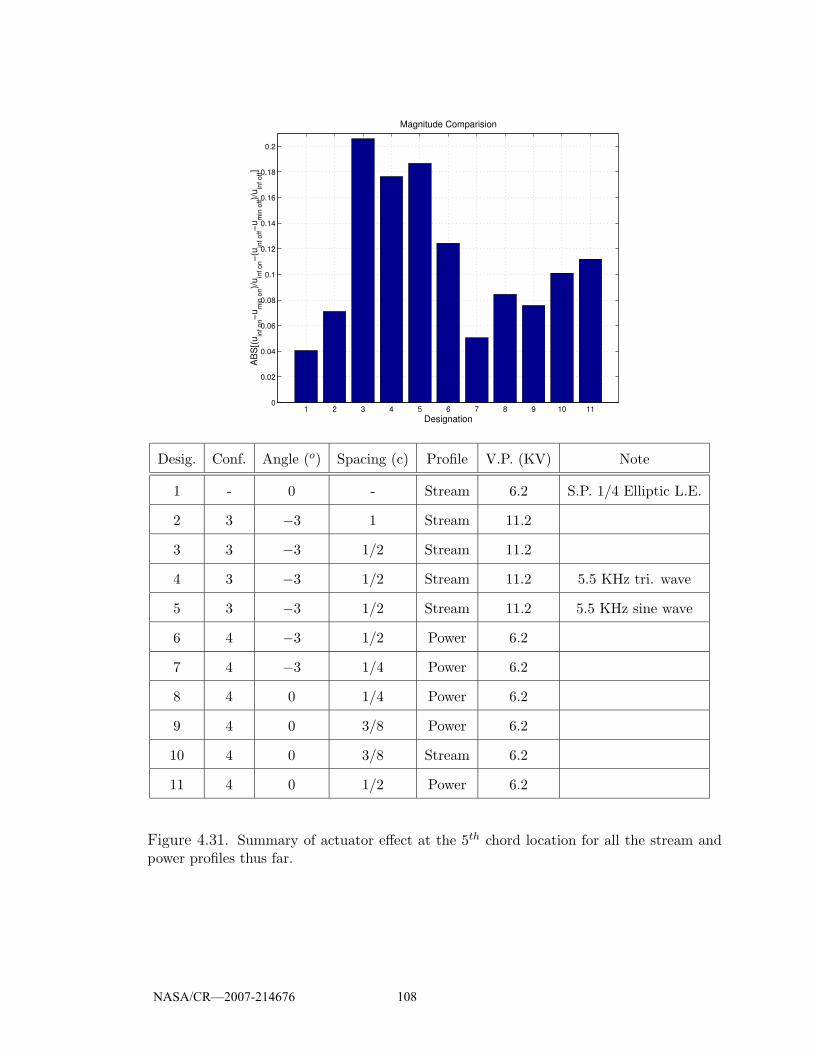
1 2 3 4 5 6 7 8 9 10 110
0.02
0.04
0.06
0.08
0.1
0.12
0.14
0.16
0.18
0.2
AB
S[(u
inf o
n−um
in o
n)/uin
f on−(
u inf o
ff−um
in o
ff)/uin
f off]
Designation
Magnitude Comparision
Desig. Conf. Angle (o) Spacing (c) Profile V.P. (KV) Note
1 - 0 - Stream 6.2 S.P. 1/4 Elliptic L.E.
2 3 −3 1 Stream 11.2
3 3 −3 1/2 Stream 11.2
4 3 −3 1/2 Stream 11.2 5.5 KHz tri. wave
5 3 −3 1/2 Stream 11.2 5.5 KHz sine wave
6 4 −3 1/2 Power 6.2
7 4 −3 1/4 Power 6.2
8 4 0 1/4 Power 6.2
9 4 0 3/8 Power 6.2
10 4 0 3/8 Stream 6.2
11 4 0 1/2 Power 6.2
Figure 4.31. Summary of actuator effect at the 5th chord location for all the stream andpower profiles thus far.
NASA/CR—2007-214676 108
CHAPTER 5
RESULTS: UNIFORM FLAT PLATES
After compiling the previous results and observing the sensitivity of the plates
due to spacing and orientation, it was decided to repeat the experiments. This time
however, using plates that were fabricated as uniform as possible. This was referred
to earlier as Configuration 5. The intent with the new setup was to try to eliminate
one of the variables contributing to the inconsistencies observed in the experimental
results. As such, the plates were re-manufactured on a LPKF CNC milling machine
designed for the manufacturing of prototype circuit boards. In addition to these
plates, a new type of plate/actuator setup was made using the LPKF CNC machine
and was referred to as Configuration 6 in Section 2.5.6. Configurations 5 and 6 will
both be discussed in this chapter.
5.1 Configuration 5
The first investigation made using the new plates, was to check the uniformity of
the wakes behind the plates. As the first experiment, each plate was assigned a letter,
A,B, or C and wake profiles were done behind the plates at the 5th downstream chord
location. All six permutations of the letters A, B, and C, meaning the plate orders,
were tested. The results of this are shown in Figure 5.1. If the setup was perfect and
all of the plates were identical regardless of the plate order, the wake profiles would
all be the same. It is apparent from this figure that some imperfections must still
NASA/CR—2007-214676 109
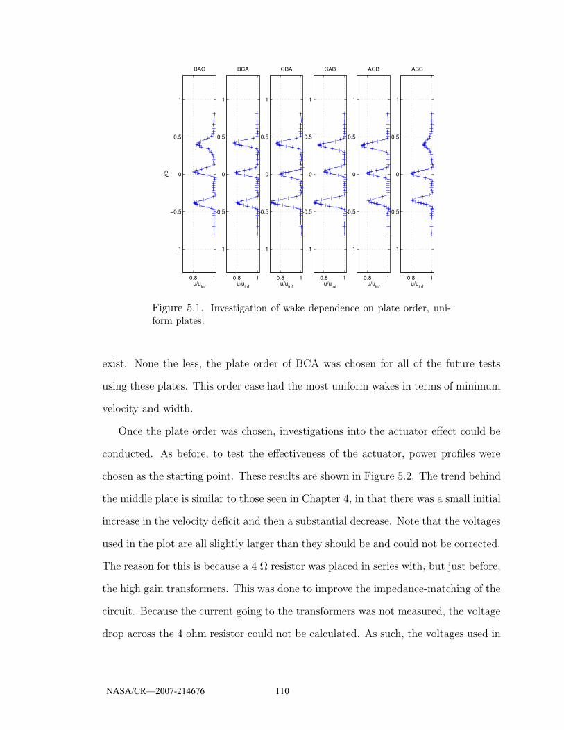
0.8 1
−1
−0.5
0
0.5
1
u/uinf
ABC
0.8 1
−1
−0.5
0
0.5
1
u/uinf
ACB
0.8 1
−1
−0.5
0
0.5
1
u/uinf
CAB
0.8 1
−1
−0.5
0
0.5
1
u/uinf
CBA
0.8 1
−1
−0.5
0
0.5
1
u/uinf
BCA
0.8 1
−1
−0.5
0
0.5
1
u/uinf
y/c
BAC
Figure 5.1. Investigation of wake dependence on plate order, uni-form plates.
exist. None the less, the plate order of BCA was chosen for all of the future tests
using these plates. This order case had the most uniform wakes in terms of minimum
velocity and width.
Once the plate order was chosen, investigations into the actuator effect could be
conducted. As before, to test the effectiveness of the actuator, power profiles were
chosen as the starting point. These results are shown in Figure 5.2. The trend behind
the middle plate is similar to those seen in Chapter 4, in that there was a small initial
increase in the velocity deficit and then a substantial decrease. Note that the voltages
used in the plot are all slightly larger than they should be and could not be corrected.
The reason for this is because a 4 Ω resistor was placed in series with, but just before,
the high gain transformers. This was done to improve the impedance-matching of the
circuit. Because the current going to the transformers was not measured, the voltage
drop across the 4 ohm resistor could not be calculated. As such, the voltages used in
NASA/CR—2007-214676 110

0 1 2 3 4 5 60
0.1
0.2
(uin
f−um
in)/u
inf
Fractional Velocity Deficit Behind Upper Plate
0 1 2 3 4 5 60
0.1
0.2(u
inf−u
min
)/uin
f
Fractional Velocity Deficit Behind Middle Plate (Actuated Plate)
0 1 2 3 4 5 60
0.1
0.2
0.3
Voltage Potential, KV
(uin
f−um
in)/u
inf
Fractional Velocity Deficit Behind Lower Plate
Figure 5.2. Power profiles for 3 uniform plates at zero angle of attackwith 3/8 chord spacing.
the plot are the theoretical values without the resistor.
The addition of the resistor did enable the plasma system to obtain higher voltage
potentials, as measured before the resistor. The degree to which this improved the
system, in terms of the voltage potential at the actuator, was not determined.
After looking at some of the previous data it was decided to repeat the power
profiles shown in Figure 5.2, but this time increasing the maximum voltage potential
across the actuator to 7.7 KV. This was the new maximum voltage of the system with
the 4 Ω resistor. This test was done to check earlier results that indicated a peak effect
at a voltage potential lower than what the plasma system was capable of supplying.
Also this second test was done to see if the previous chosen optimum voltage of
6.3 KV changed at all from the addition of the 4 Ω resistor. If the magnitudes of
the velocity deficits shifted to a higher voltage value, meaning that actual velocity
deficits decreased at the different voltage potentials, it would imply that the added 4
NASA/CR—2007-214676 111
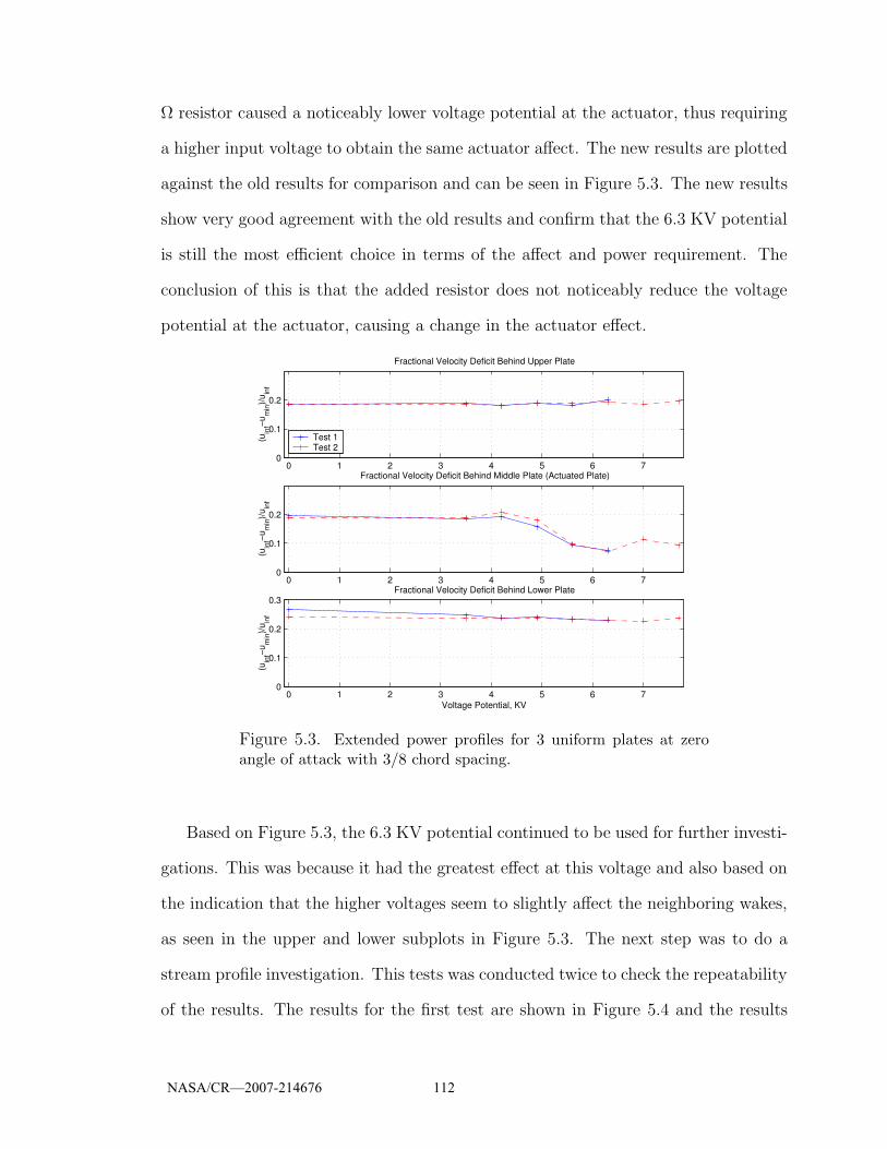
Ω resistor caused a noticeably lower voltage potential at the actuator, thus requiring
a higher input voltage to obtain the same actuator affect. The new results are plotted
against the old results for comparison and can be seen in Figure 5.3. The new results
show very good agreement with the old results and confirm that the 6.3 KV potential
is still the most efficient choice in terms of the affect and power requirement. The
conclusion of this is that the added resistor does not noticeably reduce the voltage
potential at the actuator, causing a change in the actuator effect.
0 1 2 3 4 5 6 70
0.1
0.2
(uin
f−um
in)/u
inf
Fractional Velocity Deficit Behind Upper Plate
Test 1Test 2
0 1 2 3 4 5 6 70
0.1
0.2
(uin
f−um
in)/u
inf
Fractional Velocity Deficit Behind Middle Plate (Actuated Plate)
0 1 2 3 4 5 6 70
0.1
0.2
0.3
Voltage Potential, KV
(uin
f−um
in)/u
inf
Fractional Velocity Deficit Behind Lower Plate
Figure 5.3. Extended power profiles for 3 uniform plates at zeroangle of attack with 3/8 chord spacing.
Based on Figure 5.3, the 6.3 KV potential continued to be used for further investi-
gations. This was because it had the greatest effect at this voltage and also based on
the indication that the higher voltages seem to slightly affect the neighboring wakes,
as seen in the upper and lower subplots in Figure 5.3. The next step was to do a
stream profile investigation. This tests was conducted twice to check the repeatability
of the results. The results for the first test are shown in Figure 5.4 and the results
NASA/CR—2007-214676 112

for the second test are shown in Figure 5.5.
0.6 0.8 1
−1
−0.5
0
0.5
1
u/uinf
0.5c
0.6 0.8 1
−1
−0.5
0
0.5
1
u/uinf
1c
0.6 0.8 1
−1
−0.5
0
0.5
1
u/uinf
2c
0.6 0.8 1
−1
−0.5
0
0.5
1
u/uinf
3c
0.6 0.8 1
−1
−0.5
0
0.5
1
u/uinf
4c
0.6 0.8 1
−1
−0.5
0
0.5
1
u/uinf
y/c
5c
OffOn
Figure 5.4. Stream profiles for first test of uniform plates.
0.6 0.8 1
−1
−0.5
0
0.5
1
u/uinf
0.5c
0.6 0.8 1
−1
−0.5
0
0.5
1
u/uinf
1c
0.6 0.8 1
−1
−0.5
0
0.5
1
u/uinf
2c
0.6 0.8 1
−1
−0.5
0
0.5
1
u/uinf
3c
0.6 0.8 1
−1
−0.5
0
0.5
1
u/uinf
4c
0.6 0.8 1
−1
−0.5
0
0.5
1
u/uinf
y/c
5c
OffOn
Figure 5.5. Stream profiles for second test of uniform plates.
NASA/CR—2007-214676 113

To ease the comparison, the fractional velocity deficits of the wakes were replotted
together in Figure 5.6. The results from the second experiment were slightly better
than the first set in that at the 5th chord location, the second test shows approximately
2 percent more of a velocity deficit. The deficits behind the other plates for both the
‘off’ and ‘on’ cases agreed well. Overall, the trends were similar to the ‘off/on’ cases
shown previously and the results were deemed to be sufficient to try another setup,
after comparing to a single plate.
0.5 1 1.5 2 2.5 3 3.5 4 4.5 50
0.1
0.2
0.3
(uin
f−um
in)/u
inf
Fractional Velocity Deficit Behind Upper Plate
Test 1 OffTest 1 OnTest 2 OffTest 2 On
0.5 1 1.5 2 2.5 3 3.5 4 4.5 50
0.1
0.2
0.3
(uin
f−um
in)/u
inf
Fractional Velocity Deficit Behind Middle Plate (Actuated Plate)
0.5 1 1.5 2 2.5 3 3.5 4 4.5 50
0.1
0.2
0.3
x/c
(uin
f−um
in)/u
inf
Fractional Velocity Deficit Behind Lower Plate
Figure 5.6. Wake decay comparison for the two sets of stream pro-files.
5.1.1 Comparison: Configuration 5 To Single Plate
As with the last chapter, it was desired to compare the aforementioned results of
Configuration 5 to a single plate. However, because the leading edges of the uniform
plates were different than what was used in the previous experiments, the single plate
tests had to be repeated, using one of the new uniform plates, before the comparison
NASA/CR—2007-214676 114
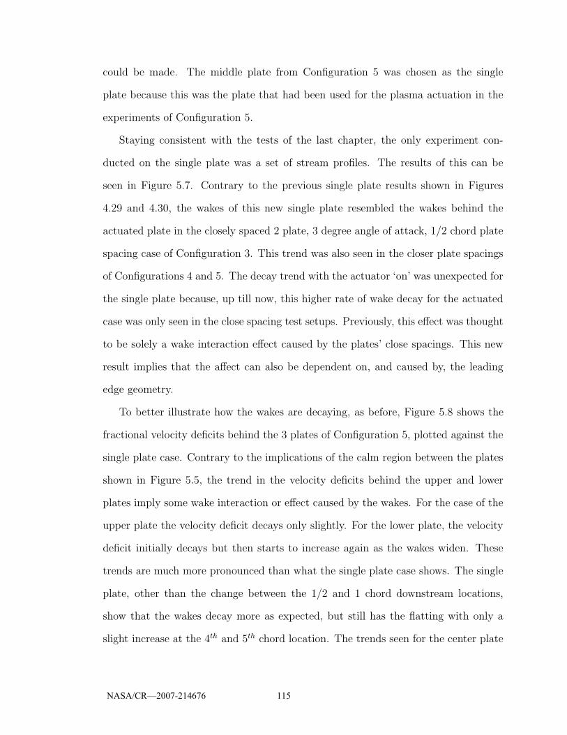
could be made. The middle plate from Configuration 5 was chosen as the single
plate because this was the plate that had been used for the plasma actuation in the
experiments of Configuration 5.
Staying consistent with the tests of the last chapter, the only experiment con-
ducted on the single plate was a set of stream profiles. The results of this can be
seen in Figure 5.7. Contrary to the previous single plate results shown in Figures
4.29 and 4.30, the wakes of this new single plate resembled the wakes behind the
actuated plate in the closely spaced 2 plate, 3 degree angle of attack, 1/2 chord plate
spacing case of Configuration 3. This trend was also seen in the closer plate spacings
of Configurations 4 and 5. The decay trend with the actuator ‘on’ was unexpected for
the single plate because, up till now, this higher rate of wake decay for the actuated
case was only seen in the close spacing test setups. Previously, this effect was thought
to be solely a wake interaction effect caused by the plates’ close spacings. This new
result implies that the affect can also be dependent on, and caused by, the leading
edge geometry.
To better illustrate how the wakes are decaying, as before, Figure 5.8 shows the
fractional velocity deficits behind the 3 plates of Configuration 5, plotted against the
single plate case. Contrary to the implications of the calm region between the plates
shown in Figure 5.5, the trend in the velocity deficits behind the upper and lower
plates imply some wake interaction or effect caused by the wakes. For the case of the
upper plate the velocity deficit decays only slightly. For the lower plate, the velocity
deficit initially decays but then starts to increase again as the wakes widen. These
trends are much more pronounced than what the single plate case shows. The single
plate, other than the change between the 1/2 and 1 chord downstream locations,
show that the wakes decay more as expected, but still has the flatting with only a
slight increase at the 4th and 5th chord location. The trends seen for the center plate
NASA/CR—2007-214676 115
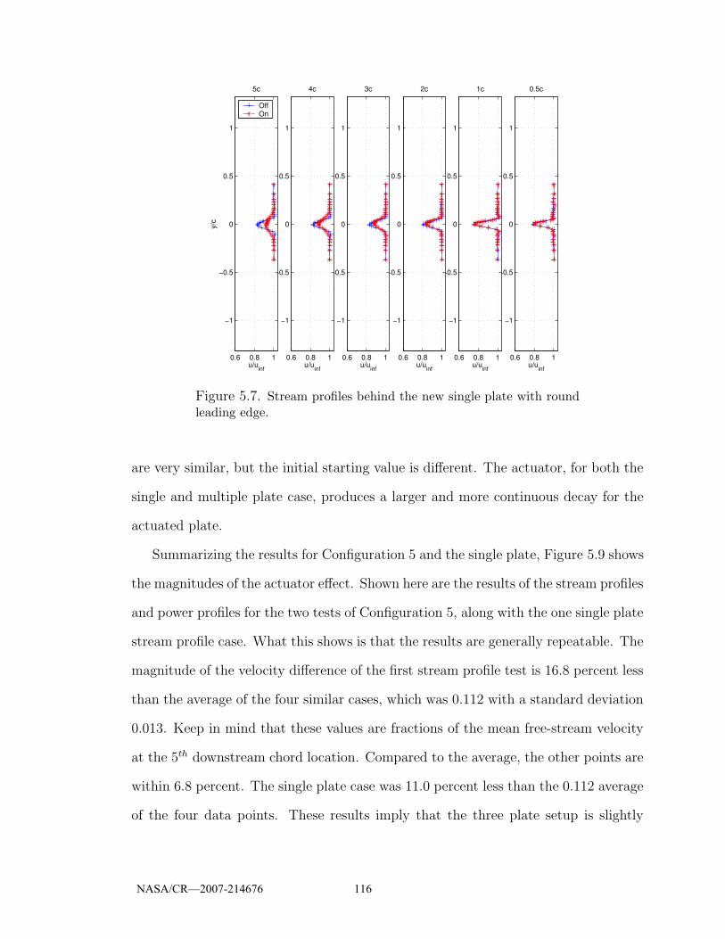
0.6 0.8 1
−1
−0.5
0
0.5
1
u/uinf
0.5c
0.6 0.8 1
−1
−0.5
0
0.5
1
u/uinf
1c
0.6 0.8 1
−1
−0.5
0
0.5
1
u/uinf
2c
0.6 0.8 1
−1
−0.5
0
0.5
1
u/uinf
3c
0.6 0.8 1
−1
−0.5
0
0.5
1
u/uinf
4c
0.6 0.8 1
−1
−0.5
0
0.5
1
u/uinf
y/c
5c
OffOn
Figure 5.7. Stream profiles behind the new single plate with roundleading edge.
are very similar, but the initial starting value is different. The actuator, for both the
single and multiple plate case, produces a larger and more continuous decay for the
actuated plate.
Summarizing the results for Configuration 5 and the single plate, Figure 5.9 shows
the magnitudes of the actuator effect. Shown here are the results of the stream profiles
and power profiles for the two tests of Configuration 5, along with the one single plate
stream profile case. What this shows is that the results are generally repeatable. The
magnitude of the velocity difference of the first stream profile test is 16.8 percent less
than the average of the four similar cases, which was 0.112 with a standard deviation
0.013. Keep in mind that these values are fractions of the mean free-stream velocity
at the 5th downstream chord location. Compared to the average, the other points are
within 6.8 percent. The single plate case was 11.0 percent less than the 0.112 average
of the four data points. These results imply that the three plate setup is slightly
NASA/CR—2007-214676 116
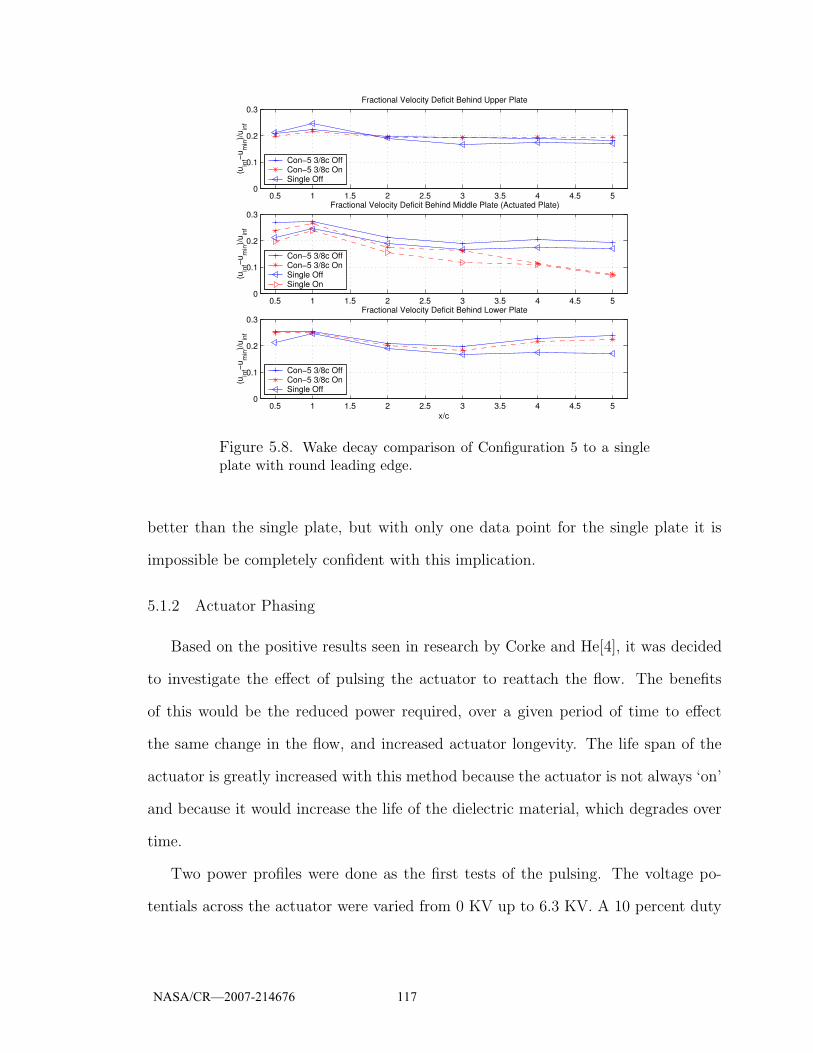
0.5 1 1.5 2 2.5 3 3.5 4 4.5 50
0.1
0.2
0.3
(uin
f−um
in)/u
inf
Fractional Velocity Deficit Behind Upper Plate
Con−5 3/8c OffCon−5 3/8c OnSingle Off
0.5 1 1.5 2 2.5 3 3.5 4 4.5 50
0.1
0.2
0.3
(uin
f−um
in)/u
inf
Fractional Velocity Deficit Behind Middle Plate (Actuated Plate)
Con−5 3/8c OffCon−5 3/8c OnSingle OffSingle On
0.5 1 1.5 2 2.5 3 3.5 4 4.5 50
0.1
0.2
0.3
x/c
(uin
f−um
in)/u
inf
Fractional Velocity Deficit Behind Lower Plate
Con−5 3/8c OffCon−5 3/8c OnSingle Off
Figure 5.8. Wake decay comparison of Configuration 5 to a singleplate with round leading edge.
better than the single plate, but with only one data point for the single plate it is
impossible be completely confident with this implication.
5.1.2 Actuator Phasing
Based on the positive results seen in research by Corke and He[4], it was decided
to investigate the effect of pulsing the actuator to reattach the flow. The benefits
of this would be the reduced power required, over a given period of time to effect
the same change in the flow, and increased actuator longevity. The life span of the
actuator is greatly increased with this method because the actuator is not always ‘on’
and because it would increase the life of the dielectric material, which degrades over
time.
Two power profiles were done as the first tests of the pulsing. The voltage po-
tentials across the actuator were varied from 0 KV up to 6.3 KV. A 10 percent duty
NASA/CR—2007-214676 117
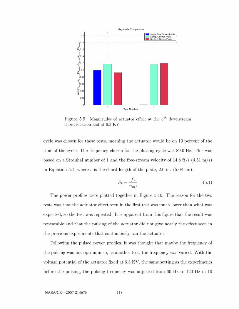
1 20
0.02
0.04
0.06
0.08
0.1
0.12
0.14
0.16
0.18
0.2
AB
S[(u
inf o
n−um
in o
n)/uin
f on−(
u inf o
ff−um
in o
ff)/uin
f off]
Test Number
Magnitude Comparision
Single Plate Stream ProfileConfig. 5 Power ProfileConfig. 5 Stream Profile
Figure 5.9. Magnitudes of actuator effect at the 5th downstreamchord location and at 6.3 KV.
cycle was chosen for these tests, meaning the actuator would be on 10 percent of the
time of the cycle. The frequency chosen for the phasing cycle was 89.0 Hz. This was
based on a Strouhal number of 1 and the free-stream velocity of 14.8 ft/s (4.51 m/s)
in Equation 5.1, where c is the chord length of the plate, 2.0 in. (5.08 cm).
St =fc
uinf(5.1)
The power profiles were plotted together in Figure 5.10. The reason for the two
tests was that the actuator effect seen in the first test was much lower than what was
expected, so the test was repeated. It is apparent from this figure that the result was
repeatable and that the pulsing of the actuator did not give nearly the effect seen in
the previous experiments that continuously ran the actuator.
Following the pulsed power profiles, it was thought that maybe the frequency of
the pulsing was not optimum so, as another test, the frequency was varied. With the
voltage potential of the actuator fixed at 6.3 KV, the same setting as the experiments
before the pulsing, the pulsing frequency was adjusted from 60 Hz to 120 Hz in 10
NASA/CR—2007-214676 118

0 1 2 3 4 5 60
0.1
0.2
(uin
f−um
in)/u
inf
Fractional Velocity Deficit Behind Upper Plate
Test 1Test 2
0 1 2 3 4 5 60
0.1
0.2(u
inf−u
min
)/uin
f
Fractional Velocity Deficit Behind Middle Plate (Actuated Plate)
0 1 2 3 4 5 60
0.1
0.2
0.3
Voltage Potential, KV
(uin
f−um
in)/u
inf
Fractional Velocity Deficit Behind Lower Plate
Figure 5.10. Effect of pulsing the plasma actuator at 89.0 Hz witha 10 percent duty cycle. Plates are at zero angle of attack with 3/8chord spacing.
Hz increments. Note that the zero frequency case in the plot was a base profile done
with the actuator ‘off’. These tests were again done twice and the results of this
can be seen in Figure 5.11. In this plot, the Strouhal number was calculated based
on the average free-stream value for each run. From this, it was apparent that the
pulsing had little effect. Arguably, the 10 Hz step size was too large to pinpoint the
best frequency but from the results, it was thought that even at the “best” frequency
the actuator effect for this setup was not going to be as good as previously seen.
Therefore, this area of testing was discontinued and tests on Configuration 6 were
started. Due to how little affect the actuator had, the results of the phasing will not
compared to other data.
NASA/CR—2007-214676 119

0 0.2 0.4 0.6 0.8 1 1.2 1.40
0.1
0.2
0.3
(uin
f−um
in)/u
inf
Fractional Velocity Deficit Behind Upper Plate
Test 1Test 2
0 0.2 0.4 0.6 0.8 1 1.2 1.40
0.1
0.2
0.3
(uin
f−um
in)/u
inf
Fractional Velocity Deficit Behind Middle Plate (Actuated Plate)
0 0.2 0.4 0.6 0.8 1 1.2 1.40
0.1
0.2
0.3
Strouhal Number, St
(uin
f−um
in)/u
inf
Fractional Velocity Deficit Behind Lower Plate
Figure 5.11. Effect of pulsing the plasma actuator over frequencyrange from 60 Hz to 120 Hz, at a 6.3 KV voltage potential.
5.2 Configuration 6
Though many of the results thus far were good, it was still thought improvements
could be made. To this end, one more configuration was tested, Configuration 6,
which was the sandwiched electrode configuration. The basic concept here was that
two actuators should be better than one. Recall that this setup has an upper electrode
on either side of the plate such that the flow induced by the actuators is forcing the
free-stream flow in the same direction on both sides of the plate. Up till now, the
actuator forced the flow upstream on one side of the plate and downstream on the
other side. Both plate orientations of Configuration 6 were tried, That is, forcing the
flow upstream and forcing the flow downstream. The results will be presented in the
following two sections.
NASA/CR—2007-214676 120
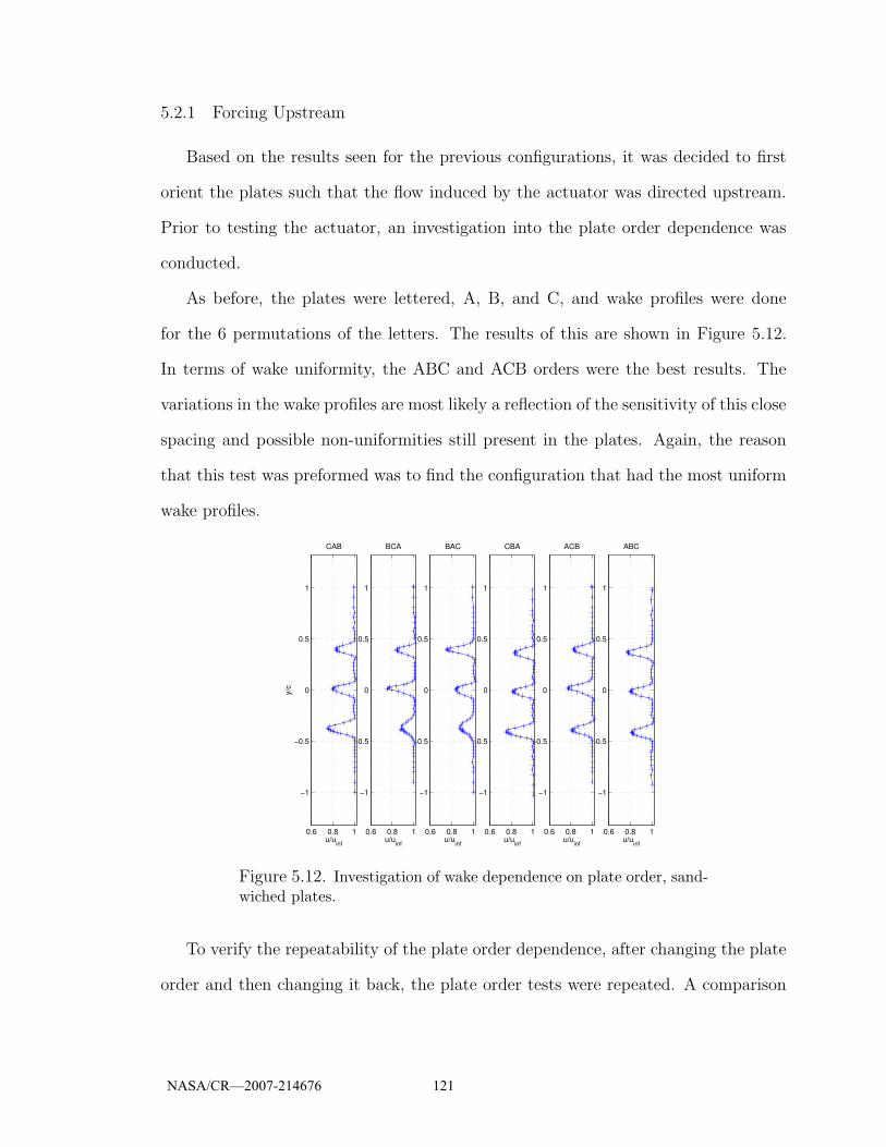
5.2.1 Forcing Upstream
Based on the results seen for the previous configurations, it was decided to first
orient the plates such that the flow induced by the actuator was directed upstream.
Prior to testing the actuator, an investigation into the plate order dependence was
conducted.
As before, the plates were lettered, A, B, and C, and wake profiles were done
for the 6 permutations of the letters. The results of this are shown in Figure 5.12.
In terms of wake uniformity, the ABC and ACB orders were the best results. The
variations in the wake profiles are most likely a reflection of the sensitivity of this close
spacing and possible non-uniformities still present in the plates. Again, the reason
that this test was preformed was to find the configuration that had the most uniform
wake profiles.
0.6 0.8 1
−1
−0.5
0
0.5
1
u/uinf
ABC
0.6 0.8 1
−1
−0.5
0
0.5
1
u/uinf
ACB
0.6 0.8 1
−1
−0.5
0
0.5
1
u/uinf
CBA
0.6 0.8 1
−1
−0.5
0
0.5
1
u/uinf
BAC
0.6 0.8 1
−1
−0.5
0
0.5
1
u/uinf
BCA
0.6 0.8 1
−1
−0.5
0
0.5
1
u/uinf
y/c
CAB
Figure 5.12. Investigation of wake dependence on plate order, sand-wiched plates.
To verify the repeatability of the plate order dependence, after changing the plate
order and then changing it back, the plate order tests were repeated. A comparison
NASA/CR—2007-214676 121
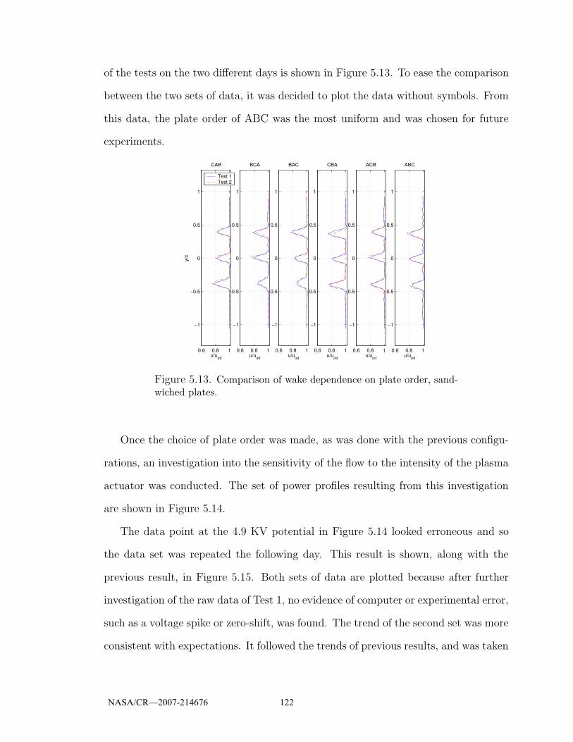
of the tests on the two different days is shown in Figure 5.13. To ease the comparison
between the two sets of data, it was decided to plot the data without symbols. From
this data, the plate order of ABC was the most uniform and was chosen for future
experiments.
0.6 0.8 1
−1
−0.5
0
0.5
1
u/uinf
ABC
0.6 0.8 1
−1
−0.5
0
0.5
1
u/uinf
ACB
0.6 0.8 1
−1
−0.5
0
0.5
1
u/uinf
CBA
0.6 0.8 1
−1
−0.5
0
0.5
1
u/uinf
BAC
0.6 0.8 1
−1
−0.5
0
0.5
1
u/uinf
BCA
0.6 0.8 1
−1
−0.5
0
0.5
1
u/uinf
y/c
CAB
Test 1Test 2
Figure 5.13. Comparison of wake dependence on plate order, sand-wiched plates.
Once the choice of plate order was made, as was done with the previous configu-
rations, an investigation into the sensitivity of the flow to the intensity of the plasma
actuator was conducted. The set of power profiles resulting from this investigation
are shown in Figure 5.14.
The data point at the 4.9 KV potential in Figure 5.14 looked erroneous and so
the data set was repeated the following day. This result is shown, along with the
previous result, in Figure 5.15. Both sets of data are plotted because after further
investigation of the raw data of Test 1, no evidence of computer or experimental error,
such as a voltage spike or zero-shift, was found. The trend of the second set was more
consistent with expectations. It followed the trends of previous results, and was taken
NASA/CR—2007-214676 122

0 1 2 3 4 5 60
0.1
0.2
(uin
f−um
in)/u
inf
Fractional Velocity Deficit Behind Upper Plate
0 1 2 3 4 5 60
0.1
0.2
(uin
f−um
in)/u
inf
Fractional Velocity Deficit Behind Middle Plate (Actuated Plate)
0 1 2 3 4 5 60
0.1
0.2
0.3
Voltage Potential, KV
(uin
f−um
in)/u
inf
Fractional Velocity Deficit Behind Lower Plate
Figure 5.14. Power profile for Configuration 6 forcing upstream.
to be acceptable enough to continue on with other experiments.
The results in Figure 5.15 show that the actuator had the largest effect at the
6.3 KV potential. The next step was to obtain a complete set of stream profiles.
These results are shown in Figure 5.16. The actuator effect appears to be similar to
previous results in that the actuator seemed to work to increase the rate of decay of
the velocity deficit. Notice though that at the 3rd chord position the opposite effect
occurred. Comparisons will be made in Chapter 6 to see if this setup is better or
worse than Configuration 5 at the 5th chord location.
As done with the previous results, Figure 5.17 shows the velocity decay of the
wakes. From this figure it can be seen that after around the 3rd chord position,
with the exception of the middle plate’s wake with the actuator on, the wake deficits
start to grow after the initial decay. The middle subplot, showing the case with the
actuator on, shows a jump in the velocity towards the free-stream value. The wakes
are expected to uniformly decay with downstream location. The opposite effect is
seen after the 3rd chord position and again is most likely due to the wake interactions,
NASA/CR—2007-214676 123

0 1 2 3 4 5 60
0.1
0.2
(uin
f−um
in)/u
inf
Fractional Velocity Deficit Behind Upper Plate
Test 1Test 2
0 1 2 3 4 5 60
0.1
0.2
(uin
f−um
in)/u
inf
Fractional Velocity Deficit Behind Middle Plate (Actuated Plate)
0 1 2 3 4 5 60
0.1
0.2
0.3
Voltage Potential, KV
(uin
f−um
in)/u
inf
Fractional Velocity Deficit Behind Lower Plate
Figure 5.15. Power profile comparison for Configuration 6 forcingupstream.
0.6 0.8 1
−1
−0.5
0
0.5
1
u/uinf
0.5c
0.6 0.8 1
−1
−0.5
0
0.5
1
u/uinf
1c
0.6 0.8 1
−1
−0.5
0
0.5
1
u/uinf
2c
0.6 0.8 1
−1
−0.5
0
0.5
1
u/uinf
3c
0.6 0.8 1
−1
−0.5
0
0.5
1
u/uinf
4c
0.6 0.8 1
−1
−0.5
0
0.5
1
u/uinf
y/c
5c
OffOn
Figure 5.16. Stream profiles for Configuration 6, forcing upstream.
NASA/CR—2007-214676 124

which can occur more downstream as the wakes widen. This plot also shows that the
actuator has little effect on the wakes of the neighboring plates. In addition to the
minimum velocities, some theoretical trend lines were included to help illustrate how
the decay rates start to deviate from theory further downstream. The theoretical
trends again follow Equation 3.2.
0.5 1 1.5 2 2.5 3 3.5 4 4.5 50
0.1
0.2
(uin
f−um
in)/u
inf
Fractional Velocity Deficit Behind Upper Plate
OffOn1/(10.5sqrt(x))+.137
0.5 1 1.5 2 2.5 3 3.5 4 4.5 50
0.1
0.2
(uin
f−um
in)/u
inf
Fractional Velocity Deficit Behind Middle Plate (Actuated Plate)
OffOn1/(10.5sqrt(x))+.155
0.5 1 1.5 2 2.5 3 3.5 4 4.5 50
0.1
0.2
0.3
x/c
(uin
f−um
in)/u
inf
Fractional Velocity Deficit Behind Lower Plate
OffOn1/(10.5sqrt(x))+.132
Figure 5.17. Wake decay for Configuration 6, forcing upstream.
Because of the jump seen in the data points of the actuated plate in Figure 5.17,
the tests were repeated. The second test results were plotted against the first and
are shown in Figure 5.18. Up to the 3rd chord position, the new results show good
agreement with previous tests, but after the 3rd chord position the actuator seems to
have little effect. It is apparent that the base case, that is with the actuator off, does
not agree after the 3rd chord position. The reason(s) for this disagreement is unclear
at this point. Even though the cases with the actuator ‘off’ do not agree for the two
tests, the actuator effect for the two tests does not agree in a manner consistent with
the disagreement of the base cases. In other words, the actuator effect for the second
NASA/CR—2007-214676 125
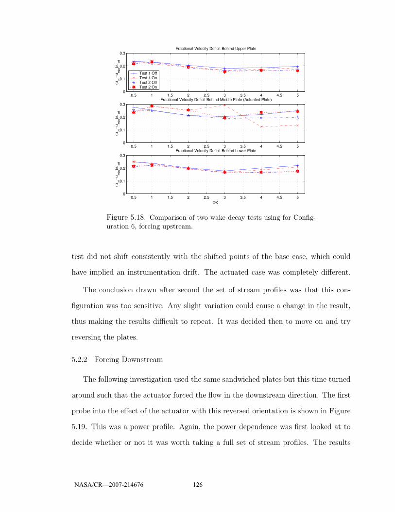
0.5 1 1.5 2 2.5 3 3.5 4 4.5 50
0.1
0.2
0.3
(uin
f−um
in)/u
inf
Fractional Velocity Deficit Behind Upper Plate
Test 1 OffTest 1 OnTest 2 OffTest 2 On
0.5 1 1.5 2 2.5 3 3.5 4 4.5 50
0.1
0.2
0.3
(uin
f−um
in)/u
inf
Fractional Velocity Deficit Behind Middle Plate (Actuated Plate)
0.5 1 1.5 2 2.5 3 3.5 4 4.5 50
0.1
0.2
0.3
x/c
(uin
f−um
in)/u
inf
Fractional Velocity Deficit Behind Lower Plate
Figure 5.18. Comparison of two wake decay tests using for Config-uration 6, forcing upstream.
test did not shift consistently with the shifted points of the base case, which could
have implied an instrumentation drift. The actuated case was completely different.
The conclusion drawn after second the set of stream profiles was that this con-
figuration was too sensitive. Any slight variation could cause a change in the result,
thus making the results difficult to repeat. It was decided then to move on and try
reversing the plates.
5.2.2 Forcing Downstream
The following investigation used the same sandwiched plates but this time turned
around such that the actuator forced the flow in the downstream direction. The first
probe into the effect of the actuator with this reversed orientation is shown in Figure
5.19. This was a power profile. Again, the power dependence was first looked at to
decide whether or not it was worth taking a full set of stream profiles. The results
NASA/CR—2007-214676 126
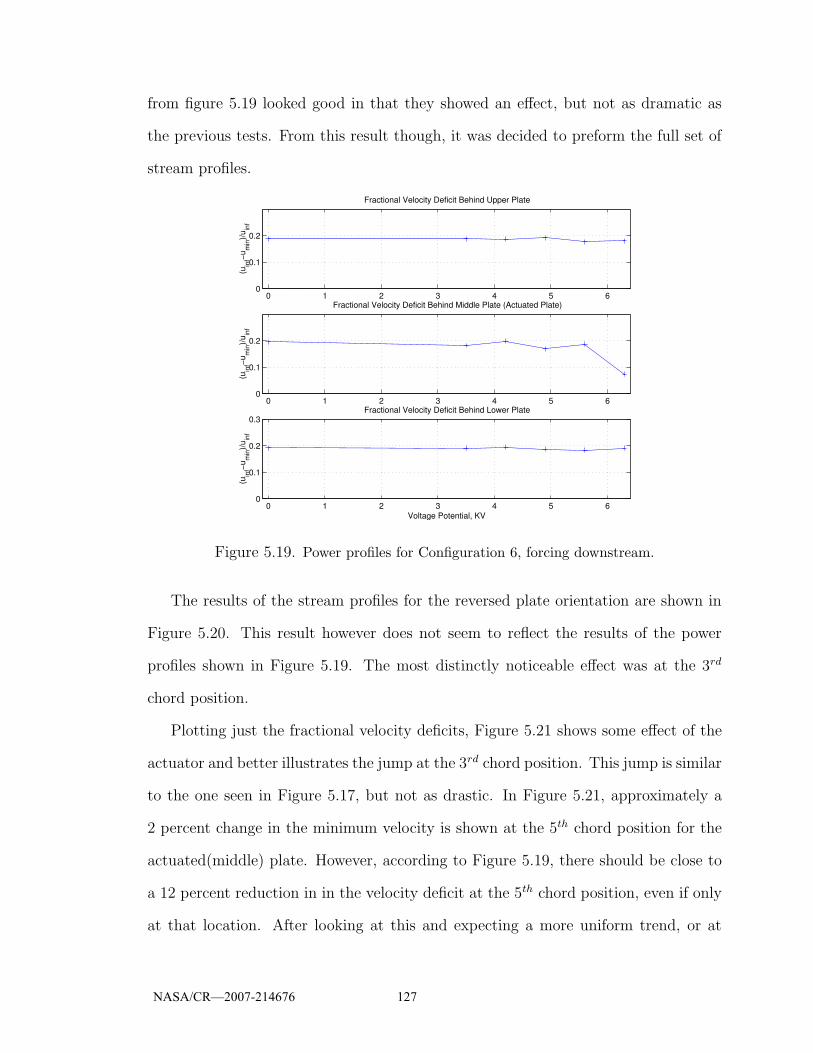
from figure 5.19 looked good in that they showed an effect, but not as dramatic as
the previous tests. From this result though, it was decided to preform the full set of
stream profiles.
0 1 2 3 4 5 60
0.1
0.2(u
inf−u
min
)/uin
f
Fractional Velocity Deficit Behind Upper Plate
0 1 2 3 4 5 60
0.1
0.2
(uin
f−um
in)/u
inf
Fractional Velocity Deficit Behind Middle Plate (Actuated Plate)
0 1 2 3 4 5 60
0.1
0.2
0.3
Voltage Potential, KV
(uin
f−um
in)/u
inf
Fractional Velocity Deficit Behind Lower Plate
Figure 5.19. Power profiles for Configuration 6, forcing downstream.
The results of the stream profiles for the reversed plate orientation are shown in
Figure 5.20. This result however does not seem to reflect the results of the power
profiles shown in Figure 5.19. The most distinctly noticeable effect was at the 3rd
chord position.
Plotting just the fractional velocity deficits, Figure 5.21 shows some effect of the
actuator and better illustrates the jump at the 3rd chord position. This jump is similar
to the one seen in Figure 5.17, but not as drastic. In Figure 5.21, approximately a
2 percent change in the minimum velocity is shown at the 5th chord position for the
actuated(middle) plate. However, according to Figure 5.19, there should be close to
a 12 percent reduction in in the velocity deficit at the 5th chord position, even if only
at that location. After looking at this and expecting a more uniform trend, or at
NASA/CR—2007-214676 127

0.6 0.8 1
−1
−0.5
0
0.5
1
u/uinf
0.5c
0.6 0.8 1
−1
−0.5
0
0.5
1
u/uinf
1c
0.6 0.8 1
−1
−0.5
0
0.5
1
u/uinf
2c
0.6 0.8 1
−1
−0.5
0
0.5
1
u/uinf
3c
0.6 0.8 1
−1
−0.5
0
0.5
1
u/uinf
4c
0.6 0.8 1
−1
−0.5
0
0.5
1
u/uinf
y/c
5c
OffOn
Figure 5.20. Stream profiles for Configuration 6, forcing downstream.
least again lacking the jump at the 3rd chord location, it was decided to repeat this
set of stream profiles.
The repeated stream profiles are shown in Figure 5.22. This case was noticeably
different in that the jump seen at the 3rd chord position was not there and, for the
actuated cases, the peaks decayed less rapidly than the unactuated cases. Also present
in these profiles, in particular at the 3rd and 5th chord positions, the middle peaks
show some flattening and erratic behavior. The fact that the peaks for the actuated
case decayed less rapidly in this experiment is not completely unexpected. It stands
to reason that reversing the direction of the forcing could reverse the effect.
As was done with the upstream forcing case, the repeated results were plotted
against the initial results. These are shown in Figure 5.23. As opposed to the up-
stream forcing setup, the base cases shown here are almost indistinguishable in the
figure. But again, the effect of the actuator was not consistent for the two tests after
the 3rd chord position. The actuator effect for the second test seemed more consis-
NASA/CR—2007-214676 128
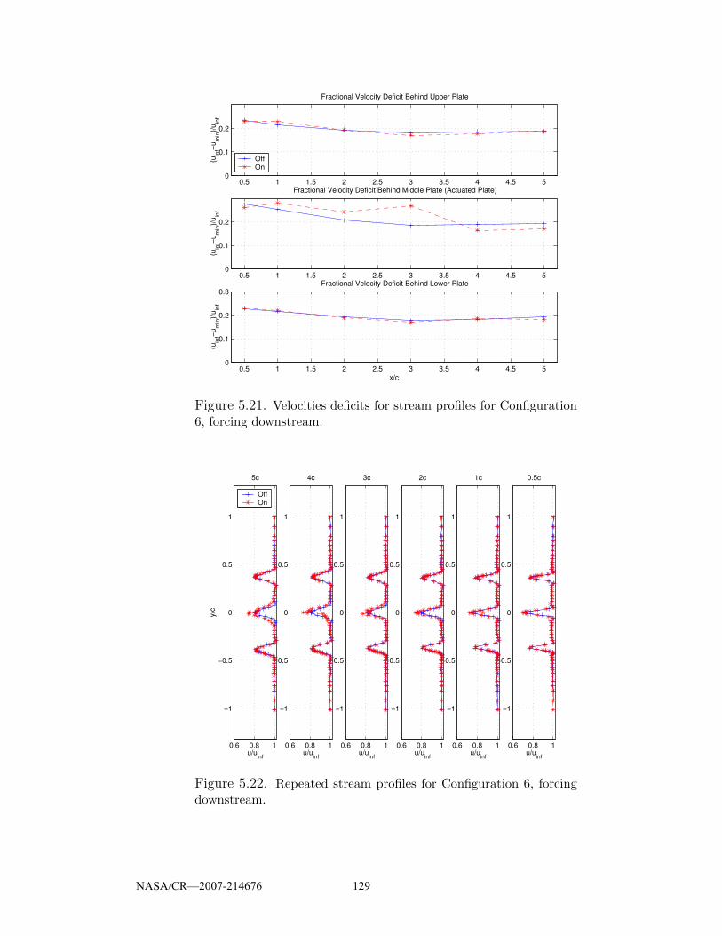
0.5 1 1.5 2 2.5 3 3.5 4 4.5 50
0.1
0.2
(uin
f−um
in)/u
inf
Fractional Velocity Deficit Behind Upper Plate
OffOn
0.5 1 1.5 2 2.5 3 3.5 4 4.5 50
0.1
0.2(u
inf−u
min
)/uin
f
Fractional Velocity Deficit Behind Middle Plate (Actuated Plate)
0.5 1 1.5 2 2.5 3 3.5 4 4.5 50
0.1
0.2
0.3
x/c
(uin
f−um
in)/u
inf
Fractional Velocity Deficit Behind Lower Plate
Figure 5.21. Velocities deficits for stream profiles for Configuration6, forcing downstream.
0.6 0.8 1
−1
−0.5
0
0.5
1
u/uinf
0.5c
0.6 0.8 1
−1
−0.5
0
0.5
1
u/uinf
1c
0.6 0.8 1
−1
−0.5
0
0.5
1
u/uinf
2c
0.6 0.8 1
−1
−0.5
0
0.5
1
u/uinf
3c
0.6 0.8 1
−1
−0.5
0
0.5
1
u/uinf
4c
0.6 0.8 1
−1
−0.5
0
0.5
1
u/uinf
y/c
5c
OffOn
Figure 5.22. Repeated stream profiles for Configuration 6, forcingdownstream.
NASA/CR—2007-214676 129

tent in terms of the decay trend, but the result was still not consistent with the first
power profile. The first power profile suggested a 12 percent decrease in the minimum
velocity at this point, not a 6 percent increase.
0.5 1 1.5 2 2.5 3 3.5 4 4.5 50
0.1
0.2
0.3
(uin
f−um
in)/u
inf
Fractional Velocity Deficit Behind Upper Plate
Test 1 OffTest 1 OnTest 2 OffTest 2 On
0.5 1 1.5 2 2.5 3 3.5 4 4.5 50
0.1
0.2
0.3
(uin
f−um
in)/u
inf
Fractional Velocity Deficit Behind Middle Plate (Actuated Plate)
0.5 1 1.5 2 2.5 3 3.5 4 4.5 50
0.1
0.2
0.3
x/c
(uin
f−um
in)/u
inf
Fractional Velocity Deficit Behind Lower Plate
Figure 5.23. Comparison of two wake decay tests using for Config-uration 6, forcing downstream.
Due to these inconsistencies, the first set of power profiles for this setup were
repeated. The repeated power profiles were plotted along with the first set and are
shown in Figure 5.24. From this it is apparent that the first set of results do not seem
to be repeatable, with the second set of results being more consistent with the results
seen in the stream profiles. As with the forcing upstream experiments, based on the
inconsistencies found in these results, it was decided that this plate orientation was
also to sensitive to work with and was abandoned. This was the last configuration
tried.
NASA/CR—2007-214676 130
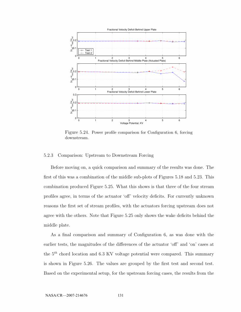
0 1 2 3 4 5 60
0.1
0.2
(uin
f−um
in)/u
inf
Fractional Velocity Deficit Behind Upper Plate
Test 1Test 2
0 1 2 3 4 5 60
0.1
0.2(u
inf−u
min
)/uin
f
Fractional Velocity Deficit Behind Middle Plate (Actuated Plate)
0 1 2 3 4 5 60
0.1
0.2
0.3
Voltage Potential, KV
(uin
f−um
in)/u
inf
Fractional Velocity Deficit Behind Lower Plate
Figure 5.24. Power profile comparison for Configuration 6, forcingdownstream.
5.2.3 Comparison: Upstream to Downstream Forcing
Before moving on, a quick comparison and summary of the results was done. The
first of this was a combination of the middle sub-plots of Figures 5.18 and 5.23. This
combination produced Figure 5.25. What this shows is that three of the four stream
profiles agree, in terms of the actuator ‘off’ velocity deficits. For currently unknown
reasons the first set of stream profiles, with the actuators forcing upstream does not
agree with the others. Note that Figure 5.25 only shows the wake deficits behind the
middle plate.
As a final comparison and summary of Configuration 6, as was done with the
earlier tests, the magnitudes of the differences of the actuator ‘off’ and ‘on’ cases at
the 5th chord location and 6.3 KV voltage potential were compared. This summary
is shown in Figure 5.26. The values are grouped by the first test and second test.
Based on the experimental setup, for the upstream forcing cases, the results from the
NASA/CR—2007-214676 131

0.5 1 1.5 2 2.5 3 3.5 4 4.5 50
0.05
0.1
0.15
0.2
0.25
0.3
x/c
(uin
f−um
in)/u
inf
Fractional Velocity Deficit Behind Actuated Plate
Forcing up − Test 1 OffForcing up − Test 1 OnForcing up − Test 2 OffForcing up − Test 2 OnForcing down − Test 1 OffForcing down − Test 1 OnForcing down − Test 2 OffForcing down − Test 2 On
Figure 5.25. Velocity deficits behind actuated (middle) plate for thetwo upstream and two downstream forcing cases.
power and stream profiles should match. The same goes for the downstream forcing
case. Obviously from this figure they do not agree. Averaging the four results for the
upstream case give a mean of 0.108 with a standard deviation of 0.045. This standard
deviation is approximately 3.5 times greater than what was seen with Configuration 5,
which had a comparably sized mean. The calculations of the downstream case gives a
mean of 0.053 with a standard deviation of 0.054. Having a standard deviation greater
than the mean is a good indication of how erratic the experimental values were. The
main thing to take from this is that these results were very inconsistent. This brings
up the issue of repeatability. If the apparatus can not perform consistently, it is
not useful as an experimental device. So, as mentioned before, these setups were
abandoned.
NASA/CR—2007-214676 132
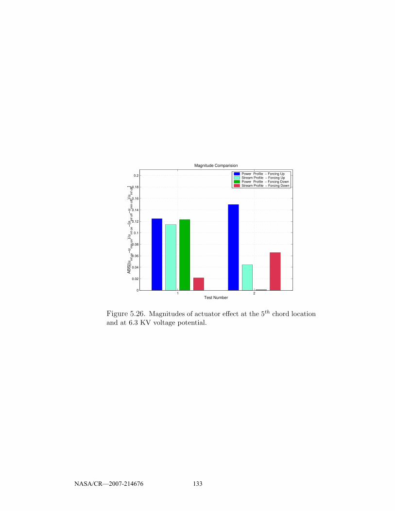
1 20
0.02
0.04
0.06
0.08
0.1
0.12
0.14
0.16
0.18
0.2
AB
S[(u
inf o
n−um
in o
n)/uin
f on−(
u inf o
ff−um
in o
ff)/uin
f off]
Test Number
Magnitude Comparision
Power Profile − Forcing UpStream Profile − Forcing UpPower Profile − Forcing DownStream Profile − Forcing Down
Figure 5.26. Magnitudes of actuator effect at the 5th chord locationand at 6.3 KV voltage potential.
NASA/CR—2007-214676 133

CHAPTER 6
RESULTS: DISCUSSION
In this chapter, comparisons of some of the different hot-wire measurements, for
the different configurations, will be presented. This is done to better illustrate some
of the findings and to point out which configurations worked and in what way they
worked.
6.1 Leading Edge Dependence
First to be presented are some results that discuss the leading edge dependence.
This is done mostly to draw attention to the variations found in the experimental data
that resulted from changing the leading edge. To illustrate the differences, the single
plate cases that were compared with Configurations 4 and 5 will be compared to each
other. Then, comparisons of both the single plate case to Configuration 4, which had
two plates with the 1/4 elliptic leading edge and one plate with the round leading
edge, and to Configuration 5, which had three plates with round leading edges.
A direct comparison of the effect of the leading edges can be made by plotting
the results for the two single plates. This comparison is shown in Figure 6.1. With
the exception of the 1/2 and 4th chord positions, the decay trends of the cases with
the plasma actuator off are very similar. However, there is a stark contrast between
the plasma on cases for the two airfoils. The 1/4 elliptic leading edge, in conjunction
with the plasma actuator, seems to work to hinder the turbulent mixing in the wake,
NASA/CR—2007-214676 134

thus increasing the time, which in turn increases the downstream distance for the
fractional velocity deficit to approach the free-stream value. Contrarily, the rounded
leading edge, in conjunction with the plasma actuator, seems to increase the wake
mixing, thus helping the velocity deficit to decrease.
0.5 1 1.5 2 2.5 3 3.5 4 4.5 50.05
0.1
0.15
0.2
0.25
0.3
x/c
(uin
f−um
in)/u
inf
Single Plate Comparision
Eliptical LE offEliptical LE onRound LE offRound LE on
Figure 6.1. Direct comparison of single plate with 1/4 elliptic lead-ing edge to a single plate with a round leading edge.
The results shown in the middle subplot of Figure 4.30 in Section 4.4, were re-
plotted in the the top subplot of Figure 6.2. This shows a comparison of a single
plate, with an 1/4 elliptic leading edge, to Configuration 4. Recall that Configura-
tion 4 had two plates with 1/4 elliptic leading edges and one plate, on the end, with
a round leading edge. Also, that the plate with the plasma actuator was the same
plate used for the single plate test, and the Configuration 4 test, compared in the
figure, thus both had 1/4 elliptic leading edges. Because the results for the plates
with the plasma actuators were the primary interest, only those will be compared.
The bottom subplot of Figure 6.2, shows the comparison of the same single plate case
to the actuated plate of Configuration 5. Recall that the plates in Configuration 5
NASA/CR—2007-214676 135
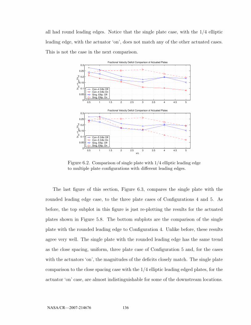
all had round leading edges. Notice that the single plate case, with the 1/4 elliptic
leading edge, with the actuator ‘on’, does not match any of the other actuated cases.
This is not the case in the next comparison.
0.5 1 1.5 2 2.5 3 3.5 4 4.5 50
0.05
0.1
0.15
0.2
0.25
0.3
(uin
f−um
in)/u
inf
Fractional Velocity Deficit Comparison of Actuated Plates
Con−4 3/8c OffCon−4 3/8c OnSing. Ellip. OffSing. Ellip. On
0.5 1 1.5 2 2.5 3 3.5 4 4.5 50
0.05
0.1
0.15
0.2
0.25
0.3
x/c
(uin
f−um
in)/u
inf
Fractional Velocity Deficit Comparison of Actuated Plates
Con−5 3/8c OffCon−5 3/8c OnSing. Ellip. OffSing. Ellip. On
Figure 6.2. Comparison of single plate with 1/4 elliptic leading edgeto multiple plate configurations with different leading edges.
The last figure of this section, Figure 6.3, compares the single plate with the
rounded leading edge case, to the three plate cases of Configurations 4 and 5. As
before, the top subplot in this figure is just re-plotting the results for the actuated
plates shown in Figure 5.8. The bottom subplots are the comparison of the single
plate with the rounded leading edge to Configuration 4. Unlike before, these results
agree very well. The single plate with the rounded leading edge has the same trend
as the close spacing, uniform, three plate case of Configuration 5 and, for the cases
with the actuators ‘on’, the magnitudes of the deficits closely match. The single plate
comparison to the close spacing case with the 1/4 elliptic leading edged plates, for the
actuator ‘on’ case, are almost indistinguishable for some of the downstream locations.
NASA/CR—2007-214676 136
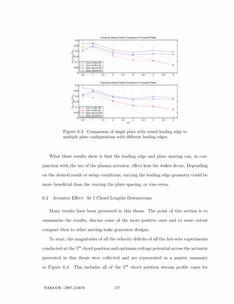
0.5 1 1.5 2 2.5 3 3.5 4 4.5 50
0.05
0.1
0.15
0.2
0.25
0.3
(uin
f−um
in)/u
inf
Fractional Velocity Deficit Comparison of Actuated Plates
Con−5 3/8c OffCon−5 3/8c OnSing. Round OffSing. Round On
0.5 1 1.5 2 2.5 3 3.5 4 4.5 50
0.05
0.1
0.15
0.2
0.25
0.3
x/c
(uin
f−um
in)/u
inf
Fractional Velocity Deficit Comparison of Actuated Plates
Con−4 3/8c OffCon−4 3/8c OnSing. Round OffSing. Round On
Figure 6.3. Comparison of single plate with round leading edge tomultiple plate configurations with different leading edges.
What these results show is that the leading edge and plate spacing can, in con-
junction with the use of the plasma actuator, effect how the wakes decay. Depending
on the desired result or setup conditions, varying the leading edge geometry could be
more beneficial than the varying the plate spacing, or vise-versa.
6.2 Actuator Effect: At 5 Chord Lengths Downstream
Many results have been presented in this thesis. The point of this section is to
summarize the results, discuss some of the more positive ones and to some extent
compare then to other moving-wake generator designs.
To start, the magnitudes of all the velocity deficits of all the hot-wire experiments
conducted at the 5th chord position and optimum voltage potential across the actuator
presented in this thesis were collected and are represented in a master summary
in Figure 6.4. This includes all of the 5th chord position stream profile cases for
NASA/CR—2007-214676 137

Configurations 3 through 6 and the two single plate cases. Also, this figure includes
all of the power profiles done at the optimum voltage for Configurations 4 through
6. Below the figure is a table that contains a summary of the experimental setup
corresponding to the number designation shown in the figure. The summary table
contains the designation number, configuration number, angle of attack of the plate,
the chord spacing of the plates, the profile type, voltage potential of the test and
notes where needed.
A final comparison of results at the 5th chord location are shown in Figure 6.5.
This shows the mean and standard deviation, where possible, of similar test cases that
were presented in the master summary. Only select setups of interest are presented.
In the table under the figure, there is a column labeled ‘Master Desig.’. This is a list of
the data points used that correspond to the Master Designation list from Figure 6.4 in
the calculation of the mean and standard deviation. The results discussed in Section
4.2.2 illustrate why Master Designations 3,4, and 5 could be averaged, though the
setups where not exactly the same. With the other averages, the only things different
between the points was the day the test was done and whether it was a stream or
power profile. All other test conditions such as the configuration, orientation, spacing,
and power supplied were all the same. This figure, along with the table, collectively
shows what worked at the 5th chord location. Some of advantages and disadvantages
of the different setups will be discussed next.
Clearly from Figure 6.5 Designation 1 was the most effective and most repeatable
setup. However, caution has to brought to the voltage potential needed to each this
affect. Also attention should made to having the plates turned, the location of the
minimum velocities for the ‘off’ and ‘on’ cases will not be the same, nor will they
be in line with the plate, whereas for the zero angle of attack cases, the peaks are
in line with each other and the plate. Recall that the 11.2 KV potential was chosen
NASA/CR—2007-214676 138
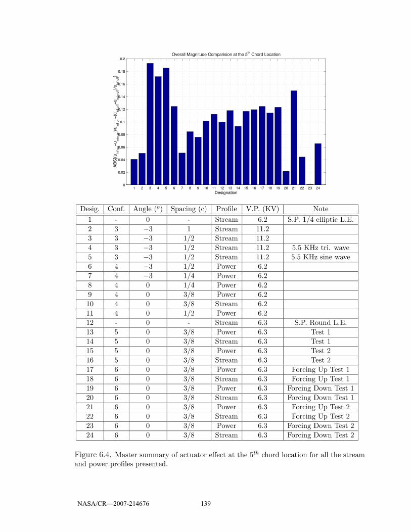
1 2 3 4 5 6 7 8 9 10 11 12 13 14 15 16 17 18 19 20 21 22 23 240
0.02
0.04
0.06
0.08
0.1
0.12
0.14
0.16
0.18
0.2
AB
S[(u
inf o
n−um
in o
n)/uin
f on−(
u inf o
ff−um
in o
ff)/uin
f off]
Designation
Overall Magnitude Comparision at the 5th Chord Location
Desig. Conf. Angle (o) Spacing (c) Profile V.P. (KV) Note
1 - 0 - Stream 6.2 S.P. 1/4 elliptic L.E.
2 3 −3 1 Stream 11.2
3 3 −3 1/2 Stream 11.2
4 3 −3 1/2 Stream 11.2 5.5 KHz tri. wave
5 3 −3 1/2 Stream 11.2 5.5 KHz sine wave
6 4 −3 1/2 Power 6.2
7 4 −3 1/4 Power 6.2
8 4 0 1/4 Power 6.2
9 4 0 3/8 Power 6.2
10 4 0 3/8 Stream 6.2
11 4 0 1/2 Power 6.2
12 - 0 - Stream 6.3 S.P. Round L.E.
13 5 0 3/8 Power 6.3 Test 1
14 5 0 3/8 Stream 6.3 Test 1
15 5 0 3/8 Power 6.3 Test 2
16 5 0 3/8 Stream 6.3 Test 2
17 6 0 3/8 Power 6.3 Forcing Up Test 1
18 6 0 3/8 Stream 6.3 Forcing Up Test 1
19 6 0 3/8 Power 6.3 Forcing Down Test 1
20 6 0 3/8 Stream 6.3 Forcing Down Test 1
21 6 0 3/8 Power 6.3 Forcing Up Test 2
22 6 0 3/8 Stream 6.3 Forcing Up Test 2
23 6 0 3/8 Power 6.3 Forcing Down Test 2
24 6 0 3/8 Stream 6.3 Forcing Down Test 2
Figure 6.4. Master summary of actuator effect at the 5th chord location for all the streamand power profiles presented.
NASA/CR—2007-214676 139

1 2 3 4 50
0.02
0.04
0.06
0.08
0.1
0.12
0.14
0.16
0.18
0.2
AB
S[(u
inf o
n−um
in o
n)/uin
f on−(
u inf o
ff−um
in o
ff)/uin
f off]
Designation
Final Magnitude Comparision
meanstd
Desig. Conf. Angle (o) Spacing (c) V.P. (KV) Master Desig.#’s Used in Average
1 3 −3 1/2 11.2 3,4,5
2 4 0 3/8 6.2 9,10
3 5 0 3/8 6.3 13,14,15,16
4 6 0 3/8 6.3 17,18,21,22
5 6 0 3/8 6.3 19,20,23,24
Figure 6.5. Comparison of similar results at the 5th chord location to magnitude andrepeatability of the actuator effect.
NASA/CR—2007-214676 140

because while performing the flow visualization, it appeared to be the most effective.
Referring back to Figure 6.4, the change from Configuration 3 to Configuration 4, is
shown by Designation 6, illustrates approximately a 6 percent decrease in the actuator
affect caused by the reduction of power and the addition of the third plate. However,
it is unclear at this time the degree that the power reduction and third plate addition
individually had. However, based on the differences in flow visualization results shown
in Figure 4.7 and Figure 4.10, it seems that the reduction in the effect is primarily
dependent on the change in voltage. Recall that the difference seen in the flow
visualization occurred from increasing the voltage potential from 8.4 KV to 11.2 KV.
Of the remaining points, in Figure 6.5, Designation 3 is best configuration. It
shows the highest velocity variation between the plasma actuator ‘off’ and ‘on’ cases,
with the smallest standard deviation. This configuration has the advantage in that
it requires less power, but as noted before, this may not be entirely the case when
compared to Designation 1. Also, geometrically, a zero angle of attack setup would
be easier to construct. However, the wider spacing angle of attack cases appear to be
less sensitive to small geometrical variations.
Lastly, as pointed out before, Configuration 6, shown by Designations 4 and 5 in
Figure 6.5, is the worst choice. This configuration had the highest standard deviation
of the data points, which brings to question the repeatability of the results. Affects of
the moving-wake generator on the flow have to be know and consistent to be used as
a practical tool. These inconsistencies show that this configuration does not adhere
to this requirement.
Given the original design constraint of 10.0 in. (25.4 cm), which for the plates was
5 chord lengths, the 1/2 chord, −3o angle of attack, 11.2 KV potential of Configuration
3 and 6.3 KV potential case of Configuration 5 worked the best. These results are
comparable to Doorly’s setup which achieved 10 to 20 percent velocity fluctuations[6]
NASA/CR—2007-214676 141
but lower than the 25 percent variation reported by Murawski and Vafai[15], which
was based on results of Halstead et al.[12]. It is unclear whether the 25 percent
estimate is based on the physical distance between the plain of the test blade leading
edges and the plain of the cylinder motion or based on the distance in the wake
path. The wake path distance is always greater than the physical distance between
the plains, due to the geometry of the setup, and is dependent on the cylinder and
free-stream velocities. The point being that the 25 percent could an over-estimate
based on wake path distance. For the present work the wake path distance has not
been considered because attempts at propagating the disturbance were not made.
The next section discusses the feasibility of positioning the moving-wake generator,
based on current results presented in the this thesis, to distances on the order of one
chord from the test blades.
6.3 Actuator Effect: At Other Chord Lengths Downstream
In this section, some of the results for the 1/2 and 1 chord downstream positions
will be presented to illustrate some flexibility in the application of the unsteady
turbulence generator. Up till now, the results shown have been restricted to the 5th
chord position design constraint. This constraint was placed on the design for the
first intended application. Other researchers may have different design requirements.
The only data available for this investigation is from the stream profiles. As was
done before, the magnitudes of the velocity deficits for the 1/2 and 1 chord location
were collected and are presented in Figure 6.6. This bar graph shows that positioning
the moving-wake generator closer to the test blades has no benefit. However, these
data points where collected as the previous ones, that is, at a fixed position, in
line with the minimum velocity of the actuator ‘off’ case for the 1/2 chord location
profile, behind the actuated plate. For the cases of the −3o angle of attack, if the
NASA/CR—2007-214676 142

measurement location is shifted, there is an improvement.
The motivation for investigating the closer chord positions is due to the large
difference between the plasma actuator ‘off’ and ‘on’ case at the 1 chord plate spacing,
−3o angle of attack, tests of Configuration 3 at the 1/2 chord downstream location.
Select mean velocity profiles, from the stream profiles for that setup shown in Figure
4.13 of Section 4.2.2 were replotted, along with the difference between the ‘off’ an
‘on’ case shifted, by adding 1 to all the values. This was done so that all three sets of
data could be on the same axis and the result of this is shown as Figure 6.7. Included
in the first sub-plot is a sketch reflecting the plate orientation and location that the
data was taken. The horizontal line indicated by the letter ‘A’ is the location of
minimum velocity of the actuator ‘off’ case, and thus the y-location where the data
was taken for comparison in the previous bar graphs. The horizontal line indicated
by the letter ‘B’ is in line with the center of the plate. The line indicated by the letter
‘C’ represents the angle of attack of the plate and the projected area. The vertical
distance between the ends of this line are drawn to scale with the actual width of the
projected area of the plate. The length, angle, or the location of the line in no other
way represent the actual location of the plate.
Obviously from Figure 6.7, the values used for comparison where not at the lo-
cation of the maximum velocity deficit. This is due to the angle of attack of the
plate. Since the angle of attack is small, the flow stays attached as it goes around the
plates. This shifts the location of the minimum velocity above the physical location
of the plate. When the plasma actuator is turned ‘on’, the induced velocity causes
the flow to at least partially separate from the low pressure side of the plate. This in
turn makes plate appear more like a bluff body. Which is why the wake shifts down
towards the centerline of the plate. Recall that the flow visualization images shown
in Figure 4.10 illustrated the large scale vortex shedding. For this case, the maximum
NASA/CR—2007-214676 143

1 2 3 4 5 6 7 8 9 10 11 12 130
0.02
0.04
0.06
0.08
0.1
0.12
0.14
0.16
0.18
0.2
AB
S[(u
inf o
n−um
in o
n)/uin
f on−(
u inf o
ff−um
in o
ff)/uin
f off]
Designation
Overall Magnitude Comparision
1/2 chord downstream 1 chord downstream
Desig. Conf. Angle (o) Spacing (c) Profile V.P. (KV) Note
1 3 −3 1 Stream 11.2
2 3 −3 1/2 Stream 11.2
3 3 −3 1/2 Stream 11.2 5.5 KHz
4 3 −3 1/2 Stream 11.2 5.5KHz sine wave
5 4 0 3/8 Stream 6.2
6 5 0 3/8 Stream 6.3 Test 1
7 5 0 3/8 Stream 6.3 Test 2
8 - 0 - Stream 6.2 S.P. 1/4 Elliptic LE
9 - 0 - Stream 6.3 S.P. Round LE
10 6 0 3/8 Stream 6.3 Forcing Up Test 1
11 6 0 3/8 Stream 6.3 Forcing Down Test 1
12 6 0 3/8 Stream 6.3 Forcing Up Test 2
13 6 0 3/8 Stream 6.3 Forcing Down Test 2
Figure 6.6. Summary of actuator effect at the 1/2 and 1 chord locations for all of thestream profile cases.
NASA/CR—2007-214676 144
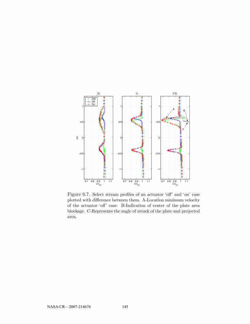
0.7 0.8 0.9 1 1.1
−1
−0.5
0
0.5
1
u/uinf
0.5c
0.7 0.8 0.9 1 1.1
−1
−0.5
0
0.5
1
u/uinf
1c
0.7 0.8 0.9 1 1.1
−1
−0.5
0
0.5
1
u/uinf
y/c
5c
Diff.OffOn
A B
C
Figure 6.7. Select stream profiles of an actuator ‘off’ and ‘on’ caseplotted with difference between them. A-Location minimum velocityof the actuator ‘off’ case. B-Indication of center of the plate areablockage. C-Represents the angle of attack of the plate and projectedarea.
NASA/CR—2007-214676 145

fluctuation at the 1/2 chord location is 27 percent of the free-stream and drops to
roughly 15 percent and 8 percent at the 1st and 5th chord location respectively.
Similarly, Figure 6.8, shows the same type of illustration for the −3o, 1/2 chord
spacing case of Configuration 3. This time only the difference is shown. Because of
this, it did not have to be shifted. The corresponding stream profiles for this case were
shown in Figure 4.14 in Section 4.2.2. This figure shows that the presented results for
the −3o, 1/2 chord spacing cases of Configuration 3, at the 5th chord location, where
close to there maximum amplitudes. The highest magnitude was approximately 31
percent at the 1/2 downstream position.
−0.4 −0.2 0 0.2
−1
−0.5
0
0.5
1
(uoff
/uinf off
)−(uon
/uinf on
)
0.5c
−0.4 −0.2 0 0.2
−1
−0.5
0
0.5
1
(uoff
/uinf off
)−(uon
/uinf on
)
1c
−0.4 −0.2 0 0.2
−1
−0.5
0
0.5
1
y/c
(uoff
/uinf off
)−(uon
/uinf on
)
5c
Figure 6.8. Difference between actuator ‘off’ and ‘on’ case for −3o,1/2 chord spacing case of configuration 3. A-Location minimumvelocity of the actuator ‘off’ case. B-Indication of center of the platearea blockage. C-Represents the angle of attack of the plate andprojected area.
Some additional remarks will be made in Chapter 7 discussing some recommen-
dations that would investigate the possible versatility of the moving-wake generator
as alluded to in Figures 6.7 and 6.8.
NASA/CR—2007-214676 146

CHAPTER 7
CONCLUSIONS AND RECOMMENDATIONS
Presented in this chapter are some conclusions and recommendations for future
work, both coupled with some final remarks. The chapter is broken down in to those
two sub-sections.
7.1 Conclusions
The main objective of the work presented in this thesis was a proof of concept of
the ability to use plasma actuators as an moving-wake generator. Many steps were
taken to achieve this objective with promising results. The results of the experiments
are concluded here.
Mean velocity profiles using a hot-wire were conducted in the wake of an unac-
tuated NACA 0018 airfoil at the following downstream chord locations; 1/2, 1, 2, 3,
4, and 5 chord lengths. These tests were done at two velocities, namely 31 ft/s (9.45
m/s) and 54 ft/s (16.5 m/s). Similarity plots of the wake showed good agreement
with theory in terms of the wake width and velocity deficit. The same tests were
performed on two NACA 0018 airfoils to test the wake interactions relative to the
airfoil spacing. It was shown that for a free-stream velocity of 31 ft/s (9.45 m/s) and
a blade spacing of 1/3 chord that the airfoil wakes never act independently. For a
spacing of 2/3 chord at the same velocity, the wakes started to interact 1 chord length
downstream. At the last spacing, 1 chord length, the wakes were independent through
NASA/CR—2007-214676 147
the 5 chord lengths. Similarly for the 54 ft/s (16.5 m/s) velocity, 1/3 chord spacing
case, the wakes were never independent. For the 2/3 chord spacing, the wakes started
to interact between 1 and 2 chord lengths downstream and for the 1 chord spacing
case, the wakes were again independent throughout the 6 streamwise locations.
Plasma actuators with a 0.5 in. (1.27 cm) wide upper and lower electrode, were
tested at three different chord positions on one of the two NACA 0018 airfoils at a
voltage potential of 12.5 KV. The actuator was placed such that the active edge was at
the 25 percent chord location and forcing the flow upstream. While the airfoil spacing
was fixed at a 2/3 chord length, additional chord positions of 27 and 30 percent were
tested with the 27 percent chord location, also the point of maximum thickness of
the airfoil, being the most effective. This conclusion was based on flow visualization
results. Also from these, the actuator/airfoil setup did not appear to have enough of
an effect on the flow to use for the moving-wake generator.
Flow visualization techniques were also implemented for the study of two flat
plates at zero angle of attack with plasma actuators that used Kapton tape as the
dielectric material. Various actuator positions including the leading edge and 0.125
in. (0.318 cm) from the leading edge were tested, in addition to having multiple
numbers of actuators in an array on both plates. Also, plate spacings of 1/4, 3/8,
and 1/2 chord where tested. All these setups were tried at voltages levels of 1.9 and
6.8 KV potentials but showed no real affect.
The two plates were also tried at various angles of attack between 0 and 16 degrees
with a plasma actuator positioned at the leading edge using a voltage potential of 11.2
KV. Flow visualization showed that the actuator could reattach the separated flow at
the higher angle-of-attack cases, and thus be able to cause an unsteady disturbance
by turning the actuator ‘on’ and ‘off’. All of these tests were conducted at a plate
spacing of 1 chord length. Limitations in the adhesive of the copper tape and the
NASA/CR—2007-214676 148

robustness of the Kapton tape made it impossible to complete velocity profiles using
a hot-wire due to the plasma actuator failing. Because of this, the dielectric material
was changed to FR-4 printed circuit board material. Doing this also forced a change
in the actuator location. The FR-4 printed circuit board material proved to be a much
better dielectric material. The plasma actuators using it could be run intermittently
for hours at a time and actuators could last for days of testing.
Tests with the active edge of the plasma actuator at the mid-chord of the plate,
with the two plates at -3, -5, and -7 degrees angle of attack, at 1 chord spacing, with
a voltage potential of 11.2 KV were very positive. For these tests, the actuator forced
the flow upstream in the channel between the plates and downstream on the opposite
side of the actuated plate. Flow visualization showed very high levels or turbulence
in the wake, implying the ability of the plasma actuator to separate the flow from
the low-pressure side of the plate. Based on the flow visualization, the −3o angle
of attack case was chosen for hot-wire measurements. The hot-wire measurements
showed velocity fluctuations as large as 27, 16, and 8 percent of the free-stream
velocity could be produced at the 1/2, 1, and 5 chord length downstream locations,
respectively. Note that the plates used for these test had a 1/4 elliptical leading edge
sloping away from the lower electrode. By reducing the spacing to 1/2 chord length,
the possible velocity fluctuations were increased to as large as 31, 20, and 22 percent
of the free-stream velocity at the respective 1/2, 1, and 5 chord downstream locations.
The combination of adding a third plate, one now on each side of the plate with
the plasma actuator, and reducing the voltage potential across the actuator to 6.2
KV but maintaining the −3o angle of attack and 1/2 chord spacing, caused an ap-
proximately 6 percent, of the free-stream velocity, decrease in the magnitude of the
velocity fluctuation. Moving the plates closer together to 1/4 chord spacing caused
an additional 7 percent decrease in effectiveness to approximately 5 percent of the
NASA/CR—2007-214676 149

free-stream at the 5th downstream chord location.
A non-uniform set of three plates and a uniform set of three plates were tested at
zero angle of attack and 3/8 chord spacing. The uniform set of plates proved to give
slightly better results, varying between approximately 9.7 to 12 percent, as opposed
to 7.8 to 10 percent for the non-uniform plates, of the free-stream velocity at the 5th
downstream chord position. This was the location of the greatest affect for the zero
angle of attack cases.
Tests with a sandwiched plate design that allowed the plasma actuator to force the
flow upstream or downstream on both sides of the plate at a 3/8 chord spacing gave
poor results. For the forcing upstream tests, the magnitude of the velocity fluctuation
ranged from approximately 4.1 to 15 percent. For the downstream cases, the values
ranged from close to zero to 12 percent at the 5th downstream chord position.
In addition to these tests, single plate experiments were done for comparative
purposes. Two single plates were tested at zero angle of attack; one had a round
leading edge and the other had with a 1/4 elliptic leading edge. The plate with round
leading was tested at a 6.3 KV voltage potential and proved to be 6 percent of the
free-stream velocity better than the 4 percent velocity fluctuation possible with the
plate with the 1/4 elliptic leading edge. This put the single plate with the round
leading edge close to the values, in terms of the possible velocity fluctuation, seen
with the zero angle of attack 3/8 chord uniform plate cases.
In conclusion, the two plate, −3o angle of attack, 1/2 chord spacing, 11.2 KV volt-
age potential case with the 1/4 elliptic leading edges proved to be the most affective
in terms of the magnitude fluctuations produced. The second most affective was the
zero degree angle of attack, 3/8 chord spacing, 6.3 KV voltage potential case with
the three uniform plates with the round leading edge.
The results presented in this thesis have shown the feasibility of the conceptual
NASA/CR—2007-214676 150
design for the moving-wake generator. Results comparable to currently implemented
designs have been achieved by two different test setups. Depending on design con-
straints and levels of turbulence desired, one of the two options could be better than
the other, as such, further investigations should be done to pick one over the other.
7.2 Recommendations for Future Work
The work presented in this thesis has built a good foundation towards achieving
a useful tool for turbine research. It has also raised some additional questions that
could be addressed before making a final choice between the two existing options
and finalizing a design. This section will present some of final comments on the two
options and the questions they pose.
The −3o, 1/2 chord spacing case that had the plates with the 1/4 elliptic leading
edge has been shown to produce the largest velocity fluctuation. Based on this alone
it would appear to be the best choice, but this effect was achieved at the 11.2 KV
potential. If a better dielectric materials can be found that can hold up to the stress
of these potentials this setup may be the better choice. In addition to the dielectric
material needed, the plasma generating system must be able to maintain those power
levels for extended periods of time, even for longer electrode lengths. Increasing the
size and length of the plasma actuator increases the current required. This in turn
increases the power required from the system. If system is not capable of outputting
more power, then the maximum achievable voltage potential decreases with the size of
the actuator which, for this setup, seems to decrease the magnitude of the achievable
velocity fluctuation. During the course of this thesis, advancements in the area of
power available by the system have been made but still need to be proven in this
application. This could be done by doing what was referred to as power profiles
behind this plate setup for voltage potentials over the range of 7 to 14 KV.
NASA/CR—2007-214676 151
The zero angle of attack case has the advantage in that it was shown that in-
creasing the voltage over the 6.3 KV did not improve the response of the flow. If
the velocity fluctuations on the order of 12 percent of the free-stream velocity are
acceptable, then the 3/8 chord zero angle of attack case with the uniform plates, that
had the round leading edge seems to be the best choice. However, one has to keep
in mind that because the cascade of turbine blades is going to be at an angle to the
moving-wake generator, the 12 percent fluctuation is only going to be for the test
blade that is 5 chord lengths from the moving-wake generator. Based on the results,
the closer blades would experience turbulence fluctuations of a smaller magnitude.
It is unclear at this point what the farther blades would experience, so the effect at
farther downstream chords positions should be investigated.
One over shadowing question that remains is which of the plate styles, in terms of
the leading edge, is the best. The answer to that question is lacking at least one test
case. For the zero angle of attack, 3/8 chord spacing tests the rounded leading edge
plates worked the best. The experiments at the −3o angle of attack were only done
with the plates with the 1/4 elliptic leading edge, so an angle of attack comparison,
incorporating the different leading edge geometries could not be made. To do this,
wake profiles need to be performed behind the plates with the round leading edge, at
least for the −3o angle of attack, 1/2 chord spacing, 11.2 KV test case.
An investigation that could remedy, in the event that it is a problem, the issue of
the blades experiencing different levels of turbulence due to the varying distances of
the blades from the moving-wake generator, would be to cant the array of the plates.
If the array of plates where angled such that the array is parallel to the cascade of the
turbine blades, while keeping the plates themselves parallel to the incoming flow, the
distances from the plates to the airfoils would be constant. Experiments of this setup
could prove to be beneficial, although, by canting the array, the amount of overlap of
NASA/CR—2007-214676 152

the plates decreases. This in turn could reduce the close spacing effects seen in the
results. It is worth investigating because canting the array would allow the plates to
be positioned much closer to the turbine blades and allow more flexibility.
A potential advantage of the −3o angled plate case is that the angle the plates
make with the flow could actually aid in the propagation of the disturbance across
the test section. This is because when the actuators are ‘off’, the flow is already
turning around the plate. Coupled with the contiguous firing of the actuators on
the different plates, this could prove to be very beneficial. In order to investigate
this, some two-dimensional velocity experiments could be done using PIV or LDV
technologies. As with the flat plates, putting these plates in a cascade of their own,
parallel to the test cascade, so that they could be placed closer to the leading edge of
the turbine blades could again prove to be beneficial, especially in being able to use
the plasma actuators to vary the inlet flow angle to the turbine cascade.
Also, an additional investigation of the already obtained data into the area of
the turbulence intensity between the plates needs to be done. The approach taken
was to place the test plates or airfoils as close together as possible but still have the
wakes act independently at 5 chord lengths downstream. As discussed earlier, the
stochastic turbulence levels caused by the mixing of the upper stages of the turbine
were on the order of 5 percent. It stands to reason then, instead of adding a turbulence
grid to create the turbulence, move the plates closer together to have the minimum
turbulence level between the wakes closer to 5 percent. The spacing required to do
this could again prove to be useful for a final design.
The plate spacings chosen were artificially constrained to have the wakes interact
as little as possible. This was done first intended application to minimize the affect of
the passive unit while still keeping the discreetness of the moving-wake to a minimum,
Doing this was also beneficial in that the closer spacings, which allowed the wakes
NASA/CR—2007-214676 153
to interact, lessened the magnitude of the obtainable velocity difference between the
actuator ‘off’ and ‘no’ case. A further investigation into the closer plate spacings
however has been recommend to couple this work with other experimental and com-
putational work being done at the University of Notre Dame. An advantage of the
moving-wake generator over mechanical means is that it can produce purely vortical
disturbances. All off the mechanical methods produce both vortical and potential
disturbances. For computational work it is important to decouple these disturbances.
This is because many computational programs utilize purely vortical disturbances as
their input parameter [13]. Developing the moving-wake such that the vortical distur-
bance can be know and controlled would be greatly beneficial so comparisons between
experimental and computational results could be made. This could be done because
the same input could be used for the experiment and the computation. Once the
computation is proven by the experimental result, it could then be used as a model
in turbine machinery design. Some references into the experimental effort in this area
by the University of Notre Dame are Fabian[8] and Falk[9, 10]. The computational
effort being done at the University of Notre Dame is being done by Atassi[2, 1, 11].
During the course of this thesis additional knowledge has been gained about the
role the electrode widths play. A study into the effect of shorting the upper electrode,
to enable the chord length of the plate to be reduced could prove to be advantageous,
especially if there is an intent to move the plates closer to the test blades of the turbine
cascade. Reducing the plate’s chord length could allow for shorter times scales for the
vortex shedding. Shorter plates may also prove to be beneficial for an investigation
of the closer spacings that may maybe needed for gearing the moving-wake generator
to validate computational work.
Many suggestions have been made for future work. In terms of getting a workable
piece of test equipment for the intended first application, many of them are not
NASA/CR—2007-214676 154

necessary. To find the best design, to have confidence that it is the best, and have it
catered specifically for a desired purpose then investigations into the suggested setups
and additional data reduction should be done.
Lastly, the moving-wake generator is not meant to replace full rotating test rigs.
It is a simulator meant to be used as an easy to implement tool to aid researchers in
performing experiments in controllable, but closer to real world, wind tunnel appli-
cations.
NASA/CR—2007-214676 155

BIBLIOGRAPHY
[1] Akai, T. J., and Atassi, H. M. “Aerodynamic and Aeroelastic Character-istics of Oscillating Loaded Cascades at Low Mach Number. Part I: PressureDistribution, Forces and Moments”. Journal of Engineering Power 102 (1980),344–351.
[2] Atassi, H. M., and Grzedzinski, J. “Unsteady Disturbances of StreamingMotions Around Bodies”. Journal of Fluid Mechanics 209 (1989), 385–403.
[3] Codner, D. I. “An Investigation of Combined Heat Exchanger/Turning VanesFor Wind Tunnels”. Master’s thesis, Illinois Insitute of Technology, December1986.
[4] Corke, Thomas C. and He, Chuan and Mehul P. Patel. “Plasma Flapsand Slats: An Application of Weakly-Ionized Plasma Actuators”. AIAA paper(2004-2127).
[5] Dibelius, G. H., and Ahlers, E. “Infulence of Periodically Unsteady WakeFolw on the Flow Separation in Blade Channels”. Journal of Turbomachinery114 (January 1992), 108,113.
[6] Doorly, D. J. “Modeling the Flow in a Turbine Rotor Passage”. Journal ofTurbomachinery 110 (January 1988), 27,37.
[7] Doorly, D. J., and Oldfield, M. L. G. “Simulation of Wake Passing ina Stationary Turbine Rotor Cascade”. Journal of Propulsion and Power 114(1985), 316,318.
[8] Fabian, M. K., and Jumper, E. J. “Convected and Potential UnsteadyDisturbances Interacting With an Unsteady Cascade”. AIAA paper, 96-2627(1996).
[9] Falk, E. A., Jumper, E. J., and Fabian, M. K. “An Experimental Study ofUnsteady Forcing in the F109 Turbofan Engine”. AIAA paper, 97-3286 (1997).
[10] Falk, E. A., Jumper, E. J., Fabian, M. K., and Stermer, J. “Upstream-Propagating Potential Disturbances Interacting with a Compressible Cascade”.Journal of Propulsion and Power (2000).
[11] Fang, J., and Atassi, H. M. “Compressible Flows with Vortical Disturbancesaround a Cascade of Loaded Airfoils”. In Unsteady Aerodynamics, Aeroacoustics,and Aeroelasticity of Turbomachines and Propellers, H. M. Atassi, Ed. Springer-Verlag, New York, NY, 1993, pp. 149–176.
NASA/CR—2007-214676 156
[12] Halstead, D. E., Wisler, D. C., Okiishi, T. H., Walker, G. J., Hod-son, H. P., and Shin, H.-W. “Boundary Layer Development in Axial Com-pressord and Turbines Part 4 of 4: Computations and Analysis”. ASME PaperNo., 95-GT464 (1995).
[13] Jumper, E. “Internal collaboration at the University of Notre Dame”, June2004.
[14] Loehrke, R., and Nagib, H. M. “Experiments on Management of Free-Stream Turbulence”. Tech. Rep. 598, AGARD-R, September 1972.
[15] Murawski, C. G., and Vafai, K. “Effect of Wake Disturbance Frequency onthe Secondary Flow Vortex Structure in a Turbine Blade Cascade”. Journal ofFluids Engineering 122 (September 2000), 606,613.
[16] Pfeil, H., Herbst, R., and Schroder, T. “Investigation of the Laminar-Turbulent Transition of Boundary Layers Disturbed by Wakes”. Journal of En-gineering Power 105 (January 1983), 130,137.
[17] Post, M. L. “Phased Plasma Actuators for Unsteady Flow Control”. Master’sthesis, University of Notre Dame, July 2001.
[18] Post, M. L. “Plasma Actuators for Separation Control on Sationary and Os-cillating Wings”. PhD dissertation, University of Notre Dame, May 2004.
[19] Schobeiri, M. T., and Pappu, K. “Experimental Study on the Effect ofUnsteadiness on Boundary Layer Development on a Linaer Turbine Cascade”.Engineering in Fluids 114 (February 1997), 306,316.
NASA/CR—2007-214676 157
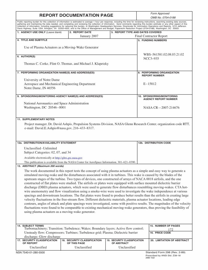
This publication is available from the NASA Center for AeroSpace Information, 301–621–0390.
REPORT DOCUMENTATION PAGE
2. REPORT DATE
19. SECURITY CLASSIFICATION OF ABSTRACT
18. SECURITY CLASSIFICATION OF THIS PAGE
Public reporting burden for this collection of information is estimated to average 1 hour per response, including the time for reviewing instructions, searching existing data sources,gathering and maintaining the data needed, and completing and reviewing the collection of information. Send comments regarding this burden estimate or any other aspect of thiscollection of information, including suggestions for reducing this burden, to Washington Headquarters Services, Directorate for Information Operations and Reports, 1215 JeffersonDavis Highway, Suite 1204, Arlington, VA 22202-4302, and to the Office of Management and Budget, Paperwork Reduction Project (0704-0188), Washington, DC 20503.
NSN 7540-01-280-5500 Standard Form 298 (Rev. 2-89)Prescribed by ANSI Std. Z39-18298-102
Form Approved
OMB No. 0704-0188
12b. DISTRIBUTION CODE
8. PERFORMING ORGANIZATION REPORT NUMBER
5. FUNDING NUMBERS
3. REPORT TYPE AND DATES COVERED
4. TITLE AND SUBTITLE
6. AUTHOR(S)
7. PERFORMING ORGANIZATION NAME(S) AND ADDRESS(ES)
11. SUPPLEMENTARY NOTES
12a. DISTRIBUTION/AVAILABILITY STATEMENT
13. ABSTRACT (Maximum 200 words)
14. SUBJECT TERMS
17. SECURITY CLASSIFICATION OF REPORT
16. PRICE CODE
15. NUMBER OF PAGES
20. LIMITATION OF ABSTRACT
Unclassified Unclassified
Final Contractor Report
Unclassified
1. AGENCY USE ONLY (Leave blank)
10. SPONSORING/MONITORING AGENCY REPORT NUMBER
9. SPONSORING/MONITORING AGENCY NAME(S) AND ADDRESS(ES)
National Aeronautics and Space AdministrationWashington, DC 20546–0001
Available electronically at http://gltrs.grc.nasa.gov
January 2007
NASA CR—2007-214676
E–15812
WBS–561581.02.08.03.21.02NCC3–935
172
Use of Plasma Actuators as a Moving-Wake Generator
Thomas C. Corke, Flint O. Thomas, and Michael J. Klapetzky
Turbomachinery; Transition; Turbulence; Wakes; Boundary layers; Active flow control;Unsteady flow; Compressors; Turbines; Turbulence grid; Plasma; Dielectric barrierdischarge; Glow discharge
Unclassified -UnlimitedSubject Categories: 02, 07, and 34
University of Notre DameAerospace and Mechanical Engineering DepartmentNotre Dame, IN 46556
Project manager, Dr. David Ashpis, Propulsion Systems Division, NASA Glenn Research Center, organization code RTT,e-mail: [email protected], 216–433–8317.
The work documented in this report tests the concept of using plasma actuators as a simple and easy way to generate a
simulated moving-wake and the disturbances associated with it in turbines. This wake is caused by the blades of the
upstream stages of the turbine. Two types of devices, one constructed of arrays of NACA 0018 airfoils, and the one
constructed of flat plates were studied. The airfoils or plates were equipped with surface mounted dielectric barrier
discharge (DBD) plasma actuators, which were used to generate flow disturbances resembling moving-wakes. CTA hot-
wire anemometry and flow visualization using a smoke-wire were used to investigate the wake independence at various
spacings and downstream locations. The flat plates were found to produce better results than the airfoils in creating large
velocity fluctuations in the free-stream flow. Different dielectric materials, plasma actuator locations, leading edge
contours, angles of attack and plate spacings were investigated, some with positive results. The magnitudes of the velocity
fluctuations were found to be comparable to existing mechanical moving-wake generators, thus proving the feasibility of
using plasma actuators as a moving-wake generator.

