use of simple continuum solutions in finite element ... · use of simple continuum solutions in...

‐‐‐‐‐‐‐‐‐‐‐‐‐‐‐‐‐‐‐‐‐‐‐‐‐‐‐‐‐‐‐‐‐‐‐‐‐‐‐‐‐‐‐‐‐‐‐‐‐‐‐‐‐‐‐‐‐‐‐‐‐‐‐‐‐‐‐‐‐‐‐‐‐‐‐‐‐‐‐‐‐‐‐‐‐‐‐‐‐‐‐‐‐‐‐‐‐‐‐‐‐‐‐‐‐‐‐‐ *Aerospace Engineer; Associate Fellow AIAA ** Distinguished Research Associate, Fellow AIAA, Fellow ASME, Member ASCE

Use of Simple Continuum Solutions in Finite Element Alternating Method for Fracture Problems

T. Krishnamurthy* and Ivatury S. Raju** NASA Langley Research Center, Hampton, VA

Abstract

The performance of the finite element alternating (FEAM) method for two-dimensional crack problems is studied with respect to a polynomial pressure distribution fitted to the crack face stresses. The FEAM alternates between the analytical solution of crack in an infinite plate subjected to arbitrary polynomial distribution and a finite element solution of an uncracked body to satisfy the required boundary conditions in the crack problem. In this paper, the FEAM is applied to embedded crack and edge crack problems. For embedded crack problems, all of the constant, linear, and quadratic ( 0,1, or 2N , respectively) pressure distributions yield very accurate results with this algorithm with 4 to 5 iterations. The edge crack problems, on the other hand, require much higher order polynomials distributions (N=5 to 6) to yield accurate solutions. For slant edge crack problems, the mode-I stress-intensity factors have better accuracy than the mode-II stress-intensity factors for the same convergence tolerance.

Introduction

Stress-intensity factors are fundamental parameters to predict fracture strength and fatigue life of structural components. Several methods are available in the literature to estimate the stress-intensity factors of cracked structural components. Several well-documented stress-intensity factor handbooks [1-4] are also available. However, for many structural components and loading conditions, the stress-intensity factors are not readily available. Finite Element Method (FEM) is the most widely used method to calculate the stress-intensity factors for complicated crack geometries. FE methods to estimate the stress-intensity factors without actually modeling the crack configurations are very attractive. The literature shows that the Finite Element Alternating Method (FEAM) is a powerful and efficient method [5] to estimate the stress-intensity factors in three- [5,6] and two-dimensional [7,8] structural components without actually modeling the crack configuration. The FEAM uses two solutions to solve the fracture mechanics problem. The first solution is a numerical solution such as FEM to analyze the uncracked body subjected to the same loading conditions as the original crack problem and the second solution is a basic continuum solution (also referred to as analytical solution in this paper) for a cracked infinite plate or solid (see Figure 1). The FEAM is based on the Schwartz-Neumann alternating method [4-8] and alternates between two solutions, FEM and continuum to satisfy the boundary conditions of the problem [5-8]. The iterations are continued until the required level of accuracy is achieved. The continuum solution is an exact elasticity solution for a crack in an infinite plate subjected to arbitrary polynomial tractions at the crack faces. The normal and tangential tractions, p , on the crack faces are assumed to be of a general polynomial form [7,8]. For the finite element part of the method, the structural component is modeled without modeling the crack, and analyzed for the given applied loading and boundary conditions. Since there are no singularities modeled in

https://ntrs.nasa.gov/search.jsp?R=20180006192 2020-03-27T10:53:21+00:00Z

2

the uncracked body, the stresses and strains can be obtained accurately without a need for a finely meshed finite element model. The method exploits the advantages of the continuum solution for extracting stress intensity factors, and of the finite element model of the uncracked body without a singularity.

The FEAM in reference 8 used fifth order polynomial pressure distributions for the normal and the tangential directions over the crack faces in the analytical solution part of the algorithm. The use of a higher order polynomial for the pressure distribution in the reference solution, generally increases the computation time and yields accurate solutions. However, it is not clear if it is possible to obtain accurate solutions with only a simple (lower order polynomial) pressure distribution over the crack face. The objective of this paper was to study the effect of the order of the pressure distributions over the crack face on accuracy of the stress-intensity factors and the computational efficiency of the FEAM. The method was applied to several mixed mode crack problems for which accurate reference solutions are available in the literature, to assess the efficiency of the method for the simple pressure distributions.

The paper is organized as follows: First, the FEAM is explained. Various steps involved in the algorithm are presented. Next, convergence criteria for stopping the algorithm are discussed. Later, various computational aspects of the FEAM are presented. Then the method is applied to various crack problems where accurate stress-intensity factors are available in the literature and the performance of the method is discussed.

Figure 1. Crack in an infinite plate subjected to normal and tangential forces.

spy

pypx

px

x

yz= x+iy

2a

3

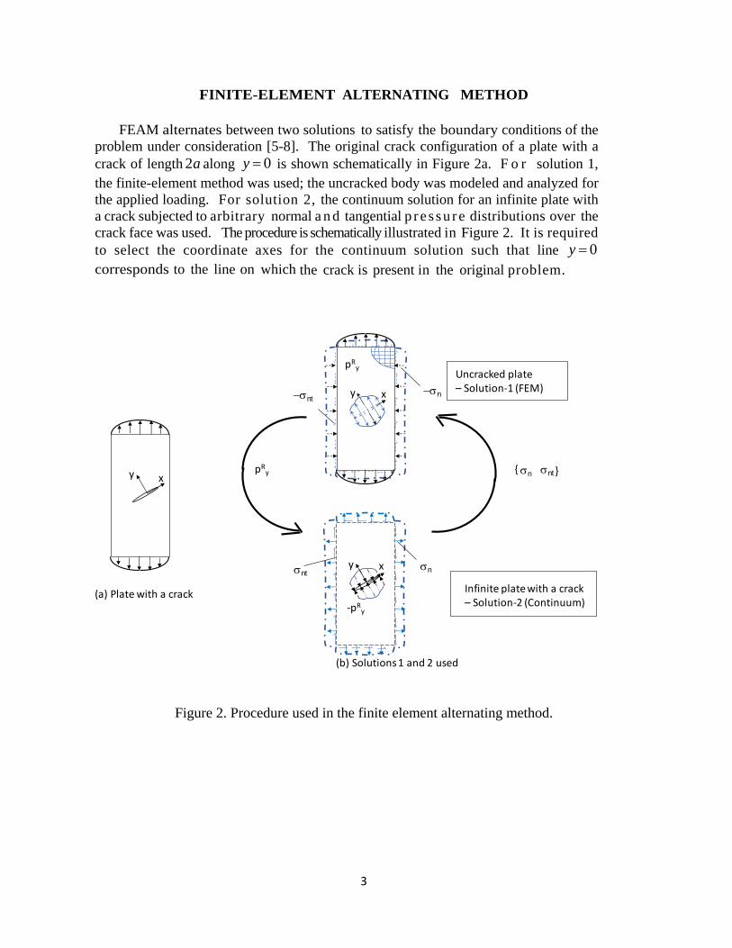
FINITE-ELEMENT ALTERNATING METHOD

FEAM alternates between two solutions to satisfy the boundary conditions of the

problem under consideration [5-8]. The original crack configuration of a plate with a crack of length 2a along 0y is shown schematically in Figure 2a. F o r solution 1, the finite-element method was used; the uncracked body was modeled and analyzed for the applied loading. For solution 2, the continuum solution for an infinite plate with a crack subjected to arbitrary normal a n d tangential p r e s su r e distributions over the crack face was used. The procedure is schematically illustrated in Figure 2. It is required to select the coordinate axes for the continuum solution such that line 0y corresponds to the line on which the crack is present in the original problem.

Figure 2. Procedure used in the finite element alternating method.

pRy ntn }{

(a) Plate with a crack

Uncracked plate – Solution‐1 (FEM)

Infinite plate with a crack – Solution‐2 (Continuum)

(b) Solutions 1 and 2 used

xynt

‐pRy

n

xy nnt

pRy

xy

4

The following steps are involved in the FEAM:

Step 1. Construct a finite element model without actually modeling the crack in the structure.

Step 2. Finite element analysis is performed to obtain the finite element stresses everywhere in the plate for the external applied loading and boundary conditions. Because of the mixed-mode configurations considered here, both the normal and tangential tractions will be present along the 0y line.

Step 3. If either normal or tangential or both tractions are not negligible, go to Step 4. If

both the normal and tangential tractions are negligibly small (i.e. smaller than a prescribed tolerance level), stop the algorithm and calculate the sum of the stress-intensity factors computed so far from the continuum solution.

Step 4. To free the tractions on the crack faces, normal tractions ( )Yp and tangential

tractions ( )Xp along the 0y line computed in Step 3 must be erased. To erase these

tractions, the negative of crack-face normal tractions ( . . )RY Yi e p p and crack face

tangential tractions ( . . )RX Xi e p p are applied to the analytical solution. The tractions

RYp and R

Xp can be expressed in polynomial form for a Nth order polynomial as

0

0

nNTR

Y nn

nNTR

X nn

xp A P A

a

xp B P B

a

(1)

where

2

1, , , ,N

T x x xP

a a a

(2)

and

x is the distance measured from the center of the crack.

The coefficients A and B in eq. (1) are calculated using a least square procedure

[5] as

5

1

1

A H D

B H C

(3)

where

1

1

1

( )

( )

C

j

C

j

C

j

NT

j l

NRY

j l

NRX

j l

H P P dx

D P p x dx

C P p x dx

(4)

In Equation 4, CN is the number of elements over the crack and jl is the length of the thj

finite-element along the crack line. The integrals in these equations are computed by using Gaussian quadrature because discrete values of ( )R

Yp x and ( )RXp x are available from the finite- element

method for each of the CN elements over the crack line. Step 5. Once the coefficients A and B are determined from eq. (3), the stress-intensity

factors for the current r t h iteration a r e c a l c u l a t e d

0

0

Nr rI w nn

n

Nr rII w nn

n

K k A

K k B

( 5 )

where ( )w nk are the stress-intensity factor weights given in Table 1.

Step 6. The crack-face normal RYp and tangential R

Xp tractions obtained in Step

4 create tractions on all the finite element model boundaries of the plate. The stresses at any point on any boundary for each of the polynomial functions can be obtained as

,M A L B (6)

where

6

, , .X Y XY

Table 1. Stress-intensity factor weights for a crack in an infinite plate subjected to

normal ( )Yp and tangential pressure ( )Xp distributions of the form n

x

a

[7].

n w nk

0 1 2 3 4 5 6 7 8

1 1/ 2

1/ 2 3 / 8

3 / 8 5 /16

5 /16 35 /128

35 /128 The positive and negative signs in this table refer to the crack tips at x = ±a, respectively. The negative values are meaningful only in the presence of additional forces, which prevent crack closure.

In Equation (6), the matrices M and L relate the stresses at any point on

the boundary to the unit values of the polynomial normal and tangential pressure distribution over the crack faces, respectively. The matrices [ ]M and [ ]L are obtained using the stress function in the continuum solution due to polynomial pressure distribution over the crack faces [7,8].

Once the stresses on the boundary are obtained, the tractions, XT and YT , in the x-

and y-directions respectively can be calculated us ing

,T q (7)

where

7

, and

0.

0

T

X Y

X y

Y X

T T T

n nq

n n

(8)

In Equation 8, Xn and yn are direction cosines of the normal to the boundary with respect

to x- and y- axis, respectively.

Step 7. To satisfy the traction-free boundary conditions o n the external b o u n d a r i e s , the tractions created due to the residual pressures on the crack tip in Step 6 need to be erased. Therefore, the negative of these transactions are considered as the applied tractions for the finite-element model for the uncracked plate. These tractions can be expressed as nodal forces for each of the elements on the external boundaries as

n tr r rQ G A G B (9)

where

Φ

Φ (10)

In equation (10), ml refers to the thm element under consideration; [Φ are the element shape

functions; and q is the direction cosine matrix defined in equation (8). The matrices M

and L are defined in equation (6).

The nodal forces are assembled to form a global load vector and treated as applied forces on the uncracked body. This is the start of the next iteration. These iterations are continued until the crack face tractions in Step 3 are negligibly small compared to the first iteration. In the converged solution, the mode I and mode II stress-intensity factors are simply the sum of the stress-intensity factors from all the iterations.

8

Computational aspects of the FEAM

In the finite element part of the method, 8-noded isoprametric quadratic elements were used to model the uncracked body. Some computational aspects that make the method efficient are briefly discussed.

Decomposition of the global stiffness matrix: In the FEAM, the uncracked body is analyzed

by the finite element method several times (as many times as the number of iterations required for convergence of stress–intensity factors) with a different load vector obtained from the continuum solution each time. Therefore, the finite element stiffness equations can be written as

0 1 2 0 1 2[ ] , , , , , ,K u u u Q Q Q (12)

where [K] is the assembled stiffness matrix and {ur} is the displacement vector corresponding to the load vector {Q r} for the r th iteration. Equation (12) can be efficiently solved by finding the Cholesky factors of the stiffness matrix [K] soon after the stiffness matrix is assembled. This decomposition needs to be performed only once. Thereafter, the displacements {ur} can be obtained inexpensively because the back substitutions consume far less computing effort than the decomposition of the stiffness matrix. Because of this feature and that the crack length under consideration need not end at an element boundary (see Figure 4 in reference 4), several crack lengths can be analyzed with a single finite element model for the uncracked body in a single run. Boundary Tractions: In step 7 of the method, the nodal forces on each element on all the boundaries are obtained. This computation can be efficiently performed by calculating the [G] matrices in Eq. (10) for all elements on the boundaries before the start of the first iteration. In each iteration, only one matrix multiplication in Eq. (9) is required for each element on the boundaries.

Stress Averaging: In general, stresses computed by the FEM from the elements in the uncracked body along and on either side of the ‘crack line’ will not be equal. The stresses computed at the 2x2 Gaussian points at either side of the ‘crack line’ are extrapolated to the ‘crack line’, and the stresses are averaged (see Figure 3).

9

Figure 3. 2X2 Gaussian points near the crack line used for element stress computation.

Fictitious Pressures: The analytical solution used in the FEAM is based on the embedded crack in an infinite plate. The embedded crack has two crack tips. However, in edge crack problems, only one crack tip exists. Hence to use FEAM for edge crack problems, a fictitious crack is usually assumed with crack tip at x = - a, as illustrated in Figure 4. While for 0 x a the residual pressures are computed from the finite element solution, the residual pressures over the fictitious part of the crack, 0,a x need to be defined. In this paper, four different pressure distributions were used over the fictitious part of the crack. These are shown in Figure 4, ( )I linear extrapolation from x a and 0 to x x a , ( )II constant over 0, ( )IIIdistribution in the region 0a x is mirror image of distribution over 0 x a , and ( )IVdistribution linearly approaching zero at x a . The single edge crack problem is studied with these four fictitious pressure distributions.

Figure 4. Pressure distribution extrapolation for the fictitious part of the edge cracks.

∂ ∂ ∂

∂ ∂ ∂

X X X X X X

X X X X X X

X X X X X X

X X X X X X

X 2X2 Gaussian points

Nodes in the FE model

Crack line

Elements ‘below’ the crack line

Elements ‘above’ the crack line

pR y or pRx

pR y(pR y)0

I

II

III

IV

x

a a

10

Results and Discussion

In this section, the performance of the current FEAM algorithm was evaluated by comparing the results with those available in the literature. First, embedded crack problems were considered. Then edge crack problems, followed by problems with cracks emanating from stress concentrations such as a circular hole were analyzed. As mentioned previously, the FEM part of the method used only idealization of the uncracked body. The uncracked configurations use - 8-node isoprametric elements. In all the problems studied, a value of Young’s modulus,

,E equal to 710 psi and a Poisson ratio of 0.3were used. References 7 and 8 established that the FEAM works equally well with various types of loadings, including tensile, bending and parabolic loadings. Hence, in this paper for all problems studied, only a remote uniform tensile loading S is considered.

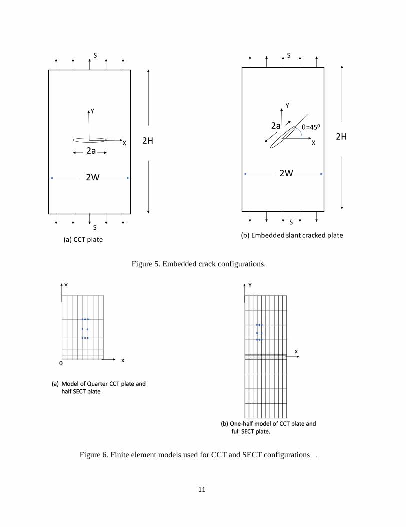
Embedded Crack problems: Figure 5 shows a plate with a straight center cracked (CCT) and a plate with an embedded slant crack oriented at 45 degrees to the x axis. Both configurations were subjected to remote tensile loading. CCT Configuration: Because of the double symmetries of the problem, a quarter model of the uncracked CCT plate can be used. The finite element model shown in Figure 6(a) had 173 nodes and 48 quadratic 8-node elements. Nodes at 0x were prescribed u-displacements equal to zero and nodes at y = 0 were prescribed v-displacements equal to zero. The boundaries on x = W and y = H were made stress free in the algorithm. The CCT specimen was also modeled using the half symmetry in the problem. Figure 6(b) shows a half a symmetry model of the CCT specimen with 405 nodes and 120 elements. For all nodes at line 0x , the u-displacements were prescribed zero. One node at 0x and y H in the finite element model was prescribed 0v . The boundaries on y = H and –H and x = W were made stress free in the algorithm. Table 2 shows the normalized stress-intensity factor, FI, for an (a/W) = 0.5 configuration with these two models for various values of the maximum degree of polynomial, N, used in the algorithm. Also included in the table the number of iterations required to obtain a difference in stress-intensity factor within one percent between two consecutive iterations. Excellent agreement was obtained with reference values from reference 4. This suggests that for CCT configurations, any value of N= 0, 1, 2 or 3 is capable of producing accurate stress-intensity factors with about 5 to 6 iterations.

11

Figure 5. Embedded crack configurations.

Figure 6. Finite element models used for CCT and SECT configurations .

2a2H

2W

(a) CCT plate(b) Embedded slant cracked plate

X

Y

S

S

2a2H

2W

=450

X

Y

S

S

12

Table 2. Normalized stress-intensity factors, FI, for a center cracked (CCT) plate for polynomials used to fit the pressure distributions.

( / 0.5, / 2.5, / ( )I Ia W H W F K S a

Degree of

Polynomial, N Number of Iterations

FEAM

IF

Reference Value (Murakami [4])

IF

Quarter Plate Model

Figure 6(a) 173 Nodes

48 Elements

0 1 2 3 4

5 6 6 6 6

1.184 1.186 1.186 1.188 1.180

1.187

Half Plate Model

Figure 6(b) 405 Nodes

120 Elements

0 1 2 3 4

6 6 7 5 6

1.184 1.186 1.187 1.187 1.186

1.187

Embedded slant crack configuration:

Figure 7 shows the finite element model used for the embedded 45 degree slant crack configuration. The finite element model had 277 nodes and 80 elements. In order to preclude rigid body modes, the u - displacements were set equal (prescribed) to zero at two different nodes and at one of these nodes, v - displacement was also prescribed to be zero. All external boundaries were made stress free in the algorithm. The problem has two crack tips and hence the algorithm computes the stress-intensity factors at both the crack tips. The stress-intensity factors are, as expected, computed to be identical. Table 3 presents the stress-intensity factors for various values of maximum degree of polynomial, N, used in the fit and the number of iterations required. As this is a mixed mode fracture problem, both FI and FII are computed and presented in Table 3. Accurate reference values from reference 4 are included in the table. The stress-intensity factors remain nearly the same as the value of N is increased from 0 to 4 with about 4 iterations. The results in Tables 2 and 3 for embedded crack configuration show that the pressure distributions using constant, linear, or quadratic polynomial FEAM gave accurate stress-intensity factors with about 4 iterations.

13

Figure 7. Finite Element models used for embedded slant crack configuration.

Table 3. Normalized stress-intensity factors, IF and ,IIF for an embedded slant cracked plate

for polynomials used to fit the pressure distributions. ( / 0.5a W , / 2H W 45 ,

/ , / .

Degree of Polynomial, N

Number of Iterations

*FEAM Reference Value (Murakami [4])

IF IIF IF IIF

0 1 2 3 4

5 4 4 4 4

0.607 0.604 0.599 0.599 0.598

0.541 0.539 0.541 0.541 0.541

0.612 0.546

* Full plate modeled with 277 nodes and 80 elements.

14

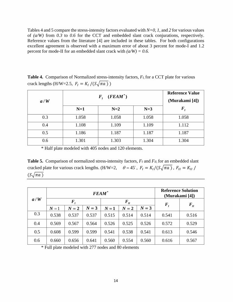
Tables 4 and 5 compare the stress-intensity factors evaluated with N=0, 1, and 2 for various values of (a/W) from 0.3 to 0.6 for the CCT and embedded slant crack conjurations, respectively. Reference values from the literature [4] are included in these tables. For both configurations excellent agreement is observed with a maximum error of about 3 percent for mode-I and 1.2 percent for mode-II for an embedded slant crack with (a/W) = 0.6.

Table 4. Comparison of Normalized stress-intensity factors, FI, for a CCT plate for various

crack lengths (H/W=2.5, /

/a W

*( )IF FEAM Reference Value

(Murakami [4])

IF N=1 N=2 N=3

0.3 1.058 1.058 1.058 1.058

0.4 1.108 1.109 1.109 1.112

0.5 1.186 1.187 1.187 1.187

0.6 1.301 1.303 1.304 1.304

* Half plate modeled with 405 nodes and 120 elements.

Table 5. Comparison of normalized stress-intensity factors, FI and FII, for an embedded slant

cracked plate for various crack lengths. (H/W=2, 45 , / , /

/a W

*FEAM Reference Solution

(Murakami [4])

IF IIF IF IIF

1N 2N 3N 1N 2N 3N 0.3 0.538 0.537 0.537 0.515 0.514 0.514 0.541 0.516

0.4 0.569 0.567 0.564 0.526 0.525 0.526 0.572 0.529

0.5 0.608 0.599 0.599 0.541 0.538 0.541 0.613 0.546

0.6 0.660 0.656 0.641 0.560 0.554 0.560 0.616 0.567

* Full plate modeled with 277 nodes and 80 elements

15

Edge Crack Problems:

Figure 8. Single edge crack (SECT) plate configurations.

Two edge crack configurations are presented in Figure 8. Figure 8(a) shows a zero-degree Single Edge Crack Tension (SECT) and Figure 8(b) shows a 45 degree slant edge crack subjected to remote tensile loading.

Single edge crack: The single edge crack in Figure 8(a) can be analyzed with the two finite element models presented in Figure 6. When using the model in Figure 6(a) one-half of the edge-crack problem is analyzed. As such, the v-displacements at y = 0 were prescribed zero and one node, such as the one at (0, H) was prescribed u = 0. The boundaries on x = 0 and x = W and y = H are made stress free. A fictitious pressure distribution of a constant value (distribution-II) in Figure 4 is used in the algorithm.

The normalized stress-intensity factors obtained with various values of N are presented in Table 6 for a crack length of (a/W) = 0.5. Compared to the embedded cracks, this edge crack problem needs a higher order polynomial distribution to yield accurate results. Also, the stress-intensity factors do not show monotonic convergence. For a value of N=6 the FEAM gave a value which is about 1 percent of the accurate value from the literature. All other results from N=2 to 5 had stress-intensity factors that are less accurate than that with N = 6.

(a) Single edge cracked (SECT) plate (b) Slant edge cracked plate

2H

W

a

S

S

xY

2H

W

=450

S

S

x

Y

16

Table 6. Normalized stress-intensity factors, FI, for a single edge cracked plate for polynomials

used to fit the pressure distributions. (a/W=0.5, H/W=2.5, /

Degrees of Polynomial, N


*FEAM

IF


IF

2 3 4 5 6

24 20 20 19 19

3.075 2.934 3.155

2.913 2.862

2.827

* Half plate modeled with 173 nodes and 48 elements.

Next, the same single edge crack problem was analyzed by modeling the entire plate. The finite element model presented in Figure 6(b) was used. The displacement u = 0 was prescribed zero at nodes at (0, -H) and (0, H) and v = 0 was prescribed at the node (W, -H). These boundary conditions restrain all rigid body modes. The boundaries on x=0, x=W and y= H, y=-H were made stress free. Table 7 presents the normalized stress-intensity factors obtained for a crack length of (a/W) = 0.5 for various assumed pressure distributions, I-IV, shown in Figure 4, and for values of N ranging from 4 to 6 for each of these distributions. Pressure distributions I and II were used in references 5 and 6 for corner cracks in 3D solids, and in reference 7 and 8 for edge cracks in plates. As mentioned previously, edge cracks have only one crack tip and the FEAM is based on a continuum solution of a crack in an infinite plate (and hence with two crack tips). As such, when dealing with edge cracks, one needs to deal with a pressure distribution in the range 0. The solution for the stress-intensity factors should be independent of any choice of the pressure distributions. In that context, the distributions III and IV shown in Figure 4 were developed. Distribution - III was assumed to be symmetric and the distribution on 0

is repeated on 0.Distribution- IV was a linear distribution from x = 0 with a zero value at x = -a. The results in Table 7 show that distributions I and II have nearly the same accuracy. Distribution III, because of its symmetry, does not allow odd powers in the distributions and hence gave exactly same value for N=4 and N=5. Distribution – IV was an extreme case and yet yielded results with only a 4 percent error with N=6. The extrapolated linear distribution (Distribution-I) and constant distribution (Distribution –II) are within 3 percent of the reference values. Therefore, for all edge crack problems, a simple constant pressure distribution with 6N is recommended.

17

Table 7. Comparison of normalized stress-intensity factors, FI, for a single edge cracked plate

for various fictitious pressure distributions. (a/W=0.5, H/W=2.5,

Fictitious Pressure

Distributions (Figure 4)

Maximum Degree of

Polynomial, N


*FEAM

IF

Reference Value

(Murakami [4])

IF

I 4 5 6

17 16 16

3.095 2.915 2.895

2.827

II 4 5 6

21 19 19

3.221 2.949 2.914

III 4 5 6

25 25 25

2,849 2.849 2.742

IV 4 5 6

25 23 24

3.483 3.020 2.951


Table 8 presents the normalized stress–intensity factors for various crack lengths, (a/W) = 0.3 to 0.6, for an edge cracked plate. The results were compared with accurate values from reference 4. Very good agreement was observed, except for the long edge crack at (a/W) = 0.6. A finer mesh is probably needed to obtain better accuracy. As seen in Table 8, the number of iterations needed to obtain a converged solution increases with the crack length. It can be concluded that the single edge crack problem requires more iterations to obtain a solution compared to the embedded crack problems.

Table 8. Comparison of Normalized stress-intensity factors, FI, for a SECT plate for various

crack lengths (H/W=2.5, N=6, / ; Constant pressure distribution was used.

/a W Number

of Iterations

*FEAM

IF


IF

0.3 0.4 0.5 0.6

9 12 19 15

1.705 2.132 2.914 4.349

1.655 2.108 2.827 4.043


18

Slant edge crack (): The next problem considered was a slant edge crack with 45

and remote tensile loading. A crack length (a/W) = 0.5 was considered. The finite element model used is presented in Figure 9. The displacement u = 0 was prescribed at nodes at (0, -H1) and (0, H2) and v = 0 is prescribed at the node (W, -H1). These boundary conditions restrain all rigid body modes. All external boundaries were made stress free. A constant pressure distribution (distribution-II) was used. Table 9 presents the normalized stress-intensity factors for various values of N ranging from 2 to 6. Accurate values from Reference 4 were included for comparison. Accurate values are obtained with N = 5 and 6 for both mode-I and mode-II values. Table 9. Normalized stress-intensity factors, FI and FII, for a slant edge cracked plate with (a/W) = 0.5 for polynomials used to fit the pressure distributions. (H1/W = 1, H2/W = 1.5,

450, / , / ); Constant pressure Distribution II

Degree of Polynomial N

*FEAM Figure 6(b)


IF IIF IF IIF

2 3 4 5 6

1.156 1.207 1.138 1.193 1.190

0.609 0.586 0.603 0.606 0.594

1.191 0.600


19

Figure 9. Finite elements models used for embedded slant crack configuration.

Table 10 presents the normalized stress–intensity factors for various crack lengths,( / ) 0.3 0.6a w to , for the slant edge cracked plate. The results were compared with the

reference values from reference 4. A value of 6N was used. Very good agreement (about one percent deviation) was observed for all mode I stress-intensity factors. The mode II values were less accurate with a deviation of about 5 percent.

The single edge crack (SECT) problem with a crack at 0 was a more difficult problem compared to slant edge crack with 45 . For larger crack lengths, large bending was observed in the SECT plate. The 8-node quadratic elements were not well suited for pure bending problems. Also, when the crack is straight ( 0 ) on the axis of symmetry, the shear stresses

xy should be zero. The finite element solution of the full plate cannot produce zero shear stresses;

20

the solution computes small (but non-zero) stresses in comparison to the normal stresses y . To

avoid the spurious tractions on the external boundaries, due to these small shear stresses, the shear stresses computed from the top and bottom elements were averaged. This modification works well for small crack lengths, but as crack length becomes larger, the errors increase and need to be mitigated by more iterations, as evidenced in Table 7. Notice that this situation does not occur for a slant edge crack at 45 from Table 8. This is because the shear stresses along the crack are non-zero and are of comparable value to the normal stresses.

Table 10. Comparison of normalized stress-intensity factors, FI and FII, for a slant edge cracked

plate for various crack lengths. (H1/W = 1, H2/W = 1.5, 450, / , /

; Pressure distribution is constant (II), N=5)

/a W *FEAM


IF IIF IF IIF

0.3 0.4 0.5 0.6

0.877 1.017 1.193 1,471

0.477 0.532 0.606 0.709

0.879 1.010 1.191 1.436

0.450 0.505 0.574 0.674


Edge Crack emanating from a circular hole:

An edge crack emanating from a circular hole with radius R in an infinite plate and loaded with remote uniform stress is shown in Figure. 10. The reference solution [4] available for this problem is for an infinite plate. A plate with / 1.0H W and / 24W R was selected to represent the configuration. The crack inclination angle was selected as 30 degrees. The finite element model for the uncracked plate is shown in Figure 11. The model consists of 1860 nodes and 590 8-node elements. Since the FEM model is for an infinite plate, the traction created by the continuum solution vanishes at infinity. Hence, there was no need to erase the tractions from the continuum solution on the outer boundaries. The tractions were erased only at the hole boundary. The crack length / 0.5c R was considered. Please note that the distance c is the projected length of the crack along the x axis (see Figure 10).

21

The stress intensity factors obtained from the FEAM analysis and from reference solution are presented in Table 11 for various values of N . For polynomial values 2 to 5, the Mode I stress intensity factors were predicted within two percent and the Mode II stress intensity factors are predicted within one percent from the reference solution.

Figure 10. Slant edge crack from a circular hole in a plate configuration.

Figure 11. Finite elements model used for slant edge crack from circular hole in a plate.

00

2H

2W

S

S

R

x

y

a

c

22

Table 11. Comparison of normalized stress-intensity factors, FI and FII, for a slant edge crack

from a circular hole plate. (H/W = 1, 24W R 300, / , /

/c R Maximum Degree of

Polynomial, N

*FEAM Reference Solution

(Murakami (4)]

IF IIF IF IIF

0.5

2 3 4 5 6

1.544 1.447 1.482 1.521 1.560

0.512 0.493 0.511 0.508 0.545

1.519 0.506


Concluding Remarks

The finite element alternating method (FEAM) was presented to analyze two-dimensional fracture problems. The FEAM alternates between an analytical solution and a finite element solution to satisfy the boundary conditions for a specific fracture problem. The analytical solution for arbitrary normal and tangential pressure distributions on the faces of the crack in an infinite plate was used as the fundamental solution. In the finite element part, the uncracked plate was modeled and analyzed subjected to various loadings. Details of the algorithm and its computational and numerical implementations have been discussed.

In this paper, the accuracy of the stress-intensity factors obtained by the use of FEAM with various pressure distributions have been studied. The FEAM was applied to various embedded and edge cracked plate problems. The study showed that for embedded crack problems, simple constant, linear, or quadratic polynomial distributions, (polynomial of order N=0, 1, or 2), produced accurate stress-intensity factors. About four to five iterations were necessary to obtain accurate stress-intensity factors. For edge crack problems, higher order polynomial distributions (N=5 or 6) were needed to obtain accurate stress-intensity factors. As expected, the edge crack configurations needed more iterations to obtain accurate values compared to the embedded crack problems. One reason for needing the higher order distributions was probably due to extensive bending that was seen in the edge crack problems. Furthermore, the accuracy of the mode-I stress-intensity factors was better than the mode-II values.

The FEAM method gave accurate stress-intensity factors for several embedded and edge crack problems. The FEAM algorithm can be used to evaluate stress-intensity factors of complex crack problems and to develop crack length vs stress-intensity factor curves.

23

References:

1. Tada, H., Paris, P. C., and Irwin, G. R., The Stress Analysis of Cracks Handbook. Del Research Corporation, Hellertown, Pennsylvania (1973).

2. Rooke, D. P. and Cartwright D.J. Compendium of Stress Intensity Factors. The Hillingdon Press, Uxbridge, Middlesex (1976).

3. Sih, G. C., Handbook of Stress Intensity Factors, Vol. 1 and 2. Lehigh University, Bethlehem, Pennsylvania (1973).

4. Murrakami, Y., et. al., Stress Intensity Factors Handbook, Vol. 1 and 2., Pergamon Press, Oxford (1987).

5. Nishioka, T. and Atluri, S. N., “Analytical Solutions for Embedded Elliptical Cracks and Finite Element Alternating Method for Elliptical Surface Cracks Subjected to Arbitrary loading,”. Engineering Fracture Mechanics, 17, 247-268 (1983).

6. Nishioka, T. and Atluri, S. N., “An Alternating Method for Analysis of Surface Flawed Aircraft Structural Components,” .AIAA Journal, 21, 749-757 (1983).

7. Raju, I. S., and Fichter, W. B., “A Finite Element Alternating Method for Two-Dimensional Mode I Crack Configurations,” Engineering Fracture Mechanics, 33, 525-540 (1989).

8. Krishnamurthy, T. and Raju, I. S., “A Finite-Element Alternating Method for Two-Dimensional Mixed-Mode Crack Configurations,” Engineering Fracture Mechanics, 36, 297-311 (1990).

use of simple continuum solutions in finite element ... · use of simple continuum solutions in...

Documents