use of the package nlstools to help the t and assess the
TRANSCRIPT

Use of the package nlstools to help the fit and
assess the quality of fit of a gaussian nonlinear
model
Marie Laure Delignette-Muller and Florent Baty
December 5, 2012
The package nlstools provides several tools that help to fit of a gaussiannonlinear model [1] using the fonction nls and to assess its quality of fit.
y = f(θ, x) + ε, ε ∼ N (0, σ)
The aim of this document is to provide examples showing how to use thesetools that help to fit a model to data using the fonction nls, to check thevalidity of the assumptions of the model, to assess its quality of fit, to evaluatethe precision of parameters estimates by use of confidence intervals or regions, ...For details, see the documentation of each function, using the R help command(e.g. ?nlsResiduals). Do not forget to load the library using the functionlibrary before testing the following examples.
> library(nlstools)
Contents
1 Help to fit a model 21.1 Help to define starting values for parameters . . . . . . . . . . . 21.2 Fit and plot of fit . . . . . . . . . . . . . . . . . . . . . . . . . . . 4
2 Analysis of residuals 72.1 Graphics of residuals . . . . . . . . . . . . . . . . . . . . . . . . . 72.2 Residuals tests . . . . . . . . . . . . . . . . . . . . . . . . . . . . 8
3 Confidence region 93.1 Residual sum of squares contours or likelihood contours . . . . . 93.2 Projections of the 95 percent Beale’s confidence region . . . . . . 103.3 Comparison of both representations of the confidence region . . . 13
4 Resampling 144.1 Jackknife . . . . . . . . . . . . . . . . . . . . . . . . . . . . . . . 144.2 Bootstrap . . . . . . . . . . . . . . . . . . . . . . . . . . . . . . . 15
1

1 Help to fit a model
1.1 Help to define starting values for parameters
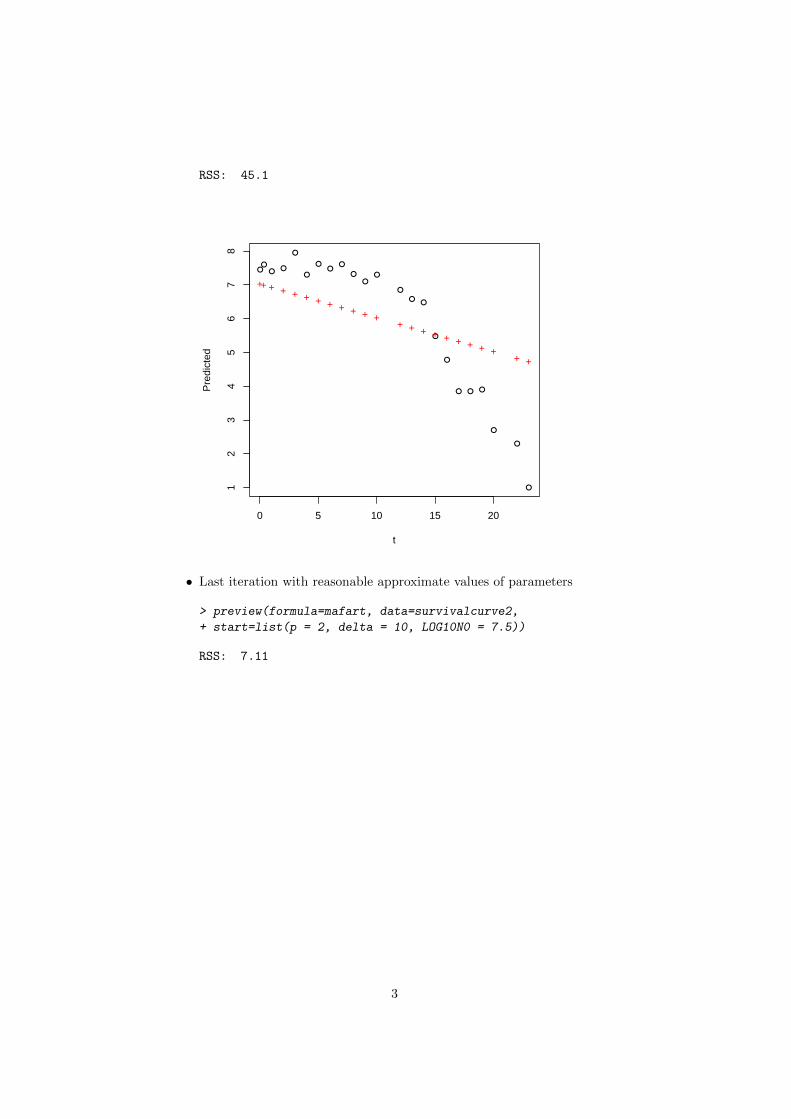
To fit a nonlinear model, it is necessary to specify starting estimates for param-eters. The function preview may be used to facilitate the choice of these values.It provides a superimposed plot of observed (black circles) and predicted (redcrosses) values of the dependent variable versus one of the independent variableswith the model evaluated at specified values of the parameters. The residualsum-of-squares (RSS) give an indication of the distance between observed andpredicted values (the lower, the better). It is then easy to use it repeatedlyto reach a good approximation of the starting estimates as in the followingexample. This example uses a dataset and a model available in the packagenlstools.
• First iteration with arbitrary values of parameters
> data(survivalcurve2)
> preview(formula=mafart, data=survivalcurve2,
+ start=list(p = 1, delta = 1, LOG10N0 = 7))
RSS: 2780
●● ● ●●
●● ● ● ● ● ●
● ● ●
●●
● ● ●
●●
●
0 5 10 15 20
−15
−10
−5
05
t
Pre
dict
ed
+++
++
++
++
++
+
++
++
++
++
+
++
• Second iteration with adjusted values of parameters
> preview(formula=mafart, data=survivalcurve2,
+ start=list(p = 1, delta = 10, LOG10N0 = 7))
2
RSS: 45.1
●●
● ●
●
●
●●
●
●●
●
●
●●
●
●
● ● ●
●
●
●
0 5 10 15 20
12
34
56
78
t
Pre
dict
ed
++ + + + + + + + + + ++ + + + + + + + +
+ +
• Last iteration with reasonable approximate values of parameters
> preview(formula=mafart, data=survivalcurve2,
+ start=list(p = 2, delta = 10, LOG10N0 = 7.5))
RSS: 7.11
3

●●
● ●
●
●
●●
●
●●
●
●
●●
●
●
● ● ●
●
●
●
0 5 10 15 20
12
34
56
78
t
Pre
dict
ed
++ + + + + + + + + ++
++
++
++
++
+
+
+
1.2 Fit and plot of fit
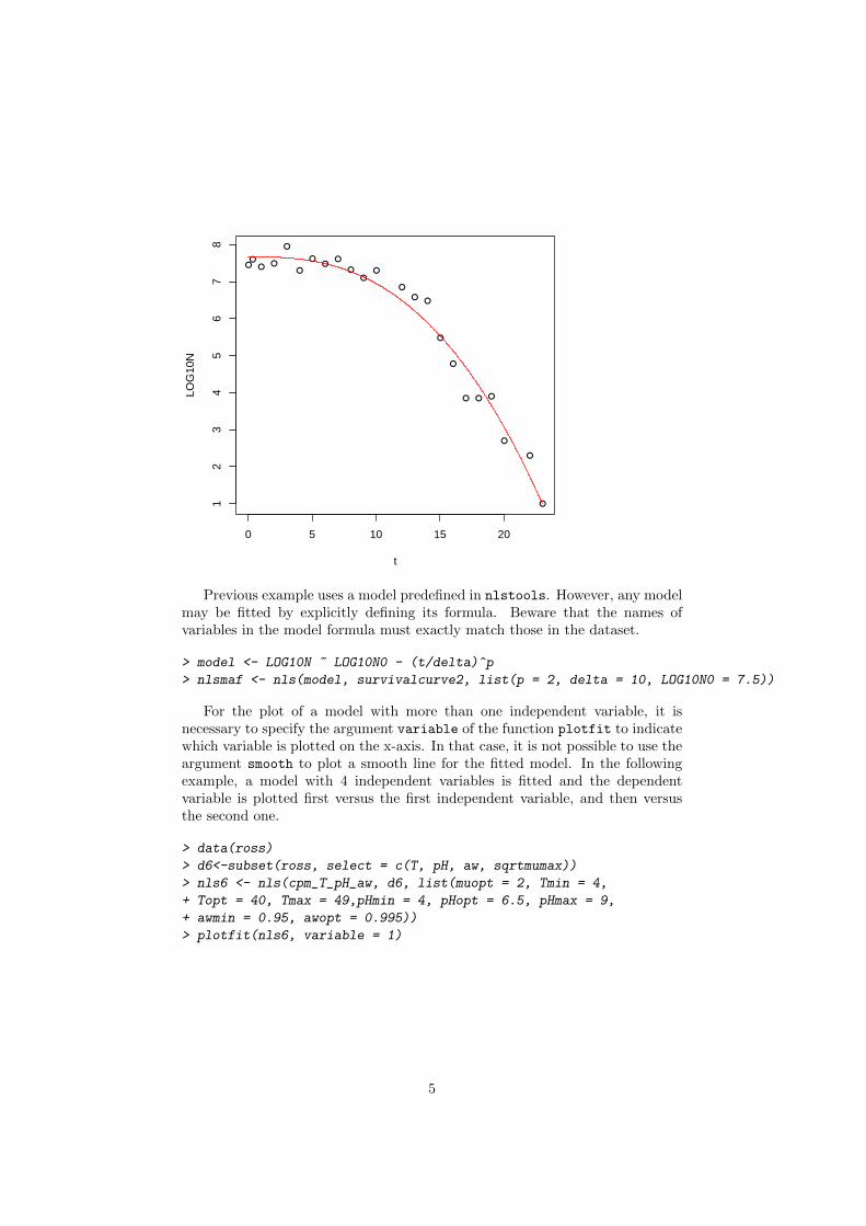
When reasonable starting estimates are available for parameters, the model maybe fitted using the function nls, and the fitted model may be plotted togetherwith the observed data points using the function plotfit. Its argument smoothenables to draw a smooth line for the fitted model.
> nlsmaf <- nls(mafart, survivalcurve2, list(p = 2, delta = 10, LOG10N0 = 7.5))
> plotfit(nlsmaf,smooth=TRUE)
4
●●
● ●
●
●
●●
●
●●
●
●
●●
●
●
● ● ●
●
●
●
0 5 10 15 20
12
34
56
78
t
LOG
10N
Previous example uses a model predefined in nlstools. However, any modelmay be fitted by explicitly defining its formula. Beware that the names ofvariables in the model formula must exactly match those in the dataset.
> model <- LOG10N ~ LOG10N0 - (t/delta)^p
> nlsmaf <- nls(model, survivalcurve2, list(p = 2, delta = 10, LOG10N0 = 7.5))
For the plot of a model with more than one independent variable, it isnecessary to specify the argument variable of the function plotfit to indicatewhich variable is plotted on the x-axis. In that case, it is not possible to use theargument smooth to plot a smooth line for the fitted model. In the followingexample, a model with 4 independent variables is fitted and the dependentvariable is plotted first versus the first independent variable, and then versusthe second one.
> data(ross)
> d6<-subset(ross, select = c(T, pH, aw, sqrtmumax))
> nls6 <- nls(cpm_T_pH_aw, d6, list(muopt = 2, Tmin = 4,
+ Topt = 40, Tmax = 49,pHmin = 4, pHopt = 6.5, pHmax = 9,
+ awmin = 0.95, awopt = 0.995))
> plotfit(nls6, variable = 1)
5

●
●●
●●
●●
●
●
●
●
●
●
●
●
●●
●
●●
●
●●
●
●
●
●
●
●
●●
●●
●
●
●
●
●
●
●
●
●
●
●
●
●
●
●
●
●
●
●
●●
●
●●●
●
●●
●
●
●
●
●●
●●●●●
●
●
●●
●●●●
●
●
●●
●●
●
●
●●
●
●
●
●
●
●
●
●
●
●
●
●
●
●
●●●●●●
●
●
●
●●
●●
●●
●
●●
●●
●
●
●●
●●
●
●
●
●
●
●
●●●
●●●
●
●
●
●
●
●
●
●●
●●●
●
● ● ●
● ● ● ● ●
●
●
●
●
●
●●
●
●
●
●
●
●
●
●
●●●
●
●
●
●
●
●
●
●
●●●
●●
●
●
●
●
●
●
●●●
●●
●
●
●
●
●
●
●●●
●●
●
●
●
●
●
●
●
●
●●
●●
●
●
●
●
●
●
●
●
10 20 30 40
0.2
0.4
0.6
0.8
1.0
1.2
T
sqrt
mum
ax
+
+
+++
+
++
++
+++
++
++
+
+
+
+
+
+++++
++
+
+
+
+++++
+
++++++
++++++
+
+
+
++++
++
+++
+
+
++
+++++++
+
+++++
+
++++++++
++++
++++
+
+
++
+
+++++++++
++
+
++++++++++++++++++
++
+
+++++++++
++
+
+
++++++++
++
++ + + +
+
+
+
+++++++++++
++++++++++++
++++++++++++
+++++++++++
++++++++++++
+
++++++++++++
> plotfit(nls6, variable = 2)
●
●●
● ●
●●
●
●
●
●
●
●
●
●
●●
●
●●
●
●●
●
●
●
●
●
●
●●
●●
●
●
●
●
●
●
●
●
●
●
●
●
●
●
●
●
●
●
●
●●
●
●●●
●
●●
●
●
●
●
●●
●●● ●
●
●
●
● ●
● ● ●●
●
●
● ●
●●
●
●
●●
●
●
●
●
●
●
●
●
●
●
●
●
●
●
●●●●●●
●
●
●
●●
●●
●●
●
●●
●●
●
●
●●
●●
●
●
●
●
●
●
●●●
●●●
●
●
●
●
●
●
●
●●
●●●
●
●●●
●●●●●
●
●
●
●
●
●●
●
●
●
●
●
●
●
●
●●●
●
●
●
●
●
●
●
●
●●●
●●
●
●
●
●
●
●
●●●
●●
●
●
●
●
●
●
●●●
●●
●
●
●
●
●
●
●
●
●●
●●
●
●
●
●
●
●
●
●
4 5 6 7 8
0.2
0.4
0.6
0.8
1.0
1.2
pH
sqrt
mum
ax
+
+
+ + +
+
++
++
++ +
++
++
+
+
+
+
+
++ +++
++
+
+
+
++ +
+ +
+
++
++
++
+++
++
+
+
+
+
++
+ +
++
+++
+
+
++
++
++
+++
+
++
+ + +
+
+++ +
+++ +
++++
+++
+
+
+
+++
++++++++++++
+++++++++++++++++++++
++++++++++++
+
++++++++++++++++
+
+
+++++++++++
++++++++++++
++++++++++++
+++++++++++
++++++++++++
+
++++++++++++
6
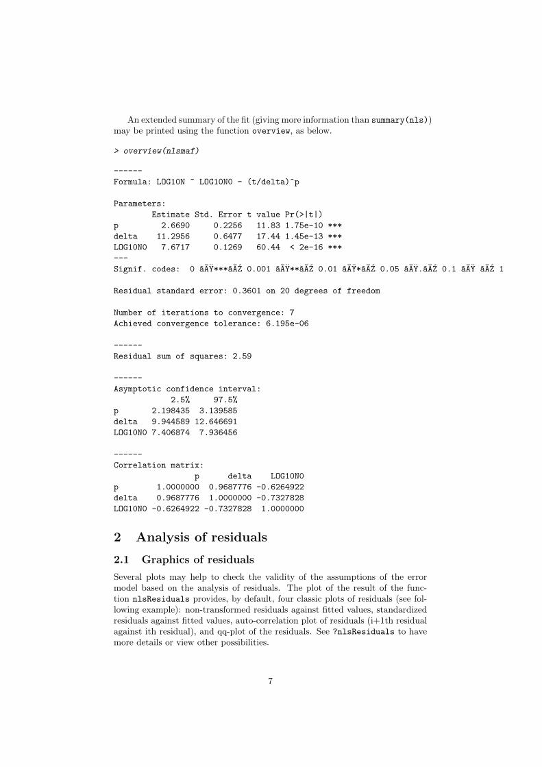
An extended summary of the fit (giving more information than summary(nls))may be printed using the function overview, as below.
> overview(nlsmaf)
------
Formula: LOG10N ~ LOG10N0 - (t/delta)^p
Parameters:
Estimate Std. Error t value Pr(>|t|)
p 2.6690 0.2256 11.83 1.75e-10 ***
delta 11.2956 0.6477 17.44 1.45e-13 ***
LOG10N0 7.6717 0.1269 60.44 < 2e-16 ***
---
Signif. codes: 0 aAY***aAZ 0.001 aAY**aAZ 0.01 aAY*aAZ 0.05 aAY.aAZ 0.1 aAY aAZ 1
Residual standard error: 0.3601 on 20 degrees of freedom
Number of iterations to convergence: 7
Achieved convergence tolerance: 6.195e-06
------
Residual sum of squares: 2.59
------
Asymptotic confidence interval:
2.5% 97.5%
p 2.198435 3.139585
delta 9.944589 12.646691
LOG10N0 7.406874 7.936456
------
Correlation matrix:
p delta LOG10N0
p 1.0000000 0.9687776 -0.6264922
delta 0.9687776 1.0000000 -0.7327828
LOG10N0 -0.6264922 -0.7327828 1.0000000
2 Analysis of residuals
2.1 Graphics of residuals
Several plots may help to check the validity of the assumptions of the errormodel based on the analysis of residuals. The plot of the result of the func-tion nlsResiduals provides, by default, four classic plots of residuals (see fol-lowing example): non-transformed residuals against fitted values, standardizedresiduals against fitted values, auto-correlation plot of residuals (i+1th residualagainst ith residual), and qq-plot of the residuals. See ?nlsResiduals to havemore details or view other possibilities.
7

> resmaf<-nlsResiduals(nlsmaf)
> plot(resmaf)
●
●
●●
●
●
●●
●
●●
●●●
●
●
●
●
●
●
●
●
●
1 2 3 4 5 6 7
−0.
8−
0.2
0.2
0.6
Residuals
Fitted values
Res
idua
ls
●
●
●●
●
●
●●
●
●●
●●●
●
●
●
●
●
●
●
●
●
1 2 3 4 5 6 7
−2
−1
01
2
Standardized Residuals
Fitted values
Sta
ndar
dize
d re
sidu
als
●
●●
●
●
●●
●
●●
● ●●
●
●
●
●
●
●
●
●
●
−0.8 −0.4 0.0 0.4
−0.
8−
0.2
0.2
0.6
Autocorrelation
Residuals i
Res
idua
ls i+
1
●
●
●●
●
●
●●
●
●●
●● ●
●
●
●
●
●
●
●
●
●
−2 −1 0 1 2
−2
−1
01
Normal Q−Q Plot of Standardized Residuals
Theoretical Quantiles
Sam
ple
Qua
ntile
s
2.2 Residuals tests
The normality of residuals may be tested by the Shapiro-Wilk test and theirindependence by the runs test using the function test.nlsResiduals as below.
> test.nlsResiduals(resmaf)
------
Shapiro-Wilk normality test
data: stdres
W = 0.968, p-value = 0.6407
------
Runs Test
data: as.factor(run)
Standard Normal = -0.2045, p-value = 0.8379
alternative hypothesis: two.sided
8

3 Confidence region
The package nltools provides two different methods for the representation of1− α confidence region for model parameters as defined by Beale [1, 2]:
SCE(θ) < SCEmin
[1 +
p
n− pF1−α(p, n− p)
]The function nlsContourRSS provides sections of that confidence region on eachplane defined by two parameters, while the function nlsConfRegions providesprojections of that region on the same planes.
3.1 Residual sum of squares contours or likelihood con-tours
The function nlsContourRSS enables to plot the Residual Sum of Squares (RSS)contours which also correspond to the likelihood contours for a Gaussian model.One of these contours, plotted in red, corresponds to the section of the 95 percentBeale’s confidence region in each plane of two parameters. The argument nlevcorresponds to the number of contours to be plotted, in addition to the red one.
> contmaf <- nlsContourRSS(nlsmaf)
> plot(contmaf, col=FALSE, nlev=10)
p
delta
2.0 2.5 3.0 3.5
910
1112
1314
p
LOG
10N
0
2.0 2.5 3.0 3.5
7.2
7.4
7.6
7.8
8.0
8.2
delta
LOG
10N
0
9 10 11 12 13 14
7.2
7.4
7.6
7.8
8.0
8.2
9
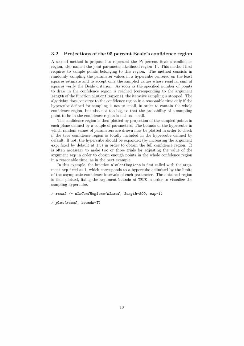
3.2 Projections of the 95 percent Beale’s confidence region
A second method is proposed to represent the 95 percent Beale’s confidenceregion, also named the joint parameter likelihood region [1]. This method firstrequires to sample points belonging to this region. The method consists inrandomly sampling the parameter values in a hypercube centered on the leastsquares estimate and to accept only the sampled values whose residual sum ofsquares verify the Beale criterion. As soon as the specified number of pointsto draw in the confidence region is reached (corresponding to the argumentlength of the function nlsConfRegions), the iterative sampling is stopped. Thealgorithm does converge to the confidence region in a reasonable time only if thehypercube defined for sampling is not to small, in order to contain the wholeconfidence region, but also not too big, so that the probability of a samplingpoint to be in the confidence region is not too small.
The confidence region is then plotted by projection of the sampled points ineach plane defined by a couple of parameters. The bounds of the hypercube inwhich random values of parameters are drawn may be plotted in order to checkif the true confidence region is totally included in the hypercube defined bydefault. If not, the hypercube should be expanded (by increasing the argumentexp, fixed by default at 1.5) in order to obtain the full confidence region. Itis often necessary to make two or three trials for adjusting the value of theargument exp in order to obtain enough points in the whole confidence regionin a reasonable time, as in the next example.
In this example, the function nlsConfRegions is first called with the argu-ment exp fixed at 1, which corresponds to a hypercube delimited by the limitsof the asymptotic confidence intervals of each parameter. The obtained regionis then plotted, fixing the argument bounds at TRUE in order to visualize thesampling hypercube.
> rcmaf <- nlsConfRegions(nlsmaf, length=500, exp=1)
> plot(rcmaf, bounds=T)
10

+
+
+
+
+
+
++++
+
+
+
+
+
++ +
+
+
+
+
+
+
+
++
++
+ +
+
+
+
+
++
++
++
++
++
+
+
+
+
++ ++
+
+
+
++
++
+
++
+
+
+
+
+
+
+
+
+
++
+
++
++
+
+
+
+
++
++
+
+
+
+
+
+
+
+
+
+
+
++
+
+
+
++
+
+
+
++
+
+ ++
+
+
+
+
+
+
+
+
+
+
+
+
+
+
+
+
+
+
++
+
+
+
++
++
+
++ +
+
+
+
+
+
+
+
+
+
+
+
+
+
+
++
+
+
+
+
+
+
+
+
+
++
+
+
+
++
+
+
+
+
+
+
+ +
+
+
+
+
+
+
+
+
+
+
++
+
+
+
+
+
++
+
+
+
+
+++
+
+
++
+
+
+
+
+
+
+
+
+
+
+
+
+
+
+
+
++
+
++
+ ++
+
+
+
++
+
+
++
+
+
++
+
+
+
++
+
++ +
++
++
+
+
+
+
+
+
+
+
+
++
+
++
+
+
+
+
+
+
+
+
+
+
+
+
+
+
+
+
+
++
+
+
+
+
+
+
++
+
+
+ ++
++
++++
+ +
+
+
+
+
++
+
+
+ ++
+
++
+
+
++ +
+
+
+
+
+
++
+
+
+
+
+
+
+
+
+++
+
+
+
+
+
+
+
+
+
+
+
++
+
+
+
+++
+
+
+
+
+
+
+
+
+
+
+
+
+ ++
+
+
+
+
+
++
+
+
+
+
++
+
+
+
++
+
+ +++
+
+
++
++
+
+
+
+
+
+
+
+
+
+
+
+
+
+
+
+
++
+
+
+
++
+
+
+
+
++
++
+
+
+
+
+
++
+
+
+
+
+
++
++
+
+++
+
+
+
++
+
+
++
+
+
+++
+
+
+
+
+
++
++
++ +
+
++
+
2.2 2.4 2.6 2.8 3.0
10.0
11.0
12.0
p
delta
+
+ +
+
+ +
++
+
++
+
+
+
++
+
++
+
+
+
+
++
+
++
+
+
+
+
++
+
+++
+
+
+
+
+
+ +
+
++
+
++
+
+
+
+
+
+
+
+
+
+
+ +
+
++
+ +
+
+
+
++
+
+
++
+
+
+
+
++
+
+
+
++
+ ++
+
++
+
+
+
+ +
+ +
+
+
+
+
++
+
+
+
+
+
+
+
++
+
+
+
++
+
+
+
++
+
++
++
+ +
++
+
+
++
++
++
+
+
+
+
+
+
+
+
+
+ +
++
+
+
+
+
+
+
+
+
+
+
+
+
+
+
+
++
+
+
+
+ +
+
+
+
+
+
+
+
+
+
+
+ ++
+
++
+
+
+
+
+
+
+ ++
+
+
+
+
+
+
++
+
+
+++
+
+
++
+
+
+
+
+
++
++
+
+
+
+
+
+ +
+
+
+
+
+
+
+
+
+
+
++
+
+
+
+
+
+
+
++ ++
+ ++
+
+
++
+
+
+
+
+
+
+
+
+
++
+
+
+
+
+
+
+
+
++
+
++
++
+
+++
+
+
+
+
+
+
++
++
+
+
+
++
+
+
++
++
+
+
+
+
+
+ +
++
+
+
+
+
+
++
++
+
++
+
+
+
+
+
+
+
+
+
+
+
++
+
+
+
+
+
+
+
+
+
+
+
+
+
+
+
+++
+
+
+
+
++
++
+
+++
+
+
+
+
+
+
+
+
+
+
+
++
++
+
+
+
+
++
+
+
++ +
+
++
+
+
+
+
+
+
+ ++ +
+ ++
+
+
+
+
++
++
+
+
+
+
++
+
+
+
+
++
+
+
+
+ ++
+
+
+
+ ++
+
+
+
+
+
++
+
+
++
+
+
++
+
+
+ +
++
+
+
+
+
+
++
+
+
++
+
+
++
+
+
++
++
+
+
+
2.2 2.4 2.6 2.8 3.0
7.4
7.5
7.6
7.7
7.8
7.9
p
LOG
10N
0
+
+ +
+
+ +
++
+
++
+
+
+
++
+
++
+
+
+
+
++
+
++
+
+
+
+
++
+
+++
+
+
+
+
+
+ +
+
++
+
++
+
+
+
+
+
+
+
+
+
+
++
+
++
+ +
+
+
+
++
+
+
++
+
+
+
+
++
+
+
+
++
+ ++
+
++
+
+
+
+ +
+ +
+
+
+
+
++
+
+
+
+
+
+
+
++
+
+
+
++
+
+
+
++
+
++
++
+ +
++
+
+
++
++
++
+
+
+
+
+
+
+
+
+
+ +
++
+
+
+
+
+
+
+
+
+
+
+
+
+
+
+
++
+
+
+
+ +
+
+
+
+
+
+
+
+
+
+
+ ++
+
++
+
+
+
+
+
+
+ ++
+
+
+
+
+
+
++
+
+
+ ++
+
+
++
+
+
+
+
+
++
++
+
+
+
+
+
+ +
+
+
+
+
+
+
+
+
+
+
++
+
+
+
+
+
+
+
++ +
+
+++
+
+
++
+
+
+
+
+
+
+
+
+
++
+
+
+
+
+
+
+
+
++
+
++
++
+
+++
+
+
+
+
+
+
++
++
+
+
+
++
+
+
++
++
+
+
+
+
+
+ +
++
+
+
+
+
+
++
++
+
++
+
+
+
+
+
+
+
+
+
+
+
++
+
+
+
+
+
+
+
+
+
+
+
+
+
+
+
+++
+
+
+
+
++
++
+
+++
+
+
+
+
+
+
+
+
+
+
+
++
++
+
+
+
+
++
+
+
++ +
+
++
+
+
+
+
+
+
+++ +
+ ++
+
+
+
+
++
++
+
+
+
+
++
+
+
+
+
++
+
+
+
+++
+
+
+
+ ++
+
+
+
+
+
++
+
+
++
+
+
++
+
+
+ +
++
+
+
+
+
+
++
+
+
++
+
+
++
+
+
++++
+
+
+
10.0 10.5 11.0 11.5 12.0 12.5
7.4
7.5
7.6
7.7
7.8
7.9
delta
LOG
10N
0
Since the whole region does not seem to be included in the sampling hyper-cube, the function nlsConfRegions is recalled with the argument exp fixed at2.
> rcmaf <- nlsConfRegions(nlsmaf, length=500, exp=2)
> plot(rcmaf,bounds=T)
11

+
+
+
+
+
+
++
+
+++
+
+
+
++
+
+
+
+
+
+
+
+
++
+
+
+
+
+
+
+
+
+
+++
+
+
+
+++
+
+
+
++
+
++
+
+
+
+
+
+
+
++
+ ++
+
++
++
+
+
+
+++
+
+
+
++
+
++
+
+
+
+
+
++
+
+
+
++
+
+
++
++
+++
+
++
+
+
++
+
++
+
++ +
+
+
+
+
+
++
++
+
++
+
+
+
+
+
++
+
+
+
+
++
++++
+
++
+
+
++
+
+++
+
+
+
+
+
++
++
+
+
+
++
++
+
++ +
+
+
+
+
+
+
+
+++
+
++
+
++
+
++
+
+
++
+
+
+
+
+
++
+
+ +
+
+
++
+++ +
+
+
+
+
+
+ +
+
+++
+
+
+
++
+
+
+
+
+
+
+
+
++
+
+
++
+
+
++
+
+
+
+
++
++
+
++
+++
+
++
+
+
+
++
+
++
+
++
+
+
++
++
++
+
+
+ ++
+
+
+
++
+++
+
+
+
+
+
+
+
+++
+
+
+ ++
+
+
+++
+
+
+
++
++
++
+
+
+
++++++
+
+
++
+
+
+
++
+
++
+
++
+
+ +
+++
+ ++
+
+ +
+
+
+
+
+
++
+
+
+
+ +
+
+
+
+
+ +
+
++
++
+++
+
+
+
++
+
++
++
+
+
+
+++
+++
+
+
+
+
+
+++
+
+
+
++
+
+
++
+
+
+
+
++
+
+
+
+
+
++
+
+
+
++
+
+
+ +++
+
++
+++
++
++
+
+
++
+
++++ +
+ +
++
+
+
+
++
++
+
+
+
+++
+
+
+
++
++
++
2.0 2.5 3.0 3.5
910
1112
1314
p
delta
++
+ +
++
+++
++
+
++
+ +
+
+
+
+
+
+
++
+
+
+
+
++
++ +
+
+ +
+
++
+
+
+
++ +
+
++
+
+
+
++
+
+
++
+
+
++
+
+
+
++
+
+
+
+
+
+
+
++ +
+
+ ++
+
+
+
+
+
+
+
+
+ +
+
+
++
++
+
+
++
+
++
+
+
+
++
+
+
+
+
+
+
+
+
+
+
+
++
+
+
+
++
+
+
+
++
+
+
++
+
++
+
++
+
++
++
++
+
++
+
++
++
+++
++
+
+
+
+ +
+
++
++
+
+
+
++
+
+
+
+
+
+
+++
+
+++
+
+
++
++
+
+
+
+
+
++
++
+
+
+
+
++
+
+
+
+
+
+
+
+
+
++ +
+
+
+
+
++
+
+
+
+
+
+++
+
+
+
+
++
+
+
++
+
+
+
+
+
+
+
+
++
+
+ + ++
+
+
+
++++
+
+
+
+
+
+ +
+
+
+ +
+
+
+
+
++
++
+
++
+
++ +
+
+
++
++
+
++
+
+
+
+
+ +
+++
+
+
+
+
+
++
+
+
+
++
++
+
+++
+++
+
+
+
++
++
+
+
+
+++
+
+
+
+
+
+
++
++
+
+
++
++
+ ++
++
+
+
+
+
+
+
++
+
++
+ +
+
+
+
+
+
+
+
++
+
+
+
+
+
+ ++
+
++ + +
++
+
+
+
++ +
+
++
++
+
+
+
+
+
+
+
+
+
+
+++
+
+
+
+
+ +
++
++
+
+
+
+
+ +
+
++
++
+
+
+
+
++
++
+
+
++
+ ++
+
+
+
+
+
++++
++
+
++++
+
+
+
+
+
+
+
++++
+
+
++ +
+++
+
2.0 2.5 3.0 3.5
7.2
7.4
7.6
7.8
8.0
8.2
p
LOG
10N
0
++
+ +
++
+++
++
+
++
+ +
+
+
+
+
+
+
++
+
+
+
+
++
++ +
+
+ +
+
++
+
+
+
++ +
+
++
+
+
+
++
+
+
++
+
+
++
+
+
+
++
+
+
+
+
+
+
+
+++
+
+ ++
+
+
+
+
+
+
+
+
+ +
+
+
++
++
+
+
++
+
++
+
+
+
++
+
+
+
+
+
+
+
+
+
+
+
++
+
+
+
++
+
+
+
++
+
+
++
+
++
+
++
+
++
++
++
+
++
+
++
++
+++
++
+
+
+
+ +
+
++
++
+
+
+
++
+
+
+
+
+
+
+++
+
+++
+
+
++
++
+
+
+
+
+
++
++
+
+
+
+
++
+
+
+
+
+
+
+
+
+
++ +
+
+
+
+
++
+
+
+
+
+
++
+
+
+
+
+
++
+
+
++
+
+
+
+
+
+
+
+
++
+
+ +++
+
+
+
++++
+
+
+
+
+
+ +
+
+
+ +
+
+
+
+
++
++
+
++
+
+++
+
+
++
++
+
++
+
+
+
+
+ +
+++
+
+
+
+
+
++
+
+
+
++
++
+
+++
+++
+
+
+
++++
+
+
+
+++
+
+
+
+
+
+
++
++
+
+
++
++
+++
++
+
+
+
+
+
+
++
+
++
++
+
+
+
+
+
+
+
++
+
+
+
+
+
+ ++
+
++ + +
++
+
+
+
+++
+
++
++
+
+
+
+
+
+
+
+
+
+
+++
+
+
+
+
+ +
++
++
+
+
+
+
+ +
+
++
++
+
+
+
+
++
++
+
+
++
+ ++
+
+
+
+
+
++++
++
+
++++
+
+
+
+
+
+
+
++++
+
+
++ +
+++
+
9 10 11 12 13 14
7.2
7.4
7.6
7.8
8.0
8.2
delta
LOG
10N
0
This value of the argument exp seems reasonable. The function nlsCon-
fRegions may be recalled specifying a greater number of points drawn in theregion (argument length), and the region may be plotted without showing thebounds of the hypercube.
> rcmaf <- nlsConfRegions(nlsmaf, length=2000, exp=2)
> plot(rcmaf, bounds=F)
12

+
+
+
++
++
+
+
+
+
++
+++
+
+
+
+
+
+
+
++
++
+
++
+ ++
+
+
+
+
++
+
+
+
+
+
+
+
+
+
+
+
+
+
+
++
+
+
++
+
+
+
++
+
+ +
+
+
+
+
++
+
+
+
+
+
+
+
+
+
+
+
+
+
+
+
+
+
+
+
+
+
+
+
+
+
+
+
+
+
+
++
+
+
+
+
+
++
++
++
+
+
+
+
++
++
++
+
+
+
++
+
+
+
+
+
+
+
+
+
+
+
+
+
++
+
+
+
+
+
+
++ +
+
+
++
+
+
+
+
+++
+
++
+
++
+
+
+
++
+
+
+
+
+
++
+
+
+
+
+
++
+
+
+
+
+
+
+
+
+
+
+
++
++
+
+
++
+
+
++
+
+
+
+
+
++
+
+
+
+
+
++ +
++
+
+
+
+
+
+
+
+
+
+
+
+
+
+
++ +
++
+
+
+
+
+
+
+
++
+
+
+
+
+
+
+++
++
+
+
++
+
+
++
+
+
+
+
+
+
+
+
+
+
+
+
+
+
+
+
+
+
+
+
+
+
+
+
++
+++
+
+
+
+
+
+
+
+
+
+
+
+
+
+
+
+
++
++
+
+
+
++
+
+++
+
+
+
++
+
+
++ +
+
+
+++
+
++
++
+
++
++
++
+
+
+
+
++
+++
++
++
+
++
+
+
+
+
+
+
+
+
+
+
+
+
+ +
++
+
+ +
++
+
+
+
+
++
+
+
+
+
+
+
+
+
+
+
+
++
++
+
+
+
+
+
+
++ +
+
+
+
+
+
+
+
+
+
+
+
+
+
+
+
+
+
+
+
++++
++
+
+
+
+
+
+
+
+
+
+
+
+
++
+
++
++ +
+
+
++ +
+
++
+ +
+
+
+
+
++
++
+
+++
+
+
+
++
+
+
++
+
+
+
+
++
+
+
+
+
+
+
+
+
++
++
+
+
+
+
+
+
+
+
+ +
+
+
++++
++
+
+ +
+
++
+
++
++
+
+
+
+
+
+
+
+
++
++
+
+
+
+
+
+
+
+
+
+
+
+
++
+
+
+
+
+ +
+
+
+
+
+
+
+
++
+++
+
+
+
++
+
+ +
++
+
+
+
+
+
+
+
+
+
+
+
+
+
+
+
+
++
+++
++
+
+
+
++
+
+
+
++
+
+
+
+
+
+
+
+
+
+
+
+
+
+
+
+
++
+
+
+
++
+
+
+
+
+
+
+
+
+ +
+
+
+
+
++
+
++
++
+
+
+
+
+
+
+
+
+
+
+
+ +
++
+
+
+
++
+
+
+
+
++
+
+
+
+
+
+
+
+
+
+
+
++
+
+
+
+
+
++
++
+
+
+
+ +
+
+
++++
++ +
+
+
+
+
+
+
++
++
+ +
+
+
+
++
+ ++
+
+ +
+
+
+
+
+
++
++
+
+
+
+
+
+
+
+
++
+
++
+
+
++
+
+
+
+
+
+ ++
+
+
+
+
+
+
+
+
+
+
+++
+
+
+
+
+
+
+
+
+
+ +
+
+
+
++
+
+
++
+
+
+++
+
+
+
+
++
++
+
+
+
+
+
+
+
++
++
+
+
+
+
+
+
+
+
+
+++
+
+
+
+
+++
+
+
+
+
+
+
+++
+
+
+
+
+
+
+
+
+
+
+
+
+
+
+
+
+
+
++
+
+++
++
+
+
+
+
+
++
++
+
+
+
+
+
+
+
+
+
+
++
+
+
+
++
+
+
++
+
++
+
+
+
+
++
+
+
+
++
+
+
+
+
+
+++
+
+
++
+++
+
+
+++
+
+
+++
+
+
+++
+
+
+
++
+
+
+
+
+
+
+
++
+
+
+
+
+
+
+
+
+
+
+
+
+
+
+
+
+
+
+
+
+
++
++
++
+
+++
+
+
+
+
+
+
++
+
+
++
+
+
+
+
+
+
++
+
+
+
+
++ +
+
+
+
+
+
+
++
+
+
+
+
+++
+
+
+
+
+
+
+
+
+
++
++
+
++
+
++
+
+
+
+
+
+
++
+
+
+
+
++
+
+
+
+
+
+
+
+
+
+
+
+
+
+
+
+
+
+
++
++
+
+
+
+
+
+ +
+
+
+
++
+
+
+
+
+
++
+
+
+
+
+
+++
++
+
+ ++
+
+
+
+ +
+
+
+
++
+
++
+
+++
+
+
+
+
+
+
+
+
+
+
+
+
+
+
+
+
+
+
+
+
+
++
+
+
+
+
+
+
++
+
++
+
+
+ ++
++
+
+++
+
+
++
+
++
+
+
+
+
++
+
+
+
+
++
+
+
+
++
+
+
+
+
+
+
+
+
+
+
+
++
+
+
+
+
+
+
+
+
+++
+
+++
+ ++
+
+
+
++
+
+
+
+
+
+
+
+
+ +
+
++
+
+
++++
+
++
+
+
+
+
++
+
+
+
+
++
+
+
++
+
+
+
+
+
+
+
+
+
+
+
++
+
+
+
++
+
+
+
++
+
+
+
+
++
+
+
++
+
+
+
++
+
+
+
+
++
+
++
+
+
+
+
+
++
+
+
++
+
+
++
+
++
+
+
+++
+
++
++
+
++
+
+
+
+++
+
+
++
+
++
+
+
+
+
+
+
+
+
+
+
++
++
+
+
+
++
+
+
+
+++
+
++
+
++
++
+
+
+
+ +
++
+
+
+
+ +
++
+
+
+
+
+++
+
+
+
+
+
+
+ +
+++++ ++
+
+
+
+
+
+
+
+
+
+
+
+
+
+
+
+
+
++
++
+
+
+
+
+
+
+
+
++
+
+
+
+
+
++
++
+
+
+
+
++
+
++++
++
+
+
+
+
++
+
++
+
+ +
+
+
+
+
++
+
+
+
++
+
+
+
+
+
+
+
+
++
+
+
+
+
++
+
++
+
++
+++
+
+
+
+
+
+
+
+
+
+
+
+
+
+
+
+
+
+
+
+ +
+
+
+
+
+
+
+
+
++
+
+
+
+
+
++
+
+
+
+
+++
+++
+
+
++
++
++
+
+
+
+
+
+
+
+
+
++
+
+
+
+
+
+
+
+
+
++
+
++
+
++
+
+
+
+
+
+
+
++
+
+++
+
+
+
+
+
+
+ +
++
+
+
+ +
+
+
+
++
+++
+
+
+
+
+
++
+
+
+
+++
+
++
+
++ +
+
+
+
++
+
+
+
+
++
++
+
++
+
+
+
+
+
+
+
+ +
+ +
++
++
+
+
++
+
+
+
++
+ ++
+
+
+
++
++
+
+
+
+
+
+
+
+
++
+
+
+
+
++
+
+
+
+
+
+ +
+
+ +
++
+
+
+
++
++
+
++
+
+
+
+
+
+
+
+
+
+
+
+
+
+
+
++
+
+
+
+
+
++
+
+
+
+
++
+
++
+
+
++
+
+
+
+++
+
+ +
++
+
+
+
+
+
+
+
+
+
+
+
+
+
+
++
+ +
+
++ ++
+
+
+
++
+
+
+
+
+
++
+
+
+
++
+
+
++
+
+
+
+
+
+
+
+
+
+
+
++
+
++
++
+
+
+
+
+
+
+
+
+
+
++
++
+
++
+
+
+
+
+++
+
+
+
+
+
+
++
+
++
+++
+
++
+
+
+
+
+ +
+
+
+
++
+
+
+
+
+
+++
++
+
+
+
+
+
+
++
+
+
+
+
+
+
+ ++
2.2 2.4 2.6 2.8 3.0 3.2 3.4
9.5
10.5
11.5
12.5
p
delta
+
+
+
+
+++
+
++
+
+
+
+
++
+
+
+
+
++
+
+
+
++
+
+
+
+
+
+
+
+
+
+
+
+
+
++
+
+
+
+
+
+
+
+
+
++
+
+ +
+
++
++
+
+
+
+
++
++
+
+
+
+
+
+
+
++
+
++ +
+
+
+
+
+
+
+
+
+
+
+ ++
+
+
+
+
+
+
+
+
++
+
+
+
+
+
+
+
+
+
+
++
+
+
++
+
+
+
+
+ +++
++
+
++
+
+
++
+
+
+
+
+
+
+
++
+
+
+
+
+
+
+
+
+
+
+
+
+
++
+++
+
+
+
+
+
+
+
+
+
+
+
++
+
+
+
+
+
++
+
+
++
+
+
+
++
+ +
+
+
+ +
+
++
+
++
+
+
++
++
++
+
++
+ +
+
+
+ ++
+
+
+
++
+
++
+
++
+
+
+
+ +
++
+
++
+
+
+
+
+
+
+
++
+
+
+
+
+
+
+
+
+
+
++
++
++
+
+
+ +
++
+
+
+
+
++
+
+
+ +
+
+
+
++
+
+
+
+
++
+
+
+
+
+
+
+ +
++
+
+
+
+
+
+
+ +
+
+
+
+
+
+
++
+
+
+
+
++
++
+
+
+
+
+
+
+
+
+
++
+
+
+ +
+ +
+
+
+
+
+
++
+
+
+
++
+
+
+
+
+
+
+
+
+
++
+
+
+
+
++
+
+
+
+
++
+
+
+
+
+
+
+
+
+
+
+
+
+
+++
+
+
+
++
+
+
+
++
++
++
+
++ +
+
+
++
++
+
++
++
+
++
+
++ +
+
+++
+
+
+
+
+
+
+
++
+
+
+
+
++
+
+
+
+
+
+
++
+
+
+
+
+
+
+
+
+
+
+
+ +
+
+
+
+
+
+
+
++
+
++
+
+
+
+
+
++
+
++
+++
+
++
+
+
+
+
+
++
++ +
+
+
+
+
++
+
++
+
+ +
+
+
+
+
+
+ +
+
+
+
+
+
+
+
+
+
+
++
+
+
+
+
++
+
+ +
+
+
+
+
+
++
+
++
+
+
+
+
++
+
+
+++
+
+
+
+
+ +
+
++
++
+
+
+
++ +
++
+
+
+
++
+
+
+
+
+
+
+
++
+
++
+
+
++
+
+
+
+
+
+
+
+ +
+
+
+++ ++
+
+
+
++
+
+++
++
+
+
+
+
+
+
+
+
+
++
+
+
++
+
+++
+
+
+ ++
+
+
+
+
+
+
+
+
+
+
++
+
+
++
+
+
+
+
++
+
+
+
+
+
++ +
+
++
+
+
+
+
+
+
+
+
++
+
+
+
++
+
+
++
+
+
+
++
+
+
+
+
+
+
+
+
+
+
++
+ +
+
+
+
+
++
+
+
++
+
+
+++
+
+
++++
+
+
+
+
+
+
+
+
+
+
++
++
+
+
+
+
++
+
+
+
+
++
+
+
+
+
+
+
++
++
++
+
+
++
+
++
+
+
+
+
+
+
+ ++
+
+
+
+
+
+ +
+
+
+
+
+
+
+
+
+
+
+
+
++
+
+
+
+
+
++
+
+
+
++
++
+
+
+
+
+
+
+
+
+
+
++++
+
++
+
+
++
+
+
+++
+
++ +
+
+
+
++
+ +
++
++
+
+
+
+
+
+
+
++
+
+
+
+
+
+
+
+
+
+
+
+
+
+
+
+
++
+
+
+
+
+
+
+
+
++
+
+
+ +
+
+
++
+
+
++
+
+
+
+
+
+
+
+
+++
+
+
++
+
+
+
+
+
+
+
+
+
+
++
+
++
+
+
++
+
+
+
+
+
+
+
+
+
+++
+
+
++
++
+
+
+
+ +
+
++
+
++
+
+
+
++
+
++
+
+
+
+
++
+
+
+
+
+
+
+
+
+
+
+
+
++
+
+
+
+
++
+
+
++
+ +
+
+
+
+
+
+
+
+
+
+
+
+
+
+
+
+ +
+
+
++ +
++
+
+
+
+
+
+
+
+
+
++
+++
+
+
+
+ +
+
+
+
+++
+++
+
+ +
++
+
+
+
+
+
+
+
+
+
+
+
+
+
+
+
++
+
+
++
+
+
+
+
+
+
++
+++
+
+
+
++
+
++
+
+
+
++
+
+
++
+
+
+
+
+
+
+
+
+++
+
+
+
+
+ ++
+
+
++ +
+
+ ++ +
+
++
+
+
+
++ +
+ ++ +
+
+
++
+
+
+
+
+
+
+
+ +
++
+
++
+
++
+
+ ++
+
+
++
+
++
+++
+
+ ++
+ +
+
+
+
+
+
+
+
+
+
+
+
+
+
+
+
++
++ +
+
+
+
+
+
+
+
+
+
+
++
+
++
+
+
+ +
+
+
+
+
+
+
++
++
++
+
+
+
+
+
+
+
+
++
+
++
++ +
+
+
++
+
+
++
+
+
+
+
+
+
+
+
+
++
+
+
+
+
++
+
++
+
+
+
++
++
+
+
+
+
++
+
+
+
+
+
+
+ +
+
+
+
+
+
+
+
+
+
+
+
++
+
++
+
+
+
+
+
++
+
+
+++
+
+
+
+
++
+
+
+
+
+
++
+
+
++
+
+
+
+
+
++
+
+++
++
+
+
+
+
++ +
+
+
+
+
+
+
+
++
+
+
+
++
+
++
++
+
+
++
++
+
+
+
+ +
+
+
+
+
+
+
+ ++
+
+
++ +
+
+
+ +
+
+
+
+
+
+
+
+
++
+
+
+
+
+
+
+
+
+
+
+
+
+
+
+
+
+
++
+
+
++
+
+
+
+
+
+
+
+
+
+
++
++
+
+
+
+
+
++
++
+
+
+
+
+
+
++
+
+
+
+
+
+
++
+
+
+
+
+
+
+
++
+
+
+
+++
+
+ +
+
+
+
+
+
++
+ +
+
+ ++
+
+
+
+
++
+
+
+
+
+
+
+
+
++
+
+
+
+
+
+
+
+
+
+
++
+
+
++
+
+
+
+
+
+
+
++
+
+
+
+
+
+
+
+
+
++ +
+
+
+
+
+
+
+
++
+ +
++
+
+
+
+
+
++ ++
+
+
+
+
+
+
+
+
+
+
+
+ +
+
+
+
++
+
+
+
+
+
+
++
++
+
+
+
+
++
++
+
+
+
+
+
++
+
+ ++
+
+
+
+
+
+
+
++
+
+
+
+
+
+
+
++
++
++
++
+
+
+
+
++
+
+ +
+
+
+
+
+
+ +
++
+
+
+
+
+
+
++
++
++
+
+
+
+
+
+
+
+ +
+
+
++
+
+
+
+
+
+
+
+
+
+
+
+
+
+
+
+++
+
++
+ +++
+
+
+
+
+
+
+
+
+
+
+
+
++ +
+
+
+
+
+
+
+
+
++
++
+
++
++
+
++
+
+
+
+
+
+
+
+
+
+
+
+
+
+
+
+
+
+
++
+
+
+
+
+
+ +
+
++
+
+
+
+
+
+
+
+
+
+
+
+
+
+++
+
+
+++
+
+
+
+
+
++
++++
+
+
+
+
+
+
+
+
+
+ ++
+++
+
+ +
+
++
+
++
+
++
++
+
+
+
+
+
+
+
+
+
+
++
+
+
+
+++
++
+
++
+
++
+
++
+
++
++
+
+
+
+
+
+
++
+
+++
+
+
++
+
+ ++
+
+
+
+
++
++
+
+ ++ +
+
+
+
+
+
+ +
+
++
+
+
+++
+
+ +
+
+
+
+
+
+
+
++
+
+
++
+
+
+
2.2 2.4 2.6 2.8 3.0 3.2 3.4
7.4
7.6
7.8
8.0
p
LOG
10N
0
+
+
+
+
++ +
+
++
+
+
+
+
++
+
+
+
+
++
+
+
+
++
+
+
+
+
+
+
+
+
+
+
+
+
+
++
+
+
+
+
+
+
+
+
+
++
+
+ +
+
++
++
+
+
+
+
++
++
+
+
+
+
+
+
+
++
+
++ +
+
+
+
+
+
+
+
+
+
+
+ ++
+
+
+
+
+
+
+
+
++
+
+
+
+
+
+
+
+
+
+
++
+
+
++
+
+
+
+
+ +++
++
+
++
+
+
++
+
+
+
+
+
+
+
++
+
+
+
+
+
+
+
+
+
+
+
+
+
++
+++
+
+
+
+
+
+
+
+
+
+
+
++
+
+
+
+
+
++
+
+
++
+
+
+
++
+ +
+
+
+ +
+
++
+
++
+
+
++
++
++
+
++
+ +
+
+
+ ++
+
+
+
++
+
++
+
++
+
+
+
+ +
++
+
++
+
+
+
+
+
+
+
++
+
+
+
+
+
+
+
+
+
+
++
++
++
+
+
+ +
++
+
+
+
+
++
+
+
+ +
+
+
+
++
+
+
+
+
++
+
+
+
+
+
+
+ +
++
+
+
+
+
+
+
+ +
+
+
+
+
+
+
++
+
+
+
+
++
++
+
+
+
+
+
+
+
+
+
++
+
+
++
+ +
+
+
+
+
+
++
+
+
+
++
+
+
+
+
+
+
+
+
+
++
+
+
+
+
++
+
+
+
+
++
+
+
+
+
+
+
+
+
+
+
+
+
+
+++
+
+
+
++
+
+
+
++
++
++
+
++ +
+
+
+ +
++
+
++
++
+
++
+
++ +
+
+++
+
+
+
+
+
+
+
++
+
+
+
+
++
+
+
+
+
+
+
++
+
+
+
+
+
+
+
+
+
+
+
++
+
+
+
+
+
+
+
++
+
++
+
+
+
+
+
++
+
++
+++
+
++
+
+
+
+
+
++
++ +
+
+
+
+
++
+
++
+
+ +
+
+
+
+
+
+ +
+
+
+
+
+
+
+
+
+
+
++
+
+
+
+
++
+
+ +
+
+
+
+
+
++
+
++
+
+
+
+
++
+
+
+++
+
+
+
+
+ +
+
++
++
+
+
+
++ +
++
+
+
+
++
+
+
+
+
+
+
+
++
+
++
+
+
++
+
+
+
+
+
+
+
+ +
+
+
+++ ++
+
+
+
++
+
+++
++
+
+
+
+
+
+
+
+
+
++
+
+
++
+
+++
+
+
+ ++
+
+
+
+
+
+
+
+
+
+
++
+
+
++
+
+
+
+
++
+
+
+
+
+
++ +
+
++
+
+
+
+
+
+
+
+
++
+
+
+
++
+
+
++
+
+
+
++
+
+
+
+
+
+
+
+
+
+
++
+ +
+
+
+
+
++
+
+
++
+
+
+++
+
+
++++
+
+
+
+
+
+
+
+
+
+
++
++
+
+
+
+
++
+
+
+
+
++
+
+
+
+
+
+
++
++
++
+
+
++
+
++
+
+
+
+
+
+
+ ++
+
+
+
+
+
+ +
+
+
+
+
+
+
+
+
+
+
+
+
++
+
+
+
+
+
++
+
+
+
++
++
+
+
+
+
+
+
+
+
+
+
++++
+
++
+
+
++
+
+
+++
+
++ +
+
+
+
++
+ +
++
++
+
+
+
+
+
+
+
++
+
+
+
+
+
+
+
+
+
+
+
+
+
+
+
+
+ +
+
+
+
+
+
+
+
+
++
+
+
+ +
+
+
++
+
+
++
+
+
+
+
+
+
+
+
+++
+
+
++
+
+
+
+
+
+
+
+
+
+
++
+
++
+
+
++
+
+
+
+
+
+
+
+
+
+++
+
+
++
+ +
+
+
+
++
+
++
+
++
+
+
+
++
+
++
+
+
+
+
++
+
+
+
+
+
+
+
+
+
+
+
+
++
+
+
+
+
++
+
+
++
+ +
+
+
+
+
+
+
+
+
+
+
+
+
+
+
+
+ +
+
+
++ +
++
+
+
+
+
+
+
+
+
+
++
+++
+
+
+
+ +
+
+
+
+++
++
++
++
++
+
+
+
+
+
+
+
+
+
+
+
+
+
+
+
++
+
+
++
+
+
+
+
+
+
++
+++
+
+
+
++
+
++
+
+
+
++
+
+
++
+
+
+
+
+
+
+
+
+++
+
+
+
+
+++
+
+
+++
+
+ ++ +
+
++
+
+
+
++ +
+ ++ +
+
+
++
+
+
+
+
+
+
+
+ +
++
+
++
+
++
+
+ ++
+
+
++
+
++
+++
+
+ ++
+ +
+
+
+
+
+
+
+
+
+
+
+
+
+
+
+
++
++ +
+
+
+
+
+
+
+
+
+
+
++
+
++
+
+
+ +
+
+
+
+
+
+
++
++
++
+
+
+
+
+
+
+
+
+ +
+
++
++ +
+
+
++
+
+
++
+
+
+
+
+
+
+
+
+
++
+
+
+
+
++
+
++
+
+
+
++
++
+
+
+
+
++
+
+
+
+
+
+
+ +
+
+
+
+
+
+
+
+
+
+
+
++
+
++
+
+
+
+
+
++
+
+
++
+
+
+
+
+
++
+
+
+
+
+
++
+
+
++
+
+
+
+
+
++
+
+++
++
+
+
+
+
++ +
+
+
+
+
+
+
+
++
+
+
+
++
+
+++
++
+
++
++
+
+
+
+ +
+
+
+
+
+
+
+ ++
+
+
+++
+
+
+ +
+
+
+
+
+
+
+
+
++
+
+
+
+
+
+
+
+
+
+
+
+
+
+
+
+
+
++
+
+
++
+
+
+
+
+
+
+
+
+
+
++
++
+
+
+
+
+
++
++
+
+
+
+
+
+
++
+
+
+
+
+
+
++
+
+
+
+
+
+
+
++
+
+
+
+++
+
+ +
+
+
+
+
+
++
+ +
+
+ ++
+
+
+
+
++
+
+
+
+
+
+
+
+
++
+
+
+
+
+
+
+
+
+
+
++
+
+
++
+
+
+
+
+
+
+
++
+
+
+
+
+
+
+
+
+
++ +
+
+
+
+
+
+
+
++
+ +
++
+
+
+
+
+
++ ++
+
+
+
+
+
+
+
+
+
+
+
+ +
+
+
+
++
+
+
+
+
+
+
++
++
+
+
+
+
++
+ +
+
+
+
+
+
++
+
+ ++
+
+
+
+
+
+
+
++
+
+
+
+
+
+
+
++
++
++
++
+
+
+
+
++
+
+ +
+
+
+
+
+
+ +
++
+
+
+
+
+
+
++
++
++
+
+
+
+
+
+
+
+ +
+
+
++
+
+
+
+
+
+
+
+
+
+
+
+
+
+
+
++ +
+
++
+ +++
+
+
+
+
+
+
+
+
+
+
+
+
++ +
+
+
+
+
+
+
+
+
++
++
+
++
++
+
++
+
+
+
+
+
+
+
+
+
+
+
+
+
+
+
+
+
+
++
+
+
+
+
+
+ +
+
++
+
+
+
+
+
+
+
+
+
+
+
+
+
+++
+
+
+++
+
+
+
+
+
++
++ ++
+
+
+
+
+
+
+
+
+
+++
+++
+
+ +
+
++
+
++
+
++
++
+
+
+
+
+
+
+
+
+
+
++
+
+
+
+ ++
++
+
++
+
++
+
++
+
++
++
+
+
+
+
+
+
++
+
+++
+
+
++
+
+ ++
+
+
+
+
++
++
+
+ ++ +
+
+
+
+
+
+ +
+
++
+
+
+++
+
+ +
+
+
+
+
+
+
+
++
+
+
++
+
+
+
9.5 10.5 11.5 12.5
7.4
7.6
7.8
8.0
delta
LOG
10N
0
3.3 Comparison of both representations of the confidenceregion
It must be noticed that the representation of the confidence region in sectionsusing nlsContourRSS does not give the same information as its representationby projections using nlsConfRegions when the number of parameters is greaterthan two. Sections of multidimensional (at least 3D) objects are smaller thanprojections and the representation of a confidence region in sections tends tounderestimate its size in comparison to its representation by projections. Theperception of structural correlations between parameters from graphical rep-resentation of the confidence region may also be very different between bothrepresentations. Let us see below such a difference with the previous exam-ple, for which both the section and the projection of the confidence region wasplotted on the same plane.
13

●
●
●
●
●
●●
●
●
●
●
●
●
●
●
●
●
●
●
●
●
●
●
●
●
●●
●
●
●
●
●
●
●
●
●
●
●
●
●
●
●
●
●
●
●
●
●
●
●
●
●●
●
●●
●
●
●
●
●
●
●
●
●
●
●
●
●
●
●
●
●
●
●
●
●●
●
●● ●
●
●
●
●
●
●
●
●
●
●
●●●
●
●
●
●
●
●
●
●
●
●
●
●
●
●
●
●
●
●
●
●
●
●
●
●
●●
●
●
●
●
●●
●●
●
●
●
●
●
●
●
●
●
●
●
●
●
●
●
●
●
●
●
●
●
●
●
●
●
●
●
●
●
●
●
●
●
●
●●
●
●
●
●
●
●
●
●
●
●
●
●
●
●
●
●
●
●
●
●
●
●
●
●
●
●
●
●●
● ●
●
●
●
●
●
●
●
●
●
●
●
●
●
●
●
●
●
●
●
●●
●●
●
●
● ●
●
●
●
●
●
●
●
●
●
●
●
●
●
●
●
●●
●
●
●
●
●
●
●
●
●
●
●
●
●
●
●
●
●
●
●
●
●
●
●
●
●
●
●
●
●
●
●
●
●
●
●
●
●
●
●
●
●
●
●
●
●●
●
●
●
●
●
●
●
●
●
●●
●
●
●
●
●
●
●●
●
●
●
●
●
●
●
●
●●
●
●
●
●
●
●
●
●
●
●
●
●
●
●
●
●
●
●
●
●
●
●
●
●
●
●
●
●
●
● ●
●●
●
●
●
●
●
●
●
●
●
●
●
●
●
●
●
●
●
●
●
●
●
●●
●
●
●
●
●
●
●
●
●
●
●
●
●
●
●
●
●
●
●
●
●
●
●
●
●
●
●●
●
●
●
●
●
●
●
●
●●
●●
●●
●
●●
●
●
●
●
●
●
●
●
●●
●
●
●
●●
●
●
●●
●
●●
●
●
●
●
●
●
●
●
●
●
●
●
●
●
●
●
●
●
●
●
●
●
●
●
●
●
●
●
●
●
●
●
●
●
●
● ●
●
●
●
●
●
●
●
●
●
●
●
●
●
●
●
●
●
●●
●
●
●
●●
●
●
●
●
●
●
●
●
●
●●
●
●●
●
●
●
●
●
●
●
●
●
●
●●
●
●
●
●
●
●●
●
●
●
●
●
●
●
●
●
●
●●
●
●
●
●
●
●
●
●●
●
●
●
●
●
●●
●
●●
●
●
●
●
●●
●
●
●
●●
●
●
●
●
●●
●
●●
●
●
●
●
●
●
● ●
●
●
●
●
●
●
●
●
●
●
●
●
●
●
●
●
●
●
●
●
●
●
●
●
●
●
●
●
●
●
● ●
●
●
●●
●●●
●
●
●
●●
●
●●
●
●
●
●
●
●
●
●
●
●
●
●
●●
●
●
●
●
●
●
●●
●
●
●
●
●
●
●
●
●
●
●
●
●
●
●
●
●
●
●
●
●
●
●
●
●
●
●
●
●
●
●
●
●●
●
●
●●
●
●
●
●
●
●
●
●
●●
●
●
●
●
●
●
●
●
●
●
●
●
●
●
●
●
●
●
●
●
●
●
●
●
●
●
●●
●
●
●
●
●
●
●
●
●
●
●
●
●●
●
●
●
●●
●●
●
●
●
●
●
●
●
●
●
●
●
●
●●
●
●
●
●
●
●
●
●
●
●
●
●
●
●
●
●
●
●
●●
●
●
●
●
●
●
●
●
●
●
●
●
●
●
●
●
●
●
●●
●
●
●
●
●
●●
●
●
●
●
●
●
●
●
●
●
●
●
●●
●
●
●
●
●
●
●
●
●
●
●
●
●
●
●
●
●
●
●
●
●
●
●
●
●●
●●
●
●●
●
●
●
●
●
●
●●
●
●
●● ●
●
●
●
●
●
●●
●
●
●
●
●
●
●
●
●
●
●
●●
●
●
●
●
●
●
●
●
●
●
●
●
●
●
●
●
●●
●
●
●
●
●
●
●
●
●●
●
●
●
●
●
●
●
●
●
●
●
●
●
●
●
●
●
●
●
●
●●
●
●
●
●
●
●
●
●
●
●
●
●
●
●
●
●
●
●
●
●
●
●
●
●
●
●
●
●
●
●
●
●
●
●●
●
●
●
●
●
●
●
●
●
●
●●
●
●
●
●
●●
●
●
●
●
●
●
●
●
●
●
●
●
●●
●
●
●
●
●
●
●
●
●
●
●
●
●
●
●
●
●
●
●●
●
●
●
●
● ●
●
●
●
●
●
●
●
●
●
●
●
●
●
●
●
●●
●
●
●
●●
●●
●
●
●
●
●
●
●
●
●
●
●
●●
●
●
●
●
● ●
●
●
●
●●
●
●
●
●
●
●●
●
●
●
●
●
●
●
●
●
●
●
●
●
●
●
●
●
●
●
●
●
●
●
●
●
●
●
●
●
●
●
●●
●
●
●
●
●●
●
●
●
●
●
●
●
●
●
●
●
●
●
●
●
●
●
●
●
●
●
●●
●
●
●
●
●●
●
●
●
●
● ●
●
● ●● ●
●
●●
●
●
●
●●
●
●●
● ●
●
●
●
●
●
●
●
●
●
●
●
●●
●
●
●
●
●
●
●
●
●
●●●
●
●
●
●
●
●
●
●●
●
●
●
●
●
●●
●
●
●
●
●
●
●
●
●
●
●
●
●
●
●
●●
●● ●
●
●
●
●
●
●
●
●
●
●
●
●
●
●
●
●
●
●
●
●
●
●
●
●
●
●
●
●
●
●
●
●
●
●
●
●
●
●
●
●●
●
●
●
●
●
●
●
●
●
●
●
●
●
●
●
●
●
●
●
●
●
●
●
●●
●
●
●
●
●
●
●
●
●
●
●
●
●
●
●
●
●
●
●
●
●
●
●
●
●
●
●
●
●
●
●
●
●
●
●
●
●
●
●
●
●
●
●
●
●
●
●
●
●
●
●
●
●
●
●
●
●
●
●
●
●
●
●
●
●
●
●
●
●
●●
●
●
●●
●
●
●
●
●
●
●
●
●
●●
●
●
●
●
●
●
●
● ●
●
●
●
●
●
●
●
●
●
●
●
●
●
●
●
●
●
●
●
●
●
●
●
●
●
●
●
●
● ●
●
●
●
●
●
●
● ●
●
●
●
●
●●
●
●
●
●
●
●
●
●
●
●
●
●
●●
●
●
●
●
●
●
●
●
●
●
●
●
●
●
●
●
●
●
●
●
●
●
●
●
●
●
●
●
●
●
●
●
●
●
●
●
●
●
●
●
●
●
●
●
●●
●
●
●
●
●
●
●
●
●
●
●
●
●
●
●●
●
●
●
●
●
●
●
●
●
●
●
●
●●
●
●
●●
●
●
●
●
●
●
●
●●
●
●●
●
●
●
●
●
●
●
●
●
●
●
●
●
●
●
●●
●
●
●
●
●
●
●
●
●
●
●
●
●
●
●
●
●
●
●
●
●
●
●
●
●
●
●
●
●
●
●
●
●
●
●
● ●
●
●
●
●
●
●
●
●
●
● ●
●
●
●
●
●
●
●
●
●●
●
●
●
●
●
●
●
●
●
●
●
●
●●
●
●
●
●
●
●
●
●
●
●
●
●
●
●
●
●
●
●
●
●●
●
●
●
●
●
●
●
●
●
●
●●
●
●
●
●
●
●
●
●
●
●
●
●
●
●
●
●
●
●
●
●
●
●
●
●
●
●
●
●
●
●
●
●
● ●
●
●
●
●
●
●●
●
●
●
●
●
●
●
●
●●
●
●
●
●
●
●
●
●
●
●
●
●●
●
●
●
●
●
●
●
●
●
●
●
●
●
●
●
●
●
●
●
●
●●
●
●
●
● ●
●●
●
●
●
●
●
●
●
●
●
●
●
●
●
● ●
●
●
●
●
●
●
●
●
●
●
●
●
●
●
●
●
●
●
●●
●
●
●
●
●
●
●
●
●
●
●
●
●
●
●
●
●
●
●
●
●
●
●
●
●
●●
●
●
●
●
●
●
●
●
●
●
●
●
●
●
●
●
●
●
●
●
●
●
●
●
●
●
●
●
●
●●
●●
●●
●
●
●
●
●
●
●
●
●
●
●
●
●●
●
●
●●
●
●●
●
●
●
●
●
●
●
●
●
●
●
●
●
●
●
●
●
●
●●
●
●
●
●●
●
●
●
●
●
●
●
●
●
●
●
●
●
●
●
●
●
●
●
●
●
●
●
●
●
●
●
●●
●
●
●
●
●
●●
●
●
●
●
●
●
●
●
●
●
●
●
● ●
●
●
●
●
●
●●
●
●
●
●
●
●
●●
●
● ●
●
●
●
●
●
●
●
●
●
●
●
●
●
●
●
●
2.2 2.4 2.6 2.8 3.0 3.2 3.4
7.4
7.6
7.8
8.0
p
LOG
10N
We recommend to use the representation of RSS contours to detect nonlinearities and/or the presence of more than one minimum in the neighbourhoodof the estimate, and the representation of projections of the confidence regionto evaluate the uncertainty on the estimated parameters and to judge of theirstructural correlations.
4 Resampling
4.1 Jackknife
The function nlsJack may be used to obtain, for a data set with n observations,n resampled data sets of n−1 observations and the n corresponding new estima-tions for each parameter of the model. The jackknife estimates with confidenceintervals are then calculated as described by Seber and Wild [3].
> jackmaf <- nlsJack(nlsmaf)
> summary(jackmaf)
------
Jackknife estimates
p delta LOG10N0
2.632607 11.260269 7.669289
------
Jackknife confidence intervals
Low Up
14

p 2.155147 3.110067
delta 9.916903 12.603636
LOG10N0 7.497482 7.841096
------
Influential values
* Observation 15 is influential on p
* Observation 18 is influential on p
* Observation 22 is influential on p
* Observation 15 is influential on delta
* Observation 18 is influential on delta
The leave-one-out procedure may also be employed to assess the influenceof each observation on each parameter estimate, as in the end of the previoussummary or in the following representation.
> plot(jackmaf)
5 10 15 20
01
23
45
6
p
Observation #
Rel
Diff
(%
)
**
*
5 10 15 20
01
23
4
delta
Observation #
Rel
Diff
(%
)
**
5 10 15 20
0.0
0.2
0.4
0.6
LOG10N0
Observation #
Rel
Diff
(%
)
4.2 Bootstrap
The function nlsBoot uses non-parametric bootstrapping of mean centeredresiduals [3] to obtain a chosen number (argument niter) of bootstrap esti-mates. Ponctual estimations (resp. confidence intervals) of parameters are thenprovided using medians (resp. the 2.5 and 97.5 percentiles) of the bootstrapsample of estimates.
> boomaf <- nlsBoot(nlsmaf, niter=2000)
15

> summary(boomaf)
------
Bootstrap estimates
p delta LOG10N0
2.664121 11.283570 7.677024
------
Bootstrap confidence intervals
2.5% 97.5%
p 2.293349 3.089750
delta 10.131757 12.378182
LOG10N0 7.444907 7.916712
The boostrap sample of estimates may be visualized by projection on eachplane defined by a couple of parameters, as below. This representation is gen-erally close to the representation of the 95 percent Beale’s confidence regionprovided by nlsConfRegions.
> plot(boomaf, type="pairs")
+
+
+
++
++
++
++
+
+
+ +
+
+
+
++
++
++
+
+
++
+
++
+
+
+
++
+++
++
+
+
+
+
+
+
+++
+
+
++
+
+++
+
+ +
+
+
+++
++
+ +
+
++
+
++
++
+
+
++ +
++ +
++
++
+
+
+
++
++
++
+
++
+
+
+
+
+
+
+++
+
+
+ ++
+
++
++
+
+ ++
++
+
++++
+
++
+
+ +
+
+ ++
+
++
+
+
+
++
+++
+
+
+
+
++
+
+ +
+
++ +
+
+++
+
+
+ +
+ ++
+++
++
+
+++
+
++
+
+
+++++++
++ ++
+ +
+
++
+
+
++
+
+
++
+
+
+
++
+
+
+
+
+
++
+ +
+++
+
+
+
++
+
+
+
+ +
++
+++
+
+
+
+
+
+
+
++
+
+
++
+
+
++
+
++
+
+++++
++
+
+
++
+
+
++
++
+
+
+
+
+
++
++
+
++
++++
+++
+
+++
++
++
+
+
++
++
++
++++
++
+
+
++
+
+
+
++
+
++
+
+
+
++
+
++
++
++
+
+
+
+
++
++
+++++
+
++ +
+
+
+ +
+
+
+
++
+++
+
+
++
+
++
+
+
+
+
++
++
++
+
++
+
+++
+++
+
+++
+
++
++
+++
++
++
+
+ ++
+
+
++
+++
+
+
++
+
+
+
+
+
+++
+
+
+
+
+
+
+
+
++
+
++++
+
+++
+++
+
+
+
+
+
++
+
++
+
++
+
+ +++
+
+
+
+++
+
+
+
+
+
+
+
+
+
++
+
+
++
+
++
++
+
+
+
+
++
+
+
+
++
+
+
+
+
+
++
++
++
+
+ +
++++
++
+
+++
+
+
+
+
+++
+
+++
++
++
++
++
+
++
++
+++
++
+
+
+
+
+
+
+ ++
+
++
+
++
+
+
+
++
+
+
+
++
+
+
+
+
++
++
+
++
+++
+
+
+
++ ++
++
+
+
++
++
+
++
+++
+
++++
+
++
+
++
+++
++
+
+
+++
+
+
+++
+++
++
+
+
+
++
++
++++
+
+
+
+
+
++
+
+
++
+++
+
+
+
++
+++
+
+
+
++
+
++
++++
+
++
+
++
+
+
+
+
++
++
+
+
+
+
++
+
+
+
++
+
+
+
+
+
++
+
+
+
+
++++
+
+++
+
++++
+ ++
+
+
+
+
++
+
++
++
++
++
+
+
+
+
+
++
+
+
+++
++
+
+
+
++
+
+
+
+
++
++++
+
+
+
+
++
+
+
+
+++
+
+
+
+
+
+
+
+
++ +
++
+
+
+
+++
++
+
+
++
++
+
+
+
+
+
++
++
++++
+
+
+
+
+
+
+
+
++
+
+
+
+
++
+
+
+
+
+
+ +
+
+
++
+
+
++++
++
+
+++
++
+
+++
++
++
+
+
+
+
+++
+
+++
++ ++++ +++++
+
+
++
+++
++
+
+
+
+
+
++
++
+
++
+ +
++
++++
+
+ +
+
+
+ +
+
+
+
+
++
+
++
+
++
+
+
++
+++
+++
+
+++
+
+
+
+++
++++
+
+
++++
++++
+
+
++
+
+
+
+
+
+
+++
+
+
++
+
+++
+++
+++
+
++
++
+
+
+
+ +++
++
++
++
+
+
++++
+
+
++
+
+++
+
++
+
+ ++
++
++
+
++
+
+
+
+
+
+
++
+
+
+
+
++ +
+
+
+
+
++
+++
+
+
+
+
++
+
++
++
+
+++
++
+
+
+
+
++
+
++
+++
+ +
++
++++++
+++
+ +
++++
+++
+
+++
++
+
+
+
+ +
+
+++
+ +
+
+
+
++
+
+
+
+ ++
+
+++
+
+
+
+ ++
+++
+
+
++++
+++
+
+
++
+
+
+
++
+
+
++
+
+
+
+
+
+
+
++
+
+
+
++
+
+++
+
+
++
+
+
+
+++
+++
++
+ +
+
+
+
+++
++
+
++
+
++
+
+
+
++
+
+
+
++
+
++
+
++
+++
+
+
++
+
+
+
++
+
++
++
++
+
+
++
+
+
+
+
+
+
+
+
+
++++++
+
+++
++ ++
+
+
+
+
+++
+
+
+
++
+
+++
+
++
+
+
++
+
+
+++
++
+
++
++
+
+
+
+
+
+
+
++
+
+
+++ +++
+
+
+
++
+
+
+
+
+
+
+
+
+
+
+ +
++
++
+
+
++
+
+
++
+
+
+
++
+
++
+ ++
++
+
+
+
+
+
+
+
+++
++++
+
+
+
++
++
++
++
+
+
+
+++
+
+
++
++
++
+
+
++
+
+
+ ++
+
++
+
+
+++
+
+
++
+
+
+
+++++
+
+
+
+++
+
++
+
+++
++
++ ++
+
+
++
++
+
+
++
++
+
+
+
+ +
+
+
+
+
+
+
+
++ +
+
+
++
+
+
+++
++
+
+
+
+
+
+
++
+
+
++
+
+ +++
+
+++
++
++
+
++
+
+
+
++
+
++
+++ +
+++
+
++
++
++
++
+
+
+
++
+
+
++
+
+
+
+
+
+
++
++
++
+
+
++
+
+
++
+
+
+++
+++
+
+
+
++
++
+
+
++++
+
+
+++
+
+
+
+
+
+
+
+
+++
+
+
+
+
+++
+
+
++ ++
+
+
++
+
+
++
++
++
+
+++ +
+
+
+
+
+
+++
++
+
++
++ ++
++
+
+
+
++
++
+
++
++
+
+
++
+
+
++ +
+++ +
+ ++++
+
+
++
+
+
+
+
++
++
+
+
++
++
++
++
+
++
+++
+
++
++
+++
+
++
+
++
+
++
+
+
++
+
+
+++
+
++
+++
+
++
+
++
+
+
++
++
+
+
+
+
+++
+
+
++
++
+
+
+
++
+
+
+ +
++
+
+++
+
++
++
+
++ ++
++
+++
++
+
++
+
+
++
++
+
+
+
++
+
+
+
+
++
+
+
+
++
++
+
+
++
+
++
+
+
+
+
+
+
+
+
+
++
+
+
++
++
+
++
+
++
+
++
++
+
++
+
++
+ ++
+++
+
+ +
+++
+
+
+
++
++
++
+++
+
++
+
++
+
++
+
+
+
+
+
++ +
+
+
++
+
+
++
+
++
++
+
+
+
++
+
++
+
+
+
2.0 2.5 3.0
910
1112
13
p
delta
+
+
+
+
++
+
++
+++++
++
+
+
+
+
++
+
++
+
++
+
+
+
+
+
+
+
+
+
+
++
+
+ ++
+
++
+
++
+ ++
+
+++ +
+
+ +
+
+
+++
++
+
+
+
+
+
+
+
+
++ ++++
++
+
+
++
+
++
++
+
++
+
++
+
+
+
+
+
+
+
+
+
+
++
+
+
+
+
+
+++
+
++
+ +
+
++
++
+
++
+
+
+
+
++
+
+
+
+
+
++
+
+
+
+
+
+++
+
++
+
++
+
+ +
+
+
+
+
+
++
+
+
+
+
++
+
+
+
++
+ +
++
+
+
+
++
+
+
+++
+++
++
+ ++++
+
++
+
+
+
++
+
+
+++
+
++
+
+
+
+
+
+
+ +
+
+ ++
+
+ +
+
+
+
+
++
+ +
+
++
+ +
+
+
+
+
+
+
+ ++
+
+
+ +
+
+
+
+++ +
+
+
+
+
+
+
+
+
+
+ +
+
+
++++
+
++
+
+
+
+
+
+
++
++ ++
++
+
+
+
+
++
+
+
+
++
+
+
++ +
+
+
++
+
+
++
+
+
++
+ ++
+
++
+
++
+
+
++
+
++
+
++
++++
+
++
+
++
+
+
+
+
+
+ + +
++
+
+
+
+
+
++
++
+++ +
++ ++
+
+
+
+
+
+
+
+
+
+
+
+++
+
+
++
+
+ +
+
+
+
+
+
+
+
+
+ +
+
+
+
+ ++
+
+
+
+
+
++
+
+
+
+
+
+
++
+
++
+
++ +
+
+
+
+
+
++
+
+
+
+
+
++
++
++
+
+++
+
++
+
+++
+
++
+
+
+
+
+
+
+++
++
+
+
+
++ +
+
+
++
++
+ +
+
+
++
+
+ +
+
++
+
+
+
++
++
+
+
+
+
+
+
++
+
++
+
+++
+
+ +
+
++
++
+
+
+
+
++
+
+
++++
+
+
+
++
++
++
+
++
++
+++ +
+ +
+
+
+
+
+
+
+
+ ++
+
++
+
+
++
+
+
++
+
+
+ ++
+
+
+
+
++
+
+ + +
+
++
+
++
+
+
+
+
++
+
+++
+
++
+
+
+
+
++
+
+
+
+
+
+
+
+
+
+
+
+
+
+
++
+
+
+ ++
+ +++
+
++
+
+
++
+
+
+
+
+
+
++ +
++
+
+
+
+
++
++
+
++
+++
+
+
+
+
+
+
+ +
+
++
+
+
++
++
+
+
++
+
+
+
+
+
++
+
+
+++
+
+
+
+ ++
++
++
+
+ ++
+
+ +++
+
+
+
++
+
+++
+
+
++
+
++
+
+
+
+
++
+
+
+
+
++
+
+
+
++ +
+
+
+
+
+
++
+
+
+
++++
+
++
+
+
+
++
++
+
+
+
+
+
++ +
+
++
++
+
+++
+
+
+ ++
+++
++ +
+
+
+
+
++++++
+
+
+
+
+
++
+
+
+
+
+
+
++
++++
+
+
+
+
+
+
+
+
+
+
+
+
+
+
+
+
+
+
+ +
++ +
+
+
++
+ ++++
+
+
++
+++
+
+
+ +
++
++
+
+
+
+
++
++
+
+
+
+ ++
+ +
++
+
+
++
++
+
++
+++
+
+
++
+
+
++
+
+
++
+
+
++
+++
+
+
++
+
+
+
+ ++
+++
+
+
++
+
++
+
++
+
+
+
++
+
+
+
+
+
+
+
++
+
+
++
+
+++
++
+
+
+++
+
+
+
++
+
+
+
+
+
+
+
++
+
+
++
+
+
+
++
+
+++
+
+
+
+
+
+
+
++
+
+
+
+
+
++
++
++
+
+
+
+
+
+
+
+
+
+
+
++
+++
+
++
+
+
+
++
+
++
++
++
+
+
+
+
+
+
+
+
+
+
+
++
+
+++
+
+
++
+
++
+
+
+
+
++
+
+
+
+ +
+
+
+
++
+
++
+
+
+
++
+
+ +++
+
+
+
+
+++
++
+
++
+
+
+
++
++
+
++
+
++
+
++
+
+
+
++
++
+
++
+
+
++
+
+
+
++
+
++
++
++
+
+
+
+
++
+
+++++
+
+
+
++
+
+
++
+
+
+
+
+
+
+++
+
+
+
+
++
+ ++
+
+
+
+
+
+
+
++++
+
+
+ ++
+
++
+
+ ++
+
+ +
+
+
+
+
+
+++
+
+
+
+
+
++
+
+
+
+
++
+
++
+
+
+
++++
+
++
+
++
+
+
+
+
+
++ ++
+
+
++
++
++
+
+
+
++
++
+
+
+
+
+
++
++
+ ++
++
+
++
+
+
+
+
+++
+
+
++
+
++
+
+
+
++
+
++
+
+
+
+
+
+
+++
+ ++
+
+
+
++
++ +
+
+
+
+
++
+
+
+
+
+
+++
++++
++ +
+
+
+
+
++
++
+
+
+ +
+
++
+
++
+ ++
++
++
+ ++
++
+
+
+
+
+
+
+
++
++
+
+
+
+
+
+
+
+
+++
++
+
++ ++
++
+
++
+
+
+
++
+ +
++
+
++ +
+
+
++
++
+
+
++
+
+
+
+
+
++
++++
+
++
++
+ ++
+
+ +
++
++
++ +
+
+
+
+
+
+
++
+
+
+ +
+
+
+
+
++
+
+
+
+
+
++
+
+
+ ++
+
+
++
+
+
+++
+
+
+
++
+
+
++
+ +
+
+
+
++
+
++
+
+
+
+
+
+
+
+
+
+
+
+
+
+
+
+
++
+
++ +
++
+
++
++
+
+
++
+
+
+
++
+
+
+
++
+
+
+
+
++++
++
+
+
+
+
++
+
+
+
+
+
+
+
+
+
+
+++
+
+
+
+
+
+
+
+++
+
+ +
++
+
+
+
++
+
+
+
+ ++
+
+
+
+
+ +
++
+
+
++
++
+
+
+
+
+ ++
+
+
+
+
+
+
++
++
++
+
+
+
++++
+
+
+
++
+ +
+
++
+
++ ++
++
+
++
++
+
+
+
+
+
+
+ +
+
+
++
++ ++
++
++
+
+
+
+
+ +
+
+++
+
+
+
+
+
++
+
++
++
+
+
++ ++
+
++
+
+
++
++
+
+
+
+
+++
++
++
+ +
++
+
++
+++
+
++
+ ++
+
+
++
+
+
+
+
+
+
+
+
+ +
+
+
++
+
+
++
+
+
+
+
++
++
+
+
+
+
++
+
+
+
+
++
+
++++
+
++
+
+
+
++
+
+ +
++
+
+
+
+
+
+ ++
+
+
++
+
+
+
+ ++
+
+
+
+
+
+
++++
+
++
+
+
+
+++
+
+
+
++
+
+ +++
+
++
+
+
+
+
+
+
+
+
+
+
+
++ ++
++ +++
++
+ +++
++
+
+
++
+
+
+
++
++
+
+
+ +
+ ++
+
+
+ +
+
+
++
+
++
++
++
+
+
+
+
+
+
+
+
++
+
+
+
2.0 2.5 3.0
7.4
7.6
7.8
8.0
p
LOG
10N
0
+
+
+
+
++
+
++
+++++
++
+
+
+
+
++
+
++
+
+ +
+
+
+
+
+
+
+
+
+
+
++
+
+ ++
+
++
+
++
+ ++
+
+++ +
+
++
+
+
+++
+ +
+
+
+
+
+
+
+
+
++ +++
++
++
+
++
+
++
++
+
++
+
++
+
+
+
+
+
+
+
+
+
+
++
+
+
+
+
+
++
+
+
++
++
+
++
++
+
++
+
+
+
+
++
+
+
+
+
+
++
+
+
+
+
+
+++
+
++
+
++
+
++
+
+
+
+
+
+++
+
+
+
++
+
+
+
++
++
++
+
+
+
++
+
+
+++
++++
+++++
+
+
++
+
+
+
++
+
+
+++
+
++
+
+
+
+
+
+
+ +
+
+ ++
+
+ +
+
+
+
+
+++ +
+
++
+ +
+
+
+
+
+
+
+ ++
+
+
+ +
+
+
+
++ + +
+
+
+
+
+
+
+
+
+
+ +
+
+
++++
+
++
+
+
+
+
+
+
++
++ ++++
+
+
+
+
++
+
+
+
++
+
+
++ +
+
+
++
+
+
++
+
+
++
+ ++
+
++
+
++
+
+
++
+
++
+
++
++ ++
+
++
+
++
+
+
+
+
+
+ ++
++
+
+
+
+
+
++
++
+++ +
++ ++
+
+
+
+
+
+
+
+
+
+
+
+++
+
+
++
+
+ +
+
+
+
+
+
+
+
+
+ +
+
+
+
+ ++
+
+
+
+
+
++
+
+
+
+
+
+
+ +
+
++
+
++ +
+
+
+
+
+
++
+
+
+
+
+
++
++
++
+
++ ++
++
+
+++
+
++
+
+
+
+
+
+
+++
++
+
+
+
++ +
+
+
++
++
+ +
+
+
++
+
+ +
+
++
+
+
+
++
++
+
+
+
+
+
+
++
+
++
+
+++
+
+ +
+
++
++
+
+
+
+
++
+
+
++++
+
+
+
++
++
++
+
++
++
+++ +
+ +
+
+
+
+
+
+
+
+++
+
++
+
+
++
+
+
++
+
+
+ ++
+
+
+
+
++
+
+ + +
+
++
+
++
+
+
+
+
++
+
+++
+
++
+
+
+
+
++
+
+
+
+
+
+
+
+
+
+
+
+
+
+
++
+
+
+ ++
+ +++
+
++
+
+
++
+
+
+
+
+
+
++ +
++
+
+
+
+
++
++
+
++
+++
+
+
+
+
+
+
+ +
+
++
+
+
++
++
+
+
++
+
+
+
+
+
++
+
+
+++
+
+
+
+ ++
++
+++
+ ++
+
+ +++
+
+
+
++
+
+++
+
+
++
+
++
+
+
+
+
++
+
+
+
+
++
+
+
+
++ +
+
+
+
+
+
++
+
+
+
++++
+
++
+
+
+
++
++
+
+
+
+
+
++ +
+
++
++
+
+++
+
+
+ ++
+++
+++
+
+
+
+
++ ++++
+
+
+
+
+
+ +
+
+
+
+
+
+
++
+++
+
+
+
+
+
+
+
+
+
+
+
+
+
+
+
+
+
+
+
+ +
+++
+
+
++
+ ++++
+
+
++
+++
+
+
+ +
++
++
+
+
+
+
++
++
+
+
+
+ ++
++
++
+
+
++
++
+
++
++++
+
++
+
+
++
+
+
++
+
+
++
+++
+
+
++
+
+
+
+ ++
+++
+
+
++
+
++
+
++
+
+
+
++
+
+
+
+
+
+
+
++
+
+
++
+
+++
++
+
+
+++
+
+
+
++
+
+
+
+
+
+
+
++
+
+
++
+
+
+
++
+
+++
+
+
+
+
+
+
+
++
+
+
+
+
+
++
++
++
+
+
+
+
+
+
+
+
+
+
+
++
+++
+
++
+
+
+
++
+
++
++
++
+
+
+
+
+
+
+
+
+
+
+
++
+
+++
+
+
++
+
++
+
+
+
+
++
+
+
+
+ +
+
+
+
++
+
++
+
+
+
++
+
+ +++
+
+
+
+
+++
++
+
++
+
+
+
++
++
+
++
+
++
+
++
+
+
+
++
++
+
++
+
+
++
+
+
+
++
+
++
++
++
+
+
+
+
++
+
++++
++
+
+
++
+
+
++
+
+
+
+
+
+
+++
+
+
+
+
++
+ +++
+
+
+
+
+
+
++++
+
+
+ ++
+
++
+
+ ++
+
+ +
+
+
+
+
+
+++
+
+
+
+
+
++
+
+
+
+
++
+
++
+
+
+
++++
+
++
+
++
+
+
+
+
+
++ ++
+
+
++
++
++
+
+
+
++
++
+
+
+
+
+
++
++
+ ++
++
+
++
+
+
+
+
+ ++
+
+
++
+
++
+
+
+
++
+
++
+
+
+
+
+
+
+++
+ ++
+
+
+
++
++ +
+
+
+
+
++
+
+
+
+
+
+++
++++
++ +
+
+
+
+
++
++
+
+
+ +
+
++
+
++
+ ++
++
++
+++++
+
+
+
+
+
+
+
++
++
+
+
+
+
+
+
+
+
++++
+
+
++ ++
++
+
+++
+
+
++
+ +
++
+
+++
+
+
++
++
+
+
++
+
+
+
+
+
++
+++
+
+
++
++
+ ++
+
+ +
++
++
+++
+
+
+
+
+
+
++
+
+
+ +
+
+
+
+
++
+
+
+
+
+
++
+
+
+ ++
+
+
++
+
+
+++
+
+
+
++
+
+
++
+ +
+
+
+
+++
++
+
+
+
+
+
+
+
+
+
+
+
+
+
+
+
+
++
+
++ +
++
+
++
++
+
+
++
+
+
+
++
+
+
+
++
+
+
+
+
++++
++
+
+
+
+
++
+
+
+
+
+
+
+
+
+
+
+++
+
+
+
+
+
+
+
+++
+
+ +
++
+
+
+
++
+
+
+
+ ++
+
+
+
+
+ +
++
+
+
++
++
+
+
+
+
+ ++
+
+
+
+
+
+
++
++
++
+
+
+
++++
+
+
+
++
++
+
++
+
++ ++
++
+
++
++
+
+
+
+
+
+
+ +
+
+
++
++++
++
++
+
+
+
+
+ +
+
+++
+
+
+
+
+
++
+
++
++
+
+
++ ++
+
++
+
+
++
++
+
+
+
+
+++
++
++
+ +
++
+
++
+++
+
++
+ ++
+
+
++
+
+
+
+
+
+
+
+
+ +
+
+
++
+
+
++
+
+
+
+
++
++
+
+
+
+
++
+
+
+
+
++
+
++++
+
++
+
+
+
++
+
+ +
++
+
+
+
+
+
+ ++
+
+
++
+
+
+
+ ++
+
+
+
+
+
+
++++
+
++
+
+
+
+++
+
+
+
++
+
++++
+
++
+
+
+
+
+
+
+
+
+
+
+
++ ++
+++++
++
+ +++
++
+
+
++
+
+
+
++
++
+
+
+ +
+ ++
+
+
++
+
+
++
+
++
++
++
+
+
+
+
+
+
+
+
++
+
+
+
9 10 11 12 13
7.4
7.6
7.8
8.0
delta
LOG
10N
0
References
[1] Bates˜D.M. and Watts˜D.G. (1988) Nonlinear regression analysis and itsapplications. Wiley, Chichester, UK.
16

[2] Beale˜E.M.L. (1960) Confidence regions in non-linear estimations. Journalof the Royal Statistical Society, 22B, 41-88.
[3] Seber˜G.A.F., Wild˜C.J. (1989) Nonlinear regression. Wiley, New York.
[4] Huet˜S., Bouvier˜A., Poursat˜M.A., Jolivet˜E. (2003) Statistical toolsfor nonlinear regression: a practical guide with S-PLUS and R examples.Springer, Berlin, Heidelberg, New York.
17