4th International Conference on Earthquake Geotechnical Engineering

June 25-28, 2007 Paper No. 1765

USE OF THE SHORT-TIME-RESPONSE-SPECTRUM FOR

SELECTION OF SPECTRALLY MATCHED GROUND MOTIONS

Juan F. PERRI 1, Juan M. PESTANA2

ABSTRACT The State-of-the-Practice relies heavily in the response spectrum for the selection of ground motions for earthquake engineering analyses. Input ground motions are selected from a database with similar characteristics to the design earthquake: tectonic environment, source-site distance, earthquake magnitude, directivity condition and site conditions. After the selected record is chosen, spectral matching techniques may be used to generate a time history that has a response spectrum as close as desired to a target spectrum. Significant efforts have been devoted to the development of methodologies able to measure the goodness of this ground motion modification. This paper focuses on the use of the Short Time Response Spectrum (STRS) methodology to quantify the goodness of fit of spectrally matched ground motion time histories. The STRS provides a Time-Period-Intensity (TPI) representation of structural response to ground motions and compatible measures of earthquake duration. The proposed methodology takes into consideration the effect of the time of occurrence of the change introduced by the matching procedure in each one of the waveform components. Keywords: Response Spectrum, Time-Frequency, Spectral Matching, Ground Motion Selection.

INTRODUCTION The selection of input ground motions is a key element in the estimation of seismic performance of engineered structures. In general, the selection is made from a database of recorded time histories from previous earthquakes sharing similar characteristics to the design earthquake. These typically include tectonic environment, source-site distance, earthquake magnitude, directivity condition and site conditions among others. In practice it is often not possible to satisfy all these similitude requirements and at the same time have a response spectrum equivalent to the one recommended by the code. The basic idea behind spectral matching is to generate a time history that has a response spectrum as close as desired to a target spectrum as recommended by the code for seismic analyses, ICBO (1994). Spectral matching requires the modification of the frequency content and phase amplitude of the time history so that the target spectrum is ‘matched’ at all (or most) spectral periods. Spectral matching can be performed either in the time or frequency domain. Several algorithms capable of performing spectral matching are available in the literature and have been implemented into computer codes: RSPMATCH, (Abrahamson, 1998) in the time domain, and SYNTH, (Naumoski, 1985) and RASCAL, (Silva and Lee, 1987) in the frequency domain. Full details of these methods can be found in the literature. Currently, verification of the spectral matching procedure is an art requiring significant expertise and judgment. It is common practice to visually compare the recorded and spectrally matched time series. The final degree of alteration of the time series will be a function of the necessary spectral amplitude 1 Graduate Student Researcher, Ocean Engineering Group, University of California, Berkeley, CA, Email: jfperri@berkeley.edu 2 Associate Professor, Department of Civil & Environmental Engineering, University of California, Berkeley, CA.

modification, the numerical algorithm used in the matching technique and the level to desired ‘fit’ to the target spectrum, among others. If a quantifiable measure of the ‘goodness’ of fit is desired, several measures can be used, including the bracketed duration (Bolt, 1969), significant duration (Husid et al., 1969), the root-mean-square acceleration and Arias intensity (Arias, 1970). Each one of these measures captures a particular characteristic of the ground motion, and therefore different analyses are required. Since all these measures are frequency independent they are not able to capture the degree of modification suffered by each component of the waveform. But, it is evident that different components of the time history will be modified to a different degree in order to match the target spectrum. This paper focuses on the use of the Short Time Response Spectrum, STRS, methodology proposed by Perri et al. (2005) to quantify the goodness of fit of spectrally matched ground motion time histories. The STRS provides a Time-Period-Intensity (TPI) representation of ground motions and structural response and allows the development of compatible measures of earthquake duration. The following paragraphs give a brief background of TPI representation of non-stationary time histories, while a brief summary of the STRS methodology is included in the Appendix. A methodology is presented here to assess and quantify the degree of modification of the ground motion introduced by the spectral matching. The proposed methodology takes into consideration the effect of the time of occurrence of the change introduced by the matching procedure in each one of the waveform components. In fact, the shifting in the occurrence of maxima for different structural periods has significant implications in nonlinear analyses but it cannot be captured by matching the response spectrum alone.

TIME- PERIOD-INTENSITY REPRESENTATION OF THE GROUND MOTION Several parameters have been proposed to describe time history characteristics, but it is generally difficult to select one or more parameters to accurately describe all important elements (Joyner & Boore, 1988; Jennings, 1985). In general, the engineer is concerned with the frequency content, intensity measure and duration of strong shaking. The State-of-the-Practice relies heavily on the use of the Elastic Response Spectrum to describe the frequency content and intensity of the response of a single degree of freedom system, representative of the first mode response of a given structure. However, this tool is somewhat limited since it does not provide any information on the duration of the high intensity motion or relative timing of maxima, among other elements. Since the seismic engineer uses the response spectrum to estimate intensity and frequency content, a different analysis must be performed to quantify strong motion duration. Several strong motion duration measures have been developed and proposed over the years. Two of the most commonly used are: a) Significant Duration, defined as the time interval accumulating a prescribed fraction (commonly between 5% and 95%) of the total ground motion energy (i.e., Husid et al., 1969), and b) Bracketed Duration, defined as the time interval between first and last exceedances of a threshold ground motion acceleration (usually 0.05g) (Bolt, 1969). Another possible measure of strong motion duration is based on the number of strong motion cycles. Researchers have developed cycle response spectra that show the amplitude of the motion sustained for a given number of cycles (Perez, 1973; Kawashima and Aizawa, 1986; Malhotra, 2002). Bommer and Martinez-Pereira (1999) and Hancock and Bommer (2005) provide a comprehensive review of several duration measures in terms of time intervals or effective number of cycles of motion, respectively. Numerous tools have been developed for the analyses of the non stationary signals, including the Short Time Fourier Transform (STFT), the Wavelet Transform (WT) and the Wigner-Ville Distribution (WVD) (e.g., Auger et al., 1996; Hubbard 1998; Cohen, 1995). Similar efforts have taken place in the field of seismology to analyze earthquake ground motions. Early works include those of Landisman et al. (1969) [‘Moving Window Analysis’] and Dziewonski et al. (1969) [‘Multiple Filter Technique’] for the study of surface waves characteristics: group velocities, dispersion and particle motion. Other early applications included the study of seismic energy release by the application of a moving windows technique (e.g. Trifunac & Brune, 1970). Trifunac (1971) introduced the ‘Response Envelope Spectrum’ (RES) to evaluate the response of a single degree of

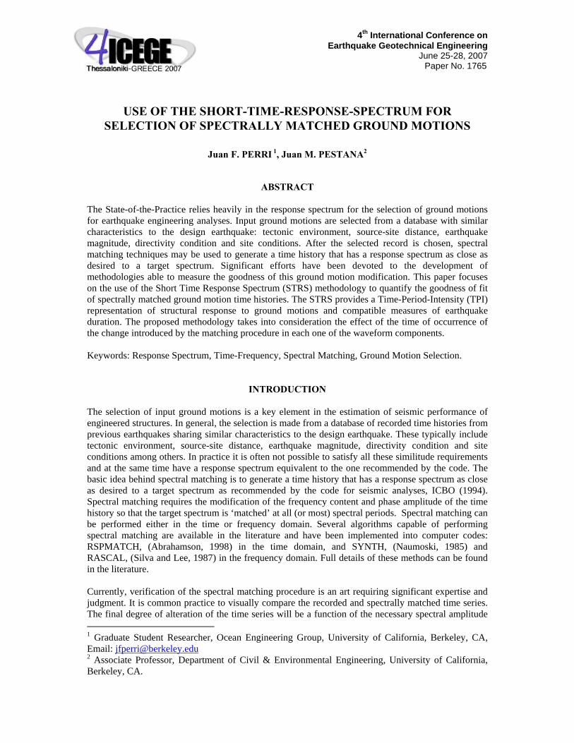
freedom system subjected to a seismic input motion. This methodology was used by Perez (1980) to develop spectra of amplitudes sustained for a given number of cycles. Other examples of the application of time-frequency analyses of seismic ground motions include the development of meaningful frequency-dependent duration (e.g. Novikova & Trifunac, 1993). More recently, Trifunac et al. (2001) studied the “apparent instantaneous frequency” of buildings and its long and short term variations. Wang et al. (2002) studied the effect of non-stationary motions on the non-linear response of a SDOF system and a frame structure. Other developments have focused on the modeling of the non-stationary amplitude and frequency evolution of synthetic ground motions (e.g. Der Kiureghian & Crempien, 1989; Conte & Peng, 1997). All these studies describe signal’s frequency and amplitude evolution in the time-frequency (or time-period) domain. Perri et al. (2005) proposed the Short Time Response Spectrum (cf., Appendix A) to obtain a Time-Period-Intensity representation of the non stationary structural response of a single degree of freedom system for a given ground motion. For a fixed structural damping, the pseudo-acceleration response spectrum is a plot of the maximum pseudo-acceleration experienced by the SDOF, as a function of the natural period, T, (or natural frequency). Perri et al. (2005) suggest the use of a period proportional Hanning window to evaluate the evolution in time of the maximum structural response. When this procedure is repeated for multiple ‘natural’ periods a Time-Period-Intensity picture emerges. Figure 1 shows the representation of the pseudo-acceleration short time response spectrum (STRSA) for the Sunnyvale Colton Avenue recording of the 1989 Loma Prieta earthquake.

Figure 1. 3D and 2D Time- Period-Intensity representation of the STRSA (Sunnyvale Colton

Avenue 360, Loma Prieta 1989 earthquake)

The projection of this three-dimensional plot into the spectral acceleration (Sa) – period (T) vertical plane produces the commonly used response spectrum. The projection in the time (t) – period (T) horizontal plane produces the recommended representation of the STRS (filled/color contour plot). All analyses and graphs presented in this paper use a 5% damping ratio for the response spectrum and Hanning window of length 5T for the computation of the STRS. Perri and Pestana (2006) proposed two period-dependent duration measures which can be directly obtained from the STRS analyses. The ‘Bracketed Duration Response Spectrum’ (BDRS) gives the Period dependent time interval between the first and last exceedances of a given threshold (e.g., 0.05g) while the ‘Cumulative Duration Response Spectrum’ (CDRS) is obtained by computing the cumulative time over which a particular threshold is exceeded. The spectral value of the CDRS is always less or equal than the BDRS. For most structural analyses, the CDRS is more relevant, since the nonlinear response of a structure is directly related to the duration in which an intensity level is exceeded. In contrast, the BDRS is more relevant for most site response analyses since the nonlinearity associated with excess pore pressures generated do not dissipate quickly enough to consider several peaks in the motion as ‘separate’ events. Perri and Pestana (2006) describe the detailed procedure for the calculation of the BDRS and CDRS, and show the results of several example applications of the two measurements (Perri and Pestana, 2006; Perri, 2007)

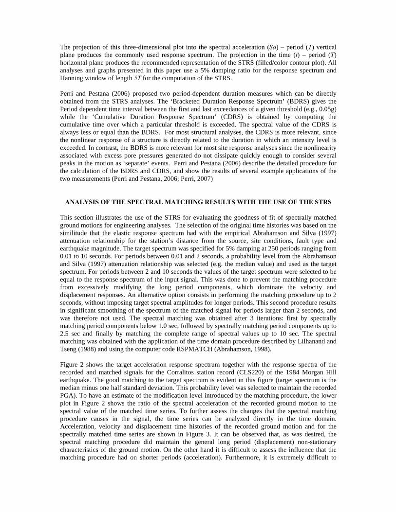
ANALYSIS OF THE SPECTRAL MATCHING RESULTS WITH THE USE OF THE STRS This section illustrates the use of the STRS for evaluating the goodness of fit of spectrally matched ground motions for engineering analyses. The selection of the original time histories was based on the similitude that the elastic response spectrum had with the empirical Abrahamson and Silva (1997) attenuation relationship for the station’s distance from the source, site conditions, fault type and earthquake magnitude. The target spectrum was specified for 5% damping at 250 periods ranging from 0.01 to 10 seconds. For periods between 0.01 and 2 seconds, a probability level from the Abrahamson and Silva (1997) attenuation relationship was selected (e.g. the median value) and used as the target spectrum. For periods between 2 and 10 seconds the values of the target spectrum were selected to be equal to the response spectrum of the input signal. This was done to prevent the matching procedure from excessively modifying the long period components, which dominate the velocity and displacement responses. An alternative option consists in performing the matching procedure up to 2 seconds, without imposing target spectral amplitudes for longer periods. This second procedure results in significant smoothing of the spectrum of the matched signal for periods larger than 2 seconds, and was therefore not used. The spectral matching was obtained after 3 iterations: first by spectrally matching period components below 1.0 sec, followed by spectrally matching period components up to 2.5 sec and finally by matching the complete range of spectral values up to 10 sec. The spectral matching was obtained with the application of the time domain procedure described by Lilhanand and Tseng (1988) and using the computer code RSPMATCH (Abrahamson, 1998). Figure 2 shows the target acceleration response spectrum together with the response spectra of the recorded and matched signals for the Corralitos station record (CLS220) of the 1984 Morgan Hill earthquake. The good matching to the target spectrum is evident in this figure (target spectrum is the median minus one half standard deviation. This probability level was selected to maintain the recorded PGA). To have an estimate of the modification level introduced by the matching procedure, the lower plot in Figure 2 shows the ratio of the spectral acceleration of the recorded ground motion to the spectral value of the matched time series. To further assess the changes that the spectral matching procedure causes in the signal, the time series can be analyzed directly in the time domain. Acceleration, velocity and displacement time histories of the recorded ground motion and for the spectrally matched time series are shown in Figure 3. It can be observed that, as was desired, the spectral matching procedure did maintain the general long period (displacement) non-stationary characteristics of the ground motion. On the other hand it is difficult to assess the influence that the matching procedure had on shorter periods (acceleration). Furthermore, it is extremely difficult to

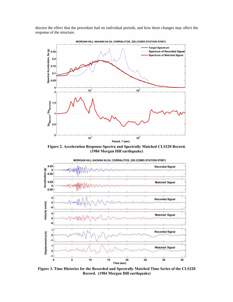
discern the effect that the procedure had on individual periods, and how these changes may affect the response of the structure.

Figure 2. Acceleration Response Spectra and Spectrally Matched CLS220 Record.

(1984 Morgan Hill earthquake)

Figure 3. Time Histories for the Recorded and Spectrally Matched Time Series of the CLS220

Record. (1984 Morgan Hill earthquake)

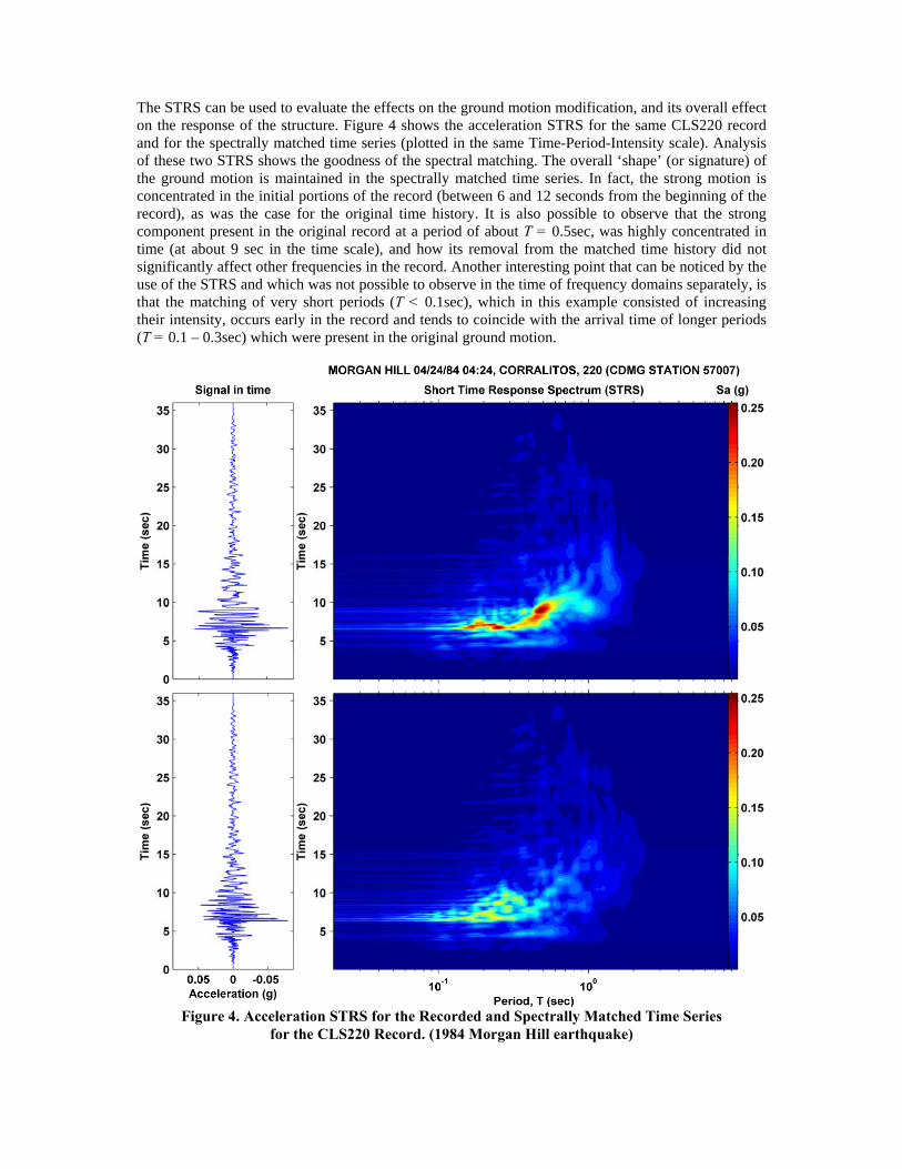
The STRS can be used to evaluate the effects on the ground motion modification, and its overall effect on the response of the structure. Figure 4 shows the acceleration STRS for the same CLS220 record and for the spectrally matched time series (plotted in the same Time-Period-Intensity scale). Analysis of these two STRS shows the goodness of the spectral matching. The overall ‘shape’ (or signature) of the ground motion is maintained in the spectrally matched time series. In fact, the strong motion is concentrated in the initial portions of the record (between 6 and 12 seconds from the beginning of the record), as was the case for the original time history. It is also possible to observe that the strong component present in the original record at a period of about T = 0.5sec, was highly concentrated in time (at about 9 sec in the time scale), and how its removal from the matched time history did not significantly affect other frequencies in the record. Another interesting point that can be noticed by the use of the STRS and which was not possible to observe in the time of frequency domains separately, is that the matching of very short periods (T < 0.1sec), which in this example consisted of increasing their intensity, occurs early in the record and tends to coincide with the arrival time of longer periods (T = 0.1 – 0.3sec) which were present in the original ground motion.

Figure 4. Acceleration STRS for the Recorded and Spectrally Matched Time Series

for the CLS220 Record. (1984 Morgan Hill earthquake)

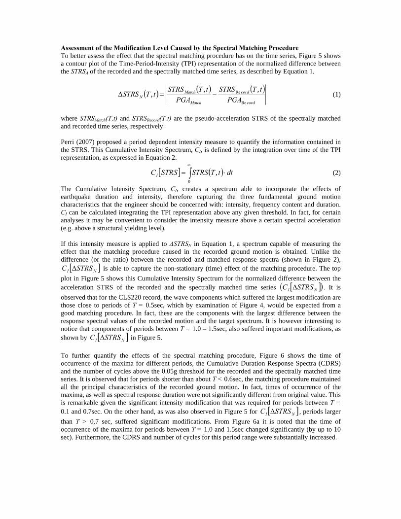
Assessment of the Modification Level Caused by the Spectral Matching Procedure To better assess the effect that the spectral matching procedure has on the time series, Figure 5 shows a contour plot of the Time-Period-Intensity (TPI) representation of the normalized difference between the STRSA of the recorded and the spectrally matched time series, as described by Equation 1.

( ) ( ) ( )cord

cord

Match

MatchN PGA

tTSTRSPGA

tTSTRStTSTRS

Re

Re ,,, −=Δ (1)

where STRSMatch(T,t) and STRSRecord(T,t) are the pseudo-acceleration STRS of the spectrally matched and recorded time series, respectively. Perri (2007) proposed a period dependent intensity measure to quantify the information contained in the STRS. This Cumulative Intensity Spectrum, CI, is defined by the integration over time of the TPI representation, as expressed in Equation 2.

[ ] ( )∫∞

⋅=0

, dttTSTRSSTRSCI (2)

The Cumulative Intensity Spectrum, CI, creates a spectrum able to incorporate the effects of earthquake duration and intensity, therefore capturing the three fundamental ground motion characteristics that the engineer should be concerned with: intensity, frequency content and duration. CI can be calculated integrating the TPI representation above any given threshold. In fact, for certain analyses it may be convenient to consider the intensity measure above a certain spectral acceleration (e.g. above a structural yielding level). If this intensity measure is applied to ΔSTRSN in Equation 1, a spectrum capable of measuring the effect that the matching procedure caused in the recorded ground motion is obtained. Unlike the difference (or the ratio) between the recorded and matched response spectra (shown in Figure 2),

[ ]NI STRSC Δ is able to capture the non-stationary (time) effect of the matching procedure. The top plot in Figure 5 shows this Cumulative Intensity Spectrum for the normalized difference between the acceleration STRS of the recorded and the spectrally matched time series [ ]( )NI STRSC Δ . It is observed that for the CLS220 record, the wave components which suffered the largest modification are those close to periods of T = 0.5sec, which by examination of Figure 4, would be expected from a good matching procedure. In fact, these are the components with the largest difference between the response spectral values of the recorded motion and the target spectrum. It is however interesting to notice that components of periods between T = 1.0 – 1.5sec, also suffered important modifications, as shown by [ ]NI STRSC Δ in Figure 5. To further quantify the effects of the spectral matching procedure, Figure 6 shows the time of occurrence of the maxima for different periods, the Cumulative Duration Response Spectra (CDRS) and the number of cycles above the 0.05g threshold for the recorded and the spectrally matched time series. It is observed that for periods shorter than about T < 0.6sec, the matching procedure maintained all the principal characteristics of the recorded ground motion. In fact, times of occurrence of the maxima, as well as spectral response duration were not significantly different from original value. This is remarkable given the significant intensity modification that was required for periods between T = 0.1 and 0.7sec. On the other hand, as was also observed in Figure 5 for [ ]NI STRSC Δ , periods larger than T > 0.7 sec, suffered significant modifications. From Figure 6a it is noted that the time of occurrence of the maxima for periods between T = 1.0 and 1.5sec changed significantly (by up to 10 sec). Furthermore, the CDRS and number of cycles for this period range were substantially increased.

Figure 5. Cumulative Intensity Spectrum and Time-Period-Intensity Representation

of the ΔSTRSN for the CLS220 Record. (1984 Morgan Hill earthquake)

CONCLUSIONS The use of spectrally matched records to develop input ground motions for earthquake analyses continues to increase in engineering practice. The process generates a time series that has a response spectrum as close as desired to a target spectrum, as recommended by the code for seismic analyses, ICBO (1994). Although there are several algorithms available to perform spectral matching in time and frequency domains, there is a lack of a quantitative methodology to evaluate the goodness of fit. This paper uses the Short Time Response Spectrum (STRS) methodology, for determining the Time-Period-Intensity representation of structural response. In this paper, the STRS was used to analyze the effect that the spectral matching procedure has on the ground motion. An intensity spectrum was introduced and used to quantify the modifications made by the spectral matching procedure. It was observed that for the analyzed example, although significant modifications were made for the spectral amplitudes in the response spectrum, time of occurrence of the maxima and duration spectra for the recorded and modified time histories, were not significantly changed. This procedure has shown that the modified synthetic time series is able to match the target spectrum without significantly modifying the original ground motion. The decision of accepting or rejecting a spectrally matched time series is often made based on qualitative comparison of the recorded and modified time history. This paper has shown a procedure by which the modification level can be quantified, and therefore, help the engineer assess the appropriateness of the synthetic signal for design purposes. Further analyses are being carried out to propose limit levels of modification, measured by the Cumulative Intensity Spectrum, CI, which should not be exceeded by the spectral matching procedure. Nevertheless, the methodology proposed thus far is useful for discerning between competing matching procedures and/or methodologies by comparing the Cumulative Intensity Spectrum of the different ‘spectrally matched’ time series.

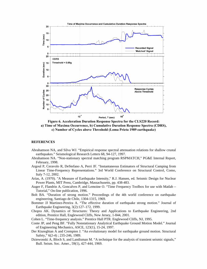
Figure 6. Acceleration Duration Response Spectra for the CLS220 Record:

a) Time of Maxima Occurrence, b) Cumulative Duration Response Spectra (CDRS), c) Number of Cycles above Threshold (Loma Prieta 1989 earthquake)

REFERENCES Abrahamson NA, and Silva WJ. “Empirical response spectral attenuation relations for shallow crustal

earthquakes.” Seismological Research Letters 68, 94-127, 1997. Abrahamson NA. “Non-stationary spectral matching program RSPMATCH,” PG&E Internal Report,

February, 1998. Argoul P, Ceravolo R, DeStefano A, Perri JF. “Instantaneous Estimators of Structural Camping from

Linear Time-Frequency Representations.” 3rd World Conference on Structural Control, Como, Italy 7-12, 2002.

Arias, A. (1970). "A Measure of Earthquake Intensity," R.J. Hansen, ed. Seismic Design for Nuclear Power Plants, MIT Press, Cambridge, Massachusetts, pp. 438-483.

Auger F, Flandrin A, Goncalves P, and Lemoine O. “Time Frequency Toolbox for use with Matlab – Tutorial,” On-line publication, 1996.

Bolt BA. “Duration of strong motion.” Proceedings of the 4th world conference on earthquake engineering, Santiago de Chile, 1304-1315, 1969.

Bommer JJ Martinez-Pereira A. “The effective duration of earthquake strong motion.” Journal of Earthquake Engineering, 3(2):127–172, 1999.

Chopra AK. Dynamics of Structures: Theory and Applications to Earthquake Engineering, 2nd edition, Prentice Hall, Englewood Cliffs, New Jersey, 1-844, 2001.

Cohen L. “Time-frequency analysis.” Prentice Hall PTR. Englewood Cliffs, NJ, 1995. Conte JP, and Peng BF. “Fully Nonstationary Analytical Earthquake Ground Motion Model.” Journal

of Engineering Mechanics, ASCE, 123(1), 15-24, 1997. Der Kiureghian A and Crempien J. “An evolutionary model for earthquake ground motion. Structural

Safety,” 6(2-4) ; 235-246, 1989. Dziewonski A, Bloch S, and Landisman M. “A technique for the analysis of transient seismic signals,”

Bull. Seism. Soc. Amer., 59(1), 427-444, 1969.

Hancock J, and Bommer JJ. “The effective number of cycles of earthquake ground motion.” Earthquake Engineering and Structural Dynamics, 34: 637-664, 2005.

Hubbard BB. “The world according to wavelets: the story of a mathematical technique in the making,” A.K. Peters. Wellesley, MA, 1998.

Husid LR. Caracteristicas de terremotos. Analisis general. Revista del IDIEM, 8, Santiago de Chile, 21-42, 1969.

ICBO. “Uniform Building Code,” International Conference of Building Officials, Whittier, California, 1994.

Jennings PC. “Ground motion parameters that influence structural damage,” in Strong ground motion simulation and engineering applications, Editors: Scholl R.E. & King J.L., EERI Publications 85-02, Earthquake Engineering Research Institute, Berkeley, California, 1985.

Joyner WB, and Boore DM. “Measurement, characterization, and prediction of strong ground motion.” Earthquake Engineering and Soil Dynamics II- Recent Advances in Ground Motion Evaluation Geotechnical Special Publication 20, ASCE 43-102, 1988.

Kawashima K and Aizawa K. “Earthquake response spectra taking account of number of response cycles.” Earthquake Engineering and Structural Dynamics, 14:185 –197, 1986.

Landisman M, Dziewonski A, Sato Y. “Recent improvements in the analysis of surface wave observations,” Geophys. J.Astron. Soc. 17, 369-403, 1969

Lilhanand K, and Tseng WS. “Development and Application of Realistic Earthquake Time Histories Comparable with Multiple Damping Design Spectra.” Proceeedings of the Ninth World Conference on Earthquake Engineering, Tokyo-Kyoto, Japan, Vol.2, 1988.

Malhotra PK. “Cyclic-demand spectrum.” Earthquake Engineering and Structural Dynamics, 31: 1441-1457, 2002.

Naumoski N. “SYNTH program: generation of artificial acceleration time history compatible with a target spectrum,” Dept. of Civil Engineering, McMaster Univ., Hamilton, Ont., Canada, 1985.

Nigam NC, and Jennings PC. “Digital Calculation of Response Spectra from Strong-Motion Earthquake Records,” Earthquake Engineering Research Lab., Cal. Institute of Technology, Pasadena, CA, 1968.

Novikova EI, and Trifunac MD. “Duration of Strong Earthquake Ground Motion: Physical Basis and Empirical Equations.” Report No. 93-02, Dept. of Civil Engrg., Univ. of Southern California, 1993.

Perez V. “Velocity response envelope spectrum as a function of time, for Pacoima Dam, San Fernando earthquake, February 9, 1971,” Bull. Seism. Soc. Amer., v. 63, 299-313. 1973.

Perri JF. “Numerical Modeling of Pile Installation Effects and Analyses of Strong Motion Loading on Engineering Structures.” Ph.D. Thesis, University of California, Berkeley, CA. 2007.

Perri, JF, and Pestana, JM. “Analyses of Ground Motions for Seismic Studies using the Short Time Response Spectrum”, GeoEngineering Research Report No. UCB/GE/2006, Dep. of Civil & Environ. Engng., UC Berkeley, November 2006.

Perri, JF, Bea, RB and Pestana, JM. “Short Time Response Spectrum,” Earthquake Engineering and Structural Dynamics. Submitted. 2006.

Perri, JF, Pestana, JM and Bea, RB. “Short Time Response Spectrum,” GeoEngineering Research Report No. UCB/GE/2005, Dep. of Civil & Environ. Engng., UC, Berkeley, June 2005.

Silva WJ, and Lee K. “WES RASCAL Code for Synthesizing Earthquake Ground Motions,” US Army Engineer Waterways Experiment Station, Report 24, Misc. Paper S-73-1, 1987.

Trifunac MD, and Brune JN. “Complexity of energy release during the Imperial Valley, California, earthquake of 1940.” Bull. Seism. Soc. Amer., 60, 137-160, 1970.

Trifunac MD, Ivanovic SS, and Todorovska MI. “Apparent periods of a building II: time-frequency analysis,” J. of Struct. Engrg, ASCE, 127(5), 527-537, 2001.

Trifunac MD. “Response Envelope Spectrum and Interpretation of Strong Earthquake Ground Motion.” Bull. Seism. Soc. Amer., 61, 343-356, 13, 1971.

Wang J, Fan L, Qian S, and Zhou J. “Simulations of non-stationary frequency content and its importance to seismic assessment of structures.” Earthquake Engineering & Structural Dynamics, 31.4, 993-1005, 2002.

APPENDIX A: SUMMARY OF THE SHORT-TIME-RESPONSE-SPECTRUM METHODOLOGY. The current State-of-the-Practice relies heavily on the use of the Elastic Response Spectrum (response spectrum for short) for assessing seismic demand on engineered structures. The response spectrum provides the maximum response that a single degree of freedom (SDOF) oscillator of given natural period and damping will exhibit when excited by an input ground motion. This tool is limited in the sense that it does not provide any information regarding the relative timing of the occurrence of the maxima, number of strong motion cycles or duration of this high intensity motion. The next section briefly summarizes the key elements of the Short-Time-Response-Spectrum methodology to obtain a Time-Period-Intensity (TPI) representation of the structural response of a single degree of freedom system subjected to a given ground excitation as presented by Perri et al (2005). The equation describing the relative motion x(t) of a single degree of freedom (SDOF) oscillator subjected to base acceleration )(txg&& is given by Equation (A1).

)()()(2)( 2 txtxtxtx goo &&&&& −=⋅+⋅⋅⋅+ ωωζ (A1) where ζ is the fraction of critical damping and ωo is the natural frequency of the SDOF oscillator. There are several methods available for the solution of this differential equation both in the frequency and time domains and they can be readily found in the literature (e.g., Nigam and Jennings 1968, Chopra 2001). For a given structural damping, the acceleration response spectrum is a plot of the maximum acceleration experienced by the SDOF, as a function of the natural period, T, (or natural frequency). For engineering applications, the pseudo-acceleration response spectrum is more frequently used, because it is directly related to the inertial force associated with the mass undergoing the acceleration. The pseudo-acceleration response spectrum is a plot of the quantity A(T,ζ) as a function of the natural vibration period, T, for a fixed damping, ζ (Equation A2).

);,(max2);,(max);(2

2 ζπζωζ TtxT

TtxTAtto ⋅⎟

⎠⎞

⎜⎝⎛=⋅= (A2)

Although considerable computational effort is required to generate the response spectrum, a significant amount of information is lost in the process. In order to preserve most of the information computed for the calculation of the response spectrum, and to present it in a tractable manner, the STRS can be used to decompose the input ground motion into a two-dimensional function of time and period (frequency) Given the response time history of a SDOF oscillator, it is possible to obtain a “local” maximum by windowing the response time history, ),;( ζτ Tx , around a particular instant (t) with a short time window, )( τ−th . Figure A1 shows conceptually the response of a SDOF oscillator (i.e., signal) to an input ground motion and the “windowed” signal [ )(),;( τζτ −⋅ thTx ] using a Hanning window of a given length. Using this procedure it is possible to determine the maximum of the windowed signal at a given time instant. By shifting the location of the short time window along the SDOF response time history, the “local” maxima can be recorded, and the time evolution of these maxima in the overall response is obtained (Equation A3).

∫ ⋅−⋅=t

dthTxhTtx0

max )(),;(max),,;( ττζτζτ

(A3)

If the analysis is repeated for all the desired SDOF oscillators, with a fixed structural damping, ζ, and window length and shape, h, the displacement STRS is obtained and is referred to as STRSD. As shown by Perri (2007), significant advantages are obtained when a period-proportional window length is selected. Using this period proportional window [i.e., );( Tth −τ ] the displacement, pseudo-velocity and pseudo-acceleration STRS become:

∫ ⋅−⋅=t

D dTthTxhTtSTRS0

);();,(max),;,( ττζτζτ

(A4a)

DDoV STRST

STRShTtSTRS ⋅⎟⎠⎞

⎜⎝⎛=⋅=πωζ 2),;,( (A4b)

DDoA STRST

STRShTtSTRS ⋅⎟⎠⎞

⎜⎝⎛=⋅=

22 2),;,( πωζ (A4c)

where STRSD, STRSV and STRSA, refer to the Time-Period-Intensity (TPI) representation of the displacement, pseudo-velocity and pseudo-acceleration time histories respectively (tSTRSV and tSTRSA will be used for the STRS of the total velocity and total acceleration, respectively). Perri et al. (2005) show results supporting the use of a period-proportional window length of approximately 5 times the natural period of interest. They analyzed several window shapes and showed that the results were not very sensitive to the type of window used. Based on those analyses, the final recommendation of their work is to use a Hanning window of length 5T.

Figure A1. Windowing of Response Time history: Original and Windowed Signal