use of two-segmented logistic regression to estimate change

American Journal of EpidemiologyCopyright O 1998 by The Johro Hopkins University School of Hygiene and Public HealthAll rights reserved

Vol. 148, No. 7Printed hi USA.

Use of Two-segmented Logistic Regression to Estimate Change-points inEpidemiologic Studies

Roberto Pastor and Eliseo GuaJlar

In many epidemiologic data, the dose-response relation between a continuous exposure and the risk ofdisease abruptly changes when the exposure variable reaches an unknown threshold level, the so-calledchange-point. Although several methods are available for dose-response assessment with dichotomousoutcomes, none of them provide inferential procedures to estimate change-points. In this paper, we describea two-segmented logistic regression model, in which the linear term associated with a continuous exposurein standard logistic regression is replaced by a two-segmented polynomial function with unknown change-point, which is also estimated. A modified, iteratively reweighted least squares algorithm is presented to obtainparameter estimates and confidence intervals, and the performance of this model is explored throughsimulation. Finally, a two-segmented logistic regression model is applied to a case-control study of theassociation of alcohol intake with the risk of myocardial infarction and compared with alternative analyses. Theability of two-segmented logistic regression to estimate and provide inferences for the location of change-points and for the magnitude of other parameters of effect will make this model a useful complement to othermethods of dose-response analysis in epidemiologic studies. Am J Epidemiol 1998;148:631-42.

case-control studies; epidemiologic methods; logistic models; risk assessment

Epidemiologic studies are often designed to explorethe relation between a continuous exposure variableand disease risk. Frequently, the dose-response rela-tion abruptly changes when the exposure variablereaches an unknown threshold level, the so-calledchange-point (1-5), but none of the usual methods ofdose-response analysis provides inference proceduresfor estimating the location of the change-point or itsconfidence interval.

In categorical analysis (6), the exposure range isdivided into a few categories (such as tertiles, quar-tiles, or quintiles), and then a constant disease risk isestimated within each category. Since the disease riskis forced to remain invariant within each category, thecutpoints between adjacent categories will determinein advance the points of risk change, and hence, cat-egorical analysis will be inefficient for detecting thelocation of the change-point. To avoid the limitationsof categorical analysis, spline regression can be used

Received for publication November 3, 1997, and accepted forpublication February 27, 1998.

Abbreviations: EURAMIC, EURopean study on Antioxidarrts,Myocardial Infarction, and breast Cancer; IRLS, iterativety re-weighted least squares; ML, maximum likelihood.

From the Department of Epidemiology and Biostatistics, NationalSchool of Public Health, Instituto de Salud Carlos III. Madrid, Spain.

Reprint requests to Dr. Roberto Pastor, Departamento de Epide-miologla y Bloestadfstica, Escuela NacionaJ de Sanidad, SinesioDelgado 8, 28029 Madrid, Spain.

to fit linear or quadratic models within each category(7-9). Spline regression allows the risk to changewithin categories, and it is more flexible in estimatingthe shape of the dose-response relation than is cate-gorical analysis, but the location of the knots has to befixed arbitrarily by the investigator. An alternativeapproach to exploring risk trend is to use nonparamet-ric logistic regression to display the dose-responserelation without parametric assumptions about the risktrend and without the need to categorize the continu-ous exposure variable (9, 10), but the identification ofchange-points with this method is subjective.

The aim of this paper is to introduce statisticalmethods for estimating change-points in epidemio-logic studies by using logistic regression. Severalmethods for change-point estimation have alreadybeen applied to explore the relation between two con-tinuous variables, including two-segmented polyno-mial regression models (1). The approach presentedhere is an adaptation of these models to data with adichotomous response variable. A related method hasbeen developed for detecting J-shaped risk curves inproportional hazards models (11), but this method didnot provide an algorithm for simultaneous estimationof all model parameters. In this paper, we describe themain theoretic properties of the proposed model anddevelop inference procedures to obtain simultaneousestimates of the change-point and associated parame-

631

Dow

nloaded from https://academ

ic.oup.com/aje/article/148/7/631/148349 by guest on 27 N

ovember 2021

632 Pastor and Guallar

ters. We also present the results of a simulation studyto explore the appropriateness of using large-sampleapproximations for model inferences. Finally, weshow the epidemiologic applicability of this model ina case-control study of the association of alcohol in-take with the risk of myocardial infarction.

For concreteness, we shall consider a case-controlstudy in which the dichotomous response variable ydenotes each patient's disease status (y = 1 for casesand y = 0 for controls). For each subject, we have a setof p + 1 risk factors or covariates x, zx, . .., zp. Theinterest is focused on a single continuous exposurevariable x, and the remaining risk factors are possibleconfounders for the association between exposure anddisease.

TWO-SEGMENTED LOGISTIC REGRESSION

The principal objective of the logistic regressionmodel presented here is to estimate a potential change-point in the exposure variable x at which the shape ofthe dose-response relation markedly changes. To ad-dress this problem, we propose replacing the linearterm associated with the exposure x in standard logis-tic regression by a two-segmented polynomial func-tion with unknown change-point. That is, the paramet-ric relation between the logit (i.e., the naturallogarithm of disease odds) and the continuous expo-sure variable x is assumed to follow two differentpolynomial forms on either side of an unknownchange-point. The model, here termed two-segmentedlogistic regression, can be expressed in terms of thelogit

TTJX, ZU • • • , Zp)

= f{x,X)

(1)

where TT(X, zu ..., zp) = P(y = l\x, zu • • ., zp) denotesthe probability of disease for a given set of covariates,A is the unknown change-point, the two-segmentedpolynomial function is f(x, A) = fx(x) if x < A andf2(x) otherwise, with fx(x) and f2(x) being differentpolynomials, and ax, . . ., ap are the regression coef-ficients of the remaining covariates. For practical ap-plications, one must specify the order of the polyno-mials (such as linear, quadratic, or cubic). Thedesirable property of smooth transition at the change-point requires one of the polynomials to be at leastquadratic. On the other hand, the coefficients of poly-nomials of order greater than quadratic will be difficultto interpret in epidemiologic or biologic terms. Themain alternatives for two-segmented logistic regres-

sion are thus linear-quadratic, quadratic-linear, orquadratic-quadratic models. In the next section, wedescribe the properties and applications of the linear-quadratic logistic regression model (linear below andquadratic above the change-point), but inferences withrespect to other two-segmented logistic models aresimilar, and the algorithms described in appendix 1also apply to all model alternatives.

Linear-quadratic logistic regression

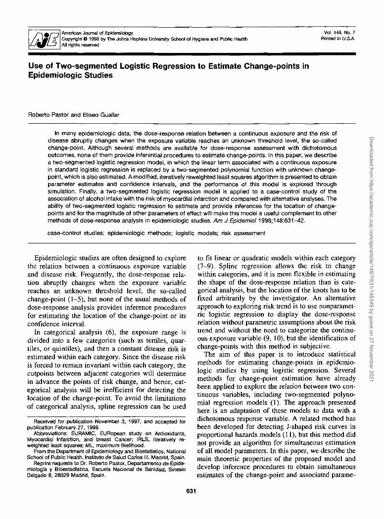
The two-segmented logistic regression with linear-quadratic form in the logit (figure 1) can be expressedas

g(x,

OLpZp, (2)

where A represents the unknown change-point; /30, /3j,and /32 are the unknown regression coefficients of theexposure variable x; and / ^ ^ = 1 if x > A and 0otherwise. In the two-segmented model with linear-quadratic logit, the effect is linear in the logit belowthe change-point A. In this segment, the logit is /30 +Pxx, where /30 is the intercept and /3, is the constantslope of the dose-response relation. Above the change-point A, the effect is quadratic in the logit and is givenby /30 + /3,x + (32(x - A)2, where /32 represents halfthe change in the slope of the logit per unit of incre-ment in exposure above the change-point. Since thederivative of the logit is continuous in this model,there is a smooth transition of the risk trend across thetwo segments: The slope is /3, below the change-point,and it begins to change in a continuous way above thechange-point according to the linear expression /S, +2/32 (x - A).

To fit the linear-quadratic logistic regression modelin equation 2, we must estimate the change-point A,and the regression coefficients of the exposure 0O, /3,,and /32

a nd °f the other covariates a,, . . ., ap. Themaximum likelihood (ML) estimates of these un-known parameters are those values, X, $0, folf $2>

a r |da,, . . . , 6tp, which maximize the log-likelihood func-tion

€ - log(L)

- 2 [y,g, -1-1

(3)

Am J Epidemiol Vol. 148, No. 7, 1998

Dow



ovember 2021

Two-segmented Logistic Regression 633

o

(a)

enO

a

(b)

FIGURE 1. Logit (a) and its derivative (b) In a linear-quadratic logistic regression model.

where y,- denotes the disease status for the ith subject,and TT,- = TT(X,., zn, • • •, zip) and g, = #(*,-, z,,, . . . , zip)are the probability of disease and its logit for the ithsubject, respectively. Since the logit (equation 2) is notlinear in the parameters and the change-point is notfixed in advance, the standard iteratively reweightedleast squares (IRLS) procedure (12) is inappropriate tofit tiiis model. Instead, we propose a modified versionof the IRLS procedure to estimate simultaneously allmodel parameters (a detailed presentation of this al-gorithm is provided in appendix 1).

Inferences in standard regression are usually con-

ducted using Wald-type approaches, based on the as-ymptotic normal distribution of the ML estimates, orLikelihood-based methods, directly obtained from theasymptotic x2 distribution of the likelihood ratio sta-tistic. In two-segmented regression, these asymptoticproperties depend on the existence of an underlyingchange-point (the so-called identified case) (2, 13). Aformal test for the existence of a change-point wouldbe represented by the null hypothesis Ho: /32 = 0,which implies an homogeneous linear pattern of dose-response. This situation, the nonidentified case, repre-sents a degeneracy of the parameter space: if /^ = 0,


Dow



ovember 2021


A is not well defined. In this case, the ML estimates arenot asymptotically normal, and the asymptotic distri-butions of the Wald and likelihood ratio statistics donot converge to standard normal and x2 distributions,respectively (3). All inferences described in this paper,such as confidence intervals or tests of hypothesis, arebased on the assumption of existence of A.

The Wald-type 100(1 - a) percent confidenceinterval for A can be estimated as X ± zl_a/2s(k),where Zy-a^ is the 100(1 - a/2) percentile of the stan-dard normal distribution and s<X) is an estimate of thestandard error obtained from the inverse of the Fisherinformation matrix at the last iteration of the modifiedIRLS algorithm (see appendix 1). However, thismethod yields a symmetric interval that is often inap-propriate due to the asymmetric distribution of thechange-point estimator (see Simulation Study). Moreappropriate confidence intervals for A can be obtainedby using the likelihood ratio statistic AA = 2€(X, £0,ft, &) - 2€(A, £0(A), £,(A), £2(A)), where fyk) isthe ML estimate of /3y given A (j = 0, 1, 2) (4). Thelikelihood-based 100(1 — a) percent confidence inter-val consists of those values A verifying Ak ^ xz

1 ,_ a ,where A^i,i-a represents the 100(1 - a) percentile ofthe x* distribution with 1 degree of freedom. Thisinterval is usually more accurate in terms of coveragethan is that based on the Wald approach.

SIMULATION STUDY

A simulation study was conducted to examine theproperties of the parameter estimates in the linear-quadratic logistic regression model. We considered asingle exposure variable that followed an uniformdistribution in the range 0 ^ x ^ 1. The exposure levelof each subject was randomly generated from thisdistribution, and the disease status was randomly as-signed according to the conditional probability of dis-ease given by

(4)

corresponding to a linear-quadratic logistic model withunderlying parameters A, /30, 0,, and Z^, equal to 0.75,—5, 0, and 30, respectively. In this model, the actualodds ratio for an exposure level x compared with thereference exposure level (x = 0) was constant andequal to 1 (no effect) below the threshold 0.75, and itincreased above this threshold with odds ratios of 1.08,1.35, 1.96, and 3.32 for exposure levels 0.80, 0.85,0.90, and 0.95, respectively. The data of the hypothet-ical case-control study consisted of the first 500 casesgenerated by this procedure and a random sample of500 controls from all of the available disease-freesubjects. A total of 1,000 replicates of the case-controlstudy were performed in the simulation.

For each of the 1,000 replicates, a linear-quadraticlogistic regression model was fitted to obtain theML estimates X, $0, &, and $2 using the GAUSSmatrix language (14). Several measurements of biasand accuracy of the sampling distributions of X, $v

and $2 a r e given in table 1. The distribution of thechange-point estimates was skewed to the left with amean of 0.735 and a median of 0.750 (mean andmedian bias of -0.015 and 0.0002, respectively). Themedian bias, that is, the difference between the medianof the sampling distribution of X and the true param-eter A, is a more general measure of bias for asym-metric distributions (15). Thus, although X wasslightly mean biased due to its asymmetric distribu-tion, it had the desirable property of being medianunbiased in our simulation study. The distribution ofthe estimates $, was close to a normal distribution,with a mean bias of —0.074 and a median bias of—0.027. The distribution of $2, however, was mark-edly right-skewed, with a median bias (1.01) that wasconsiderably smaller than its mean bias (18.69), in-flated by the asymmetric distribution of the estimates.

Even though the sample size of this hypotheticalcase-control study was moderate (500 cases and 500controls), the sampling distributions of the parameterestimates were not well approximated by the normal,and there were substantial differences between thepercentile-based confidence intervals (the 2.5th and97.5th empirical percentiles of the sampling distribu-

TABLE 1. Description of parameter estimates from the linear-quadratic logistic regression model applied to the 1,000 replicatesof the hypothetical case-control study

ParameterUnderlying

value Mean Standarddeviation

95%normal

tterval*Medbn Interquartile

range

95%percentleWervalt

X 0.75 0.735 0.110 0.519 to 0.950 0.750 0.096 0.467 to 0.887P, 0 -0.074 0.487 -1.028 to 0.881 -0.027 0.488 -0.978 to 0.624Pj 30 48.692 115.090 -176.885 to 274.269 31.013 28.563 6.630 to 167.827

* Mean ± 1.96 standard error.t Defined by the 2.5th and 97.5th percentites of the sampling distribution, respectively.


Dow



ovember 2021


tions (15)) and the standard nonnal confidence inter-vals (table 1).

To evaluate further the large sample approximation

of Wald and likelihood-based inferences for testingA = 0.75, /3, = 0, and /32 = 30, the Wald statisticsWA = (A - 0.75)/s(A), Wi - j&i/s(#i). and W2 -

Quontiles of standard normal

(a)

o:> ia

o.Eu

OuontDes of standard normol

(b)

Ouorttiles of standard normal

(C)

Ouontiles of standard normal

(d)

Quanltes of standard normal

•• 1

J

0 «•

OuontBes of standard normal

(e) (f)

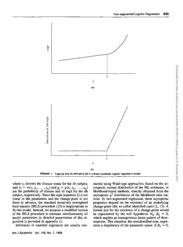
RGURE 2. Quantlle-quantile plots of the Wald statistics WA = (A - 0.75)/s(A) (a), W, = /ysfj*,) (c), and W2 = (Jj - 30)/s<jy (e), andof the signed square root of the likelihood ratio statistics LRt = sgn(A - 0.75) VA i_ 0 7 s Ip), LR, = sgntf,) VAP).O (d), and LR^ =sgn(J2 - 30) VAfc_3o (/) based on the 1,000 replicates of the simulation study.


Dow



ovember 2021


(£2 "~ 30)/s(£2), and the signed square root of thelikelihood ratio statistics LRA = sgn(X — 0.75)

VATZO, and LR, =VAA_0.75> LR, =0,-o>

sgn 02 ~ 30) VA^T^o w e r e computed for each rep-licate of the simulation study (4). The quantile-quan-tile plots for the statistics show that the samplingdistribution of Wl was close to the standard normal(figure 2c), while the sampling distributions of WK andW2 were highly skewed to the right and to the left,respectively (figures 2a and 2e). The sampling distri-butions of LRA, LR,, and LR2 were well approximatedby the standard normal (figures 2b, 2d, and 2f), show-ing that inferences based on the likelihood ratio sta-

tistics were more reliable than those based on Waldstatistics in our simulation. Similar results wereobtained in terms of coverage of the Wald and likeli-hood-based confidence intervals (not shown).

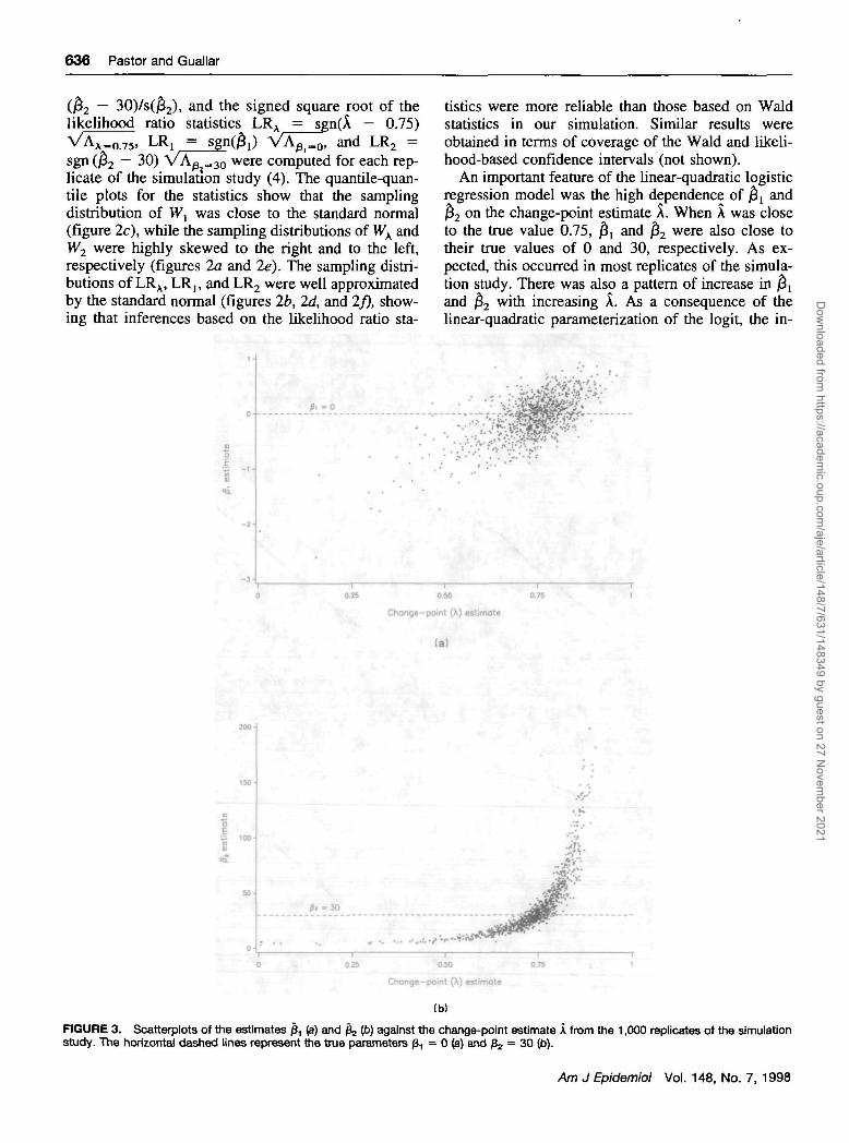
An important feature of the linear-quadratic logisticregression model was the high dependence of j5, and$2 on the change-point estimate X. When X was closeto the true value 0.75, $, and $2 were also close totheir true values of 0 and 30, respectively. As ex-pected, this occurred in most replicates of the simula-tion study. There was also a pattern of increase in $,and £2 with increasing X. As a consequence of thelinear-quadratic parameterization of the logit, the in-

I .,

(

/ ""

0.25 0 50

Change-point (A) estimote

(a)

I .00

O 0.25 0M 0.75 , 1

Change-point (X) estimate

FIGURE 3. Scatterplots of the estimates £, (a) and fe Ip) against the change-point estimate A from the 1,000 replicates of the simulationstudy. The horizontal dashed lines represent the true parameters /3, = 0 (a) and ft, = 30 (b).


Dow



ovember 2021


creasing pattern of £, was additive, while the increas-ing pattern of ^ was multiplicative (figure 3).

Additional simulation studies were performed withmodifications of the location of the change-point, theshape of the distribution of the exposure variable, andthe sample size, but the conclusions with respect tothe performance of model estimators were essentiallyunchanged.

EXAMPLE: ALCOHOL INTAKE AND RISK OFMYOCARDIAL INFARCTION IN THEEURAMIC STUDY

A two-segmented logistic regression model wasused to study the association of alcohol intake andrisk of myocardial infarction using data from theEURAMIC (EURopean study on Antioxidants, Myo-cardial Infarction, and breast Cancer) Study, an inter-national case-control study conducted in eight Euro-pean countries and Israel, designed primarily toevaluate the association of antioxidants with the risk ofdeveloping a first myocardial infarction in men. Themethods of the EURAMIC Study have been describedin detail elsewhere (16, 17). Cases were men aged lessthan 70 years with a confirmed diagnosis of first acutemyocardial infarction who had been admitted to thecoronary care units of participating hospitals within 24hours of the onset of symptoms. Controls were ob-tained through random samples of the population fromwhich the cases originated (five countries), throughrandom samples of the patients of the cases' generalpractitioners (one country), by inviting friends or rel-atives of the cases (one country), or through mixedmethods (two countries).

To focus on the dose-response of alcohol intake andrisk of myocardial infarction, we restricted our analy-ses to the 330 cases and 441 controls who reportedsome alcohol intake during the previous year, but theanalyses of all study subjects with additional indicatorvariables for ex-drinkers and never drinkers (18, 19)gave virtually the same results (not shown).

Among controls who were current drinkers, alcoholintake ranged from 0.1 to 142.6 g/day, and the 25th,50th, and 75th percentiles of intake were 5.7, 13.7,and 30.0 g/day, respectively. We fitted the follow-ing quadratic-linear logistic regression model to theEURAMIC Study alcohol data:

g(x, z , , . . . , zl6) =

a,z, (5)

where x represented alcohol intake in g/day, A was thechange-point, and the adjustment covariates zx,..., z l 6

were age, study center (eight indicator variables),smoking (current number of cigarettes smoked and

TABLE 2. Parameter estimates from the quadratic-linearlogistic regression model summarizing the association ofalcohol intake and risk of myocardial infarction in theEURAMIC Study*

ParameterPoim

UteHhood-based95% confidence

Interval

i

Pi

13.1180.0080.009

4.679 to 50.0620.000 to 0.0210.001 to 0.084

* Adjusted for age, center, smoking, waist-hip ratio, history ofdiabetes, history of hypertension, and family history of coronaryheart disease.

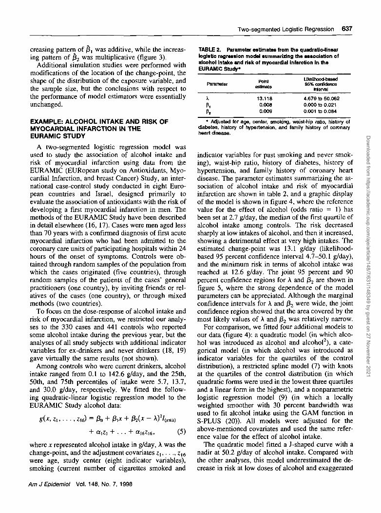
indicator variables for past smoking and never smok-ing), waist-hip ratio, history of diabetes, history ofhypertension, and family history of coronary heartdisease. The parameter estimates summarizing the as-sociation of alcohol intake and risk of myocardialinfarction are shown in table 2, and a graphic displayof the model is shown in figure 4, where the referencevalue for the effect of alcohol (odds ratio = 1) hasbeen set at 2.7 g/day, the median of the first quartile ofalcohol intake among controls. The risk decreasedsharply at low intakes of alcohol, and then it increased,showing a detrimental effect at very high intakes. Theestimated change-point was 13.1 g/day (likelihood-based 95 percent confidence interval 4.7-50.1 g/day),and the minimum risk in terms of alcohol intake wasreached at 12.6 g/day. The joint 95 percent and 90percent confidence regions for A and /32 are shown infigure 5, where the strong dependence of the modelparameters can be appreciated. Although the marginalconfidence intervals for A and /32 were wide, the jointconfidence region showed that the area covered by themost likely values of A and /32 was relatively narrow.

For comparison, we fitted four additional models toour data (figure 4): a quadratic model (in which alco-hol was introduced as alcohol and alcohol2), a cate-gorical model (in which alcohol was introduced asindicator variables for the quartiles of the controldistribution), a restricted spline model (7) with knotsat the quartiles of the control distribution (in whichquadratic forms were used in the lowest three quartilesand a linear form in the highest), and a nonparametriclogistic regression model (9) (in which a locallyweighted smoother with 30 percent bandwidth wasused to fit alcohol intake using the GAM function inS-PLUS (20)). All models were adjusted for theabove-mentioned covariates and used the same refer-ence value for the effect of alcohol intake.

The quadratic model fitted a J-shaped curve with anadir at 50.2 g/day of alcohol intake. Compared withthe other analyses, this model underestimated the de-crease in risk at low doses of alcohol and exaggerated


Dow



ovember 2021


5-

1/1"O"OO

2-

1 -

0.5-

0.2-

> Quadratic

Nonparametric

Spline

Quadratic-linear

Categorical

25 50 75 100 125 150

Alcohol intake (g/day)

FIGURE 4. Dose-response relation of alcohol intake to risk of myocardial Infarction estimated from five alternative models (quadratic,categorical, restricted spline, nonparametric, and quadratic-linear logistic regression models). Odds ratios were adjusted for age, center,smoking, waist-hip ratio, history of diabetes, history of hypertension, and family history of coronary heart disease, and the reference value(odds ratio = 1) was set at 2.7 g/day, the median of the first quartile of alcohol intake among controls. See text for details of the models.

the increase at higher doses. The categorical analysisshowed an L-shaped dose-response, with reduced andvery similar risk in die three highest quartiles. Finally,the quadratic-linear, spline, and nonparametric modelsresulted in a similar shape of the dose-response rela-tion, but only the quadratic-linear model providedinference procedures for the change-point.

DISCUSSION

In this paper, we have presented a two-segmentedlogistic regression model to estimate change-pointswith a dichotomous dependent variable, and we haveshown how to obtain point estimates and confidenceintervals for model parameters without the need todetermine in advance die approximate location of thechange-point.

Several regression models have been proposed toexplore the shape of the risk trend in dose-responseanalysis. Fractional polynomial regression (containingfractional and inverse powers of x, such as x~2, x~ ,x~I/2, x1/2, x, and x2) and spline regression are flexibleenough to reproduce a wide variety of dose-response

curves and can be easily programmed with standardstatistical software (7). In addition to these parametricmodels, nonparametric regression provides smoothcurves that summarize the exposure-disease relationwithout imposing any parametric assumption (10). Ifthere is a change-point in the effect of the exposure, itwill be reflected in the plots of the dose-responsecurves estimated from the above regression models. Avisual examination of these curves is commonly usedto approximately locate the change-point, but thispractice is largely subjective and does not provide asystematic inferential procedure for change-point es-timation. On the other hand, the two-segmented logis-tic regression model estimates simultaneously the lo-cation of the change-point and other parameters ofeffect of the exposure variable, avoiding the need forarbitrary cutpoints.

For practical applications, one of the most importantconsequences of two-segmented logistic regression isderived from the high dependence of the coefficientsof effect of the exposure, /3X and fa, with the change-point A (figures 3 and 5). The estimates of /3, and,


Dow



ovember 2021


0.15-

01 -

0 05-

0-—r~10 20 30

—r~40 50

Change-point (X)

FIGURE 5. Likelihood-based 90% and 95% confidence regions for (A, 0 J for the association of alcohol Intake and risk of myocardialinfarction in the EURAMIC Study. The plus sign (+) represents the ML estimate A = 13.118, and fe = 0.009.

especially, of /32 will be strongly dependent on thevalue of A. In other epidemiologic analyses involvingcategorization of the exposure range, the effect esti-mates will depend on the arbitrary position of thecutpoints, particularly in extreme categories of expo-sure. Thus, caution must be used in the interpretationof relative risks obtained after post hoc categorizationof the range of the exposure variable.

An additional consequence of categorizing the ex-posure is that the standard errors of the coefficients ofeffect will be artificially reduced in categorical orspline analyses. In our alcohol example, fitting thequadratic-linear spline model with a single knot at13.118 g/day of alcohol (the estimated change-point intwo-segmented regression),

+ 02(;t-13.118)2/Crii3.n8)

+ atz\ + . . . + al6zl6, (6)

resulted in the same parameter estimates $, and $2,but estimated with higher precision. For instance, thelikelihood ratio-based 95 percent confidence intervalfor /32 in the spline model was 0.005-0.013, substan-tially smaller than the confidence interval in ourquadratic-linear model, 0.001-0.084. This increasedprecision, however, was artificial in the sense that thespline model assumed a fixed, preestablished knot.The impact of the position of the change-point on

parameter estimates and the need to obtain realisticestimates of error highlight the need to develop modelsfor change-point estimation.

The two-segmented logistic regression model pro-vides valuable methods to estimate effects in certaindose-response analyses, but this approach is not with-out limitations. First, model inferences are based onthe assumption of existence of a change-point. Al-though a graphic examination of this assumption canbe performed by nonparametric logistic regression,further work is needed to adapt tests of hypothesisuseful when there is a degeneracy of the parameterspace under the null (21, 22) to segmented logisticregression models.

Second, as in other parametric models, the potentialfor model misspecification is always a problem (23).Nonparametric models are useful to check the appro-priate parameterization of the segmented model. Al-though we have restricted our presentation to a two-segmented polynomial function, these methods(including the algorithms described in appendix 1)also apply to other parametric forms of the logit and tomore than one change-point as long as the transitionsamong the segments are smooth. For continuous out-comes, segmented models have been extended toavoid the restriction of continuity at the change-points(24) or to impose continuity, but not derivability,across the transitions (13, 25-27). These methods in-cluded the particular case of two intersecting straight


Dow



ovember 2021


lines with a sharp comer at the change-point, whichwas later generalized to accommodate a smooth tran-sition, as well as an abrupt change using transitionfunctions in the neighborhood of the change-point(28). These generalizations, however, are not availablefor discrete outcomes. A segmented model has alsobeen developed for the detection of J-shaped riskcurves in proportional hazards models by obtainingthe profile log-likelihood from sequential quadraticspline models at different cutpoints (11), but thismethod did not provide an algorithm for simulta-neous estimation of the change-point and associatedparameters.

Third, we have explored the performance of modelestimators through simulation, but the results of oursimulation study may not be representative of whatmight occur in practice. Further simulation scenarioshave to be evaluated to assess adequately the appro-priateness of large-sample approximations for modelinferences (29).

Finally, the lack of availability of two-segmentedmodels in standard statistical packages restricts theirwidespread use at the moment. GAUSS macrosfor linear-quadratic, quadratic-linear, or quadratic-quadratic logistic regression are available upon requestby mail from the corresponding author or by electronicmail ([email protected]).

Our analysis of the alcohol data in the EURAMICStudy further illustrates the limitations of traditionaldose-response analysis in epidemiologic studies. Adose-response meta-analysis of alcohol intake and riskof myocardial infarction found an L-shaped associa-tion, described as a drop in risk at low doses, followedby a plateau in risk above one drink per day (30). Thecase-control studies combined in this meta-analysisbased their assessment of the effect of alcohol oncategorizations of alcohol intake, and their dose-response curves were very similar to our categoricalanalysis of the EURAMIC data. It is likely that the useof broad categories limited the ability of these studiesto detect an increased risk of myocardial infarction athigh intakes.

As previous studies (7, 11, 19) have also shown, theusual epidemiologic approach to dose-response assess-ment based on quadratic models or on categoricalanalysis will often be inadequate. As a minimumcheck, spline or nonparametric regression should beused to confirm more traditional methods. If theseanalyses provide evidence of abrupt changes in risk orif there are a priori reasons to suspect the existence ofchange-points, two-segmented logistic regressioncould then be used to estimate the change-point and toprovide more realistic measures of statistical error.

ACKNOWLEDGMENTS

Dr. Roberto Pastor was supported by a grant from the"Institute de Salud Carlos HT' (FIS 97/4148). Dr. EliseoGuallar's work was supported in part by grant FIS 95/0457.

The authors thank the EURAMIC Study group (ProfessorFrans Kok, Principal Investigator) for providing the originaldata for the example of alcohol intake and risk of myocar-dial infarction presented in this paper, and Drs. LeonGordis, Vfctor Moreno, lavier Nieto, and Santiago Perez-Hoyos for their helpful comments on earlier versions of thispaper.

REFERENCES

1. Gallant AR, Fuller WA. Fitting segmented polynomial regres-sion models whose join points have to be estimated. J Am StatAssoc 1973;68:144-7.

2. Feder PI. On asymptotic distribution theory in segmentedregression problems—identified case. Ann Stat 1975;3:49-83.

3. Feder PI. The log-likelihood ratio in segmented regression.Ann Stat 1975;3:84-97.

4. Zhan M, Dean CB, Routledge R, et al. Inference on segmentedpolynomial models. Biometrics 1996;52:321-7.

5. Seber GAF, Wild CJ. Nonlinear regression. New York, NY:John Wiley & Sons, 1989.

6. Breslow NE, Day NE, eds. Statistical methods in cancerresearch. Vol. 1. The analysis of case-control studies. Lyon,France: International Agency for Research on Cancer, 1980.

7. Greenland S. Dose-response and trend analysis inepidemiology: alternatives to categorical analysis. Epidemiol-ogy 1995;6:356-65.

8. Witte JS, Greenland S. A nested approach to evaluating dose-response and trend. Ann Epidemiol 1997;7:188-93.

9. Hastie TJ, Tibshirani RJ. Generalized additive models. Lon-don, England: Chapman & Hall, 1990.

10. Zhao LP, Kristal AR, White E. Estimating relative risk func-tions in case-control studies using a nonparametric logisticregression. Am J Epidemiol 1996; 144:598-609.

11. Goetghebeur E, Pocock SJ. Detection and estimation of J-shaped risk-response relationships. J R Stat Soc [A] 1995; 158:107-21.

12. McCullagh P, Nelder JA. Generalized linear models. London,England: Chapman & Hall, 1989.

13. Lerman PM. Fitting segmented regression models by gridsearch. Appl Stat 1980;29:77-84.

14. Aptech Systems, Inc. GAUSS. Vol. II. Command reference.Maple Valley, WA: Aptech Systems, Inc., 1993.

15. Efron B, Tibshirani RJ. An introduction to the bootstrap.London, England: Chapman & Hall, 1993.

16. Kardinaal AFM, Kok FJ, Ringstad J, et al. Ann'oxidantsin adipose tissue and risk of myocardial infarction: theEURAMIC Study. Lancet 1993;342:1379-84.

17. Kardinaal AFM, Kok FJ, Kohlmeier L, et al. Associationbetween toenail selenium and risk of acute myocardial infarc-tion in European men: the EURAMIC Study. Am J Epidemiol1997; 145:373-9.

18. Greenland S, Poole C. Interpretation and analysis of differen-tial exposure variability and zero-exposure categories for con-tinuous exposures. Epidemiology 1995;6:326-8.

19. Robertson C, Boyle P, Hsieh C, et al. Some statistical con-siderations in the analysis of case-control studies when theexposure variables are continuous measurements. Epidemiol-ogy 1994^:164-70.

20. Statistical Science, Inc. S-PLUS reference manual, version3.2. Seattle WA: MathSoft, Inc., 1993.

21. Davies RB. Hypothesis testing when a nuisance parameter is


Dow



ovember 2021


present only under the alternative. Biometrika 1977;64:247-54.

22. Davies RB. Hypothesis testing when a nuisance parameter ispresent only under the alternative. Biometrika 1987;74:33-43.

23. Maldonado G, Greenland S. Interpreting model coefficientswhen the true model form is unknown. Epidemiology 1993;4:310-18.

24. Hawkins DM. Point estimation of the parameters of piecewiseregression models. Appl Stat 1976;25:51-7.

25. Hudson DJ. Fitting segmented curves whose join points haveto be estimated. J Am Stat Assoc 1966;61:1097-129.

26. Hinkley DV. Inference about the intersection in two-phaseregression. Biometrika 1969;56:495-504.

27. Hinkley DV. Inference in two-phase regression. J Am StatAssoc 1971,66:736-43.

28. Bacon DW, Watts DG. Estimating the transition between twointersecting straight lines. Biometrika 1971;58:525-34.

29. Maldonado G, Greenland S. The importance of critically in-terpreting simulation studies. Epidemiology 1997;8:453-6.

30. Maclure M. Demonstration of deductive meta-analysis: etha-nol intake and risk of myocardial infarction. Epidemiol Rev1993;15:328-51.

APPENDIX

In this appendix, we develop an algorithm to fit two-segmented logistic regression models with logit g(x,Z\,. • ., zp)

= f(x, A) + GtjZj + . . . + ot-pZp, where/(x, A) is a two-segmented polynomial function with continuousfirst partial derivatives over the entire parameter space. The linear-quadratic, f(x, A) = /30 + fixx + /32(x — A)2

xy quadratic-linear, f(x, A) = /30 + j3,jc + /32(x - \)2lix s A), and quadratic-quadratic, f(x, A) = /30 + /3t;c ++ fS3(x — A)2 Iix a. A), models are special parameterizations off(x, A). The primary objective is to obtain the

ML estimate 0 = (A, 0o, £i, . . ., $q, &J, . . ., dp) of the vector of unknown parameters 0 = (A, /3o, /3i, . . ., /39,ai, . .., ap) that maximizes the log-likelihood of the two-segmented logistic regression model

t ~ log(l (Al)1=1

The score vector u(0) = d£/dO, with elements

r=l,...,p (A2)1=1

can be calculated because gt has continuous first partial derivatives with respect to 0 over the entire parameterspace. Since E{y^) = •ni and vai y,-) = iti (1 — TT,), u(d) has expectation 0 and covariance matrix equal to theFisher information matrix 1(0), with elements

In(0) = {E{u{0)UT(0))}n = (A3)

where /re (B) is the (r, *)th element of 1(0) (r, s = 1, . . ., p + q + 2). The ML estimates 0 are obtained as thesolutions of the p + q + 2 likelihood equations u(Q) = 0. Since these equations are not linear in the parameters0, iterative methods must be used to obtain 0. The two-segmented logistic regression model can be fitted by usingthe Fisher scoring method (12). Let fl**5 be the current estimate of 0, with corresponding score vector u(ffk>) andFisher information matrix I(0k>). The new estimate 8**+ ° is derived from /(fl*®) {&k+ ° - &ky) - u(6?k)), which,after evaluating equations A2 and A3 at 0(k>, results in the following system of equations (r = 1 , . . . , p + q + 2)

/=•!

p+q+2

4-J i f\ ' = 0. (A4)


Dow



ovember 2021


Using the first-order Taylor series of gt around &k\ we have [dgJde\e(k>\T{0k+l) - &k)) = g,(*+1) - glk\ and

then equation A4 can be rewritten as (r = 1,... ,p + q + 2)

y,= 0, (A5)

which are the weighted least squares equations of a two-segmented regression with weights w/** = 7r,(i) (1 —TT/**) and response variables v,( } = g/*} + (v, - 7r/*))Av/*). Thus, 0**+T) can be calculated by fitting a weightedtwo-segmented regression model, in which the weight w/** and the response variable v/** depend on &** and,hence, must be recomputed at each iteration (iteratively reweighted least squares procedure (12)).

Since the two-segmented regression function g(6) has continuous first derivatives throughout the parameterspace, Hartley's modification of Gauss-Newton algorithm can be used to solve the weighted two-segmentedregression models (1, 4). Let &kJ) be an estimate of 0 at the /th iteration of the procedure nested in the kth stageof the primary iterative process. For each subject, the first-order Taylor series of e,(0) around 0kll) gives gt{0)= 80kJ)) + [dg/dO\(f*. »]T(0-&k-n), and the residual rt(k, /) = v/*> - g0k^) can be expressed as

r'(M) = [^f ( O - ^ + ei i = l , . . . , n (A6)

or in matrix form for all subjects rtk, I) = G(k, I) (0 — (fikll)) + e, where iik, I) is the residual vector and G(k, I)is a matrix with (i, r)th element dg/ddji^). The solution of this linearized regression model with diagonal matrixof weights W(k) — diagfir/*5 (1 — ir, )} can be obtained by using the ordinary weighted least squares method,so that the solution is d(k, 1) = [GT(k, l)W(k)G(k, Or'G^k, l)W(k)r(k, I). Following Hartley's modifiedGauss-Newton algorithm for segmented polynomial regression models (1), the next estimate 0(*>'+r) is given by(fik'l) + T)(k, l)d{k, I), where t]{k, I) is the scalar between 0 and 1 at which (fik- ° + r)d(k, I) minimizes theweighted sum of the errors of the two-segmented regression model.

Each of these iterative procedures is stopped when the relative change between 0 ( t / + 1 ) and &kJ) is negligible,and the last estimate is used as the starting value of the next iterative process &k+1). One must then recomputethe weight w,(*+1) and the response variable v/*+1) at 0(*+1), and fit again the weighted, two-segmentedregression model using the above iterative procedure. This process is repeated until convergence.

The choice of the initial estimate €f-a) is crucial to obtain a proper convergence of the algorithm presented inthis appendix because the log-likelihood function (equation Al) may possess local maxima. A good alternativeis to use the grid-search approach to obtain the initial estimate (13). The method determines in advance severalequally spaced points over the range of the exposure variable x. For each point, a spline logistic regression withtwo-segmented logit (7, 9) is fitted, and the log-likelihood is evaluated. The point at which the log-likelihoodreaches the highest value is used along with the remaining parameter estimates from the spline logistic regressionas initial values


Dow



ovember 2021

use of two-segmented logistic regression to estimate change

Documents