usefulness of bioclimatic models for studying … of bioclimatic models for studying climate change...

Usefulness of Bioclimatic Modelsfor Studying Climate Change

and Invasive Species

Jonathan M. Jeschkea,b and David L. Strayerb

aSection of Evolutionary Ecology, Department of Biology II,Ludwig-Maximilians-University Munich, Germany

bCary Institute of Ecosystem Studies, Millbrook, New York, USA

Bioclimatic models (also known as envelope models or, more broadly, ecological nichemodels or species distribution models) are used to predict geographic ranges of organ-isms as a function of climate. They are widely used to forecast range shifts of organismsdue to climate change, predict the eventual ranges of invasive species, infer paleoclimatefrom data on species occurrences, and so forth. Several statistical techniques (includinggeneral linear models, general additive models, climate envelope models, classificationand regression trees, and genetic algorithms) have been used in bioclimatic modeling.Recently developed techniques tend to perform better than older techniques, althoughit is unlikely that any single statistical approach will be optimal for all applicationsand species. Proponents of bioclimatic models have stressed their apparent predictivepower, whereas opponents have identified the following unreasonable model assump-tions: biotic interactions are unimportant in determining geographic ranges or areconstant over space and time; the genetic and phenotypic composition of species isconstant over space and time; and species are unlimited in their dispersal. In spite ofthese problematic assumptions, bioclimatic models often successfully fit present-dayranges of species. Their ability to forecast the effects of climate change or the spread ofinvaders has rarely been tested adequately, however, and we urge researchers to tie theevaluation of bioclimatic models more closely to their intended uses.

Key words: alien species; AUC; bioclimatic models; climate change; Cohen’s kappa;diseases; ecological niche models; envelope models; exotic species; GARP; geographicranges; independent validation; introduced species; invasive species; naturalizedspecies; nonindigenous species; non-native species; paleoecology; species distributionmodels

Introduction

The understanding of species’ geographicranges (the areas where these species occur)is an important and classical ecological chal-lenge (Brown et al. 1996; Gaston 2003). It hasbeen on researchers’ agendas for a long timeand has recently received additional attentionas a result of global change and the correspond-

Address for correspondence: Jonathan M. Jeschke, Section of Evolution-ary Ecology, Department of Biology II, Ludwig-Maximilians-UniversityMunich, Grosshaderner Str. 2, 82152 Planegg-Martinsried, [email protected]

ing need to predict range shifts due to climatechange, to estimate where an invasive speciesor disease will spread, or to predict the fate ofendangered species. Another reason for the re-newed interest in geographic ranges is the riseof macroecology, which studies “relationshipsbetween organisms and their environment thatinvolve characterizing and explaining statisticalpatterns of abundance, distribution, and diver-sity” (Brown 1995, p. 10; see also Brown &Maurer 1989; Blackburn & Gaston 2003).

Particularly important tools in studies ofthe geographic range are bioclimatic models,also known as envelope models (Kadmon et al.

Ann. N.Y. Acad. Sci. 1134: 1–24 (2008). C© 2008 New York Academy of Sciences.doi: 10.1196/annals.1439.002 1

2 Annals of the New York Academy of Sciences

2003), climate response surfaces (Huntley1995), homoclines (Weber 2001), or—morebroadly—ecological niche models (Peterson &Vieglais 2001) or species distribution models(Loiselle et al. 2003). These models have be-come very popular in recent years. In this re-view, we outline the general approach of bio-climatic modeling, discuss objections that havebeen made to this approach, review differentstatistical methods used in bioclimatic model-ing, list current applications, evaluate the gen-eral contributions of bioclimatic modeling, andindicate present obstacles and needs, therebysuggesting future directions.

Despite their wide use, bioclimatic mod-els are controversial. Their proponents havepraised the models’ apparent predictive power:“Species that have been examined are diverse,including plants and animals, freshwater andterrestrial species, and vertebrates and inverte-brates. Almost invariably, predictivity [. . .] hasbeen excellent” (Peterson 2003, p. 426). On theother hand, opponents have pointed out un-reasonable model assumptions: “Climate enve-lope approaches might be inadequate for manyspecies” (Sax et al. 2007, p. 468). We will showthat neither extreme viewpoint is supported bycurrently available information.

How Is It Done? BioclimaticModeling Approaches

General Approach

The idea that geographic ranges of speciesare determined by climatic conditions wasmentioned as early as the beginning of the19th century (Latreille 1819, cited by Daviset al. 1998a). This idea forms the basis of biocli-matic models, which can be grouped into twoclasses. The first consists of mechanistic mod-els, which use a species’ physiological toleranceto factors, such as heat, cold, or frost, to pre-dict this species’ range (Doley 1977; Patterson et

al. 1979; Prentice et al. 1992; Sykes et al. 1996;Kearney & Porter 2004; Hijmans & Graham2006). The physiological tolerances are usu-ally measured in the laboratory, then applied to

field conditions. By contrast, empirical models,which form the other and larger class of bio-climatic models, apply a top-down approach.Here, physiological tolerances are unknown ordisregarded in the modeling process. It is noteven assumed that a species’ geographic rangeis directly determined by physiological toler-ance. Instead, a number of climatic variables(e.g., temperature [minimum, maximum, av-erage], precipitation, evapotranspiration) aremeasured for many different locations, oftencells in a grid, and statistically compared to theoccurrence of the focal species at these loca-tions. This procedure yields the climatic rangelimits of this species’ distribution and allows theprediction of, for example, range shifts due toclimate change. In some models, nonclimaticvariables of potential importance (e.g., edaphicor land-use variables) are included as well. Awide range of statistical models have been used,which will be discussed later in this paper.

Key Assumptions

Like all models, bioclimatic models make anumber of assumptions that are not strictlymet in nature (Box 1; Woodward & Beerling1997; Davis et al. 1998a,b; Lawton 2001; Pear-son & Dawson 2003; Hampe 2004; Guisan &Thuiller 2005; Sax et al. 2007).

BOX 1. Key assumptions of bioclimaticmodels

– Biotic interactions are unimportant in deter-mining geographic ranges or are constantover space and time.

– The genetic and phenotypic composition ofspecies is constant over space and time.

– No dispersal limitation: species occur at alllocations where climate is favorable andnowhere else.

Biotic interactions are unimportant in determin-

ing geographic ranges or are constant over space and

time. In mechanistic bioclimatic models, wherephysiological tolerances measured in the labo-ratory are used to predict geographic ranges inthe field, it is assumed that biotic interactions

Jeschke & Strayer: Bioclimatic Models 3

are unimportant for species’ distributions. Con-trary to the wisdom of entire ecological subdis-ciplines, these models assume that realized eco-logical niches, which we see in the field, are notdifferent from fundamental ecological nichesmeasured in the laboratory (Hutchinson 1957).They assume that neither competition, mutu-alism, nor predation is important for species’distributions.

Empirical bioclimatic models make a softerassumption than mechanistic models on the in-fluence of biotic interactions. Although theydo not explicitly consider biotic interactions,their predictions are still valid if the influenceof biotic interactions is constant over space andtime. When an empirical model is parameter-ized for species occurrence data, the biotic in-teractions that caused these occurrence dataare implicitly incorporated (the model shouldcapture the species’ realized niche). If the modelis, for example, constructed to predict the fu-ture geographic range of an invader in an exoticcontinent, the crucial question is whether theinfluence of biotic interactions on this species’occurrence in the exotic continent is the same asin the native continent (does the realized nicheremain the same?). Similarly, if the model isconstructed to predict the temporal range shiftdue to climate change, the crucial question iswhether the influence of biotic interactions willremain constant over space and time. Empiricalmodels assume this to be the case.

Even this softer assumption of empirical bio-climatic models as compared to mechanisticmodels clearly contradicts ecological principlesthat are commonly outlined in textbooks (e.g.,Begon et al. 2005). Biotic interactions do varywith space and time, for example because pop-ulations of competitors, mutualists, and preda-tors vary with space and time. Voigt et al. (2003)showed that species from different trophic lev-els respond differently to climate change: theranges of species within a given community areshifted unequally, hence the community andthe biotic interactions are disrupted (see alsoSchmitz et al. 2003). Similarly, paleoecologi-cal studies report that plant communities withno present-day analogues were common in the

past, suggesting that novel climatic conditionsin the future will also lead to no-analog com-munities. In other words, climate change mayreshuffle communities and biotic interactions(Williams & Jackson 2007; Williams et al. 2007).Suttle et al. (2007) showed experimentally thatbiotic interactions can be more important thandirect climate effects for species occurrences.With respect to invasive species, it is well knownthat biotic interactions differ between the na-tive and exotic ranges of invaders. The enemyrelease hypothesis (Keane & Crawley 2002;Mitchell & Power 2003; Torchin et al. 2003)and EICA hypothesis (Evolution of ImprovedCompetitive Ability; Blossey & Notzold 1995;Withgott 2004) both say that species reachinghigher densities in their exotic than their nativerange do so specifically because they face fewerenemies in their exotic range.

The genetic and phenotypic composition of species is

constant over space and time. In both mechanisticand empirical bioclimatic models, it is assumedthat the functional properties of species, thatis, their phenotype and genotype, are constantover space and time. For example, when tryingto predict paleoclimatic conditions based on aspecies’ current and past distributions, a biocli-matic modeler assumes that this species has notchanged during this long time period. Whenpredicting range shifts due to global change,the modeler assumes that the new environ-ment where the range has shifted to does notcause any genetic or phenotypic changes. Andwhen predicting the potential range of an exoticspecies, it is additionally assumed that the fewindividuals that founded the population weregenetically identical to the much larger sourcepopulation.

Similarly to the first assumption of biocli-matic models, this second assumption ignoresbasic biological principles, in this case fromthe discipline of evolutionary biology. Evolu-tionary change does happen and sometimeseven relatively fast. Ecological niches are of-ten conservative (Peterson 2003), but espe-cially when confronted with a new environ-ment, species sometimes evolve rapidly (Davis& Shaw 2001; Cox 2004; Strayer et al. 2006;


Lockwood et al. 2007; Sax et al. 2007). Pheno-types change much faster than genotypes, butsuch nongenetic changes are again ignored bybioclimatic models. Phenotypic plasticity is ofgeneral importance (Karban & Baldwin 1997;Tollrian & Harvell 1999; DeWitt & Scheiner2004) and might be especially pronounced ininvaders (Daehler 2003; Strayer et al. 2006).

A good illustration of the problematic as-sumption that the genetic and phenotypic com-position of species is constant over space andtime is the frequent observation that invadershave larger body sizes in their exotic than theirnative range. For instance, the green crab (Carci-

nus maenas) has a 30% larger carapace widthin its exotic than its native European range(Torchin et al. 2001). Since an individual’s physi-ological tolerances critically depend on its bodysize, the size differences of many invaders be-tween native and exotic range possibly relate toclimatic niche differences and thus to seriouserrors in the exotic range predictions of biocli-matic models.

No dispersal limitation: species occur at all locations

where climate is favorable and nowhere else. This thirdassumption also applies to both mechanisticand empirical models. Its first part, that speciesoccur at all locations where climate is favor-able, says that dispersal is unlimited, that is, thatspecies have had the ability and sufficient timeto populate all locations where climate is favor-able. In fact, however, many species lack themeans to reach suitable but distant locations,and species such as trees need long time peri-ods to extend their range even to relatively closelocations (Pearson 2006). Brown et al. (1996) putit as follows: “The success of introduced speciesin so many parts of the world indicates thatmany, probably most, species do not live every-where they can” (pp. 614–615).

The second part of the above assumptionsays that species only occur at locations whereclimate is favorable. In other words, bioclimaticmodels ignore source–sink dynamics and as-sume that sinks do not exist. Metapopulationtextbooks, such as Hanski (1999), include muchevidence to the contrary.

Thus, bioclimatic models ignore a number offundamental biological principles. It is gener-ally unwise, however, to prejudge models basedon their assumptions. Instead, their usefulnessshould be evaluated by means of performancetests against empirical data. We will come backto this point below.

Statistical Methods

In empirical bioclimatic models, various sta-tistical approaches are used to predict a species’distribution based on climatic conditions(Box 2; for further, less frequently used ap-proaches, see Guisan & Zimmermann 2000;Guisan & Thuiller 2005; Heikkinen et al. 2006;and references in Table 1).

BOX 2. Statistical methods often used for em-pirical bioclimatic models

– Logistic regression, generalized linearmodel (GLM)

– Generalized additive model (GAM)– Climate envelope (e.g., BIOCLIM)– Classification and regression tree (CART)– Neural network (NN), genetic algorithm

(e.g., GARP)

Logistic regression analysis is a relativelystraightforward technique to regress a binaryresponse variable (presence/absence) againstclimatic variables. It has been used in many dis-ciplines (e.g., medical, social, and biological sci-ences) and is thus well known and transparent.For general information, see for example Hos-mer and Lemeshow (2000). Logistic regressionmodels are generalized linear models (GLMs)with a logit link function, that is, for a binaryresponse variable. In GLMs, the response vari-able is generally modeled as a linear functionof the independent variables.

In generalized additive models (GAMs),the response variable is modeled as the ad-ditive combination of independent variables’functions, e.g., as smooth functions. Thisgreater flexibility of GAMs allows a betterdata fit but comes with less transparency and


interpretability. See Hastie and Tibshirani(1990) for a general introduction to GAMs.General linear models and general additivemodels are widespread statistical techniqueswith many general applications.

Climate envelope techniques (e.g., ANU-CLIM, BIOCLIM, DOMAIN, FEM, HABI-TAT, and Mahalanobis distance) are morespecialized but also the classic bioclimatic mod-eling approach. They fit a minimal enve-lope in a multidimensional climate space anduse presence-only instead of presence/absencedata, which can be highly advantageous: manydata sets provide presence-only data, and evenif absence points are available, they are not al-ways reliable, especially for areas that are notthoroughly inventoried or for species that aredifficult to detect. On the other hand, if in-formation on absence points is available andreliable, it is to a model’s disadvantage not toemploy it.

In classification and regression tree analysis(CART), the data set is recursively split intoincreasingly homogenous subsets with respectto the dependent variable, yielding a binarydecision tree. The decision rules at the nodesuse one or more of the independent variables.See Breiman et al. (1984) for more information.

Neural networks (NNs) and genetic algo-rithms are powerful approaches, but they aresometimes black boxes, so the models and pre-dictions are often hard to interpret. DifferentNNs and genetic algorithms have been devel-oped for bioclimatic models where the mostwidely used appears to be GARP (GeneticAlgorithm for Rule-set Production; Stockwell& Peters 1999; Peterson 2001; Peterson &Vieglais 2001; Stockwell & Peterson 2002).Similar to climate envelope techniques, GARPdoes not need presence/absence data for its ap-plication, but presence-only data are sufficient.

A number of studies have compared the per-formance of these and other, less frequentlyused techniques (Table 1). It is not straightfor-ward to summarize these studies, however, asthey differ in several ways, for example with re-spect to criteria for model evaluation. The firstdifference relates to the data that the model pre-

dictions are compared to, which can be classi-fied into three groups (Fig. 1; Araujo et al. 2005):resubstitution—the model predictions are com-pared to the same data used to fit the model;data splitting—the data are split into a trainingset used to fit the model and a validation setused to evaluate the model (jackknifing, boot-strapping, and cross-validation belong to thiscategory); or independent validation—the modelsare fitted with data set A and compared to aspatially or temporally independent data set B,from a nonadjacent region or different time pe-riod. Here, we arbitrarily decided to count datasets as temporally independent if they differedby at least 15 years (ideally, this time periodshould depend on the focal species).

Independent validation is preferable for mostapplications, followed by data splitting and re-substitution. The accuracy measures given bydata splitting and especially resubstitution canbe inflated due to overfitting. Only independentvalidation tests the kind of model predictionsthat we usually want: if our goal is to evaluatemodel predictions on range shifts due to cli-mate change, the models should be evaluatedagainst observed range shifts, for instance, byfitting them to historical data and comparingthem to current data. Similarly, if we evaluatepredictions on an invader’s exotic range, weshould fit the models to data from the species’native range and compare them to data from itsexotic range. Independent validation, however,was applied in only three of the 33 studies listedin Table 1 (we will come back to this point inthe section Frontiers). Those studies that appliedtwo or all three of the evaluation methods showthat the ranking of modeling techniques oftendepends on the evaluation method that is used.

Once it is clear which data should be com-pared to model predictions, the second questionis how to compare them, that is, which mea-sure of model performance to use. The mostappropriate evaluation metric depends on thegoals of the modeling exercise and the charac-teristics of the model output (e.g., binary versuscontinuous), so it is not surprising that differ-ent authors have used different metrics. Themost commonly used ones are Cohen’s kappa


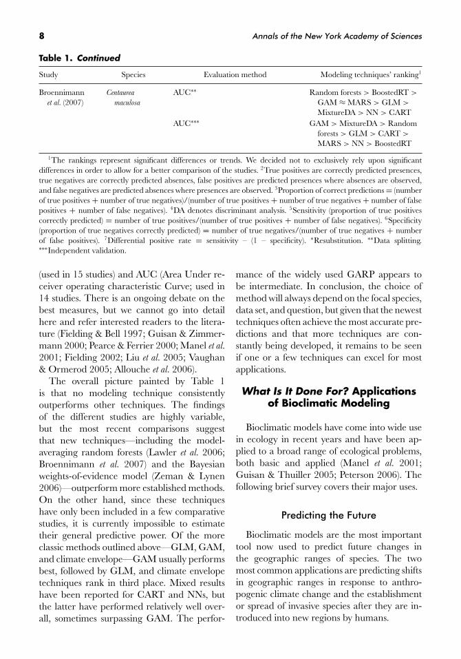
TABLE 1. Studies comparing the performance of different statistical methods

Study Species Evaluation method Modeling techniques’ ranking1

Studies that tested the models by means of resubstitution (cf. Fig. 1)Walker (1990) Kangaroos

(N = 3species)

False positives, false negatives2∗ CART > GLM

Skidmore et al.

(1996)Kangaroos

(N = 3)Proportion of correct predictions∗ CART > BIOCLIM > SNPC

Mastrorillo et al.

(1997)Fish (N = 3) Proportion of correct predictions3∗ NN > DA4

Bio et al. (1998) Plants(N = 156)

χ2∗ GAM > GLM

Franklin (1998) Plants(N = 20)

Residual deviance, false positives,false negatives∗

CART > GAM > GLM

Loiselle et al.

(2003)Birds (N = 11) Kappa∗ DOMAIN > Simple overlay >

GARP > GLM > BIOCLIMSegurado and

Araujo (2004)Amphibians,

reptiles(N = 44)

Sensitivity,5 kappa∗ NN > GAM > CART ≈ GLM >

Spatial interpolation >

BIOMAPPER ≈ DOMAINStudies that tested the models by means of data splittingManel et al. (1999) Birds (N = 6) Proportion of correct predictions∗ NN > DA > GLM

Proportion of correct predictions,sensitivity, specificity, kappa,among others∗∗

GLM > DA > NN

Vayssieres et al.

(2000)Oaks (N = 3) Sensitivity, specificity,6 differential

positive rate7∗∗CART > GLM

Elith andBurgman(2002)

Plants (N = 8) Area Under receiver operatingcharacteristic Curve (AUC)∗

GARP > GAM > GLM >

ANUCLIM

AUC∗∗ GAM > GLM > GARP >

ANUCLIMFertig and Reiners

(2002)Mentzelia

pumila

True positives, true negatives, falsepositives, false negatives∗,∗∗

CART ≈ GLM

Olden andJackson (2002)

Fish (N = 27),artificialspecies(N = 2)

Proportion of correct predictions,sensitivity, specificity∗∗

NN > CART ≈ DA ≈ GLM

Stockwell andPeterson (2002)

Birds(N = 103)

Proportion of correct predictions∗∗ GARP > GLM; performance ofcoarse and fine surrogate modelsheavily depend on sample size

Farber andKadmon (2003)

Woody plants(N = 192)

Proportion of correct predictions,sensitivity, specificity, kappa∗∗

Mahalanobis distance > BIOCLIM

Thuiller (2003) Trees (N = 61) AUC, kappa∗ NN > GAM > GLM > CARTAUC, kappa∗∗ NN > GAM > CART > GLM

Thuiller et al.

(2003)Trees (N = 4) AUC∗∗ GAM > GLM > CART

Continued


Table 1. Continued


Munoz andFelicısimo(2004)

Grimmia spp.,Fagus

sylvatica

AUC∗∗ CART ≈ MARS > GLM

Robertsonet al. (2004)

Plants (N = 3),cicadas(N = 3)

Kappa∗∗ FEM > BIOCLIM

Johnson andGillingham(2005)

Rangifer

tarandus

caribou

r, r s∗∗ Mahalanobis distance > GLM >

GARP > HSI

Elith et al.

(2006)Animals,

plants(N = 226)

AUC, correlation, kappa∗∗ BoostedRT ≈ MARS-COMM >

GDM ≈ Maxent > GAM >

GLM > DOMAIN ≈ GARP >

BIOCLIM ≈ LIVESHernandez

et al. (2006)Animals

(N = 18)AUC, sensitivity, area predicted

present, kappa∗∗Maxent > DOMAIN > GARP >

BIOCLIMLawler et al.

(2006)Mammals

(N = 100)AUC, sensitivity, specificity, kappa∗∗ Random forests > GLM >

GAM ≈ NN > CART ≈ GARPPearson et al.

(2006)Proteaceae

(N = 4)AUC, kappa∗∗ GAM ≈ NN > GLM >

DOMAIN > CART > GA >

GARP > BIOCLIMPhillips et al.

(2006)Mammals

(N = 2)Extrinsic omission rate,

proportional predicted area,AUC∗∗

Maxent > GARP

Randin et al.

(2006)Plants

(N = 54)AUC, kappa∗∗ GAM ≈ GLM

Schussmanet al. (2006)

Eragrostis

lehmanniana

Sensitivity, specificity, kappa∗∗ GLM > GARP

Zeman andLynen(2006)

Rhipicephalus

appendicula-

tus

Mean squared difference∗∗ Weights of evidence (Bayesian) >

GAM > DA

Meynard andQuinn(2007)

Artificialspecies(N = 18)

AUC, sensitivity, specificity, kappa,correlation true/predicted prob.of occurrence∗∗

GAM > GLM > CART > GARP

Peterson et al.

(2007)Birds (N = 3) AUC∗∗ Maxent > GARP

Tsoar et al.

(2007)Animals

(N = 42)Kappa∗∗ GARP > Mahalanobis distance >

HABITAT > DOMAIN >

BIOCLIM > ENFAStudies that tested the models by means of independent validationDettmers et al.

(2002)Birds (N = 6) Proportion of correct predictions∗∗ DA > CART > GLM >

Mahalanobis distanceProportion of correct predictions∗∗∗ CART > Mahalanobis distance >

GLM > DAAraujo et al.

(2005)Birds

(N = 116)AUC, kappa∗ NN > GAM ≈ GLM ≈ CART

AUC, kappa∗∗ NN > GAM ≈ GLM > CARTAUC, kappa∗∗∗ NN > GAM > GLM ≈ CART

Continued


Table 1. Continued


Broennimannet al. (2007)

Centaurea

maculosa

AUC∗∗ Random forests > BoostedRT >

GAM ≈ MARS > GLM >

MixtureDA > NN > CARTAUC∗∗∗ GAM > MixtureDA > Random

forests > GLM > CART >

MARS > NN > BoostedRT

1The rankings represent significant differences or trends. We decided not to exclusively rely upon significantdifferences in order to allow for a better comparison of the studies. 2True positives are correctly predicted presences,true negatives are correctly predicted absences, false positives are predicted presences where absences are observed,and false negatives are predicted absences where presences are observed. 3Proportion of correct predictions = (numberof true positives + number of true negatives)/(number of true positives + number of true negatives + number of falsepositives + number of false negatives). 4DA denotes discriminant analysis. 5Sensitivity (proportion of true positivescorrectly predicted) = number of true positives/(number of true positives + number of false negatives). 6Specificity(proportion of true negatives correctly predicted) = number of true negatives/(number of true negatives + numberof false positives). 7Differential positive rate = sensitivity – (1 – specificity). ∗Resubstitution. ∗∗Data splitting.∗∗∗Independent validation.

(used in 15 studies) and AUC (Area Under re-ceiver operating characteristic Curve; used in14 studies. There is an ongoing debate on thebest measures, but we cannot go into detailhere and refer interested readers to the litera-ture (Fielding & Bell 1997; Guisan & Zimmer-mann 2000; Pearce & Ferrier 2000; Manel et al.

2001; Fielding 2002; Liu et al. 2005; Vaughan& Ormerod 2005; Allouche et al. 2006).

The overall picture painted by Table 1is that no modeling technique consistentlyoutperforms other techniques. The findingsof the different studies are highly variable,but the most recent comparisons suggestthat new techniques—including the model-averaging random forests (Lawler et al. 2006;Broennimann et al. 2007) and the Bayesianweights-of-evidence model (Zeman & Lynen2006)—outperform more established methods.On the other hand, since these techniqueshave only been included in a few comparativestudies, it is currently impossible to estimatetheir general predictive power. Of the moreclassic methods outlined above—GLM, GAM,and climate envelope—GAM usually performsbest, followed by GLM, and climate envelopetechniques rank in third place. Mixed resultshave been reported for CART and NNs, butthe latter have performed relatively well over-all, sometimes surpassing GAM. The perfor-

mance of the widely used GARP appears tobe intermediate. In conclusion, the choice ofmethod will always depend on the focal species,data set, and question, but given that the newesttechniques often achieve the most accurate pre-dictions and that more techniques are con-stantly being developed, it remains to be seenif one or a few techniques can excel for mostapplications.

What Is It Done For? Applicationsof Bioclimatic Modeling

Bioclimatic models have come into wide usein ecology in recent years and have been ap-plied to a broad range of ecological problems,both basic and applied (Manel et al. 2001;Guisan & Thuiller 2005; Peterson 2006). Thefollowing brief survey covers their major uses.

Predicting the Future

Bioclimatic models are the most importanttool now used to predict future changes inthe geographic ranges of species. The twomost common applications are predicting shiftsin geographic ranges in response to anthro-pogenic climate change and the establishmentor spread of invasive species after they are in-troduced into new regions by humans.


Figure 1. Different strategies of model validation.(In color in Annals online.)

Predicting Responses to Climate ChangeBioclimatic models often are coupled to

climate-change models to predict how thegeographic ranges of species will shift asanthropogenic climate change proceeds (e.g.,Lindenmayer et al. 1991; Brereton et al. 1995;Oberhauser & Peterson 2003; Peterson et al.

2004a; Roura-Pascual et al. 2004; Araujo et al.

2005; Bomhard et al. 2005; Thuiller et al.

2005a,b; Walther et al. 2005; Tellez-Valdeset al. 2006; Lima et al. 2007; Nunes et al. 2007;Williams et al. 2007). The goal is typically to pre-dict the range (or survival) of species, but it mayalso be to compare the biological effects of dif-ferent climate-change scenarios. A wide rangeof species have been treated by these models,including economically or ecologically impor-

tant species such as crops, valuable speciesthat are harvested from the wild (e.g., timber,sport fishes), pests, diseases, biocontrol agents,foundation or keystone species, and imperiledspecies (Lindenmayer et al. 1991; Brereton et al.

1995; Roura-Pascual et al. 2004; Araujo et al.

2005; Bomhard et al. 2005; Parra-Oleaet al. 2005; Tellez-Valdes et al. 2006; Nuneset al. 2007).

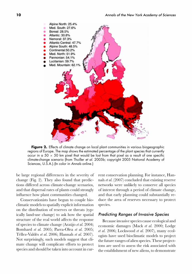
Thus, Thuiller et al. (2005b) used bio-climatic models to derive several importantinsights about how climate change might af-fect the local (i.e., a 50 × 50 km grid) com-position of plant communities in Europe. Theysuggested that climate change would cause bothlocal losses and gains of plant species, that thesechanges could be large, and that there would


Figure 2. Effects of climate change on local plant communities in various biogeographicregions of Europe. The map shows the estimated percentage of the plant species that currentlyoccur in a 50 × 50 km pixel that would be lost from that pixel as a result of one specificclimate-change scenario (from Thuiller et al. 2005b; copyright 2005 National Academy ofSciences, U.S.A.).(In color in Annals online.)

be large regional differences in the severity ofchange (Fig. 2). They also found that predic-tions differed across climate-change scenarios,and that dispersal rates of plants could stronglyinfluence how plant communities changed.

Conservationists have begun to couple bio-climatic models to spatially explicit informationon the distribution of reserves or threats (typ-ically land-use change) to ask how the spatialstructure of the real world affects the responseof species to climate change (Araujo et al. 2004;Bomhard et al. 2005; Parra-Olea et al. 2005;Tellez-Valdes et al. 2006; Hannah et al. 2007).Not surprisingly, such models suggest that cli-mate change will complicate efforts to protectspecies and should be taken into account in cur-

rent conservation planning. For instance, Han-nah et al. (2007) concluded that existing reservenetworks were unlikely to conserve all speciesof interest through a period of climate change,and that early planning could substantially re-duce the area of reserves necessary to protectspecies.

Predicting Ranges of Invasive Species

Because invasive species cause ecological andeconomic damages (Mack et al. 2000; Lodgeet al. 2006; Lockwood et al. 2007), many ecol-ogists have used bioclimatic models to projectthe future ranges of alien species. These project-ions are used to assess the risk associated withthe establishment of new aliens, to demonstrate


the need for import controls on potential pestspecies (Panetta & Mitchell 1991), or to targetmanagement actions to control these species(Peterson & Robins 2003). Bioclimatic modelsfor invasive species have been run for small re-gions (Iguchi et al. 2004, Underwood et al. 2004;Guo et al. 2005; Anderson et al. 2006), conti-nents (Strayer 1991; Sindel & Michael 1992;Beerling et al. 1995; Martin 1996; Petersonet al. 2003, 2004b, 2006a; Drake & Bossen-broek 2004; Drake & Lodge 2006; Zambranoet al. 2006; Chen et al. 2007; Fitzpatrick et al.

2007; Herborg et al. 2007; Loo et al. 2007),and the entire globe (Roura-Pascual et al. 2004;Ron 2005; Thuiller et al. 2005c; Li et al. 2006;Mohamed et al. 2006; Raimundo et al. 2007).Box 3 describes how the range of the inva-sive zebra mussel (Dreissena polymorpha) has beenpredicted in North America by means of bio-climatic modeling.

Figure 3 shows another example of the use ofa bioclimatic model to predict the range of aninvasive species in a new continent, and also il-lustrates the critical importance of careful eval-uation of model performance.Loo et al. (2007)used GARP to predict the potential range ofan invasive freshwater snail (Potamopyrgus antipo-

darum) in North America. Models based on itsnative distribution in New Zealand producedsatisfying fits for New Zealand (AUC = 0.73)but seriously underpredicted the range that thespecies has already achieved in North America.Models based on these existing North Ameri-can occurrences predicted a much wider po-tential range of this species in North Amer-ica. The large discrepancy between the twomodels has significant implications for themanagement and eventual impacts of thisspecies.

Bioclimatic models also have been used toassess whether the current range of a wellestablished alien is likely to increase in thefuture as it fills out its range (Martin 1996;Zambrano et al. 2006) or responds to anthro-pogenic climate change (Roura-Pascual et al.

2004). Herborg et al. (2007) combined the out-put from a bioclimatic model with estimates

of ballast water releases at various ports toidentify the entry points at which the Chi-nese mitten crab (Eriocheir sinensis) was mostlikely to invade, a problem with obvi-ous utility for monitoring and managementprograms.

Understanding the Present

Bioclimatic models also are widely used todescribe or interpret present-day species dis-tributions, or to address current managementproblems.

Investigating Mechanisms UnderlyingGeographic Ranges

Bioclimatic models have been used to investi-gate the roles of climate and other variables insetting the geographic ranges of species (Law1994; Manning et al. 2005; Rees et al. 2007).They may be run to see whether a particularvalue of a specific climatic variable hypothe-sized to be important in range bounding, or in-deed any climatic variable, coincides with theactual range boundary of a species. If the rangeboundary lines up with a climatic variable, thatvariable is interpreted as controlling the rangeboundary. If no climatic variable coincides withthe range boundary, then nonclimatic variablesare thought to be important. Ecologists havebeen particularly interested in whether climaticvariables or other causes are responsible for dis-junctions in species ranges, or whether large ar-eas of suitable climate exist that fail to supporta species for other reasons.

Describing the Actual Rangefrom Sparse Survey Data

The actual geographic range of a speciesmay be poorly known, especially if the speciesis cryptic in habit or has received little study.Bioclimatic models based on incomplete distri-butional information have been widely used toinfer the full geographic range of the species(Walther et al. 2004; Pearson et al. 2007; andreferences listed below). This exercise has manyapplications. The models can be used to guide


surveys for rare or valuable species in hithertounsampled areas (Lindenmayer et al. 1991;Villordon et al. 2006; Pearson et al. 2007). Es-timates of the actual range of a species can becompared to the distribution of protected ar-eas to assess whether the species is adequatelyprotected (Gaubert et al. 2006; Irfan-Ullah et al.

2007). Conservation assessments of rare speciestypically require information on the geographicrange of the species (IUCN 2007), which can beestimated by bioclimatic modeling (Sergio et al.

2007). Fine-scale estimates of actual ranges de-

rived from bioclimatic models have been usedas the basis of statistical analyses of the controlson species distributions or richness (White &Kerr 2007), or to identify areas of endemism(Escalante et al. 2007). Bioclimatic models haveeven been used to predict the geographic dis-tribution of diseases that are rare, such as Mar-burg hemorrhagic fever (Peterson et al. 2006b)and monkeypox (Levine et al. 2007), or forwhich the geographic range of vectors is poorlyknown (Peterson et al. 2004c; Adjemian et al.

2006).

BOX 3. A case study: predicting the range of the invasive zebra mussel (Dreissena polymorpha) in NorthAmerica.

– The appearance of the zebra mussel in North America in 1988 raised two critical questions: How badwill its impacts on freshwater ecosystems and infrastructure be? And how far will it spread? Bioclimaticmodels have been important in answering the latter question.

– Because zebra mussels are so widespread in Europe, even the earliest papers on its appearance in NorthAmerica (Hebert et al. 1989; Roberts 1990) noted that it might spread widely in North America. McMahonand Tsou (1990) made the first attempt to define its potential range more precisely. Applying results fromlaboratory studies on thermal tolerances of the species, they produced a rough map suggesting that thespecies might occupy a broad range from just north of the U.S.–Canada border to about the southerntier of states in the United States (see Figure for Box3). About the same time, Strayer (1991) developedformal bioclimatic models for the species based on its distribution in Europe and a suite of bioclimaticvariables. Although both the climatic variables (terrestrial climate variables collected from paper records)and the statistical analysis (discriminant analysis) would be considered primitive by modern standards,these models again showed the potential for zebra mussels to occupy a large range in North America.They also identified two key informational gaps. First, Strayer’s analysis suggested that the Europeanrange of the zebra mussel was not climate limited, so that any geographic ranges projected from itsEuropean distribution would have to be interpreted as minima (a caveat often overlooked by peoplewho cite this paper!). Second, although zebra mussel larvae require high levels of dissolved calcium tosurvive and develop, there were not good databases on environmental calcium concentrations that couldbe included in the models. It was clear that adding calcium to the models would severely reduce theprojected range of the species in North America.

– The next large advance in projecting the broad distribution of this species in North America did notcome until 2004, when Drake & Bossenbroek applied GARP models (based on the realized range ofzebra mussels in North America, rather than European records) to project the range of zebra musselsin North America. These models included more variables (climate, hydrology, geology) than Strayer’smodels, operated at a finer spatial scale, and produced much more detailed projections of the potentialNorth American range than earlier models. Nevertheless, Drake & Bossenbroek’s models still did notaddress calcium limitation very well. On the other hand, another recent model (Whittier et al. 2008)was based solely on environmental calcium concentrations, but did not include any climatic data, andproduced correspondingly different predictions for the range, especially in New England, the Southeast,and the Pacific Northwest.

– Any of these models is sufficient to identify the potential of zebra mussels to spread widely in NorthAmerica, and they are used widely by scientists and managers. The earliest models did not produce anyformal predictions for local occurrence of zebra mussels, and it remains to be seen how well the mostrecent models will meet the needs of managers to predict local details of the geographic range. It is


unfortunate that there has been very little rigorous comparison of models (but see Drake & Bossenbroek2004, for an illuminating exception), nor any effective combination of climate and calcium into a singlemodel. Finally, it is curious that the most recent models exclude Canada, which is after all where thespecies was first detected!

Figure for Box 3. Evolution of models to predict the geographic range of zebra mussels in NorthAmerica. Upper left: McMahon and Tsou’s (1990; copyright 1990 PennWell Corporation) model,based largely on thermal tolerances measured in the laboratory. Lower left: range limits from two ofStrayer’s (1991) projections, based on different thermal limits inferred by discriminant analysis fromthe European range of the species. Upper right: predictions from one of Drake and Bossenbroek’s(2004; copyright, American Institute of Biological Sciences) GARP models, based on the realizeddistribution of the species in North America. Darker shades show higher likelihood of invasion, anddots show localities from which the species was known as of 2003. Lower right: predictions fromWhittier et al. (2008; copyright 2008 Ecological Society of America), based on environmental calciumconcentrations. Dots show sites from which Dreissena spp. had been observed as of October 2007.(Incolor in Annals online.)

Identifying Suitable Sites for the Stockingor Culture of Valuable Species

Humans often deliberately move valuablespecies outside of their native range for agri-

culture, forestry, fisheries, or biological control.Bioclimatic models have been used to identifysuitable sites at which to stock or grow suchspecies, or to evaluate the reasons behind stock-ing failures (Richardson & McMahon 1992;


Figure 3. Potential range of the invasive freshwater snail Potamopyrgus antipodarum inNorth America based on (upper) its native range in New Zealand or (lower) its existing rangein North America (from Loo et al. 2007; copyright 2007 Ecological Society of America).Shading shows the proportion of best subset GARP models that predict the occurrence of thespecies, with darker shades showing areas where more models predict occurrence. Circlesshow known point occurrences of P. antipodarum in North America.

Cunningham et al. 2002). In a related applica-tion, scientists searching for suitable biocontrolagents for pest species or germplasm for cropshave used bioclimatic models to locate suitablesource areas which might be explored to findclimatically well adapted populations (Fiaboeet al. 2006; Villordon et al. 2006). It is inter-esting to note that scientists using bioclimaticmodels for these purposes sometimes observe

that a species can be established successfullyoutside its bioclimatic niche as defined fromits native range (e.g., Richardson & McMahon1992).

Clarifying Systematic Relationships

Finally, ecological information derived frombioclimatic models has been used to bolsterconclusions of taxonomic studies about the


distinctness of different populations that mightrepresent cryptic species (Fischer et al. 2001).The assumption here is that different specieswould have different climatic niches, so if twogroups of populations from different regions areshown to have different bioclimatic niches, theyare likely to be different species or subspecies.

Reconstructing the Past

Paleoecologists have long used biotic distri-butions to infer paleoclimates, either formallywith various models, or informally. Bioclimaticmodels have recently been used to assist inthese paleoclimatic inferences (Kershaw 1997;Kinzelbach et al. 1997; Dimitriadis & Cranston2001; Marra et al. 2004; van der Kaars et al.

2006; Ramstein et al. 2007). They have alsobeen used to reconstruct conditions in the re-cent past. For instance, it is difficult to know howmuch anthropogenic activities have reducedrange sizes for the many species whose historicranges are poorly known. In such cases, biocli-matic models can be used to reconstruct pastranges, against which current, known rangescan be compared to estimate range reductions(Bond et al. 2006). Alternatively, climatic datacan be combined with land-use data to esti-mate both past and present ranges to estimaterange reductions (Peterson et al. 2006c; Reeset al. 2007).

Does It Make Us Wiser? GeneralContributions of Bioclimatic

Modeling

Bioclimatic models have made several im-portant general contributions to ecology. Mostobviously, they have been a rich source of quan-titative projections or hypotheses concerningthe geographic ranges of species. These pro-jections or hypotheses are potentially of greatvalue in many areas of both basic and appliedecology, and are especially valuable becauseecologists have so few practical tools with whichto address these important questions. Because

Figure 4. The present-day range of the blacktufted-ear marmoset (Callithrix penicillata) as pre-dicted by the random forests model and compared tothe observed range (from Lawler et al. 2006; copy-right 2006 Lawler et al., Blackwell Publishing Ltd.).(Incolor in Annals online.)

of limited testing with respect to the variousapplications, however, the general usefulness ofbioclimatic models is currently unclear. We willcome back to this important point in the nextsection, Frontiers.

Bioclimatic models have shown consider-able abilities to fit even complicated geographicranges (Fig. 4), where the ranges of species withnarrow niches in climate space tend to be mod-eled more successfully than those with broaderniches (Kadmon et al. 2003; Tsoar et al. 2007).There has been some concern that bioclimaticmodels might perform poorly for species thathave very slow dispersal (Stockman et al. 2006)or are highly mobile (such species might be seenpassing through habitats that are not capableof supporting the species over the long term;Manning et al. 2005), but these issues have notbeen fully resolved.

The general ability of bioclimatic models tofit geographic ranges has reinforced the an-cient notion that climatic variables often ex-ert a primary control on the geographic ranges


of most species. This conclusion must be in-terpreted very cautiously, however, for severalreasons. First, species occur outside the rangespredicted by bioclimatic models (e.g., Richard-son & McMahon 1992; Loo et al. 2007), sug-gesting that nonclimatic factors are of primaryimportance in setting some range boundaries.Additionally, there have been few tests of biocli-matic models using freshwater or other poorlydispersing organisms for which dispersal ratherthan climate might be expected to set rangeboundaries. Further, the coincidence of a rangeboundary with an isoline of some climatic vari-able is not enough to demonstrate that theclimatic variable sets the range boundary, al-though it suggests a hypothesis that could betested by a more rigorous method. Finally, evenif the performance of bioclimatic models is in-terpreted as evidence that climate is impor-tant in setting geographic ranges, the consid-erable variation in species distributions thatis not explained by these models shows thatthere is ample room for other factors (biolog-ical interactions, dispersal) to be important aswell.

Bioclimatic models have made essential con-tributions to the scientific and public discussionabout the ecological effects of anthropogenicclimate change by providing quantitative sce-narios and visualizations (e.g., Fig. 2). Even ifthese scenarios cannot always be regarded asliteral predictions of the future, they certainlyshow that climate change is likely to cause largeshifts in biotic distributions, that climate changewill interact strongly with other anthropogenicdrivers such as land-use change (Araujo et al.

2004; Bomhard et al. 2005; Parra-Olea et al.

2005; Tellez-Valdes et al. 2006; Hannahet al. 2007), and that conservation planning andreserve design will need to take climate changeinto account (e.g., Hannah et al. 2007). Anotherapplied issue addressed by bioclimatic models isthe pressing problem of invasive species, includ-ing diseases. Bioclimatic models have shownthat most invasive species have considerableunrealized potential to spread (along with theirecological and economic impacts) (e.g., Fig. 3and references cited above), as long as humans

continue to be careless about providing thesespecies with transport opportunities. Finally,bioclimatic models have been helpful in conser-vation planning and surveys for rare species byproviding estimates of actual geographic rangesfrom sparse survey data. Although it might beargued that we didn’t need a model to tell usthat anthropogenic climate change would af-fect species ranges or that invasive species poseecological and economic threats, the quanti-tative output and powerfully evocative mapsproduced by bioclimatic models (Figs. 2 and 3)have lent weight and urgency to discussions ofthese issues.

Finally, bioclimatic modeling has broughta number of sophisticated statistical model-ing techniques to ecology (see section Statistical

Methods). Methods used for bioclimatic model-ing have obvious utility for habitat modelingin general, as well as other ecological appli-cations. Further, the increasingly sophisticateddiscussion about evaluating the performanceof bioclimatic models (Fielding & Bell 1997;Guisan & Zimmermann 2000; Pearce & Ferrier2000; Manel et al. 2001; Fielding 2002; Liuet al. 2005; Vaughan & Ormerod 2005; Al-louche et al. 2006) has the potential to sub-stantially improve the interpretation of modelswith binary output, which are widely used inecology.

What Are the Major Obstaclesand Needs? Frontiers

Bioclimatic Models Are OftenApplied but Rarely Tested

The testing and evaluation of bioclimaticmodels need to be tied more closely to theirspecific intended uses. Two issues deserve morecareful attention: the degree of fit between themodel and the test data, and the type of datathat are used to evaluate the model. Many stud-ies have judged model performance using weakcriteria (e.g., simply whether the model per-forms better than random) that do not showhow useful the model will be for a particularapplication. The metric used to judge a model


(e.g., AUC, Cohen’s kappa, true skill statistic,sensitivity, specificity) and the value of that met-ric needed to demonstrate that a model is usefulboth depend entirely on the intended uses of themodel. Just as there is no special value of r2 thatshows that a linear regression is adequate, therewill be no single value of AUC or kappa thatshows that a bioclimatic model is adequate forall purposes.

The appropriate data for testing a modellikewise depend on the intended use of themodel (Fig. 1). If a bioclimatic model is intendedto identify a species’ present-day range basedon sparse survey data (see section What is it done

for?), it may be sufficient to evaluate model per-formance by splitting the data into a training setused to fit the model and a validation set used toevaluate the model. Such tests have been donefrequently. Thus, studies given in Table 1 thatapplied this evaluation method reported an av-erage value of 0.85 ± 0.029 (SE; N = 12) forAUC, where a random predictor has a value of0.5, a perfect predictor achieves 1, and a value≥0.9 is usually taken to indicate high accuracy(Swets 1988; Manel et al. 2001; Araujo et al.

2005; Pearson et al. 2006; Randin et al. 2006).For kappa, the average value of studies listedin Table 1 is 0.52 ± 0.065 (SE; N = 12); here,a random predictor has a value of 0, a perfectpredictor achieves 1, and the benchmark forhigh accuracy is 0.7–0.75 (Monserud & Lee-mans 1992; Fielding & Bell 1997; Araujo et al.

2005; Pearson et al. 2006; Randin et al. 2006).While in a general sense these metrics suggestthat bioclimatic models of present-day rangesperform satisfactorily, only an individual modeluser can really say whether these values of AUCor kappa are high enough (or indeed, whetherAUC or kappa are the appropriate metrics).

For most applications of bioclimatic model-ing, especially for predicting range shifts dueto climate change or the spread of invaders,model performance should be tested by meansof independent validation, rather than resub-stitution or data splitting (cf. Fig. 1). It is usuallydifficult to locate such independent data sets, sostudies that apply this method are currently the

exception (Box 4). A number of paleoecologicalstudies evaluated bioclimatic models based oninferred past climatic conditions (Prentice et al.

1991; Martınez-Meyer et al. 2004; Martınez-Meyer & Peterson 2006; Ramstein et al. 2007).This is the best one can do if past climaticconditions are unknown, but we do not listsuch model evaluations in Box 4, as they areless reliable and not directly comparable toevaluations based on measured climate data.Most of the studies in Box 4 only evaluatedthe models against random predictions or didnot calculate any objective evaluation mea-sure. Only a few calculated gradual quantita-tive evaluation measures: Araujo et al. (2005),Lima et al. (2007), Loo et al. (2007), and Broen-nimann et al. (2007) reported AUC values of0.80, 0.73, 0.61, and 0.50 on average, respec-tively; Walther et al. (2005) and Araujo et al.

(2005) reported kappa values of 0.50 and 0.42,respectively; and Dettmers et al. (2002) reportedan average proportion of correct predictions of0.55. As expected, these metrics suggest thatbioclimatic models perform less successfullywhen training data and test data are spatially ortemporally independent than if both are fromthe same region and time. But again, whetherthese metrics indicate satisfactory model per-formance depends on the needs of the modeluser.

BOX 4. Studies that tested bioclimatic modelsby means of independent validation (cf. Fig. 1)

– Predicting the futureClimate change: Araujo et al. (2005), Walther et al.

(2005), Lima et al. (2007), Nunes et al. (2007)Invaders: Beerling et al. (1995), Peterson and

Vieglais (2001), Peterson et al. (2003),Thuiller et al. (2005c), Broennimann et al.

(2007), Fitzpatrick et al. (2007), Loo et al.

(2007)– Understanding the present: Dettmers et al.

(2002)– Reconstructing the past: Kinzelbach et al.

(1997), Hill et al. (1999).


Extending Bioclimatic Models

In spite of the scarcity of information, wemay cautiously conclude from the last sec-tion that bioclimatic models, especially for pro-jecting range shifts due to climate change orthe spread of invaders, need further improve-ment before they reliably lead to excellent oreven good predictions. An important step to-wards this goal may be taken by consideringthe above-mentioned key assumptions of bio-climatic models (section How is it done?). Somestudies already extended the current model-ing approach by considering species interac-tions (Leathwick & Austin 2001; Anderson et al.

2002; Leathwick 2002; Araujo & Luoto 2007;Heikkinen et al. 2007; Sutherst et al. 2007). Dis-persal limitation has sometimes been includedby an assumed maximum dispersal distance(Midgley et al. 2006; Williams et al. 2007) or bysimply assuming that climatically suitable areasthat lie beyond obstacles such as mountains arenot within the potential range of the species(Peterson et al. 2006c; Irfan-Ullah et al. 2007);only a few studies applied more complex disper-sal models (Carey 1996; Iverson et al. 2004). Itwould be important to continue this work on ex-tended bioclimatic models and then rigorouslytest the models by means of independent valida-tion, also in comparison to ordinary bioclimaticmodels in order to learn how much is gainedby considering species interactions or dispersallimitation. The limited knowledge we have sofar suggests that the gain can be substantial.

Acknowledgments

We thank Astrid van Teeffelen and JackWilliams for discussion, two anonymous re-viewers for helpful comments, and Thom Whit-tier for supplying a copy of his figure. TheDeutsche Forschungsgemeinschaft (JE 288/2-1) and National Science Foundation (DEB0235385) provided financial support.

Conflicts of Interest

The authors declare no conflicts of interest.

References

Adjemian, J.C.Z. et al. 2006. Analysis of Genetic Algo-rithm for Rule-Set Production (GARP) modeling ap-proach for predicting distributions of fleas implicatedas vectors of plague, Yersinia pestis, in California. J.

Med. Entomol. 43: 93–103.Allouche, O., A. Tsoar & R. Kadmon. 2006. Assessing the

accuracy of species distribution models: prevalence,kappa and the true skill statistic (TSS). J. Appl. Ecol.

43: 1223–1232.Anderson, R.P., A.T. Peterson & M. Gomez-Laverde.

2002. Using niche-based GIS modeling to test ge-ographic predictions of competitive exclusion andcompetitive release in South American pocket mice.Oikos 98: 3–16.

Anderson, R.P., A.T. Peterson & S.L. Egbert. 2006.Vegetation-index models predict areas vulnerableto purple loosestrife (Lythrum salicaria) invasion inKansas. Southwest. Nat. 51: 471–480.

Araujo, M.B. & M. Luoto. 2007. The importance of bioticinteractions for modelling species distributions underclimate change. Global Ecol. Biogeogr. 16: 743–753.

Araujo, M.B. et al. 2004. Would climate change drivespecies out of reserves? An assessment of existingreserve-selection methods. Global Change Biol. 10:1618–1626.

Araujo, M.B. et al. 2005. Validation of species-climateimpact models under climate change. Global Change

Biol. 11: 1504–1513.Beerling, D.J., B. Huntley & J.P. Bailey. 1995. Climate

and the distribution of Fallopia japonica: use of anintroduced species to test the predictive capac-ity of response surfaces. J. Vegetation Sci. 6: 269–282.

Begon, M., C.R. Townsend & J.L. Harper. 2005. Ecol-

ogy: Individuals, Populations and Communities, 4th edn.Blackwell. Oxford.

Bio, A.M.F., R. Alkemande & A. Barendregt. 1998. De-termining alternative models for vegetation responseanalysis – a non-parametric approach. J. Vegetation

Sci. 9: 5–16.Blackburn, T.M. & K.J. Gaston, Eds. 2003. Macroecology:

Concepts and Consequences. Blackwell. Oxford.Blossey, B., & R. Notzold. 1995. Evolution of increased

competitive ability in invasive nonindigenous plants:A hypothesis. J. Ecol. 83: 887–889.

Bomhard, B. et al. 2005. Potential impacts of future landuse and climate change on the Red List status ofthe Proteaceae in the Cape Floristic Region, SouthAfrica. Global Change Biol. 11: 1452–1468.

Bond, J.E. et al. 2006. Combining genetic and geospatialanalyses to infer population extinction in mygalo-morph spiders endemic to the Los Angeles region.Anim. Conserv. 9: 145–157.


Breiman, L. et al. 1984. Classification and Regression Trees.Chapman & Hall. New York.

Brereton, R., S. Bennett & I. Mansergh. 1995. Enhancedgreenhouse climate change and its potential effect onselected fauna of south-eastern Australia – a trendanalysis. Biol. Conserv. 72: 339–354.

Broennimann, O. et al. 2007. Evidence of climatic nicheshift during biological invasion. Ecol. Lett. 10: 701–709.

Brown, J.H. & Maurer, B.A. 1989. Macroecology: thedivision of food and space among species on conti-nents. Science 243: 1145–1150.

Brown, J.H. 1995. Macroecology. University of ChicagoPress. Chicago, Illinois.

Brown, J.H., G.C. Stevens & D.M. Kaufman. 1996.The geographic range: size, shape, boundaries, andinternal structure. Annu. Rev. Ecol. Syst. 27: 597–623.

Carey, P.D. 1996. DISPERSE: A cellular automaton forpredicting the distribution of species in a changedclimate. Global Ecol. Biogeogr. Lett. 5: 217–226.

Chen, P.F., E.O. Wiley & K.M. McNyset. 2007. Ecolog-ical niche modeling as a predictive tool: silver andbighead carps in North America. Biol. Invasions 9:43–51.

Cox, G.W. 2004. Alien Species and Evolution: The Evolutionary

Ecology of Exotic Plants, Animals, Microbes, and Interacting

Native Species. Island Press. Washington, DC.Cunningham, D.C., E.R. Anderson & K.B. Walsh. 2002.

Ecology and biogeography of Cassia brewsteri: assess-ment of potential sites for cultivation. Aust. J. Exp.

Agr. 42: 1071–1080.Daehler, C.C. 2003. Performance comparisons of co-

occuring native and alien invasive plants: implica-tions for conservation and restoration. Annu. Rev. Ecol.

Syst. 34: 183–211.Davis, A.J. et al. 1998a. Individualistic species responses

invalidate simple physiological models of commu-nity dynamics under global environmental change.J. Anim. Ecol. 67: 600–612.

Davis, A.J. et al. 1998b. Making mistakes when predictingshifts in species range in response to global warming.Nature 391: 783–786.

Davis, M.B. & R.G. Shaw. 2001. Range shifts and adap-tive responses to Quaternary climate change. Science

292: 673–679.Dettmers, R., D.A. Buehler & J.B. Bartlett. 2002. A test

and comparison of wildlife-habitat modeling tech-niques for predicting bird occurrence at a regionalscale. In Predicting Species Occurrences: Issues of Accuracy

and Scale. J.M. Scott et al., Eds.: 607–615. Island Press.Washington, DC.

DeWitt, T.J. & S.M. Scheiner, Eds. 2004. Phenotypic plas-

ticity: Functional and Conceptual Approaches. Oxford Uni-versity Press. New York.

Dimitriadis, S. & P.S. Cranston. 2001. An AustralianHolocene climate reconstruction using Chironomi-dae from a tropical volcanic maar lake. Palaeogeogr.

Palaeoecol. 176: 109–131.Doley, D. 1977. Parthenium weed (Parthenium hysterophorus

L.): gas exchange characteristics as a basis for pre-diction of its geographical distribution. Aust. J. Agric.

Res. 28: 449–460.Drake, J.M. & J.M. Bossenbroek. 2004. The potential

distribution of zebra mussels in the United States.BioScience 54: 931–941.

Drake, J.M. & D.M. Lodge. 2006. Forecasting potentialdistributions of nonindigenous species with a geneticalgorithm. Fisheries 31: 9–16.

Elith, J. & M. Burgman. 2002. Predictions and their val-idation: rare plants in the Central Highlands, Vic-toria, Australia. In Predicting Species Occurrences: Issues

of Accuracy and Scale. J.M. Scott et al., Eds.: 303–313.Island Press. Washington, DC.

Elith, J. et al. 2006. Novel methods improve prediction ofspecies’ distributions from occurrence data. Ecography

29: 129–151.Escalante, T. et al. 2007. Areas of endemism of Mexi-

can terrestrial mammals: a case study using species’ecological niche modeling, parsimony analysis ofendemicity and Goloboff fit. Interciencia 32: 151–159.

Farber, O. & R. Kadmon. 2003. Assessment of alterna-tive approaches for bioclimatic modeling with specialemphasis on the Mahalanobis distance. Ecol. Model.

160: 115–130.Fertig, W. & W.A. Reiners. 2002. Predicting pres-

ence/absence of plant species for range mapping:a case study from Wyoming. In Predicting Species Oc-

currences: Issues of Accuracy and Scale. J.M. Scott et al.,Eds.: 483–489. Island Press. Washington, DC.

Fiaboe, K.K.M. et al. 2006. Identification of priority ar-eas in South America for classical biological controlof Tetranychus evansi (Acari: Tetranychidae) in Africa.Biol. Control 38: 373–379.

Fielding, A.H. 2002. What are the appropriate charac-teristics of an accuracy measurement? In Predicting

Species Occurrences: Issues of Accuracy and Scale. J.M. Scottet al., Eds.: 271–280. Island Press. Washington, DC.

Fielding, A.H. & J.F. Bell. 1997. A review of methods forthe assessment of prediction errors in conservationpresence/absence models. Environ. Conserv. 24: 38–49.

Fischer, J. et al. 2001. Climate and animal distribution:a climatic analysis of the Australian marsupial Tri-

chosurus caninus. J. Biogeogr. 28: 293–304.Fitzpatrick, M.C. et al. 2007. The biogeography of predic-

tion error: why does the introduced range of the fireant over-predict its native range? Global Ecol. Biogeogr.

16: 24–33.


Franklin, J. 1998. Predicting the distribution of shrubspecies in southern California from climate andterrain-derived variables. J. Vegetation Sci. 9: 733–748.

Gaston, K.J. 2003. The Structure and Dynamics of Geographic

Ranges. Oxford University Press. Oxford.Gaubert, P., M. Papes & A.T. Peterson. 2006. Natural

history collections and the conservation of poorlyknown taxa: ecological niche modeling in centralAfrican rainforest genets (Genetta spp.). Biol. Conserv.

130: 106–117.Guisan, A. & N.E. Zimmermann. 2000. Predictive habi-

tat distribution models in ecology. Ecol. Model. 135:147–186.

Guisan, A. & W. Thuiller. 2005. Predicting species dis-tribution: offering more than simple habitat models.Ecol. Lett. 8: 993–1009.

Guo, Q., M. Kelly & C.H. Graham. 2005. Support vectormachines for predicting distribution of Sudden OakDeath in California. Ecol. Model. 182: 75–90.

Hampe, A. 2004. Bioclimate envelope models: what theydetect and what they hide. Global Ecol. Biogeogr. 12:469–471.

Hannah, L. et al. 2007. Protected area needs in a changingclimate. Front. Ecol. Environ. 5: 131–138.

Hanski, I. 1999. Metapopulation Ecology. Oxford UniversityPress. Oxford.

Hastie, T.J. & R.J. Tibshirani. 1990. Generalized Additive

Models. Chapman & Hall/CRC. Boca Raton.Hebert, P.D.N. et al. 1989. Ecological and genetic studies

on Dreissena polymorpha (Pallas): a new mollusc in theGreat Lakes. Can. J. Fish. Aquat. Sci. 46: 1587–1591.

Heikkinen, R.K. et al. 2006. Methods and uncertain-ties in bioclimatic envelope modelling under climatechange. Prog. Phys. Geog. 30: 751–777.

Heikkinen, R.K. et al. 2007. Biotic interactions improveprediction of boreal bird distributions at macro-scales. Global Ecol. Biogeogr. 16: 754–763.

Herborg, L.-M. et al. 2007. Predicting invasion risk usingmeasures of introduction effort and environmentalniche models. Ecol. Appl. 17: 663–674.

Hernandez, P.A. et al. 2006. The effect of sample size andspecies characteristics on performance of differentspecies distribution modeling methods. Ecography 29:773–785.

Hill, J.K., C.D. Thomas & B. Huntley. 1999. Climate andhabitat availability determine 20th century changesin a butterfly’s range margin. Proc. R. Soc. Lond. B

266: 1197–1206.Hijmans, R.J. & C.H. Graham. 2006. The ability of cli-

mate envelope models to predict the effect of climatechange on species distributions. Global Change Biol.

12: 2272–2281.Hosmer, D.W. & S. Lemeshow. 2000. Applied Logistic Re-

gression, 2nd edn. Wiley. New York.Huntley, B. 1995. Plant-species response to climate

change—implications for the conservation of Euro-pean birds. Ibis 137: S127—S138.

Hutchinson, G.E. 1957. Concluding remarks. Cold Spr.

Harb. Symp. Quant. Biol. 22: 415–427.Iguchi, K. et al. 2004. Predicting invasions of North Amer-

ican basses in Japan using native range data and agenetic algorithm. T. Am. Fish. Soc. 133: 845–854.

Irfan-Ullah, M. et al. 2007. Mapping the geographic dis-tribution of Aglaia bourdillonii Gamble (Meliaceae),an endemic and threatened plant, using ecologicalniche modeling. Biodiv. Conserv. 16: 1917–1925.

IUCN. 2007. 2007 IUCN Red List of ThreatenedSpecies. http://www.iucnredlist.org.

Iverson, L.R., M.W. Schwartz & A.M. Prasad. 2004. Howfast and far might tree species migrate in the easternUnited States due to climate change? Global Ecol.Biogeogr. 13: 209–219.

Johnson, C.J. & M.P. Gillingham. 2005. An evaluation ofmapped species distribution models used for conser-vation planning. Environ. Conserv. 32: 117–128.

Kadmon, R., O. Farber & A. Danin. 2003. A system-atic analysis of factors affecting the performance ofclimatic envelope models. Ecol. Appl. 13: 853–867.

Karban, R. & I.T. Baldwin. 1997. Induced Responses to Her-

bivory. University of Chicago Press. Chicago, Illinois.Keane, R.M. & M.J. Crawley. 2002. Exotic plant inva-

sions and the enemy release hypothesis. Trends Ecol.

Evol. 17: 164–170.Kearney, M. & W.P. Porter. 2004. Mapping the funda-

mental niche: physiology, climate, and the distribu-tion of a nocturnal lizard. Ecology 85: 3119–3131.

Kershaw, A.P. 1997. A bioclimatic analysis of early tomiddle Miocene brown coal floras, Latrobe Valley,south-eastern Australia. Aust. J. Bot. 45: 373–387.

Kinzelbach, R., B. Nicolai & R. Schlenker. 1997. DerBienenfresser Merops apiaster als Klimaanzeiger: ZumEinflug in Bayern, der Schweiz und Baden im Jahr1644. J. Ornithol. 138: 297–308.

Law, B.S. 1994. Climatic limitation of the southern distri-bution of the common blossom bat Syconycteris australis

in New South Wales. Aust. J. Ecol. 19: 366–374.Lawler, J.J. et al. 2006. Predicting climate-induced range

shifts: model differences and model reliability. Global

Change Biol. 12: 1568–1584.Lawton, J.H. 2001. Biodiversity, ecosystem processes and

climate change. In Ecology: Achievement and Challenge.M.C. Press, N.J. Huntly & S. Levin, Eds.: 139–160.Blackwell. Oxford.

Leathwick, J.R. & M.P. Austin. 2001. Competitive in-teractions between tree species in New Zealand’sold-growth indigenous forests. Ecology 82: 2560–2573.

Leathwick, J.R. 2002. Intra-generic competition amongNothofagus in New Zealand’s primary indigenousforests. Biodivers. Conserv. 11: 2177–2187.


Levine, R.S. et al. 2007. Ecological niche and geographicdistribution of human monkeypox in Africa. PLoS

ONE 2: e176.Li, H. et al. 2006. Potential global range expansion of

a new invasive species, the erythrina gall wasp,Quadrastichus erythrinae Kim (Insecta: Hymenoptera:Eulophidae). Raffles B. Zool. 54: 229–234.

Lima, F. et al. 2007. Modelling past and present geographi-cal distribution of the marine gastropod Patella rustica

as a tool for exploring responses to environmentalchange. Global Change Biol. 13: 2065–2077.

Lindenmayer, D.B. et al. 1991. The conservation of Lead-beater’s possum, Gymnobelideus leadbeateri (McCoy) –a case study of the use of bioclimatic modeling. J.

Biogeogr. 18: 371–383.Liu, C. et al. 2005. Selecting thresholds of occurrence in

the prediction of species distributions. Ecography 28:385–393.

Lockwood, J.L., M.F. Hoopes & M.P. Marchetti. 2007.Invasion Ecology. Blackwell. Malden, Massachusetts.

Lodge, D.M. et al. 2006. Biological invasions: recommen-dations for U.S. policy and management. Ecol. Appl.

16: 2035–2054.Loiselle, B.A. et al. 2003. Avoiding pitfalls of using species

distribution models in conservation planning. Conserv.

Biol. 17: 1591–1600.Loo, S.E., R. Mac Nally & P.S. Lake. 2007. Forecasting

New Zealand mudsnail invasion range: model com-parisons using native and invaded ranges. Ecol. Appl.

17: 181–189.Mack, R.N. et al. 2000. Biotic invasions: causes, epidemi-

ology, global consequences, and control. Ecol. Appl.

10: 689–710.Manel, S. et al. 1999. Alternative methods for predicting

species distribution: an illustration with Himalayanriver birds. J. Appl. Ecol. 36: 734–747.

Manel, S., H.C. Williams & S.J. Ormerod. 2001. Evalu-ating presence-absence models in ecology: the needto account for prevalence. J. Appl. Ecol. 38: 921–931.

Manning, A.D. et al. 2005. A bioclimatic analysis for thehighly mobile Superb Parrot of south-eastern Aus-tralia. Emu 105: 193–201.

Marra, M.J. et al. 2004. Late Quaternary climate changein the Awatere valley, South Island, New Zealand,using a sine model with a maximum likelihoodenvelope on fossil beetle data. Quaternary Sci. Rev. 23:1637–1650.

Martin, W.K. 1996. The current and potential distribu-tion of the common myna Acridotheres tristis in Aus-tralia. Emu 96: 166–173.

Martınez-Meyer, E. & A.T. Peterson. 2006. Conservatismof ecological niche characteristics in North Americanplant species over the Pleistocene-to-Recent transi-tion. J. Biogeogr. 33: 1779–1789.

Martınez-Meyer, E., A.T. Peterson & W.W. Hargroves.2004. Ecological niches as stable distributionalconstraints on mammal species, with implicationsfor Pleistocene extinctions and climate projectionsfor biodiversity. Global Ecol. Biogeogr. 13: 305–314.

Mastrorillo, S. et al. 1997. The use of artificial neuralnetworks to predict the presence of small-bodied fishin a river. Freshw. Biol. 38: 237–246.

McMahon, R.F. & J.L. Tsou. 1990. Impact of Europeanzebra mussel infestation to the electric power indus-try. Prof. Am. Power Conf. 52: 988–997.

Meynard, C.N. & J.F. Quinn. 2007. Predicting species dis-tributions: a critical comparison of the most commonstatistical models using artificial species. J. Biogeogr.

34: 1455–1469.Midgley, G.F. et al. 2006. Migration rate limitations on

climate change-induced range shifts in Cape Pro-teaceae. Diversity Distrib. 12: 555–562.

Mitchell, C.E. & A.G. Power. 2003. Release of invasiveplants from fungal and viral pathogens. Nature 421:625–627.

Mohamed, K.I. et al. 2006. Global invasive potential of10 parasitic witchweeds and related Orobanchaceae.Ambio 35: 281–288.

Monserud, R.A. & R. Leemans. 1992. Comparing globalvegetation maps with the Kappa statistic. Ecol. Model.

62: 275–293.Munoz, J. & A.M. Felicısimo. 2004. Comparison of sta-

tistical methods commonly used in predictive mod-elling. J. Vegetation Sci. 15: 285–292.

Nunes, M.F.C. et al. 2007. Are large-scaled distributionalshifts of the blue-winged macaw (Primolus maracana)related to climate change? J. Biogeogr. 34: 816–827.

Oberhauser, K. & A.T. Peterson. 2003. Modeling currentand future potential wintering distributions of east-ern North American monarch butterflies. Proc. Natl.

Acad. Sci. USA 100: 14063–14068.Olden, J.D. & D.A. Jackson. 2002. A comparison of statis-

tical approaches for modelling fish species distribu-tions. Freshw. Biol. 47: 1976–1995.

Panetta, F.D. & N.D. Mitchell. 1991. Bioclimatic pre-diction of the potential distributions of some weedspecies prohibited entry into New Zealand. N. Z. J.

Agr. Res. 34: 341–350.Parra-Olea, G., E. Martınez-Meyer & G.F.P. de Leon.

2005. Forecasting climate change effects on salaman-der distribution in the highlands of central Mexico.Biotropica 37: 202–208.

Patterson, D.T. et al. 1979. Temperature responses and po-tential distribution of itchgrass (Rottboellia exaltata)in the United States. Weed Sci. 27: 77–82.

Pearce, J. & S. Ferrier. 2000. Evaluating the predictive per-formance of habitat models developed using logisticregression. Ecol. Model. 133: 225–245.


Pearson, R.G. 2006. Climate change and the migra-tion capacity of species. Trends Ecol. Evol. 21: 111–113.

Pearson, R.G. & T.P. Dawson. 2003. Predicting the im-pacts of climate change on the distribution of species:are bioclimate envelope models useful? Global Ecol.Biogeogr. 12: 361–371.

Pearson, R.G. et al. 2006. Model-based uncertainty inspecies range prediction. J. Biogeogr. 33: 1704–1711.

Pearson, R.G. et al. 2007. Predicting species distributionsfrom small numbers of occurrence records: a testcase using cryptic geckos in Madagascar. J. Biogeogr.

34: 102–117.Peterson, A.T. 2001. Predicting species’ geographic distri-

butions based on ecological niche modeling. Condor

103: 599–605.Peterson, A.T. 2003. Predicting the geography of species’

invasions via ecological niche modeling. Q. Rev. Biol.

78: 419–433.Peterson, A.T. 2006. Uses and requirements of ecologi-

cal niche models and related distributional models.Biodiv. Inform. 3: 59–72.

Peterson, A.T. & C.R. Robins. 2003. Using ecological-niche modeling to predict barred owl invasions withimplications for spotted owl conservation. Conserv.

Biol. 17: 1161–1165.Peterson, A.T. & D.A. Vieglais. 2001. Predicting species

invasions using ecological niche modeling: new ap-proaches from bioinformatics attack a pressing prob-lem. BioScience 51: 363–371.

Peterson, A.T., M. Papes & D.A. Kluza. 2003. Predictingthe potential invasive distributions of four alien plantspecies in North America. Weed Sci. 51: 863–868.

Peterson, A.T. et al. 2004a. Modeled climate change effectsof distributions of Canadian butterfly species. Can. J.

Zool. 82: 851–858.Peterson, A.T., R. Scachetti-Pereira & W.W. Har-

grove. 2004b. Potential geographic distribution ofAnoplophora glabripennis (Coleoptera: Cerambycidae)in North America. Am. Midl. Nat. 151: 170–178.

Peterson, A.T., R. Scachetti-Pereira & V.F. de CamargoNeves. 2004c. Using epidemiological survey data toinfer geographic distributions of leishmaniasis vectorspecies. Rev. Soc. Bras. Med. Tro. 37: 10–14.

Peterson A.T. et al. 2006a. Native-range ecology and in-vasive potential of Cricetomys in North America. J.

Mammal. 87: 427–432.Peterson, A.T. et al. 2006b. Geographic potential for out-

breaks of Marburg hemorrhagic fever. Am. J. Trop.

Med. Hyg. 75: 9–15.Peterson, A.T. et al. 2006c. Tracking population ex-

tirpations via melding ecological niche modelingwith land-cover information. Ecol. Model. 195: 229–236.

Peterson, A.T., M. Papes & M. Eaton. 2007. Transferabil-ity and model evaluation in ecological niche model-ing: A comparison of GARP and Maxent. Ecography

30: 550–560.Phillips, S.J., R.P. Anderson & R.E. Schapire. 2006. Max-

imum entropy modeling of species geographic distri-butions. Ecol. Model. 190: 231–259.

Prentice, I.C., P.J. Bartlein & T. Webb III. 1991. Vegeta-tion and climate change in eastern North Americasince the last glacial maximum. Ecology 72: 2038–2056.

Prentice, I.C. et al. 1992. A global biome model based onplant physiology and dominance, soil properties andclimate. J. Biogeogr. 19: 117–134.

Raimundo, R.L.G. et al. 2007. Native and exotic distribu-tions of siamweed (Chromolaena odorata) modeled usingthe genetic algorithm for rule-set production. Weed

Sci. 55: 41–48.Ramstein, G. et al. 2007. How cold was Europe at the

Last Glacial Maximum? A synthesis of the progressachieved since the first PMIP model-data compari-son. Clim. Past 3: 331–339.

Randin, C.F. et al. 2006. Are niche-based species distri-bution models transferable in space? J. Biogeogr. 33:1689–1703.

Rees, M., D.J. Paull & S.M. Carthew. 2007. Factors in-fluencing the distribution of the yellow-bellied glider(Petaurus australis australis) in Victoria, Australia. Wildl.

Res. 34: 228–233.Richardson, D.M. & J.P. McMahon. 1992. A bioclimatic

analysis of Eucalyptus nitens to identify potential plant-ing regions in southern Africa. S. Afr. J. Sci. 88: 380–387.

Roberts, L. 1990. Zebra mussel invasion threatens U.S.waters. Science 249: 1370–1372.

Robertson, M.P., M.H. Villet & A.R. Palmer. 2004. Afuzzy classification technique for predicting species’distributions: applications using invasive alien plantsand indigenous insects. Diversity Distrib. 10: 461–474.

Ron, S.R. 2005. Predicting the distribution of the am-phibian pathogen Batrachochytrium dendrobatidis in theNew World. Biotropica 37: 209–221.

Roura-Pascual, N. et al. 2004. Geographical potential ofArgentine ants (Linepithema humile Mayr) in the faceof global climate change. Proc. R. Soc. B 271: 2527–2534.

Sax, D.F. et al. 2007. Ecological and evolutionary insightsfrom species invasions. Trends Ecol. Evol. 22: 465–471.

Schmitz, O.J. et al. 2003. Ecosystem responses to globalclimate change: Moving beyond color mapping. Bio-

Science 53: 1199–1205.Schussman, H. et al. 2006. Spread and current po-

tential distribution of an alien grass, Eragrostis


lehmanniana Nees, in the southwestern USA: com-paring historical data and ecological niche models.Diversity Distrib. 12: 81–89.

Segurado, P. & M.B. Araujo. 2004. An evaluation of meth-ods for modelling species distributions. J. Biogeogr. 31:1555–1568.

Sergio, C. et al. 2007. Modelling bryophyte distributionbased on ecological information for extent of occur-rence assessment. Biol. Conserv. 135: 341–351.

Sindel, B.M. & P.W. Michael. 1992. Spread and potentialdistribution of Senecio madagascarensis Poir (fireweed)in Australia. Aust. J. Ecol. 17: 21–26.

Skidmore, A.K., A. Gauld & P. Walker. 1996. Classifica-tion of kangaroo habitat distribution using three GISmodels. Int. J. Geogr. Inf. Syst. 10: 441–454.

Stockman, A.K., D.A. Beamer & J.E. Bond. 2006. Predict-ing the distribution of non-vagile taxa: A response toMcNyset and Blackburn (2006) and re-evaluationof Stockman et al. (2006). Diversity Distrib. 12: 787–792.

Stockwell, D. & D. Peters. 1999. The GARP modellingsystem: problems and solutions to automated spatialprediction. Int. J. Geogr. Inf. Sci. 13: 143–158.

Stockwell, D.R.B. & A.T. Peterson. 2002. Effects of samplesize on accuracy of species distribution models. Ecol.

Model. 148: 1–13.Strayer, D.L. 1991. Projected distribution of the zebra

mussel, Dreissena polymorpha, in North America. Can.

J. Fish. Aquat. Sci. 48: 1389–1395.Strayer, D.L. et al. 2006. Understanding the long-term

effects of species invasions. Trends Ecol. Evol. 21: 645–651.

Sutherst, R.W., G.F. Maywald & A.S. Bourne. 2007. In-cluding species interactions in risk assessments forglobal change. Global Change Biol. 13: 1843–1859.

Suttle, K.B., M.A. Thomsen & M.E. Power. 2007. Speciesinteractions reverse grassland responses to changingclimate. Science 315: 640–642.

Swets, J.A. 1988. Measuring the accuracy of diagnosticsystems. Science 240: 1285–1293.

Sykes, M.T., I.C. Prentice & W. Cramer. 1996. A biocli-matic model for the potential distributions of northEuropean tree species under present and future cli-mates. J. Biogeogr. 23: 203–233.

Tellez-Valdes, O., P. Davida-Aranda & R. Lira-Saade.2006. The effects of climate change on the long-term conservation of Fagus grandifolia var. Mexicana,an important species of the cloud forest in easternMexico. Biodiv. Conserv. 15: 1095–1107.

Thuiller, W. 2003. BIOMOD – optimizing predictionsof species distributions and projecting potential fu-ture shifts under global change. Global Change Biol. 9:1353–1362.

Thuiller, W., M.B. Araujo & S. Lavorel. 2003. General-ized models vs. Classification tree analysis: Predict-

ing spatial distributions of plant species at differentscales. J. Vegetation Sci. 14: 669–680.

Thuiller, W., S. Lavorel & M.B. Araujo. 2005a. Nicheproperties and geographical extent as predictors ofspecies sensitivity to climate change. Global Ecol. Bio-

geogr. 14: 347–357.Thuiller, W. et al. 2005b. Climate change threats to plant

diversity in Europe. Proc. Natl. Acad. Sci. USA 102:8245–8250.

Thuiller, W. et al. 2005c. Niche-based modelling as atool for predicting the risk of alien plant invasionsat a global scale. Global Change Biol. 11: 2234–2250.

Tollrian, R. & C.D. Harvell, Eds. 1999. The Ecology and

Evolution of Inducible Defenses. Princeton UniversityPress. Princeton, New Jersey.

Torchin, M.E. et al. 2003. Introduced species and theirmissing parasites. Nature 421: 628–630.

Torchin, M.E., K.D. Lafferty & A.M. Kuris. 2001. Re-lease from parasites as natural enemies: increasedperformance of a globally introduced marine crab.Biol. Invasions 3: 333–345.

Tsoar, A. et al. 2007. A comparative evaluation ofpresence-only methods for modelling species distri-bution. Diversity Distrib. 13: 397–405.

Underwood, E.C., R. Klinger & P.E. Moore. 2004. Pre-dicting patterns of non-native plant invasions inYosemite National Park, California, USA. Diversity

Distrib. 10: 447–459.Van Der Kaars, S., P. De Dekker & F.X. Gingle. 2006. A

100,000-year record of annual and seasonal rainfalland temperature for northwestern Australia basedon a pollen record obtained offshore. J. Quaternary

Sci. 21: 879–889.Vaughan, I.P. & S.J. Ormerod. 2005. The continuing chal-

lenges of testing species distribution models. J. Appl.

Ecol. 42: 720–730.Vayssieres, M.P., R.E.Plant & B.H. Allen-Diaz. 2000.

Classification trees: an alternative non-parametricapproach for predicting species distributions. J. Veg-

etation Sci. 11: 679–694.Villordon, A. et al. 2006. Using GIS-based tools and

distribution modeling to determine sweetpotatogermplasm exploration and documentation prior-ities in sub-Saharan Africa. HortScience 41: 1377–1381.

Voigt, W. et al. 2003. Trophic levels are differentially sen-sitive to climate. Ecology 84: 2444–2453.

Walker, P.A. 1990. Modelling wildlife distributionsusing a geographic information system: kanga-roos in relation to climate. J. Biogeogr. 17: 279–289.

Walther, B.A., M.S. Wisz & C. Rahbek. 2004. Known andpredicted African winter distributions of habitat useof the endangered Basra reed warbler (Acrocephalus


griseldis) and the near-threatened cinereous bunting(Emberiza cineracea). J. Ornithol. 145: 287–299.

Walther, G.-R., S. Berger & M.T. Sykes. 2005. An eco-logical ‘footprint’ of climate change. Proc. R. Soc. B

272: 1427–1432.Weber, E. 2001. Current and potential ranges of three

exotic goldenrods (Solidago) in Europe. Conserv. Biol.

15: 122–128.White, P.J.T. & J.T. Kerr. 2007. Human impacts on

environment-diversity relationships: evidence for bi-otic homogenization from butterfly species richnesspatterns. Global Ecol. Biogeogr. 16: 290–299.

Whittier, T.R. et al. 2008. A calcium-based invasionrisk assessment for zebra and quagga mussels(Dreissena spp). Front. Ecol. Environ. Preprint [DOI:10.1890/070073].

Williams, J.W. & S.T. Jackson. 2007. Novel climates, no-analog communities, and ecological surprises. Front.

Ecol. Environ. 5: 475–482.

Williams, J.W., S.T. Jackson & J.E. Kutzbach. 2007. Pro-jected distributions of novel and disappearing cli-mates by 2100 AD. Proc. Natl. Acad. Sci. USA 104:5738–5742.

Withgott, J. 2004. Are invasive species born bad? Science

305: 1100–1101.Woodward, F.I. & D.J. Beerling. 1997. The dynamics

of vegetation change: Health warning for equilib-rium ‘dodo’ models. Global Ecol. Biogeogr. Lett. 6: 413–418.

Zambrano, L. et al. 2006. Invasive potential of commoncarp (Cyprinus carpio) and Nile tilapia (Oreochromis niloti-

cus) in American freshwater systems. Can. J. Fish.

Aquat. Sci. 63: 1903–1910.Zeman, P. & G. Lynen. 2006. Evaluation of four mod-

elling techniques to predict the potential distribu-tion of ticks using indigenous cattle infestationsas calibration data. Exp. Appl. Acarol. 39: 163–176.

usefulness of bioclimatic models for studying … of bioclimatic models for studying climate change...

Documents