Manual

V1-2010-03

UserfriendlySoftware

V1-

2010

-03

MiXBLUP manual

This is the documentation of MiXBLUP, the MiXed model Best Linear Unbiased Prediction, genetic evaluation system for pcs.

This manual is for MiXBLUP version 1 - 2010 - 03.

MiXBLUP is developed jointly by MTT Agrifood Research Finland and ABGC of Wageningen UR Livestock Research.

Authors:H.A. MulderM. LidauerI. StrandenE. MäntysaariM.H. PoolR.F. Veerkamp

ABGC of Wageningen UR Livestock Research P.O. Box 658200 AB LelystadThe Netherlands

MTT Agrifood Research FI-31600JokioinenFinland

More information on http://www.mixblup.eu/

CONTENT

1 INTRODUCTION 3

1.1 Overview 3 1.2 Manual 3 1.3 System requirements 4

2 HOW TO START 5

2.1 Installing MiXBLUP software 5 2.2 MiXBLUP Licenses 5 2.3 License key 5 2.4 Example files 6

3 INPUT FILES 7

3.1 Data file 7 3.2 Pedigree file 7 3.3 (Co)variance components file 8 3.3.1 Lower triangular matrix 8 3.3.2 Sparse matrix format 9 3.4 Variance-covariance relationship matrix 9

4 INSTRUCTION FILE 11

4.1 Title 12 4.2 Data file 12 4.3 Pedigree file 12 4.4 (Co)Variance components file 13 4.5 Variance-covariance relationship matrix 13 4.6 Model 14 4.6.1 Fixed regressions 14 4.6.2 Fixed effects within block 14 4.6.3 Random regressions 14 4.6.4 Social interactions 16 4.6.5 Marker assisted BLUP 16 4.6.6 Maternal genetic effects 18 4.6.7 Maternal genetic and common environmental effects 19 4.7 Solving and Output Options 20

5 RUNNING MiXBLUP 22

5.1 Run without old solutions 22 5.2 Run with restart on old solutions 22 5.3 Monitoring process 22

6 OUTPUT FILES 23

6.1 Solution files 23 6.1.1 Standard 23 6.1.2 Post processed output files 24 6.2 Log files 25 6.3 Temporary files 25

7 TUNING MiXBLUP 26

7.1 Flow of programs 26 7.2 Variance covariance matrices not positive definite 26 7.3 Convergence problems 27 7.4 Optimisation of memory and time 27

8 REFERENCES 28

9 ACKNOWLEDGEMENTS 28

Example A Animal model, one fixed effect 29 Example B Nested regression (fixed * covariable) 30 Example C Multiple trait Animal model 31 Example D Random regression test-day model 32 Example E Repeatability model, use of phantom parent groups 33 Example F Maternal genetic effects, use of phantom parents groups 34 Example G Use of reference animals to set base to zero 35 Example H Reliability 36 Example I Marker-assisted BLUP with an IBD-matrix 37 Example J Group selection 39

V1-

2010

-03

5

1 INTRODUCTION

MiXBLUP is a modern genetic evaluation system for all breeding organizations and offers you the potential to accelerate genetic progress in your breeding population.With MiXBLUP, genetic evaluation can be performed in limited time on large livestock populations. MiXBLUP has a user friendly interface. MiXBLUP can be used in practice for modern applications, such as random regression models, group selection and the use of genomic data. MiXBLUP fits perfectly with these developments in the fields of statistics and genetics.

1.1 OverviewDevelopment of the software MiXBLUP was initiated to allow computing strategies for solving mixed model equations. With MiXBLUP you are able to use sophisticated models in estimation of breeding values in animals, like cattle, pigs, poultry, sheep, horses etc. The MiXBLUP software has also been developed for gene- and marker-assisted genetic evaluation using best linear unbiased prediction, which is the common methodology for genetic evaluation. The software was initially developed for classical genetic evaluation without the use of markers or genes by MTT Agrifood Research Finland. The adaptation for gene- and marker-assisted genetic evaluation has been implemented by Wageningen UR Livestock Research in collaboration with MTT. The programming of the whole software MiXBLUP was based on efficient disk and memory use (trait group idea) and data locality (equation family blocks). Due to iteration on data and a very fast algorithm (preconditioned conjugate gradient) MiXBLUP is able to solve mixed model equations very fast.

1.2 ManualAlong with the software executables, we will provide this manual, which will guide the user through the use of MiXBLUP, to run the executables. The examples provide a way to test MiXBLUP, to get a feel for the software and is used throughout the manual as an illustration for different input files and models that can be used. A schematic overview of the input files, output files and instruction file is in figure 1.

V1-

2010

-03

6

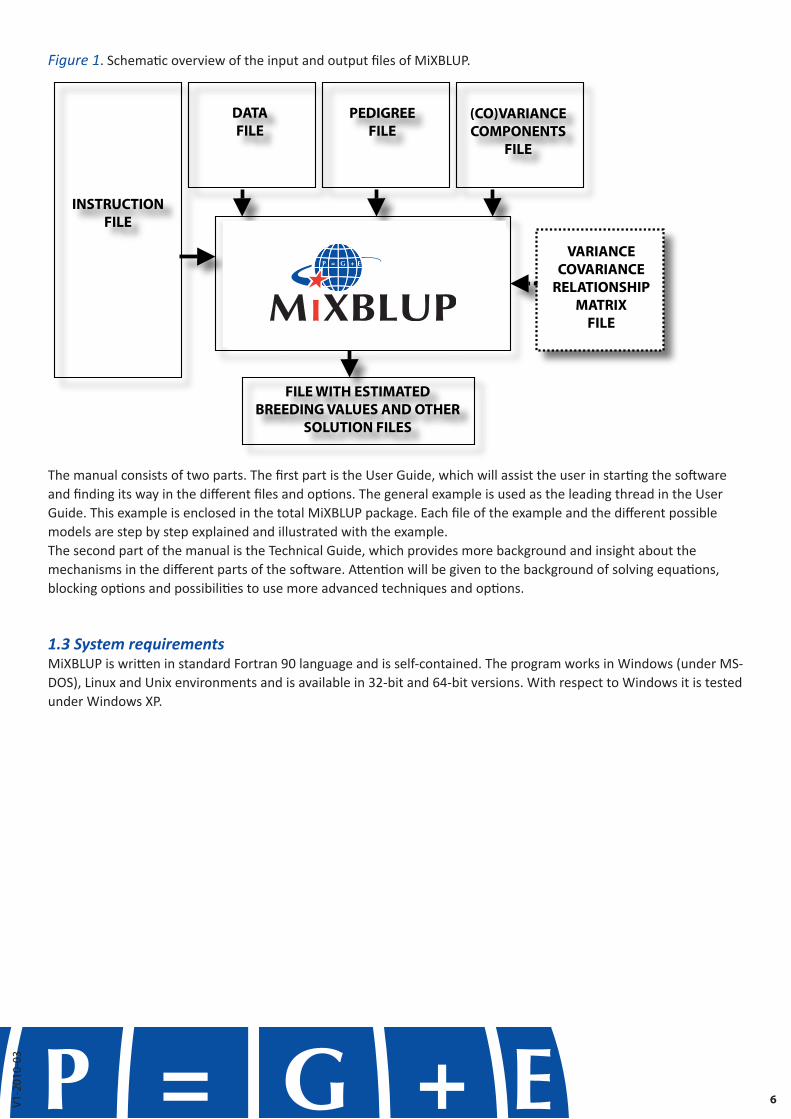
Figure 1. Schematic overview of the input and output files of MiXBLUP.

The manual consists of two parts. The first part is the User Guide, which will assist the user in starting the software and finding its way in the different files and options. The general example is used as the leading thread in the User Guide. This example is enclosed in the total MiXBLUP package. Each file of the example and the different possible models are step by step explained and illustrated with the example. The second part of the manual is the Technical Guide, which provides more background and insight about the mechanisms in the different parts of the software. Attention will be given to the background of solving equations, blocking options and possibilities to use more advanced techniques and options.

1.3 System requirementsMiXBLUP is written in standard Fortran 90 language and is self-contained. The program works in Windows (under MS-DOS), Linux and Unix environments and is available in 32-bit and 64-bit versions. With respect to Windows it is tested under Windows XP.

INSTRUCTIONFILE

DATAFILE

PEDIGREEFILE

(CO)VARIANCECOMPONENTS

FILE

VARIANCECOVARIANCE

RELATIONSHIPMATRIX

FILE

FILE WITH ESTIMATEDBREEDING VALUES AND OTHER

SOLUTION FILES

V1-

2010

-03

7

2 HOW TO START

2.1 Installing MiXBLUP softwareDownload the appropriate zip-file from http://www.mixblup.eu and unzip the folder with the executables: ‘reliabi-lities.exe’, ‘dataprocessor.exe’, ‘solver.exe’ and ‘MiXBLUP.exe’ in the work directory of your choice for Windows. For Linux the software needs to be installed in the bin directory.

2.2 MiXBLUP LicensesTo run MiXBLUP software on your computer you need a license. There are different license types for MiXBLUP. A license can be ordered at http://www.mixblup.eu. The trial license can handle complete datasets and will provide a maximum of 1000 solutions. This will give the user an opportunity to test the software and decide if it suits his needs. The small commercial license can be used for up to 1 million animal equations. This means that a single trait evaluati-on could be performed with up to 1 million animals in the pedigree. With multi-trait evaluations (n traits) the number of animals in the pedigree can be 1 million/n. The large commercial license, has no limit on the number of animal equations. The license key of the commercial licenses is computer specific. Therefore, if executables and the license key ‘LICENSE.DAT’ are moved to a new computer, an error message will be given by MiXBLUP. When a new computer is taken in use for an existing license a new license key should be requested at info@mixblup.eu with the LICREQST.DAT attached (how to generate a LICREQST.DAT file see below).

The characteristics of the different license types of MiXBLUP

License types License Time limit Limitations Trial License Not computer specific 1 month 1000 solutions Small commercial License Computer specific 1 year 1 million animal equations Large commercial License Computer specific 1 year Unlimited

2.3 License keyThe license key provides the information about the type and expiry date of the license. The trial license can be used for one month and the trial license key is not computer specific. The small and large commercial license can be used for one calendar year. The license key for these licenses is computer specific.

Trial LicenseOrder a trial license at http://www.mixblup.eu. After receiving your order, we send the necessary license key to the e-mail address stated in the order.

Commercial licensesOrder a commercial license at http://www.mixblup.eu. While entering the order you are asked to upload one ore more ‘LICREQST.DAT’ files. For each computer you need to upload a separate ‘LICREQST.DAT’ file. With this file we can generate a computer specific license key and send it to you.

V1-

2010

-03

8

Generating a ‘LICREQST.DAT’ file› Store the license key ‘LICENSE.DAT’ in the C:\MIXBLUP\bin-folder for Windows and in the /usr/bin-folder for Linux.› Run MiXBLUP.exe and enter the instruction file mixblup.inp. MiXBLUP.exe creates the file LICREQST.DAT in the working directory.› After payment of the license one or more ‘LICENSE.DAT’ files will be sent back and should be saved in the bin folder of the corresponding computer(s).

2.4 Example filesIn the MiXBLUP package, seven example files are enclosed. These files can be used to test if the software is running correctly and to get a feel for the program and the set-up of the files. The files should be saved in the work directory. The example files will serve as the leading thread in the upcoming paragraphs. Each file will be explained in further chapters with respect to its contents, syntax and criteria. Below a short description is given.

mixblup.inp instruction file for breeding value estimationdatafile.txt data file with phenotypes and effectspedfile.txt pedigree filepara.dat (co)variance components for the used random effectsibd.dat inverse identity-by-descent-matrix

V1-

2010

-03

9

3 INPUT FILES

The following files need to be made before starting MiXBLUP› a data file with the data to be analyzed› a pedigree file with relationship information› a (co)variance components file with variance and covariance components for the random effects, › an instruction file with information about the names of data file, pedigree file, covariance components file

and about the statistical models and some options for stopping criteria.› an optional file with an variance-covariance relationship matrix, such as an inverse identity-by-descent-matrix

(i.e. for marker-assisted breeding value estimation)

The input files are illustrated with an example with two body weight traits measured at two different ages. Different models are used for breeding value estimation to show the possibilities of MiXBLUP.

3.1 Data fileThe variables (animals/ effects/ traits) have each their own column in the data file. The data file is either free format, space separated or with fixed format. Data can be integer, alphanumeric and real values.

Example Columns in data file: animal ID, mean, herd, sex, dam ID, haplotype1, haplotype2, common environment, mate1, mate2, age1, age2, gene content, body weight at age1, bodyweight at age2

A11 1 1 1 A6 1 2 1 A12 A13 100 200 1 1200 2000 A12 1 1 2 A6 2 1 1 A11 A13 101 203 1 1280 2100 A13 1 1 1 A7 1 2 2 A11 A12 99 199 1 1100 1900 A14 1 1 2 A7 2 2 2 A15 A16 102 198 2 1250 1800 A15 1 2 1 A8 2 1 3 A14 A16 90 201 1 1150 2200 A16 1 2 2 A8 2 1 3 A14 A15 95 203 1 1000 2050 A17 1 2 1 A9 1 2 4 A18 A19 103 205 1 1300 1950 A18 1 2 2 A9 2 2 4 A17 A19 105 195 2 1250 2080 A19 1 2 1 A10 1 1 5 A17 A18 110 199 0 1280 1920

3.2 Pedigree file The pedigree file consists of the animal Identification number (ID) and their sire and dam IDs in the first three columns. The columns must be separated by at least one space. Additionally the pedigree file may contain other information in additional columns. Each animal with a record in the data file, or which is coded as maternal, paternal or mate effect (i.e. group selection) must be in the pedigree file. Animals that do not appear in the data file, but that appear as sire or dam in the pedigree file must have also their own record in the pedigree file. In other words, the pedigree in the pedigree file must go back to the phantom parents groups. Animal IDs are assumed to be of same type as the animal ID in the data file (either numeric or alphanumeric). The phantom parent groups need to be coded as negative integers. When a sire model or animal model without phantom parent groups is used (specified in the instruction file), then missing sires and dams (or maternal grand sires) can be coded with a zero (0) or a negative integer number. When marker-assisted BLUP is performed and one is interested in the QTL-haplotype effects per animal and a total EBV, then the pedigree file needs to contain the haplotypes for each animal. With multiple QTL in the model the haplotypes should be given in the order as given in the model.

Example Columns in pedigree file: animal ID, sire ID, dam ID

A1 0 0 A2 0 0 A3 0 0 A4 0 0 A5 0 0 A6 0 0 A7 0 0 A8 0 0 A9 0 0 A10 0 0 A11 A1 A6 A12 A2 A6 A13 A3 A7 A14 A4 A7 A15 A5 A8 A16 A1 A8 A17 A2 A9 A18 A3 A9 A19 A4 A10

3.3 (Co)variance components fileThe (co)variance components file contains the variance-covariance matrices of random effects in the model. There are two options for the format of the file: (1) in lower triangular matrix form and (2) in sparse matrix form.

3.3.1 Lower triangular matrixIn the lower triangular matrix, the (co)variance components file can be specified in lower triangular matrix form using trait names to identify the components. This is the most user-friendly way and is recommended. The name of the random effect is given on top of the matrix and the names of the traits are given in front of the matrix.

› The (co)variances for the traits specified in the lower triangular matrices can be given in any order, i.e. the order given in the model section of the directive file is not leading.

› Models should include at least an animal effect and a residual effect.› The number of traits in the matrices can be larger than the number of traits specified in the model section.

Only the lines for which the name has been specified in the model section will be used in MiXBLUP. › The order of the column names is assumed to be the same as the order of row names.› Restriction: if marker-assisted breeding value estimation is performed with the use of IBD matrices, then

each variance-covariance matrix needs to be named and numbered, e.g. GIV1, GIV2, etc. The name GIV refers to the use of the General Inverse Variance (GIV) function in the model. The order is assumed to be identical to the order as given in the model lines in the instruction file.

› In the case of multiple genetic effects (e.g. animal, dam, mate), it should be specified within brackets whether it is the genetic variance of animal, dam or mate.

› If the model contains random regression(s) on animal all regression term(s) should be specified (e.g. animal*covar1 and animal*covar2). See example D random regression /testday model.

› In case of group selection with multiple mate effects in the model, the first group mate effect in the model should be specified (e.g. mate2*mate2_x). See example J group selection.

V1-

2010

-03

10

V1-

2010

-03

11

Example The lower triangular (co)variance components file with two traits (bodyweight1 and bodyweight2) with random animal genetic effects and residual effects. G bw1(animal) 3000 bw2(animal) 2939 4500 residual bw1 7000 bw2 1715 10500

3.3.2 Sparse matrix formatIn the sparse matrix form, the (co)variance components file must have the same order of the matrices specified as the order of random effects listed in the model. The random animal effect should be the last random effect in the model and its (co)variances should appear in the sparse matrix file just before the residual (co)variances. The residual (co)variance matrix should be specified at the end of the sparse matrix file. The values are given with the random effect number, row number, column number and the value of the (co)variance); row and column number can be switched.. Off-diagonals can be skipped if they are zero. First, all the non random genetic effects should be listed in the order as described in the manual, subsequent the (co)variances related to the animal genetic effects and finally the (co)variances of the residual effects.

Example The Sparse matrix file with two traits with a random animal genetic effect and a residual effect Columns: random effect, row number, column number and value of the (co)variance.

1 1 1 3000 #animal 1 2 1 2939 1 2 2 4500 2 1 1 7000 #residual 2 2 1 1715 2 2 2 10500

When haplotypes are used in the model for marker-assisted breeding value estimation with the use of an IBD-matrix, both are counted as effects, but the second haplotype does not need to have variance components, when it is combined to the first haplotype. See example I Marker-assisted BLUP with an IBD-matrix.

3.4 Variance-covariance relationship matrixIn some cases random effects have a different variance-covariance structure (CV-matrix) than simply a diagonal matrix or the A-matrix as for additive genetic effects. Examples of other relationship matrices are IBD-matrices for marker-assisted breeding value estimation for a limited number of QTL or dominance relationship matrices. These matrices cannot be made by MiXBLUP, but can be read by MiXBLUP separately.The file with the elements of the variance-covariance relationship matrix should contain all non-zero elements constructed as: row_number, column_number, inverse matrix value. The order and numbers used as row and column numbers should correspond to the ID (e.g. haplotype numbers with marker-assisted breeding value estimation) used in the data file. Box 5 gives the inverse IBD matrix for the general example with only two haplotypes.

Points of interest when designing the matrix› The inverse IBD-matrix should contain at least one off-diagonal.› Zero off-diagonals can be omitted.› Since the matrix is symmetric, only the lower triangular matrix needs to be given (invIBD(2,1)=invIBD(1,2)).

V1-

2010

-03

12

Example The inverse variance-covariance relationship matrix, e.g. inverse IBD matrix(2 haplotypes that have relationship of 0.25 amongst each other).Columns: number of the row, number of the column, inverse matrix value.

1 1 1.06 1 2 -0.26 2 2 1.06

V1-

2010

-03

13

4 INSTRUCTION FILE

In the instruction file, the names and locations of the other input files are stated, the variables that can be found in the input files are stated and the models that should be used are defined. In the following paragraphs, the different sections of the instruction file will be discussed and the contents and options for each of those sections will be explained. Below the example instruction file is given for a bivariate animal model for body weight 1 and body weight2. Example The Instruction file for a bivariate animal model

TITLE breeding value estimation for bodyweight 1 and bodyweight 2

DATAFILE datafile.txt animal A mean I herd I sex I dam A haplo1 I haplo2 I commonenv I mate1 A mate2 A age1 R age2 R genecontent R bw1 T bw2 T

PEDFILE !groups 0.0 animal A sire A dam A

PARFILE para.dat

CVMATRIX # optional, necessary when using variance-covariance relationship matrices other Ibd.giv # than numerator relationship matrix Ibd2.giv

MODEL bw1 ~ herd sex !random G(animal) bw2 ~ herd sex !random G(animal)

SOLVING !maxit 1000

V1-

2010

-03

14

4.1 TitleThe instruction file starts with a specification of the title of the analysis. The TITLE section is optional, if omitted the first comment line (indicated by #) is used as the title of the analysis.

4.2 Data fileThe instruction file specifies the name of the data file, the variables that can be found in this file and the type of the variables. The data file is located by default in the work directory, but can be in another folder if specified in the name of the file (e.g. d:\datafile\datafile.txt). The order of the variables should be the same as the order of the columns in the data file.

Syntax: DATAFILE <filename> [field 1] [type: I/R/T/A] …… [type: I/R/T/A] [field n] [type: I/R/T/A]

Type: Defines the type of the variable in this field. Available types are I, R, T and A. I for integer values R for real values T for trait A for alphanumerical values

Options: !missing <value> Value is the value considered for missing value !block This column is used as block variable, the data file and pedigree file need to contain

this column and both need to be sorted on this column. It is necessary for calculation of reliabilities, but might be beneficial in some computationally heavy genetic evaluations.

The variable must be integer. !skip [value] With this one (!skip 1) or multiple (e.g. !skip 2) header line(s) in a data file can be omitted

Comments:› Maximum length of field names is 8 characters.› When data is alphanumeric, the symbols ‘:’ and ‘-’ can be used, but ‘/’ can not be used.› Alphanumeric codes should not contain spaces.› If !block is specified for multiple datafields, only the first specification is used. It affects the SORTED-line in

the file generated by the parser (dataprocessor.inp or dataprocessor_rel.dir).› Alphanumeric values (coded with A) are translated into numerical values.› Each alphanumerical value in the data file gets a unique numerical value, there is no apparent relation

between the alphanumerical and numerical values, e.g. the sequence/order will differ.› If the animal ID is alphanumeric (numeric), the first three columns in the pedigree are considered to be

alphanumeric (numeric) as well.

4.3 Pedigree fileThe instruction file specifies the pedigree file name The pedigree file is located by default in the work directory, but can be in another folder if specified in the name of the file (e.g. d:\pedfile\pedfile.txt). The default field format assumed is: (1) animal ID, (2) sire ID and (3) dam ID. Without using a blocking variable, the pedigree file does not need to be sorted. Optionally a block variable can be given as column 4. In that case the pedigree file should be sorted on the block variable as well as the data file. Sire models with sires and maternal grandsires in the pedigree file is not possible.

V1-

2010

-03

15

Options: !groups[value] This option means that random genetic phantom parent groups are included in the

pedigree. These need to have negative integers. If phantom parent groups are used, with [value] it is possible to specify whether these group effects should be modelled as fixed (value=0) or as random (value>0.0), the larger the value the more random it is, or the more estimates are regressed towards the mean.

Comments:› If the first field of the pedigree file corresponds exactly (case-sensitive comparison) with an alphanumerical

field (coded with A in the data file section), then all values in the pedigree file are handled as alphanumerical values. That is, they are translated into numerical values. The translated version of the pedigree file is ‘pedigree.txt’.

› If the first field corresponds with an alphanumerical field, then also the fields for sire and dam in the data section (if present) must be defined as alphanumeric.

› When marker-assisted BLUP is performed and one is interested in the QTL-haplotype effects per animal and a total EBV, then the pedigree file needs to contain the haplotypes for each animal. With multiple QTL in the model the haplotypes should be given in the order as given in the model.

4.4 (Co)Variance components fileThe instruction file specifies the name of the (co)variance components file. The (co)variance components file is located by default in the work directory, but can be in another folder if specified in the name of the file. The (co)variance components file can be in two different formats. The default format is in lower triangular matrix form. The other format is the sparse matrix form. The lower triangular form gives great flexibility. If the sparse format is used, the option !sparse needs to be used.

Syntax: Default format: lower triangular matrix form PARFILE <filename>

Other format: sparse format PARFILE <filename> !sparse

4.5 Variance-covariance relationship matrixThe name of the inverse variance-covariance matrices, e.g. inverse IBD-matrices can be given below the CVmatrix (covariance matrix). The file with the variance-covariance relationship matrix file is located by default in the work directory, but can be in another folder if specified in the name of the file. The order is important and should correspond with the numbers given in the General Inverse Variance function (GIV function). The inverse IBD-matrix should contain all non-zero elements constructed as: row_number, column_number, invIBD-value. The file should not contain alphanumeric data. The inverse IBD-matrix should contain at least one off-diagonal.

V1-

2010

-03

16

4.6 ModelThe MODEL line specifies the start of the model lines. Below the MODEL line, for all traits the models are given on a separate line. For each trait, we start with the name of trait followed by ‘~’; subsequently the fixed effects and finally, after the !random qualifier, the random effects are specified. Models need to have always at least one fixed effect and one random animal genetic effect, besides a residual. Random animal genetic effects need to be given with the function G( ), (e.g. G(animal), so that MiXBLUP uses pedigree relations to construct the numerator relationship matrix or additive genetic relationship matrix. Hereafter we discuss a number of more complex models.

4.6.1 Fixed regressionsWe should first distinguish between general and nested regressions. For general regression the covariable can just be listed as factor in the model. Because it is listed as a real number and not an integer, the software knows that the effect is a covariable.

Example Section of the instruction file that codes for the model with general fixed regression.

MODEL bw1 ~ sex age1 !random G(animal) bw2 ~ sex age2 !random G(animal)

Example Section of the instruction file that codes for the model with a fixed regression covariable nested within a fixed effect.

MODEL bw1 ~ herd sex age1*sex !random G(animal) bw2 ~ herd sex age2*sex !random G(animal)

4.6.2 Fixed effects within blockPutting fixed effects within block may have sometimes computational advantages in breeding value estimation, especially when the fixed effect has many levels. For calculation of reliabilities and accounting for inaccuracy of the fixed effects, e.g. a fixed effect with many levels such as HYS, it is necessary to put the fixed effect to be accounted for within block. Fixed effects can be put within block by using the BL-function.

Example Section of the instruction file that codes for the model with a fixed effect within block.

MODEL bw1 ~ BL(herd) sex !random G(animal) bw2 ~ BL(herd) sex !random G(animal)

4.6.3 Random regressionsFor random regression a distinction needs to be made between general random regression and random regression for animal genetic effects (e.g. test-day models). When a general regression should be considered as random, a dummy integer column (mean, column with ones) should be used as dummy. For random regression ”int*real” is treated as equal to “real*int”, the order in which these variables are specified is free.

Example Section of the instruction file that codes for the model with general random regression on age and the (co)variance components file.

MODEL bw1 ~ herd sex !random mean*age1 G(animal) bw2 ~ herd sex !random mean*age2 G(animal)

(Co) variance components file mean bw1 1.0 bw2 0.5 1.0

G bw1(animal) 3000 bw2(animal) 2939 4500 residual bw1 7000 bw2 1715 10500

This model can also be used for random regression on marker gene contents or number of haplotype copies as described in Mulder et al. (2010a,b).

Example Section of the instruction file that codes for the model random regression on marker gene contents of number of haplotype copies.

MODEL bw1 ~ herd sex !random mean*genecontent G(animal) bw2 ~ herd sex !random mean*genecontent G(animal)

Example Section of instruction file that codes for the model with genetic random regression on age and the variance-covariance file.

MODEL bw1 ~ herd sex !random G(animal,animal*age1) bw2 ~ herd sex !random G(animal,animal*age2)

(Co) variance components file G bw1(animal) 3000 bw2(animal) 2939 4500 bw1(animal*age1) 0.0 0.0 100 bw2(animal*age2) 0.0 0.0 0.0 200

residual bw1 7000 bw2 1715 10500

V1-

2010

-03

17

V1-

2010

-03

18

4.6.4 Social interactionsGroup selection is implemented in MiXBLUP. It can be either used for groups with constant group size or for variable group size. When groups are of equal size than one can define the genetic associative effects or social breeding values as G(animal, mate2 and mate3 and mate4 etc). In the (co)variance components file in sparse-format the variance of the social effects gets the same number as the genetic effects, similar to maternal genetic effects. With a (co)variance components file in lower triangle it works the same as with maternal genetic effects (see 3.5.7.6). When groups do not have equal group size, one needs to define the evaluation as for the group with the maximum size. The groups with less animals need to have a dummy animal as mate. This dummy animal needs to be added to the pedigree file as well with sire and dam as 0 and 0 (unknown). In addition one should use random regression on an indicator variable which is 0 or 1. So in the case of the dummy animal, the indicator is 0, in other cases it is 1. In this way, the dummy animal will have no effect on the breeding value estimation. These indicator columns 0/1 need to be provided by the user, as well as the complete data file and pedigree file. To combine the effects of different mates to one design matrix, one can use the ‘and’ function. There are a few constraints that can not be done with combining of effects; all of them will hardly appear:When ‘and’ is used for group selection, it can not be used anymore for IBD-haplotypes or in other words one can not include haplotype effects and group selection in one model.Combining of effects needs to be the same for all traits, in other words it assumes that the animal is in one group his whole life and not in different groups with different sizes. But the parser can handle that some traits have social genetic effects whereas others have not.There can be only one group of combined genetic effects, so there should be no commas placed between the effects. Basically it means that the genetic effects can be only combined to one other effect and not to more.The order of genetic effects should be kept the same across models with group selection. This means that for all traits the order should be either G(animal,mate2 and mate3) or G(mate2 and mate3, animal), but not for some traits G(animal,mate2 and mate3) and for others G(mate2 and mate3, animal).

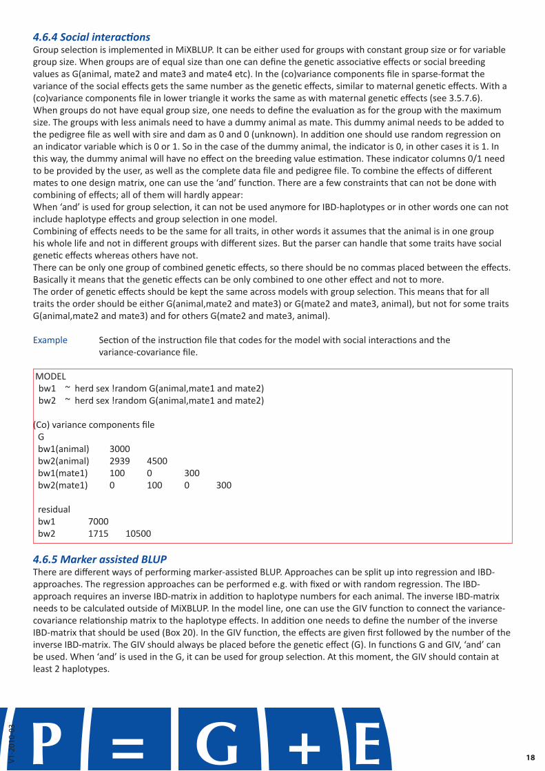
Example Section of the instruction file that codes for the model with social interactions and the variance-covariance file.

MODELbw1 ~ herd sex !random G(animal,mate1 and mate2)bw2 ~ herd sex !random G(animal,mate1 and mate2)

(Co) variance components fileG bw1(animal) 3000 bw2(animal) 2939 4500 bw1(mate1) 100 0 300 bw2(mate1) 0 100 0 300

residual bw1 7000 bw2 1715 10500

4.6.5 Marker assisted BLUPThere are different ways of performing marker-assisted BLUP. Approaches can be split up into regression and IBD-approaches. The regression approaches can be performed e.g. with fixed or with random regression. The IBD-approach requires an inverse IBD-matrix in addition to haplotype numbers for each animal. The inverse IBD-matrix needs to be calculated outside of MiXBLUP. In the model line, one can use the GIV function to connect the variance-covariance relationship matrix to the haplotype effects. In addition one needs to define the number of the inverse IBD-matrix that should be used (Box 20). In the GIV function, the effects are given first followed by the number of the inverse IBD-matrix. The GIV should always be placed before the genetic effect (G). In functions G and GIV, ‘and’ can be used. When ‘and’ is used in the G, it can be used for group selection. At this moment, the GIV should contain at least 2 haplotypes.

V1-

2010

-03

19

When one wants to perform marker-assisted BLUP according to Fernando and Grossman (1989), the haplotypes and inverse IBD-matrix should be made in advance of running MiXBLUP. The haplotypes should be added to the data file and to the data file. When the haplotypes are added to the pedigree file MiXBLUP will generate the haplotype EBV per animal and the total EBV.

Example Instruction file with marker-assisted BLUP and the (co)variance components file with marker-assisted BLUP.

TITLE Breeding value estimation for bodyweight 1 and bodyweight 2

DATAFILE datafile.txt animal A mean I herd I sex I dam A haplo1 I haplo2 I commonenv I mate1 A mate2 A age1 R age2 R genecontent R bw1 T bw2 T

PEDFILE pedfile.txt !groups 0.0 ! animal A sire A dam A haplo1 I #comment: if provided then EBVhap and EBVtot are calculated haplo2 I

PARFILE para.dat

CVmatrix ibd.dat

MODEL bw1 ~ herd sex !random GIV(haplo1 and haplo2,1) G(animal) bw2 ~ herd sex !random GIV(haplo1 and haplo2,1) G(animal)

SOLVING !maxit 1000 !stopcrit 1.0e-10

V1-

2010

-03

20

(Co)variance components file

GIV1 bw1 200 bw2 100 200

G bw1(animal) 3000 bw2(animal) 2939 4500 residual bw1 8000 bw2 1715 10500

4.6.6 Maternal genetic effectsFor some traits direct and maternal genetic effects exist, so one would like to model both.

Example Section of the instruction file that codes for the model with maternal genetic effects and the (co)variance components file with maternal genetic effects. MODEL bw1 ~ herd sex !random G(animal,dam) bw2 ~ herd sex !random G(animal,dam)

(Co)variance components file G bw1(animal) 3000 bw2(animal) 2939 4500 bw1(dam) 100 0 300 bw2(dam) 0 100 0 300 residual bw1 7000 bw2 1715 10500

V1-

2010

-03

21

4.6.7 Maternal genetic and common environmental effectsThe model is the same as the model with a maternal genetic effect, but the model is now extended with a common environmental effect (e.g. litter effect).

Example Section of the instruction file that codes for the model with maternal genetic and common environmental effects and the (co)variance components file with maternal genetic and common environmental effects.

MODEL bw1 ~ herd sex !random commonenv G(animal,dam) bw2 ~ herd sex !random commonenv G(animal,dam)

(Co)variance components file commonenv bw1 1.0 bw2 0.5 1.0

G bw1(animal) 3000 bw2(animal) 2939 4500 bw1(dam) 100 0 300 bw2(dam) 0 100 0 300

residual bw1 7000 bw2 1715 10500

V1-

2010

-03

22

4.7 Solving and Output Options

ReliabilitiesMiXBLUP offers the possibility to calculate approximate reliability of the EBVs of animals, except for models with inverse IBD-matrices. To calculate reliabilities, the option !reliability should be put in the SOLVING section in the instruction file and a model with only one fixed effect per trait should be used. For reliabilities only one fixed effect can be used in the model, so the model lines should be changed and a different instruction file than used for prediction of EBV should be used. Usually the fixed effect with the most classes and so with the least accuracy of estimation is kept in the model. The fixed effects needs to be within block (BL(fixed effect)). For models with maternal genetic effects reliabilities.exe is called twice automatically: for direct EBVs and for maternal genetic EBVs.

The data file and pedigree file need to contain the block variable (!block) and both need to be sorted on this column. As a consequence of these changes, the instruction file (mixblup_rel.inp) and pedigree file (pedigree_block.txt) are slightly different in this case.

Example Instruction file with calculation of reliabilities.

TITLE Reliabilities for bodyweight 1 and bodyweight 2

DATAFILE datafile.txt animal A mean I herd I !block sex I dam A haplo1 I haplo2 I commonenv I mate1 A mate2 A age1 R age2 R genecontent R bw1 T bw2 T

PEDFILE pedigree_block.txt!groups 0.0 animal A sire A dam A herd I #comment: block code, add extra column

PARFILE para.dat

MODEL

# blocking of herd, in calculation of reliabilities is herd approximated bw1 ~ BL(herd) !random G(animal) bw2 ~ BL(herd) !random G(animal)

SOLVING !reliability

V1-

2010

-03

23

There are a number of options for solving the equations. They can be grouped in the Solving section. The section can be omitted when default values for maximum number of iterations (5000) and stopping criteria (1.0e-4) are applicable, but can be used to run the programs with user specified values.

Options: !maxit <n2> Number of maximum iterations performed in the analyses. Values entered in this section

are passed on to the file stopping_criteria.dir. !stopcrit The user specified maximum relative difference in solutions from one iteration to the next

iteration. !restart If this qualifier is used, a restart will be done on old solutions. If restart is used together

with alphanumeric data then the same alphanumerical coding will be applied (if possible). !baseanimalszero The solution in the Solani.txt file is adapted to make the average value over the base

animals equal to zero. The animal ID of the base animals should be given in the file BaseAnimals.dat (one number per row). Phantom parent groups can also be included in the base by including negative numbers in BaseAnimals.dat. The averages per trait that are used as adjustment terms are included in the log file MiXBLUP.log. If not all animals or phantom groups are present in the data file, then a message is given in the log file

MiXBLUP.log. If the animal ID is alphanumeric then alphanumerical values should be given in the file BaseAnimals.dat.

!reliability Reliabilities are calculated instead of EBV.

V1-

2010

-03

24

5 RUNNING MiXBLUP

5.1 Run without old solutionsSolving mixed model equations using MiXBLUP involves execution of four programs. The main executable is MiXBLUP.exe. This is the parser and calls dataprocessor.exe, solver.exe and reliabilities.exe.

The executables need to be run either under Linux or in a Command prompt (MS-Dos) under windows. There are two ways: 1. by entering information on the command line or 2. in batch mode.

If MiXBLUP.exe is run on the command line, MiXBLUP.exe is asking for the name of instruction file that should be typed on the screen. If MiXBLUP.exe is run in a batch mode, it can be done as follows. Firstly, make a file that contains only the name of the instruction file. Secondly, make a batch file as follows (mixblup.bat) that contains the following: MiXBLUP.exe<nameinstructionfile.txt>execution.log Do not call the outputfile MiXBLUP.log, because that file is made already by MiXBLUP.exe

5.2 Run with restart on old solutionsIf there is more data accumulated and a restart is wanted, the only additional file necessary for a restart is the Solunf file. If !restart is used, MiXBLUP renames Solunf to Solold. If Solold is present, the pre-processor dataprocessor will create a file with a solution vector called ‘Solvec’. This file will be used to preset the solution vector of the MME before the start of the iteration process (in solver). Aside from the Solunf file, the data file, pedigree file, (co)variance components file and the instruction file need to be known to MiXBLUP, as usual.

5.3 Monitoring processAfter the run is finished, it is worth to look through the different log-files. In MiXBLUP.log some information is given about preprocessing/postprocessing the data. It also lists error messages. If a mistake is made somewhere or the variance-covariance matrix, variance-covariance matrix, is not positive definite, it is likely that at least the solver.exe does not run. Check in that case the dataprocessor.log, because it may give some indications for errors. If all programs have run successfully, it is worth to check the solver.log, to see how the convergence was reached. In cases with poor convergence, it will give a warning and some model checking may be appropriate. When reliabilities are calculated, one can check the reliabilities.log or reliabilities_direct.log/reliabilities_indirect.log when reliabilities are calculated for direct and indirect genetic effects, such as maternal genetic effects.

V1-

2010

-03

25

6 OUTPUT FILES

6.1 Solution filesThe solution files are split up into standard output files and postprocessed solution files. Postprocessed solution files are generated only in specific cases, such as alphanumeric data, use of a reference population (!baseanimalszero) or marker-assisted breeding value estimation with IBD-matrices.

6.1.1 StandardThe standard output is Solfix.txt for solutions of fixed effects across blocks (default), Solani.txt for EBV, Relani.txt for reliabilities, Solr0#.txt for each random effect other than genetic effects, Solf0#.txt for fixed effects within blocks (use of BL( )) and Solreg.txt for general regressions. Here we give the description of the output-files for different models of the general example (see 4.6).

Table 1 shows the format of the Solani.txt file. If maternal genetic effects or mate effects (group selection) are present, (see 4.6.6) the maternal EBV can be found at the end.

Table 1: Solani.txt”-File: Solutions for direct genetic animal effects and indirect (e.g. maternal genetic effects or mate effects/social EBV)

Column Description 1 Animal ID 2 Number of descendants 3 Number of Observations 4 Direct EBV for trait 1 5 Direct EBV for trait 2 6 Indirect EBV for trait 1 7 Indirect EBV for trait 2

Table 2 shows the format of the Relani.txt file. In the case of maternal genetic effects, two Relani.txt files are generated: 1. “Relani_direct.txt”: file with direct reliabilities and 2. “Relani_indirect.txt”: file with maternal genetic reliabilities.

Table 2: Relani.txt”-File: Solutions for Animal Effects

Column Description 1 Animal ID 2 Number of descendants 3 Number of Observations 4 Direct EBV for trait bw1 5 Direct EBV for trait bw2

Table 3 shows the Solfix.txt file with solutions for across-block fixed effects.

Table 3: Solfix.txt”-File: Solutions for Across-Block Fixed Effects Column Description 1 Factor Number 2 Trait Number 3 Level Code 4 Number of Observations 5 Direct EBV for trait 2 6 Solutions 7 Name of Trait

V1-

2010

-03

26

In case fixed effects are within block (BL(fixed effect)) than solutions are in the Solf#.txt file, where # indicates the number of the within-block effect. Table 4 shows the Solf01.txt file for example with the model with a fixed regression covariable nested within a fixed effect (4.6.2).

Table 4: Solf01.txt”-File: Solutions for Within-Block Fixed Effect

Column Description 1 Level Code 2 Number of Observations 3 Solutions for trait 1 (bw1) and Factor herd 4 Solutions for trait 2 (bw2) and Factor herd

When the model includes general fixed regressions then a Solreg.txt file is created with the solution of the general regression (table 5).

Table 5: “Solreg.txt”-File: Solutions for General Regressions

Column Description 1 Trait Number 2 Regression Number within Trait 3 Solution 4 Name of Trait 5 Name of Covariable

In case we have non-genetic random effects, e.g. common environmental effects than Solr0#.txt are generated with solutions for the levels of that random effect. Table 6 shows the solution file Solr01.txt for the random effect commonenv . See example: Section of the instruction file that codes for the model with maternal genetic and common environmental effects in 4.6.7

Table 6: Solr01.txt”-File: Solutions for Random Effect 1 (commonenv)

Column Description 1 Level Code 2 Number of Observations 3 Solution for Trait 1 (bw1) and Factor commonenv 4 Solution for Trait 2 (bw2) and Factor commonenv

“Solunf”:Contains all solutions to the MME. Solutions in this file can be used as initial values for later estimation when more date has been accumulated. if !restart is used the Solunf is renamed to Solold. If Solold is present, the pre-processor dataprocessor will create a file with a solution vector called ‘Solvec’. This file will be used to preset the solution vector of the MME before the start of the iteration process (in solver).

6.1.2 Post processed output filesIf alphanumeric data exists in the data file, it needs to be recoded to numeric values to run dataprocessor.exe and solver.exe. After finishing solver.exe, the solutions are recoded back to their original alphanumeric codes by MiXBLUPB.exe. The Solani.out contains the recoded file with EBV. When the option !baseanimalszero is used, Solani.out contains the EBV after adjusting them to the base of the reference population. The lay-out of Solani.out is the same as for Solani.txt.If fixed effects contain alphanumeric data, the Solfix.out is created giving the solutions of the fixed effects recoded back to alphanumeric codes. The format is the same as that of Solfix.txt.

If other random effects are alphanumeric, the Solr#.out contains the solutions for the levels of the random effect recoded back to alphanumeric codes. The format is the same as that of Solr#.txt.

V1-

2010

-03

27

When marker-assisted breeding value estimation with IBD-matrices is performed, MiXBLUP creates EBVhap# with the estimated haplotype effects for each animal for QTL#. The format in EBVhap is given in Table 7.

Table 7: EBVhap1”-File:Estimated haplotype effects

Column Description 1 Animal 2 Estimate for haplotype 1 for trait 1 3 Estimate for haplotype 2 for trait 1 4 Estimate for haplotype 1 for trait 2 5 Estimate for haplotype 2 for trait 2

The total EBV is given in EBVtot and is calculated per animal as the sum of the polygenic effect and the haplotype effects. The polygenic EBV and QTL-EBV are equally weighted. The format is simply the animal ID followed by the total EBV for all traits. The order of the traits is the same as in the Solani.txt file.

6.2 Log filesMiXBLUP.log Log-file of MiXBLUP OK_dataprocessor Dataprocessor ran successfullyOK_solver Solver ran successfullyOK_reliabilities Reliabilities ran successfullyWarning.log Gives warning MiXBLUP.lst Contains a short summary of dataprocessor and summary statistics of the dataDataprocessor.log Extensive log-file of dataprocessor, gives also errorsSolver.log Log-file of solver. It gives the convergence and a description of output filesReliabilities.log Log file of reliabilities for direct genetic effectsReliabilities_indirect.log Log file of reliabilities for maternal genetic effectsMemory.txt Contains information about the amount of random access memory used during the

execution of the programs. In practice, the amount actually is often larger due to memory overhead and depends on the computer.

Modlog.txt Contains model and data parameters.

In some cases, the log files can not be read by Notepad. In that case, use of other text editor software programs, such as ConTEXT or Programmer’s File Editor (both freely available), are recommended.

6.3 Temporary filesInstruction.inp Temporary file used – contains an updated version of the input file for the parserData99.tmp Tempory data file used when converting alphanumeric dataData.txt Transformed data file used by dataprocessorPedigree.txt Transformed pedigree file used by dataprocessorCovar.txt Parameter file with variance-covariance matrices in dataprocessor formatDataprocessor.inp Directive file for dataprocessorStopping_criteria.inp File with stopping criteria for solverSolani.tmp Intermediate version of Solani.txt file (only in case of alphanumerical coding or when

the baseanimalszero option is used)Code.inp In case of alphanumerical coding, the line number of the string is the code that

corresponds to the value.

V1-

2010

-03

28

7 TUNING MiXBLUP

7.1 Flow of programsThe software consists of four executables all with their own role (Figure 2). The main executable is MiXBLUP.exe. MiXBLUP.exe calls dataprocessor.exe and Solver.exe and if required reliabilities.exe according to user instructions. Basically dataprocessor.exe does some preprocessing of the data and does many data checks. Solver.exe writes the breeding values to the Solani.txt file in addition to other solution files. The program reliabilities.exe calculates approximate reliabilities for the estimated breeding values (EBV) and writes the reliabilities to the Relani.txt file.

Figure 2. Schematic overview of input, output and the role of the executables of the MIXBLUP-software package.

7.2 Variance covariance matrices not positive definiteThe dataprocessor.exe checks whether the used variance-covariance matrices given in the variance-covariance file are positive definite. If the matrix is not positive definite, the dataprocessor.exe will stop immediately and gives in dataprocessor.log an indication which variance –covariance matrix is not positive definite. The user should bend this matrix, e.g. with existing methods as presented in literature (Hayes and Hill, 1981; Jorjani et al., 2003). The best practice is to check beforehand the eigenvalues of all matrices.

!

!

INSTRUCTIONS FILE DATA FILE PEDIGREE FILE(CO)VARIANCE

COMPONENTS FILE

MiXBLUP.exe

Parser program: some pre- andpostprocessing and call of other

dataprocessoer.exe

Preprocessing + checks data and

Solver.exe

Solves mixed modelequations EBV

Reliabilities.exe

Calculates approximatereliabilities of breeding

Estimated breeding values Reliabilities

V1-

2010

-03

29

7.3 Convergence problemsIn all cases it is wise to check the solver.log to see the convergence characteristics. It will give an indication whether the convergence was poor or slow. In some cases MiXBLUP does not converge easily or does not converge at all. In those cases, a number of things should be checked:

› Check whether fixed effects are confounded amongst each other › Check whether fixed effects and phantom parent groups are confounded › Does the run include traits that are highly correlated (genetic correlation > 0.9)?› A mismatch between used variance-covariances and the current values, e.g. when using an old set of

variances and covariances.

A useful comparison is to compare estimates of EBV and fixed effects of different programs, e.g. MiXBLUP and ASREML/DMU.

A few solutions to problems› Simplification of the model, e.g. remove some confounded fixed effects.› Add a value to diagonal of phantom parent groups to regress poorly estimable phantom parents groups back

to mean (!groups value). This value could be like 1.0, 3.0 or 5.0. The higher the value the more the estimate is regressed towards the mean (Schaeffer, 1994).› Re-estimate all variances and covariances.› If traits are highly correlated, traits might be combined to one trait and observations might be used as

repeated observations (repeatability model).› Very high correlations (> 0.90) might be bended to values of 0.90.› Split up the evaluation into a few evaluations, e.g. of groups of traits that are more correlated amongst each

other because of biological similarity.

7.4 Optimisation of memory and time<>In very large genetic evaluations with millions of records and animals in the pedigree, it may help to put fixed effects with an extremely large number of equations, such as herd-year-season effects within block with the function BL(fixed effect).

In some cases memory might be limited especially when working with 32-bit versions of the software. When 64-bit computers are available, 64-bit versions of the software should be used so that a larger amount of memory can be utilized.In some case it might be wise to split up very large genetic evaluations into a few smaller evaluations.

V1-

2010

-03

30

8 REFERENCES

Fernando, RL, and M. Grossman, 1989. Marker assisted selection using best linear unbiased prediction. Genet. Sel. Evol., 21: 467-477.

Hayes, J.F., and W.G. Hill, 1981. Modification of estimates of parameters in the construction of genetic selection indices (“Bending”). Biometrics 37: 483-493. Jorjani, H., L. Klei, and U. Emanuelson. 2003. A simple method for weighted bending of genetic (co)variance matrices. J. Dairy Sci. 86:677-679.

Jorjani, H., L. Klei, and U. Emanuelson. 2003. A simple method for weighted bending of genetic (co)variance matrices. J. Dairy Sci. 86:677-679.

Mulder, H. A., M. P. L. Calus, and R. F. Veerkamp. 2010a. Prediction of haplotypes with missing genotypes and its effect on accuracy of marker-assisted breeding value estimation. Genet. Sel. Evol. accepted.

Mulder, H. A., T. H. E. Meuwissen, M. P. L. Calus, and R. F. Veerkamp. 2010b. The effect of missing marker genotypes on the accuracy of gene-assisted breeding value estimation: a comparison of methods. Animal 4:9-19.

Schaeffer, L.R. and J.C.M. Dekkers, 1994. Random regressions in animal models for test-day production in dairy cattle. In: Proc. World Conf. Genet. Appl. Anim. Prod., Guelph, Canada, 18:443-446.

9 ACKNOWLEDGEMENTS

The authors of the manual and software would like to acknowledge the financial support of SABRE, CRV, IPG and HG and the European Commission, within the 6th Framework project SABRE, contract No. FOOD-CT-2006-016250. The text represents the authors’ views and does not necessarily represent a position of the Commission who will not be liable for the use made of such information.

In addition the authors would like to thank a number of people that have helped at different stages and different tasks in developing the software and manual. First of all, we would like thank Robin Thompson for their guidance, technical knowledge and support during the whole project.

In addition, we would like to thank Kaarina Matilainen, Rudi de Mol, Wijbrand Ouweltjes for programming different parts in the MiXBLUP software.

John Voskamp, Noelle Hoorneman, Lucia Kaal and Paul Goethals are acknowledged for their great contribution to the manual.

Addie Vereijken, Dieuwke Roelofs-Prins, Egbert Knol, Marc Rutten, Rob Bergsma, Saskia Bloemhof, Abe Huisman and Chris Schrooten are acknowledged for testing the software in a commercial environment and discussing implementation of new features.

Finally, Debbie Wilhelmus and Evert van Steenbergen are acknowledged for testing the MiXBLUP software for different applications and Mario Calus for discussing various aspects.

V1-

2010

-03

31

Example A Animal model, one fixed effect

Instruction file

TITLE simple animal model weaning weight

DATAFILE AM.dat animal I sex I weaningw T

PEDFILE AM.ped !sort animal animal I sire I dam I

PARFILE AM_lowertriangle.var

MODELweaningw ~ sex !random G(animal)

SOLVING!maxit 1000

(Co)variance components file

AM_lowertriangle.var

GWeaningw(animal) 20.0

Resweaningw 40.0

Example 3.1 from Mrode, R. A. 2005. Linear models for the prediction of animal breeding values. CABI, Wallingford, UK.

V1-

2010

-03

32

Example B Nested regression (fixed * covariable)

Instruction file

TITLE nested fixed regression

DATAFILE NFR.dat htd I animal I cov1 R cov2 R milkyield T

PEDFILE NFR.ped

PARFILE NFR.var

MODEL milkyield ~ htd cov1 cov2*htd !random G(animal)

# there are two types of covariables in this model: 1: a general covariable (cov1) and a nested covariable (cov2*HTD).

(Co)variance components file

NFR.varGmilkyield(animal) 44.791

Resmilkyield 100.0000

V1-

2010

-03

33

Example C Multiple trait Animal model

Instruction file

TITLE Multiple-trait animal model

DATAFILE MT.dat animal I sex I prewwgt T postwwgt T

PEDFILE MT.ped animal I sire I dam I

PARFILE MT_lowertriangle.var

MODEL prewwgt ~ sex !random G(animal)postwwgt ~ sex !random G(animal)

SOLVING!maxit 1000

(Co)variance components file

MT_lowertriangle.varG Prewwgt(animal) 20.0 Postwwgt(animal) 18.0 40.0 Res prewwgt 40.0 Postwwgt 11.0 30.0

Example 5.1 from Mrode, R. A. 2005. Linear models for the prediction of animal breeding values. CABI, Wallingford, UK.

V1-

2010

-03

34

Example D Random regression test-day model

Instruction file

TITLE test-day model for milk yield

DATAFILE RRM.dat htd I animal I blockvar I covar1 R covar2 R milkyield T

PEDFILE RRM.ped animal I sire I dam I

PARFILE RRM_lowertriangle.var

MODELmilkyield ~ htd !random G(animal,animal*covar1,animal*covar2)

SOLVING!maxit 1000

(Co)variance components file

RRM_lowertriangle.varG milkyield(animal) 44.791 milkyield(animal*covar1) 0.133 -0.073 milkyield(animal*covar2) 0.351 -0.010 1.068

Resmilkyield 100.0000

Example from Schaeffer, L.R. and J.C.M. Dekkers, 1994. Random regressions in animal models for test-day production in dairy cattle. In: Proc. World Conf. Genet. Appl. Anim. Prod., Guelph, Canada, 18:443-446.

V1-

2010

-03

35

Example E Repeatability model, use of phantom parent groups

Instruction file

Title repeatability model

DATAFILE RM.dat animal I animal2 I # same ID as animal, but used for permanent environment Parity I HYS I fatyield T

PEDFILE RM.ped !groups 0.0 animal I sire I dam I

PARFILE RM_lowertriangle.var

MODEL fatyield ~ HYS Parity !random animal2 G(animal)

SOLVING!maxit 1000

(Co)variance components file

RM_lowertriangle.varanimal2fat_yield 12.0

Gfat_yield(animal) 20.0

Resfat_yield 28.0

V1-

2010

-03

36

Example F Maternal genetic effects, use of phantom parents groups

Instruction file

TITLE calving ease (cease), gestation length (gest) and stillbirth (deadcomb)

DATAFILE calving_dat.prn animal I pa I sex I dam I damx I cease T !missing -99 deadcomb T !missing -99 gest T !missing -99

PEDFILE calving_ped.prn !groups 0.0 animal I sire I dam I groupcode I

PARFILE calving_lowertriangle.par

MODEL cease ~ pa sex !random damx G(animal,dam)deadcomb ~ pa sex !random damx G(animal,dam)gest ~ pa sex !random damx G(animal,dam)

SOLVING!maxit 1000

(Co)variance components filecalving_lowertriangle.parDamx Cease 0.015567 deadcomb 0.00000 64.6155 Gest 0.0 0.0 0.384

G cease(animal) 0.192 deadcomb(animal) 0.0 5.816 gest(animal) 0.0 0.0 7.72 cease(dam) -0.06024 0 0 0.036248 deadcomb(dam) 0 -0.702 0 7.548 0 gest(dam) 0 0 -0.726 0 0 0.9264 Residual Cease 0.594781 deadcomb 0 412.4 gest 0 0 10.896

V1-

2010

-03

37

Example G Use of reference animals to set base to zero

Instruction file

TITLE calving ease, gestation length and stillbirth

DATAFILE calving_dat_base.prn animal I pa I sex I dam I damx I cease T !missing -99 deadcomb T !missing -99 gest T !missing -99

PEDFILE calving_ped3.prn !groups 0.0 animal I sire I dam I groupcode I

PARFILE calving_lowertriangle.par # see example F

MODELcease ~ pa sex !random damx G(animal,dam)deadcomb ~ pa sex !random damx G(animal,dam)gest ~ pa sex !random damx G(animal,dam)

SOLVING!maxit 1000!baseanimalszero

file with reference animals baseanimals.dat

List of ID of animals used as reference1234599-9999-999999

V1-

2010

-03

38

Example H Reliability

Instruction file

TITLE calving ease, gestation length and stillbirth

DATAFILE calving_dat_block.prn block I !block animal I hys I sex I dam I damx I cease T !missing -99 deadcomb T !missing -99 gest T !missing -99

PEDFILE calving_ped_block.prn !groups 0.0 animal I sire I dam I block I #blocking variables, the same as in data file; pedigree file and data file need to # be sorted on this variable

PARFILE calving_lowertriangle.par # see example F

MODEL cease ~ bl(hys) !random damx G(animal,dam) # only one fixed can be used in the deadcomb ~ bl(hys) !random damx G(animal,dam) # approximation, needs to be withingest ~ bl(hys) !random damx G(animal,dam) # block BL( )

SOLVING!reliability # with this qualifier reliabilities are calculated

V1-

2010

-03

39

Example I Marker-assisted BLUP with an IBD-matrix

Instruction file

TITLE marker-assisted BLUP with inverse IBD-matrix

DATAFILE datafile.dat ANIMAL I Sire I dam I mean I hap1 I hap2 I phenol T

PEDFILE ped2.dat !groups 0.0 ANIMAL sire dam hap1 hap2

CVmatrixIBD.giv

#PARFILE para.dat !sparse #In this case we have both types of parameter filesPARFILE para_lowertriangle.dat

MODEL !maxit 50pheno ~ mean !random GIV(hap1 and hap2,1) G(ANIMAL)

SOLVING!maxit 1000

Example IBD-matrix IBD.giv1 1 1.500000002 2 5.694829943 2 -0.9217855333 3 5.694829944 1 0.5000000004 2 -0.9217854144 3 -0.9217854144 4 6.19482994

Example para.dat 1 1 1 0.0075 #=0.5 * QTL-variance3 1 1 0.285 #effect 2 is missing because of combining both haplotypes4 1 1 0.70

para_lowertriangle.datGIV1pheno(animal) 0.0075

V1-

2010

-03

40

Gpheno 0.285

Residualpheno 0.70

Example J Group selection

Instruction file

TITLE group selection simple

DATAFILE data_simple.dat block I !block animal I mate2 I # 8 penmate 2 mate3 I # 9 penmate 3 mate4 I # 10 penmate 4 mate5 I # 11 penmate 5 sex I mate2_x R mate3_x R mate4_x R mate5_x R tr1 T tr2 T

PEDFILE ped_simple.dat !groups 0.0 animal sire dam block

PARFILE d:\MIXBLUP\lowertriangle_group2.par MODEL tr1 ~ sex !random G(animal,mate2*mate2_x and mate3*mate3_x and mate4*mate4_x and mate5*mate5_x) tr2 ~ sex !random G(animal,mate2*mate2_x and mate3*mate3_x and mate4*mate4_x and mate5*mate5_x)

SOLVING!maxit 1000

(Co)variance components file

G tr1(animal) 0.5 tr2(animal) 0.0 0.5 tr1(mate2*mate2_x) 0.05 0.0 0.05 tr2(mate2*mate2_x) 0.0 0.05 0.0 0.05

residual tr1 0.5 tr2 0.0 0.5

V1-

2010

-03

41