user guide for models and physical p · pdf fileuser guide for models and physical p roperties...
TRANSCRIPT
User Guide for
Models and Physical Properties
Infochem Computer Services Ltd
Version 3.4 14 December 2004
Infochem Computer Services Ltd 13 Swan Court 9 tanner Street
London SE1 3LE Tel:+44 [0]20 7357 0800
Fax:+44 [0]20 7407 3927 Email:[email protected]
www.cadfamily.com EMail:[email protected] document is for study only,if tort to your rights,please inform us,we will delete

This User Guide and the information contained within is the copyright of Infochem Computer Services Ltd.
Infochem Computer Services Ltd 13 Swan Court 9 tanner Street
London SE1 3LE Tel:+44 [0]20 7357 0800 Fax:+44 [0]20 7407 3927
Email:[email protected] Disclaimer While every effort has been made to ensure that the information contained in this document is correct and that the software and data to which it relates are free from errors, no guarantee is given or implied as to their corrections or accuracy. Neither Infochem Computer Services Ltd nor any of its employees, contractors or agents shall be liable for direct, indirect or consequential losses, damages, costs, expenses, claims or fee of any kind resulting from any deficiency, defect or error in this document, the software or the data.
www.cadfamily.com EMail:[email protected] document is for study only,if tort to your rights,please inform us,we will delete
User Guide for Models and Physical Properties Contents • iii
Contents
Overview 1
Introduction ...............................................................................................................................................1
Models 3
Introduction ...............................................................................................................................................3 What is a model? ......................................................................................................................................3 What types of model are available? ......................................................................................................3
Equation of state method.........................................................................................................4 When to use equation of state methods ................................................................................4 Equations of state provided in Multiflash ............................................................................4 Activity coefficient methods................................................................................................16 Activity coefficient equations in Multiflash......................................................................17 Gas phase models for activity coefficient methods..........................................................20 When to use activity coefficient models .............................................................................21 Models for solid phases .........................................................................................................21 Other thermodynamic models ..............................................................................................27 Transport property models ....................................................................................................27
Binary interaction parameters ..............................................................................................................31 Number of BIPs related to any model.................................................................................32 Units for BIPs..........................................................................................................................32 Temperature dependence of BIPs ........................................................................................33 BIPs available in Multiflash .................................................................................................33
Model data requirements.......................................................................................................................33
Components 37
Introduction .............................................................................................................................................37 Normal components ...............................................................................................................................37
Properties of normal components ........................................................................................37 Pure component temperature-dependent properties .........................................................39
Petroleum fractions ................................................................................................................................44 Property Calculation ..............................................................................................................45
Condensed components .........................................................................................................................46
Index 49
www.cadfamily.com EMail:[email protected] document is for study only,if tort to your rights,please inform us,we will delete

www.cadfamily.com EMail:[email protected] document is for study only,if tort to your rights,please inform us,we will delete
User Guide for Models and Physical Properties Overview • 1
Overview
Introduction Multiflash is an advanced software package for performing complex equilibrium calculations quickly and reliably. The main utility is a multiple phase equilibrium algorithm that is interfaced to Infochem’s package of thermodynamic models and a number of physical property data banks.
The purpose of this guide is to provide more detailed descriptions of the models available In Multiflash than you will find in our main User Guide. The correlation equations for storing pure component properties in our physical property databanks will also be described.
www.cadfamily.com EMail:[email protected] document is for study only,if tort to your rights,please inform us,we will delete

www.cadfamily.com EMail:[email protected] document is for study only,if tort to your rights,please inform us,we will delete
User Guide for Models and Physical Properties Models • 3
Models
Introduction This section defines what a model is in terms of the Multiflash nomenclature, what models are available and when you might wish to use them,
What is a model? Within the context of Multiflash, a model is a mathematical description of how one or more thermodynamic or transport properties of a fluid or solid will depend on pressure, temperature or composition.
What types of model are available? The key thermodynamic property calculation carried out within Multiflash is the determination of phase equilibrium. This is based on the fundamental relationship that at equilibrium the fugacity of a component is equal in all phases. For a simple vapour-liquid system
f fiv
il=
where f iv is the fugacity of component i in the vapour phase and f i
l is the
fugacity of component i in the liquid phase.
The models used in Multiflash to represent the fugacities from the phase equilibrium re lationship in terms of measurable state variables (temperature, pressure, enthalpy, entropy, volume and internal energy) fall into two groups, equation of state methods and activity coefficient methods. The basis of each of these methods is described below.
With an equation of state method, all thermal properties for any fluid phase can be derived from the equation of state. With an activity coefficient method the vapour phase properties are derived from an equation of state, whereas the liquid properties are determined from the summation of the pure component properties to which a mixing term or an excess term has been added.
Multiflash may also be used to calculate the phase equilibrium of systems containing solid phases, either mixed or pure. These may occur either when a normal fluid freezes or may be a particular solid phase such as a hydrate, wax or asphaltene. Models used to represent these solids are discussed below.
The transport properties of a phase (viscosity, thermal conductivity and surface tension) are derived from semi-empirical models, which will be discussed later.
www.cadfamily.com EMail:[email protected] document is for study only,if tort to your rights,please inform us,we will delete
4 • Models User Guide for Models and Physical Properties
Equation of state method An equation of state describes the pressure, volume and temperature (PVT) behaviour of pure components and mixtures. Most equations of state have diffe rent terms to represent the attractive and repulsive forces between molecules. Any thermodynamic property, such as fugacity coefficients and enthalpies, can be calculated from an equation of state relative to the ideal gas properties of the same mixture at the same conditions.
In the equation of state method the partial pressure of a component i in a gas mixture is
p y pi i= .
The fugacity of a component in an ideal gas mixture is equal to its partial pressure; the fugacity in a real mixture is the effective partial pressure
f y piv
iv
i= ϕ
where ϕ iv is the fugacity coefficient. For a vapour at moderate pressures ϕ i
v is
close to unity.
Similarly for a liquid
f x pil
il
il= ϕ
Although as a liquid differs considerably from an ideal gas the fugacity coefficients for a liquid are very different from unity.
When to use equation of state methods Equations of state can be used over wide ranges of temperature and pressure, including the sub-critical and supercritical regions. They are frequently used for ideal or slightly non-ideal systems such as those related to the oil and gas industry where modelling of hydrocarbon systems, perhaps containing light gases such as H2S, CO2 and N2, is the norm. Equation of state methods do not necessarily represent highly non-ideal chemical systems, such as alcohol-water, well. For this type of system, at low pressure, an activity coefficient approach is preferable but at higher pressure you may need to use an equation of state with excess Gibbs energy mixing rules, see “Mixing Rules” on page 7.
All equations of state will describe any system more accurately when binary interaction parameters (BIPs) have been derived from the regression of experimental phase equilibrium data. BIPs are adjustable factors, which are used to alter the predictions from a model until these reproduce as closely as possible the experimental data.
As mentioned earlier the thermal properties of any fluid phase can be derived from an equation of state. However, one property, which is often poorly represented by the simpler equations of state, is the liquid density. Multiflash offers enhanced versions of both the Redlich-Kwong-Soave (RKS) and Peng-Robinson (PR) cubic equations of state where the equation of state parameters can be fitted to reproduce both the saturated vapour pressure using a databank correlation and the saturated liquid density at 298K or Tr=0.7 (Peneloux method). These are referred to in Multiflash as the advanced version of the particular equation of state.
Equations of state provided in Multiflash The following equations of state are available in Multiflash.
www.cadfamily.com EMail:[email protected] document is for study only,if tort to your rights,please inform us,we will delete
User Guide for Models and Physical Properties Models • 5
Ideal gas equation of state The ideal gas equation of state is defined as
pNRT
V=
.
This model is normally used in conjunction with an activity coefficient method when the latter is used to model the liquid phase. It could also be used to describe the behaviour of gases at low pressure.
Peng-Robinson equation of state The Peng-Robinson (PR) equation is a cubic equation of state. It is described by
pNRT
V ba
V bV b=
−+
+ −2 22
where a and b are derived from functions of pure component critical temperatures and pressures and acentric factor.
( )( )a a T Ti ci i ci= + −1 12
κ
aR T
pcici
ci
= 0457242 2
.
and
κ ω ωi i i= + −0 37464 154226 026992 2. . .
except for water when T Tci < 0.85 where the following alternative relation is
used:
( )( )a a T Ti ci ci= + −1 0085677 0 82154 12
. .
The standard (Van der Waals 1-fluid) mixing rules are:
N nii
= ∑
a a a k n ni jij
ij i j= −∑ ( )1
b b ni ii
= ∑
bRTpi
ci
ci= 0 07780.
k ij is usually referred to as a binary interaction parameter, the use of such
parameters is discussed in a later section.
Redlich-Kwong (RK) and Redlich-Kwong-Soave (RKS) equations Like Peng-Robinson, the Redlich-Kwong and Redlich-Kwong-Soave equation and its variants are examples of simple cubic equations of state.
They are described by:
www.cadfamily.com EMail:[email protected] document is for study only,if tort to your rights,please inform us,we will delete
6 • Models User Guide for Models and Physical Properties
pNRTV b
aV V b
=−
++( )
where for the original RK equation:
a a T Ti ci ci=
aR T
pcici
ci
= 0427482 2
.
for the Soave variant (RKS):
( )( )a a T Ti ci i ci= + −1 12
κ
where:
κ ω ωi i i= + −0 48 1574 0176 2. . .
and for the Soave/API variant:
( )( )a a T Ti ci i ci= + −1 12
κ
where:
κ ω ωi i i= + −0 48508 15517 015613 2. . .
except for hydrogen, which in the API variant is given by:
a aTTi ci
ci
= −
1202 030228. exp .
The standard (Van der Waals 1-fluid) mixing rules are:
N nii
= ∑
a a a k n ni jij
ij i j= −∑ ( )1
b b ni ii
= ∑
bRTpi
ci
ci= 0 08664.
Advanced Equation of state options The advanced implementation of both the Peng-Robinson and the Redlich-Kwong-Soave equations of state (PRA and RKSA models) contain additional non-standard features. These include the ability to match stored values for the liquid density and the saturated vapour pressure and a choice of mixing rule.
The Peneloux density correction This correlation is used to match the density calculated from the equation of state to that stored in the chosen physical property data system. For light gases, the density is matched at a reduced temperature of 0.7 and the volume correction is assumed constant. For liquid components the volume shift is a function of temperature.
www.cadfamily.com EMail:[email protected] document is for study only,if tort to your rights,please inform us,we will delete
User Guide for Models and Physical Properties Models • 7
TcTccc iiii /210 ++=
ii xcVV ∑−= '
The three coefficients may be stored as part of the pure component data record.
Multiflash usually treats the volume shift as a linear function of temperature; the density is matched at 290.7K and 315.7K so as to reproduce the density and thermal exp ansivity of liquids over a range of temperatures centred on ambient. However, users may also use the third term and enter the coefficient values directly.
Fitting the vapour pressure curve The function for ia is generalised to the following form:
( )a a t t t t tci i i i i i i i i i i= + + + + +1 1 22
33
44
55 2
κ κ κ κ κ
where
t T Ti ci= −1.
For each component the constants, κ i1 to κ i5 are fitted by linear regression to the vapour pressure over a range of reduced temperatures corresponding to the stored data. Fewer than 5 coefficients will be fitted if there is insufficient data or if the extrapolation to low temperatures is unrealistic. If the vapour pressure is undefined, the correlation for a i reverts to the standard equation for that
component.
Mixing Rules For highly non-ideal systems it is often useful to be able to use any Gibbs energy excess model (e.g. UNIQUAC or NRTL) as part of the mixing rule for the equation of state. There are several different ways in which this can be done; Multiflash currently provides options for the MHV2 type mixing rule, the Huron-Vidal type mixing rule, PSRK and LCVM mixing rules and the Infochem modification based on the NRTL equation. The latter is used for modelling the fluid phases in hydrate calculations.
MHV2 -type mixing rules:
N nii
= ∑
b b nii
i= ∑
aRTbs
Qs NQ
= − −
1
22
( )( )
αα
QGRT
n Qb
Nb
E
ii
i ii
( ) ( ) lnα α= + +
∑
Qs s s
i ii i( )
( )α
α α=
− − +1 12
242
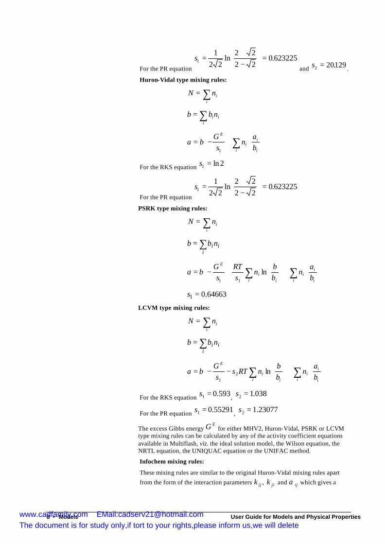
For the RKS equation s1 2= ln and s2 17 25= .
www.cadfamily.com EMail:[email protected] document is for study only,if tort to your rights,please inform us,we will delete
8 • Models User Guide for Models and Physical Properties
For the PR equation
s1
12 2
2 22 2
0 623225=+−
=ln .
and s2 20129= . .
Huron-Vidal type mixing rules:
N nii
= ∑
b b nii
i= ∑
a bGs
nab
E
ii
ii
= − +
∑
1
For the RKS equation s1 2= ln
For the PR equation
s1
12 2
2 22 2
0 623225=+−
=ln .
PSRK type mixing rules:
N nii
= ∑
ii
inbb ∑=
+
+−= ∑∑
i i
ii
i ii
E
ba
nbb
ns
RTs
Gba ln
11
64663.01 =s
LCVM type mixing rules:
N nii
= ∑
ii
inbb ∑=
+
−−= ∑∑
i i
ii
i ii
E
ba
nbb
nRTss
Gba ln2
1
For the RKS equation 593.01 =s , 038.12 =s
For the PR equation 55291.01 =s , 23077.12 =s
The excess Gibbs energy GE
for either MHV2, Huron-Vidal, PSRK or LCVM type mixing rules can be calculated by any of the activity coefficient equations available in Multiflash, viz. the ideal solution model, the Wilson equation, the NRTL equation, the UNIQUAC equation or the UNIFAC method.
Infochem mixing rules:
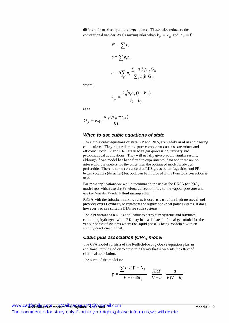
These mixing rules are similar to the original Huron-Vidal mixing rules apart
from the form of the interaction parameters ijk , jik and ijα which gives a
www.cadfamily.com EMail:[email protected] document is for study only,if tort to your rights,please inform us,we will delete
User Guide for Models and Physical Properties Models • 9
different form of temperature dependence. These rules reduce to the conventional van der Waals mixing rules when jiij kk = and 0=ijα .
N nii
= ∑
b b nii
i= ∑
a b nn b G
n b Gii
j j j ji ji
j j j ji
=∑
∑∑ξ
where:
ξ jii j ji
i j
a a k
b b=
−
+
2 1( )
and:
GRTji
ji ji ii=−
exp
( )α ξ ξ
When to use cubic equations of state The simple cubic equations of state, PR and RKS, are widely used in engineering calculations. They require limited pure component data and are robust and efficient. Both PR and RKS are used in gas-processing, refinery and petrochemical applications. They will usually give broadly similar results, although if one model has been fitted to experimental data and there are no interaction parameters for the other then the optimised model is always preferable. There is some evidence that RKS gives better fugacities and PR better volumes (densities) but both can be improved if the Peneloux correction is used.
For most applications we would recommend the use of the RKSA (or PRA) model sets which use the Peneloux correction, fit a to the vapour pressure and use the Van der Waals 1-fluid mixing rules.
RKSA with the Infochem mixing rules is used as part of the hydrate model and provides extra flexibility to represent the highly non-ideal polar systems. It does, however, require suitable BIPs for such systems.
The API variant of RKS is applicable to petroleum systems and mixtures containing hydrogen, while RK may be used instead of ideal gas model for the vapour phase of systems where the liquid phase is being modelled with an activity coefficient model.
Cubic plus association (CPA) model The CPA model consists of the Redlich-Kwong-Soave equation plus an additional term based on Wertheim’s theory that represents the effect of chemical association.
The form of the model is:
( )
)(45.0
1
bVVa
bVNRT
bV
XFnp
i
iiii
++
−+
−
−=
∑
www.cadfamily.com EMail:[email protected] document is for study only,if tort to your rights,please inform us,we will delete
10 • Models User Guide for Models and Physical Properties
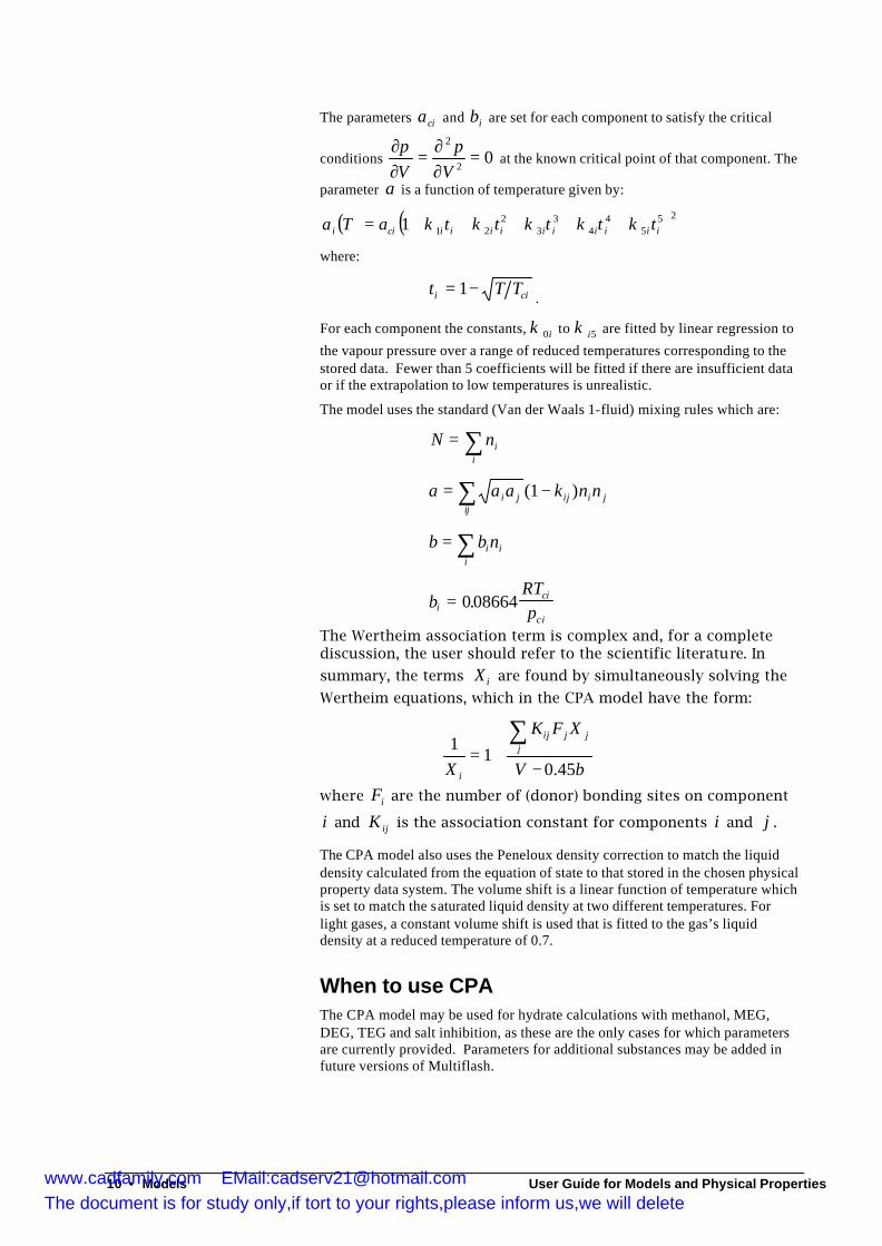
The parameters cia and ib are set for each component to satisfy the critical
conditions 02
2
=∂∂
=∂∂
Vp
Vp
at the known critical point of that component. The
parameter a is a function of temperature given by:
( ) ( )255
44
33
2211 iiiiiiiiiicii tttttaTa κκκκκ +++++=
where:
t T Ti ci= −1.
For each component the constants, i0κ to κ i5 are fitted by linear regression to
the vapour pressure over a range of reduced temperatures corresponding to the stored data. Fewer than 5 coefficients will be fitted if there are insufficient data or if the extrapolation to low temperatures is unrealistic.
The model uses the standard (Van der Waals 1-fluid) mixing rules which are:
N nii
= ∑
a a a k n ni jij
ij i j= −∑ ( )1
b b ni ii
= ∑
bRTpi
ci
ci= 0 08664.
The Wertheim association term is complex and, for a complete discussion, the user should refer to the scientific literature. In
summary, the terms iX are found by simultaneously solving the
Wertheim equations, which in the CPA model have the form:
bV
XFK
Xj
jjij
i 45.01
1−
+=∑
where iF are the number of (donor) bonding sites on component
i and ijK is the association constant for components i and j .
The CPA model also uses the Peneloux density correction to match the liquid density calculated from the equation of state to that stored in the chosen physical property data system. The volume shift is a linear function of temperature which is set to match the saturated liquid density at two different temperatures. For light gases, a constant volume shift is used that is fitted to the gas’s liquid density at a reduced temperature of 0.7.
When to use CPA The CPA model may be used for hydrate calculations with methanol, MEG, DEG, TEG and salt inhibition, as these are the only cases for which parameters are currently provided. Parameters for additional substances may be added in future versions of Multiflash.
www.cadfamily.com EMail:[email protected] document is for study only,if tort to your rights,please inform us,we will delete
User Guide for Models and Physical Properties Models • 11
PC-SAFT equation of state The PC-SAFT equation is a development of the SAFT model that has been shown to give good results for a wide range of polar and non-polar substances including polymers. Polymers are one of the most important areas of application of PC-SAFT. The model appears to be one of the most accurate and realistic equations of state currently available for modelling polymer systems.
PC-SAFT stands for the Perturbed Chain Statistical Associating Fluid Theory and it incorporates current ideas of how to model accurately the detailed thermodynamics of fluids within the framework of an equation of state. The mathematical structure is very complex and cannot be conveniently described in a manual. Users are referred to Appendix A of the reference given below.
Reference: Perturbed-Chain SAFT: An Equation of State Based on a Perturbation Theory for Chain Molecules by Gross and Sadowski in Industrial and Engineering Chemistry Research, 40, 1244, (2001).
The Multiflash version includes an implementation of the association term of PC-SAFT which is discussed in the paper, Application of the Perturbed-Chain SAFT Equation of State to Associating Systems by Gross and Sadowski in Industrial and Engineering Chemistry Research, 41, 5510, (2002). This paper however does not discuss the mathematical formulation of the association term; this can be found in the following reference.
Reference: New Reference Equation of State for Associating Liquids by Chapman, Gubbins, Jackson and Rodosz in Industrial and Engineering Chemistry Research, 29, 1709, (1990).
The Multiflash implementation follows the same general structure as the association term in the CPA model.
Multiflash also has a version of PC-SAFT with simplified mixing rules as proposed by researchers at the Danish Technical University.
Reference: Computational and Physical Performance of a Modified PC-SAFT Equation of State for Highly Asymmetric and Associating Mixtures by von Solms, Michelsen and Kontogeorgis in Industrial and Engineering Chemistry Research, 42, 1098, (2003).
Polymer Components Polymers are not well-defined chemical compounds but rather a distribution of chain molecules of varying molecular weight. In Multiflash, polymers must be represented by one or more pseudo components, which must be set up as user-defined components.
Using PC-SAFT, every pseudo component for a given polymer must be assigned the same values of the pure-compound parameters SAFTSIGMA (in metres, not Ångstrom units) and SAFTEK. In addition, the SAFTM parameter must be specified. This is normally quoted as a ratio to the molecular weight, so it has to be calculated for each polymer pseudo component knowing the molecular weight. For polystyrene, for example, Gross and Sadowski give the ratio as 0.019, so for a polystyrene pseudo component of molecular weight 100000, the SAFTM parameter should be set to 100000×0.019=1900, etc.
Additionally, the user can define association parameters if the polymer forms hydrogen bonds. These parameters are SAFTBETA which defines the volumetric or entropic parameter, and SAFTEPSILON the energy or enthalpy parameter. Multiflash also provides an extension to the PC-SAFT definition: the user can also supply a heat capacity parameter SAFTGAMMA for the association term. For the association term to be non-zero, the user must also define the parameter SAFTFF which denotes the number of donor bonding sites per segment of polymer.
www.cadfamily.com EMail:[email protected] document is for study only,if tort to your rights,please inform us,we will delete
12 • Models User Guide for Models and Physical Properties
Values of PC-SAFT parameters for polymers can be found in Modeling Polymer Systems Using the Perturbed-Chain Statistical Associating Fluid Theory Equation of State by Gross and Sadowski in Industrial and Engineering Chemistry Research, 41, 1084, (2002) and in Modeling of polymer phase equilibria using Perturbed-Chain SAFT by Tumakaka, Gross and Sadowski in Fluid Phase Equilibria, 194-197, 541, (2002).
Defining Polymers and Copolymers from their Segments Multiflash also allows the user to define up to four polymer segments which can be used to define any number of homopolymers or copolymers following the method of Tumakaka, Gross and Sadowski described in the reference above.
For each segment the user must define the molecular weight MW and the SAFT parameters SAFTEK and SAFTSIGMA. Optionally, the association parameters SAFTBETA, SAFTEPSILON, optionally SAFTGAMMA and SAFTFF can be defined.
Once a number of segments are defined, the user can then define polymers in terms of the segments as an alternative to the normal method of defining a SAFT component. To define polymer components in this manner, all the user has to do is define the molecular weight MW of the polymer and specify the bond fractions between the segments from which the polymer is constructed. If the polymer is formed from only one type of segment, it is a homopolymer of that segment; if it is formed of two or more types of segment, it is a copolymer. The definition of the bond fractions is given by Tumakaka, Gross and Sadowski, (although their examples of actual values of bond fractions are not realistic).
All other parameters of the polymer, including the segments fractions, are then internally calculated by Multiflash from the supplied molecular weight and bond fractions. The user can define the BIPs between normal components and/or segments. Note that in the fluid composition, the amounts of the segments must all be set to zero, as the segments are not real components of the mixture.
PSRK equation of state This model consists of the RKSA equation of state with vapour pressure fitting, the Peneloux volume correction and the PSRK type mixing rules. The excess Gibbs energy is provided by the PSRK variant of the Unifac method. This is the same as the normal VLE Unifac model except that the group table has been extended to include a large number of common light gases.
When to use PSRK The PSRK model is an extension of the Unifac method. It is intended to predict the phase behaviour of a wide range of polar mixtures using the solution of groups concept as embodied in Unifac. The main benefit of PSRK is that it is able to handle mixtures containing gases much better than Unifac and unlike a normal equation of state it can handle polar liquids. This is because (a) it uses an equation of state with an excess Gibbs energy mixing rule thereby avoiding problems of how to handle supercritical components in an activity coefficient equation; (b) the Unifac group parameter table has been extended in PSRK to include 32 common light gases.
LCVM equation of state This model consists of the PRA equation of state with vapour pressure fitting, the Peneloux volume correction and the LCVM type mixing rules. The excess Gibbs energy is provided by the LCVM variant of the Unifac method. This is the
www.cadfamily.com EMail:[email protected] document is for study only,if tort to your rights,please inform us,we will delete
User Guide for Models and Physical Properties Models • 13
same as the normal VLE Unifac model except that the group table has been extended to include a number of common light gases found in petroleum fluids.
When to use LCVM The LCVM model is an extension of the Unifac method. It is intended to predict the phase behaviour of petroleum fluids mixed with polar compounds using the solution of groups concept as embodied in Unifac. The main benefit of LCVM is that it is better able to handle asymmetric mixtures. This is because it uses an equation of state with an excess Gibbs energy mixing rule that was specifically designed to work with Unifac for mixtures of light gases and heavy hydrocarbons.
Lee-Kesler-Plöcker (LKP) equation of state The LKP method is a 3 parameter corresponding states method based on interpolating the reduced properties of a mixture between those of two reference substances. The equation for each property is of the form:
[ ]z z z zmix = + −( )( )
( ) ( )01
1 0ωω
The Multiflash implementation uses a single temperature independent interaction parameter.
When to use LKP The method predicts fugacity coefficients, thermal properties and volumetric properties of a mixture. However, it is rather slow and complex compared to the cubic equations of state and is not recommended for phase equilibrium calculations, although it can yield accurate predictions for density and enthalpy. It would normally be applied to non-polar or mildly polar mixtures such as hydrocarbons and light gases.
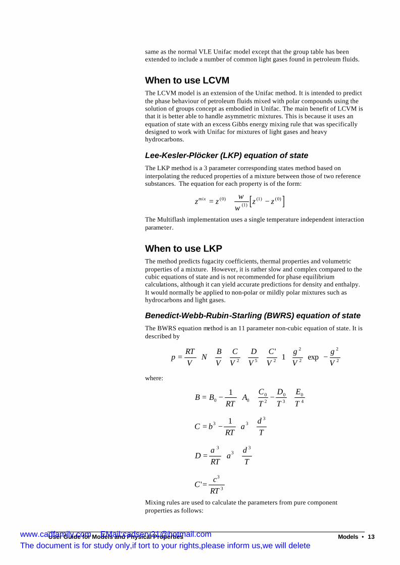
Benedict-Webb-Rubin-Starling (BWRS) equation of state The BWRS equation method is an 11 parameter non-cubic equation of state. It is described by
−
+++++= 2
2
2
2
252 exp1'
VVVC
VD
VC
VB
NVRT
pγγ
where:
+−+−=
40
30
20
001
TE
TD
TC
ART
BB
+−=
Td
aRT
bC3
33 1
+=
Td
aRT
D3
33α
3
3
'RTc
C =
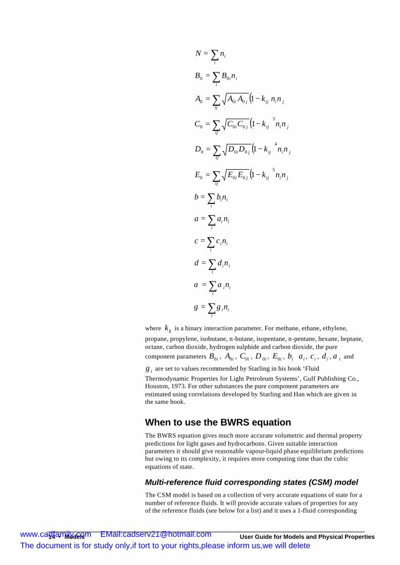
Mixing rules are used to calculate the parameters from pure component properties as follows:
www.cadfamily.com EMail:[email protected] document is for study only,if tort to your rights,please inform us,we will delete
14 • Models User Guide for Models and Physical Properties
N nii
= ∑
∑=i
iinBB 00
( ) jiij
ijji nnkAAA ∑ −= 1000
( ) jiij
ijji nnkCCC3
000 1∑ −=
( ) jiij
ijji nnkDDD4
000 1∑ −=
( ) jiij
ijji nnkEEE5
000 1∑ −=
b b ni ii
= ∑
∑=i
ii naa
∑=i
iincc
∑=i
iindd
∑=i
iinαα
∑=i
iinγγ
where k ij is a binary interaction parameter. For methane, ethane, ethylene,
propane, propylene, isobutane, n-butane, isopentane, n-pentane, hexane, heptane, octane, carbon dioxide, hydrogen sulphide and carbon dioxide, the pure component parameters iB0 , iA0 , iC0 , iD 0 , iE0 , ib ia , ic , id , iα and
iγ are set to values recommended by Starling in his book ‘Fluid
Thermodynamic Properties for Light Petroleum Systems’, Gulf Publishing Co., Houston, 1973. For other substances the pure component parameters are estimated using correlations developed by Starling and Han which are given in the same book.
When to use the BWRS equation The BWRS equation gives much more accurate volumetric and thermal property predictions for light gases and hydrocarbons. Given suitable interaction parameters it should give reasonable vapour-liquid phase equilibrium predictions but owing to its complexity, it requires more computing time than the cubic equations of state.
Multi-reference fluid corresponding states (CSM) model The CSM model is based on a collection of very accurate equations of state for a number of reference fluids. It will provide accurate values of properties for any of the reference fluids (see below for a list) and it uses a 1-fluid corresponding
www.cadfamily.com EMail:[email protected] document is for study only,if tort to your rights,please inform us,we will delete
User Guide for Models and Physical Properties Models • 15
states approach to estimate mixture properties. It is formulated so that mixture properties will reduce to the (accurate) pure component values as the mixture composition approaches each of the pure component limits.
The model definition can be considered in two distinct parts: the definition of pseudo-critical properties for a mixture (mixing rules), and the prescription for combining the properties of the reference substances to give the total mixture properties (combining rules).
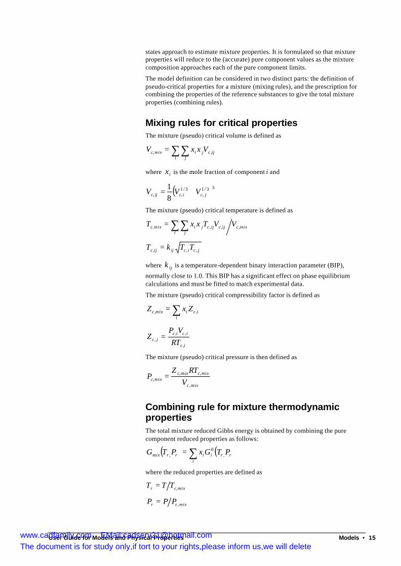
Mixing rules for critical properties The mixture (pseudo) critical volume is defined as
∑∑=i j
ijcjimixc VxxV ,,
where ix is the mole fraction of component i and
( )33/1,
3/1,, 8
1jcicijc VVV +=
The mixture (pseudo) critical temperature is defined as
mixci j
ijcijcjimixc VVTxxT ,,,. ∑∑=
jcicijijc TTkT ,,, =
where ijk is a temperature-dependent binary interaction parameter (BIP),
normally close to 1.0. This BIP has a significant effect on phase equilibrium calculations and must be fitted to match experimental data.
The mixture (pseudo) critical compressibility factor is defined as
∑=i
icimixc ZxZ ,,
ic
icicjc RT
VPZ
,
,,, =
The mixture (pseudo) critical pressure is then defined as
mixc
mixcmixcmixc V
RTZP
,
,,, =
Combining rule for mixture thermodynamic properties The total mixture reduced Gibbs energy is obtained by combining the pure component reduced properties as follows:
( ) ( )∑=i
rriirrmix PTGxPTG ,0
,
where the reduced properties are defined as
mixcr TTT ,=
mixcr PPP ,=
www.cadfamily.com EMail:[email protected] document is for study only,if tort to your rights,please inform us,we will delete
16 • Models User Guide for Models and Physical Properties
All other thermodynamic properties are obtained from the Gibbs energy by differentiation.
IAPWS-95 The reference equation of state used for water is the IAPWS-95 scientific formulation. It is also available as a separate model option. For water the recommended equations for transport properties have also been implemented.
Reference fluids The current model implementation includes reference equations of state for the following substances: argon, iso-butane, n-butane, CO, CO2 , ethane, ethylene, fluorine, H2S, hydrogen, methane, nitrogen, octane, oxygen, n-pentane, propane, water (IAPSW 95), xenon, helium, hexane, heptane, octane, ammonia, neon, propylene, R123, R152a, R124, R125, R134a, R22, R32, R11, R113, R114, R115, R116, R12, R13, R14, R23, and RC318. Hydrocarbons between pentane and octane are modelled as combinations of these substances. The equations of state are taken fro m various sources and do not all have the same quality or range of applicability.
Applicability The model is very accurate for pure substances that are included in the above list of reference substances. It is also applicable to near-ideal mixtures such as air but for the best results it is necessary to fit values of the binary interaction parameters to match experimental data. The model should not be used for non-ideal mixtures such as water + CO2 etc.
Activity coefficient methods In an ideal liquid solution the liquid fugacity of each component in the mixture is directly proportional to the mole fraction of the component
f x fil
i il= *,
The ideal solution assumes that all molecules in the liquid solution are identical in size and are randomly distributed. This assumption is valid for mixtures made up of molecules of similar size and type, but for mixtures of unlike molecules you must expect varying degrees of non-ideality. The activity coefficient, γ i , represents the deviation of the mixture from ideality, as defined by the ideal solution.
The fugacity coefficients for the activity coefficient equations are calculated from the standard relationship:
ln ln ln ln lnϕ γ ϕi i isat
isat
ip p= + + − + Π
where γ i is the activity coefficient of component i which is derived from the excess Gibbs energy as follows:
lnγ∂∂i
E
i
Gn
=
.
pisat is the saturated vapour pressure of component i ,ϕ i
sat is the fugacity
coefficient of the pure saturated vapour of component i (calculated from the gas phase model associated with the activity coefficient equation) and p is the total pressure.
www.cadfamily.com EMail:[email protected] document is for study only,if tort to your rights,please inform us,we will delete
User Guide for Models and Physical Properties Models • 17
The Poynting correction, Π i , corrects the fugacity coefficient from the standard state pressure (i.e. the saturation pressure) to the system pressure. It is evaluated on the assumption of ideality, i.e. assuming that there is zero excess volume of mixing, and that the liquid is incompressible:
Π iisat
isatp p v
RT=
−( )
where visat is the saturated liquid volume of component i .
Activity coefficient equations in Multiflash A number of activity coefficient equations are available in Multiflash and are described below. The nomenclature is to denote binary interaction parameters between components i and j by Aij . The NRTL equation has an additional
parameterα ij .
Ideal solution model This is described by:
GRT
E
= 0
The ideal solution model may be used when the mixture is ideal, i.e. when there are no mixing effects. It an also be used for single components to calculate some pure component properties from the physical property databank.
Wilson E equation This is defined by:
GRT
nG n
n
E
ij ij j
j ji
=∑
∑
∑ ln
where:
GV
V
A
RTijj
i
ij= −
*
* exp
Vi* is the saturated liquid molar volume of component i (extrapolated in the
case of supercritical gases) evaluated at a fixed reference temperature of 298.15K.
This model may be used for vapour-liquid equilibrium calculations but it is not capable of predicting liquid-liquid immiscibility. Binary interaction parameters are provided in our INFOBIPS bank for some component pairs. If no BIPs are included for your particular mixture then to obtain accurate predictions you must supply binary interaction parameter values in the correct units.
Wilson A equation
GRT
nA n
n
E
ij ij j
j ji
=∑
∑
∑ ln
This model which is a simplified form of the Wilson E model, may be used for vapour-liquid equilibrium calculations but it is not capable of predicting liquid-
www.cadfamily.com EMail:[email protected] document is for study only,if tort to your rights,please inform us,we will delete
18 • Models User Guide for Models and Physical Properties
liquid immiscibility. To obtain accurate predictions you must supply binary interaction parameters (BIP) values, which are dimensionless.
NRTL equation
GRT
nA G n
n G
E
ij ij ji j
j j jii
=∑
∑
∑ ln
where:
Ga A
RTijij ij= −
exp
The NRTL model may be used for vapour-liquid, liquid-liquid and vapour-liquid -liquid calculations (the VLE option should be used for VLLE). Again if BIP values are not provided in INFOBIPS they must be supplied for accurate predictions. In cases where the user does not specify any value for the non-randomness factor,α ij , it is automatically set to 0.3 if the VLE version of NRTL
is specified or to 0.2 if the LLE version is specified. Note that α αij ji= so
only α ij need be supplied.
UNIQUAC equation
∑ ∑∑
∑ ∑∑
∑ ∑∑
+
+
=i
jjj
jjjji
iii
jjji
jjji
iii
jjj
jji
i
E
nq
nqGnq
nqr
nrqnq
znr
nrn
RTG
lnln2
ln
where:
z = 10
and:
GA
RTijij= −
exp
The UNIQUAC model may be used for vapour-liquid, liquid-liquid and vapour-liquid -liquid calculations. In Multiflash we provide UNIQUAC VLE and LLE variants as for the NRTL equation. Again BIP values must be supplied for accurate predictions if they are not included in INFOBIPS. For VLLE the variant chosen should be guided by the BIPs available.
Original UNIFAC method The UNIFAC method is similar to UNIQUAC but the interaction parameters are predicted based on the molecular group structure of the components in the mixture. The is completely predictive and does not require the user to supply BIPs.
∑∑ ∑
∑∑ ∑
∑−+
+
=i
(i)
ii
jjji
jjji
iii
jjj
jji
i
E
RTn
RTnqr
nrqnq
znr
nrn
RTG GG
ln2
ln
where iq and ir are the UNIQUAC/UNIFAC surface and volume parameters
for component i and 10=z . For UNIFAC they are found by summing the contributions from the groups from which each component is formed. G is the
www.cadfamily.com EMail:[email protected] document is for study only,if tort to your rights,please inform us,we will delete
User Guide for Models and Physical Properties Models • 19
residual excess Gibbs energy of the solution and )(iG is the residual excess
Gibbs energy of pure component i according to the principle of solution of groups. The UNIFAC residual term is given by:
∑ ∑∑
Ψ−=
kl
ll
ll
llk
kk NQ
NQQN
RTln
G
The summation is over all groups in the mixture (or pure component). kN is the
total number of moles of group k , kQ is the surface area parameter for group
k and lkΨ is the interaction parameter:
−=Ψ
RTAlk
lk exp
In original UNIFAC, the two binary parameters lkA between components l and
k are normally taken as constants.
Dortmund modified UNIFAC method
∑∑ ∑∑
∑ ∑∑
−+
+
=
i
(i)
ii
jjji
jjji
iii
jjj
jji
i
E
RTn
RTnqr
nrqnq
znr
nrn
RTG GG
ln2
ln 4/3
4/3
where iq and ir are the UNIQUAC/UNIFAC surface and volume parameters
for component i and 10=z . For UNIFAC they are found by summing the contributions from the groups from which each component is formed. G is the
residual excess Gibbs energy of the solution and )(iG is the residual excess
Gibbs energy of pure component i according to the principle of solution of groups. The UNIFAC residual term is given by:
∑ ∑∑
Ψ−=
kl
ll
ll
llk
kk NQ
NQQN
RTln
G
The summation is over all groups in the mixture (or pure component). kN is the
total number of moles of group k , kQ is the surface area parameter for group
k and lkΨ is the interaction parameter:
−=Ψ
RTAlk
lk exp
For Dortmund modified UNIFAC, the two binary parameters lkA between
components l and k are treated as quadratic functions of temperature.
Dortmund modified UNIFAC is better able to represent the simultaneous vapour-liquid equilibria, liquid-liquid equilibria and excess enthalpies of polar mixtures than the original UNIFAC method. Like original UNIFAC, however, it does not allow for the presence of light gases in the mixture.
www.cadfamily.com EMail:[email protected] document is for study only,if tort to your rights,please inform us,we will delete
20 • Models User Guide for Models and Physical Properties
References: Gmehling and co-workers, A Modified UNIFAC Model. 1. Prediction of VLE, hE, and γ∞, Industrial and Engineering Chemistry Research, 26, 1372, (1987); A Modified UNIFAC Model. 2. Present Parameter Matrix and Results for Different Thermodynamic Properties, ibid., 32, 178, (1993); A Modified UNIFAC (Dortmund) Model. 3. Revision and Extension , ibid., 37, 4876, (1998); A Modified UNIFAC (Dortmund) Model. 4. Revision and Extension, ibid., 41, 1678, (2002).
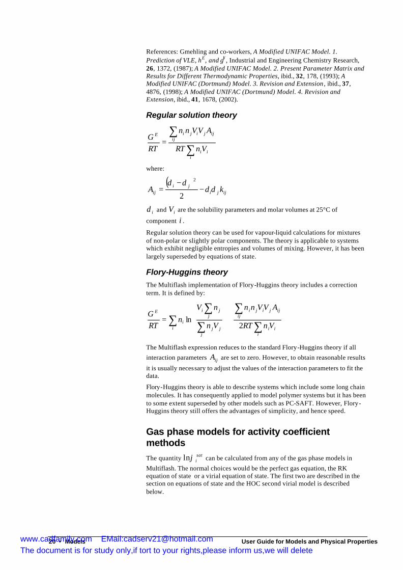
Regular solution theory
∑
∑=
iii
ijijjijiE
VnRT
AVVnn
RTG
where:
( )ijji
jiij kA δδ
δδ−
−=
2
2
iδ and iV are the solubility parameters and molar volumes at 25°C of
component i .
Regular solution theory can be used for vapour-liquid calculations for mixtures of non-polar or slightly polar components. The theory is applicable to systems which exhibit negligible entropies and volumes of mixing. However, it has been largely superseded by equations of state.
Flory-Huggins theory The Multiflash implementation of Flory-Huggins theory includes a correction term. It is defined by:
∑
∑∑ ∑
∑+
=
iii
ijijjiji
ij
jj
jji
i
E
VnRT
AVVnn
Vn
nVn
RTG
2ln
The Multiflash expression reduces to the standard Flory-Huggins theory if all
interaction parameters ijA are set to zero. However, to obtain reasonable results
it is usually necessary to adjust the values of the interaction parameters to fit the data.
Flory-Huggins theory is able to describe systems which include some long chain molecules. It has consequently applied to model polymer systems but it has been to some extent superseded by other models such as PC-SAFT. However, Flory-Huggins theory still offers the advantages of simplicity, and hence speed.
Gas phase models for activity coefficient methods The quantity lnϕi
sat can be calculated from any of the gas phase models in
Multiflash. The normal choices would be the perfect gas equation, the RK equation of state or a virial equation of state. The first two are described in the section on equations of state and the HOC second virial model is described below.
www.cadfamily.com EMail:[email protected] document is for study only,if tort to your rights,please inform us,we will delete
User Guide for Models and Physical Properties Models • 21
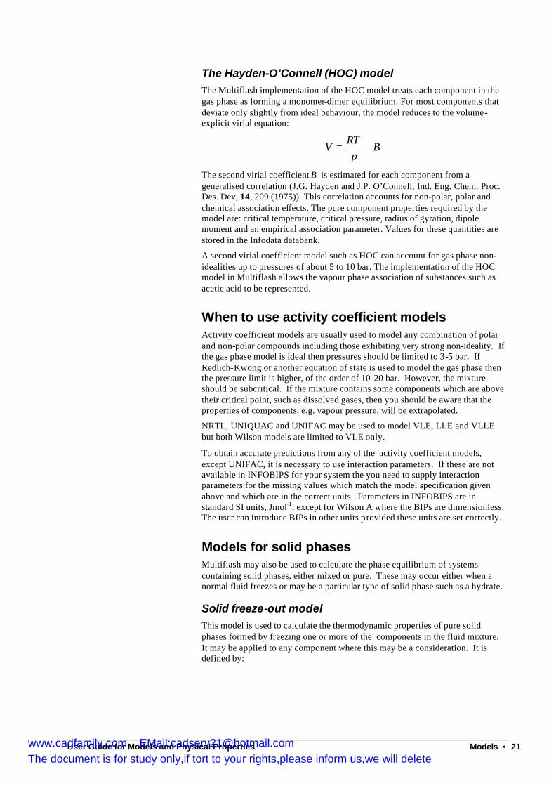
The Hayden-O’Connell (HOC) model The Multiflash implementation of the HOC model treats each component in the gas phase as forming a monomer-dimer equilibrium. For most components that deviate only slightly from ideal behaviour, the model reduces to the volume-explicit virial equation:
Bp
RTV +=
The second virial coefficient B is estimated for each component from a generalised correlation (J.G. Hayden and J.P. O’Connell, Ind. Eng. Chem. Proc. Des. Dev, 14, 209 (1975)). This correlation accounts for non-polar, polar and chemical association effects. The pure component properties required by the model are: critical temperature, critical pressure, radius of gyration, dipole moment and an empirical association parameter. Values for these quantities are stored in the Infodata databank.
A second virial coefficient model such as HOC can account for gas phase non-idealities up to pressures of about 5 to 10 bar. The implementation of the HOC model in Multiflash allows the vapour phase association of substances such as acetic acid to be represented.
When to use activity coefficient models Activity coefficient models are usually used to model any combination of polar and non-polar compounds including those exhibiting very strong non-ideality. If the gas phase model is ideal then pressures should be limited to 3-5 bar. If Redlich-Kwong or another equation of state is used to model the gas phase then the pressure limit is higher, of the order of 10-20 bar. However, the mixture should be subcritical. If the mixture contains some components which are above their critical point, such as dissolved gases, then you should be aware that the properties of components, e.g. vapour pressure, will be extrapolated.
NRTL, UNIQUAC and UNIFAC may be used to model VLE, LLE and VLLE but both Wilson models are limited to VLE only.
To obtain accurate predictions from any of the activity coefficient models, except UNIFAC, it is necessary to use interaction parameters. If these are not available in INFOBIPS for your system the you need to supply interaction parameters for the missing values which match the model specification given above and which are in the correct units. Parameters in INFOBIPS are in standard SI units, Jmol-1, except for Wilson A where the BIPs are dimensionless. The user can introduce BIPs in other units provided these units are set correctly.
Models for solid phases Multiflash may also be used to calculate the phase equilibrium of systems containing solid phases, either mixed or pure. These may occur either when a normal fluid freezes or may be a particular type of solid phase such as a hydrate.
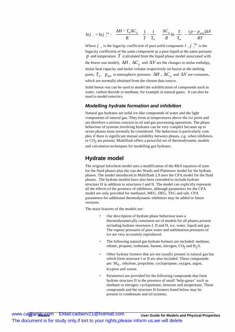
Solid freeze-out model This model is used to calculate the thermodynamic properties of pure solid phases formed by freezing one or more of the components in the fluid mixture. It may be applied to any component where this may be a consideration. It is defined by:
www.cadfamily.com EMail:[email protected] document is for study only,if tort to your rights,please inform us,we will delete
22 • Models User Guide for Models and Physical Properties
ln ln ln( )
ϕ ϕi iliq m p
m
p
m
atmH T C
R T T
C
RTT
p p VRT
= −−
−
+
−
−∆ ∆ ∆ ∆1 1
Where ϕ i is the fugacity coefficient of pure solid component i , ϕ iliq is the
fugacity coefficient of the same component as a pure liquid at the same pressure p and temperature T (calculated from the liquid phase model associated with
the freeze -out model), ∆H , ∆Cp and ∆V are the changes in molar enthalpy,
molar heat capacity and molar volume respectively on fusion at the melting point, Tm . patm is atmospheric pressure. ∆H , ∆Cp and ∆V are constants,
which are normally obtained from the chosen data source.
Solid freeze -out can be used to model the solidification of compounds such as water, carbon dioxide or methane, for example in natural gases. It can also be used to model eutectics.
Modelling hydrate formation and inhibition Natural gas hydrates are solid ice-like compounds of water and the light components of natural gas. They form at temperatures above the ice point and are therefore a serious concern in oil and gas processing operations. The phase behaviour of systems involving hydrates can be very complex because up to seven phases must normally be considered. The behaviour is particularly com-plex if there is significant mutual solubility between phases, e.g. when inhibitors or CO2 are present. Multiflash offers a powerful set of thermodynamic models and calculation techniques for modelling gas hydrates.
Hydrate model The original Infochem model uses a modification of the RKS equation of state for the fluid phases plus the van der Waals and Platteeuw model for the hydrate phases. The model introduced in Multiflash 2.9 uses the CPA model for the fluid phases. The hydrate models have also been extended to include hydrate structure H in addition to structures I and II. The model can explicitly represent all the effects of the presence of inhibitors, although parameters for the CPA model are only provided for methanol, MEG, DEG, TEG and salt. CPA parameters for additional thermodynamic inhibitors may be added in future versions.
The main features of the models are:
• Our description of hydrate phase behaviour uses a thermodynamically consistent set of models for all phases present including hydrate structures I, II and H, ice, water, liquid and gas. The vapour pressures of pure water and sublimation pressures of ice are very accurately reproduced.
• The following natural gas hydrate formers are included: methane, ethane, propane, isobutane, butane, nitrogen, CO2 and H2S.
• Other hydrate formers that are not usually present in natural gas but which form structure I or II are also included. These compounds are: SF6 , ethylene, propylene, cyclopropane, oxygen, argon, krypton and xenon.
• Parameters are provided for the following compounds that form hydrate structure II in the presence of small ‘help-gases’ such as methane or nitrogen: cyclopentane, benzene and neopentane. These compounds and the structure H formers listed below may be present in condensate and oil systems.
www.cadfamily.com EMail:[email protected] document is for study only,if tort to your rights,please inform us,we will delete
User Guide for Models and Physical Properties Models • 23
• Structure H hydrates form in the presence of small ‘help-gases’ such as methane or nitrogen but the formation temperatures are significantly higher (about 10 K) than pure methane or nitrogen hydrate. In practice it seems that structure II hydrates form before structure H but if there is enough water structure H may be formed too. The structure H model includes parameters for:
isopentane neohexane 2,3-dimethylbutane 2,2,3-trimethylbutane 2,2-dimethylpentane 3,3-dimethylpentane methylcyclopentane methylcyclohexane cis -1,2-dimethylcyclohexane 2,3-dimethyl-1-butene 3,3-dimethyl-1-butene cycloheptene cis -cyclooctene adamantane ethylcyclopentane 1,1-dimethylcyclohexane ethylcyclohexane cyclohexane cycloheptane cyclooctane
• The thermal properties (enthalpies and entropies) of the hydrates and ice are included permitting isenthalpic and isentropic flashes involving these phases.
• Calculations can be made for any possible combination of phases including cases without free water. No modification of the phase models is required to do this.
• The properties of the hydrates have been fixed by investigating data for natural gas components in both simple and mixed hydrates to obtain reliable predictions of structure I, structure II and structure H hydrates.
• The properties of the empty hydrate lattices have been investigated and the most reliable values have been adopted.
• Proper allowance has been made for the solubilities of the gases in water so that the model parameters are not distorted by this effect. This is particularly important for carbon dioxide and hydrogen sulphide which are relatively soluble in water.
• Correct thermodynamic calculations of the most stable hydrate structure have been made.
The model is used to calculate the hydrate equilibrium formation temperature at a given pressure or pressure at a given temperature where the first very small quantity of hydrate appears after a sufficiently long time. This point corresponds to the thermodynamic formation point, also known as the hydrate dissociation point. Before the thermodynamic formation point is reached hydrate cannot form - this point is also called the stability limit. Beyond the stability limit hydrate can form but may not do so for a long time.
The model has been tested on a wide selection of open literature and proprietary experimental data. In most cases the hydrate dissociation temperature is predicted to within 1K.
www.cadfamily.com EMail:[email protected] document is for study only,if tort to your rights,please inform us,we will delete
24 • Models User Guide for Models and Physical Properties
Hydrates in water sub-saturated systems Hydrates can form even in systems where there is no free water present. Our hydrate model, with both RKSAINFO and CPA used to model the fluid phase, is capable of modelling this, although the data available for validating the results are very limited. What we have noticed is that for systems with very little water and at high pressures the predicted hydrate dissociation temperatures using RKSAINFO and CPA tend to diverge with increasing pressure, with CPA predicting lower hydrate dissociation temperatures than RKSAINFO. There are no data presently available to confirm which is correct. If this causes any difficulty it is possible to reproduce the CPA predictions with RKSAINFO by using parameters which reduce the Infochem mixing rule to van der Waals. These parameters, for methane, ethane and propane with water, are stored in the file vdwbip.mfc. They can be used to overwrite the existing BIPs for these binaries by loading this file after you have defined the hydrate model based on RKSAINFO as the fluid model.
When compared to the available data all three possible variants (CPA, RKSAINFO with standard and vdw BIP) give hydrate dissociation results within experimental error.
Nucleation model The nucleation model was developed in collaboration with BP as part of the EUCHARIS joint venture. This model is an extension of the existing thermodynamic model for hydrates described above. In order to extend the nucleation model into the Multiflash program, the following enhancements to the nucleation model were made:
• The model was extended to cover the homogeneous nucleation of ice and fitted to available ice nucleation data.
• The model was generalised to cover in principle nucleation from any liquid or gas phase.
• A correction for heterogeneous nucleation was included that was matched to available hydrate nucleation data.
• An improved expression was adopted for fluid diffusion rates.
• More robust numerical methods were introduced into the program.
The nucleation model provides an estimate of the temperature or pressure at which hydrates can be realistically expected to form. The model is based on the statistical theory of nucleation in multicomponent systems. Although there are limitations and approximations involved in this approach it has the major benefit that a practical nucleation model can be incorporated within the framework of a traditional thermodynamic hydrate modelling package.
Many of the comparisons of model predictions with experimental data have been made. In general measurements of hydrate nucleation result in an experimental error of ± 2ºC and predictions are usually within this error band.
With the existing Infochem hydrate model and the nucleation model, the hydrate formation and dis sociation boundaries can be predicted between which is the hydrate formation risk area.
Inhibitor modelling Thermodynamic hydrate inhibitors decrease the temperature or increase the pressure at which hydrates will form from a given gas mixture. The original Infochem hydrate model includes parameters for the commonly used inhibitors: methanol, salts, and the glycols MEG, DEG and TEG and for the less well-tested inhibitors ethanol, iso-propanol, propylene glycol and glycerol. A new mixing
www.cadfamily.com EMail:[email protected] document is for study only,if tort to your rights,please inform us,we will delete
User Guide for Models and Physical Properties Models • 25
rule was developed for the SRK equation of state to model the effects of the inhibitors on the fluid phases.
The hydrate model using CPA to model the fluid phases is limited in the current version of Multiflash to hydrate calculations with pure water or with methanol, MEG, DEG, TEG and salt. Additional parameters to extend the CPA model to cover the full range of thermodynamic inhibitors listed above will be included in future versions.
The treatment of hydrate inhibition has the following features:
• The model can explicitly represent all the effects of inhibitors including the depression of the hydrate formation temperature, the depression of the freezing point of water, the reduction in the vapour pressure of water (i.e. the dehydrating effect) and the partitioning of water and inhibitor between the oil, gas and aqueous phases.
• The model has been developed using all available data for mixtures of water with methanol, MEG, DEG and TEG. This involves representing simultaneously hydrate dissociation temperatures, depression of freezing point data and vapour-liquid equilibrium data.
• Two salt inhibition models are available. The older model is based on a salt component. The new model is a (restricted) electrolyte model. A salinity calculator tool is provided which allows the salt composition to be entered in a variety of units and calculates the equivalent amount of sodium chloride in the mixture. The equivalent composition is based on the freezing point depression and hydrate inhibition effect of the salts.
• The solubilities of hydrocarbons and light gases in water/inhibitor mixtures have also been represented.
Salinity Model Both salinity models operate at present on a sodium chloride equivalent basis. The salt component model represents the effect of sodium chloride in aqueous solution by a special equation of state component called “salt component” or “saltcomp”. This model is designed to operate with the Advanced RKS equation although it is also usable with the Advanced PR equation. The salt component model cannot be used with the CPA model or any other equation of state.
The new electrolyte model is designed to be added on to any equation of state. The models selection form allows it to be selected for use with the Advanced RKS equation and the CPA model. It represents sodium chloride as a equimolar combination of sodium and chloride ions. Future versions of Multiflash will extend this to other ions.
Modelling wax deposition Waxes are complex mixtures of solid hydrocarbons that freeze out of crude oils if the temperature is low enough. Under conditions of interest to the oil industry, waxes consist mainly of normal paraffins. Waxes are thought to consist of many crystals each of which is a solid solution of n-paraffins of a fairly narrow range in molecular weight.
Multiflash contains two wax models, the Coutinho model and the multisolid model. The features of the Coutinho model are:
The Coutinho model represents wax as a solid solution. There are two versions of the model, the Wilson and Uniquac variants. The version normally selected in Multiflash is the Wilson model which approximates the wax as a single solid
www.cadfamily.com EMail:[email protected] document is for study only,if tort to your rights,please inform us,we will delete
26 • Models User Guide for Models and Physical Properties
solution. This approach is relatively simple to apply and gives a good representation of the data, so it is recommended for general engineering use. The more complex Uniquac variant models the tendency of waxes to split into several separate solid solution phases. The Uniquac variant can be activated by configuration files that can be supplied by Infochem for users who wish to simulate the detailed physical chemistry of wax precipitation.
The model gives good predictions of waxing behaviour, both wax appearance temperature and the amount of wax precipitated at different temperatures. The method is applicable to both live and dead oils.
The model requires that the normal paraffins are explicitly present in the fluid model, as these are the wax forming components. The user must therefore use the new characterisation method either to enter the measured n-paraffin concentrations or else to estimate the n-paraffin distribution. The composition of the wax phase is determined by the known thermal properties (normal melting point, enthalpy of fusion, etc.) of the n-paraffins combined with their solution behaviour in both oil and wax phases.
In principle the wax model can be used in conjunction with any conventional cubic equations of state. The default options in the Multiflash implementation is RKSA.
The multisolid wax model is still available as an alternative option. The features of this model are:
It approximates waxing behaviour by representing the wax as a mixture of separate phases, each one of which corresponds to a pure pseudo component from the equation of state model. The composition of the wax phase is determined by the assumed thermodynamic properties (normal melting point, enthalpy of fusion, etc.) for the petroleum fractions heavier than C6 but which are not asphaltenes and resins.
The multisolid wax model should be used in conjunction with conventional cubic equations of state. The default option from the usual model set selection is RKSA but the multisolid model with PRA may be accessed from the waxpra.mfc file.
The original Infochem oil characterisation method should be used in conjunction with the multisolid wax model, as the model was set up to be compatible with this method. We recommend that the oil should be represented by 15 pseudo components and the RKSA model should be selected.
Modelling asphaltene flocculation Asphaltenes are polar compounds that are stabilised in crude oil by the presence of resins. If the oil is diluted by light hydrocarbons, the concentration of resins goes down and a point may be reached where the asphaltene is no longer stabilised and it flocculates to form a solid deposit. Because the stabilising action of the resins works through the mechanism of polar interactions, their effect becomes weaker as the temperature rises, i.e. flocculation may occur as the temperature increases. However, as the temperature increases further the asphaltene becomes more soluble in the oil. Thus, depending on the temperature and the composition of the oil, it is possible to find cases where flocculation both increases and decreases with increasing temperature.
The asphaltene model is based on the RKS cubic equation of state with addi-tional terms to describe the association of asphaltene molecules and their solvation by resin molecules. The interactions between asphaltenes and asphaltenes -resins are characterised by two temperature-dependent association constants: AAK and ARK . The remaining components are described by the van
der Waals 1-fluid mixing rule with the usual binary in teraction parameters ijk so
the asphaltene model is completely compatible with existing engineering
www.cadfamily.com EMail:[email protected] document is for study only,if tort to your rights,please inform us,we will delete
User Guide for Models and Physical Properties Models • 27
approaches that are adequate for describing vapour-liquid equilibria. The model is a comp utationally-efficient way of in corporating complex chemical effects into a cubic equation of state.
Other thermodynamic models Multiflash also incorporates a corresponding states method for estimating the density of liquid mixtures, the COSTALD model.
COSTALD liquid density model The volume of a liquid on the saturation line is defined by:
[ ]VV
V Vsat
R R*( ) ( )= −0 11 ω
where V sat is the saturated liquid volume, V * is a characteristic volume for
each substance, ω is the acentric factor and VR( )0 and VR
( )1 are generalised
functions of reduced temperature. In the Infochem implementation V * is obtained by matching the saturated liquid volume stored in the databank at 298 K or a reduced temperature of 0.7, whichever is the lower.
The volume of a compressed liquid is given by:
VV
CB p
B psat sat= −′ +
′ +
1 ln
where ′B is a generalised function of reduced temperature and ω , C is a
generalised function of ω , and p sat is the saturation pressure at the given temperature.
The COSTALD method can provide very accurate volumes for pure substances and simple mixtures, such as LNG. It is valid for liquids on the saturation line and compressed liquids up to a reduced temperature of 0.9. It is not necessarily accurate for heavy hydrocarbon mixtures with dissolved gases.
Transport property models For each of the transport properties, viscosity, thermal conductivity and surface tension, Multiflash offers two approaches to obtaining values for mixtures. One route is to calculate the property for a mixture by combining the property values for the pure components of which it is composed; the mixing rule approach. The other is to use a predictive method suitable for the property in question.
Viscosity
Pedersen Model This is a predictive corresponding states model originally developed for oil and gas systems. It is based on accurate correlations for the viscosity and density of the reference substance which is methane. The model is applicable to both gas and liquid phases. The Infochem implementation of the Pedersen model includes modifications to ensure that the viscosity of liquid water, methanol, ethanol, MEG, DEG and TEG and aqueous solutions of these components or salt are predicted reasonably well. We would recommend this method for oil and gas applications. It is the default viscosity model for use with equations of state.
www.cadfamily.com EMail:[email protected] document is for study only,if tort to your rights,please inform us,we will delete
28 • Models User Guide for Models and Physical Properties
Reference: Pedersen, Fredenslund and Thomassen, Properties of Oils and Natural Gases, Gulf Publishing Co., (1989).
Twu Model This is a predictive model suitable for oils. It is based on a correlation of the API nomograph for kinematic viscosity plus a mixing rule for blending oils. It is only applicable to liquids.
Reference: Twu, Generalised method for predicting viscosities of petroleum fractions, AIChE Journal, 32, 2091, (1986).
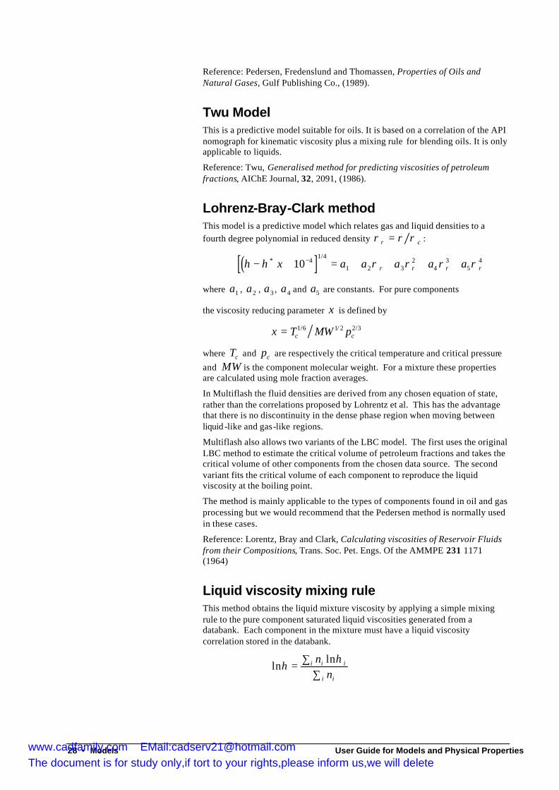
Lohrenz-Bray-Clark method This model is a predictive model which relates gas and liquid densities to a fourth degree polynomial in reduced density ρ ρ ρr c= :
( )[ ]η η ξ ρ ρ ρ ρ− + = + + + +−*/
10 41 4
1 2 32
43
54a a a a ar r r r
where a1 , a2 , a3 , a4 and a5 are constants. For pure components
the viscosity reducing parameter ξ is defined by
ξ = T MW pc c1 6 1 2 2 3/ / /
where Tc and pc are respectively the critical temperature and critical pressure
and MW is the component molecular weight. For a mixture these properties are calculated using mole fraction averages.
In Multiflash the fluid densities are derived from any chosen equation of state, rather than the correlations proposed by Lohrentz et al. This has the advantage that there is no discontinuity in the dense phase region when moving between liquid -like and gas-like regions.
Multiflash also allows two variants of the LBC model. The first uses the original LBC method to estimate the critical volume of petroleum fractions and takes the critical volume of other components from the chosen data source. The second variant fits the critical volume of each component to reproduce the liquid viscosity at the boiling point.
The method is mainly applicable to the types of components found in oil and gas processing but we would recommend that the Pedersen method is normally used in these cases.
Reference: Lorentz, Bray and Clark, Calculating viscosities of Reservoir Fluids from their Compositions, Trans. Soc. Pet. Engs. Of the AMMPE 231 1171 (1964)
Liquid viscosity mixing rule This method obtains the liquid mixture viscosity by applying a simple mixing rule to the pure component saturated liquid viscosities generated from a databank. Each component in the mixture must have a liquid viscosity correlation stored in the databank.
lnln
ηη
=∑
∑i i i
i i
nn
www.cadfamily.com EMail:[email protected] document is for study only,if tort to your rights,please inform us,we will delete
User Guide for Models and Physical Properties Models • 29
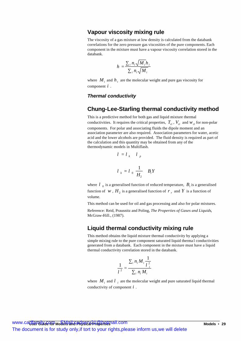
Vapour viscosity mixing rule The viscosity of a gas mixture at low density is calculated from the databank correlations for the zero pressure gas viscosities of the pure components. Each component in the mixture must have a vapour viscosity correlation stored in the databank.
ηη
=∑
∑i i i i
i i i
n M
n M
where M i and ηi are the molecular weight and pure gas viscosity for
component i .
Thermal conductivity
Chung-Lee-Starling thermal conductivity method This is a predictive method for both gas and liquid mixture thermal conductivities. It requires the critical properties, Tci , Vci and ωci for non-polar components. For polar and associating fluids the dipole moment and an association parameter are also required. Association parameters for water, acetic acid and the lower alcohols are provided. The fluid density is required as part of the calculation and this quantity may be obtained from any of the thermodynamic models in Multiflash.
λ λ λκ= + p
λ λκ = +
0
2
1H
B Yi
where λ 0 is a generalised function of reduced temperature, Bi is a generalised
function of ω , H 2 is a generalised function of ρ r and Y is a function of volume.
This method can be used for oil and gas processing and also for polar mixtures.
Reference: Reid, Prausnitz and Poling, The Properties of Gases and Liquids, McGraw-Hill., (1987).
Liquid thermal conductivity mixing rule This method obtains the liquid mixture thermal conductivity by applying a simple mixing rule to the pure component saturated liquid therma l conductivities generated from a databank. Each component in the mixture must have a liquid thermal conductivity correlation stored in the databank.
11
2
2
λλ
=∑
∑
i i ii
i i i
n M
n M
where M i and λ i are the molecular weight and pure saturated liquid thermal
conductivity of component i .
www.cadfamily.com EMail:[email protected] document is for study only,if tort to your rights,please inform us,we will delete
30 • Models User Guide for Models and Physical Properties
Vapour thermal conductivity mixing rule The thermal conductivity of a gas mixture at low density is calculated from the correlations for zero density gas thermal conductivity of the pure components at the same temperature.
λλ
=∑
∑i i i i
i i i
n M
n M
Surface Tension
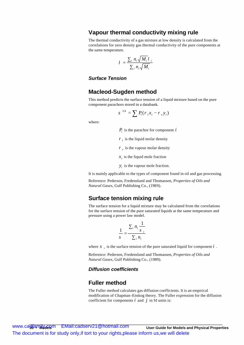
Macleod-Sugden method This method predicts the surface tension of a liquid mixture based on the pure component parachors stored in a databank.
σ ρ ρ1 4/ ( )= −∑ P x yi l i v i
where:
Pi is the parachor for component i
ρ l is the liquid molar density
ρ v is the vapour molar density
x i is the liquid mole fraction
yi is the vapour mole fraction.
It is mainly applicable to the types of component found in oil and gas processing.
Reference: Pedersen, Fredenslund and Thomassen, Properties of Oils and Natural Gases, Gulf Publishing Co., (1989).
Surface tension mixing rule The surface tension for a liquid mixture may be calculated from the correlations for the surface tension of the pure saturated liquids at the same temperature and pressure using a power law model.
11
σσ
=∑
∑
i ii
i i
n
n
where σ i is the surface tension of the pure saturated liquid for component i .
Reference: Pedersen, Fredenslund and Thomassen, Properties of Oils and Natural Gases, Gulf Publishing Co., (1989).
Diffusion coefficients
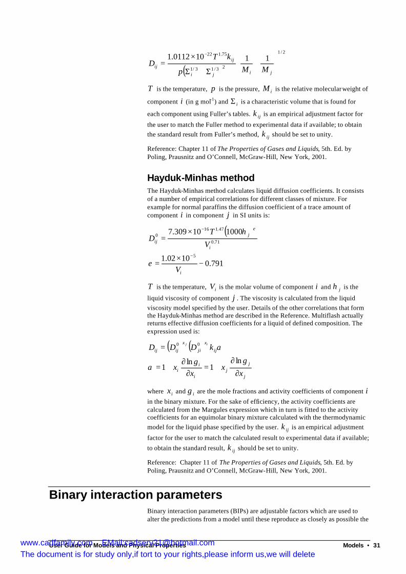
Fuller method The Fuller method calculates gas diffusion coefficients. It is an empirical modification of Chapman-Enskog theory. The Fuller expression for the diffusion coefficient for components i and j in SI units is:
www.cadfamily.com EMail:[email protected] document is for study only,if tort to your rights,please inform us,we will delete
User Guide for Models and Physical Properties Models • 31
( )
2/1
23/13/1
75.12211100112.1
+
Σ+Σ
×=
−
jiji
ijij MMp
kTD
T is the temperature, p is the pressure, iM is the relative molecular weight of
component i (in g mol-1) and iΣ is a characteristic volume that is found for
each component using Fuller’s tables. ijk is an empirical adjustment factor for
the user to match the Fuller method to experimental data if available; to obtain the standard result from Fuller’s method, ijk should be set to unity.
Reference: Chapter 11 of The Properties of Gases and Liquids, 5th. Ed. by Poling, Prausnitz and O’Connell, McGraw-Hill, New York, 2001.
Hayduk-Minhas method The Hayduk-Minhas method calculates liquid diffusion coefficients. It consists of a number of empirical correlations for different classes of mixture. For example for normal paraffins the diffusion coefficient of a trace amount of component i in component j in SI units is:
( )
791.01002.1
100010309.7
5
71.0
47.1160
−×
=
×=
−
−
i
i
jij
V
V
TD
ε
η ε
T is the temperature, iV is the molar volume of component i and jη is the
liquid viscosity of component j . The viscosity is calculated from the liquid viscosity model specified by the user. Details of the other correlations that form the Hayduk-Minhas method are described in the Reference. Multiflash actually returns effective diffusion coefficients for a liquid of defined composition. The expression used is:
( ) ( )
j
jj
i
ii
ij
x
ji
x
ijij
xx
xx
kDDD ij
∂
∂+=
∂∂
+=
=
γγα
α
ln1
ln1
00
where ix and iγ are the mole fractions and activity coefficients of component i
in the binary mixture. For the sake of efficiency, the activity coefficients are calculated from the Margules expression which in turn is fitted to the activity coefficients for an equimolar binary mixture calculated with the thermodynamic model for the liquid phase specified by the user. ijk is an empirical adjustment
factor for the user to match the calculated result to experimental data if available;
to obtain the standard result, ijk should be set to unity.
Reference: Chapter 11 of The Properties of Gases and Liquids, 5th. Ed. by Poling, Prausnitz and O’Connell, McGraw-Hill, New York, 2001.
Binary interaction parameters Binary interaction parameters (BIPs) are adjustable factors which are used to alter the predictions from a model until these reproduce as closely as possible the
www.cadfamily.com EMail:[email protected] document is for study only,if tort to your rights,please inform us,we will delete
32 • Models User Guide for Models and Physical Properties
experimental data. BIPs are usually generated by fitting experimental VLE or LLE data to the model in question, with the exception of UNIFAC, LCVM and PSRK BIPs which are predicted by group contribution. BIPs apply between pairs of components. However, the fitting procedure may be based on both binary and multi-component phase equilibria information, the former being the most common.
Number of BIPs related to any model Different models require differing numbers of BIPs and these may or may not have physical significance. The cubic equations of state (RK, RKS, PR) require only a single BIP. The closer the binary system is to ideality the smaller the size of the BIP, which will be zero for ideal systems. It is unlikely that the value of the BIP will be greater than 1, although it is possible for it to be negative. For LKP the default value of the interaction parameter is 1.
When non-standard mixing rules are used, e.g . when using RKSA(Infochem), then the number of BIPs increases. For the Gibbs excess energy type mixing rules (MHV2-type and Huron-Vidal-type) the number of BIPs will be determined by the activity coefficient model used to describe the liquid phase. For the Infochem mixing rule 3 BIPs are needed.
PC-SAFT requires two symmetric BIPs, in addition to the pure component model parameters. The default value for both is zero.
CPA uses the same interaction parameters as RKSA with the addition of three association parameters to describe cross association and self association where this occurs.
The Wilson A and UNIQUAC models require two BIPs; Wilson E needs the same number of BIPs, but these are not interchangeable with Wilson A. NRTL needs two binary energy interaction parameters and a non-randomness factor, α . With the exception of α , these BIPs may take a wide range of numerical values and more that one set may adequately represent the same experimental data. The BIPs for the activity models are asymmetric and it is important to define the binary pair of components i and j in the correct order to agree with the fitted or reported BIPs.
The NRTL α parameter defaults to 0.3 for VLE calculations and 0.2 for LLE calculations. Values derived from fitting to experimental data will vary but are unlikely to be much greater than 0.6.
The Regular Solution and Flory Huggins models both use a bipset; that is symmetrical, dimensionless and the default value is zero.
Units for BIPs The BIPs for equation of state methods are dimensionless, with the exception of two of the CPA association parameters. For some of the activity coefficient models they are dimensioned with the exception of Wilson A, Regular Solution and Flory Huggins. The dimensions used in Multiflash are J/mole. If BIPs from external sources are used in Multiflash it is important that either the BIP units are changed to match the input values or the numeric values of the BIPs are changed to J/mole.
The choice of units appears once the Units button is selected in the BIP display. J/mol is the Multiflash standard for the dimensioned activity model BIPs. Cal/mol and K are the values used in the Dechema Data Series for activity VLE and LLE BIPs. The “Aspen” format allows you to transfer the BIP values for the NRTL equation produced from Aspen Plus without further change.
www.cadfamily.com EMail:[email protected] document is for study only,if tort to your rights,please inform us,we will delete
User Guide for Models and Physical Properties Models • 33
Temperature dependence of BIPs In most of the open literature sources the reported binary interaction parameters will be temperature independent, i.e. constants. However, Multiflash allows for any BIP to be temperature dependent with either a linear or a quadratic dependence, although we do not recommend this for the NRTL α parameter.
BIPs available in Multiflash Our main BIP bank is applicable to oil and gas processing operations and called appropriately, OILANDGAS. This contains BIPs for the cubic equation of state models PR, PRA. RKS, RKSA and RKSA (Infochem) for hydrocarbons, water, methanol, glycols, H2S, CO2 and N2, and for the CPA model. The correlations have been extended to include BIPs for the LKP model for hydrocarbon and light gas mixtures. Multiflash also provides methods for estimating BIPs for the PR, RKS and CPA equations for mixtures that include petroleum fractions.
The INFOBIPS BIP bank includes BIPs for the WilsonE and the VLE variants of NRTL and UNIQUAC, based on the data reported in the Dechema Chemistry Data Series. Some BIPs are also available for equations of state such as BWRS, LKP and the cubics for systems not covered by the normal correlations, e.g. binaries including ammonia. Some of the latter have been updated in Multiflash 3.4. More systems will be added in future. A BIP bank, INFOLLBIPS, stores BIPs for use with the LLE variants of NRTL and UNIQUAC.
For the UNIFAC model , BIPs are predicted from group contributions. The data records for pure components in the INFODATA databank contain information on UNIFAC groups, where applicable, enabling the BIPs to be generated. Groups for use with the PSRK and Dortmund Modified UNIFAC models are also stored as part of the pure component UNIFAC record. Where the groups vary, Multiflash applies the correct group structure to match the chosen model. We have created an Infochem version of DIPPR that includes the same group information. You will see a warning message if the group contributions are missing for any chosen component.
It is possible to have two BIP banks in force for any problem. All the .mfc model descriptions for the equations of state define both INFOBIPS and OILANDGAS. When the model is defined Multiflash will first search INFOBIPS for any specific binary BIPS, then define BIPs from the correlations in OILANDGAS and if any are still missing they will be set to default values. The VLE variants of the activity methods only access INFOBIPS, but the LLE variants access INFOLLBIPS, followed by INFOBIPS.
Between releases of Multiflash we may amend, or add to, the BIPs stored. For the OILANDGAS databank we will supply a copy of the previous banks in order to maintain backward compatibility. The current version will still be known as OILANDGAS4, and also the default, OILANDGAS. Previous versions such as OILANDGAS3 can be recalled if you wish. For INFOBIPS we intend only to issue the latest version, if users wish to maintain access to earlier versions they should retain a copy of the relevant file.
Model data requirements Each model requires a certain amount of pure component data. These are listed in the following table.
Model Minimum input
Thermodynamic RKS critical temperature (TCRIT), critical pressure
(PCRIT), acentric factor (ACENTRICFACTOR),
www.cadfamily.com EMail:[email protected] document is for study only,if tort to your rights,please inform us,we will delete
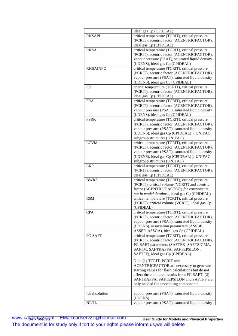
34 • Models User Guide for Models and Physical Properties
ideal gas Cp (CPIDEAL) RKSAPI critical temperature (TCRIT), critical pressure
(PCRIT), acentric factor (ACENTRICFACTOR), ideal gas Cp (CPIDEAL)
RKSA critical temperature (TCRIT), critical pressure (PCRIT), acentric factor (ACENTRICFACTOR), vapour pressure (PSAT), saturated liquid density (LDENS), ideal gas Cp (CPIDEAL)
RKSAINFO critical temperature (TCRIT), critical pressure (PCRIT), acentric factor (ACENTRICFACTOR), vapour pressure (PSAT), saturated liquid density (LDENS), ideal gas Cp (CPIDEAL)
PR critical temp erature (TCRIT), critical pressure (PCRIT), acentric factor (ACENTRICFACTOR), ideal gas Cp (CPIDEAL)
PRA critical temperature (TCRIT), critical pressure (PCRIT), acentric factor (ACENTRICFACTOR), vapour pressure (PSAT), saturated liquid density (LDENS), ideal gas Cp (CPIDEAL)
PSRK critical temperature (TCRIT), critical pressure (PCRIT), acentric factor (ACENTRICFACTOR), vapour pressure (PSAT), saturated liquid density (LDENS), ideal gas Cp (CPIDEAL) ), UNIFAC subgroup structures (UNIFAC)
LCVM critical temperature (TCRIT), critical pressure (PCRIT), acentric factor (ACENTRICFACTOR), vapour pressure (PSAT), saturated liquid density (LDENS), ideal gas Cp (CPIDEAL) ), UNIFAC subgroup structures (UNIFAC)
LKP critical temperature (TCRIT), critical pressure (PCRIT), acentric factor (ACENTRICFACTOR), ideal gas Cp (CPIDEAL)
BWRS critical temperature (TCRIT), critical pressure (PCRIT), critical volume (VCRIT) and acentric factor (ACENTRICFACTOR) for components not in model database, ideal gas Cp (CPIDEAL)
CSM critical temperature (TCRIT), critical pressure (PCRIT), critical volume (VCRIT), ideal gas Cp (CPIDEAL)
CPA critical temperature (TCRIT), critical pressure (PCRIT), acentric factor (ACENTRICFACTOR), vapour pressure (PSAT), saturated liquid density (LDENS), association parameters (ASSBE, ASSEP, ASSGA), ideal gas Cp (CPIDEAL)
PC-SAFT critical temperature (TCRIT), critical pressure (PCRIT), acentric factor (ACENTRICFACTOR), PC-SAFT parameters (SAFTEK, SAFTSIGMA, SAFTM, SAFTKAPPA, SAFTEPSILON, SAFTFF), ideal gas Cp (CPIDEAL).
Note (1) TCRIT, PCRIT and ACENTRICFACTOR are necessary to generate starting values for flash calculations but do not affect the computed results from PC-SAFT. (2) SAFTKAPPA, SAFTEPSILON and SAFTFF are only needed for associating components.
Ideal solution vapour pressure (PSAT), saturated liquid density
(LDENS) NRTL vapour pressure (PSAT), saturated liquid density
www.cadfamily.com EMail:[email protected] document is for study only,if tort to your rights,please inform us,we will delete
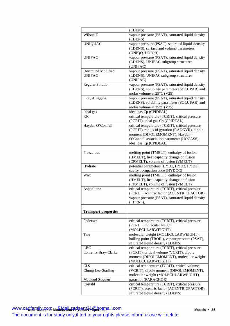
User Guide for Models and Physical Properties Models • 35
(LDENS) Wilson E vapour pressure (PSAT), saturated liquid density
(LDENS) UNIQUAC vapour pressure (PSAT), saturated liquid density
(LDENS), surface and volume parameters (UNIQQ, UNIQR)
UNIFAC vapour pressure (PSAT), saturated liquid density (LDENS), UNIFAC subgroup structures (UNIFAC)
Dortmund Modified UNIFAC
vapour pressure (PSAT), saturated liquid density (LDENS), UNIFAC subgroup structures (UNIFAC)
Regular Solution vapour pressure (PSAT), saturated liquid density (LDENS), solubility parameter (SOLUPAR) and molar volume at 25°C (V25).
Flory-Huggins vapour pressure (PSAT), saturated liquid density (LDENS), solubility para meter (SOLUPAR) and molar volume at 25°C (V25).
Ideal gas ideal gas Cp (CPIDEAL) RK critical temperature (TCRIT), critical pressure
(PCRIT), ideal gas Cp (CPIDEAL) Hayden O’Connell critical temperature (TCRIT), critical pressure
(PCRIT), radius of gyration (RADGYR), dipole moment (DIPOLEMOMENT), Hayden-O’Connell association parameter (HOCASS), ideal gas Cp (CPIDEAL)
Freeze-out melting point (TMELT), enthalpy of fusion
(HMELT), heat capacity change on fusion (CPMELT), volume of fusion (VMELT)
Hydrate potential parameters (HYD1, HYD2, HYD3), cavity occupation code (HYDOC)
Wax melting point (TMELT), enthalpy of fusion (HMELT), heat capacity change on fusion (CPMELT), volume of fusion (VMELT)
Asphaltene critical temperature (TCRIT), critical pressure (PCRIT), acentric factor (ACENTRICFACTOR), vapour pressure (PSAT), saturated liquid density (LDENS),
Transport properties Pedersen critical temperature (TCRIT), critical pressure
(PCRIT), molecular weight (MOLECULARWEIGHT)
Twu molecular weight (MOLECULARWEIGHT), boiling point (TBOIL), vapour pressure (PSAT), saturated liquid density (LDENS)
LBC Lohrentz-Bray-Clarke
critical temperature (TCRIT), critical pressure (PCRIT), critical volume (VCRIT), dipole moment (DIPOLEMOMENT), molecular weight (MOLECULARWEIGHT)
CLS Chung-Lee-Starling
critical temperature (TCRIT), critical volume (VCRIT), dipole moment (DIPOLEMOMENT), molecular weight (MOLECULARWEIGHT)
Macleod-Sugden parachor (PARACHOR) Costald critical temperature (TCRIT), critical pressure
(PCRIT), acentric factor (ACENTRICFACTOR), saturated liquid density (LDENS)
www.cadfamily.com EMail:[email protected] document is for study only,if tort to your rights,please inform us,we will delete
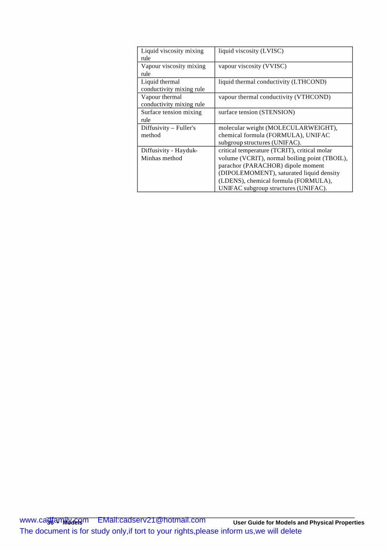
36 • Models User Guide for Models and Physical Properties
Liquid viscosity mixing rule
liquid viscosity (LVISC)
Vapour viscosity mixing rule
vapour viscosity (VVISC)
Liquid thermal conductivity mixing rule
liquid thermal conductivity (LTHCOND)
Vapour thermal conductivity mixing rule
vapour thermal conductivity (VTHCOND)
Surface tension mixing rule
surface tension (STENSION)
Diffusivity – Fuller's method
molecular weight (MOLECULARWEIGHT), chemical formula (FORMULA), UNIFAC subgroup structures (UNIFAC).
Diffusivity - Hayduk-Minhas method
critical temperature (TCRIT), critical molar volume (VCRIT), normal boiling point (TBOIL), parachor (PARACHOR) dipole moment (DIPOLEMOMENT), saturated liquid density (LDENS), chemical formula (FORMULA), UNIFAC subgroup structures (UNIFAC).
www.cadfamily.com EMail:[email protected] document is for study only,if tort to your rights,please inform us,we will delete
User Guide for Models and Physical Properties Components • 37
Components
Introduction Multiflash recognises three types of component. Normal components are pure compounds such as hydrocarbons, petrochemicals and chemicals, which may exist as gas, liquid or solid depending on conditions of temperature and pressure. A petroleum fraction is a pseudo component, usually a complex mixture of hydrocarbons, whose aggregate properties are characterised by standard tests, the results of which may be found in PVT laboratory reports. Finally, a condensed component is a pure solid phase; in Multiflash, these are used in chemical equilibrium calculations only.
The physical properties for each type of component are stored or defined differently.
Normal components The physical properties of normal components are usually stored in databanks. Multiflash offers two, INFODATA and DIPPRTM. INFODATA is the Infochem fluids databank, which contains data on about 200 compounds and is always supplied as part of Multiflash. DIPPR, produced under the auspices of AIChE, currently has data for over 1700 compounds, but is extended annually. .
Properties of normal components Both INFODATA and DIPPR store data for each variable property (e.g. vapour pressure, liquid density) of a component as a function of temperature. Properties that are not temperature dependent are stored as constant values. A list of the properties available in DIPPR and INFODATA is shown below. Some properties may be missing for individual components.
Constant properties
Molecular Weight Critical Temperature Critical Pressure Critical Volume Critical Compressibility Factor Melting Point Triple Point Temperature Triple Point Pressure Normal Boiling Point (at 1 atm) Liquid Molar Volume at 298.15K Standard Ideal Gas Enthalpy of
www.cadfamily.com EMail:[email protected] document is for study only,if tort to your rights,please inform us,we will delete
38 • Components User Guide for Models and Physical Properties
Formation at 298.15K Standard Ideal Gas Gibbs Energy of Formation at 298.15K Standard Ideal Gas Entropy at 298.15K Enthalpy of Fusion at Melting Point Entropy of Fusion at Melting Point Heat capacity change on fusion Volume change on fusion Standard Net Enthalpy of Co mbustion at 298.15K Acentric Factor Radius of Gyration Parachor Solubility Parameter at 298.15K Dipole Moment van der Waals Volume (UNIQUAC r) van der Waals Area (UNIQUAC q) Refractive Index Flash Point Lower Flammability Limit Upper Flammability Limit Autoignition Temperature
plus some model specific parameters.
Additionally there is a group of properties that allow unique identification of the name and type of the component. These are
TYPE CAS number FORMULA FAMILY code
Normal databank components will be TYPE 1.
Temperature Dependent Properties Solid Density Liquid density Vapour Pressure Enthalpy of vaporisation Solid Heat Capacity Liquid Heat Capacity Ideal Gas Heat Capacity Second Virial Coefficient Liquid Viscosity Vapour Viscosity Liquid Thermal Conductivity Vapour Thermal Conductivity Surface tension
Both databanks, in addition to the properties above, also contain the UNIFAC and PSRK group structures, where applicable. For some components, coefficients will also be stored for the second virial coefficient and relative permittivity, both used for model calculations.
INFODATA contains only a limited range of components, about 200, mainly suitable for oil and gas processing. Although every effort has been made to ensure that the data stored are correct we do not offer INFODATA as a quality assured databank.
DIPPR is developed under the auspices of the American Institute of Chemical Engineers. The databank contains a broad range of components including
www.cadfamily.com EMail:[email protected] document is for study only,if tort to your rights,please inform us,we will delete
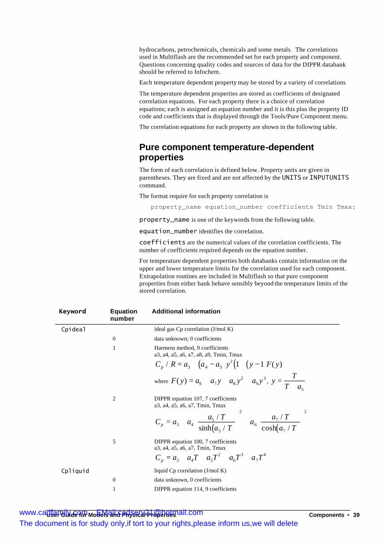
User Guide for Models and Physical Properties Components • 39
hydrocarbons, petrochemicals, chemicals and some metals. The correlations used in Multiflash are the recommended set for each property and component. Questions concerning quality codes and sources of data for the DIPPR databank should be referred to Infochem.
Each temperature dependent property may be stored by a variety of correlations
The temperature dependent properties are stored as coefficients of designated correlation equations. For each property there is a choice of correlation equations; each is assigned an equation number and it is this plus the property ID code and coefficients that is displayed through the Tools/Pure Component menu.
The correlation equations for each property are shown in the following table.
Pure component temperature-dependent properties The form of each correlation is defined below. Property units are given in parentheses. They are fixed and are not affected by the UNITS or INPUTUNITS command.
The format require for each property correlation is
property_name equation_number coefficients Tmin Tmax;
property_name is one of the keywords from the following table.
equation_number identifies the correlation.
coefficients are the numerical values of the correlation coefficients. The number of coefficients required depends on the equation number.
For temperature dependent properties both databanks contain information on the upper and lower temperature limits for the correlation used for each component. Extrapolation routines are included in Multiflash so that pure component properties from either bank behave sensibly beyond the temperature limits of the stored correlation.
Keyword Equation number
Additional information
Cpideal ideal gas Cp correlation (J/mol K)
0 data unknown; 0 coefficients
1 Harmens method, 9 coefficients a3, a4, a5, a6, a7, a8, a9, Tmin, Tmax
( ) ( )( )C R a a a y y F yp / ( )= + − + −3 4 32 1 1
where F y a a y a y a y( ) = + + +6 7 82
93 , y
TT a
=+ 5
2 DIPPR equation 107, 7 coefficients a3, a4, a5, a6, a7, Tmin, Tmax
( ) ( )C a a
a Ta T
aa T
a Tp = +
+
3 4
5
5
2
67
7
2/
sinh //
cosh /
5 DIPPR equation 100, 7 coefficients a3, a4, a5, a6, a7, Tmin, Tmax
C a a T a T a T a Tp = + + + +3 4 52
63
74
Cpliquid liquid Cp correlation (J/mol K)
0 data unknown, 0 coefficients
1 DIPPR equation 114, 9 coefficients
www.cadfamily.com EMail:[email protected] document is for study only,if tort to your rights,please inform us,we will delete
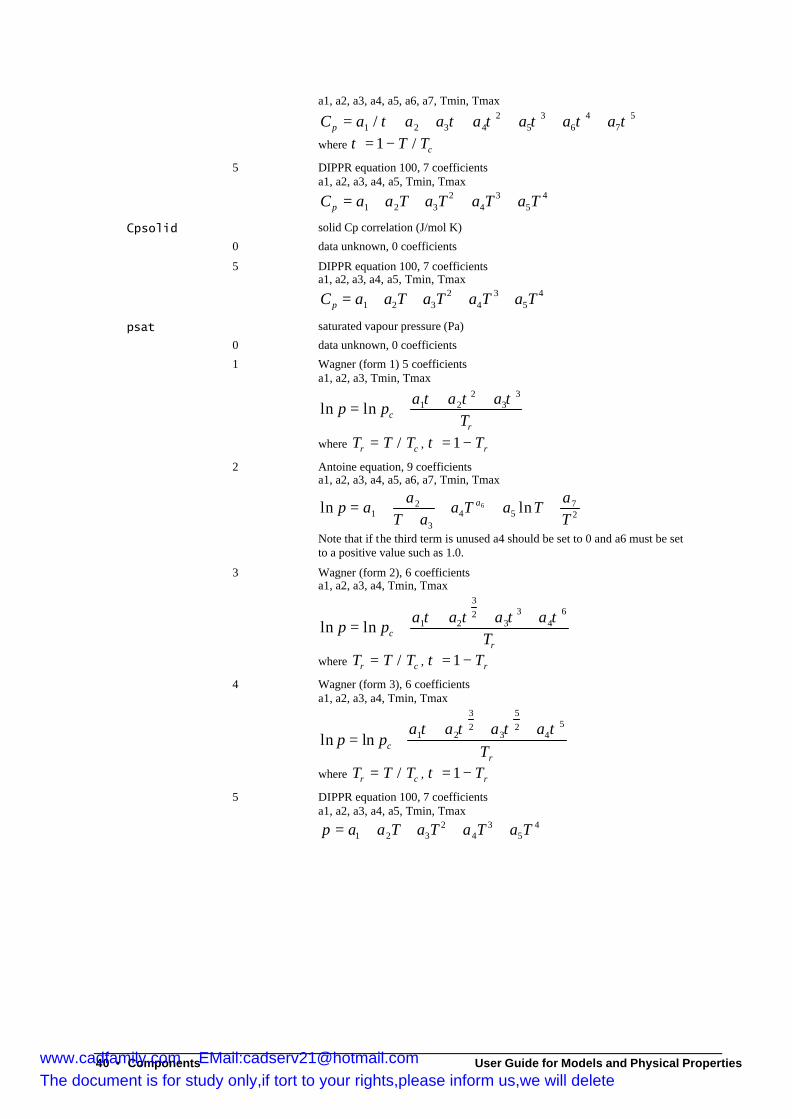
40 • Components User Guide for Models and Physical Properties
a1, a2, a3, a4, a5, a6, a7, Tmin, Tmax
C a a a a a a ap = + + + + + +1 2 3 42
53
64
75/ τ τ τ τ τ τ
where τ = −1 T Tc/
5 DIPPR equation 100, 7 coefficients a1, a2, a3, a4, a5, Tmin, Tmax
C a a T a T a T a Tp = + + + +1 2 32
43
54
Cpsolid solid Cp correlation (J/mol K)
0 data unknown, 0 coefficients
5 DIPPR equation 100, 7 coefficients a1, a2, a3, a4, a5, Tmin, Tmax
C a a T a T a T a Tp = + + + +1 2 32
43
54
psat saturated vapour pressure (Pa)
0 data unknown, 0 coefficients
1 Wagner (form 1) 5 coefficients a1, a2, a3, Tmin, Tmax
ln lnp pa a a
Tcr
= ++ +1 2
23
3τ τ τ
where T T Tr c= / , τ = −1 Tr
2 Antoine equation, 9 coefficients a1, a2, a3, a4, a5, a6, a7, Tmin, Tmax
ln lnp aa
T aa T a T
aT
a= ++
+ + +12
34 5
72
6
Note that if the third term is unused a4 should be set to 0 and a6 must be set to a positive value such as 1.0.
3 Wagner (form 2), 6 coefficients a1, a2, a3, a4, Tmin, Tmax
ln lnp pa a a a
Tcr
= ++ + +1 2
32
33
46τ τ τ τ
where T T Tr c= / , τ = −1 Tr
4 Wagner (form 3), 6 coefficients a1, a2, a3, a4, Tmin, Tmax
ln lnp pa a a a
Tcr
= ++ + +1 2
32
3
52
45τ τ τ τ
where T T Tr c= / , τ = −1 Tr
5 DIPPR equation 100, 7 coefficients a1, a2, a3, a4, a5, Tmin, Tmax
p a a T a T a T a T= + + + +1 2 32
43
54
www.cadfamily.com EMail:[email protected] document is for study only,if tort to your rights,please inform us,we will delete
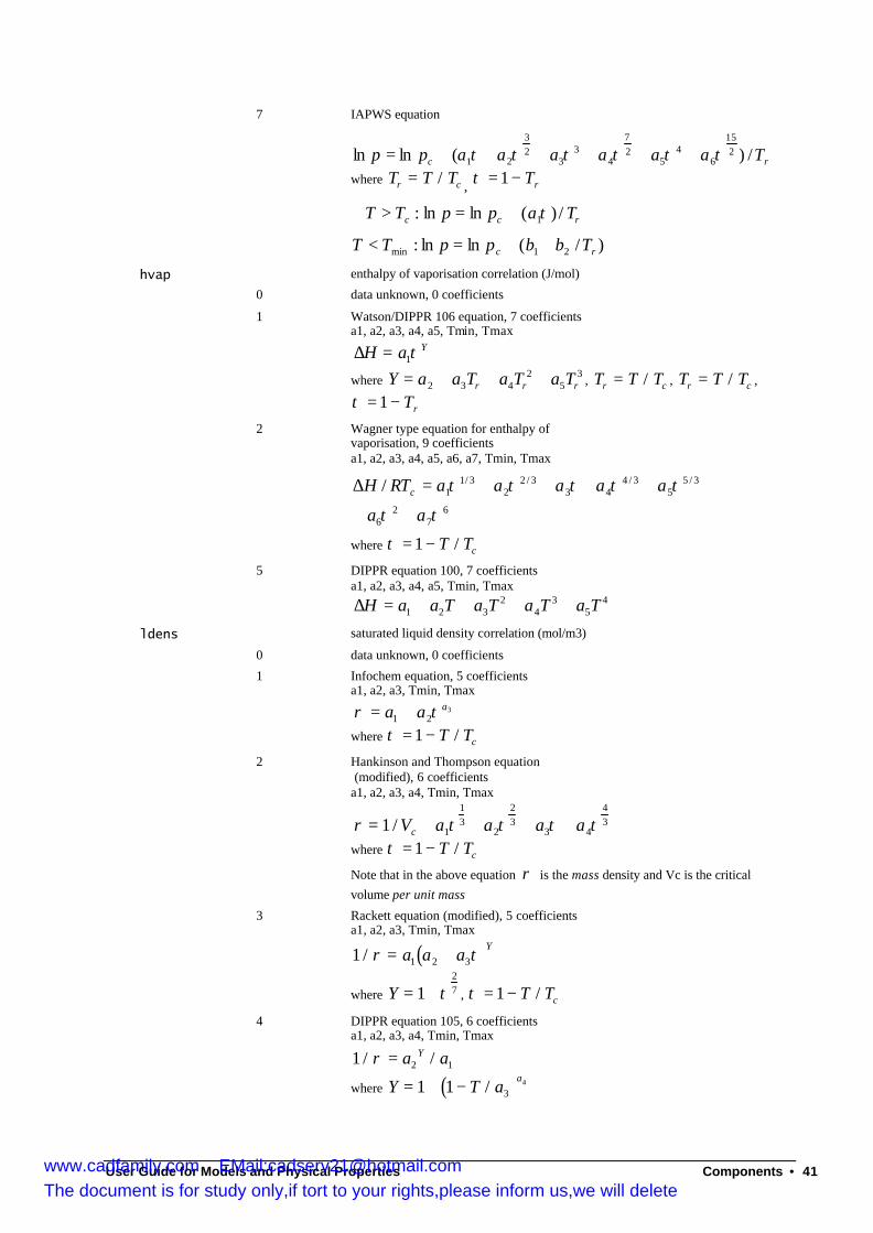
User Guide for Models and Physical Properties Components • 41
7 IAPWS equation
rc Taaaaaapp /)(lnln 215
64
527
43
323
21 ττττττ ++++++=where T T Tr c= / , τ = −1 Tr
rcc TappTT /)(lnln: 1τ+=>
)/(lnln: 21min rc TbbppTT ++=<
hvap enthalpy of vaporisation correlation (J/mol)
0 data unknown, 0 coefficients
1 Watson/DIPPR 106 equation, 7 coefficients a1, a2, a3, a4, a5, Tmin, Tmax
∆H a Y= 1τ
where Y a a T a T a Tr r r= + + +2 3 42
53 , T T Tr c= / , T T Tr c= / ,
τ = −1 Tr
2 Wagner type equation for enthalpy of vaporisation, 9 coefficients a1, a2, a3, a4, a5, a6, a7, Tmin, Tmax
67
26
3/55
3/443
3/22
3/11/
ττ
τττττ
aa
aaaaaRTH c
++
++++=∆
where τ = −1 T Tc/
5 DIPPR equation 100, 7 coefficients a1, a2, a3, a4, a5, Tmin, Tmax
∆H a a T a T a T a T= + + + +1 2 32
43
54
ldens saturated liquid density correlation (mol/m3)
0 data unknown, 0 coefficients
1 Infochem equation, 5 coefficients a1, a2, a3, Tmin, Tmax
321
aaa τρ +=
where τ = −1 T Tc/
2 Hankinson and Thompson equation (modified), 6 coefficients a1, a2, a3, a4, Tmin, Tmax
ρ τ τ τ τ= + + + +1 1
13
2
23
3 4
43/ V a a a ac
where τ = −1 T Tc/
Note that in the above equation ρ is the mass density and Vc is the critical volume per unit mass
3 Rackett equation (modified), 5 coefficients a1, a2, a3, Tmin, Tmax
( )1 1 2 3/ ρ τ= +a a aY
where Y = +127τ , τ = −1 T Tc/
4 DIPPR equation 105, 6 coefficients a1, a2, a3, a4, Tmin, Tmax
1 2 1/ /ρ = a aY
where ( )Y T aa
= + −1 1 34/
www.cadfamily.com EMail:[email protected] document is for study only,if tort to your rights,please inform us,we will delete
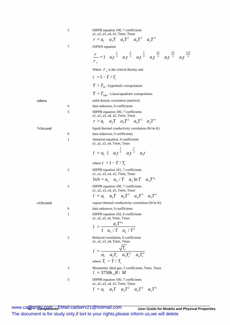
42 • Components User Guide for Models and Physical Properties
5 DIPPR equation 100, 7 coefficients a1, a2, a3, a4, a5, Tmin, Tmax
ρ = + + + +a a T a T a T a T1 2 32
43
54
7 IAPWS equation
3110
6343
53
16
435
332
231
11 ττττττρρ
aaaaaac
++++++=
Where cρ is the critical density and
τ = −1 T Tc/
HTT > : hyperbolic extrapolation
minTT < : Linear/quadratic extrapolation
sdens solid density correlation (mol/m3)
0 data unknown, 0 coefficients
5 DIPPR equation 100, 7 coefficients a1, a2, a3, a4, a5, Tmin, Tmax
ρ = + + + +a a T a T a T a T1 2 32
43
54
lthcond liquid thermal conductivity correlation (W/m K)
0 data unknown, 0 coefficients
1 Jamieson equation, 6 coefficients a1, a2, a3, a4, Tmin, Tmax
λ τ τ τ= + + +
a a a a1 2
13
3
23
41
where τ = −1 T Tc/
2 DIPPR equation 101, 7 coefficients a1, a2, a3, a4, a5, Tmin, Tmax
ln / lnη = + + +a a T a T a T a1 2 3 4
5
5 DIPPR equation 100, 7 coefficients a1, a2, a3, a4, a5, Tmin, Tmax
λ = + + + +a a T a T a T a T1 2 32
43
54
vthcond vapour thermal conductivity correlation (W/m K)
0 data unknown, 0 coefficients
1 DIPPR equation 102, 6 coefficients a1, a2, a3, a4, Tmin, Tmax
λ =+ +
a Ta T a T
a1
3 42
2
1 / /
2 Reduced correlation, 6 coefficients a1, a2, a3, a4, Tmin, Tmax
λ =+ + +
Ta a T a T a T
r
r r r1 2 32
43
where T T Tr c= /
3 Monatomic ideal gas, 2 coefficients, Tmin, Tmax λ η= 3750 0 R M/
5 DIPPR equation 100, 7 coefficients a1, a2, a3, a4, a5, Tmin, Tmax
λ = + + + +a a T a T a T a T1 2 32
43
54
www.cadfamily.com EMail:[email protected] document is for study only,if tort to your rights,please inform us,we will delete
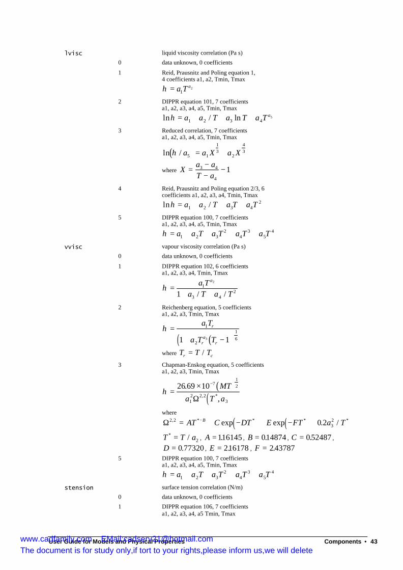
User Guide for Models and Physical Properties Components • 43
lvisc liquid viscosity correlation (Pa s)
0 data unknown, 0 coefficients
1 Reid, Prausnitz and Poling equation 1, 4 coefficients a1, a2, Tmin, Tmax
η = a T a1
2
2 DIPPR equation 101, 7 coefficients a1, a2, a3, a4, a5, Tmin, Tmax
ln / lnη = + + +a a T a T a T a1 2 3 4
5
3 Reduced correlation, 7 coefficients a1, a2, a3, a4, a5, Tmin, Tmax
( )ln /η a a X a X5 1
13
2
43= +
where Xa aT a
=−−
−3 4
4
1
4 Reid, Prausnitz and Poling equation 2/3, 6 coefficients a1, a2, a3, a4, Tmin, Tmax
ln /η = + + +a a T a T a T1 2 3 42
5 DIPPR equation 100, 7 coefficients a1, a2, a3, a4, a5, Tmin, Tmax
η = + + + +a a T a T a T a T1 2 32
43
54
vvisc vapour viscosity correlation (Pa s)
0 data unknown, 0 coefficients
1 DIPPR equation 102, 6 coefficients a1, a2, a3, a4, Tmin, Tmax
η =+ +
a Ta T a T
a1
3 42
2
1 / /
2 Reichenberg equation, 5 coefficients a1, a2, a3, Tmin, Tmax
( )( )η =
+ −
a T
a T T
r
ra
r
1
2
161 13
where T T Tr c= /
3 Chapman-Enskog equation, 5 coefficients a1, a2, a3, Tmin, Tmax
( )( )η =
× −26 69 10 712
12 2 2
3
.
,, *
MT
a T aΩ
where
( ) ( )Ω2 2320 2, * * * *exp exp . /= + − + − +−AT C DT E FT a TB
T T a* /= 2 , A = 116145. , B = 014874. , C = 0 52487. ,
D = 0 77320. , E = 216178. , F = 2 43787.
5 DIPPR equation 100, 7 coefficients a1, a2, a3, a4, a5, Tmin, Tmax
η = + + + +a a T a T a T a T1 2 32
43
54
stension surface tension correlation (N/m)
0 data unknown, 0 coefficients
1 DIPPR equation 106, 7 coefficients a1, a2, a3, a4, a5 Tmin, Tmax
www.cadfamily.com EMail:[email protected] document is for study only,if tort to your rights,please inform us,we will delete
44 • Components User Guide for Models and Physical Properties
( )σ = −a TrY
1 1
where Y a a T a T a Tr r r= + + +2 3 42
53 , T T Tr c= /
2 Extended Sprow and Prausnitz equation, 5 coefficients a1, a2, a3, Tmin, Tmax
( )σ τ τ= +a aa1 3
2 1
where τ = −1 T Tc/
5 DIPPR equation 100, 7 coefficients a1, a2, a3, a4, a5, Tmin, Tmax
σ = + + + +a a T a T a T a T1 2 32
43
54
virialcoeff second virial coefficient correlation (m3/mol)
0 data unknown, 0 coefficients
1 DIPPR equation 104, 7 coefficients a1, a2, a3, a4, a5 Tmin, Tmax
B a a a a a= + + + +1 2 33
48
59τ τ τ τ
where τ = T Tc /
5 DIPPR equation 100, 7 coefficients a1, a2, a3, a4, a5, Tmin, Tmax
B a a T a T a T a T= + + + +1 2 32
43
54
Petroleum fractions To define a single petroleum fraction the program requires certain characteristic properties and Multiflash will then estimate the other properties needed to support the range of calculations available in the program.
The list of possible properties to support characterisation of the fraction are:
Carbon number
Molecular weight (g/mol)
Specific gravity at 60oF relative to water at 60oF
Normal boiling point
Critical temperature
Critical pressure
Pitzer’s acentric factor
However, not all of these are necessary. The minimum input sets are molecular weight, molecular weight and specific gravity; molecular weight and boiling point; boiling point and specific gravity; critical temperature, critical pressure and acentric factor. Alternatively, the boiling point can be used instead of the acentric factor.
The properties that are estimated, if they have not been provided, are:
Carbon number
Molecular weight
Normal boiling point
Critical temperature
Critical pressure
Critical volume
www.cadfamily.com EMail:[email protected] document is for study only,if tort to your rights,please inform us,we will delete
User Guide for Models and Physical Properties Components • 45
Acentric factor
Parachor
Dipole moment
Enthalpy of formation
Standard entropy
Perfect gas Cp
Saturated liquid density
Saturated vapour pressure
Enthalpy of evaporation
Liquid viscosity
Petroleum fractions will normally be designated as TYPE 12.
Property Calculation The order in which properties are calculated depends on the amount of input data provided. In general the following references are used as a basis for the calculations:
Molecular weight Riazi, M.R. and Al-Sahhaf, T.A., Fluid Phase Equilibria 117 217-224 (1996)
Boiling point Edmister, W.C. Pet. Refiner 37 154 (1958) Brule, M.R. and Whitson, C.H., SPE Monograph 20 (2000) Riazi, M.R. and Al-Sahhaf, T.A., Ind. Eng. Chem. Research, 34 4145 (1995)
Specific gravity Riazi, M.R. and Al-Sahhaf, T.A., Ind. Eng. Chem. Research, 34 4145 (1995)
Tc, Pc, ω Kesler, M.G. and Lee, B.I., Hydrocarbon Processing 55(3) 153 (1976)
Brule, M.R. and Whitson, C.H., SPE Monograph 20 (2000)
Riazi, M.R. and Al-Sahhaf, T.A., Ind. Eng. Chem. Research, 34 4145 (1995
Vc Riazi, M.R., Daubert, T.E., Hydrocarbon Processing, 59, 115 (1980)
Lira -Galeana, C., Firoozabadi, A. and Prausnitz, J.M., AIChE J., 42(1) 239 (1996)Riazi, M.R. and Al-Sahhaf, T.A., Ind. Eng. Chem. Research, 34 4145 (1995)
Enthalpy of Formation and Standard Entropy Reid, R.C., Prausnitz, J.M. and Poling, B.E.;
"The Properties of Gases and Liquids", Gulf, Houston (1987)
Ideal Cp Kesler, M.G. and Lee, B.I., Hydrocarbon Processing 55(3) 153 (1976) and
Harmens, A., "Chemical Thermodynamics Data on Fluids and Fluid Mixtures", IPC Science and Technology Press (1979)
Melting Point Won, K.W., Fluid Phase Equilbria , 30 265 (1986) Lira -Galeana, C., Firoozabadi, A. and Prausnitz, J.M.,
AIChE J., 42(1) 239 (1996)
www.cadfamily.com EMail:[email protected] document is for study only,if tort to your rights,please inform us,we will delete
46 • Components User Guide for Models and Physical Properties
Fusion properties Morgan, D.L. and Kobayashi, R., Fluid Phase Equilibria, 63 317 (1991)
Won, K.W., Fluid Phase Equilbria , 30 265 (1986) Brown, T.S., Niesen, V.G. and Erikson, D.D., SPE
8505 (1994) Lira -Galeana, C., Firoozabadi, A. and Prausnitz, J.M.,
AIChE J., 42(1) 239 (1996)
Solubility Parameter Pedersen, K.S., et al, Energy and Fuels. 5 924 (1991)
Surface Tension Quale, O.R., Chem. Rev ., 53 439 (1958)
Liquid Viscosity Orbey, H. and Sandler, S.I., Canadian J. Che. Eng., 74 437 (1993)
Condensed components The INFOCOND databank includes about 140 solid compounds. The data are limited to molecular weight, normal melting point, normal boiling point, the enthalpy of formation in the condensed state at 298.15K, the standard entropy in the condensed state at 298.15K and the heat capacity in the condensed state as a function of temperature. It is intended for use with Infochem's chemical and phase equilibrium module, Chemreact.
www.cadfamily.com EMail:[email protected] document is for study only,if tort to your rights,please inform us,we will delete

User Guide for Models and Physical Properties Components • 47
www.cadfamily.com EMail:[email protected] document is for study only,if tort to your rights,please inform us,we will delete

www.cadfamily.com EMail:[email protected] document is for study only,if tort to your rights,please inform us,we will delete
User Guide for Models and Physical Properties Index • 49
Index
C
Cubic plus association (CPA) model 9
D
Diffusion coefficients 30
M
Models 32 Binary interaction parameters (BIPs) 32
N
Nucleation model 24
S
Surface tension 30
T
Thermal conductivity 29
V
Viscosity 27
W
Wilson A equation 17
www.cadfamily.com EMail:[email protected] document is for study only,if tort to your rights,please inform us,we will delete